On the Expected Performance of Market Timing Strategies · On the Expected Performance of Market...

42 ON THE EXPECTED PERFORMANCE OF MARKET TIMING STRATEGIES SUMMER 2014

On the Expected Performance of Market Timing StrategiesWINFRIED G. HALLERBACH

WINFRIED G. HALLERBACH

is a senior researcher atQuantitative Strategies, Robeco Investment Man-agement, in Rotterdam, The [email protected]

Grinold’s [1989] Fundamental Law of Active Management (FLAM) is a key analysis tool for active strate-gies. FLAM relates the maximum

attainable information ratio (IR) of an active strategy to skill and breadth: IR IC Brearr dth≈ . The information coefficient (IC) is the cor-relation between forecasted and subsequent realized returns and represents skill. Breadth is the total number of distinct bets taken over a year and over separate strategies. Grinold repeatedly stresses that his FLAM is not an operational tool but is designed to provide fundamental insight into active management: “It is important to play often (high breadth) and to play well (high IC)” (Grinold and Kahn [2000, p. 157]).

Numerous papers have discussed and extended the original FLAM. For example, Qian and Hua [2004] and Ye [2008] study the effect of variation in the IC. Buckle [2004] covers correlated forecasts, Zhou [2008a] focuses on estimation risk, and Lam and Li [2004] and Zhou [2008b] analyze unconditional optimality in the context of the FLAM.

In this article, we apply the FLAM to market timing. A timing strategy entails switching between net long and short posi-tions in markets, sectors, or even individual assets, in the hope of reaping outperformance. Skill depends on the success ratio: the prob-ability of correctly forecasting the market’s

direction. Market timing is hard. Neuhierl and Schlusche [2010] investigate a compre-hensive set of simple and complex timing rules and conclude that, although successful timing rules exist, their outperformance does not remain signif icant after correcting for potential biases from data snooping. Various empirical studies show that a sizeable success ratio of at least 66% (Bauer and Dahlquist [2001]) or at least 70% (Sharpe [1975]) would be required to beat the buy-and-hold bench-mark. In contrast, Sy [1990] argues that a success ratio of 60% suffices to outperform the benchmark. It is therefore interesting to know what IR could be expected from an implemented timing strategy and what suc-cess ratio would be required to match the timing IR with the Sharpe ratio of the buy-and-hold position.

We start with proportional, or linear, strategies (where the size of the timing posi-tion depends on the magnitude of the fore-casted return) and show that the conventional FLAM applies unabated. The main focus of the article, however, is on the more common switching strategies, where directional fore-casts result in unit long or short positions. We show that we have to make non-trivial adjustments to the expression for the IR when applying directional forecasts. In addition, we show that it is important to distinguish between time-series breadth (timing fre-quency, or how many timing bets you take per

JPM-HALLERBACH.indd 42JPM-HALLERBACH.indd 42 7/19/14 8:27:25 AM7/19/14 8:27:25 AM

IT IS IL

LEGAL TO REPRODUCE THIS A

RTICLE IN

ANY FORMAT

Copyright © 2014

THE JOURNAL OF PORTFOLIO MANAGEMENT 43SUMMER 2014

year) and cross-section breadth (the number of positions that are subject to timing) because they contribute dif-ferently to the expected IR. We show that we can maxi-mize the contribution of cross-section breadth to the IR by implementing volatility-weighted bet sizes.

We next present some extensions to the basic switching framework by allowing for neutral positions, time-varying volatility, and fat tails. We show that the negative effect of time-varying volatility on the timing IR can be reduced by volatility weighting over time (consistent with Hallerbach [2012]); this increases the contribution of time-series breadth to the timing IR. We show to what extent the presence of fat tails reduces the timing IR. Overall, we lift Grinold’s [1989] results to an operational level, where the derived IRs hold as accurate approximations. We confirm the accuracy of our findings by verifying results reported in the litera-ture and by simulating timing strategies for equities and fixed income.

Our results can be used as a reality check and benchmark against which the actual IR—learned by back-testing a timing strategy—can be compared. Given the timing frequency, the performance of a directional timing strategy depends on the success ratio (which defines the IC), as well as on the returns that are (on average) realized when the forecasts are correct and when the forecasts are wrong. Our expected IR is a benchmark IR because we do account for the effect of the success ratio, but at the same time we also assume that average returns from correct and incorrect forecasts are of equal magnitude. When the back-test IR is mark-edly higher than the expected IR, this calls for scrutiny and a detailed analysis of the sources of this outperfor-mance. It could be the case that the switching strategy was not only successful in forecasting the correct sign of the market return, according to the success ratio, but was also successful in forecasting the relative magnitude of future returns. Hence, the strategy did benefit from some large positive or negative returns by appropriate positioning, or the strategy was able to avoid some large negative returns when the forecasts turned out wrong. This additional success factor lifts the actual timing IR beyond the expected IR. The mechanisms behind this success factor should be well understood and backed by an economic story, in order to strengthen the belief that the success factor will prevail in the future. After all, a discrepancy between the actual and expected IR could likewise point at the inf luence of some extreme returns,

combined with luck (see, for example, Estrada [2009]) or data snooping, or at the effect of pure sampling error. In the latter cases, one may expect that in the future, the IR will drop to its expected level, when the success ratio is maintained, or even lower, when predictive accuracy is impaired. Finally, the expected IR can be compared with the Sharpe ratio of the buy-and-hold position, in order to infer what success ratio would be required to render timing an outperforming strategy. Because our results are special cases of the FLAM, we start with outlining this foundation of active management.

THE FUNDAMENTAL LAW OF ACTIVE MANAGEMENT

We define the outright position as a self-financing portfolio that is long the risky asset (the market) and short the risk-free position. Alternatively, the outright position is a fixed combination of long asset A and short asset B. We consider returns over N equally sized periods Δt per year, so N ⋅ Δt = 1. We write the excess return on the outright position as

� �r ttΔr Δσ ε (1)

where �ε is a zero-mean unit-variance disturbance. We assume that we have information on the next period’s excess return in the form of a standardized forecast signal, or z-score �z . The skill in forecasting excess returns is measured by the correlation between the signal and the subsequent excess return; this is information coefficient, IC. We denote the information we do not know as the noise term �η, where �η is independent of the signal �z, with E( )� =) 0 and variance E ICII( )� 2 2ICI) . Hence, � � �ε η+IC . This allows us to express the excess return as

�r ttΔr Δ ( )� �IC +σ ttt (IC z⋅IC + (2)

Alpha is the expected excess return conditional on the signal z� :

( , )t t IC z( )|z zt �|α Δ( ,, |z = σ Δ ⋅t (3)

The variance of alpha (or the variance of the fore-cast errors) is the variance of the excess return condi-tional on z:



( , ) var2 2t ( )2IC( )||r |t |ω Δ( ,, var (r | Δ (1rr (4)

Now consider an active strategy defined by the weight h(z), which is a function of the signal z. Fol-lowing Grinold and Kahn [2000], we assume mean– variance preferences with active risk-aversion parameter λ. The optimal strategy maximizes the conditional value added:

max ( ) ( ) ( )12

( ) ( )( )

2 2( )z h) z( h z(h z(

( )z) − λ1 ω (5)

We find the optimal weight by setting the first derivative of VA(z) with respect to h(z) equal to zero, yielding the well-known result:

*( )( )( )2h z*( = α

λω (6)

Using this weight in Equation (5), the maximum attainable conditional value added is:

*( )1

2( )2VA I) R(II

λ (7)

where the conditional IR is defined by the conditional expected active return divided by the active risk:

( )( )( )

2

2IR = αω

(8)

The FLAM, as formulated by Grinold [1989], states that the maximum ex ante value added is proportional to the ex ante unconditional IR squared, or

( )( )

2

2IR E= αω

⎛⎝⎜⎛⎛⎝⎝

⎞⎠⎟⎞⎞⎠⎠

(9)

where the expectation is taken with respect to all pos-sible values of �z. When assuming that the conditional variance is constant (as do Grinold and Kahn [2000]), the annualized unconditional ex ante IR follows by sub-stituting Equations (3) and (4) in Equation (9):

1

2 2 2

2 2IR EIC z IC

ICN

�( )21 IC

= σσ2 (11

⎛

⎝⎜⎛⎛

⎝⎝

⎞

⎠⎟⎞⎞

⎠⎠=

− (10)

where N is the timing frequency. Because in practice the IC is small, the denominator is approximately equal to unity (so we in effect ignore the risk reduction from using forecasts), and we obtain the FLAM:

IR IC N≈ ⋅IC (11)

Hence, the FLAM states that the maximum attain-able IR is the product of the IC (or how well you play) and the square root of breadth, N (or how often you play).

Given these ex ante results, we next consider the ex post IR, or the risk-adjusted perfor mance one may expect from realized returns on an implemented timing strategy. In the vein of the FLAM, we f irst consider bet sizes that are proportional to the timing signal. We show that the IR of these linear strategies can be adequately proxied by the conventional expres-sion (shown in Equation (11)) of the FLAM. We then switch to directional forecasts and corresponding unit long–short bet sizes.

PROPORTIONAL BET SIZES

When we have confidence in the strength of the signal �z , we can employ proportional bet sizes. The larger the signal, the larger the long or short position we take. As derived in Equation (6), the optimal bet size for signal �z is proportional to

*( )( )( )2h z*(

IC z

t

�( )1 2I1 C

∝ αω

= ⋅σ Δ

(12)

where the last equality follows from substituting Equa-tions (3) and (4). Using these bet sizes and Equation (2), the strategy return is

*( )1

2 2

2r h r)IC z I2 C z

ICts

t*(h ��

*(h ) = IC η−Δ Δ( )r h r)t (h ) (13)

As derived in the Appendix, the annualized uncon-ditional mean and variance of the strategy return are

EIC

ICN( )r s� =

−

2

21 (14)



and

var1

1 (1 )2

22IC

ICN( )r s� =

−(1 γ ⋅) (15)

where γ is the excess kurtosis of the signal �z (i.e., of the forecasted excess return). Hence, the unconditional IR is:

1 (1 )2IR

ICN IC N=

(1 γ⋅ ≤N (16)

Because in practice IC is small, the effect of excess kurtosis γ is very limited, and the upper bound holds tightly. We conclude that when timing bet sizes are proportional to the timing signal, then the IR according to the conventional FLAM provides a good approximation.

DIRECTIONAL FORECASTS

We next consider the case where only the sign of the signal is used to switch between equally sized long and short positions. When �z is positive, we forecast the subsequent excess return to be positive ( )tΔ

+ , and hence we take a long position. When the signal is negative, we forecast a negative excess return ( )tΔ and we take a short position. For simplicity, we assume that �r rt tΔ Δr rt r− +� and that the risk premium on the market over the period Δt is zero, implying that the probability of the market going up or down is ½. The probability that the forecast is right is the success ratio p. Because we are using direc-tional forecasts, the IC is now the correlation between the forecasted sign of the market return and the sign of the subsequent realized return. The IC is related to the success ratio p as IC = 2p – 1 (see Appendix).

Exhibit 1 outlines the returns of the timing strategy and the associated probabilities. There are four quad-rants, which cover the instances in which the market

goes up or down and the forecast is right or wrong. Given the timing positions and the market’s possible up and down moves, we can work out the timing strategy return, conditional on being right or wrong.

Over the period Δt, the unconditional timing strategy return is

(1 )r p r p(1 r IC rts

t t)p(1 r t� �s � �ICp r )p rΔ Δr pr rrt p r Δr IC rtrr (17)

Because the switching strategy uses only the sig-nal’s sign, the timing return now depends on the market return’s absolute value. In order to obtain tractable results, we assume that the excess market return follows a normal distribution. As derived in the Appendix, the annualized expected timing return is

2

E IC N( )r s� =π

σ (18)

and the annualized variance of the timing return is

var22 212

I11 C( )r s� σπ

⎡⎣⎣⎣

⎤⎦⎥⎤⎤⎦⎦ (19)

Hence, the annualized IR of the timing strategy is

�= =

− π( )�

var ( ) /π 2

22

IRE(�

r

IC

ICN I≈ C N

s

s

(20)

where π ≈2/π 0.798. Hence, we must apply a discount of about 20% on the IR according to the FLAM, in order to approximate the IR from a directional timing strategy under normality. This indicates that the skill of forecasting the size of the market’s return is 25% more valuable in terms of IR than the skill of forecasting the market’s direction (since 1/0.8 = 1.25).

E X H I B I T 1Directional Timing Strategy Positions and Returns (p is the success ratio)



CROSS-SECTION VERSUS TIME-SERIES BREADTH

In the remainder, we focus on directional fore-casts. The timing frequency per year is the time series breadth N. When we apply timing strategies to more than one market, we extend the cross-section breadth. Assume M markets with annualized excess returns rirr , expected returns E i( )rirr , and variances σi

2 . The return on the equally weighted portfolio of markets is simply the sum of the M market returns. We assume that both the returns and the signals on the M markets are uncor-related.1 The expected return on the combined timing strategies is simply the sum of the individual strategies’ expected returns E i

s( )rirrs , and the variance is the sum of

the individual timing strategies’ variances var( )�rirrs . The

expected IR of the combined timing portfolio equals

( )

var( )IR

E(

r

s is

i M

irrs

i M�

∑∑

= (21)

We assume a uniform timing frequency N. Under normality, the expected IR of the combined timing strategies then readily follows, by substituting Equations (18) and (19) in Equation (21):

=π −

⋅ ≈π

⋅/2

22

IRIC

ICN X⋅ IC NX (22)

where X is the effective cross-section breadth, defined as

2X M

ii

ii

∑∑

σ

σ≤ (23)

The inequality is implied by Jensen’s inequality. It holds as a strict equality when all outright volatili-ties are equal, σ

i = σ

j, ∀i, j ∈ M, in which case X = M.

The higher the dispersion in volatilities, the lower the effective breadth.2 We conclude that for uncorrelated markets and uncorrelated timing bets, 1) the effective cross-section breadth X has an upper bound of M, and 2) we can move toward this upper bound by reducing the cross-section range of market volatilities. We can achieve the latter by normalizing the individual mar-kets on which timing is performed, or equivalently by implementing volatility-weighted bet sizes. This equates

volatilities and maximizes the expected IR since then X = M holds.

SOME EXTENSIONS

Before we move to the empirical section, we present three generalizations of previous results on directional forecasts. The proofs of our statements and expressions are available in an online Appendix. The extensions cover neutral positions, time-varying vola-tility, and fat tails.

First, we allow for neutral positions (for example, when the timing signal does not exceed a certain threshold). In addition to the success ratio p, we define the probability q of incorrect directional forecasts (the failure ratio), so the probability of a neutral position follows as n = 1 – p – q. In that case, we have IC = p – q and the expected IR in Equation (22) becomes

(1 )

2(1 )2

2IR

IC

n I) CNX

nIC NX=

−n)≈

π −(1π (24)

This expression shows that the IR increases with the fraction n of neutral positions. The intuition is that, whereas the expected strategy return depends on the difference between the success and failure ratios (i.e., the IC, which we assume constant), the volatility of the strategy return depends on the sum of the success and failure ratios (i.e., the total fraction of positions actually taken). Hence, when the fraction of neutral positions increases, the expected timing return stays the same, but the timing volatility decreases, increasing the expected timing IR.

Second, we focus on time-varying volatility. Until now, we assumed that the volatility of the market returns is constant over time. In reality, financial market vola-tilities vary over time. To accommodate time-varying volatility, we assume a simplified set-up where over the N timing periods per year, N

L periods fall under a low

market volatility σL regime and N

H under a high vola-

tility σH regime (so N

L + N

H = N ).3 We also assume that

the success ratio is independent of the volatility regime. In that case the timing IR becomes

(1 )22 2

IRa IC

n a) ICN=

−n)π (25)



where a = (NLσ

L + N

Hσ

H)/(Nσ) and where σ is the

aggregate market volatility per annum over the full N periods. It can be shown that this IR is maximized when a reaches its maximum value of unity. This in turn implies that σ

L = σ

H = σ: the market volatility is constant

over the regimes. Hence, if we smooth the volatility of the underlying market over time by implementing volatility-weighted bet sizes, we increase the timing IR towards Equation (24). The better our conditional vola-tility forecasts, the more constant the volatility of the normalized market will be and the higher the timing IR. Indeed, volatility-weighted bet sizes are widely applied in practice, and together with Hallerbach [2012], this provides a theoretical basis.

Third, we escape from the restrictive normal dis-tribution setting. It is a universally accepted stylized fact that distributions of f inancial market returns exhibit fatter tails than the normal distribution does. Since the pioneering work of Praetz [1972], the t-distribution is recognized as a relatively simple alternative distribu-tion that accommodates fat tails and leptokurtosis. For a t-distribution with ν degrees of freedom (dgf ), excess kurtosis K equals K = 6/(ν − 4), for ν > 4. Hence, given the excess kurtosis of excess market returns, we can esti-mate the dgf from ν = 6/K + 4. In empirical work, the estimated dgf are about ν = 5 (for example, see Zumbach [2006] and the next section), corresponding to K = 6. When the returns on the outright markets follow t-distributions with the same dgf ν, the expected IR becomes

( )

1( )2

IRIC

k n(1 ICNX

k n(1IC NX=

−)n≈

ν ν

(26)

where kν is a scaling factor inversely related to the dgf.4 For ν =5, we have k

5 =1.851. This is larger than the

scaling factor under normality (k∞ = π/2 ≈ 1.571) and reduces the expected timing IR by about 8%. The reason that excess kurtosis reduces the IR is that the switching return is a function of the market return’s absolute value. When excess kurtosis increases, the expected value of this absolute return increases at a slower pace than its standard deviation, lowering the IR. This contrasts with the case of proportional bet sizes, where the timing return in Equation (13) is a function of the squared forecasted market return, and where the impact of excess kurtosis was shown to be almost negligible.

EMPIRICAL ILLUSTRATION

Polbennikov et al. [2010] simulate active strategies with a success ratio of 52.5% where the market return distribution is fat-tailed, according to a t-distribution with 5 dgf. For a single strategy they report an IR of 0.13, which conforms nicely to the value of 0.127 that follows from our Equation (26).

Shen [2003] tests directional timing strategies on the S&P 500, driven by the spread between the S&P 500 E/P ratio on the one hand and the three-month Treasury bill yield or ten-year Treasury bond yield on the other. Using monthly data over the period from January 1970 to December 2000, he finds annualized Sharpe ratios of 0.71 and 0.60 for the respective strategies. Given the reported success ratios of 61.8% and 59.1%, and assuming t(5)-distributions, we expect timing IRs of 0.61 and 0.47, respectively. The discrepancy between the actual and expected IRs indicates that the strategies are able to predict larger-than-average returns when the timing forecast is correct, to avoid larger-than-average negative returns when the forecast is wrong, or both. Further analysis should point out whether this additional suc-cess factor of the timing strategies is real, can be backed by an economic story and reasonably extended into the future, or only apparent (and due to luck, sampling error, or data snooping).

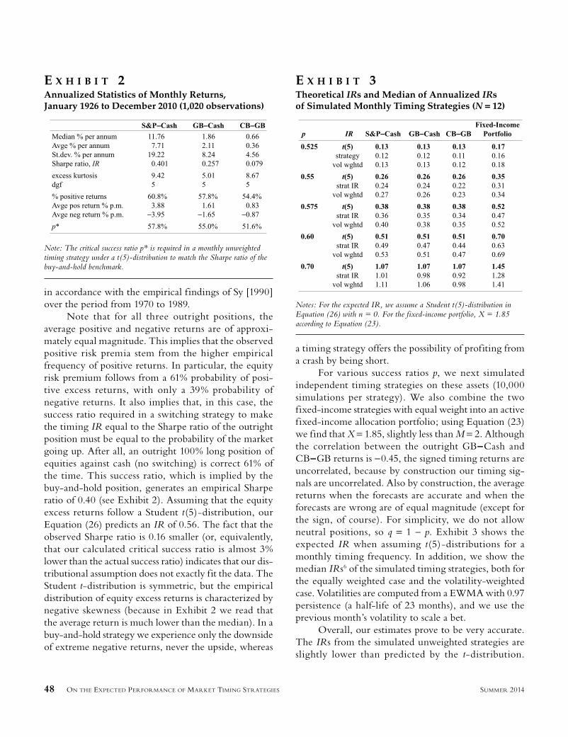
To further corroborate our theoretical f indings, we next consider monthly timing strategies on posi-tions in the S&P 500 against cash (T-bills), U.S. long-term government bonds against cash (GB−Cash), and U.S. long-term corporate bonds against U.S. long-term government bonds (CB−GB). The monthly return data span the period from January 1926 to December 2010 and are taken from Ibbotson [2010]. Exhibit 2 shows the descriptive statistics.

Over this period, the U.S. equity risk premium was just shy of 8%, translating into a Sharpe ratio of 0.40. Treasuries carried a risk (term) premium of 2%, whereas the default risk premium was only 36 basis point per annum.5 All three series exhibit excess kurtosis, consis-tent with 5 dgf when assuming t-distributions. Exhibit 2 also shows the critical success ratio p*. This is the success ratio for which the expected IR of a monthly timing strategy under a Student t(5)-distribution is equal to the Sharpe ratio of the underlying market. For the S&P 500, the critical success ratio is just shy of 60%; this is



in accordance with the empirical findings of Sy [1990] over the period from 1970 to 1989.

Note that for all three outright positions, the average positive and negative returns are of approxi-mately equal magnitude. This implies that the observed positive risk premia stem from the higher empirical frequency of positive returns. In particular, the equity risk premium follows from a 61% probability of posi-tive excess returns, with only a 39% probability of negative returns. It also implies that, in this case, the success ratio required in a switching strategy to make the timing IR equal to the Sharpe ratio of the outright position must be equal to the probability of the market going up. After all, an outright 100% long position of equities against cash (no switching) is correct 61% of the time. This success ratio, which is implied by the buy-and-hold position, generates an empirical Sharpe ratio of 0.40 (see Exhibit 2). Assuming that the equity excess returns follow a Student t(5)-distribution, our Equation (26) predicts an IR of 0.56. The fact that the observed Sharpe ratio is 0.16 smaller (or, equivalently, that our calculated critical success ratio is almost 3% lower than the actual success ratio) indicates that our dis-tributional assumption does not exactly fit the data. The Student t-distribution is symmetric, but the empirical distribution of equity excess returns is characterized by negative skewness (because in Exhibit 2 we read that the average return is much lower than the median). In a buy-and-hold strategy we experience only the downside of extreme negative returns, never the upside, whereas

a timing strategy offers the possibility of profiting from a crash by being short.

For various success ratios p, we next simulated independent timing strategies on these assets (10,000 simulations per strategy). We also combine the two fixed-income strategies with equal weight into an active fixed-income allocation portfolio; using Equation (23) we find that X = 1.85, slightly less than M = 2. Although the correlation between the outright GB−Cash and CB−GB returns is −0.45, the signed timing returns are uncorrelated, because by construction our timing sig-nals are uncorrelated. Also by construction, the average returns when the forecasts are accurate and when the forecasts are wrong are of equal magnitude (except for the sign, of course). For simplicity, we do not allow neutral positions, so q = 1 – p. Exhibit 3 shows the expected IR when assuming t(5)-distributions for a monthly timing frequency. In addition, we show the median IRs6 of the simulated timing strategies, both for the equally weighted case and the volatility-weighted case. Volatilities are computed from a EWMA with 0.97 persistence (a half-life of 23 months), and we use the previous month’s volatility to scale a bet.

Overall, our estimates prove to be very accurate. The IRs from the simulated unweighted strategies are slightly lower than predicted by the t-distribution.

E X H I B I T 3Theoretical IRs and Median of Annualized IRs of Simulated Monthly Timing Strategies (N = 12)

E X H I B I T 2Annualized Statistics of Monthly Returns, January 1926 to December 2010 (1,020 observations)

Note: The critical success ratio p* is required in a monthly unweighted timing strategy under a t(5)-distribution to match the Sharpe ratio of the buy-and-hold benchmark.

Notes: For the expected IR, we assume a Student t(5)-distribution in Equation (26) with n = 0. For the fixed-income portfolio, X = 1.85 according to Equation (23).



We would expect this because volatility is clearly not constant over the period from 1926 to 2010; we know from Equation (25) that this lowers the expected IR. Volatility-weighting the bet sizes indeed increases the actual IRs towards their expected values, and even some-what higher for equities.

Since the average excess return on the S&P 500 is clearly larger than zero, we finally test the poten-tial bias from assuming zero-mean returns. We do this by repeating our simulations after reversing the sign of the outright excess returns. The IRs from this simu-lation experiment are virtually indistinguishable from the results we reported in Exhibit 3. This validates our assumption that for realistic (i.e., reasonably short) timing horizons, a potential bias from non-zero mean returns can be safely ignored.

SUMMARY

We extend Grinold’s [1989] FLAM to market-timing strategies and derive explicit expressions for the expected timing IR. Simulations confirm that our theo-retical results hold with great accuracy. The expected timing IR can be used as a reality check and benchmark against which the performance of back-tested timing strategies can be evaluated. For equities, we found that a sizeable success ratio of about 60% was required to match the Sharpe ratio of a buy-and-hold strategy. Consistent with the FLAM, the performance of timing strategies can be raised by increasing the breadth. We distinguish between time-series breadth (the timing frequency) and cross-section breadth (the number of markets), because they contribute differently to performance. Finally, we show that implementing volatility-weighted bet sizes, both in cross-section and in time series, increases the expected IR.

A P P E N D I X

In this appendix, we derive the results as presented in the main text.

Proportional bet sizes. Because the signal �z has unit variance and is independent of the noise �η , the unconditional expected strategy return follows from Equation (13) as

1

2

2EIC

IC( )r t

s� =−

r (A-1)

We annualize by multiplying with N, which yields Equation (14). The unconditional variance equals

� �var( ) ( ) ( )2 2�) ( )r� ) r� )2 ) rts

ts

ts(r )Δ Δ) (r ) rt (r Δr , which yields

var( )(3 ) 2

(1 )

4 2(3 ) 4

2 2)r

IC ICICt

s� = + γ−Δr (A-2)

where we substituted E( )z4 3= +3 γ , where γ is the excess kur-tosis of the signal. Simplifying, annualizing by multiplying with N, and next taking the square root yields Equation (15).

Directional forecasts. When we use directional forecasts, the IC is the correlation between the forecasted sign of the market excess return and the sign of the subsequent realized return. When positive and negative excess market returns are equally likely, we have E EE { })t{ }( )sign( s(i{ }( )sign( t ) = =E })sign(EE sign((sign(})t ) = E sign( and { }{ }� =}var { } � 1{{{{v} =} = ar {} {}} {} . Over a year, we make pN correct forecasts signi signt t

s( )r ( )r tsi) (Δ signt signr t rr and (1 – p)N incorrect

forecasts ( ) ( )signi s) ign(t ts) (iΔ s) ign(t ) (s) ign( . Hence, the correlation between

forecasted and realized return signs is IC = p ⋅ 1 + (1 – p)(−1) = 2p – 1 (see also Grinold and Kahn [2000, p. 153]).

We next derive the unconditional expected value and the variance of the timing return. The first equality in Equa-tion (17) characterizes the return distribution of the timing strategy as a mixture distribution and the second equality reveals that this collapses into a folded distribution. Because we assume that the market risk premium is zero, this distri-bution folds around zero. Over the period Δt, the expected timing strategy return follows as E IC E r t�IC E( )r t

s� s = ⋅IC ΔIC E r)r t = IC . Hence, the annualized expected timing strategy return is

E N IC E r t( )r s� = N Δr (A-3)

Because the timing return follows a mixture distri-bution characterized by the success and failure ratios p and 1 – p, we must use iterated expectations to obtain the uncon-ditional variance of the timing return. Over the period Δt, this yields

var varE EvarE ( ),1r p pts� ( ),1p pt

s�( )r ts� s var ( 1r p⎡⎡⎣⎡⎡ ⎤⎦ Evar ( ,1r ps�⎡⎣ ⎤⎦⎤⎤var (rr)r t var (r⎡⎣⎡⎡ (A-4)

For the first term on the RHS we have

r (1 ) var

varE

p rvar r)var rt t t�(1 ) �

( )1r p p,1ts�⎡⎣⎡⎡ ⎤⎦⎤⎤

= p (1(1Δ )vart (1 p r)var(1(1 Δr (A-5)

For the second term on the RHS of Equation (A-4) we write:



var

2 2

E

E E E EE E

( )1r p p,1ts�

( )1r p pts 1� s ( )1r p p,1t

s�

⎡⎣⎡⎡ ⎤⎦⎤⎤

E ( 1r p= E ⎡⎣

⎤⎦ E r p 1E ⎡⎣⎡⎡ ⎤⎦⎤⎤E (rE),1r pr pt 1r p ⎦ ⎡⎣⎡⎡ (A-6)

Since

( )

2

2 2 2

E E

p E r p E r E rt t t� �(1 ) E �

( ),1r p pts�⎡

⎣⎤⎦⎤⎤

= ⎡⎣ ⎤⎦⎦⎤⎤ +(1(1(1 ⎡⎣⎡⎡ ⎤⎦⎤⎤ = ⎡⎣⎡⎡ ⎤⎦⎤⎤

rr

ΔE rE r)p)p(1Δrr t (1(1 ⎡⎡⎡ Δr (A-7)

and

(2 1)2 2 2

E E p(2 E r t�E(2 1)2( )1r p pts� 1s⎡⎣⎡⎡ ⎤⎦⎤⎤ −p(2 ⎡⎣⎡⎡ ⎤⎦⎤⎤ΔE r1)p(2),1r pr pt ⎦ p(2 ⎡⎣⎡⎡ (A-8)

we obtain

var2

E E r t�E( )1r p 1ts� 1s ( )1 2IC( )21 2IC⎡⎣⎡⎡ ⎤⎦ 1 ⎡⎣⎡⎡ ⎤⎦⎤⎤ΔE r)p p,1t ( )1 IC⎦⎤⎤ 1 ⎡⎣⎡⎡ (A-9)

Putting these results together, the variance of the timing return over the period Δt is

var2

E r tE rt� �( )r ts� s ( )1 2IC1 IC= +rvar t� ⎡⎣⎡⎡ ⎤⎦⎤⎤Δrvar)r t rvar Δrr (A-10)

To f lesh out the expectation and variance of the abso-lute market return r t�Δr , we can estimate these quantities from a sample of back-test data with observation frequency 1/N = Δt. We can use these results in the previous expressions to esti-mate the non-parametric IR of the timing strategy. In order to get tractable analytical results, we assume that the market excess return follows a normal distribution. Under normality we have E r tt�Δr Δ= 2

π σ and var ( 2 )2t Δ −(1 πΔ (see

Johnson et al. [1994, p. 156]). Because N ⋅ Δt = 1, the annu-alized expected timing return follows from Equation (A-3) as Equation (18) in the main text. The annualized variance of the timing return is var var ,NN( )r s� s ( )r t

s�r which together with Equation (A-10) yields Equation (19) in the main text.

ENDNOTES

I thank Jan Annaert, David Blitz, Patrick Houweling, Jay Hyman, Martin Martens, and Attilio Meucci for their helpful suggestions and critical comments on an earlier draft, and participants of the 2010 finance seminar at the Univer-sity of Antwerp (Belgium) for stimulating discussions. I’m indebted to the anonymous referee whose detailed suggestions improved this article greatly. Of course, the usual disclaimer fully applies.

1When M = 2, Polbennikov et al. [2010, p. 31] show that when the signals are uncorrelated but the markets are strongly

correlated, then the signed timing returns are uncorrelated but reveal a cross-like dependence. This non-linear depen-dence is not accounted for in the mean–variance context, where the IR applies as a risk-adjusted performance metric. In practice, we advise checking for non-linear dependencies that go undetected by linear correlation analysis.

2Buckle [2004] shows that effective breadth decreases when the correlations between signals increase.

3This can readily be generalized to an arbitrary number of volatility regimes.

4For details, see the online appendix. An accurate approximation is ( 1)

2( 2)( )

2

12

k ≈νπ(ν− .

5There is evidence that Ibbotson’s default premium suffers from considerable maturity and quality biases. See Hallerbach and Houweling [2013]. Although this cautions against interpreting Ibbotson’s default premium as a com-pensation for default risk, it does not invalidate our timing illustration.

6The median and mean IRs are very close, implying that the distribution of IRs over the simulated paths is symmetric.

REFERENCES

Bauer, R., and J. Dahlquist. “Market Timing and Roulette Wheels.” Financial Analysts Journal, Vol. 57, No. 1 ( Jan/Feb 2001), pp. 28-40.

Buckle, D. “How to Calculate Breadth: An Evolution of the Fundamental Law of Active Portfolio Management.” Journal of Asset Management, Vol. 4, No. 6 (2004), pp. 393-405.

Estrada, J. “Black Swans, Market Timing and the Dow.” Applied Economics Letters, 16 (2009), pp. 1117-1121.

Grinold, R. “The Fundamental Law of Active Management.” The Journal of Portfolio Management, Vol. 15, No. 3 (Spring 1989), pp. 30-37.

Grinold, R., and R. Kahn. Active Portfolio Management: A Quantitative Approach for Producing Superior Returns and Con-trolling Risk. New York, NY: McGraw-Hill, 2000.

Hallerbach, W. “Proof of the Optimality of Volatility Weighting over Time.” Journal of Investment Strategies, Vol. 1, No. 4 (Fall 2012), pp. 87-99.

Hallerbach, W., and P. Houweling. “Risky Data: Ibbotson’s Default Premium.” The Journal of Investing, Vol. 22, No. 2 (Summer 2013), pp. 95-105.



Ibbotson. Valuation Yearbook: Market Results for Stocks, Bonds, Bills, and Inf lation, 1926–2010. Chicago, IL: Morningstar, 2010.

Johnson, N., S. Kotz, and N. Balakrishnan. Continuous Uni-variate Distributions, Vol. 1. New York: John Wiley & Sons, 1994.

Lam, K., and W. Li. “Is the ‘Perfect’ Timing Strategy Truly Perfect?” Review of Quantitative Finance and Accounting, 22 (2004), pp. 39-51.

Neuhierl, A., and B. Schlusche. “Data Snooping and Market-Timing Rule Performance.” Journal of Econometrics, Vol. 9, No. 3 (2010), pp. 550-587.

Polbennikov, S., A. Desclée, and J. Hyman. “Horizon Diver-sification: Reducing Risk in a Portfolio of Active Strategies.” The Journal of Portfolio Management, Vol. 36, No. 2 (Winter 2010), pp. 26-38.

Praetz, P. “The Distribution of Share Price Changes.” Journal of Business, 45 (1972), pp. 49-55.

Sharpe, W. “Likely Gains From Market Timing.” Financial Analysts Journal, 31 (March-April 1975), pp. 60-69.

Shen, P. “Market Timing Strategies That Worked.” The Journal of Portfolio Management, Winter 2003, pp. 57-68.

Sy, W. “Market Timing: Is It a Folly?” The Journal of Portfolio Management, Summer 1990, pp. 11-16.

Ye, J. “How Variation in Signal Quality Affects Performance.” Financial Analysts Journal, Vol. 64, No. 4 ( July–August 2008), pp. 48-61.

Zhou, G. “On the Fundamental Law of Active Portfolio Man-agement: What Happens If Our Estimates Are Wrong?” The Journal of Portfolio Management, Summer 2008a, pp. 26-33.

——. “On the Fundamental Law of Active Portfolio Man-agement: How to Make Conditional Investments Uncondi-tionally Optimal.” The Journal of Portfolio Management, Fall 2008b, pp. 12-21.

Zumbach, G. “A Gentle Introduction to the RM 2006 Meth-odology.” RiskMetrics Group, 2006. Available at www.risk-metrics.com.

To order reprints of this article, please contact Dewey Palmieri at [email protected] or 212-224-3675.


On the Expected Performance of Market Timing Strategies · On the Expected Performance of Market...

Documents

Transcript of On the Expected Performance of Market Timing Strategies · On the Expected Performance of Market...