On the evolutionary fractional p-Laplacian

Dimitri Puhst

Technische Universitat BerlinSekretariat MA 5-3

Straße des 17. Juni 136, 10623 Berlinpuhst@math.tu-berlin.de

Abstract

In this work existence results on nonlinear first order as well as doubly nonlin-ear second order evolution equations involving the fractional p-Laplacian are pre-sented. The proofs do not exploit any monotonicity assumption but rely on a com-pactness argument in combination with regularity of the Galerkin scheme and thenonlocal character of the operator.

Keywords: Fractional p-Laplacian, nonlocal operator, doubly nonlinear evolutionequation, Galerkin approximation

Contents

1 Introduction 1

2 Preliminary results 5

3 First order evolution problem 7

4 Second order evolution problem 14

1. Introduction

In [13] existence of weak solutions to the nonlinear peridynamic initial valueproblem is shown. Peridynamics is a nonlocal elasticity theory based on a rep-resentation of the stress that does not involve any spatial derivatives (see, e.g.,[12, 30]). The authors remark in [13] that the existence result also applies to the

January 13, 2015

weak formulation of

utt(x, t) −∫

Ω

|u(y, t) − u(x, t)|p−2

|y − x|d+σp

(u(y, t) − u(x, t)

)dy = f (x, t) ,

(x, t) ∈ Ω × (0,T ) , (1.1)

supplemented with initial conditions, where σ ∈ (0, 1), p ∈ [2,∞) and Ω ⊂ Rd

is a bounded Lipschitz domain. Since the assumptions on the peridynamic opera-tor acting on u are fairly general (in particular, the operator is not assumed to bemonotone), the method of proof relies on compactness arguments combined withthe nonlocal structure of the operator instead of monotonicity arguments.

The goal of this work is to apply the latter method to various nonlinear nonlo-cal evolution equations. In the first part, we present an alternative existence proof(the solvability of this problem is well investigated, see, e.g., the references givenin Section 1.1 below) for

u′ + Kσ,pu = f ,

where u′ denotes the weak time derivative of the abstract function u : [0,T ] →Wσ,p(Ω)d and Kσ,p is the Nemytskii operator associated to the nonlinear form kσ,p :Wσ,p(Ω)d ×Wσ,p(Ω)d → R,

kσ,p(u, v) :=12

∫Ω

∫Ω

|u(x) − u(y)|p−2

|x − y|d+σp

(u(x) − u(y)

)·(v(x) − v(y)

)dx dy , (1.2)

given by

〈Kσ,pu, v〉 =

∫ T

0kσ,p(u(t), v(t)) dt . (1.3)

This is indeed the operator to be investigated as a result of the weak formulationof (1.1), which follows from nonlocal integration-by-parts (see, e.g., [13]). Thus,Kσ,p is (one possible) nonlocal (fractional) version of the well-known p-Laplaceoperator.

In the second part, we prove existence of solutions to the second order doublynonlinear evolution problem

u′′ + Kσ,pu′ + Kγ,qu = f .

Here, Kγ,q is given in a similar manner as above, i.e, in (1.2) the parameter σ ∈(0, 1) is replaced by γ ∈ (0, 1) and p ∈ [2,∞) by q ∈ [2,∞). Results on vector-valued doubly nonlinear evolution equations are already obtained (see the refer-ences cited in Section 1.1), however, none of these apply to the setting given in

2

this paper. To the best knowledge of the author, the result in Theorem 4.1 provid-ing existence for the doubly nonlinear evolution equation of second order is new.The proofs of both the first and second order evolution problem are based on themethod discovered in [13] which combines compactness in a slightly larger spacewith the given nonlocal structure of the operator and the regularity of the Galerkinscheme.

1.1. LiteratureThe fractional Laplacian as a nonlocal generalization of the Laplace operator

has been studied in classical monographs such as [23, 31] as well as in very recentarticles such as [8, 9, 20] and many others. Usually, singular kernels are consideredin contrast to [2] and the references cited therein, where nonlocal generalizationsof the Laplacian (both linear and nonlinear) are examined with smooth kernels.Further, in most papers, the fractional Laplacian is represented as an integral op-erator over the whole Rd. In this work, we focus on nonlocal operators actingon bounded domains which correspond to the regional fractional Laplacian (see[20]) and can be interpreted as a nonlocal version of the Laplacian equipped withNeumann boundary conditions (see [2]). Next to the integral representation of thefractional Laplacian used in the latter references, it is also possible to define thefractional Laplacian via Fourier transform. However, this approach is restricted top = 2. The nonlocal generalization of the p-Laplacian, see (1.1), is hence the non-linear pendant to the fractional regional Laplacian mentioned above and appears,for instance, as a type of nonlinear diffusion, see [34]. Due to the strong singularityof the kernel, the operators involved in the setting used in this paper are based onSobolev–Slobodetskii spaces. Applications of equations with operators based onthese spaces are listed in the introduction of [27] and range from obstacle problemsover finance to water waves and material science.

Abstract evolution problems of first order are part of many text books andmonographs such as [19, Kapitel VI], [29, Chapter 8], [35, Chapter IV], and [36,Chapter 30]. Second order evolution problems in form of abstract operator equa-tions are studied, e.g., in the monographs [3, Chapter V], [19, Kapitel VII], [24],[25, Chapitre 3.8], [29, Chapter 11], [35, Chapter V], [36, Chapter 33] as well asin the works [11, 13, 15, 16, 18, 22, 28] (this list is far from being comprehensive).Usually, (at least) one of the two operators involved is assumed to be linear orLipschitz continuous. Compared to first order equations, these problems are moreinvolved and often it is not clear whether a weak solution exists (one way out of thisdilemma is to weaken the concept of solutions and to study Young-measure-valuedsolutions). Nevertheless, existence theory for doubly nonlinear evolution problems(i.e., both operators involved are nonlinear) is studied, for instance, in [7, 14, 17].However, in these results, monotonicity assumptions are used. Further, doubly

3

nonlinear evolution equations are treated in the monograph [29, Chapter 11.3] andthe references cited therein.

1.2. NotationIn this work, Ω ⊂ Rd is a bounded domain with Lipschitz boundary. We rely

upon the usual notation of Lebesgue spaces (its norm is denoted by ‖·‖0,p and theL2(Ω)d inner product by (·, ·), whereas L2(Ω)d denotes the space L2(Ω;Rd)) andSobolev–Slobodetskii spaces, i.e., for σ ∈ (0, 1) and p ∈ [1,∞) the Banach spaceWσ,p(Ω)d consists of all elements u ∈ Lp(Ω)d with bounded Slobodetskii seminorm|u|σ,p < ∞, given by

|u|σ,p =

(∫Ω

∫Ω

|u(x) − u(y)|p

|x − y|d+σp dx dy)1/p

.

Here, |·| denotes an appropriate norm on Rd. The Banach space Wσ,p(Ω)d isequipped with the norm

‖·‖σ,p =(‖·‖

p0,p + |·|

pσ,p

)1/p.

Moreover, the standard notation for Bochner–Lebesgue spaces Lp(0,T ; X) andBochner–Sobolev spaces Wk,p(0,T ; X) is applied. As usual, X∗ is the dual ofthe Banach space X and the conjugate exponent to p ∈ (1,∞) is denoted byp∗ = p/(p − 1). In particular, we denote the norm of the dual (Wσ,p(Ω)d)∗ by‖·‖(σ,p)∗ . Finally, C([0,T ]; X) and AC([0,T ]; X) are the spaces of continuous andabsolutely continuous functions mapping [0,T ] into X and Cw([0,T ]; X) is thespace of demicontinuous functions (i.e., continuous with respect to the weak topol-ogy in X).

For Banach spaces X and Y we write X → Y when X is continuously embedded

in Y . By Xd→ Y and X

c,d→ Y we denote continuous and dense as well as compact

and dense embeddings, respectively. In the sequel, we will deal with intersectionsand sums of Banach spaces. Following, e.g., [19, pp. 12] for Banach spaces X andY , which are continuously embedded in another Banach space Z, the intersectionX∩Y forms with ‖·‖X∩Y = ‖·‖X +‖·‖Y again a Banach space. If X∩Y is dense in X aswell as in Y then its dual is determined as the sum of their duals, (X∩Y)∗ = X∗+Y∗,equipped with the norm

‖g‖X∗+Y∗ = infg=gX+gY

gX∈X∗,gY∈Y∗max

‖gX‖X∗ , ‖gY‖Y∗

.

The duality pairing is given by

〈g, v〉X∗+Y∗,X∩Y = 〈gX , v〉X∗,X + 〈gY , v〉Y∗,Y , g = gX + gY .

4

In the following, σ, γ ∈ (0, 1) and p, q ∈ [2,∞) as well as T > 0 are fixed and c > 0is a generic constant.

1.3. Outline

In Section 2, properties of the operators induced by the fractional p-Laplacianare summarized. Moreover, results on the nonlinear form kσ,p given by (1.2) as wellas on Sobolev–Slobodetskii spaces are presented, which are needed to prove boththe first and second order result. In Section 3, the first order evolution problemis considered. Existence and uniqueness of a solution is shown. Subsequentlyin Section 4, an existence result for the doubly nonlinear evolution problem isprovided.

2. Preliminary results

In this section, we state properties of the nonlinear form given by (1.2) andits associated Nemytskii operator given by (1.3). The following results are well-known or easily to obtain by standard arguments.

Proposition 2.1. The nonlinear form kσ,p : Wσ,p(Ω)d × Wσ,p(Ω)d → R given by(1.2) is well-defined, bounded, continuous in its first and second argument, andmonotone; there holds for all u, v ∈ Wσ,p(Ω)d

|kσ,p(u, v)| ≤12|u|p−1σ,p |v|σ,p , (2.1)

kσ,p(u, u − v) − kσ,p(v, u − v) ≥ 0 . (2.2)

Moreover, there holds for u ∈ Wσ,p(Ω)d

kσ,p(u, u) =12|u|pσ,p . (2.3)

The potential Φσ,p : Wσ,p(Ω)d → R given by

Φσ,p(u) =1

2p|u|pσ,p

is well-defined, bounded, nonnegative, and has the Gateaux derivative

〈(Φσ,p)′(u), v〉 = kσ,p(u, v) , u, v ∈ Wσ,p(Ω)d .

Furthermore, the form kσ,p induces a Nemytskii operator which inherits theproperties given in the latter proposition, i.e., the nonlinear operator Kσ,p given

5

by (1.3) maps Lp(0,T ; Wσ,p(Ω)d) into its dual Lp∗(0,T ; (Wσ,p(Ω)d)∗), is bounded,demicontinuous, and monotone. In particular, there holds for u ∈ Lp(0,T ; Wσ,p(Ω)d)

〈Kσ,pu, u〉 =12

∫ T

0|u(t)|pσ,p dt .

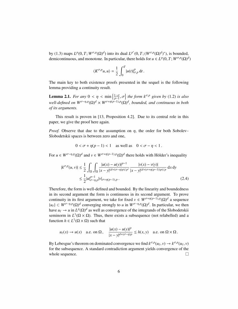
The main key to both existence proofs presented in the sequel is the followinglemma providing a continuity result.

Lemma 2.1. For any 0 < η < min

1−σp−1 , σ

the form kσ,p given by (1.2) is also

well-defined on Wσ−η,p(Ω)d × Wσ+η(p−1),p(Ω)d, bounded, and continuous in bothof its arguments.

This result is proven in [13, Proposition 4.2]. Due to its central role in thispaper, we give the proof here again.

Proof. Observe that due to the assumption on η, the order for both Sobolev–Slobodetskii spaces is between zero and one,

0 < σ + η(p − 1) < 1 as well as 0 < σ − η < 1 .

For u ∈ Wσ−η,p(Ω)d and v ∈ Wσ+η(p−1),p(Ω)d there holds with Holder’s inequality

|kσ,p(u, v)| ≤12

∫Ω

∫Ω

|u(x) − u(y)|p−1

|x − y|(d+(σ−η)p)/p∗|v(x) − v(y)|

|x − y|(d+(σ+η(p−1))p)/p dx dy

≤12|u|p−1σ−η,p|v|σ+η(p−1),p . (2.4)

Therefore, the form is well-defined and bounded. By the linearity and boundednessin its second argument the form is continuous in its second argument. To provecontinuity in its first argument, we take for fixed v ∈ Wσ+η(p−1),p(Ω)d a sequenceu` ⊂ Wσ−η,p(Ω)d converging strongly to u in Wσ−η,p(Ω)d. In particular, we thenhave u` → u in Lp(Ω)d as well as convergence of the integrands of the Slobodetskiiseminorm in L1(Ω × Ω). Thus, there exists a subsequence (not relabelled) and afunction h ∈ L1(Ω ×Ω) such that

u`(x)→ u(x) a.e. on Ω ,|u(x) − u(y)|p

|x − y|d+(σ−η)p ≤ h(x, y) a.e. on Ω ×Ω .

By Lebesgue’s theorem on dominated convergence we find kσ,p(u`, v)→ kσ,p(u`, v)for the subsequence. A standard contradiction argument yields convergence of thewhole sequence.

6

A final observation beforehand is the following known fact about Sobolev–Slobodetskii spaces.

Lemma 2.2. For bounded domains Ω the norm

|||·||| := ‖·‖0,1 + |·|σ,p

is equivalent to ‖·‖σ,p on Wσ,p(Ω)d.

Proof. We first observe that there holds for u ∈ Wσ,p(Ω)d and its integral meanu = vol(Ω)−1

∫Ω

u(x) dx

‖u − u‖p0,p ≤1

vol(Ω)

∫Ω

∫Ω

|u(x) − u(y)|p dx dy ≤diam(Ω)d+σp

vol(Ω)|u|pσ,p .

Hence, by triangle inequality and ‖u‖0,p ≤ c‖u‖0,1 we get that

‖u‖0,p ≤ c(‖u‖0,1 + |u|σ,p

).

On the one hand, we obtain

‖u‖pσ,p = ‖u‖p0,p + |u|pσ,p ≤ c(‖u‖p0,1 + |u|pσ,p

)and hence, there exists c > 0 such that

‖u‖σ,p ≤ c|||u||| .

On the other hand, by Holder’s inequality there follows |||u||| ≤ c‖u‖σ,p.

3. First order evolution problem

In this section, we prove existence and uniqueness of the before-mentioned firstorder problem. Of course, the following result is well-known and can be provenby standard results such as given in the references of Section 1.1. However, wegive an alternative proof which uses the monotonicity only for uniqueness. Thefollowing existence result is based on a particular Galerkin approximation of theunderlying function space Wσ,p(Ω)d combined with compactness methods and thenonlocal structure of Kσ,p.

Theorem 3.1. For u0 ∈ L2(Ω)d, f ∈ L1(0,T ; L2(Ω)d) and g ∈ Lp∗(0,T ; (Wσ,p(Ω)d)∗)there exists a function

u ∈ C([0,T ]; L2(Ω)d) ∩ Lp(0,T ; Wσ,p(Ω)d) ,

u′ ∈ L1(0,T ; L2(Ω)d) + Lp∗(0,T ; (Wσ,p(Ω)d)∗)

7

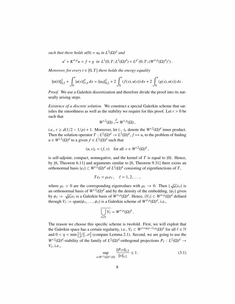
such that there holds u(0) = u0 in L2(Ω)d and

u′ + Kσ,pu = f + g in L1(0,T ; L2(Ω)d) + Lp∗(0,T ; (Wσ,p(Ω)d)∗) .

Moreover, for every t ∈ [0,T ] there holds the energy equality

‖u(t)‖20,2 +

∫ t

0|u(s)|pσ,p ds = ‖u0‖

20,2 + 2

∫ t

0( f (s), u(s)) ds + 2

∫ t

0〈g(s), u(s)〉 ds .

Proof. We use a Galerkin discretization and therefore divide the proof into its nat-urally arising steps.

Existence of a discrete solution. We construct a special Galerkin scheme that sat-isfies the smoothness as well as the stability we require for this proof. Let r > 0 besuch that

Wr,2(Ω)d→ W1,p(Ω) ,

i.e., r ≥ d(1/2 − 1/p) + 1. Moreover, let (·, ·)r denote the Wr,2(Ω)d inner product.Then the solution operator T : L2(Ω)d → L2(Ω)d, f 7→ u, to the problem of findingu ∈ Wr,2(Ω)d to a given f ∈ L2(Ω)d such that

(u, v)r = ( f , v) for all v ∈ Wr,2(Ω)d ,

is self-adjoint, compact, nonnegative, and the kernel of T is equal to 0. Hence,by [6, Theorem 6.11] and arguments similar to [6, Theorem 9.31] there exists anorthonormal basis e` ⊂ Wr,2(Ω)d of L2(Ω)d consisting of eigenfunctions of T ,

Te` = µ`e` , ` = 1, 2, . . . ,

where µ` > 0 are the corresponding eigenvalues with µ` → 0. Then √µ`e` is

an orthonormal basis of Wr,2(Ω)d and by the density of the embedding, ψ` givenby ψ` :=

√µ`e` is a Galerkin basis of Wσ,p(Ω)d. Hence, V` ⊂ Wσ,p(Ω)d defined

through V` := spanψ1, . . . , ψ` is a Galerkin scheme of Wσ,p(Ω)d, i.e.,⋃`∈N

V` = Wσ,p(Ω)d .

The reason we choose this specific scheme is twofold. First, we will exploit thatthe Galerkin space has a certain regularity, i.e., V` ⊂ Wσ+η(p−1),p(Ω)d for all ` ∈ Nand 0 < η < min

1−σp−1 , σ

(compare Lemma 2.1). Second, we are going to use the

Wr,2(Ω)d-stability of the family of L2(Ω)d-orthogonal projections P` : L2(Ω)d →

V`, i.e.,

supv∈Wr,2(Ω)d\0

‖P`v‖r,2‖v‖r,2

≤ 1 . (3.1)

8

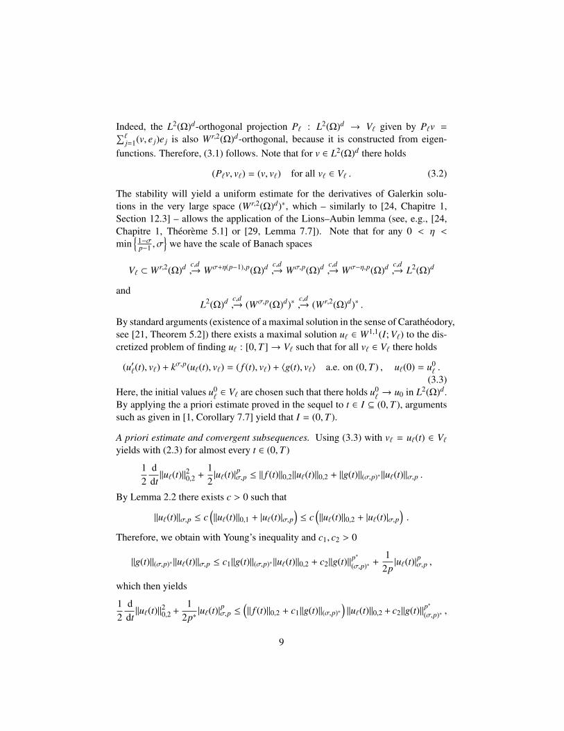
Indeed, the L2(Ω)d-orthogonal projection P` : L2(Ω)d → V` given by P`v =∑`j=1(v, e j)e j is also Wr,2(Ω)d-orthogonal, because it is constructed from eigen-

functions. Therefore, (3.1) follows. Note that for v ∈ L2(Ω)d there holds

(P`v, v`) = (v, v`) for all v` ∈ V` . (3.2)

The stability will yield a uniform estimate for the derivatives of Galerkin solu-tions in the very large space (Wr,2(Ω)d)∗, which – similarly to [24, Chapitre 1,Section 12.3] – allows the application of the Lions–Aubin lemma (see, e.g., [24,Chapitre 1, Theoreme 5.1] or [29, Lemma 7.7]). Note that for any 0 < η <

min

1−σp−1 , σ

we have the scale of Banach spaces

V` ⊂ Wr,2(Ω)d c,d→ Wσ+η(p−1),p(Ω)d c,d

→ Wσ,p(Ω)d c,d→ Wσ−η,p(Ω)d c,d

→ L2(Ω)d

andL2(Ω)d c,d

→ (Wσ,p(Ω)d)∗c,d→ (Wr,2(Ω)d)∗ .

By standard arguments (existence of a maximal solution in the sense of Caratheodory,see [21, Theorem 5.2]) there exists a maximal solution u` ∈ W1,1(I; V`) to the dis-cretized problem of finding u` : [0,T ]→ V` such that for all v` ∈ V` there holds

(u′`(t), v`) + kσ,p(u`(t), v`) = ( f (t), v`) + 〈g(t), v`〉 a.e. on (0,T ) , u`(0) = u0` .

(3.3)Here, the initial values u0

`∈ V` are chosen such that there holds u0

`→ u0 in L2(Ω)d.

By applying the a priori estimate proved in the sequel to t ∈ I ⊆ (0,T ), argumentssuch as given in [1, Corollary 7.7] yield that I = (0,T ).

A priori estimate and convergent subsequences. Using (3.3) with v` = u`(t) ∈ V`yields with (2.3) for almost every t ∈ (0,T )

12

ddt‖u`(t)‖20,2 +

12|u`(t)|

pσ,p ≤ ‖ f (t)‖0,2‖u`(t)‖0,2 + ‖g(t)‖(σ,p)∗‖u`(t)‖σ,p .

By Lemma 2.2 there exists c > 0 such that

‖u`(t)‖σ,p ≤ c(‖u`(t)‖0,1 + |u`(t)|σ,p

)≤ c

(‖u`(t)‖0,2 + |u`(t)|σ,p

).

Therefore, we obtain with Young’s inequality and c1, c2 > 0

‖g(t)‖(σ,p)∗‖u`(t)‖σ,p ≤ c1‖g(t)‖(σ,p)∗‖u`(t)‖0,2 + c2‖g(t)‖p∗

(σ,p)∗ +1

2p|u`(t)|

pσ,p ,

which then yields

12

ddt‖u`(t)‖20,2 +

12p∗|u`(t)|

pσ,p ≤

(‖ f (t)‖0,2 + c1‖g(t)‖(σ,p)∗

)‖u`(t)‖0,2 + c2‖g(t)‖p

∗

(σ,p)∗ ,

9

and, after integrating and multiplying by 2, becomes

‖u`(t)‖20,2 +1p∗

∫ t

0|u`(s)|pσ,p ds ≤ 2

∫ t

0

(‖ f (s)‖0,2 + c1‖g(s)‖(σ,p)∗

)‖u`(s)‖0,2 ds

+ 2c2

∫ t

0‖g(s)‖p

∗

(σ,p)∗ ds + ‖u0`‖

20,2 . (3.4)

Since u` ∈ W1,1(0,T ; V`) ⊂ AC([0,T ]; V`) all terms of the latter inequality arecontinuous and therefore, (3.4) holds for every t ∈ [0,T ]. Moreover, there existst ∈ [0,T ] such that ‖u`(t)‖0,2 = maxt∈[0,T ]‖u`(t)‖0,2. Forgetting about the integral onthe left-hand side of (3.4) we are in the situation to solve the quadratic inequality

‖u`(t)‖20,2 ≤ 2(‖ f ‖L1(0,T ;L2(Ω)d) + c1‖g‖L1(0,T ;(Wσ,p(Ω)d)∗)

)‖u`(t)‖0,2

+ ‖u0`‖

20,2 + 2c2‖g‖

p∗

Lp∗ (0,T ;(Wσ,p(Ω)d)∗).

This yields

‖u`(t)‖0,2 ≤ c(‖ f ‖L1(0,T ;L2(Ω)d) + ‖g‖L1(0,T ;(Wσ,p(Ω)d)∗) + ‖g‖p

∗/2Lp∗ (0,T ;(Wσ,p(Ω)d)∗)

+ ‖u0`‖0,2

).

Since u0`

converges to u0 in L2(Ω)d, the right-hand side of the latter inequality isbounded. Consequently, the right-hand side of (3.4) is bounded and we have forall t ∈ [0,T ]

‖u`(t)‖20,2 +1p∗

∫ t

0|u`(s)|pσ,p ds

≤ c(‖ f ‖2L1(0,T ;L2(Ω)d) + ‖g‖2L1(0,T ;(Wσ,p(Ω)d)∗) + ‖g‖p

∗

Lp∗ (0,T ;(Wσ,p(Ω)d)∗)+ ‖u0

`‖20,2

).

Thus, in view of Lemma 2.2 there exists u ∈ Lp(0,T ; Wσ,p(Ω)d)∩L∞(0,T ; L2(Ω)d)and a subsequence of u`, which will not be relabelled, such that

u`∗ u in L∞(0,T ; L2(Ω)d) , (3.5)

u` u in Lp(0,T ; Wσ,p(Ω)d) . (3.6)

10

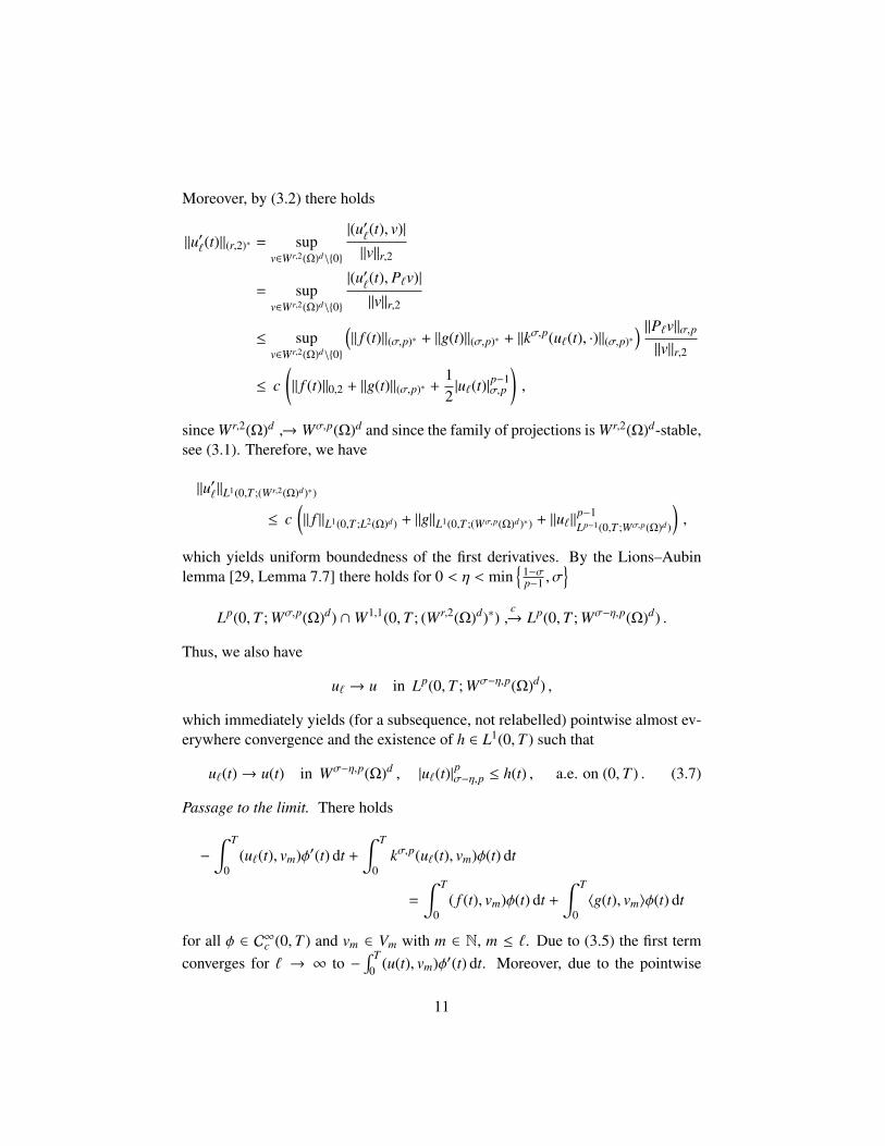
Moreover, by (3.2) there holds

‖u′`(t)‖(r,2)∗ = supv∈Wr,2(Ω)d\0

|(u′`(t), v)|‖v‖r,2

= supv∈Wr,2(Ω)d\0

|(u′`(t), P`v)|‖v‖r,2

≤ supv∈Wr,2(Ω)d\0

(‖ f (t)‖(σ,p)∗ + ‖g(t)‖(σ,p)∗ + ‖kσ,p(u`(t), ·)‖(σ,p)∗

) ‖P`v‖σ,p‖v‖r,2

≤ c(‖ f (t)‖0,2 + ‖g(t)‖(σ,p)∗ +

12|u`(t)|

p−1σ,p

),

since Wr,2(Ω)d → Wσ,p(Ω)d and since the family of projections is Wr,2(Ω)d-stable,see (3.1). Therefore, we have

‖u′`‖L1(0,T ;(Wr,2(Ω)d)∗)

≤ c(‖ f ‖L1(0,T ;L2(Ω)d) + ‖g‖L1(0,T ;(Wσ,p(Ω)d)∗) + ‖u`‖

p−1Lp−1(0,T ;Wσ,p(Ω)d)

),

which yields uniform boundedness of the first derivatives. By the Lions–Aubinlemma [29, Lemma 7.7] there holds for 0 < η < min

1−σp−1 , σ

Lp(0,T ; Wσ,p(Ω)d) ∩W1,1(0,T ; (Wr,2(Ω)d)∗)

c→ Lp(0,T ; Wσ−η,p(Ω)d) .

Thus, we also have

u` → u in Lp(0,T ; Wσ−η,p(Ω)d) ,

which immediately yields (for a subsequence, not relabelled) pointwise almost ev-erywhere convergence and the existence of h ∈ L1(0,T ) such that

u`(t)→ u(t) in Wσ−η,p(Ω)d , |u`(t)|pσ−η,p ≤ h(t) , a.e. on (0,T ) . (3.7)

Passage to the limit. There holds

−

∫ T

0(u`(t), vm)φ′(t) dt +

∫ T

0kσ,p(u`(t), vm)φ(t) dt

=

∫ T

0( f (t), vm)φ(t) dt +

∫ T

0〈g(t), vm〉φ(t) dt

for all φ ∈ C∞c (0,T ) and vm ∈ Vm with m ∈ N, m ≤ `. Due to (3.5) the first termconverges for ` → ∞ to −

∫ T0 (u(t), vm)φ′(t) dt. Moreover, due to the pointwise

11

convergence (3.7), Vm ⊂ Wσ+η,p(Ω)d, and Lemma 2.1, there holds for almost allt ∈ (0,T )

kσ,p(u`(t), vm)→ kσ,p(u(t), vm) .

By the boundedness of kσ,p from Lemma 2.1 and Lebesgue’s theorem on domi-nated convergence in combination with the h ∈ L1(0,T ) from (3.7) we find∫ T

0kσ,p(u`(t), vm)φ(t) dt →

∫ T

0kσ,p(u(t), vm)φ(t) dt .

Therefore, by the limited completeness of the Galerkin scheme we obtain

−

∫ T

0(u(t), v)φ′(t) dt +

∫ T

0kσ,p(u(t), v)φ(t) dt

=

∫ T

0( f (t), v)φ(t) dt +

∫ T

0〈g(t), v〉φ(t) dt

for all φ ∈ C∞c (0,T ) and v ∈ V . Hence, u has a weak derivative and by the densityof C∞c (0,T )⊗Wσ,p(Ω)d in Lp(0,T ; Wσ,p(Ω)d) and the weak∗ density of C∞c (0,T )⊗L2(Ω)d in L∞(0,T ; L2(Ω)d) we arrive at

u′ + Kσ,pu = f + g in L1(0,T ; L2(Ω)d) + Lp∗(0,T ; (Wσ,p(Ω)d)∗) .

It remains to show that u(0) = u0. Observe that since u ∈ Lp(0,T ; Wσ,p(Ω)d) withu′ ∈ L1(0,T ; L2(Ω)d) + Lp∗(0,T ; (Wσ,p(Ω)d)∗) there holds u ∈ C([0,T ]; L2(Ω)d)(this follows from arguments similar to those given in [32, Chapter 20]). On theone hand, since u` ∈ W1,1(0,T ; V`) ⊂ AC([0,T ]; V`) we find for all vm ∈ Vm

−(u0` , vm) =

∫ T

0

[(u`(t), vm)

T − tT

]′dt

=

∫ T

0

(( f (t), vm) + 〈g(t), vm〉 − kσ,p(u`(t), vm)

)T − tT

dt

−1T

∫ T

0(u`(t), vm) dt

and on the other hand, since u ∈ W1,1(0,T ; (Wσ,p(Ω)d)∗) ⊂ AC([0,T ]; (Wσ,p(Ω)d)∗)there holds for all vm ∈ Vm

−(u(0), vm) =

∫ T

0

[(u(t), vm)

T − tT

]′dt

=

∫ T

0

(( f (t), vm) + 〈g(t), vm〉 − kσ,p(u(t), vm)

)T − tT

dt

−1T

∫ T

0(u(t), vm) dt .

12

By the convergences deduced above both right-hand sides coincide for ` → ∞ andby passing to the limit m→ ∞ we obtain u0 = u(0) in L2(Ω)d.

Energy balance. Since we are allowed to test the equation with the solution, thereholds for almost every t ∈ (0,T )

〈u′(t), u(t)〉 + kσ,p(u(t), u(t)) = ( f (t), u(t)) + 〈g(t), u(t)〉 .

Applying the chain rule to the first term, which is valid due to arguments similar tothose given in [32, Chapter 20], and using (2.3) for the second term yields

‖u(t)‖20,2 +

∫ t

0|u(s)|pσ,p ds = ‖u0‖

20,2 + 2

∫ t

0( f (s), u(s)) ds + 2

∫ t

0〈g(s), u(s)〉 ds .

Observe that the proof did not make use of property (2.2). However, if weexploit monotonicity of the nonlinear form, we get uniqueness of the solution.

Theorem 3.2. Under the assumptions of Theorem 3.1 the solution is unique.

Proof. Assume we have two solutions u1 and u2, while u0 and f are fixed. Thenthere holds almost everywhere on (0,T )

〈u′1(t) − u′2(t), v〉 + kσ,p(u1(t), v) − kσ,p(u2(t), v) = 0 for all v ∈ Wσ,p(Ω)d .

Due to the choice of function spaces we are allowed to test with v = u1(t) − u2(t),which yields with (2.2)

ddt‖u1(t) − u2(t)‖20,2 ≤ 0 .

Since u1(0) = u2(0), the solutions coincide (note that u1, u2 ∈ C(0,T ; L2(Ω)d)).

We close this section with a remark on a numerically more suited choice of theGalerkin scheme.

Remark 3.1. From a numerical point of view, the choice of eigenfunctions as aGalerkin basis is disadvantageous. Even though we proved their existence, eigen-functions in general are not given explicitly and it is not known how to constructthem. A more suited Galerkin scheme would be based on finite elements. ThisGalerkin scheme still has to fulfill the smoothness condition (i.e., V` ⊂ Wσ+η(p−1),p(Ω)d,which is usually no problem) and the stability condition on the family of L2(Ω)d-orthogonal projections. Under the additional assumption that Ω ⊂ Rd is polyg-onal, in [5] it is shown that the L2(Ω)-projection onto conforming finite elements

13

(polynomial on each simplex) is stable both with respect to the Lp(Ω)-norm aswell as to the W1,p(Ω)-norm (for the one- and two-dimensional case this resultis also proven in [10]). Hence, by the fundamental property of interpolation the-ory (see, e.g., [26, Theorem B.2] or also [4]), the projection is also stable onWσ,p(Ω) =

[Lp(Ω),W1,p(Ω)

]σ,p

(compare [33, Chapter 34 & 36]). Furthermore,for the Galerkin scheme based on these finite elements the smoothness propertyis directly fulfilled. The drawback, however, is that this result is not known to betrue yet for general Lipschitz domains. Because of that, we chose to work witheigenfunctions.

4. Second order evolution problem

In this section, we develop a setting close to that given in [15]. For this purpose,we consider the space

V := Wσ,p(Ω)d ∩Wγ,q(Ω)d.

Of course, if p = q and σ ≤ γ or the other way around then one space is containedin the other. However, we would like to treat the setting in full generality and do notconsider inclusions. As explained in the introduction, the dual then is determinedas the sum of the duals of the Sobolev–Slobodetskii spaces,

V∗ = (Wσ,p(Ω)d)∗ + (Wγ,q(Ω)d)∗ ,

with norms ‖·‖V = ‖·‖σ,p + ‖·‖γ,q and

‖g‖V∗ = infg=gσ+gγ

gσ∈(Wσ,p(Ω)d)∗

gγ∈(Wγ,q(Ω)d)∗

max‖gσ‖(σ,p)∗ , ‖gγ‖(γ,q)∗

.

We have the scale of Banach spaces

Vd→

Wσ,p(Ω)d

Wγ,q(Ω)d

c,d→ L2(Ω)d c,d

→

(Wσ,p(Ω)d)∗

(Wγ,q(Ω)d)∗

d→ V∗ .

Moreover, we focus on operators Kσ,p : Lp(0,T ; Wσ,p(Ω)d)→ Lp∗(0,T ; (Wσ,p(Ω)d)∗)and Kγ,q : Lq(0,T ; Wγ,q(Ω)d) → Lq∗(0,T ; (Wγ,q(Ω)d)∗) given by (1.2) and (1.3),which share all the properties given in Section 2. Note that in particular there holdsKγ,q : L∞(0,T ; Wγ,q(Ω)d)→ L∞(0,T ; (Wγ,q(Ω)d)∗).

14

Theorem 4.1. For initial values u0 ∈ Wγ,q(Ω)d, v0 ∈ L2(Ω)d and right-hand sidesf ∈ L1(0,T ; L2(Ω)d), g ∈ Lp∗(0,T ; (Wσ,p(Ω)d)∗) there exists a function

u ∈ Cw([0,T ]; Wγ,q(Ω)d) ,

u′ ∈ Lp(0,T ; Wσ,p(Ω)d) ∩ Cw([0,T ]; L2(Ω)d) ,

u′′ ∈ L1(0,T ; L2(Ω)d) + Lp∗(0,T ; (Wσ,p(Ω)d)∗) + L∞(0,T ; (Wγ,q(Ω)d)∗)

with u(0) = u0 and u′(0) = v0 that solves the equation

u′′ + Kσ,pu′ + Kγ,qu = f + g in L1(0,T ; L2(Ω)d) + Lp∗(0,T ; (Wσ,p(Ω)d)∗) .

Moreover, the solution u satisfies for almost every t ∈ (0,T ) the energy estimate

‖u′(t)‖20,2 +

∫ t

0|u′(s)|pσ,p ds +

1q|u(t)|qγ,q

≤ 2∫ t

0( f (s), u′(s)) ds + 2

∫ t

0〈g(s), u′(s)〉 ds + ‖v0‖

20,2 +

1q|u0|

qγ,q .

Proof. Again, we prove this theorem via a Galerkin discretization.

Existence of a discrete solution. Let ψ` be given as in the proof of Theorem 3.1.Then V` ⊂ V with V` = spanψ1, . . . , ψ` is also a Galerkin scheme for V , i.e.,⋃

`∈NV` = V .

In particular, we now have for η and ω chosen appropriately later in the proof that

V` ⊂ Wr,2(Ω)d d→ W1,p(Ω)d c,d

→ Wσ+η(p−1),p(Ω)d ∩Wγ+ω(q−1),q(Ω)d c,d→ V

andV

c,d→ Wσ−η,p(Ω)d ∩Wγ−ω,q(Ω)d c,d

→ L2(Ω)d

as well asL2(Ω)d c,d

→ V∗c,d→ (Wr,2(Ω)d)∗

and the family of L2(Ω)d-orthogonal projections P` : L2(Ω)d → V` is stable withrespect to the Wr,2(Ω)d-norm.

The discretized problem then consists of finding a function u` : [0,T ] → V`such that for all v` ∈ V` there holds

(u′′` (t), v`)+kσ,p(u′`(t), v`)+kγ,q(u`(t), v`) = ( f (t), v`)+〈g(t), v`〉 , t ∈ (0,T ) , (4.1)

with u`(0) = u0`∈ V` and u′`(0) = v0

`∈ V`, for which we assume that u0

`→

u0 in Wγ,q(Ω)d and v0`→ v0 in L2(Ω)d. By standard arguments together with

the subsequent a priori estimate there exists a solution u` ∈ W2,1(0,T ; V`) to thediscretized problem.

15

A priori estimate and convergent subsequences. We test (4.1) with v` = u′`(t) toobtain

12

ddt‖u′`(t)‖

20,2 + kσ,p(u′`(t), u

′`(t)) + kγ,q(u`(t), u′`(t)) = ( f (t), u′`(t)) + 〈g(t), u′`(t)〉 .

Applying Proposition 2.1 there holds kγ,q(u`(t), u′`(t)) = ddt Φ

γ,q(u`(t)) as well askσ,p(u′`(t), u

′`(t)) = 1

2 |u′`(t)|

pσ,p. It follows

‖u′`(t)‖20,2 +

∫ t

0|u′`(s)|pσ,p ds +

1q|u`(t)|

qγ,q

= 2∫ t

0( f (s), u′`(s)) ds + 2

∫ t

0〈g(s), u′`(s)〉 ds + ‖v0

`‖20,2 +

1q|u0` |

qγ,q , (4.2)

and hence

‖u′`(t)‖20,2 +

∫ t

0|u′`(s)|pσ,p ds +

1q|u`(t)|

qγ,q

≤ 2∫ t

0‖ f (s)‖0,2‖u′`(s)‖0,2 ds + 2

∫ t

0‖g(s)‖(σ,p)∗‖u′`(s)‖σ,p ds

+ ‖v0`‖

20,2 +

1q|u0` |

qγ,q .

By Lemma 2.2 and Holder’s inequality there exists c > 0 such that

‖u′`(s)‖σ,p ≤ c(‖u′`(s)‖0,2 + |u′`(s)|σ,p

).

Therefore, we find with Young’s inequality and c1, c2 > 0

‖g(s)‖(σ,p)∗‖u′`(s)‖σ,p ≤ c1‖g(s)‖(σ,p)∗‖u′`(s)‖0,2 + c2‖g(s)‖p∗

(σ,p)∗ +1

2p|u′`(s)|pσ,p ,

which then yields

‖u′`(t)‖20,2 +

1p∗

∫ t

0|u′`(s)|pσ,p ds +

1q|u`(t)|

qγ,q

≤ 2∫ t

0

(‖ f (s)‖0,2 + c1‖g(s)‖(σ,p)∗

)‖u′`(s)‖0,2 ds

+ 2c2

∫ t

0‖g(s)‖p

∗

(σ,p)∗ ds + ‖v0`‖

20,2 +

1q|u0` |

qγ,q . (4.3)

Since u` ∈ W2,1(0,T ; V`) all terms in the latter inequality are continuous andhence, it holds for every t ∈ [0,T ]. In particular, there exists t ∈ [0,T ] such

16

that ‖u′`(t)‖0,2 = maxt∈[0,T ]‖u′`(t)‖0,2. Similarly to the first order setting, we obtainthe quadratic inequality

‖u′`(t)‖20,2 ≤ 2

(‖ f ‖L1(0,T ;L2(Ω)d) + c1‖g‖L1(0,T ;(Wσ,p(Ω)d)∗)

)‖u′`(t)‖0,2

+ 2c2‖g‖p∗

Lp∗ (0,T ;(Wσ,p(Ω)d)∗)+ ‖v0

`‖20,2 +

1q|u0` |

qγ,q ,

which immediately yields

‖u′`(t)‖0,2 ≤ c(‖ f ‖L1(0,T ;L2(Ω)d) + ‖g‖L1(0,T ;(Wσ,p(Ω)d)∗)

+ ‖g‖p∗/2

Lp∗ (0,T ;(Wσ,p(Ω)d)∗)+ ‖v0

`‖0,2 + |u0` |

q/2γ,q

).

Combining this estimate with (4.3) yields for all t ∈ [0,T ]

‖u′`(t)‖20,2 +

1p∗

∫ t

0|u′`(s)|pσ,p ds +

1q|u`(t)|

qγ,q

≤ c(‖ f ‖2L1(0,T ;L2(Ω)d) + ‖g‖2L1(0,T ;(Wσ,p(Ω)d)∗) + ‖g‖p

∗

Lp∗ (0,T ;(Wσ,p(Ω)d)∗)+ ‖v0

`‖20,2 + |u0

` |qγ,q

).

(4.4)

The right-hand side of this inequality is bounded, because v0`

converges to v0 inL2(Ω)d and u0

`converges to u0 in Wγ,q(Ω)d. Note that due to the boundedness of

u′`(t) with respect to |·|σ,p as well as ‖·‖0,2, we obtain boundedness with respectto the full norm ‖·‖σ,p (see Lemma 2.2). Moreover, (4.4) immediately impliesboundedness of u`(t) in L2(Ω)d since

‖u`‖L∞(0,T ;L2(Ω)d) ≤ ‖u0`‖0,2 + T‖u′`‖L∞(0,T ;L2(Ω)d) ,

and the sequence of initial values is bounded. Therefore, the bound of the semi-norm |u`(t)|γ,q implies boundedness of the full norm ‖u`(t)‖γ,q. In view of all thesebounds there exist elements u,w0,wσ and a subsequence, which will not be rela-belled, such that

u`∗ u in L∞(0,T ; Wγ,q(Ω)d) , (4.5)

u′`∗ w0 in L∞(0,T ; L2(Ω)d) , (4.6)

u′` wσ in Lp(0,T ; Wσ,p(Ω)d) . (4.7)

It is clear that u′ = w0 = wσ. In order to pass to the limit in the next step, strongconvergence is needed. Similarly to the first-order setting, the strong convergence

17

we use takes place in a larger space. Now fix 0 < ω < min1−γ

q−1 , γ. Then by the

Lions–Aubin lemma [29, Lemma 7.7] there holds

L∞(0,T ; Wγ,q(Ω)d) ∩W1,∞(0,T ; L2(Ω)d)c→ Lq(0,T ; Wγ−ω,q(Ω)d) .

Thus, by the a priori estimates we gain

u` → u in Lq(0,T ; Wγ−ω,q(Ω)d) ,

and thereforeu`(t)→ u(t) in Wγ−ω,q(Ω)d, a.e. on (0,T ) . (4.8)

Moreover, due to the Wr,2(Ω)d-stability of the orthogonal projection P` : L2(Ω)d →

V` together with its property (u′′` (t), v − P`v) = 0 as well as with the embeddingWr,2(Ω)d → V we find

‖u′′` (t)‖(r,2)∗

= supv∈Wr,2(Ω)d\0

|(u′′` (t), v)|‖v‖r,2

= supv∈Wr,2(Ω)d\0

|(u′′` (t), P`v)|‖v‖r,2

≤ supv∈Wr,2(Ω)d\0

(‖ f (t)‖V∗ + ‖g(t)‖V∗ + ‖kσ,p(u′`(t), ·)‖V∗ + ‖kγ,q(u`(t), ·)‖V∗

) ‖P`v‖V‖v‖r,2

≤ c(‖ f (t)‖0,2 + ‖g(t)‖(σ,p)∗ +

12|u′`(t)|

p−1σ,p +

12|u`(t)|

q−1γ,q

).

Thus, we obtain boundedness of u′′` in L1(0,T ; (Wr,2(Ω)d)∗). Again, by the Lions–Aubin [29, Lemma 7.7] there holds with 0 < η < min

1−σp−1 , σ

fixed

Lp(0,T ; Wσ,p(Ω)d) ∩W1,1(0,T ; (Wr,2(Ω)d)∗)c→ Lp(0,T ; Wσ−η,p(Ω)d) .

Hence, there exists a subsequence (not relabelled) such that

u′` → u′ in Lp(0,T ; Wσ−η,p(Ω)d) ,

and therefore, we obtain pointwise almost everywhere convergence and the exis-tence of h ∈ L1(0,T ) such that

u′`(t)→ u′(t) in Wσ−η,p(Ω)d , |u′`(t)|pσ−η,p ≤ h(t) , a.e. on (0,T ) . (4.9)

18

Passage to the limit. We like to proceed to the limit in the following equation

−

∫ T

0(u′`(t), vm)φ′(t) dt +

∫ T

0kσ,p(u′`(t), vm)φ(t) dt +

∫ T

0kγ,q(u`(t), vm)φ(t) dt

=

∫ T

0( f (t), vm)φ(t) dt +

∫ T

0〈g(t), vm〉φ(t) dt

for all φ ∈ C∞c (0,T ) and vm ∈ Vm with m ∈ N, m ≤ `. The first term convergesdue to (4.6) to −

∫ T0 (u′(t), vm)φ′(t) dt. To get convergence of the second term, we

use (4.9), Vm ⊂ Wσ+η(p−1),p(Ω)d, and Lemma 2.1, which yield kσ,p(u′`(t), vm) →kσ,p(u′(t), vm) for ` → ∞. With Lebesgue’s theorem on dominated convergence incombination with (2.4) from Lemma 2.1 and h ∈ L1(0,T ) from (4.9) we obtain∫ T

0kσ,p(u′`(t), vm)φ(t) dt →

∫ T

0kσ,p(u′(t), vm)φ(t) dt .

For the third term on the left-hand side we copy this strategy. With (4.8), Vm ⊂

Wγ+ω(q−1),q(Ω)d, Lemma 2.1, and Lebesgue’s theorem on dominated convergencein combination with the boundedness of u` in L∞(0,T ; Wγ,q(Ω)d) we have for` → ∞ that ∫ T

0kγ,q(u`(t), vm)φ(t) dt →

∫ T

0kγ,q(u(t), vm)φ(t) dt .

In view of the limited completeness of the Galerkin scheme u solves

−

∫ T

0(u′(t), v)φ′(t) dt +

∫ T

0kσ,p(u′(t), v)φ(t) dt +

∫ T

0kγ,q(u(t), v)φ(t) dt

=

∫ T

0( f (t), v)φ(t) dt +

∫ T

0〈g(t), v〉φ(t) dt

for all φ ∈ C∞c (0,T ) and v ∈ V . This shows that u′ possesses a weak time derivative.Due to the weak∗ density of C∞c (0,T ) ⊗ V in L∞(0,T ; V) we arrive at

u′′ + Kσ,pu′ + Kγ,qu = f + g in L1(0,T ; V∗) .

It remains to show that the initial values are taken. First, we observe that

u` u in W1,2(0,T ; L2(Ω)d) → C([0,T ]; L2(Ω)d) .

Because the trace operator Γ : W1,2(0,T ; L2(Ω)d) → L2(Ω)d, Γv = v(0), is linearand bounded, it is weakly-weakly continuous. Therefore, it follows u0

`= u`(0)

19

u(0). Since u0`→ u0 in Wγ,q(Ω)d, we obtain u(0) = u0. Furthermore, since u′` ∈

W1,1(0,T ; V`) ⊂ AC([0,T ]; V`) there holds on the one hand for all vm ∈ Vm

−(v0` , vm) =

∫ T

0

[(u′`(t), vm)

T − tT

]′dt

=

∫ T

0

(( f (t), vm) + 〈g(t), vm〉 − kσ,p(u′`(t), vm) − kγ,q(u`(t), vm)

)T − tT

dt

−1T

∫ T

0(u′`(t), vm) dt

and on the other hand with u′ ∈ W1,1(0,T ; V∗) ⊂ AC([0,T ]; V∗)

−(u′(0), vm) =

∫ T

0

[(u′(t), vm)

T − tT

]′dt

=

∫ T

0

(( f (t), vm) + 〈g(t), vm〉 − kσ,p(u′(t), vm) − kγ,q(u(t), vm)

)T − tT

dt

−1T

∫ T

0(u′(t), vm) dt .

Hence, with ` → ∞ we obtain (v0, vm) = (u′(0), vm) for all vm ∈ Vm, m ∈ N and bythe limited completeness of the Galerkin scheme u′(0) = v0.

Regularity. By the structure of the equation there holds in particular

u′′ ∈ L1(0,T ; L2(Ω)d) + Lp∗(0,T ; (Wσ,p(Ω)d)∗) + L∞(0,T ; (Wγ,q(Ω)d)∗) .

Furthermore, since u′ ∈ L∞(0,T ; L2(Ω)d) there holds u ∈ L∞(0,T ; Wγ,q(Ω)d) ∩AC([0,T ]; L2(Ω)d) and therefore, we obtain with [25, Chapitre 3, Lemme 8.1] thatu ∈ Cw([0,T ]; Wγ,q(Ω)d). Moreover, since u′′ ∈ L1(0,T ; V∗) there holds u′ ∈L∞(0,T ; L2(Ω)d)∩AC([0,T ]; V∗) and thus, again by [25, Chapitre 3, Lemme 8.1],it follows u′ ∈ Cw([0,T ]; L2(Ω)d).

Energy estimate. Note that we are not allowed to test the equation with the deriva-tive of the solution, because u′(t) is not known to be (almost everywhere) an el-ement of Wγ,q(Ω)d and hence of V . Therefore, we start with the a priori esti-mate (4.2) and obtain due to the weak and weak∗ sequential lower semicontinuityof the norms and seminorms and the convergence of u and the initial values

‖u′(t)‖20,2 +

∫ t

0|u′(s)|pσ,p ds +

1q|u(t)|qγ,q

≤ 2∫ t

0( f (s), u′(s)) ds + 2

∫ t

0〈g(s), u′(s)〉 ds + ‖v0‖

20,2 +

1q|u0|

qγ,q .

20

All the results in this work are also applicable to nonlocal operators that be-have like the fractional p-Laplacian but are not monotone, i.e., they share the samegrowth estimates and the same bounds from below. Such kind of operators arestudied for instance in [13].

References

References

[1] H. Amann, Ordinary Differential Equations: An Introduction to Nonlinear Analysis,De Gruyter, Berlin, 1990.

[2] F. Andreu-Vaillo, J. Mazon, J. Rossi, J. Toledo-Melero, Nonlocal Diffusion Problems,AMS, Providence, Rhode Island, 2010.

[3] V. Barbu, Nonlinear Semigroups and Differential Equations in Banach Spaces, No-ordhoff Int. Publ., Leyden, 1976.

[4] J. Bergh, J. Lofstrom, Interpolation Spaces, Springer, Berlin, 1976.

[5] M. Boman, Estimates for the L2-projection onto continuous finite element spaces ina weighted Lp-norm, BIT Numer Math 46 (2006) 249–260.

[6] H. Brezis, Functional Analysis, Sobolev Spaces and Partial Differential Equations,Springer, 2011.

[7] M. Bulıcek, J. Malek, K. Rajagopal, On Kelvin–Voigt model and its generalizations,Evol. Equations Control Theory 1 (2012) 17–42.

[8] X. Cabre, Y. Sire, Nonlinear equations for fractional Laplacians I: Regularity, maxi-mum principles, and Hamiltonian estimates, Ann. I. H. Poincare 31 (2014) 23–53.

[9] X. Cabre, Y. Sire, Nonlinear equations for fractional Laplacians II: Existence, unique-ness, and qualitative properties of solutions, Trans. Amer. Math. Soc. 367 (2015)911–941.

[10] M. Crouzeix, V. Thomee, The stability in Lp and W1p of the L2-projection onto finite

element function spaces, Math. Comp. 48 (1987) 521–532.

[11] S. Demoulini, Weak solutions for a class of nonlinear systems of viscoelasticity,Arch. Rational Mech. Anal. 155 (2000) 299–334.

[12] E. Emmrich, R. B. Lehoucq, D. Puhst, Peridynamics: a nonlocal continuum theory,in: M. Griebel, M. A. Schweitzer (eds.), Meshfree Methods for Partial DifferentialEquations VI, Lect. N. Comput. Sci. Engin., vol. 89, Springer, Berlin, 2013, pp. 45–65.

21

[13] E. Emmrich, D. Puhst, Measure-valued and weak solutions to the nonlinear peridy-namic model in nonlocal elastodynamics, Nonlinearity 28 (2015) 285–307.

[14] E. Emmrich, M. Thalhammer, Doubly nonlinear evolution equations of second order:Existence and fully discrete approximation, J. Differential Eqs. 251 (2011) 82–118.

[15] E. Emmrich, D. Siska, Evolution equations of second order with nonconvex potentialand linear damping: existence via convergence of a full discretization, J. DifferentialEqs. 255 (2013) 3719–3746.

[16] H. Engler, Global regular solutions for the dynamic antiplane shear problem in non-linear viscoelasticity, Math. Z. 202 (1989) 251–259.

[17] A. Friedmann, J. Necas, Systems of nonlinear wave equations with nonlinear viscos-ity, Pacific J. Math. 135 (1988) 29–55.

[18] G. Friesecke, G. Dolzmann, Implicit time discretization and global convergence fora quasi-linear evolution equation with nonconvex energy, SIAM J. Math. Anal. 28(1997) 363–380.

[19] H. Gajewski, K. Groger, K. Zacharias, Nichtlineare Operatorgleichungen undOperatordifferentialgleichungen, Akademie-Verlag, Berlin, 1974.

[20] Q.-Y. Guan, Z.-M. Ma, Boundary problems for fractional Laplacians, Stoch. Dyn. 5(2005) 385–424.

[21] J. Hale, Ordinary Differential Equations, Robert E. Krieger Publ. Comp., New York,1980.

[22] T. Kobayashi, H. Pecher, Y. Shibata, On a global in time existence theorem of smoothsolutions to a nonlinear wave equation with viscosity, Math. Ann. 296 (1993) 215–234.

[23] N. S. Landkof, Foundations of Modern Potential Theory, vol. 180 of GrundlehrenMath. Wiss., Springer, Berlin, 1972.

[24] J. L. Lions, Quelques methodes de resolution des problemes aux limites non lineaires,Dunod, Paris, 1969.

[25] J. L. Lions, E. Magenes, Problemes aux limites non homogenes et applications, vol. 1,Dunod, Paris, 1968.

[26] W. McLean, Strongly Elliptic Systems and Boundary Integral Equations, CambridgeUniversity Press, Cambridge, 2000.

[27] E. Di Nezza, G. Palatucci, E. Valdinoci, Hitchhikers guide to the fractional Sobolevspaces, Bull. Sci. Math. 136 (2012) 521–573.

22

[28] A. Prohl, Convergence of a finite element based space-time discretization in elasto-dynamics, SIAM J. Numer. Anal. 46 (2008) 2469–2483.

[29] T. Roubıcek, Nonlinear Partial Differential Equations with Applications, 2nd ed.,Birkhauser, Basel, 2013.

[30] S. A. Silling, Reformulation of elasticity theory for discontinuities and long-rangeforces, J. Mech. Phys. Solids 48 (2000) 175–209.

[31] E. Stein, Singular Integrals and Differentiability Properties of Functions, PrincetonUniversity Press, Princeton, New Jersey, 1970.

[32] L. Tartar, An Introduction to Navier–Stokes Equation and Oceanography,Lect. N. UMI 1, Springer, Berlin, 2006.

[33] L. Tartar, An Introduction to Sobolev Spaces and Interpolation Spaces, Lect. N.UMI 3, Springer, Berlin, 2007.

[34] J. L. Vazquez, Nonlinear diffusion with fractional Laplacian operators, in: H. Holden,K. H. Karlsen (eds.), Nonlinear Partial Differential Equations, The Abel Symposium2010, Springer, Berlin, 2012, pp. 271–298.

[35] J. Wloka, Partial differential equations, Cambridge University Press, Cambridge,1987.

[36] E. Zeidler, Nonlinear Functional Analysis and its Applications II/B, Springer, NewYork, 1990.

23