On the Evolution of the Firm Size Distribution

in an African Economy 1

Justin Sandefur2

Abstract

The size of the informal sector is commonly associated with low per capitaGDP and a poor business environment. Recent episodes of reform and growthin several African countries appear to contradict this pattern. From the mid1980’s onward, Ghana underwent dramatic liberalization and achieved steadygrowth, yet average firm size in the manufacturing sector fell from 19 to just9 employees between 1987 and 2003. I use a new panel of Ghanaian firms,spanning 17 years immediately post-reform, to model firm dynamics thatdiffer markedly from well-established ‘stylized facts’ in the empirical literaturefrom other regions. In contrast with American and European firms, entry ofnew firms and selection on observable characteristics, rather than within-firmgrowth, dominates industrial evolution in Ghana.

1. Introduction

The size of the informal sector is commonly associated with low per capita GDP anda poor business environment. Market deregulation (Besley and Burgess, 2004; Botero,Djankov, La Porta, Lopez de Silanes, and Shleifer, 2004; de Soto, 1989), enforcement ofproperty rights (Beck, Demirguc-Kunt, and Levine, 2003; Kumar, Rajan, and Zingales,

1I am grateful to Professor Nicholas Nuamah and Tony Krakah of the Ghana Statistical Service (GSS)for their assistance accessing the National Industrial Census; Moses Awoonor-Williams for organizingvarious aspects of the survey data collection; Luis Cabral and Jose Mata for assistance reproducing theirearlier results; Ernest Aryeetey, Chris Woodruff and seminar participants at the IZA/WB Conferenceon Employment and Development for comments; and to my supervisor Francis Teal for consistent input.This document is an output of research funding from the UK Department for International Development(DFID) as part of the iiG, a research programme to study how to improve institutions for pro-poorgrowth in Africa and South-Asia. The views expressed are not necessarily those of DFID.

2Centre for the Study of African Economies, Dept. of Economics, Oxford University. Tel. +44 (0)1865284 787, justin.sandefur@economics.ox.ac.uk.

1

CSAE WPS/2010-05

1999), and low rates of taxation and bribe extraction are commonly thought to contributeto the emergence of larger, formal enterprises.

The recent track record of several African economies calls these patterns into ques-tion. Beginning in the mid 1980s, Ghana launched one of the most ambitious structuraladjustment programs in Africa, abolishing price controls, opening capital markets, slash-ing tariffs, and eventually privatizing the majority of state owned enterprises. Thesereforms ushered in a period of sustained economic growth, averaging 4.7% per annumfrom 1984 to 2004 (Aryeetey and McKay, 2007). Yet, as I attempt to document below,over this same period Ghana saw a rapid increase in the relative size of the informalsector, and a secular decline in the average size of industrial activity. Furthermore, thispattern seems to be common across sub-Saharan Africa. During the 1990s, all of theeconomies for which comparable employment data is available (Cote d’Ivoire, Ghana,Uganda, Kenya and Tanzania) posted slow but positive growth in per capita GDP, andall underwent substantial market-oriented reforms in the 1980s and early 1990s. Nev-ertheless, all of these economies saw substantial increases in the proportion of the non-agricultural labor force working in the small-scale or informal sector (Kingdon, Sandefur,and Teal, 2006).

This paper uses data from the manufacturing sector in Ghana to investigate thedeterminants of this trend in detail. I study the evolution of the firm size distributionin Ghana from 1987 to 2003. The main contribution of the paper is to establish twosignificant departures from well-documented, international ‘stylized facts’. Both of thesedepartures highlight the overwhelming importance of firm entry and selection, and theirrelevance of within-firm growth, in understanding industrial evolution in Ghana. Incontrast, much previous research on firm dynamics in Africa, by focusing primarily oncross-sections or tracking a fixed panel of existing firms, has systematically overlooked theunique patterns of firm entry and selection that appear to distinguish Africa’s industrialdevelopment.3

Seen in isolation, the recent influx of microenterprises in Ghana could be viewedas either the harbinger of future industrial dynamism, or a sign that formal sector is inrelative decline. The firm dynamics documented here provide little basis for optimism.Based on existing patterns of firm growth and survival, there is no sign that currentcohorts of new firms contain the seeds of future large-scale enterprises.

The rest of the paper is organized as follows. The next section presents the twoprimary data sources used in the analysis: two rounds of an industrial census and a

3The firm-level panel studies funded by the World Bank through the Regional Program on EnterpriseDevelopment (RPED), and subsequent cross-sectional Investment Climate Assessment (ICA) surveys areprime examples of frequently-used data sets that have contributed to this blindspot regarding firm entry.Notable exceptions include recent work on Ethiopia, using firm census data (Shiferaw and Bedi, 2009).

2

12-year panel survey of a sample of firms. Section 3 relies on graphical analysis todocument the first significant finding of the paper: the dominance of selection overwithin firm growth in explaining the apparent life-cycle of firms, counter to existingevidence from Europe and elsewhere. Section 4 models the distribution dynamics inGhanaian manufacturing using a simple, first-order, homogenous Markov chain. TheMarkov model allows me to recover entry rates, and to place overall patterns of jobcreation and reallocation in a comparative international context. Section 5 turns to theunderlying determinants of this trend toward small-scale employment, and the apparentfailure of the common association between liberalization and large scale development. Itest the importance of credit constraints in explaining the low rates of firm growth atvarious points in the size distribution. Results suggest that credit market failures placea significant drag on growth among small firms, but the relaxation of all such constraintswould be insufficient to overcome the leftward shift in Ghana’s firm size distribution.Section 6 concludes.

2. Data

The analysis draws on two primary data sources: (i) two waves of Ghana’s Na-tional Industrial Census (NIC) – spanning nearly two decades in the immediate wake ofliberalization, 1987 and 2003 – and (ii) longitudinal survey data from a sub-sample ofthe 1987 NIC firms, tracking them from 1991 to 2002.

2.1. Census data

The remarkable feature of the NIC data is the dramatic fall in average firm sizebetween the two rounds of the census, indicating a steep trend toward smaller scaleactivity.

The second and third rounds of the census were undertaken by the Ghana StatisticsOffice (GSO) in 1987 and 2003, respectively, both with the collaboration of the UnitedNations Industrial Development Organization (UNIDO). Comprehensive coverage andsynchronized variable definitions across the two censuses allow for comparisons acrossyears. The NIC incorporates all manufacturing firms in the country, spanning both theformal and informal sector. Household enterprises are excluded, except in cases wherepublic signs clearly advertise the location of a business enterprise within a residentialdwelling. The NIC is enumerated at the plant level, thus multi-plant firms are treated asseparate observations. As such multi-plant firms are likely to be quite rare in Ghana, par-ticularly in the private sector, I use the terms plant and firm interchangeably throughout.At the time of writing, the available variables which are common across census rounds areextremely limited. They include the establishment name, location (region and town),and 4-digit International Standard Industrial Classification (ISIC) codes, and persons

3

engaged. Persons engaged includes both employees and unpaid apprentices which con-stitute a significant share of the small-enterprise workforce. Additionally, in 2003 firmage is also available, which is central to reconstructing historical entry rates in section4.4

As seen in Table 1, the firm size distribution in Ghanaian manufacturing shiftedsignificantly downward between 1987 and 2003. Average firm size fell from 19 to 9employees per establishment, while the proportion of employment in small and microen-terprises (fewer than 30 employees) rose from 33% to 52%.

There is strong evidence this change is genuine, rather than being driven by anychange in the coverage of the census between rounds. At least three pieces of evidencecorroborate the overall pattern of a large reduction in average firms size. First, as canbe seen in Table 1, the downward shift in the size distribution occurred across all sizecategories. Removing firms with fewer than 10 or fewer than 20 employees – where onemight speculate coverage has improved – does not alter the picture of declining firm size.

Second, the NIC figures on employment in the manufacturing sector for 1987 and2003 closely match the equivalent numbers from the population censuses conducted in1984 and 2000. As seen in Table 2, the NIC reports 157,084 and 243,516 employees in 1987and 2003, respectively, while the population census records 137,119 and 229,156 wageemployees and apprentices in the manufacturing sector in 1984 and 2000, respectively –which rises to 150,708 and 251,866 after adjusting for trend growth in the three year gapbetween the population census and NIC. This relatively small discrepancy of just 3 to4% would make it seem highly improbably that there was severe under-counting in the1987 NIC. Furthermore, the dramatic expansion in apprenticeship labor – 7.1% annualgrowth compared to 1.8% for the labor force as a whole, in an occupational categoryusually restricted to small, Ghanaian-owned, informal enterprises, and generally unpaid– is another indication of increasing informality.

Third, the shift in the firm size distribution is also corroborated by another in-dependent data source: the Ghana Living Standards Surveys (GLSS I-IV), a series oflarge-scale, household socio-economic surveys conducted in 1987/88, 1988/89, 1991/92and 1998/99. Kingdon, Sandefur and Teal Kingdon, Sandefur, and Teal (2006) presenta picture of the evolution of the urban labor market in Ghana by linking these foursurveys, tracking the share of the labor force in public versus private sector wage em-ployment, unemployment and self employment. Between GLSS I (1987/88) and GLSSIV (1998/99), the share of the urban labor force in self-employment rose from 50% to

4Data from the 1987 NIC is coded according to Revision 2 of the ISIC, while the 2003 NIC uses ISICRevision 3, as does the survey data presented in the next section. Because there is no precise translationof three- and four-digit ISIC codes between revisions – short of reclassifying individual firms – analysisis restricted to two digit classification, yielding a total of 17 industries.

4

63%, while private wage employment grew only slightly and the public sector contracted.Thus the broad picture of increasing informality and a trend toward small-scale activityis consistent across all available, nationally representative data sets.

2.2. Survey data

The Ghana Manufacturing Enterprise Survey (GMES) collected data on a sampleof firms over a period from 1992 to 2002. The surveys were conducted by a team fromthe Centre for the Study of African Economies, Oxford, the University of Ghana, Legon,and the Ghana Statistical Office (GSO), Accra. The surveys from 1992 to 1994 were partof the Regional Program on Enterprise Development (RPED) organized by the WorldBank, enabling comparison with similar surveys conducted in other Africa countries overthe same period.

The original GMES sample of 200 firms was initially drawn from the 1987 NIC,spanning 10 two-digit ISIC sectors and oversampling larger firms with more than 100employees. The survey includes a full production and input data, firm-specific input andoutput prices, measures of the human capital of workers and management, questions onaccess to finance, taxes and the regulatory environment, etc. Firms were surveyed up toseven times (in 1992, ‘93, ‘94, ‘96, ‘98, 2000 and 2003) with recall data collected for theintervening years. As firms exited they were replaced with new respondents, creating anunbalanced panel covering a total of 312 firms for up to 12 consecutive years, 1991-2002.The mean and median number of observations per firm are 6.98 and 7, respectively.

Large and small firms in the survey data use strikingly different factor intensities,have different propensities to export, pay different prices for both capital and labor, andface different regulatory environments. These systematic differences provide hints aboutboth the causes and consequences of the shift in the firm size distribution shown above.

As seen in Table 3, larger firms pay substantially higher wages for workers withsimilar characteristics. Median monthly wages range from US$ 24.08 for firms with fewerthan five employees up to US$ 125.87 for firms with over 100 workers. While a portionof this difference is undoubtedly attributable to higher skilled labor usage among largefirms, previous studies have found that the remaining firm-size wage effect for workerswith similar characteristics is still extremely large. Based on earnings equations estimatedfor the sector by Soderbom & Teal Soderbom and Teal (2004), a firm with 100 employeeswill pay roughly double the wage of a firm with 10 employees, controlling for workers’observed and time-invariant unobserved skills.

While large firms pay more for labor, there is evidence that they pay significantlyless for credit. A simple way to capture these differences without resorting to econometricestimation is to measure the implied return to capital for each firm using data on profitsand the capital stock (Bigsten, Collier, Dercon, Fafchamps, Gauthier, Gunning, Isaksson,

5

Oduro, Oostendorp, Pattillo, Soderbom, Teal, and Zeufack, 2003). In a competitiveindustry the following zero-profit condition

πit = ptqit − witXit − ritKit = 0

provides a solution for the firm-specific interest rate,

rit =ptqit − witXit

Kit

where p is the product price, q is real output, w is a firm specific vector of input prices,K measures the capital stock and X is a vector of other factor inputs, including labor.Table 3 reports this measure of r for firms in each size class. Applying the zero profitcondition to firms in our sample implies that medium firms must pay an effective interestrate of 58% on capital, compared to an astronomical 1,623% for microenterprises.

Finally, a more direct way to assess credit constraints among firms is simply toask their managers. The bottom of Table 3 reports data from managers’ responses tothe question “What are your three biggest problems this year?”5 The responses acrosslarge- and small-firm managers conform to a picture of widespread credit constraintsin the informal sector. Credit access is listed as a major problem by nearly 70% ofmicroenterprises and only 20% of large firms. Meanwhile, large firms are eight-timesmore likely to complain of interest rates, implying that credit is available for a sufficientcost. These self-reported measures of credit access are employed in the estimation offirm growth model in section 5, where I deal explicitly with the problems of endogeneityand measurement error that such self-reported data poses.

3. Graphical Analysis: Growth vs. Selection

One of the main stylized facts to emerge from the recent empirical literature onindustrial evolution in developed economies is the existence of clear life cycle amongfirms: entering cohorts are relatively small and in their early years firms either convergefairly quickly to their long-run size or die (Sutton, 1997). The 2003 Census provides dataon firm age, which I divide into the following categories: younger than 1 year, 2-4, 5-9,10-19, 20-29, and 30 years or older. Figure 1 plots nonparametric estimates of the firmsize distribution in logs by age category using the cross-section of firms in 2003 Census.6

5Respondents were not prompted or given a list of options. Enumerators coded the replies into oneof twenty-six categories ex post. The data in Table 3 and the variables used in section 5 are dummyvariables taking a value of one if a given issue was listed as either the first, second, or third largestproblem.

6Plots are based on an Epanechnikov kernel density smoother. For comparability, all plots use abandwidth of 1.

6

Consistent with the life-cycle pattern, older firms are consistently larger than those inlater cohorts.

However, there is an inherent ambiguity in the patterns observed in Figure 1. Usingonly a cross-section of firms, it is impossible to distinguish the hypothesis that youngerfirms grow quickly from the alternative hypothesis of selection: small firms die morefrequently and thus average size within a cohort increases as it ages.

Cabral and Mata Cabral and Mata (2003) demonstrate a simple graphical methodof distinguishing growth from selection in panel data. Their technique is to comparethree distinct firm size distributions at two points in time: the period 1 distribution ofall firms; the period 2 distribution of firms which survived between rounds; and finally,with the benefit of hindsight, the period 1 distribution of firms which are known to havesurvived to period 2.

Figure 2 replicates the test suggested by Cabral and Mata using the Ghana Indus-trial Census data. 7 The curve with the highest peak shows the distribution of all firms in1987/88. The remaining curves plot the size distribution of firms which survived betweenperiods, in both the initial round (1988S) and sixteen years later (2003). The relativeposition of these last two curves provides a simple test of the selection hypothesis: didfirms which survived grow during the interim, or were they large to begin with?

The results show that the evolution of firm size over the life cycle is driven almostentirely by selection in Ghana. Rather than starting as a representative sample of thepopulation and growing over time, the Ghanaian firms which survived from 1987 to 2003had negative average growth. The rightward shift in the distribution over time is entirelydue to the fact that surviving firms were abnormally large to begin with. 8

For comparison, I reproduce the analogous figures from Cabral and Mata 2003, p.1079 in the left panel of figure 2. The distributions are based on data from Portuguesemanufacturing firms, which Cabral and Mata argue are fairly representative of developedcountry data sets in terms of their size distribution and evolution. As in Ghana, olderfirms are bigger in the Portuguese data. As seen in the figure 2 however, the pattern ofgrowth and selection in this sample is almost precisely the opposite of that observed inGhana. The figure shows that for Portuguese manufacturing firms, selection (by size)

7Unfortunately, firm age is not reported in the 1987 census, so I am unable to identify the 1987 cohortof entrants. Instead, I trace the evolution of the 1987 population of firms over time. An additionaldifficulty is encountered in matching firms between the two rounds of the census, as no unique identifieris provided. In the end, I were able to match 236 firms by ISIC code, region, and firm name.

8It is important to note that the panel of 305 survivors which I identify represents only about 13%of the firms in the 2003 census which claimed to have entered in 1988 or earlier. Comparing these 305to the larger population of alleged survivors, average firm size is somewhat larger for those I was able tomatch. However, this will undermine our conclusion in the text only if these 305 firms grew significantlymore slowly than the average for the population of survivors. As shown above, there is no evidence oflarge discrepancies between size classes in within-firm growth rates in Ghana.

7

plays a very small role in the evolution of the firm size distribution. Cabral and Mataargue that this finding calls for a reevaluation of the central role given to selection inmuch of the theoretical literature on industrial evolution, notably Jovanovic Jovanovic(1982).

These contrasting findings have enormous implications for how one views the bur-geoning SME sector in Ghana. Were the same explosion of entrepreneurial activity takingplace in Portugal, there would be reason to believe that the influx of new firms containedthe seeds of future large scale industrial development. Such is not the case in Ghana.Existing evidence suggests that small enterprises die early and small. Conversely, bigfirms don’t represent successful microentrepreneurs that have risen through the ranks ofsmaller firms. Rather, big firms are born big.

4. Distribution Dynamics

I model the evolution in the distribution of firm size from 1987 to 2003, whichI denote F1987 and F2003 respectively, using a first-order, homogenous Markov chain.The central conceit of the Markov framework is that a firm’s fate tomorrow (i.e., itssize, or continued existence) depends only on its status today, with no further role forhistory. While this assumption may be questioned in high-frequency data, in transitionsover longer time spans – such as the 16 years used here – growth trajectories will likelyoverwhelm any bias due to serial correlation in the data (Davis, Haltiwanger, and Schuh,1996).

There are two main objectives to this modelling exercise. First, I use the transitionand exit matrices from the Markov model to reconstruct entry rates and thus measuregross job flows at various points in the distribution. Second, by allowing for more generaldynamics than in a linear growth model, I can remain agnostic about the shape of theergodic distribution of firm size. This allows me to test hypotheses such as those putforward by Quah Quah (1997), who finds that the distribution of per capita incomesacross countries appears to be converging to a bimodal distribution, or common claimsthat African firms exhibit a ‘missing middle’.

The Markov model contains three basic sets of parameters: (i) entry rates of newfirms, (ii) transition probabilities between size classes for firms that survive from oneperiod to the next, and (iii) exit rates. The latter two categories, transition and exitprobabilities, can be estimated fairly directly from the data – and as a result havebeen analyzed quite extensively by previous studies – while entry rates must be inferredsomewhat indirectly. This task of inferring entry rates is the main analytical challenge inestimating a Markov model for Ghanaian firms. As I hope to show, however, firm entrypatterns are also the most notable and economically significant component of Ghana’srecent industrial development.

8

The census data distinguish nine size categories, allowing me to represent the dis-tribution of firm sizes as a vector of nine discrete densities, which I refer to as Ft. Thedistribution in year t is linked to the distribution in the following year by a 9× 9 matrixof transition probabilities:

F2003 = M16F1987

= (B + S′D)16F1987,(1)

where subscripts denote the year of observation and superscripts are exponents denotingthe powers of a matrix. The second line decomposes the shift in the distribution into avector of firm entry or “birth” rates B, a matrix of transition probabilities conditionalupon survival, S, and a vector of firm exit or “death” rates, D:

B =

⎛⎜⎜⎝

b1 0. . .

0 b9

⎞⎟⎟⎠ , S =

⎛⎜⎜⎝

s11 . . . s19

.... . .

...s91 . . . s99

⎞⎟⎟⎠ , D =

⎛⎜⎜⎝

1 − d1 0. . .

0 1 − d9

⎞⎟⎟⎠

The parameters bi and di are birth or death rates, respectively, defined as the number offirms entering or exiting a given size class between two periods as a proportion of thoseobserved in initial period. Element sij of the S matrix denotes the probability that afirm starting in size class i will transition to class j. Because the S matrix maps thedistribution of surviving firms from one period to the next, its rows must sum to one.This is not the case with the combined M matrix, however, which will incorporate entryand exit rates.9

4.1. Transition matrices

I use the panel of firms in both the NIC and GMES data to estimate the S matrix,or the probability that firm i beginning in size category p ends up in size category q.Using a multinomial logit form, this probability is expressed as a function of nine dummy

9It may not be obvious at first glance why the decomposition in line (1) is additive with respect toentry rates and multiplicative with respect to exit rates. Multiplying through the expression element byelement yields the following solution for the final density:

Ft =

⎛⎜⎝

ft,1

...ft,9

⎞⎟⎠ =

⎛⎜⎝

b1ft−1,1 +∑9

i=1 si1dift−1,i

...

b9ft−1,9 +∑9

i=1 si9dift−1,i

⎞⎟⎠

This expression is arguably more intuitive: the number of firms observed in class 1 in period t is equalto the new entrants in that class (b1ft−1,1) plus the sum of all firms moving into or remaining in class 1.Because transition probabilities are estimated conditional on firm survival, exit rates must be multipliedby the original density before allowing for firm growth.

9

variables corresponding to each of the firm size classes:

spq =exp(βqI(ni,t−1 ∈ p))

1 +∑

q exp(βqI(ni,t−1 ∈ p))(2)

where I(.) is the indicator function, taking a value of one if ni,t−1 falls in size class p

and zero otherwise. These probabilities, spq, correspond to the individual elements ofthe transition matrix, S.10

One advantage of the multinomial logit model for this problem is that it imposes therestriction that all probabilities sum to one. The Markov model also suggests additionalconstraints which can be imposed on the β parameters. It is intuitively clear that thetrue S matrix should map the original 1987 firm size distribution to the distribution ofsurviving firms in 2003. However, there is no guarantee that straightforward multimoniallogit estimates of S will satisfy this condition. This is because estimation of (2) reliesonly on data from the sample of 305 firms that can be tracked across both rounds ofthe census. To put this more formally, let F s

2003,t denote the distribution of firms bornin period t and observed in 2003, i.e., the distribution of survivors from the period t

cohort. This distribution of survivors should reflect the cumulative transitions and exitsoccuring since period t, such that

F s2003,≤1987 = (S′D)16F1987. (3)

To improve the fit of the model, it is possible to impose (3) as a constraint on thelikelihood maximization used to estimate (2).11

Table 6 presents estimates of the 16-year transition matrix based on the NIC, using

10Ideally, these probabilities could be estimated for every point on a continuous distribution using, forinstance, a stochastic kernel estimator as advocated by Quah Quah (1997). Such an approach avoids theneed to impose an arbitrary discretization on the distribution, as this may effect the dynamics of theMarkov chain. In the present application, however, the nine discrete size categories used in the analysiswere dictated by the available data.

11The system of equations in 3 is clearly non-linear with respect to βq. I rely on a linear approximationof these constraints to enable me to implement them with the constraint option on the standard mlogitcommand in STATA. In keeping with the earlier notation, let fs

q,2003,≤1987 be the qth individual elementof the F s

2003,≤1987 distribution, i.e., the number of firms born in or before 1987 and observed in 2003 insize class q. Then the system of constraints in (3) can be written as:

fsq,2003 =

9∑p=1

spqdpfp,1987 for q = 1, 2, . . . , 9.

Substituting 2 into 3 yields

fsq,2003 =

9∑p=1

exp(βqI(ni,t−1 ∈ p))

1 +∑

q exp(βqI(ni,t−1 ∈ p))dpfp,1987.

The first order Taylor-series approximation of exp(βq) around βq = 0 is simply 1 + βq. However, I aminterested in an approximation to βq around its true value, which may be far from zero. To circumventthis problem, I assume that the unconstrained estimate of βq is a reasonably close approximation of the

10

the sample of firms that were tracked between rounds. Starting sizes are listed along theleft hand side and ending sizes are listed on the top of the matrix. Blank spaces representzero probabilitiy events. If the distribution is completely stable, all mass should be foundon the diagonal.

There are several notable features about the figures in the table. First, the modestaverage net growth rates observed in the previous section belie a high level of churning inthe firm size distribution and considerable heterogeneity in growth rates. Firms beginningin the middle size ranges fan out to virtually all points in the distribution over 16 years.Second, in the jargon of Markov analysis, the system is said to communicate acrossthe entire distribution. This simply means that all size classes are, in a probabilisticsense, achievable from any given starting point over a sufficiently long span of time (i.e.,repeated iterations of the matrix). It is significant to point out, however, that evenover the fairly long time span used here, there are no observed cases of microenterprisesmaturing into large scale employers. Third, the bottom row of the table presents theergodic distribution implied by the transition matrix. Assuming infinite lives for all firms,there is evidence of an emerging bimodal distribution among Ghanaian firms. While theactual realization of this distribution is prevented by firm death, this pattern is furtherevidence that small and large firms should be understood as fundamentally different,rather than simply occupying different points in a life-cycle trajectory.

4.2. Exit rates and the selection process

What role did firm exit play in the evolution of the firm size distribution in Ghanafrom 1987 to 2003? Even if growth and entry rates were identical across size classes,the shift in the firm size distribution over this period may have occurred simply dueto accelerated death rates at the upper end of the distribution. The economic reformsof the 1980s may have had a particularly harsh effect on large enterprises (Appiah-Kubi, 2001; Asante, Nixson, and Tsikata, 2000). Liberalization brought the end of manypolicies – such as subsidized credit schemes, priority access to foreign exchange, and dejure product market monopolies – which had previously benefit large firms. Thus, as asimple descriptive statistic, it is informative to compare exit rates across size classes. Inaddition, these rates are a necessary ingredient in calculating transition and entry ratesin the following sections.

true parameter. This allows me to write

exp(βq) = exp(βq)exp(βq − βq) ≈ exp(βq)(1 + βq − βq),

which I use to linearize the system of constraints in (3). Once linearized the constraints can be imple-mented with standard software packages. Estimation proceeds in two stages. In the first stage estimatesof βq are obtained from unconstrained estimation of (2). These estimates are then used to linearize (3)and the multinomial model is re-estimated with the approximated constraints.

11

I compute firm exit rates, or the parameters of the D matrix, using the GMESsample. The GMES data set is well-suited for measuring exit rates as it contains anindicator variable which distinguishes genuine firm exits from other forms of sampleattrition, e.g., manager’s refusal to participated in the survey in subsequent rounds,enumerator’s inability to locate a micro-entrepreneur who may have relocated his or herbusiness, etc. Such information is not available in the census. Using this variable, Iestimate probit model of firm exit where the right hand side variables include dummiesfor each size class and, in some specifications, controls for location, firm age and year ofthe survey. The exit probit is estimated over two year intervals, using data from 1991,1993, 1995, 1997 and 1999.12 Intermediate rounds are based on recall data and thus, byconstruction, it is impossible to observe exits in these periods. Size classes are defined inone of two ways: using firm employment in the final survey round prior to employment,or using average employment for all rounds in which data are available. The formermeasure of firm size may give misleadingly high exit rates for small firms if, as foundin other data sets, firms tend to shrink before dying. Measuring size over all availableperiods mitigates this concern.

Table 5 presents the results of the exit probit, giving a simple descriptive view offirm exit in Ghana’s manufacturing sector. The large and highly significant, negativecoefficient on firm size in all specifications reflects the simple, unconditional descrptivestatistic that annual exit rates for micro firms (less than 10 employees) are roughly tentimes higher than for large firms (more than 100 employees), or 5.1% and 0.6% perannum respectively. Columns 2 and 3 show that a significant life-cycle in firm survivalis observable only after controlling for ownership variables, and even then is extremely‘shallow’, with exit rates varying by only one or two percentage points over the life-cycle. In contrast, state ownership has a strong positive effect on firm exit, confirmingresults in Frazer Frazer (2005). An obvious explanation for this pattern is the divestitureprogram carried out during the 1990s, in which many poorly performing firms were simplyliquidated.13

4.3. Entry rates: Rehabilitating the ‘myth’ that small firms create most jobs

The past decade of research on job creation and destruction in the U.S. has helpedto dispel the myth that most jobs are created by small firms. Correcting for the sta-

12I also omit the 2002 round of data from the exit model due to the three-year gap after the previousround of data collection – in contrast to the two-year span between all other rounds. Uneven spacingbetween rounds renders the coefficients on the probit model somewhat difficult to interpret.

13Empirical studies on firm exit often highlight the role of TFP in determining firm survival as partof a process of creative destruction (Jovanovic, 1982; Haltiwanger, Scarpetta, and Schweiger, 2006).While TFP measurement is beyond the scope of this paper, two recent published empirical papers haveexamined the determinants of firm exit in the GMES sample from this theoretical perspective. Resultssuggest that selection on TFP growth may be present, but is particularly weak among microenterprisesSoderbom and Teal (2004); Frazer (2005).

12

tistical fallacies described in section ??, the data show the opposite to be true (Davis,Haltiwanger, and Schuh, 1996). Research on firms in Africa – including portions of theGMES data set for Ghana – have reached the same conclusion. Teal Teal (1999) ar-gues that the dominance of small firms in job creation is a myth in Ghana as in theU.S.. Van Biesebroeck (Van Biesebroeck, 2005) compares data from the RPED surveysin nine countries and concludes that large firm growth significantly outpaces the smallfirm sector.

This section attempts to show that for the case of Ghana, the ‘myth’ that smallfirms create most new jobs is in fact reality. The opposite finding by earlier studies hasa simple explanation in their common methodology: the analysis of longitudinal surveysbased on a sample of firms. The primary defect of most panel data sets for studying jobcreation is that they systematically ignore new firm entry. Such longitudinal samplesthus become increasingly unrepresentative of the population over time, due non-randomattrition and the exclusion of new cohorts.

The basic summary statistics from two rounds of the industrial census in Ghana(Table1) clearly show a dramatic increase in the number of firms in the manufacturing sectoras a whole. Furthermore, the bulk of this net increase in the firm population has endedup in the smallest size categories. Formally speaking however, it is not possible to inferentry rates from this table. To do so requires making an allowance for growth and tran-sitions since the time each successive cohort entered. In principle, the increasing mass inthe microenterprise sector in Table 1 could reflect a stable pattern of firm entry over thepast two decades, with a gradual decline in firm size for existing firms. Alternatively,this shift could reflect a rapid acceleration of firms entering and permanently remainingin the microenterprise sector. In matter of fact, the calculations below show the latterto be closer to the truth.

Firm entry rates for each year, size, region, and industry cell are calculated bycombining the estimated transition matrix, S, with estimated death rates, D, and infor-mation on the age distribution of firms in 2003. In addition to the starting and endingdistributions, F2003 and F1987, the 2003 round of the NIC also provides data on firm age,allowing me to identify survivors from each annual cohort of firms – ranging from onesurviving firm born in 1901 to 2,327 surviving firms born in 2002. Denote the cohortof firms born in period t and surviving until period 2003 by FS

2003,t. Similarly, with theimplicit benefit of hindsight, let FS

t,t equal the cohort of firms born in t, observed in t,and destined to survive until 2003. To clarify, these definitions imply

FS2003,t = (S′D)2003−tFt,t (4)

= (S′)2003−tFSt,t. (5)

Again, the first subscript denotes the year a distribution is observed, the second denotes

13

the year its members were born. Distributions without a second subscript refer to theentire population.

Solving equation 5 to recover an estimate of the population and size distribution ofan entering cohort of firms, FS

t,t, is not straightforward. The first obstacle is finding anappropriate measure of the inverse of the sixteen-year transition matrix, (S′)2003−t. Inan empirical Markov application, the inverse of a matrix as typically defined by linearalgebraists will produce potentially nonsensical results in economic terms. For instance,solving equation 5 through simple linear algebra yields a solution implying a negativenumber of firms in several size classes in 1987. This problem is discussed in the appendix.The simple solution, rather than inverting the S matrix, to estimate it in reverse. Second,solving equation 5 requires computation of the sixteenth-root of the S matrix. This canbe done both analytically or numerically, and results are presented in the appendix.

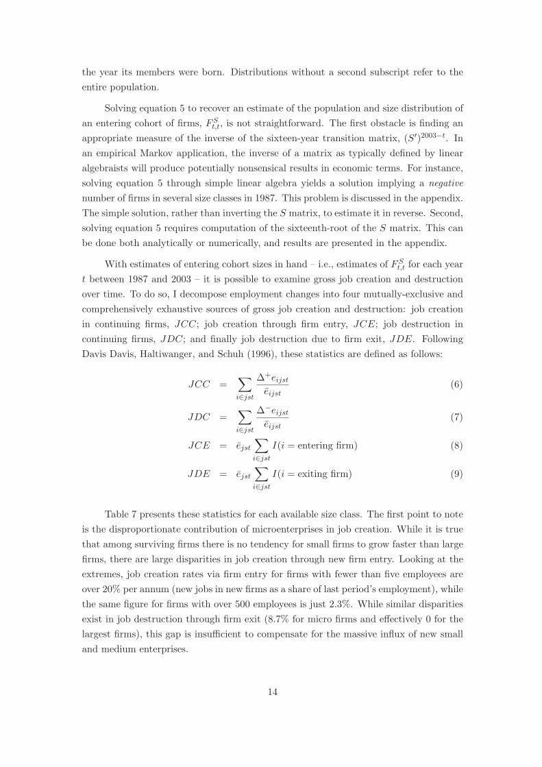
With estimates of entering cohort sizes in hand – i.e., estimates of FSt,t for each year

t between 1987 and 2003 – it is possible to examine gross job creation and destructionover time. To do so, I decompose employment changes into four mutually-exclusive andcomprehensively exhaustive sources of gross job creation and destruction: job creationin continuing firms, JCC; job creation through firm entry, JCE; job destruction incontinuing firms, JDC; and finally job destruction due to firm exit, JDE. FollowingDavis Davis, Haltiwanger, and Schuh (1996), these statistics are defined as follows:

JCC =∑i∈jst

Δ+eijst

eijst(6)

JDC =∑i∈jst

Δ−eijst

eijst(7)

JCE = ejst

∑i∈jst

I(i = entering firm) (8)

JDE = ejst

∑i∈jst

I(i = exiting firm) (9)

Table 7 presents these statistics for each available size class. The first point to noteis the disproportionate contribution of microenterprises in job creation. While it is truethat among surviving firms there is no tendency for small firms to grow faster than largefirms, there are large disparities in job creation through new firm entry. Looking at theextremes, job creation rates via firm entry for firms with fewer than five employees areover 20% per annum (new jobs in new firms as a share of last period’s employment), whilethe same figure for firms with over 500 employees is just 2.3%. While similar disparitiesexist in job destruction through firm exit (8.7% for micro firms and effectively 0 for thelargest firms), this gap is insufficient to compensate for the massive influx of new smalland medium enterprises.

14

Table 8 attempts to put these figures in international perspective. Recent work byBartelsman, Haltiwanger and Scarpetta Bartelsman, Haltiwanger, and Scarpetta (2005)and Haltiwanger, Scarpetta and Schweiger Haltiwanger, Scarpetta, and Schweiger (2006)presents comparable data on the firm size distribution, job creation and job destructionin a range of developing and transition countries. However, these papers present no datafor African or other low income countries, thus Ghana makes an interesting compara-tive case study. As seen in the table, while there is no strong tendency for the share offirms or employment in the small-firm sector to vary with per capita GDP, Ghana firstin both these categories. Ghana is the only country on the list with less than half itsmanufacturing workforce in the large firm sector, defined as greater than 50 employees.However, in terms of both gross and net job reallocation rates by size class, the interna-tional field shows enormous variance, placing Ghana within a fairly standard range. Thisincludes conforming to a slight tendency for the poorer countries in the list to exhibitfaster growth rates in the small and medium enterprise sector during the 1990s relativeto the large firm sector.

5. Underlying Determinants of Growth: The Role of Credit Constraints

Why then do the increasingly large, entering cohorts of micro-enterprises docu-mented above fail to move up through the firm size distribution? As noted in Section2, Table 3, the overwhelming response given by owners and managers of small firms isa lack of access to credit. This is listed as a major obstacle to firm growth by just over69% of both micro- and small-enterprise owners.

This section attempts to take these concerns seriously, presenting a simple modelof the evolution of the firm size distribution in the presence of credit constraints, anddrawing on the GMES data to estimate the quantitative significance of this constraintin explaining the observed distribution dynamics.

I begin with the production side of a neoclassical model of firm size (Lucas, 1978).Eachindividual in the economy is assumed to have some level of managerial talent, θ, whichwill determine the efficiency of any firm he or she manages, and in turn its optimal size.Production is given by

yit = θh[f(nit, kit)] (10)

where f(.) is a standard production function employing capital and labor, couched withina managerial technology, h(.), which is assumed to be concave. Profit maximization basedon (10) yields a solution for optimal firm size measured in employment terms:

n∗ijt(θij) = argmax{θijh[f(nijt, kijt)] − wnijt − rkijt}. (11)

The concavity of the h(.) function ensures that the optimal “span of control” for a

15

manager with a given talent level is well defined even with an underlying constant-returnsto scale production function.

In the language of the growth literature, I focus on transition dynamics. For thesake of empirical analysis, I allow that each firm will have an idiosyncratic long-runequilibrium growth rate, gij , whose determinants are outside the scope of the analysisand will be captured in firm fixed effects.

I introduce credit constraints as an indicator variable, Cij, denoting the inability toacquire finance at the market interest rate. Credit constraints, as I use the term, implya market failure. In contrast, firms which are simply priced out of the market for financeby their inability to pay competitive interest rates would not be considered constrained.

Suppose that each entrepreneur is endowed with initial wealth ω, which for sim-plicity is measured in firm size units (i.e. the maximum number of employees the en-trepreneur can afford to hire). This yields a starting firm size of n∗

ijt if unconstrained andn(ωij) if constrained – i.e., the largest size permitted by the initial capital endowment.

In the subsequent period, unconstrained firms will be on their equilibrium growthpath, gij . Firms facing credit constraints, however, will begin the period at an initialsize dictated by their wealth endowment, and will be able to grow only insomuch as thebusiness generates profits to finance expansion toward the optimal size n∗

ij . Thus firmgrowth will be a function of credit constraints, past profits, and underlying efficiency

Δnijt = Δn(Cij(θij), πijt, θij) (12)

or more explicitly,

Δnijt =

⎧⎪⎨⎪⎩

gij if Cij = 0

min(n∗ijt(θij) − nij,t−1, πij,t−1) if Cij = 1

(13)

The equations in (13) state that unconstrained firms grow at an exogenous rate, whileconstrained growth will be the lesser of the gap between current and optimal size, or theexpansion feasible with available financing.

The model presents a clear empirical test for the presence of credit constraints: prof-its should impact growth only for firms which are suspected to be credit constrained.14

To take the model to the data, as a measure of internal finance I use the log of firm

14This result is closely analogous to a central result from the literature on finance and corporate invest-ment. Based on q-theory, investment by publicly traded firms should be independent of internal liquidityafter controlling for the stock market value of the firm. The significance of internal liquidity measures ininvestment equations has been widely interpreted as an indication of capital market inefficiencies (Fazzari,Hubbard, and Petersen, 1988).

16

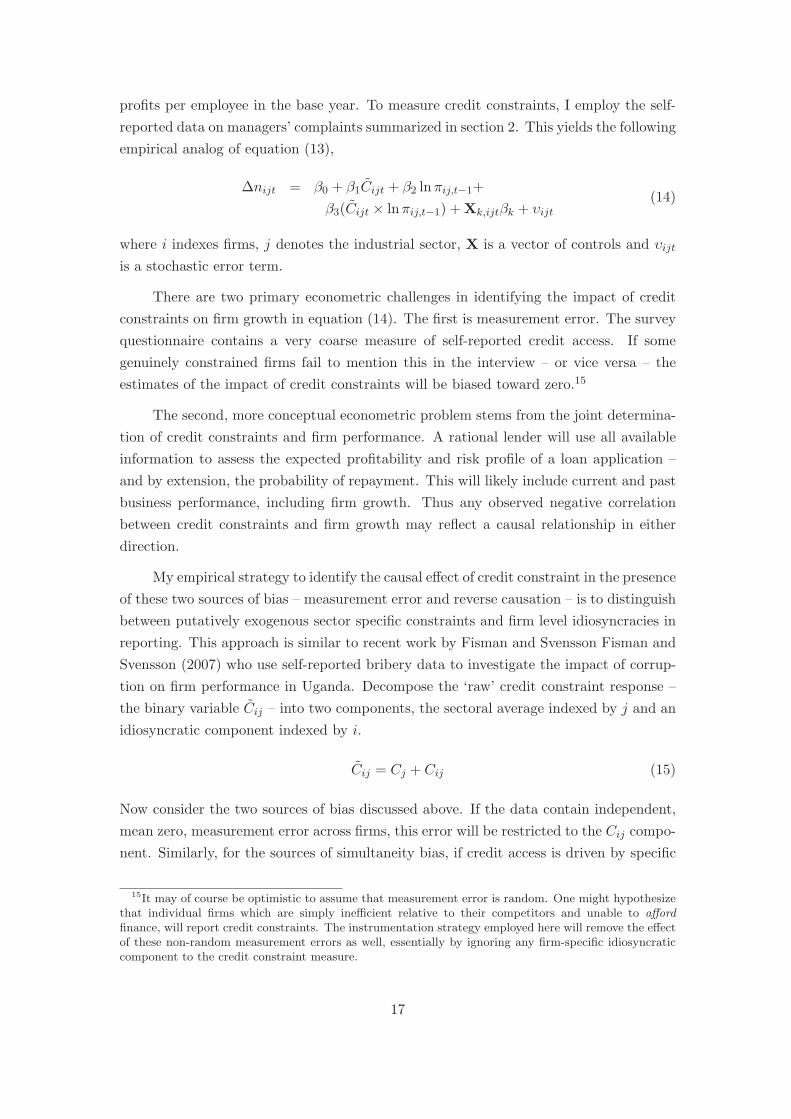
profits per employee in the base year. To measure credit constraints, I employ the self-reported data on managers’ complaints summarized in section 2. This yields the followingempirical analog of equation (13),

Δnijt = β0 + β1Cijt + β2 lnπij,t−1+β3(Cijt × lnπij,t−1) + Xk,ijtβk + υijt

(14)

where i indexes firms, j denotes the industrial sector, X is a vector of controls and υijt

is a stochastic error term.

There are two primary econometric challenges in identifying the impact of creditconstraints on firm growth in equation (14). The first is measurement error. The surveyquestionnaire contains a very coarse measure of self-reported credit access. If somegenuinely constrained firms fail to mention this in the interview – or vice versa – theestimates of the impact of credit constraints will be biased toward zero.15

The second, more conceptual econometric problem stems from the joint determina-tion of credit constraints and firm performance. A rational lender will use all availableinformation to assess the expected profitability and risk profile of a loan application –and by extension, the probability of repayment. This will likely include current and pastbusiness performance, including firm growth. Thus any observed negative correlationbetween credit constraints and firm growth may reflect a causal relationship in eitherdirection.

My empirical strategy to identify the causal effect of credit constraint in the presenceof these two sources of bias – measurement error and reverse causation – is to distinguishbetween putatively exogenous sector specific constraints and firm level idiosyncracies inreporting. This approach is similar to recent work by Fisman and Svensson Fisman andSvensson (2007) who use self-reported bribery data to investigate the impact of corrup-tion on firm performance in Uganda. Decompose the ‘raw’ credit constraint response –the binary variable Cij – into two components, the sectoral average indexed by j and anidiosyncratic component indexed by i.

Cij = Cj + Cij (15)

Now consider the two sources of bias discussed above. If the data contain independent,mean zero, measurement error across firms, this error will be restricted to the Cij compo-nent. Similarly, for the sources of simultaneity bias, if credit access is driven by specific

15It may of course be optimistic to assume that measurement error is random. One might hypothesizethat individual firms which are simply inefficient relative to their competitors and unable to affordfinance, will report credit constraints. The instrumentation strategy employed here will remove the effectof these non-random measurement errors as well, essentially by ignoring any firm-specific idiosyncraticcomponent to the credit constraint measure.

17

knowledge of an individual firm’s efficiency or growth potential, this will again be cap-tured in the Cij term. In contrast, exogenous sources of credit constraints are likely tobe constant across firms in a similar sector, size class or region. For instance, if creditis rationed because of legal difficulties in enforcing repayment in the informal sector, orbecause the fixed costs of lending cannot be justified by the small loans demanded bysmall firms, these effects will be common across firms in the same sector-size-region cell.

In short, endogenous variation is largely captured in the idiosyncratic firm-levelvariation in Cij , while differences across j cells are putatively exogenous. This suggeststhat local means of the credit constraint variable will serve as a valid instrument forfirms’ own reports in equation 14.

A similar problem – and a similar solution – arise in the measurement of profitsas well. Cross-sectional and time-series variation in profits may arise for any number ofreasons, many of which can be treated as exogenous for the purposes of an employmentgrowth regression. For instance, transitory fluctuations in demand, relative prices, inputavailability or costs will constitute a shock to profits which should not affect the firm’soptimal scale. Other sources of variation in profits are more problematic. Variations inmarket power between firms, growth in technical efficiency for a given firm relative toits competitors, and so on should produce effects on firm growth independent of creditconstraints. Measurement error in firms’ profits accounts is of course also a concern.

Once again, I rely on sector averages to instrument firm level profits in equation(14). Decomposing profits in a similar fashion to line (15), the sector specific componentof profits, πj , captures forces that are arguably exogenous to the firm. It is possible toconceive of scenarios which will invalidate this instrument – for instance, a permanenttechnological shock raising the productivity and optimal scale of all firms in a givensector. It should be noted, however, that there is no reason to expect such a shockto have a disproportionately positive effect on credit constrained firms. Thus findinga positive coefficient on β3 remains a putatively valid test for the importance of creditconstraints.

Estimates of equation 14 show strong support for the model in the previous section.Table 9 presents various specifications of this basic model using the GMES data. TheOLS point estimates in column 1 conform to the basic predictions of the model, althoughthe results are insignificant. The insignificant association between the credit constraintsindicator and firm growth is perhaps surprising, but fits with the story of endogeneityabove. If managers who are particularly eager to expand their firms are those whichcomplain of credit constraints, this may mask the true negative impact of the marketfailure. Additionally, simple noise in this self-reported measure of constraints will alsobias the point estimate toward zero and insignificance.

The left side of Table 9 presents instrumental variables estimates of the growth

18

equation, using as instruments the average values of the credit constraint variable withina firm’s sector, size class and region. As with the OLS, the IV point estimates in column3 conform to the basic predictions of the model. In this case, however, the magnitude ofthe effects is dramatically increased and significantly different from zero. On their own,log profits still have effectively zero correlation with firm growth. The instrumentedcredit constraints variable now shows an even larger negative correlation with growth(coefficient of -1.24) and the interaction between credit constraints and log profits issignificant and positive. Adding firm fixed effects to the model in column 4 preventsthe estimation of the simple credit constraints effect, as this variable does not changeover time, but confirms the pattern of interactions with log profits. This pattern ofcoefficients is consistent with a model in which firms gradually overcome lack of creditaccess by financing expansion through internal profits.

Finally, it is worth considering how far these these estimated effects can explain thecollapse of average firm size and the long run tendency toward a right-skewed firm sizedistribution identified in section 4. The predicted values from the regressions give someindication that the actual economic importance of these effects may be quite modest.The average predicted values from the growth model in column 3 for firm with fewerthan 10 and greater than 100 employees are approximately -3.7% and 1.9%, respectively.I simulate the relaxation of credit constraints by re-calculating predicted growth rates,setting the credit constraint variable (and its interaction with profits) to zero for allfirms. The predicted rate for small firms rises from -3.7% to -2.1%, while that for largefirms is virtually unchanged at 1.9% and 1.5% with and without constraints, reflectingthe near absence of credit constraints in this size class. What is noteworthy is that, whilethe gap between small and large firms for these ‘unconstrained’ growth rates is reduced,the difference is not dramatic. Importantly, they suggest that even a major interventionto overcome credit market failures would be insufficient to produce convergence betweenlarge and small firms or correct the right skewness in the ergodic firm size distribution.

6. Conclusions

In 1994 the World Bank published a widely cited review of reform efforts in Africa(World Bank, 1994), written partly as a response to critics who argued that Bank-fundedstructural adjustment programs had entailed social displacement and industrial decline(Stewart, Lall, and Wangwe, 1992). In the discussion of industrial development, thereport drew on the first three rounds of the RPED surveys in Ghana to defend the trackrecord of liberalization.

The picture in Ghana, the country with the most extensive adjustment, isnot one of stagnation and deindustrialization; instead, it shows much activ-ity, particularly among smaller enterprises not included in official statistics.(World Bank, 1994, p. 149)

19

In short, the early RPED studies were already pointing to the boom in microenterpriseactivity. The report acknowledged, however, that there was not – circa 1994 – sufficientevidence to fully investigate the impact of liberalization on industrial development or jobcreation.

The big question is whether the activity of small firms is a structuralbreak with the past or simply a sign of distress. Are many of the smallernew entrants simply household efforts to survive at the margin, or are theydynamic new enterprises that can significantly increase employment in thefuture? (World Bank, 1994, p. 152)

More than a decade later, data now exist to answer this question. Two cleardepartures from existing ‘stylized facts’ in the literature emerged from the analysis offirm entry, growth and exit between 1987 and 2003. First, contrary to previous studieson African data sets which have ignored firm entry (and a wealth of evidence on U.S.data), I find that microenterprises accounted for the bulk of gross and net job creationover the period from 1987 to 2003. Massive new entry of small firms drove average firmsize in the sector down by over 50%. Second, contrary to findings from developed countrydata sets, these entering firms do not appear destined to become medium or large scaleenterprises over time. It is selection, rather than within-firm growth, that drives theapparent ‘life-cycle of firms’ observed in cross-sectional data.

The contrast with results from developed country data sets on this front is extremelytelling. Were the same explosion of entrepreneurial activity taking place in Portugal,there would be reason to believe that the influx of new firms contained the seeds offuture large scale industrial development. Such is not the case in Ghana. Existingevidence suggests that small enterprises die early and small. Conversely, big firms don’trepresent successful microentrepreneurs that have risen through the ranks of smallerfirms. Rather, big firms are born big.

The final part of the paper examined the potential for improvements in the function-ing of credit-markets to promote growth among small and microenterprises. Instrumentalvariables estimates provide compelling evidence that credit constraints constitute a sig-nificant drag on firm growth. Rather than dissipating over time, these constraints havea permanent effect on the firm size distribution and may contribute to significant ineffi-ciencies in resource allocation. However, the importance of credit constraints should notbe oversold. My econometric evidence suggests that removing such constraints would beinsufficient to overcome the downward slide in the firm size distribution. Further analysisof the role of credit constraints at the point of firm entry may shed additional light onthis topic.

From a policy perspective, the Ghanaian experience calls into question the assumedlink between market reforms and the decline of the informal sector, or the emergence ofa robust large-firm sector. Additionally, policy prescriptions stressing credit market in-terventions to overcome slow-growth among microenterprises require further justification

20

as credit constraints cannot fully account for the right skewness in the Ghanaian data.From a methodological perspective, the main lesson of this paper is the need to accountexplicitly for firm entry in the analysis of industrial dynamics. In the design of futuredata collection efforts, one simple improvement would be to rely on rolling panels thataccount for changes in the broader distribution of firms, rather than relying exclusivelyon cross-sections or tracking a fixed sample of firms, as in most existing panel data setsfrom low-income countries.

Appendix: Further Details on the Calculation of Entry Rates

A. Reversing the Markov Chain

To calculate the distribution of entering firm cohorts it is necessary to solve equation5 to recover an estimate of FS

t,t. Simplifying notation for illustrative purposes, I rewritethis equation as

Ft = StF0

so that the goal is to recover F0. Solving for F0 is complicated by the fact that St isestimated with error. Due to this measurement error, it is clear that

F0 = S−tFt and

= S−tFt, but

�= S−tFt, (16)

where hats denote empirical estimates, S−t is the matrix inverse of St, and St is inturn the tth power of the S matrix. Even if the transition matrix is estimated withreasonable precision, St ≈ St, the expression in line (16) may fail to provide even arough approximation to the F0 distribution. This is because the process of inverting anestimated matrix will magnify the effect of measurement error exponentially.

The solution is to estimate the transition matrix in reverse, which I label Str. This

‘reverse matrix’ is based on a multinomial logit model, identical to equation 2, but withthe dependent and independent variables transposed – i.e., starting size classes are afunction of ending size classes. Thus element mn of the St

r matrix gives the probabilityof beginning in size class m conditional on ending up in size class n. Using this calculationI can empirically confirm that F0 ≈ St

rFt. Estimates of Str based on the NIC data for

the sixteen year span from 2003 to 1987 are presented in the top panel of Table 10.

Mathematically, these two distinct matrices – the algebraic inverse and the ‘reversetransition matrix’ – represent just two of the infinite possible solutions to the system ofequations embodied in 5. Crucially, the reverse matrix is the solution suggested by thedata.

21

B. Using the Markov Chain to Estimate Entering Cohorts

Using the estimates of the sixteen-year reverse transition matrix, it is possible torecreate the implied initial distribution of firms at time zero (in this case, 1987) basedon the distribution in time t (2003). While this is empirically uninteresting – as the 1987distribution is directly observed – it is possible to use the same method to recreate thedistribution of firms at other points in time that are not directly observable.

In particular, I am interested in estimating the distribution of entering cohorts –the distribution of firm size in, say, 2002 of firms born in that same period. To doso, I begin with the distribution of firms born in 2002 which survived until 2003. Thedistribution of these survivors has clearly evolved since entry, both through exit and sizeclass transitions. To recreate their initial distribution, I multiply the ending distributionby the one-year reverse transition matrix and the inverse of the death matrix, as impliedby equation 5. To estimate entering cohorts in a give year, t, by this method requires anestimate of the transition probabilities over the time period 2003 − t. These transitionprobabilities can be calculated as the roots and powers of the St

r matrix.

C. Calculating Roots and Powers of the Markov Chain

Define the square-root of a matrix S, such that S = S1/2S1/2. If S is a diagonalmatrix, its square root can be formed by taking the square root of each of its individualdiagonal entries. The same procedure holds for any square matrix that is diagonalizable.

The q×q matrix S is diagonalizable if there is a matrix V such that D = V −1SV isa diagonal matrix. If S has q independent eigenvectors, V can be formed by the matrixwhose columns are these q eigenvectors. Diagonalization presents an efficient method forcalculating the powers, or roots, of a matrix, as

S1/2 = V −1D1/2V

and so on for other powers of S.

In empirical applications, an alternative method to this diagonalization is to relyon a numerical approximation. Let Y0 = S and Z0 = I(q), the q × q identity matrix.Denman and Beavers Denman and Beavers (1976) show that through iteration of thefollowing algorithm,

Yk+1 = 12(Yk + Z−1

k ), (17)

Zk+1 = 12(Y −1

k + Zk) (18)

Yk converges quadratically to the square root of S.

22

The bottom panel of Table 10 reports the sixteenth-root of the reverse transitionmatrix in the top panel, based on the Denman-Beavers algorithm. As a check, I alsocalculated the same matrix by diagonalization using a mathematical software package(Maple) and reached an indistinguishable result. The estimates in Table 10 are used asthe basis to calculate entering cohorts in section 4 of the main text.

References

Appiah-Kubi, K. (2001): “State-Owned Enterprises and Privatisation in Ghana,” Jour-nal of Modern African Studies, 39(2), 197–229.

Aryeetey, E., and A. McKay (2007): “Ghana: The Challenge of Translating Sus-tained Growth into Poverty Reduction,” in Delivering on the Promise of Pro-PoorGrowth: Insights and Lessons from Country Experiences, ed. by L. Cord. New York:Palgrave Macmillan.

Asante, Y., F. Nixson, and K. Tsikata (2000): “The Industrial Sector Policies &Economic Development,” in Economic Reform in Ghana: The Miracle and the Mirage,ed. by E. Aryeetey, and J. Harrigan. Oxford: James Currey, Ltd.

Bartelsman, E., J. Haltiwanger, and S. Scarpetta (2005): “Measuring and An-alyzing Cross-Country Differences in Firm Dynamics,” National Bureau of EconomicResearch.

Beck, T., A. Demirguc-Kunt, and R. Levine (2003): “Small and Medium Enter-prises, Growth, and Poverty: Cross-Country Evidence,” World Bank Policy ResearchWorking Paper No. 3178.

Besley, T., and R. Burgess (2004): “Can Labor Regulation Hinder Economic Per-formance? Evidence from India,” Quarterly Journal of Economics, 119(1), 91–134.

Bigsten, A., P. Collier, S. Dercon, M. Fafchamps, B. Gauthier, J. Gunning,

A. Isaksson, A. Oduro, R. Oostendorp, C. Pattillo, M. Soderbom, F. Teal,

and A. Zeufack (2003): “Credit Constraints in Manufacturing Enterprises in Africa,”Journal of African Economies, 12(1), 104–25.

Botero, J. C., S. Djankov, R. La Porta, F. Lopez de Silanes, and A. Shleifer

(2004): “The Regulation of Labor,” Quarterly Journal of Economics, 119(4), 1339–82.

Cabral, L. M. B., and J. Mata (2003): “On the Evolution of the Firm Size Distri-bution: Facts and Theory,” American Economic Review, 93(4), 1075–90.

Davis, S., J. Haltiwanger, and S. Schuh (1996): Job Creation and Destruction.MIT Press, Boston.

23

de Soto, H. (1989): The Other Path. New York: Harper and Row.

Denman, E., and A. Beavers (1976): “The matrix sign function and computations insystems,” Applied Mathematics and Computation, 2, 63–94.

Fafchamps, M. (2000): “Ethnicity and Credit in African Manufacturing,” Journal ofDevelopment Economics, 61, 205–35.

Fazzari, S. M., R. G. Hubbard, and B. C. Petersen (1988): “Financing Con-straints and Corporate Investment,” Brookings Papers on Economic Activity, 0(1),141–95.

Fisman, R., and J. Svensson (2007): “Are corruption and taxation really harmful togrowth? Firm level evidence,” Journal of Development Economics, 83, 63 – 75.

Frazer, G. (2005): “Which Firms Die? A Look at Manufacturing Firm Exit in Ghana,”Economic Development and Cultural Change.

Ghana Statistical Service (1984): “Report on the 1984 Population and HousingCensus,” Statistical Service, P.O. Box 1098, Accra, Ghana.

(1989a): “Ghana Directory of Industrial Establishments, 1988,” StatisticalService, P.O. Box 1098, Accra, Ghana.

(1989b): “Ghana National Industrial Census, 1987: Phase 1 Report, Back-ground and Results,” Statistical Service, P.O. Box 1098, Accra, Ghana.

(2000): “Demographic, Health and Economic Characteristics: Report on the2000 Population and Housing Census,” Statistical Service, P.O. Box 1098, Accra,Ghana.

Grayson, L. (1973): “A Conglomerate in Africa: Public-Sector Manufacturing Enter-prises in Ghana, 1962-1971,” African Studies Review, 16(3), 315–345.

Haltiwanger, J., S. Scarpetta, and H. Schweiger (2006): “Assessing Job Flowsacross Countries: The Role of Industry, Firm Size, and Regulations,” World BankPolicy Research Working Paper No. 4070.

Herbst, J. (1993): The Politics of Reform in Ghana, 1982-1991. University of CaliforniaPress, Berkeley and Los Angeles.

Hopenhayn, H. A. (1992): “Entry, Exit, and Firm Dynamics in Long Run Equilib-rium,” Econometrica, 60(5), 1127–50.

Jebuni, C. D., A. D. Oduro, and K. A. Tutu (1994): “Trade and Payments Regimeand the Balance of Payments in Ghana,” World Development, 22(8).

24

Jovanovic, B. (1982): “Selection and the Evolution of Industry,” Econometrica, 50(3),649–70.

Killick, T. (1978): Development Economics in Action: A Study of Economic Policiesin Ghana. Heinemann, London.

Kingdon, G., J. Sandefur, and F. Teal (2006): “Labour Market Flexibility, Wagesand Incomes in Sub-Saharan Africa in the 1990s,” African Development Review, 18(3).

Kumar, K., R. Rajan, and L. Zingales (1999): “What Determines Firm Size?,”Centre for Economic Policy Research (CEPR) Discussion Paper No. 2211.

Lall, S. (1995): “Structural Adjustment and African Industry,” World Development,23(12), 2019–2031.

Lucas, R. E. (1978): “On the Size Distribution of Business Firms,” Bell Journal ofEconomics, 9(2), 508–23.

Quah, D. T. (1997): “Empirics for Growth and Distribution: Stratification, Polariza-tion, and Convergence Clubs,” Journal of Economic Growth, 2(1), 27–59.

Rauch, J. E. (1991): “Modelling the Informal Sector Formally,” Journal of DevelopmentEconomics, 35(1), 33–47.

Shiferaw, A., and A. S. Bedi (2009): “The Dynamics of Job Creation and JobDestruction: Is Sub-Saharan Africa Different?,” IZA Discussion Papers 4623, Institutefor the Study of Labor (IZA).

Soderbom, M., and F. Teal (2004): “Size and Efficiency in African ManufacturingFirms: Evidence from Firm-Level Panel Data,” Journal of Development Economics,73(1), 369–94.

Soderbom, M., F. Teal, and A. Wambugu (2005): “Unobserved Heterogeneity andthe Relation between Earnings and Firm Size: Evidence from Two Developing Coun-tries,” Economics Letters, 87(2), 153–59.

Stewart, F., S. Lall, and S. Wangwe (1992): “Structural Problems of AfricanIndustry,” in Alternative Development Strategies in Sub-Saharan Africa. Macmillan,London.

Sutton, J. (1997): “Gibrat’s Legacy,” Journal of Economic Literature, 35(1), 40–59.

Teal, F. (1999): “The Ghanaian Manufacturing Sector 1991-95: Firm Growth, Pro-ductivity and Convergence,” Journal of Development Studies, 36(1), 109–127.

Tignor, R. L. (2006): W. Arthur Lewis and the Birth of Development Economics.Princeton University Press, Princeton, NJ.

25

Van Biesebroeck, J. (2005): “Firm Size Matters: Growth and Productivity Growth inAfrican Manufacturing,” Economic Development and Cultural Change, 53(3), 545–83.

World Bank (1994): Adjustment in Africa: Reforms, Results, and the Road Ahead.Oxford University Press, New York, NY.

26

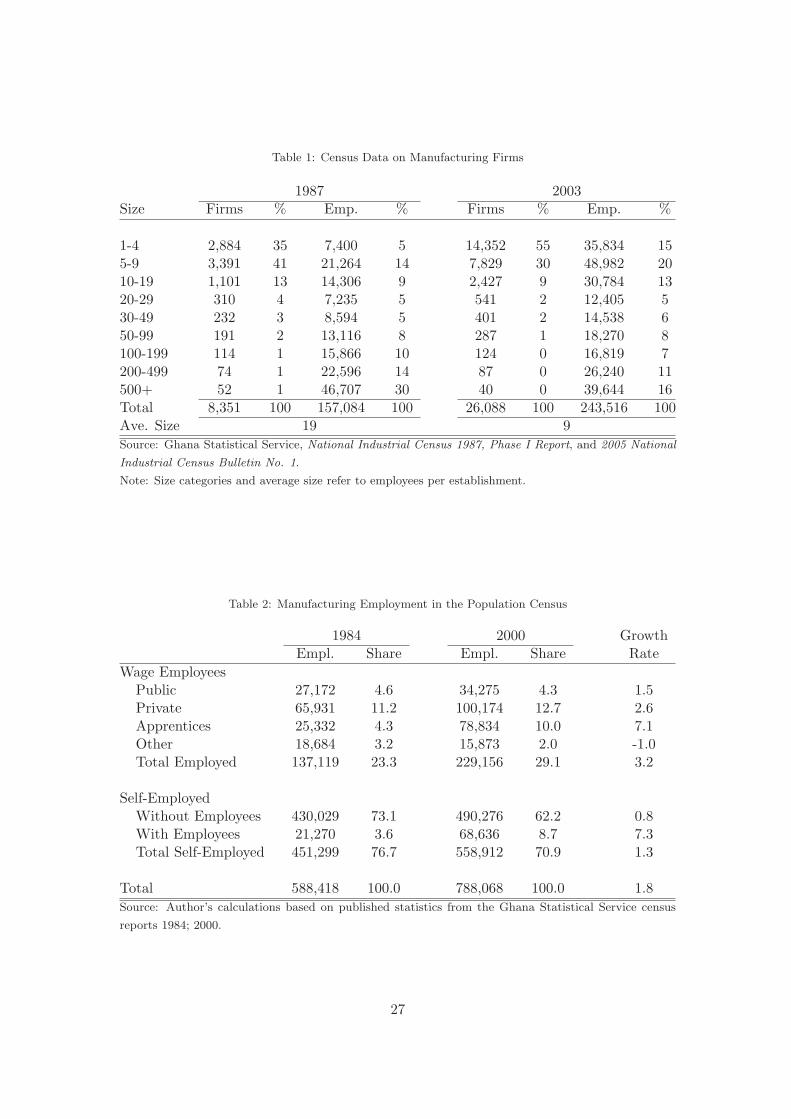
Table 1: Census Data on Manufacturing Firms

1987 2003Size Firms % Emp. % Firms % Emp. %

1-4 2,884 35 7,400 5 14,352 55 35,834 155-9 3,391 41 21,264 14 7,829 30 48,982 2010-19 1,101 13 14,306 9 2,427 9 30,784 1320-29 310 4 7,235 5 541 2 12,405 530-49 232 3 8,594 5 401 2 14,538 650-99 191 2 13,116 8 287 1 18,270 8100-199 114 1 15,866 10 124 0 16,819 7200-499 74 1 22,596 14 87 0 26,240 11500+ 52 1 46,707 30 40 0 39,644 16Total 8,351 100 157,084 100 26,088 100 243,516 100Ave. Size 19 9Source: Ghana Statistical Service, National Industrial Census 1987, Phase I Report, and 2005 National

Industrial Census Bulletin No. 1.

Note: Size categories and average size refer to employees per establishment.

Table 2: Manufacturing Employment in the Population Census

1984 2000 GrowthEmpl. Share Empl. Share Rate

Wage EmployeesPublic 27,172 4.6 34,275 4.3 1.5Private 65,931 11.2 100,174 12.7 2.6Apprentices 25,332 4.3 78,834 10.0 7.1Other 18,684 3.2 15,873 2.0 -1.0Total Employed 137,119 23.3 229,156 29.1 3.2

Self-EmployedWithout Employees 430,029 73.1 490,276 62.2 0.8With Employees 21,270 3.6 68,636 8.7 7.3Total Self-Employed 451,299 76.7 558,912 70.9 1.3

Total 588,418 100.0 788,068 100.0 1.8Source: Author’s calculations based on published statistics from the Ghana Statistical Service census

reports 1984; 2000.

27

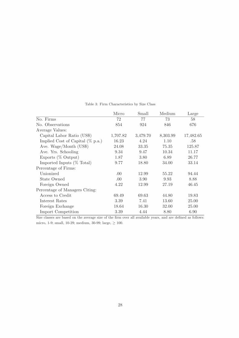
Table 3: Firm Characteristics by Size Class

Micro Small Medium LargeNo. Firms 72 77 73 58No. Observations 854 924 846 676Average Values:

Capital Labor Ratio (US$) 1,707.82 3,479.70 8,303.99 17,482.65Implied Cost of Capital (% p.a.) 16.23 4.24 1.10 .58Ave. Wage/Month (US$) 24.08 33.35 75.35 125.87Ave. Yrs. Schooling 9.34 9.47 10.34 11.17Exports (% Output) 1.87 3.80 6.89 26.77Imported Inputs (% Total) 9.77 18.80 34.00 33.14

Percentage of Firms:Unionized .00 12.99 55.22 94.44State Owned .00 3.90 9.93 8.88Foreign Owned 4.22 12.99 27.19 46.45

Percentage of Managers Citing:Access to Credit 69.49 69.63 44.80 19.83Interest Rates 3.39 7.41 13.60 25.00Foreign Exchange 18.64 16.30 32.00 25.00Import Competition 3.39 4.44 8.80 6.90

Size classes are based on the average size of the firm over all available years, and are defined as follows:

micro, 1-9; small, 10-29; medium, 30-99; large, ≥ 100.

28

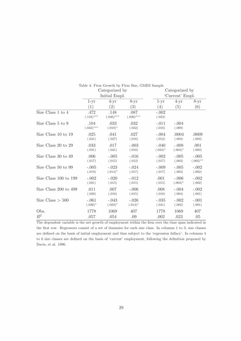
Table 4: Firm Growth by Firm Size, GMES Sample

Categorized by Categorized byInitial Empl. ‘Current’ Empl.

1-yr 4-yr 8-yr 1-yr 4-yr 8-yr(1) (2) (3) (4) (5) (6)

Size Class 1 to 4 .472 .148 .087 -.002(.133)∗∗∗ (.046)∗∗∗ (.030)∗∗∗ (.023)

Size Class 5 to 9 .104 .033 .032 -.011 -.004(.032)∗∗∗ (.018)∗ (.022) (.016) (.009)

Size Class 10 to 19 .025 .041 .027 -.004 .0004 .0009(.021) (.027) (.018) (.012) (.004) (.004)

Size Class 20 to 29 .033 .017 -.003 -.040 -.008 .001(.031) (.021) (.010) (.024)∗ (.004)∗ (.003)

Size Class 30 to 49 .006 -.005 -.016 -.002 -.005 -.005(.017) (.015) (.012) (.017) (.003) (.002)∗∗

Size Class 50 to 99 -.005 -.023 -.024 -.009 -.005 -.002(.019) (.014)∗ (.017) (.017) (.003) (.002)

Size Class 100 to 199 -.002 -.020 -.012 .001 -.006 -.002(.021) (.015) (.015) (.015) (.003)∗ (.002)

Size Class 200 to 499 .011 .007 -.006 .008 -.004 -.002(.020) (.016) (.015) (.018) (.004) (.001)

Size Class > 500 -.061 -.043 -.026 -.035 -.002 -.001(.036)∗ (.023)∗ (.014)∗ (.041) (.002) (.001)

Obs. 1778 1069 407 1778 1069 407R2 .057 .054 .09 .002 .023 .05The dependent variable is the net growth of employment within the firm over the time span indicated in

the first row. Regressors consist of a set of dummies for each size class. In columns 1 to 3, size classes

are defined on the basis of initial employment and thus subject to the ‘regression fallacy’. In columns 4

to 6 size classes are defined on the basis of ‘current’ employment, following the definition proposed by

Davis, et al. 1996.

29

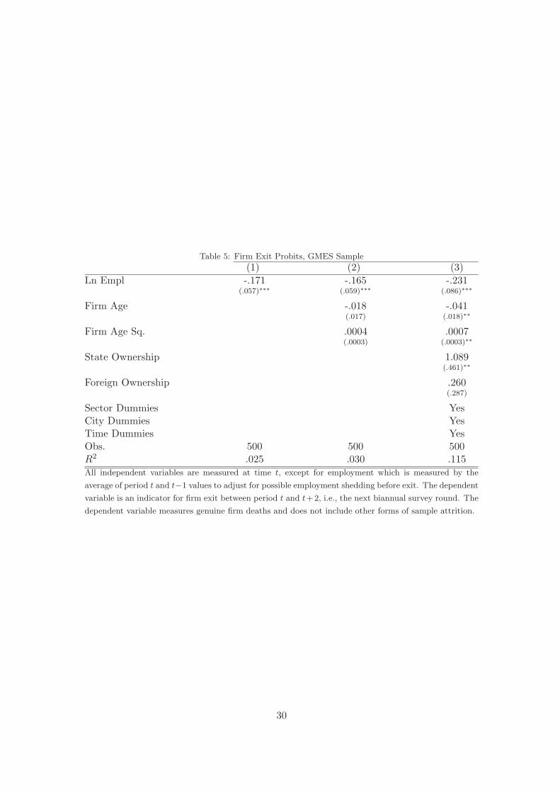
Table 5: Firm Exit Probits, GMES Sample

(1) (2) (3)Ln Empl -.171 -.165 -.231

(.057)∗∗∗ (.059)∗∗∗ (.086)∗∗∗

Firm Age -.018 -.041(.017) (.018)∗∗

Firm Age Sq. .0004 .0007(.0003) (.0003)∗∗

State Ownership 1.089(.461)∗∗

Foreign Ownership .260(.287)

Sector Dummies YesCity Dummies YesTime Dummies YesObs. 500 500 500R2 .025 .030 .115All independent variables are measured at time t, except for employment which is measured by the

average of period t and t−1 values to adjust for possible employment shedding before exit. The dependent

variable is an indicator for firm exit between period t and t+2, i.e., the next biannual survey round. The

dependent variable measures genuine firm deaths and does not include other forms of sample attrition.

30

Table

6:

Mult

inom

ialLogit

Est

imate

softh

e16-Y

ear

Tra

nsi

tion

Matr

ix,N

ICSam

ple

1to

45

to9

10to

1920

to29

30to

4950

to99

100

to19

920

0to

499

500+

1to

4.6

88.3

13(.

067)

(.067)

5to

9.3

55.3

98.1

40.0

86.0

11.0

11(.

050)

(.051)

(.036)

(.029)

(.011)

(.011)

10to

19.1

67.2

96.1

85.1

48.1

30.0

56.0

19(.

051)

(.062)

(.053)

(.048)

(.046)

(.031)

(.018)

20to

29.0

67.1

33.4

00.1

33.2

00.0

67(.

064)

(.088)

(.126)

(.088)

(.103)

(.064)

30to

49.0

50.1

50.1

00.3

50.1

50.1

00.1

00(.

049)

(.080)

(.067)

(.107)

(.080)

(.067)

(.067)

50to

99.1

25.0

83.2

08.4

17.1

25.0

42(.

068)

(.056)

(.083)

(.101)

(.068)

(.041)

100

to19

9.0

40.0

80.1

20.1

20.2

00.0

80.2

80.0

80(.

039)

(.054)

(.065)

(.065)

(.080)

(.054)

(.090)

(.054)

200

to39

9.0

53.2

11.4

74.2

63(.

051)

(.094)

(.115)

(.101)

500

+.5

71.4

29(.

187)

(.187)

Erg

odic

.322

.221

.086

.053

.059

.050

.034

.114

.061

The

left

colu

mn

list

sst

art

ing

size

sand

the

top

row

list

sen

din

gsi

zes.

Entr

ies

inth

eta

ble

repre

sent

row

pro

babilit

ies,

i.e.

,th

epro

bability

that

afirm

start

ing

ina

giv

enro

ww

illen

din

agiv

enco

lum

n.

All

row

ssu

mto

one.

Sta

ndard

erro

rsare

list

edin

pare

nth

eses

.

31

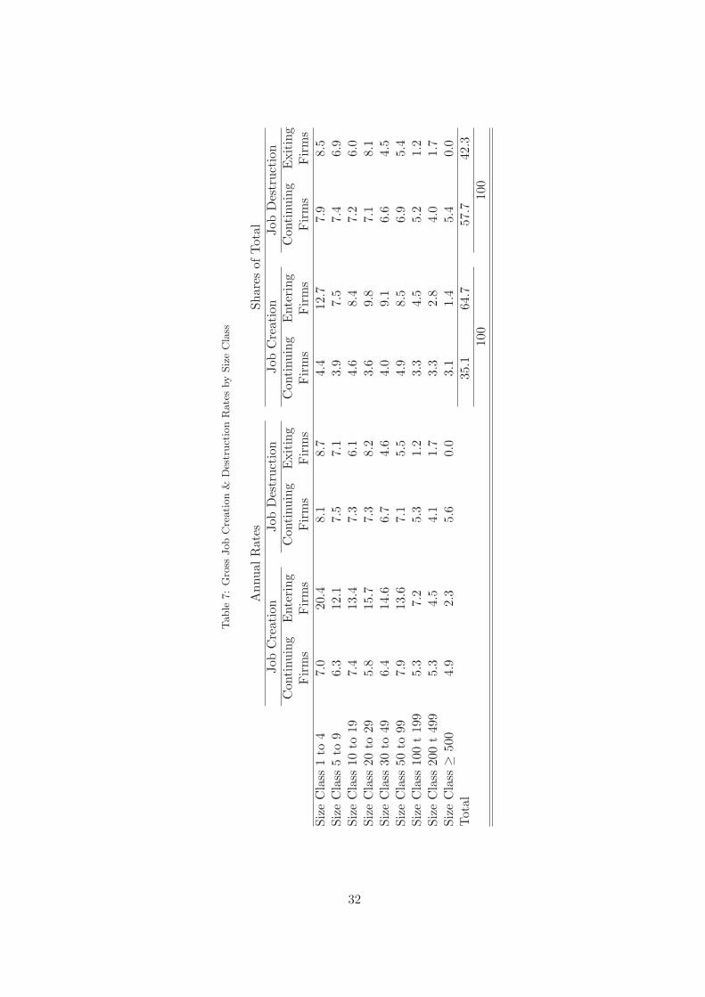
Table

7:

Gro

ssJob

Cre

ati

on

&D

estr

uct

ion

Rate

sby

Siz

eC

lass

Ann

ualR

ates

Shar

esof

Tot

alJo

bC

reat

ion

Job

Des

truc

tion

Job

Cre

atio

nJo

bD

estr

ucti

onC

onti

nuin

gE

nter

ing

Con

tinu

ing

Exi

ting

Con

tinu

ing

Ent

erin

gC

onti

nuin

gE

xiti

ngFir

ms

Fir

ms

Fir

ms

Fir

ms

Fir

ms

Fir

ms

Fir

ms

Fir

ms

Size

Cla

ss1

to4

7.0

20.4

8.1

8.7

4.4

12.7

7.9

8.5

Size

Cla

ss5

to9

6.3

12.1

7.5

7.1

3.9

7.5

7.4

6.9

Size

Cla

ss10

to19

7.4

13.4

7.3

6.1

4.6

8.4

7.2

6.0

Size

Cla

ss20

to29

5.8

15.7

7.3

8.2

3.6

9.8

7.1

8.1

Size

Cla

ss30

to49

6.4

14.6

6.7

4.6

4.0

9.1

6.6

4.5

Size

Cla

ss50

to99

7.9

13.6

7.1

5.5

4.9

8.5

6.9

5.4

Size

Cla

ss10

0t

199

5.3

7.2

5.3

1.2

3.3

4.5

5.2

1.2

Size

Cla

ss20

0t

499

5.3

4.5

4.1

1.7

3.3

2.8

4.0

1.7

Size

Cla

ss≥

500

4.9

2.3

5.6

0.0

3.1

1.4

5.4

0.0

Tot

al35

.164

.757

.742

.310

010

0

32

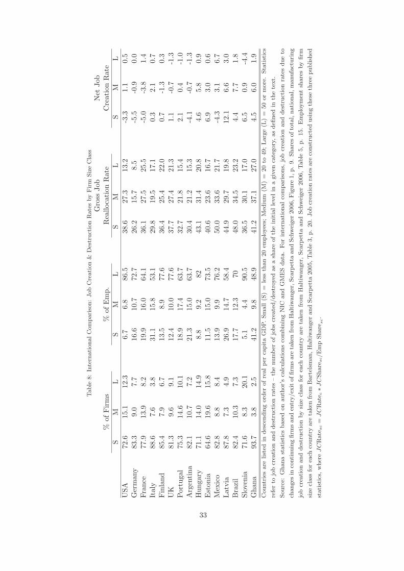
Table

8:

Inte

rnati

onalC

om

pari

son:

Job

Cre

ati

on

&D

estr

uct

ion

Rate

sby

Fir

mSiz

eC

lass

Gro

ssJo

bN

etJo

b%

ofFir

ms

%of

Em

p.R

eallo

cati

onR

ate

Cre

atio

nR

ate

SM

LS

ML

SM

LS

ML

USA

72.6

15.1

12.3

6.7

6.8

86.5

38.6

27.3

13.2

-3.3

1.1

0.5

Ger

man

y83

.39.

07.

716

.610

.772

.726

.215

.78.

5-5

.5-0

.90.

0Fr

ance

77.9

13.9

8.2

19.9

16.0

64.1

36.1

27.5

25.5

-5.0

-3.8

1.4

Ital

y88

.67.

63.

831

.115

.853

.129

.819

.517

.10.

32.

10.

7Fin

land

85.4

7.9

6.7

13.5

8.9

77.6

36.4

25.4

22.0

0.7

-1.3

0.3

UK

81.3

9.6

9.1

12.4

10.0

77.6

37.7

27.4

21.3

1.1

-0.7

-1.3

Por

tuga

l75

.314

.610

.118

.917

.463

.732

.721

.815

.42.

10.

4-1

.0A

rgen

tina

82.1

10.7

7.2

21.3

15.0

63.7

30.4

21.2

15.3

-4.1

-0.7

-1.3

Hun

gary

71.1

14.0

14.9

8.8

9.2

8243

.131

.420

.84.

65.

80.

9E

ston

ia64

.619

.615

.811

.515

.073

.540

.623

.616

.76.

93.

00.

6M

exic

o82

.88.

88.

413

.99.

976

.250

.033

.621

.7-4

.33.

16.

7Lat

via

87.8

7.3

4.9

26.9

14.7

58.4

44.9

29.7

19.8

12.1

6.6

3.0

Bra

zil

82.4

10.3

7.3

17.7

12.3

7048

.034

.523

.24.

47.

71.

8Sl

oven

ia71

.68.

320

.15.

14.

490

.536

.530

.117

.06.

50.

9-4

.4G

hana

93.7

3.8

2.5

41.2

9.8

48.9

41.2

37.1

27.0

4.5

6.0

1.9

Countr

ies

are

list

edin

des

cendin

gord

erof

realper

capit

aG

DP.Sm

all

(S)

=le

ssth

an

20

emplo

yee

s;M

ediu

m(M

)=

20

to49;Larg

e(L

)=

50

or

more

.Sta

tist

ics

refe

rto

job

crea

tion

and

des

truct

ion

rate

s–

the

num

ber

ofjo

bs

crea

ted/des

troy

edas

ash

are

ofth

ein

itia

lle

vel

ina

giv

enca

tegory

,as

defi

ned

inth

ete

xt.

Sourc

e:G

hana

stati

stic

sbase

don

auth

or’

sca

lcula

tions

com

bin

ing

NIC

and

GM

ES

data

.For

inte

rnati

onalco

mpari

sons,

job

crea

tion

and

des

truct

ion

rate

sdue

to

changes

inco

nti

nuin

gfirm

sand

entr

y/ex

itoffirm

sare

taken

from

Halt

iwanger

,Sca

rpet

taand

Sch

wei

ger

2006,Fig

ure

1,p.

9.

Share

softo

tal,

nati

onal,

manufa

cturi

ng

job

crea

tion

and

des

truct

ion

by

size

class

for

each

countr

yare

taken

from

Halt

iwanger

,Sca

rpet

taand

Sch

wei

ger

2006,Table

5,p.

15.

Em

plo

ym

ent

share

sby

firm

size

class

for

each

countr

yare

taken

from

Bart

elsm

an,H

alt

iwanger

and

Sca

rpet

ta2005,Table

3,p.

20.

Job

crea

tion

rate

sare

const

ruct

edusi

ng

thes

eth

ree

publish

ed

stati

stic

s,w

her

eJC

Rate

sc

=JC

Rate

c∗J

CShare

sc/E

mp

Share

sc.

33

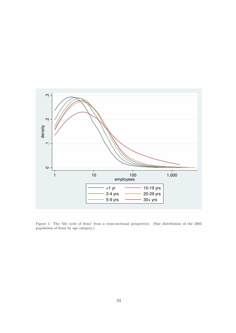
0.1

.2.3

dens

ity

1 10 100 1,000employees

<1 yr 10-19 yrs2-4 yrs 20-29 yrs5-9 yrs 30+ yrs

Figure 1: The ‘life cycle of firms’ from a cross-sectional perspective. (Size distribution of the 2003population of firms by age category.)

34

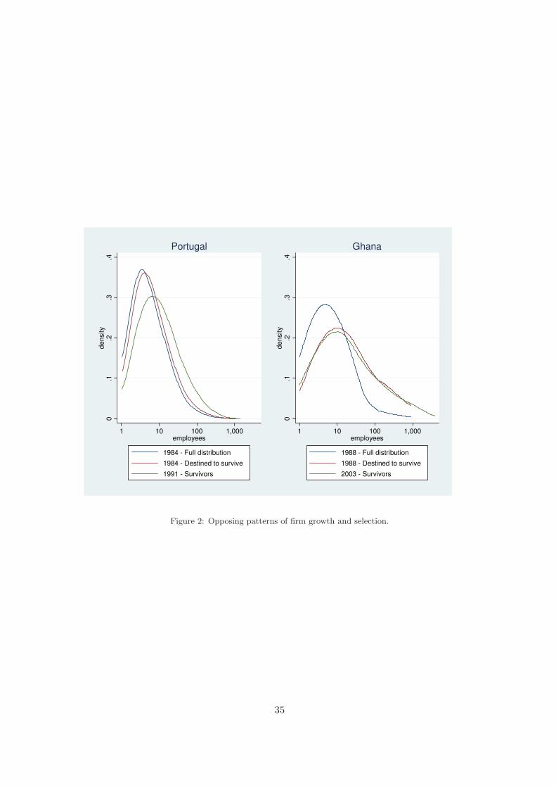
0.1

.2.3

.4de

nsity

1 10 100 1,000employees

1984 - Full distribution

1984 - Destined to survive

1991 - Survivors

Portugal

0.1

.2.3

.4de

nsity

1 10 100 1,000employees

1988 - Full distribution

1988 - Destined to survive

2003 - Survivors

Ghana

Figure 2: Opposing patterns of firm growth and selection.

35

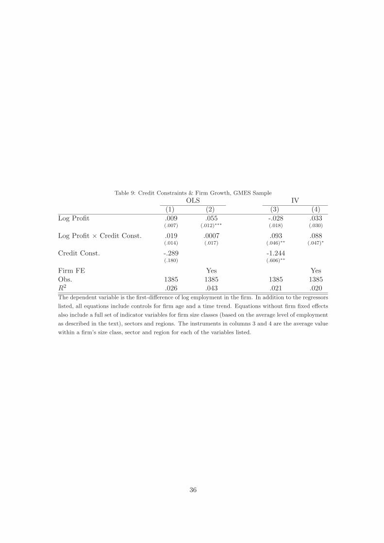
Table 9: Credit Constraints & Firm Growth, GMES Sample

OLS IV(1) (2) (3) (4)

Log Profit .009 .055 -.028 .033(.007) (.012)∗∗∗ (.018) (.030)

Log Profit × Credit Const. .019 .0007 .093 .088(.014) (.017) (.046)∗∗ (.047)∗

Credit Const. -.289 -1.244(.180) (.606)∗∗

Firm FE Yes YesObs. 1385 1385 1385 1385R2 .026 .043 .021 .020The dependent variable is the first-difference of log employment in the firm. In addition to the regressors

listed, all equations include controls for firm age and a time trend. Equations without firm fixed effects

also include a full set of indicator variables for firm size classes (based on the average level of employment

as described in the text), sectors and regions. The instruments in columns 3 and 4 are the average value

within a firm’s size class, sector and region for each of the variables listed.

36

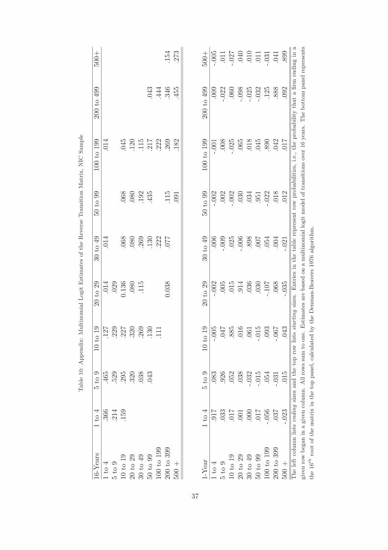
Table

10:

Appen

dix

:M

ult

inom

ialLogit

Est

imate

softh

eR

ever

seTra

nsi

tion

Matr

ix,N

ICSam

ple

16-Y

ears

1to

45

to9

10to

1920

to29

30to

4950

to99

100

to19

920

0to

499

500+

1to

4.3

66.4

65.1

27.0

14.0

14.0

145

to9

.214

.529

.229

.029

10to

19.1

59.2

95.2

270.

136

.068

.068

.045

20to

29.3

20.3

20.0

80.0

80.0

80.1

2030

to49

.038

.269

.115

.269

.192

.115

50to

99.0

43.1

30.1

30.4

35.2

17.0

4310

0to

199

.111

.222

.222

.444

200

to39

90.

038

.077

.115

.269

.346

.154

500

+.0

91.1

82.4

55.2

73

1-Y

ear

1to

45

to9

10to

1920

to29

30to

4950

to99

100

to19

920

0to

499

500+

1to

4.9

17.0

83-.00

5-.00

2.0

06-.00

2-.00

1.0

09-.00

55

to9

.033

.926

.047

.005

-.00

9.0

02.0

08-.02

2.0

1110

to19

.017

.052

.885

.015

.025

-.00

2-.02

5.0

60-.02

720

to29

.001

.038

.016

.914

-.00

6.0

30.0

65-.09

8.0

4030

to49

.000

-.03

2.0

61.0

36.8

98.0

34.0

18-.02

5.0

1050

to99

.017

-.01

5-.01

5.0

30.0

07.9

51.0

45-.03

2.0

1110

0to

199

-.05

6.0

54.0

93-.10

7.0

54-.02

2.8

90.1

25-.03

120

0to

399

.037

-.03

1-.06

7.0

68.0

04.0

18.0

42.8

88.0

4150

0+

-.02

3.0

15.0

43-.03

5-.02

1.0

12.0

17.0

92.8

99T

he

left

colu

mn

list

sen

din

gsi

zes

and

the

top

row

list

sst

art

ing

size

s.E

ntr

ies

inth

eta

ble

repre

sent

row

pro

babilit

ies,

i.e.

,th

epro

bability

that

afirm

endin

gin

a

giv

enro

wbeg

an

ina

giv

enco

lum

n.

All

row

ssu

mto

one.

Est

imate

sare

base

don

am

ult

inom

iallo

git

model

oftr

ansi

tions

over

16

yea

rs.

The

bott

om

panel

repre

sents

the

16

thro

ot

ofth

em

atr

ixin

the

top

panel

,ca

lcula

ted

by

the

Den

man-B

eaver

s1976

alg

ori

thm

.

37