On the Economics of Hedge Fund Drawdown Status ...
71
Electronic copy available at: http://ssrn.com/abstract=1733173 Electronic copy available at: http://ssrn.com/abstract=1733173 Electronic copy available at: http://ssrn.com/abstract=1733173 On the Economics of Hedge Fund Drawdown Status: Performance, Insurance Selling and Darwinian Selection * Sevinc Cukurova † and Jose M. Marin ‡ First version: November 30, 2010 Abstract In this paper we study the drawdown status of hedge funds as a hedge fund characteristic related to performance. A hedge fund’s drawdown status is the decile to which the fund belongs in the industry’s drawdown distribution (at a given point in time). Economic reasoning suggests that both the current level and the past evolution of a fund’s drawdown status are informative of key fund aspects, including the manager’s talent, as well as fund investors’ assessment of the fund, and, hence, are predictive of future performance. The analysis delivers four completely new insights on hedge funds. First, the presence of insurance selling (shorting deep out-of-the-money puts) in the industry is large enough to make portfolios of low drawdown funds weak performers, in general, and bad performers in times of turmoil. Second, the market operates a Darwinian selection process according to which funds running large drawdowns for a prolonged period of time (survivers) are managed by truly talented traders who deliver outstanding future performance. Third, a completely new dimension of risk arises as a distinctive feature of hedge funds: risk conditional on survival is tantamount to outstanding performance. Fourth, drawdown status analysis raises serious concerns about the role played by other hedge fund characteristics –such as total delta– on fund performance and casts doubts on the validity of some performance evaluation measures –such as the Calmar and Sterling ratios– that are widely used in practice. Journal of Economic Literature Classification Numbers: G11, G12, G19, G22, G23. Keywords : Drawdowns, Hedge Funds, Fund Characteristics, Return Predictability, Dar- winian Selection, Insurance Sellers, Survival. * We are grateful to Sanford Grossman for helpful discussions. We also thank Richard Kihlstrom, Amir Yaron and Bilge Yilmaz as well as the audience at theWharton Seminar for comments. Sevinc Cukurova acknowledges financial support from the Spanish Ministry of Education and Science (Consolider-2010 Grant) and Jose M. Marin from the Spanish Ministry of Science and Innovation (MICINN Grant ECO2008-05140). † Universidad Carlos III de Madrid; Email: [email protected]. ‡ IMDEA Social Sciences Institute; Email: [email protected]. 1
Transcript of On the Economics of Hedge Fund Drawdown Status ...

Electronic copy available at: http://ssrn.com/abstract=1733173Electronic copy available at: http://ssrn.com/abstract=1733173Electronic copy available at: http://ssrn.com/abstract=1733173
On the Economics of Hedge Fund Drawdown
Status: Performance, Insurance Selling and
Darwinian Selection∗
Sevinc Cukurova†and Jose M. Marin‡
First version: November 30, 2010
Abstract
In this paper we study the drawdown status of hedge funds as a hedge fundcharacteristic related to performance. A hedge fund’s drawdown status is the decileto which the fund belongs in the industry’s drawdown distribution (at a given pointin time). Economic reasoning suggests that both the current level and the pastevolution of a fund’s drawdown status are informative of key fund aspects, includingthe manager’s talent, as well as fund investors’ assessment of the fund, and, hence,are predictive of future performance. The analysis delivers four completely newinsights on hedge funds. First, the presence of insurance selling (shorting deepout-of-the-money puts) in the industry is large enough to make portfolios of lowdrawdown funds weak performers, in general, and bad performers in times of turmoil.Second, the market operates a Darwinian selection process according to which fundsrunning large drawdowns for a prolonged period of time (survivers) are managedby truly talented traders who deliver outstanding future performance. Third, acompletely new dimension of risk arises as a distinctive feature of hedge funds:risk conditional on survival is tantamount to outstanding performance. Fourth,drawdown status analysis raises serious concerns about the role played by otherhedge fund characteristics –such as total delta– on fund performance and castsdoubts on the validity of some performance evaluation measures –such as the Calmarand Sterling ratios– that are widely used in practice.
Journal of Economic Literature Classification Numbers: G11, G12, G19, G22, G23.
Keywords: Drawdowns, Hedge Funds, Fund Characteristics, Return Predictability, Dar-
winian Selection, Insurance Sellers, Survival.
∗We are grateful to Sanford Grossman for helpful discussions. We also thank Richard Kihlstrom, AmirYaron and Bilge Yilmaz as well as the audience at the Wharton Seminar for comments. Sevinc Cukurovaacknowledges financial support from the Spanish Ministry of Education and Science (Consolider-2010Grant) and Jose M. Marin from the Spanish Ministry of Science and Innovation (MICINN GrantECO2008-05140).†Universidad Carlos III de Madrid; Email: [email protected].‡IMDEA Social Sciences Institute; Email: [email protected].
1

Electronic copy available at: http://ssrn.com/abstract=1733173Electronic copy available at: http://ssrn.com/abstract=1733173Electronic copy available at: http://ssrn.com/abstract=1733173
1 Introduction
The drawdown of an investment is a measure of the decline of the value of that invest-
ment from its historical peak. Drawdown analysis plays an important role in investment
management, as the extent to which large drawdowns occur is an essential aspect of
the evaluation of managers and their strategies. This is reflected in the widespread in-
dustry use of drawdown based performance evaluation measures, such as the Calmar
and the Sterling ratios.1 These measures are, ceteris paribus, negatively related to the
maximum drawdowns that funds experience, which makes large drawdowns a negative
signal about the quality of the manager. In essence, large drawdowns proxy for risk
and, consequently, play a negative role on performance evaluation. In this paper we look
deeper into the economics behind drawdowns in the context of the hedge fund industry.
We theoretically argue and empirically corroborate that drawdowns are related to future
performance and that, in sharp contrast to the previous view, large drawdowns (plus
fund survival) are predictive of outstanding performance. But these are just two of the
many new insights into hedge funds that drawdown analysis delivers.
Our first departure from the traditional view consists of looking at a fund’s draw-
downs relative to the drawdowns of other funds in the market instead of in isolation.
The second main departure is to analyze the dynamics of hedge funds drawdowns in-
stead of its maximum past level. We argue that relative drawdowns and their dynamics
are both predictive of the hedge fund’s future performance. To develop these ideas, we
define the drawdown status of a fund at a given moment in time as the decile to which
the fund belongs in the drawdown distribution of the industry. Economic reasoning
suggests that both the current level and the past evolution of this drawdown status are
related to key aspects of hedge funds –such as the manager’s talent and interests– and
hedge fund investors’ decisions –to exit or remain in the fund, to research more or less
thoroughly, etc.– and are therefore predictive of future performance. This means that,
ex ante, drawdown status is indeed a hedge fund characteristic related to performance.
Our empirical analysis corroborates this hypothesis and also indicates that drawdown
status is, from a quantitative standpoint, one of the most important performance-related
hedge fund characteristics –despite being (incomprehensibly) neglected in the literature.
1The Calmar ratio is defined as the absolute value of the ratio of compound annualized rate ofreturn to maximum drawdown, typically computed over a period of 3 years. The Sterling ratio is definedsimilarly but its denominator uses the average annual maximum drawdown plus 10%. In some variations,the risk-free rate is subtracted from the numerator, which results in a return-to-risk metric akin to theSharpe ratio.
2

To illustrate the power of drawdown status as a key hedge fund characteristic re-
lated to performance, in Figure 1 we plot the cumulative returns of several comparable
portfolios based on fund characteristics and performance measures. Panel A plots the
cumulative returns of portfolios sorted by characteristics identified in the literature as be-
ing predictive of hedge fund performance: return, size, volatility and total delta;2 Panel
B plots the cumulative returns of portfolios sorted by performance evaluation measures
widely accepted by academics or practitioners: alpha, Sharpe ratio, Calmar ratio and
Sterling ratio. Each return series corresponds to a value weighted portfolio that each
year holds the funds in the relevant extreme decile of the corresponding characteristic
or performance measure in the previous three years. More specifically, we consider port-
folios that each year hold all funds that belong to the intersection of the previous three
years top versus bottom deciles. Figure 1 plots the one that performs best out of these
two for each characteristic and performance measures analyzed. In brackets and next
to the label of each strategy we indicate if the strategy holds the funds in the “1st”
or “10th” decile. For instance, the line labeled ‘Size (1st)’, plots the cumulative return
of a portfolio that each year (from 1996 to 2009) holds all hedge funds that belong to
the intersection of the first size decile (smallest funds measured by assets under man-
agement, AUM) of the previous three consecutive years in the Hedge Fund Research
(HFR) universe of hedge funds.3 Notice that by reporting the 1st decile portfolio we are
implicitly revealing that the portfolio of funds in the 10th decile performs worse than
this one.
As we can observe in Panel A, the strategy labeled ‘Drawdown’ exhibits the most
outstanding performance among all the characteristics based portfolios. The reader must
acknowledge some surprise upon realizing that this portfolio holds every year all hedge
funds in the intersection of the largest drawdown decile of the previous three years.4 This
result is indeed remarkable for at least three reasons. First, it indicates that drawdown
status is a hedge fund characteristic that predicts outstanding performance. Second, in
quantitative terms, drawdown status is a better predictor of hedge fund returns than
2See, for instance, Agarwal and Naik (2000, 2005), Brorsen and Harri (2004), Agarwal, Daniel andNaik (2009).
3For comparison we also include the cumulative return of the portfolio labeled ‘HFR’, which includesall funds in the HFR database.
4Panel A reports raw returns –that is, returns that are not risk-adjusted. We have computed risk-adjusted returns in the context of the Fung and Hsieh (2004) seven-factor model. We find that the largestalpha corresponds to the Drawdown portfolio. Thus, the superior performance of the drawdown basedportfolio holds in terms of both raw and risk-adjusted returns. Finally, results are even more strikingwhen we compare the performance of the ’Drawdown’ strategy with the one associated to portfoliossorted on the basis of previous year status (as opposed to the previous three years status).
3

other well-known characteristics. Third, outstanding performance is associated precisely
with the funds that experienced large drawdowns in the past and are very far from their
all time record when incorporated in the portfolio –in other words, funds that would tend
to qualify as bad performers (and be viewed as managed by untalented traders) according
to the standard drawdown based measures of performance. Another remarkable result
inferred from Panel A is that total delta predicts future returns in the opposite direction
as expected. In particular, we plot the portfolio of funds with the smallest total delta
precisely because it outperforms the portfolio of funds with the largest total delta. This
is in sharp contrast with the traditional view (Agarwal et al. (2009)) that performance
is positively related to incentives (total delta). This result is further analyzed later on.
Panel B reveals a very similar phenomena. Again, the best performance is associated
to the Drawdown portfolio. Interesting enough, while alpha and Sharpe ratio operate
in the expected way (best performance associated to the portfolio of funds in the 10th
decile, that is, funds with the largest alpha and Sharpe ratio), the opposite occurs in
the case of the Calmar and Sterling ratios: outstanding performance is associated to
funds with the smallest ratios. Although this is conflictive with the use of these ratios
as performance evaluation measures, it is consistent with the outstanding performance
of the drawdown portfolio: low Sterling and Calmar ratios very likely are associated
to funds that experienced large drawdowns in the recent past, that is, funds that most
likely also belong to the Drawdown portfolio.
To summarize, the analysis of Figure 1 points at drawdown status as a legitimate
candidate in the literature of hedge funds characteristics and shows the naivete in the
treatment of hedge funds’ large negative returns (or volatility), in general, and draw-
downs, in particular, both in the academia and according to industry standards (Calmar
and Sterling ratios).
[Insert Figure 1: Performance of Characteristics Based Portfolios]
Why is drawdown status related to performance? The past drawdown status of a
hedge fund is related to its future performance because it is informative of the manager’s
talent. A key distinctive feature of the hedge fund industry is a remuneration system for
managers whereby success is extremely well compensated but in a very specific manner.
The typical arrangement includes a fixed fee plus an incentive fee that is subject to a
“high-water mark” clause. The fixed fee is applied to the AUM of the fund and ranges
(across funds) from 0 to 6% with an average of 1.5%. The incentive fee ranges from 0
4

to 50% with an average of 19.1%.5 Given these figures, it is obvious that the main goal
for any manager is to collect incentive fees. However, the high-water mark clause allows
the manager to collect incentives fees only from a particular investor when the net asset
value (NAV) of the fund at the end of the measurement period is above its record during
the measurement periods since the investor entered the fund. This is where the fund’s
drawdown history enters the picture: incentive fees are collected from both old and new
investors in the fund when the fund is above the high-water mark –in other words, when
its current drawdown is zero. Furthermore, funds currently at the high-water mark level
are also expected to generate larger incentive fees in the near future because doing so
will require only a strictly positive future return.6 The opposite dynamics applies to
funds currently facing a large drawdown: they do not collect incentive fees from old
investors (those who entered the fund before the large drawdown occurred); and most
likely they forgo fees from potential new investors who declined to enter the fund after
observing the large drawdown. Moreover, managers should not expect incentive fees in
the near future because that would require large returns that lift the fund’s net asset
value to the high-water mark. This means that, on the supply side, all managers seek to
keep drawdown to a minimum. One way to achieve this, but perhaps not the only one,
is talent in asset management. On the demand side, funds that currently experience
large drawdowns are relatively cheap, in terms of incentive fees, for old investors: these
do not pay them if they stay in the fund, but most likely will pay them if they leave
and enter a new fund. Hence, it may be worthwhile to research them thoroughly and
retain only those that are managed by talented traders. This process could result in the
death of funds facing large drawdowns and managed by untalented traders. The last
two points directly link drawdown status to talent in asset management. We contend
that analyzing the evolution of drawdown status, which is just a measure of the relative
position over time of each fund’s drawdown with respect to the other hedge funds, allows
one to discern talented managers. In essence, drawdown status analysis uses economic
reasoning to predict the future performance of hedge funds by sorting out talented and
untalented traders on the basis of past evolution of their drawdown status. The strategy
‘Drawdown’ plotted in Figure 1 is just one example of this new methodology’s success.
In principle, talented managers –and especially those implementing a sound risk
management technology– will tend to exhibit small drawdowns. Outstanding perfor-
mance should therefore be associated with hedge funds that persistently exhibit a low
5These figures refer to the universe of hedge funds in the HFR data set, which is the one used in thispaper. They are in line with those reported in other studies where alternative data sets are used.
6Or a return higher than hurdle rate, if it exists.
5

drawdown status (in the 1st drawdown decile). However, in this paper we argue (and
provide corroborating evidence) for this not being the case owing to the “contaminating”
presence of funds that merely mimic low-drawdown funds.7 These are funds managed
by untalented traders (i.e., those unable to deliver pure alpha returns) who specialize
in strategies akin to selling insurance.8 These strategies resemble a dynamic strategy of
rolling over short positions in deep out-of-the-money put options on some broad stock
or commodity index. All of them share the property of delivering positive returns in
normal times but have the (hidden) cost of large losses in times of turmoil. By their very
nature these strategies usually place the fund in the lowest drawdown decile. They differ
from the strategies of talented investors in that they are not associated with outstanding
performance once proper account is taken of the true risks involved.
On the other hand, at any given time, the high drawdown decile is populated by both
unlucky talented managers and untalented managers. In principle, we could expect this
decile being associated to poor performance, as untalented managers will hit the decile
more frequently. This reasoning is too simplistic as it ignores the death of funds. In this
paper we argue and offer evidence consistent with a Darwinian selection process within
the hedge fund industry: funds that “survive” in the largest drawdown decile for several
periods are managed by talented managers and exhibit outstanding performance. Notice
that these are funds that the traditional approach would consider very risky (after all,
they suffered the largest drawdowns in the industry). They are, however, managed by
talented managers, which means that high risk conditional on survival is tantamount to
outstanding performance. This is one of our key insights and merits closer examination.
As mentioned previously, a distinctive feature of the hedge fund industry is an in-
centive structure that depends on the high-water mark clause. This means that old
investors in a fund that suffers a large drawdown face a choice between staying in the
fund (and saving a lot of fees, since incentive fees will not be paid until the fund returns
to the high-water mark) and leaving to enter a new fund (where the investor starts at
the high-water mark and must therefore expect to pay large fees). Clearly, the high-
water mark clause plays in favor of staying in, but only when the fund’s expected return
remains positive –that is, when the manager is talented. Hence, it is at the time of
such decisions that it is most worthwhile to gather extra relevant information about the
manager’s investment philosophy, strategy and reasons behind the large drawdown. If
7We also document other factors contributing to this finding, such as the existence of systematic riskin hedge funds strategies and the backfilling bias.
8For instance, see Lo (2001), and Jorion (2007), for further details on these strategies.
6

investors perform their analysis efficiently, then they will leave the funds managed by
untalented traders and stick to the talented ones. This process may result in a Dar-
winian selection mechanism whereby funds managed by untalented managers die fast.
Under this hypothesis, these funds populate the high drawdown decile temporarily but
are excluded from the set of funds that experience large drawdowns for a large enough
number of periods. It is important to notice that while this latter set excludes all funds
that die due to the Darwinian selection mechanism, it does not include all the “surviv-
ing” funds, but just those that survive in the highest drawdown decile –that is, it does
not include the funds that move to lower drawdown deciles. In any case, it does include
funds that survive for several periods beside remaining in the largest drawdown decile.
According to our previous reasoning, this is only possible if investors are fully convinced
that these funds are managed by talented traders.
At this point we should acknowledge that managerial self-confidence could also play
a role in the survival of talented managers after a prolonged period of large drawdowns.
First, some degree of self-confidence is required as incentive fees would only be collected
if (large) positive returns materialize in the future and management fees are probably not
enough to cover the fund’s running costs. Second, we do not believe, however, that man-
agerial rational self-confidence constitutes an alternative hypothesis to the Darwinian
selection for the same phenomena, the survival of talented managers. The main reason
is that if investors leave the fund, a rational self confident (talented) trader would find
marginally optimal closing the fund and start a new one, as long as there is at least one
potential investor to fool in the future.
In this paper we find portfolios of funds experiencing the largest drawdowns to have
outstanding performance. Furthermore, this performance improves (monotonically in
the number of years) when we restrict the portfolios to funds that survive in the high-
est drawdown decile for several years –which is consistent with the Darwinian selection
hypothesis. We also provide additional evidence on the average number of consecutive
periods that liquidated funds remain in the largest drawdown decile, on the evolution of
flows into the funds and on the evolution of managerial ownership that further corrobo-
rate the existence of a Darwinian mechanism. The evidence indicates that these are not
funds run by self-confident managers abandoned by external investors.
In this paper we deviate from the standard methodology used in the hedge funds
characteristics literature, which consists of regression analysis employing a predictive
variable while controlling for previously identified characteristics related to performance.
7

Instead, we use the portfolio sort methodology to assess the predictability of hedge
funds returns. This approach is not new; in fact, it is the most widely used approach
in the literature on asset pricing anomalies and has also been recently used in a hedge
fund context in Jagannathan, Malakhov and Navikov (2010). Our basic construction
consists of sorting portfolios on the basis of different lags in the drawdown status of
hedge funds and then testing the performance of these portfolios in the context of the
most widely accepted model in the hedge funds literature –namely the Fung and Hsieh
(2004) seven-factor model.9 The portfolio sorts methodology presents both advantages
and disadvantages. On the positive side, it is versatile and allows for a rich set of
variables to be tested. Also, and crucially, it enables direct assessment of outstanding
performance in a risk-adjusted manner. Furthermore, as pointed in Jagannathan et al.
(2010), the portfolio approach allows us to reduce measurement errors and to take into
account the performance of funds at the sorting and portfolio formation stage as they
remain in the analysis up to the time of their disappearance from the database. Finally,
the methodology has the clear practical advantage of investors in general, and managers
of funds of hedge funds in particular, exhibiting a genuine interest in its output. On
the negative side, we highlight that unlike the case of stocks where the market portfolio
exhibits no alpha, it turns out that the portfolio that includes all hedge funds in the
HFR data set (henceforth, “the HFR portfolio”) exhibits a strictly positive alpha.10
Both methodologies, however, suffer from an identification problem when analyzing
the relationship between hedge fund characteristics and hedge fund performance. It is
well known that the regression approach may yield faulty results when some relevant
control variables are not properly accounted for. More specifically, outstanding perfor-
mance may be attributed to a given characteristic just because what is actually a more
dominating characteristic has not been identified and controlled for. Yet, the portfolio
sort methodology may suffer form a similar problem. Simply put, a given sorting hedge
fund characteristic may seem to explain outstanding performance, when in fact that
performance is partially (or even completely) explained by some other characteristic.
This problem can be addressed by imposing “conditional” sorts that control for the al-
ternative characteristics, but data availability may impose a serious limitation on this
9In the Fung and Hsieh (2004) model, hedge fund excess returns are regressed on seven factors thathave proven to have high explanatory power. These factors are the excess return on the S&P 500 index;the spread factors on size, term structure, and credit risk; and the excess returns on portfolios of lookbackstraddle options on currencies, commodities, and bonds.
10While this is consistent with the existence of talent in the overall industry, it has been recentlychallenged in papers such as Fung et al. (2008) on account of the backfilling bias (the fact that fundsonly enter the HFR database after several years of good performance) and structural breaks in the returnseries.
8

approach. For all these reasons –and in order to dispel any suspicion that our results
are driven solely by the use of portfolio sorting– in Section 8 we test our hypothesis in
the context of the more traditional regression methodology.
At this point we must argue in favor of drawdown status analysis even when iden-
tifying some hedge fund characteristic that partially explain the performance of some
of our drawdown based portfolios (which, indeed, is not the case as we will see later
on). This is better illustrated by means of an example. It is well known that hedge
fund performance tends to deteriorate as funds receive large inflows and grow in size
(Agarwal, Daniel and Naik (2006), Fung et al. (2008), Jagannathan et al. (2010)). This
suggests that there is a “threshold” size for each hedge fund above which the manager
is unable to keep up with outstanding performance. Now assume that we find that most
of the outstanding performance of the large drawdown portfolios is related to size (small
funds). In this case, the economic channel could be operating as follows. Some hedge
funds managed by talented managers grow too much, above the threshold size. Then,
some factors that affect performance, such as operational risk, starts negatively affecting
the fund. At some point the fund suffers a large drawdown that places it in the largest
drawdown decile, what generates large capital outflows. Now that the fund size is below
the threshold size, it is expected to deliver outstanding performance in the future again
(as it still is managed by a talented trader). Aware of this, many old investors in the
fund do not let the fund go (Darwinian selection) and stick to it through several peri-
ods of large drawdown status. This story is perfectly consistent with our analysis and
indeed highlights the importance of drawdown status analysis to predict performance.
The story just points at a specific channel (fund size) for which drawdown status analysis
works.
Our results are of interest on their own right but also when balanced against existing
theories and empirical results in the literature and with industry standards. First, results
reported here severely question the role played by managers’ incentives in hedge funds
performance. In a recent paper, Agarwal et al. (2009) test the hypothesis of a positive
relationship between managers’ incentives and hedge funds performance. Incentives are
measured by total delta and, consequently, are high when the fund is at its high-water
mark (maximum option delta). This contrasts sharply with our results, which indicate
that outstanding performance is associated with funds that are far from the high-water
mark (i.e., funds with very low option delta). Second, our results also challenge the
validity of the drawdown-based performance measures (the Calmar and Sterling ratios)
frequently used by practitioners. Our analysis makes it clear that hedge funds draw-
9

downs contain more information about manager talent than the one summarized in the
maximum historical drawdown. Furthermore, Figure 1 shows that it is the inverse of
the Calmar and Sterling ratios that predict performance. This shows that, consistent
with our analysis, large drawdown plays a better role as proxies of talent than risk. In
general, the main message of our analysis on this issue is that in the case of hedge funds,
large negative returns (and survival) is very informative about talent and constitutes
a very noisy proxy for risk. Third, on a more philosophical front, our analysis points
to a paradox concerning the behavior of hedge fund investors: the Darwinian selection
process cannot operate without a fairly high level of investor sophistication, but the
huge inflows attracted by funds in the low-drawdown decile suggest a fairly low level of
sophistication because these funds, as a group, do not deliver outstanding performance.
This dynamic may be explained, in part, by market segmentation whereby professional
investors dominate participation in large-drawdown funds and individual investors dom-
inate in low-drawdown funds. Alternatively, because we have looked at only aggregate
figures, it may be that the large inflows to the low-drawdown funds are mainly allocated
to the good managers in the pool. Finally, we believe the Darwinian selection process
could be at place in many other corners of finance. One of the lessons that can be
drawn from our analysis is that risk conditional on survival has dimensions beyond the
standard notion of risk. To the extent that the Darwinian process may be operating in
stocks, our theory may have some bearing on the debate on the value premium and the
risk associated to financial distress.11
As a premier on the drawdown status of hedge funds, this paper leaves many issues
unaddressed. First, our analysis focuses only on the analysis of the two extreme deciles;
naturally, a more comprehensive analysis is a fruitful topic for future research. In partic-
ular, the analysis of the portfolio of funds that after hitting the highest drawdown decile
survive, irrespectively of whether they stay in the highest drawdown decile (analyzed
here) or move to lower deciles (not analyzed here) deserves special attention as it fits
closer the Darwinian dichotomy between death and survival. Second, we believe that
much could be learned by comparing the role played by drawdown status in hedge funds
versus mutual funds. Some of our results here depend critically on the high-water mark
clause, which is ubiquitous in the hedge fund industry but nearly absent in the world of
mutual funds; hence, mutual funds are a good control group for testing our hypothesis.
11On this front, it is important to notice the different opportunities open for investors to punish unfittedmanagers: while in hedge funds investors can do it by withdrawing funds at NAV, the mechanismsavailable in the case of stocks are very different.
10

The balance of the paper is organized as follows. In Section 2 we analyze the eco-
nomics behind drawdown status and state our hypotheses on the relationship between
drawdown status and hedge fund performance. In Section 3 we describe the methodology
employed and relate our analysis to the existing literature on hedge fund characteristics.
Section 4 is dedicated to describing the data and defining the variables used in our em-
pirical analysis. In Section 5 we present our leading empirical results that corroborate
the hypothesized relationship between drawdown status and hedge fund performance.
In Section 6 we further explore the economics underlying the results obtained in Section
5 by testing the presence of insurance sellers in the lowest drawdown status portfolios,
and the existence of a Darwinian selection mechanism among the funds in the largest
drawdown decile. Section 7 is dedicated to robustness checks of our results. In Section 8
we set the analysis in the context of the standard regression methodology, and in Section
9 we include some concluding remarks.
2 The Economics of Hedge Fund Drawdown Status
The relationship between drawdown status and future performance would be rela-
tively straightforward in a simple world of investment with just two types of long-lived
traders: talented and untalented. We are aware that the word “talent” has many dimen-
sions in investment management (and elsewhere). For instance, from a finalist perspec-
tive, a trader who delivers outstanding performance is no more talented than one who
cannot deliver such performance but does succeed at raising a lot of capital. Indeed,
both succeed at their core business (i.e., maximizing profits) and so must be endowed
with a comparable amount of talent. That being said, in this paper, and more specif-
ically in the context of the simple economy we describe next, we will view as talented
those managers who can deliver outstanding performance in the form of pure (and per-
sistent) alpha investing, and view as untalented those managers who deliver identically
and independently distributed returns with zero mean each period. In this benchmark
world, talented managers lie more often and more persistently in the lowest drawdown
decile than untalented managers. This means that, in general, we should expect that
portfolios of hedge funds drawn from the lowest drawdown decile outperform portfolios
of hedge funds drawn from the highest drawdown decile.12 Be means of a purely heuris-
12For limitations of scope and other reasons that will become apparent later on, in this paper we focuson analyzing the two extreme deciles. Note also that, abusing in the use of language, we will often referto funds in the lowest (highest) drawdown decile as small (large) drawdown funds or funds with low(high) drawdown status.
11

tic argument we can actually make even stronger and more precise predictions on the
expected performance of portfolios sorted on the basis of the past history of drawdown
status:
• In the case of portfolio sorts on one-lag drawdown status (that is, each year’s
portfolio is sorted from the distribution of drawdowns of the previous year), we
should expect the following prediction to hold:
– Prediction 1: The lowest drawdown status portfolio will outperform the
highest drawdown status portfolio. This follows because, at any given point
in time, talented managers are more likely than untalented managers to hit
the lowest drawdown decile. Hence, the relative pool of talented managers
must be larger in the lowest than in the highest drawdown decile.
• In the case of portfolio sorts on T -lag drawdown status,13 we should expect the
following predictions to hold:
– Prediction 2: The performance of the lowest drawdown status portfolios
will increase in the length T of the lag. This prediction is based solely on the
stronger return persistence of talented managers. Lucky untalented managers
will only lie in the lowest drawdown decile transitorily. Hence, a requirement
of lying in the low drawdown decile for several consecutive years will sort
out most of the lucky untalented managers picked in the one-lag draw, and
increasing the the lag will increase the odds that a manager remaining in the
pool is talented.
– Prediction 3: The performance of the highest drawdown status portfolios
will decrease in the length T of the lag. This result follows using a symmetric
argument to the previous one. Unlucky talented managers will only lie in the
highest drawdown decile transitorily. Hence, a requirement that managers
lie in the highest drawdown decile for several consecutive years will sort out
most of the unlucky talented managers picked in the one-lag draw, which will
increase the odds that a manager remaining in the pool is untalented.
Of course, the world of hedge funds is considerably more complex than assumed in our
benchmark economy, and in general we should not expect the data to support all of these
13We define T -lag drawdown status as the intersection of deciles. For instance, a fund enters the2-lag lowest drawdown decile portfolio in year t if it belongs both to the lowest decile of the drawdowndistribution of year t− 1 and to the lowest decile of the drawdown distribution of year t− 2.
12

predictions. Using our knowledge and experience in the world of investments, we can
identify four main challenges to the assumptions behind our benchmark economy. Three
are of an economic nature and either follow from well-known stylized facts about hedge
funds or are a direct by-product of the incentives fees and high-water mark mechanism
that characterizes the hedge fund industry; the fourth is related to the way in which
hedge funds report to databases. We analyze each of these challenges in turn.
The first critical simplification in our benchmark economy is that it ignores the death
of hedge funds. The death (or survival) of hedge funds is endogenous. In particular,
many funds that experience large drawdowns die mainly because investors withdraw
their money. If investors are able to sort talented from untalented managers during the
period in which a fund experiences a large drawdown, then hedge funds managed by
untalented traders will die faster. This means that the pool of talented managers in the
largest drawdown sort may improve, rather than deteriorate, as we increase the sorting
lag. Simply put: if, for instance, untalented traders are abandoned by investors one year
after they hit the highest drawdown decile, then they will be selected in the one-lag sort,
but not in any of the other lagged shorts. Hence these longer lagged sorts in the highest
drawdown decile will tend to be more dominated by unlucky talented managers. All this
means that Prediction 3 could be reversed when hedge funds survival is endogenous.
This is one of the key insights to be derived from this paper. The market may operate a
Darwinian selection mechanism whereby talented managers (the fittest) are more likely
to survive several periods after large drawdowns. Remarkably, this selection mechanism
is incentive compatible for old investors because of the industry’s incentive structure. As
we explained in the introduction, old investors in a fund experiencing large drawdowns
have two choices: stay in or leave and move to a new fund. If they stay in, they will
save a lot of money in incentive fees as these will not be charged until the fund goes
back to the high-water mark; if they leave, they will start at the high-water mark in the
new fund and will pay incentive fees as the fund realizes positive returns. Obviously the
incentive fees game plays in favor of staying in, but only when the expected return of the
fund is positive; that is, when the manager is talented. Hence, these are times when it is
worthwhile gathering extra relevant information on the manager’s investment philosophy
and strategy. As stated before, if old investors perform diligently this Darwinian selection
process, then performance could be increasing, rather than decreasing, in the length of
the lag used to sort funds in the 10th decile (largest drawdowns).
The second key assumption that could be violated in the real world is that of lack of
persistency in the returns of untalented managers. Under this assumption, untalented
13

managers only hit the low drawdown decile transitorily. However, as we previously men-
tioned, due to the high-water mark clause, all managers are interested in hitting the
low drawdown status as often as possible. Being endowed with talent is one way of
achieving this. There are, at least, two well-known alternatives. First, fund managers
can specialize on “insurance selling” like strategies.14 These strategies resemble a dy-
namic strategy of rolling over short positions in deep out-of-the-money put options on
some broad stock or commodity index. All of them share the property of delivering
positive returns in normal times with the (hidden) cost of large loses in turmoil times.
By its own nature, these strategies set the fund in the lowest drawdown decile most
of the time. But they are very different to the strategies of talented investors, as they
are not associated to outstanding performance when properly accounting for the true
risk of the strategy. Hence, insurance sellers are missing in our benchmark economy
as they would correspond to the case of untalented traders with persistent returns in
the lowest drawdown decile. Their presence in the real world will tend to deteriorate
the performance of the low drawdown status portfolios when measured in samples that
include crisis periods. On the other hand, another way of reaching the lowest drawdown
status frequently without talent consists on implementing a sound risk control technol-
ogy.15 Although these traders seldom deliver large returns, they tend to lie in the low
drawdown decile as large drawdowns are explicitly avoided. In sum: at any time the
lowest drawdown decile may be contaminated (relative to our benchmark economy) by
the presence of funds, that mimic low-drawdown funds, managed by untalented traders
who use various techniques to maximize fees.16 Since these funds are not associated with
outstanding performance, a strong presence of these funds in the lowest drawdown decile
will damage the performance of the lowest drawdown portfolio sorts up to the point of
possibly reversing predictions 1 and 2. It is worthwhile mentioning that the presence of
these mimicking funds can be partially tested. For instance, insurance sellers tend to
experience very large losses during periods of crisis; therefore, if such losses are larger
for the lowest drawdown decile portfolio than for the HFR portfolio then we could infer
that the former was more heavily populated by insurance sellers.
14For instance, see Lo (2001), and Jorion (2007), for further details on these strategies.15The risk control technology can be specified in terms of value at risk or, even, maximum drawdown
constraints. The optimization problem in the presence of such constraints has been widely analyzed inthe literature: see, for example Grossman and Zhou (1993), Cvitanic and Karatzas (1995), Lopez dePrado and Peijan (2004), and Gaivoronski and Pflug (2005).
16This last statement must be understood in the context of our definition of talented versus untalentedmanagers. We are not associating the use of risk control techniques with a the lack of talent in assetmanagement. Some talented managers may also use a sound risk control technology, and doing so wouldplace them in the lowest drawdown decile even more often than otherwise. The presence of these doesnot alter the predictions of our benchmark economy.
14

The third key assumption in our benchmark economy is the absence of systematic
risk in the strategies of both talented and untalented traders. The title “Talent Re-
quired”17 of an article on hedge funds by Sanford Grossman in the Wall Street Journal
probably reflects the essence of this industry: talent is assumed but is probably not
always there. Indeed, it is well known that the industry offers some alpha, but mainly
a lot of beta investing, what has given rise to a growing literature on hedge fund repli-
cation.18 Introducing systematic risk alters our benchmark economy in several ways.
First, it makes the lowest decile extremely crowded during “normal” periods –that is,
most of the time.19 Second, we expect that systematic risk will intensify the Darwinian
selection process described previously. Recall that the drawdown status ranks funds with
respect to other funds in the market. In the presence of systematic risk, large drawdown
funds are specially singled out in normal times, which facilitates both the researching
and identification of the talented ones among these funds.
The fourth possible deviation from our benchmark economy is related to the way
in which hedge funds report to databases. First, it is well known that funds tend to
enter data sets after several periods of good performance, and that this performance is
backfilled. In terms of our economy, this backfilling bias will result again in the over-
crowdness of the low-drawdown decile with funds that are not necessarily managed by
talented traders. Second, some very successful funds cease reporting to databases when
they are no longer interested in attracting investors. This may occur because the fund
has reached the maximum allowed number of investors or because the manager believes
that additional capital would deteriorate performance given his investment niche. In
terms of empirical studies that rely on information from databases, such funds “die”
(as they stop reporting) of success rather than failure. Since these successful funds
most likely lie in the lowest drawdown decile they could be missed in the sequentially
increasing lagged sorts. For example, if a very successful fund stops reporting one year
after it hits the lowest drawdown decile, it will be picked in the one-lag sort, but not
in any of the other lagged sorts. Thus, the stop reporting process operates in exactly
the opposite direction to the Darwinian selection process, although it affects the lowest
rather than the highest drawdown sorts. In terms of our predictions, if the stop reporting
process is very intense, then Prediction 2 could be reversed.
17The Wall Street Journal, September 29, 2005, Page A18.18For instance, see Leibowitz (2005) and Hasanhodzic and Lo (2007).19Observe that the lowest decile will tend to be very crowded at every point in time because it picks
all the funds with a good track record and a non-negative current return, without regard to how largethe current return is.
15

We are now in a position to advance and interpret the most important results of our
analysis. Using the universe of hedge funds in the HFR data set, we find that:
• On average, 72% of the funds have a drawdown equal to zero and so belong to
the lowest drawdown decile. This confirms the lowest drawdown decile as an
“absorbing” decile. It is explained by its own definition and is consistent with the
existence of substantial systematic risk in hedge funds strategies, the backfilling
bias and, more importantly, with the existence of many mimicking funds that
implement either insurance-selling strategies or pure tight risk control techniques.
• The lowest drawdown status portfolio underperforms the highest drawdown status
portfolio. This is just the opposite of what is expected in our benchmark econ-
omy. We interpret this as confirming that the lowest drawdown decile is highly
contaminated by mimicking funds. Furthermore, the lowest drawdown portfolio
underperforms the HFR portfolio, especially during periods of crisis. We interpret
this result as corroborating a significant presence of insurance sellers in the lowest
drawdown decile.
• Performance is monotonically increasing in the length of the sorting lag for the high
drawdown status portfolios. This too is the opposite of what is expected in our
benchmark economy. The evidence supports the existence of a strong and efficient
Darwinian selection process, which is corroborated by a closer examination of the
hedge funds included in the sorted portfolios.
• No clear pattern is found in the relationship between the length of the sort lag
and the performance of portfolios in the lowest drawdown decile. This finding
is consistent with the over-crowdedness of that decile and with the interaction
between the self de-reporting process and the presence of mimicking funds.
In the next section we introduce some formal definitions and discuss the methodology
employed in this paper. We also relate our work to the existing literature on hedge funds
characteristics and performance.
3 Methodology and Related Literature
Our paper contributes to the literature on hedge fund characteristics and performance
on two fronts. First, it introduces the drawdown status of hedge funds as a new and
16

important characteristic related to performance. Second, from a methodological point
of view, it deviates from the standard regression analysis and uses the portfolio sort
methodology to identify outstanding performance.20 We now turn to analyze these two
issues in more detail.
We first define NAV i,t as the net asset value of hedge fund i at the end of measure-
ment period t. We assume that all hedge funds use annual measurement periods and,
consequently, NAV i,t corresponds to the net asset value of fund i at the end of December
of year t. Then, the drawdown of hedge fund i at the end of year t is defined as
Di,t ≡ 1− NAV i,t
Maxτ≤tNAV i,τ, (1)
where τ applies to all years from fund i’s inception date. Under this definition, Di,t lies
in the interval [0, 1]. When Di,t = 0, the fund has set a new high-water mark at the end
of year t. When Di,t 6= 0, the fund is below the high-water mark. The high-water mark
clause directly links Di,t to the fees managers raise (and investors in the fund pay).21
When Di,t = 0, the manager collects incentives fees in year t both from old investors
as well as new investors (year t investors) in the fund.22 When Di,t is close to one, the
fund ends the year very far from the high-water mark. Old investors in the fund are
not paying incentive fees currently and very likely will not pay them in the near future.
Hence, roughly speaking, from the investors point of view, Di,t = 0 is associated to funds
which are relatively expensive in the present and also very likely in the near future, while
Di,t close to one is associated to funds which are cheap in the present and very likely
in the near future too for old investors. Finally, notice that there is not a one to one
relationship between Di,t and the fund return in year t. We only know that Di,t = 0 is
associated to funds whose return for the year is non-negative. But it may apply to funds
whose returns are arbitrarily large or low. On the other hand Di,t 6= 0 is consistent with
positive and negative returns during year t, even when Di,t is very close to one.
The drawdown status of fund i at date t is just the decile Di,t belongs to in the
distribution of the drawdowns of all hedge funds in the economy at date t. In this
20In any case, as previously stated, we also verify our results using the more conventional regressionsetting.
21In our sample, 91,6% of the funds have a high water mark clause. In the discussion that followswe implicitly assume that the fund does not have a hurdle rate. The relationship between Di,t andfees in the presence of a hurdle rate is very similar, with the only noticeable difference of the strongerrequirement of the fund return being larger than the hurdle rate, instead of being larger than zero, inorder for the manager to be able to collect the incentive fee.
22Strictly speaking, there is the critical case of NAV i,t−1 = NAV i,t = Maxτ≤t NAV i,τ , for whichDi,t = 0 but the manager does not collect incentives fees, as the fund return for year t is zero.
17

paper we analyze the relationship between the current and past drawdown status of
hedge funds and their future performance. The general treatment of this problem is
complex and, definitively, beyond the scope of this paper that mainly aims to introduce
the subject and present very appealing results to the academic debate. For this reason
we restrict our attention to the analysis of hedge funds for which our analysis in the
previous section provides sharp predictions. In particular, we focus on the analysis of
hedge funds in: 1) the two extreme deciles, d = 1 and d = 10; and, 2) in the intersection
of consecutive deciles. Formally, with DSd,t(T ) we denote the set of all funds that belong
to the drawdown decile d in the T consecutive years preceding and including year t. For
example, DS10,t(1) is the set of all hedge funds in the 10th drawdown decile of year t;
DS1,t(3) is the set of all hedge funds that belong to the intersection of the 1st drawdown
decile of years t, t − 1 and t − 2; and so on. Due to data limitations, we will further
restrict our analysis to the case of three lags, T ≤ 3.
In order to test the relationship between drawdown status and performance, we
adopt a portfolio sort approach. The portfolio sort approach is not new, but rather the
contrary. It is the most standard and widely used approach in the literature on asset
pricing anomalies.23 In this context, the analysis starts with an assumed asset pricing
model, which currently mainly consists of a four-factor specification which includes the
three Fama and French (1993) factors plus a fourth momentum factor. Then portfolios
of securities sorted on a variety of economic variables are tested in the context of the
asset pricing model.24 In this paper we adopt this approach to assess the outstanding
performance of portfolios sorted according to hedge funds past drawdown status. To do
this we assume the most widely accepted model of performance evaluation in the hedge
fund literature, the Fung and Hsieh (2004) seven-factor model. This model builds on the
original Sharpe’s style regression model (Sharpe (1992)) and assesses performance in a
risk-adjusted manner while accounting for hedge funds’ investment styles and heavy use
of non-linear strategies. The model exhibits a very high explanatory power.25
In the Fung and Hsieh (2004) seven-factor model, hedge fund excess returns are
23It has also been used recently for hedge fund performance analysis in Jagannathan et al. (2010).24The set of sorting variables used in the literature is very large, including many accounting vari-
ables, such as accruals (Sloan (1996), profitability (Haugen and Baker (1996) and Cohen, Gompers, andVuolteenaho (2002)), asset growth (Titman, Wei, and Xie (2004)), pension plan funding status (Franzoniand Marin (2006), and net stock issues (Daniel and Titman (2006)), and many other variables, such asthe stock’s past returns (Jegadeesh and Titman (1993)), etc. For a summary of the current debate onpricing anomalies and the use of the portfolio sort methodology see Fama and French (2008).
25See Fung and Hsieh (2001, 2004), Kosowski, Naik and Teo (2007), Fung et al. (2008), Bollen andPool (2009) and Jagannathan et al. (2010).
18

regressed on the following factors: the excess return on the S&P 500 index (SNP); a
small minus large factor (SizeSpr) constructed as the difference between the returns of
the Wilshire Small Cap 1750 Index and the Wilshire Large Cap 750 Index; the excess
returns on portfolios of lookback straddle options on currencies (FXOpt), commodities
(ComOpt), and bonds (BdOpt), which are constructed to replicate the maximum possi-
ble return to trend-following strategies on their respective underlying assets; the excess
return on Fama treasury bond portfolio with maturities greater than 10 years (Bd10Yr)
and the excess return on the CitiGroup Corporate BBB 10+yr index less Bd10Yr (Cred-
Spr).26 Hence, the performance of a portfolio of hedge funds i is assessed by inspecting
the “alpha” in the following model:
Ri,t = αi + βi,1SNPt + βi,2SizeSprt + βi,3FXOptt + βi,4ComOptt
+βi,5BdOptt + βi,6Bd10Y rt + βi,7CredSprt + εi,t, (2)
where Ri,t is the excess return of portfolio i during period t.
In our empirical exercise we create both equally and value weighted portfolios that at
each year t hold all the hedge funds in the corresponding DSd,t−1(T ). More specifically,
using the information available in December of year t we sort funds into deciles and then
form portfolios in January of year t + 1. This portfolios can be viewed as anticipating
because the information arrives to the data providers several months after January.27 In
any case, in order to avoid suspicions on the results being driven by the use of anticipating
information, in not tabulated results available from the authors upon request, we verify
that none of our results change significantly when portfolios are formed at the beginning
of May of each year. The reason for this is obvious. Unlike stocks, where the portfolio
formation date is critical because information is impounded into prices very fast, in hedge
funds shares are market at the fund’s NAV. Hence, information related to the talent of
the manager will only be revealed slowly over time as the NAV reflects the manager’s
trading skills. For this reason, the differences in performance between the January and
May portfolios should be small and mainly obey to considerations such as the different
26Some of the factors in the original Fung and Hsieh (2004) model were not tradable. Following Sadka(2010) critique to the use of these factors, in this paper we substitute the not tradable factors with thetradable ones used in Jagannathan (2010). We have verified, however, that our results hold when usingthe original Fung and Hsieh (2004) factors (results are available from the authors upon request).
27This is the case for several reasons. First, although HFR database provides a flash update at thebeginning of each month, most of the data is missing as the funds report the data later during the month.Second, managers often send corrections to data previously reported. Indeed, HFR states that data issubject to revision during the trailing four months.
19

lifespan of the portfolios or the asymmetric death of funds in the portfolios.28 Once
portfolios are formed, we compute the monthly returns and estimate model (2). Fung
et al. (2008) extend model (2) allowing for time variation in risk exposures arising from
structural breaks. We have also analyzed this modified version and have verified that
all our results hold. These results are also available from the authors upon request.
Setting up performance evaluation in the context of the portfolio analysis method-
ology presents several advantages. First, the methodology is very versatile and allows
for a rich set of variables to be tested. Furthermore, it allows to assess if hedge funds
performance is outstanding in a risk-adjusted manner. It also presents some inconve-
niences. In particular, unlike the case of securities where the market portfolio exhibits
no alpha, it turns out that the portfolio that includes all hedge funds in the HFR data
set (the HFR portfolio) exhibits a strictly positive alpha. For this reason we refer to
outstanding performance as an alpha above the one of the HFR portfolio. As noticed
in the introduction, both methodologies suffer from an identification problem when ap-
plied to the hedge fund characteristics-performance debate. To alleviate this problem,
we rely on the use of conditional sorts, in the portfolio sorts methodology, and include
all controls that the literature has suggested so far, in the regression analysis. For all
these reasons we strongly believe that these two approaches complement each other and
must be taken into account in the analysis of hedge fund characteristics. As we will see,
all our results survive both methodologies, what place drawdown status as a genuine
hedge fund characteristic related to performance.
The literature on hedge funds characteristics is too large to cover in detail here.
The consensus so far is that the following hedge fund characteristics are related to
performance: size (Brorsen and Harri (2004), Getmansky (2005), Ammann and Moerth
(2005)), age (Liang (1999), Howell (2001), Amenc and Martellini (2003)), managerial
incentives measured using fee structure (Ackermann, McEnally, and Ravenscraft (1999),
Liang (1999), Edwards and Caglayan (2001)) or using delta (Agarwal et al. (2009)),
fund provisions (Liang (1999), Agarwal et al. (2009)), past performance (Agarwal and
Naik (2000), Bares, Gibson and Gyger (2003), Baquero, Horst and Verbeek (2005),
Jagannathan et al. (2010)), flows (Getmansky (2005), Agarwal et al. (2006), Fung
et al. (2008)), strategy (Amenc and Martellini (2003), Brown and Goetzmann (2003))
and volatility (Schneeweis (1998), Le Moigne and Savaria (2006)).29 In Section 8 we
28This would not be the case if portfolios were formed using shares of funds that trade in secondarymarkets. In this case, like in the case of stocks, the use of non-anticipating information at the portfolioformation date is key.
29See Agarwal and Naik (2005) and Gehin (2006) for a review of main findings on hedge fund char-
20

use all these variables as controls when assessing the relevance of drawdown status as a
performance related characteristic.
4 Data and Variable Construction
4.1 Data
Data on hedge fund performance and characteristics is provided by Hedge Fund Re-
search Inc. (HFR). HFR builds its dataset based on surveys of hedge fund managers.
Funds report to HFR mainly for marketing purposes, because they are prohibited from
public advertisement. HFR tracks data on hedge funds from 1992, and from 1994 on-
wards keeps records of hedge funds that either stop reporting or are liquidated. As of
May 2010, HFR covers 10,931 hedge funds in its database.30 All funds are classified into
the “active” and “dead” funds categories. In our study, active funds are those that are
reporting as of May 17, 2010. Once a fund is no longer reporting or liquidated, it is
transferred to the dead funds category. Out of these 10,931 funds, 4,427 are classified as
active funds, and 6,504 as dead funds.
HFR reports the monthly time series of returns, assets under management (AUM)
and net asset value (NAV) of the hedge funds in its database. Monthly returns are
defined as the change in net asset value during the month divided by the net asset
value at the beginning of the month. Most of our analysis is performed at a monthly
frequency. For this reason we drop 146 funds that report returns quarterly, 24 funds
that have missing return values during reporting period and 47 funds that do not report
returns at all.31 This leaves us with 10,714 funds. We do a similar revision for assets
under management. Unfortunately, 2,046 funds do not report AUM at all and 943 funds
report AUM with missing or zero year-end values.32 Dropping these funds reduces the
sample to 7,725 funds. Most of the funds do not report NAVs. However, following the
acteristics. Le Moigne and Savaria (2006) compare the relative importance of thirteen hedge fundcharacteristics in explaining the cross-sectional variations and find that style, performance, volatilityand fee structure are the most important characteristics.
30This figure does not include a total of 4102 funds of funds which are also covered by HFR but notincluded in our analysis.
31None of these funds reported NAV when return was not reported, so we were unable to recuperatemissing returns from NAV.
32A total of 50 funds that have year-end AUM value set at zero (during their reporting period) areeliminated as these would create problems in the formation of portfolios, as well as in the computationof the Flow variable.
21

method employed by TASS database, we can backfill NAV values from reported return
values.33
Along with the time series variables, HFR database reports funds characteristics.
These include management fees, incentive fees, lockup period, redemption period, ad-
vance days notice, hurdle rate and high-water mark provisions. Fund characteristics are
reported one-time and, consistent with prior research, in our analysis we assume that
hedge funds have kept these structures unchanged through time.34 A total of 135 hedge
funds have missing information related to these fund characteristics. Dropping them
reduces the sample to 7,590 funds.
Returns can be reported net of all fees, net of only management fees or gross of all
fees. In our sample, 98% of the returns are reported net of all fees. Following standard
practice in academic studies, we consider only funds that report returns net of all fees,
which leaves us with a sample of 7,408 funds. The vast majority of the funds report
returns and assets under management in US Dollars. Dropping the remaining funds that
report variables in different currencies leaves us with a sample of 6,540 funds.
The fee structure of hedge funds requires further data filtering. Incentive fees are
based on performance over a predefined period, which in most cases is one year. Within
a few months after the period is over, the monthly return data is corrected by fund man-
agement to be reported as net of all fees. This updated data is then sent to data vendors;
hence it is important to leave a lag between data download and data analysis periods.35
Consistent with this fact, HFR states that “the trailing four months of performance are
subject to revision as HFR receives updates from lagged funds”.36 On account of these
two facts, we decide not to include 2010 data in our analysis.
We further restrict the sample period in order to mitigate the well known survivorship
33Liang (2000) provides an in-depth explanation on this issue. For the funds that do not report NAV,TASS assigns some hypothetical initial NAV and then backfills the missing NAVs from the initial NAVand return numbers. HFR does not backfill the missing NAVs.
34Liang (2001) argues that hedge funds seldom modify their fee structure. He shows that less than 1%of the funds in his sample changed their fee levels from 1997 to 1998, and that the change was related topoor performance during 1998 financial crisis. We perform a similar study using characteristics reportedto HFR as of March 2007 and May 2010. We find that less than 1.4% (2.8%) of the funds in the samplehave changed their incentive fee (management fee) structure during this period. These numbers arevery low considering that the period under study embeds the recent financial crisis which had significantnegative effects in hedge fund performance. Hence, we believe that assuming fund characteristics to befixed will not have any significant effect on our analysis. Similar results hold for other fund characteristics.
35See Ackermann et al. (1999) for a detailed explanation.36See HFR Indices Basic Methodology and FAQ available at
http://www.hedgefundresearch.com/index.php?fuse=indices-faq&1285989513.
22

bias. The survivorship bias is the tendency to exclude failed funds in performance
studies, eventually leading to incorrect results. As HFR tracks failing funds since 1994,
our final sample period covers the period January 1994 to December 2009. Note that this
period not only incorporates the recent financial crisis, but also represents the longest
period over which hedge funds have been studied. Given this period, we require funds
to have 3 lags of annual variables defined in order to be included in the study. This
implicitly restricts the sample to funds with at least three consecutive years of history.
Our main goal in this restriction is to keep the universe of funds across portfolios fixed.
Furthermore, the requirement of a two or three year length of return history is applied
in all the previous studies in the hedge funds literature.37 This is mainly done to ensure
that each fund has a long enough corrected time series for meaningful regression results.
Agarwal and Naik (2005) note that multi-period sampling bias occurs because academic
research requires a minimum of 24 month or 36 month returns for a fund to be included
in the sample. However, Fung and Hsieh (2000) find that this bias is small with its
magnitude being close to 0.6% when a 36 month minimum return history is imposed.
The final sample includes 3,540 hedge funds during the period 1994-2009 with basic
fund characteristics and 3 lags of annual variables defined. Of these funds, 1,644 are
active, 877 are not reporting and 1,019 are liquidated.
4.2 Variable Construction
In addition to the drawdown related variables defined and discussed before, in this
paper we also use other variables either for portfolio sorting or as controls in the regres-
sion analysis. In particular, the following variables are also used in the present paper:
flow, total delta, fees, gross return, age, volatility, alpha, Sharpe ratio, Calmar ratio,
and Sterling ratio.
In the construction of variables, we closely follow Agarwal et al. (2009), introducing
natural modifications for the new variables used in this paper. We define the monthly
dollar flow of fund i in month t as:
Monthly dollar flow i,t = AUMi,t −AUMi,t−1(1 +Returni,t).
Annual dollar flow of fund i in year t is the sum of the monthly dollar flows during year
37Note that requirement of two years return history is also implicitly applied in all studies whereannual variables are regressed on lagged annual variables.
23

t. The flow for a portfolio (P ) in year t is the sum of the annual dollar flows of the funds
in the portfolio scaled by the total AUM of the funds in the portfolio at the end of the
previous year:38
Flowp,t =
∑iεP Annual dollar flow i,t∑
iεP AUMi,t−1.
Total delta is the total expected dollar change in the manager’s compensation for a
1% change in NAV of the fund at the end of year. It is the summation of the delta from
investors’ assets (option delta) and the delta from the manager’s coinvestment assuming
that manager reinvests in the fund all incentive fees collected over time. The computation
of deltas requires the computation of fees and gross returns simultaneously and then use
of Black-Scholes option pricing formula. See Appendix A in Agarwal et al. (2009) for the
details of the computation. Note that option delta of the fund is the sum of the deltas
from different sets of investors, each of whom have their own exercise price depending on
when they entered the fund (which determines the high-water marks that apply to each
investor). Hence, the computations are derived by tracking the entry/exit of investors in
the funds according to the funds net flows. Once annual fees are computed, we add back
one-twelfth of this each month for the past year to deduce monthly gross returns, as in
Agarwal and Naik (2000). Volatility is the standard deviation of the monthly returns
of the fund for a given year. Age is the age of the fund at the end of the year. In our
portfolio analysis, as in other studies, we focus on the intercept directly obtained from
the Fung and Hsieh (2004) seven-factor regressions. We denote this intercept as alpha
and perform comparative analysis on its value and t-statistics.39
We follow Kestner (1996) for the computation of the Sharpe, Calmar and Sterling
ratios. Sharpe ratio is defined as the average monthly excess returns divided by the stan-
dard deviation of the excess returns (excess of risk free rate). To facilitate comparison
with Calmar and Sterling ratios, in the construction behind Figure 1 we calculate it for
38An exception to this definition is used in the regression analysis. Since we are following the regressionsperformed in Agarwal et al. (2009) where the analysis is done on an annual basis, we use their definitionof Flow in the regression analysis. Here, the Flow of fund i is defined as the net dollar flow into the fundin year t, scaled by AUM of the fund at the end of the year t− 1:
Flowi,t =AUMi,t −AUMi,t−1(1 +Returni,t)
AUMi,t−1.
39An exception is done in the analysis of characteristics based portfolios reported in Figure 1. Here,to obtain results comparable with those in Agarwal et al. (2009), Monthly alpha is estimated from thefund-level time-series regression of excess returns on Fung and Hsieh (2004) seven factors, allowing forstructural breaks, and includes both the regression intercept and the regression residuals. Annual alphais the sum of the monthly alphas in a given year.
24

a three-year period. Calmar ratio is defined as the average annual return over the past
three years divided by the maximum drawdown (MaxD) suffered over these three years:
Calmari,t =(Returni,t +Returni,t−1 +Returni,t−2)/3
MaxDi,t−2→t.
Finally, Sterling ratio is defined as the average annual return over past three years
divided by average annual maximum drawdown over three years and 10% is added to
the denominator:
Sterlingi,t =(Returni,t +Returni,t−1 +Returni,t−2)/3
(MaxDi,t +MaxDi,t−1 +MaxDi,t−2)/3 + 10%.
4.3 Summary statistics
In Table 1 we report the descriptive statistics of all variables used in the analysis.
The results show that our sample shares the main properties of other samples used
elsewhere, including papers that use a larger set of funds. For instance, the comparison
of our summary statics and those in Agarwal et al. (2009)40 reveals that our funds are
very similar in terms of average returns, lockup period, restriction period, age, fees and
volatility. We notice that the presence of the high-water mark clause is more frequent
in our sample (91.6% of the funds) than in theirs (80.1% of the funds) and that hurdle
rates are much less frequent in our sample (12% versus 60.8%). The three most relevant
differences relate to size, flows and the incentive related variables. In particular, our
funds are relatively larger ($167 millions vs. $120.6 millions of AUM on average), receive
more inflows as a percentage of AUM (173% vs. 120% on average) and have a larger
average managerial ownership (11.6% versus 7.1% of AUM), option delta ($174.9 millions
versus $100.1 millions) and total delta ($331.4 millions versus $188.8 millions). We
believe these differences do not arise from a significant different composition of funds
in the samples but rather from the fact that in our sample we include the period 2003-
2009. During this, mostly bullish, period many funds grow in terms of AUM, receive
large inflows and experience returns that get them closer to their high-water marks,
what explains the larger option and total deltas.
[Insert Table 1: Summary Statistics of HFR Filtered Data Set]
40This paper uses a very comprehensive data set obtained as the union of funds in the CISDM, HFR,MSCI and TASS databases.
25

5 Drawdown Status and Performance: Portfolio Sorts Anal-
ysis
In this section we analyze the relationship between hedge fund drawdown status
and performance using the portfolio sort methodology. We study a total of 6 portfolios
corresponding to the two extreme deciles, d = 1 and d = 10, for lags 1, 2 and 3. These
are the portfolios that at each period t + 1 hold all hedge funds that belong to the
corresponding sets DSd,t(T ), for d = 1, 10 and T = 1, 2, 3. In Table 2 we collect the
basic properties of the funds included in these 6 portfolios.41
[Insert Table 2: Main Characteristics of the 6 Drawdown Status Based Portfolios]
Table 2 already reveals some very interesting properties of drawdown based portfolios.
First notice that, as conjectured in Section 2, the lowest drawdown status portfolios are
over crowded. On average, during the period January 1996 to December 2009, 72% of
the funds have a one-lag drawdown equal to 0. This means that on a typical year, 72%
of the funds in the sample end the year setting a new historical high-water mark. In
principle, this stylized fact is consistent with both the existence of a lot of talent in the
hedge fund industry and the existence of a lot of mimicking funds, which as we argued
in Section 2, basically consist of untalented insurance sellers and (pure) risk managers.
The large figure is also explained by a lot of systematic risk in hedge funds strategies.
Also as expected, funds in the lowest drawdown decile are much larger than funds in
the highest drawdown decile. Furthermore, while the former attract large inflows, the
latter suffer capital outflows. Even more interestingly, low drawdown status funds have
a much larger total delta and charge much more money in incentives fees than funds
in the highest drawdown decile, which from an incentive perspective should result in
superior performance, according to the managers incentives hypothesis (Agarwal et al.
(2009)). Finally, regarding investment styles, the largest drawdown status portfolios are
relatively more populated with equity-hedge funds and relatively less populated with
event driven, macro and relative value funds.
In Figures 2 and 3 we plot the cumulative net returns of value weighted and equally
weighted portfolios for lags 1, 2 and 3 for the lowest drawdown decile (Figure 2) and
41Notice that the sample period for the portfolios is January 1996-December 2009. This is due to therequirement of having at least 200 funds in any given year in order to have meaningful portfolio sorts.By January 1996 the sample included a total of 222 funds.
26

the highest drawdown decile (Figure 3). For comparison purposes, we also include the
cumulative net return of the HFR portfolio in both figures. As we can observe in Figure
2, the cumulative returns of the lag 1, 2 and 3 portfolios are almost indistinguishable
across lags, for both the equally and value weighted portfolios. Furthermore, the HFR
portfolio tends to perform slightly better than the low drawdown portfolios, specially
during the last year of the sample. In conclusion, in the case of the low drawdown status
portfolios and performance measured in terms of cumulative returns: 1) there is no clear
pattern of improvement or deterioration in performance as we increase the sorting lag,
2) all drawdown based portfolios perform worse than the HFR portfolio. The picture
that arises from Figure 3 is completely different. In the case of the highest drawdown
status portfolios and when performance is measured in terms of cumulative returns: 1)
performance improves as we increase the sorting lag, and 2) all drawdown based portfolios
do much better than the HFR portfolio. Two more points are in order. First, the
outperformance of the highest drawdown status relative to the lowest drawdown status
portfolios is huge. For instance, $1 invested in January 1996 in a low drawdown status
portfolio results in a maximum portfolio value of 3.01$ in December 2009 (investing
in the one-lag equally weighted portfolio). On the other hand, $1 invested during the
same period in the high drawdown status portfolio results in maximal portfolio value
of 13.71$ (investing in the 3-lag value weighted portfolio). The final observation is
that while equally weighted portfolios perform better than value weighted portfolios in
the case of the lowest drawdown status portfolios, the opposite occurs in the case of
the highest drawdown status portfolios. This means that while in the former case the
relatively small funds in the portfolios are the best performers, in the later case the
relatively larger funds are the best performers.
[Insert Figure 2: Cumulative Net Returns of the Lowest Drawdown Status Portfolios
(d = 1)]
[Insert Figure 3: Cumulative Net Returns of the Highest Drawdown Status Portfolios
(d = 10)]
We now assess the performance of the portfolios in terms of risk adjusted net returns.
Tables 3 and 4 report the estimation results of Fung and Hsieh (2004) seven-factor model
for our 6 portfolios.42 Table 3 reports the results for the lowest three and Table 4 for the
42We thank David Hsieh for providing the risk factors on his web site:http://faculty.fuqua.duke.edu/ dah7/DataLibrary/TF-FAC.xls.
27

highest three drawdown status portfolios. The tables corroborate that all the previous
conclusions reached in terms of cumulative returns hold true in the case of risk adjusted
returns. In particular, Table 3 shows that in the case of the lowest drawdown status
portfolios: 1) alphas are almost constant across lags and only the one associated to the
3-lag portfolio is statistically significant at the standard significance levels, and 2) all
drawdown based portfolios underperform the HFR portfolio. In the case of the highest
drawdown status portfolios, Table 4 shows that: 1) all the alphas of the drawdown based
portfolios are significant at the 1% level; 2) alphas are increasing in the lag; and, 3) all
drawdown based portfolios outperform the HFR portfolio. It is important to notice that
the outstanding performance of the largest drawdown portfolios is not only statistical but
also economically significant. The alphas of the drawdown based portfolios are always
more than double the alphas of the HFR portfolio. In the case of the value weighted
3-lag portfolio, it is more than 6 times larger! Finally, the improvement in performance
as we increase the lag is also quantitatively important. For instance, in the case of
value weighted portfolios alpha more than doubles, increasing from 0.64% in the one-lag
portfolio to 1.23% in the 3-lag portfolio.
[Insert Table 3: Risk-adjusted Performance of the Lowest Drawdown Status Portfolios
(d = 1)]
[Insert Table 4: Risk-adjusted Performance of the Highest Drawdown Status Portfolios
(d = 10)]
The previous results are remarkable for several reasons. First, the poor performance
of the lowest drawdown portfolios relative to both the highest drawdown and the HFR
portfolio is against the predictions of our benchmark economy and quite paradoxical
when accounting for the main characteristics of the funds included in the sorts: their
expensiveness and their success at raising capital (large inflows). More important, our
results question the relationship between managers incentives (measured in terms of
total delta) and performance proposed elsewhere. The funds in the lowest drawdown
decile have the largest total delta, but they deliver the worst, rather than the best
as the incentives theory suggests, relative performance! Of course, we must take this
evidence with caution as the inferior performance could be explained by another hedge
fund characteristic that affects negatively the performance of the funds in the lowest
drawdown decile. This issue is further explored in Section 8. In any case, following
the insights stated in Section 2, in the next section we explore some of the factors
28

behind the low performance of the lowest drawdown portfolios and conclude that the
evidence points at the decile being heavily populated by insurance sellers who do not
have skills to deliver outstanding performance. Hence, one view is that the presence of
insurance sellers is (one of) the reason(s) behind the failure of the incentives hypothesis
in our exercise. Strictly speaking, the incentives hypothesis does not apply to insurance
sellers. However, these are funds that tend to have a large total delta. So, its heavy
presence in the lowest drawdown decile distorts the relationship between incentives and
performance, as for these funds we cannot expect superior performance (despite of having
high incentives when measured in terms of total delta). The second striking result is
that, again contrary to what is expected in our benchmark economy, the increase in the
lag when sorting from the largest drawdown decile results in an increase in performance.
The evidence is, hence, in favor of the Darwinian selection process being in place. In
the next section we also explore this result in more detail.
6 Dissecting the Performance of Drawdown Status Based
Portfolios
In this section we explore in further detail the performance of our six portfolios to
get a better understanding of the striking results obtained in Section 5. Our analysis
provides evidence in favor of a heavy presence of insurance sellers in the lowest drawdown
portfolios and corroborates the existence of a Darwinian selection mechanism operating
among the large drawdown funds.
6.1 Assessing the Presence of Insurance Sellers: Performance in Times
of Crises
In Section 2 we argued that one of the reason that can revert the predictions of the
benchmark economy is the presence of low drawdown mimicking hedge funds. Among
these we included the case of hedge funds pursuing insurance selling strategies. These
funds are characterized by the implementation of strategies that perform well in normal
market conditions, but suffer large loses in times of crisis. Hence, one way to spot their
presence in the lowest drawdown portfolios consists on comparing the performance of
the low drawdown portfolios in normal versus crisis times. To facilitate comparisons, we
explore next the performance in normal versus times of crisis for both the lowest and
29

highest drawdown status portfolios.
We assess performance in periods of crisis in two alternative ways. The first approach
consists on directly computing the average returns of the portfolios in times of crisis.
This approach provides a direct assessment of performance in terms of raw returns
(returns not adjusted to risk). The second approach consists on computing the alphas
in the context of the Fung and Hsieh (2004) seven-factor model including only the
normal times in the analysis. The comparison of these alphas in normal times to the
alphas associated to all times, which include the crisis periods, is also revealing of the
performance of the portfolios during crisis, but this time in terms of risk-adjusted returns.
Given that insurance sellers implement strategies that resemble the rolling over of short
position on deep out of the money put options, we define crisis periods as those months
in which we should expect the largest losses for these type of strategies. In the case
of equity funds, these loses must be associated to very negative returns of the S&P
index. They do not need to coincide with the month in which the the S&P falls, but
perhaps the next few months. This is so because of two main reasons that reinforce each
other. First, the fund manager may choose to hold on to the short position to avoid
realizing loses in the crash month. Second, it may be the case that liquidity dries up
in the options market during the crash month and managers may find difficult closing
the position. Given these considerations, we define crises periods as the quarter that
includes the month in which the S&P falls by more than 10% and the two months
afterward. This criteria results in the following crisis quarters: August-October 1998,
September-November 2002, October-December 2008 and February-April 2009. These
periods coincide with well-known events: the first is related to the LTCM crisis; the
second, to the “market confidence” crisis related to the Argentine default, accounting
restatements after ENRON, terrorist threat to the US, etc.; the third, to the collapse
of Lehman Brothers; and, the last to the further deterioration of the current financial
crisis. Finally, we define as “normal” times the rest of months in our sample, January
1996-December 2009.
In Table 5 we report the results of this exercise. Panel A of Table 5 reports the
average raw net returns of the portfolios during periods of crisis for the equally and
value weighted portfolios associated to the highest and lowest 3-lag drawdown status
portfolios. As we can observe, during periods of crisis all the lowest drawdown status
portfolios do worse than the HFR portfolio. While this is also true when looking at
the whole sample (including both normal and crisis periods), the underperformance is
much more pronounced in crisis periods. This result is specially strong in the case of
30

equally weighted portfolios: while these portfolios only do marginally worse than the
HFR portfolio in the whole sample, they have negative alphas in crisis periods that
almost double in size the one of the HFR portfolio. For instance, the average monthly
loss of 0.72% of the HFR portfolio is almost half the size of the average monthly loss
of 1.29% associated to the 2-lag equally weighted lowest drawdown status portfolio.
These results clearly point at a heavier presence of insurers in the lowest drawdown
portfolios than in the whole HFR universe. They also suggest that insurers tend to
be relatively small funds. On the other hand, the opposite picture arises when looking
at the performance of the highest drawdown status portfolios. These portfolios not
only do better than the HFR portfolio during crisis periods, but remarkably exhibit
positive returns during these periods (in all but the one-lag value weighted portfolio).
For instance, while the value weighted HFR portfolio suffers an average monthly loss
of 1.37% during crisis periods, the 3-lag highest drawdown status portfolio yields and
average gain of 2.87%. Furthermore, the overperformance relative to the HFR portfolio
is much stronger in periods of crisis than during the whole period. These results suggest
a very small presence, if not the complete absence, of insurers among the funds in the
largest drawdown status portfolios.
Panel B of Table 5 reports the alphas and their levels of significance of the differ-
ent portfolios in normal times, that is excluding the crisis periods. To facilitate the
comparisons, we also include the alphas for the whole period (including crisis periods)
reported in Tables 3 and 4. The results are truly remarkable and clearly reinforce all
the conclusions inferred from the examination of Panel A. As we can observe, while the
lowest drawdown status portfolios always do better, in terms of risk adjusted returns, in
normal times than during the whole period, the opposite happens to the highest draw-
down status portfolios, whose performance is much better in the whole period than in
normal times (with the only exception of the one-lag value weighted portfolio). The first
observation is, again, consistent with the heavy presence of insurers among the funds
in the lowest drawdown status portfolios; the second is consistent with the absence of
insurers in the highest drawdown status portfolios. Notice also that the comparison of
alphas in normal times versus the whole period allows us to conjecture about risk ad-
justed returns in times of crisis. In particular, the results reported in table B suggest
that while risk adjusted returns are negative for the lowest drawdown status portfolios
in times of crisis, they are positive for the highest drawdown status portfolios in such
periods. Hence, our conclusion on raw returns in times of crisis (Panel A) also apply to
risk adjusted returns during these periods (Panel B).
31

In summary, the evidence reported in Table 5 is supportive of the following three
important conclusions: 1) there is a heavy presence of insurance sellers among the funds
in the lowest drawdown status portfolios, 2) insurance sellers are probably absent among
the funds in the highest drawdown status portfolios; and 3) very remarkable, while the
highest drawdown status portfolios perform extraordinarily well in times of crisis, both in
terms of raw as well as risk adjusted returns, the opposite occurs to the lowest drawdown
status portfolios.
[Insert Table 5: Performance in Normal Times and in Times of Crisis]
6.2 Assessing the Stop Reporting and Darwinian Survival Processes
In Section 2 we argued that the predictions of the benchmark economy in terms of the
sequential T -lags analysis could be reversed if the “stop reporting” and the “Darwinian
selection” processes were very intense. In the previous section we did not find any
patterns on the performance of the lowest drawdown portfolios as we increase the sorting
lag. But we did find strong evidence consistent with the Darwinian selection process in
the performance of the largest drawdown portfolios. In this subsection we explore these
processes in more detail. A first approximation to this issue consist of computing the
average number of consecutive years that a fund that stops reporting during the portfolio
formation period stays in the d = 1 decile, and the average number of consecutive years
that a fund that is liquidated during the portfolio formation period stays in the d = 10
decile. In Figure 4 we report the time series of these average times. Panel A of Figure 4
reveals that on average funds in the lowest drawdown decile that stop reporting during
the portfolio formation period stay in the low drawdown decile for 3.09 consecutive
years (that is, more than 3 years). This means that the stop reporting process cannot
impose a clear bias in the relative performance of the lagged portfolios. In plain words,
it cannot be the case that the lag 2 and 3 portfolios do better or worse than the lag
1 portfolio because the good funds that stop reporting are mechanically excluded from
those portfolios. On the other hand, Panel B of Figure 4 reports that on average funds
in the highest drawdown decile that liquidate in the portfolio formation period stay in
the highest drawdown decile for 1.78 consecutive years (that is, less than 2 years). This
number constitutes corroborating evidence for the Darwinian selection hypothesis. If
we associate liquidating funds to funds managed by untalented traders, the fact that
on average these funds survive in the highest drawdown decile for just 1.78 consecutive
32

years imply that these funds will tend to be excluded from the portfolios as we increase
the sorting lag from 1 to 3 years.
[Insert Figure 4: Stop Reporting and Liquidation of Funds in the Portfolios]
In summary, the statistics reported in Figure 4 corroborate that: 1) the stop reporting
problem does not generate any explicit bias in the relative performance of the lowest
drawdown portfolios as we increase the lag, and 2) the Darwinian selection process is, at
least, one of the mechanisms that generates an improvement in the relative performance
of the lowest drawdown portfolios as we increase the sorting lag.
From now until the rest of the section we concentrate on the Darwinian selection
process. If the Darwinian selection mechanism is in place, then we should expect that
funds that survive for several periods in the largest drawdown decile experience less out-
flows than funds that belong to the same decile but stop reporting. After all, according
to the hypothesis, lag-3 high drawdown funds survive because (some) investors decide
that it is best for them to stay than to exit and move to a new fund. We now test
this prediction of the Darwinian selection hypothesis. In order not to contaminate the
measurement of the flows of the liquidated funds with the flows of the liquidation month,
we use 12-month lagged flows excluding the liquidation month. In Figure 5 we plot the
time series of the 12-month lagged total flows to AUM of the portfolio of funds that
survive in the lag-3 highest drawdown decile (surviving funds) versus the portfolio of
funds in lag-3 highest decile that liquidate (liquidating funds). The figure clearly shows
that surviving funds suffer much less outflows than liquidating funds. In particular, in
all but three years the outflows associated to the portfolio of liquidating funds are much
larger than the ones associated to surviving funds. In years such as 1998, 2000, 2002,
2004, 2006, 2008 and 2009 the differences in outflows are truly remarkable. This is clear
evidence in favor of the Darwinian selection mechanism that adds to the one already
reported in terms of outstanding performance of the high drawdown status portfolios.
[Insert Figure 5: Flows of Surviving vs. Liquidating funds]
Finally, we analyze managerial ownership as a final test of the Darwinian selection
mechanism. In the Introduction we argued that funds in the highest drawdown status
portfolio may survive because of management self-confidence rather than investors ex-
tended trust. If managerial self-confidence were the main driving force, then we should
33

expect surviving funds to be (almost) fully owned by managers. In there we also argued
that if this were the case we should expect talented managers to opt for closing the fund
and start a new one. To clarify matters, we compute the time series of the the aver-
age managerial ownership of the funds in the 3-lag highest drawdown status portfolios.
Managerial ownership is computed following Agarwal et al. (2009). The construction
assumes that the manager starts the fund with zero ownership but from that point on
reinvests in the fund all incentive fees collected over time. On the one hand, assuming
a zero initial ownership may end up underestimating the true managerial stake in the
fund; but, on the other hand, the assumption of full reinvestment of fees may result
in an upward bias. In any case, the exercise is worthwhile undertaking. In Figure 6
we plot the time series of managerial ownership of the portfolio of funds in the 3-lag
large drawdown status portfolio. As we can observe, the average managerial ownership
is always below 25%; furthermore, at every point in time more than 80% of funds have
a managerial ownership below 50%. These figures are clearly in favor of the Darwinian
selection hypothesis as they corroborate that external investors in the fund opt to stay
through hard times of large drawdowns.
[Insert Figure 6: Managerial Ownership in Surviving Funds]
7 Robustness Checks
In this subsection we explore in further detail the performance of our six drawdown
based portfolios. First, we verify that our previous results also hold when analyzing
the performance of the portfolios in terms of the funds’ gross rather than net returns.
Second, we establish robustness when controlling for economically relevant hedge fund
characteristics. In particular we show that our results hold when controlling for the
number of funds, size, style, and age of the funds in the portfolios. Third, we show
the robustness of the results when making extreme assumptions on the returns of liqui-
dated funds. Finally, we verify that the results are not driven by the well documented
backfilling bias.
7.1 Performance in Terms of Gross Returns
In the previous section we found that the lowest drawdown status portfolios under-
perform the highest drawdown status portfolios. This result was derived using the funds’
34

net return as reported by hedge fund managers. Since net returns are returns net of fees,
the result can be driven by the largest fees charged by the lowest drawdown status funds.
In other words, it may be the case that the under performance of the lowest drawdown
portfolios may vanish when we measure performance in terms of gross, rather than net,
returns. In this subsection we redo the whole analysis of the previous section but using
the funds’ gross returns.
Gross returns are derived from net returns using the methodology in Agarwal et al.
(2009). As explained in Section 4, each fund’s gross returns are derived by tracking the
entry/exit of investors in the funds according to the funds inflows/outflows and taking
into account the individual high-water marks that apply to each investor in the fund to
derive the fees charged by the fund manager. We believe the fees estimated with this
methodology constitute the best possible proxy to the actual fees charged by the fund.
Consequently, in our view, gross returns are computed using a sound methodology.
Tables 6 and 7 are the equivalent to Tables 3 and 4 when using hedge funds’ gross
returns, instead of the funds’ net returns. According to Table 6, the performance of the
low-drawdown portfolios improves when measured in terms of gross returns, but still
all alphas are smaller than the alpha of the HFR portfolio. Consequently, our previous
result regarding the small drawdown portfolios remains valid. The outperformance of
the large drawdown portfolios, both in isolation and when compared with the HFR
portfolio, is confirmed in Table 7. All this means that: 1) the under-performance of
the lowest drawdown status portfolios is not explained by the larger fees they charge
to investors, and that 2) the over-performance, and the increasing performance in the
lag, of the highest drawdown status portfolios are not driven by small fees. Hence, we
conclude asserting that all the conclusions on performance obtained in Section 5 are
robust to the type of returns used for performance evaluation.
[Insert Table 6: Risk-adjusted Performance of the Lowest Drawdown Status Portfolios:
Gross Returns]
[Insert Table 7: Risk-adjusted Performance of the Highest Drawdown Status Portfolios:
Gross Returns]
35

7.2 Controlling for the number of funds in the portfolios and other
hedge fund characteristics (size, age and strategy)
Table 2 reveals that the lowest and largest drawdown portfolios are very different in
terms of the number of funds in the portfolios and in terms of some well-known charac-
teristics that the literature has identified as related to performance. In this subsection
we investigate whether our results in the previous section are explained by these factors.
A few remarks are in order before analyzing the role played by these factors in our
analysis. First, notice that the different number of hedge funds included in the portfolios
can not be the explanation of our results per se. This is obvious when observing that the
lowest drawdown portfolios not only underperform the largest drawdown ones, but also
the HFR portfolio, which is the largest portfolio in terms of number of funds. In any
case, in the exercises that follow we do control for the number of funds in the portfolios.
Second, regarding the role played by alternative characteristics on our results, as noticed
in the introduction, the finding of a hedge fund characteristic that is very important in
explaining our results would definitively tone down the value of drawdown status as a
hedge fund characteristic, but would not challenge the value of drawdown status analysis.
Using the portfolio sorts methodology, in the previous subsection we obtained two
main results. First, we found that largest drawdown status portfolios exhibit outstand-
ing performance and that the performance is increasing in the sorting lag. Second, we
showed that the highest drawdown status portfolios outperform the lowest drawdown
status portfolios. One way to test if these results are explained by an alternative char-
acteristic consists of checking for the robustness of the results to conditional sorting.
For instance, in order to check if the results are driven by size, we would verify if the
results still hold true for the sub-portfolios sorted by size within each of the drawdown
status categories. One of the necessary conditions for this approach is the existence of
enough funds and heterogeneity in terms of the new alternative characteristic in each of
the drawdown status categories. Unfortunately this is not our case. First notice that
the number of funds in the largest drawdown status portfolios ranges between 29 and
109. Any sub-portfolio of these according to some characteristic would necessarily result
on a meaningless portfolio due to lack of diversification. On the other hand, regarding
heterogeneity, consider for instance a characteristic such as total delta. Even if we had
more funds in the largest drawdown status portfolios, so that a double sort on total delta
could result in meaningful portfolios, we still would have a pool of hedge funds whose
total delta is not comparable to the one of the lowest drawdown status portfolios. Hence
36

a conditional sorts exercise is just not feasible in our case. Instead we rely on a weaker
test that only addresses our second finding in the previous subsection, namely, that the
largest drawdown status portfolios outperform the lowest drawdown status portfolios.
For this reason, the results in this section should be taken together with those in Section
8 where we can better control for alternative hedge fund characteristics.
To analyze the role played by the number of funds in the portfolios and alterna-
tive characteristics on the superior performance of the largest drawdown portfolios we
compare the performance of the largest drawdown portfolios to matching portfolios in
number of funds, size, strategy and age drawn from the lowest drawdown decile.43 More
specifically, we proceed as follows. First, at the end of each period t, for each lag T
we sort all funds in the lowest drawdown set, DS1,t(T ), in size quintiles and age ter-
ciles. Second, for each fund in the largest drawdown portfolio, DS10,t(T ), we randomly
draw a matching hedge fund from the corresponding DS1,t(T ) with the same strategy
and in the intersection of the quantiles to which the hedge fund characteristics belong
to. For instance, suppose a fund has the following characteristics: it has $500 million
of AUM, it is an event driven fund and it is 6 years old. Then the matching fund is
an event driven fund randomly chosen from those funds in the intersection of the size
quintile that includes $500 million and the age tercile that includes 6 years. We then
compute the returns of this matching control portfolio, and compare its performance to
the corresponding largest drawdown portfolio. Table 8 reports the performance of the
matching portfolios. Comparing Table 8 and Table 3 we verify an overall improvement
in the performance of the small drawdown portfolios when funds are sorted according
to the characteristics of the large drawdown portfolios (matching portfolios). In the
case of value weighted portfolios, the 3-lag portfolio now exhibits a significant alpha,
which is larger than the alpha of the HFR portfolio; in the case of the equally weighted
portfolios, all alphas remain significant but now are in line with the alpha of HFR, while
before they were much lower. But, although performance improves, it still is short to
explain the out-performance of the large drawdown portfolios. In particular, comparing
Table 8 and Table 4, we see that the alphas of the large drawdown portfolios are close
to three times bigger than the alpha of the matching portfolios. This means that the
characteristics included in the present exercise only explain a small fraction of the out-
standing performance of the high drawdown status portfolios. Hence, we conclude that
drawdown status is a hedge fund characteristic that predicts future performance both
43Table 2 also shows that the lowest and largest drawdown portfolios are very different in terms oftotal delta. Unfortunately, we have not been able to control for this characteristic in our exercise asreasonable matching funds in terms of this characteristic do not exist in the lowest drawdown portfolios.
37
unconditionally and when controlling for the relevant characteristics.
[Insert Table 8: Performance Controlling for Size, Age, Strategy and the Number of
Funds]
7.3 De-reporting Returns
Hedge funds stop reporting to databases for two very different reasons: success and
death. Ex ante we should expect that the first reason is more relevant for the lowest
and the second for the highest drawdown status portfolios. If this is the case, then
it could be possible that the difference in performance of these two portfolios arises
because we are not properly accounting for the actual returns of hedge funds when
they stop reporting. Fortunately, HFR classify dead funds into the “not reporting” and
“liquidated” categories.44 Hence we can make suitable assumptions on the de-reporting
returns that apply to each of these cases in order to verify if our results are driven by
this phenomena. This is the approach we adopt in this subsection.
Regarding liquidated funds, following Posthuma and van der Sluis (2003) we add an
extra -50% return in their last month of reporting. This is extremely conservative as
inferred from the analysis of Ackermann et al (1999), Fung and Hsieh (2006) and Hodder
et al. (2008). Regarding the de-reporting return for funds that stop reporting (but are
not liquidated), there is not much we can do. It is true that investors in these funds
probably will continue enjoying large returns, but any assumption regarding this in our
analysis would be arbitrary. So, for these funds we just keep the last return provided by
the manager as we did before. Tables 9 and 10 report the equivalent results to Tables 3
and 4, but when using the previous criteria for the returns of liquidated funds.
[Insert Table 9: Risk-adjusted Performance of the Lowest Drawdown Status Portfolios:
Liquidated Funds Returns]
[Insert Table 10: Risk-adjusted Performance of the Highest Drawdown Status
Portfolios: Liquidated Funds Returns]
44In the previous versions of HFR database, the information on whether a fund is “not reporting” or“liquidated” was missing for some funds and the fund was classified as “liquidated/no longer reporting”.Hence some papers had developed diagnosis to classify funds into “not reporting” and “liquidated”categories. See for instance, Fung et al. (2008). But in our recent version of HFR database, thisinformation is available for all funds, hence we do not need further diagnosis.
38

The comparison of Table 9 (correcting liquidated fund returns) and Table 3 (without
correction) reveals that the correction severely reduces the performance of the portfolios,
which implies either a heavy presence of liquidated funds in the low drawdown status
portfolios or that the correction is too strong to take it seriously. Under the correction,
none of the portfolios exhibit statistically significant alphas. If we ignore the lack of
statistical significance, we can observe that the main qualitative properties of Table
3 remain true in Table 9, namely: all the drawdown based portfolios underperform
the HFR portfolio and there is no improvement nor deterioration in performance as we
increase the sorting lag. The comparison of Tables 10 and 4 also reveals a heavy presence
of liquidated funds in the high drawdown status portfolios or that the correction imposed
in returns is too strong. Unlike in the previous case, all alphas remain larger than
the alpha of the HFR portfolio (which is not statistically significant) and all, but the
one-lag portfolio, exhibit statistically significant alphas. In particular, the 3-lag value
weighted portfolio has an alpha of 0.99% which is statistically significant at the 99%
confidence level and almost 10 times bigger than the alpha of the HFR portfolio (not
significant). Hence, we observe that Table 10 delivers the same qualitative results as
Table 4, namely: all the drawdown based portfolios outperform the HFR portfolio (with
the single exception of the one-lag portfolios) and performance increases as we increase
the sorting lag. In summary, our results in Section 5 are not challenged at all when
correcting returns to account for funds liquidation using, perhaps, a too strong criteria.
Hence, the different returns of the low versus high drawdown status portfolios cannot
be explained by the returns of liquidated funds.
7.4 Controlling for the Backfilling Bias
It is well known that hedge funds typically undergo an incubation period to build
a good track record. Then the manager enters the fund into databases to attract new
investors. The incubation period performance is backfilled at the entry date, what gen-
erates a clear bias in hedge fund performance as it is reported in databases. In order
to correct the bias some of the early history of hedge funds performance must be dis-
regarded. In general, researchers eliminate from one to two of the first years of data
of hedge funds. We take a conservative approach in the present robustness check and
eliminate the first two years. Tables 11 and 12 report the performance of our drawdown
portfolios. Again all of our previous results remain true. Indeed, the results improve
qualitatively as in this case, while the HFR portfolio stops exhibiting outstanding perfor-
mance, our large drawdown based portfolios continue exhibiting positive and significant
39

alphas.
[Insert Table 11: Risk-adjusted Performance of the Lowest Drawdown Status
Portfolios: Controlling for the “Backfilling bias”]
[Insert Table 12: Risk-adjusted Performance of the Highest Drawdown Status
Portfolios: Controlling for the “Backfilling bias”]
8 Drawdown Status and Performance: Regression Analy-
sis
In this section we put our theory in the context of the more traditional regression
analysis methodology. Our main reference in this section is Agarwal et al. (2009) for
two reasons. First, because it provides the most comprehensive setting we are aware of
for the testing of hedge funds characteristics. Second, because it analyzes throughfully
managerial incentives (total delta), the only hedge fund characteristic that we could not
control for in the portfolio sorts methodology.
Following Agarwal et al. (2009), we regress fund returns on a set of controls that
include all the hedge characteristics identified as predictive of performance in the existing
literature. To be more precise, we estimate the following regressions:
Returni,t = α0 + α1Total Deltai,t−1 + α2Hurdle Ratei + α3High-water Mark i + α4Lockupi
+α5Restrictioni + α6Sizei,t−1 + α7Flow i,t−1 + α8Volatility i,t−1 + α9Agei,t−1
+α10Management Feei + α11Returni,t−1 +3∑s=1
α11+sI Strategy i,s + ξi,t (3)
Returni,t = α0 + α1Option Deltai,t−1 + α2Managerial Ownershipi,t−1 + α3Hurdle Ratei
+α4high-water Mark i + α5Lockupi + α6Restrictioni + α7Sizei,t−1 + α8Flow i,t−1
+α9Volatility i,t−1 + α10Agei,t−1 + α11Management Feei + α12Returni,t−1
+
3∑s=1
α12+sI Strategy i,s + ξi,t (4)
40

where, Returni,t is the net annual return of fund i in year t ; Total Deltai,t−1 is the total
expected dollar change in the manager’s compensation for a 1% change in the fund i ’s
NAV at the end of year t-1; Option Deltai,t−1 is the manager’s delta from investors’ assets
in fund i at the end of year t-1; Managerial Ownershipi,t−1 is the ratio of the manager’s
investment in the fund to the AUM of the fund i at the end of year t-1; Hurdle Ratei is
an indicator variable that takes value one if fund i has a hurdle rate, and zero otherwise;
High-water Mark i is an indicator variable that takes value one if fund i has high-water
mark, and zero otherwise; Lockupi and Restrictioni are, respectively, the length of the
lockup and restriction periods applied by fund i ; Sizei,t−1 is the natural logarithm of
the AUM of fund i at the end of year t-1; Flow i,t−1 is the total dollar flows into (or
out of, if negative) fund i during year t-1, scaled by AUM of fund i at the end of year
t-1; Volatility i,t−1 is the annualized standard deviation of the monthly returns of fund i
during year t-1; Agei,t−1 is the age of fund i at the end of year t-1; Management Feei is
the management fee charged by fund i ; Returni,t−1 is the net annual return of fund i in
year t-1; each I Strategy i,s is a dummy variable that takes value one if fund i belongs to
strategy s, and zero otherwise; and ξi,t is the error term.45
As in Agarwal et al. (2009), the analysis in the present section is performed on an
annual basis. In order to avoid suspicions on our analysis being biased because of the
use of a different data set and sample period to the ones in Agarwal et al. (2009), we
first corroborate that their main results hold in our sample. In Table 13 we first restate
Agarwal et al. (2009) estimation results (for the period 1994-2002). Columns (A) and (B)
report their results using the Fama and Macbeth (1973) regression methodology (FMB)
for equations (3) and (4), respectively. Column (C) collects their results after excluding
the first two years of data of each fund from the analysis to control for the well-known
backfilling bias.46 In columns (D) to (F) we replicate the previous exercises using the
HFR data set for the period 1996-2009.47 Note that in Column (F) the significance level
of managerial ownership decreases substantially and option delta even looses significance
at conventional levels. Our replication supports the findings of Agarwal et al. (2009) in
that: 1) both option delta and managerial ownership have a significant positive effect
45We have constructed all the variables using the method of Agarwal et al. (2009). For a detailedexplanation on the construction of option delta and managerial ownership, see Appendix A in theirpaper. All variables are winsorized at the 1% level in order to limit the effect of outliers.
46See Table VII, row 12, in Agarwal et al. (2009). Backfilling bias occurs because when a fund entersthe database, the database providers typically request the full performance history for that fund. Sincethe choice of entering database typically follows a period of good track-record, this back-filled returnhistory tends to be upward biased. See Ackermann et al. (1999) for a detailed explanation.
47In order for the results to be comparable to portfolio analysis and among each other, for all regressionswe fix the period at 1996-2009.
41

on performance; and, 2) the importance of these variables on performance deteriorates,
both in terms of the size of the coefficient and its significance level, when we eliminate
the first two years of data of each fund. This last observation is critical for the purposes
of the present paper. The result corroborates that as hedge funds get older, variables
that proxy managerial incentives loose their importance. Columns (G) and (H) in table
13 further corroborate this conjecture. Here, equations (3) and (4) are replicated using
HFR filtered data set (the first three years of data of each fund are excluded from the
analysis in order to define 3-lag drawdown variables). Notice that total delta looses its
significance at conventional levels. Hence, it cannot be that incentives are behind our
results, as these do not play a very significant role in the context of our filtered data set.
[Insert Table 13: Regressions Analysis: First Results]
Now we analyze if drawdown status is a hedge fund characteristic related to perfor-
mance. We focus on equation (4) as this is the base model in Agarwal et al. (2009).48
First of all, we re-estimate the equation after introducing Drawdowni,t−1, which is one
minus the ratio of the fund’s NAV at the end of year t-1 to the maximum NAV reached
over the fund’s entire history, into the analysis:
Returni,t = α0 + α1Drawdowni,t−1 + α2Option Deltai,t−1 + α3Managerial Ownershipi,t−1
+α4Hurdle Ratei + α5High-water Mark i + α6Lockupi + α7Restrictioni
+α8Sizei,t−1 + α9Flow i,t−1 + α10Volatility i,t−1 + α11Agei,t−1
+α12Management Feei + α13Returni,t−1 +3∑s=1
α13+sI Strategy i,s + ξi,t. (5)
We report the results of the FMB regression in Table 14 Column (A). Note that draw-
down variable is not only highly significant and positively related to performance, but
also decreases the effect and significance of option delta and managerial ownership.
Next, we want to analyze how funds in our portfolios perform in regression analysis.
For this, we define two indicator variables: Low Drawdowni,t−1 that takes value one if
fund i has been in the lowest decile in the last three years (from t-1 to t-3), and zero
otherwise; and High Drawdowni,t−1 that takes value one if fund i has been in the highest
decile in the last three years, and zero otherwise. Then we estimate equation (4), but
48Our equation (4) is referred as the base model (Model 2) in Agarwal et al. (2009) as it includes allavailable proxies for managerial incentives: manager’s option delta, managerial ownership, hurdle rate,and high-water mark.
42

this time including the Low Drawdown and High Drawdown variables. More specifically,
we estimate the following regression:
Returni,t = α0 + α1Low Drawdowni,t−1 + α2High Drawdowni,t−1 + α3Option Deltai,t−1
+α4Managerial Ownershipi,t−1 + α5Hurdle Ratei + α6high-water Mark i
+α7Lockupi + α8Restrictioni + α9Sizei,t−1 + α10Flow i,t−1
+α11Volatility i,t−1 + α12Agei,t−1 + α13Management Feei
+α14Returni,t−1 +
3∑s=1
α14+sI Strategy i,s +
13∑s=1
α17+sI Year i,s + ξi,t (6)
In Table 14 Column (B), we report the results of this FMB estimation.49 The variable
High Drawdown has a significant positive effect on performance whereas Low Drawdown
does not have a significant effect. In the remaining columns, we report the results of the
ordinary least squares (OLS) estimation of these equations under different alternative
specifications.50 In Column (C) we report results from OLS estimation of equation (5).
Notice that here drawdown has a much stronger effect. Further, the effect of proxies of
managerial incentives decrease significantly. In particular, option delta has a significant
negative coefficient. This result seriously questions the relationship between incentives
and performance. Indeed, according to the incentives theory it should be positive and
significant. The negative sign is indeed consistent with our drawdown based theory of
performance. Funds with large (small) option delta are funds that tend to be close
to (far from) their high-water mark. That is, they tend to be funds in the low (high)
drawdown decile. Many of them are just insurance sellers (surviving talented managers).
Our analysis suggests that these should exhibit poor (outstanding) performance. Hence,
the negative sign of option delta is consistent with our theory and inconsistent with the
incentives theory.
In Column (D) we include the two new variables simultaneously in OLS regression,
while in Columns (E) and (F) we include them separately. As we can observe, the High
Drawdown variable always has a highly significant positive coefficient.
In summary, the results derived in this section clearly establish that drawdown status
49Since the number of funds in high drawdown decile portfolios are very few for first three years, weexclude these years from FMB regression and use a sample period of 1999-2009 to get meaningful results.
50We focus on pooled OLS regressions because the Fama and MacBeth (1973) regressions deliver verylow R2. In return, year dummies are included in OLS regressions. As in Agarwal et al. (2009), the OLSmethodology delivers the strongest results.
43

is a genuine hedge fund characteristic related to performance. These results together
with those derived in the portfolio sorts methodology further corroborate that drawdown
status is also a very relevant characteristic in quantitative terms. Finally, we reiterate
that our analysis severely questions the role played by incentives in hedge funds’ perfor-
mance.
[Insert Table 14: Regression Analysis: Drawdown Variables]
9 Concluding Remarks
This paper introduces drawdown status analysis as a new way of thinking about
hedge fund performance. The analysis combines hedge fund management meritocracy
with investors revealed preferences and results in drawdown status as a key hedge fund
characteristic related to performance.
The analysis delivers four, we believe, completely new insights on hedge funds. First,
the presence of insurance selling in the industry is large enough to make portfolios of
low drawdown funds weak performers in general and bad performers in times of turmoil.
Second, the market operates a Darwinian selection process according to which funds
running large drawdowns for a prolonged period of time are managed by truly talented
traders who deliver outstanding future performance. Third, a completely new dimension
of risk arises as a distinctive feature of hedge funds: risk conditional on survival is
tantamount to outstanding performance. Fourth, drawdown status analysis raises serious
concerns about the role played by other hedge fund characteristics –such as total delta–
on fund performance and cast doubt on the validity of some performance evaluation
measures –such as the Calmar and Sterling ratios– that are widely used in practice.
As a premier on drawdown status analysis, this paper leaves many issues unad-
dressed. First, our analysis focuses only on the analysis of the two extreme drawdown
deciles; naturally, a more comprehensive analysis is a fruitful topic for future research.
In particular, the analysis of the portfolio of funds that after hitting the largest draw-
down decile survive, irrespectively of whether they stay in the largest drawdown decile
(analyzed here) or move to lower deciles (not analyzed here) deserves special attention
as it fits closer the Darwinian dichotomy between death and survival. Second, we believe
that much could be learned by comparing the role played by drawdown status in hedge
funds versus mutual funds. Some of our results here depend critically on the high-water
44

mark clause, which is ubiquitous in the hedge fund industry but nearly absent in the
world of mutual funds; hence, mutual funds are a good control group for testing our
hypothesis. This also seems to be a good venue for future research. Third, the present
analysis is short to fully account for the seemingly paradoxical situation of an investment
community sophisticated enough to sort talented managers among those suffering large
drawdowns, but naive when investing in low drawdown funds. Finally, we open but
do not address the debate on the Darwinian mechanism operating in other markets. In
particular, we suggest that it can have some bearing on the anomalous pricing of distress
stocks. The analysis of these two last issues is also a top priority in our research agenda.
45

References
Ackerman, Carl, Richard McEnally, and David Ravenscraft, 1999, The performance of
hedge funds: Risk, return and incentives, Journal of Finance 54, 833–874.
Agarwal, Vikas, Naveen D. Daniel, and Narayan Y. Naik, 2006, Flows, performance, and
managerial incentives in the hedge fund industry, Working Paper, London Business
School.
, 2009, Role of managerial incentives and discretion in hedge fund performance,
Journal of Finance 64, 2221–2256.
Agarwal, Vikas, and Narayan Y. Naik, 2005, Hedge funds, Foundations and Trends in
Finance 1, 103–169.
Amenc, N., and L. Martellini, 2003, The alpha and omega of hedge fund performance
measurement, Working Paper, EDHEC.
Ammann, M., and P. Moerth, 2005, Impact of fund size on hedge fund performance,
Journal of Asset Management 6, 219–238.
Baquero, Guillermo, Jenke ter Horst, and Marno Verbeek, 2005, Survival, look-ahead
bias and persistence in hedge fund performance, Journal of Financial and Quantitative
Analysis 40, 493–517.
Bares, Pierre-Antoine, Rajna Gibson, and Sebastien Gyger, 2003, Performance in the
hedge fund industry: An analysis of short and long-term persistence, Journal of Al-
ternative Investments 6, 25–41.
Bollen, Nicolas P. B., and Veronika K. Pool, 2009, Do hedge fund managers misreport
returns? evidence from the pooled distribution, Journal of Finance 64, 2257–2288.
Brorsen, B. W., and A. Harri, 2004, Performance persistence and the source of returns
for hedge funds, Applied Financial Economics 14, 131–141.
Brown, Stephen J., and William N. Goetzmann, 2003, Hedge funds with style, Journal
of Portfolio Management 29, 101–112.
Cassar, G., and J. Gerakos, 2009, Determinants of hedge funds internal control and fees,
Chicago Booth Research Paper.
46

Cohen, Randolph B., Paul A. Gompers, and Tuomo Vuolteenaho, 2002, Who underreacts
to cashflow news? evidence from trading between individuals and institutions, Journal
of Financial Economics 66, 409–462.
Cvitanic, J., and I. Karatzas, 1995, On portfolio optimization under drawdown con-
straints, IMA Lecture Notes in Mathematics and Applications 65, 77–88.
Daniel, Kent, and Sheridan Titman, 2006, Market reactions to tangible and intangible
information, Journal of Finance 61, 1605–1643.
Edwards, Franklin R., and Mustafa Onur Caglayan, 2001, Hedge fund performance and
manager skill, Journal of Futures Markets 21, 1003–1028.
Eichengreen, B. J., Mathieson D. J. Chadha B. Jansen A. Kodres L., and S. Sharma,
1998, Hedge Funds and Financial Market Dynamics (International Monetary Fund:
Washington DC).
Fama, Eugene F., and Kenneth R. French, 1993, Common risk factors in the returns on
stocks and bonds, Journal of Financial Economics 33, 3–56.
, 2008, Dissecting anomalies, Journal of Finance 63, 1653–1678.
Fama, Eugene F., and James D. MacBeth, 1973, Risk, return, and equilibrium: Empir-
ical tests, Journal of Political Economy 81, 607–636.
Franzoni, Francesco, and Jose M. Marin, 2006, Pension plan funding and stock market
efficiency, Journal of Finance 61, 921–956.
Fung, William, and David A. Hsieh, 2000, Performance characteristics of hedge funds and
commodity funds: Natural vs. spurious biases, Journal of Financial and Quantitative
Analysis 35, 291–307.
, 2001, The risk in hedge fund strategies: Theory and evidence from trend
followers, Review of Financial Studies 14, 313–341.
, 2004, Hedge fund benchmarks: A risk-based approach, Financial Analysts
Journal 60, 65–80.
, 2006, Hedge funds: An industry in its adolescence, Federal Reserve Bank of
Atlanta Economic Review.
, Narayan N. Naik, and Tarun Ramadorai, 2008, Hedge funds: Performance,
risk, and capital formation, Journal of Finance 63, 1777–803.
47

Gaivoronski, A., and G. Pflug, 2005, Value at risk in portfolio optimization: Properties
and computational approach, Journal of Risk 7, 1–31.
Gehin, W., 2006, The challenge of hedge fund performance measurement: a toolbox
rather than a pandora’s box, Working Paper, EDHEC.
Getmansky, Mila, 2005, The life cycle of hedge funds: Fund flows, size and performance,
Working Paper, UMASS-Amherst.
Grossman, S. J., and Z. Zhou, 1993, Optimal investment strategies for controlling draw-
downs, Mathematical Finance 3, 241–276.
Haugen, Robert A., and Nardin L. Baker, 1996, Commonality in the determinants of
expected stock returns, Journal of Financial Economics 41, 401–439.
Hodder, James E., Jens C. Jackwerth, and Olga Kolokolova, 2008, Recovering delisting
returns of hedge funds, Working paper, University of Konstanz and University of
Wisconsin-Madison.
Howell, M.J., 2001, Fund age and performance, The Journal of Alternative Investments
4, 57–60.
Jagannathan, Ravi, Alexey Malakhov, and Dmitry Novikov, 2010, Do hot hands exist
among hedge fund managers? an empirical evaluation, Journal of Finance 65, 217–
255.
Jegadeesh, Narasimhan, and Sheridan Titman, 1993, Returns to buying winners and
selling losers: Implications for stock market efficiency, Journal of Finance 48, 65–91.
Jorion, P., 2007, Risk management for hedge funds with position information, Journal
of Portfolio Management 34, 127–134.
Kosowskia, Robert, Narayan Y. Naik, and Melvyn Teo, 2007, Do hedge funds deliver
alpha? a bayesian and bootstrap analysis, Journal of Financial Economics 84, 229–
264.
Le Moigne, C., and P. Savaria, 2006, Relative importance of hedge fund characteristics,
Financial Markets Portfolio Management 20, 419–441.
Leibowitz, Martin L., 2005, Alpha hunters and beta grazers, Financial Analysts Journal
61, 32–39.
48

Liang, Bing, 1999, On the performance of hedge funds, Financial Analysts Journal 55,
72–85.
, 2000, Hedge funds: The living and the dead, Journal of Financial and Quan-
titative Analysis 35, 309–326.
Lo, Andrew, 2001, Risk management for hedge funds: Introduction and overview, Fi-
nancial Analysts Journal 57, 16–33.
Lo, Andrew W., and J. Hasanhodzic, 2007, Can hedge fund returns be replicated?: The
linear case, Journal of Investment Management 5, 5–45.
Lopez de Prado, M., and A. Peijan, 2004, Measuring loss potential of hedge fund strate-
gies, Journal of Alternative Investments 7, 7–31.
Sadka, Ronnie, 2006, Momentum and post-earnings-announcement drift anomalies: The
role of liquidity risk, Journal of Financial Economics 80, 309–349.
, 2010, Liquidity risk and the cross-section of hedge-fund returns, Journal of
Financial Economics 98, 54–71.
Schneeweis, T.H., 1998, Evidence of superior performance persistence in hedge funds:
An empirical comment, Journal of Alternative Investments 1, 76–79.
Sharpe, William, 1992, Asset allocation: Management style and performance measure-
ment, Journal of Portfolio Management 18, 7–19.
Sloan, Richard G., 1996, Do stock prices fully reflect information in accruals and cash
flows about future earnings?, The Accounting Review 71, 289–315.
Titman, Sheridan, K.C. John Wei, and Feixue Xie, 2004, Capital investments and stock
returns, Journal of Financial and Quantitative Analysis 39, 677–700.
49

Table 1: Summary Statistics of HFR Filtered Data Set
This table reports the summary statistics of HFR filtered data set. The sample period is 1994-2009.
Returns are the annual returns of the fund net of all fees. Gross returns are the annual gross returns
of the fund derived from net returns after taking into consideration fees, inflows and fund provisions.
Drawdown is one minus the ratio of the fund’s net asset value (NAV) to its maximum reached over the
fund’s entire history. Total delta is the total expected dollar change in the manager’s compensation for
a 1% change in the fund’s NAV. Option delta is the manager’s delta from investors’ assets in the fund.
Managerial ownership is the ratio of the manager’s investment in the fund to the AUM of the fund.
Hurdle rate is a provision that allows the manager to collect incentive fees only above a pre-specified
rate of return. High-water mark is a provision that allows the manager to collect incentive fees only
after recovering all past losses if they exist. In the table, we report the percentage of funds that have
hurdle rate and high-water mark provisions. Lockup period is the pre-specified period of time that an
investor cannot redeem her shares after investing in the fund. We report its statistics for the subsample
of funds that impose lockup period. Restriction period is given by the sum of the advanced days notice
and redemption period, where advanced days notice is the pre-specified period of time that the investor
must notify the fund’s managers of her intent to withdraw money and redemption period is the time she
has to wait to get her money after advanced days notice is over. Flow is the net dollar flows into (or out
of, if negative) the fund during the year, scaled by AUM of the fund at the end of the year. Volatility
is the annualized standard deviation of the monthly returns of the fund during the year. Age is the age
of the fund in years. Management fee is the percentage of fund’s net AUM that is paid annually to the
fund management for administering the fund. Incentive fee is the percentage of annual profits captured
by the fund management in reward for positive performance and is defined over some benchmark or
high-water mark.
25th 75th
Fund Characteristics Mean Std. Dev. Percentile Median Percentile
Returns (% per year) 12.9 34.5 1.4 9.7 20.4
Gross returns (% per year) 15.9 41.7 1.7 11.5 24.4
Drawdown (% per year) 5.3 13.0 0.0 0.0 2.1
Total delta ($’000) 331.4 1064.7 15.3 65.9 245.1
Option delta ($’000) 174.9 563.2 5.8 31.9 125.6
Managerial ownership (% of AUM) 11.6 19.6 1.6 4.8 11.8
Hurdle rate (% of funds) 12.0
High watermark (% of funds) 91.6
Lockup period (years) 1.0 0.5 1.0 1.0 1.0
Restriction period (years) 0.3 0.3 0.2 0.3 0.4
Flow (%) 173.2 8935.8 -17.0 4.6 53.5
AUM ($M) 167.0 481.6 11.1 39.3 130.0
Volatility (%) 3.8 3.5 1.6 2.9 4.9
Age (years) 5.5 3.9 2.7 4.5 7.3
Management fee (%) 1.5 0.7 1.0 1.5 2.0
Incentive fee (%) 19.1 5.0 20.0 20.0 20.0
50

Table 2: Main Characteristics of the 6 Drawdown Status Based Portfolios
This table reports the main characteristics of the six drawdown status based portfolios. The sample
period is January 1996-December 2009. At the end of each year t, we sort the drawdown of funds into
ten deciles. Lowest drawdown status (DS) Lag 1 portfolio is the the set of all hedge funds in the 1st
drawdown decile of year t− 1. Highest drawdown status Lag 1 portfolio is the the set of all hedge funds
in the 10th drawdown decile of year t − 1. Lag 2 portfolios are the set of all hedge funds that belong
to the intersection of the corresponding drawdown decile of years t − 1 and t − 2. Lag 3 portfolios are
the set of all hedge funds that belong to the intersection of the corresponding drawdown decile of years
t − 1, t − 2 and t − 3. Number of funds is the total number of funds in the portfolio at the beginning
of formation period. Annual dollar flow is the annualized net dollar flows into (or out of, if negative)
the funds in the portfolio during the year. See Table 1 for the definition of variables. Regarding number
of funds and AUM, we report their percentages over corresponding HFR portfolio values in parenthesis.
The percentages reported in parenthesis for dollar flow, total delta, option delta, manager delta and
incentive fees are defined over their portfolio values. To facilitate comparison, we report the averages of
the all variables over 14 years. All numbers are rounded to the nearest integer (for precision, numbers
that are less than one percent are are rounded to the first decimal in percentage).
Lowest DS Portfolios Highest DS Portfolios HFR
Lag 1 Lag 2 Lag 3 Lag 1 Lag 2 Lag 3
Number of funds 752 648 567 109 51 29 1089
(72%) (61%) (53%) (10%) (5%) (3%) (100%)
AUM ($M) 164,081 151,871 140,907 8,269 2,008 775 211,212
(80%) (71%) (64%) (5%) (2%) (0.4%) (100%)
Annual dollar flow ($M) 17,011 18,849 17,362 -1,182 -754 -194 11,164
(12%) (17%) (18%) (-10%) (-24%) (-16%) (7%)
Total delta ($M) 359 331 305 14 4 2 431
(0.3%) (0.3%) (0.3%) (0.1%) (0.1%) (0.2%) (0.2%)
Option delta ($M) 196 184 173 4 1 0.4 222
(0.1%) (0.2%) (0.2%) (0.0%) (0.0%) (0.0%) (0.1%)
Manager delta ($M) 163 147 133 10 3 1 209
(0.1%) (0.1%) (0.1%) (0.1%) (0.1%) (0.1%) (0.1%)
Incentive fees ($M) 3,521 3,210 2,953 12 11 6 3,546
(3%) (3%) (3%) (0.2%) (0.6%) (1%) (2%)
Mean age (years) 6.3 6.3 6.1 6.6 6.9 7.3 6.4
Mean lockup period (years) 0.3 0.3 0.3 0.3 0.4 0.4 0.3
Mean restriction period (years) 0.3 0.3 0.3 0.3 0.3 0.3 0.3
51

Table 3: Risk-adjusted Performance of the Lowest Drawdown Status Portfolios (d = 1)
This table reports OLS coefficient estimates when excess returns of the lowest drawdown status portfolios
are regressed on Fung and Hsieh (2004) seven factors. The sample period is January 1996-December
2009. See Table 2 for the description of portfolio formation. Factors are described in the text. Standard
errors are white heteroscedasticity-consistent. The t-statistics are reported in parentheses. ***, **, and
* denote statistical significance of coefficients at the 1%, 5%, and 10% levels, respectively.
Value Weighted Portfolios Equally Weighted Portfolios
Lag 1 Lag 2 Lag 3 HFR Lag 1 Lag 2 Lag 3 HFR
Intercept 0.13 0.13 0.12 0.18* 0.23** 0.22** 0.22** 0.34***
(1.18) (1.19) (1.22) (1.82) (2.16) (2.14) (2.31) (3.77)
SNP 0.18*** 0.16*** 0.15*** 0.21*** 0.22*** 0.21*** 0.20*** 0.29***
(5.22) (5.12) (5.09) (7.05) (7.12) (7.22) (7.34) (11.75)
SizeSpr 0.13*** 0.13*** 0.14*** 0.14*** 0.19*** 0.19*** 0.18*** 0.22***
(2.86) (2.77) (3.11) (4.03) (4.06) (4.23) (4.22) (6.54)
FXOpt 0.01 0.01 0.01 0.01 0.01 0.01 0.00 0.01*
(1.30) (1.37) (1.03) (1.35) (1.25) (1.20) (0.78) (1.69)
ComOpt 0.01* 0.01* 0.01 0.01 0.02** 0.02* 0.01* 0.01*
(1.83) (1.67) (1.41) (1.59) (2.19) (1.93) (1.84) (1.75)
BdOpt -0.02* -0.02* -0.02* -0.02* -0.01 -0.01 -0.01 -0.00
(-1.78) (-1.72) (-1.67) (-1.68) (-1.19) (-1.12) (-0.93) (-0.08)
Bd10Yr 0.09* 0.09* 0.08* 0.08* 0.10** 0.10** 0.09* 0.06
(1.93) (1.83) (1.71) (1.88) (2.09) (2.00) (1.82) (1.64)
CredSpr 0.13 0.15 0.14 0.17** 0.11 0.13 0.12 0.16**
(1.41) (1.62) (1.64) (2.47) (1.14) (1.39) (1.32) (2.38)
Adjusted R2 41.8% 42.4% 44.3% 56.2% 49.9% 51.6% 51.6% 69.3%
Number of obs. 168 168 168 168 168 168 168 168
52

Table 4: Risk-adjusted Performance of the Highest Drawdown Status Portfolios (d = 10)
This table reports OLS coefficient estimates when excess returns of the highest drawdown status portfo-
lios are regressed on Fung and Hsieh (2004) seven factors. The sample period is January 1996-December
2009. See Table 2 for the description of portfolio formation. Factors are described in the text. Standard
errors are white heteroscedasticity-consistent. The t-statistics are reported in parentheses. ***, **, and
* denote statistical significance of coefficients at the 1%, 5%, and 10% levels, respectively.
Value Weighted Portfolios Equally Weighted Portfolios
Lag 1 Lag 2 Lag 3 HFR Lag 1 Lag 2 Lag 3 HFR
Intercept 0.64** 1.01*** 1.23*** 0.18* 0.80*** 1.05*** 1.10*** 0.34***
(2.48) (3.89) (3.35) (1.82) (3.40) (4.13) (3.32) (3.77)
SNP 0.54*** 0.59*** 0.47*** 0.21*** 0.61*** 0.60*** 0.49*** 0.29***
(7.87) (9.03) (4.88) (7.05) (10.37) (9.02) (6.47) (11.75)
SizeSpr 0.25*** 0.38*** 0.48*** 0.14*** 0.35*** 0.46*** 0.81*** 0.22***
(3.01) (4.21) (4.29) (4.03) (4.64) (4.87) (6.54) (6.54)
FXOpt 0.01 0.02 0.03 0.01 0.02 0.02 0.03 0.01*
(0.50) (1.11) (1.65) (1.35) (1.28) (1.29) (1.26) (1.69)
ComOpt -0.02 0.01 0.01 0.01 -0.01 0.01 0.00 0.01*
(-1.04) (0.42) (0.55) (1.59) (-0.65) (0.54) (0.06) (1.75)
BdOpt 0.01 0.02 0.02 -0.02* 0.04** 0.03 0.03 -0.00
(0.68) (1.01) (0.60) (-1.68) (2.33) (1.62) (1.16) (-0.08)
Bd10Yr -0.08 -0.11 -0.12 0.08* -0.15 -0.16 -0.06 0.06
(-0.78) (-0.91) (-0.69) (1.88) (-1.57) (-1.46) (-0.47) (1.64)
CredSpr 0.20 -0.11 0.01 0.17** 0.21 0.05 0.10 0.16**
(1.20) (-0.70) (0.06) (2.47) (1.21) (0.32) (0.46) (2.38)
Adjusted R2 47.5% 44.6% 25.2% 56.2% 57.6% 53.1% 44.2% 69.3%
Number of obs. 168 168 168 168 168 168 168 168
53

Table 5: Performance in Normal Times and in Times of Crisis
Panel A of this table reports the mean monthly raw returns of the portfolios during periods of crisis for
the drawdown based portfolios. The periods of crisis are: August-October 1998, September-November
2002, October-December 2008, February-April 2009. Panel B reports OLS intercepts when excess returns
of drawdown based portfolios are regressed on Fung and Hsieh (2004) seven factors, excluding the periods
of crisis. In explanation, the sample period is January 1996-December 2009; but excluding periods of
crisis from the regression. See Table 2 for the description of portfolio formation. Factors are described
in the text. Standard errors are white heteroscedasticity-consistent. The t-statistics are reported in
parentheses. ***, **, and * denote statistical significance of coefficients at the 1%, 5%, and 10% levels,
respectively.
Panel A: Performance in Times of Crisis (Mean Returns in %)
Value Weighted Portfolios Equally Weighted Portfolios
Lag 1 Lag 2 Lag 3 HFR Lag 1 Lag 2 Lag 3 HFR
Lowest DS Portfolios
in times of crisis -1.58 -1.58 -1.54 -1.37 -1.21 -1.29 -1.17 -0.72
in the whole period 0.57 0.55 0.54 0.63 0.68 0.66 0.65 0.79
Highest DS Portfolios
in times of crisis -0.54 1.59 2.87 -1.37 0.70 1.17 1.88 -0.72
in the whole period 1.11 1.49 1.71 0.63 1.24 1.53 1.65 0.79
Panel B: Performance in Normal Times (Regression Coefficients)
Value Weighted Portfolios Equally Weighted Portfolios
Lag 1 Lag 2 Lag 3 HFR Lag 1 Lag 2 Lag 3 HFR
Lowest DS Portfolios
in normal times 0.27*** 0.26*** 0.26*** 0.30*** 0.33*** 0.32*** 0.32*** 0.40***
in the whole period 0.13 0.13 0.12 0.18* 0.23** 0.22** 0.22** 0.34***
Highest DS Portfolios
in normal times 0.68*** 0.88*** 1.03*** 0.30*** 0.72*** 0.95*** 0.92*** 0.40***
in the whole period 0.64** 1.01*** 1.23*** 0.18* 0.80*** 1.05*** 1.10*** 0.34***
54

Table 6: Risk-adjusted Performance of the Lowest Drawdown Status Portfolios: GrossReturns
This table reports OLS coefficient estimates when excess gross returns of the lowest drawdown status
portfolios are regressed on Fung and Hsieh (2004) seven factors. The sample period is January 1996-
December 2009. See Table 2 for the description of portfolio formation. Factors are described in the text.
Standard errors are white heteroscedasticity-consistent. The t-statistics are reported in parentheses.
***, **, and * denote statistical significance of coefficients at the 1%, 5%, and 10% levels, respectively.
Value Weighted Portfolios Equally Weighted Portfolios
Lag 1 Lag 2 Lag 3 HFR Lag 1 Lag 2 Lag 3 HFR
Intercept 0.31*** 0.30*** 0.29*** 0.35*** 0.43*** 0.41*** 0.41*** 0.53***
(2.75) (2.80) (2.88) (3.43) (3.99) (3.99) (4.20) (5.71)
SNP 0.18*** 0.17*** 0.15*** 0.21*** 0.23*** 0.21*** 0.21*** 0.29***
(5.28) (5.17) (5.14) (7.08) (7.21) (7.31) (7.44) (11.79)
SizeSpr 0.13*** 0.13*** 0.14*** 0.14*** 0.19*** 0.19*** 0.18*** 0.22***
(2.82) (2.74) (3.08) (3.98) (4.00) (4.17) (4.15) (6.42)
FXOpt 0.01 0.01 0.01 0.01 0.01 0.01 0.00 0.01
(1.25) (1.34) (0.99) (1.31) (1.19) (1.14) (0.72) (1.63)
ComOpt 0.01* 0.01* 0.01 0.01 0.02** 0.02** 0.01* 0.01*
(1.88) (1.72) (1.45) (1.64) (2.28) (2.01) (1.91) (1.82)
BdOpt -0.02* -0.02* -0.02* -0.02* -0.01 -0.01 -0.01 -0.00
(-1.76) (-1.72) (-1.67) (-1.67) (-1.09) (-1.04) (-0.85) (-0.01)
Bd10Yr 0.09* 0.08* 0.07 0.07* 0.09* 0.09* 0.08* 0.06
(1.80) (1.73) (1.60) (1.75) (1.90) (1.82) (1.65) (1.45)
CredSpr 0.13 0.15 0.14 0.17** 0.10 0.13 0.12 0.16**
(1.40) (1.62) (1.64) (2.45) (1.09) (1.35) (1.27) (2.32)
Adjusted R2 41.6% 42.3% 44.2% 55.9% 49.3% 51.0% 51.0% 68.7%
Number of obs. 168 168 168 168 168 168 168 168
55

Table 7: Risk-adjusted Performance of the Highest Drawdown Status Portfolios: GrossReturns
This table reports OLS coefficient estimates when excess gross returns of the highest drawdown status
portfolios are regressed on Fung and Hsieh (2004) seven factors. The sample period is January 1996-
December 2009. See Table 2 for the description of portfolio formation. Factors are described in the text.
Standard errors are white heteroscedasticity-consistent. The t-statistics are reported in parentheses.
***, **, and * denote statistical significance of coefficients at the 1%, 5%, and 10% levels, respectively.
Value Weighted Portfolios Equally Weighted Portfolios
Lag 1 Lag 2 Lag 3 HFR Lag 1 Lag 2 Lag 3 HFR
Intercept 0.76*** 1.15*** 1.43*** 0.35*** 0.94*** 1.24*** 1.32*** 0.53***
(2.93) (4.42) (3.73) (3.43) (3.96) (4.80) (3.92) (5.71)
SNP 0.54*** 0.59*** 0.47*** 0.21*** 0.61*** 0.60*** 0.49*** 0.29***
(7.80) (9.06) (4.77) (7.08) (10.20) (8.93) (6.36) (11.79)
SizeSpr 0.25*** 0.38*** 0.48*** 0.14*** 0.35*** 0.46*** 0.81*** 0.22***
(3.00) (4.23) (4.28) (3.98) (4.60) (4.86) (6.51) (6.42)
FXOpt 0.01 0.02 0.03 0.01 0.02 0.02 0.03 0.01
(0.49) (1.11) (1.61) (1.31) (1.26) (1.24) (1.21) (1.63)
ComOpt -0.02 0.01 0.01 0.01 -0.01 0.01 0.00 0.01*
(-1.00) (0.44) (0.55) (1.64) (-0.61) (0.60) (0.13) (1.82)
BdOpt 0.01 0.02 0.02 -0.02* 0.04** 0.03* 0.03 -0.00
(0.69) (1.05) (0.67) (-1.67) (2.34) (1.71) (1.26) (-0.01)
Bd10Yr -0.08 -0.11 -0.12 0.07* -0.15 -0.17 -0.08 0.06
(-0.80) (-0.91) (-0.72) (1.75) (-1.60) (-1.52) (-0.58) (1.45)
CredSpr 0.21 -0.11 0.03 0.17** 0.21 0.06 0.10 0.16**
(1.23) (-0.68) (0.13) (2.45) (1.24) (0.34) (0.47) (2.32)
Adjusted R2 47.4% 44.6% 24.9% 55.9% 57.2% 52.6% 43.6% 68.7%
Number of obs. 168 168 168 168 168 168 168 168
56

Table 8: Performance Controlling for Size, Age, Strategy and the Number of Funds
This table reports OLS coefficient estimates when excess returns of the matching portfolios are regressed
on Fung and Hsieh (2004) seven factors. The sample period is January 1996-December 2009. Matching
portfolios are created as follows. First, at the end of each period t, we sort all funds in the lowest
drawdown set, into quintiles according to size and into terciles according to age. Second, for each fund
in the largest decile portfolio, we randomly draw a matching hedge fund from the lowest decile portfolio
with the same strategy and in the intersection of the corresponding quantiles in which hedge fund
characteristics belong to. Factors are described in the text. Standard errors are white heteroscedasticity-
consistent. The t-statistics are reported in parentheses. ***, **, and * denote statistical significance of
coefficients at the 1%, 5%, and 10% levels, respectively.
Value Weighted Portfolios Equally Weighted Portfolios
Lag 1 Lag 2 Lag 3 HFR Lag 1 Lag 2 Lag 3 HFR
Intercept 0.26 0.24 0.48** 0.18* 0.34*** 0.31** 0.34* 0.34***
(1.45) (1.36) (2.10) (1.82) (2.67) (2.34) (1.75) (3.77)
SNP 0.26*** 0.30*** 0.37*** 0.21*** 0.32*** 0.34*** 0.45*** 0.29***
(4.95) (5.85) (5.73) (7.05) (8.29) (7.69) (7.48) (11.75)
SizeSpr 0.26*** 0.27*** 0.14** 0.14*** 0.23*** 0.30*** 0.19*** 0.22***
(5.24) (3.52) (2.02) (4.03) (5.11) (5.39) (3.20) (6.54)
FXOpt 0.02** 0.01 0.02 0.01 0.01* 0.01* 0.00 0.01*
(2.47) (0.84) (1.32) (1.35) (1.75) (1.87) (0.37) (1.69)
ComOpt -0.00 0.03** 0.02 0.01 0.00 0.01 0.02 0.01*
(-0.36) (2.53) (1.33) (1.59) (0.24) (1.17) (1.29) (1.75)
BdOpt -0.03 -0.01 -0.02 -0.02* -0.01 -0.01 -0.02 -0.00
(-1.29) (-0.94) (-0.81) (-1.68) (-0.74) (-0.82) (-0.89) (-0.08)
Bd10Yr 0.08 0.17** 0.08 0.08* 0.07 0.06 0.02 0.06
(1.49) (2.45) (1.01) (1.88) (1.31) (1.38) (0.31) (1.64)
CredSpr 0.05 0.13 0.03 0.17** 0.08 -0.03 -0.03 0.16**
(0.51) (1.02) (0.22) (2.47) (0.90) (-0.31) (-0.27) (2.38)
Adjusted R2 41.3% 39.4% 31.8% 56.2% 55.4% 54.9% 46.3% 69.3%
Number of obs. 168 168 168 168 168 168 168 168
57

Table 9: Risk-adjusted Performance of the Lowest Drawdown Status Portfolios: Liqui-dated Funds Returns
This table reports OLS coefficient estimates when excess returns of the lowest drawdown status portfolios
are regressed on Fung and Hsieh (2004) seven factors after correcting for liquidated funds returns.
Returns are corrected in the sense that for the funds that are liquidated, we respectively add an extra
negative return of 50% in their last month of reporting. The sample period is January 1996-December
2009. See Table 2 for the description of portfolio formation. Factors are described in the text. Standard
errors are white heteroscedasticity-consistent. The t-statistics are reported in parentheses. ***, **, and
* denote statistical significance of coefficients at the 1%, 5%, and 10% levels, respectively.
Value Weighted Portfolios Equally Weighted Portfolios
Lag 1 Lag 2 Lag 3 HFR Lag 1 Lag 2 Lag 3 HFR
Intercept 0.07 0.07 0.06 0.10 0.05 0.04 0.04 0.11
(0.65) (0.62) (0.63) (1.03) (0.44) (0.35) (0.43) (1.17)
SNP 0.18*** 0.17*** 0.16*** 0.21*** 0.23*** 0.22*** 0.21*** 0.29***
(5.51) (5.46) (5.51) (7.23) (7.06) (7.19) (7.34) (11.83)
SizeSpr 0.13*** 0.13*** 0.14*** 0.14*** 0.18*** 0.19*** 0.18*** 0.21***
(2.82) (2.74) (3.08) (3.80) (3.73) (3.96) (3.95) (5.96)
FXOpt 0.01 0.01 0.01 0.01 0.01 0.01 0.00 0.01
(1.18) (1.26) (0.91) (1.25) (0.92) (0.87) (0.48) (1.27)
ComOpt 0.01* 0.01* 0.01 0.01 0.02** 0.02* 0.02* 0.01*
(1.83) (1.67) (1.42) (1.57) (2.17) (1.92) (1.86) (1.74)
BdOpt -0.02* -0.02* -0.02* -0.02* -0.01 -0.01 -0.01 -0.00
(-1.94) (-1.91) (-1.89) (-1.80) (-1.41) (-1.46) (-1.32) (-0.23)
Bd10Yr 0.09* 0.08 0.08 0.07 0.10* 0.10* 0.09 0.06
(1.73) (1.63) (1.51) (1.63) (1.76) (1.73) (1.54) (1.24)
CredSpr 0.12 0.13 0.13 0.16** 0.10 0.12 0.11 0.15**
(1.29) (1.49) (1.49) (2.28) (0.96) (1.19) (1.08) (2.00)
Adjusted R2 41.5% 42.2% 44.0% 55.2% 47.3% 49.4% 49.1% 67.3%
Number of obs. 168 168 168 168 168 168 168 168
58

Table 10: Risk-adjusted Performance of the Highest Drawdown Status Portfolios: Liq-uidated Funds Returns
This table reports OLS coefficient estimates when excess returns of the highest drawdown status port-
folios are regressed on Fung and Hsieh (2004) seven factors after correcting for liquidated funds returns.
Returns are corrected in the sense that for the funds that are liquidated, we respectively add an extra
negative return of 50% in their last month of reporting. The sample period is January 1996-December
2009. See Table 2 for the description of portfolio formation. Factors are described in the text. Standard
errors are white heteroscedasticity-consistent. The t-statistics are reported in parentheses. ***, **, and
* denote statistical significance of coefficients at the 1%, 5%, and 10% levels, respectively.
Value Weighted Portfolios Equally Weighted Portfolios
Lag 1 Lag 2 Lag 3 HFR Lag 1 Lag 2 Lag 3 HFR
Intercept 0.27 0.56* 0.99*** 0.10 0.33 0.66** 0.73** 0.11
(1.02) (1.87) (2.69) (1.03) (1.42) (2.55) (2.16) (1.17)
SNP 0.57*** 0.64*** 0.48*** 0.21*** 0.63*** 0.60*** 0.52*** 0.29***
(8.24) (6.99) (4.94) (7.23) (11.06) (8.59) (6.79) (11.83)
SizeSpr 0.24*** 0.39*** 0.49*** 0.14*** 0.35*** 0.46*** 0.81*** 0.21***
(2.81) (4.30) (4.39) (3.80) (4.62) (4.69) (6.28) (5.96)
FXOpt 0.01 0.01 0.02 0.01 0.02 0.02 0.02 0.01
(0.50) (0.96) (1.07) (1.25) (1.01) (1.28) (0.86) (1.27)
ComOpt -0.01 0.01 0.01 0.01 -0.01 0.01 -0.00 0.01*
(-0.89) (0.48) (0.66) (1.57) (-0.53) (0.41) (-0.02) (1.74)
BdOpt 0.01 0.03 0.02 -0.02* 0.04** 0.03* 0.03 -0.00
(0.51) (1.42) (0.80) (-1.80) (2.08) (1.83) (1.22) (-0.23)
Bd10Yr -0.07 -0.09 -0.05 0.07 -0.16 -0.15 -0.06 0.06
(-0.66) (-0.73) (-0.29) (1.63) (-1.59) (-1.29) (-0.40) (1.24)
CredSpr 0.23 -0.05 0.13 0.16** 0.21 0.13 0.13 0.15**
(1.34) (-0.32) (0.62) (2.28) (1.25) (0.85) (0.62) (2.00)
Adjusted R2 48.0% 41.3% 28.4% 55.2% 59.3% 53.8% 44.8% 67.3%
Number of obs. 168 168 168 168 168 168 168 168
59

Table 11: Risk-adjusted Performance of the Lowest Drawdown Status Portfolios: Con-trolling for the “Backfilling Bias”
This table reports OLS coefficient estimates when excess returns of the lowest drawdown status portfolios
are regressed on Fung and Hsieh (2004) seven factors after controlling for the backfilling bias. The sample
period is January 1996-December 2009. The first 24 months data of each fund is eliminated in order to
control for backfilling bias. See Table 2 for the description of portfolio formation. Factors are described
in the text. Standard errors are white heteroscedasticity-consistent. The t-statistics are reported in
parentheses. ***, **, and * denote statistical significance of coefficients at the 1%, 5%, and 10% levels,
respectively.
Value Weighted Portfolios Equally Weighted Portfolios
Lag 1 Lag 2 Lag 3 HFR Lag 1 Lag 2 Lag 3 HFR
Intercept 0.11 0.13 0.12 0.16 0.23** 0.24** 0.23** 0.35**
(1.03) (1.26) (1.21) (1.57) (2.07) (2.29) (2.25) (3.62)
SNP 0.19*** 0.18*** 0.17*** 0.22*** 0.22*** 0.21*** 0.20*** 0.28***
(5.87) (5.85) (5.99) (7.48) (6.89) (7.22) (7.38) (11.46)
SizeSpr 0.14*** 0.13*** 0.15*** 0.16*** 0.18*** 0.18*** 0.18*** 0.22***
(3.16) (3.05) (3.72) (4.28) (3.89) (4.12) (4.14) (6.61)
FXOpt 0.01 0.01 0.01 0.01 0.01 0.01 0.01 0.01*
(1.37) (1.48) (1.08) (1.43) (1.48) (1.50) (1.17) (1.95)
ComOpt 0.01 0.01 0.01 0.01 0.02** 0.02** 0.02* 0.02**
(1.61) (1.41) (1.15) (1.50) (2.29) (1.97) (1.89) (1.98)
BdOpt -0.01 -0.01 -0.01 -0.01 -0.00 -0.00 -0.00 0.00
(-1.40) (-1.33) (-1.28) (-1.55) (-0.48) (-0.21) (-0.29) (0.40)
Bd10Yr 0.09* 0.08* 0.07 0.08* 0.13** 0.12** 0.11** 0.09**
(1.83) (1.68) (1.51) (1.83) (2.31) (2.19) (2.01) (2.06)
CredSpr 0.12 0.14 0.12 0.18** 0.13 0.16 0.15 0.18**
(1.36) (1.50) (1.40) (2.53) (1.31) (1.61) (1.57) (2.52)
Adjusted R2 43.8% 43.4% 45.9% 58.2% 47.1% 48.7% 49.0% 67.5%
Number of obs. 168 168 168 168 168 168 168 168
60

Table 12: Risk-adjusted Performance of the Highest Drawdown Status Portfolios: Con-trolling for the “Backfilling Bias”
This table reports OLS coefficient estimates when excess returns of the highest drawdown status portfo-
lios are regressed on Fung and Hsieh (2004) seven factors after controlling for the backfilling bias. The
sample period is January 1996-December 2009. The first 24 months data of each fund is eliminated
in order to control for backfilling bias. See Table 2 for the description of portfolio formation. Factors
are described in the text. Standard errors are white heteroscedasticity-consistent. The t-statistics are
reported in parentheses. ***, **, and * denote statistical significance of coefficients at the 1%, 5%, and
10% levels, respectively.
Value Weighted Portfolios Equally Weighted Portfolios
Lag 1 Lag 2 Lag 3 HFR Lag 1 Lag 2 Lag 3 HFR
Intercept 0.55** 0.82*** 1.05** 0.16 0.80*** 1.20*** 1.48*** 0.35***
(2.04) (2.72) (2.53) (1.57) (3.27) (4.00) (3.23) (3.62)
SNP 0.58*** 0.61*** 0.50*** 0.22*** 0.63*** 0.61*** 0.51*** 0.28***
(7.70) (8.47) (4.36) (7.48) (10.41) (8.15) (4.39) (11.46)
SizeSpr 0.27*** 0.41*** 0.40*** 0.16*** 0.37*** 0.54*** 0.92*** 0.22***
(3.25) (4.58) (2.94) (4.28) (4.84) (5.94) (4.84) (6.61)
FXOpt 0.01 0.02 0.03 0.01 0.03 0.02 0.02 0.01*
(0.67) (1.28) (1.40) (1.43) (1.59) (1.35) (0.72) (1.95)
ComOpt -0.00 0.02 0.01 0.01 0.00 -0.01 -0.00 0.02*
(-0.17) (0.97) (0.41) (1.50) (0.28) (-0.33) (-0.03) (1.98)
BdOpt 0.01 0.02 0.01 -0.01 0.02 0.03 0.01 0.00
(0.51) (0.96) (0.16) (-1.55) (1.49) (1.47) (0.27) (0.40)
Bd10Yr -0.09 -0.15 -0.17 0.08* -0.12 -0.20 -0.11 0.09**
(-0.87) (-0.96) (-1.02) (1.83) (-1.21) (-1.61) (-0.65) (2.06)
CredSpr 0.13 -0.06 -0.14 0.18** 0.18 0.01 -0.17 0.18**
(0.72) (-0.29) (-0.61) (2.53) (0.96) (0.05) (-0.77) (2.52)
Adjusted R2 45.7% 41.7% 18.0% 58.2% 55.4% 47.8% 27.9% 67.5%
Number of obs. 168 168 168 168 168 168 168 168
61

Table 13: Regression Analysis: First Results
This table reports Fama and MacBeth (1973) coefficient estimates when Returns are regressed on a set
of controls using various data sets. Column (A) restates results of Fama and MacBeth (1973) regressions
obtained by Agarwal et al. (2009) using the model:
Returni,t = α0 + α1Total Deltai,t−1 + α2Hurdle Ratei + α3High-water Mark i + α4Lockupi
+α5Restrictioni + α6Sizei,t−1 + α7Flow i,t−1 + α8Volatility i,t−1 + α9Agei,t−1
+α10Management Feei + α11Returni,t−1 +
3∑s=1
α11+sI Strategy i,s + ξi,t
In Column (B), Agarwal et al. (2009) results are restated when Total Delta is replaced by Option Delta
and Managerial Ownership:
Returni,t = α0 + α1Option Deltai,t−1 + α2Managerial Ownershipi,t−1 + α3Hurdle Ratei
+α4High-water Mark i + α5Lockupi + α6Restrictioni + α7Sizei,t−1 + α8Flow i,t−1
+α9Volatility i,t−1 + α10Agei,t−1 + α11Management Feei + α12Returni,t−1
+
3∑s=1
α12+sI Strategy i,s + ξi,t
To control for backfilling bias, Agarwal et al. (2009) excludes first two years’ data of each fund from the
regression and their results are restated in Column (C).
Columns (D) and (E) report the results of these regressions obtained using HFR data set, where sample
period is 1996-2009. In Column (F), as in Agarwal et al. (2009), first two years’ data of each fund
is excluded from the regression. Finally, Columns (G) and (H) report the results of the regressions
using HFR filtered data set (which consists of funds with 3-lag drawdown defined). To save from space,
coefficients on lag Size, Flow, Volatility, Age, Return and Management Fee are not reported. Size is the
natural logarithm of the AUM of the fund at the end of the year. Hurdle rate is an indicator variable
that takes value one if the fund has a hurdle rate, and zero otherwise. High-water mark is an indicator
variable that takes value one if the fund has high-water mark, and zero otherwise. See Table 1 for the
definition of variables. All variables are winsorized at the 1% level. Standard errors are Newey-West
heteroscedasticity and autocorrelation consistent. The p-values are reported in parentheses. ***, **,
and * denote statistical significance of coefficients at the 1%, 5%, and 10% levels, respectively.
62

Agarwal et al. (2009) HFR Data Sets
(A) (B) (C) (D) (E) (F) (G) (H)
Intercept 0.117*** 0.113*** Yes 0.071*** 0.071*** 0.065*** 0.052** 0.053**
(0.000) (0.000) (0.001) (0.001) (0.001) (0.026) (0.019)
Total Deltai,t−1 0.011*** 0.006*** 0.003
(0.003) (0.000) (0.420)
Option Deltai,t−1 0.015** 0.009* 0.007* 0.004 0.005
(0.017) (0.083) (0.094) (0.420) (0.412)
Man. Own.i,t−1 0.126*** 0.117** 0.040*** 0.043** 0.036**
(0.009) (0.013) (0.009) (0.019) (0.032)
Hurdle Rate 0.004 0.008 0.006 -0.008 -0.007 -0.006 -0.008 -0.007
(0.362) (0.156) (0.257) (0.541) (0.576) (0.576) (0.534) (0.580)
High-water Mark 0.026*** 0.026*** 0.023*** 0.009 0.007 0.008 0.014*** 0.012**
(0.002) (0.002) (0.006) (0.174) (0.230) (0.167) (0.007) (0.011)
Lockup 0.029* 0.029* 0.028 0.006 0.006 0.011 0.005 0.005
(0.096) (0.095) (0.112) (0.286) (0.256) (0.204) (0.406) (0.369)
Restriction 0.018 0.019 0.018 0.012 0.012 -0.006 0.010 0.010
(0.157) (0.147) (0.140) (0.408) (0.403) (0.591) (0.499) (0.507)
Adjusted R2 13.6% 13.8% 13.0% 2.5% 2.6% 1.8% 1.2% 1.4%
Number of obs. 16,901 16,901 14.221 21,739 21,739 16,923 13,556 13,556
63

Table 14: Regression Analysis: Drawdown Variables
This table reports OLS coefficient estimates when Returns are regressed on various sets of controls using
HFR filtered data set. Columns (A) and (C) use the model:
Returni,t = α0 + α1Drawdowni,t−1 + α2Option Deltai,t−1 + α3Managerial Ownershipi,t−1
+α4Hurdle Ratei + α5High-water Mark i + α6Lockupi + α7Restrictioni
+α8Sizei,t−1 + α9Flow i,t−1 + α10Volatility i,t−1 + α11Agei,t−1
+α12Management Feei + α13Returni,t−1 +
3∑s=1
α13+sI Strategy i,s + ξi,t
Columns (B) and (D) use the model:
Returni,t = α0 + α1Low Drawdowni,t−1 + α2High Drawdowni,t−1 + α3Option Deltai,t−1
+α4Managerial Ownershipi,t−1 + α5Hurdle Ratei + α6high-water Mark i
+α7Lockupi + α8Restrictioni + α9Sizei,t−1 + α10Flow i,t−1
+α11Volatility i,t−1 + α12Agei,t−1 + α13Management Feei
+α14Returni,t−1 +
3∑s=1
α14+sI Strategy i,s +
13∑s=1
α17+sI Year i,s + ξi,t
The type of regressions are also different. Columns (A) and (B) report Fama and and MacBeth (1973)
coefficient estimates with Newey-West heteroscedasticity and autocorrelation consistent standard errors.
Columns (C), (D), (E) and (F) report OLS regression results after correcting standard errors for within-
cluster correlation, heteroskedasticity and autocorrelation. The sample period is 1996-2009, except in
Column (B) where it is set as 1999-2009 for meaningful regression results. Low Drawdown is an indicator
variable that takes value one if the fund has been in the lowest decile in the last three years, and zero
otherwise. Similarly, High Drawdown is an indicator variable that takes value one if the fund has been
in the highest decile in the last three years, and zero otherwise. To save from space, coefficients on
lag Size, Flow, Volatility, Age, Return and Management Fee are not reported. See Tables 1 and 13 for
the definition of variables. All variables are winsorized at the 1% level. The p-values are reported in
parentheses. ***, **, and * denote statistical significance of coefficients at the 1%, 5%, and 10% levels,
respectively.
64

FMB OLS
(A) (B) (C) (D) (E) (F)
Intercept 0.047** 0.045* 0.134*** 0.146*** 0.150*** 0.146***
(0.030) (0.073) (0.000) (0.000) (0.000) (0.000)
Drawdowni,t−1 0.181** 0.369***
(0.014) (0.000)
Low Drawdowni,t−1 -0.006 -0.004 -0.006
(0.360) (0.410) (0.181)
High Drawdowni,t−1 0.070* 0.049*** 0.050***
(0.079) (0.008) (0.007)
Option Deltai,t−1 0.004 0.006 -0.013** -0.011** -0.010* -0.012**
(0.456) (0.513) (0.019) (0.039) (0.063) (0.033)
Man. Ownershipi,t−1 0.035** 0.041** 0.045*** 0.045*** 0.043*** 0.045***
(0.036) (0.048) (0.000) (0.000) (0.001) (0.000)
Hurdle Rate -0.011 0.002 0.006 0.010 0.010 0.010
(0.391) (0.862) (0.253) (0.110) (0.111) (0.115)
High-water Mark 0.013*** 0.011** 0.008 0.010 0.007 0.007
(0.008) (0.033) (0.202) (0.120) (0.280) (0.257)
Lockup 0.005 0.002 0.005 0.005 0.006 0.006
(0.407) (0.715) (0.181) (0.203) (0.163) (0.163)
Restriction 0.011 0.002 0.010 0.007 0.014* 0.014*
(0.441) (0.879) (0.194) (0.265) (0.082) (0.088)
Adjusted R2 2.9% 2.5% 25.0% 23.6% 23.5% 23.6%
Number of obs. 13,556 12,673 13,556 13,556 13,556 13,556
65

Figure 1: Performance of Characteristics Based Portfolios
This figure presents the cumulative net returns of the characteristics based portfolios. The sample period
is January 1996-December 2009. The characteristics under analysis are drawdown, return, size, volatility,
total delta, alpha, Sharpe, Calmar, and Sterling ratios. See Table 1 for the definition of characteristics.
For each year, alpha is calculated as the sum of the 12 monthly alphas that is estimated from the
fund-level time-series regression of excess returns on Fung and Hsieh (2004) seven factors, allowing for
structural breaks, and includes both the regression intercept and the regression residuals. Sharpe ratio
is average monthly excess returns divided by the standard deviation of the excess returns (excess of
risk free rate) over the past three years. Calmar ratio is average annual return over past three years
divided by maximum drawdown suffered over three years. Sterling ratio is average annual return over
past three years divided by average annual maximum drawdown over three years and 10% is added to
the denominator. At the end of each year t, we sort the characteristics of funds into ten deciles. We
create two value weighted portfolios for each characteristic: the set of all hedge funds that are in the 1st
decile of years t − 1, t − 2, t − 3 and the the set of all hedge funds that are in the 10th decile of years
t− 1, t− 2, t− 3. We plot the one that performs best out of these two for each characteristic and label
it. In brackets and next to the label of each strategy we indicate if the strategy holds the funds in the
“1st” or “10th” decile.
66
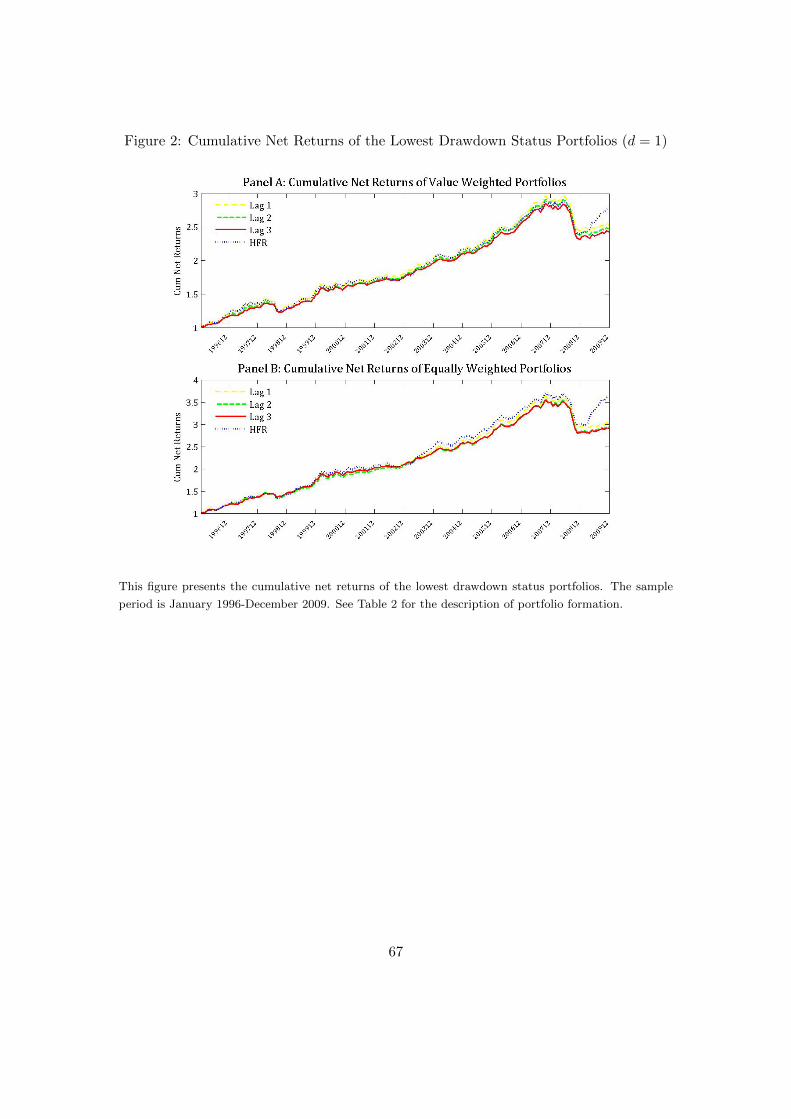
Figure 2: Cumulative Net Returns of the Lowest Drawdown Status Portfolios (d = 1)
This figure presents the cumulative net returns of the lowest drawdown status portfolios. The sample
period is January 1996-December 2009. See Table 2 for the description of portfolio formation.
67

Figure 3: Cumulative Net Returns of the Highest Drawdown Status Portfolios (d = 10)
This figure presents the cumulative net returns of the highest drawdown status portfolios. The sample
period is January 1996-December 2009. See Table 2 for the description of portfolio formation.
68

Figure 4: Stop Reporting and Liquidation of Funds in the Portfolios
Panel A of this figure presents the average number of consecutive years that a fund that stops reporting
during the portfolio formation period stays in the d = 1 decile. Panel B of this figure presents the average
number of consecutive years that a fund that is liquidated during the portfolio formation period stays
in the d = 10 decile. The sample period is 1996-2009.
69

Figure 5: Flows of Surviving vs. Liquidating Funds
This figure plots the time series of the average 12-month lagged flows –excluding the flows of the liqui-
dation month– of the portfolio of funds in the 3-lag highest drawdown decile (surviving funds) vs. the
portfolio of funds in the 3-lag highest drawdown status portfolio that are liquidated (liquidating funds).
There are no liquidated funds in the latter portfolio during 1996-1997. Hence, the sample period of
comparison is 1998-2009.
70

Figure 6: Managerial Ownership in Surviving Funds
Panel A of this figure plots the time series of managerial ownership of the portfolio of funds in the 3-lag
high drawdown status portfolio. Panel B plots the fraction of funds in the lag 3 large-drawdown status
portfolio that have a managerial ownership below 50%. The sample period is 1996-2009.
71