On the Dynamics of Glassy Systems

by

Le Yan

A dissertation submitted in partial fulfillment

of the requirements for the degree of

Doctor of Philosophy

Department of Physics

New York University

September 2015

Matthieu Wyart

arX

iv:1

604.

0308

7v1

[co

nd-m

at.d

is-n

n] 1

1 A

pr 2

016

© Le YanAll Rights Reserved, 2015

Dedication

To my mother.

iv

Acknowledgements

First of all, I would like to thank my advisor, Matthieu Wyart, for his

mentoring and guidance in science and in career. His deep insight into the phys-

ical world always enlightens me and leads to the right way to solve the scientific

problems. I would like to thank Markus Muller, for his thoughtful direction in

our collaboration on the spin glass project. I would like to thank my dissertation

committee of Alexander Grosberg, David Pine, Paul Chaikin and Daniel Stein for

their helpful suggestions on both science and career. I would also like to acknowl-

edge all other principal investigators in the Center for Soft Matter Research at

NYU, David Grier, Jasna Brujic, Marc Gershow and Alexandra Zidovska, for their

discussions and comments that helped me make better science.

It was a great pleasure to work in the Center for Soft Matter Research,

and I want to thank all current and former members for their support over the

past four years. In particular, I want to thank, Gustavo During, Edan Lerner,

Eric DeGiuli and Jie Lin in Wyart’s group, Marco Baity-Jesi, Antoine Barizien

and Alexis Front visited to the group, collaborations with whom are extremely

pleasant and enthusiastic; Lang Feng, who introduced me to the Center; Payam

Rowghanian, Jan Smrek, and Cato Sandford, who created a casual atmosphere in

v

the office room we shared and taught me a lot in language and culture; and Yin

Zhang, Chen Wang, Wenhai Zheng, and Guolong Zhu, who continually “bothered”

me with their research problems.

Last but not least, I am thankful to all my friends who helped me and

encouraged me in my life at New York University, without whom I could not finish

my Ph. D. study. Especially, I want to thank, Yanchao Xin, Hong Zhang, Shuang

Li, and Yuqian Liu, who were my roommates and closest friends in New York; Tao

Jiang, Lan Gong, and Hongliang Liu, who guided me as senior Ph. D. students;

and Patrick Cooper, Daniel Foreman-Mackey, Victor Gorbenko, Shahab Kohani,

Henrique Moyses, and Stefano Storace, who are my same-year fellows survived in

the end.

vi

Preface

Life is transient. What should we do in our limited time to make some

differences? Some figures, like Euclid, are “alive” in people’s minds even after

thousands of years, because their masterpieces keep inspiring and benefiting people.

Knowledge of nature and ourselves is a wealth of all mankind, a contribution to

which would surely make my life meaningful. That is my initial motivation for

doing science.

Followed a typical education path, I became a Ph. D. student at New

York University, standing at the gate to my research career dream and looking for

questions that I could make use of my lifetime to work on. Fortunately, I met my

second mentor (after my father as the first), Matthieu Wyart. He introduced me

to the question of transients in nature – the dynamics of glassy systems.

“The flying arrow is motionless”, the famous paradox of ancient Greek

philosopher Zeno, has a similar modern version in the physics of glasses: “the

flowing liquid is solid”. Zeno’s paradox is deeply related to calculus and the con-

cept of limit, nonetheless, the physics lying behind the glass connects to a long

dynamical time scale. Below the time scale, a glass appears to be static and solid,

while above, it flows as a sticky liquid, like honey. It is also a physical phenomenon

closely related to life. Imagine you are stuck in a traffic jam: if you are in a hurry,

staring at the second hand on your watch, you may probably curse the jammed

traffic; but if you are relaxed, enjoying the music and the views, you may hap-

pily drive to your destination after momentary waitings. These dynamical systems

characterized by long time scales are glassy systems.

vii

In glassy materials, the dynamical time scale can be tuned by temperature

and driving forces like gravity. For example, the wax flows more and more easily

if one heats it up; the sandpile slides faster and faster when the bed of the dump

truck is tilted more and more steeply. However, how the time scale depends on

temperature and driving force may vary from system to system, and there are not

yet universal rules like Newton’s Laws to describe different dynamics. We are curi-

ous to know what determines the dynamical properties of the glassy systems from

microscopic level; Is there any dynamical universality among systems that possess

certain microscopic features? One prominent concept of dynamical systems is self-

organization: the trend that the system spontaneously evolves to states where the

dynamical time scale diverges. So the dynamical transitions are usually relevant

in glassy systems. The dynamics in this situation become rich: phenomena of all

different time scales accompanied with different sizes appear. For example, in the

Earth crust as a glassy system, earthquakes varying in intensity from unnoticeable

to devastating can happen. But how our nature spontaneously evolves to these

critical states is still lack of a mathematical description.

I have studied these general questions in specific systems and models dur-

ing my Ph. D. and conclude them in this dissertation. The dissertation may never

be eternal, but to me, it is a first small but important step towards my scientific

career, which, I hope, will leave some valuable thoughts that continually inspire

and benefit others.

viii

Abstract

Glassy systems are disordered systems characterized by extremely slow

dynamics. Examples are supercooled liquids, whose dynamics slow down under

cooling. The specific pattern of slowing-down depends on the material considered.

This dependence is poorly understood, in particular, it remains generally unclear

which aspects of the microscopic structures control the dynamics and other macro-

scopic properties. Attacking this question is one of the two main aspects of this

dissertation. We have introduced a new class of models of supercooled liquids,

which captures the central aspects of the correspondence between structure and

elasticity on the one hand, the correlation of structure and thermodynamic and

dynamic properties on the other. These models can also be resolved analytically,

leading to theoretical insights into the question. Our results also shed new light on

the temperature-dependence of the topology of covalent networks, in particular,

on the rigidity transition that occurs when the valence is increased. Observations

suggested the presence of a nearly critical range in the proximity of the rigidity

threshold. Our work rules out the predominant explanation for this phenomenon

by a “rigidity window” where the rigidity is barely satisfied.

Other questions appear in glassy systems at zero temperature, when the

thermal activation time is infinitely long. In that situation, a glassy system can flow

if an external driving force is imposed above some threshold. Near the threshold,

the dynamics are critical. To describe the critical dynamics, one must understand

how the system self-organizes into specific configurations.

The first example we will consider is the erosion of a river bed. Grains

or pebbles are pushed by a fluid and roll on a disordered landscape made of the

ix

static particles. Experiments support the existence of a threshold forcing, below

which no erosion flux is observed. Near the threshold, the transient state takes

very long and the flux converges very slowly toward its stationary value. In the

field, this long transient state is called “armoring” and corresponds to the filling

up of holes on the frozen landscape by moving particles. The dynamics near

the threshold are relevant for geophysical applications – gravel river beds tend to

spontaneously sit at the threshold where erosion stops, but are poorly understood.

In this dissertation, we present a novel microscopic model to describe the erosion

near threshold. This model makes new quantitative predictions for the erosion flux

vs the applied forcing and predicts that the spatial reparation of the flux is highly

non-trivial: it is power-law distributed in space with long range correlation in the

flux direction, but no correlations in the perpendicular directions. We introduce a

mean-field model to capture analytically some of these properties.

To study further the self-organization of driven glassy systems, we inves-

tigate, as our last example, the athermal dynamics of mean-field spin glasses. Like

many of other glasses, such as electron glasses, random close packings, etc., the

spin glass self-organizes into the configurations that are stable, but barely so. Such

marginal stability appears with the presence of a pseudogap in soft excitations –

a density of states vanishing as a power-law distribution at zero energy. How such

pseudogaps appear dynamically as the systems are prepared and driven was not

understood theoretically. We elucidate this question, by introducing a stochastic

process mimicking the dynamics, and show that the emergence of a pseudogap is

deeply related to very strong anti-correlations emerging among soft excitations.

x

Contents

Dedication iv

Acknowledgements v

Preface vii

Abstract ix

List of Figures xiv

List of Appendices xxvii

1 Introduction 1

1.1 Dynamics under cooling – glass transition . . . . . . . . . . . . . . 4

1.2 Rigidity of a structure . . . . . . . . . . . . . . . . . . . . . . . . . 8

1.3 Non-equilibrium dynamical phase transition . . . . . . . . . . . . . 15

1.4 Critical dynamics . . . . . . . . . . . . . . . . . . . . . . . . . . . . 19

1.5 Structure of the dissertation . . . . . . . . . . . . . . . . . . . . . . 23

2 Why glass elasticity affects the thermodynamics and fragility of

super-cooled liquids 25

xi

2.1 Introduction . . . . . . . . . . . . . . . . . . . . . . . . . . . . . . . 26

2.2 Random Elastic Network Model . . . . . . . . . . . . . . . . . . . . 29

2.3 Numerical Results of the Model . . . . . . . . . . . . . . . . . . . . 33

2.4 Theory on Thermodynamics of the Model . . . . . . . . . . . . . . 39

2.5 Discussion . . . . . . . . . . . . . . . . . . . . . . . . . . . . . . . . 45

3 Evolution of Covalent Networks under Cooling: Contrasting the

Rigidity Window and Jamming Scenarios 47

3.1 Introduction . . . . . . . . . . . . . . . . . . . . . . . . . . . . . . . 48

3.2 Adaptive Elastic Network Model . . . . . . . . . . . . . . . . . . . . 50

3.3 Numerical Proofs of the Mean-field Rigidity Transition . . . . . . . 53

3.4 A Simple Argument for the Mean-field Scenario . . . . . . . . . . . 58

4 Adaptive Elastic Networks as Models of Supercooled Liquids 61

4.1 Introduction . . . . . . . . . . . . . . . . . . . . . . . . . . . . . . . 62

4.2 Adaptive Network Model . . . . . . . . . . . . . . . . . . . . . . . . 66

4.3 Numerical Results of the Model . . . . . . . . . . . . . . . . . . . . 70

4.4 Theory of Thermodynamics . . . . . . . . . . . . . . . . . . . . . . 76

4.5 Conclusions . . . . . . . . . . . . . . . . . . . . . . . . . . . . . . . 84

5 A Model for the Erosion Onset of a Granular Bed Sheared by a

Viscous Fluid 86

5.1 Introduction . . . . . . . . . . . . . . . . . . . . . . . . . . . . . . . 87

5.2 Erosion Model . . . . . . . . . . . . . . . . . . . . . . . . . . . . . . 89

5.3 Numerical Results on Dynamics of the Model . . . . . . . . . . . . 92

5.4 An Argument on the Scaling Relation . . . . . . . . . . . . . . . . . 97

5.5 Mean-field Model on the Distribution of Local Currents . . . . . . . 98

xii

5.6 Potential Experimental Tests . . . . . . . . . . . . . . . . . . . . . 99

6 Dynamics and Correlations among Soft Excitations in Marginally

Stable Glasses 101

6.1 Introduction . . . . . . . . . . . . . . . . . . . . . . . . . . . . . . . 102

6.2 Dynamics of Sherrington-Kirkpatrick Model . . . . . . . . . . . . . 104

6.3 Multi-spin Stability Criterion . . . . . . . . . . . . . . . . . . . . . 106

6.4 Fokker-Planck Description of the Dynamics . . . . . . . . . . . . . . 109

6.5 Emergence of Correlations . . . . . . . . . . . . . . . . . . . . . . . 111

6.6 Conclusion . . . . . . . . . . . . . . . . . . . . . . . . . . . . . . . . 114

7 Outlooks 115

7.1 Intermediate Phase . . . . . . . . . . . . . . . . . . . . . . . . . . . 115

7.2 Dynamical Transition at Finite Temperature . . . . . . . . . . . . . 118

7.3 Universality of Critical Dynamics . . . . . . . . . . . . . . . . . . . 120

8 Conclusion 125

Appendices 128

Bibliography 164

xiii

List of Figures

1.1 A phase diagram of static and dynamic phases of glassy systems. T is

the temperature, f is the driving force. . . . . . . . . . . . . . . . . . 2

1.2 Scatter plot of the jump of specific heat ∆Cp/∆Sm and the fragility m of

different glassy materials. The dashed line is given by m = 40∆Cp/∆Sm,

where ∆Sm is the entropy gain in melting of the same material. The plot

is reproduced from Reference [5]. . . . . . . . . . . . . . . . . . . . . 5

1.3 Scatter plot of boson peak intensity ratio R1 and fragility m of different

glasses. The plot is reproduced from Reference [33]. . . . . . . . . . . 7

1.4 The fragility m (Left) and the jump of specific heat ∆cp (Right) of chalco-

genides with coordination number r. The plots are reproduced from

References [4, 35]. . . . . . . . . . . . . . . . . . . . . . . . . . . . . 7

1.5 An illustration of the rigidity transition of a network by adding pairwise

constraints from floppy (Left) to isostatic (Middle) and to self-stressed

(Right). . . . . . . . . . . . . . . . . . . . . . . . . . . . . . . . . . 9

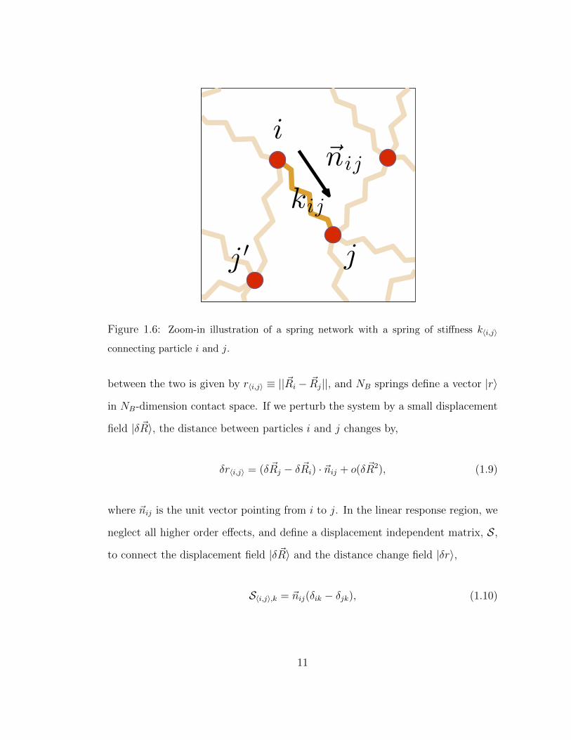
1.6 Zoom-in illustration of a spring network with a spring of stiffness k〈i,j〉

connecting particle i and j. . . . . . . . . . . . . . . . . . . . . . . . 11

xiv

1.7 Particle trajectories (top view) of a granular bed erosion driven by water

flow. The water is injected from the left to right, as indicated by the

blue arrow. The plot is reproduced from Reference [83]. . . . . . . . . 16

1.8 Pseudogap in distribution of local stabilities in various glassy systems.

(a) Density of states P (E) in Coulomb glasses, where the gap is centered

at the Fermi level; (b) Distribution of local fields P (λ) in spin glasses;

(c) Distribution of contact forces p(f) and (d) distribution of contact

gaps g(h) in packings of hard spheres. The plots are reproduced from

References [104, 109, 112]. . . . . . . . . . . . . . . . . . . . . . . . . 21

1.9 Illustration of the evolution of a dynamical system from unstable states

to the margin of the stable states in the phase space. A and B are

arbitrary coordinates of the phase space. The plot is reproduced from

Reference [101]. . . . . . . . . . . . . . . . . . . . . . . . . . . . . . 23

2.1 Top row: sketches of covalent networks with different mean valence r

around the valence rc: red solid lines represent covalent bonds; cyan

dash lines represent van der Waals interactions. Bottom: sketch

of our elastic network model with varying coordination number z

(defined as the average number of strong springs in red) around

Maxwell threshold zc; cyan springs have a much weaker stiffness,

and model weak interactions. . . . . . . . . . . . . . . . . . . . . . 30

xv

2.2 Specific heat c(T ) v.s. rescaled temperature T/Tg for various excess

coordination δz ≡ z − zc as indicated in legend, for α = 3 × 10−4

and d = 2. c(T ) displays a jump at the glass transition. Solid lines

are theoretical predictions, deprived of any fitting parameters, of

our mean-field approximation. They terminate at the Kautzman

temperature TK . Inset: glass transition temperature Tg vs δz for

several amplitude of weak interactions α, as indicated in legend. . 35

2.3 Jump of specific heat ∆c versus excess coordination δz in d = 2 for

different strength of weak springs α, as indicated in legend. Solid

lines are mean-field predictions not enforcing the orthogonality of

the |δrp〉, dashed-line corresponds to the ROM where orthogonal-

ity is enforced. In both cases the specific heat is computed at the

numerically obtained temperature Tg. Inset: theoretical predictions

for ∆c vs δz computed at the theoretical temperature TK . . . . . . 36

2.4 Fragility m versus excess coordination δz for different strength of

weak interactions α as indicated in legend, in d = 2. Dash dot lines

are guide to the eyes, and reveal the non-monotonic behavior of m

near the rigidity transition. Inset: Angell plot representing log τ

v.s. inverse temperature Tg/T for different δz and α = 3× 10−4. . 38

2.5 Left: Inverse boson peak amplitude R1 versus excess coordination

δz in our d = 3 elastic network model, for different weak interaction

strenghts as indicated in legend. Dash dot lines are drawn to guide

one’s eyes. Right: Inverse boson peak amplitude R1 versus fragility

m for different weak springs α. . . . . . . . . . . . . . . . . . . . . . 41

xvi

3.1 Three distinct scenarios for the rigidity transition in chalcogenide glasses.

Bonds in blue, green, red corresponds respectively to floppy (under-

constrained), isostatic (marginally-constrained) and over-constrained re-

gions. p(z) is the probability that a rigid cluster (made of green and red

bonds) percolates, as a function of the valence z. (a) Rigidity percola-

tion model where bonds are randomly deposited on a lattice. Percolation

occurs suddenly and p(z) jumps from 0 to 1 at zcen < zc. At zcen, the

rigid network is fractal. (b) The self-organizing network model at zero

temperature. Over-constrained regions are penalized energetically and

are absent for z < zz. For z ∈ [ziso, zc], 0 < p(z) < 1 even in the thermo-

dynamic limit. (c) Mean-field scenario, where p(z) jumps from 0 to 1 at

zc, and where the rigid cluster at zc is not fractal. . . . . . . . . . . . . 51

3.2 Illustration of our model. The triangular lattice is slightly distorted

as shown in the inset of (a), and weak springs connecting all second

neighbors are present, as shown in blue in the inset of (b). Our Monte-

Carlo considers the motion of strong springs such as that leading from

(a) to (b). . . . . . . . . . . . . . . . . . . . . . . . . . . . . . . . . 52

3.3 P∞ vs (z−zc)N1/dν in the weak-force condition (a) and for T =∞ (b). p

vs δz ≡ z − zc in the weak-force (c) and strong-force (d) conditions. The

black squares are extrapolations of the finite N spline curves, as detailed

in the main text. In (c), the gray line is a step function at z = zc, whereas

in (d) it corresponds to the result of [75]. . . . . . . . . . . . . . . . . 54

xvii

3.4 D(ω) at z − zc = −0.05 and various T indicated in legend for (a) α = 0

and (b) α = 0.0003. Gray dashed lines are numerical solution of mean-

field networks generated in [130]. (c) Boson peak frequency ω∗ vs coor-

dination z for the weak-interaction regime. ω∗ is defined as the peak

frequency of D(ω)/ωd−1, a quantity shown in (d). . . . . . . . . . . . . 56

3.5 Shear modulus of the strong network G vs δz ≡ z − zc for parameters

indicated in legend. The total shear modulus Gtot including the effect of

weak springs is represented for the weak-interaction regime. Inset: same

plot in log-log scale, the horizontal axis is z − zc for low-temperatures

conditions (blue and green), and z − zcen at T =∞ (red). . . . . . . . . 57

4.1 Illustration of rigidity transition. Blue, green, and red color the floppy,

isostatic, and stressed clusters, respectively. . . . . . . . . . . . . . . . 64

xviii

4.2 (Color online) (a) and (b) Illustration of the frozen network model [116];

(c) and (d) illustrate the adaptive network model [117]. In the latter

case, the triangular lattice is systematically distorted in a unit cell of

four nodes shown in the inset of (c). We group nodes by four, labeled

as, A, B, C, and D in Fig. 4.2. One group forms the unit cell of the

crystalline lattice. Each cell is distorted identically in the following way:

node A stays, while nodes B, C, and D move by a distance δ, B along the

direction perpendicular to BC, C along the direction perpendicular to

CD, and D along the direction perpendicular to DB. δ is set to 0.2 with

the lattice constant as unity. Weak springs connecting (b) six nearest

neighbors without strong springs and (d) six next-nearest-neighbors are

indicated in straight cyan lines, emphasized for the central node. (c)

Illustration of an allowed step, where the strong spring in red relocates

to a vacant edge indicated by a dashed blue line. . . . . . . . . . . . . 67

4.3 (Color online) Illustration of configuration energy of the adaptive network

model (δz = 0.27). Solid lines are springs, colored according to their

extensions: from red to purple, the springs go from being stretched to

being compressed, with spring extensions shown in the unit of ε. Left:

Nodes sit at lattice sites, so the color shows the rest length mismatches

of the springs εγ. Right: Nodes are relaxed to mechanical equilibrium.

Most links appear in green, indicating that most of the elastic energy is

released. The configuration energy is defined by the residual energy. . . 68

4.4 (Color online) Relaxation time τ in log-scale versus inverse temperature

1/T for different coordination numbers δz and α = 0.0003. The solid

black line indicates a power law relation between τ and T : τ ∼ T−1/2. . 71

xix

4.5 (Color online) Left: Shear modulus of adaptive networks at tempera-

ture T rescaled by G at T = ∞ G(z, T )/G(z,∞), α = 0.0003. The

temperature T is rescaled by Tg. Right: Correlation between transition

temperature Tg and shear modulus G in the frozen network model [116]. 72

4.6 (Color online) Thermodynamics of the adaptive network model without

weak constraints α = 0. (a) Energy E/Ns vs. temperature; (b) specific

heat C/Ns vs. temperature; (c) excess number density of redundant con-

straints nex extracted using the pebble game algorithm vs. temperature.

Symbols are numerical data; solid lines are theoretic predictions. . . . . 74

4.7 (Color online) Top: Specific heat c(z, T ) vs scaled temperature T/Tg for

networks with average coordination numbers near and away from the

isostatic on both floppy and rigid sides. The strength of the weak con-

straints is given by α = 0.0003. Bottom: Specific heat at temperature Tg,

c(z, Tg), vs coordination number δz for α = 0, 0.0003, 0.003, 0.03. The

inset shows the transition temperature Tg for different z and α. Sym-

bols are numerical results, and lines are theoretical predictions: dashed

lines are for frozen network model and solid lines are for the new model

derived in section IV. . . . . . . . . . . . . . . . . . . . . . . . . . . . 75

4.8 (Color online) Theoretical predictions for the jump of specific heat. For

vanishingly weak springs α → 0, it is predicted that the jump is essen-

tially constant for z < zc and then drops to zero a zc. For larger z, it

behaves as z − zc. As α grows this sharp curve becomes smooth, but a

minimum is still present near z = zc. . . . . . . . . . . . . . . . . . . 77

xx

4.9 (Color online) (a) z < zc, localized redundant constraints (red) in a

floppy sea (blue); (b) z > zc localized floppy modes (blue) in a rigid sea

(red and green). . . . . . . . . . . . . . . . . . . . . . . . . . . . . . 79

4.10 (Color online) Left: Excess number density of redundant constraints

nex(z, β). Right: Fluctuation of the number density of redundant con-

straints (∆nr)2. The solid black lines show the predictions from the

approximate entropy Eq.(4.9). . . . . . . . . . . . . . . . . . . . . . . 81

5.1 Illustration of the model. Small circles indicate lattice sites, particles

are represented by discs in yellow, or green if motion occurred between t

(left) and t+1 (right). The black arrow is in the downhill direction. Solid

lines indicate outlet with positive forces. If a particle has two outlets with

positive forces, the larger (smaller) one is colored in red (blue). . . . . 91

5.2 Average current J versus θ−θc in log-log scale for the (a) “equilibrated”

and (b) “quenched” protocols, for which θc = 0.164 ± 0.002 and θc =

0.172±0.002 respectively- a difference plausibly due to finite size effects.

The black solid lines with slope one indicate the linear relation J ∝ θ−θc.

(c) Density of conducting sites ρs versus θ − θc for the “equilibrated”

protocol. (d) ρs curves collapsed by rescaling θ − θc with L1/ν , where

ν = 3.0± 0.2. . . . . . . . . . . . . . . . . . . . . . . . . . . . . . . 92

5.3 Left: Transient time tconv v.s. θ. For a given realization, tconv is defined

as the smallest time for which J(t) − J ≤√V ar(J) where V ar(J) =

limT→∞1T

∑Tt=1(J(t)−J)2. The gray dashed lines correspond to tconv ∼

|θ − θc|−2.5. Right: The obtained exponent fits well the observations of

[88]. . . . . . . . . . . . . . . . . . . . . . . . . . . . . . . . . . . . 94

xxi

5.4 Examples of drainage pattern just below θc (Left) and above (Right).

The black arrow shows the downhill direction. The thickness of the lines

represents σi→j in logarithmic scale. A few examples showing splitting

events are magnified on the left. Here W = 45 and L = 128, and J > 0

even below θc due to finite size effects. . . . . . . . . . . . . . . . . . . 95

5.5 Distribution of the site current P (σ) in steady state for given average

currents J of (a) the erosion model (L = 256, W = 64) and (b) our

mean-field model (W = 1600). . . . . . . . . . . . . . . . . . . . . . . 96

5.6 (a) Transverse current correlations CT at θc and (b) longitudinal current

correlation CL at θc and at θ − θc = 0.25 for L = 256 (dashed line). . . . 96

6.1 (a) Hysteresis loop: Magnetization M under a periodic quasi-static driv-

ing of the external field h. Inset: magnified segment of the hysteresis

loop of a finite size system. (b) Distribution of local stabilities, ρ(λ), in

locally stable states along the hysteresis loops for different system sizes

N . (c) Finite size scaling of the avalanche size distribution D(n) con-

firms τ = σ = 1 up to logarithmic corrections. (d) Correlation C(λ)

between the least stable spin and spins of stability λ in locally sta-

ble states along the hysteresis loop. The data for different system sizes

collapses, implying C(λ 1) ∼ 1/λ in the thermodynamic limit. . . . . 106

6.2 (a) The average dissipated energy ∆H in avalanches of size n scales as

∆H ∼ n lnn/√N . −∆H/n is a measure of the typical value of the

stability of most unstable spins, λ0(n). Thus, in the thermodynamic

limit, λ0 ∼ lnn/√N 1 even for very large avalanches. (b) The

average number of times, F (n), spins active in avalanches of size n re-flip

later on in the avalanche. . . . . . . . . . . . . . . . . . . . . . . . . . 107

xxii

6.3 Illustration of a step in the dynamics, in the SK model and the random

walker model. Circles on the λ-axis represent the spins or walkers. At

each step, the most unstable spin (in red) is reflected to the stable side,

while all others (in green or blue) receive a kick and move. The dashed

and solid line outlines the density profile ρ(λ) ∼ λ for λ > 1/√N . The

blue spins were initially frustrated with the flipping spin 0. They are

stabilized and are now unfrustrated with 0. In contrast, green spins

become frustrated with spin 0 and are softer now. Because of the motion

of spins depends on their frustration with spin 0, a correlation builds up

at small λ, leading to an overall frustration of “soft” spins among each

other. . . . . . . . . . . . . . . . . . . . . . . . . . . . . . . . . . . . 111

7.1 Boson peak frequency ω∗ obtained from equilibrated configurations near

Tg vs coordination number δz for different α. . . . . . . . . . . . . . . 116

7.2 (a) (b) Avalanche size distribution D(n); (c) (d) Magnetization jump

distribution P(S). (a) (c) Reluctant dynamics; (b) (d) Greedy dynamics. 121

7.3 (a) Average avalanche size 〈n〉 (b) Average magnetization jump 〈S〉 of

avalanches. . . . . . . . . . . . . . . . . . . . . . . . . . . . . . . . . 122

7.4 Illustration of the dynamic model. Circles on the axis represent the

walkers. The leaping walker (in red) jumps to the stable side, and other

walkers (in blue) move random steps according to Eq.(7.4). . . . . . . . 123

7.5 (a) (c) Distribution of local stability ρ(λ) in stable states and (b) (d)

Distribution of avalanche size D(n) scaled by finite size N for (a) (b) SK

model and (c) (d) random walker model. In the pseudo-gap near λ = 0,

ρ(λ) ∝ λ in both (a) and (c). The collapses in (b) and (d) indicate the

power law exponent τ = 1.0, and σ = 1 with a logarithmic correction. . . 124

xxiii

A.1 Squares show the shear modulus G normalized by its value at the

rigidity threshold for Ge-Se, taken from Ref. [36]. Circles show G

for Ge-Sb-Se, taken from Ref. [37]. Lines display the shear modulus

G for network models in d = 3 using different α, as indicated in the

legend. . . . . . . . . . . . . . . . . . . . . . . . . . . . . . . . . . . 131

A.2 Angell plot representing log τ v.s. inverse temperature Tg/T for

different δz and two system sizes N = 64 and N = 256, α = 0.0003. 135

B.1 Illustration of distortion of the triangular lattice, performed to re-

move straight lines. . . . . . . . . . . . . . . . . . . . . . . . . . . . 141

B.2 Fluctuations of coordination 〈(z − z)2〉 vs temperature T for different α

as indicated in legend. The network size is N = 256 and the block size is

N∗ = 64. Mean coordination number corresponds to a) z− zc = −0.383,

b) z − zc = −0.055, c) z − zc = 0.523. . . . . . . . . . . . . . . . . . . 143

B.3 Boson peak frequency ω∗ as a function of excess coordination δz = z−zc

for different α as indicated in legend, at temperatures T = α. ω∗ = 0

indicates that no maximum was observed in D(ω)/ωd−1, consistent with

the presence of fractons at very low frequency. . . . . . . . . . . . . . . 145

C.1 Variation of density of states D(ω, T ) with temperature for the same

z = −0.055, α = 0.0003. Left: density of states in log-log scale. Right:

density of states normalized by its T = ∞ value, emphasizing its differ-

ence under cooling. Inset: participation ratio P (ω, T ) variation under

cooling. . . . . . . . . . . . . . . . . . . . . . . . . . . . . . . . . . 148

xxiv

C.2 Density of states D(ω, T ) for adaptive networks with different z. (a) Ran-

dom diluted networks T = ∞; a power law D(ω) ∼ ω−0.25 is shown in

low frequency range for networks near zcen. (b) Adaptive networks with-

out weak constraints (α = 0) at T = 0.0003; power laws with different

exponents are shown for networks in the rigidity window: D(ω) ∼ ω−0.25

for δz = −0.055, D(ω) ∼ ω−0.5 for δz = 0.0. (c) Adaptive networks

with weak constraints (α = 0.0003) at T ≈ α; away from isostatic, den-

sity of states are gapped between zero frequency and Boson peak, where

D(ω) ∼ ω0. Inset (d) Participation ratio P (ω, T ) at T =∞, see text for

definition. . . . . . . . . . . . . . . . . . . . . . . . . . . . . . . . . 149

C.3 Vector plots of vibrational modes in randomly diluted networks, N =

100 × 100. (a) A typical Debye mode, δz = 0.501, ω = 0.017. (b) A

typical anomalous mode on boson peak, δz = −0.049, ω = 0.011. (c) A

typical fracton, δz = −0.049, ω = 0.0007. . . . . . . . . . . . . . . . . 151

C.4 Correlation between a low frequency fractal mode and isostatic clusters.

A network configuration (δz = −0.042) is shown with its springs in the

over-constrained regions colored in red, in the isostatic regions colored

in green, and in the floppy regions colored in blue. A typical fracton

(ω = 5× 10−4) specified in this configuration is plotted on top. . . . . 154

D.1 Histogram of excitations with given energy change ∆H for different

metastable states along the hysteresis curve, m = 8, m′ = 16, and

N = 3000. . . . . . . . . . . . . . . . . . . . . . . . . . . . . . . . . 157

xxv

D.2 The lower data set in solid lines is the total energy ∆H(n) dissipated

in avalanches of size n. The upper data set in dashed lines is the

sum of local stabilities (before the avalanche) of spins that are going to

flip in the avalanche,∑

iflip λi. This shows that the dissipated energy is

vanishingly small as compared to the naıve sum over local stabilities, as

n→∞, since the two curves scale as different power laws with n. . . . 159

D.3 Left: the quantity NC(λ, λ′)√

(λ+ c(N))2 + (λ′ + c(N))2 is numerically

computed for various λ and λ′, and behaves nearly as a constant (as the

color code indicates, this quantity only changes by a factor 3 in the entire

range considered. Right: Correlation C(λ, λ′), for λ′ = 5λ with different

system sizes N and for different directions λ′ = aλ, a = 0, 1, 2, 5 with

N = 5000. . . . . . . . . . . . . . . . . . . . . . . . . . . . . . . . . 160

xxvi

List of Appendices

A Why glass elasticity affects the thermodynamics and fragility of super-

cooled liquids? . . . . . . . . . . . . . . . . . . . . . . . . . . . . . . 129

B Evolution of covalent networks under cooling . . . . . . . . . . . . . . 140

C Adaptive elastic networks as a model for supercooled liquids . . . . . . 146

D Dynamics and correlations among soft excitations in marginally stable

glasses . . . . . . . . . . . . . . . . . . . . . . . . . . . . . . . . . . 155

xxvii

Chapter 1

Introduction

Statistical physics, one of the cornerstones of modern physics and chem-

istry, sets the theoretical framework to describe systems in thermal equilibrium.

However, more often, systems are not equilibrated. This is the case for open sys-

tems which receive energy fluxes from their environments, such as the living or

social systems. Other examples are glassy systems, whose thermal activation time

is so long that they cannot equilibrate on practical time scales. Examples are

the structural glasses that make our windows, whose dynamics are dominated by

a glass transition between an equilibrated liquid state and an out-of-equilibrium

glass state with an extremely long relaxation time. Other examples are granular

materials, where the temperature effect is too small to be relevant. These sys-

tems are yield stress materials, which can flow if a sufficient forcing is applied.

The transition between the solid and liquid phases is a non-equilibrium dynamical

transition. The two transitions are represented in the phase diagram in Fig. 1.1.

Understanding them is a long-standing topic of soft condensed matter physics.

1

Staticf

TGlass Transition

Granular Flow

Transition

Dynamic

Figure 1.1: A phase diagram of static and dynamic phases of glassy systems. T is the

temperature, f is the driving force.

The thermal relaxation of a liquid can be enormously prolonged under

cooling [1, 2]. Classical examples are structural glasses, which can be elegantly

shaped by blowing them. Blowing is possible because these materials are very

viscous and flow on the scale of seconds near the glass transition, compared with

picoseconds in liquid phase at high temperature. In light of the long history of

glass manufacture [3], it is surprising how little is understood of the microscopic

cause for their slow dynamics.In particular, the specific pattern of slowing down

near the glass transition depends on the material considered [4, 5]. There is no

theoretical framework to predict that dependence.

At zero temperature, the thermal activation time of a glassy system is

2

absent. The system can however transition from a static state to a dynamic flow-

ing state once a sufficient external forcing is applied. For instance, rocky river

beds and sand dunes can flow when pebbles and sand grains are eroded by the

water flow and the wind respectively [6]. Many experiments support that erosion

occurs only when the stress applied by the fluid exceeds a threshold. Understand-

ing this threshold is important for geophysical applications, as river beds tend to

spontaneously evolve toward this threshold where erosion stops [7, 8]. No com-

pelling theoretical framework has been proposed to describe the dynamics near

the threshold. One interesting effect is the “armoring” phenomenon: near the

threshold, there are long transients where the average number of mobile particles

flowing above the frozen bed slowly decays. This slow decay corresponds to the

filling up of holes by mobile particles: the system self-organizes into configurations

where a minimal number of particles remain mobile.

Another kind of self-organization occurs in glassy systems at zero tem-

perature, when interactions are effectively long-range. Examples include electron

glasses, spin glasses or packings of hard particles where elastic interactions domi-

nate. Such systems spontaneously self-organize into configurations that are stable,

but barely so. As a consequence, rich dynamics occur when a perturbation is ap-

plied. Typical examples are Barkhausen noises in magnetic spin systems [9–11] and

avalanches in sand and snow packings. Currently, we lack a dynamical description

of how the marginality is reached in these systems.

3

1.1 Dynamics under cooling – glass transition

A glass is a solid which forms when a supercooled liquid – a liquid at a

temperature below its melting point – falls out of equilibrium under cooling. In the

practical sense, glass transition is essentially different from other equilibrium phase

transitions, where the two phases are both in thermal equilibrium and the tran-

sition is determined by symmetry breaking [12, 13]. For example, the translation

invariant symmetry breaks in crystallization [12]. By contrast, no obvious symme-

try is found broken in the glass transition problem. So there is no comparable

theory based on symmetry explaining the glass transition.

The most significant features of glasses are their extremely slow dynamics,

which appear to be associated with collective behaviors characterized by a increas-

ing correlation length of the dynamics [14–18]. This increase is however moderate,

since the size of collectively rearranging regions in a liquid increases only by four

to five times, in contrast to a 1016-fold growth in the relaxation time [1, 2, 19–23].

Experimentalists often fit this fast rise of the relaxation time by the Vogel-Fulcher-

Tammann law [24–26],

τ(T ) = τ0 exp

(A

T − T0

), (1.1)

where τ0, A and T0 are fitting parameters for different materials. The exponential

form, Eq.(1.1), indicates that the dynamics in glasses slow down much faster than

a typical thermal activation process, where the relaxation time is captured by

Arrhenius law:

τ(T ) ∝ exp

(∆F

T

), (1.2)

where ∆F is the free energy barrier of relaxation. The two formulas are consistent

4

only if the free energy barrier ∆F depends on temperature and becomes singular

at T0. In most fragile liquids, this ∆F can increase by 6 to 7 fold under cooling.

Figure 1.2: Scatter plot of the jump of specific heat ∆Cp/∆Sm and the fragility m

of different glassy materials. The dashed line is given by m = 40∆Cp/∆Sm, where

∆Sm is the entropy gain in melting of the same material. The plot is reproduced from

Reference [5].

Experiments reveal a connection between the dynamics and thermody-

namics in supercooled liquids. For instance, the jump of specific heat ∆cp and

the fragility m are linearly correlated for different kinds of glass-forming materials,

ranging from network to polymer glasses, as shown in Fig. 1.2 [5, 27]. The fragility,

characterizing the temperature dependence of the relaxation time in different ma-

terials, is defined as,

m ≡ ∂ ln τ(T )/τ0

∂(T/Tg)

∣∣∣∣T=Tg

= lnτ(Tg)

τ0

− ∂∆F (T )

∂T

∣∣∣∣Tg

. (1.3)

5

The liquids following the Arrhenius law, Eq.(1.2) with a temperature indepen-

dent ∆F , are termed as “strong” with small m0 = ln τ(Tg)/τ0; while those very

non-Arrhenius liquids that ∆F increases significantly under cooling are termed as

“fragile” with large m values. The jump of specific heat characterizes the number

of degrees of freedom contributing to the configuration entropy – the degeneracy of

metastable states in the liquid phase. These degrees of freedom are frozen at the

glass transition. Specifically, the jump of specific heat is defined as the capacity

difference between the liquid phase and the glass phase,

∆cp ≡1

N

∂H(T )

∂T

∣∣∣∣T+g

T−g

, (1.4)

where H(T )/N is the enthalpy density of the system. Both m and ∆cp capture the

temperature dependence of energy measures of the glasses, must thus be correlated.

Most glass theories [21, 28–30] have concentrated on reproducing the linear corre-

lation ∆cp ∝ m, however, only a few [31, 32] have tried to provide an explanation

on how they are determined microscopically.

Experiments hint that the elasticity of the structures may be the key factor

and both the energy barrier ∆F and the enthalpy H are purely manifestations of

this. The elasticity of a structure is featured by its vibration spectra. Glasses are

distinguished by the boson peak, a large number of low-frequency modes additional

to phonons, in their spectrum. It is found [33, 34] that the fragility of a glass-

forming material is inversely proportional to its intensity of the boson peak, defined

as,

In ≡ R−11 ≡ max(D(ω)/ω2)/min(D(ω)/ω2), (1.5)

where D(ω) is the number density of vibrational modes of frequency ω, shown in

6

Figure 1.3: Scatter plot of boson peak intensity ratio R1 and fragility m of different

glasses. The plot is reproduced from Reference [33].

Fig. 1.3.

Figure 1.4: The fragility m (Left) and the jump of specific heat ∆cp (Right) of chalco-

genides with coordination number r. The plots are reproduced from References [4, 35].

Another line of evidence originates from chalcogenides, a kind of network

glasses, where particles interact prominently through specialized covalent bonds,

whose number can be experimentally tuned by changing the component ratio [36–

7

38]. The mechanical stability theory developed by Maxwell [39] predicts that the

rigidity of a structure can change by simply tuning the number of constraints in

the structure. Applying this to network glasses and counting both the stretch-

ing and bending constraints of covalent bonds, Phillips and later Thorpe [40, 41]

pointed out that the rigidity of the covalent network sets on at a critical coordi-

nation number rc = 2.4, where the coordination number r is the average number

of covalent bonds per atom. Experiments [4, 35] indicate a special correlation

between the glass properties and this rigidity transition: both the fragility and

the jump of specific heat vary non-monotonically when tuning the coordination

number and are minimal at the proximity of the rigidity threshold, as shown in

Fig. 1.4. Moreover, some recent experiments [42–49] suggest that there exists even

a range of coordination number around rc, where the network glass is strong and

the stress distribution is homogeneous. This range near rc is termed as Intermedi-

ate Phase [42].

However, no theory has been developed to successfully rationalize these

observations connecting the elasticity of the microscopic structures and the dy-

namic and thermodynamic properties of the glasses. We develop such a theory

and give a quantitative prediction on the thermodynamics of the glasses based on

their structures.

1.2 Rigidity of a structure

The two sets of hints on the elasticity of the microscopic structures, the bo-

son peak intensity and the rigidity transition of the interaction network, are in fact

8

two sides of a coin. Recent observations [47, 50–53] and theories [54–58] on vari-

ous amorphous materials including jammed packings and random elastic networks

indicate that the structures near a rigidity threshold display large boson peaks.

At the jamming point [59–61], the hard particle packings become incompressible,

which corresponds to the onset of the rigidity of the contact networks where the

number of forced contacts equals to the number of degrees of freedom [39]. The

densities of states in both jammed packings and critically rigid random networks

are filled with low-frequency anomalous modes contributing to strong boson peaks.

Therefore, it is essential to investigate the rigidity of a structure in order to study

later the correlation of the elasticity and the dynamics of supercooled liquids.

floppy isostatic

Rigid

self-stressed

Figure 1.5: An illustration of the rigidity transition of a network by adding pairwise

constraints from floppy (Left) to isostatic (Middle) and to self-stressed (Right).

The rigidity of a structure can arise in a purely topological scenario: a

network of stiff bonds becomes rigid as the number of bonds increases (indepen-

dent of the specific geometry), illustrated with a four-joint network in Fig. 1.5.

Maxwell [39] first proposed a criterion on the critical number of constraints: when

the number of degrees of freedom overwhelms the number of constraints, the struc-

ture is floppy with some deformation modes that cost no elastic energy; on the con-

trary, when the number of constraints exceeds the number of degrees of freedom,

9

the structure is “more than” rigid – it contains some redundant constraints, remov-

ing of which does not affect the rigidity. To characterize these under-constrained

and over-constrained features, we define the number of floppy modes (or “zero

modes”), F , and the number of redundant constraints (also termed “self-stress

states”), NR. The Maxwell counting indicates [39],

F = dN −NB if dN > NB; (1.6)

NR = NB − dN if dN < NB, (1.7)

where N is the number of particles in the network, d is the spatial dimension,

and NB ≡ zN/2, is the number of bonds connecting the particles, with z as

the coordination number. In mean-field, the rigidity switches on simultaneously

throughout the system at the critical coordination number zc = 2NB/N = 2d,

where there is no floppy modes nor redundant bonds. In general, a random network

can violate the special Maxwell counting, Eqs.(1.7), but must satisfy [62, 63],

F −NR = dN −NB. (1.8)

This topological counting is rooted in the linear elasticity of structures [64–66]. We

introduce a linear elasticity formalism to give a robust mathematical definition of

these numbers and derive the general Maxwell counting, Eq.(1.8).

Consider a generic spring network [63] with no nonlinear structures like

two springs adjacent in a straight line, shown in Fig. 1.6. The positions of the

particles define a vector |~R〉 in d × N -dimension configuration space, where we

use bra-ket notation for vectors. If particle i connects to particle j, the distance

10

i

j ′ j

~nij

kij

Figure 1.6: Zoom-in illustration of a spring network with a spring of stiffness k〈i,j〉

connecting particle i and j.

between the two is given by r〈i,j〉 ≡ ||~Ri − ~Rj||, and NB springs define a vector |r〉

in NB-dimension contact space. If we perturb the system by a small displacement

field |δ ~R〉, the distance between particles i and j changes by,

δr〈i,j〉 = (δ ~Rj − δ ~Ri) · ~nij + o(δ ~R2), (1.9)

where ~nij is the unit vector pointing from i to j. In the linear response region, we

neglect all higher order effects, and define a displacement independent matrix, S,

to connect the displacement field |δ ~R〉 and the distance change field |δr〉,

S〈i,j〉,k = ~nij(δik − δjk), (1.10)

11

where δik is the Kronecker delta function. Equation (1.9) can then be abbreviated

as δr〈i,j〉 =∑

k S〈i,j〉,k · δ ~Rk, or simpler as |δr〉 = S|δ ~R〉. The structure matrix, S,

also termed as the compatibility matrix, is NB by dN .

The relation between the contact tensions and the vector forces on par-

ticles is dual to the relation between the distance changes of contacts and the

displacements of particles. If there is a tension field f〈i,j〉 on the springs, positive

for being stretched and negative for being compressed, the force ~Fi on particle i is

~Fi =∑j

f〈i,j〉~nij =∑〈j,k〉

~njk(δij − δik)f〈j,k〉. (1.11)

This formula can also be abbreviated as |~F 〉 = T |f〉, where T is a force-independent

dN by NB matrix. T and S are transposes of each other, T t = S.

A floppy mode is a vector in configuration space, a displacement field

along which does not change the distances of contacts in the linear order. In this

formalism, it corresponds to a nontrivial solution of equations, S|δ ~R〉 = 0. The

number of floppy modes, F , is then equal to the dimension of the kernel of matrix

S [67],

F ≡ dim(kerS). (1.12)

Similarly, a self-stress state corresponds to a vector in contact space, a tension field

along which does not change the mechanical stability, that is to say, T |f〉 = 0.

Accordingly, the number of redundant constraints satisfies

NR ≡ dim(kerT ). (1.13)

12

As T t = S, rank(S) = dN − F = rank(T ) = NB − NR immediately leads to

Equation (1.8).

Another benefit from this formalism is that the linear elastic energy corre-

sponding to any small distortion field can be calculated to the linear order without

doing relaxation for the mechanical equilibrium. For a given mismatch of springs

|δr〉 = |ε〉, the mechanical equilibrium of the network is achieved with a non-affine

response |δ ~Rn.a.〉,

|~F 〉 = St|f〉 = StK|ε〉 − StKS|δ ~Rn.a.〉 = 0, (1.14)

|δ ~Rn.a.〉 =M−1StK|ε〉, (1.15)

where K is a diagonal matrix with Kγγ = kγ the spring constant of spring γ, and

M≡ StKS is the dynamic matrix. The elastic energy equals formally to,

H(|ε〉) =1

2〈ε− Sδ ~Rn.a|K|ε− Sδ ~Rn.a〉 =

1

2〈ε|K − KSM−1StK|ε〉. (1.16)

As the topological counting, Eq.(1.8), captures the essentials of linear elas-

ticity, several linear rigidity transition scenarios relying only on the topology of the

interaction networks have been intensively studied. (See Fig. 3.1 for illustration.)

First, the rigidity percolation scenario [63, 68–72] searches for a rigid backbone,

a rigid cluster spanning over the system, in the networks generated by randomly

diluting bonds on lattices. In this scenario, the critical transition is second order

at a threshold below zc [63], characterized by a continuous order parameter P∞ –

the fraction of bonds in the rigid backbone continuous in z. This indicates that

the rigid backbone is a fractal object composed of a vanishing number density of

13

bonds. In addition, the local stresses appear with redundant constraints in rigid

islands at a connection density z far below the rigidity threshold, due to the spatial

fluctuations of connections.

Based on the assumption that the local stresses cost elastic energy and the

networks self-organize to release the energy at low temperature, Thorpe and his

followers [73–75] proposed a peculiar rigidity transition scenario, known as “rigidity

window”. The self-organized networks are generated by redistributing some of the

connections from randomly diluted networks to avoid redundant constraints. The

resulting networks contain rigid backbones with finite probabilities [75] from a

coordination number ziso < zc, while the stress only appears when z > zc. The

coordination number range from ziso to zc of rigid non-stressed networks is termed

as “rigidity window”. Moreover, this peculiar window has been proposed as a

candidate for the intermediate phase observed in chalcogenides [76, 77].

The last scenario, found in the contact networks of jammed packings of soft

spheres, obeys the special Maxwell counting: both the rigidity and the stress sets

on at the same coordination number. The spatial fluctuation of the connections

is so insignificant that a mean-field theory [39, 54, 56, 78] captures the transition.

Both the probability of being rigid and the order parameter P∞ are first-order step

functions, that is to say, almost every contact is in the rigid cluster at zc when

the rigidity percolates. Moreover, the mean-field theory predicts that the networks

in this scenario possess a shear modulus linear in the coordination number, G ∝

|z − zc|, and a flat density of states of anomalous modes, D(ω) ∼ ω0, above a

characteristic frequency ω∗ ∼ |z− zc|. In 3D, the boson peak intensity, In ∼ ω∗−2,

is thus peaked at the jamming point when the network is marginally rigid.

14

Not only does the rigidity transition scenario control the dynamics of the

glasses, but the rigidity problem as a non-equilibrium phase transition phenomenon

is of fundamental importance in itself. Therefore, it is significant to understand

how the network topology evolves under cooling and which of the three rigidity

transition scenarios applies to the real glasses.

1.3 Non-equilibrium dynamical phase transition

At zero temperature, a static glassy system can transition to an absorb-

ing dynamical state under a certain dynamical driving. For instance, a flow of

pebbles or grains occurs when a viscous fluid shears a substrate of sedimented par-

ticles, which are repulsive in short-range. This phenomenon is commonly known

as erosion. Water flow and wind shape the Earth’s landscape through the erosion

effect, which has thus long been the central topic of geophysics [6]. Many theories

about the erosion have focused on a continuous description of the particle flux

versus certain fluid speed [79–82]. However, this description, which applies when

the resuspension of sedimented particles happens, fails near the erosion threshold.

Predicting the flux of particles is difficult in the latter case, even though this situ-

ation is relevant in gravel rivers, where the river beds self-organize until the fluid

stress approaches the threshold value and the erosion stops [7, 8].

A granular material flows at a certain stress anisotropy, θ∗ = Σ/p ∼

1. In the low Reynolds number region, under a laminar driving flow, the stress

anisotropy on the substrate is quantified by a dimensionless Shields number [84],

θ ≡ Σ/(ρp − ρ)gd, where Σ is the shear stress from the fluid, and (ρp − ρ)gd

15

Figure 1.7: Particle trajectories (top view) of a granular bed erosion driven by water

flow. The water is injected from the left to right, as indicated by the blue arrow. The

plot is reproduced from Reference [83].

quantifies the pressure due to the gravity on one layer of sedimented particles

of mass density ρp and typical size d immersed in the fluid of density ρ. From

hydrodynamics, the relative pressure on particles at depth H below the surface

is, p = (ρp − ρ)gH. The moving particles in the flowing boundary should meet

the stress anisotropy requirement, Σ/(ρp − ρ)gH & θ∗, thus, the depth H of the

flowing boundary [6] is proportional to the Shields number, H . dθ/θ∗. Therefore,

there is a threshold θc ∼ θ∗ ∼ 1, near which, θ− θc θc, the moving particles are

localized in a layer of a few particle-size thick near the boundary and crawl on the

rough surface made of other static particles [6].

As shown by trajectories in the Fig. 1.7, in this region, the particles do not

simply follow the laminar flow: they roll around in the perpendicular directions,

due to an interplay with the random surface of static particles and the interactions

of active particles. Sometimes, the mobile particles may even be trapped and

become inactive. Only those particles moving along the laminar flow contribute

16

to the net flux of sedimented particles. A steady flux, J , switches on when the

fluid flow drives stronger than θc [84, 85]. (i) Under a constant shear stress near

the threshold, the system shows critical dynamics in experiments [81, 82, 86–88],

J ∼ (θ − θc)β; (1.17)

where β is the critical exponent characterizing the transition. Some works [81, 82,

86, 88] show β = 1, while other values also fit well in some experiments [87]. (ii)

The typical speed of the particles is, however, not critical near the threshold [86,

89, 90]. It is rather the number of active particles that vanishes at the threshold.

(iii) Before entering the steady state, the system undergoes a transient process,

known as “armoring” or “leveling”, where some of the active particles get trapped

and shape the landscape. At the vicinity of the threshold, this transient process is

characterized by a typical time scale τ that diverges,

τ ∼ |θ − θc|−z, (1.18)

where z is another critical exponent. Surprisingly, though the divergence of the

transient time scales and the “armoring” processes in the transients are reported [88],

quantitative studies of the divergence [91] and the spatial organization of the flux

have barely been done.

Two distinct theoretical views have been proposed for the erosion near

the threshold. Bagnold and followers [6, 92] introduced the concept of “a moving

flow boundary”, where active particles forming a layer carry a fraction of the shear

stress from fluid such that the lower layers remain static under the critical shear

17

which is balanced by friction. The depth of the flow boundary, or the amount of

moving particles, is thus proportional to θ−θc. In this view, the dynamic response

recovers the critical flux (i) and the vanishing number of moving particles (ii).

However, this hydrodynamic treatment that the active particles in the boundary

move in an average manner captures no transients (iii) nor spatial organization of

flux and applies only when active particle interactions are irrelevant.

By contrast, the other view raised in erosion/deposition models [86] em-

phasizes the slow “armoring” of the particle bed. Models assume that initially

active particles, moving on a frozen static background, may be trapped by “holes”,

which are energy depressions in the landscape. Consequently, the number of active

particles contributing to the steady flux is less than the initial number of them.

The shear stress θ tunes the number of these energetic “holes”, and θc corresponds

to the critical stress where the number of holes matches the number of initially

active particles. Although this view captures (i,ii,iii) qualitatively well, that some

of the active particles have to fill all holes and the rest contributes to the steady

flux is an implicit assumption, which is highly non-trivial. In fact, the disorder of

the static bed will lead the mobile particles to follow favored paths which eventu-

ally lead to a few channels, thus exploring only a small fraction of the space, as

found in river channels and the aggregations of adhesive particles [93–96]. Some

plastic-depinning models of vortex dynamics in dirty Type-II superconductors [97,

98] have argued that the fact that the active particles explore a vanishing fraction

of the surface at the threshold implies a vanishing number of holes to be filled and

thus a steeper change in the flux, with β > 1.

To settle these problems in previous views, we start from a dynamical

18

model capturing the microscopic details missed before, in particular, the interplay

between the disorder that leads to channelization and the particle interaction. We

then build a theoretical framework based on the model to reveal the microscopic

cause for the critical flux-drive relation, Eq.(1.17). Our theory also provides a

testable description on the spatial organization of the flux.

1.4 Critical dynamics

In the erosion problem, the granular bed self-organizes into an “armored”

state where a minimal number of particles are mobile. Athermal glassy systems

with long-range interactions can also self-organize into microscopic states that

have rich dynamics and sensitive responses [8, 99, 100], characterized by diverging

length and time scales. Their dynamics are in some sense critical: a tiny local

perturbation ends up with a response, called an “avalanche”, which can spread

over the system and last very long. The frequency distributions of the lifespans

and sizes of the response obey a power law,

P (A) ∼ A−τp(A/Nσ), (1.19)

where A can be either the avalanche duration or size, N is the system size, and

Nσ sets a cutoff that diverges in the thermodynamic limit. Common examples of

these “scale-free” avalanches are Barkhausen noises and earthquakes.

An important feature of such glassy systems is that the densities of soft

19

excitations are singular [101], corresponding to the so-called pseudogap:

ρ(λ) ∼ λθ (1.20)

where the local stability λ quantifies the external field needed to cause an elemen-

tary excitation in the system. As shown in Fig. 1.8, such singular distributions are

observed in various glassy systems. In Coulomb glasses [101–103], the energy to

excite an electron is determined by the electron energy E and its distance to the

Fermi level Ef . Experiments find the density of states of electrons is gapped at

Ef , shown in Fig. 1.8(a). In spin glasses [11, 101, 104–107], the magnitude of the

local magnetic field defines the energy to flip the corresponding spin. Numerics

show that the density of local fields λ vanishes linearly at λ = 0 in mean-field

spin glasses, as shown in Fig. 1.8(b). In random packings of hard particles [56,

101, 108], the contact force f characterizes the difficulty to break a contact and the

depth h of a gap between two particles features the difficulty to close it and to form

a new contact. The densities of both contacts with force f and gaps separated by

h follow the singular distribution, Eq.(1.20), shown in Fig. 1.8 (c) and (d).

The pseudogap exponent θ is in general bounded by a stability require-

ment [101], first recognized by Effros and Shklovskii [102]. For instance, in the

example of a mean-field spin glass, the Sherrington-Kirkpatrick (SK) model, Ising

spins are randomly coupled with each other, defined by the Hamiltonian,

H = −1

2

∑i,j

Jijsisj − h∑i

si, (1.21)

where Jij are independent random variables obeying a Gaussian distribution with

20

Figure 1.8: Pseudogap in distribution of local stabilities in various glassy systems. (a)

Density of states P (E) in Coulomb glasses, where the gap is centered at the Fermi level;

(b) Distribution of local fields P (λ) in spin glasses; (c) Distribution of contact forces

p(f) and (d) distribution of contact gaps g(h) in packings of hard spheres. The plots are

reproduced from References [104, 109, 112].

zero mean and variance 1/N (N is the system size.). The energy cost (or gain, if

the sign is negative) of flipping a set of spins F from an initial state is,

∆H = 2∑i∈F

λi − 2∑i,j∈F

Jijsisj (1.22)

where λi ≡ hisi = (h +∑

j 6=i Jijsj)si defines the local stability, the energy cost to

flip one spin. A trivial stability requirement demands that every single-spin flip

21

costs energy, i.e., λi > 0 for ∀i. For two-spin flips, from Eq.(1.22), the stability

meets when λi + λj − 2Jijsisj ≥ 0 for ∀i, j. The worst case to ensure this two-

spin flip stability is to flip the two of the lowest λ which are correlated with a

positive Jijsisj. In this case, λ ∼ N−1/(1+θ), presuming the pseudogap distribu-

tion, Eq.(1.20), and the typical magnitude of the correlation is determined by the

variance of the Gaussian distribution Jijsisj ∼ 1/√N . Therefore, the pseudogap

exponent θ is bounded by θ ≥ 1 in the SK model [113, 114]..

Very often, these stability bounds are saturated, so that the exponent θ

is the minimum one guaranteeing stability, θ = 1, as shown in Fig. 1.8(b) for

the SK spin glass. Such marginal stability has been proven for dynamical, out-

of-equilibrium situations under a quasi-static driving at zero temperature in the

glassy systems with sufficiently long-range effective interactions [101]. The emerg-

ing scenario is described in Fig. 1.9, underlying that the dynamics can only probe

the boundary between the stable states and the unstable states.

The presence of a pseudogap can be shown to be intrinsically related to

the presence of power law avalanches [101]. However, how such pseudogaps emerge

dynamically is not understood. Currently, thermodynamic calculation of the dis-

tribution of local stabilities has been worked out for the ground state of specific

glassy systems [11, 107, 111, 115], but these arguments do not apply in the relevant

context of driven athermal systems. In this dissertation, we will explain how the

pseudogap appears dynamically in the mean-field spin glass. This work leads to

the novel idea that soft excitations are singularly anti-correlated, which we believe

will apply broadly to other glassy systems.

22

Figure 1.9: Illustration of the evolution of a dynamical system from unstable states to

the margin of the stable states in the phase space. A and B are arbitrary coordinates of

the phase space. The plot is reproduced from Reference [101].

1.5 Structure of the dissertation

The dissertation is organized in the following order. In Chapter 2, we

develop an elastic network model of network glasses to unveil the microscopic

mechanism that determines the dynamic and thermodynamic properties of glasses,

and we derive a thermodynamic theory to predict the non-monotonic dependence

of the specific heat on the coordination number. The chapter is a reproduction of

the work published in Reference [116]. In Chapter 3, we study how the network

topology evolves under cooling with a network model with a topology adaptive to

the temperature, and we show that the mean-field rigidity transition rather than

the rigidity window would apply to the real network glasses due to the existence

23

of Van der Waals interactions. We reproduce the chapter essentially from the

Reference [117]. In Chapter 4, we concentrate on the same question as in Chapter

2, but including the fact that the network topology evolves under cooling with

the model studied in Chapter 3. We derive the thermodynamics of the model with

features not captured in mean-field rigidity transition. The chapter is a duplication

of our work in the Reference [118]. In Chapter 5, we investigate the dynamics of

driven particles on random surface, which models the erosion of granular river beds.

We show model recovers the critical flux-drive relation observed in experiments, as

it captures a mechanism missed in the literature. We derive testable predictions on

the spatial organization of the erosion flux. The equivalent work is published as the

Reference [119]. In Chapter 6, we reveal the dynamical emergence of the pseudogap

in the mean-field spin-glass with a stochastic description of the critical dynamics.

A non-trivial singular correlation among soft excitations arising in the dynamics

is the key to the pseudogap. This mechanism can be generalized to other glassy

systems. We have published the main content of the chapter in the Reference [120].

In Chapter 7, we list the open questions following up with our published works and

we discuss briefly the possible methods and preliminary results to tackle them. We

conclude the questions and the results on the dynamics of glassy systems in the

end.

24

Chapter 2

Why glass elasticity affects the

thermodynamics and fragility of

super-cooled liquids

Super-cooled liquids are characterized by their fragility: the slowing down

of the dynamics under cooling is more sudden and the jump of specific heat at the

glass transition is generally larger in fragile liquids than in strong ones. Despite

the importance of this quantity in classifying liquids, explaining what aspects of

the microscopic structure controls fragility remains a challenge. Surprisingly, ex-

periments indicate that the linear elasticity of the glass – a purely local property

of the free energy landscape – is a good predictor of fragility. In particular, ma-

terials presenting a large excess of soft elastic modes, the so-called boson peak,

are strong. This is also the case for network liquids near the rigidity percolation,

known to affect elasticity. Here we introduce a model of the glass transition based

25

on the assumption that particles can organize locally into distinct configurations,

which are coupled spatially via elasticity. The model captures the mentioned ob-

servations connecting elasticity and fragility. We find that materials presenting an

abundance of soft elastic modes have little elastic frustration: energy is insensitive

to most directions in phase space, leading to a small jump of specific heat. In this

framework strong liquids turn out to lie the closest to a critical point associated

with a rigidity or jamming transition, and their thermodynamic properties are re-

lated to the problem of number partitioning and to Hopfield nets in the limit of

small memory.

2.1 Introduction

When a liquid is cooled rapidly to avoid crystallization, its viscosity in-

creases up to the glass transition where the material becomes solid. Although this

phenomenon was already used in ancient times to mold artifacts, the nature of the

glass transition and the microscopic cause for the slowing down of the dynamics re-

main controversial. Glass-forming liquids are characterized by their fragility [1, 2]:

the least fragile liquids are called strong, and their characteristic time scale τ fol-

lows approximatively an Arrhenius law τ(T ) ∼ exp(Ea/kBT ), where the activation

energy Ea is independent of temperature. Instead in fragile liquids the activation

energy grows as the temperature decreases, leading to a sudden slowing-down of

the dynamics. The fragility of liquids strongly correlates with their thermodynamic

properties [5, 27]: the jump in the specific heat that characterizes the glass tran-

sition is large in fragile liquids and moderate in strong ones. Various theoretical

works [21, 29, 121], starting with Adam and Gibbs, have proposed explanations for

26

such correlations. By contrast few propositions, see e.g. [31, 122], have been made

to understand which aspects of the microscopic structure of a liquid determines its

fragility and the amplitude of the jump in the specific heat at the transition. This

question is conceptually important, but also practically, as solving it would help

engineering materials with desired properties.

Observations indicate that the linear elasticity of the glass is a key factor

determining fragility – a fact a priori surprising since linear elasticity is a local

property of the energy landscape, whereas fragility is a non-local property charac-

terizing transition between meta-stables states. In particular (i) glasses are known

to present an excess of soft elastic modes with respect to Debye vibrations at

low frequencies, the so-called boson peak that appears in scattering measurements

[123]. The amplitude of the boson peak is strongly anti-correlated with fragility,

both in network and molecular liquids: structures presenting an abundance of soft

elastic modes tend to be strong [33, 34]. (ii) In network glasses, where particles

interact via covalent bonds and via the much weaker Van der Waals interactions,

the microscopic structure and the elasticity can be monitored by changing contin-

uously the composition of compounds [35, 77, 124, 125]. As the average valence

r is increased toward some threshold rc, the covalent networks display a rigidity

transition [40, 41] where the number of covalent bonds is just sufficient to guaran-

tee mechanical stability. Rigidity percolation has striking effects on the thermal

properties of super-cooled liquids: in its vicinity, liquids are strong [4, 77] and the

jump of specific heat is small [35]; whereas they become fragile with a large jump

in specific heat both when the valence is increased, and decreased [4, 35, 77]. There

are currently no explanations to why increasing the valence affects the glass tran-

sition properties in a non-monotonic way, and why such properties are extremal

27

when the covalent network acquires rigidity.

Recently it has been shown that the presence of soft modes in various

amorphous materials, including granular media [51, 126–128], Lennard-Jones glasses

[128, 129], colloidal suspensions [52, 53, 55] and silica glass [50, 128] was con-

trolled by the proximity of a jamming transition[60], a sort of rigidity transition

that occurs for example when purely repulsive particles are decompressed toward

vanishing pressure [51]. Near the jamming transition spatial fluctuations play a

limited role and simple theoretical arguments [127, 128] capture the connection

between elasticity and structure. They imply that soft modes must be abundant

near the transition, suggesting a link between observations (i) and (ii). However

these results apply to linear elasticity and cannot explain intrinsically non-linear

phenomena such as those governing fragility or the jump of specific heat. In this

article we propose to bridge that gap by introducing a model for the structural

relaxation in super-cooled liquids. Our starting assumption is that particles can

organize locally into distinct configurations, which are coupled at different points

in space via elasticity. We study what is perhaps the simplest model realizing this

idea, and show numerically that it captures qualitatively the relationships between

elasticity, rigidity, thermodynamics and fragility. The thermodynamic properties

of this model can be treated theoretically within a good accuracy in the tempera-

ture range we explore. Our key result is the following physical picture: when there

is an abundance of soft elastic modes, elastic frustration vanishes, in the sense that

a limited number of directions in phase space cost energy. Only those directions

contribute to the specific heat, which is thus small. Away from the critical point,

elastic frustration increases: more degrees of freedom contribute to the jump of

specific heat, which increases while the boson peak is reduced.

28

2.2 Random Elastic Network Model

Our main assumption is that in a super-cooled liquid, nearby particles

can organize themselves into a few distinct configurations. Consider for example

covalent networks sketched in Fig. 1, where we use the label 〈ij〉 to indicate the

existence of a covalent bond between particles i and j. If two covalent bonds 〈12〉

and 〈34〉 are adjacent, there exists locally another configuration for which these

bonds are broken, and where the bonds 〈13〉 and 〈24〉 are formed instead. These

two configurations do not have the same energy in general. Moreover going from

one configuration to the other generates a local strain, which creates an elastic

stress that propagates in space. In turn, this stress changes the energy difference

between local configurations elsewhere in the system. This process leads to an

effective interaction between local configurations at different locations.

Our contention is that even a simple description of the local configura-

tions – in our case we will consider two-level systems, and we will make the ap-

proximation that the elastic properties do not depend on the levels – can capture

several unexplained aspects of super-cooled liquids, as long as the salient features

of the elasticity of amorphous materials are taken into account. To incorporate in

particular the presence of soft modes in the vibrational spectrum we consider ran-

dom elastic networks. The elasticity of three types of networks have been studied

extensively: networks of springs randomly deposited on a lattice [70], on-lattice

self-organized networks [77] and off-lattice random networks with small spatial

fluctuations of coordination [78, 130, 131]. We shall consider the third class of

networks, which are known to capture correctly the scaling properties of elasticity

near jamming, and can be treated analytically [78, 127, 132]. In our model two

29

Figure 2.1: Top row: sketches of covalent networks with different mean valence

r around the valence rc: red solid lines represent covalent bonds; cyan dash lines

represent van der Waals interactions. Bottom: sketch of our elastic network model

with varying coordination number z (defined as the average number of strong

springs in red) around Maxwell threshold zc; cyan springs have a much weaker

stiffness, and model weak interactions.

kinds of springs connect the N nodes of the network: strong ones, of stiffness k

and coordination z, and weak ones, of stiffness kw and coordination zw. These

networks undergo a rigidity transition as z crosses zc = 2d, where d is the spa-

tial dimension. For z < zc elastic stability is guaranteed by the presence of the

weak springs. As indicated in Fig. 1, this situation is similar to covalent networks,

where the weak Van der Waals interactions are required to insure stability when

the valence r is smaller than its critical value rc.

30

Initially when our network is built, every spring 〈ij〉 is at rest: the rest

length follows l0〈ij〉 = ||R0i −R0

j ||, where R0i is the initial position of the node i. To

allow for local changes of configurations we shall consider that any strong spring

〈ij〉 can switch between two rest lengths: l〈ij〉 = l0〈ij〉 + εσ〈ij〉, where σ〈ij〉 = ±1 is a

spin variable. There are thus two types of variables: the Ns ≡ zN/2 spin variables

σ〈ij〉, which we shall denote using the ket notation |σ〉, and the Nd coordinates

of the particles denoted by |R〉. The elastic energy E(|R〉, |σ〉) is a function of

both types of variables. The inherent structure energy H(|σ〉) associated with any

configuration |σ〉 is defined as:

H(|σ〉) ≡ min|R〉E(|R〉, |σ〉) ≡ kε2H(|σ〉) (2.1)

where we have introduced the dimensionless Hamiltonian H. We shall consider the

limit of small ε, where the vibrational energy is simply that of harmonic oscillators.

In this limit all the relevant information is contained in the inherent structures

energy, since including the vibrational energy would increase the specific heat by

a constant, which does not contribute to the jump of that quantity at the glass

transition. In this limit, linear elasticity implies the form:

H(|σ〉) =1

2

∑λ,β

Gλ,βσλσβ + o(ε2) ≡ 1

2〈σ|G|σ〉+ o(ε2) (2.2)

where λ and β label strong springs, Gλ,β is the Green function describing how a

dipole of force applied on the contact λ changes the amplitude of the force in the

contact β. Gλ,β is computed in Appendix Sec. A.1 and reads:

31

G = I − SsM−1Sts (2.3)

where I is the identity matrix, and Ss and the dimensionless stiffness matrixM are

standard linear operators connecting forces and displacements in elastic networks

[64]. They can be formally written as:

M = StsSs +kw

kStwSw, (2.4)

S• =∑〈ij〉•≡γ

|γ〉nij(〈i| − 〈j|)

where 〈i|R〉 ≡ Ri, 〈ij〉• indicate a summation over the strong springs (• = s) or the

weak springs (• = w). S• is a N• × dN matrix which projects any displacement

field onto the contact space of strong or weak springs. The components of this

linear operator are uniquely determined by the unit vectors nij directed along the

contacts 〈ij〉 and point toward the node i.

Finally note that the topology of the elastic network is frozen in our model.

This addition of frozen disorder is obviously an approximation, as the topology

itself should evolve as local configurations change. Building models which incor-

porate this possibility, while still tractable numerically and theoretically, remains

a challenge.

32

2.3 Numerical Results of the Model

2.3.1 Network structure

Random networks with weak spatial fluctuations of coordination can be

generated from random packings of compressed soft particles [78, 130, 131]. We

consider packings with periodic boundary conditions. The centers of the particles

correspond to the nodes of the network, of unit mass m = 1, and un-stretched

springs of stiffness k = 1 are put between particles in contact. Then springs are

removed, preferably where the local coordination is high, so as to achieve the

desired coordination z. In a second phase, Nw weak springs are added between

the closest unconnected pairs of nodes. The relative effect of those weak springs

is best characterized by α ≡ (zw/d)(kw/k), which we modulate by fixing zw = 6

and changing (kw/k). Note that an order of magnitude estimate of α in covalent

glasses can be obtained by comparing the behavior of the shear modulus G in

the elastic networks [130] and in network glasses near the rigidity transition. As

shown In Fig. A.1 of Appendix Sec. A.2, this comparison yields the estimate that

α ∈ [0.01, 0.05].

2.3.2 Thermodynamics

We introduce the rescaled temperature T = T kB/(kε2) where T is the

temperature. To equilibrate the system, we perform a one spin-flip Monte Carlo

algorithm. The energy H of configurations are computed using Eq.(2.2). We use

5 networks of N = 256 nodes in two dimensions and N = 216 in three dimensions,

each run with 10 different initial configurations. Thus our results are averaged on

33

these 50 realizations. We perform 109 Monte Carlo steps at each T . The time-

average inherent structure energy E(T ) is calculated, together with the specific

heat Cv = ∂E/∂T . The intensive quantity c(T ) ≡ Cv/Ns is represented in Fig. 2

for various excess coordination δz = z − zc and α = 3 × 10−4. We observe that

the specific heat increases under cooling, until the glass transition temperature Tg

where c(T ) rapidly vanishes, indicating that the system falls out of equilibrium.

The amplitude of c(T ) just above Tg thus corresponds to the jump of

specific heat ∆c, and is shown in Fig. 3. Our key finding is that as the coordination

increases, ∆c(z) varies non-monotonically and is minimal in the vicinity of the

rigidity transition for all values of α investigated, as observed experimentally [35,

77]. This behavior appears to result from a sharp asymmetric transition at α→ 0.

For z > zc we observe that ∆c(z) ∝ δz. The jump in specific heat thus vanishes

as δz → 0+ where the system can be called “perfectly strong”. For z < zc, ∆c

is very rapidly of order one. When α increases, this sharp transition becomes a

cross-over, marked by a minimum of ∆c(z) at some coordination larger but close

to zc.

2.3.3 Dynamics

To characterize the dynamics we compute the correlation function C(t) =

〈σ(t)|σ(0)〉, which decays to zero at long time in the liquid phase. We define

the relaxation time τ as C(τ) = 1/2, and the glass transition temperature Tg as

τ(Tg)/τ(∞) = 105. Finite size effects on τ appear to be weak, as shown in Ap-

pendix Sec. A.3. The Angell plot representing the dependence of τ with inverse

rescaled temperature is shown in the inset of Fig. 4. It is found that the dynamics

34

Figure 2.2: Specific heat c(T ) v.s. rescaled temperature T/Tg for various excess

coordination δz ≡ z − zc as indicated in legend, for α = 3× 10−4 and d = 2. c(T )

displays a jump at the glass transition. Solid lines are theoretical predictions, de-

prived of any fitting parameters, of our mean-field approximation. They terminate

at the Kautzman temperature TK . Inset: glass transition temperature Tg vs δz for

several amplitude of weak interactions α, as indicated in legend.

follows an Arrhenius behavior for α → 0 and z ≈ zc. Away from the rigidity

transition, the slowing down of the dynamics is faster than Arrhenius. To quan-

tify this effect we compute the fragility m ≡ ∂ log τ∂(Tg/T )

|T=Tg , whose variation with

coordination is presented in Fig. 4. Our key finding is that for all weak interaction

amplitudes α studied, the fragility depends non-monotonically on coordination and

is minimal near the rigidity transition, again as observed empirically in covalent

liquids [4]. As was the case for the thermodynamic properties, the fragility appears

to be controlled by a critical point present at α = 0 and z = zc where the liquid

35

Figure 2.3: Jump of specific heat ∆c versus excess coordination δz in d = 2

for different strength of weak springs α, as indicated in legend. Solid lines are

mean-field predictions not enforcing the orthogonality of the |δrp〉, dashed-line

corresponds to the ROM where orthogonality is enforced. In both cases the specific

heat is computed at the numerically obtained temperature Tg. Inset: theoretical

predictions for ∆c vs δz computed at the theoretical temperature TK .

is strong, and the dynamics is simply Arrhenius. As the coordination changes and

|δz| increases, the liquid becomes more fragile. The rapid change of fragility near

the rigidity transition is smoothed over when the amplitude of the weak interaction

α is increased.

36

2.3.4 Correlating boson peak and fragility

The presence of soft elastic modes in glasses is traditionally analyzed by

considering the maximum of Z(ω) ≡ D(ω)ω2 [123], where D(ω) is the vibrational den-

sity of states. Z(ω) quantifies the departure from Debye behavior. The maximum

of Z(ω) defines the boson peak frequency ωBP [123]. To characterize the ampli-

tude of the peak, Sokolov and coworkers [33, 34] have introduced a dimensionless

quantity R1 ≡ Z(ωmin)Z(ωBP )

, where ωmin is the minimum of Z(ω) for ω ∈ [0, ωBP ]. R1

characterizes the inverse amplitude of the boson peak, and was shown to strongly

correlate with fragility [33, 34] both in molecular liquids and covalent networks.

To test if our model can capture this behavior we compute the density of

states via a direct diagonalization of the stiffness matrix, see Eq.(2.4). Then we

extract the maximum Z(ωBP ) of D(ω)/ω2. We find that below this maximum,

Z(ω) is monotonic, implying that ωmin = 0. For all coordinations if α > 0 the

density of states follows a Debye behavior at low frequency in such networks [78,

132], and in three dimensions D(ω) ∼ ω2/G3/2 where G is the shear modulus.

Thus R1 ∼ 1/(G3/2Z(ωBP )) ≡ R1. The dependence of R1 is represented in Fig.

5 and shows a minimum near the rigidity transition, and even a cusp in the limit

α→ 0. This behavior can be explained in terms of previous theoretical results on

the density of states near the rigidity transition, that supports that R1 ∼ |δz|1/2

when α→ 0 1.

Fig. 5 shows that R1 and the liquid fragility m are correlated in our model,

1 When α → 0 and δz > 0, ωBP ∼ δz and D(ωBP ) ∼ 1 [127], whereas G ∼ δz [128], leadingto R1 ∼

√δz. For δz < 0, G ∼ −α/δz [130]. On the other hand the boson peak is governed

by the fraction ∼ δz of floppy modes, which gain a finite frequency ∼√α [78] thus we expect

D(ωBP ) ∼ −δz/√α and R1 ∼

√−δz.

37

thus capturing observations in molecular liquids. The model also predicts that R1

and the jump of specific heat are correlated. Note that the correlation between

fragility and R1 is not perfect, and that two branches, for glasses with low and

with high coordinations, are clearly distinguishable. In general we expect physical

properties to depend on the full structure of the density of states, as will be made

clear for the thermodynamics of our model below. The variable R1, which is a

single number, cannot capture fully this relationship. In our framework it is a

useful quantity however, as it characterizes well the proximity of the jamming

transition.

Figure 2.4: Fragility m versus excess coordination δz for different strength of weak

interactions α as indicated in legend, in d = 2. Dash dot lines are guide to the eyes,

and reveal the non-monotonic behavior of m near the rigidity transition. Inset:

Angell plot representing log τ v.s. inverse temperature Tg/T for different δz and

α = 3× 10−4.

38

2.4 Theory on Thermodynamics of the Model

2.4.1 Thermodynamics in the absence of weak interactions

(α = 0)

In the absence of weak springs the thermodynamics is non-trivial if z ≥ zc,

otherwise the inherent structure energies are all zero. Then Eq.(2.4) impliesM =

StsSs, and Eq.(2.3) leads to G = I − Ss(StsSs)−1Sts . Inspection of this expression

indicates that G is a projector on the kernel of Sts , which is generically of dimension

Ns − Nd ≡ δzN/2. This kernel corresponds to all the sets of contact forces

that balance forces on each node [128]. We denote by |δrp〉, p = 1, ..., δzN/2 an

orthonormal basis of this space. We may then rewrite G =∑

p |δrp〉〈δrp| and

Eq.(2.2) as:

H(|σ〉) =1

2

δzN/2∑p=1

〈σ|δrp〉2 (2.5)

Eq.(2.5) is a key result, as it implies that near the rigidity transition the number

δzN/2 of directions of phase space that cost energy vanishes. Only those directions

can contribute to the specific heat, which must thus vanish linearly in δz as the

rigidity transition is approached from above.

Eq.(2.5) also makes a connection between strong liquids in our framework

and well-know problems in statistical mechanics. In particular Eq.(2.5) is similar

to that describing Hopfield nets [133] used to store δzN/2 memories consisting of

the spin states |δrp〉. The key difference is the sign: in Hopfield nets memories cor-

respond to meta-stables states, whereas in our model the vectors |δrp〉 corresponds

to maxima of the energy. A particularly interesting case is δzN/2 = 1, the closest

39

point to the jamming transition which is non-trivial. In this situation the sum in

Eq.(2.5) contains only one term: H(|σ〉) = 12〈σ|δr1〉2 = 1

2(∑Ns

α=1 δr1,ασα)2. This

Hamiltonian corresponds to the NP complete partitioning problem [134], where

given a list of numbers (the δr1,α) one must partition this list into two groups

whose sums are as identical as possible. Thermodynamically this problem is known

[135] to map into the random energy model [136] where energy levels are randomly

distributed.

It is in general very difficult to compute the thermodynamic functions of

the problem defined by Eq.(2.5) because the vectors |δrp〉 present spatial correla-

tions, as must be the case since the amplitude of the interaction kernel Gγ,β must

decay with distance. However this effect is expected to be mild near the rigidity

transition. Indeed there exists a diverging length scale at the transition, see [78]

for a recent discussion, below which Gγ,β is dominated by fluctuations and decays

mildly with distance. Beyond this length scale Gγ,β presents a dipolar structure,

as in a standard continuous elastic medium. We shall thus assume that |δrp〉 are

random unitary vectors, an approximation of mean-field character expected to be

good near the rigidity transition.

Within this approximation, the thermodynamic properties can be derived

for any spectrum of G [137]. If the orthogonality of the vectors |δrp〉 is preserved,

the Hamiltonian of Eq.(2.5) corresponds to the Random Orthogonal Model (ROM)

whose thermodynamic properties have been derived [137] as well as some aspects

of the dynamics [138]. Comparison of the specific heat of our model and the ROM

predictions of [137] is shown in Fig. 3 and are found to be very similar. For sake

of simplicity, in what follows we shall also relax the orthogonal condition on the

40

Figure 2.5: Left: Inverse boson peak amplitude R1 versus excess coordination δz

in our d = 3 elastic network model, for different weak interaction strenghts as

indicated in legend. Dash dot lines are drawn to guide one’s eyes. Right: Inverse

boson peak amplitude R1 versus fragility m for different weak springs α.

vectors |δrp〉. This approximation allows for a straightforward analytical treatment

in the general case α 6= 0, and is also very accurate near the rigidity transition

since the number of vectors δzN/2 is significantly smaller than the dimension of the

space dN they live in, making random vectors effectively orthogonal. Under these

assumptions we recover the random Hopfield model with negative temperature.

In the parameter range of interest, the Hopfield free energy F = ln(Z)

(here (...) represents the disorder average on the |δrp〉) is approximated very pre-

cisely by the annealed free energy ln(Z) (this is obviously true for the number

partitioning problem that maps to the Random Energy Model), which can be

easily calculated. Indeed in our approximations the quantities Xp ≡ 〈σ|δrp〉 are

41

independent gaussian random variables of variance one, and:

Z ∝∫ Nδz/2∏

p=1

dXp1√2πe−X

2p/2

e−12T

∑pX

2p (2.6)

Performing the Gaussian integrals we find:

c(T ) =δz

2z

1

(1 + T )2(2.7)

The Kautzman temperature defined as s(TK) = 0 is found to follow TK ≈ 2e2−2z/δz.

Eq.(2.7) evaluated at Tg is tested against the numerics in Fig. 3 and performs

remarkably well for the range of coordination probed.

2.4.2 General case (α 6= 0)

To solve our model analytically in the presence of weak interactions, we

make the additional approximation that the associated coordination zw → ∞,

while keeping α ≡ zwkw/(kd) constant. In this limit weak springs lead to an

effective interaction between each node and the center of mass of the system, that

is motionless. Thus the restoring force stemming from weak interactions |Fw〉

follows |Fw〉 = −α|δR〉, leading to a simple expression in the stiffness matrix

Eq.(2.4) for the weak spring contribution kwkStwSw = αI. It is useful to perform

the eigenvalue decomposition:

StsSs =∑ω

ω2|δRω〉〈δRω| (2.8)

42

where |δRω〉 is the vibrational mode of frequency ω in the elastic network without

weak interactions. We introduce the orthonormal eigenvectors in contact space

|δrω〉 ≡ Ss|δRω〉/ω defined for ω > 0. For δz < 0 these vectors form a complete

basis of that space, of dimension Ns. When δz > 0 however, this set is of dimension

Nd < Ns, and it must be completed by the kernel of Sts , i.e. the set of the |δrp〉, p =

1, ..., δzN/2 previously introduced. Using this decomposition in Eq.(2.3,2.4) we

find:

H(|σ〉) =1

2

δzN/2∑p=1

〈σ|δrp〉2 +1

2

∑ω>0

α

α + ω2〈σ|δrω〉2 (2.9)

where the first term exists only for δz > 0. Using the mean field approximation

that the set of |δrp〉 and |δrω〉 are random gaussian vectors, the annealed free

energy is readily computed, as shown in Appendix Sec. A.4. We find in particular

for the specific heat:

c(T ) =δz

2z

θ(δz)

(1 + T )2+

1

2Ns

∑ω>0

(α

α + (ω2 + α)T

)2

(2.10)

where θ(x) is the unitary step function. To compare this prediction with our

numerics without fitting parameters, we compute numerically the vibrational fre-

quencies for each value of the coordination. Our results are again in excellent

agreement with our observations, as appears in Figs. 2, 3.

To obtain the asymptotic behavior near jamming, we replace the sum-

mation over frequencies in Eq.(2.10) by an integral∑

ω>0 → Ns

∫dωD(ω). The

associated density of vibrational modes D(ω) in such networks has been computed

theoretically [78, 127, 132]. These results allows us to compute the scaling behavior

of thermodynamic properties near the rigidity transition, see Appendix Sec. A.5.

43

We find that the specific heat increases monotonically with decreasing tempera-

ture. Its value at the Kautzman temperature thus yields an upperbound on the

jump of specific heat. In the limit α → 0, we find that a sudden discontinuity of

the jump of specific heat occurs at the rigidity transition:

c(TK) ∼ δz

2zfor δz > 0 (2.11)

limδz→0−

c(TK) ∼ πzc8z

for δz < 0 (2.12)

Eq.(2.11) states that adding weak interactions is not a singular perturbation for

δz > 0, and we recover Eq.(2.7). On the other hand for δz < 0, the energy

of inherent structures is zero in the absence of weak springs, which thus have a

singular effect. The relevant scale of temperature is then a function of α. In

particular we find that the Kautzman temperature is sufficiently low that all the

terms in the second sum of Eq.(2.10) contribute significantly to the specific heat,

which is therefore large as Eq.(2.12) implies. Thus as the coordination decreases

below the rigidity transition, one goes discontinuously from a regime where at the

relevant temperature scale the energy landscape consists of a vanishing number of

costly directions in phase space, whose cost is governed by the strong interaction

k, to a regime where the weak interaction α is the relevant one, and where at the

relevant temperature scale all directions in phase space contribute to the specific

heat.

Note that although the sharp change of thermodynamic behavior that

occurs at the rigidity transition is important conceptually, empirically a smooth

cross-over will always be observed. This is the case because (i) α is small but finite.

As α increases this sharp discontinuity is replaced by a cross-over at a coordination

44

δz ∼ ln(1/α)−1 (see Appendix Sec. A.5) where c(TK , z) is minimal, as indicated

in the inset of Fig. 3. (ii) The Kautzman temperature range is not accessible

dynamically, i.e. Tg >> TK near the rigidity transition. Comparing Fig. 3 with

its inset, our theory predicts that the minimum of c(Tg) is closer to zc and more

pronounced than at TK .

2.5 Discussion

Previous work [60] has shown that well-coordinated glasses must have a

small boson peak, which increases as the coordination (or valence for network

glasses) is decreased toward the jamming (or rigidity) transition. Here we have

argued that as this process occurs, elastic frustration vanishes: thanks to the

abundance of soft modes, any configuration (conceived here as a set of local ar-

rangements of the particles) can relax more and more of its energy as jamming is

approached from above. As a result, the effective number of degrees of freedom

that cost energy and contribute to the jump of specific heat at the glass transition

vanishes. As the coordination is decreased further below the rigidity transition,

the scale of energy becomes governed by the weak interactions (such as Van der

Waals) responsible for the finite elasticity of the glass. At that scale, all direc-

tion in phase space have a significant cost and the specific heat increases. This

view potentially explains why linear elasticity strongly correlates to key aspects

of the energy landscape in network and molecular glasses [33–35, 77, 124]. This

connection we propose between structure and dynamics can also be tested numeri-

cally. For example, the amplitude of weak interactions can be increased by adding

long-range forces to the interaction potential [128, 129]. According to our analysis,

45

doing so should increase fragility, in agreement with existing observations [139].

The model of the glass transition we introduced turns out to be a spin glass

model, with the specificity that (i) the interaction is dipolar in the far field, and

that (ii) the sign of the interaction is approximatively random below some length

scale lc that diverges near jamming, where the coupling matrix has a vanishingly

small rank. Applying spin glass models to structural glasses have a long history.

In particular the Random First Order Theory (RFOT) [29] is based on mean-field

spin glass models that display a thermodynamic transition at some TK where the

entropy vanishes. A phenomenological description of relaxation in liquids near TK

based on the nucleation of random configurations leads to a diverging time scale

and length scale ξ at TK [21, 29]. One limitation of this approach is that no finite

dimensional spin models have been shown to follow this scenario so far [140], and it

would thus be important to know if our model does display a critical point at finite

temperature. Our model will also allow one to investigate the generally neglected

role of the action at a distance allowed by elasticity, characterized by a scale lc. In

super-cooled liquids heterogeneities of elasticity (that correlates to irreversible re-

arrangements) can be rather extended [141] suggesting that lc is large. This length

scale may thus play an important role in a description of relaxation in liquids, and

in deciphering the relationship between elastic and dynamical heterogeneities.

46

Chapter 3

Evolution of Covalent Networks

under Cooling: Contrasting the

Rigidity Window and Jamming

Scenarios

We study the evolution of structural disorder under cooling in supercooled

liquids, focusing on covalent networks. We introduce a model for the energy of

networks that incorporates weak non-covalent interactions. We show that at low-

temperature, these interactions considerably affect the network topology near the

rigidity transition that occurs as the coordination increases. As a result, this tran-

sition becomes mean-field and does not present a line of critical points previously

argued for, the “rigidity window”. Vibrational modes are then not fractons, but

instead are similar to the anomalous modes observed in packings of particles near

47

jamming. These results suggest an alternative interpretation for the intermediate

phase observed in chalcogenides.

3.1 Introduction

The physics of amorphous materials is complicated by the presence of

structural disorder, which depends on temperature in supercooled liquids, and

on system preparation in glasses. As a result, various properties of amorphous

solids are much less understood than in their crystalline counterparts, such as

the non-linear phenomena that control plasticity under stress [142, 143] or the

glass transition [1], or even linear properties like elasticity. Concerning the latter,

glasses present a large excess of soft elastic modes, the so-called boson peak [123],

and their response to a point perturbation can be heterogeneous on a scale lc larger

than the particle size [144–147]. Recent progress has been made on these questions

for short-ranged particles with radial interactions [60]. A central aspect of these

systems is the contact network made by interacting particles, and its associated

average coordination z. Scaling behaviors [60] are observed at the unjamming

transition where z → zc, where zc = 2d is the minimal coordination required

for stability [39] in spatial dimension d. As this bound is approach most of the

vibrational spectrum consists of strongly-scattered but extended modes [51, 148]

coined anomalous modes [128], whose characteristic onset frequency ω∗ vanishes

[128, 148] and length scale lc diverges [146, 148] at threshold. Surprisingly, these

critical behaviors can be computed correctly by mean-field approximations, which

essentially assume that the spatial fluctuations of coordination are small [127, 149,

150]. Likewise, some detailed aspects of the structure of random close packing

48

are well captured by infinite dimensional calculations [115, 151]. However, it is

unclear if these results, which assume that structural fluctuations are mild, apply

generically to glasses.

In particular, it is generally believed that fluctuations in the structure are

fundamental in covalent glasses such as chalcogenides. In these systems the degree

of bonding z plays a role analogous to coordination, and can be changed contin-

uously in compounds such as SexAsyGe1−x−y, allowing to go from a polymeric,

under-coordinated glass (x = 1, y = 0) to well-connected structures. Around a

mean valence zc = 2.4 one expects the network to become rigid [40, 152]. Near zc

there is a range of valence, called the intermediate phase [42–46], where the su-

percooled liquid is strong and the jump of specific heat is small [4, 35], and where

the glass almost does not age at all [42–46, 153, 154]. Theoretically, at least three

distinct scenarios were proposed (but see [155] for a recent fourth proposition) to

describe this rigidity transition, see Fig. 3.1. Fluctuations are important in the

first two. The rigidity percolation model [63, 68, 156, 157] assumes that bonds are

randomly deposited on a lattice. This leads to a second order transition at some

zcen where a rigid cluster (a subset of particles with no floppy modes) percolates.

Near zcen vibrational modes are fractons [158, 159]. This model does not take into

account that rigid regions cost energy, and thus corresponds to infinite tempera-

ture. To include these effects self-organizing network models were introduced [73,

75, 160, 161], where rigid regions are penalized. A surprising outcome of these

models is the emergence of a rigidity window: a range of valence for which rigidity

occurs with a probability 0 < p(z) < 1, even in the thermodynamic limit. This

rigidity window was proposed to correspond to the intermediate phase observed

experimentally [73]. Finally, in the mean-field or jamming scenario, fluctuations of

49

coordinations are limited, and p(z) jumps from 0 to 1 at zc. The rigid cluster at

zc is not fractal, and is similar to that of packings of repulsive particles. Specific

protocols to generate such networks were used to study elasticity [130, 131] as well

as the thermodynamics and fragility of chalcogenides [116].

In this Letter we introduce an on-lattice model of networks, and study

how structure and vibrational modes evolve under cooling. Unlike previous models

supporting the existence of a rigidity window [75, 160], our model includes weak

interactions (such as Van der Waals), always present in addition to covalent bonds.

We show numerically and justify theoretically that the rigidity window is not

robust: it disappears at low temperature as soon as weak interactions are added.

At zero temperature the rigidity transition is then well described by the mean field

scenario, and the vibrational modes consist of anomalous modes and not fractons.

3.2 Adaptive Elastic Network Model

Our model shares similarity to glasses of polydisperse particles, but it is

on-lattice, and particles are replaced by springs. Specifically, in the spirit of [63] we

consider a triangular lattice with slight periodic distortion to avoid straight lines

(non-generic in disordered solids), as shown in Fig. 3.2. The lattice spacing between

neighboring nodes i and j is r〈i,j〉 = 1 + δ〈i,j〉 where the periodic distortion δ〈i,j〉 is

specified in Appendix Sec. B.1. Springs of identical stiffness k can jump from an

occupied to an unoccupied link, as shown in Fig. 3.2. Their number is controlled

by fixing the coordination z. The rest length lγ of the spring γ positioned on the

link 〈ij〉 is lγ = r〈i,j〉 + εγ, where εγ is taken from a Gaussian distribution of zero

50

z

z

zzczcen

zc

zc

z iso

p

1

p

1

1

p

a)

b)

c)

Figure 3.1: Three distinct scenarios for the rigidity transition in chalcogenide glasses.

Bonds in blue, green, red corresponds respectively to floppy (under-constrained), isostatic

(marginally-constrained) and over-constrained regions. p(z) is the probability that a

rigid cluster (made of green and red bonds) percolates, as a function of the valence

z. (a) Rigidity percolation model where bonds are randomly deposited on a lattice.

Percolation occurs suddenly and p(z) jumps from 0 to 1 at zcen < zc. At zcen, the

rigid network is fractal. (b) The self-organizing network model at zero temperature.

Over-constrained regions are penalized energetically and are absent for z < zz. For

z ∈ [ziso, zc], 0 < p(z) < 1 even in the thermodynamic limit. (c) Mean-field scenario,

where p(z) jumps from 0 to 1 at zc, and where the rigid cluster at zc is not fractal.

mean and variance ε2 1. kε2 is set to unity as the energy scale. To mimic Van der

1The dependence of lγ on link ij is a trick to remove the effect of straight lines on vibrationalmodes, unphysical for amorphous solids. In an elastic network it could be implemented in twodimensions by forcing the spring to bend in the third dimension, with a position-dependent

51

a) b)

Figure 3.2: Illustration of our model. The triangular lattice is slightly distorted as

shown in the inset of (a), and weak springs connecting all second neighbors are present,

as shown in blue in the inset of (b). Our Monte-Carlo considers the motion of strong

springs such as that leading from (a) to (b).

Waals interactions, we add weak springs of stiffness kw between second neighbors,

so that the coordination of weak springs is zw = 6. For a given choice of spring

location, indicated as Γ ≡ γ ↔ 〈i, j〉, forces are unbalanced if the positions of

the nodes are fixed. Instead we allow the nodes to relax to a minimum of elastic

energy H(Γ), which depends only on the location of the springs Γ:

H(Γ) = min~Ri

∑γ

k

2

[||~Ri − ~Rj|| − lγ

]2

+∑〈i,j〉2

kw

2

[||~Ri − ~Rj|| −

√3]2

(3.1)

amount of bending.

52

where ~Ri is the position of node i and 〈i, j〉2 labels second neighbors. How the min-

imization of Eq.(3.1) is performed in practice is described in Appendix Sec. B.2.

Having defined an energy functional on all possible network structures Γ, we per-

form a Monte Carlo simulation using Glauber dynamics (illustrated in Fig. 3.2) at

temperature T .

Our model has two parameters: the temperature T and α ≡ (zw/d)(kw/k)

characterizing the relative strength of the weak forces, estimated from experiments

to be of order α = 0.03 [116]. We find that we can equilibrate networks in the

vicinity of the rigidity transition for T ≥ α. As we shall see below, for T 1

we naturally recover rigidity percolation. When α = 0 and T 1, a rigidity

window appears, as previously reported in [63, 73, 75, 162], which we exemplify

below using T = 3 × 10−4 and α = 0. We refer to this condition as strong-force

regime. Finally, our main contention is that for α > 0 and for T ≤ α, the rigidity

window disappears, and the rigidity transition is mean-field. We show that this

is already the case for extremely weak additional interactions α = T = 0.0003, a

condition we refer to as weak-force regime.

3.3 Numerical Proofs of the Mean-field Rigidity

Transition

Percolation probabilities: the probability p(z) to have a rigid cluster span-

ning the system, and the probability P∞(z) for a bond to belong to this cluster are

key quantities to distinguish scenarios. They can be computed for the network of

strong springs using the Pebble Game algorithm [163]. For rigidity percolation and

53

−0.25 −0.2 −0.15 −0.1 −0.05 0 0.050

0.2

0.4

0.6

0.8

1

δz

p(z

,N

)

−0.1 −0.05 0 0.050

0.2

0.4

0.6

0.8

1

δz

p(z

,N

)

−2 −1 0 10

0.2

0.4

0.6

0.8

1

δzN 1/dν

P∞(z

,N

)

−3 −2 −1 0 1 20

0.5

1

1.5

(z − z cen)N1/dν

P∞(z

,N

)Nβ/dν

N = 64N = 144N = 256N = 576N = 1024

Extrapolat ion

N = ∞

d)c)

a) b)

Figure 3.3: P∞ vs (z − zc)N1/dν in the weak-force condition (a) and for T = ∞ (b). p

vs δz ≡ z − zc in the weak-force (c) and strong-force (d) conditions. The black squares

are extrapolations of the finite N spline curves, as detailed in the main text. In (c), the

gray line is a step function at z = zc, whereas in (d) it corresponds to the result of [75].

infinite system size N → ∞, P∞(z) ∼ (z − zcen)β. For finite N one then expects

[164] P∞(z,N) = N−β/dνfRP ((z− zcen)N1/dν), where fRP is a scaling function and

ν the length scale exponent. As shown in Fig. 3.3(b), we recover this result for

T =∞, with zcen = zc−0.04, β = 0.17 and ν = 1.3, which perfectly matches previ-

ous works [165]. Here the Maxwell threshold is set to zc = 4− 6/N , as expected in

two dimensions with periodic boundary conditions. In mean-field, the transition is

discontinuous at zc and one therefore expects P∞(z,N) = fJ((z − zc)N1/dν). Our

first key evidence that the weak-force regime is mean-field is shown in Fig. 3.3(a),

54

where this collapse is satisfied with ν = 1.0 - an exponent consistent with the

prediction of [127].

Our second key evidence considers p(z), which varies continuously [73,

75, 160] in the rigidity window scenario, but abruptly in mean-field, see Fig. 3.1.

For finite size systems, it turns out to be easier to extract the inverse function

z(p), proceeding as follows. We first compute p(z,N) for various z and N . For

each N we use a spline interpolation to obtain continuous curves, as shown in

Fig. 3.3(c,d). We then extract z(p) by fitting the following correction to scaling

|z(p)−z(p,N)| ∼ N−1/dν . Our central result is that for the weak-force regime, p(z)

discontinuously jumps from 0 to 1 at zc (which simply corresponds to the crossing

of the spline lines) as shown in Fig. 3.3(c), again supporting that the mean-field

scenario applies. By contrast, in the strong force regime this procedure predicts a

rigidity window for z ∈ [zc−0.06, zc]. This result is essentially identical to previous

work using much larger N [75] (which is impossible in our model).

Density of vibrational modes (DOS) D(ω, T ): The DOS is a sensitive ob-

servable to characterize network structure. In the mean-field scenario, anomalous

modes appear above a frequency ω∗ ∼ |z− zc| [78, 127], above which the DOS dis-

plays a plateau: D(ω) ∼ ω0, as observed in packings [148]. By contrast, at rigidity

percolation the rigid cluster is fractal and the spectrum consist of fractons, leading

to D(ω) ∼ ωd−1 [158, 159], where d is the fracton dimension. Numerically we

compute the DOS associated with the network of strong springs by diagonaliza-

tion of the stiffness matrix. Within the rigidity window, we find that the DOS is

insensitive to temperature for α = 0 as shown in Fig. 3.4(a), supporting that nor-

mal modes are fractons in the rigidity window, with d ≈ 0.75 [159]. By contrast,

55

10−4

10−2

100

10−1

100

ω

D(ω

,T)

10−4

10−2

100

10−1

100

ω

T = 1.00e + 01

T = 6.25e − 01

T = 3.91e − 02

T = 2.44e − 03

T = 1.53e − 04

δ z = −0.05

−1 −0.5 0 0.5 1 1.5 20

0.05

0.1

0.15

0.2

0.25

0.3

0.35

0.4

δz

ω∗

10−1

100

101

10210

−2

10−1

ω/ω ∗

D(ω

/ω

∗,T)/

(ω/ω

∗)

δ z = −0.586δ z = −0.383δ z = −0.281δ z = −0.234δ z = −0.188δ z = −0.164δ z = −0.133δ z = +0.141δ z = +0.266δ z = +0.516δ z = +0.766δ z = +1.016c)

a) b)

4

1

d)

Figure 3.4: D(ω) at z − zc = −0.05 and various T indicated in legend for (a) α = 0

and (b) α = 0.0003. Gray dashed lines are numerical solution of mean-field networks

generated in [130]. (c) Boson peak frequency ω∗ vs coordination z for the weak-interaction

regime. ω∗ is defined as the peak frequency of D(ω)/ωd−1, a quantity shown in (d).

already at small α = 0.0003, a key observation is that the DOS evolves under

cooling toward the mean-field prediction, as illustrated in Fig. 3.4(b). At low-

temperature, one recovers a frequency scale ω∗ ∼ |z−zc| as shown in Fig. 3.4(c,d),

supporting further that the mean-field scenario applies. Note that there is a very

narrow region around zc where the mean-field prediction does not work well and

instead one finds ω∗ ≈ 0 (see discussion below).

56

−0.2 0 0.2 0.4 0.6 0.80

0.02

0.04

0.06

0.08

0.1

0.12

0.14

0.16

δz

G(z

,T)

10−2

100

10−3

10−2

10−1

δ z or z − z cen

G(z

,T)

T = ∞

strong-force regime

weak-force regime

∼ (z − z c)1

∼ (z − z cen)1 . 4

G to t, weak-force

Figure 3.5: Shear modulus of the strong network G vs δz ≡ z − zc for parameters

indicated in legend. The total shear modulus Gtot including the effect of weak springs

is represented for the weak-interaction regime. Inset: same plot in log-log scale, the

horizontal axis is z − zc for low-temperatures conditions (blue and green), and z − zcen

at T =∞ (red).

Shear modulus G(z): Lastly, we compute the shear modulus for the strong

network numerically, as shown in Fig. 3.5. As expected, we find for T = ∞

the rigidity percolation result G(z) ∼ (z − zcen)f , with f ≈ 1.4 [166]. In the

weak-interaction regime, we find that the mean-field result [152] G(z) ∼ δz holds,

supporting further our main claim. In the strong interaction regime, we find that

the shear modulus is zero up to zc. However no power law scaling is found near

zc, and G is much lower than in mean-field, in agreement once again with previous

models that observed a window [167].

57

3.4 A Simple Argument for the Mean-field Sce-

nario

We have shown numerically that the weak interaction regime is well-

described by the mean-field scenario. To explain this fact, we argue that this

scenario is stable if α > 0, but unstable if α = 0. Consider the elastic energy per

unit volume Ep. Qualitatively this quantity is expected to behave as Ep ∼ Gtotε2,

where Gtot is the total shear modulus that includes weak interactions, also shown

in Fig. 3.5. The central point is that in mean-field, if α = 0 then Ep(z) linearly

grows for z > zc and is strictly 0 for z < zc. It implies that there is no penalty for

increasing spatial fluctuations of coordination as long as z < zc locally. Thus large

fluctuations of coordination are expected, the mean-field scenario is not stable and

one finds a rigidity window instead. By contrast, Ep(z) is strictly convex for all

z as soon as α > 0. Then spatial fluctuations of coordination are penalized ener-

getically, and they disappear at low T . In Appendix Sec. B.3., Fig. C.1, we find

numerically that in our model, fluctuations of coordination indeed decay under

cooling only if α > 0.

It is apparent from Fig. S2 that this process of homogenization is already

playing a role at temperatures of order T ∼ 10α. In practice the glass transition

Tg is of order α (the typical covalent bond energy is between 1 and 10ev, Van

der Waals interactions are of between 0.01 and 0.1ev, and the glass transition

temperature Tg is of order 100 to 1000K, which is about 0.01 to 0.1ev), supporting

that spatial fluctuations of coordination are strongly tamed due to the presence of

weak interactions in real covalent glasses.

58

To conclude, we have argued that weak interactions induce a finite cost

to spatial fluctuations of coordination, which therefore vanish with temperature.

As a consequence, the rigidity transition is mean-field in character, if equilibrium

can be achieved up to T = 0. In this light, the mean-field scenario is a convenient

starting point to describe these materials. Note that although we focussed on

d = 2, our arguments go through unchanged in d = 3, where the order of the

rigidity percolation transition appears to be non-universal [168].

However, as T increases fluctuations must be included in the description,

as appears in Fig. 3.4(b). Since covalent networks freeze at some Tg > 0, one

still expects a finite amount of fluctuations in the glass phase. Indeed one must

cross-over from rigidity percolation at T = ∞ to a mean-field scenario at T = 0.

We shall investigate this cross-over in detail elsewhere, and instead speculate on

its nature here. We expect this cross-over to be continuous, implying that at any

finite temperature, there is a narrow region around zc where fluctuations still play a

role, and where the transition lies in the rigidity percolation universality class. The

size of this region vanishes with vanishing temperature but is finite at Tg. Inside

this region, one expects the boson peak to be dominated by fractons, whereas

outside the mean-field approximation holds and anomalous modes dominate the

spectrum. Fig. 3.4(c) supports this view since already at the very low-temperature

considered, there is a narrow region for which ω∗ ≈ 0, at odds with the mean-

field prediction. As expected, this effect is stronger as Tg increases (as occurs

in our model when α increases), as illustrated in Fig. C.4 of Appendix Sec. B.4.

This qualitative difference in elasticity is likely to affect thermodynamic and aging

properties near the glass transition, since these properties are known to be strongly

coupled [34, 116]. The region surrounding the rigidity transition where fluctuations

59

are important is thus a plausible candidate for the intermediate phase observed

in chalcogenides, which would then result from a dynamical effect, namely the

freezing of fluctuations at the glass transition.

60

Chapter 4

Adaptive Elastic Networks as

Models of Supercooled Liquids

The thermodynamics and dynamics of supercooled liquids correlate with

their elasticity. In particular for covalent networks, the jump of specific heat is

small and the liquid is strong near the threshold valence where the network ac-

quires rigidity. By contrast, the jump of specific heat and the fragility are large

away from this threshold valence. In a previous work [Proc. Natl. Acad. Sci.

U.S.A., 110, 6307 (2013)], we could explain these behaviors by introducing a model

of supercooled liquids in which local rearrangements interact via elasticity. How-

ever, in that model the disorder characterizing elasticity was frozen, whereas it

is itself a dynamic variable in supercooled liquids. Here we study numerically

and theoretically adaptive elastic network models where polydisperse springs can

move on a lattice, thus allowing for the geometry of the elastic network to fluctu-

ate and evolve with temperature. We show numerically that our previous results

61

on the relationship between structure and thermodynamics hold in these models.

We introduce an approximation where redundant constraints (highly coordinated

regions where the frustration is large) are treated as an ideal gas, leading to an-

alytical predictions that are accurate in the range of parameters relevant for real

materials. Overall, these results lead to a description of supercooled liquids, in

which the distance to the rigidity transition controls the number of directions in

phase space that cost energy and the specific heat.

4.1 Introduction

Liquids undergo a glass transition toward an amorphous solid state when

cooled rapidly enough to avoid crystallization [2]. The glass lacks structural or-

der: it is a liquid “frozen” in a local minimum in the energy landscape, due to the

slowing down of relaxation processes. It is very plausible that the thermodynamics

and the dynamics in supercooled liquids strongly depend on the microscopic struc-

ture of these configurations – hereafter referred to as “inherent structures” [169].

However, a majority of glass theories [21, 28, 29, 121, 170–172] have focused on

explaining the correlations between macroscopic observables seen in experiments

(such as the relationship between thermodynamics and dynamics [5, 27]), while

only a few [31, 32, 173, 174] have investigated the role of structure.

Experiments reveal that elasticity plays a key role in both the thermody-

namic and dynamical properties in supercooled liquids, such as the jump of specific

heat and the fragility characterizing the glass transition. Specifically, it has been

found that (I) glasses present an excess of low-frequency vibrational modes with

62

respect to Debye modes. The number of these excess anomalous modes, quantified

as the intensity of the boson peak [123], shows a strong anti-correlation with the

fragility [33, 34]. (II) The rigidity of the inherent structures is tunable by chang-

ing the fraction of components with different valences in network glasses [35, 42,

125], where atoms interact via covalent bonds and much weaker Van der Waals

force. The covalent network becomes rigid [39–41], when the average valence r

exceeds a threshold rc, determined by the balance between the number of covalent

constraints and the degrees of freedom of the system. Both the fragility and the

jump of specific heat depend nonmonotonically on r, and their minima coincide

with rc [4, 35]. Interesting works using density functional theory [31, 175] inves-

tigated the relationship between structure and fragility, but they do not capture

this nonmonotonicity.

Recent observations [47, 50–53] and theory [54–58, 128, 129, 150, 173, 176]

indicate that in various amorphous materials, the presence of soft elastic modes

is regulated by the proximity of the rigidity transition, linking evidence (I) and

(II). To rationalize this connection, we have introduced a frozen elastic network

model that bridges the gap between network elasticity and geometry on one hand,

elasticity and the thermodynamics and dynamics of liquids on the other [116].

This model incorporated the following aspects of supercooled liquids: (i) particles

interact with each other with interactions that can greatly differ in strength, such

as the covalent bonds and the much weaker Van der Waals interaction found in

network glasses. (ii) Neighboring particles can organize into a few distinct local

configurations. (iii) The choices of local configurations are coupled at different

location in space via elasticity. These features were modeled using a random elastic

network whose topology was frozen, as illustrated in Fig. 4.2. The possibility

63

for local configurations to change was incorporated by letting each spring switch

between two possible rest lengths. Despite its simplicity, this model recovered (I)

and (II). In particular, it reproduced the nonmonotonic variance of the jump of

specific heat and the fragility with the coordination z of the network: they are

extremal at zc = 2d (d is the spatial dimension), where a rigidity transition occurs.

This model could be solved analytically, and it led to the view that near the rigidity

transition, the jump of specific heat is small because frustration vanishes: most

directions in phase space do not cost energy, and thus do not contribute to the

specific heat.

floppy isostatic

Rigid

self-stressed

Figure 4.1: Illustration of rigidity transition. Blue, green, and red color the floppy,

isostatic, and stressed clusters, respectively.

This is a novel explanation for a long-standing problem, and it is im-

portant to confirm that this view is robust when more realism is brought into

the model. In particular, the model used frozen disorder to describe elasticity,

whereas it is itself a dynamical property in liquids, where there cannot be any

frozen disorder. The thermal evolution of the topology of the contact network and

its effects on rigidity transition were also not addressed. A network is rigid when

an imposed global strain induces stress, and the rigidity can be achieved topologi-

cally by adding constraints [39], see Fig. 4.1 for an illustration in a small network.

64

The network is said to be self-stressed if some of the constraints are redundant,

removing those leaves the network rigid. Three scenarios of rigidity transition have

been extensively studied in the literature [117, 177] (but see Ref. [155] for a recent

fourth proposition). Spatial fluctuations of coordination are important in the first

two. The rigidity percolation model [63, 68, 156, 157] assumes that bonds are ran-

domly deposited on a lattice. Fluctuations lead to over-constrained (self-stressed)

clusters even when the average coordination number is not sufficient to make the

whole network rigid. This model corresponds to the infinite temperature limit. To

include these effects, self-organized network models were introduced [73, 75, 160,

161], where overconstrained regions are penalized. A surprising outcome of these

models is the emergence of a rigidity window: rigidity emerges at a small coordi-

nation number before the self-stress appears (even in the thermodynamic limit).

Finally, in the mean-field or jamming scenario, fluctuations of coordinations are

limited. Similar to the simple picture in Fig. 4.1, the rigidity, and the stress appear

at the same zc in the thermodynamic limit. The rigid cluster at zc is not fractal

and is similar to that of packings of repulsive particles. The model of Ref. [116]

assumed that networks were of this last type.

Recently, we have introduced adaptive elastic network models [117], where

the topology of the network is free to evolve to lower its elastic energy as the sys-

tem is cooled. We found that as soon as weak interactions are present, the network

of strong interactions becomes mean-field like at low temperature. However, the

thermodynamic properties were not studied to test the robustness of the thermo-

dynamic predictions of Ref. [116] relating structure to the jump of specific heat.

In this work, we directly show numerically and theoretically that the prediction

for the jump of specific heat is essentially identical in adaptive and frozen elastic

65

network models. Section II describes the adaptive network models. Section III

presents the numerical results of the model, while Section IV gives the explicit

derivation of the thermodynamic properties, developing an approximation scheme

to deal with the temperature-dependence of the number of over-constraints in the

system, treating them as an ideal gas.

4.2 Adaptive Network Model

In our model degrees of freedom are springs, which are poly-disperse and

can move on a lattice. The lattice is built using a triangular lattice with periodic

boundary conditions, see Fig. 4.2(c), with a slight regular distortion to minimize

the non-generic presence of zero modes that occurs when straight lines are present,

as illustrated in the inset of Fig. 4.2(c). Polydisperse and mobile “strong” springs

of identical stiffness k connect the nearest neighbors on the lattice and model the

covalent constraints. We model weak Van der Waals interactions with “weak” and

stationary springs of stiffness kw k adding to all next-nearest-neighbors on the

triangular lattice, illustrated in Fig. 4.2(b). We introduce a control parameter

α ≡ (zw/d)(kw/k) to characterize the relative strength of the weak interactions,

where the spatial dimension is d = 2 and the number of weak constraints per node

is chosen zw = 6.

The number of “covalent” springs Ns, equivalent to the coordination num-

ber z ≡ 2Ns/N (N is the number of nodes in the lattice), is also a dimensionless

control parameter. For a given δz ≡ z − zc, the valid configurations are defined

by the locations of the Ns springs, indicated as Γ ≡ γ ↔ 〈i, j〉, where the Greek

66

(b)(a)

(c) (d)

Bδ

DC

AA B A

CDCD

B A B

DCDC

A B A

Figure 4.2: (Color online) (a) and (b) Illustration of the frozen network model [116];

(c) and (d) illustrate the adaptive network model [117]. In the latter case, the triangular

lattice is systematically distorted in a unit cell of four nodes shown in the inset of

(c). We group nodes by four, labeled as, A, B, C, and D in Fig. 4.2. One group

forms the unit cell of the crystalline lattice. Each cell is distorted identically in the

following way: node A stays, while nodes B, C, and D move by a distance δ, B along

the direction perpendicular to BC, C along the direction perpendicular to CD, and D

along the direction perpendicular to DB. δ is set to 0.2 with the lattice constant as unity.

Weak springs connecting (b) six nearest neighbors without strong springs and (d) six

next-nearest-neighbors are indicated in straight cyan lines, emphasized for the central

node. (c) Illustration of an allowed step, where the strong spring in red relocates to a

vacant edge indicated by a dashed blue line.

67

index γ labels springs and the Roman indices 〈i, j〉 label the edges on triangular

lattice between nodes i and j. We introduce the occupation of an edge: σ〈i,j〉 = 0

if there is no strong spring on the edge ij, and σ〈i,j〉 = 1 if there is one. If r〈i,j〉

denotes the geometric length between nodes i and j on the lattice, we assume that

the spring γ has a rest length lγ = r〈i,j〉 + εγ, where the mismatch εγ is a fea-

ture of a given spring. εγ are sampled independently from a Gaussian distribution

with mean zero and variance ε2, which thus characterizes the polydispersity of the

model. kε2 is set to unity as the natural energy scale.

−2

−1

0

1

2

Figure 4.3: (Color online) Illustration of configuration energy of the adaptive network

model (δz = 0.27). Solid lines are springs, colored according to their extensions: from

red to purple, the springs go from being stretched to being compressed, with spring

extensions shown in the unit of ε. Left: Nodes sit at lattice sites, so the color shows

the rest length mismatches of the springs εγ. Right: Nodes are relaxed to mechanical

equilibrium. Most links appear in green, indicating that most of the elastic energy is

released. The configuration energy is defined by the residual energy.

The energy of an inherent structure is denoted H(Γ). The configuration

68

Γ is sampled with probability proportional to exp(−H(Γ)/T ) in the liquid phase,

with kB = 1. Temperature T serves as a third dimensionless control parameter.

H(Γ) is defined as the remaining energy once the nodes of the network are allowed

to relax to mechanical equilibrium:

H(Γ) = min~Ri

∑γ

k

2

[||~Ri − ~Rj|| − lγ

]2

+∑〈i,j〉2

kw

2

[||~Ri − ~Rj|| − r〈i,j〉2

]2

(4.1)

where ~Ri is the position of particle i and 〈i, j〉2 labels the next-nearest neighbors.

The minimal energy can be calculated by steepest decent as illustrated in Fig. 4.3,

but this is computationally expensive. Instead, we approximate the elastic energy

in the linear response range, setting that ε2 1 1. The above minimization

expression Eq.(4.1) could then be written as,

H(Γ) =k

2

∑Γ

ε〈i,j〉G〈i,j〉,〈l,m〉ε〈l,m〉 + o(ε3) (4.2)

where ε〈i,j〉 = εγ when spring γ connects i and j. The coupling matrix G =

P − S(StS + kwkStwSw)−1St, derived in our previous works [116, 117] (or see Ap-

pendix Sec. C.1), is a product of the structure matrix S and its transpose St,

the structure matrix of the weak spring network Sw, and P the projection oper-

ator of the triangular lattice onto occupied edges. The structure matrices S and

Sw describe the topology of the networks of strong and weak springs: if neigh-

bor nodes i and j are connected, the change of the distance between i and j,

δr〈i,j〉 = S〈i,j〉,i · δ ~Ri + S〈i,j〉,j · δ ~Rj + o(δ ~R2), due to displacements of nodes δ ~R. We

point out that as the weak network is fixed, S and thus G depend only on the

1We have tested the validity of the linear approximation: the energy difference from thesteepest decent results keeps below 3% for ε < 0.02.

69

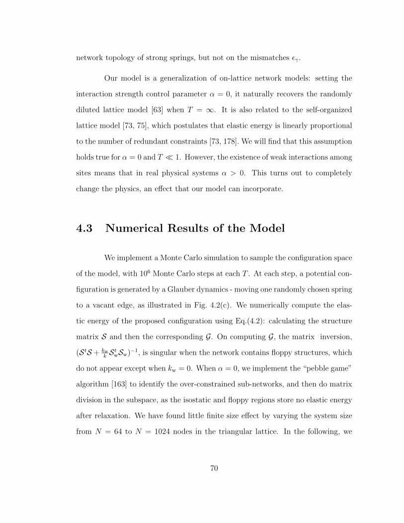
network topology of strong springs, but not on the mismatches εγ.

Our model is a generalization of on-lattice network models: setting the

interaction strength control parameter α = 0, it naturally recovers the randomly

diluted lattice model [63] when T = ∞. It is also related to the self-organized

lattice model [73, 75], which postulates that elastic energy is linearly proportional

to the number of redundant constraints [73, 178]. We will find that this assumption

holds true for α = 0 and T 1. However, the existence of weak interactions among

sites means that in real physical systems α > 0. This turns out to completely

change the physics, an effect that our model can incorporate.

4.3 Numerical Results of the Model

We implement a Monte Carlo simulation to sample the configuration space

of the model, with 106 Monte Carlo steps at each T . At each step, a potential con-

figuration is generated by a Glauber dynamics - moving one randomly chosen spring

to a vacant edge, as illustrated in Fig. 4.2(c). We numerically compute the elas-

tic energy of the proposed configuration using Eq.(4.2): calculating the structure

matrix S and then the corresponding G. On computing G, the matrix inversion,

(StS + kwkStwSw)−1, is singular when the network contains floppy structures, which

do not appear except when kw = 0. When α = 0, we implement the “pebble game”

algorithm [163] to identify the over-constrained sub-networks, and then do matrix

division in the subspace, as the isostatic and floppy regions store no elastic energy

after relaxation. We have found little finite size effect by varying the system size

from N = 64 to N = 1024 nodes in the triangular lattice. In the following, we

70

present our numerical results of networks with N = 256 nodes, averaged over 50

realizations of random mismatches if not specified.

4.3.1 Dynamics

We investigate the dynamics by computing the correlation function C(t) =

1Ns(1−Ns/3N)

(〈σ(t)|σ(0)〉 − N2s /3N), where |σ(t)〉 is the vector indicating the oc-

cupation of all edges at time t. The correlation C(t) decays from one to zero

at long time scales. We define the relaxation time τ as the time C(τ) = 1/2,

and the numerical results of τ as a function of temperature T for several different

coordination numbers are shown in the Fig. 4.4.

100

102

104

106

2

2.5

3

3.5

4

4.5

1/T

log 1

0τ

δz = −0.375

δz = −0.125

δz = +0.000

δz = +0.148

δz = +0.523

α = 0.0003

Figure 4.4: (Color online) Relaxation time τ in log-scale versus inverse temperature 1/T

for different coordination numbers δz and α = 0.0003. The solid black line indicates a

power law relation between τ and T : τ ∼ T−1/2.

71

100

105

0.6

0.7

0.8

0.9

1

1.1

1.2

T/Tg

G(z,T

)/G(z,∞

)

−1 0 1 210

−5

10−4

10−3

10−2

10−1

δz

TgorG

Tg α = 0.0

G/ ln105

Tg α = 0.0003

G/ ln105

Tg α = 0.03

G/ ln105

δz = −0.375δz = −0.125δz = +0.000δz = +0.148δz = +0.523

Figure 4.5: (Color online) Left: Shear modulus of adaptive networks at temperature T

rescaled by G at T = ∞ G(z, T )/G(z,∞), α = 0.0003. The temperature T is rescaled

by Tg. Right: Correlation between transition temperature Tg and shear modulus G in

the frozen network model [116].

We find that the implemented dynamics is not glassy. The relaxation time

increases as a power law of the temperature T−0.5, even much slower than a strong

glass that would display an Arrhenius behavior log10 τ ∝ 1/T . This result is very

surprising because the frozen elastic network model we studied earlier was glassy

(its fragility was similar to that of network liquids). Despite being dynamically

very different, these two models are almost identical as far as thermodynamics is

concerned, as we will see below. It could be that the lack of glassiness comes from

our choice of Monte-Carlo where springs can try other locations anywhere in the

system [179].

To compare the thermodynamics of these models we now need to define

an effective glass temperature Tg (even if we do not see a real glass transition).

72

We do that by using the empirical Lindemann criterion [180] according to which

an amorphous solid melts when the standard deviation 〈δR2〉1/2 of particles’ dis-

placements is greater than a fraction cL of the particle size a. The coefficient cL

must depends on the quench rate q, since this is also the case for Tg. This depen-

dence is logarithmic, because the dependence of relaxation time on temperature in

experimental glass formers is at least exponential (for typical experimental quench

rate in supercooled liquids, cL ≈ 0.15 [181]). We can estimate this standard devi-

ation via the elastic modulus if we treat the glass as a continuum 〈δR2〉 ∼ T/Ga

where G is the instantaneous shear modulus of the structure [171], we thus get

Tg ∝ Ga3/ ln(1/q). We set the lattice length a in our model to unity.

We measure the shear modulus averaging over configurations at given

temperatures, shown in the left panel of Fig. 4.5. Practically, we choose Tg =

〈G〉Tg/ ln(1/103q), where the cooling rate q is defined as the inverse of the number

of Monte Carlo steps performed at each temperature in the model. 〈•〉Tg is the

mean value at temperature Tg. The prefactor in this definition of Tg does not

affect qualitatively our conclusions, but for this pre-factor the definition of Tg

in the frozen model [116] is essentially identical to the dynamical definition used

in [116], as shown in the right panel of Fig. 4.5 by lining up G and Tg. The

specific values of Tg following that definition are shown in the inset of the bottom

panel of Fig. 4.7, they correspond to Tg = 〈G〉Tg/ ln(103) in the present model, and

Tg = 〈G〉Tg/ ln(105) in the frozen network model [116], which is simpler to simulate

and can thus be equilibrated longer.

73

100

10−10

10−8

10−6

10−4

10−2

T

E(z

,T)/N

s

100

10−6

10−5

10−4

10−3

10−2

10−1

T

C(z

,T)/N

s

100

10−5

10−4

10−3

10−2

T

nex(z

,T)

δz = −0.375δz = −0.125δz = −0.055δz = +0.000δz = +0.086δz = +0.148δz = +0.523

(a) (b) (c)

1

1.5

1

1

1

1

0.5

0.5

Figure 4.6: (Color online) Thermodynamics of the adaptive network model without

weak constraints α = 0. (a) Energy E/Ns vs. temperature; (b) specific heat C/Ns vs.

temperature; (c) excess number density of redundant constraints nex extracted using the

pebble game algorithm vs. temperature. Symbols are numerical data; solid lines are

theoretic predictions.

4.3.2 Specific heat

The specific heat data shown in Figs. 4.6 and 4.7 are our central numerical

results. The energy E = 〈H〉 is obtained using a time-average over Monte Carlo

steps, and is shown in Fig. 4.6(a). The specific heat is calculated as its derivative

c ≡ 1Ns

dE/dT , and is shown versus T for several coordination numbers when

α = 0 in Fig. 4.6(b) and α = 0.0003 in the top panel of Fig. 4.7. When α = 0,

the specific heat increases as temperature decreases for networks with δz > 0

while it meets a maximum at Ta ∼ 1 and decreases under cooling when T < Ta if

δz ≤ 0. By contrast, the specific heat increases under cooling close to the transition

temperature for all coordination numbers when α > 0. In addition, when T . α,

c→ 0.5.All these results are qualitatively identical to our previous frozen model.

To define the jump of the specific heat at the glass transition, we simply

74

100

102

104

10−4

10−3

10−2

10−1

100

T /Tg

c(z,T

)

δz = −0.375

δz = −0.125

δz = +0.000

δz = +0.148

δz = +0.523

−1 −0.5 0 0.5 1 1.5 20

0.05

0.1

0.15

0.2

0.25

0.3

0.35

0.4

0.45

0.5

δz

c(z

,Tg)

−0.5 0 0.5 1 1.5

10−4

10−3

10−2

10−1

δz

Tg

α = 0α = 0.0003α = 0.003α = 0.03

Figure 4.7: (Color online) Top: Specific heat c(z, T ) vs scaled temperature T/Tg for

networks with average coordination numbers near and away from the isostatic on both

floppy and rigid sides. The strength of the weak constraints is given by α = 0.0003.

Bottom: Specific heat at temperature Tg, c(z, Tg), vs coordination number δz for α =

0, 0.0003, 0.003, 0.03. The inset shows the transition temperature Tg for different z and

α. Symbols are numerical results, and lines are theoretical predictions: dashed lines are

for frozen network model and solid lines are for the new model derived in section IV.

measure the specific heat at our glass transition Tg defined above. This definition is

natural, since in a real glassy system, below Tg the liquid is essentially frozen in an

inherent structure, and the contribution to the specific heat from configurational

entropy (i.e. the bottom energy of inherent structures) vanishes.

Our central numerical result is shown in the bottom panel of Fig. 4.7:

c(Tg) varies nonmonotonically with the coordination number z when α > 0. When

the network of strong springs is poorly coordinated δz . 0, c(Tg) decreases as z

increases; When the strong network gets better coordinated δz & 0, c gradually

changes to increase with z; c is minimal at the proximity of the rigidity transition

zc for finite α. These numerical results are very similar to empirical observations,

75

see Point (II) in the introduction. Our data are in fact very similar to that of the

frozen model, which essentially follows the dotted lines in Fig. 4.7.

4.3.3 Number of redundant constraints R

When α = 0 and T → 0, the specific heat is simply proportional to R,

as shown in Fig. 4.6(b). This number is fixed, R = Nδz/2, in the frozen network

models. It varies in the adaptive network model and depends on the temperature.

As the Maxwell counting gives the minimal number of redundant constraints of a

network, we can define an excess number of redundant constraints

nex ≡1

Ns

(R− Nδz

2Θ(δz)

), (4.3)

where Θ(x) is the Heaviside step function. nex counts the average number of

redundant constraints, additional to the Maxwell counting. This excess number of

redundant constraints decreases monotonically to zero under cooling. When α = 0,

nex is proportional to√T in the adaptive network model at low temperature, shown

in Fig. 4.6(c).

4.4 Theory of Thermodynamics

As illustrated in Fig. 4.8, in the frozen elastic model we found that as

α→ 0, c converges to a constant if z < zc, whereas it behaves as z− zc for z > zc.

As α is increased, the discontinuous behavior becomes smooth and looks similar to

experimental data. We seek to derive these same features in the adaptive network

76

∆cp(z)

0 δz

∼ 1

Figure 4.8: (Color online) Theoretical predictions for the jump of specific heat. For

vanishingly weak springs α→ 0, it is predicted that the jump is essentially constant for

z < zc and then drops to zero a zc. For larger z, it behaves as z − zc. As α grows this

sharp curve becomes smooth, but a minimum is still present near z = zc.

models.

4.4.1 Partition function

For simplicity, we consider the annealed free energy Fann = −T lnZ. It

is exact in the random energy model [136] above the ideal glass transition [182]

and we find it to be a good approximation of F in our models [116]. The over-line

implies an average over disorder ε,

Z =∑σ

∑perm[γ]

exp[−H(Γ)/T ] (4.4)

77

where a given configuration Γ is characterized by σ indicating which edges are

occupied on the triangular lattice, and perm[γ] labels the possible permutations of

springs’ rest lengths.

We first average over the quenched randomnesses. Using the linear ap-

proximation Eq.(4.2) and the Gaussian distribution ρ(εγ) = 1√2πε2

e−ε2γ/2ε

2,

Z =∑σ

(Nz

2

)! exp

[−1

2tr ln

(I +G(σ)T

)](4.5)

The factorial comes from Ns! =∑

perm[γ] 1 as G is independent of the permutation.

I is a 3N×3N identity matrix; each component corresponds to an edge on the lat-

tice. To compute the trace in the exponent, we first make the approximation that

the weak springs are weak and numerous StwSw ≈ zwdINd×Nd, which corresponds

to the highly connected limit zw → ∞ and finite α. We can then decompose the

coupling matrix G ≈ P − S(StS + αI)−1St as [116]:

G(σ) =∑p(σ)

|ψp〉〈ψp|+∑

ω(σ)>0

α

ω2 + α|ψω〉〈ψω| (4.6)

where p labels the vectors |ψp〉 satisfying St|ψp〉 = 0 (i.e. a basis for the kernel

of St), and where the |ψω〉 satisfy SSt|ψω〉 = ω2|ψω〉. The number of redundant

directions is∑

p 1 = Ns − (Nd− F ) ≡ R. Note that trP = Ns, Nd− F gives the

number of frequencies ω, and F counts the number of floppy modes. The modes

|ψp〉, |ψω〉, R, and ω depend on occupation σ. As the |ψ〉’s are orthonormal, the

78

trace in Eq.(4.5) gives

Z =

(Nz

2

)!∑

nr,D(ω)

exp

[Ns

(s(nr, D(ω))− nr

2ln(1 +

1

T)

−1− nr2

∫dωD(ω) ln(1 +

1

T

α

ω2 + α)

)], (4.7)

where s(nr, D(ω)) ≡ 1Ns

ln∑σ 1R,D(ω) is configurational entropy density with

given number of redundant constraints nr ≡ R/Ns and density of vibrational

modes, D(ω), satisfies (1− nr)∫

dωD(ω) ≡ limN→∞1Ns

∑ω>0.

4.4.2 No weak interactions

(b) z > zc(a) z < zc

Figure 4.9: (Color online) (a) z < zc, localized redundant constraints (red) in a floppy

sea (blue); (b) z > zc localized floppy modes (blue) in a rigid sea (red and green).

Neglecting the weak constraints α = 0, the last term in the exponential

vanishes and the summation over states with given density of states can be ab-

sorbed into the entropy, which then depends only on the number of redundant

79

constraints.

Z =

(Nz

2

)!∑nr

eNs[s(nr)−nr2

ln(1+ 1T

)] (4.8)

We propose an ideal-gas picture of “defects” to find an approximation

form of the entropy s(nr). When the coordination number is very small z < zc

and the network is mostly floppy, redundant constraints are defects localized in

rigid islands. Similarly, when the coordination number is very large z > zc with

most regions of the network rigid, there are localized floppy modes in regions where

there are negative fluctuations of coordination number, which we again described

as defects, see illustration in Fig. 4.9. The number of such floppy modes is equal

to the number of additional over-constrained in the rigid cluster. The entropy

gains from having these defects. Assuming that such defects are independent, we

approximate the entropy by that of an ideal gas:

s(nex) ≈ s(0)− nex lnnex

en0(z)(4.9)

where nex is the excess number of redundant constraints defined in Eq.(4.3) and is

thus counting the number of defects. s(0) is the entropy density of the states with a

minimal number of redundant constraints (i.e. they satisfy the Maxwell counting);

and n0(z) is the excess number of redundant constraints at T =∞. Both s(0) and

n0 depend only on z and the lattice structure. This form of Eq.(4.9) fails when the

assumption of independent “defects” breaks down, as must occur near the rigidity

transition. However, our numerical results indicate that this approximation is very

accurate, we see deviations only for |δz| . 0.1.

We numerically test the formula Eq.(4.9) for a triangular lattice. The

80

0 2 4 6 810

−4

10−3

10−2

10−1

100

β

nex(z,β

)/nex(z,0

)

10−1

100

101

10−2

10−1

100

101

102

β

(∆nr(z,β

))2/nex(z,β

)

δz = −0.395δz = −0.113δz = −0.055δz = −0.004δz = +0.068δz = +0.131δz = +0.506

∼ e−β∼ β2

Figure 4.10: (Color online) Left: Excess number density of redundant constraints

nex(z, β). Right: Fluctuation of the number density of redundant constraints (∆nr)2.

The solid black lines show the predictions from the approximate entropy Eq.(4.9).

configurations with R redundant constraints are weighted by e−βR for different

values of the parameter β. From Eq.(4.9), the mean and variance of the excess

number density of redundant constraints, nex, satisfy the following formulas:

β ≡ ∂s

∂nex

⇒ nex(z, β) = n0(z)e−β (4.10a)

∆n2ex(z, β) = −β2 ∂

∂βnex(z, β) = β2nex(z, β) (4.10b)

Our numerical results coincide with Eqs.(4.10a) and (4.10b) remarkably well, with

minor deviations for |δz| . 0.1, as shown in Fig. 4.10.

Applying Eq.(4.9), we derive the thermodynamics of our model when α =

81

0. Solving the saddle point of Eq.(4.8), we obtain the average energy density:

1

Ns

E(z, T ) =r0 + nex(z, T )

2

T

1 + T(4.11a)

the specific heat:

1

Ns

C(z, T ) =r0 + 3

2nex(z, T )

2

1

(1 + T )2(4.11b)

and the excess number density of redundant constraints:

nex(z, T ) = n0(z)

(1 +

1

T

)−1/2

(4.11c)

where r0 ≡ δzz

Θ(δz).

As n0(z) is expected to be an analytic function of z, Eqs.(4.11) indicate

that c converges to the one found in frozen network model in the limit T → 0:

c = 0 when δz < 0 and c = δz/2z when δz > 0 - the dashed yellow line in Fig. 4.8.

This is our first central result, which shows that our previous results hold even

when the network is adaptive.

Eqs.(4.11) predict the energy, specific heat, and the number density of

redundant constraints at an arbitrary temperature without any fitting parameter.

The solid lines, shown in Fig. 4.6(a) and (b), are predictions of Eqs.(4.11a) and

(4.11b), respectively, with nex as the numerical input. They are closely consistent

with the data points, which confirms the annealed free energy approximation when

α = 0. A T 1/2 power-law with numerical prefactor n0(z) = nex(z,∞) predicted by

Eq.(4.11c) coincides well with data points in Fig. 4.6(c).

Extending to finite glass transition Tg at α = 0, we find a correction

82

vanishing as√δz in addition to c ≈ δz/2z, assuming Tg ∼ G ∼ δz for z > zc. But

this correction is quantitatively unimportant as n0 ≤ 0.03 and does not change

qualitatively the linear growth of the specific heat when δz > 0, as illustrated by

the solid orange line in Fig. 4.8.

Our theoretic prediction that nex → 0 when T → 0 validates the assump-

tions of [73, 75, 178] that the energy of redundant bonds is proportional to their

number, and that this number is R0 at T = 0.

4.4.3 General case

In the thermodynamic limit, Ns →∞, we take the saddle point of Eq.(4.7),

2∂s

∂nr= ln

(1 +

1

T

)−∫

dωD(ω) ln

(1 +

1

T

α

ω2 + α

)(4.12a)

and

2δs

δD(ω)= (1− nr) ln

(1 +

1

T

α

ω2 + α

)(4.12b)

and solve for energy,

1

Ns

E(z, T, α) =nr(T )

2

T

1 + T

+1− nr(T )

2

∫dωD(ω, T )

αT

α + (ω2 + α)T(4.13)

The specific heat predictions from differentiating Eq.(4.13) with numerical inputs

nr(z, T, α) and Dz,T,α(ω) are plotted as solid lines in Fig. 4.7. (See Appendix

Secs. C.2, C.3, and C.4 for the temperature dependence of D(ω).) Notice that

replacing nr(T ) by δz/z and D(ω, T ) by its low-temperature limit D(ω) studied

83

in [78, 116, 130], Eq.(4.13) recovers exactly the one obtained in the frozen network

model, whose predictions are plotted as dashed lines in Fig. 4.7. The dashed

lines converge to the solid lines despite differences at high temperatures for weakly

coordinated networks.

In the limit α→ 0 and T α, Eq.(4.13) converges to E/Ns = T/2, which

indicates a constant specific heat c = 0.5 when δz < 0 independent of the models.

This is shown by the solid orange line and the dashed yellow line in Fig. 4.8, and

is our second key theoretical result showing the robustness of our conclusions for

adaptive networks.

4.5 Conclusions

In this work, we have studied the correlation between the elasticity of

inherent structures and the thermodynamics in covalent glass-forming liquids using

adaptive network models. We found numerically and explained theoretically why

these models have a thermodynamic behavior similar to frozen network models

[116] which captures nicely experimental facts.

The main prediction conclusion of [116] is thus robust: as the coordination

number approaches zc from above, elastic frustration vanishes. This leads both to

an abundance of soft elastic modes, as well as a diminution of the number of

directions in phase space that cost energy, which is directly proportional to the

jump of specific heat. Below the rigidity transition, the elasticity of strong force

network vanishes, thus the energy landscape is governed by the weak Van der Waals

interactions. At these energy scale, all directions in contact space have a cost, and

84

thus the specific heat increases. Thus thermodynamic properties are governed by

a critical point at δz = 0, α = 0 where the jump of specific heat is zero. This

prediction focuses on the configurational part of the jump of specific heat, since we

considered only the energy minima in the metastable states. In Appendix Sec. C.5,

we argue that the vibrational contribution to this jump is so small in our models.

Thus the main prediction of the specific heat still holds, even when including the

vibrational part.

Beyond network glasses, our main result potentially explains the correla-

tion between elasticity and the key aspects of the energy landscape in molecular

glasses [4, 35, 77]. Indeed according to our work we expect glasses with a strong

Boson peak to display less elastic frustration, so that they have a limited number

of directions in phase space costing energy, see discussion in [116].

85

Chapter 5

A Model for the Erosion Onset of

a Granular Bed Sheared by a

Viscous Fluid

We study theoretically the erosion threshold of a granular bed forced by

a viscous fluid. We first introduce a novel model of interacting particles driven on

a rough substrate. It predicts a continuous transition at some threshold forcing

θc, beyond which the particle current grows linearly J ∼ θ − θc. The stationary

state is reached after a transient time tconv which diverges near the transition as

tconv ∼ |θ − θc|−z with z ≈ 2.5. Both features agree with experiments. The

model also makes quantitative testable predictions for the drainage pattern: the

distribution P (σ) of local current is found to be extremely broad with P (σ) ∼ J/σ,

spatial correlations for the current are negligible in the direction transverse to

forcing, but long-range parallel to it. We explain some of these features using

86

a scaling argument and a mean-field approximation that builds an analogy with

q-models. We discuss the relationship between our erosion model and models for

the plastic depinning transition of vortex lattices in dirty superconductors, where

our results may also apply.

5.1 Introduction

Erosion shapes Earth’s landscape, and occurs when a fluid exerts a suf-

ficient shear stress on a sedimented layer. It is controlled by the dimensionless

Shields number θ ≡ Σ/(ρp − ρ)gd, where d and ρp are the particle diameter and

density, and ρ and Σ are the fluid density and the shear stress. Sustained sediment

transport can take place above some critical value θc [84, 85, 87], in the vicinity of

which motion is localized on a thin layer of order of the particle size, while deeper

particles are static or very slowly creeping [82, 86, 88]. This situation is relevant

in gravel rivers, where erosion occurs until the fluid stress approaches threshold

[7]. In that case, predicting the flux J of particles as a function of θ is difficult,

both for turbulent and laminar flows [6, 86, 92, 183]. We focus on the latter, where

experiments show that: (i) in a stationary state, J ∝ (θ− θc)β with β ≈ 1 [81, 86,

88, 89], although other exponents are sometimes reported [87], (ii) transient effects

occur on a time scale that appears to diverge as θ → θc [86, 88] and (iii) as θ → θc

the density m of moving particles vanishes, but not their speed [86, 89, 90].

Two distinct views have been proposed to describe erosion near threshold.

For Bagnold [6] and followers [92], hydrodynamics is key: moving particles carry

a fraction of the stress proportional to their density m, such that the bed of

87

static particles effectively remains at the critical Shields number. This argument

implies m ∼ θ− θc, in agreement with (i,iii). However, it treats the hydrodynamic

effect of a moving particle on the static bed in an average (mean-field) way, and

its application when moving particles are far apart (i.e. m 1) may thus not

be warranted. By contrast, erosion/deposition models [86] emphasize the slow

“armoring” or “leveling” of the particle bed. One assumes that a θ-dependent

fraction of initially mobile particles evolve over a frozen static background, which

contain holes. In this view, θc occurs when the number of holes matches the number

of initially moving particles. This phenomenological model also leads to m ∼ θ−θc

and captures (i,ii,iii) qualitatively well. However, the implicit assumption that the

moving particles visit the static bed entirely (thus filling up all holes) is highly non-

trivial. Indeed, due to the disorder of the static bed one expects mobile particles to

follow favored paths and to eventually flow in a few channels, thus exploring a tiny

region of space. Such disorder-induced coarsening dynamics occurs for example in

river networks models [95], as well as plastic-depinning models of vortex lattices

in dirty superconductors [97, 98] which also display a transition, but with β ≈ 1.5,

at odd with (i).

To decide which physical process (hydrodynamic interactions or armoring)

governs the erosion threshold, new theoretical predictions must be made and put to

experimental test. In this letter, we achieve the first step of this goal while resolving

the apparent contradictions of deposition models. Specifically, we introduce a

model of interacting particles forced along one direction on a disordered substrate.

Particle interactions based on mechanical considerations are incorporated. Such

model recovers (i,ii,iii) with β = 1 and an equilibration time tconv ∼ |θ − θc|−2.5,

which agrees quantitatively with experiments [88]. Our most striking predictions

88

concerns the spatial organization of the flux near threshold, which emerges from

the interplay between disorder and particle interaction: (a) the distribution of local

flux σ is extremely broad, and follows P (σ) ∼ 1/σ and (b) spatial correlations of

flux are short-range and very small in the lateral direction, but are power-law in

the mean flow direction. We derive β = 1 and explain why P (σ) is broad using

a mean-field description of our model, leading to an analogy with q-models [184,

185] used to study force propagation in grains.

5.2 Erosion Model

We consider a density n of particles on a frozen background. n should be

chosen to be of order one, but its exact value does not affect our conclusions. The

background is modeled via a square lattice, whose diagonal indicates the direction

of forcing, referred to as “downhill”. The lattice is bi-periodic, of dimension L×W ,

where L is the length in downhill direction and W the transverse width. Each node

i of the lattice is ascribed a height hi ∈ [0, 1], chosen randomly with a uniform

distribution. Lattice bonds i → j are directed in the downhill direction, and

characterized by an inclination θi→j = hi − hj. We denote by θ the amplitude of

the forcing. For an isolated particle on site i, motion will occur along the steepest

of the two outlets (downhill bonds) [96], if it satisfies θ+ θi→j > 0. Otherwise, the

particle is trapped.

However, if particles are adjacent, interaction takes place. First, particles

cannot overlap, so they will only move toward unoccupied sites. Moreover, particles

can push particles below them, potentially un-trapping these or affecting their

89

direction of motion. To model these effects, we introduce scalar forces fi→j on

each outlet of occupied sites, which satisfy:

fi→j = max(fj′→i + θi→j + θ, 0) (5.1)

where fj′→i is the force on the input bond j′ → i along the same direction as i→ j,

as depicted in Fig. 5.1. Eq.(5.1) captures that forces are positive for repulsive

particles, and that particle i exerts a larger force on toward site j if the bond

inclination θi→j is large, or if other particles above i are pushing it in that direction.

From our analysis below, we expect that the details of the interactions (contacts,

lubrication forces, etc...) are not relevant, as long as the direction of motion of one

particle can depend on the presence of particles above it- an ingredient not present

in [97, 98].

We update the position of the particles as follows, see Fig. 5.1 for illustra-

tion. We first compute all the forces in the system. Next we consider one row of W

sites, and consider the motion of its particles. Priority is set by considering first

outlets with the largest fi→j and unoccupied downhill site j. Once all possible

moves ( fi→j > 0, j empty) have been made, forces are computed again in the

system, and the next uphill row of particles is updated. When the L rows forming

the periodic system have all been updated, time increases by one.

For given parameters θ, n we prepare the system via two protocols. In

the “quenched” protocol, one considers a given frozen background, and launch

the numerics with a large θ and randomly placed particles - parameters are such

that the system is well within the flowing phase. Next, θ is lowered slowly so

that stationarity is always achieved. We also consider the “Equilibrated” proto-

90

t t + 1

1

2

3

4

5

6

7

8

9

10

1 2 3

A A

B B

C C

j ′

i

j

Figure 5.1: Illustration of the model. Small circles indicate lattice sites, particles are

represented by discs in yellow, or green if motion occurred between t (left) and t + 1

(right). The black arrow is in the downhill direction. Solid lines indicate outlet with

positive forces. If a particle has two outlets with positive forces, the larger (smaller) one

is colored in red (blue).

col: for any θ, particles initial positions are random. Dynamical properties are

measured after the memory of the random initial condition is lost. We find that

using different protocols does not change critical exponents, but that the quenched

protocol appears to converge more slowly with system size. Below we present most

of our results obtained from the “equilibrated” protocol with W = 4√L [98], and

n = 0.25 unless specified.

91

10−3

10−2

10−1

10−2

10−1

θ − θc

J(θ

)

10−3

10−2

10−1

10−2

10−1

θ − θc

J(θ

)

−0.1 −0.05 0 0.05 0.1 0.15 0.20

0.2

0.4

0.6

0.8

1

θ − θc

ρs(θ

)

−0.5 0 0.5 10

0.2

0.4

0.6

0.8

1

(θ − θc)L1/ν

ρs(θ

)

L = 16

L = 32

L = 64

L = 128

L = 256

(b)

(c) (d)

(a)

Figure 5.2: Average current J versus θ − θc in log-log scale for the (a) “equilibrated”

and (b) “quenched” protocols, for which θc = 0.164 ± 0.002 and θc = 0.172 ± 0.002

respectively- a difference plausibly due to finite size effects. The black solid lines with

slope one indicate the linear relation J ∝ θ−θc. (c) Density of conducting sites ρs versus

θ − θc for the “equilibrated” protocol. (d) ρs curves collapsed by rescaling θ − θc with

L1/ν , where ν = 3.0± 0.2.

5.3 Numerical Results on Dynamics of the Model

Once the steady state is reached, we measure the average current of parti-

cles J and the number density of sites carrying a finite current ρs. Measurements of

92

both quantities indicate a sharp dynamical transition at some θc below which J = 0

and ρs = 0 as L→∞, see Fig. 5.1. θc can be accurately extracted by considering

the crossing point of the curves ρs(θ) as L is varied, yielding θc = 0.164± 0.002 for

the equilibrated protocol. In the limit L→∞ our data extrapolates to:

J(θ) ∼ θ − θc for θ > θc (5.2)

ρs(θ) = Θ(θ − θc), (5.3)

where Θ is the Heaviside function. Eq.(5.2) corresponds to β = 1, whereas Eq.(5.3)

indicates that all sites are visited by particles in the flowing phase. Introducing the

exponent ρs(θ) ∼ (θ − θc)γ, this corresponds to γ = 0. The collapse of Fig. 5.2(d)

shows how convergence to Eq.(5.3) takes place as L→∞, from which a finite size

scaling length ξ ∼ (θ − θc)−ν with ν ≈ 3 can be extracted.

Criticality is also observed in the transient time tconv needed for the current

to reach its stationary value. Fig. 5.3 reports that tconv ∼ |θ − θc|−z with z ≈ 2.5

on both sides of the transition, which captures accurately the experiments of [88]

and the numerics of [91].

The spatial organization of the current in steady state can be studied by

considering the time-averaged local current σi on site i, or the time-averaged outlet

current σi→j. The spatial average of each quantity is J . Fig. 5.4 shows an example

of drainage pattern, i.e. one realization of the map of the σi→j.

To quantify such patterns, we compute in Fig. 5.5(a) the distribution P (σ)

93

−0.2 −0.1 0 0.1 0.2 0.310

0

101

102

103

104

θ − θc

t conv

L = 16L = 32L = 64L = 128L = 256

tconv∼ |θ − θc|−2.5

10−2

10−1

10010

0

101

102

103

104

θ − θc

t conv(s)

Data from Ref.[6]

y = x−2.5/10

Figure 5.3: Left: Transient time tconv v.s. θ. For a given realization, tconv is defined as

the smallest time for which J(t)−J ≤√V ar(J) where V ar(J) = limT→∞

1T

∑Tt=1(J(t)−

J)2. The gray dashed lines correspond to tconv ∼ |θ − θc|−2.5. Right: The obtained

exponent fits well the observations of [88].

of the local current σi for various mean current J . We observed that:

P (σ) = Jσ−τf(σ) (5.4)

where τ ≈ 1 and f is a cut-off function, expected since in our model σi < 1.

Eq.(5.4) indicates that P (σ) is remarkably broad. In fact, the divergence at small

σ is so pronounced that a cut-off σmin must be present in Eq.(5.4) to guarantee

a proper normalization of the distribution P (σ), although we cannot detect it

numerically.

Next, we compute the spatial correlation of the local current in the trans-

94

θ−

cθ+

c

Figure 5.4: Examples of drainage pattern just below θc (Left) and above (Right). The

black arrow shows the downhill direction. The thickness of the lines represents σi→j in

logarithmic scale. A few examples showing splitting events are magnified on the left.

Here W = 45 and L = 128, and J > 0 even below θc due to finite size effects.

verse direction CT (x), defined as:

CT (x) = (〈σiσi+x〉 − J2)/(〈σ2i 〉 − J2) (5.5)

where the site i and i + x are on the same row, but at a distance x of each

other. Here the brackets denote the spatial average, whereas the overline indicates

averaging over the quenched randomness (the hi’s). Fig. 5.6(a) shows that no

transverse correlations exist for distances larger that one site. However, long-range,

power-law correlations are observed in the longitudinal direction, as can be seen by

defining a longitudinal correlation function CL(y), where y is the vertical distance

between two sites belonging to the same column. We find that CL(y) ∼ 1/√y at

95

10−2

10−1

100

10−1

100

101

102

σ

P(σ

)/J

J = 0.204

J = 0.152

J = 0.136

J = 0.118

J = 0.096

10−3

10−2

10−1

100

10−2

100

102

104

σ

P(σ

)/J

J = 0.100J = 0.030J = 0.010J = 0.003J = 0.001

x−3/2exp(−10x4)

(a) (b)

1.5

1.0

1.0

1.0

Figure 5.5: Distribution of the site current P (σ) in steady state for given average

currents J of (a) the erosion model (L = 256, W = 64) and (b) our mean-field model

(W = 1600).

θc, but that CL(y) decays somewhat faster deeper in the flowing phase, as shown

in Fig. 5.6(b).

100

101

102

10−2

10−1

100

y

CL(y

)

0 5 10 15 20 25 30 35−0.2

0

0.2

0.4

0.6

0.8

1

1.2

x

CT(x

)

L = 16

L = 32

L = 64

L = 128

L = 256

(a) (b)

1.0

1.0

0.50

0.70

Figure 5.6: (a) Transverse current correlations CT at θc and (b) longitudinal current

correlation CL at θc and at θ − θc = 0.25 for L = 256 (dashed line).

96

5.4 An Argument on the Scaling Relation

We now derive a relationship between the exponents β characterizing J

and γ characterizing ρs. It holds true for both protocols, but is presented here in

the “quenched” case. Near threshold, at any instant of time the density of moving

particles is J n < 1, thus most of the particles are trapped and will move only

when a mobile particle passes by. As θ is decreased by some δθ, a finite density

of new traps δm ∼ δθ is created. If these traps appear on the region of size ρs

where mobile particles flow, they will reduce the fraction of mobile particle by

δJ = ρsδm ∼ ρsδθ, which implies:

β = γ + 1 (5.6)

Eq.(5.6) shows that the result β = 1 is a direct consequence of the fact that in our

model, all sites are explored by mobile particles for θ > θc, a result which is not

obvious. In the dirty superconductor models of [98, 186], this is not the case and

for the “equilibrated” protocol β > 1 was found. We argue that this difference

comes from the dynamical rules chosen in [98, 186], according to which “rivers”

forming the drainage pattern never split: their current grows in amplitude in the

downhill direction, until it reaches unity. In these models the drainage pattern thus

consists of rivers of unit current, avoiding each other, and separated by a typical

distance of order 1/J . Our model behaves completely differently because rivers

can split, as emphasized in Fig. 5.4. This comes about because the direction taken

by a particle can depend on the presence of a particle right above it, as illustrated

in case A of Fig. 5.1. This effect is expected to occur in the erosion problem due

to hydrodynamic interactions or direct contact between particles, and may also be

97

relevant for superconductors.

5.5 Mean-field Model on the Distribution of Lo-

cal Currents

We now seek to quantify the effect of splitting. Its relevance is not obvious

a priori, as splitting stems from particle interactions, and may thus become less

important as the fraction of moving particles vanishes as J → 0. To model this

effect we consider that the current σi on a site i is decomposed in its two outlets

as σi = qσi + (1− q)σi, where q is a random variable of distribution η(q). If there

were no splitting then η(q) = 12δ(q) + 1

2δ(1 − q). Here instead, we assume that

η(q) = 12δ(q−J)+1

2δ(1−J−q). This choice captures that the probability of splitting

is increased if more moving particles are present, and can occur for example if two

particles flow behind each other, as exemplified in case A of Fig. 5.1. Next, we

make the mean field assumption that two adjacent sites i and j on the same row are

uncorrelated, P (σi, σj) = P (σi)P (σj). We then obtain the self-consistent equation

that P (σ) must be equal to:

∫dq1dq2dσ1dσ2η(q1)η(q2)P (σ1)P (σ2)δ(q1σ1 + q2σ2 − q) (5.7)

This mean-field model belongs to the class of q-models introduced to study force

propagation [184, 185]. It is easy to simulate, and some aspects of the solution can

be computed. Numerical results are shown in Fig. 5.5(b). The result obtained for

P (σ) is very similar to Eq.(5.4) that describes our erosion model: P (σ) is found

98

to be power-law distributed (although τ = 3/2 instead of τ = 1) where with an

upper cutoff at σmax ∼ 1, and P (σ) ∝ J .

These results are of interest, as they explain why P (σ) is very broad, and

is not dominated by sites displaying no current at all (which would correspond to

a delta function at zero) even as J → 0, thus confirming that γ = 0. They can

be explained by taking the Laplace transform P of Eq.(5.7). One then obtains a

non-linear differential equation for P , from which it can be argued generically that

τ = 3/2 [185]. We have performed a Taylor expansion of P around zero, which

leads to relationship between the different moments of the distribution P (σ). From

it, we can show that P (σ) ∝ J and σmax ∼ 1. We also find that the cut-off of the

divergence of P (σ) at small argument follows σmin ∼ J1/(τ−1).

5.6 Potential Experimental Tests

We have introduced a novel model for over-damped interacting particles

driven on a disordered substrate. It predicts a dynamical phase transition at some

threshold forcing θc, and makes quantitative predictions for various quantities in-

cluding the particle current and the drainage pattern, testable by tracking parti-

cles on the surface [86]. Our model includes the possibility that channels carrying

most of the flow split, which may also be well-suited to describe plastic depinning

phenomena including the pinning of vortices in dirty superconductors [97, 187]

or driven colloidal systems [188, 189], which have never been received a proper

analytical treatment 2.

2 In plastic depinning an exponent β ≥ 1.5 is often reported, larger than our predicted β = 1.However we observe that large systems are required to measure β accurately, and that in smaller

99

Note that our model assumes that particles are over-damped, and that

their inertia is negligible. We expect inertia to lead to hysteresis and make the

transition first order, as observed on inertial granular flows down an inclined plane

[190], although this effect may be small in practice [191]. We did not consider non-

laminar flows, nor temperature (that can be relevant for colloids). Both effects

should smooth the transition, and lead to creep even below θc.

systems β can appear significantly larger.

100

Chapter 6

Dynamics and Correlations

among Soft Excitations in

Marginally Stable Glasses

Marginal stability is the notion that stability is achieved, but only barely

so. This property constrains the ensemble of configurations explored at low tem-

perature in a variety of systems, including spin, electron and structural glasses.

A key feature of marginal states is a (saturated) pseudo-gap in the distribution

of soft excitations. We examine how such pseudo-gaps appear dynamically by

studying the Sherrington-Kirkpatrick (SK) spin glass. After revisiting and correct-

ing the multi-spin-flip criterion for local stability, we show that stationarity along

the hysteresis loop requires soft spins to be frustrated among each other, with a

correlation diverging as C(λ) ∼ 1/λ, where λ is the stability of the more stable

spin. We explain how this arises spontaneously in a marginal system and develop

101

an analogy between the spin dynamics in the SK model and random walks in two

dimensions. We discuss analogous frustrations among soft excitations in short

range glasses and how to detect them experimentally. We also show how these

findings apply to hard sphere packings.

6.1 Introduction

In glassy materials with sufficiently long-range interactions, stability at

low temperature imposes an upper bound on the density of soft excitations [101].

In electron glasses [102, 103, 192–195] stability towards hops of individual localized

electrons requires that the density of states vanishes at the Fermi level, exhibiting a

so-called Coulomb gap. Likewise, in mean-field spin glasses [11, 104–107, 196–198]

stability towards flipping several “soft” spins implies that the distribution of local

fields vanishes at least linearly. In hard sphere packings the distribution of forces

between particles in contact must vanish analogously, preventing that collective

motions of particles lead to denser packings [56, 108, 109]. Often, these stability

bounds appear to be saturated [104, 109–111, 194, 198]. Such marginal stability

can be proven for dynamical, out-of-equilibrium situations under slow driving at

zero temperature [101] if the effective interactions do not decay with distance. This

situation occurs in the Sherrington-Kirkpatrick (SK) model (see Eq. (6.1) below),

but also in finite-dimensional hard sphere glasses, where elasticity induces non-

decaying interactions [128]. Marginality is also found for the ground state or for

slow thermal quenches by replica calculations for spin glass [105, 199] and hard

sphere systems [115, 200], assuming infinite dimension.

102

The presence of pseudo-gaps strongly affects the physical properties of

these glasses. The Coulomb gap alters transport properties in disordered insula-

tors [102, 103], while its cousin in spin glasses suppresses the specific heat and

susceptibility. It was recently proposed that the singular rheological properties of

dense granular and suspension flows near jamming are controlled by the pseudo-

gap exponents in these systems [201]. More generally, an argument of Ref. [101]

shows that a pseudo-gap implies avalanche-type response to a slow external driving

force, so-called crackling [202], for a range of applied forcing. Such behavior is

indeed observed in these systems [104, 194, 203] and in the plasticity of crystals

[204], and contrasts with depinning or random field Ising models where crackling

occurs only at one specific value of forcing [9, 205, 206]. Despite the central role

of pseudo-gaps, it has not been understood how they emerge dynamically, even

though some important elements of the athermal dynamics of the SK spin glass

have been pointed out in earlier works [106, 197].

In this Letter we identify a crucial ingredient that was neglected in previ-

ous dynamical approaches, and also in considerations of multi-spin stability: Soft

spins are strongly frustrated among each other, a correlation that becomes nearly

maximal for spins in the weakest fields. We expect analogous correlations in

short range spin glasses, which can be probed experimentally. These correlations

require revisiting earlier multi-spin stability arguments that assumed opposite cor-

relations. We then argue, assuming stationarity along the hysteresis loop, that the

correlation C(λ) between the softest spins and spins in local fields of magnitude λ

must follow C(λ) ∼ 1/λγ, with γ = 1. Using this in a Fokker-Planck description

of the dynamics we predict the statistics of the number of times a given spin flips

in an avalanche.

103

6.2 Dynamics of Sherrington-Kirkpatrick Model

We consider the SK model with N Ising spins (si = ±1) in an external

field h:

H = −1

2

∑i 6=j

Jijsisj − hN∑i=1

si. (6.1)

All spins are coupled to each other by a symmetric matrix Jij, whose elements

are i.i.d. Gaussian random variables with zero mean and variance 1/N . The total

magnetization is M ≡∑

i si. We define the local field hi and the local stability λi

of spin i by

hi ≡ −∂H∂si

=∑j 6=i

Jijsj + h, λi = hisi. (6.2)

The spin si is called stable when it aligns with the local field, i.e. if λi > 0, and

unstable otherwise. The energy to flip the spin si → −si (and hence λi → −λi) is:

∆H1(i) ≡ H(−si)−H = 2si(∑j 6=i

Jijsj + h) = 2λi. (6.3)

As in Ref. [104], we consider the hysteresis loop at zero temperature ob-

tained by quasi-statically increasing the field, as shown in Fig. 6.1(a). When a spin

turns unstable, we apply a greedy Glauber dynamics that relaxes the system in

an avalanche-like process towards a new one-spin-flip stable state by sequentially

flipping the most unstable spin. Such hysteretic field ramping has also been used

to find approximate ground states [207, 208]. Those states empirically exhibit a

pseudo-gap in the distribution of the λi [104, 197, 198],

ρ(λ) = Aλθ +O(N−θ/(1+θ)), (6.4)

104

with θ = 1 for λ 1, as shown in Fig. 6.1(b), but with a slope A significantly

larger than in equilibrium [105, 106, 209]. The avalanche size is power-law dis-

tributed [104]:

D(n) = n−τd(n/Nσ)/Ξ(N), (6.5)

where n is the number of flips in an avalanche. The scaling function d(x) vanishes

for x 1. Nσ is the finite size cutoff, and Ξ(N) is a size dependent normalization if

τ ≤ 1. Numerical studies of the dynamics of the SK model indicate that τ = σ = 1

and Ξ = lnN [104, 198], as shown by the finite size collapse in Fig. 6.1(c). While

one can argue that θ = 1 along the hysteresis curve [101], the exponents τ and

σ have not been derived theoretically for the dynamics (unlike for “equilibrium

avalanches”, for which τ = 1 has been obtained analytically [11, 107]).

Below we present a theoretical analysis of the dynamics. We assume

that the average number of times a spin flips along the hysteresis loop diverges

with N for any finite interval of applied field [h, h + ∆h] if h = O(1). This as-

sures that a stationary regime is reached rapidly. (For τ = 1 this condition simply

reads σ + 1/(1 + θ) > 1) 1. We further rely on θ < ∞. This implies a diverg-

ing number of avalanches in the hysteresis loop, each contributing a subextensive

amount of dissipation 1. The latter rules out avalanches running into strongly

unstable configurations, with an extensive number of spins with negative stability

|λ| = O(1). Thus, the lowest local stability encountered in an avalanche, λ0, must

satisfy λ0 → 0 as N →∞, as we confirm numerically in Fig. 6.2(a).

1The typical external field increment triggering an avalanche is hmin ∼ λmin ∼ N−1/(1+θ), sothere are Nav ∼ 1/hmin ∼ N1/(1+θ) avalanches in a finite range of external field dh [101]. Eachavalanche contains on average Nflip ∼

∫nD(n)dn ∼ N (2−τ)σ flip events. The total number of flip

events along the hysteresis curve is NavNflip ∼ N (2−τ)σ+1/(1+θ), which we assume to be N .1.

105

−4 −2 0 2 4−1

−0.5

0

0.5

1

h

M(h

)/N

0 0.5 1 1.5 2 2.5 30

0.1

0.2

0.3

0.4

0.5

0.6

λ

ρ(λ

)

10−3

10−2

10−1

100

101

10−4

10−3

10−2

10−1

100

101

n lnN/N

D(n

)nln

N

0 0.5 1 1.5 2 2.5 3−4

−3

−2

−1

0

1

2

λ

NC(λ

)[λ+

c(N

)]N = 0100N = 0150N = 0200N = 0300N = 0500N = 0700N = 1000N = 1500N = 2000N = 3000N = 5000N = 7000

(c)

(a) (b)

(d)

Figure 6.1: (a) Hysteresis loop: MagnetizationM under a periodic quasi-static driving of

the external field h. Inset: magnified segment of the hysteresis loop of a finite size system.

(b) Distribution of local stabilities, ρ(λ), in locally stable states along the hysteresis loops

for different system sizes N . (c) Finite size scaling of the avalanche size distribution

D(n) confirms τ = σ = 1 up to logarithmic corrections. (d) Correlation C(λ) between

the least stable spin and spins of stability λ in locally stable states along the hysteresis

loop. The data for different system sizes collapses, implying C(λ 1) ∼ 1/λ in the

thermodynamic limit.

6.3 Multi-spin Stability Criterion

A static bound for the pseudogap exponent θ is obtained by considering

two of the softest spins i, j (with stabilities λmin ∼ 1/N1/(1+θ)) [101, 113, 114].

106

100

101

102

103

104

105

100

101

102

103

104

105

106

n lnn

√N∆H(n

)

100

101

102

103

0

0.05

0.1

0.15

0.2

0.25

n

F(n

)

N = 0100N = 0150N = 0200N = 0300N = 0500N = 0700N = 1000N = 1500N = 2000N = 3000N = 5000N = 7000

slope=1.0

∝ lnn

(a) (b)

Figure 6.2: (a) The average dissipated energy ∆H in avalanches of size n scales as

∆H ∼ n lnn/√N . −∆H/n is a measure of the typical value of the stability of most

unstable spins, λ0(n). Thus, in the thermodynamic limit, λ0 ∼ lnn/√N 1 even for

very large avalanches. (b) The average number of times, F (n), spins active in avalanches

of size n re-flip later on in the avalanche.

Their simultaneous flip costs an energy 2(λi + λj − 2sisjJij). The last term scales

as 1/√N and is negative if the two spins are unfrustrated. If this occurs with finite

probability, a strong enough pseudogap, θ ≥ 1, is necessary to prevent the last

term from overwhelming the stabilizing terms. The extension of this argument

to multi-spin stability reveals its subtle nature. Flipping a set F of m spins in a

one-spin flip stable state costs

∆H(F) = 2∑i∈F

λi − 2∑i,j∈F

Jijsisj. (6.6)

The initial state is unstable to multi-flip excitations if ∆H < 0 for some F .

Refs. [113, 114] considered just the set of the m softest spins. Extremal statis-

tics and the assumption of Eq. (6.4) implies the scaling of the maximal stabilities

λ(m) ∼ (m/N)1/(1+θ), and thus∑

i≤m λi ∼ mλ(m). The term∑

i≤m Jijsisj ∼

107

m(m/N)1/2 was erroneously argued to be positive on average, which yielded the

bound θ ≥ 1 to guarantee ∆Hm > 0. However, numerically we find that on

average∑

i≤m Jijsisj is negative for soft spins. More precisely, the correlation

C(λ) = −2〈Jss〉 between a spin of stability λ and the softest spin in the system

is positive for small λ, as shown in Fig. 6.1(d). Postulating that:

C(λ) ∼ λ−γN−δ, (6.7)

it leads to 〈−∑

i≤m Jijsisj〉 ∼ m2C(λ(m)) ∼ m2−γ/(1+θ)Nγ/(1+θ)−δ. A more

complete characterization of correlations is given in the Appendix Secs. D.1, D.2.

It follows that the average r.h.s. of Eq. (6.6) is always positive. We argue

that the stability condition nevertheless leads to a non-trivial constraint, because

the last term of Eq. (6.6) can have large fluctuations. Indeed, consider all sets F

of m spins belonging to the m′ > m softest spins, and for definiteness we choose

m′ = 2m here. To determine the probability that the optimal set leads to a negative

∆H in Eq. (6.6), we use an approximate estimate akin to the random energy

model [136]. The variance of the fluctuation X ≡∑

i,j∈F Jijsisj−〈∑

i,j∈F Jijsisj〉 is

of order m/√N . Since there are 22m sets F , the number density having fluctuation

X follows N (X) ∼ exp[2m ln(2)−X2N/m2]. The most negative fluctuation Xmin

is determined by N (Xmin) ∼ 1, leading to Xmin ∼ −m3/2/√N . Correlations

neglected by this argument should not affect the scaling. The associated energy

change is thus, according to Eq. (6.6) and the subsequent estimates of each term:

∆H(Fmin) = m(2+θ)/(1+θ)/N1/(1+θ) +m2−γ/(1+θ)Nγ/(1+θ)−δ −m3/2/√N. (6.8)

108

Multi-spin stability requires that for large N and fixed m this expression be posi-

tive. This yields the conditions:

θ ≥ 1, or γ/(1 + θ)− δ ≥ −1/2. (6.9)

However, the correlation in Eq. (6.7) cannot exceed the typical coupling among

spins, C . 1/√N , which requires γ/(1 + θ)− δ ≤ −1/2. Thus, if θ < 1, stability

imposes the equality γ/(1 + θ) − δ = −1/2, while the scaling with m 1 addi-

tionally requires 2 − γ/(1 + θ) ≥ 3/2; or in other words, γ ≤ (1 + θ)/2 ≤ 1 and

δ ≤ 1. In the relevant states, all three exponents θ, γ, and δ turn out to equal 1

and thus satisfy these constraints as exact equalities. We will now show how to

understand this emergent marginal stability from a dynamical viewpoint.

6.4 Fokker-Planck Description of the Dynamics

Consider an elementary spin flip event in the greedy relaxation dynamics,

cf. Fig. 6.3. The stability of the flipping spin 0 (red) changes from λ0 to −λ0 as

the spin flips from s0 to −s0. Due to the coupling J0j, the stability of all other

spins j (green or blue) receives a kick, λj → λ′j = λj−2J0js0sj. Using an expansion

in 1/N , we can describe the dynamics of the distribution of local stabilities ρ(λ, t)

by a Fokker-Planck equation, similarly as in Refs. [106, 197]:

∂tρ(λ, t) = −∂λ [v(λ, t)− ∂λD(λ, t)] ρ(λ, t)− δ(λ− λ0(t)) + δ(λ+ λ0(t)), (6.10)

109

where t counts the number of flips per spin. The drift v(λ, t) ≡ −2N〈J0is0si〉λi=λ ≡

NC(λ, t) is the average positive kick received by a spin of stability λ. The diffusion

constant D(λ, t) ≡ 2N〈J20i〉λi=λ = 2 is the mean square of those kicks, where we

have assumed that the random parts of successive kicks are uncorrelated, as our

numerics support. For the dynamics to have a non-trivial thermodynamic limit

the scaling 〈J0is0si〉 ∼ 1/N must hold, i.e., δ = 1 in Eq. (6.7). We further recall

that λ0(t)→ 0 as N →∞. We may thus replace the δ-functions in Eq. (6.10) by

a reflecting boundary condition at λ = 0,

[v(λ, t)− ∂λD(λ, t)] ρ(λ, t)|λ=0 = 0. (6.11)

Since we assume that spins flip many times along the hysteresis loop, finite

intervals on the loop correspond to diverging times ∆t→∞. At those large times

a dynamical steady state (ss) must be reached. In such a state the flux of spins

must vanish everywhere:

vss(λ) = D∂λρss(λ)/ρss(λ)→ 2θ/λ , (6.12)

where we assumed that ρss follows Eq. (6.4). This result is tested in Fig. 1(d). A

similar result was obtained in Ref. [106] following a quench.

110

ρ(λ) +

0 λ

unstable stable

−

Figure 6.3: Illustration of a step in the dynamics, in the SK model and the random

walker model. Circles on the λ-axis represent the spins or walkers. At each step, the

most unstable spin (in red) is reflected to the stable side, while all others (in green or

blue) receive a kick and move. The dashed and solid line outlines the density profile

ρ(λ) ∼ λ for λ > 1/√N . The blue spins were initially frustrated with the flipping spin

0. They are stabilized and are now unfrustrated with 0. In contrast, green spins become

frustrated with spin 0 and are softer now. Because of the motion of spins depends on

their frustration with spin 0, a correlation builds up at small λ, leading to an overall

frustration of “soft” spins among each other.

6.5 Emergence of Correlations

Equation (6.12) implies that γ = 1 in Eq. (6.7). Such singular correlations

are unexplained 0. We now argue that they naturally build up in the dynamics

through the spin-flip induced motion of stabilities of frustrated and unfrustrated

spins, as illustrated in Fig. 6.3. To quantify this effect we define respectively Cf (λ)

0 The approximation Eq. (21) in Horner yields an incorrect scaling behavior for C(λ), assuminga pseudogap.

111

and C ′f (λ) as the correlation between the flipping spin 0 and the spins at λ before

and after a flip event. As s0 flips, the stability of spin i increases by xi ≡ −2J0is0si,

λ′i = λi + xi. The correlation C ′f (λ) is an average over all spins which migrated

to λ due to the flip:

C ′f (λ) =1

ρ′(λ)

∫ρ(λ− x)(−x)fλ−x(x)dx,

ρ′(λ) =

∫ρ(λ− x)fλ−x(x)dx.

fλ(x) is the Gaussian distribution of kicks x given to spins of stability λ: fλ(x) =

exp[− (x−Cf (λ))2

4D/N

]/√

4πD/N . In the integrands we expand ρ(λ−x) and Cf (λ−x)

for small x and keep terms of order 1/N , which yields

C ′f (λ) = −Cf (λ) + 2D

N

∂λρ(λ)

ρ(λ), (6.13a)

ρ′(λ) = ρ(λ)− ∂λ[Cf (λ)ρ(λ)− D

N∂λρ(λ)

]. (6.13b)

Thus, even if correlations are initially absent, Cf (λ) = 0, they arise spontaneously,

C ′f (λ) = 2D∂λρ(λ)/Nρ(λ).

In the steady state, ρ′ss = ρss, and Eq. (6.13b) implies the vanishing of the

spin flux, that is, Eq. (6.12) with v = NCf . Plugged into Eq. (6.13a), we obtain

that the correlations are steady, too,

C ′f (λ) = Cf (λ) =vss(λ)

N=

2θ

Nλ. (6.14)

These correlations are expected once the quasi-statically driven dynamics reaches

a statistically steady regime, and thus should be present both during avalanches

112

and in the locally stable states reached at their end.

Interestingly, Eq. (6.14) implies that all the bounds of Eq. (6.9) are sat-

urated if the first one is, i.e., if θ = 1. The latter value was previously derived

from dynamical considerations in Ref. [101]. It is intriguing that the present Fokker-

Planck description of the dynamics does not pin θ, as according to Eqs. (6.12, 6.14)

any value of θ is acceptable for stationary states. However, additional considera-

tions on the applicability of the Fokker-Planck description discard the cases θ > 1

and θ < 1, as discussed in the Appendix Sec. D.3.

Those are related to the interesting fact that that Eqs. (6.10, 6.11, 6.12)

with θ = 1 are equivalent to the Fokker-Planck equation for the radial component

of unbiased diffusion in d = 2 (as derived in Appendix Sec. D.4), whose statistics is

well known [210, 211]. We can use this analogy to predict F (n), the number of times

an initially soft spin flips in an avalanche of size n. Indeed, a discrete random walker

starting at the origin will visit that point ln(t) times after t steps in two dimensions,

and thus F (n) ∼ ln(n), as supported by Fig. 6.2(b). Similarly we expect times

between successive flips of a given spin to be distributed as P (δt) ∼ 1/(δt[ln(δt)]2).

Short range systems and experiments: In short range spin glasses we expect

analogous frustrated correlations between pairs of directly interacting soft spins as

in the SK model, except that the growth of correlations at small λ is cut off at the

typical coupling between spins. This prediction can be tested in experiments akin

to NMR protocols: First flip the spins of stability λ by a π-pulse of appropriate

frequency. Then flip those of stability λ′ and observe the resulting shift in the

fluorescence spectrum around λ. From our findings we predict a systematic shift

to higher frequencies.

113

6.6 Conclusion

We have studied the quasi-static dynamics in a marginally stable glass at

zero temperature, focusing on a fully-connected spin glass as a model system. Our

central result is that the pseudo-gap appears dynamically due to a strong frustra-

tion among the softest spins, characterized by a correlation function C(λ) which

scales inversely with the stability λ. We provided a Fokker-Planck description of

the dynamics that explains the appearance of both the pseudo-gap and the singu-

lar correlation, and suggests a fruitful analogy between spin glass dynamics and

random walks in two dimensions.

We expect our findings to apply to other marginally stable systems, in

particular hard sphere packings that display a pseudo-gap with a non-trivial ex-

ponent: P (f) ∼ f θe [108, 109, 111, 115] where f is the contact force. Our analysis

above suggests that a singular correlation function C(f) ∼ 1/f characterizes how

contacts are affected by the opening of a contact of very weak force, the relevant

excitations in packings [108, 109]. Contacts with small forces should on average

be stabilized by C(f) - a testable prediction. Our analysis also suggests a con-

nection between sphere dynamics and random walks in dimension 1 + θe, which is

interesting to explore further.

114

Chapter 7

Outlooks

7.1 Intermediate Phase

In Chapter 3, we have shown that the “rigidity window” picture at zero

temperature is not robust in the presence of weak interactions. Mapping the inter-

mediate phase in chalcogenides [43, 45, 46, 48, 49, 74, 77] to a “rigidity window”

is thus unsound, as weak non-covalent interactions cannot be excluded in practi-

cal systems. Here, we propose an alternative idea to understand the intermediate

phase.

We propose the coordination range near zc, where the boson peak is ill-

defined, as the intermediate phase. The boson peak becomes impossible to define

as the density of states is filled at the low-frequency end in this range. We can ra-

tionalize experimental features of the intermediate phase from this consideration.

In one set of the experiments on the elasticity of chalcogenides [46], experimental-

ists tested the pressure responses of the microscopic structures by measuring the

115

−1 −0.5 0 0.5 1 1.5 20

0.05

0.1

0.15

0.2

0.25

0.3

0.35

0.4

δz

ω∗

T = ∞

Tg(α = 0.0003)

Tg(α = 0.003)

Tg(α = 0.03)

Figure 7.1: Boson peak frequency ω∗ obtained from equilibrated configurations near Tg

vs coordination number δz for different α.

phonon spectra, especially on the phonon line of corner-sharing tetrahedral units.

The corner-sharing units in Ge-Se compounds are made of two Germanium atoms,

which share two Selenium atoms connected by covalent bonds. The corresponding

frequency in the density of states shifts due to nonlinear responses to the stresses

on the units in the bulk. The pressure responses indicate an intermediate phase,

in which the frequency begins to shift as soon as the pressure acts on, while out

of which the frequency shifts only when the pressure is above a threshold. The

intermediate phase defined in this way is consistent with the intermediate phase

defined by non-reversal heat [46, 77] Indicated by Eq.(4.6), the elasticity of the

covalent network is contributed mostly by the redundant constraints, i.e., self-

stressed regions, and by the coupling with the network of weak forces through the

116

low-frequency modes, ω .√α. When a stress applies on the material, the struc-

ture responses are limited mostly to the corresponding modes. The self-stressed

modes are very anisotropic, distortion along which thus does not effect the struc-

ture of most corner-sharing units. By contrast, the low-frequency modes are more

extended, response of which extends in the bulk. In the vicinity of the rigidity

transition, the structures are abundant in these extended low-frequency modes,

the pressure easily causes the distortion homogeneously in the bulk and shift the

corner-sharing spectral line [46, 160].

We define the range by probing the boson peak frequency ω∗ for strong

networks equilibrated at Tg in our model. In D(ω)/ωd−1-ω plot, see for example

Fig. 3.4(d), a peak becomes ill-defined in a finite range of coordination number near

zc when α > 0, shown in Fig. 7.1. This range of boson peak frequency ω∗ = 0 is

proposed as the intermediate phase. The width of intermediate phase depends on

the glass transition temperature and thus on α, as shown in Fig. 7.1. For α = 0.03

closest to the real strength of van der Waals interactions, the width of intermediate

phase is ∆z ≈ 0.4, which is significantly larger than 0.06 obtained in the rigid-

ity window [75, 160], and much closer to the experimental values (approximately

0.1zc [212]). Moreover, this definition of the intermediate phase covers both the

floppy and rigid side on the coordination number as empirical observations [212],

while the rigidity window appears only on the floppy side [73].

The importance of large homogeneous isostatic clusters to the intermediate

phase is similar in both our boson peak definition and the rigidity window picture.

However, the rigidity window picture roots on a percolating isostatic cluster, which

is fragile under the addition of weak forces and finite-temperature fluctuations. In

117

contrast, our boson peak picture bases on a mean-field jamming transition, where

large isostatic clusters near zc are induced by finite-temperature fluctuations, which

is thus a more robust concept applicable to real glasses. Though isostatic clusters

cannot be directly verified, some consequences can be empirically tested. The

density of states in the intermediate phase may be measured through a Raman

scattering experiment to check the abundance of the low-frequency vibrations;

The width dependence on α of the intermediate phase may be studied by network

glasses with different electronegativity or even patchy particle glasses [213], where

the stiffness of the strong interactions is tunable.

7.2 Dynamical Transition at Finite Temperature

The dynamical phase transition studied in Chapter 5 is not limited to the

erosion. Similar models and simulations have been extensively studied in the con-

text of Type-II superconductors [97, 98, 187, 214–218], where vortices, carrying

magnetic flux quanta, play the roles of driven particles. In the system, vortices

repelling each other are driven by the flow of current in a randomly pinning sub-

strate of impurities and defects. When the current exceeds the critical value, the

flow of vortices induces an electric field and an electric resistance that breaks the

superconducting state [219]. Critical behaviors and spatial organizations, predicted

in our erosion model, are under test in molecular dynamics simulations of these

systems [187, 217]. In general, any system that consists of repulsive particles driven

by a directed force on a glassy rough landscape can be modeled in the similar way,

and its dynamical transition should fall in the same universality class.

118

However, in these microscopic systems, when the energy barrier becomes

comparable to the temperature or Planck constant, thermal or quantum fluctua-

tions are relevant. We need to include these fluctuations in the model to apply

our theoretical framework to the dynamics in these systems. To incorporate the

stochastic dynamics into the model, we introduce a control parameter probability

p. At each time step, a particle may move to one of its two downhill sites with

probability p, independent of the local heights if the target site is not occupied. If

this stochastic movement is not executed, the particle will just follow the deter-

ministic rule. The preliminary results from this simplest stochastic rule indicate

that the sharp transition becomes a crossover from the force-driving dynamic state

above θc to a fluctuation-induced creeping state below the threshold θc [220].

To further capture the temperature excitation or quantum tunneling in

the model, a Monte Carlo dynamics can be introduced to replace the deterministic

dynamics. At each time step, a particle randomly moves to any of its four neighbor

sites, according to a probability proportional to exp[ 1T

(fi→j)], where fi→j is the

force at site i to the direction on site j. In the creeping phase, the mean particle

current is expected to be proportional to exp[−U0

T(θc/θ)

µ], where U0 is a fitting

parameter and µ is a critical exponent, in analogy to the creeping dynamics of

elastic manifolds [88, 221]. Further numerical works should be done to check this

creeping behavior and the universal power law exponent µ.

119

7.3 Universality of Critical Dynamics

The universal exponents of the critical dynamics in Sherrington-Kirkpatrick

model studied in Chapter 6 appear to be exact fractions. The exponents are defined

in the power law distributions of the avalanche size and magnetization change,

D(n) = n−τd(n/Nσ)/Ξ(N);P (S) = S−ρp(S/Nβ)/Z(N). (7.1)

where τ = ρ = 1, σ = 1, β = 1/2, and Ξ(N) = Z(N) = lnN for greedy dynamics

described in Chapter 6 [104, 197], as well as random dynamics [197] where a random

unstable spin is flipped at a step. We have also investigated a peculiar dynamics

– reluctant dynamics [222]: at each step, the least unstable spin is chosen to flip.

We have found τ = 4/3, ρ = 3/2, β = 1, and σ = 2 for this dynamics, shown in

Figs. 7.2 and 7.3.

We have argued in Chapter 6, dynamically, the pseudogap exponent θ = 1.

The typical external field increment to trigger an avalanche (to destabilize the least

stable spin) is thus ∆h ∼ λmin ∼ N−1/(1+θ). Indicated by the continuous hysteresis

loop, Fig. 6.1, the average magnetization changes by an amount proportional to

the system size under a finite change of the external field. Therefore, the average

magnetization jump in an avalanche is 〈S〉 ∼ N/∆h ∼ N θ/(1+θ) = N1/2, which

leads to a scaling relation,

β(2− ρ) =1

2. (7.2)

Due to the random couplings of spins, a spin does not necessarily align with the

external field after flip. Assuming the sign is purely random, we find that the

typical magnetization jump S for an avalanche of size n then scales as S ∼ n1/2,

120

100

101

102

103

104

10−4

10−3

10−2

10−1

100

n

D(n

)

100

101

102

103

104

10−4

10−3

10−2

10−1

100

n

D(n

)

100

101

102

103

10−4

10−3

10−2

10−1

100

S

ρ(S

)

100

101

102

103

10−4

10−3

10−2

10−1

100

S

ρ(S

)

N = 0100N = 0150N = 0200N = 0300N = 0500N = 0700N = 1000N = 1500N = 2000N = 3000N = 5000N = 7000

slope=1.36

slope=1.50slope=1.00

slope=1.00

a) b)

c) d)

Figure 7.2: (a) (b) Avalanche size distribution D(n); (c) (d) Magnetization jump dis-

tribution P(S). (a) (c) Reluctant dynamics; (b) (d) Greedy dynamics.

which indicates another scaling relation,

β = σ/2. (7.3)

With the two scaling relations, four critical exponents are reduced to two indepen-

dent ones, τ and σ.

To determine the two independent exponents, we assume that τ and σ are

purely determined by the avalanche dynamics. We introduce the following dynamic

model, based on the stochastic description of the dynamics developed in Chapter

121

102

103

104

100

101

102

103

N

〈n〉

102

103

104

100

101

102

N

〈S〉

Reluctant

Greedy

Random

(a) (b)

∼ N 1/2

∼ N 4/3

∼ N/ lnN

Figure 7.3: (a) Average avalanche size 〈n〉 (b) Average magnetization jump 〈S〉 of

avalanches.

6. N random walkers in one dimension are characterized by a random variable

X. A boundary B separates the axis into an unstable side x < B and a stable

side x > B. The system stops when unstable random walkers disappear. The

boundary plays the role of the quasi-static external field: we retrigger avalanches

by setting B to the place between the two least stable walkers after the dynamics

stop. At each time step during an avalanche, an unstable walker at x0 < B leaps

to the stable side at (2B − x0), mimicking the spin flip in SK model. All other

walkers take random steps independently, as illustrated in Fig. 7.4,

xi(t+ 1)− xi(t) =1

N

[2α

max(xi(t)− x0(t), ε/√N)− βxi(t) + 2

√NZ(xi)− γ(t)

](7.4)

for the walker i at xi, where x0(t) is the position of the “flipping” walker at t,

Z(x) ∼ N (0, 1). The drift terms resemble the nontrivial correlations, Fig. 6.1(d),

between the flipping spin and other spins. The term proportional to α corresponds

122

to the singular drift at the boundary, which is bounded by√N , and we set α =

θ = 1 [120]. The β term limits the walkers from diffusing away but is a less relevant

entry at small x. γ(t) is a global constraint so that∑

i 6=0(xi(t + 1) − xi(t)) = 0.

We present the results of “flipping” the most unstable walker at each step with

α = 1, β = 1.5, and ε = 1.

unstable stable

x

Figure 7.4: Illustration of the dynamic model. Circles on the axis represent the walkers.

The leaping walker (in red) jumps to the stable side, and other walkers (in blue) move

random steps according to Eq.(7.4).

The stochastic model without any magnetization details reproduces the

greedy dynamics where the unstable spins stick close to the boundary. Moreover,

the numerical results of the stochastic model indicate avalanches with critical ex-

ponents, τ = 1 and σ = 1, the same as in the greedy dynamics, shown in Fig. 7.5.

The model opens up a possibility of solving for the exponents from a

well defined stochastic problem [223]. In addition, pointed out in Chapter 6, the

stochastic description with a non-trivial correlation among soft excitations applies

to jammed packings and other glassy systems. It is then possible to be generalized

to solve for the critical exponents of avalanches in different glassy systems by

considering the corresponding correlations.

123

0 1 2 30

0.1

0.2

0.3

0.4

0.5

0.6

λ

ρ(λ

)

10−2

100

10−4

10−3

10−2

10−1

100

101

n lnN/ND(n

)nln

N

N = 0100N = 0150N = 0200N = 0300N = 0500N = 0700N = 1000N = 1500N = 2000N = 3000N = 5000N = 7000

0 0.5 1 1.5 2 2.50

0.1

0.2

0.3

0.4

0.5

0.6

0.7

x

ρ(x

)

10−4

10−2

100

10−4

10−3

10−2

10−1

100

101

n lnN/N

D(n

)nln

N

N = 01000

N = 02000

N = 04000

N = 08000

N = 16000

N = 32000

a) b)

c) d)

Figure 7.5: (a) (c) Distribution of local stability ρ(λ) in stable states and (b) (d)

Distribution of avalanche size D(n) scaled by finite size N for (a) (b) SK model and (c)

(d) random walker model. In the pseudo-gap near λ = 0, ρ(λ) ∝ λ in both (a) and (c).

The collapses in (b) and (d) indicate the power law exponent τ = 1.0, and σ = 1 with a

logarithmic correction.

124

Chapter 8

Conclusion

In this dissertation, we have investigated several topics on the dynamics

of glassy systems. The glass transition comes about as the dynamics rapidly slow

down under cooling [1, 2]. We have proposed an explanation for the correlation be-

tween the rapidity of slowing-down of glasses and the elasticity of their microscopic

structures, by introducing novel network-glass models. Next, at zero temperature,

a frozen glassy system becomes dynamic under a strong-enough driving force. We

have proposed a model incorporating the interplay between disorder and parti-

cle interaction to describe the erosion of the river bed, which shows a dynamical

phase transition with testable predictions associated to a new universality class.

Finally, many athermal glassy systems self-organize to show critical dynamics un-

der qausi-static drives [7, 8]. The critical dynamics are results of a pseudogap

of soft excitations in the systems with long-range effective interactions [101]. We

have done a case study of a spin glass system and developed a general stochas-

tic description of the dynamics where the correlation and the pseudogap emerge

125

spontaneously.

Self-organization plays a key role in all three topics. Network glasses

self-organize at low temperature due to the existence of the weak constraints,

which reduces the spatial fluctuations of covalent bonds, leading to mean-field like

networks. As the result, the predictions of the thermodynamics and dynamics

based on the frozen elastic networks obeying mean-field rigidity transition hold

true near the glass transition even though the interaction networks are adaptive in

real liquids. This result raises questions on the validity of mean-field approaches in

other supercooled liquids at low temperature, which appear to apply in particular

near the jamming transition.

In the erosion of river beds, self-organization appears in form of “armoring”

of the surface, for which, the “holes” are filled up, leading to a subtle power-law

distribution of the spatial organization of flux near the threshold. The results

can be well generalized to other systems of short-range repelling particles driven

by a external forcing on a random pinning substrate. Type-II superconductors

are relevant examples, where magnetic quanta are driven by the electric current

and pinned by impurities or defects in the substrate. Similar to the erosion, the

“armoring” of the random pinning spots will end up with a spatial organization

of flux of the magnetic quanta, which has also been overlooked in the relevant

literature. Experimental works [83] are currently testing our views.

Finally, the other set of athermal glassy systems with long-range, frus-

trated interactions also self-organizes under a quasi-static drive, which leads to

marginal states, with pseudogaps and crackling responses. We have explained

these phenomena dynamically with a stochastic-kinetic description in the mean-

126

field spin glass. A challenge for the future is to generalize the description to other

self-organizing systems, where the interactions are more practical ones, for exam-

ple, power-law decaying, instead of fully-connected.

127

Appendices

128

Appendix A

Why glass elasticity affects the

thermodynamics and fragility of

super-cooled liquids?

A.1 Stiffness and Coupling matrices

Consider a network of N nodes connected by Nc springs. If an infinitesimal

displacement field |δR〉 is imposed on the nodes, the change of length of the springs

can be written as a vector |δr〉 of dimension Nc. For small displacements this

relation is approximately linear: |δr〉 = S|δR〉, where S is an Nc × Nd matrix.

To simplify the notation, we write S as an Nc × N matrix of components of

dimensions d, which gives Sγ,i ≡ ∂rγ/∂Ri = δγ,inγ, where δγ,i is non-zero only if

the contact γ includes the particle i, and nγ is the unit vector in the direction

of the contact γ, pointing toward the node i. Using the bra-ket notation, we can

129

rewrite S =∑〈ij〉≡γ |γ〉nγ(〈i| − 〈j|), where the sum is over all the springs of the

network. Note that the transpose St of S relates the set of contact forces |f〉 to

the set |F〉 of unbalanced forces on the nodes: |F〉 = St|f〉, which simply follows

from the fact that Fi =∑

γ δγ,ifγnγ =∑

γ fγSγ,i [64].

The stiffness matrix M is a linear operator connecting external forces

to the displacements: M|δR〉 = |F〉. Introducing the Nc × Nc diagonal matrix

K, whose components are the spring stiffnesses Kγγ = kγ, we have for harmonic

springs |f〉 = K|δr〉. Applying St on each side of this equation, we get |F〉 =

St|f〉 = StKS|δR〉, which thus implies [64]:

M = StKS.

Let us assume that starting from a configuration where all springs are at rest, the

rest lengths of the springs are changed by some amount |y〉. This will generate

an unbalanced force field |F〉 = StK|y〉 on the nodes, leading to a displacement

|δR〉 = M−1StK|y〉. The elastic energy E = 12〈y− δr|K|y− δr〉 is minimal for this

displacement and the corresponding energy H is:

H(|y〉) =1

2〈y|K − KSM−1StK|y〉. (A.1)

In our model, yγ = 0 for weak springs and yγ = εσγ for strong springs of stiffness

k, implying that K|y〉 = k|y〉. Introducing the dimensionless stiffness matrixM≡

M/k and the restriction Sts of the operator St on the subspace of strong contacts

130

of dimension Ns, i.e. Sts |σ〉 ≡ St|y〉, Eq.(A.1) yields:

H(|σ〉) =1

2〈σ|G|σ〉 where G = I − SsM−1Sts ,

where I is the identity matrix, and G is the coupling matrix used in Chapter 2. Note

that in our model the diagonal matrix K contains only two types of coefficients kw

and k, corresponding to the stiffnesses of weak springs and stiff springs respectively.

Then the dimensionless stiffness matrix can be written as M = StsSs + kwkStwSw,

where Stw is the projection of the operator St on the subspace of weak contacts.

Figure A.1: Squares show the shear modulus G normalized by its value at the

rigidity threshold for Ge-Se, taken from Ref. [36]. Circles show G for Ge-Sb-Se,

taken from Ref. [37]. Lines display the shear modulus G for network models in

d = 3 using different α, as indicated in the legend.

131

A.2 Shear modulus of the random elastic net-

works

An explicit expression for the shear modulus G of an elastic network can

be found using linear response theory [65, 66]. In particular, let us consider the

shear on the (x, y) plane. In the contact vector space, a shear strain can be

written as δ|ysh〉 with δ 1 which represents the amplitude of the strain and

|ysh〉 corresponds to a unit shear strain. The components of |ysh〉 are given by

yshγ = ∆xγ∆yγlγ

, where lγ is the rest length of the spring γ, and ∆xγ and ∆yγ are its

projections along the x and y directions. From the last section (A), we can obtain

the total energy induced by a shear strain H(|ysh〉)δ2; hence the shear modulus

G = 2H(|ysh〉)/V .

To estimate the value of α, we consider the dependence of the shear mod-

ulus with coordination or valence in the vicinity of the rigidity transition, which

is smooth for large α and sudden for small α in our networks, see Fig. A.1. Com-

paring networks and real chalcogenide glasses we find that the cross-over in the

elastic modulus is qualitatively reproduced for α ∈ [0.01, 0.05].

A.3 Finite size effects on fragility

To estimate the role of finite size effects on the dynamics, we use two

different system sizes N = 64 and N = 256. As shown in Fig. 2.2, the Angell plot

for the relaxation time, and therefore our estimation of the fragility, appears to be

nearly independent of the system size. Note, however, that the correlation function

132

C(t) shows some finite size effects very close to the isostatic point (z = zc, α = 0),

but that it does not affect our measure of τ significantly. In particular we find that

near isostaticity, the distribution of relaxation time is broad for small systems, and

becomes less and less so when the system size increases. We noticed that this effect

also disappears if a two-spin flips Monte-Carlo is used, instead of the one-spin flip

algorithm we perform.

A.4 Fragility in experimental dynamical range

The value of fragility depends on the definition of glass transition, in

particular on the dynamical range. In super-cooled liquids the glass transition

occurs when the relaxation time is about 1016 larger than the relaxation time at

high temperature. Thus the dynamical range in experiments (which corresponds

to the fragility of a perfectly Arrhenius liquid) is R = 16. In our simulation, the

same quantity is R = 5. It is possible however to rescale our values of fragility to

compare with experimental data, if we extrapolate the dynamics. We shall assume

a Vogel-Fulcher-Tammann (VFT) relation at low temperature,

log10

τ(T )

τ0

=A

T − T0

,

We define the dynamical range as:

R = log10

τ(Tg)

τ0

=A

Tg − T0

.

133

Thus we can express the fragility as:

mR =∂ log10 τ(T )/τ0

∂Tg/T

∣∣∣∣T=Tg

= R +R2T0

A. (A.2)

T0 and A are assumed to be independent of dynamical range. Using the notation

m = m5 and msc = m16 we get from Eq.(A.2):

msc = 16 +162

52(m− 5) = 10.24m− 35.2

The amplitude of fragility we find turn out to be comparable to experiments when

α = 0.03, in particular for z ≥ zc. For the smallest coordination explored our

results underestimate somewhat the fragility, slightly above 50 in our model and

about 80 experimentally. This is not surprising considering that our model is

phenomenological, and the extrapolation we made to compare different dynamical

ranges.

A.5 Theory in appearance of weak springs

In the case where α 6= 0, the annealed free energy can be easily calculated

under the assumption that |δrp〉 and |δrω〉 are random Gaussian vectors. The

Hamiltonian in Eq.(2.10) can be rewritten as:

H =1

2

∑p=1...δzN/2

X2p +

1

2

∑ω>0

α

α + ω2X2ω,

where Xp = 〈δrp|σ〉 and Xω = 〈δrω|σ〉 represent independent random variables

for each configuration |σ〉. In the thermodynamic limit the random variables Xp

134

and Xω are Gaussian distributed with zero mean and unit variance. The averaged

partition function is given by:

Z = 2Ns∫e−H/T

∏p

e−X2p2

√2π

dXp

∏ω

e−X2ω2

√2π

dXω

= 2NsδzN/2∏p=1

(1 +

1

T

)−1/2 ∏ω>0

(1 +

α/T

α + ω2

)−1/2

.

Figure A.2: Angell plot representing log τ v.s. inverse temperature Tg/T for dif-

ferent δz and two system sizes N = 64 and N = 256, α = 0.0003.

From the average partition function the density of free energy per spring

f(T ) and any other thermodynamic quantities are readily computed. In particular,

the energy density ε(T ), the specific heat c(T ) and the entropy density s(T ) write:

135

f(T ) =T

2Ns

δzN/2∑p=1

ln

(1 +

1

T

)+∑ω>0

ln

(1 +

α/T

α + ω2

)− T ln 2

ε(T ) =1

2Ns

δzN/2∑p=1

T

1 + T+∑ω>0

αT

α + (ω2 + α)T

c(T ) =1

2Ns

δzN/2∑p=1

1

(1 + T )2 +∑ω>0

(α

α + (ω2 + α)T

)2 (A.3)

s(T ) = ln 2− 1

2Ns

δzN/2∑p=1

[ln(1 +

1

T)− 1

1 + T

]− 1

2Ns

∑ω>0

[ln

(1 +

α/T

α + ω2

)− α

α + (ω2 + α)T

].

In the limit α→ 0, for any finite temperature T , the sum over the vibration

modes (ω > 0) vanishes, and we recover the expressions in the absence of weak

springs for pure rigid networks. Note that Eq.(A.3) corresponds to Eq.(2.11) in

the article.

A.6 Continuous density of states limit: Analyti-

cal results

In the thermodynamic limit N →∞, we can replace the sum over frequen-

cies by an integral:∑

ω>0 → Ns

∫dωD(ω) for δz ≤ 0, and

∑ω>0 → Nd

∫dωD(ω)

for δz > 0. The density of states D(ω) is the distribution of vibrational modes

of random elastic networks, which has been computed theoretically [78, 127, 132].

136

There are two frequency scales in the random network : ω∗ ∼ |δz| above which a

plateau of soft modes exist, and a cut-off frequency ωc ∼ 1. Below ω∗, rigid net-

works show plane wave modes [127, 130, 132] with a characteristic Debye regime

D(ω) ∼ ω2, unlike floppy networks, which show no modes in this gap [78].

It turns out that the Debye regime contribution to the integrals is negli-

gible near the jamming threshold. To capture the scaling behavior near jamming,

we approximate D(ω) by a square function. This simplified description allows fur-

ther analytical progress while preserving the same qualitative behavior. Since the

Debye regime can be neglected, we choose:

D(ω) =

1

ωc−ω∗ ω∗ ≤ ω ≤ ωc δz ≤ 0

1ωc

0 ≤ ω ≤ ωc δz > 0.

Considering ω∗ = |δz|zcωc, the cut-off frequency ωc ∼ 1 is the only fitting parameter

of the simplified continuum model. Rescaling as α → αω2c , we obtain that all the

thermodynamic functions depend uniquely on α = zwkwdkω2

c, T and δz. In particular,

the specific heat is:

137

c(T, δz, α) =

zc4z

√α(1+1/T )

(1+T )2

[arctan( 1√

α(1+1/T ))

+

√α(1+1/T )

1+α(1+1/T )+ arctan( δz/zc√

α(1+1/T ))

+ δzzc

√α(1+1/T )

δz2/z2c+α(1+1/T )

]δz ≤ 0

zc4z

√α(1+1/T )

(1+T )2

[arctan( 1√

α(1+1/T ))

+

√α(1+1/T )

1+α(1+1/T )

]+ δz

2z1

(1+T )2δz > 0.

We compute the jump of specific heat at the Kautzman temperature,

where the entropy vanishes s(TK , δz, α) = 0. In the continuous limit, the equations

for TK can be approximated by:

ln 2 ≈ zc2z

[ln(1 +

α

TK) + 2

√α

TKarctan

√TKα

]− δz

2zθ(δz) lnTK ,

where the conditions δz zc and α ∼ kw/k 1 have been used. There is no

simple analytical expression for TK , however, one can observe the existence of two

asymptotic regimes: TK ∼ α for δz |1/ lnα| and TK ∼ 2−2z/δz for δz |1/ lnα|.

Then the specific heat at the transition temperature is given by:

c(TK , δz, α) ∼

zc4zπ2

δz |1/ lnα|

δz2z

δz |1/ lnα|.

From these asymptotic behaviors one gets that the specific heat display a non-

138

monotonous behavior with coordination, with a minimum whose position scales as

δz ∼ |1/ lnα|.

139

Appendix B

Evolution of covalent networks

under cooling

B.1 Periodic distortion of triangular lattice.

In our model, we introduce a slight distortion of the lattice to remove the

straight lines that occur in a triangular lattice, in the spirit of [63]. Such straight

lines would lead to unphysical localized floppy modes orthogonal to the lines. In

[63] random disorder is introduced to achieve this goal. Instead, we seek to distort

the lines while avoiding frozen disorder (the only disorder we use corresponds to

the polydispersity of the spring rest length, but it does not break translational

symmetry because springs can move). We group nodes by four, labeled as A B

C D in Fig. B.1. One group forms a cell of our crystalline lattice. Each cell is

distorted identically as follows: node A stays in place, while nodes B, C, and D

move by some distance δ: B along the direction perpendicular to BC, C along the

140

direction perpendicular to CD, and D along the direction perpendicular to DB, as

illustrated in the figure. δ is set to 0.2.

δ

A B

C D

A B

C D

Figure B.1: Illustration of distortion of the triangular lattice, performed to remove

straight lines.

B.2 Numerical computation of the elastic energy.

The energy H(Γ) of a given spring configuration Γ ≡ γ ↔ 〈i, j〉 is

defined in Eq.(3.1) in Chapter 3 as a minimization on the positions of the nodes.

This minimum can be calculated using conjugate gradient methods. However for

small mismatches ε, it is more efficient to use linear algebra [116], as we now

recall. Consider a displacement field δ ~Ri ≡ ~Ri − ~Ri0, where ~Ri0 is the position of

the node i in the crystal described in the previous section. We define the distance

||~Ri0 − ~Rj0|| ≡ r〈i,j〉. At first order in δ ~Ri, the distance among neighboring nodes

141

can be written as:

||~Ri − ~Rj|| = r〈i,j〉 +∑k

S〈i,j〉,kδ ~Rk + o(δ ~R2) (B.1)

Where S is the structure matrix, which gives the linear relation between displace-

ments and changes of distances, as indicated in Eq.(B.1). Minimizing Eq.(3.1) in

Chapter 3 leads to [116]:

H(Γ) =k

2

∑γ,ρ

εγGγ,ρερ + o(ε3) (B.2)

where G = S(StS + αI)−1St, and •t is our notation for the transpose of a matrix.

In practice, we solve Eq.(B.2) for every configuration Γ our Monte Carlo considers.

One issue with Eq.(B.2) is that the inverse in the expression for G is ill-defined

when α = 0 if floppy modes are present in the network. To study the case α =

0, we implement the Pebble Game algorithm [63, 163] to distinguish stressed,

hyperstatic clusters from floppy or isostatic regions. Since only the stressed regions

can contribute to the energy, we reduce the matrix S to this associated subspace,

and solve Eq.(B.2) in this subspace. We have compared this method and a direct

minimization via conjugate gradients; the two results coincide within 1% as long

as ε . 0.01. In Chapter 3, our results are based on Eq.(B.2), and thus hold as long

as ε is small enough. In this case the choice of ε only affects the energy scale.

142

10−4

10−2

100

T

〈(z−

z)2〉

10−4

10−2

100

0.01

0.015

0.02

0.025

0.03

10−4

10−2

100

0.01

0.015

0.02

0.025

0.03

α = 0

α = 0.0003

b)a) c)

Figure B.2: Fluctuations of coordination 〈(z − z)2〉 vs temperature T for different α

as indicated in legend. The network size is N = 256 and the block size is N∗ = 64.

Mean coordination number corresponds to a) z − zc = −0.383, b) z − zc = −0.055, c)

z − zc = 0.523.

B.3 Removal of fluctuations under cooling: nu-

merical evidence

The mean coordination number of the whole network is fixed in our model;

in this section we denote it as z. To characterize spatial fluctuations of coordina-

tion, we divide the network into four identical blocks of size N∗ = N/4 sites. We

then measure the coordination number z in each block, and in many configurations

equilibrated at some temperature T . We then compute the variance 〈(z − z)2〉,

where the average is over all blocks and configurations. Fig. B.2 shows this quantity

versus temperature for three choices of excess coordination δz = z−zc, correspond-

ing to a) below c) above and b) near the rigidity transition. For all these choices

we find that the amplitude of fluctuations does not vary for low temperatures when

α = 0. By contrast when α > 0, fluctuations of coordination are smaller at low

143

temperature, where they continue to decay under cooling.

B.4 Effect of frozen-in fluctuations of coordina-

tion at Tg

To study the role of frozen-in spatial fluctuations of coordination, we in-

crease Tg in our model, which can be achieved by increasing the strength of weak

interactions α. We can equilibrate our system up to temperatures of order T = α,

and in what follows we fix these two parameters to be equal. We then study the

vibrational properties of the network of strong springs by computing the boson

peak frequency ω∗, defined as in Chapter 3 as the maximum of D(ω)/ωd−1. If we

observe no maximum in this quantity we posit that ω∗ = 0. Results are shown in

Fig. B.3. The key point is that as Tg increases, a broader region appears in the

vicinity of zc where mean-field predictions do not apply. Instead one finds that for

a range of coordination, ω∗ ≈ 0, consistent with the presence of fractons.

144

−1 −0.5 0 0.5 1 1.5 20

0.05

0.1

0.15

0.2

0.25

0.3

0.35

0.4

δz

ω∗

T = ∞

T = α = 0.0003

T = α = 0.003

T = α = 0.03

Figure B.3: Boson peak frequency ω∗ as a function of excess coordination δz = z − zc

for different α as indicated in legend, at temperatures T = α. ω∗ = 0 indicates that no

maximum was observed in D(ω)/ωd−1, consistent with the presence of fractons at very

low frequency.

145

Appendix C

Adaptive elastic networks as a

model for supercooled liquids

C.1 Formalism of elastic energy

The energy H(Γ) of a given spring configuration Γ ≡ γ ↔ 〈i, j〉 is

defined in Eq.(4.1) in Chapter 4 as a minimization on the positions of the nodes.

This minimum can be calculated using conjugate gradient methods. However for

small mismatches ε, it is more efficient to use linear algebra [116], as we now recall.

Consider a displacement field δ ~Ri ≡ ~Ri − ~Ri0, where ~Ri0 is the position of the

node i in the crystal described in the previous section. We define the distance

||~Ri0 − ~Rj0|| ≡ r〈i,j〉. At first order in δ ~Ri, the distance among neighboring nodes

can be written as:

||~Ri − ~Rj|| = r〈i,j〉 +∑k

S〈i,j〉,kδ ~Rk + o(δ ~R2) (C.1)

146

Where S is the structure matrix, which gives the linear relation between displace-

ments and changes of distances, as indicated in Eq.(C.1). Minimizing Eq.(4.1) in

Chapter 4, one gets:

H(Γ) = minδ ~Ri

k

2

∑γ

(∑i

Sγ,iδ ~Ri + εγ)2 +

k

2

∑σ

kw

k(∑i

Sw σ,iδ ~Ri)2 + o(δ ~R3)

= minδ ~Ri

k

2

[〈ε|P|ε〉+ 2〈ε|S|δ ~R〉+ 〈δ ~R|M|δ ~R〉

](C.2)

where we use bra-ket notations to indicate summation over edges or nodes, P

projects the edge space to the subspace occupied by springs, M≡ StS + kwkStwSw

is the stiff matrix connecting the responding forces and displacements of nodes

in an elastic network [64], and •t is our notation for the transpose of a matrix.

Solving Eq.(C.2), one finds the linear response,

|δ ~R〉 = −M−1St|ε〉 (C.3)

which for a given mismatch field |ε〉 minimizes the elastic energy in Eq.(4.1). In-

serting Eq.(C.3) back into the linear approximation Eq.(C.2), we have [116]:

H(Γ) =k

2〈ε|P − SM−1St|ε〉 =

k

2

∑Γ

ε〈i,j〉G〈i,j〉,〈l,m〉ε〈l,m〉 (C.4)

with G = P − S(StS + kwkStwSw)−1St, and ε〈i,j〉 = εγ for Γ = γ ↔ 〈i, j〉.

147

C.2 Density of states

We have shown the density of states converges to the one of mean-field

networks [117]. Cooling strongly suppresses low frequency vibrational modes, as

seen in Fig. C.1. This temperature effect on the density of states is primarily

induced by the weak interactions: the density of states changes little under cooling

when α = 0, as appeared in comparing (a) and (b) of Fig. C.2. The slight change

indicates that density of states depends on the presence of redundant constraints.

However, when α > 0, the low temperature density of states strongly differs from

its high temperature counterpart, as shown in Fig. C.2(a) and (c).

10−4

10−2

100

10−1

100

ω

D(ω

,T)

T = 1.00e + 01T = 6.25e − 01T = 3.91e − 02T = 2.44e − 03T = 1.53e − 04Random network

10−4

10−2

100

0

0.2

0.4

0.6

0.8

1

1.2

ω

D(ω

,T)/D(ω

,∞

)

T = 1.00e + 01

T = 6.25e − 01

T = 3.91e − 02

T = 2.44e − 03

T = 1.53e − 04

10−4

100

10−2

10−1

ω

P(ω

,T)

Figure C.1: Variation of density of states D(ω, T ) with temperature for the same

z = −0.055, α = 0.0003. Left: density of states in log-log scale. Right: density of

states normalized by its T = ∞ value, emphasizing its difference under cooling. Inset:

participation ratio P (ω, T ) variation under cooling.

The modes that rarefy under cooling are localized vibrations. The par-

ticipation ratio, P (ω) ≡ 1Nd

(∑

i Ψ2ωi)

2/∑

i Ψ4ωi, quantifies the extensity of char-

148

10−4

10−2

100

10−2

10−1

100

101

ω

D(ω

,T)

10−4

10−2

100

ω10

−4

10−2

100

10−2

10−1

100

101

ω

δ z = −0.375

δ z = −0.125

δ z = −0.055

δ z = +0.000

δ z = +0.086

δ z = +0.148

δ z = +0.52310

−4

100

10−1

10−2

ω

P(ω

,∞

)

4

4

2

1

4

1

d) c) T = α = 0.0003b) T = 0.0003 α = 0a) T = ∞

Figure C.2: Density of states D(ω, T ) for adaptive networks with different z. (a) Ran-

dom diluted networks T = ∞; a power law D(ω) ∼ ω−0.25 is shown in low frequency

range for networks near zcen. (b) Adaptive networks without weak constraints (α = 0) at

T = 0.0003; power laws with different exponents are shown for networks in the rigidity

window: D(ω) ∼ ω−0.25 for δz = −0.055, D(ω) ∼ ω−0.5 for δz = 0.0. (c) Adaptive

networks with weak constraints (α = 0.0003) at T ≈ α; away from isostatic, density of

states are gapped between zero frequency and Boson peak, where D(ω) ∼ ω0. Inset (d)

Participation ratio P (ω, T ) at T =∞, see text for definition.

acteristic modes: P → 0 corresponds to a localized mode, while P → 1 means

that the mode extends over the system. Both the low and high frequency ends

of the density of states are reduced under cooling, but the modes in the middle

are enhanced, as shown in the right panel of Fig. C.1. This agrees with the small

participation ratio of modes with low and high frequencies, see Fig. C.2(d). In

fact, all modes become extended – the participation ratio increases over the whole

spectrum – when the temperature decreases, as shown in the inset of Fig. C.1.

In addition to localization, another prominent feature of reduced low fre-

quency modes is the power law diverging density of states D(ω) ∼ ωd−1, see

Fig. C.2. The abundance of low frequency localized modes appearing with a power

149

law density of states signals the “fractons” that appear near the rigidity percola-

tion [68, 159, 224]. The exponent of the diverging tail, in Fig. C.2(a), implies the

fracton dimension d ≈ 0.75, which is consistent with 0.78 observed for the rigidity

percolation [158, 159]. Different fracton dimensions d are observed for different co-

ordination number in the case of rigidity window shown in Fig. C.2(b), although

more work would be needed to establish this fact empirically.

We discuss when the temperature affects the mode with frequency ω in

Section C and show illustrations of “fractons” in Section D.

C.3 Adaptation effects on density of states

When α > 0, following Eq.(4.6), we see the typical elastic energy corre-

sponding to a mode of frequency ω scales as α/(ω2 + α), which is proportional to

α for ω ∼ 1, while proportional to 1 when ω √α. This implies that the elastic

energy in the degrees of freedom corresponding to the modes of low frequency is

of the same magnitude as the one in the redundant constraints. Similar to the

redundant constraints, these low frequency modes are reduced under cooling.

From Eq.(4.12b), T ∗(ω, α) ∼ α/(ω2 + α) gives an estimate on the temper-

ature scale the mode ω begins to be reduced. The adaptation effect at this tem-

perature scale can be seen in the right panel of Fig. C.1. For example, the green

line at T ≈ 0.04 1 shows a density of states with frequencies ω .√α ≈ 0.01

strongly suppressed, while the shape of density of states with ω ≈ 0.1 and above

is almost unchanged. The purple line, T ≈ 10−4 ∼ α, shows a density of states

whose highest frequency ω ∼ 1 is also significantly reduced.

150

C.4 Fractons

c)b)a)

Figure C.3: Vector plots of vibrational modes in randomly diluted networks, N =

100 × 100. (a) A typical Debye mode, δz = 0.501, ω = 0.017. (b) A typical anomalous

mode on boson peak, δz = −0.049, ω = 0.011. (c) A typical fracton, δz = −0.049,

ω = 0.0007.

“Fractons” are different from either the low frequency Debye modes or the

anomalous modes on the boson peak, as shown in Fig. C.3. They (Fig. C.3(c))

are localized and random compared to the Debye modes (Fig. C.3(a)), and con-

centrated on a fractal sets with sharp boundaries, unlike the extended anomalous

modes (Fig. C.3(b)). The “fractons” are associated with the collective motion of

large isostatic or nearly isostatic regions as shown in Fig. D.2.

C.5 Vibrational entropy contribution

The structure the elastic potential evolve with temperature in the liquid

phase of the adaptive network model. Freezing into a glass phase eliminates this

variability and leads to a contribution to the jump of specific heat [149]. Our model

151

currently ignore the vibrational part of the specific heat, which incorporates that

the shape of the inherent structure evolve with temperature - not only its bottom

energy. We estimate this contribution from vibrations in this subsection, and argue

that is is not significant for the models we consider.

The vibrational entropy includes both linear ω > 0 and floppy ω = 0

vibration modes [149]:

svib(T ) = [1− nr(T )]

∫dωD(ω, T ) ln

eT

~ω+ f(T ) ln Λ (C.5)

Λ sets a cutoff volume for floppy modes, which is approximately the atomic spacing

measured in the Lindemann’s length: Λ ≈ (1/0.15)d, of order 103 in 3D [180]. f

is the floppy mode density, dual to the number of redundant constraints density

f(T ) = −δz/z + nr(T ) and thus ∂f(T )/∂T = ∂nr(T )/∂T . The jump of specific

heat follows:

∆cvib = Tg∂nr(T )

∂T

∣∣∣∣Tg

[ln Λ−

∫dωDTg(ω) ln

eTg~ω

]+ [1− nr(Tg)]

∫dω Tg

∂DT (ω)

∂T

∣∣∣∣Tg

lneTg~ω

(C.6)

The derivatives on lnT in Eq.(C.5), continuous at the glass transition, have been

subtracted.

We estimate the upper limit of the vibrational contribution. 1 The first

term in Eq.(C.6): Debye frequency ωD sets the upper limit of the integral in

the bracket, − ln(eTg/~ωD). As the glass transition temperature Tg and Debye

temperature θD = ~ωD/kB are usually of the same order, the bracket in the first

152

term is dominated by ln Λ. From Eqs.(4.11), we have ∂nr/∂ lnT |Tg ≈ 12nex(Tg) .

12n0

√Tg . 0.02

√α, and ln Λ ≈ 5 in 2D. Compared to the specific heat values,

which are of order one shown in Fig. 4.7, and the scalings of the minima −0.1/ lnα

given in [116], the contribution, 0.1√α, is insignificant if 0 < α < 0.1.

2 The second term in Eq.(C.6): The upper limit of the bracket is 1. Re-

placing ln(eT/~ω) with its upper limit ln Λ, we simplify the integral to∫

dωT∂D/∂T .

We can estimate the upper limit of the derivative in the integral approximately

by ∆nT/∆ lnT , where ∆nT is the number density of the modes reduced under

cooling. ∆nT ≈ 0.2∫ 0.01

0ω−0.25dω ≈ 0.01, roughly the number fraction of “frac-

tons” suppressed under cooling. Together, the upper limit of the contribution of

the second term is ∆nT/ ln 10 × ln Λ ≈ 0.03, which is moderate compared to the

values of order one.

Therefore, the vibrational entropy contributes mildly to the jump of spe-

cific heat, and does not change the qualitative behavior of ∆c in our model of

network glasses.

153

Figure C.4: Correlation between a low frequency fractal mode and isostatic clusters. A

network configuration (δz = −0.042) is shown with its springs in the over-constrained

regions colored in red, in the isostatic regions colored in green, and in the floppy regions

colored in blue. A typical fracton (ω = 5×10−4) specified in this configuration is plotted

on top.

154

Appendix D

Dynamics and correlations among

soft excitations in marginally

stable glasses

D.1 Stability criterion

Consider flipping m spins selected from the set of the m′ (m′ > m) least

stable spins. We make the approximation that the exchange energy of such multi-

flip excitations is a random Gaussian variable when m is large, as supported by

Fig. D.1. The mean and the variance of ∆H are:

µ ≡ 〈∆H〉 = 2m (〈λ〉m′ −m〈Jss〉m′) , (D.1a)

σ2 ≡ 〈∆H2〉 − 〈∆H〉2 = 8m2/N, (D.1b)

155

where we have neglected the contribution from the non-diagonal terms of 〈∑Jss

∑Jss〉.

We also omitted the fluctuations of the sum∑

i λi, since that sum is anyhow always

positive, and at large m its fluctuations are smaller than its expectation value. The

maximal stability in the set of m′ spins is

m′ = N

∫ λm′

0

ρ(λ)dλ,

and the mean values of the local stability, 〈λ〉m′ , and the correlation 〈Jss〉m′ are

by definition,

〈λ〉m′ ≡∫ λm′

0

ρ(λ)λdλ/

∫ λm′

0

ρ(λ)dλ,

〈Jss〉m′ ≡ −1

2

∫ λm′

0

dλ

∫ λm′

0

dλ′C(λ, λ′)/λ2m′ .

Here C(λ, λ′) is the correlation between the spins at the finite local stabilities λ > 0

and λ′ > 0, defined as

C(λ, λ′) ≡ −2〈Jijsisj〉|λi=λ,λj=λ′

≡ 1

N2ρ(λ)ρ(λ′)

∑i,j

δ(λi − λ)δ(λj − λ′)(−2Jijsisj). (D.2)

In the above ρ(λ) =∑

i δ(λi − λ)/N is the density of stabilities.

C(λ, λ′) is a symmetric function, and continuous except for the singular

point λ = λ′ = 0. Defining the correlation C(λ) ≡ C(λ, λ′ = 0) between a stable

(λ > 0) and a soft spin (λ′ = 0), we find that it behaves as a power-law, described

by Eq.(6.7) in Chapter 6. As far as scaling is concerned we thus expect C(λ, λ′) ∼

C(max[λ, λ′]). In Section B we find numerically that C(λ, λ′) ≈ C(√λ2 + λ′2).

Assuming the pseudo-gap distribution of Eq.(6.4) together with Eq.(6.7)

156

−1 0 1 2 3 410

0

101

102

103

104

105

∆H

Ω(∆

H)

State 1

State 2

State 3

State 4

State 5

Figure D.1: Histogram of excitations with given energy change ∆H for different

metastable states along the hysteresis curve, m = 8, m′ = 16, and N = 3000.

of Chapter 6, one finds for 1 m < m′ N :

µ =2m3/2

N1/(1+θ)

(a1/2m

′1/(1+θ)

m1/2+

b1/2

N δ−(1+γ)/(1+θ)

m1/2

m′γ/(1+θ)

),

where a and b are numerical prefactors. Note that the variation of µ from states

to state in Fig. D.1 is presumably a consequence of the small values of m,m′ used

there.

Among all excitations of m out of m′ spins, the number of sets that lower

the total energy, ∆H < 0, is

Ω(m,m′) =

(m′

m

)Φ

(µ√2σ

)≈ m′!

m!(m′ −m)!exp

(− µ2

2σ2

),

157

where Φ is the complementary error function.

We define a free energy as the logarithm of Ω,

f(r) ≡ − 1

mln Ω ∼ −r ln r + (r − 1) ln(r − 1) (D.3)

+a

4r2/(1+θ)

(mN

) 1−θ1+θ

+b

4r−2γ/(1+θ) m1−2γ/(1+θ)

N2δ−1−2γ/(1+θ),

where r ≡ m′/m. The cross term (∼ 〈λ〉m′〈Jss〉m′) in µ2 has been neglected, as it

cannot diverge faster than the terms in the second line of Eq. (D.3). A positive

f(r) implies no unstable excitations of the initial state in the limit m 1. Stability

is thus achieved if either term in the second line of Eq. (D.3) diverges as m→∞.

This requires that either θ ≥ 1, or γ ≤ 1 and δ ≤ 1, as explained in Chapter 6.

In the marginal case, θ = γ = δ = 1, the free energy becomes:

f(r) ≈ −r ln r + (r − 1) ln(r − 1) +ar2 + b+ 2

√abr

4r. (D.4)

An interesting finding is that f(r) is minimized by a finite ratio r∗, independently

of the set size m. r∗ is an estimate of the optimal volume m′∗ = r∗m for finding

energy lowering subsets of size m.

The fact that stability is controlled by the ratio r instead of the absolute

values of m or m′ is consistent with the observation that the dynamics proceeds via

power-law avalanches with no scales (a fact implied by the argument of Ref. [101]).

Indeed in the marginal case multi-flip excitations can be slightly unstable (as il-

lustrated in Fig. D.1), and can be triggered as the magnetic field is increased.

Marginality is apparent when analyzing these avalanches: We find that the energy

158

100

101

102

103

104

100

101

102

103

104

105

n

√N∆H(n

)N = 0100N = 0150N = 0200N = 0300N = 0500N = 0700N = 1000N = 1500N = 2000N = 3000N = 5000N = 7000

∆H∑

iλi

Figure D.2: The lower data set in solid lines is the total energy ∆H(n) dissipated in

avalanches of size n. The upper data set in dashed lines is the sum of local stabilities

(before the avalanche) of spins that are going to flip in the avalanche,∑

i flip λi. This

shows that the dissipated energy is vanishingly small as compared to the naıve sum over

local stabilities, as n→∞, since the two curves scale as different power laws with n.

dissipated in avalanches is much smaller than the naıve estimate which sums all

local stabilities of spins that are going to flip in the avalanche,∑

iflip λi. This

reflects the fact that the total energy change in the avalanche, ∆H, is a result of a

near cancellation of several terms, as discussed in Chapter 6, verified in Fig. D.2.

159

D.2 Two-point correlation

We numerically measured the two-point correlation, and foundNC(λ, λ′) =

D/√

[λ+ c(N)]2 + [λ′ + c(N)]2 as long as λ, λ′ 1. Here, c(N) = 1.1√

lnN/N

is a finite size correction which vanishes in the thermodynamic limit. This result

is illustrated in Fig. D.3. When finite size effects are negligible this implies that

C(λ, λ′) ≈ C(√λ2 + λ′2).

λ

λ′

0.1 0.2 0.3 0.4 0.5 0.6

0.1

0.2

0.3

0.4

0.5

0.6

0.3

0.4

0.5

0.6

0.7

0.8

0.9

10−2

10−1

100

101

10−2

10−1

100

101

102

√

(λ + c(N ))2 + (λ′ + c(N ))2

NC(λ

,λ′)

N = 100N = 150N = 200N = 300N = 500N = 700N = 1000N = 1500N = 2000N = 3000N = 5000λ′ = 5λ

λ′ = 2λ

λ′ = λ

λ′ = 0

1

1

Figure D.3: Left: the quantity NC(λ, λ′)√

(λ+ c(N))2 + (λ′ + c(N))2 is numerically

computed for various λ and λ′, and behaves nearly as a constant (as the color code

indicates, this quantity only changes by a factor 3 in the entire range considered. Right:

Correlation C(λ, λ′), for λ′ = 5λ with different system sizes N and for different directions

λ′ = aλ, a = 0, 1, 2, 5 with N = 5000.

160

D.3 Dynamical Constraints on θ

In Chapter 6, we argue that the density of local stabilities ρ(λ) satisfies a

Fokker-Planck (FP) equation of the type:

∂tρ(λ, t) = −∂λ [v(λ, t)− ∂λD(λ, t)] ρ(λ, t), (D.5)

with a reflecting boundary at λ = 0. In addition, we show that correlations emerge

dynamically, which in the steady state take the form:

C(λ)N = vss(λ) = D∂λρss(λ)/ρss(λ). (D.6)

These results seem to imply that the fact that correlations are necessary to obtain a

steady state, is not constraining the latter in any way. Indeed, any function ρss(λ)

could in principle appear as a steady state, as long as the correlations satisfy

Eq. (D.6). This is true in particular for any scaling function ρss(λ) ∼ λθ, whatever

the value of θ. However, we now argue that only the case θ = 1 is a viable solution

in SK model.

Excluding θ < 1: Our FP description only applies beyond the discretiza-

tion scale of the kicks due to flipping spins, which are of order J ∼ 1/√N . In

particular, from its definition, C(λ) must be bounded by 1/√N . Taking this into

account, Eq. (D.6) should be modified to:

vss(λ) ≈ minD∂λρss(λ)/ρss(λ) ∼ 1/λ,√N. (D.7)

161

This modification has no effect when θ ≥ 1, since in that case λmin ∼ N−1/(1+θ) ≥

1/√N . In contrast, pseudo-gaps with θ < 1 have λmin 1/

√N . To maintain such

a pseudo-gap in a stationary state, one would require correlations much larger than

what the discreteness of the model allows. Pseudo-gaps with θ < 1 are thus not

admissible solutions of Eqs. (D.5, D.7).

Excluding θ > 1: In this case, λmin 1/√N ∼ J . Thus when one

spin flips, the second least stable spin will not flip in general, and avalanches are

typically of size unity [101]. It can easily be shown that in that case, our assumption

(ii) in Chapter 6 is violated: the number of flips per spin along the loop would be

small (in fact it would even vanish in the thermodynamic limit, which is clearly

impossible). In terms of our FP description, the motion of the spin stabilities

due to other flips would be small in comparison with the motion of the stabilities

inbetween avalanches, due to changes of the magnetic field. Making the crude

assumption that the magnetization is random for any λ, the change of external

magnetic field leads to an additional diffusion term in the Fokker-Planck equation:

∂tρ(λ, t) = −∂λ(v −D∂λ)ρ(λ, t) +Dh∂2λρ(λ, t), (D.8)

where the term Dh is related to the typical field increment hmin ∼ λmin required

to trigger an avalanche. Indeed Dh ∼ Nh2min ∼ N (θ−1)/(θ+1) D ∼ 1. Under

these circumstances, Eq. (D.6) does not hold. The dynamics would be a simple

diffusion with reflecting boundary, whose only stationary solution corresponds to

θ = 0, violating our hypothesis θ > 1.

162

D.4 Analogy to a d dimensional random walk

Consider a non-biased random walk in d dimension,

~x(t+ dt) = ~x(t) +√

2Ddt~η(t), (D.9)

where D is the diffusion constant, and ~η is a random Gaussian vector. Then the

probability density P (~x, t) satisfies the Fokker-Planck equation [225],

∂tP (~x, t) = D∇2P (~x, t).

The process is angle-independent, so P (~x, t) satisfies,

∂tP (r, t) = D∂2rP (r, t) +D

d− 1

r∂rP (r, t), (D.10)

where r = |~x|. However, P (r, t) is not a probability density with respect to r.

Including the Jacobian of the change of variables, the probability density, ρ(r, t) ≡

Ωdrd−1P (r, t), satisfies the corresponding Fokker-Planck equation,

∂tρ(r, t) = −∂r(Dd− 1

r−D∂r

)ρ(r, t), (D.11)

with Ωd the solid angle in d dimensions. This Fokker-Planck equation for the radial

component of a d-dimensional unbiased random walk is exactly the same as the

diffusion equation, Eq.(6.10), with reflecting boundary at λ = 0 and diverging drift

v(λ) = θ/λ at small λ. The case of pseudo-gap exponent θ = 1 in the spin model

thus maps to a two-dimensional random walk.

163

Bibliography

[1] M. D. Ediger, C. A. Angell, and S. R. Nagel. “Supercooled liquids and

glasses”. In: J. Phys. Chem. 100 (1996), p. 13200.

[2] Pablo G. Debenedetti and Frank H. Stillinger. “Supercooled liquids and

the glass transition”. In: Nature 410.6825 (Mar. 2001), pp. 259–267. url:

http://dx.doi.org/10.1038/35065704.

[3] Ronald Walter Douglas and Susan Frank. A history of glass making. GT

Foulis & co., 1972.

[4] Roland Bohmer and C. Austen Angell. “Correlations of the nonexponential-

ity and state dependence of mechanical relaxations with bond connectivity

in Ge-As-Se supercooled liquids”. In: Phys. Rev. B 45 (17 1992), pp. 10091–

10094. doi: 10.1103/PhysRevB.45.10091. url: http://link.aps.org/

doi/10.1103/PhysRevB.45.10091.

[5] Li-Min Wang, C. Austen Angell, and Ranko Richert. “Fragility and thermo-

dynamics in nonpolymeric glass-forming liquids”. In: The Journal of Chem-

ical Physics 125.7, 074505 (2006), pp. –. doi: http://dx.doi.org/10.

1063/1.2244551. url: http://scitation.aip.org/content/aip/

journal/jcp/125/7/10.1063/1.2244551.

164

[6] R. A. Bagnold. The Physics of Sediment Transport by Wind and Water: A

Collection of Hallmark Papers by RA Bagnold. 231. 1966.

[7] Gary Parker et al. “Physical basis for quasi-universal relations describing

bankfull hydraulic geometry of single-thread gravel bed rivers”. In: Journal

of Geophysical Research: Earth Surface 112.F4 (2007), n/a–n/a. issn: 2156-

2202. doi: 10.1029/2006JF000549. url: http://dx.doi.org/10.1029/

2006JF000549.

[8] Per Bak. How nature works: the science of self-organized criticality. Springer

Science & Business Media, 2013.

[9] Olga Perkovi c, Karin Dahmen, and James P. Sethna. “Avalanches, Barkhausen

Noise, and Plain Old Criticality”. In: Phys. Rev. Lett. 75 (24 1995), pp. 4528–

4531. doi: 10.1103/PhysRevLett.75.4528. url: http://link.aps.org/

doi/10.1103/PhysRevLett.75.4528.

[10] Stefano Zapperi et al. “Dynamics of a ferromagnetic domain wall: Avalanches,

depinning transition, and the Barkhausen effect”. In: Physical Review B

58.10 (1998), p. 6353.

[11] P. Le Doussal, M. Muller, and K. J. Wiese. “Avalanches in mean-field

models and the Barkhausen noise in spin-glasses”. In: EPL (Europhysics

Letters) 91.5 (2010), p. 57004. url: http://stacks.iop.org/0295-

5075/91/i=5/a=57004.

[12] P. M. Chaikin and T. C. Lubensky. Principles of Condensed Matter Physics.

Cambridge, U.K.: Cambridge University Press, Oct. 2000. isbn: 9780521794503.

[13] John Cardy. Scaling and renormalization in statistical physics. Vol. 5. Cam-

bridge university press, 1996.

165

[14] P. C. Hohenberg and B. I. Halperin. “Theory of dynamic critical phe-

nomena”. In: Rev. Mod. Phys. 49 (3 1977), pp. 435–479. doi: 10.1103/

RevModPhys . 49 . 435. url: http : / / link . aps . org / doi / 10 . 1103 /

RevModPhys.49.435.

[15] E. Leutheusser. “Dynamical model of the liquid-glass transition”. In: Phys.

Rev. A 29 (5 1984), pp. 2765–2773. doi: 10.1103/PhysRevA.29.2765. url:

http://link.aps.org/doi/10.1103/PhysRevA.29.2765.

[16] Jean-Philippe Bouchaud et al. “Mode-coupling approximations, glass the-

ory and disordered systems”. In: Physica A: Statistical Mechanics and its

Applications 226.3 (1996), pp. 243–273.

[17] G. Biroli and J. P. Bouchaud. In: Europhys. Lett. 67 (2004), pp. 21–27.

[18] Giulio Biroli et al. “Inhomogeneous Mode-Coupling Theory and Growing

Dynamic Length in Supercooled Liquids”. In: Phys. Rev. Lett. 97 (2006),

p. 195701.

[19] C. Dalle-Ferrier et al. “Spatial correlations in the dynamics of glassforming

liquids: Experimental determination of their temperature dependence”. In:

Phys. Rev. E 76 (2007), p. 041510.

[20] Sharon C Glotzer. “Spatially heterogeneous dynamics in liquids: insights

from simulation”. In: Journal of Non-Crystalline Solids 274.1 (2000), pp. 342–

355.

[21] Jean-Philippe Bouchaud and Giulio Biroli. “On the Adam-Gibbs-Kirkpatrick-

Thirumalai-Wolynes scenario for the viscosity increase in glasses”. In: The

Journal of Chemical Physics 121.15 (2004), pp. 7347–7354. doi: http :

166

//dx.doi.org/10.1063/1.1796231. url: http://scitation.aip.org/

content/aip/journal/jcp/121/15/10.1063/1.1796231.

[22] L. Berthier et al. “Direct Experimental Evidence of a Growing Length

Scale Accompanying the Glass Transition”. In: Science 310.5755 (2005),

pp. 1797–1800. doi: 10.1126/science.1120714. eprint: http://www.

sciencemag.org/content/310/5755/1797.full.pdf.

[23] Jorge Kurchan and Dov Levine. “Correlation length for amorphous sys-

tems”. In: arXiv preprint arXiv:0904.4850 (2009).

[24] H. Vogel. “Das temperature-abhangigketsgesetz der viskositat von flussigkeiten”.

In: Phys. Z. 22 (1921), p. 645646.

[25] Gordon S Fulcher. “Analysis of recent measurements of the viscosity of

glasses”. In: Journal of the American Ceramic Society 8.6 (1925), pp. 339–

355.

[26] G. Tammann and W. Hesse. “Die Abhangigkeit der Viskositat von der

Temperatur bei unterkuhlten Flussigkeiten”. In: Z. Anorg. Allg. Chem. 156

(1926), pp. 245–257.

[27] L.-M. Martinez and C. A. Angell. “A thermodynamic connection to the

fragility of glass-forming liquids”. In: Nature 410 (6829 2001), pp. 663–667.

doi: http://dx.doi.org/10.1038/35070517.

[28] T. R. Kirkpatrick, D. Thirumalai, and P. G. Wolynes. “Scaling concepts for

the dynamics of viscous liquids near an ideal glassy state”. In: Phys. Rev.

A 40 (2 1989), pp. 1045–1054. doi: 10.1103/PhysRevA.40.1045. url:

http://link.aps.org/doi/10.1103/PhysRevA.40.1045.

167

[29] Vassiliy Lubchenko and Peter G. Wolynes. “Theory of Structural Glasses

and Supercooled Liquids”. In: Annual Review of Physical Chemistry 58.1

(2007), pp. 235–266. doi: 10 . 1146 / annurev . physchem . 58 . 032806 .

104653.

[30] Giulio Biroli and Jean-Philippe Bouchaud. “The random first-order tran-

sition theory of glasses: a critical assessment”. In: Structural Glasses and

Supercooled Liquids: Theory, Experiment, and Applications (2012), pp. 31–

113.

[31] Randall W. Hall and Peter G. Wolynes. “Microscopic Theory of Network

Glasses”. In: Phys. Rev. Lett. 90 (8 2003), p. 085505. doi: 10 . 1103 /

PhysRevLett.90.085505. url: http://link.aps.org/doi/10.1103/

PhysRevLett.90.085505.

[32] Dmytro Bevzenko and Vassiliy Lubchenko. “Stress distribution and the

fragility of supercooled melts”. In: The Journal of Physical Chemistry B

113.51 (2009), pp. 16337–16345.

[33] KL Ngai, A Sokolov, and W Steffen. “Correlations between boson peak

strength and characteristics of local segmental relaxation in polymers”. In:

Journal of Chemical Physics 107.13 (1997), pp. 5268–5272.

[34] V. N. Novikov, Y. Ding, and A. P. Sokolov. “Correlation of fragility of

supercooled liquids with elastic properties of glasses”. In: Phys. Rev. E 71

(2005), p. 061501.

[35] M. Tatsumisago et al. “Fragility of Ge-As-Se glass-forming liquids in relation

to rigidity percolation, and the Kauzmann paradox”. In: Phys. Rev. Lett.

168

64 (13 1990), pp. 1549–1552. doi: 10.1103/PhysRevLett.64.1549. url:

http://link.aps.org/doi/10.1103/PhysRevLett.64.1549.

[36] R Ota et al. “Elastic properties of Ge-Se glass under pressure”. In: Journal

of Non-Crystalline Solids 29.1 (1978), pp. 67–76.

[37] Sudha Mahadevan, A Giridhar, and AK Singh. “Elastic properties of Ge-

Sb-Se glasses”. In: Journal of non-crystalline solids 57.3 (1983), pp. 423–

430.

[38] A.N. Sreeram, A.K. Varshneya, and D.R. Swiler. “Molar volume and elastic

properties of multicomponent chalcogenide glasses”. In: Journal of Non-

Crystalline Solids 128.3 (1991), pp. 294 –309. issn: 0022-3093. doi: http:

//dx.doi.org/10.1016/0022-3093(91)90467-K. url: http://www.

sciencedirect.com/science/article/pii/002230939190467K.

[39] J.C. Maxwell. “On the calculation of the equilibrium and stiffness of frames”.

In: Philos. Mag. 27.5755 (1864), pp. 294–299.

[40] J.C. Phillips. “Topology of covalent non-crystalline solids I: Short-range

order in chalcogenide alloys”. In: Journal of Non-Crystalline Solids 34.2

(1979), pp. 153 –181. issn: 0022-3093. doi: http://dx.doi.org/10.

1016/0022-3093(79)90033-4. url: http://www.sciencedirect.com/

science/article/pii/0022309379900334.

[41] J. C. Phillips and M. F. Thorpe. “Constraint theory, vector percolation and

glass-formation”. In: Sol. State Comm. 53 (1985), pp. 699–702.

[42] D Selvanathan et al. “Thermally reversing window and stiffness transitions

in chalcogenide glasses”. In: Solid State Communications 111.11 (1999),

pp. 619 –624. issn: 0038-1098. doi: http://dx.doi.org/10.1016/S0038-

169

1098(99)00248- 3. url: http://www.sciencedirect.com/science/

article/pii/S0038109899002483.

[43] D. G. Georgiev, P. Boolchand, and M. Micoulaut. “Rigidity transitions and

molecular structure of AsxSe1−x glasses”. In: Phys. Rev. B 62 (14 2000),

R9228–R9231. doi: 10.1103/PhysRevB.62.R9228. url: http://link.

aps.org/doi/10.1103/PhysRevB.62.R9228.

[44] Y. Wang, P. Boolchand, and M. Micoulaut. “Glass structure, rigidity transi-

tions and the intermediate phase in the Ge-As-Se ternary”. In: EPL (Euro-

physics Letters) 52.6 (2000), p. 633. url: http://stacks.iop.org/0295-

5075/52/i=6/a=633.

[45] S Chakravarty et al. “Ageing, fragility and the reversibility window in bulk

alloy glasses”. In: Journal of Physics: Condensed Matter 17.1 (2005), p. L1.

url: http://stacks.iop.org/0953-8984/17/i=1/a=L01.

[46] Fei Wang et al. “Pressure Raman effects and internal stress in network

glasses”. In: Phys. Rev. B 71 (17 2005), p. 174201. doi: 10.1103/PhysRevB.

71.174201. url: http://link.aps.org/doi/10.1103/PhysRevB.71.

174201.

[47] Ping Chen et al. “Intermediate phase, network demixing, boson and floppy

modes, and compositional trends in glass transition temperatures of binary

AsxS1−x system”. In: Phys. Rev. B 78 (22 2008), p. 224208. doi: 10.1103/

PhysRevB . 78 . 224208. url: http : / / link . aps . org / doi / 10 . 1103 /

PhysRevB.78.224208.

[48] S. Bhosle et al. “Melt Homogenization and Self-Organization in Chalco-

genides - Part II”. In: International Journal of Applied Glass Science 3.3

170

(2012), pp. 205–220. issn: 2041-1294. doi: 10.1111/j.2041-1294.2012.

00092.x. url: http://dx.doi.org/10.1111/j.2041-1294.2012.00092.

x.

[49] S. Bhosle et al. “Melt Homogenization and Self-Organization in Chalco-

genides - Part I”. In: International Journal of Applied Glass Science 3.3

(2012), pp. 189–204. issn: 2041-1294. doi: 10.1111/j.2041-1294.2012.

00093.x. url: http://dx.doi.org/10.1111/j.2041-1294.2012.00093.

x.

[50] Kostya O Trachenko et al. “Dynamics of silica glass: two-level tunnelling

states and low-energy floppy modes”. In: Journal of Physics: Condensed

Matter 12.37 (2000), p. 8041.

[51] Corey S. O’Hern et al. “Jamming at zero temperature and zero applied

stress: The epitome of disorder”. In: Phys. Rev. E 68.1 (2003), pp. 011306–

011324. doi: 10.1103/PhysRevE.68.011306.

[52] Ke Chen et al. “Low-frequency vibrations of soft colloidal glasses”. In: Phys-

ical review letters 105.2 (2010), p. 025501.

[53] Antina Ghosh et al. “Density of states of colloidal glasses”. In: Physical

review letters 104.24 (2010), p. 248305.

[54] Matthieu Wyart et al. “Effects of compression on the vibrational modes of

marginally jammed solids”. In: Physical Review E 72.5 (2005), p. 051306.

[55] Carolina Brito and Matthieu Wyart. “Geometric interpretation of previtri-

fication in hard sphere liquids”. In: The Journal of Chemical Physics 131.2,

024504 (2009), pp. 024504–024518. doi: 10.1063/1.3157261.

171

[56] Eric DeGiuli et al. “Force distribution affects vibrational properties in hard-

sphere glasses”. In: Proceedings of the National Academy of Sciences 111.48

(2014), pp. 17054–17059.

[57] E DeGiuli, E Lerner, and M Wyart. “Theory of the jamming transition

at finite temperature”. In: The Journal of chemical physics 142.16 (2015),

p. 164503.

[58] S. Franz et al. “Universal Spectrum of Normal Modes in Low-Temperature

Glasses: an Exact Solution”. In: ArXiv e-prints (2015). arXiv:1506.01997

[cond-mat.dis-nn].

[59] A. J. Liu and S. R. Nagel. “Nonlinear dynamics: Jamming is not just cool

any more”. In: Nature 396 (1998), pp. 21–22.

[60] Andrea J. Liu et al. “The jamming scenario: an introduction and outlook”.

In: Dynamical heterogeneities in glasses, colloids, and granular media. Ed.

by L.Berthier et al. Oxford: Oxford University Press, 2010.

[61] Andrea J. Liu and Sidney R. Nagel. “The Jamming Transition and the

Marginally Jammed Solid”. In: Annual Review of Condensed Matter Physics

1.1 (2010), pp. 347–369. doi: 10.1146/annurev-conmatphys-070909-

104045.

[62] G. Laman. “On graphs and rigidity of plane skeletal structures”. English.

In: Journal of Engineering Mathematics 4.4 (1970), pp. 331–340. issn: 0022-

0833. doi: 10.1007/BF01534980. url: http://dx.doi.org/10.1007/

BF01534980.

172

[63] D. J. Jacobs and M. F. Thorpe. “Generic Rigidity Percolation: The Pebble

Game”. In: Phys. Rev. Lett. 75 (22 1995), pp. 4051–4054. doi: 10.1103/

PhysRevLett.75.4051. url: http://link.aps.org/doi/10.1103/

PhysRevLett.75.4051.

[64] C.R. Calladine. “Buckminster Fuller’s “Tensegrity” structures and Clerk

Maxwell’s rules for the construction of stiff frames”. In: International Jour-

nal of Solids and Structures 14.2 (1978), pp. 161 –172. issn: 0020-7683. doi:

10.1016/0020-7683(78)90052-5. url: http://www.sciencedirect.

com/science/article/pii/0020768378900525.

[65] JF Lutsko. “Generalized expressions for the calculation of elastic constants

by computer simulation”. In: Journal of applied physics 65.8 (1989), pp. 2991–

2997.

[66] Smarajit Karmakar, Edan Lerner, and Itamar Procaccia. “Athermal non-

linear elastic constants of amorphous solids”. In: Physical Review E 82.2

(2010), p. 026105.

[67] David C. Lay. Linear Algebra and its Applications. 4th. Addison-Wesley,

2011.

[68] Shechao Feng and Pabitra N. Sen. “Percolation on Elastic Networks: New

Exponent and Threshold”. In: Phys. Rev. Lett. 52 (3 1984), pp. 216–219.

doi: 10.1103/PhysRevLett.52.216. url: http://link.aps.org/doi/

10.1103/PhysRevLett.52.216.

[69] Shechao Feng, M. F. Thorpe, and E. Garboczi. “Effective-medium theory of

percolation on central-force elastic networks”. In: Phys. Rev. B 31 (1 1985),

173

pp. 276–280. doi: 10.1103/PhysRevB.31.276. url: http://link.aps.

org/doi/10.1103/PhysRevB.31.276.

[70] E. J. Garboczi and M. F. Thorpe. “Effective-medium theory of percolation

on central-force elastic networks .2. further results”. In: Phys. Rev. B 31

(1985), p. 7276.

[71] Sepehr Arbabi and Muhammad Sahimi. “Mechanics of disordered solids.

I. Percolation on elastic networks with central forces”. In: Phys. Rev. B

47 (2 1993), pp. 695–702. doi: 10.1103/PhysRevB.47.695. url: http:

//link.aps.org/doi/10.1103/PhysRevB.47.695.

[72] C. Moukarzel and P. M. Duxbury. “Stressed Backbone and Elasticity of

Random Central-Force Systems”. In: Phys. Rev. Lett. 75 (22 1995), pp. 4055–

4058. doi: 10.1103/PhysRevLett.75.4055. url: http://link.aps.org/

doi/10.1103/PhysRevLett.75.4055.

[73] M.F Thorpe et al. “Self-organization in network glasses”. In: Journal of

Non-Crystalline Solids 266-269, Part 2.0 (2000), pp. 859 –866. issn: 0022-

3093. doi: http : / / dx . doi . org / 10 . 1016 / S0022 - 3093(99 ) 00856 -

X. url: http : / / www . sciencedirect . com / science / article / pii /

S002230939900856X.

[74] M.F. Thorpe et al. “Non-Randomness in Network Glasses and Rigidity”.

English. In: Glass Physics and Chemistry 27.2 (2001), pp. 160–166. issn:

1087-6596. doi: 10.1023/A:1011336511583. url: http://dx.doi.org/

10.1023/A%3A1011336511583.

[75] M. V. Chubynsky, M.-A. Briere, and Normand Mousseau. “Self-organization

with equilibration: A model for the intermediate phase in rigidity percola-

174

tion”. In: Phys. Rev. E 74 (1 2006), p. 016116. doi: 10.1103/PhysRevE.74.

016116. url: http://link.aps.org/doi/10.1103/PhysRevE.74.016116.

[76] M. F. Thorpe and M. V. Chubynsky. Rigidity and self-organization of net-

work glasses and the intermediate phase. Ed. by M. F. Thorpe and P. M.

Duxbury. Vol. Properties and Applications of Amorphous Materials. NATO

Science Series. Plenum/Kluwer, 2001, pp. 61–96.

[77] P. Boolchand et al. “Self-organization and the physics of glassy networks”.

In: Philosophical Magazine 85.32 (2005), pp. 3823–3838. doi: 10.1080/

14786430500256425.

[78] Gustavo During, Edan Lerner, and Matthieu Wyart. “Phonon gap and lo-

calization lengths in floppy materials”. In: Soft Matter 9.1 (2013), pp. 146–

154.

[79] David Leighton and Andreas Acrivos. “Viscous resuspension”. In: Chemical

Engineering Science 41.6 (1986), pp. 1377 –1384. issn: 0009-2509. doi:

http://dx.doi.org/10.1016/0009- 2509(86)85225- 3. url: http:

//www.sciencedirect.com/science/article/pii/0009250986852253.

[80] David Leighton and Andreas Acrivos. “The shear-induced migration of par-

ticles in concentrated suspensions”. In: Journal of Fluid Mechanics 181

(1987), pp. 415–439.

[81] Malika Ouriemi, Pascale Aussillous, and Elisabeth Guazzelli. “Sediment dy-

namics. Part 1. Bed-load transport by laminar shearing flows”. In: Journal

of Fluid Mechanics 636 (Oct. 2009), pp. 295–319. issn: 1469-7645. doi:

10.1017/S0022112009007915. url: http://journals.cambridge.org/

article_S0022112009007915.

175

[82] Pascale Aussillous et al. “Investigation of the mobile granular layer in

bedload transport by laminar shearing flows”. In: Journal of Fluid Me-

chanics 736 (Dec. 2013), pp. 594–615. issn: 1469-7645. doi: 10.1017/

jfm . 2013 . 546. url: http : / / journals . cambridge . org / article _

S0022112013005466.

[83] Haizhen Zou, Pascale Aussillous, and Elisabeth Guazzelli. personal commu-

nication. 2015.

[84] A. Shields. “Anwendung der Aehnlichkeitsmechanik und der Turbulenz-

forschung auf die Geschiebebewegung”. In: Mitt. Preuss. Vers. Anst. Wasserb.

u. Schiffb., Berlin, Heft (1936), p. 26.

[85] S. J. White. “Plane Bed Thresholds of Fine Grained Sediments”. In: Nature

228.5267 (Oct. 1970), pp. 152–153. url: http://dx.doi.org/10.1038/

228152a0.

[86] F. Charru, H. Mouilleron, and O. Eiff. “Erosion and deposition of particles

on a bed sheared by a viscous flow”. In: Journal of Fluid Mechanics 519

(Nov. 2004), pp. 55–80. issn: 1469-7645. doi: 10.1017/S0022112004001028.

[87] Alexander E. Lobkovsky et al. “Erosion of a granular bed driven by laminar

fluid flow”. In: Journal of Fluid Mechanics 605 (June 2008), pp. 47–58. issn:

1469-7645. doi: 10.1017/S0022112008001389. url: http://journals.

cambridge.org/article_S0022112008001389.

[88] Morgane Houssais et al. “Onset of sediment transport is a continuous tran-

sition driven by fluid shear and granular creep”. In: Nat Commun 6 (Mar.

2015). url: http://dx.doi.org/10.1038/ncomms7527.

176

[89] E Lajeunesse, L Malverti, and F Charru. “Bed load transport in turbulent

flow at the grain scale: Experiments and modeling”. In: Journal of Geo-

physical Research: Earth Surface (2003–2012) 115.F4 (2010).

[90] Orencio Duran, Bruno Andreotti, and Philippe Claudin. “Turbulent and

viscous sediment transport–a numerical study”. In: Advances in Geosciences

37.37 (2014), pp. 73–80.

[91] Abram H Clark et al. “Onset and cessation of motion in hydrodynamically

sheared granular beds”. In: arXiv preprint arXiv:1504.03403 (2015).

[92] Filippo Chiodi, Philippe Claudin, and Bruno Andreotti. “A two-phase flow

model of sediment transport: transition from bedload to suspended load”.

In: Journal of Fluid Mechanics 755 (2014), pp. 561–581.

[93] A. E. Scheidegger. “A STOCHASTIC MODEL FOR DRAINAGE PAT-

TERNS INTO AN INTRAMONTANE TREINCH”. In: International As-

sociation of Scientific Hydrology. Bulletin 12.1 (1967), pp. 15–20. doi: 10.

1080/02626666709493507. url: http://dx.doi.org/10.1080/02626666709493507.

[94] Hideki Takayasu, Ikuko Nishikawa, and Hal Tasaki. “Power-law mass dis-

tribution of aggregation systems with injection”. In: Phys. Rev. A 37 (8

1988), pp. 3110–3117. doi: 10. 1103/ PhysRevA .37 .3110. url: http:

//link.aps.org/doi/10.1103/PhysRevA.37.3110.

[95] Deepak Dhar. “Theoretical studies of self-organized criticality”. In: Physica

A: Statistical Mechanics and its Applications 369.1 (2006), pp. 29–70.

[96] Andrea Rinaldo et al. “Evolution and selection of river networks: Statics,

dynamics, and complexity”. In: Proceedings of the National Academy of

177

Sciences 111.7 (2014), pp. 2417–2424. doi: 10.1073/pnas.1322700111.

url: http://www.pnas.org/content/111/7/2417.abstract.

[97] Joe Watson and Daniel S. Fisher. “Collective particle flow through ran-

dom media”. In: Phys. Rev. B 54 (2 1996), pp. 938–954. doi: 10.1103/

PhysRevB.54.938. url: http://link.aps.org/doi/10.1103/PhysRevB.

54.938.

[98] Joe Watson and Daniel S. Fisher. “Dynamic critical phenomena in channel

flow of driven particles in random media”. In: Phys. Rev. B 55 (22 1997),

pp. 14909–14924. doi: 10.1103/PhysRevB.55.14909. url: http://link.

aps.org/doi/10.1103/PhysRevB.55.14909.

[99] Per Bak, Chao Tang, and Kurt Wiesenfeld. “Self-organized criticality: An

explanation of the 1/ f noise”. In: Phys. Rev. Lett. 59 (4 1987), pp. 381–384.

doi: 10.1103/PhysRevLett.59.381. url: http://link.aps.org/doi/

10.1103/PhysRevLett.59.381.

[100] Maya Paczuski, Sergei Maslov, and Per Bak. “Avalanche dynamics in evolu-

tion, growth, and depinning models”. In: Phys. Rev. E 53 (1 1996), pp. 414–

443. doi: 10.1103/PhysRevE.53.414. url: http://link.aps.org/doi/

10.1103/PhysRevE.53.414.

[101] Markus Muller and Matthieu Wyart. “Marginal Stability in Structural,

Spin, and Electron Glasses”. In: Annual Review of Condensed Matter Physics

6.1 (2015), pp. 177–200. doi: 10.1146/annurev-conmatphys-031214-

014614.

[102] A L Efros and B I Shklovskii. “Coulomb gap and low temperature conduc-

tivity of disordered systems”. In: Journal of Physics C: Solid State Physics

178

8.4 (1975), p. L49. url: http://stacks.iop.org/0022-3719/8/i=4/a=

003.

[103] M. Pollak, M. Ortuno, and A. Frydman. The Electron Glass. Gambridge

University Press, 2013.

[104] Ferenc Pazmandi, Gergely Zarand, and Gergely T. Zimanyi. “Self-Organized

Criticality in the Hysteresis of the Sherrington-Kirkpatrick Model”. In:

Phys. Rev. Lett. 83 (5 1999), pp. 1034–1037. doi: 10.1103/PhysRevLett.

83.1034. url: http://link.aps.org/doi/10.1103/PhysRevLett.83.

1034.

[105] Sergey Pankov. “Low-Temperature Solution of the Sherrington-Kirkpatrick

Model”. In: Phys. Rev. Lett. 96 (19 2006), p. 197204. doi: 10 . 1103 /

PhysRevLett.96.197204. url: http://link.aps.org/doi/10.1103/

PhysRevLett.96.197204.

[106] H. Horner. “Time dependent local field distribution and metastable states

in the SK-spin-glass”. In: Eur. Phys. Jour. B 60 (4 2007), pp. 413–422.

url: http://dx.doi.org/10.1140/epjb/e2008-00017-1.

[107] Pierre Le Doussal, Markus Muller, and Kay Jorg Wiese. “Equilibrium avalanches

in spin glasses”. In: Phys. Rev. B 85 (21 2012), p. 214402. doi: 10.1103/

PhysRevB . 85 . 214402. url: http : / / link . aps . org / doi / 10 . 1103 /

PhysRevB.85.214402.

[108] Matthieu Wyart. “Marginal Stability Constrains Force and Pair Distri-

butions at Random Close Packing”. In: Phys. Rev. Lett. 109 (12 2012),

p. 125502. doi: 10.1103/PhysRevLett.109.125502.

179

[109] Edan Lerner, Gustavo During, and Matthieu Wyart. “Low-energy non-

linear excitations in sphere packings”. In: Soft Matter 9 (34 2013), pp. 8252–

8263. doi: 10.1039/C3SM50515D.

[110] E. Lerner, G. During, and M. Wyart. “Toward a microscopic description

of flow near the jamming threshold”. In: EPL (Europhysics Letters) 99.5

(2012), p. 58003.

[111] Patrick Charbonneau et al. “Jamming Criticality Revealed by Removing

Localized Buckling Excitations”. In: Physical Review Letters 114.12 (2015),

p. 125504.

[112] J. Massey and Mark Lee. “Direct Observation of the Coulomb Correlation

Gap in a Nonmetallic Semiconductor, Si: B”. In: Phys. Rev. Lett. 75 (23

1995), pp. 4266–4269. doi: 10.1103/PhysRevLett.75.4266. url: http:

//link.aps.org/doi/10.1103/PhysRevLett.75.4266.

[113] R G Palmer and C M Pond. “Internal field distributions in model spin

glasses”. In: Journal of Physics F: Metal Physics 9.7 (1979), p. 1451. url:

http://stacks.iop.org/0305-4608/9/i=7/a=024.

[114] P. W. Anderson. Ill-Condensed Matter. Ed. by R. Balian, R. Maynard, and

G. Toulouse. p. 159. North-Holland, Amsterdam, 1979.

[115] Patrick Charbonneau et al. “Fractal free energy landscapes in structural

glasses”. In: Nature communications 5.3725 (2014).

[116] Le Yan, Gustavo During, and Matthieu Wyart. “Why glass elasticity affects

the thermodynamics and fragility of supercooled liquids”. In: Proceedings

of the National Academy of Sciences 110.16 (2013), pp. 6307–6312.

180

[117] Le Yan and Matthieu Wyart. “Evolution of Covalent Networks under Cool-

ing: Contrasting the Rigidity Window and Jamming Scenarios”. In: Phys.

Rev. Lett. 113 (21 2014), p. 215504. doi: 10.1103/PhysRevLett.113.

215504. url: http://link.aps.org/doi/10.1103/PhysRevLett.113.

215504.

[118] Le Yan and Matthieu Wyart. “Adaptive Elastic Networks as models of

supercooled liquids”. In: arXiv: 1506.04848 (2015).

[119] Le Yan, Antoine Barizien, and Matthieu Wyart. “A model for the erosion

onset of a granular bed sheared by a viscous fluid”. In: arXiv:1505.03029

(2015).

[120] Le Yan et al. “Dynamics and Correlations among Soft Excitations in Marginally

Stable Glasses”. In: arXiv preprint arXiv:1501.03017 (2015).

[121] Gerold Adam and Julian H. Gibbs. “On the Temperature Dependence

of Cooperative Relaxation Properties in Glass-Forming Liquids”. In: The

Journal of Chemical Physics 43.1 (1965), pp. 139–146. doi: http://dx.

doi . org / 10 . 1063 / 1 . 1696442. url: http : / / scitation . aip . org /

content/aip/journal/jcp/43/1/10.1063/1.1696442.

[122] Hiroshi Shintani and Hajime Tanaka. “Universal link between the boson

peak and transverse phonons in glass”. In: Nat Mater 7 (11 2008), pp. 870–

877. doi: http://dx.doi.org/10.1038/nmat2293. url: http://www.

nature.com/nmat/journal/v7/n11/suppinfo/nmat2293_S1.html.

[123] A.C. Anderson. Amorphous Solids: Low Temperature Properties. Ed. by W.

A. Phillips. Vol. 24. Topics in Current Physics. Springer, Berlin, 1981.

181

[124] Kaori Ito, Cornelius Moynihan, and C. Austen Angell. “Thermodynamic

determination of fragility in liquids and a fragile-to-strong liquid transition

in water”. In: Nature 398 (1999), p. 492.

[125] W. A. Kamitakahara et al. “Vibrational densities of states and network

rigidity in chalcogenide glasses”. In: Phys. Rev. B 44 (1 1991), pp. 94–100.

doi: 10.1103/PhysRevB.44.94. url: http://link.aps.org/doi/10.

1103/PhysRevB.44.94.

[126] Carolina Brito et al. “Elementary excitation modes in a granular glass above

jamming”. In: Soft Matter 6.13 (2010), pp. 3013–3022.

[127] M Wyart, SR Nagel, and TA Witten. “Geometric origin of excess low-

frequency vibrational modes in weakly connected amorphous solids”. In:

EPL (Europhysics Letters) 72.3 (2005), pp. 486–492.

[128] M. Wyart. “On the Rigidity of Amorphous Solids”. In: Annales de Phys

30.3 (2005), pp. 1–113.

[129] Ning Xu et al. “Excess vibrational modes and the boson peak in model

glasses”. In: Physical review letters 98.17 (2007), p. 175502.

[130] M. Wyart et al. “Elasticity of Floppy and Stiff Random Networks”. In:

Phys. Rev. Lett. 101 (2008), p. 215501.

[131] W. G. Ellenbroek et al. “Non-affine response: Jammed packings vs. spring

networks”. In: EPL 87 (3 2009), p. 34004. doi: 10.1209/0295-5075/87/

34004.

[132] Matthieu Wyart. “Scaling of phononic transport with connectivity in amor-

phous solids”. In: EPL (Europhysics Letters) 89.6 (2010), p. 64001.

182

[133] John J Hopfield. “Neural networks and physical systems with emergent

collective computational abilities”. In: Proceedings of the national academy

of sciences 79.8 (1982), pp. 2554–2558.

[134] Brian Hayes. “Computing science: The easiest hard problem”. In: American

Scientist (2002), pp. 113–117.

[135] Stephan Mertens. “A physicist’s approach to number partitioning”. In: The-

oretical Computer Science 265.1 (2001), pp. 79–108.

[136] Bernard Derrida. “Random-energy model: An exactly solvable model of

disordered systems”. In: Phys. Rev. B 24 (5 1981), pp. 2613–2626. doi:

10.1103/PhysRevB.24.2613. url: http://link.aps.org/doi/10.1103/

PhysRevB.24.2613.

[137] R. Cherrier, D. S. Dean, and A. Lefevre. “Role of the interaction matrix

in mean-field spin glass models”. In: Phys. Rev. E 67 (4 2003), p. 046112.

doi: 10.1103/PhysRevE.67.046112. url: http://link.aps.org/doi/

10.1103/PhysRevE.67.046112.

[138] F. Caltagirone et al. “Critical Slowing Down Exponents of Mode Coupling

Theory”. In: Phys. Rev. Lett. 108 (8 2012), p. 085702. doi: 10 . 1103 /

PhysRevLett.108.085702. url: http://link.aps.org/doi/10.1103/

PhysRevLett.108.085702.

[139] Ludovic Berthier and Gilles Tarjus. “Nonperturbative Effect of Attractive

Forces in Viscous Liquids”. In: Phys. Rev. Lett. 103 (17 2009), p. 170601.

doi: 10.1103/PhysRevLett.103.170601. url: http://link.aps.org/

doi/10.1103/PhysRevLett.103.170601.

183

[140] Chiara Cammarota et al. “On the fragility of the mean-field scenario of

structural glasses for finite-dimensional disordered spin models”. In: arXiv

preprint arXiv:1210.2941 (2012).

[141] Asaph Widmer-Cooper et al. “Irreversible reorganization in a supercooled

liquid originates from localized soft modes”. In: Nature Physics 4.9 (2008),

pp. 711–715.

[142] A.S Argon. “Plastic deformation in metallic glasses”. In: Acta Metallurgica

27.1 (1979), pp. 47 –58. issn: 0001-6160. doi: 10.1016/0001-6160(79)

90055-5. url: http://www.sciencedirect.com/science/article/pii/

0001616079900555.

[143] M. L. Falk and J. S. Langer. “Dynamics of viscoplastic deformation in

amorphous solids”. In: Phys. Rev. E 57 (1998), p. 7192.

[144] H.M. Jaeger, S.R. Nagel, and R.P. Behringer. “Granular solids, liquids, and

gases”. In: Rev. Mod. Phys. 68 (1996), pp. 1259–73.

[145] Fabien Leonforte et al. “Inhomogeneous elastic response of silica glass”. In:

Physical review letters 97.5 (2006), p. 055501.

[146] Edan Lerner et al. “Breakdown of continuum elasticity in amorphous solids”.

In: Soft Matter 10 (2014), pp. 5085–5092.

[147] Wouter G Ellenbroek, Martin van Hecke, and Wim van Saarloos. “Jammed

frictionless disks: Connecting local and global response”. In: Physical Review

E 80.6 (2009), p. 061307.

[148] L. E. Silbert, A. J. Liu, and S. R. Nagel. “Vibrations and Diverging Length

Scales Near the Unjamming Transition”. In: Phys. Rev. Lett. 95 (2005),

p. 098301.

184

[149] Matthieu Wyart. “Correlations between Vibrational Entropy and Dynamics

in Liquids”. In: Phys. Rev. Lett. 104 (2010), p. 095901.

[150] Eric DeGiuli et al. “Effects of coordination and pressure on sound attenua-

tion, boson peak and elasticity in amorphous solids”. In: Soft Matter 10.30

(2014), pp. 5628–5644.

[151] Jorge Kurchan et al. “Exact theory of dense amorphous hard spheres in

high dimension. II. The high density regime and the Gardner transition”.

In: The Journal of Physical Chemistry B 117.42 (2013), pp. 12979–12994.

[152] M.F. Thorpe. “Rigidity percolation in glassy structures”. In: Journal of

Non-Crystalline Solids 76.1 (1985), pp. 109 –116. issn: 0022-3093. doi:

http://dx.doi.org/10.1016/0022-3093(85)90056-0.

[153] M. Bauchy and M. Micoulaut. “Transport Anomalies and Adaptative Pressure-

Dependent Topological Constraints in Tetrahedral Liquids: Evidence for a

Reversibility Window Analogue”. In: Phys. Rev. Lett. 110 (9 2013), p. 095501.

doi: 10.1103/PhysRevLett.110.095501. url: http://link.aps.org/

doi/10.1103/PhysRevLett.110.095501.

[154] Matthieu Micoulaut and Mathieu Bauchy. “Anomalies of the first sharp

diffraction peak in network glasses: Evidence for correlations with dynamic

and rigidity properties”. In: physica status solidi (b) 250.5 (2013), pp. 976–

982. issn: 1521-3951. doi: 10.1002/pssb.201248512. url: http://dx.

doi.org/10.1002/pssb.201248512.

[155] Cristian F. Moukarzel. “Two rigidity-percolation transitions on binary Bethe

networks and the intermediate phase in glass”. In: Phys. Rev. E 88 (6 2013),

185

p. 062121. doi: 10.1103/PhysRevE.88.062121. url: http://link.aps.

org/doi/10.1103/PhysRevE.88.062121.

[156] D. J. Jacobs and M. F. Thorpe. “Comment on “Infinite-Cluster Geometry

in Central-Force Networks””. In: Phys. Rev. Lett. 80 (24 1998), pp. 5451–

5451. doi: 10.1103/PhysRevLett.80.5451. url: http://link.aps.org/

doi/10.1103/PhysRevLett.80.5451.

[157] P. M. Duxbury et al. “Floppy modes and the free energy: Rigidity and

connectivity percolation on Bethe lattices”. In: Phys. Rev. E 59 (2 1999),

pp. 2084–2092. doi: 10.1103/PhysRevE.59.2084. url: http://link.

aps.org/doi/10.1103/PhysRevE.59.2084.

[158] Shechao Feng. “Crossover in spectral dimensionality of elastic percolation

systems”. In: Phys. Rev. B 32 (9 1985), pp. 5793–5797. doi: 10.1103/

PhysRevB . 32 . 5793. url: http : / / link . aps . org / doi / 10 . 1103 /

PhysRevB.32.5793.

[159] Tsuneyoshi Nakayama, Kousuke Yakubo, and Raymond L. Orbach. “Dy-

namical properties of fractal networks: Scaling, numerical simulations, and

physical realizations”. In: Rev. Mod. Phys. 66 (2 1994), pp. 381–443. doi:

10.1103/RevModPhys.66.381. url: http://link.aps.org/doi/10.

1103/RevModPhys.66.381.

[160] M.-A. Briere, M. V. Chubynsky, and Normand Mousseau. “Self-organized

criticality in the intermediate phase of rigidity percolation”. In: Phys. Rev.

E 75 (5 2007), p. 056108. doi: 10.1103/PhysRevE.75.056108. url: http:

//link.aps.org/doi/10.1103/PhysRevE.75.056108.

186

[161] Matthieu Micoulaut and James C. Phillips. “Rings and rigidity transitions

in network glasses”. In: Phys. Rev. B 67 (10 2003), p. 104204. doi: 10.

1103/PhysRevB.67.104204. url: http://link.aps.org/doi/10.1103/

PhysRevB.67.104204.

[162] J. Barre et al. “Adaptability and “Intermediate Phase” in Randomly Con-

nected Networks”. In: Phys. Rev. Lett. 94 (20 2005), p. 208701. doi: 10.

1103/PhysRevLett.94.208701. url: http://link.aps.org/doi/10.

1103/PhysRevLett.94.208701.

[163] Donald J. Jacobs and Bruce Hendrickson. “An Algorithm for Two-Dimensional

Rigidity Percolation: The Pebble Game”. In: Journal of Computational

Physics 137.2 (1997), pp. 346 –365. issn: 0021-9991. doi: http://dx.

doi.org/10.1006/jcph.1997.5809. url: http://www.sciencedirect.

com/science/article/pii/S0021999197958095.

[164] Ed by John L. Cardy. Theory of Finite-Size Scaling. Ed. by H. Ruben-

stein. Vol. 2 Finite Size Scaling. Current Physics - Sources and Comments.

Elsevier Science Publishers B.V., 1988, pp. 1–182.

[165] D. J. Jacobs and M. F. Thorpe. “Generic rigidity percolation in two di-

mensions”. In: Phys. Rev. E 53 (4 1996), pp. 3682–3693. doi: 10.1103/

PhysRevE . 53 . 3682. url: http : / / link . aps . org / doi / 10 . 1103 /

PhysRevE.53.3682.

[166] Chase P. Broedersz et al. “Criticality and isostaticity in fibre networks”. In:

Nat Phys 7 (12 2011), pp. 983–988. url: http://dx.doi.org/10.1038/

nphys2127.

187

[167] M. V. Chubynsky. “Rigidity and self-organization of random networks”. In:

Thesis (2003).

[168] M. V. Chubynsky and M. F. Thorpe. “Algorithms for three-dimensional

rigidity analysis and a first-order percolation transition”. In: Phys. Rev. E

76 (4 2007), p. 041135. doi: 10.1103/PhysRevE.76.041135. url: http:

//link.aps.org/doi/10.1103/PhysRevE.76.041135.

[169] Frank H Stillinger and Thomas A Weber. “Packing structures and transi-

tions in liquids and solids”. In: Science(Washington, DC) 225.4666 (1984),

pp. 983–9.

[170] R. V. Chamberlin. “Mesoscopic Mean-Field Theory for Supercooled Liquids

and the Glass Transition”. In: Phys. Rev. Lett. 82 (12 1999), pp. 2520–2523.

doi: 10.1103/PhysRevLett.82.2520. url: http://link.aps.org/doi/

10.1103/PhysRevLett.82.2520.

[171] Jeppe C Dyre. “Colloquium: The glass transition and elastic models of

glass-forming liquids”. In: Reviews of modern physics 78.3 (2006), pp. 953–

972.

[172] David Chandler and Juan P. Garrahan. “Dynamics on the Way to Form-

ing Glass: Bubbles in Space-Time”. In: Annual Review of Physical Chem-

istry 61.1 (2010). PMID: 20055676, pp. 191–217. doi: 10.1146/annurev.

physchem . 040808 . 090405. eprint: http : / / dx . doi . org / 10 . 1146 /

annurev.physchem.040808.090405. url: http://dx.doi.org/10.

1146/annurev.physchem.040808.090405.

188

[173] Vanessa K. de Souza and Peter Harrowell. “Rigidity percolation and the

spatial heterogeneity of soft modes in disordered materials”. In: Proceedings

of the National Academy of Sciences 106.36 (2009), pp. 15136–15141.

[174] Pyotr Rabochiy and Vassiliy Lubchenko. “Microscopic calculation of the

free energy cost for activated transport in glass-forming liquids”. In: The

Journal of chemical physics 138.12 (2013), 12A534.

[175] M. Micoulaut and P. Boolchand. “Comment on “Microscopic Theory of

Network Glasses””. In: Phys. Rev. Lett. 91 (15 2003), p. 159601. doi: 10.

1103/PhysRevLett.91.159601. url: http://link.aps.org/doi/10.

1103/PhysRevLett.91.159601.

[176] Vanessa K. de Souza and Peter Harrowell. “Unconstrained motions, dy-

namic heterogeneities, and relaxation in disordered solids”. In: Phys. Rev.

E 80 (4 2009), p. 041503. doi: 10.1103/PhysRevE.80.041503. url: http:

//link.aps.org/doi/10.1103/PhysRevE.80.041503.

[177] Wouter G. Ellenbroek et al. “Rigidity Loss in Disordered Systems: Three

Scenarios”. In: Phys. Rev. Lett. 114 (13 2015), p. 135501. doi: 10.1103/

PhysRevLett.114.135501. url: http://link.aps.org/doi/10.1103/

PhysRevLett.114.135501.

[178] J. Barre. “Hierarchical models of rigidity percolation”. In: Phys. Rev. E

80 (6 2009), p. 061108. doi: 10.1103/PhysRevE.80.061108. url: http:

//link.aps.org/doi/10.1103/PhysRevE.80.061108.

[179] Tomas S. Grigera and Giorgio Parisi. “Fast Monte Carlo algorithm for

supercooled soft spheres”. In: Phys. Rev. E 63 (4 2001), p. 045102. doi:

189

10.1103/PhysRevE.63.045102. url: http://link.aps.org/doi/10.

1103/PhysRevE.63.045102.

[180] FA Lindemann. In: Z. Phys. 11 (1910), p. 609.

[181] David R Nelson. Defects and geometry in condensed matter physics. Cam-

bridge University Press, 2002.

[182] Marc and Mezard. Information, Physics and Computation. Oxford Univer-

sity press, 2009.

[183] Francois Charru, Bruno Andreotti, and Philippe Claudin. “Sand ripples and

dunes”. In: Annual Review of Fluid Mechanics 45 (2013), pp. 469–493.

[184] C. h. Liu et al. “Force Fluctuations in Bead Packs”. In: Science 269.5223

(1995), pp. 513–515. doi: 10.1126/science.269.5223.513. url: http:

//www.sciencemag.org/content/269/5223/513.abstract.

[185] S. N. Coppersmith et al. “Model for force fluctuations in bead packs”. In:

Phys. Rev. E 53 (5 1996), pp. 4673–4685. doi: 10.1103/PhysRevE.53.

4673. url: http://link.aps.org/doi/10.1103/PhysRevE.53.4673.

[186] Onuttom Narayan and Daniel S. Fisher. “Nonlinear fluid flow in random

media: Critical phenomena near threshold”. In: Phys. Rev. B 49 (14 1994),

pp. 9469–9502. doi: 10.1103/PhysRevB.49.9469. url: http://link.

aps.org/doi/10.1103/PhysRevB.49.9469.

[187] Alejandro B. Kolton, Daniel Domınguez, and Niels Grønbech-Jensen. “Hall

Noise and Transverse Freezing in Driven Vortex Lattices”. In: Phys. Rev.

Lett. 83 (15 1999), pp. 3061–3064. doi: 10.1103/PhysRevLett.83.3061.

url: http://link.aps.org/doi/10.1103/PhysRevLett.83.3061.

190

[188] C Reichhardt and CJ Olson. “Colloidal dynamics on disordered substrates”.

In: Physical review letters 89.7 (2002), p. 078301.

[189] Alexandros Pertsinidis and Xinsheng Sean Ling. “Statics and dynamics of

2D colloidal crystals in a random pinning potential”. In: Physical review

letters 100.2 (2008), p. 028303.

[190] Bruno Andreotti, Yoel Forterre, and Olivier Pouliquen. Granular media:

between fluid and solid. Cambridge University Press, 2013.

[191] Malika Ouriemi et al. “Determination of the critical Shields number for par-

ticle erosion in laminar flow”. In: Physics of Fluids 19.6 (2007), pp. 61706–

63100.

[192] M. Muller and L. Ioffe. “Glass Transition and the Coulomb Gap in Electron

Glasses”. In: Phys. Rev. Lett. 93 (25 2004), p. 256403. doi: 10 . 1103 /

PhysRevLett.93.256403. url: http://link.aps.org/doi/10.1103/

PhysRevLett.93.256403.

[193] M. Muller and S. Pankov. “Mean-field theory for the three-dimensional

Coulomb glass”. In: Phys. Rev. B 75 (14 2007), p. 144201. doi: 10.1103/

PhysRevB . 75 . 144201. url: http : / / link . aps . org / doi / 10 . 1103 /

PhysRevB.75.144201.

[194] Matteo Palassini and Martin Goethe. “Elementary excitations and avalanches

in the Coulomb glass”. In: Journal of Physics: Conference Series 376.1

(2012), p. 012009. url: http://stacks.iop.org/1742-6596/376/i=1/a=

012009.

[195] Juan Carlos Andresen et al. “Charge avalanches in the Coulomb glass: the

role of long-range interactions”. In: arXiv: 1309.2887 (2013).

191

[196] DJ Thouless, PW Anderson, and RG Palmer. “SOLUTION OF SOLVABLE

MODEL OF A SPIN GLASS”. In: Philo. Mag. 35 (3 1977), pp. 593–601.

doi: 10.1080/14786437708235992. url: http://link.aps.org/doi/10.

1103/PhysRevLett.59.381.

[197] P. R. Eastham et al. “Mechanism for the failure of the Edwards hypothesis

in the Sherrington-Kirkpatrick spin glass”. In: Phys. Rev. B 74 (2 2006),

p. 020406. doi: 10.1103/PhysRevB.74.020406. url: http://link.aps.

org/doi/10.1103/PhysRevB.74.020406.

[198] Juan Andresen et al. “Self-Organized Criticality in Glassy Spin Systems

Requires a Diverging Number of Neighbors”. In: Phys. Rev. Lett. 111 (9

2013), p. 097203. doi: 10.1103/PhysRevLett.111.097203. url: http:

//link.aps.org/doi/10.1103/PhysRevLett.111.097203.

[199] M. Mezard, G. Parisi, and M. A. Virasoro. Spin glass theory and beyond.

World Scientific, 1987.

[200] Patrick Charbonneau et al. “Exact theory of dense amorphous hard spheres

in high dimension. III. The full replica symmetry breaking solution”. In:

Journal of Statistical Mechanics: Theory and Experiment 2014.10 (2014),

p. 10009.

[201] E DeGiuli et al. “Unified Theory of Inertial Granular Flows and Non-

Brownian Suspensions”. In: arXiv preprint arXiv:1410.3535 (2014).

[202] JP Sethna, KA Dahmen, and CR Myers. “Crackling noise”. In: Nature 410

(2001), pp. 242–250.

192

[203] Gael Combe and Jean-Noel Roux. “Strain versus stress in a model granu-

lar material: a Devil’s staircase”. In: Physical Review Letters 85.17 (2000),

p. 3628.

[204] Peter Dusan Ispanovity et al. “Avalanches in 2D Dislocation Systems: Plas-

tic Yielding Is Not Depinning”. In: Physical review letters 112.23 (2014),

p. 235501.

[205] Deepak Dhar, Prabodh Shukla, and James P Sethna. “Zero-temperature

hysteresis in the random-field Ising model on a Bethe lattice”. In: Journal

of Physics A: Mathematical and General 30.15 (1997), p. 5259. url: http:

//stacks.iop.org/0305-4470/30/i=15/a=013.

[206] Sanjib Sabhapandit, Deepak Dhar, and Prabodh Shukla. “Hysteresis in the

Random-Field Ising Model and Bootstrap Percolation”. In: Phys. Rev. Lett.

88 (19 2002), p. 197202. doi: 10.1103/PhysRevLett.88.197202. url:

http://link.aps.org/doi/10.1103/PhysRevLett.88.197202.

[207] S. Boettcher. “Extremal optimization for Sherrington-Kirkpatrick spin glasses”.

In: Eur. Phys. J. B 46.4 (2005), pp. 501–505. doi: 10.1140/epjb/e2005-

00280-6. url: http://dx.doi.org/10.1140/epjb/e2005-00280-6.

[208] Karoly F. Pal. “Hysteretic optimization for the Sherrington–Kirkpatrick

spin glass”. In: Physica A: Statistical Mechanics and its Applications 367

(2006), pp. 261 –268.

[209] Giorgio Parisi. “On the origin of the boson peak”. In: Journal of Physics:

Condensed Matter 15.11 (2003), S765.

[210] Sidney Redner. A Guide to First-Passage Processes. Cambridge University

Press, 2001.

193

[211] Alan J. Bray, Satya N. Majumdar, and Gregory Schehr. “Persistence and

first-passage properties in nonequilibrium systems”. In: Advances in Physics

62.3 (2013), pp. 225–361. doi: 10.1080/00018732.2013.803819.

[212] P Boolchand, DG Georgiev, and B Goodman. “Discovery of the interme-

diate phase in chalcogenide glasses”. In: Journal of Optoelectronics and

Advanced Materials 3.3 (2001), pp. 703–720.

[213] Yufeng Wang et al. “Colloids with valence and specific directional bonding”.

In: Nature 491.7422 (2012), pp. 51–55.

[214] AA Abrikosov. “Nobel Lecture: Type-II superconductors and the vortex

lattice”. In: Reviews of modern physics 76.3 (2004), p. 975.

[215] Niels Grønbech-Jensen, A. R. Bishop, and Daniel Domınguez. “Metastable

Filamentary Vortex Flow in Thin Film Superconductors”. In: Phys. Rev.

Lett. 76 (16 1996), pp. 2985–2988. doi: 10.1103/PhysRevLett.76.2985.

url: http://link.aps.org/doi/10.1103/PhysRevLett.76.2985.

[216] Daniel Domınguez. “Dynamic Transition in Vortex Flow in Strongly Dis-

ordered Josephson Junction Arrays and Superconducting Thin Films”. In:

Phys. Rev. Lett. 82 (1 1999), pp. 181–184. doi: 10.1103/PhysRevLett.82.

181. url: http://link.aps.org/doi/10.1103/PhysRevLett.82.181.

[217] Alejandro B. Kolton and Daniel Domınguez. “Nonequilibrium Structures

and Dynamic Transitions in Driven Vortex Lattices with Disorder”. In: AIP

Conference Proceedings 658.1 (2003), pp. 383–391. doi: http://dx.doi.

org/10.1063/1.1566665. url: http://scitation.aip.org/content/

aip/proceeding/aipcp/10.1063/1.1566665.

194

[218] E. Olive and J. C. Soret. “Chaotic Dynamics of Superconductor Vortices

in the Plastic Phase”. In: Phys. Rev. Lett. 96 (2 2006), p. 027002. doi:

10.1103/PhysRevLett.96.027002. url: http://link.aps.org/doi/10.

1103/PhysRevLett.96.027002.

[219] A. E. Koshelev and V. M. Vinokur. “Dynamic Melting of the Vortex Lat-

tice”. In: Phys. Rev. Lett. 73 (26 1994), pp. 3580–3583. doi: 10.1103/

PhysRevLett.73.3580. url: http://link.aps.org/doi/10.1103/

PhysRevLett.73.3580.

[220] Antoine Barizien and Matthieu Wyart. “Etudes du comportement d’un lit

de sediment soumis a l’action d’un fluide”. MA thesis. Ecole Polytechnique,

2014.

[221] Alejandro B. Kolton et al. “Creep dynamics of elastic manifolds via exact

transition pathways”. In: Phys. Rev. B 79 (18 2009), p. 184207. doi: 10.

1103/PhysRevB.79.184207. url: http://link.aps.org/doi/10.1103/

PhysRevB.79.184207.

[222] Pierluigi Contucci et al. “Interpolating greedy and reluctant algorithms”.

In: Optimization Methods and Software 20.4-5 (2005), pp. 509–514.

[223] EA Jagla. “Avalanche size distributions in mean field plastic yielding mod-

els”. In: arXiv preprint arXiv:1506.01005 (2015).

[224] S. Alexander and R. Orbach. “Density of states on fractals: ¡¡fractons¿¿”. In:

J. Phys. (Paris) Lett. 43 (17 1982), pp. 625–631. doi: 10.1051/jphyslet:

019820043017062500. url: http://dx.doi.org/10.1051/jphyslet:

019820043017062500.

195

[225] H. Risken, ed. The Fokker-Planck equation: Methods of solution and appli-

cations. Springer, 1996.

196