1

On the drivers of wintertime temperature extremes 1

in the High Arctic 2

3

Gabriele Messori1, 2, Cian Woods1, Rodrigo Caballero1 4

1 Department of Meteorology and Bolin Centre for Climate Research, Stockholm University, Stockholm, 5 Sweden. 6 2 Correspondence to: Gabriele Messori, Department of Meteorology, Stockholm University, 106 91 7 Stockholm, Sweden; email: gabriele.messori@misu.su.se 8

9

Abstract 10

We characterise wintertime warm and cold spells in the High Arctic and investigate the drivers of 11

these anomalies. The analysis is based on the European Centre for Medium-Range Weather 12

Forecasts’ interim reanalysis dataset. We find that the warm spells are systematically associated with 13

an intense sea-level pressure and geopotential height anomaly dipole, displaying a low over the Arctic 14

basin and a high over northern Eurasia. This configuration creates a natural pathway for extreme 15

moisture influx episodes from the Atlantic sector into the Arctic (here termed moisture intrusions). 16

Anomalous cyclone frequency at the pole (due largely to local cyclogenesis) then favours a deep 17

penetration of these intrusions across the Arctic Basin. The large-scale circulation pattern associated 18

with the warm spells further favours the advection of cold air across Siberia, leading to the so-called 19

Warm Arctic – Cold Eurasia pattern previously discussed in the literature. On the contrary, cold 20

Arctic extremes are associated with a severely reduced frequency of moisture injections and a 21

persistent low-pressure system over the pole. This effectively isolates the high latitudes from mid-22

latitude air masses, favouring an intense radiative cooling of the polar region. 23

24

25

26

2

1. Introduction27

An ostensibly large number of record-breaking climate events have affected the Arctic region in 28

recent years, gaining widespread scientific and media coverage (e.g. Perovich et al., 2008; Wormbs, 29

2013; Moore, 2016; Kim et al., 2017). The most notable have been historic minima in sea-ice extent 30

and multi-year ice during both the summer and winter seasons (e.g. Comiso, 2006; Stroeve et al., 31

2008; Maslanik et al., 2011) and unprecedented warm wintertime temperatures (e.g. Cullather et al., 32

2016; Kim et al., 2017). 33

The temperature extremes have been linked to a number of drivers, ranging from perturbations in the 34

polar vortex (Moore, 2016) to tropically forced planetary waves (the so-called Tropically Excited 35

Arctic Warming Mechanism (TEAM), Lee et al, 2011a, b; 2012; Flournoy et al., 2016) and the 36

constructive interference between stationary waves and transient eddies (Baggett and Lee, 2015; Goss 37

et al., 2016; Baggett et al., 2016). A common feature of these mechanisms is that they typically lead 38

to a more meridionally oriented circulation which favours the intrusion of mid-latitude air masses 39

into the Arctic region. A number of recent studies have highlighted that these intrusions result in very 40

discontinuous meridional moisture fluxes into the Arctic region, with a small number of extreme 41

events effectively setting the net seasonal transport value and resulting in significant positive 42

temperature anomalies (Woods et al., 2013; Liu and Barnes, 2015; Woods and Caballero, 2016). The 43

sea-ice loss is closely associated to these moisture intrusions, which lead to a downward infra-red 44

(IR) radiation forcing (DS Park et al. 2015; HS Park et al., 2015a, b). Furthermore, years with the 45

lowest September sea-ice minima are characterized by an enhanced spring-time meridional transport 46

of moist air masses into the high latitudes (Kapsch et al., 2013). 47

At the same time, the Arctic warming and below-average sea-ice cover in autumn and winter have 48

been linked to cold winters in the mid-latitudes, especially over Eurasia (the so-called Warm Arctic 49

– Cold Eurasia or WACE pattern). A number of authors have ascribed this pattern to a reduction in50

3

mid-latitude westerlies (e.g. Honda et al., 2009; Tang et al., 2013), suppressed eastward cyclone 51

propagation owing to reduced sea surface temperature gradients (and hence baroclinicity) over the 52

Barents Sea (Inoue et al. 2012), and a transition to a more blocked mid-latitude flow (Mori et al., 53

2014; Walsh 2014; Luo et al., 2016), which in turn favours a northerly flow of cold air over eastern 54

Siberia and severe temperatures (Kug et al., 2015). However, no conclusive evidence has been 55

reached regarding the importance of specific mechanisms or the role of decreased sea-ice cover 56

(Screen and Simmonds, 2013; Cohen et al., 2014; Barnes and Screen, 2015; Sun et al., 2016; 57

McCusker et al., 2016; Seviour, 2017; Garfinkel et al., 2017). 58

There is therefore a broad set of dynamic and thermodynamic interactions between the mid and high 59

latitudes, leading to temperature extremes in both regions. A large part of the vast literature on the 60

topic has focused on the drivers and consequences of sea-ice loss and on wintertime temperature 61

anomalies on monthly or longer timescales. Comparatively less attention has been devoted to winter 62

temperature extremes in the high Arctic on synoptic timescales. Here we specifically aim to address 63

the following knowledge gaps: 64

i) While numerous warming mechanisms relevant to synoptic timescales have been 65

discussed (e.g. Woods et al., 2013; HS Park et al., 2015b; Woods and Caballero, 2016; 66

Baggett et al., 2016; Graversen and Burtu, 2016) a systematic characterisation of extreme 67

warm spells is largely lacking. 68

69

ii) Although some attention has been given to cold extremes occurring over the continental 70

sub-Arctic (Yu et al. 2017), cold extremes in the high Arctic have mostly been overlooked. 71

72

iii) The variability in meridional moisture transport into the Arctic on seasonal scales has been 73

linked to high-latitude cyclone activity (Sorteberg and Walsh, 2008; Sepp and Jaagus, 74

2011; Kim et al., 2017). However, the link between extreme moisture intrusions associated 75

4

with positive temperature extremes and cyclone activity still needs to be investigated 76

systematically. 77

The datasets and methodology used are detailed in Section 2. A brief statistical overview of the 78

wintertime temperature extremes is provided in Section 3, while Section 4 presents a complete 79

characterization of the warm and cold spells. The links with the large-scale circulation and moisture 80

flux anomalies are presented in Section 5. Finally, our conclusions are discussed and summarized in 81

Sections 6 and 7, respectively. 82

83

2. Data and Methods 84

2.1 Datasets 85

The analysis is primarily based on the European Centre for Medium-Range Weather Forecasts’ 86

interim reanalysis (Dee et al., 2011) over the period January 1979 – December 2016. This product 87

outperforms other reanalyses in the Arctic region (Jakobson et al., 2012, Lindsay et al. 2014). We use 88

data with a 6-hourly timestep and a horizontal resolution of 1° on pressure levels and 0.75° for surface 89

variables. 90

Since the study of extreme events can be severely limited by the length of the dataset, we verify the 91

robustness of our conclusions using the longer NCEP/NCAR reanalysis (Kalnay et al. 1996), from 92

which we select the 1950 to 2016 period. The data has a 6-hourly timestep and a horizontal resolution 93

of 2.5°. The daily North Atlantic Oscillation (NAO) and Arctic Oscillation (AO) indices we use are 94

taken from NCEP’s Climate Prediction Centre. We standardise the indices to have zero mean and 95

unit standard deviation over the extended winter season and time period analysed here. 96

All the analysis is based on an extended winter (November-March, NDJFM) season. Statistical 97

significance is evaluated using both a Monte Carlo random sampling procedure and a sign test. The 98

5

latter is applied to the composite maps and identifies at each gridpoint the fraction of the composite 99

members which have the same sign as the composite. Unless otherwise stated, all composite maps 100

only show anomalies exceeding the 5% one-sided significance bounds, obtained by random sampling. 101

Regions where more than 2/3 of the composite members agree on sign are cross-hatched, except in 102

Fig. S5 where the cross-hatching marks anomalies exceeding two standard deviations of the local 103

(single grid-point) anomaly distribution. We note that under the assumption of a binomial distribution 104

with 50 members and equal chances of positive and negative outcomes, the 2/3 threshold exceeds the 105

1% significance level. 106

107

2.2 Temperature Extremes 108

Warm and cold spells are defined over a high Arctic domain, covering the polar cap north of 80° N. 109

We choose this relatively narrow domain to focus specifically on events characterised by a deep 110

penetration of mid-latitude airmasses into the Arctic basin, as opposed to events which lead to intense 111

warming or cooling over the Siberian Shelf Seas or the Nordic Seas but perhaps weaker anomalies 112

over the pole. A brief analysis of events selected over a cap north of 70° N is presented in the 113

Supplemental Material (Figs. S2-S4). Two-meter air temperature anomalies are computed as 114

deviations from the daily climatology. Since the Arctic region has experienced a rapid warming trend 115

over the last decades (Cohen et al., 2014), the climatology is computed using a 9-year running 116

window. For example, the climatological value for the 3rd January 2000 is the mean of all 3rd Januaries 117

between 1996 and 2004. Similarly, the climatological value for the 3rd January 2001 is the mean of 118

all 3rd Januaries between 1997 and 2005. This procedure ensures a smooth variation of the seasonal 119

cycle and a relatively uniform distribution of extreme events across our analysis period. If a simple 120

daily climatology were computed over the full dataset, almost all warm spells and virtually no cold 121

spells would fall in the last decade (cf. Figs 1, S1). This is consistent with observed decreasing trend 122

6

in cold Arctic extremes (Matthes et al., 2015). Similarly, a simple linear trend removal was deemed 123

ill-suited for our purposes since the Arctic warming in the past decades has been highly non-linear 124

(e.g. Johannessen et al., 2004). The daily climatology is then smoothed with a 21-day running mean 125

and the November-March seasons are selected. As a caveat we note that at the beginning and end of 126

the data series, the window is fixed and covers the first 9 seasons (years 1 to 9 of the datasets) and 127

the last 9 seasons (last 9 years of the datasets), respectively. For an increasing temperature trend this 128

means that we will underestimate the frequency of cold events in the final years and of warm events 129

in the initial years and conversely overestimate the frequency of cold events in the initial years and 130

of warm events in the final years. 131

The temperature anomalies are area-weighted and averaged over the high Arctic domain defined 132

above, thus providing a single temperature anomaly value per day. Days are then ranked according 133

to their respective temperature anomalies. A 5-day running mean is applied to the anomaly time-134

series to ensure we retain events which correspond to persistent deviations from the climatology. 135

Only the warmest/coldest days within any one week are considered. For example, if the 4 warmest 136

episodes in our time series were found to occur on days 201, 205, 47 and 798, ranked by decreasing 137

temperature anomaly, only days 201, 47 and 798 would be retained. This ensures that we do not 138

double-count extremes which might be detected over several consecutive days. The 50 warmest and 139

coldest events are then retained for analysis. This number is chosen as a balance between the 140

competing needs to select events which are unusual enough to warrant the definition of “extreme” 141

while having a sufficiently large sample size to provide meaningful statistics. We further note that 142

the running window climatology relative to which the temperature anomalies are computed implies 143

that the events we select will be different from those identified in studies using a climatology defined 144

over the full reanalysis period. All lags discussed in the paper are relative to the day of peak 145

positive/negative temperature anomalies. 146

7

Our compositing approach is designed to limit aliasing effects for the peak temperature anomalies, 147

but as a caveat might provide an inaccurate view of the onset phase of the events. We have therefore 148

produced composites centred on the warm/cold spells onset dates. These are defined as the closest 149

days preceeding the selected warm (cold) extremes when the domain-averaged temperature anomaly 150

goes above (below) the 90th (10th) percentile of the November-March distribution. The average 151

interval between the onset and peak of the spells is 4.04 days for the warm episodes and 4.7 days for 152

the cold episodes. Consistently with this, the lag 0 and lag +5 days 2-metre temperature onset 153

composites match very closely the lag -5 and lag 0 days peak composites, respectively (not shown). 154

This suggests that the lag -5 days composites shown in Figs. 2-4 below provide a good representation 155

of the onset phase of the warm/cold spells. Similarly, it points to the fact that the majority of the 156

selected events share a relatively similar evolution. 157

158

2.3 Moisture Intrusions 159

Intrusions of anomalously moist air from lower latitudes (termed “moisture intrusions”) exert a 160

significant influence on the surface climate over large parts of the Arctic ocean during winter (Woods 161

et al. 2013, Woods and Caballero 2016). As part of this study, we explore the association between 162

the presence (absence) of such events and the emergence of Arctic warm (cold) extremes. To achieve 163

this, we employ the moisture injection detection algorithm of Woods et al. (2013). Moisture injections 164

are defined as events in which the vertically integrated meridional moisture flux at 70° N maintains 165

values in excess of 200 Tg day-1 deg-1 over a contiguous zonal extent of at least 9° longitude for a 166

minimum of 1.5 days. Our minimum flux threshold corresponds to the 88th percentile value of all 167

vertically integrated northward moisture fluxes at 70° N during the analysis period. Implementation 168

of this algorithm results in a dataset containing 1234 events. Following Woods et al. (2013) and 169

Woods and Caballero (2016), we reject events which fail to penetrate sufficiently deep into the high 170

8

Arctic and therefore cannot be associated with large precipitable water anomalies and surface 171

radiative perturbations near the pole. Thus, for each moisture injection event detected we compute an 172

ensemble of 5-day forward and backward trajectories, initiated at 900 hPa at every gridpoint and 173

timestep for which the detection criteria were satisfied at 70° N. This allows us to track the 174

propagation of a moist airmass through the Arctic, from its initial region of origin to entry at 70° N 175

and eventual point of exit elsewhere along the Arctic boundary. The 900 hPa level is chosen as this 176

corresponds to the climatological northward moisture flux maximum during winter (Woods at al. 177

2013). Injections with less than 40% of their representative forward trajectories reaching 80° N are 178

rejected from the dataset. Our final dataset consists of 844 moisture injection events – an average of 179

~1 per week. 180

Throughout this paper a “moisture injection” refers to the initial burst of moisture through 70° N, 181

whilst the term “moisture intrusion” refers to the path of the forward and backward “intrusion centroid 182

trajectories” which follow the moist airmass. Intrusion centroid trajectories are computed for each 183

event by averaging the concurrent coordinates of the forward and backward trajectories initiated at 184

each timestep of the injection event. This allows us to represent each moisture intrusion event with a 185

set of n 10-day trajectories (i.e. 5 days of back trajectory and 5 days of forward trajectory initiated 186

together at 70° N), where n is the number 6-hourly timesteps that the injection event existed for at 187

70° N. Trajectories are calculated following the methodology of Woods and Caballero (2016), by 188

numerically integrating the three-dimensional velocity field using an Eulerian scheme: 189

�⃗�(𝑡 + ∆𝑡) = �⃗�(𝑡) + �⃗⃗�(�⃗�, 𝑡) ∙ ∆𝑡 (1) 190

where �⃗⃗� and �⃗� are the particle velocity and position (with pressure as the vertical coordinate), 191

respectively. Δt is ±6 hours depending on the temporal direction of the trajectory. 192

We note that no detrending was applied to the moisture data prior to the detection of the moisture 193

injections, and there has been a significant positive trend in the frequency of moisture injection events 194

9

during NDJFM between 1980 and 2016 (Fig. S6). One may therefore wonder to what extent this has 195

influenced the conclusions presented hereafter. We refer the reader to the Supplemental Material for 196

a detailed discussion of this point (Text S2 and Figures S6-S8 and S16), where it is shown that the 197

study’s main conclusions are largely insensitive to the observed trend in moisture intrusion events. 198

199

2.4 Cyclone tracking 200

We base our analysis of cyclone tracks (Section 5) on a cyclone track dataset obtained using the 201

algorithm of Hanley and Caballero (2012). The method utilizes the ERA-Interim 6-hourly sea level 202

pressure (SLP) field. Cyclones are identified as local minima in SLP. Each identified cyclone is 203

assigned a “cyclone centre” as the location of the local SLP minimum, and cyclone centres appearing 204

in subsequent 6-hourly SLP snapshots are joined into cyclone tracks following the criteria specified 205

in Hanley and Caballero (2012). Cyclogenesis and cyclolysis events are identified as the beginning 206

and end points of each cyclone track, respectively. Cyclone tracks which pass over terrain higher than 207

1500 m above mean sea level (where the extrapolation involved in computing SLP is dubious) are 208

eliminated, as are those with a lifespan of less than 24 hours. The cyclone track dataset is part of the 209

IMILAST cyclone tracking intercomparison dataset (Neu et al., 2013), which spans the period 1989-210

2009. This time period contains 30 and 28 of the warm and cold temperature extremes, respectively. 211

Composite figures using the cyclone dataset are based on this shorter time period. This choice enables 212

us to verify the robustness of our results to the choice of cyclone tracking algorithm by repeating the 213

analysis using the combined statistics for the fifteen cyclone-tracking algorithms used in the 214

IMILAST dataset. Very similar qualitative results are obtained (cf. Figs. 11-13 with Figs. S9, S13 215

and S15). As a caveat, ending the analysis in 2010 excludes recent years during which unprecedented 216

Arctic warm extremes have occurred. 217

218

10

3. Statistics of Temperature Extremes 219

The temperature extremes, selected as described in Section 2.2 above, are shown in Fig. 1a,b, for both 220

ERA-Interim (top 50 events 1979-2016) and NCEP/NCAR datasets (top 38 events 1950-1978 and 221

top 50 events 1979-2016, to have approximately the same average number of events per winter as in 222

ERA-Interim). While there is not always a one-to-one correspondence, the two datasets show an 223

overall good agreement in the timing of extremes during the period of overlap. However, we note that 224

the NCEP/NCAR dataset tends to display larger area-weighted anomalies. This is not an artifact of 225

our deseasonalisation process, and indeed the same pattern is seen when the anomalies are computed 226

as deviations from a simple daily climatology (Fig. S1). The larger magnitude anomalies – at least 227

for positive excursions – may be related to the fact that NCEP/NCAR exhibits robust positive biases 228

with respect to ERA-Interim in the mean northward moisture transport across 70° N during winter 229

(Woods et al., 2017, see their supplementary Fig. S1i.). The majority of this bias is contributed by 230

instantaneous fluxes of moisture greater than 200 Tg day-1 deg-1 within the Atlantic sector, which are 231

also those that exert significant control on the wintertime surface climate. The extreme events are 232

distributed throughout the analysis period; however, both cold and warm extremes tend to cluster 233

within periods of frequent occurrence followed by gaps of two or more seasons. This inter-annual to 234

decadal modulation, although beyond the scope of the present paper, has previously been noted by 235

Matthes et al. (2015). This suggests that, for specific seasons, the temperature anomalies might 236

display an enhanced persistence and that the 7-day separation between warm and cold spells we adopt 237

here might not be sufficient to fully separate successive warm or cold episodes. The two datasets 238

typically capture the same periods of frequent warm or cold episodes. We further note that it is not 239

unusual for a given winter to display both warm and cold extremes. 240

The extremes are not evenly distributed within the extended winter season, but rather tend to favour 241

the canonical winter months (December-February, see Fig. 1c). This is consistent with the higher 242

11

variability seen in winter relative to summer, and we hypothesise that November and March might 243

already be transition months from and to the warm season in this respect. 244

245

4. Composite Structure of Warm and Cold Spells 246

Here, we construct a climatology of both warm and cold wintertime extremes, based on the top 50 247

warmest and coldest events in the analysis period (see Section 3). To give an idea of the variability 248

of individual episodes relative to the composites, we present case studies of a warm and a cold 249

extreme in Fig. S5. 250

The temperature footprint of the warm events is initially characterized by warm anomalies over the 251

Greenland and Barents Seas and the Bering Strait (Fig. 2a). By lag 0 these have joined, resulting in 252

very warm temperatures across the Arctic basin. The peak positive anomalies at lag 0 exceed 15 K 253

(Fig. 2b). A large positive polar anomaly is still evident at lag +5 (Fig. 2c). At the same time, twin 254

cold anomalies emerge over North America and Eurasia. The Eurasian anomaly peaks at lag 0 but is 255

still significant at lag +5. On the contrary, the North American cold region weakens as the warm polar 256

extreme develops, yielding to a warm anomaly over the south-eastern portion of the continent starting 257

from lag 0. These temperature anomalies map closely onto the downward long-wave radiation 258

(DLWR) anomalies, as seen by a comparison of Figs. 2a-c with Figs. 2g-i. 259

The SLP anomalies preceding the warm events are characterized by an NAO-like dipole over the 260

Atlantic region (Fig. 3a). By lag 0, the pattern displays an almost continuous band of positive pressure 261

anomalies in the mid-to-high latitudes and a deep low over Greenland, the North Pole and Northern 262

Canada (Fig. 3b). This configuration creates a natural corridor for an anomalous southerly flow from 263

the North Atlantic into the Arctic basin and an anomalous westerly advection of cold air over 264

Central/Northern Siberia. At the same time, warm subtropical air is advected over the east coast of 265

12

North America. This is particularly evident in the absolute SLP field (Fig. 3h). By lag +5 the polar 266

low has mostly dispelled. Especially at lags -5 and 0 days, the 500 hPa geopotential height anomalies 267

(Fig. 4a, b) are relatively closely aligned with the SLP anomalies. A similar large-scale pattern was 268

also noted by HS Park et al. (2015b), who were investigating strong DLWR events in the Arctic. The 269

circulation anomalies revealed by our composite analysis therefore appear to be robust in the sense 270

that they are evident for composites based on both warm spells (as in this study) and DLWR (as in 271

HS Park et al., 2015b). 272

The upper-level wind pattern closely reflects the geopotential height anomalies. At lag -5 days the 273

geopotential height dipole over the North Atlantic results in a northward shift of the mid-latitude jet 274

(Fig. 4g). By lag 0 the wind anomalies over the eastern North Atlantic are predominantly meridional 275

(Fig. 4h), and are associated with a large-scale cyclonic circulation corresponding to the negative 276

geopotential height anomaly centred over Greenland. At positive lags, the winds over the North 277

Atlantic gradually return to a more zonal configuration (Fig. 4i). 278

In the case of the cold spells, below average temperatures over the Arctic are evident throughout lags 279

-5 to +5 days; peak anomalies at lag 0 exceed -10 K (Figs. 2d-f). Significant anomalies outside the 280

Arctic are largely limited to warm anomalies over Québec and Japan at negative lags and a cold 281

anomaly over the South-Eastern United States that develops starting from lag 0. These anomalies, 282

although significant, mostly have a relatively low sign agreement (hatching in the figures, see Section 283

2.1), and indeed are often entirely absent from individual cold episodes (Fig. S5d-f). As for the warm 284

spells, the temperature anomalies map closely onto the DLWR anomalies (cf. Figs. 2d-f with Figs. 285

2j-l). 286

The SLP pattern associated with the cold spells is initially relatively weak, with lows over the Arctic 287

shelf seas and the Azores and highs over the Far East and the Canadian Arctic (Fig. 3d). By lag 0, the 288

only feature showing a high sign agreement is a dipole anomaly over the Arctic basin, with the 289

13

negative pole dominating in both extent and intensity (Fig. 3e). Compared to the SLP field seen for 290

the warm extremes, this configuration leads to a zonal intensification of the flow rather than favouring 291

meridional advection (cf. Figs. 3h, k). This is consistent with the findings of Goss et al. (2016), who 292

noted that during periods of weak stationary wave interference the hemispheric flow is anomalously 293

zonal and the Arctic is anomalously cold. Similarly, Lee (2012) showed that during El-Niño years, 294

when the large-scale circulation is more zonal than the climatological flow, the Arctic region is colder 295

than average. The geopotential height anomalies display a significant shift relative to the SLP ones, 296

and at lag 0 display strong negative values over the Arctic basin (Fig. 4e). These anomalies are 297

associated with an anomalous circumpolar westerly upper-level flow and a southward shift of the 298

North Atlantic jet (Figs. 4j-k). This zonalised configuration is largely consistent with the thermal 299

wind response expected for a colder Arctic. By lag +5 the configuration has shifted to a pacific dipole 300

with a high over Alaska and a low centred around 50° N, evident in both the SLP and geopotential 301

height fields (Figs. 3f, l; 4f). The anomalies around the Arctic become more meridionally oriented, 302

especially over Eastern Siberia and Canada, and the cold spell begins to tail off. 303

We note that the SLP anomaly dipole seen at lag 0 over the Arctic for the cold spells is almost exactly 304

the opposite of what seen for the warm extremes. As previously noted, the latter favours southerly 305

advection from the North Atlantic into the Arctic basin, while the former impedes it. For a more 306

detailed perspective on the vertical structure of these advective processes, we examine vertical cross-307

sections of wind, temperature and humidity along a transect across the Arctic basin. The transect line, 308

shown in Fig. 3b, has one end in Scandinavia at (20° E, 60° N), passes over Svalbard and the North 309

Pole and ends at (160° W, 60° N) in the Bering Strait region. It is roughly aligned with the node in 310

the Arctic SLP dipole anomaly characterizing both warm and cold extremes (Figs. 3b, e), and thus 311

follows the direction of anomalous meridional flow. We present the transects with the Atlantic sector 312

on the left and the Pacific on the right, i.e. viewing the cross-section from Scandinavia. 313

14

During warm events (Figs. 5 and 6) the composites show a strong wind anomaly oriented left to right 314

along the transect - i.e. from the Atlantic sector towards the Pacific - with only a moderate vertical 315

shear, consistent with that seen in Figs. 3a-c and 4a-c. The winds advect warm, moist maritime air 316

from the Barents Sea over the Arctic Ocean, inducing large temperature and humidity anomalies with 317

largest amplitudes near the surface. At lag –5 days most of the region north of 80° N (shown by the 318

thick black line under each transect) is covered by a near-surface temperature inversion with its top 319

at around 900 hPa; as the event progresses, the inversion is strongly weakened or removed through 320

most of the region consistently with the bottom-amplified structure of the temperature anomaly. Also 321

at lag –5 days, the potential temperature (white lines in left column of Fig. 5) shows a “cold dome” 322

structure centred close to the pole. Wind vectors cross the isentropes in the left-hand portion of the 323

dome, implying warm potential temperature advection, so that that the temperature anomalies 324

observed there in the subsequent days are largely advective in origin. By lag –2 days, the dome has 325

shifted to the right and the flow is mostly along the isentropes: at this point advective forcing of the 326

temperature anomaly has largely ceased, and the anomaly decays radiatively in the free troposphere, 327

though it continues to be maintained near the surface. The along-isentropic airflow over the left-hand 328

part of the dome implies lifting of moist low-level air, consistent with positive cloudiness anomalies 329

there (Fig. 6). By lag +5, temperature and humidity anomalies have largely relaxed back to 330

climatology, except for substantial anomalies that persist close to the surface. 331

During cold events (Figures 7 and 8), the wind anomalies are oriented right to left along the transect, 332

bringing cold, dry air from the Chukchi and Beaufort Seas towards the pole. At lag –5 days the cold 333

dome is centred somewhat to the right of the pole but is advected leftward so that it is precisely over 334

the pole by lag –2 days where it remains up to lag +5 days. This displacement is associated with a 335

strong negative temperature anomaly with maximum values near the surface, implying an 336

intensification of the low-level temperature inversion. After lag –2 days the flow is along the 337

isentropes, so the cold anomaly over the polar cap is presumably maintained largely by radiative 338

15

cooling after this time. Figure 8 shows widespread negative anomalies of humidity and cloudiness 339

throughout the polar cap, which are consistent with the latter process. 340

341

5. The Role of Moisture Intrusions and Cyclones 342

343

5.1 Moisture Intrusions 344

The above analysis suggests that the influx of warm, moist air from the Atlantic sector is a primary 345

driver of the warm extremes, while below-average meridional advection favours radiative cooling 346

and cold extremes. Here we examine the statistical relationship between warm and cold extremes and 347

intense moisture intrusions as defined in Section 2.3. 348

The association between the moisture injections and temperature extremes is diagnosed as follows. 349

First, all moisture injection events which existed for at least one timestep over lags -22 to +12 days 350

relative to the temperature extremes are identified. Next, the total duration and number frequency of 351

these injections is calculated for 5-day windows centred on each lag in the range -20 to 10. This 352

choice is motivated by the fact that on average only one moisture injection event is found during any 353

5-day window and that this timescale also captures the typical advective timescale of the moisture 354

from 70° N to the polar region (Woods and Caballero, 2016; see also discussion below). For example, 355

the number of injection events associated with lag -6 days relative to a warm extreme occurring on 356

day 20 of our dataset will be the number of injections which existed for at least one timestep over 357

days 12 to 16 of the dataset, i.e. lags -8 to -4 days relative to the warm extreme. Fig. 9 shows a lagged 358

composite of these metrics centred on the previously discussed warm and cold extremes. As expected, 359

anomalies in the frequency of moisture injection events at 70° N lead the temperature extremes, with 360

the largest deviations from climatology occurring roughly 5 to 7 days earlier. This provides an 361

indication of the timescale of the moisture advection from 70° N to the polar cap. The anomalies are 362

16

generally larger for the warm extremes than for the cold extremes, consistently with the analysis in 363

the previous sections which found that the large-scale pattern linked to the cold mode is generally 364

more similar to the climatology than that of the warm extremes. We also note that the duration of the 365

injection events has a more significant association with warm temperature extremes than the number 366

frequency (compare the relative anomalies at day -5 for duration (>100%) and number frequency 367

(~75%)). This is consistent with the fact that the positive temperature anomalies north of 80° N are 368

advective in nature and therefore to some degree proportional to the timescale of the advection from 369

lower latitudes. Persistence in the atmospheric circulation appears to be an important factor in the 370

emergence of these extremes. Overall, the life cycle of moisture injections associated with warm and 371

cold extremes takes place over a period of roughly 30 days, although the most significant association 372

takes place over a window of roughly 10 to 15 days (Fig. 9). The statistics of moisture injections 373

associated with warm and cold spells are summarized in Table 1. Probability distribution functions 374

for the cumulative duration and number of injections during a pentad are determined from 10000 sets 375

of 50 randomly sampled dates in the NDJFM 1979-2016 range. The 1st and 99th percentile values of 376

these metrics occur at approximately ±2.38σ from the mean, somewhat similar to the values for a 377

Gaussian distribution (± 2.56σ). We also note that there is a slight positive skew in the distribution of 378

the duration metric. Any given 5-day window will on average overlap with 0.99 injection events, 379

whose average cumulative duration is 3.16 days (Table 1). 380

Motivated by the highly significant association between the moisture injection events and temperature 381

extremes, we assess how the spatial structure of the moisture intrusion trajectories varies between 382

warm and cold extremes. For reference, Fig. 10a shows the climatological density of intrusion 383

centroid trajectories, averaged over all 844 injection events, with arrows indicating the preferred 384

direction of intrusion trajectories. During moisture intrusion events, a cyclonic flow is apparent 385

between Greenland and Svalbard, while an anti-cyclonic circulation appears over Siberia. This is 386

consistent with the large-scale anomalies shown in Figs. 2a-c and 3a-c, g-i. A similar pattern is 387

17

apparent on the Pacific side of the basin, with a cyclonic circulation centred over eastern Siberia and 388

an anti-cyclone centred to the over the North Slope of Alaska. This is consistent with previous work 389

showing that blocking-like patterns are an important factor in episodes of extreme moisture transport 390

into the Arctic (Woods et al. 2013, Liu and Barnes 2015; H.S. Park et al. 2015b). The connection 391

between cyclonic systems and temperature extremes will be examined in more detail in the next 392

section. Again in agreement with the large-scale analysis of Section 4, the Atlantic appears to be the 393

dominant pathway for intrusions of moist air from lower latitudes into the high Arctic. Intrusion 394

centroid trajectory frequency is maximum between the Greenland and Norwegian Seas, with an 395

intrusion centroid trajectory being present overheard roughly once every day. Fig. 10b shows the 396

mean anomalies of intrusion centroid trajectory density (with respect to the climatology in Fig. 10a) 397

for all moisture injection events occurring 7 to 3 days before the warm extremes. This 5-day window 398

is chosen for consistency with Fig. 9. Warm extremes are accompanied by a systematic increase in 399

the amplitude of intrusion centroid trajectory density, as evidenced by the widespread positive 400

anomalies. Interestingly, the pattern of positive anomalies is also rotated counter-clockwise with 401

respect to the climatological flow, such that the anomalies are in an almost entirely meridional 402

orientation in the region north of 70° N. Significant positive anomalies extend back into the North 403

Atlantic, where the bulk of the moist airmasses presumably originate. Warm extremes therefore 404

appear to be characterized by anomalously persistent periods of moisture advection over the North 405

Atlantic and into the Norwegian Sea, whilst simultaneously the large-scale circulation favours 406

meridional advection through Fram Strait directly towards the pole rather than along the 407

climatological intrusion path across the Barents Sea (vectors in Fig. 10a). By separately counting the 408

number of injection events occurring within the Atlantic (70° W – 110° E) and Pacific (110° E – 70° 409

W) sectors, we determine that 49 out of the 50 warm events analysed here are primarily associated 410

with Atlantic intrusions. As expected, cold extremes systematically display negative intrusion density 411

anomalies (Fig. 10c), and these again have lower absolute values than the positive anomalies 412

18

associated with the warm extremes. The few moisture intrusions that do occur during cold extremes 413

tend to have no preferred direction in their anomalous flow over the high Arctic. 414

415

5.2 Cyclones 416

Having identified a highly significant link between surface temperature extremes in the high Arctic 417

and moisture intrusions, we investigate whether these can further be linked to synoptic-scale cyclonic 418

systems identified and tracked using the algorithm described in Section 2.4. Climatological NDJFM 419

frequencies of cyclone centres, cyclogenesis, and cyclolysis obtained using this tracking algorithm 420

are shown in Fig. 11a-c. In the North Atlantic, cyclone centre frequency peaks between Greenland 421

and Iceland, where cyclogenesis and cyclolysis also reach local maxima. There is a secondary cyclone 422

frequency maximum in the Barents Sea south of Svalbard, with a local cyclogenesis maximum to its 423

west. All these features agree well with those obtained using other cyclone tracking methods (Hoskins 424

and Hodges, 2002; Neu et al., 2013). 425

Figure 11d-i shows composite anomalies of cyclone centre, cyclogenesis and cyclolysis frequencies 426

averaged over the 5 days prior to Arctic temperature extremes. There is a shift in cyclone centre 427

frequency towards the east coast of Greenland, with a local maximum co-located with the cyclonic 428

circulation noted in Fig. 10a and a deficit of cyclone activity in the Barents and Kara Seas. In addition, 429

there is also a significant positive anomaly in the western Arctic basin, with local values reaching 430

around 200% of the climatology. This situation, with cyclones simultaneously present off the east 431

coast of Greenland and near the pole, is reminiscent of the 2015 warm event case study by Moore 432

(2016). Given the similarity between the anomaly patterns in Figures 3a-b and 11d, one may wonder 433

to what extent the cyclone tracking algorithm—which identifies local minima in SLP and is not scale-434

aware—is simply picking up the surface signature of planetary-scale waves. Conversely, one cannot 435

exclude the opposite case—that by selecting specific periods in which synoptic-scale cyclones happen 436

19

to be clustered in particular regions and then compositing over many such periods (as done here), the 437

synoptic-scale pressure minima end up being smoothed into larger-scale features. This issue cannot 438

be solved without a more formal spectral decomposition of the variability into planetary and synoptic 439

scale components, which we do not attempt in the present study. This however remains an interesting 440

avenue for future research (see also Section 7). 441

The pattern of cyclone frequency anomalies seen in Fig. 11d—with positive anomalies stretching 442

almost continuously along the east and north coasts of Greenland—gives the impression that Atlantic 443

cyclones are being deflected northward, propagating from the North Atlantic all the way into the high 444

Arctic. However, Fig. 11e indicates anomalously high cyclogenesis in the high Arctic; the positive 445

cyclone centre frequency anomalies north of 80° N in Fig. 11d therefore have a large contribution 446

from tracks originating within the polar cap itself. Furthermore, Figure 11f shows large anomalous 447

cyclolysis at around 80ºN in the Fram Strait region. These results suggest that cyclones from the 448

North Atlantic are indeed deflected northward during warm events, but reach the end of their life 449

cycle near Fram Strait, whilst separate cyclonic anomalies are simultaneously forming to the north of 450

Greenland. To confirm this picture, Figure 12 shows cyclone centre, cyclogenesis and cyclolysis 451

frequencies computed as in Figure 11a-c but selecting only those cyclone tracks which were present 452

north of 80° N for at least one 6-hour time step during the 5 days preceding warm extremes. Fig. 12a 453

shows a large maximum in cyclone centre frequency northwest of Greenland—consistently with the 454

anomaly pattern shown in Fig. 11d—but very small frequencies in the North Atlantic south of 80ºN, 455

implying that the selected cyclones spend most of their lifetime within the Arctic basin. Moreover, 456

Fig. 12b shows that these cyclones belong to tracks originate almost exclusively to the north of 80ºN, 457

with only a small fraction originating at lower latitudes along the eastern coast of Greenland and 458

subsequently propagating into the region. We therefore conclude that, although it is occasionally 459

possible for North Atlantic cyclones to propagate all the way into the Arctic basin, the predominant 460

20

case is one where warm anomalies are associated with separate North Atlantic and Arctic cyclones, 461

the latter originating in-situ. 462

For the cold extremes, a reversal of these patterns is generally observed. Cold extremes are favoured 463

by anomalously high cyclone frequencies in the eastern Arctic basin and weak negative frequency 464

anomalies in the western basin (Fig. 11g). The anomalies are consistent with a conceptual picture 465

whereby cold extreme are characterized by a large-scale flow which is predominantly zonal across 466

the Nordic Seas, leading to a build-up of cyclones counts and cyclolysis over the Barents and Kara 467

Seas, with a relative deficit north of 80° N (Fig. 11i). Generally, the spatial patterns of the anomalies 468

associated with cold extremes (Figs. 11g-i) are much closer to the respective climatological patterns 469

than those of the anomalies preceding the warm extremes. To allow for a more immediate comparison 470

with the results presented in Section 4, we have repeated the analyses shown in Figures 11 and 12 for 471

5-day periods centred on lags -5, 0 and +5 days (Figs. S10-S12, and S14 respectively). 472

473

5.3 Relation between Cyclones and Intrusions during Warm Events 474

We have shown above that Arctic warm events are associated with two distinct sets of cyclones, one 475

in the North Atlantic to the east of Greenland and another in the high Arctic. This suggests a 476

conceptual picture whereby the atmospheric moisture contained in the moisture intrusion events is 477

relayed into the Arctic via an interaction of several cyclonic systems centred at different latitudes. To 478

better understand this interplay between cyclones and moisture intrusions, Figure 13 shows cyclone 479

frequency anomalies averaged over 2 day segments between lags -10 to 0 days relative to the warm 480

extremes (instantaneous composites, though noisier, present the same qualitative features) together 481

with concurrent intrusion trajectory density anomalies calculated relative to the climatological density 482

shown in Figure 13f. During days –10 to –4 (Fig. 13a-c), significant positive anomalies in the density 483

of intrusion trajectories are present in the northern North Atlantic, co-located with the climatological 484

21

maximum (Fig. 13f). Thus, the lead up to warm extremes appears to be characterized by an increase 485

in the amplitude of the climatological pattern. After day -4, robust positive anomalies in cyclone 486

frequency emerge in the region north of 80° N, whilst strongly negative anomalies are apparent over 487

the Kara Sea (Fig. 13d, e). The warm extremes therefore appear to be preceded by a build-up of 488

intrusion trajectories – and presumably of warm, moist air – in the Norwegian Sea, which is then 489

transported into the high Arctic by the cyclonic anomalies near the pole (which, as mentioned above, 490

are mostly generated north of 80°N). 491

492

6. Relation to Large-Scale Modes of Variability and Mid-Latitude Features 493

The large-scale SLP composites discussed in Section 4 above display some features reminiscent of 494

the canonical NAO and AO (Arctic Oscillation) dipoles, with the warm spells composite indicating 495

a positive projection on these modes and the cold spells composite suggestive of a weak negative 496

projection (Fig. 2 a-f). This is confirmed in Fig. 14a, which shows that warm spells indeed display a 497

significant positive projection on both modes of variability, which peaks around lag -1 days and then 498

switches to a negative projection as positive SLP anomalies start expanding across the North Atlantic 499

region. On the contrary, the cold extremes initially display a weak negative projection, which 500

subsequently shifts towards positive values (Fig. 14b). Unlike for the warm spells, where the NAO 501

and AO indices are tightly coupled, the projections of the cold spells on the two modes differ 502

significantly. This is due to the influence of the Pacific pole of the AO, which corresponds to an 503

anomalous high at small negative lags and up to the peak of the cold spell but is then affected by a 504

growing low pressure centre over the eastern Pacific at positive time lags. 505

Another notable feature of the SLP patterns associated with the Arctic temperature extremes is the 506

strong footprint on Northern Eurasia (Fig. 3). For the warm spells this takes the form of a persistent 507

anomalous high around Novaya Zemlya and the Barents and Kara seas, which at lag 0 covers most 508

22

of Eurasia and stretches across the North Atlantic. For the cold spells the pattern is more localized, 509

with a negative pressure anomaly stretching across the Siberian shelf seas and the Russian Far East. 510

The most notable SLP feature during wintertime over Northern Eurasia is the Siberian High (SH) – a 511

semi-permanent surface high centred over northern Mongolia (Lydolf, 1977; Sahsamanoglou et al., 512

1991). The Siberian high has a strong impact on both local and remote climate: its build-up and 513

variability is associated with the very low temperatures found in Eastern Siberia and with cold air 514

surges affecting East Asia (Yihui, 1990) and more recently has been associated with teleconnection 515

pattern stretching from the Arctic to the tropical Pacific (e.g. Panagiotopulos et al., 2005; Huang et 516

al., 2016). For example, a stronger SH has been linked with warm air advection from Eastern Europe 517

across the Kara and Laptev Seas, leading to above-average temperatures in the region 518

(Panagiotopulos et al., 2005). 519

Here, we define a Siberian High Index (SHI) as the standardized area-averaged SLP anomaly over 520

the domain 40°-65°N and 80°-120°E, previously used by Panagiotopulos et al. (2005). Since the SLP 521

anomalies in our composites are centred further north than the climatological SH centre, we further 522

define a modified SHI (SHI_N) over the domain 60°-80°N and 80°-120°E. The projections of the 523

warm and cold spells on these two indices are shown in Fig. 14 c, d respectively. The warm spells are 524

systematically associated with a strengthened SH and both indices display significantly heightened 525

values over the range -2 to +4 days. The cold spells again present a weaker, negative projection, 526

which is significant only for the SHI_N index. 527

The intensified SH is consistent with the intense negative temperature anomalies seen over Northern 528

Eurasia during the Arctic warm extremes. This so-called WACE pattern has been extensively 529

discussed in the literature, motivated by the rapidly warming Arctic temperatures, decreasing seas-530

ice cover and the repeated cold extremes which have affected the Northern mid to high latitudes in 531

recent winters (e.g. Cohen et al., 2014, see also Section 1). However, the focus has mostly been on 532

23

seasonal timescales (e.g. Mori et al., 2014; Sun et al., 2016) or on seasonal frequency of cold spells 533

(e.g. Tang et al., 2013) rather than on the link between individual warm/cold episodes. Here we verify 534

whether the warm extremes in the High Arctic systematically match cold extremes over Eurasia. We 535

define a Northern Eurasian temperature index (NETI) and Northern Eurasian cold extremes using the 536

same methodology outlined in Section 3 for the Arctic warm and cold spells, but now applied to the 537

domain 37.5°-60° N, 50°-120°E. This is chosen to match the strongest temperature anomalies seen in 538

Figs. 2 a-c while at the same time encompassing densely populated regions in Western Asia and the 539

Far East. 540

Fig. 15a shows the match between warm Arctic extremes and cold NETI extremes. While there is no 541

one-to-one correspondence between the two sets of events, 14 of the top 50 cold extremes fall within 542

5 days of an Arctic warm extremes, well above the 99th percentile obtained from random sampling. 543

Similarly, the warm Arctic extremes are systematically associated with significantly below-average 544

temperatures over Eurasia, at both negative and positive lags. The mean area-weighted temperature 545

anomaly over the NETI domain for lags -5 to +5 days relative to the warm extremes is -1.44 K, while 546

the 1st percentile obtained from random sampling is -0.80 K. The scatterplot of positive Arctic 547

temperature anomalies versus the corresponding NETI values and negative NETI values versus the 548

corresponding Arctic temperature anomalies (Fig. 15b) confirms this picture. There is no systematic 549

correspondence between the two, but in general warm extremes in the Arctic favour negative NETI 550

values (39 out of 50), while cold NETI extremes favour warm anomalies in the Arctic (38 out of 50). 551

We further note that warm Arctic extremes display a robust cold footprint over eastern North America 552

(Figs. 2a-b), albeit weaker and less persistent than the Eurasian anomalies. Northerly advection over 553

the region is associated with the meridional pressure dipole spanning the Eastern half of the North 554

Atlantic basin (Figs. 3g-i), and the general atmospheric configuration closely resembles that 555

associated with westerly cold air outbreaks over the Irminger sea. These outbreaks are associated with 556

lee cyclogenesis or the intensification of pre-existing cyclones in the Irminger Sea; the cyclones then 557

24

typically proceed along a north-eastward trajectory in the Nordic seas (Papritz, 2017). This is 558

consistent with the positive anomalies in cyclone frequency seen along the east coast of Greenland 559

and around Iceland in Fig. 11d. 560

561

7. Conclusions 562

Our analysis of wintertime (November-March) temperature extremes in the High Arctic highlights a 563

number of systematic large-scale circulation features and synoptic-scale drivers common to the vast 564

majority of episodes. The warm extremes are characterized by an anomalous SLP and geopotential 565

height dipole, with a low over the Arctic and a high over northern Eurasia, conducive to meridional 566

advection from the Atlantic sector into the Arctic basin. This wave-number 1 configuration is 567

consistent with the dominant role of planetary waves in impacting Arctic temperatures (Graversen 568

and Burtu, 2016). A similar large-scale pattern has also been associated with enhanced meridional 569

moisture transport and wintertime sea-ice decline over the Barents-Kara Sea (Luo et al., 2017). 570

Indeed, the warm extremes are systematically preceded by a large number of intense moisture 571

transport episodes into the high latitudes, here termed moisture injections. At synoptic scales, these 572

injections are further favoured by cyclones which entrain moist airmasses residing in the Norwegian 573

Sea. We note that the cyclones generated in the North Atlantic do not generally penetrate into the 574

Arctic, and that the high-latitude cyclones are generated locally. These results lead us to propose a 575

conceptual picture whereby the atmospheric moisture contained in the moisture intrusion events is 576

relayed into the Arctic via an interaction of several cyclonic systems centred at different latitudes. 577

The moisture intrusions lead to a weakening of the near-surface temperature inversion in the Arctic 578

basin, while their uplift drives positive cloudiness anomalies there. An additional consequence of the 579

large-scale anomalies associated with the warm extremes is the advection of cold polar air masses 580

across Siberia and into central Eurasia, leading to cold anomalies there—a situation resembling the 581

25

so-called “Warm Arctic – Cold Eurasia” pattern. Conversely, the Arctic cold extremes appear to arise 582

mainly due to the Arctic being sealed off from intense moisture advection from lower latitudes 583

through an enhanced zonality of the high-latitude atmospheric flow. This then allows for a rapid 584

radiative cooling which results in unusually low temperatures across the region. 585

The large-scale circulation anomalies described here are likely driven by specific planetary wave-586

breaking patterns. The latter have indeed been linked to large meridional moisture transport into the 587

Arctic (Liu and Barnes, 2015). More generally, planetary-scale motions have been shown to play a 588

major role in affecting Arctic temperatures (Baggett and Lee, 2015; Goss et al., 2016; Graversen and 589

Burtu, 2016). At the same time, our analysis highlights the important role played by synoptic scale 590

motions, which can interact with planetary-scale perturbations and lead to a very large moisture 591

transport into the high latitudes (see also Baggett et al., 2016, which focusses on the Pacific sector 592

and Messori and Czaja, 2015, 2016; Messori et al. 2017, which focus on Moist Static Energy). A 593

promising pathway for future studies might therefore be to partition the contribution of the different 594

scales to the moisture extremes, following the approach of Graversen and Burtu (2016). Additionally, 595

Goss et al. (2016) noted that Arctic warming episodes are enhanced and prolonged when constructive 596

interference with the climatological stationary wave occurs in concert with warm pool convection, 597

although the latter is not a necessary condition for the warming to occur in the first place. A further 598

avenue for future research would therefore be to investigate whether the association of warm spells 599

to prior warm pool convection depends on the formers’ duration. Concerning the synoptic scales, the 600

mechanism generating the Arctic cyclonic anomalies seen during the warm extremes, and the 601

potential role of cyclone clustering in driving more persistent than usual warm spells, remain unclear 602

and are additional future targets. 603

The present analysis has focused on the variability and extremes of the detrended wintertime 604

temperature signal. However, the surprisingly rapid warming of the Arctic in the last decades (e.g. 605

Vinnikov et al., 1980; Polyakov et al., 2002; Serreze et al., 2011) and the large number of extremes 606

26

affecting it (e.g. Perovich et al., 2008; Wormbs, 2013; Moore, 2016; Kim et al., 2017) open the 607

question of whether and how the large-scale patterns associated with temperature extremes have 608

changed over time and whether and how they may change in the future. A stimulating hypothesis 609

could be that part of the arctic amplification signal derives from a higher frequency of warm extremes, 610

induced by a more frequent recurrence of the large scale conditions which favour them. 611

612

Acknowledgements 613

G. Messori has been funded by a grant from the Department of Meteorology of Stockholm University and by 614 Vetenskapsrådet under contract 2016-03724_VR. C. Woods and R. Caballero acknowledge the support of 615 Vetenskapsrådet under contract E0531901. ERA-Interim data are freely available from ECMWF 616 (http://apps.ecmwf.int/datasets). The authors would like to thank an anonymous reviewer, R. G. Graversen and 617 S. Lee for their constructive feedback and J. M. Monteiro for helpful discussions. 618 619

References 620

Baggett, C., & Lee, S. (2015). Arctic warming induced by tropically forced tapping of available 621

potential energy and the role of the planetary-scale waves. Journal of the Atmospheric Sciences, 622

72(4), 1562-1568. 623

Baggett, C., Lee, S., & Feldstein, S. (2016). An Investigation of the Presence of Atmospheric Rivers 624

over the North Pacific during Planetary-Scale Wave Life Cycles and Their Role in Arctic Warming. 625

Journal of the Atmospheric Sciences, 73(11), 4329-4347. 626

Barnes, E. A. and Screen, J. A. (2015), The impact of Arctic warming on the midlatitude jet-stream: 627

Can it? Has it? Will it? WIREs Clim Change, 6: 277–286. doi:10.1002/wcc.337 628

Cohen, J., and Coauthors, 2014: Recent Arctic amplification and extreme mid-latitude weather. Nat. 629 Geosci., 7, 627–637, 630

Comiso, J. C. 2006. Abrupt decline in the Arctic winter sea ice cover, Geophys. Res. Lett., 33, 631 L18504, doi:10.1029/2006GL027341. 632

Cullather, R. I., Y.-K. Lim, L. N. Boisvert, L. Brucker, J. N. Lee, and S. M. J. Nowicki. 2016. 633 Analysis of the warmest Arctic winter, 2015–2016, Geophys. Res. Lett., 43, 10,808–10,816, 634 doi:10.1002/2016GL071228. 635

Dee, D., and Coauthors, 2011: The ERA-Interim reanalysis: Configuration and performance of the 636 data assimilation system. Quart. J. Roy. Meteor. Soc., 137, 553–597, doi:10.1002/qj.828. 637

Flournoy, M., S. B. Feldstein, and S. Lee. 2016. Exploring the tropically excited Arctic warming 638 mechanism with BSRN station data: Links between tropical convection and Arctic downward 639 infrared radiation. J. Atmos. Sci., 73, 1143–1158, doi:10.1175/JAS-D-14-0271.1. 640

27

Garfinkel, C. I., S.-W. Son, K. Song, V. Aquila, and L. D. Oman (2017), Stratospheric variability 641

contributed to and sustained the recent hiatus in Eurasian winter warming, Geophys. Res. Lett., 44, 642

374–382, doi:10.1002/2016GL072035. 643

Goss, M., Feldstein, S. B., & Lee, S. (2016). Stationary wave interference and its relation to tropical 644 convection and Arctic warming. J. Clim., 29(4), 1369-1389. 645

Graversen, R., Burtu, M. 2016. Arctic amplification enhanced by latent energy transport of 646

atmospheric planetary waves. Quarterly Journal of the Royal Meteorological Society, 142 (698), doi: 647

10.1002/qj.2802. 648

Hanley, J. and Caballero, R. 2012. Objective identification and tracking of multicentre cyclones in 649

the ERA-Interim reanalysis dataset. Q.J.R. Meteorol. Soc., 138: 612–625. doi:10.1002/qj.948 650

Honda, M., Inoue, J., & Yamane, S. (2009). Influence of low Arctic sea‐ ice minima on anomalously 651

cold Eurasian winters. Geophysical Research Letters, 36(8). 652

Hoskins, B. and Hodges, K. (2002). New perspectives on the northern hemi- sphere winter storm 653 tracks. J. Atmos. Sci., 59, 1041–1061. 654

Huang, W., Wang, B., Wright, J. S., & Chen, R. (2016). On the Non-Stationary Relationship between 655 the Siberian High and Arctic Oscillation. PloS one, 11(6), e0158122. 656

Inoue, J., Hori, M. E., & Takaya, K. (2012). The Role of Barents Sea Ice in the Wintertime Cyclone 657 Track and Emergence of a Warm-Arctic Cold-Siberian Anomaly. J. Clim., 25(7), 2561-2568. 658 659

Jakobson, E., T. Vihma, T. Palo, L. Jakobson, H. Keernik, and J. Jaagus, 2012: Validation of 660 atmospheric reanalyses over the central Arctic Ocean. Geophys. Res. Lett., 39, L10802, 661

662 Johannessen, O. M., Bengtsson, L., Miles, M. W., Kuzmina, S. I., Semenov, V. A., Alekseev, G. V., 663 ... & Hasselmann, K. (2004). Arctic climate change: Observed and modelled temperature and sea‐664

ice variability. Tellus A, 56(4), 328-341. 665

666 Kalnay E, Kanamitsu M, Kistler R, Collins W, Deaven D, Gandin L, Iredell M, Saha S, White G, 667 Woollen J, Zhu Y, Chelliah M, Ebisuzaki W, Higgins W, Janowiak J, Mo KC, Ropelewski C, Wang 668

J, Leetmaa A, Reynolds R, Jenne R, Joseph D. 1996. The NCEP/NCAR 40-Year Reanalysis Project. 669 Bull Am Meteorol Soc, 77:437–471 670 671

Kapsch, M. L., Graversen, R. G., & Tjernström, M. (2013). Springtime atmospheric energy transport 672 and the control of Arctic summer sea-ice extent. Nature Climate Change, 3(8), 744-748. 673 674 Kim, BM, Hong, J-Y, Jun, S-Y, et al. 2017. Major cause of unprecedented Arctic warming in January 675

2016: Critical role of an Atlantic windstorm. Scientific Reports, vol. 7. 676

Kug, J. S., Jeong, J. H., Jang, Y. S., Kim, B. M., Folland, C. K., Min, S. K., & Son, S. W. (2015). 677

Two distinct influences of Arctic warming on cold winters over North America and East Asia. Nature 678

Geoscience. 679

Lee, S., S. B. Feldstein, D. Pollard, and T. S. White, 2011a. Do planetary wave dynamics contribute 680 to equable climates? J. Climate, 24, 2391–2404, doi:10.1175/2011JCLI3825.1. 681

28

Lee, S., T. Gong, N. Johnson, S. B. Feldstein, and D. Pollard, 2011b. On the possible link between 682

tropical convection and the Northern Hemisphere Arctic surface air temperature change between 683 1958 and 2001. J. Climate, 24, 4350–4367, doi:10.1175/ 2011JCLI4003.1. 684

Lee, S., 2012: Testing of the tropically excited Arctic warming mechanism (TEAM) with traditional 685 El Niño and La Niña. J. Climate, 25, 4015–4022, doi:10.1175/JCLI-D-12-00055.1. 686

Liu, C., and E. A. Barnes (2015), Extreme moisture transport into the Arctic linked to Rossby wave 687 breaking. J. Geophys. Res. Atmos., 120, 3774–3788. doi: 10.1002/2014JD022796. 688

Lindsay, R., M. Wensnahan, A. Schweiger, and J. Zhang, 2014: Evaluation of seven different 689

atmospheric reanalysis products in the Arctic. J. Climate, 27, 2588–2606, doi:10.1175/ JCLI-D-13-690

00014.1. 691

Luo, D., Xiao, Y., Yao, Y., Dai, A., Simmonds, I., & Franzke, C. L. (2016). Impact of Ural blocking 692

on winter warm Arctic–cold Eurasian anomalies. Part I: Blocking-induced amplification. Journal of 693

Climate, 29(11), 3925-3947. 694

Luo, B., Luo, D., Wu, L., Zhong, L., & Simmonds, I. (2017). Atmospheric circulation patterns 695 which promote winter Arctic sea ice decline. Environmental Research Letters, 12(5), 054017. 696

697 Lydolf, P. E. (1977). Climates of the Soviet Union. Volume 7 of world survey of climatology. 698

Maslanik, J., J. Stroeve, C. Fowler, and W. Emery. 2011. Distribution and trends in Arctic sea ice age 699 through spring 2011, Geophys. Res. Lett., 38, L13502, doi:10.1029/2011GL047735. 700

Matthes, H., Rinke, A., & Dethloff, K. (2015). Recent changes in Arctic temperature extremes: warm 701

and cold spells during winter and summer. Environmental Research Letters, 10(11), 114020. 702

McCusker, K. E., Fyfe, J. C., & Sigmond, M. (2016). Twenty-five winters of unexpected Eurasian 703 cooling unlikely due to Arctic sea-ice loss. Nature Geoscience, 9(11), 838-842. 704

Messori, G. and Czaja, A. (2015), On local and zonal pulses of atmospheric heat transport in 705

reanalysis data. Q.J.R. Meteorol. Soc., 141: 2376–2389. doi:10.1002/qj.2529 706 707 Messori, G., Geen, R., & Czaja, A. (2017). On the Spatial and Temporal Variability of Atmospheric 708 Heat Transport in a Hierarchy of Models. Journal of the Atmospheric Sciences, (2017). 709 710

Moore, GWK. 2016. The December 2015 North Pole Warming Event and the Increasing Occurrence 711

of Such Events. Scientific Reports, vol. 6. 712

Mori, M., Watanabe, M., Shiogama, H., Inoue, J., & Kimoto, M. (2014). Robust Arctic sea-ice 713

influence on the frequent Eurasian cold winters in past decades. Nature Geoscience, 7(12), 869-873. 714

Neu, U., Akperov, M. G., Bellenbaum, N., Benestad, R., Blender, R., Caballero, R., ... & Grieger, J. 715

(2013). IMILAST: a community effort to intercompare extratropical cyclone detection and tracking 716 algorithms. Bulletin of the American Meteorological Society, 94(4), 529-547. 717

718 Panagiotopoulos, F., Shahgedanova, M., Hannachi, A., & Stephenson, D. B. (2005). Observed trends 719 and teleconnections of the Siberian high: A recently declining center of action. Journal of climate, 720 18(9), 1411-1422. 721

29

Park, D. S., Lee, S., & Feldstein, S. B. (2015). Attribution of the recent winter sea ice decline over 722

the Atlantic sector of the Arctic Ocean. Journal of climate, 28(10), 4027-4033. 723

Park, H. S., Lee, S., Kosaka, Y., Son, S. W., & Kim, S. W. (2015a). The impact of Arctic winter 724

infrared radiation on early summer sea ice. Journal of Climate, 28(15), 6281-6296. 725

Park, H. S., Lee, S., Son, S. W., Feldstein, S. B., & Kosaka, Y. (2015b). The impact of poleward 726

moisture and sensible heat flux on Arctic winter sea ice variability. Journal of Climate, 28(13), 5030-727

5040. 728

Papritz, L. (2017). Synoptic environments and characteristics of cold air outbreaks in the Irminger 729

Sea. International Journal of Climatology. 730 731 Perovich, D. K., Richter‐ Menge, J. A., Jones, K. F., & Light, B. (2008). Sunlight, water, and ice: 732

Extreme Arctic sea ice melt during the summer of 2007. Geophysical Research Letters, 35(11). 733

Polyakov, I. V., Alekseev, G. V., Bekryaev, R. V., Bhatt, U., Colony, R. L., Johnson, M. A., ... & 734 Yulin, A. V. (2002). Observationally based assessment of polar amplification of global warming. 735

Geophysical research letters, 29(18). 736 737 Sahsamanoglou, H. S., Makrogiannis, T. J., & Kallimopoulos, P. P. (1991). Some aspects of the basic 738 characteristics of the Siberian anticyclone. International Journal of Climatology, 11(8), 827-839. 739

Screen, J. A., & Simmonds, I. (2013). Exploring links between Arctic amplification and mid‐ latitude 740 weather. Geophysical Research Letters, 40(5), 959-964. 741

Serreze MC, Barry GB. 2011. Processes and impacts of Arctic amplification: A research synthesis. 742

Global Planet. Change 77: 85–96. 743

Seviour, W. J. M. (2017), Weakening and shift of the Arctic stratospheric polar vortex: Internal 744

variability or forced response?, Geophys. Res. Lett., 44, 3365–3373, doi:10.1002/2017GL073071. 745

Sepp, M., & Jaagus, J. (2011). Changes in the activity and tracks of Arctic cyclones. Climatic Change, 746

105(3-4), 577-595. 747

Sorteberg A, Walsh JE (2008) Seasonal cyclone variability at 70◦ N and its impact on moisture 748

transport into the Arctic. Tellus 60A:570–586 749

Stroeve, J., Serreze, M., Drobot, S., Gearheard, S., Holland, M., Maslanik, J., ... & Scambos, T. 750

(2008). Arctic sea ice extent plummets in 2007. Eos, 89(2), 13. 751

Sun, L., Perlwitz, J., & Hoerling, M. (2016). What caused the recent “Warm Arctic, Cold Continents” 752 trend pattern in winter temperatures?. Geophysical Research Letters, 43(10), 5345-5352. 753

Tang, Q., X. Zhang, X. Yang, and J. A. Francis, 2013: Cold winter extremes in northern continents 754

linked to arctic sea ice loss. Environ. Res. Lett., 8, 014036, doi:10.1088/1748-9326/8/1/014036. 755

Vinnikov, K. Ya., G. V. Gruza, V. F. Zakharov, A. A. Kirillov, N. P. Kovyneva, and E. Ya. Ran'kova, 756

Recent climatic changes in the Northern Hemisphere, Soviet Meteorology and Hydrology, 6, 1–10, 757

1980. 758

Walsh, J. E., 2014: Intensified warming of the Arctic: Causes and impacts on middle latitudes. Global 759

Planet. Change, 117, 52–63, 760

30

Woods, C., Caballero, R., & Svensson, G. (2013). Large‐ scale circulation associated with moisture 761

intrusions into the Arctic during winter. Geophysical Research Letters, 40(17), 4717-4721. 762

Woods, C., & Caballero, R. (2016). The role of moist intrusions in winter Arctic warming and sea ice 763

decline. Journal of Climate, 29(12), 4473-4485. 764

Woods, C., Caballero, R., & Svensson, G. (2017). Representation of Arctic moist intrusions in CMIP5 765

models and implications for winter climate biases. Journal of Climate, (2017). 766

Wormbs, N. (2013). Eyes on the Ice: Satellite Remote Sensing and the Narratives of Visualized Data. 767

In Media and the Politics of Arctic Climate Change (pp. 52-69). Palgrave Macmillan UK. 768

Yihui, D. (1990). Build-up, air mass transformation and propagation of Siberian high and its relations 769

to cold surge in East Asia. Meteorology and Atmospheric Physics, 44(1), 281-292. 770 771 Yu, L., Sui, C., Lenschow, D. H. and Zhou, M. (2017), The relationship between wintertime extreme 772

temperature events north of 60°N and large-scale atmospheric circulations. Int. J. Climatol. 773 doi:10.1002/joc.5024 774 775

776

777

778

Tables 779

780

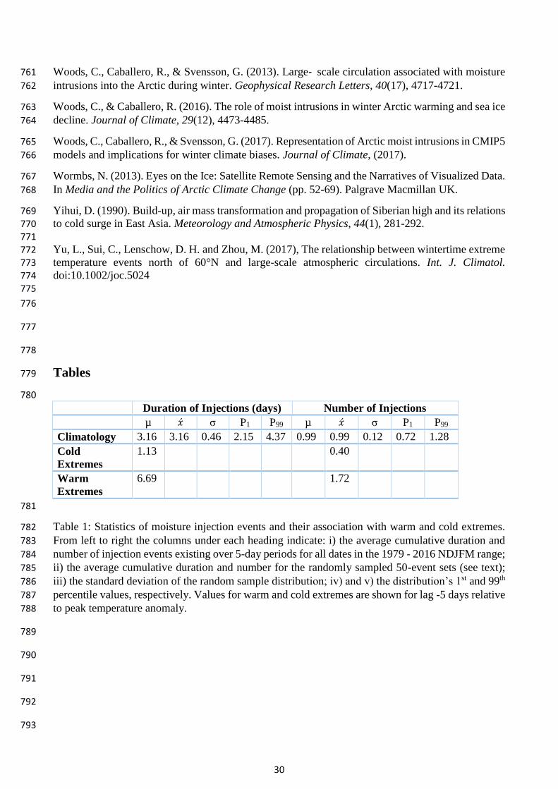
Duration of Injections (days) Number of Injections

µ �́� σ P1 P99 µ �́� σ P1 P99

Climatology 3.16 3.16 0.46 2.15 4.37 0.99 0.99 0.12 0.72 1.28

Cold

Extremes

1.13 0.40

Warm

Extremes

6.69 1.72

781

Table 1: Statistics of moisture injection events and their association with warm and cold extremes. 782

From left to right the columns under each heading indicate: i) the average cumulative duration and 783

number of injection events existing over 5-day periods for all dates in the 1979 - 2016 NDJFM range; 784

ii) the average cumulative duration and number for the randomly sampled 50-event sets (see text); 785

iii) the standard deviation of the random sample distribution; iv) and v) the distribution’s 1st and 99th 786

percentile values, respectively. Values for warm and cold extremes are shown for lag -5 days relative 787

to peak temperature anomaly. 788

789

790

791

792

793

31

794

795

796

797

798

799

800

801

802

803

804

805

Figure Captions 806

Figure 1: Timing of the Arctic cold and warm extremes in the (a) ERA-Interim and (b) NCEP/NCAR 807

reanalyses, defined as described in Section 2.2. Over the period 1979-2016 the top 50 events are 808

selected for both datasets. An additional 38 events are shown for NCEP/NCAR over the period 1950-809

1979. c) PDF of month of occurrence of warm (red) and cold (blue) Arctic extremes in the ERA-810

Interim reanalysis. 811

Figure 2: Composite 2-metre temperature anomalies (K) for (a-c) warm and (d-f) cold extremes at 812

lags of (a, d) -5, (b, e) 0 and (c, f) +5 days relative to peak temperature anomaly. Corresponding 813

composite downward thermal radiation (Wm-2) at lags of (g, j) -5, (h, k) 0 and (i, l) +5 days relative 814

to peak temperature anomaly. Only statistically significant anomalies are shown; cross-hatching 815

marks regions of high sign agreement (see Section 2.1). 816

Figure 3: Composite sea-level pressure anomalies (hPa) for (a-c) warm and (d-f) cold extremes at 817

lags of (a, d) -5, (b, e) 0 and (c, f) +5 days relative to peak temperature anomaly. Corresponding 818

absolute sea-level pressure composites (hPa) at lags of (g, j) -5, (h, k) 0 and (i, l) +5 days relative to 819

peak temperature anomaly. In panels (a-f), only statistically significant anomalies are shown; cross-820

hatching marks regions of high sign agreement (see Section 2.1). The green line in b) corresponds to 821

the transects shown in Figs. 5-8. 822

Figure 4: Composite 500 hPa geopotential height anomalies (m) for warm and cold extremes at lags 823

of (a, d) -5, (b, e) 0 and (c, f) +5 days relative to peak temperature anomaly. Corresponding composite 824

300 hPa wind (vectors) and windspeed (ms-1, colours) anomalies at lags of (g, j) -5, (h, k) 0 and (i, l) 825

+5 days relative to peak temperature anomaly. Only statistically significant anomalies are shown; 826

cross-hatching marks regions of high sign agreement (see Section 2.1). 827

Figure 5: Composite transects for warm extremes. The transect line is shown in Fig. 3a; Scandinavia 828

is to the left and the Bering Strait to the right. Shading shows absolute temperature (left column) and 829

temperature anomaly (right). Arrows show the component of the absolute wind (left column) and 830

32

anomalous wind (right) in the plane of the transect, with horizontal and vertical velocities scaled 831

appropriately for the axes. White contours in the left column show potential temperature (contour 832

interval of 4 K). 833

Figure 6: As in Figure 5 but with shading showing humidity (left column) and humidity anomaly 834

(right). Magenta lines in left column show cloud fraction, contoured at 30% (thin), 50% (medium) 835

and 70% (thick). Magenta lines in right column show cloud fraction anomaly, contoured at +20% 836

(solid) and –20% (dashed). 837

Figure 7: As in Figure 5 but for the cold extremes 838

Figure 8: As in Figure 6 but for the cold extremes. 839

Figure 9: Mean injection event duration (a) and frequency (b) integrated over 5-day windows, for all

injection events which existed for at least one timestep over lags -22 to 12 days relative to the 50

warm (red) and cold (blue) temperature extremes. The x-axis marks lags relative to the peak

temperature anomaly; values are shown as a function of the central day of each window. Dashed lines

indicate the 1st and 99th percentile values of the two metrics, obtained from random sampling, as well

as their means.

Figure 10: Shading shows (a) climatological density of intrusion centroid trajectories per moisture 840

injection event; (b) anomalies with respect to (a) for all injection events which existed for at least one 841

timestep between 7 to 3 days before the warm extremes; (c) same as (b) but for the cold extremes. 842

Trajectory densities are calculated by dividing the study region into 350 km × 350 km grid boxes and 843

counting the number of 6-hourly centroid trajectory points contained within each grid box. Arrows in 844

(a) indicate the typical direction in which the intrusion centroid trajectories move. They are computed 845

as the unit tangent vector at each time step along each centroid trajectory; the tangent vectors falling 846

within each grid box are then averaged. If the trajectories are isotropic the arrows average to zero. 847

Arrows in (b) and (c) show the vector differences between the warm and cold extremes and the 848

climatology in (a), respectively. Shading and arrows in (b) and (c) are shown only for anomalies 849

significant at the 2% level. Dashed lines show the 70° N and 80° N parallels. 850

Figure 11: Climatological frequencies of (a) cyclones (b) cyclogenesis and (c) cyclolysis for NDJFM 851

based on the cyclone detection algorithm of Hanley and Caballero (2012). Mean anomalies over the 852

5 days prior to 30 warm extremes of (d) cyclone frequency (e) cyclogenesis and (f) cyclolysis. (g-i) 853

Same as (a-c) but for 28 cold extremes. The thick dashed contour in (b) shows the climatological 854

NDJFM sea-ice margin (15% sea-ice concentration) in ERA-Interim. Thin dashed lines show the 70° 855

N and 80° N (a-i) and 85° N (a) parallels. Frequencies are computed by counting the number of 856

features within a radius of 564 km (equivalent to 5° latitude) of each point on a 3° × 3° spherical grid. 857

The area enclosed by the 85° N parallel is approximately equal to the area of a circle with radius 564 858

km. 859

Figure 12: Mean frequency over 30 warm extremes of (a) cyclones (b) cyclogensis and (c) cyclolysis; 860

for the cyclones which existed north of 80° N for at least one timestep during the 5 days prior to each 861

warm extreme. Dashed lines show the 70° N and 80° N parallels. 862

Figure 13: (a-e) Composite anomalies of cyclone frequency (shading) and intrusion density (contours) 863

for 30 warm extremes at lags of (a) -10 to -8, (b) -8 to -6, (c) -6 to -4; (d) -4 to -2 and (e) -2 to 0 days 864

relative to peak warmth. (f) For comparison, climatological intrusion density plotted in the same units 865

as in the other panels. Contours in (a-e) begin at 0.4 (thickest contour) and increase by 0.15. Dashed 866

lines show the 70° N and 80° N parallels. 867

33

Figure 14. Projections of the (a) warm and (b) cold spells onto the NAO (red) and AO (black) indices. 868

Projections of the (c) warm and (d) cold spells on a standard Siberian High index (red) and a Siberian 869

High index with the reference domain shifted to the North (black). The dashed horizontal lines in all 870

panels mark the one-sided 5% significance levels. 871

Figure 15: a) Timing of the Arctic warm extremes (red bars) and Eurasian cold extremes (blue bars). 872

The top 50 events for both classes are selected over the period 1979-2016. The blue line is the 873

Northern Eurasian temperature index (NETI, see Section 6). b) Scatterplot of all negative NETI 874

episodes vs. the corresponding Arctic temperature anomalies (blue circles); all the positive Arctic 875

anomalies vs. the corresponding NETI values (red circles); all the cold Eurasian extremes vs. the 876

corresponding Arctic temperature anomalies (blue filled circles); all the warm Arctic extremes vs. the 877

corresponding NETI values (red filled circles). Note that the warm and cold anomalies have been 878

selected enforcing a minimum 7-day separation and excluding warmer/colder days, as described in 879

Section 3. The red horizontal lines mark the mean (continuous) and median (dashed) NETI value 880

corresponding to warm Arctic extremes. The blue vertical lines mark the mean (continuous) and 881

median (dashed) Arctic temperature anomaly corresponding to cold Eurasian extremes. 882

883

884

885

886

Figures 887

888

34

889

Figure 1: Timing of the Arctic cold and warm extremes in the (a) ERA-Interim and (b) NCEP/NCAR 890

reanalyses, defined as described in Section 2.2. Over the period 1979-2016 the top 50 events are 891

selected for both datasets. An additional 38 events are shown for NCEP/NCAR over the period 1950-892

1979. c) PDF of month of occurrence of warm (red) and cold (blue) Arctic extremes in the ERA-893

Interim reanalysis. 894

895

896

897

35

898

36

Figure 2: Composite 2-metre temperature anomalies (K) for (a-c) warm and (d-f) cold extremes at 899

lags of (a, d) -5, (b, e) 0 and (c, f) +5 days relative to peak temperature anomaly. Corresponding 900

composite downward thermal radiation (Wm-2) at lags of (g, j) -5, (h, k) 0 and (i, l) +5 days relative 901

to peak temperature anomaly. Only statistically significant anomalies are shown; cross-hatching 902

marks regions of high sign agreement (see Section 2.1). 903

904

905

37

906

38

Figure 3: Composite sea-level pressure anomalies (hPa) for (a-c) warm and (d-f) cold extremes at 907

lags of (a, d) -5, (b, e) 0 and (c, f) +5 days relative to peak temperature anomaly. Corresponding 908

absolute sea-level pressure composites (hPa) at lags of (g, j) -5, (h, k) 0 and (i, l) +5 days relative to 909

peak temperature anomaly. In panels (a-f), only statistically significant anomalies are shown; cross-910

hatching marks regions of high sign agreement (see Section 2.1). The green line in b) corresponds to 911

the transects shown in Figs. 5-8. 912

913

914

39

915

40

Figure 4: Composite 500 hPa geopotential height anomalies (m) for warm and cold extremes at lags 916

of (a, d) -5, (b, e) 0 and (c, f) +5 days relative to peak temperature anomaly. Corresponding composite 917

300 hPa wind (vectors) and windspeed (ms-1, colours) anomalies at lags of (g, j) -5, (h, k) 0 and (i, l) 918

+5 days relative to peak temperature anomaly. Only statistically significant anomalies are shown; 919

cross-hatching marks regions of high sign agreement (see Section 2.1). 920

921

922

923

924

925

926

927

928

929

930

931

932

933

934

935

936

937

938

939

41

940

Figure 5: Composite transects for warm extremes. The transect line is shown in Fig. 3a; Scandinavia 941

is to the left and the Bering Strait to the right. Shading shows absolute temperature (left column) and 942

temperature anomaly (right). Arrows show the component of the absolute wind (left column) and 943

anomalous wind (right) in the plane of the transect, with horizontal and vertical velocities scaled 944

appropriately for the axes. White contours in the left column show potential temperature (contour 945

interval of 4 K). 946

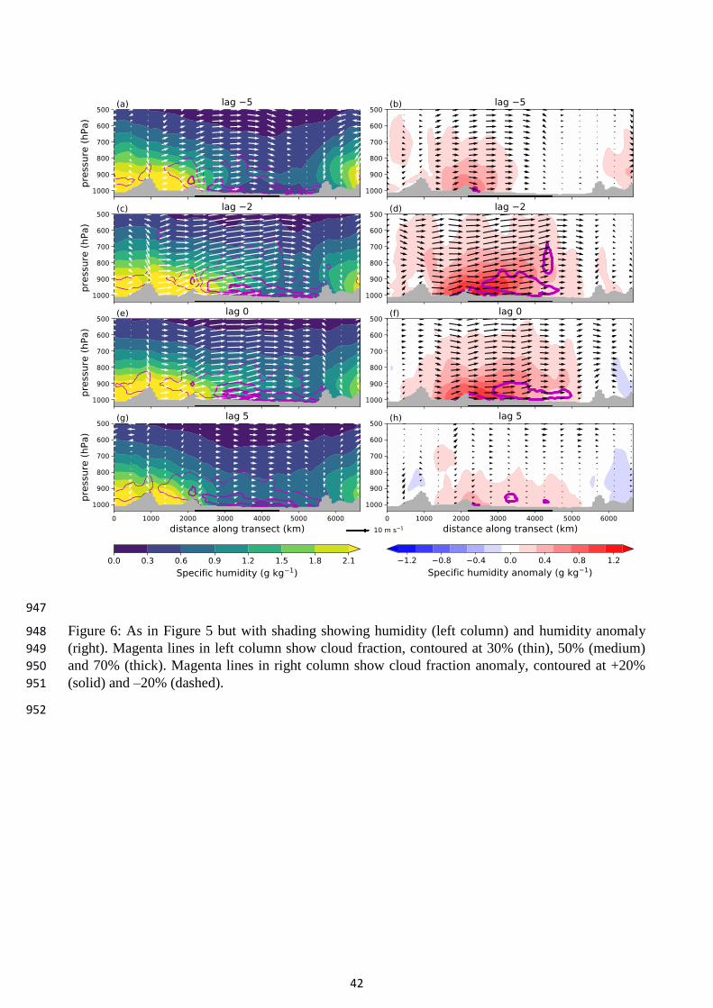
42

947

Figure 6: As in Figure 5 but with shading showing humidity (left column) and humidity anomaly 948

(right). Magenta lines in left column show cloud fraction, contoured at 30% (thin), 50% (medium) 949

and 70% (thick). Magenta lines in right column show cloud fraction anomaly, contoured at +20% 950

(solid) and –20% (dashed). 951

952

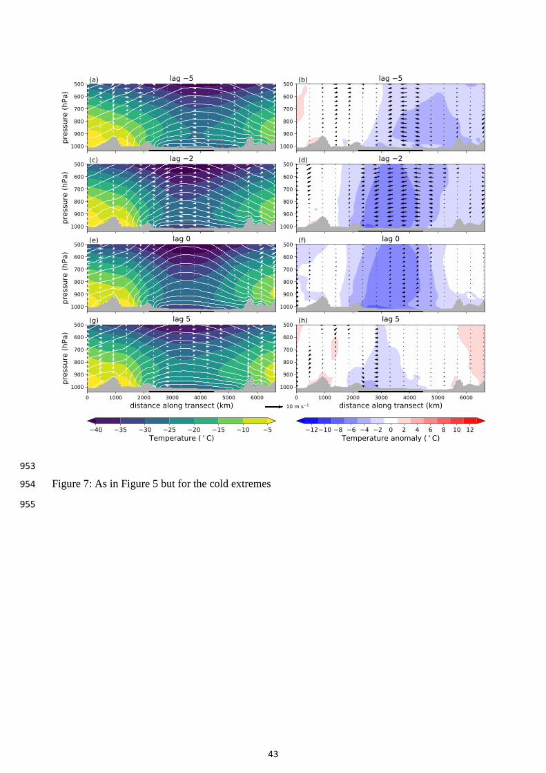
43

953

Figure 7: As in Figure 5 but for the cold extremes 954

955

44

956

Figure 8: As in Figure 6 but for the cold extremes. 957

958

959

960

961

962

963

964

965

966

967

968

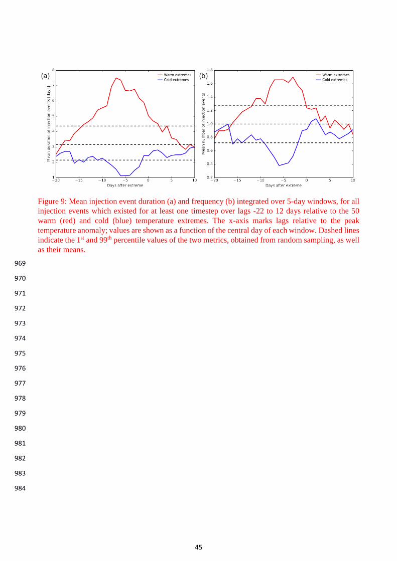
45

969

970

971

972

973

974

975

976

977

978

979

980

981

982

983

984

Figure 9: Mean injection event duration (a) and frequency (b) integrated over 5-day windows, for all

injection events which existed for at least one timestep over lags -22 to 12 days relative to the 50

warm (red) and cold (blue) temperature extremes. The x-axis marks lags relative to the peak

temperature anomaly; values are shown as a function of the central day of each window. Dashed lines

indicate the 1st and 99th percentile values of the two metrics, obtained from random sampling, as well

as their means.

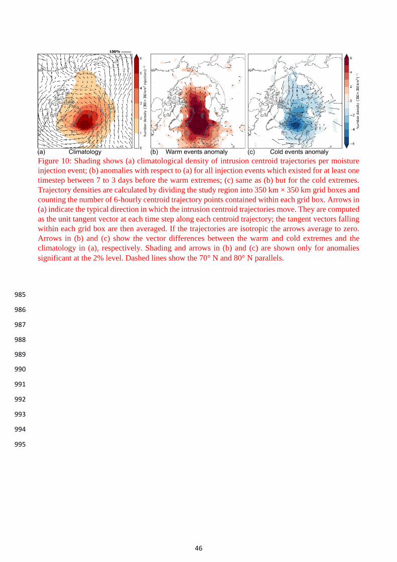
46

985

986

987

988

989

990

991

992

993

994

995

Figure 10: Shading shows (a) climatological density of intrusion centroid trajectories per moisture

injection event; (b) anomalies with respect to (a) for all injection events which existed for at least one

timestep between 7 to 3 days before the warm extremes; (c) same as (b) but for the cold extremes.

Trajectory densities are calculated by dividing the study region into 350 km × 350 km grid boxes and

counting the number of 6-hourly centroid trajectory points contained within each grid box. Arrows in

(a) indicate the typical direction in which the intrusion centroid trajectories move. They are computed

as the unit tangent vector at each time step along each centroid trajectory; the tangent vectors falling

within each grid box are then averaged. If the trajectories are isotropic the arrows average to zero.

Arrows in (b) and (c) show the vector differences between the warm and cold extremes and the

climatology in (a), respectively. Shading and arrows in (b) and (c) are shown only for anomalies

significant at the 2% level. Dashed lines show the 70° N and 80° N parallels.

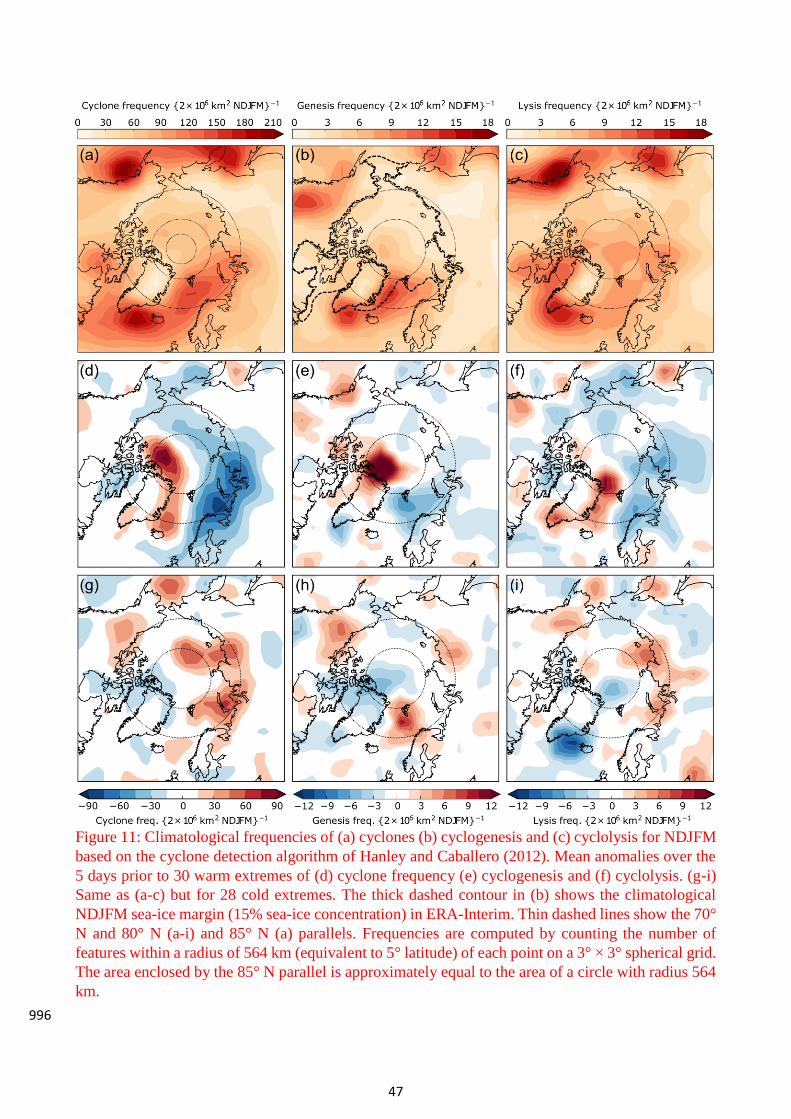
47

996

Figure 11: Climatological frequencies of (a) cyclones (b) cyclogenesis and (c) cyclolysis for NDJFM

based on the cyclone detection algorithm of Hanley and Caballero (2012). Mean anomalies over the

5 days prior to 30 warm extremes of (d) cyclone frequency (e) cyclogenesis and (f) cyclolysis. (g-i)

Same as (a-c) but for 28 cold extremes. The thick dashed contour in (b) shows the climatological

NDJFM sea-ice margin (15% sea-ice concentration) in ERA-Interim. Thin dashed lines show the 70°

N and 80° N (a-i) and 85° N (a) parallels. Frequencies are computed by counting the number of

features within a radius of 564 km (equivalent to 5° latitude) of each point on a 3° × 3° spherical grid.

The area enclosed by the 85° N parallel is approximately equal to the area of a circle with radius 564

km.

48

997

998

999

1000

1001

1002

1003

1004

1005

1006

1007

1008

1009

1010

1011

1012

1013

1014

1015

1016

1017

1018

1019

Figure 12: Mean frequency over 30 warm extremes of (a) cyclones (b) cyclogensis and (c) cyclolysis;

for the cyclones which existed north of 80° N for at least one timestep during the 5 days prior to each

warm extreme. Dashed lines show the 70° N and 80° N parallels.

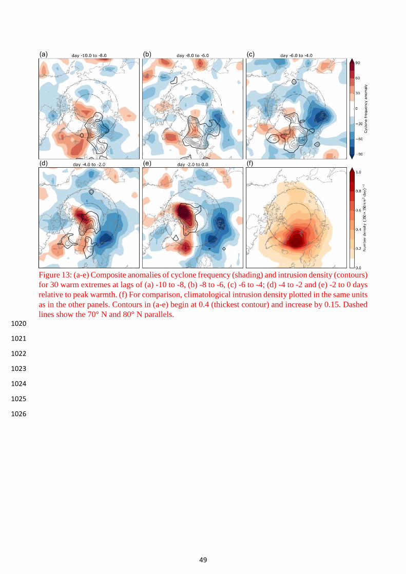
49

1020

1021

1022

1023

1024

1025

1026

Figure 13: (a-e) Composite anomalies of cyclone frequency (shading) and intrusion density (contours)

for 30 warm extremes at lags of (a) -10 to -8, (b) -8 to -6, (c) -6 to -4; (d) -4 to -2 and (e) -2 to 0 days

relative to peak warmth. (f) For comparison, climatological intrusion density plotted in the same units

as in the other panels. Contours in (a-e) begin at 0.4 (thickest contour) and increase by 0.15. Dashed

lines show the 70° N and 80° N parallels.

50

1027

Figure 14. Projections of the (a) warm and (b) cold spells onto the NAO (red) and AO (black) indices. 1028

Projections of the (c) warm and (d) cold spells on a standard Siberian High index (red) and a Siberian 1029

High index with the reference domain shifted to the North (black). The dashed horizontal lines in all 1030

panels mark the one-sided 5% significance levels. 1031

1032

1033

1034

1035

1036

1037

1038

51

1039 Figure 15: a) Timing of the Arctic warm extremes (red bars) and Eurasian cold extremes (blue bars). 1040

The top 50 events for both classes are selected over the period 1979-2016. The blue line is the 1041

Northern Eurasian temperature index (NETI, see Section 6). b) Scatterplot of all negative NETI 1042

episodes vs. the corresponding Arctic temperature anomalies (blue circles); all the positive Arctic 1043

anomalies vs. the corresponding NETI values (red circles); all the cold Eurasian extremes vs. the 1044

corresponding Arctic temperature anomalies (blue filled circles); all the warm Arctic extremes vs. the 1045

corresponding NETI values (red filled circles). Note that the warm and cold anomalies have been 1046

selected enforcing a minimum 7-day separation and excluding warmer/colder days, as described in 1047

Section 3. The red horizontal lines mark the mean (continuous) and median (dashed) NETI value 1048

corresponding to warm Arctic extremes. The blue vertical lines mark the mean (continuous) and 1049

median (dashed) Arctic temperature anomaly corresponding to cold Eurasian extremes. 1050

1051

1052

1053

1054

1055

1056

1057