On the distribution of subsidence in the hurricane...

This is an author’s version of an article published in the QUARTERLY JOURNAL OF THE ROYAL METEOROLOGICAL SOCIETY:Q. J. R. Meteorol. Soc. 133: 595–605 (2007) Copyright c 2007 Royal Meteorological SocietyThis work was first published by John Wiley & Sons, Ltd. at www.interscience.wiley.comThe definitive version of this work may be obtained from Wiley Interscience: http://dx.doi.org/10.1002/qj.49

On the distribution of subsidence in the hurricane eyeWayne H. Schubert,a� Christopher M. Rozoff,a Jonathan L. Vigh,a Brian D. McNoldya

and James P. KossinbaColorado State University, USA

bUniversity of Wisconsin, Madison, USA

ABSTRACT: Two hurricane eye features that have yet to be adequately explained are the clear-air moat that forms at theouter edge of the eye and the hub cloud that forms near the circulation centre. To investigate whether these features can beexplained by the spatial distribution of the subsidence field, we have derived an analytical solution of the Sawyer�Eliassentransverse circulation equation for a three-region approximation with an unforced central eye region of intermediate orhigh inertial stability, a diabatically-forced eyewall region of high inertial stability, and an unforced far-field of low inertialstability. This analytical solution isolates the conditions under which the subsidence is concentrated near the edge of theeye. The crucial parameter is the dimensionless dynamical radius of the eye, defined as the physical radius of the eyedivided by the characteristic Rossby length in the eye. When this dimensionless dynamical radius is less than 0.6, there isless than 10% horizontal variation in the subsidence rate across the eye; when it is greater than 1.8, the subsidence rate atthe edge of the eye is more than twice as strong as at the centre of the eye. When subsidence is concentrated at the edgeof the eye, the largest temperature anomalies occur near there rather than at the vortex centre. This warm-ring structure,as opposed to a warm-core structure, is often observed in the lower troposphere of intense hurricanes. Copyright c 2007Royal Meteorological Society

KEY WORDS eyewall; hub cloud; moatReceived 1 September 2006; Revised 2 February 2007; Accepted 6 February 2007

1. Introduction

In reviewing the findings of early hurricane reconnais-sance flights, Simpson and Starrett (1955) presented theschematic reproduced here as Figure 1. They emphasizedthe fact that the hurricane eye often contains low-levelstratocumulus, which takes the form of a ‘hub cloud’ nearthe circulation centre, surrounded by a ‘moat’ of clear airor thin stratocumulus near the outer edge of the eye. Inrecent literature, the term ‘moat’ has been used to describethe radar-echo-free region between the primary eyewalland a concentric eyewall at larger radius. Our discussionhere is limited to the original Simpson�Starrett moat (orinner moat), as opposed to the outer moat that occursbetween concentric eyewalls. The inner-moat structurehas been confirmed by several later studies. For exam-ple, Bundgaard (1958) and Fletcher et al. (1961) presentedU-2 photographs taken from the lower stratosphere look-ing down on the eyes of Typhoon Kit (14 November 1957)and Typhoon Ida (25 September 1958). One of the Idaphotographs, taken just after rapid deepening to 877 hPa(Jordan, 1959), is reproduced here as Figure 2. It showslow-level stratocumulus in the eye, with cloud tops near2250m. Of particular interest is the moat of cloud-freeair at the edge of the eye, which is consistent with theSimpson�Starrett schematic. Bundgaard’s interpretation

�Correspondence to: Wayne H. Schubert, Department of AtmosphericScience, Colorado State University, Fort Collins, Colorado 80523-1371,USA. E-mail: [email protected]

of such features was that ‘downdraughts of hot air hadgouged out these moats at the eyewall’s very edge’.

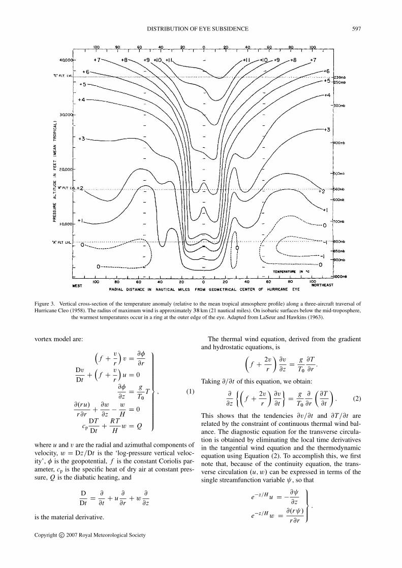
By 1958, aircraft instrumentation and data-recordingtechnology had advanced to a state where it was possibleto obtain data from three aircraft operating simultaneouslyat different levels in Hurricane Cleo. Based on these data,LaSeur and Hawkins (1963) constructed the temperatureanomaly cross-section reproduced here as Figure 3. At thistime Cleo had maximum winds of 46m s�1 at a radius of38 km (21 nautical miles). A striking feature revealed byFigure 3 is that the warmest temperatures in the eye atmiddle and lower levels occur in a ring at the outer edge ofthe eye. The figure also suggests a transition from a lower-tropospheric warm-ring structure to an upper-troposphericwarm-core structure.

With the amount of aircraft reconnaissance data accu-mulated during the 1960s, it became possible to performcomposite analyses. A particularly insightful study wasthat of Gray and Shea (1973), who produced a 21-stormcomposite analysis of the hurricane inner core region.Their composite vertical motion diagram, reproduced hereas the top panel in Figure 4, shows a couplet of strongupward and downward motion with the peak downdraughtlocated just inside the main updraught core. As a summaryof their composite analysis, Gray and Shea noted that thelargest upward motions occur very close to the radius ofmaximum wind and that the highest temperatures occurjust inside the eyewall, corresponding to the large subsi-dence warming that occurs at that radius.

Copyright c 2007 Royal Meteorological Society

596 W. H. SCHUBERT ET AL.

Figure 1. Schematic diagram of the eye of Hurricane Edna, 9–10September 1954. Of particular interest is the ‘hub’ cloud near thecirculation centre and the clear ‘moat’ at the edge of the eye. Adapted

from Simpson and Starrett (1955).

5 km

Figure 2. U-2 photograph looking down from the lower stratosphere onthe eye of Typhoon Ida, 25 September 1958. The moat of clear air atthe edge of the eye is indicative of the strong subsidence there. Adapted

from Fletcher et al. (1961).

After acquisition of the two NOAA WP-3D aircraft inthe late 1970s, it became possible to kinematically com-pute vertical velocity from more accurate aircraft mea-surements of the horizontal motion, provided that coor-dinated radial profiles at several heights were obtained.Based on Hurricane Allen aircraft data (5 August 1980) atthe six flight levels shown in the bottom panel of Figure 4,Jorgensen (1984) kinematically computed the mesoscalevertical velocity from radial velocity measurements using

the axisymmetric form of the mass continuity equation.His results, shown as isolines of the physical-space ver-tical velocity, indicate a 10 km-wide eyewall updraughtwith 7m s�1 peak upward motion and a confined regionof 3m s�1 downdraughts just inside the eyewall.

Some recent three-dimensional nested-grid simulationshave used horizontal grid spacing capable of resolving theeye structures discussed above. One example is a nested-grid simulation of Hurricane Andrew (1992) produced byYau et al. (2004) using an inner grid with 2 km horizon-tal spacing. A radial-height section of the azimuthally-averaged vertical velocity (their figure 6a, not reproducedhere), at a time when the simulated hurricane had low-level winds of approximately 70m s�1, revealed an eye-wall updraught of 3:5m s�1 at z D 7 km and a deep, nar-row downdraught along the inner edge of the eyewall.Malkus (1958) and Zhang et al. (2002) have emphasizedthe role that evaporative and sublimative cooling may playin producing such deep, narrow downdraughts. In con-trast, the argument presented in this paper ignores suchcooling effects in order to isolate other purely dynamicalaspects of the problem.

The purpose of this paper is to present a simple theo-retical argument that isolates the conditions under whichthe subsidence and the warmest temperature anomalies areconcentrated near the outer edge of the eye. The theoreti-cal argument is based on the balanced vortex model and, inparticular, on the associated Sawyer�Eliassen transversecirculation equation (e.g., Ooyama, 1969; Shapiro andWilloughby, 1982; Schubert and Hack, 1982). This argu-ment complements previous studies (e.g., Malkus, 1958;Kuo, 1959; Smith, 1980; Emanuel, 1997; Willoughby,1998) that did not explicitly used the transverse circula-tion equation. The paper is organized as follows. The bal-anced vortex model is presented in Section 2. In Section 3,idealized solutions of the transverse circulation equationare derived. These solutions illustrate how the downwardmass flux in the eye depends on the eyewall geometryand the radial distribution of inertial stability. Section 4presents general numerical solutions of the transverse cir-culation equation, in order to evaluate results derived fromthe more strict assumptions in Section 3. Observationsof two intense hurricanes, Guillermo and Isabel, whichshow striking evidence of a warm-ring structure associ-ated with strong subsidence at the outer edge of the eye,are presented in Section 5. A summary of the results andconclusions is given in Section 6.

2. The balanced vortex model

We consider inviscid, axisymmetric, quasi-static,gradient-balanced motions of a stratified, compressibleatmosphere on an f -plane. As the vertical coordinatewe use z D H log.p0=p/, where H D RT0=g is theconstant scale height, and where p0 and T0 are constantreference values of pressure and temperature. We choosep0 D 100 kPa and T0 D 300K, the latter of which yieldsH � 8:79 km. The governing equations for the balanced


DISTRIBUTION OF EYE SUBSIDENCE 597

Figure 3. Vertical cross-section of the temperature anomaly (relative to the mean tropical atmosphere profile) along a three-aircraft traversal ofHurricane Cleo (1958). The radius of maximum wind is approximately 38 km (21 nautical miles). On isobaric surfaces below the mid-troposphere,

the warmest temperatures occur in a ring at the outer edge of the eye. Adapted from LaSeur and Hawkins (1963).

vortex model are:�

f Cv

r

�

v D@�

@rDvDt

C�

f Cv

r

�

u D 0

@�

@zD

g

T0

T

@.ru/

r@rC@w

@z�w

HD 0

cpDTDt

CRT

Hw D Q

9

>

>

>

>

>

>

>

>

>

>

>

>

>

=

>

>

>

>

>

>

>

>

>

>

>

>

>

;

; (1)

where u and v are the radial and azimuthal components ofvelocity, w D Dz=Dt is the ‘log-pressure vertical veloc-ity’, � is the geopotential, f is the constant Coriolis par-ameter, cp is the specific heat of dry air at constant pres-sure, Q is the diabatic heating, and

DDt

D@

@tC u

@

@rC w

@

@z

is the material derivative.

The thermal wind equation, derived from the gradientand hydrostatic equations, is

�

f C2v

r

�

@v

@zD

g

T0

@T

@r:

Taking @=@t of this equation, we obtain:

@

@z

²�

f C2v

r

�

@v

@t

³

Dg

T0

@

@r

�

@T

@t

�

: (2)

This shows that the tendencies @v=@t and @T=@t arerelated by the constraint of continuous thermal wind bal-ance. The diagnostic equation for the transverse circula-tion is obtained by eliminating the local time derivativesin the tangential wind equation and the thermodynamicequation using Equation (2). To accomplish this, we firstnote that, because of the continuity equation, the trans-verse circulation .u; w/ can be expressed in terms of thesingle streamfunction variable , so that

e�z=Hu D �@

@z

e�z=Hw [email protected] /

r@r

9

>

>

=

>

>

;

:



Figure 4. The top panel, adapted from Gray and Shea (1973), displaysisolines of the vertical p-velocity, composited with respect to the radiusof maximum wind. The bottom panel, adapted from Jorgensen (1984),displays isolines of the physical-space vertical velocity for HurricaneAllen (5 August 1980). In both diagrams the vertical velocity has been

computed kinematically from aircraft measurements of radial wind.

We next multiply the tangential wind equation by� .f C 2v=r/ and the thermodynamic equation by g=T0,and write the resulting equations as

�

�

f C2v

r

�

@v

@tC B

@.r /

r@rC C

@

@zD 0; (3)

andg

T0

@T

@tC A

@.r /

r@rC B

@

@zD

g

cpT0

Q; (4)

where the static stability A, the baroclinity B and theinertial stability C are defined by

A D ez=H g

T0

�

@T

@zC�T

H

�

; (5)

B D �ez=H

�

f C2v

r

�

@v

@zD �ez=H g

T0

@T

@r; (6)

C D ez=H

�

f C2v

r

� �

f [email protected]/

r@r

�

: (7)

Adding @=@r of Equation (4) to @=@z of Equation (3), andthen using Equation (2), we obtain the Sawyer�Eliassentransverse circulation equation:

@

@r

�

[email protected] /

r@rC B

@

@z

�

C@

@z

�

[email protected] /

r@rC C

@

@z

�

Dg

cpT0

@Q

@r: (8)

We shall only consider vortices withAC � B2 > 0 every-where, in which case Equation (8) is an elliptic equation.As for boundary conditions on Equation (8), we requirethat vanish at r D 0 and at the bottom and top isobaricsurfaces z D 0, z D zT , and that r ! 0 as r ! 1. Inthe next section we solve a simplified version of Equa-tion ( 8) under these boundary conditions.

3. Solutions of the transverse circulation equation

For real hurricanes the coefficients A, B and C can havecomplicated spatial distributions, which would precludeanalytical solution of Equation (8). To obtain analyticalsolutions, we shall consider an idealized vortex that leadsto a drastic simplification of the coefficients A and B ,but retains the crucial radial dependence of the inertialstability C . Thus, we consider a barotropic vortex (B D0), noting that this assumption means that the radialderivative of T on isobaric surfaces is zero, but that, witha cyclonic vortex, the radial derivative of T on physicalheight surfaces is slightly positive. The static stability isgiven by

A D ez=HN 2;

where the square of the Brunt�Vaisala frequency, N 2, isa constant. The inertial stability (Equation 7) can then bewritten in the form

C D ez=H Of 2;

where

Of .r/ D

²�

f C2v

r

� �


r@r

�³

12;

is the ‘effective Coriolis parameter’. Under the aboveassumptions, (Equation (8)) reduces to

N 2 @

@r

�

@.r /

r@r

�

C Of 2e�z=H @

@z

�

ez=H @

@z

�

Dge�z=H

cpT0

@Q

@r: (9)

Assuming that the diabatic heating Q.r; z/ and thestreamfunction .r; z/ have the separable forms

Q.r; z/ D OQ.r/ exp� z

2H

�

sin�

�z

zT

�

;

.r; z/ D O .r/ exp�

�z

2H

�

sin�

�z

zT

�

;

the partial differential equation (9) reduces to the ordinarydifferential equation:

r2 d2 O

dr2C r

d O

dr�

�

�2r2 C 1�

O Dgr2

cpT0N 2

d OQ

dr; (10)

where

�2 DOf 2

N 2

²

�2

z2T

C1

.2H/2

³



is the inverse Rossby length squared. Here we are par-ticularly interested in the important role played by radialvariations of Of , and hence radial variations of �. To treatradial variations of Of and � in a simple manner, we con-sider the specific barotropic vortex in which the azimuthalwind is given by the following formulae:� If 0 � r � r1 (eye):

2rv.r/ D�

Of0 � f�

r2: (11)

� If r1 � r � r2 (eyewall):

2rv.r/ D°

Of 20 r

41 C Of 2

1

�

r4 � r41

�

±

12

� f r2: (12)

� If r2 � r < 1 (far-field):

2rv.r/ D°

Of 20 r

41 C Of 2

1

�

r42 � r4

1

�

C Of 22

�

r4 � r42

�

±

12

� f r2: (13)

Here r1 and r2 are specified constants giving the inner andouter radii of the eyewall. From Equations (11)–(13) wecan easily show that

Of .r/ D

²�

f C2v

r

� �


r@r

�³

12

D

8

ˆ

<

ˆ

:

Of0 if 0 � r < r1 (eye)Of1 if r1 < r < r2 (eyewall) ,Of2 if r2 < r < 1 (far-field)

(14)

so that Of0, Of1 and Of2 can be interpreted as specifiedconstants giving the effective Coriolis parameters in theeye, eyewall, and far-field. Because of Equation (14),the inverse Rossby length �.r/ also has the piecewise-constant form:

�.r/ DOf .r/

N

�

�2

z2T

C1

4H 2

�

12

D

8

ˆ

<

ˆ

:

�0 if 0 � r < r1 (eye)�1 if r1 < r < r2 (eyewall) ,�2 if r2 < r < 1 (far-field)

(15)

where the constants �0, �1 and �2 are defined in terms ofthe constants Of0, Of1 and Of2 through Equation (14) and thesecond equality in Equation (15). Plots of v.r/, computedfrom Equations (11)–(13) using the parameters listed inTable I, are shown in Figure 5(a). In constructing this tableand this figure we have used f D 5 � 10�5 s�1 and

N

f

²

�2

z2T

C1

4H 2

³�12

D 1000 km:

Note that the four v.r/ profiles, denoted by cases A�D,all have v.r2/ D 70m s�1. Cases B and D are U-shaped,

so that there is relatively high vorticity in the eyewall andrelatively low vorticity in the eye. In contrast, cases Aand C are Rankine-like, with equal vorticity in the eyeand eyewall. The Rossby length in the eye, given by ��1

0

and listed in the seventh column of the table, is smallfor the Rankine-like vortices A and C. As a consequence,the (dimensionless) dynamical size of the eye, given by�0r1 and listed in the eighth column, is large for theRankine-like vortices A and C, whereas it is small forthe U-shaped vortices B and D. In a crude sense, theRankine-like profiles A and C can be envisioned as havingevolved respectively from the U-shaped profiles B andD via potential vorticity mixing (Schubert et al., 1999;Kossin and Eastin, 2001; Kossin and Schubert, 2001;Kossin et al., 2002; Montgomery et al., 2002). Note thatin the transformations B ! A and D ! C, the physicalradius of the eye does not change but the dynamical radiusof the eye increases by more than a factor of three for B! A and by nearly a factor of five for D ! C. This effectis crucial in later discussions.

We now assume that the diabatic heating has thepiecewise-constant form

OQ.r/ D

8

ˆ

<

ˆ

:

0 if 0 � r < r1 (eye)Q1 if r1 < r < r2 (eyewall) ,0 if r2 < r < 1 (far-field)

(16)

where Q1 is a constant. This structure represents theheating that occurs when moist updraughts are confined toan annular eyewall. Only two of the three parameters r1,r2 andQ1 are independently varied. The three parametersare constrained by:

Q1

cp

�

r22 � r2

1

�

D 125K day�1 .50 km/2: (17)

A crude interpretation of this constraint is that the impliedarea-averaged rainfall is fixed as we vary any two of thethree parameters r1, r2 and Q1. Such latent heating ratesare supported by the satellite-derived measurements ofRodgers et al. (1998).

Because of Equation (16), the right-hand side of Equa-tion (10) vanishes everywhere except at the points r D r1

Table I. Vortex parameters: radius of inner edge of eyewall (r1); radiusof outer edge of eyewall (r2); effective Coriolis parameter in eye( Of0=f ), eyewall ( Of1=f ), and far-field ( Of2=f ); Rossby length in eye(��1

0); dynamic radius of eye (�0r1); proportion of downward mass

flux occurring in eye (�).

Case r1 r2Of0=f Of1=f Of2=f ��1

0�0 r1 �

(km) (km) (km) (%)

A 10 20 141.0 141.0 1.0 7:1 1.41 12.6B 10 20 41.0 145.2 1.0 24.4 0.41 14.7C 30 40 71.0 71.0 1.0 14.1 2.13 13.5D 30 40 14.3 85.3 1.0 69.9 0.43 21.1



Figure 5. (a) Plots of v.r/, computed from Equations (11)–(13), usingthe parameter values listed in Table I. (b) Corresponding radially-dependent part of vertical log-pressure velocities given by Equa-tion (24). (c) Corresponding temperature tendencies obtained from

Equations (25)–(27).

and r D r2. At these points, the differential equation (10)is replaced by the two jump conditions

"

d.r O /

r dr

#rC

1

r�1

DgQ1

cp T0N 2

"

d.r O /

r dr

#rC

2

r�2

D �gQ1

cp T0N 2

9

>

>

>

>

>

>

>

=

>

>

>

>

>

>

>

;

; (18)

which can be derived by integrating Equation (10) acrossnarrow intervals straddling the points r D r1 and r D r2.Assuming Equation (16), the solution of the ordinarydifferential equation (10) consists of linear combinationsof the first-order modified Bessel functions I1.�r/ andK1.�r/ in each of the three regions. These modifiedBessel functions are shown by the dashed curves inFigure 6. Because our boundary condition requires thatO D 0 at r D 0, we can discard the K1.�r/ solution in

the inner region. Similarly, because r O ! 0 as r ! 1,we can discard the I1.�r/ solution in the outer region.

The solution of Equation (10) can then be written as

O .r/ D

8

ˆ

ˆ

ˆ

ˆ

ˆ

ˆ

ˆ

<

ˆ

ˆ

ˆ

ˆ

ˆ

ˆ

ˆ

:

O 1

I1.�0r/

I1.�0r1/0 � r � r1

O 1F.r; r2/C O 2F.r1; r/

F.r1; r2/r1 � r � r2 ;

O 2

K1.�2r/

K1.�2r2/r2 � r < 1

(19)where

F.x; y/ D I1.�1x/K1.�1y/ � K1.�1x/ I1.�1y/

and O 1 and O 2 are constants to be determined by the twojump conditions (18). Note that Equation (19) guaranteesthat O .r/ is continuous at r D r1 and r D r2.

The vertical motion field can be obtained from thestreamfunction (Equation (19)) via differentiation, usingthe relations

d®

rI1.�r/¯

rdrD �I0.�r/

d®

rK1.�r/¯

rdrD ��K0.�r/

9

>

>

=

>

>

;

;

where I0.�r/ and K0.�r/ are the zeroth-order modifiedBessel functions (shown by the solid curves in Figure 6).Thus, from differentiation of Equation (19) we obtain:

d.r O /

r drD

8

ˆ

ˆ

ˆ

ˆ

ˆ

ˆ

ˆ

<

ˆ

ˆ

ˆ

ˆ

ˆ

ˆ

ˆ

:

O 1�0

I0.�0r/

I1.�0r1/0 � r < r1

O 1�1G.r; r2/ � O 2�1G.r; r1/

F.r1; r2/r1 < r < r2 ;

� O 2�2

K0.�2r/

K1.�2r2/r2 < r < 1

(20)where

G.x; y/ D I0.�1x/K1.�1y/C K0.�1x/ I1.�1y/:

0 0.5 1 1.5 2 2.5 30

0.5

1

1.5

2

2.5

3

3.5

4

x

I n(x),

K n(x)

I0(x) I1(x)K0(x) K1(x)

Figure 6. The first-order modified Bessel functions I1.x/ and K1.x/,from which the streamfunction is constructed, and the zeroth-ordermodified Bessel functions I0.x/ and K0.x/, from which the vertical

motion is constructed.



Use of Equation (20) in the jump conditions (18) leads totwo algebraic equations that determine the constants O 1

and O 2. Solving these two algebraic equations, and withthe aid of the Wronskian

I0.x/K1.x/C K0.x/ I1.x/ D1

x;

we can express O 1 and O 2 as

O 1 DgQ1r2F.r1; r2/

cpT0N 2

�

1 � ˛

1 � ˛ˇ

�

O 2 DgQ1r1F.r1; r2/

cpT0N 2

�

ˇ � 1

1 � ˛ˇ

�

9

>

>

>

=

>

>

>

;

; (21)

where

˛ D �1r1

²

G.r2; r1/ � F.r1; r2/�2K0.�2r2/

�1K1.�2r2/

³

; (22)

and

ˇ D �1r2

²

G.r1; r2/ � F.r1; r2/�0I0.�0r1/

�1I1.�0r1/

³

: (23)

To summarize, the solution of the transverse circulationequation (8), for the barotropic vortex (Equations (11)–(13)) and the diabatic heating (Equation (16)), yields alog-pressure vertical velocity given by:

w.r; z/ D ez=.2H/ sin�

�z

zT

�

�

8

ˆ

ˆ

ˆ

ˆ

ˆ

ˆ

<

ˆ

ˆ

ˆ

ˆ

ˆ

ˆ

:

O 1�0

I0.�0r/

I1.�0r1/0 � r < r1

O 1�1

G.r; r2/

F.r1; r2/� O 2�1

G.r; r1/

F.r1; r2/r1 < r < r2 :

� O 2�2

K0.�2r/

K1.�2r2/r2 < r < 1

(24)

Plots of the radial dependence on the right-hand side ofEquation (24) for cases A�D are shown in Figure 5(b).For the U-shaped vortices B and D, the subsidence rate isnearly uniform in the eye because the dynamic radius ofthe eye is small (0.41 for B and 0.43 for D) – the centre ofthe eye is less than a Rossby length from the eyewall. Forthe Rankine-like vortices A and C, the subsidence rate inthe centre of the eye is considerably reduced because thehigh inertial stability of the eye results in the centre of theeye being more than a Rossby length from the eyewall.From the first line in Equation ( 24) we can see that, onany isobaric surface, the ratio of the subsidence rate at theedge of the eye to the subsidence rate at the centre of theeye is I0.�0r1/, since I0.0/ D 1. From Figure 6 we notethat I0.�0r1/ < 1:1 when �0r1 < 0:6, while I0.�0r1/ >

2 when �0r1 > 1:8. We conclude that there is less than10% horizontal variation in the subsidence rate in the eyewhen the eye is dynamically small (�0r1 < 0:6), whereasthe subsidence rate at the edge of the eye is more than

twice as strong as the subsidence rate in the centre of theeye when the eye is dynamically large (�0r1 > 1:8).

It is of interest to calculate the proportion of the upwardmass flux in the eyewall that turns inward to subside inthe eye and the proportion that turns outward to subsidein the far-field. From the streamfunction solution (Equa-tion (19)), the fractional downward mass flux in the eye(on any isobaric surface) can be expressed as

� Ddownward mass flux in eyetotal downward mass flux

D

Z r1

0

wr drZ r1

0

wr dr C

Z 1

r2

wr dr

D

Z r1

0

d.r O /

drdr

Z r1

0

d.r O /

drdr C

Z 1

r2

d.r O /

drdr

Dr1 O 1

r1 O 1 � r2 O 2

D˛ � 1

˛ C ˇ � 2;

where the final equality follows from the use of Equa-tions (21). From Equations (22) and (23), we see that thevalue of � depends on the five parameters r1, r2, �0, �1

and �2. Values of � for cases A�D are shown in the lastcolumn of Table I. Note that the transformations to vor-tices with high inertial stability cores (i.e. B ! A and D! C) lead to a reduction in the proportion of the down-ward mass flux that occurs in the eye (e.g. 21.1% to 13.5%for D ! C). Thus, the reduction of the subsidence rate atthe centre of the eye means that the proportion of totaldownward mass flux that occurs in the eye is reduced.

The temperature tendency implied by the secondarycirculation can be obtained from Equation (4) withB D 0.After separating off the vertical dependence, we obtain:

@ OT

@tD

OQ

cp�T0N

2

g

d.r O /

rdr:

Using Equations (16) and (20)–(23), we obtain the follow-ing formulae:� If 0 � r � r1:

@ OT

@tDQ1

cp

²

1 �

�

1 � ˛

1 � ˛ˇ

�

�1r2G.r1; r2/

�

�

1 � ˇ

1 � ˛ˇ

�³

I0.�0r/

I0.�0r1/: (25)

� If r1 � r � r2:

@ OT

@tDQ1

cp

²

1 �

�

1 � ˛

1 � ˛ˇ

�

�1r2G.r; r2/

�

�

1 � ˇ

1 � ˛ˇ

�

�1r1G.r; r1/

³

: (26)



� If r2 � r < 1:

@ OT

@tDQ1

cp

²

1 �

�

1 � ˛

1 � ˛ˇ

�

�

�

1 � ˇ

1 � ˛ˇ

�

�1r1G.r2; r1/

³

K0.�2r/

K0.�2r2/: (27)

Plots of @ OT =@t , computed from Equations (25)–(27) forcases A�D, are shown in Figure 5(c). Note that in cases Aand C (dynamically large eyes) the temperature tendencyis more concentrated near the edge of the eye. This isconsistent with the formation of a warm-ring structure instorms with dynamically large eyes. Another interestingfeature of these plots is the large variation of @ OT =@t acrossthe eyewall, even though the diabatic heating OQ.r/ isconstant across it. This can be interpreted as follows. FromEquation (18) and Figure 5(b) it can be seen that themagnitude of the jumps in vertical velocity are the same atr D r1 and r D r2. Thus, with stronger subsidence at theedge of the eye than just outside the eyewall, the upwardmotion in the eyewall region is larger in its outer part thanin its inner part. For example, considering cases A and C,in the outer part of the eyewall region the compensationbetween the .T0N

2=g/˚

d.r O /=.rdr/

term and the OQ=cpterm is nearly complete, while in the inner part of theeyewall region the former of these two terms is only two-thirds of the latter.

4. Numerical solutions

In order to test the limitations of the barotropic vortexassumption that reduces Equation (8) to Equation (9),we produce numerical solutions of Equation (8) usingmultigrid methods (Fulton et al., 1986; Ciesielski et al.,1986) with fine spatial resolution (�r D 250m and�z D187:5m). The diabatic heating Q.r; z/ has the same spa-tial structure as that used in Section 3, except that thediscontinuities at r1 and r2 are replaced by smooth tran-sitions (A cubic interpolation function was used, so thatbothQ.r; z/ and its radial derivative are continuous.) overa radial distance of 3 km. Figure 7 shows the results of twosuch calculations, one for the barotropic vortex (upper-left panel) and one for the baroclinic vortex (upper-rightpanel). These two vortices have the same radial profileof v at the lower boundary. The middle and lower panelsshow the corresponding w and @T=@t fields, respectively.The middle two panels show that baroclinity increasesthe height of the vertical velocity maximum and associ-ated temperature tendency. This vertical shift of the maxi-mum w from the barotropic to baroclinic situation occursbecause the baroclinic vortex has increased (decreased)static stability at lower (upper) levels and decreased iner-tial stability at upper levels. The heights of maximum jwjand @T=@t are also directly proportional to the level ofmaximum heating, which in the present example is locatedin the upper troposphere. Finally, it should be pointed outthat numerical solutions for U-shaped profiles (not shown)

70

60

60

5040

10

20

30

10

20

3040

50

60

1

23

0

-.25

-.5-.75

-1

-.25-.5

0

1

2

3

-.25

-.25

-.5

-.75

-1

5

10

15

20

25

5

10

15

20

Figure 7. Panels (a) and (b) show v.r; z/ for sample barotropic andbaroclinic vortices, respectively. Panels (c) and (d) show the correspond-ing w.r; z/ fields, as determined from numerical solution of Equa-tion (8), with a contour interval of 1 m s�1 in the ascent regions (solidlines) and �0:25 m s�1 in the descent regions (dotted lines). Panels (e)and (f) show the corresponding temperature tendencies @T=@t , with a

contour interval of 5 K h�1.

validate the generality of the dependence of the radial dis-tribution of eye subsidence on the radial profile of inertialstability.

5. Hurricanes Guillermo and Isabel

We now present observations from two intense hurricanesthat support the warm-ring structure found in the theo-retical arguments of Sections 2 and 3. The first exampleis from Hurricane Guillermo, a category-4 eastern-Pacificstorm that was well observed on 2 and 3 August 1997. Fig-ures 8 (a) and (b) show the time-averaged radial profilesof tangential wind, temperature, and dew-point tempera-ture at 700 hPa for 2 and 3 August, where each compositeprofile incorporates 18 and 20 passes, respectively. Fol-lowing Willoughby et al. (1982), each flight pass has beeninterpolated into vortex-centred grids (�r D 0:5 km); thedata are readily available in such a format from NOAA’sHurricane Research Division. On 2 August, the maxi-mum 700 hPa tangential wind is 52:7m s�1 at r D 29 km;on 3 August, the maximum 700 hPa tangential wind is63:0m s�1 at r D 26 km. Thus, Guillermo strengthened



Figure 8. Radial profiles at 700 hPa, from Hurricane Guillermo, of thetime-averaged (a) tangential wind on 2 August (light solid line) and3 August 1997 (heavy solid line), and (b) temperature and dew-pointtemperature on 2 August (light dashed and dotted lines respectively)and 3 August (heavy dashed and dotted lines respectively). (c) Thecorresponding three-region model’s estimate of Guillermo’s 700 hPatangential wind and temperature tendency on 2 August (light solid anddashed lines respectively) and 3 August (heavy solid and dashed lines

respectively).

and its eyewall contracted during this period. A sub-stantial warm-core anomaly of about 5K persisted (Fig-ure 8(b)), but apparent ‘cooling’ at r < 10 km between thetwo intensive observational campaigns on 2 and 3 Augustleads to a warm-ringed structure in the 3 August com-posite. With a saturated eyewall adjacent to a dew-pointdepression of 3:2 ıC near the inner edge of the eyewall,the 3 August composite is consistent with the results ofSitkowsi et al. (2006). On 2 August, the dew-point depres-sion exceeds 6 ıC but is uniform across Guillermo’s eye.

While admitting the three-region model’s inability tocapture the U-shaped structure within Guillermo’s eye,we can still optimize the three-region model’s parame-ters to estimate the temperature tendencies that shouldresult from the balanced circulation of Guillermo. For

2 August, we choose r1 D 22 km, r2 D 29 km, v.r1/ D39:3m s�1, and v.r2/ D 52:7m s�1; for 3 August, wechoose r1 D 20 km, r2 D 26:5 km, v.r1/ D 52m s�1, andv.r2/ D 63m s�1. Figure 8(c) shows the estimated tan-gential wind curves. Incorporating the diabatic heat-ing constraint given by Equation (17) and using Equa-tions (25)–(27), we obtain the temperature tendenciesshown by the heavy and light dashed lines in Figure 8(c).On 3 August, there is a greater tendency for the storm toproduce a warm-ringed structure. However, the radius ofmaximum temperature change is offset from the warm-ringed structure observed on 3 August; this may perhapsbe explained by the analytical model’s simplified vortexgeometry, or by its lack of evaporative and sublimativecooling.

Our second observational example is from HurricaneIsabel, a category-5 Atlantic hurricane. Figure 9 is a stun-ning photograph of the hub cloud in the eye of Isabel on13 September 2003. On this date, the two NOAA WP-3D aircraft collected high-resolution data from multipleeyewall penetrations at altitudes of 2:1 km and 3:7 km.In Figures 10 (a) and (b), we provide two radial pro-files of 1 s flight-level tangential wind at 3:7 km altitudefrom 1948 UTC to 1956 UTC and at 2:1 km altitudefrom 1922 UTC to 1931 UTC, respectively. These windprofiles reveal a large outward tilt of the radius of max-imum wind (See also the cross-sections shown in Belland Montgomery (2007).) The associated temperature anddew-point temperature profiles exhibit evidence of subsi-dence warming and drying inside the eye, particularly nearthe eyewall. Similar patterns appear in nearly all 16 WP-3D sorties on 13 September. These Isabel results implythat the warm-ring structure can extend over a consider-able depth of the lower troposphere. However, it is an openquestion whether it extends into the upper troposphereor gives way to a warm-core upper tropospheric struc-ture. These Isabel profiles also reveal a vorticity struc-ture more complicated than was specified in the three-region model, which assumed that the eye can be char-acterized by a single Rossby length. The tangential wind

Figure 9. The eye of Hurricane Isabel on 13 September 2003. The hubcloud (near the centre of the photo) is surrounded by a moat of clear airor thin stratocumulus. Because of the large eye diameter (60–70 km),the eyewall (12–14 km tops) behind the hub clud (3 km top) appearsonly slightly higher than the hub cloud itself. Photo courtesy of Sim

Aberson.



Figure 10. Radial profiles of 1 s flight-level tangential wind (solid lines),temperature (dashed lines), and dew-point temperature (dotted lines)from Hurricane Isabel on 13 September 2003 at (a) 3:7 km altitude from1948 UTC to 1956 UTC and (b) 2:1 km altitude from 1922 UTC to 1931

UTC.

profiles for Isabel possess a striking U-shaped structurewithin the eye. In fact, the azimuthal wind profiles shownin Figure 10 would be more accurately characterized bya four-region model, with two regions within the eye.For example, at z D 2:1 km (Figure 10(b)) the averagevorticity in the region 0 � r � 21 km is 1:1 � 10�3 s�1,while the average vorticity in the region 21 � r � 31 kmis 5:8 � 10�3 s�1. These values result in approximateRossby lengths for these two regions of 44 km and 8:5 kmrespectively. The small Rossby length in the outer part ofthe eye plays an important role in confining the large tem-perature anomaly to this region. Eye structures in whichthe vorticity and potential vorticity are much smaller nearthe circulation centre may be the result of a partial mix-ing process in which high-potential-vorticity eyewall airis advected inward but not completely to the centre of theeye. In passing, we note that future work should attemptto estimate temperature tendencies from large observa-tional data sets over numerous storms to determine therobustness of the proposed relationship between inertialstability, eye subsidence and temperature tendency.

6. ConclusionsAssuming the eye can be fairly accurately characterizedby a single Rossby length, we have proposed the following

rules:� There is less than 10% horizontal variation in the

subsidence rate in the eye when the ratio of the eyeradius to the Rossby length in the eye is less than 0.6.This tends to occur with small eyes or eyes with lowinertial stability.

� The subsidence rate at the edge of the eye is more thantwice as strong as the subsidence rate in the centre ofthe eye when the ratio of the eye radius to the Rossbylength in the eye is greater than 1.8. This tends to occurwith large eyes or eyes with high inertial stability.An implication of these results is that the existence

of a hub cloud at the centre of the eye, cascadingpileus in the upper troposphere on the edge of the eye(Willoughby, 1998), a clear inner moat in the lower tro-posphere on the edge of the eye, and a warm-ring ther-mal structure, are all associated with strong inertial sta-bility in the eye and a relatively large eye radius. Thus,in some cases, careful inspection of the cloud field canreveal certain aspects of a hurricane’s dynamical struc-ture. However, further research is needed to better under-stand the relative importance of these dynamical effectsand the evaporative�sublimative cooling effects studiedby Malkus (1958) and Zhang et al. (2002).

In closing, important limitations of the idealized frame-work used in this study should be pointed out. First,the balanced model (Equation (1)), and hence the asso-ciated transverse circulation equation (8), filter transientinertia�gravity waves. In real hurricanes and in bothhydrostatic and non-hydrostatic primitive equation mod-els, high-frequency inertia�gravity oscillations can besuperimposed on the slower-time-scale motions that arewell approximated by Equation (1). An interesting exam-ple can be seen in Yamasaki (1983, figure 15), whichshows 15-minute oscillations of the vertical motion fieldin the eye of an axisymmetric non-hydrostatic model.Such inertia�gravity oscillations have peak amplitudesof vertical motion at the centre of the eye, in contrastto the quasi-balanced motions associated with maximumsubsidence at the edge of the eye. Another interestingfeature of primitive equation model simulations is thatintense storms can produce a temperature field that hasa warm-core structure at upper levels but a warm-ringstructure at lower levels (Yamasaki, 1983, figure 10(a);Hausman et al., 2006, figures 5 and 9). An explanation ofsuch a temperature field in terms of the Sawyer�Eliassenequation would presumably involve relaxing some of theassumptions that lead to the simplified equations (9) and(10).

Acknowledgements

We would like to thank Sim Aberson, Michael Black,Paul Ciesielski, Mark DeMaria, Neal Dorst, Scott Fulton,William Gray, Richard Johnson, Kevin Mallen, MichaelMontgomery, Roger Smith, Richard Taft, and an anony-mous reviewer for their advice and comments. Flight-level data sets were provided by the Hurricane Research



Division (HRD) of NOAA’s Atlantic Oceanographic andMeteorological Laboratory. This research was supportedby NASA/TCSP Grant NNG06GA54G and NSF GrantsATM-0332197, ATM-0530884, ATM-0435694 and ATM-0435644.

ReferencesBell MM, Montgomery MT. 2007. Observed structure, evolution and

potential intensity of category five Hurricane Isabel (2003) from 12–14 September. Mon. Wea. Rev. 114: (in press).

Bundgaard RC. 1958. The first flyover of a tropical cyclone. Weather-wise 11: 79–83.

Ciesielski PE, Fulton SR, Schubert WH. 1986. Multigrid solution of anelliptic boundary value problem from tropical cyclone theory. Mon.Wea. Rev. 114: 797–807.

Emanuel K. 1997. Some aspects of hurricane inner-core dynamics andenergetics. J. Atmos. Sci. 54: 1014–1026.

Fletcher RD, Smith JR, Bundgaard RC. 1961. Superior photographicreconnaissance of tropical cyclones. Weatherwise 14: 102–109.

Fulton SR, Ciesielski PE, Schubert WH. 1986. Multigrid methods forelliptic problems: A review. Mon. Wea. Rev. 114: 943–959.

Gray WM, Shea DJ. 1973. The hurricane’s inner core region. II. Thermalstability and dynamic constraints. J. Atmos. Sci. 30: 1565–1576.

Hausman SA, Ooyama KV, Schubert WH. 2006. Potential vorticitystructure of simulated hurricanes. J. Atmos. Sci. 63: 87–108.

Jordan CL. 1959. A reported sea level pressure of 877 mb. Mon. Wea.Rev. 87: 365–366.

Jorgensen DP. 1984. Mesoscale and convective-scale characteristics ofmature hurricanes. Part II: Inner core structure of Hurricane Allen(1980). J. Atmos. Sci. 41: 1287–1311.

Kossin JP, Eastin MD. 2001. Two distinct regimes in the kinematic andthermodynamic structure of the hurricane eye and eyewall. J. Atmos.Sci. 58: 1079–1090.

Kossin JP, McNoldy BD, Schubert WH. 2002. Vortical swirls in hurri-cane eye clouds. Mon. Wea. Rev. 130: 3144–3149.

Kossin JP, Schubert WH. 2001. Mesovortices, polygonal flow patterns,and rapid pressure falls in hurricane-like vortices. J. Atmos. Sci. 58:2196–2209.

Kuo HL. 1959. Dynamics of convective vortices and eye formation. In:The Atmosphere and the Sea in Motion, Bolin B (ed), RockefellerInstitute Press: New York, pp. 413–424.

LaSeur NE, Hawkins HF. 1963. An analysis of hurricane Cleo (1958)based on data from research reconnaissance aircraft. Mon. Wea. Rev.91: 694–709.

Malkus JS. 1958. On the structure and maintenance of the maturehurricane eye. J. Meteor. 15: 337–349.

Montgomery MT, Vladimirov VA, Denissenko PV. 2002. An experi-mental study on hurricane mesovortices. J. Fluid Mech. 471: 1–32.

Ooyama K. 1969. Numerical simulation of the life cycle of tropicalcyclones. J. Atmos. Sci. 26: 3–40.

Rodgers EB, Olson WS, Karyampudi VM, Pierce HF. 1998. Satellite-derived latent heating distribution and environmental influences inHurricane Opal (1995). Mon. Wea. Rev. 126: 1229–1247.

Schubert WH, Hack JJ. 1982. Inertial stability and tropical cyclonedevelopment. J. Atmos. Sci. 39: 1687–1697.

Schubert WH, Montgomery MT, Taft RK, Guinn TA, Fulton SR,Kossin JP, Edwards JP. 1999. Polygonal eyewalls, asymmetric eyecontraction, and potential vorticity mixing in hurricanes. J. Atmos.Sci. 56: 1197–1223.

Shapiro LJ, Willoughby HE. 1982. The response of balanced hurricanesto local sources of heat and momentum. J. Atmos. Sci. 39: 378–394.

Simpson RH, Starrett LG. 1955. Further studies of hurricane structureby aircraft reconnaissance. Bull. Amer. Meteor. Soc. 36: 459–468.

Sitkowsi M, Dolling K, Barnes G. 2006. The rapid intensification ofHurricane Guillermo (1997) as viewed with GPS dropwindsondes.Paper 4B.8 in Proceedings of the 27th Conference on Hurricanes andTropical Meteorology, 24–28 April 2006, Monterey, CA, AmericanMeteorological Society.

Smith RK. 1980. Tropical cyclone eye dynamics. J. Atmos. Sci. 37:1227–1232.

Willoughby HE. 1998. Tropical cyclone eye thermodynamics. Mon.Wea. Rev. 126: 3053–3067.

Willoughby HE, Clos JA, Shoreibah MG. 1982. Concentric eye walls,secondary wind maxima, and the evolution of the hurricane vortex.J. Atmos. Sci. 39: 395–411.

Yamasaki M. 1983. A further study of the tropical cyclone withoutparameterizing the effects of cumulus convection. Papers in Meteor-ology and Geophysics 34: 221–260.

Yau MK, Liu Y, Zhang D-L, Chen Y. 2004. A multiscale numericalstudy of Hurricane Andrew (1992). Part VI: Small-scale inner-corestructures and wind streaks. Mon. Wea. Rev. 132: 1410–1433.

Zhang D-L, Liu Y, Yau MK. 2002. A multiscale numerical study ofHurricane Andrew (1992). Part V: Inner-core thermodynamics. Mon.Wea. Rev. 130: 2745–2763.


On the distribution of subsidence in the hurricane...

Documents

Transcript of On the distribution of subsidence in the hurricane...