On the connection between the conjugate gradient method and quasi-Newton methods on quadratic...

Comput Optim ApplDOI 10.1007/s10589-014-9677-5

On the connection between the conjugate gradientmethod and quasi-Newton methods on quadraticproblems

Anders Forsgren · Tove Odland

Received: 8 February 2013© Springer Science+Business Media New York 2014

Abstract It is well known that the conjugate gradient method and a quasi-Newtonmethod, using any well-defined update matrix from the one-parameter Broyden fam-ily of updates, produce identical iterates on a quadratic problem with positive-definiteHessian. This equivalence does not hold for any quasi-Newton method. We define pre-cisely the conditions on the update matrix in the quasi-Newton method that give rise tothis behavior. We show that the crucial facts are, that the range of each update matrixlies in the last two dimensions of the Krylov subspaces defined by the conjugate gradi-ent method and that the quasi-Newton condition is satisfied. In the framework based ona sufficient condition to obtain mutually conjugate search directions, we show that theone-parameter Broyden family is complete. A one-to-one correspondence between theBroyden parameter and the non-zero scaling of the search direction obtained from thecorresponding quasi-Newton method compared to the one obtained in the conjugategradient method is derived. In addition, we show that the update matrices from theone-parameter Broyden family are almost always well-defined on a quadratic problemwith positive-definite Hessian. The only exception is when the symmetric rank-oneupdate is used and the unit steplength is taken in the same iteration. In this case it isthe Broyden parameter that becomes undefined.

Keywords Conjugate gradient method · Quasi-Newton method · Unconstrainedprogram

A. Forsgren (B) · T. OdlandOptimization and Systems Theory, Department of Mathematics, KTH Royal Institute of Technology,SE-100 44, Stockholm, Swedene-mail: [email protected]

T. Odlande-mail: [email protected]

123

A. Forsgren, T. Odland

1 Introduction

In this paper we examine some well-known methods used for solving unconstrainedoptimization problems and specifically their behavior on quadratic problems. A moti-vation why these problems are of interest is that the task of solving a linear system ofequations Ax = b, with the assumption A = AT � 0, may equivalently be consideredas the one of solving an unconstrained quadratic programming problem,

minx∈Rn

q(x) = minx∈Rn

1

2xT H x + cT x, (QP)

where one lets H = A and c = −b to obtain the usual notation.Given an initial guess x0, the general idea of most methods for solving (QP) is to,

in each iteration k, generate a search direction pk and then take a steplength αk alongthat direction to approach the optimal solution. For k ≥ 0, the next iterate is henceobtained as

xk+1 = xk + αk pk . (1)

The main difference between methods is the way the search direction pk is generated.For high-dimensional problems it is preferred that only function and gradient valuesare used in calculations. The gradient of the objective function q(x) is given by g(x) =H x + c and its value at xk is denoted by gk .

The research presented in this paper stems from the desire to better understandthe well-known connection between the conjugate gradient method, henceforth CG,and quasi-Newton methods, henceforth QN. We are interested in determining preciseconditions in association with the generation of pk in QN such that, using exactlinesearch, CG and QN will generate the same sequence of iterates as they approachthe optimal solution of (QP).

CG and QN are introduced briefly in Sect. 2 where we also state some backgroundresults on the connection between these two methods. In Sect. 3 we present our resultsand some concluding remarks are made in Sect. 4.

2 Background

On (QP), naturally, we consider the use of exact linesearch. Then in iteration k, theoptimal steplength is given by

αk = − pTk gk

pTk H pk

. (2)

Since H = H T � 0, it can be shown that the descent property, q(xk+1) < q(xk),holds, as long as

pTk gk �= 0. (3)

123

Quasi-Newton methods on quadratic problems

Note that the usual requirement pTk gk < 0, i.e. that is pk is a descent direction with

respect to q(x) at xk with steplength αk > 0, is included in the more general statementof (3).

Given two parallel vectors and an initial point xk , performing exact linesearch fromthe initial point with respect to a given objective function along these two vectorswill yield the same iterate xk+1. Hence, two methods will find the same sequence ofiterates if and only if the search directions generated by the two methods are parallel.Therefore, in the remainder of this paper our focus will be on parallel search directionsrather than identical iterates. We will denote parallel vectors by p // p′.

On (QP), one is generally interested in methods for which the optimal solutionis found in at most n iterations. It can be shown that a sufficient property for thisbehavior is that the method generates search directions which are mutually conjugatewith respect to H , i.e. pT

i H p j = 0,∀i �= j , see, e.g., [17, Chapter 5].

2.1 Conjugate gradient method

A generic way to generate conjugate vectors is by means of the conjugate Gram-Schmidt process. Given a set of linearly independent vectors {a0, . . . , an−1}, a set ofvectors {p0, . . . , pn−1} mutually conjugate with respect to H can be constructed byletting p0 = a0 and for k > 0,

pk = ak +k−1∑

j=0

βk j p j . (4)

The values of {βk j }k−1j=0 are uniquely determined in order to make pk conjugate to

{p0, . . . , pk−1} with respect to H . Conjugate direction methods is the common namefor all methods which are based on generating search directions in this manner.

With the choice ak = −gk in (4) one obtains the conjugate gradient method, CG,of Hestenes and Stiefel [11]. In effect, in CG let p0 = −g0, and for k > 0 the onlyβ-value in (4) that will be non-zero is

βk,k−1 = pTk−1 Hgk

pTk−1 H pk−1

, (5)

where one may drop the first sub-index. It can be shown that βk−1 = gTk gk/gT

k−1gk−1,so that (4) may be written as

pk = −gk + βk−1 pk−1 = −k∑

i=0

gTk gk

gTi gi

gi . (6)

From the use of exact linesearch it holds that gTk p j = 0, for all j ≤ k − 1, which

implies that gTk g j = 0, for all j ≤ k−1, i.e. the produced gradients are orthogonal and

therefore linearly independent, as required. As for any conjugate directions method

123


using exact linesearch, the search directions of CG are descent directions. See, e.g.,[20] for an intuitive introduction to the conjugate gradient method with derivation ofthe above relations.

In CG, one only needs to store the most recent previous search direction, pk−1.This is a reduction in the amount of storage required compared to a general conju-gate direction method where potentially all previous search directions are needed tocompute pk .

Although equations (1), (2), (5) and (6) give a complete description of an iterationof CG, the power and richness of the method is somewhat clouded in notation. Anintuitive way to picture what happens in an iteration of CG is to describe it as a Krylovsubspace method.

Definition 1 Given a matrix A and a vector b the Krylov subspace generated by Aand b is given by Kk(b, A) = span{b, Ab, . . . , Ak−1b}.

Krylov subspaces are linear subspaces, which are expanding, i.e. K1(b, A) ⊆K2(b, A) ⊆ K3(b, A) ⊆ . . . , and dim(Kk(b, A)) = k. Given x ∈ Kk(b, A), thenAx ∈ Kk+1(b, A), see, e.g., [9] for an introduction to Krylov space methods. CGis a Krylov subspace method and iteration k may be formulated as the followingconstrained optimization problem

min q(x), s.t. x ∈ x0 + Kk+1(p0, H), (CGk)

see, e.g., [17, Chapter 5]. The optimal solution of (CGk) is xk+1 and the correspondingmultiplier is given by gk+1 = ∇q(xk+1) = H xk+1+c. In each iteration, the dimensionof the affine subspace where the optimal solution is sought increases by one. After atmost n iterations the optimal solution in R

n is found, which will then be the optimalsolution of (QP).1

The search direction pk belongs to Kk+1(p0, H), and as it is conjugate to allprevious search directions with respect to H it holds that span{p0, p1, . . . , pk} =Kk+1(p0, H), i.e., the search directions p0, . . . , pk form an H -orthogonal basis forKk+1(p0, H). We will henceforth refer to the search direction produced by CG, initeration k on a given (QP), as pCG

k .Since the gradients are mutually orthogonal, and because of the relationship with

the search directions in (6), it can be shown that span{g0, . . . , gk} = Kk+1(p0, H),i.e. the gradients form an orthogonal basis for Kk+1(p0, H).

General conjugate direction methods can not be described as Krylov subspacemethods, since in general span{p0, . . . , pk} �= Kk+1(p0, H). We will use this specialcharacteristic of CG when investigating the connection to QN.

Although our focus is quadratic programming it deserves mentioning that CG wasextended to general unconstrained problems by Fletcher and Reeves [6].

1 It may happen, depending on the number of distinct eigenvalues of H and the orientation of p0, that theoptimal solution is found after less than n iterations, see, e.g., [19, Chapter 6].

123


2.2 Quasi-Newton methods

In QN methods the search directions are generated by solving

Bk pk = −gk, (7)

in each iteration k, where the matrix Bk is chosen to be an approximation of H in somesense.2 In this paper, we will consider symmetric approximations of the Hessian, i.e.Bk = BT

k . It is also possible to consider unsymmetric approximation matrices, see,e.g., [12].

The first suggestion of a QN method was made by Davidon in 1959 [2], using theterm variable metric method. In 1963, in a famous paper by Fletcher and Powell [5],Davidon’s method was modified3 and this was the starting point for making these QNmethods widely known, used and studied.

We choose to work with an approximation of the Hessian rather than an approx-imation of the inverse Hessian, Mk , as many of the earlier papers did, e.g. [5]. Ourresults can however straightforwardly be derived for the inverse point of view where(7) is replaced by the equation pk = −Mk gk .

The approximation matrix Bk used in iteration k to solve for pk is obtained byadding an update matrix, Uk , to the previous approximation matrix,

Bk = Bk−1 + Uk . (8)

One often considers the Cholesky factorization of Bk , then (7) can be solved inorder of n2 operations. Also, if in (8) the update matrix Uk is of low-rank, one doesnot need to compute the Cholesky factorization of Bk from scratch in each iteration,see, e.g., [8].

One of the most well-known update schemes is the one using update matrices fromthe one-parameter Broyden family of updates [1] described by

Uk = H pk−1 pTk−1 H

pTk−1 H pk−1

− Bk−1 pk−1 pTk−1 Bk−1

pTk−1 Bk−1 pk−1

+ φk pTk−1 Bk−1 pk−1wwT , (9)

with

w = H pk−1

pTk−1 H pk−1

− Bk−1 pk−1


,

and where φk is a free parameter, known as the Broyden parameter. Equation (9) maybe written more compactly, momentarily dropping all subscripts, as

2 The choice Bk = H would give Newton’s method, whereas the choice Bk = I would give the steepest-descent method.3 “We have made both a simplification by which certain orthogonality conditions which are important tothe rate of attaining the solution are preserved, and also an improvement in the criterion of convergence.”[5]

123


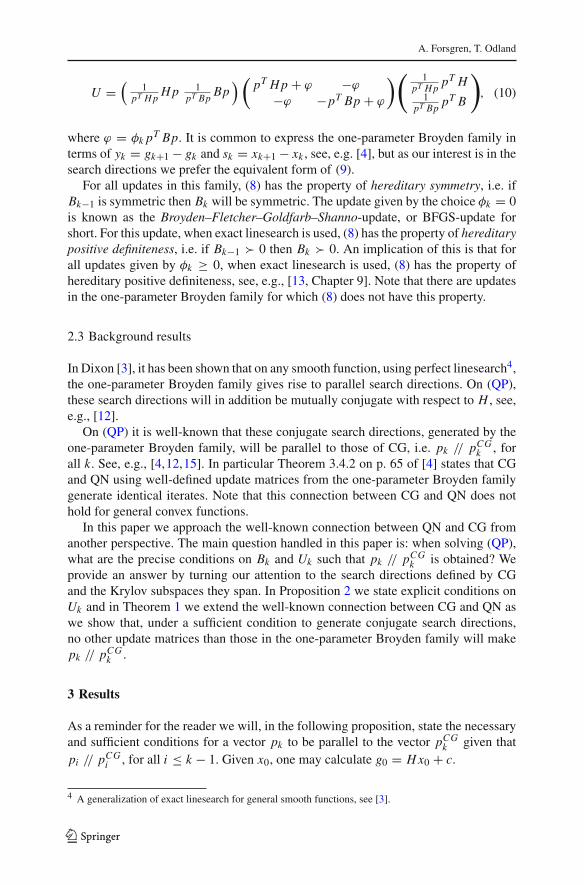
U =(

1pT H p

H p 1pT Bp

Bp) (

pT H p + ϕ −ϕ

−ϕ −pT Bp + ϕ

) (1

pT H ppT H

1pT Bp

pT B

), (10)

where ϕ = φk pT Bp. It is common to express the one-parameter Broyden family interms of yk = gk+1 − gk and sk = xk+1 − xk , see, e.g. [4], but as our interest is in thesearch directions we prefer the equivalent form of (9).

For all updates in this family, (8) has the property of hereditary symmetry, i.e. ifBk−1 is symmetric then Bk will be symmetric. The update given by the choice φk = 0is known as the Broyden–Fletcher–Goldfarb–Shanno-update, or BFGS-update forshort. For this update, when exact linesearch is used, (8) has the property of hereditarypositive definiteness, i.e. if Bk−1 � 0 then Bk � 0. An implication of this is that forall updates given by φk ≥ 0, when exact linesearch is used, (8) has the property ofhereditary positive definiteness, see, e.g., [13, Chapter 9]. Note that there are updatesin the one-parameter Broyden family for which (8) does not have this property.

2.3 Background results

In Dixon [3], it has been shown that on any smooth function, using perfect linesearch4,the one-parameter Broyden family gives rise to parallel search directions. On (QP),these search directions will in addition be mutually conjugate with respect to H , see,e.g., [12].

On (QP) it is well-known that these conjugate search directions, generated by theone-parameter Broyden family, will be parallel to those of CG, i.e. pk // pCG

k , forall k. See, e.g., [4,12,15]. In particular Theorem 3.4.2 on p. 65 of [4] states that CGand QN using well-defined update matrices from the one-parameter Broyden familygenerate identical iterates. Note that this connection between CG and QN does nothold for general convex functions.

In this paper we approach the well-known connection between QN and CG fromanother perspective. The main question handled in this paper is: when solving (QP),what are the precise conditions on Bk and Uk such that pk // pCG

k is obtained? Weprovide an answer by turning our attention to the search directions defined by CGand the Krylov subspaces they span. In Proposition 2 we state explicit conditions onUk and in Theorem 1 we extend the well-known connection between CG and QN aswe show that, under a sufficient condition to generate conjugate search directions,no other update matrices than those in the one-parameter Broyden family will makepk // pCG

k .

3 Results

As a reminder for the reader we will, in the following proposition, state the necessaryand sufficient conditions for a vector pk to be parallel to the vector pCG

k given thatpi // pCG

i , for all i ≤ k − 1. Given x0, one may calculate g0 = H x0 + c.

4 A generalization of exact linesearch for general smooth functions, see [3].

123


Proposition 1 Let p0 = pCG0 = −g0 and pi // pCG

i , for all i ≤ k − 1. Assumepk �= 0, then pk // pCG

k if and only if

(i) pk ∈ Kk+1(p0, H), and,(ii) pT

k H pi = 0, ∀i ≤ k − 1.

Proof For the sake of completeness we include the proof.Necessary: Suppose pk is parallel to pCG

k . Then pk = δk pCGk , for an arbitrary

nonzero scalar δk . As pCGk satisfies (i), it holds that

pk = δk pCGk ∈ Kk+1

(p0, H

),

since Kk+1(p0, H) is a linear subspace. And as pCGk satisfies (ii), it follows that,

pTk H pi = δkδi

(pCG

k

)TH pCG

i = 0, ∀i ≤ k − 1.

Sufficient: Suppose pk satisfies (i) and (ii). The set of vectors {pCG0 , . . . , pCG

k }form an H -orthogonal basis for the space Kk+1(p0, H) and the set of vectors{p0, . . . , pk−1} form an H -orthogonal basis for the space Kk(p0, H). Since pk satis-fies (i) and (ii) it must hold that pk // pCG

k . ��These necessary and sufficient conditions will serve as a foundation for the rest

of our results. We will determine conditions, first on Bk , and second on Uk used initeration k of QN, in order for pk // pCG

k .Given the current iterate xk , one may calculate gk = H xk + c. Hence, in iteration

k of QN, pk is determined from (7) and depends entirely on the choice of Bk . Wemake the assumption that (7) is compatible, i.e. that a solution exists. A well-knownsufficient condition for pk to satisfy (ii) of Proposition 1 is for Bk to satisfy

Bk pi = H pi , ∀i ≤ k − 1. (11)

This condition, known as the hereditary condition, will be used in the following results,which implies that the stated conditions on Bk and later Uk will be sufficient conditions,and not necessary and sufficient as those in Proposition 1. All Bk satisfying (11) canbe seen as defining different conjugate direction methods, but only certain choices ofBk will generate conjugate directions parallel to those of CG.

Assume that Bk is constructed as,

Bk = I + Vk, (12)

i.e. an identity matrix plus a matrix Vk .5 We make no assumptions on Vk exceptsymmetry.

Let B0 = I , then p0 = pCG0 = −g0. Given pi // pCG

i , for all i ≤ k − 1, thefollowing lemma gives sufficient conditions on Bk in order for pk // pCG

k .

5 Any symmetric matrix can be expressed like this.

123


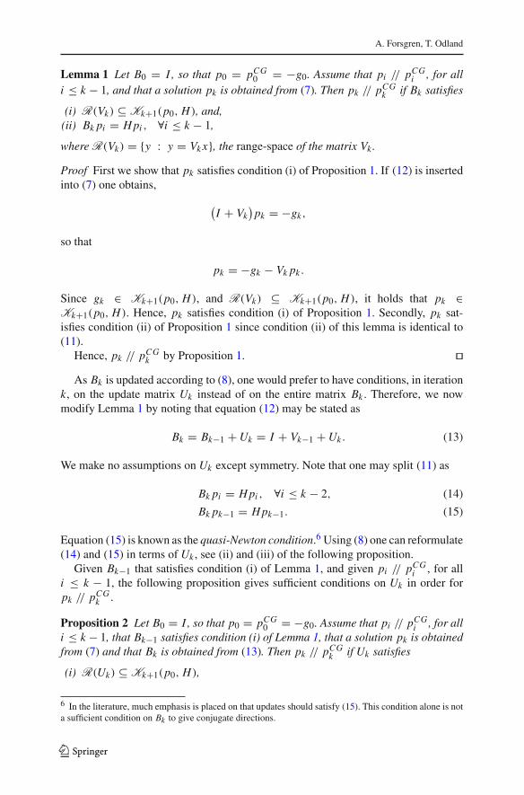
Lemma 1 Let B0 = I , so that p0 = pCG0 = −g0. Assume that pi // pCG

i , for alli ≤ k − 1, and that a solution pk is obtained from (7). Then pk // pCG

k if Bk satisfies

(i) R(Vk) ⊆ Kk+1(p0, H), and,(ii) Bk pi = H pi , ∀i ≤ k − 1,

where R(Vk) = {y : y = Vk x}, the range-space of the matrix Vk.

Proof First we show that pk satisfies condition (i) of Proposition 1. If (12) is insertedinto (7) one obtains,

(I + Vk

)pk = −gk,

so that

pk = −gk − Vk pk .

Since gk ∈ Kk+1(p0, H), and R(Vk) ⊆ Kk+1(p0, H), it holds that pk ∈Kk+1(p0, H). Hence, pk satisfies condition (i) of Proposition 1. Secondly, pk sat-isfies condition (ii) of Proposition 1 since condition (ii) of this lemma is identical to(11).

Hence, pk // pCGk by Proposition 1. ��

As Bk is updated according to (8), one would prefer to have conditions, in iterationk, on the update matrix Uk instead of on the entire matrix Bk . Therefore, we nowmodify Lemma 1 by noting that equation (12) may be stated as

Bk = Bk−1 + Uk = I + Vk−1 + Uk . (13)

We make no assumptions on Uk except symmetry. Note that one may split (11) as

Bk pi = H pi , ∀i ≤ k − 2, (14)

Bk pk−1 = H pk−1. (15)

Equation (15) is known as the quasi-Newton condition.6 Using (8) one can reformulate(14) and (15) in terms of Uk , see (ii) and (iii) of the following proposition.

Given Bk−1 that satisfies condition (i) of Lemma 1, and given pi // pCGi , for all

i ≤ k − 1, the following proposition gives sufficient conditions on Uk in order forpk // pCG

k .

Proposition 2 Let B0 = I , so that p0 = pCG0 = −g0. Assume that pi // pCG

i , for alli ≤ k − 1, that Bk−1 satisfies condition (i) of Lemma 1, that a solution pk is obtainedfrom (7) and that Bk is obtained from (13). Then pk // pCG

k if Uk satisfies

(i) R(Uk) ⊆ Kk+1(p0, H),

6 In the literature, much emphasis is placed on that updates should satisfy (15). This condition alone is nota sufficient condition on Bk to give conjugate directions.

123


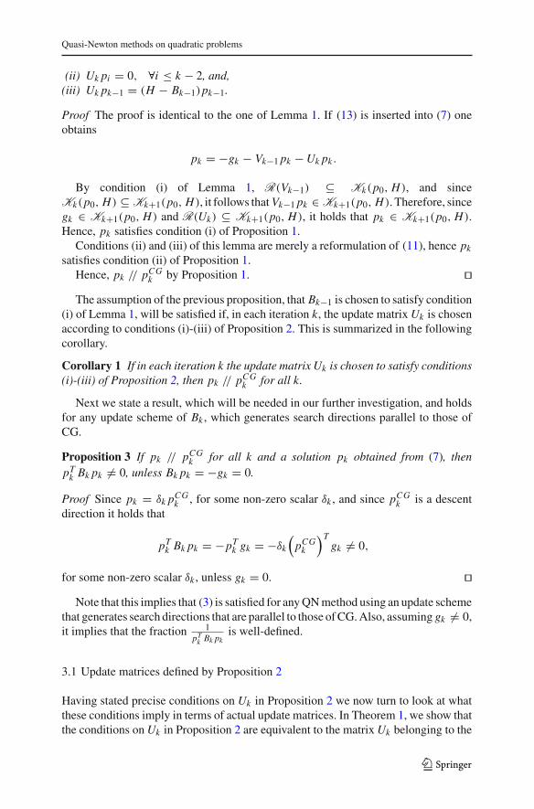
(ii) Uk pi = 0, ∀i ≤ k − 2, and,(iii) Uk pk−1 = (H − Bk−1)pk−1.

Proof The proof is identical to the one of Lemma 1. If (13) is inserted into (7) oneobtains

pk = −gk − Vk−1 pk − Uk pk .

By condition (i) of Lemma 1, R(Vk−1) ⊆ Kk(p0, H), and sinceKk(p0, H) ⊆ Kk+1(p0, H), it follows that Vk−1 pk ∈ Kk+1(p0, H). Therefore, sincegk ∈ Kk+1(p0, H) and R(Uk) ⊆ Kk+1(p0, H), it holds that pk ∈ Kk+1(p0, H).Hence, pk satisfies condition (i) of Proposition 1.

Conditions (ii) and (iii) of this lemma are merely a reformulation of (11), hence pk

satisfies condition (ii) of Proposition 1.Hence, pk // pCG

k by Proposition 1. ��The assumption of the previous proposition, that Bk−1 is chosen to satisfy condition

(i) of Lemma 1, will be satisfied if, in each iteration k, the update matrix Uk is chosenaccording to conditions (i)-(iii) of Proposition 2. This is summarized in the followingcorollary.

Corollary 1 If in each iteration k the update matrix Uk is chosen to satisfy conditions(i)-(iii) of Proposition 2, then pk // pCG

k for all k.

Next we state a result, which will be needed in our further investigation, and holdsfor any update scheme of Bk , which generates search directions parallel to those ofCG.

Proposition 3 If pk // pCGk for all k and a solution pk obtained from (7), then

pTk Bk pk �= 0, unless Bk pk = −gk = 0.

Proof Since pk = δk pCGk , for some non-zero scalar δk , and since pCG

k is a descentdirection it holds that

pTk Bk pk = −pT

k gk = −δk

(pCG

k

)Tgk �= 0,

for some non-zero scalar δk , unless gk = 0. ��Note that this implies that (3) is satisfied for any QN method using an update scheme

that generates search directions that are parallel to those of CG. Also, assuming gk �= 0,it implies that the fraction 1

pTk Bk pk

is well-defined.

3.1 Update matrices defined by Proposition 2

Having stated precise conditions on Uk in Proposition 2 we now turn to look at whatthese conditions imply in terms of actual update matrices. In Theorem 1, we show thatthe conditions on Uk in Proposition 2 are equivalent to the matrix Uk belonging to the

123


one-parameter Broyden family, (10). This implies that, under the sufficient condition(11), there are no other update matrices, even of higher rank, that make pk // pCG

k .The if-direction of Theorem 1, the fact that the one-parameter Broyden family satis-

fies the conditions of Proposition 2 is straightforward. However, the only if-directionsshows that there are no update matrices outside this family that satisfy the conditionsof Proposition 2.

Theorem 1 Assume gk �= 0. A matrix Uk satisfies (i)-(iii) of Proposition 2 if and onlyif Uk can be expressed according to (10), the one-parameter Broyden family, for someφk .

Proof Note that since Kk−1(p0, H) = span{p0, . . . , pk−2}, condition (ii) of Propo-sition 2 can be stated as

Kk−1

(p0, H

)⊆ N

(Uk

),

where N (Uk) = {x : Uk x = 0}, the null-space of Uk . This implies thatdim(N (Uk)) ≥ k−1. Since Uk is symmetric and applying condition (i) of Proposition2 it follows that

R(

Uk

)⊆ Kk−1

(p0, H

)⊥ ∩ Kk+1

(p0, H

)= span

{gk−1, gk

},

and that dim(R(U Tk )) = dim(R(Uk)) ≤ 2.

Hence, one may write a general Uk that satisfies the conditions (i) and (ii) ofProposition 2 as

Uk = (gk−1 gk

) (m1,1 m1,2m1,2 m2,2

)(gT

k−1gT

k

). (16)

Note that due to the linear relationship between {Bk−1 pk−1, H pk−1} and {gk−1, gk}it holds that

gk−1 = −Bk−1 pk−1, gk = αk−1 H pk−1 + gk−1.

Hence, since αk−1 = (pTk−1 Bk−1 pk−1)/(pT

k−1 H pk−1) by the exact linesearch, drop-ping all ′k − 1′-subscripts and letting gk be represented by g+, we obtain

(gT

gT+

)= pT Bp

(0 −11 −1

) (1

pT H ppT H

1pT Bp

pT B

). (17)

We may therefore rewrite (16) as

Uk =(

1pT H p

H p 1pT Bp

Bp) (

m̂1,1 m̂1,2m̂1,2 m̂2,2

)(1

pT H ppT H

1pT Bp

pT B

). (18)

123


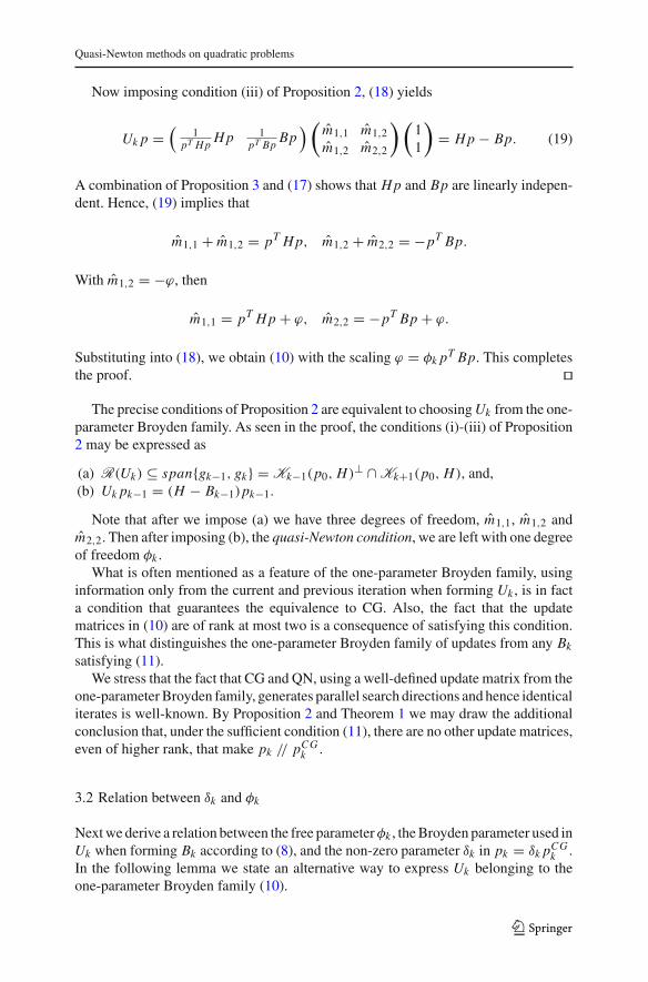
Now imposing condition (iii) of Proposition 2, (18) yields

Uk p =(

1pT H p

H p 1pT Bp

Bp)(

m̂1,1 m̂1,2m̂1,2 m̂2,2

) (11

)= H p − Bp. (19)

A combination of Proposition 3 and (17) shows that H p and Bp are linearly indepen-dent. Hence, (19) implies that

m̂1,1 + m̂1,2 = pT H p, m̂1,2 + m̂2,2 = −pT Bp.

With m̂1,2 = −ϕ, then

m̂1,1 = pT H p + ϕ, m̂2,2 = −pT Bp + ϕ.

Substituting into (18), we obtain (10) with the scaling ϕ = φk pT Bp. This completesthe proof. ��

The precise conditions of Proposition 2 are equivalent to choosing Uk from the one-parameter Broyden family. As seen in the proof, the conditions (i)-(iii) of Proposition2 may be expressed as

(a) R(Uk) ⊆ span{gk−1, gk} = Kk−1(p0, H)⊥ ∩ Kk+1(p0, H), and,(b) Uk pk−1 = (H − Bk−1)pk−1.

Note that after we impose (a) we have three degrees of freedom, m̂1,1, m̂1,2 andm̂2,2. Then after imposing (b), the quasi-Newton condition, we are left with one degreeof freedom φk .

What is often mentioned as a feature of the one-parameter Broyden family, usinginformation only from the current and previous iteration when forming Uk , is in facta condition that guarantees the equivalence to CG. Also, the fact that the updatematrices in (10) are of rank at most two is a consequence of satisfying this condition.This is what distinguishes the one-parameter Broyden family of updates from any Bk

satisfying (11).We stress that the fact that CG and QN, using a well-defined update matrix from the

one-parameter Broyden family, generates parallel search directions and hence identicaliterates is well-known. By Proposition 2 and Theorem 1 we may draw the additionalconclusion that, under the sufficient condition (11), there are no other update matrices,even of higher rank, that make pk // pCG

k .

3.2 Relation between δk and φk

Next we derive a relation between the free parameter φk , the Broyden parameter used inUk when forming Bk according to (8), and the non-zero parameter δk in pk = δk pCG

k .In the following lemma we state an alternative way to express Uk belonging to theone-parameter Broyden family (10).

123


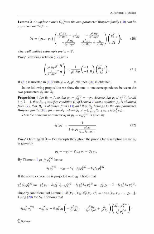
Lemma 2 An update matrix Uk from the one-parameter Broyden family (10) can beexpressed on the form

Uk = (gk−1 gk

)⎛

⎝pT H p

(pT Bp)2 − 1pT Bp

− pT H p(pT Bp)2

− pT H p(pT Bp)2

pT H p(pT Bp)2 + φk

pT Bp

⎞

⎠(

gTk−1

gTk

), (20)

where all omitted subscripts are ′k − 1′.Proof Reversing relation (17) gives

⎛

⎝1

pT H ppT H

1pT Bp

pT B

⎞

⎠ = 1

pT Bp

(−1 1−1 0

)(gT

k−1gT

k

). (21)

If (21) is inserted in (10) with ϕ = φk pT Bp, then (20) is obtained. ��In the following proposition we show the one-to-one correspondence between the

two parameters φk and δk ,

Proposition 4 Let B0 = I , so that p0 = pCG0 = −g0. Assume that pi // pCG

i , for alli ≤ k − 1, that Bk−1 satisfies condition (i) of Lemma 1, that a solution pk is obtainedfrom (7), that Bk is obtained from (13) and that Uk belongs to the one-parameterBroyden family, (10), for some φk , where φk �= −(pT

k−1 Bk−1 pk−1)/(gTk gk).

Then the non-zero parameter δk in pk = δk pCGk is given by

δk(φk) = 1

1 + φkgT

k gk


. (22)

Proof Omitting all ′k − 1′-subscripts throughout the proof. Our assumption is that pk

is given by

pk = −gk − Vk−1 pk − Uk pk .

By Theorem 1 pk // pCGk hence,

δk pCGk =−gk − Vk−1δk pCG

k − Ukδk pCGk .

If the above expression is projected onto gk it holds that

gTk (δk pCG

k )=−gTk gk − δk gT

k Vk−1 pCGk − δk gT

k Uk pCGk = −gT

k gk − 0 − δk gTk Uk pCG

k ,

since by condition (i) of Lemma 1, R(Vk−1)⊆Kk(p0, H) = span{g0, g1, . . . , gk−1}.Using (20) for Uk it follows that

δk gTk pCG

k = −gTk gk − δk gT

k gk

(− pT H p

(pT Bp)2pT H p

(pT Bp)2 + φkpT Bp

)( gTk−1 pCG

k

gTk pCG

k

).

123


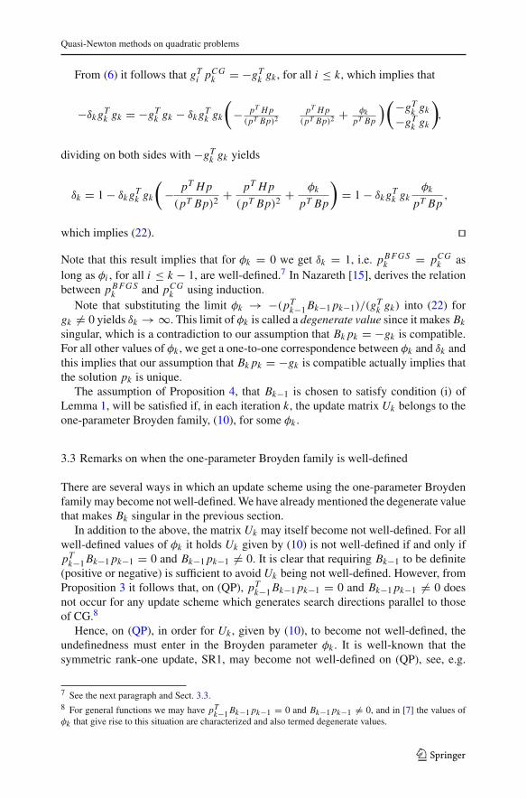
From (6) it follows that gTi pCG

k = −gTk gk , for all i ≤ k, which implies that

−δk gTk gk = −gT

k gk − δk gTk gk

(− pT H p

(pT Bp)2pT H p

(pT Bp)2 + φkpT Bp

)(−gTk gk

−gTk gk

),

dividing on both sides with −gTk gk yields

δk = 1 − δk gTk gk

(− pT H p

(pT Bp)2 + pT H p

(pT Bp)2 + φk

pT Bp

)= 1 − δk gT

k gkφk

pT Bp,

which implies (22). ��Note that this result implies that for φk = 0 we get δk = 1, i.e. pB FGS

k = pCGk as

long as φi , for all i ≤ k − 1, are well-defined.7 In Nazareth [15], derives the relationbetween pB FGS

k and pCGk using induction.

Note that substituting the limit φk → −(pTk−1 Bk−1 pk−1)/(gT

k gk) into (22) forgk �= 0 yields δk → ∞. This limit of φk is called a degenerate value since it makes Bk

singular, which is a contradiction to our assumption that Bk pk = −gk is compatible.For all other values of φk , we get a one-to-one correspondence between φk and δk andthis implies that our assumption that Bk pk = −gk is compatible actually implies thatthe solution pk is unique.

The assumption of Proposition 4, that Bk−1 is chosen to satisfy condition (i) ofLemma 1, will be satisfied if, in each iteration k, the update matrix Uk belongs to theone-parameter Broyden family, (10), for some φk .

3.3 Remarks on when the one-parameter Broyden family is well-defined

There are several ways in which an update scheme using the one-parameter Broydenfamily may become not well-defined. We have already mentioned the degenerate valuethat makes Bk singular in the previous section.

In addition to the above, the matrix Uk may itself become not well-defined. For allwell-defined values of φk it holds Uk given by (10) is not well-defined if and only ifpT

k−1 Bk−1 pk−1 = 0 and Bk−1 pk−1 �= 0. It is clear that requiring Bk−1 to be definite(positive or negative) is sufficient to avoid Uk being not well-defined. However, fromProposition 3 it follows that, on (QP), pT

k−1 Bk−1 pk−1 = 0 and Bk−1 pk−1 �= 0 doesnot occur for any update scheme which generates search directions parallel to thoseof CG.8

Hence, on (QP), in order for Uk , given by (10), to become not well-defined, theundefinedness must enter in the Broyden parameter φk . It is well-known that thesymmetric rank-one update, SR1, may become not well-defined on (QP), see, e.g.

7 See the next paragraph and Sect. 3.3.8 For general functions we may have pT

k−1 Bk−1 pk−1 = 0 and Bk−1 pk−1 �= 0, and in [7] the values ofφk that give rise to this situation are characterized and also termed degenerate values.

123


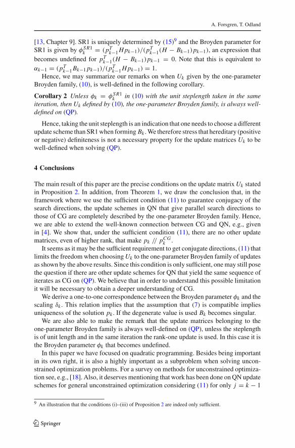
[13, Chapter 9]. SR1 is uniquely determined by (15)9 and the Broyden parameter forSR1 is given by φS R1

k = (pTk−1 H pk−1)/(pT

k−1(H − Bk−1)pk−1), an expression thatbecomes undefined for pT

k−1(H − Bk−1)pk−1 = 0. Note that this is equivalent toαk−1 = (pT

k−1 Bk−1 pk−1)/(pTk−1 H pk−1) = 1.

Hence, we may summarize our remarks on when Uk given by the one-parameterBroyden family, (10), is well-defined in the following corollary.

Corollary 2 Unless φk = φS R1k in (10) with the unit steplength taken in the same

iteration, then Uk defined by (10), the one-parameter Broyden family, is always well-defined on (QP).

Hence, taking the unit steplength is an indication that one needs to choose a differentupdate scheme than SR1 when forming Bk . We therefore stress that hereditary (positiveor negative) definiteness is not a necessary property for the update matrices Uk to bewell-defined when solving (QP).

4 Conclusions

The main result of this paper are the precise conditions on the update matrix Uk statedin Proposition 2. In addition, from Theorem 1, we draw the conclusion that, in theframework where we use the sufficient condition (11) to guarantee conjugacy of thesearch directions, the update schemes in QN that give parallel search directions tothose of CG are completely described by the one-parameter Broyden family. Hence,we are able to extend the well-known connection between CG and QN, e.g., givenin [4]. We show that, under the sufficient condition (11), there are no other updatematrices, even of higher rank, that make pk // pCG

k .It seems as it may be the sufficient requirement to get conjugate directions, (11) that

limits the freedom when choosing Uk to the one-parameter Broyden family of updatesas shown by the above results. Since this condition is only sufficient, one may still posethe question if there are other update schemes for QN that yield the same sequence ofiterates as CG on (QP). We believe that in order to understand this possible limitationit will be necessary to obtain a deeper understanding of CG.

We derive a one-to-one correspondence between the Broyden parameter φk and thescaling δk . This relation implies that the assumption that (7) is compatible impliesuniqueness of the solution pk . If the degenerate value is used Bk becomes singular.

We are also able to make the remark that the update matrices belonging to theone-parameter Broyden family is always well-defined on (QP), unless the steplengthis of unit length and in the same iteration the rank-one update is used. In this case it isthe Broyden parameter φk that becomes undefined.

In this paper we have focused on quadratic programming. Besides being importantin its own right, it is also a highly important as a subproblem when solving uncon-strained optimization problems. For a survey on methods for unconstrained optimiza-tion see, e.g., [18]. Also, it deserves mentioning that work has been done on QN updateschemes for general unconstrained optimization considering (11) for only j = k − 1

9 An illustration that the conditions (i)–(iii) of Proposition 2 are indeed only sufficient.

123


and j = k − 2, deriving an update scheme that satisfies the quasi-Newton conditionand has a minimum violation of it for the previous step, see [14,16].

A further motivation for this research in this paper is that the deeper understandingof what is important in the choice of Uk could be implemented in a limited-memoryQN method. I.e., can one choose which columns to save based on some other criteriathan just picking the most recent ones? See, e.g., [17, Chapter 9], for an introductionto limited-memory QN methods.

Finally, it should be pointed out that the discussion of this paper is limited toexact arithmetic. Even in cases where CG and QN generate identical iterates in exactarithmetic, the difference between numerically computed iterates by the two methodsmay be quite large, see, e.g. [10].

Acknowledgments We thank the referees and the associate editor for their insightful comments andsuggestions which significantly improved the presentation of this paper. Research supported by the SwedishResearch Council (VR).

References

1. Broyden, C.G.: Quasi–Newton methods and their application to function minimisation. Math. Comp.21, 368–381 (1967)

2. Davidon, W.C.: Variable metric method for minimization. SIAM J. Optim. 1(1), 1–17 (1991)3. Dixon, L.C.W.: Quasi–Newton algorithms generate identical points. Math. Program. 2, 383–387 (1972)4. Fletcher, R.: Practical Methods of Optimization, 2nd edn. A Wiley-Interscience. John Wiley & Sons

Ltd., Chichester (1987)5. Fletcher, R., Powell, M.J.D.: A rapidly convergent descent method for minimization. Comput. J. 6(2),

163–168 (1963/1964)6. Fletcher, R., Reeves, C.M.: Function minimization by conjugate gradients. Comput. J. 7, 149–154

(1964)7. Fletcher, R., Sinclair, J.W.: Degenerate values for Broyden methods. J. Optim. Theory Appl. 33(3),

311–324 (1981)8. Gill, P.E., Murray, W., Wright, M.H.: Practical Optimization. Academic Press Inc. Harcourt Brace

Jovanovich, London (1981)9. Gutknecht, M.H.: A brief introduction to Krylov space methods for solving linear systems. In Fron-

tiers of Computational Science, Springer-Verlag, Berlin, pp. 53–62 (2007). In: Proceedings of theInternational Symposium on Frontiers of Computational Science, Nagoya Univ, Nagoya, Dec 12–13,2005.

10. Hager, W.W., Zhang, H.: The limited memory conjugate gradient method. SIAM J. Optim. 23(4),2150–2168 (2013)

11. Hestenes, M.R., Stiefel, E.: Methods of conjugate gradients for solving linear systems. J. Res. Nat.Bur. Stand. 49(1952), 409–436 (1953)

12. Huang, H.Y.: Unified approach to quadratically convergent algorithms for function minimization. J.Optim. Theory Appl. 5, 405–423 (1970)

13. Luenberger, D.G.: Linear and Nonlinear Programming, 2nd edn. Addison-Wesley, Boston, MA (1984)14. Mifflin, R.B., Nazareth, J.L.: The least prior deviation Quasi–Newton update. Math. Programming Ser.

A 65(3), 247–261 (1994)15. Nazareth, L.: A relationship between the BFGS and conjugate gradient algorithms and its implications

for new algorithms. SIAM J. Numer. Anal. 16(5), 794–800 (1979)16. Nazareth, L.: An alternative variational principle for variable metric updating. Math. Program. 30(1),

99–104 (1984)17. Nocedal, J., Wright, S.J.: Numerical Optimization. Springer Series in Operations Research. Springer-

Verlag, New York (1999)18. Powell, M.J.D.: Recent advances in unconstrained optimization. Math. Program. 1(1), 26–57 (1971)

123


19. Saad, Y.: Iterative Methods for Sparse Linear Systems, 2nd edn. Society for Industrial and AppliedMathematics, Philadelphia, PA (2003)

20. Shewchuk, J.R.: An introduction to the conjugate gradient method without the agonizing pain. TechnicalReport, Pittsburgh, PA (1994)

123

On the connection between the conjugate gradient method and quasi-Newton methods on quadratic...

Documents

Transcript of On the connection between the conjugate gradient method and quasi-Newton methods on quadratic...