1

On the Approximate Solution of the

Laminar Boundary-Layer Equations1

Itiro Tani2

Cornell University

Journal of Aeronautical Sciences, vol. 21, pp.487-495, 504, 1954.

Received September 14, 1953.

SUMMARY

A simple method is developed for solving approximately the

equations of the laminar boundary layer. The velocity profile is

assumed as a member of a one-parameter family of curves, the

parameter being different from the usual Pohlhausen parameter.

The Pohlhausen parameter is calculated by a simple quadrature

formula, which is derived from the energy-integral relation. The

relation between the profile parameter and Pohlhausen parameter is

determined from the combination of both momentum-integral and

energy-integral relations. The accuracy of the method is examined

by comparing the results with those of exact solutions for the flow

of incompressible fluid. Satisfactory agreement is obtained. The

method of solution is then extended to the flow of compressible

fluid along a heat-insulated wall, assuming the Prandtl Number

slightly different from unity and the Sutherland formula for the

variation of viscosity with temperature. As an example of the

application, the effect of compressibility on separation point is

discussed.

INTRODUCTION

It has been shown by Stewartson(1) that the momentum

equation for a compressible laminar boundary layer is transformed

into that for an incompressible laminar boundary layer, assuming

that the wall is thermally insulated, that the Prandtl Number is unity,

and that the viscosity is proportional to the absolute temperature. If

any one of the assumptions is dropped, the transformed equation is

no longer of the same form as that for an incompressible flow, but it

is still easy to solve because of the disappearance of variable

1 This research, carried out at the Graduate School of Aeronautical Engineering, Cornell University, was supported by the United States Air Force under Contract No.

AF 33 (038)-21406, monitored by the Office of Scientific Research. Air Research

and Development Command. The writer wishes to take this opportunity to acknowledge helpful discussions with Professors W. R. Sears and Nicholas Rott of

the Cornell University during the course of the work.

2

density. Therefore it seems adequate to consider first the laminar

boundary layer in incompressible fluids.

The most frequently used method of solving the boundary layer

equations approximately is the momentum-integral method, in

which the momentum equation is integrated over the boundary

layer thickness, and is hence satisfied only in average. By assuming

a definite form for the velocity profile as a function of the normal

distance, an ordinary differential equation is obtained, with the

distance along the wall as the independent variable. In the original

method due to von Karman and Pohlhausen(2), fourth-degree

velocity profile is assumed, whose coefficients are determined by

the boundary conditions at the wall as well as at the outer edge of

the boundary layer. Consequently, the velocity profile is expressed

as a member of a one-parameter family of curves, with

dx

du12

νθ

λ =

as the parameter, which makes its appearance through the condition

that the momentum equation should be satisfied at the wall.

This method gives a reasonably accurate solution in a region of

accelerated flow, but its adequacy in a region of retarded flow has

been questioned. Separation of flow may actually occur where the

method fails to give it. Various attempts have been made to increase

the accuracy of the method. For example, Howarth(3) used the

velocity profile obtained from the exact solution for the case when

the velocity outside the boundary layer decreases linearly with the

distance; Schlichting and Ulrich(4) assumed a sixth-degree

polynomial for the velocity profile, so that it could satisfy

additional conditions at the wall as well as at the outer edge of the

boundary layer. These refinements generally yield fairly good

results when compared with the original method due to Pohlhausen.

Strictly speaking, however, none of the methods is sufficiently

accurate because the velocity profile is expressed as a member of

the family of curves with the Pohlhausen parameter λ , whereas

the results of certain exact solutions suggest that λ cannot fix the

velocity profile. In particular, λ should have a certain definite

value at the separation point according to the assumption, but this is

not the case according to the exact solutions, the value λ at

separation depending considerably on the the velocity distribution

2 Professor, University of Tokyo, Japan. On leave from the University of Tokyo.

3

outside the boundary layer(5).

It is reasonable to suppose that the difficulty may be reduced by

using a velocity profile with two parameters, one of which is λ

and the other new. This has actually been done by Wieghardt(6),

who assumed an eleventh-degree velocity profile and determined

the parameters by using the momentum-integral as well as the

energy-integral relations, the latter of which is obtained by

multiplying the momentum equation by velocity and integrating

across the boundary layer thickness. Satisfactory results can be

obtained, but the method appears quite tedious for practical

application. An interesting modification has been proposed by

Walz(7), who used a one-parameter family of curves again but gave

up the fulfillment of the condition that the momentum equation

should hold at the wall. The procedure is thus considerably

simplified, but results of comparatively high accuracy can still be

obtained. Truckenbrodt(8) has recently extended the method so that

the laminar and turbulent boundary layers may be treated along

similar lines.

It is to be pointed out that the improvement of accuracy is

attained by dropping one of the boundary conditions at the wall and

satisfying the energy integral relation instead. Since the Pohlhausen

parameter λ enters only through the boundary condition, this is

equivalent to saying that better results may be obtained by

abandoning λ for use as the profile parameter that should be

determined such that momentum-integral and energy-integral

relations are both satisfied. The conclusion seems to be quite

natural, because λ cannot fix the velocity profile, as mentioned

above.

This method of approach is adopted in the present investigation.

A simple fourth-degree polynomial is used as the velocity profile,

quite the same as the original Pohlhausen scheme, but dropping one

of the boundary conditions at the wall. Consequently, one of the

coefficients of the polynomial remains undetermined, and it is used

as the parameter for the velocity profile. Both the

momentum-integral and energy-integral relations are considered,

from which the relation between the profile parameter and the

distance along the wall is determined. The analysis is given in the

first part of -the paper, and it is shown that satisfactory results are

obtained when compared with the exact solutions.

4

In the second part of the paper, the analysis is extended to the

laminar boundary layer in compressible fluids. The wall is

assumed to be thermally insulated, but the other restrictions

imposed by Stewartson are removed. The Prandtl Number may be

different from unity, but the difference from unity is assumed small.

The so-called Sutherland formula is adopted for the variation of

viscosity with temperature, because it is considered desirable to use

as accurate a formula as possible at high Mach Numbers where the

variations in temperature are considerable. In order to simplify the

analysis, however, a simple relation between temperature and

velocity is assumed, the effect of Prandtl Number being taken into

account approximately. The momentum equation is then

transformed by the method proposed Rott(9), which is a useful

extension of the original Stewartson transformation. The resulting

equation is no longer of the same form as that for the

incompressible flow, but it is still amenable to solution by a similar

technique as mentioned above. The accuracy of the solution is

checked in the case of a flat plate by comparing with Crocco’s

results(10), and it is found to be satisfactory. The method of

solution is then applied for estimating the separation point when the

velocity outside the boundary layer decreases linearly with the

distance.

(I) LAMINAR BOUNDARY LAYER IN INCOMPRESSIBLE

FLUIDS

Basic Equations

Consider first the steady two-dimensional laminar boundary

layer flow of an incompressible fluid. The continuity equation is

0=∂∂

+∂∂

y

v

x

u, (1)

and the momentum equation is

2

21

1y

u

dx

duu

y

uv

x

uu

∂+=

∂∂

+∂∂

ν , (2)

where x and y are the distances measured along and normal to the

wall, respectively, u and v are the velocity components in the

directions x and y, respectively, 1u is the velocity outside the

boundary layer, and ν is the kinematic viscosity. Integrating Eq.

(2) with respect to y from y = 0 to y = δ , where δ is the

5

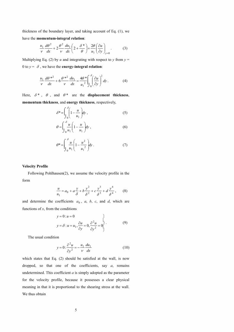
thickness of the boundary layer, and taking account of Eq. (1), we

have the momentum-integral relation:

01

122

1 2*22

=

∂∂

=

++y

y

u

udx

du

dx

du θθδ

νθθ

ν. (3)

Multiplying Eq. (2) by u and integrating with respect to y from y =

0 to y = δ , we have the energy-integral relation:

⌡

⌠

∂∂

=+δ

θν

θθν

0

2

21

122

1 *4*6

*dy

y

u

udx

du

dx

du. (4)

Here, *δ , θ , and *θ are the displacement thickness,

momentum thickness, and energy thickness, respectively,

⌡

⌠

−=

δ

δ0 1

1* dyu

u, (5)

⌡

⌠

−=

δ

θ0 11

1 dyu

u

u

u, (6)

⌡

⌠

−=

δ

θ0

21

2

1

1* dyu

u

u

u. (7)

Velocity Profile

Following Pohlhausen(2), we assume the velocity profile in the

form

4

4

3

3

2

2

01 δδδδ

yd

yc

yb

yaa

u

u++++= , (8)

and determine the coefficients 0a , a, b, c, and d, which are

functions of x, from the conditions

=∂

∂=

∂∂

==

==

0,0,:

0:0

2

2

1y

u

y

uuuy

uy

δ. (9)

The usual condition

dx

duu

y

uy 11

2

2

:0ν

−=∂

∂= (10)

which states that Eq. (2) should be satisfied at the wall, is now

dropped, so that one of the coefficients, say a, remains

undetermined. This coefficient a is simply adopted as the parameter

for the velocity profile, because it possesses a clear physical

meaning in that it is proportional to the shearing stress at the wall.

We thus obtain

6

3

2

2

2

2

1

1386

−+

+−=

δδδδδyy

qyyy

u

u. (11)

Introducing the nondimensional quantities

D=δδ *

, E=δθ

, F=δθ *

, (12)

E

DH ==

θδ *

, E

FG ==

θθ *

, (13)

Py

u

uy

=

∂∂

=01

2θ, Qdy

y

u

u=

⌡

⌠

∂∂

δθ

0

2

21

*4, (14)

we can write Eqs. (3) and (4) in the form

Pdx

duH

dx

du=++ 1

221 )2(2

νθθ

ν, (15)

Qdx

duG

dx

dGu=+ 1

22221 6

νθθ

ν, (16)

where

205

2 aD −= , (17)

25210535

42aa

E −+= , (18)

28605460

23

5005

73

5005

8763

2 aaaF −−+= , (19)

aEP 2= , (20)

)3448(35

4 2aaFQ +−= . (21)

The quantities D, E, F, G, H, P, and Q are functions of a only, and

their numerical values are tabulated in Table 1.

Quadrature Formula for Momentum Thickness

It is readily shown that Eq. (15) may be integrated in the

quadrature formula

∫+−=x

nndxuAu

01

)1(1

2

νθ

, (22)

provided that the distance x is measured from the point where

0=θ , and that λ)23( HP +− can be replaced by a linear

function of λ such that

λλ nAHP −=+− )23( , (23)

where A and n are constants and

7

dx

du12

νθ

λ = (24)

is the so-called Pohlhausen parameter. This method of approximate

integration was put forward independently by Hudimoto(11) and

the present writer(12) early in 1941. The values A = 0.44 and n = 5

proposed by the present writer were obtained by evaluating the left

side of Eq. (23) from Howarth's solution for the case when the

velocity outside the boundary layer decreases linearly with the

distance(3). Formulas of a similar type have also been found by

Young and Winterbottom(13), Walz(14), and Thwaites(15),

independently.

It is not possible, however, to proceed similarly in the present

calculation, because λ is no longer used as the profile parameter.

Instead, Q is a slowly changing function of a, so that it may be

replaced by a constant value mQ . Eq. (16) is then integrated in the

form

∫−=x

m dxuuQG0

51

61

22

νθ

. (25)

Replacing, moreover, the function G by a constant value mG , we

have

∫−=x

m

m dxuuG

Q

0

51

612

2

νθ

. (26)

As will be seen later, Q = 1.079 and G = 1.567 for the flow along a

flat plate. Using these values for mQ and mG , we get

∫−=x

dxuu0

51

61

2

44.0νθ

, (27)

which is exactly the same as previously obtained from the

momentum-integral. It was Truckenbrodt(8) who first found that

the quadrature formula for the momentum thickness may also be

deduced from the energy-integral, although he used the velocity

profile obtained from the exact solution for the case when the

velocity outside the boundary layer is proportional to the power of

distance.

We now consider Eq. (27) as the first approximate solution for

νθ 2

. We then calculate λ by Eq. (24). Therefore, we determine

λ as the function of x. But, since it is a, and not λ , that is used as

the parameter for the velocity profile, it is necessary to obtain a

relation that relates λ and a.

8

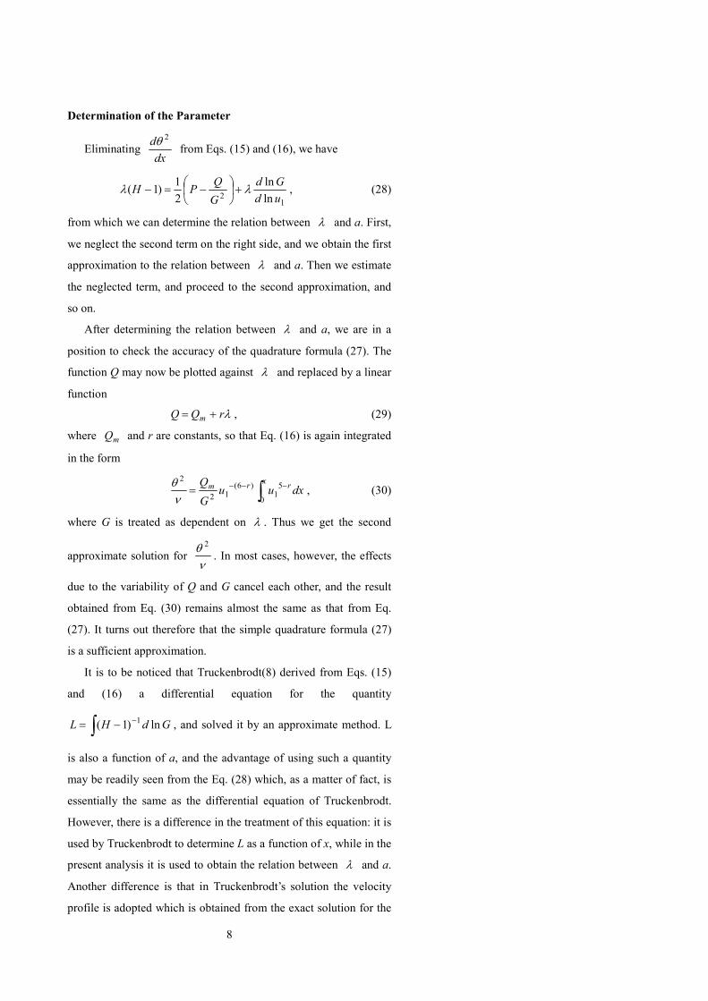
Determination of the Parameter

Eliminating dx

d2θ from Eqs. (15) and (16), we have

1

2 ln

ln

2

1)1(

ud

Gd

G

QPH λλ +

−=− , (28)

from which we can determine the relation between λ and a. First,

we neglect the second term on the right side, and we obtain the first

approximation to the relation between λ and a. Then we estimate

the neglected term, and proceed to the second approximation, and

so on.

After determining the relation between λ and a, we are in a

position to check the accuracy of the quadrature formula (27). The

function Q may now be plotted against λ and replaced by a linear

function

λrQQ m += , (29)

where mQ and r are constants, so that Eq. (16) is again integrated

in the form

∫ −−−=x

rrm dxuuG

Q

0

51

)6(12

2

νθ

, (30)

where G is treated as dependent on λ . Thus we get the second

approximate solution for νθ 2

. In most cases, however, the effects

due to the variability of Q and G cancel each other, and the result

obtained from Eq. (30) remains almost the same as that from Eq.

(27). It turns out therefore that the simple quadrature formula (27)

is a sufficient approximation.

It is to be noticed that Truckenbrodt(8) derived from Eqs. (15)

and (16) a differential equation for the quantity

∫ −−= GdHL ln)1(1

, and solved it by an approximate method. L

is also a function of a, and the advantage of using such a quantity

may be readily seen from the Eq. (28) which, as a matter of fact, is

essentially the same as the differential equation of Truckenbrodt.

However, there is a difference in the treatment of this equation: it is

used by Truckenbrodt to determine L as a function of x, while in the

present analysis it is used to obtain the relation between λ and a.

Another difference is that in Truckenbrodt’s solution the velocity

profile is adopted which is obtained from the exact solution for the

9

special case when the velocity outside the boundary layer is

proportional to the power of the distance, while in the present

analysis the velocity profile is assumed as a simple polynomial,

which is more convenient to be extended to the case of

compressible fluids.

Particular Values of the Parameter

As clearly indicated by Eq. (28), the relation between λ and a

is not universal, but depends on the velocity distribution outside the

boundary layer. However, there are a couple of particular values of

a corresponding to certain definite conditions. For example, the

separation point is characterized by the particular value a = 0.

Other particular cases are the flow along a flat plate and the flow at

the stagnation point.

For the flow along a flat plate, 0=λ and G = constant.3

Therefore we have the condition

2

G

QP = , (31)

from which we obtain

858.1=a (32)

as the particular value of the parameter for the flat plate. We have

also

P = 0.439, Q = 1.079, G = 1.567, H = 2.60, (33)

while the Blasius solution for the flat plate gives

P = 0.441, Q = 1.090, G = 1.572, H = 2.59. (34)

It appears therefore that the present approximate method predicts

the flat plate characteristics with satisfactory accuracy.

In order to find the condition at the stagnation point, we put

01 =u in Eqs. (15) and (16) and eliminate dx

du1 from them. We

then have

2

32 G

Q

H

P=

+ (35)

as the equation for determining the value of a. Unfortunately,

however, it is found that there is no root of the equation in the

physically significant range of a. Similar difficulties have already

been experienced in connection with the refinement of the

3 At the minimum pressure point of a flow with pressure gradient λ vanishes but

G is not necessarily stationary.

10

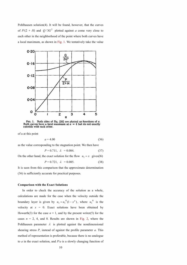
Pohlhausen solution(4). It will be found, however, that the curves

of P/(2 + H) and 23/ GQ plotted against a come very close to

each other in the neighborhood of the point where both curves have

a local maximum, as shown in Fig. 1. We tentatively take the value

of a at this point

a = 4.00 (36)

as the value corresponding to the stagnation point. We then have

P = 0.711, λ = 0.084. (37)

On the other hand, the exact solution for the flow xu =1 gives(l6)

P = 0.721, λ = 0.085. (38)

It is seen from this comparison that the approximate determination

(36) is sufficiently accurate for practical purposes.

Comparison with the Exact Solutions

In order to check the accuracy of the solution as a whole,

calculations are made for the case when the velocity outside the

boundary layer is given by )1(0

11nxuu −= , where

01u is the

velocity at x = 0. Exact solutions have been obtained by

Howarth(3) for the case n = 1, and by the present writer(5) for the

cases n = 2, 4, and 8. Results are shown in Fig. 2, where the

Pohlhausen parameter λ is plotted against the nondimensional

shearing stress P, instead of against the profile parameter a. This

method of representation is preferable, because there is no analogue

to a in the exact solution, and P/a is a slowly changing function of

11

a. It will be seen that the accuracy is satisfactory except for the case

n = 8. Although it is difficult to extend the calculation right up to

the separation point because of the considerable change in the value

of 1ln

ln

ud

Gd, it is still possible to arrive at a point so near to the

separation point that the latter point may be extrapolated with

sufficient accuracy. The result seems to be encouraging, since the

method can predict fairly accurately how the relation between λ

and P (hence λ and a) changes in accordance with the velocity

distribution outside the boundary layer. Such a change was

demonstrated by the present writer(5), but until now there has been

proposed no satisfactory solution which takes this effect into

account.

(II) LAMINAR BOUNDARY LAYER IN COMPRESSIBLE

FLUIDS

Basic Equations

For the steady two-dimensional laminar boundary layer in

compressible fluids, we have the continuity equation

12

0)()( =∂∂

+∂∂

vy

ux

ρρ , (39)

the momentum equation

∂∂

∂∂

+=∂∂

+∂∂

y

u

ydx

duu

y

uv

x

uu µρρρ 1

11 , (40)

and the energy equation

2

111

∂∂

+

∂∂

∂∂

+−=∂∂

+∂∂

y

u

y

Tk

ydx

duuu

y

Tvc

x

Tuc pp µρρρ ,

(41)

where ρ is the density, µ is the viscosity, k is the thermal

conductivity, pc is the specific heat at constant pressure, T is the

absolute temperature, suffix 1 denotes the condition at the outer

edge of the boundary layer, and other symbols have the same

meaning as defined in Part I. µ and k are considered as functions

of T, while pc and the Prandtl Number

k

c pµσ ==Pr (42)

are assumed constant. Since the pressure remains constant across

the boundary layer, we have

T

T1

1

=ρρ

. (43)

Outside the boundary layer We have the isentropic relationship

0

1

1

0

1

T

T=

−γ

ρρ

, (44)

where γ is the ratio of specific heats, and the suffix 0 denotes a

certain reference condition.

It is assumed that there is no heat transfer through the wall.

Therefore we have the condition

0=y : 0=∂∂y

T. (45)

The Prandtl Number σ is assumed to be slightly different from

unity such that the square of the quantity

σξ −= 1 (46)

may be neglected compared to unity. Finally, the viscosity is

assumed to be given by the Sutherland formula

0

0T

TCµµ = , (47)

where

13

ST

ST

T

TC

++

= 0

2/1

0

, (48)

and S is a constant which for air has the value 216°R.

C is not assumed constant, as usually done, but treated as a

function of the temperature, because it seems highly desirable to

use as accurate a. formula as possible for the variation of viscosity

with temperature.

Temperature Profile

For a Prandtl Number of unity and zero heat transfer at the wall,

the analysis can be considerably simplified because the energy

equation (41) is replaced by a simple relation between temperature

and velocity, viz.,

−

−+=

21

2

21

21

1

12

11

u

u

c

u

T

T γ, (49)

where 1c is the local sound speed at the outer edge of the

boundary layer. Assuming the Prandtl Number slightly different

from unity, we write

+

−

−+= Φξσ

γ2

1

2

21

21

1

12

11

u

u

c

u

T

T, (50)

where Φ is an undetermined function of 1u

u such that 0=Φ

when 01

=u

u. This approximate expression is exact when 1=σ ,

and, moreover, it gives the temperature at the wall

−+=

21

21

12

11

c

uTTwall

γσ , (51)

which seems to be supported by the results of calculation due to

Tifford and Chu(17) even in the presence of a pressure gradient.

Assuming the temperature boundary layer has the same

thickness as the velocity boundary layer,4 and integrating Eq. (41)

with respect to y from y = 0 to δ=y , we have

∫∫ −=−δδρρ

0

221

01 )(

2

1)( dyuuudyTTuc p . (52)

Substituting Eq. (50) we obtain

∫∫

−=

δδρΦρ

0 21

2

01 dyu

uudyu , (53)

4 See also the subsequent footnote.

14

which yields an integral condition to be satisfied by the function

Φ .

Stewartson-Rott Transformation

It was shown by Stewartson(1) that the momentum equation

(40) may be transformed into that for an incompressible fluid,

provided that there is no heat transfer, the Prandtl Number is unity,

and the viscosity is proportional to the absolute temperature. The

transformation was modified by Rott(9) such that the effect of

Prandtl Number is taken into account, by assuming the temperature

profile in a form similar to Eq. (50) where the term Φξ is omitted.

The transformation is given by

⌡⌠

=

⌡

⌠

=

+−

y

x

dyT

TY

dxT

TX

0 0

)2/1(

0

1

0

)2/1()1/(

0

1

ρρ

σ

σγγ

, (54)

where x and y are the coordinates of the original flow, and X and Y

are the coordinates of the transformed flow.

Applying the transformation (54) to the momentum equation

(40), and making use of the temperature profile (50) we obtain

∂∂

∂∂

++=∂∂

+∂∂

Y

UC

YdX

dUUB

Y

UV

X

UU 0

11)1( νΦξ

(55)

where U and V are the velocity components in the directions X and

Y, 1U is the velocity outside the boundary layer in the

transformed flow, and

21

21

21

21

2

11

2

1

c

u

c

u

B−

+

−

=γσ

γ

. (56)

There exists a relation between 1U and 1u such that

1

)2/1(

1

01 u

T

TU

σ

= , (57)

and, moreover

11 u

u

U

U= . (58)

Eq. (55) is no longer of the same form as Eq. (2) for the

15

incompressible flow, because the restrictions imposed on the

Prandtl Number and the viscosity-temperature relation have been

removed. It is still easy to solve, however, since the variable

density has disappeared.

Integrating (55) with respect to Y from Y = 0 to Y = ∆ , where

∆ is the thickness of the boundary layer in the transformed flow,

we have

010

1

0

22

0

1 2*22

=

∂∂

=

+++ ∫YY

U

UdY

B

dX

dU

dX

dU ΘΦ

Θξ

Θ∆

νΘΘ

ν

∆.

(59)

Multiplying Eq. (55) by U and integrating with respect to Y from Y

= 0 to Y = ∆ , we have

∫∫

∂∂

=

++

∆∆ ΘΦ

Θξ

νΘΘ

ν 0

2

21

0 1

1

0

22

0

1 *4

*3

21

*6

*dY

Y

UC

UdY

U

UB

dX

dU

dX

dU

(60)

These equations are the analogues of the momentum-integral

relation (3) and energy-integral relation (4), respectively, and *∆ ,

Θ , and *Θ are the displacement thickness, momentum thickness,

and energy thickness in the transformed flow, respectively:

⌡

⌠

−=

∆

∆0 1

1* dYU

U, (61)

⌡

⌠

−=

∆

Θ0 11

1 dYU

U

U

U, (62)

⌡

⌠

−=

∆

Θ0

21

2

1

1* dYU

U

U

U. (63)

Velocity Profile

We now assume the velocity profile in the form

3

2

2

2

2

1

1386

−+

+−=

∆∆∆∆∆YY

aYYY

U

U, (64)

where a is the profile parameter. This is exactly the same as used in

incompressible flow, Eq. (11).

Since C and Φ are functions of 1u

u, or of

1U

U by virtue of

Eq. (58), they may be considered as functions of ∆Y. We assume

therefore

16

3

3

32

2

210∆

α∆

α∆

αα YYYC +++= , (65)

4

4

43

3

32

2

210∆

β∆

β∆

β∆

ββΦ YYYY++++= , (66)

where the coefficients, s'α and s'β , are determined by the

conditions5

Y = 0: 0CC = , 0=∂∂Y

C, 0=Φ , 0=

∂∂Y

Φ,

Y = ∆ : 1CC = , 0=∂∂Y

C, 0=Φ , 0=

∂∂Y

Φ, (67)

and

*0 1

ΘΦ∆

=⌡⌠

dYU

U, (68)

the last condition being obtained from Eqs. (53) and (63).

The reference condition 0 is now chosen such that the

temperature 0T is given by the relation

−

+=2

1

21

102

11

c

uTT

γσ . (69)

In other words, 0T is equal to the wall temperature [Eq. (51)].

With this definition we have

10 =C ,

ST

ST

T

TC

++

=

1

0

2/1

0

11 . (70)

Eqs. (59) and (60) are then written in the form

PdX

dUBKH

dX

dU=+++ 1

0

22

0

1 )2(2νΘ

ξΘ

ν, (71)

)]1(1[3

216 1

1

0

2222

0

1 −+=

++ CJQdX

dUGB

dX

dGU

νΘ

ξΘ

ν,

(72)

respectively, where G, H, P, and Q are given by Eqs. (13), (17),

(18), (19), (20), and (21), and

−−= 2

3127410

19763

57915

146

2145

5841aa

EK , (73)

5 These boundary conditions are based on the assumption that the temperature

boundary layer has the same thickness as the velocity boundary layer. This is not

correct except when the Prandtl Number is unity. However, the error due to this

assumption is considered small, because the function C is multiplied by 2

∂∂Y

U

which is small near the outer edge of the boundary layer, and also the function Φ

is multiplied by ξ which is assumed small in the present analysis.

17

+−= 2

84

1

105

13

35

161aa

QJ . (74)

K and J are also dependent only on a, and their numerical values

are given in Table 1.

Eqs. (71) and (72) are almost identical with Eqs. (15) and (16)

for incompressible flow, the only difference being in the term

proportional to Bξ and the term proportional to ( 11 −C ). These

additional terms represent the effect of Prandtl Number different

from unity, and the effect of viscosity-temperature relation different

from a simple proportionality, respectively.

Approximate Method of Solution

Eqs. (71) and (72) may be solved in exactly the same way as in

incompressible flow. The quadrature formula for the momentum

thickness in the transformed flow is

∫ −+= − X

m

m

m dXCJUUG

Q

01

51

612

0

2

)]1(1[νΘ

, (75)

which is obtained from Eq. (72) by neglecting the term Bξ3

2 and

replacing Q, G, and J by constant values corresponding to the flow

along a flat plate.6 Then, eliminating

dX

d2Θ from Eqs. (71) and

(72), we obtain

112 ln

ln)]1(1[

22

1)]2(1[

Ud

GdCJ

G

QPKBH ΛξΛ +−+−=−+− ,

(76)

which yields the relation between the profile parameter a and the

Pohlhausen parameter in the transformed flow

dX

dU1

0

2

νΘ

Λ = . (77)

Eqs. (75), (76), and (77) correspond to Eqs. (26), (28), and (24),

respectively.

Skin Friction on a Flat Plate

In order to check the accuracy of the method, the skin friction

on a flat plate is calculated and compared with that given by other

solutions. First, the parameter a is determined from the condition

6 For most practical purposes, values corresponding to incompressible flow (a =

1.857, 44.0/2 =mm GQ , 184.0=mJ ) may be used with sufficient accuracy.

18

)]1(1[ 12−+= CJ

G

QP , (78)

which is obtained by putting 0=Λ and G = constant in Eq. (76).

Next, the momentum thickness Θ in the transformed flow is

determined by integrating Eq. (71) in the form

1

02

U

XPν

Θ = . (79)

Then the, coefficient of skin friction based on the free-stream

characteristics is given by

Re

24

102

11 C

P

y

u

uC

y

f =

∂∂

==

µρ

, (80)

where 1

1Reνxu

= is the Reynolds Number based on the distance

from the leading edge.

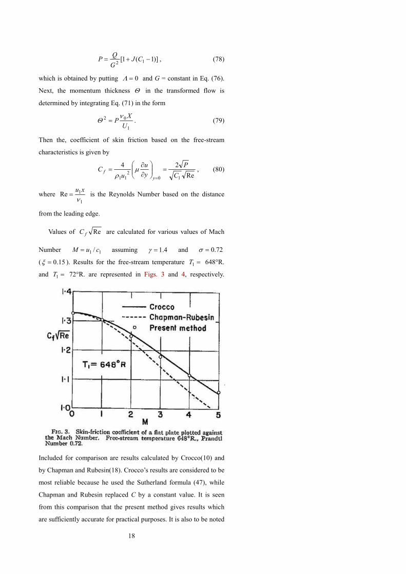
Values of RefC are calculated for various values of Mach

Number 11 / cuM = assuming 4.1=γ and 72.0=σ

( 15.0=ξ ). Results for the free-stream temperature =1T 648°R.

and =1T 72°R. are represented in Figs. 3 and 4, respectively.

Included for comparison are results calculated by Crocco(10) and

by Chapman and Rubesin(18). Crocco’s results are considered to be

most reliable because he used the Sutherland formula (47), while

Chapman and Rubesin replaced C by a constant value. It is seen

from this comparison that the present method gives results which

are sufficiently accurate for practical purposes. It is also to be noted

19

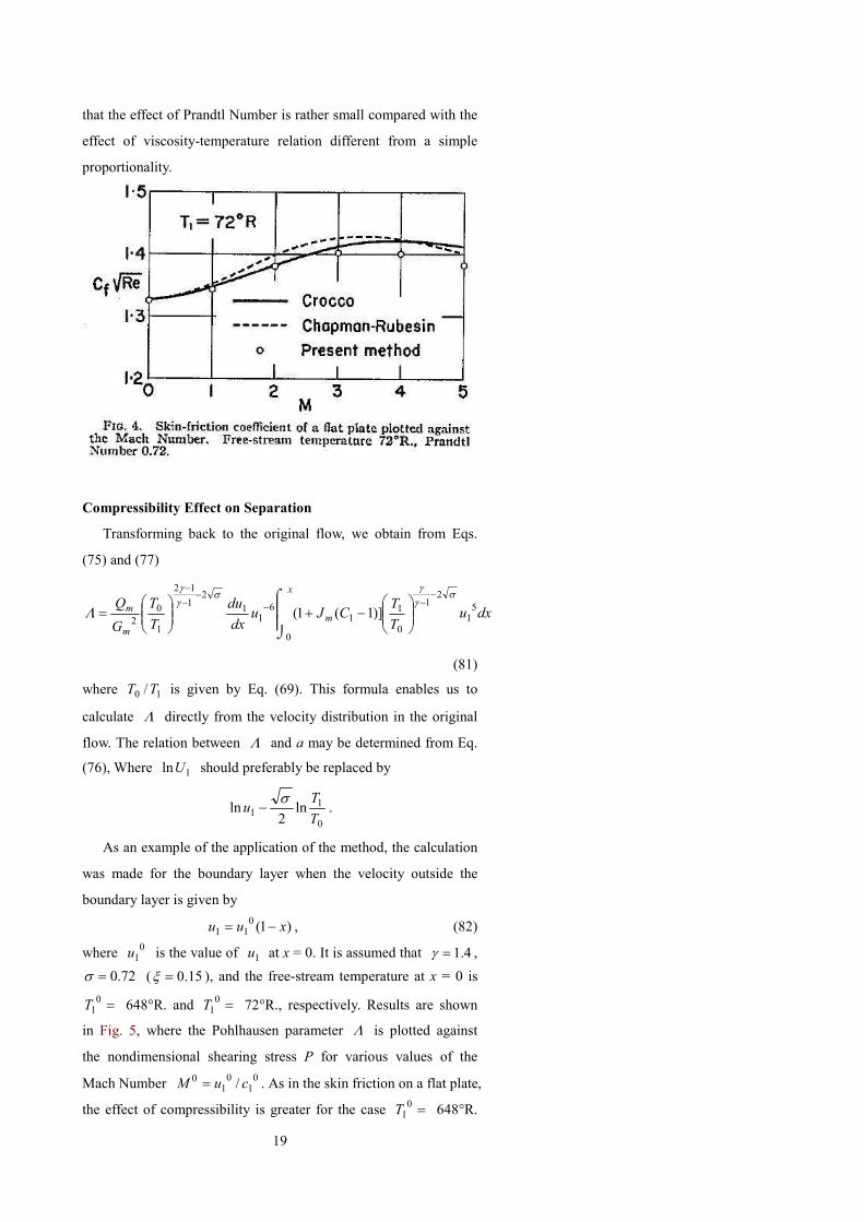
that the effect of Prandtl Number is rather small compared with the

effect of viscosity-temperature relation different from a simple

proportionality.

Compressibility Effect on Separation

Transforming back to the original flow, we obtain from Eqs.

(75) and (77)

⌡

⌠

−+

=

−−−

−−− x

m

m

m dxuT

TCJu

dx

du

T

T

G

Q

0

51

21

0

11

61

1

21

12

1

0

2)]1(1(

σγγ

σγγ

Λ

(81)

where 10 /TT is given by Eq. (69). This formula enables us to

calculate Λ directly from the velocity distribution in the original

flow. The relation between Λ and a may be determined from Eq.

(76), Where 1lnU should preferably be replaced by

0

11 ln

2ln

T

Tu

σ− .

As an example of the application of the method, the calculation

was made for the boundary layer when the velocity outside the

boundary layer is given by

)1(0

11 xuu −= , (82)

where 0

1u is the value of 1u at x = 0. It is assumed that 4.1=γ ,

72.0=σ ( 15.0=ξ ), and the free-stream temperature at x = 0 is

=01T 648°R. and =0

1T 72°R., respectively. Results are shown

in Fig. 5, where the Pohlhausen parameter Λ is plotted against

the nondimensional shearing stress P for various values of the

Mach Number 0

10

10 / cuM = . As in the skin friction on a flat plate,

the effect of compressibility is greater for the case =01T 648°R.

20

than for the case =01T 72°R.

The separation point is determined by locating the values of c

for which Λ attains the values corresponding to P = 0. Results of

this calculation are shown in Fig. 6, where the velocity ratio

011 /uu at the separation point is plotted against the Mach Number

0M . Included also is the result calculated by Stewartson(1) by

assuming that the Prandtl Number is unity, the viscosity is

proportional to temperature, and the value of Λ at separation is

21

the same as for incompressible flow. In spite of these assumptions,

Stewartson’s results appear to be comparatively good; this is

because of the fortunate circumstances that the separation is

delayed by the effect of viscosity-temperature relation different

from a simple proportionality, while it is hastened by the effect of

distortion of velocity distribution in the transformation (54) and

(57).

References

1. Stewartson, K., Correlated Incompressible and Compressible

Boundary Layers, Proc. Roy. Soc., London, Vol. 200, pp. 84-100,

1949.

2. Pohlhausen, K., Zur nährungsweisen Integration der

Differentialgleichung der laminaren Granzschicht, Zeitschr. f.

angew. Math. u. Mech., Vol. 1, pp. 252-268, 1921.

3. Howarth, L., On the Solution of the Laminar Boundary Layer

Equations, Proc. Roy. Soc., London, Vol. 164, pp. 547-579, 1938.

4. Schlichting, H., and Ulrich, A., Zur Berechnung des Umschlages

Iaminar-turbulent, Jahrbuch der deutschen Luftfahrtforschung, 18,

pp. 8-36, 1942.

5. Tani, I., On the Solution of the Laminar Boundary Layer

Equations. J. Phys. Soc., Japan, Vol. 4, pp. 149-154, 1949.

6. Wieghardt, K., Ueber einen Energiesatz zur Barechnung

laminarer Grenzschichren, Ingenieur-Archiv, Vol. 16, pp. 231-242,

1948.

7. Walz, A., Anwendung des Energiesatzas von Wieghardt auf

einparametrige Geschwindigkeitsprofile in laminarer

Grenzschichten, Ingenieur-Archiv, Vol. 16, pp. 243-248. 1948.

8. Truckcnbrodt, E., Ein Quadraturverfahren zur Berechnung der

laminaren und turbulenten Reibungsschicht bei ebcner und

rotationssymmetrischer Stroemung, Ingeuieur-Arcluiv, Vol. 20, pp.

211-228, 1952.

9. Rott, N., Compressible Laminar Boundary Layer on a

Heat-Insulated Body, Journal of the Aeronautical Sciences, Vol. 20,

pp. 67-68, 1953.

10. Crocco, L., Lo strato limite laminare nei gas, Monographie

Scientifiche di Aeronautica, No. 3, 1946.

11. Hudimoto, B., An Approximate Method for Calculating the

Laminar Boundary Layer (in Japanese), Jour. Soc. Aero. Sci., Japan,

22

Vol. 8, pp. 279-382, 1941.

12. Tani, I., A Simple Method for Determining the Laminar

Separation Point (in Japanese), Jour. Acro. Res. Inst, Tokyo Imp.

Univ., No. 199, 1941.

13. Young, A. D. and Winterbottom, N. E., Note on the Effect of

Compressibility on the Profile Drag of Aerofoils in the Absence of

Shock Waves, A.R.C. Report No. 4697, 1940.

14. Walz, A., Ein neuer Ansatz fur das Geschwindigkeitsprofil der

laminaren Grenzschicht, Lilienthal-Bericht No. 141, 1941.

15. Thwaites, B., Approximate Calculation of the Laminar

Boundary Layer, Aero. Quart, Vol. 1, pp. 245-280, 1949.

16. Hartree, D. R., On the Equation Occurring in Falkner and

Skan's Approximate Treatment of the Equation: of the Boundary

Layer, Proc. Cambr. Phil. Soc., Vol. 33, pp. 223-239, 1937.

17. Tifford, A. N., and Chu, S. T., On Heat Transfer Recovery

Factors, and Spin for Laminar Flows, Journal of the Aeronautical

Sciences, Vol. 19, pp. 787-789, 1952.

18. Chapman, D. R., and Rubesin, M. W., Temperature and Velocity

Profiles in the Compressible Laminar Boundary Layer with

Arbitrary Distribution of Surface Temperature, Journal of the

Aeronautical Sciences, Vol. 16, pp. 547-565. 1949.