On the accuracy of the rotation form in simulations of the

Navier-Stokes equations

William Layton1 Carolina C. Manica2

Monika Neda3 Maxim Olshanskii4 Leo G. Rebholz5

Abstract

The rotation form of the Navier-Stokes equations nonlinearity is commonly used inhigh Reynolds number flow simulations. It was pointed out by a few authors (and notwidely known apparently) that it can also lead to a less accurate approximate solutionthan the usual u · ∇u form. We give a different explanation of this effect related to (i)resolution of the Bernoulli pressure, and (ii) the scaling of the coupling between velocityand pressure error with respect to the Reynolds number. We show analytically that(i) the difference between the two nonlinearities is governed by the difference in theresolution of the Bernoulli and kinematic pressures, and (ii) a simple, linear grad-divstabilization ameliorates much of the bad scaling of the error with respect to Re. Wealso give experiments that show bad velocity approximation is tied to poor pressureresolution in either form.

1 Introduction

The nonlinearity in the Navier-Stokes equations (NSE) can be written in several ways,which, while equivalent for the continuous NSE, lead to discretizations with different al-gorithmic costs, conserved quantities, and approximation accuracy, e.g., Gresho [9] andGunzburger [10]. These forms include the convective form, the skew symmetric form andthe rotation form, given respectively by

u · ∇u, u · ∇u +12(div u)u, and (∇× u)× u.

The algorithmic advantages and superior conservation properties of the rotation form (sum-marized in Section 2.2) have led to it being a very common choice for turbulent flow simu-lations, see, e.g., Ch.7. in [5] and [22].

1Department of Mathematics, University of Pittsburgh, wjl@pitt.edu,http://www.math.pitt.edu/∼wjl,partially supported by NSF Grant DMS 0508260

2Departamento de Matematica Pura e Aplicada, Universidade Federal do Rio Grande do Sul, Brazil,carolina.manica@ufrgs.br, http://www.chasqueweb.ufrgs.br/∼carolina.manica

3Department of Mathematical Sciences, University of Nevada Las Vegas, Monika.Neda@unlv.edu,http://faculty.unlv.edu/neda

4Department of Mechanics and Mathematics, Moscow State M. V. Lomonosov University, Moscow119899, Russia, Maxim.Olshanskii@mtu-net.ru, http://www.mathcs.emory.edu/∼molshan, partially sup-ported by the RAS program “Contemporary problems of theoretical mathematics” through the projectNo. 01.2.00104588 and RFBR Grant 08-01-00415

5Department of Mathematical Sciences, Clemson University, rebholz@clemson.edu,http://www.math.pitt.edu/∼ler6

1

It is known from Horiuti [14, 15] and Zang [30] that the rotation form can lead to aless accurate approximate solution when discretized by commonly used numerical methods.Horiuti [14] and Zang [30] each give numerical experiments and accompanying analytic ar-guments suggesting that the accuracy loss may happen due, respectively, to discretizationerrors in the near wall regions (Horiuti, for finite difference methods) and to greater aliasingerrors (Zang, for spectral methods). We have noticed the same loss of accuracy in experi-ments from [18, 24] (for finite element methods) and suggest herein a third possibility thatit is due to a combination of:

1. The Bernoulli or dynamic pressure P = p + 12 |u|2 is generically much more complex

than the pressure p, and thus

2. Meshes upon which p is fully resolved are typically under resolved for P , and

3. As the Reynolds number increases, the discrete momentum equation with either formof the nonlinearity magnifies the pressure error’s effect upon the velocity error.

We will see, for example, that in the usual formulation Velocity Error ∼ Re * PressureError, (2.13). Thus, interestingly, some of the loss of accuracy, although triggered by thenonlinear term, is due to connections between variables already present in the linear Stokesproblem.

In finite element methods (FEM) the inf-sup condition for stability of the pressure placesa strong condition linking velocity and pressure degrees of freedom. This condition, whilequite technical when precisely stated, roughly implies that for lower order approximationsthe pressure degrees of freedom should correspond to the velocity degrees of freedom ona mesh one step coarser than the velocity mesh, while for higher order finite elements thepolynomial degree of pressure approximations is less than the polynomial degree of velocityapproximations. Thus, in either case for velocities u and Bernoulli pressures P with thesame complex structures, as the mesh is refined the velocity will be often fully resolvedbefore the Bernoulli pressure is well-resolved, see the experiments in Section 3.3 involvingflow around a cylinder. Further, when an artificial problem, constructed so the pressureand Bernoulli pressure reverse complexity, is solved the observed error behavior is reversed:the convective form has much greater error than the rotation form, Section 3.2.

The question of resolution is reminiscent of Horiuti’s argument based on truncationerrors in boundary layers. For example, even for a simple Prandtl-type, laminar boundarylayer, the pressure p will be approximately constant in the near wall region while theBernoulli pressure P = p + 1/2|u|2 will share the O(Re−1/2) boundary layer of the velocityfield.

Point 3 is possibly related to aliasing errors; interestingly, the aliasing error in using dif-ferent forms of the nonlinearity is governed by the resolution of the (Bernoulli or kinematic)pressure. Our suggestion of a “fix” of using grad− div stabilization (see Section 2.3) worksin our tests because it addresses point 3 without requiring extra resolution.

Stabilization of grad − div type reduces the error in divuh , see (2.15), and its (bad)scaling with respect to the Reynolds number. Moreover, since when divuh = 0 the nonlinearterms are equivalent, this stabilization causes the three schemes to produce more closelyrelated solutions.

Generally speaking, adding the grad − div terms to the finite element formulation isnot a new idea. These terms are part of the streamline-upwinding Petrov-Galerkin method(SUPG) in [8, 12, 29]. However, in practice these terms are often omitted, and until recently

2

it was not clear if they are needed for technical reasons of the analysis of SUPG type methodsonly or play an important role in computations. The role of the grad − div stabilizationwas again emphasized in the recent studies of the (stabilized) finite element methods forincompressible flow problems, see e.g. [2, 3, 20, 21, 23], also in conjunction with the rotationform, see [24].

We shall thus compare FEM (or other variational) discretizations of the rotation formof the NSE, given by

ut − u× ω +∇P − ν∆u = f , (1.1)div u = 0, (1.2)

with the usual convection form, given by:

ut + u · ∇u +∇p− ν∆u = f , (1.3)div u = 0, (1.4)

and the skew-symmetric form, given by:

ut + u · ∇u +12(div u)u +∇p− ν∆u = f , (1.5)

div u = 0, (1.6)

These are related by

P = p +12|u|2 and ω = curlu.

Finally, we note that the rotation and convection (or skew-symmetric) forms lead tolinear algebra systems with different numerical properties, which occur in time-stepping oriterative algorithms for the NSE problem. While there is an extensive literature on solversfor the convection form, see e.g. [7], not so many results are known for the rotation form.However the few available demonstrate some interesting superior properties of the rotationform in this respect. In [26, 24] it was shown that the rotation form enables one to takeinto account the skew-symmetric part of the matrix in such a way that a special pressureSchur complement preconditioner is robust with respect to all problem parameters andbecomes even more effective when ν → 0. Such type of result is still missing for the Oseentype systems with the convective terms. An effective multigrid method for the velocitysubproblem of the linearized Navier-Stokes system in the rotation form was analyzed in[25]. Finally, in [1] the special factorization of the linearized Navier-Stokes system wasstudied, which appears to be well suited for the rotation form.

2 Differences between the nonlinearities

We now illustrate some differences between the three different forms of the NSE nonlinearity.First we discuss the Bernoulli pressure, which is used instead of usual pressure, with therotation form of the nonlinearity, and present a bound (based on the velocity part of theBernoulli pressure) for the rotation form FEM residual in the convective form FEM. Next,we elaborate the difference in conservation laws of the (FEM discretized) nonlinearities.Lastly in this section, we present a brief description of grad−div stabilization, discuss howit reduces the differences between the nonlinearities, and show how its use allows for betterscaling of velocity error with the Reynolds number.

3

2.1 Rotation form and Bernoulli pressure

The resolution of the Bernoulli pressure (a linear effect) also critically influences the dif-ference between the nonlinearity in the convective and rotation forms. We show that itdepends upon the resolution of (the zero mean part of) the kinetic energy in the pressurespace. This is the dominant part of the Bernoulli pressure. To quantify this dependence,consider the rotation-form-FEM for the simplest nonlinear (internal) flow problem, the equi-librium NSE under no-slip boundary conditions. Let Uh, Qh denote the velocity-pressurefinite element spaces. The usual L2(Ω) inner product and norm are always denoted by (·, ·)and ‖ · ‖. The velocity-Bernoulli pressure approximations uh, Ph satisfy

ν(∇uh,∇vh)− (uh × curluh,vh) + (qh, div uh)− (Ph,div vh) = (f ,vh) (2.1)

for all vh, qh ∈ Uh, Qh. If Vh denotes the usual space of discretely divergence free velocities

Vh := vh ∈ Uh : (qh,div vh) = 0, ∀qh ∈ Qh,

then the approximate velocity uh from (2.1) satisfies

ν(∇uh,∇vh)− (uh × curluh,vh) = (f ,vh) ∀vh ∈ Vh. (2.2)

Similarly, the FEM formulation for the convective form formulation is given by

ν(∇uh,∇vh) + (uh · ∇uh,vh) = (f ,vh) ∀vh ∈ Vh. (2.3)

The natural measure of the distance of the rotation forms approximate velocity fromsatisfying the convective forms discrete equations is the norm of residual of the former inthe latter. Define this residual rh ∈ Vh via the Riesz representation theorem as usual by

(rh,vh) := (f ,vh)− [ν(∇uh,∇vh)− (uh · ∇uh,vh)],∀vh ∈ Vh. (2.4)

Proposition 2.1. Let uh be the solution of (2.1) and let rh be its residual in (2.3), definedby (2.4) above. Let ‖v‖2

H(div) = ‖v‖2 + ‖div v‖2, and

M = mean(12|uh|2) =

1|Ω|

∫

Ω

12|uh|2dx

Then,

‖rh‖−1 ≤ supv∈Vh, div vh 6=0

(rh,vh)‖∇ · vh‖ ≤ inf

qh∈Qh

‖[12|uh|2 −M ]− qh‖.

Proof. Using the vector identity −uh × curluh +∇(12 |uh|2) = uh · ∇uh gives that, for any

real number M , (and in particular for M = mean(12 |uh|2)),

(rh,vh) = −(∇(12|uh|2 −M),vh) = −([

12|uh|2 −M ]− qh,∇ · vh), ∀qh ∈ Qh.

(We have integrated by parts and used (qh, div vh) = 0, ∀qh ∈ Qh.) The Cauchy-Schwarzinequality and duality implies that, as claimed,

supv∈Vh,div vh 6=0

(rh,vh)‖∇ · vh‖ ≤ inf

qh∈Qh

‖[12|uh|2 −M ]− qh‖.

4

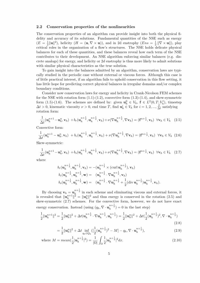
2.2 Conservation properties of the nonlinearities

The conservation properties of an algorithm can provide insight into both the physical fi-delity and accuracy of its solutions. Fundamental quantities of the NSE such as energy(E = 1

2‖u‖2), helicity (H = (u,∇ × u)), and in 2d enstrophy (Ens = 12 ‖∇ × u‖), play

critical roles in the organization of a flow’s structures. The NSE holds delicate physicalbalances for each of these quantities, and these balances reveal how each term of the NSEcontributes to their development. An NSE algorithm enforcing similar balances (e.g. dis-crete analogs) for energy, and helicity or 2d enstrophy is thus more likely to admit solutionswith similar physical characteristics as the true solution.

To gain insight into the balances admitted by an algorithm, conservation laws are typi-cally studied in the periodic case without external or viscous forces. Although this case isof little practical interest, if an algorithm fails to uphold conservation in this flow setting, ithas little hope for predicting correct physical balances in irregular domains and/or complexboundary conditions.

Consider now conservation laws for energy and helicity in Crank-Nicolson FEM schemesfor the NSE with rotation form (1.1)-(1.2), convective form (1.3)-(1.4), and skew-symmetricform (1.5)-(1.6). The schemes are defined by: given u0

h ∈ Vh, f ∈ L2(0, T ;V ′h), timestep

∆t > 0, kinematic viscosity ν > 0, end time T , find uih ∈ Vh for i = 1, 2, ..., T

∆t satisfyingrotation form:

1∆t

(un+1h −un

h,vh) +br(un+ 1

2h ,u

n+ 12

h ,vh)+ν(∇un+ 1

2h ,∇vh) = (fn+ 1

2 ,vh) ∀vh ∈ Vh (2.5)

Convective form:1

∆t(un+1

h − unh,vh) + bc(u

n+ 12

h ,un+ 1

2h ,vh) + ν(∇u

n+ 12

h ,∇vh) = (fn+ 12 ,vh) ∀vh ∈ Vh (2.6)

Skew-symmetric:

1∆t

(un+1h −un

h,vh) +bs(un+ 1

2h ,u

n+ 12

h ,vh)+ν(∇un+ 1

2h ,∇vh) = (fn+ 1

2 ,vh) ∀vh ∈ Vh (2.7)

where

br(un+ 1

2h ,u

n+ 12

h ,vh) = −(un+ 1

2h × (curlu

n+ 12

h ),vh)

bc(un+ 1

2h ,u

n+ 12

h ,w) = (un+ 1

2h · ∇u

n+ 12

h ,vh)

bs(un+ 1

2h ,u

n+ 12

h ,w) = (un+ 1

2h · ∇u

n+ 12

h +12(div u

n+ 12

h )un+ 1

2h ,vh).

By choosing vh = un+ 1

2h in each scheme and eliminating viscous and external forces, it

is revealed that ‖un+1h ‖2 = ‖un

h‖2 and thus energy is conserved in the rotation (2.5) andskew-symmetric (2.7) schemes. For the convective form, however, we do not have exact

energy conservation. Instead (using (qh,∇ · un+ 12

h ) = 0 in the last step)

12‖un+1

h ‖2 =12‖un

h‖2 + ∆t(un+ 1

2h · ∇u

n+ 12

h ,un+ 1

2h ) =

12‖un

h‖2 + ∆t(12(u

n+ 12

h )2,∇ · un+ 12

h )

(2.8)

=12‖un

h‖2 + ∆t infqh∈Qh

([12(u

n+ 12

h )2 −M ]− qh,∇ · un+ 12

h ), (2.9)

where M = mean(12|un+ 1

2h |2) =

1|Ω|

∫

Ω

12|un+ 1

2h |2dx. (2.10)

5

Exact energy conservation in the convective form scheme (2.6) thus depends on divun+ 1

2h

(and the resolution of the key component of the Bernoulli pressure in the pressure space),which is nonzero since incompressibility is only weakly enforced. Hence it is possible (andwell known to be likely) that these “small” errors in the energy balance at each time stepcan accumulate and significantly alter the solution.

Regarding helicity (3d) and enstrophy (2d) conservation, by choosing vh = PVh(curluh)

in the three schemes, it can be seen that none of the schemes conserve helicity; indeed all ofthe three nonlinearities alters helicity. However, it was shown in [27] that if the curl in therotation form nonlinearity is replaced with the Vh-projected curl, then the rotation schemewill conserve helicity. To our knowledge, no such alterations can be made to (2.6) or (2.7)to maintain physical treatment of helicity. It is pointed out in [14] that for finite differenceschemes, the rotation form shows superior conservation properties to the convective formin that rotation form conserves mean momentum, energy, helicity, enstrophy and vorticityversus just mean momentum and energy for the convective form.

2.3 Grad− div stabilization

The three forms of the nonlinearity, and thus the three schemes (2.5),(2.6), and (2.7) areequivalent when divuh = 0. Since this condition is only weakly enforced, divuh maygrow large enough to cause significant differences between the schemes; as our numericalexperiments show, this is especially true near boundaries for the rotation form. Grad− divstabilization can help to correct this error for steady, incompressible flow [24], and throughour experiments in Sections 3.2 and 3.4 we show that this stabilization technique is alsoeffective for unsteady flow.

To understand better the role of adding the grad − div term to the finite elementformulation we consider the model case of the Stokes problem:

−ν∆u +∇p = f , and div u = 0 in Ω,

u = 0 on ∂Ω.(2.11)

Given normal velocity-pressure finite element spaces Uh, Qh, satisfying the discrete inf-supcondition, the grad− div stabilized FEM for this problem is: Pick stabilization parameterγ ≥ 0 and find uh, ph ∈ Uh, Qh satisfying

ν(∇uh,∇vh) + γ(div uh, div vh)− (ph, div vh) + (qh,div uh)= (f ,vh), ∀ vh, qh ∈ Uh, Qh. (2.12)

For the case γ = 0 a common argument is to rescale the equations by p = ν−1p, f = ν−1f .This leads to a parameter-independent Stokes problem with a new pressure variable andright-hand side. One can then use known results for this Stokes problem (in u, p) andtransform back to the u, p variables. The first and most basic result in the numericalanalysis of the (parameter-independent) rescaled Stokes problem is that

‖∇(u− uh)‖ ≤ C( infvh∈Uh

‖∇(u− vh)‖+ infqh∈Qh

‖p− qh‖).

Converting back to the original dependent variables gives

‖∇(u− uh)‖ ≤ C( infvh∈Uh

‖∇(u− vh)‖+1ν

infqh∈Qh

‖p− qh‖). (2.13)

6

This has the interpretation that: Velocity Error ∼Re * Pressure Error. For example, afurther development of these estimates give the error bound in the rescaled variables

‖∇(u− uh)‖+ ‖p− ph‖ ≤ Ch(‖∇∇u‖+ ‖∇p‖).

In the original variables this immediately yields

‖∇(u− uh)‖+1ν‖p− ph‖ ≤ Ch(‖∇∇u‖+

1ν‖∇p‖), (2.14)

with a constant C that is independent of ν. Numerical experiments, see [23], shows that(2.14) is sharp. If γ > 0, (2.12) cannot be so rescaled unless γ = ν. Otherwise, for (2.12)the following estimate is valid ([23], Th. 4.2 and 4.3)

ν12 ‖∇(u− uh)‖+ γ

12 ‖div (u− uh)‖+ ‖p− ph‖ ≤ Ch((ν

12 + γ

12 )‖∇∇u‖+ ‖∇p‖) (2.15)

with a constant C that is independent of ν and γ. Estimates (2.14) and (2.15) suggest thatfor small enough ν we have

for γ = 0 : ‖∇(u− uh)‖ ' h (‖∇∇u‖+1ν‖∇p‖)

for γ = 1 : ‖∇(u− uh)‖ ' h√ν

(‖∇∇u‖+ ‖∇p‖).

Thus, large pressure gradients compared to the velocity second derivatives may lead to apoor convergence of the finite element velocity if one does not include grad − div stabi-lization. Otherwise, the dependence of ‖∇(u− uh)‖ on ν is much milder.

3 Three numerical experiments

We consider three carefully chosen examples that, we believe, give strong support for thescenario of accuracy loss described in the introduction. We use the software FreeFem++ [13]to run the numerical tests. The models are discretized with the Crank-Nicolson method intime and with the Taylor-Hood finite elements (continuous piecewise quadratic polynomialsfor the velocity and linears for the pressure) in space; the nonlinear system is solved by afixed point iteration.

3.1 Test 1: Poiseuille flow

In Ω = (0, 4) × (0, 1), a parabolic inflow v(x, t) = 0 and u(x, y, t) = 12ν y(1 − y) (at x = 0)

is prescribed. No-slip boundary conditions are given at the top and bottom, and the do-nothing boundary condition is prescribed at the outflow. The exact solution is well knownto be v(x, y) = 0, u(x, y) = 1

2ν y(1 − y), p(x, y) = −x + 4, and we take it as our initialcondition. The key conserved quantity in the flow is the flux through any cross sectiongiven by

Q(x) =∫

0<y<1u(x, y)dy =

112ν

Note that u = (u, v) and p are in the finite element spaces so that we expect thatdiscretization of the convective and skew symmetric form of the NSE will have very smallerrors (comparable to the errors from numerical integration and solution of the linear and

7

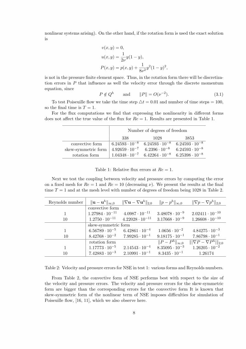
nonlinear systems arising). On the other hand, if the rotation form is used the exact solutionis

v(x, y) = 0,

u(x, y) =12ν

y(1− y),

P (x, y) = p(x, y) +1

8ν2y2(1− y)2,

is not in the pressure finite element space. Thus, in the rotation form there will be discretiza-tion errors in P that influence as well the velocity error through the discrete momentumequation, since

P /∈ Qh and ‖P‖ = O(ν−2). (3.1)

To test Poiseuille flow we take the time step 4t = 0.01 and number of time steps = 100,so the final time is T = 1.

For the flux computations we find that expressing the nonlinearity in different formsdoes not affect the true value of the flux for Re = 1. Results are presented in Table 1.

Number of degrees of freedom

338 1028 3853convective form 6.24593 · 10−8 6.24593 · 10−8 6.24593 · 10−8

skew-symmetric form 4.92659 · 10−7 6.2396 · 10−8 6.24593 · 10−8

rotation form 1.04348 · 10−7 6.42264 · 10−8 6.25398 · 10−8

Table 1: Relative flux errors at Re = 1.

Next we test the coupling between velocity and pressure errors by computing the erroron a fixed mesh for Re = 1 and Re = 10 (decreasing ν). We present the results at the finaltime T = 1 and at the mesh level with number of degrees of freedom being 1028 in Table 2.

Reynolds number ‖u− uh‖∞,0 ‖∇u−∇uh‖2,0 ‖p− ph‖∞,0 ‖∇p−∇ph‖2,0

convective form1 1.27984 · 10−11 4.0987 · 10−11 3.48078 · 10−9 2.02411 · 10−10

10 1.2750 · 10−11 4.22028 · 10−11 3.17668 · 10−9 1.26608 · 10−10

skew-symmetric form1 6.56789 · 10−5 6.42861 · 10−4 1.0656 · 10−2 4.84275 · 10−3

10 8.42768 · 10−2 7.99285 · 10−1 9.18175 · 10−1 7.86798 · 10−1

rotation form ‖P − P h‖∞,0 ‖|∇P −∇P h|‖2,0

1 1.17773 · 10−5 2.14543 · 10−4 8.35095 · 10−3 1.26205 · 10−2

10 7.42883 · 10−3 2.10991 · 10−1 8.3435 · 10−1 1.26174

Table 2: Velocity and pressure errors for NSE in test 1: various forms and Reynolds numbers.

From Table 2, the convective form of NSE performs best with respect to the size ofthe velocity and pressure errors. The velocity and pressure errors for the skew-symmetricform are bigger than the corresponding errors for the convective form It is known thatskew-symmetric form of the nonlinear term of NSE imposes difficulties for simulation ofPoiseuille flow, [16, 11], which we also observe here.

8

We also observe that while the velocity errors are smaller for the rotation form comparedto the skew-symmetric form, the error in the (Bernoulli) pressure gradient is larger than the(usual) pressure gradient error of the skew-symmetric form. Note that for rotation form,the pressure error ‖p− ph‖∞,0 and the velocity error ‖∇(u− uh)‖2,0 seem to scale like Re3,and ‖u− uh‖∞,0 seems to scale like Re2. Poor scaling with Re can be improved in the caseof Stokes and rotation form steady NSE with the use of grad− div stabilization, and is ourmotivation in later test problems to use this stabilization.

3.2 Test 2: Resolution vs. nonlinearity

The relative importance of resolution of pressures vs. nonlinearity can be tested by arti-ficially reversing p and P in Test 1 in a (completely) synthetic test problem. Thus, wetake:

u(x, y) =12ν

y(1− y), v(x, y) = 0 P (x, y) = −x + 4

so thatp(x, y) = −x + 4− 1

8ν2y2(1− y)2,

These are inserted in the Navier-Stokes equations to obtain a right-hand side f = f(x, y, ν):

f(x, y; ν) := (0,1

4ν2(y2(1− y)− y(1− y)2) )T

The resolution of p vs. P is exactly reversed from Test 1. We present the error behavior atthe final time T = 1 and at the mesh level with number of degrees of freedom being 1028in Table 3.

Reynolds number ‖u− uh‖∞,0 ‖∇u−∇uh‖2,0 ‖p− ph‖∞,0 ‖∇p−∇ph‖2,0

convective form1 6.51439 · 10−5 6.66111 · 10−4 1.06432 · 10−2 1.34122 · 10−2

10 4.50658 · 10−2 4.76032 · 10−1 8.92802 · 10−1 1.3361skew-symmetric form

1 1.19698 · 10−5 2.18059 · 10−4 3.71786 · 10−4 1.2624 · 10−2

10 7.65648 · 10−3 2.15944 · 10−1 3.90984 · 10−2 1.26198rotation form ‖P − P h‖∞,0 ‖∇P −∇P h‖2,0

1 3.19832 · 10−12 1.05429 · 10−11 9.36552 · 10−6 5.77438 · 10−11

10 3.19792 · 10−12 1.08799 · 10−11 9.35505 · 10−5 3.40516 · 10−11

Table 3: Velocity and pressure errors for NSE in test 2: various forms and Reynolds nume-bers.

Table 3 shows that discretization errors are present if the solution does not belong tothe finite element space. The computed errors from Test 2 are the mirror image (up tothe preset accuracy used for the various linear and nonlinear iterative solvers’ stoppingcriteria )of the error behavior in the previous test. Thus it is clear that, without grad− divstabilization, in the rotation form it is the resolution of the Bernoulli pressure determinethe quality of the overall velocity approximation.

9

3.3 Test 3: Flow around a cylinder

Next we consider the benchmark problem of flow around a circular cylinder offset slightlyin a channel, from [28], see Figure 1. The primary feature is the von Karman vortex street.To explore resolution vs. solution quality for the two formulations we test at a Reynoldsnumber slightly above the critical one for vortex shedding and we have the simple test:Vortex street formed yes or no.

The time dependent inflow and outflow profile are

u1(0, y, t) = u1(2.2, y, t) =6

0.412sin(π t/8)y(0.41− y)

u2(0, y, t) = u2(2.2, y, t) = 0.

No slip boundary conditions are prescribed along the top and bottom walls and the initialcondition is u(x, y, 0) = 0. The viscosity is set at ν = 10−3, the external force f = 0, andthe Reynolds number of the flow, based on the diameter of the cylinder and on the meanvelocity inflow is 0 ≤ Re ≤ 100. The time step is chosen to be ∆t = 0.005.

Figure 1: Cylinder Domain

Freefem generated two Delaunay meshes for testing this problem, the finest of which isable to resolve the problem for the NSE in either (rotation or skew symmetric) form. Theseare shown in Figure 2.

Figure 2: Shown above are two levels of mesh refinement provided by Freefem for computingflow around a cylinder. The meshes provide, respectively, 14,455, and 56,702 degrees offreedom for the computations.

The velocity field calculated on mesh 1 is shown in Figures 3 and 4. Note that

10

• with the skew symmetric form the vortex street is well defined already on mesh 1(coarse mesh);

• with the rotation form the mesh 1 simulations fails.

• with the rotation form and grad − div stabilization, the mesh 1 simulation forms avortex street

0 0.5 1 1.5 20

0.1

0.2

0.3

0.4

0 0.5 1 1.5 20

0.1

0.2

0.3

0.4

0 0.5 1 1.5 20

0.1

0.2

0.3

0.4

0 0.5 1 1.5 20

0.1

0.2

0.3

0.4

0 0.5 1 1.5 20

0.1

0.2

0.3

0.4

0 0.5 1 1.5 20

0.1

0.2

0.3

0.4

Figure 3: Shown above is the velocity field at times t = 2, 3, 5, 6, 7, 8 for the NSE solvedon mesh 1 with the skew-symmetric form of the nonlinearity. The vortex street formssuccessfully.

The pressure (and accuracy thereof) is critical for the formation of the vortex street. Totest the resolution hypothesis, we move to mesh 2, which fully resolves both formulations.Figures 5 and 6 plot p (from skew-symmetric formulation) and P (from rotation formula-tion), respectively, and from these plots we see indication that P contains much smaller

11

0 0.5 1 1.5 20

0.1

0.2

0.3

0.4

0 0.5 1 1.5 20

0.1

0.2

0.3

0.4

0 0.5 1 1.5 20

0.1

0.2

0.3

0.4

0 0.5 1 1.5 20

0.1

0.2

0.3

0.4

0 0.5 1 1.5 20

0.1

0.2

0.3

0.4

0 0.5 1 1.5 20

0.1

0.2

0.3

0.4

Figure 4: Shown above is the velocity field at times t = 2, 3, 5, 6, 7, 8 for the NSE solved onmesh 1 with the rotation form of the nonlinearity. The vortex street fails to form.

transition regions than p. The difference can also be seen when the L2 norm of ∇p, ∇P areplotted versus time, in Figure 7.

Figure 8 shows the effect of the grad − div stabilization of the solution computed inmesh 1 with γ = 1 and the rotation form. Without the stabilization, the rotation form isunable to predict the correct behavior. With grad− div stabilization, the correct behavioris predicted already on mesh 1.

12

0 0.5 1 1.5 20

0.1

0.2

0.3

0.4

0 0.5 1 1.5 20

0.1

0.2

0.3

0.4

0 0.5 1 1.5 20

0.1

0.2

0.3

0.4

0 0.5 1 1.5 20

0.1

0.2

0.3

0.4

0 0.5 1 1.5 20

0.1

0.2

0.3

0.4

0 0.5 1 1.5 20

0.1

0.2

0.3

0.4

Figure 5: Shown above is the Bernoulli pressure P at times t = 2, 4, 5, 6, 7, 8 from NSErotation Form on mesh 2, where a vortex street forms successfully.

3.4 Test 4: Channel flow over a forward and backward facing step

The most distinctive feature of this common test problem is the formation and detachmentof vortices behind the step (a more detailed discussion of this test problem can be found inGunzburger [10] and John and Liakos [17]). We study the behavior of NSE schemes usingthe convective form, the skew-symmetric form, the rotation form, and the rotation formwith grad-div stabilization (with γ = 0.5). The simulations are performed on the samedomain , which is meshed with Delaunay triangulation (provided by Freefem), yielding24,598 degree of freedom systems. We set Re = 600 (slightly above the critical Reynoldsnumber for which eddies are known to shed), and take timestep ∆t = 0.005.

Results are presented for a parabolic inflow profile, given by u = (u1, u2)T , with u1 =y(10− y)/25, u2 = 0. The no-slip boundary condition is prescribed on the top and bottom

13

0 0.5 1 1.5 20

0.1

0.2

0.3

0.4

0 0.5 1 1.5 20

0.1

0.2

0.3

0.4

0 0.5 1 1.5 20

0.1

0.2

0.3

0.4

0 0.5 1 1.5 20

0.1

0.2

0.3

0.4

0 0.5 1 1.5 20

0.1

0.2

0.3

0.4

0 0.5 1 1.5 20

0.1

0.2

0.3

0.4

Figure 6: Shown above is the usual pressure p at times t = 2, 4, 5, 6, 7, 8 from NSE Skew-Symmetric Form on mesh 2, where a vortex street forms successfully.

boundary, as well as on the step. At the outflow the standard do-nothing boundary conditionis imposed.

We conclude that the NSE with the convective and skew-symmetric forms of the nonlin-earity give the appropriate shedding of eddies behind the step. The NSE with the rotationform fails to describe the flow correctly, but the rotation form with grad− div stabilizationsuccessfully captures the generation and detachment of eddies.

As an interesting but tangential observation, the do-nothing outflow boundary conditionis not satisfactory for use with the rotation form which means that, until the outflowboundary issue is resolved for the rotation form, for practical purposes one has to use adomain which is sufficiently large so that the do-nothing boundary condition is applied farenough from region of interest. As we see in Figure 12, numerical artifacts are seen near

14

0 1 2 3 4 5 6 7 80

2

4

6

8

10

12

14

16

t

grad p, mesh 2grad p, mesh 1grad P, mesh 2grad P, mesh 1

Figure 7: Shown here is a comparison of the L2 norm of pressure gradients from simulationsof 2d flow around a cylinder on Meshes 1 and 2. P denoted Bernoulli pressure from therotation form scheme, and usual pressure from the convective form scheme is denoted by p.It is clear that ∇P is larger during the development (or lack thereof) of a vortex street.

the outflow boundary.

4 Conclusions

Although the convective, skew-symmetric and rotation forms of the nonlinearity are equiv-alent in the continuous NSE, in finite element discretizations the rotation form offers betterphysical properties (in terms of conservation laws), superior properties for iterative algo-rithm development, is typically more stable than the convective form, and is less expensivethan computing the skew-symmetric form.

However, using rotation form requires the use of the Bernoulli pressure, which is gener-ically significantly more complex than the usual pressure of the convective and skew-symmetric forms. Bernoulli pressure is thus not as easily resolved, which causes significantlyworse results in our benchmark problems for the rotation form scheme. Fortunately, withthe use of grad− div stabilization, the inaccuracy in the Bernoulli pressure associated withusing rotation form seems to be localized in the pressure error and have much reduced (oreven minimal) effect upon the velocity error.

15

0 0.5 1 1.5 20

0.1

0.2

0.3

0.4

0 0.5 1 1.5 20

0.1

0.2

0.3

0.4

0 0.5 1 1.5 20

0.1

0.2

0.3

0.4

0 0.5 1 1.5 20

0.1

0.2

0.3

0.4

0 0.5 1 1.5 20

0.1

0.2

0.3

0.4

0 0.5 1 1.5 20

0.1

0.2

0.3

0.4

Figure 8: Shown above is the velocity field at times t = 2, 3, 5, 6, 7, 8 for the NSE solved onmesh 1 with the rotation form of the nonlinearity and with grad − div stabilization. Herethe vortex street forms succesfully.

16

T=10

0 10 20 30 400

2

4

6

8

10 T=20

0 10 20 30 400

2

4

6

8

10

T=30

0 10 20 30 400

2

4

6

8

10T=40

0 10 20 30 400

2

4

6

8

10

Figure 9: NSE with convective form of nonlinearity

T=10

0 10 20 30 400

2

4

6

8

10 T=20

0 10 20 30 400

2

4

6

8

10

T=30

0 10 20 30 400

2

4

6

8

10T=40

0 10 20 30 400

2

4

6

8

10

Figure 10: NSE with skew-symmetric form of nonlinearity

T=10

0 10 20 30 400

2

4

6

8

10 T=20

0 10 20 30 400

2

4

6

8

10

T=30

0 10 20 30 400

2

4

6

8

10T=40

0 10 20 30 400

2

4

6

8

10

Figure 11: NSE with rotation form of nonlinearity

17

T=10

0 10 20 30 400

2

4

6

8

10 T=20

0 10 20 30 400

2

4

6

8

10

T=30

0 10 20 30 400

2

4

6

8

10T=40

0 10 20 30 400

2

4

6

8

10

Figure 12: NSE with grad− div stabilization for the rotation form

18

References

[1] M. Benzi and J. Liu, An Efficient Solver for the Incompressible Navier-Stokes Equa-tions in Rotation Form, SIAM J. Scientific Computing, 29 (2007), pp. 1959-1981.

[2] E. Burman and A. Linke, Stabilized finite element schemes for incom-pressible flow using Scott–Vogelius elements, Appl. Numer. Math. (2007),doi:10.1016/j.apnum.2007.11.001

[3] M. Braack, E. Burman, V. John, and G. Lube, Stabilized finite element methods forthe generalized Oseen problem, Comput. Methods Appl. Mech. Eng., 196 (2007), pp.853–866.

[4] Q. Chen S. Chen and G. Eyink, The joint cascade of energy and helicity in threedimensional turbulence. Physics of Fluids, 15(2):361–374, 2003.

[5] C. Canuto, M.Y. Hussaini, A. Quarteroni, and T. A. Zang, Spectral methods in fluiddynamics, Springer, Berlin 1988.

[6] P. Ditlevson and P. Guiliani, Cascades in helical turbulence. Physical Review E, 63,2001.

[7] H. C. Elman, D. J. Silvester, and A. J. Wathen, Finite Elements and Fast IterativeSolvers: with Applications in Incompressible Fluid Dynamics, Numerical Mathematicsand Scientific Computation, Oxford University Press, Oxford, UK, 2005.

[8] L. P. Franca and S. L. Frey, Stabilized finite element methods: II. The incompressibleNavier–Stokes equations, Comput. Methods Appl. Mech. Engrg., 99 (1992), pp. 209–233.

[9] P. Gresho and R. Sani, Incompressible Flow and the Finite Element Method, Vol 2.,Wiley, 2000.

[10] M.D. Gunzburger, Finite Element Methods for Viscous Incompressible Flows - A Guideto Theory, Practices, and Algorithms, Academic Press, 1989.

[11] J.G. Heywood, R. Rannacher and S. Turek, Artificial boundaries and flux and pressureconditions for the incompressible Navier-Stokes equations, Int. J. Numer. MathodsFluids, 22(1996), pp.325-352

[12] P. Hansbo and A. Szepessy, A velocity-pressure streamline diffusion method for the in-compressible Navier-Stokes equations, Comput. Methods Appl. Mech. Engrg., 84 (1990),pp. 175–192.

[13] F. Hecht and O. Pironneau, FreeFem++ webpage: http://www.freefem.org.

[14] K. Horiuti, Comparison of conservative and rotation forms in large eddy simulation ofturbulent channel flow, J. Comp. Phys. 71(1987) 343-370.

[15] K.Horiuti and T. Itami, Truncation error analysis of the rotation form of convectiveterms in the Navier-Stokes equations, Journal of Computational Physics, 145 (1998),pp. 671–692.

19

[16] V. John, Large Eddy Simulation of Turbulent Incompressible Flows. Analytical andNumerical Results for a Class of LES Models, Lecture Notes in Computational Scienceand Engineering, vol. 34, Springer-Verlag Berlin, Heidelberg, New York, 2004.

[17] V. John and A. Liakos, Time dependent flow across a step: the slip with frictionboundary condition, Int. J. Numer. Meth. Fluids, 50, (2006), 713-731.

[18] W. Layton, C. Manica, M. Neda and L. Rebholz, Numerical Analysis and Computa-tional comparisons of the NS-alpha and NS-omega regularizations, Technical report,TR-MATH 08-01, Math Dept. , Univ of Pittsburgh, 2008.

[19] G. Lube and M. Olshanskii, Stable finite element calculations of incompressible flowsusing the rotation form of convection, IMA J. Num. Anal., 22 (2002) 437-461.

[20] G. Matthies and G. Lube, On streamline-diffusion methods of inf-sup stable discretiza-tions of the generalized Oseen problem, Preprint 2007-02, Institute Numerische undAngewandte Mathematik, Georg-August-Universi¨at G¨ottingen, 2007.

[21] G. Matthies and L. Tobiska, Local projection type stabilization applied to inf-supstable discretizations of the Oseen problem, Preprint 47/2007, Dept. Math., Otto-von-Guericke-Universitat Magdeburg, 2007.

[22] R. D. Moser and P. Moin, The effects of curvature in wall bounded flows, J. FluidMech., 175 (1987), 479-510.

[23] M.A. Olshanskii, A. Reusken, Grad-Div stabilization for the Stokes equations, Math-ematics of Computation, 73 (2004), P. 1699–1718.

[24] M.A. Olshanskii, A low order Galerkin finite element method for the Navier-Stokesequations of steady incompressible flow: A stabilization issue and iterative methods,Comp. Meth. Appl. Mech. Eng., 191 (2002), P. 5515–5536

[25] M.A. Olshanskii, A. Reusken, Navier-Stokes equations in rotation form: a robustmultigrid solver for the velocity problem, SIAM J. Scientific Computing, 23 (2002),P. 1682–1706

[26] M.A. Olshanskii, Iterative solver for Oseen problem and numerical solution of incom-pressible Navier-Stokes equations, Num. Linear Algebra Appl., 6 (1999), P. 353–378.

[27] L. Rebholz, An energy and helicity conserving finite element scheme for the Navier-Stokes equations. SIAM Journal on Numerical Analysis, 45(4):1622–1638, 2007.

[28] M. Shafer and S. Turek, Benchmark computations of laminar flow around cylinder, InFlow Simulation with High-Performance Computers II, Vieweg, 1996.

[29] L. Tobiska and G. Lube, A modified streamline diffusion method for solving the sta-tionary Navier-Stokes equations, Numer. Math., 59 (1991), pp. 13–29.

[30] T.A. Zang, On the rotation and skew-symmetric forms for incompressible flow simula-tions, Appl. Num. Math. 7 (1991) 27-40.

20