On Surrogate Dimension Reduction for Measurement Error ...

On Surrogate Dimension Reduction for Measurement Error Regression: An Invariance LawAuthor(s): Bing Li and Xiangrong YinSource: The Annals of Statistics, Vol. 35, No. 5 (Oct., 2007), pp. 2143-2172Published by: Institute of Mathematical StatisticsStable URL: http://www.jstor.org/stable/25464576 .Accessed: 13/09/2011 09:40

Your use of the JSTOR archive indicates your acceptance of the Terms & Conditions of Use, available at .http://www.jstor.org/page/info/about/policies/terms.jsp

JSTOR is a not-for-profit service that helps scholars, researchers, and students discover, use, and build upon a wide range ofcontent in a trusted digital archive. We use information technology and tools to increase productivity and facilitate new formsof scholarship. For more information about JSTOR, please contact [email protected].

Institute of Mathematical Statistics is collaborating with JSTOR to digitize, preserve and extend access to TheAnnals of Statistics.

http://www.jstor.org

http://www.jstor.org/action/showPublisher?publisherCode=ims

http://www.jstor.org/stable/25464576?origin=JSTOR-pdf

http://www.jstor.org/page/info/about/policies/terms.jsp

The Annals of Statistics 2007, Vol. 35, No. 5, 2143-2172 DOI: 10.1214/009053607000000172 ? Institute of Mathematical Statistics, 2007

ON SURROGATE DIMENSION REDUCTION FOR MEASUREMENT ERROR REGRESSION: AN INVARIANCE LAW

By Bing Li1 and Xiangrong Yin

Pennsylvania State University and University of Georgia

We consider a general nonlinear regression problem where the predictors contain measurement error. It has been recently discovered that several well

known dimension reduction methods, such as OLS, SIR and pHd, can be per formed on the surrogate regression problem to produce consistent estimates

for the original regression problem involving the unobserved true predictor. In this paper we establish a general invariance law between the surrogate and

the original dimension reduction spaces, which implies that, at least at the

population level, the two dimension reduction problems are in fact equiva lent. Consequently we can apply all existing dimension reduction methods

to measurement error regression problems. The equivalence holds exactly for

multivariate normal predictors, and approximately for arbitrary predictors. We also characterize the rate of convergence for the surrogate dimension re

duction estimators. Finally, we apply several dimension reduction methods

to real and simulated data sets involving measurement error to compare their

performances.

1. Introduction. We consider dimension reduction for regressions in which

the predictor contains measurement error. Let X be a p -dimension random vec

tor representing the true predictor and Y be a random variable representing the

response. In many applications we cannot measure X (e.g., blood pressure) accu

rately, but instead observe a surrogate r-dimensional predictor W that is related to X through the linear equation

(1) W = y + rTX + 8,

where y is an r-dimensional nonrandom vector, r is a p by r nonrandom matrix and S is an r-dimensional random vector independent of (X, Y). The goal of the

regression analysis is to find the relation between the response Y and the true, but unobserved, predictor X. This type of regression problem frequently occurs in

practice and has been the subject of extensive studies, including, for example, those that deal with linear models (Fuller [15]), generalized linear models (Carroll [2], Carroll and Stefanski [5]), nonlinear models (Carroll, Ruppert and Stefanski [4]) and nonparametric models (see Pepe and Fleming [23]).

Received June 2005; revised November 2006.

Supported in part by NSF Grants DMS-02-04662 and DMS-04-05681. AMS 2000 subject classifications. 62G08, 62H12.

Key words and phrases. Central spaces, central mean space, invariance, regression graphics, sur

rogate predictors and response, weak convergence in probability.

2143

2144 B.LI AND X.YIN

Typically there is an auxiliary sample which provides information about the re

lation between the original predictor X and the surrogate predictor W, for example, by allowing us to estimate T>wx = cov(W, X). Using this covariance estimate we can adjust the surrogate predictor W to align it as much as possible with the true

predictor X. At the population level this is realized by regressing W on X, that is,

adjusting W to U = ^xw^w w> where ^xw = cov(X, W) and Sw = var(W).

The fundamental question that will be answered in this paper is this: If we per form a dimension reduction operation on the surrogate regression problem of Y versus U, will the result correctly reflect the relation between Y and the true pre dictor XI

In the classical setting where the true predictor X is observed, the dimension reduction problem can be briefly outlined as follows. Suppose that Y depends on

X only through a lower dimensional vector of linear combinations of X, say fiTX, where fi is a p by d matrix with d < p. Or more precisely, suppose that Y is

independent of X conditioning on fiTX, which will be denoted by

(2) YALX\fiTX.

The goal of dimension reduction is to estimate the directions of column vectors

of fi, or the column space of fi. Note that the above relation will not be affected if

fi is replaced by fi A for any nonsingular p x p matrix A. This is why the column

space of fi, rather than fi itself, is the object of interest in dimension reduction.

A dimension reduction space provides us with a set of important predictors among all the linear combinations of X, with which we could perform exploratory data

analysis or finer regression analysis without having to fit a nonparametric regres sion over a large number of predictors. Classical estimators of the dimension re

duction space include ordinary least square (OLS) (Li and Duan [21], Duan and Li

[13]), sliced inverse regression (SIR) (Li [19]), principle Hessian directions (pHd) (Li [20]) and the sliced inverse variance estimators (SAVE) (Cook and Weisberg [11]).

It has been discovered that some of these dimension reduction methods can be

performed on the adjusted surrogate predictor U to produce consistent estimates

of at least some vectors in the column space of fi in (2) that describes the relation

between Y and the (unobserved) true predictor X. The first paper in this area is

Carroll and Li [3], which demonstrated this phenomenon for OLS and SIR, and

introduced the corresponding estimators of fi in the measurement error context.

More recently, Lue [22] established that the pHd method, when applied to the sur

rogate problem (U, Y), also yields consistent estimators of vectors in the column

space of fi. This work opens up the possibility of using available dimension reduc

tion techniques to estimate fi by simply pretending U is the true predictor X.

In this paper we will establish a general equivalence between the dimension

reduction problem of Y versus U and that of Y versus X. That is,

(3) YALX\fiTX if and only if Y _IL U\fiTU.

SURROGATE DIMENSION REDUCTION 2145

This means that dimension reduction for the surrogate regression problem of Y versus U and that for the original regression problem of Y versus X are in fact

equivalent at the population level. Thus the phenomena discovered by the above

work are special cases of a very general invariance pattern?we can, in fact, ap

ply any consistent dimension reduction method to the surrogate regression prob lem of Y versus U to produce consistent dimension reduction estimates for the

original regression problem of Y versus X. This fundamental relation is of prac tical importance, because OLS, SIR and pHd have some well-known limitations.

For example, SIR does not perform well when the regression surface is symmet ric about the origin, and pHd does not perform well when the regression surface

lacks a clear quadratic pattern (or what is similar to it). New methods have recently been developed that can, in different respects and to varying degrees, remedy these

shortcomings; see, for example, Cook and Li [9, 10], Xia et al. [25], Fung et al.

[16], Yin and Cook [27, 28] and Li, Zha and Chiaromonte [18]. This equivalence allows us to choose among the broader class of dimension reduction methods to

tackle the difficult situations in which the classical methods become inaccurate. Sometimes the main purpose of the regression analysis is to infer the condi

tional mean E(Y\X) or more generally conditional moments such as E(Yk\X). For example, in generalized linear models we are mainly interested in estimating the conditional mean E(Y\X), and for regression with heteroscedasticity we may be interested in both the conditional mean E(Y\X) and the conditional variance

var(F|Z). In these cases it is sensible to treat the conditional moments such as

E(Y\X) and var(y|Z) as the objects of interest and the rest of the conditional distribution f(Y\X) as the (infinite dimensional) nuisance parameter, and refor mulate the dimension reduction problem to reflect this hierarchy. This was carried out in Cook and Li [9] and Yin and Cook [26], which introduced the notions of the central mean space and central moment space as well as methods to estimate them. If there is a p by d matrix fi with d < p such that E(Y\X) = E(Y\fiTX), then we call the column space of ft a dimension reduction space for the conditional mean

E(Y\X). More generally, the dimension reduction space for the fcth conditional moment E(Yk\X) is defined as above with Y replaced by Yk. In this paper we

will also establish the equivalence between the dimension reduction spaces for the ^-conditional moments of the surrogate and the original regressions. That is,

(4) E(Yk\X) = E(Yk\/3TX) if and only if E(Yk\U) = E(Yk\pTU). The above invariance relations will be shown to hold exactly under the assump

tion that X and 8 are multivariate normal; a similar assumption was also used in Carroll and Li [3] and Lue [22]. For arbitrary predictor and measurement error, we will establish an approximate invariant relation. This is based on the fact that, when p is modestly large, most projections of a random vector are approximately normal (Diaconis and Freedman [12], Hall and Li [17]). Simulation studies indi cate that the approximate invariance law holds for surprisingly small p (as small as 6) and for severely nonnormal predictors.

2146 B.LI AND X.YIN

This paper will be focused on the dimension reduction problems defined

through relationships such as Y JL X\fiTX. A more general problem can be for mulated as Y JL X\t(X), where t(X) is a (possibly nonlinear) function of X; see Cook [8]. Surrogate dimension reduction in this general sense is not covered by this paper, and remains an important open problem.

In Section 2 we introduce some basic issues and concepts related to measure ment error problems and dimension reduction, as well as some machinery that will be repeatedly used in our further exposition. Equivalence (3) will be established in Section 3 for the case where r in (1) is a p by p nonsingular matrix. Equiva lence (3) for general T will be shown in Section 4. In Section 5 we will establish

equivalence (4). The approximate equivalence for general predictors and measure ment errors will be developed in Section 6. In Section 7 we will turn our attention to a general estimation procedure for surrogate dimension reduction and study its

convergence rate. In Section 8 we conduct a simulation study to compare different

surrogate dimension reduction methods. In Section 9 we apply the invariance law to analyze a managerial behavior data set (Fuller [15]) that involves measurement errors. Some technical results will be proved in the Appendix.

2. Preliminaries. In this section we lay out some basic concepts and notation. For a pair of random vectors V\ and V2, we will use Ev^ y2 to denote the covariance matrix cov(Vi, V2), and for a random vector V, we will use Ey to denote the variance matrix var(V). If V\ and V2 are independent, then we write V\ JL V2; if

they are independent conditioning on a third random element V3, then we write

V\ JL V2\ V3. If a matrix E is positive definite, then we write E > 0. For a matrix

A, the space spanned by its columns will be denoted by span(A). If a matrix A has columns a\, ...,ap, then vec(A) denotes the vector (af,..., aTp )T. If A, B, C are

matrices, then vec(ABC) = (CT <g> A) vec(B), where <g> denotes the tensor product between matrices.

In a measurement error problem we observe & primary sample on (W,Y), which allows us to study the relation between Y and W, and an auxiliary sample that al lows us to estimate E^x, thus relating the surrogate predictor to the true predictor. The auxiliary sample can be available under one of several scenarios in practice, which will be discussed in detail in Section 7. We will first (through Sections 3 to 6) focus on developments at the population level, and for this purpose it suffices to assume a matrix such as E*w is known, keeping in mind that it is to be obtained

externally to the primary sample?either from the auxiliary data or from prior in

formation. Because X is not observed, we use E*w to adjust the surrogate predictor W

to make it stochastically as close to X as possible. As will soon be clear we can

assume E(X) = E(W) = 0. In this case we adjust W to U = Vxw^w w (see' e.g., Carroll and Li [3]). Note that if W is multivariate normal this is just the

conditional expectation E(X\W). Thus U is the measurable function of W closest to X in terms of L2 distance. If W is not multivariate normal, then U can simply be interpreted as linear regression of X on W.


3. Invariance of surrogate dimension reduction. Recall that if there is a p

by d matrix /J, with d < p, such that (2) holds, then we call the column space of fi a dimension reduction space. See Li [19, 20] and Cook [6, 7]. Under very mild

conditions, such as given in Cook [7], Section 6, the intersection of all dimension

reduction spaces is again a dimension reduction space, which is then called the

central space and is written as Sy\x- We will denote the dimension of Sy\x by q. Note that q < d for any fi satisfying (2). Similarly, we will denote the central space of Y versus U as Sy\u and call it the surrogate central space. Our interests lie, of

course, in the estimation of $y\x, but Sy\u is all that we can infer from the data.

In this section we will establish the invariance law

(5) ?y\u = $y\x

in the situation where r is a p by p nonsingular matrix and X and 8 are multivari

ate normal.

We can assume without loss of generality that E(X) = 0 and E(U) = 0 because, for any p-dimensional vector a, Sy\x

= ?y\(x-a) and &y\u

= ^y\{u-a)- Since we

will always assume E(8) = 0, E(X) ?

E(U) = 0 implies that y = 0, and the

measurement error model (1) reduces to

(6) w = rTx + s.

The next lemma (and its variation) is the key to the whole development in this

paper. It is also a fundamental fact about multivariate normal distributions that has

been previously unknown. It will be applied to both exact and asymptotic distrib

utions.

LEMMA 3.1. Let ?/*, V* be r-dimensional and U^, V2 be s-dimensional ran

dom vectors with r + s = p. Let

and let Y be a random variable. Suppose:

1. [/*, U%, V*, V2* are multivariate normal. 2. U* - V* JL (V*, Y).

Then:

1. If there is an r-dimensional multivariate normal random vector V3* such that

V3* JL (Vf -

V3*, V*), and if U? JL t/*, then Y A. V*| V3* implies Y AL t/*|t/f. 2. If there is an r-dimensional multivariate normal random vector f/3 such that

f/3* AL ([/* - C/*, f/|), andifV* JL V*, then Y JL f/*|C/* implies Y JL V*| V*.

We should emphasize that despite its appearance the lemma is not sym metric for [/* and V* because of assumption 2; note that we do not assume

2148 B.LI AND X.YIN

V* ? U* JL (?/*, Y). This is why the second assertion, though similar to the first, is not redundant. This asymmetry is intrinsic to the measurement error problem,

where U is a diffusion of X but not conversely.

Proof of Lemma 3.1. Write U* as V* + (?/* -

V*), and we have

(7) E(eitTu*\Y) =

E(eitTy*eitT^-y^\Y).

By assumption 2 we have (?/* -

V*) JL V* | Y and U* - V* JL Y. Hence the right hand side reduces to

(8) E(ei,Tv*\Y)E(eitT(u*-v*)\Y) =

E(eitTv*\Y)E(eitT^-y\

Assumption 2 also implies that E#* = var(?/* ?

V*) + Ey*, and hence that U* ?

V* ~ Af(0, E[/* ?

Ey*)- Thus the right-hand side of (8) further reduces to

E(eitTy*\Y)e~{l/2)tTû*-y?v*)t.

Substitute this into the right-hand side of (7) to obtain

(9) E(eitTu*\Y)eW2),T*v? =

E(eitTv*\Y)e{Xl2)tT^*>.

Now suppose there is a V3* such that V3* JL (V,*

- V3*, V2*) and Y JL

(V*. V2*)|V3*. The latter independence implies Y JL (Vf -

V3*, V2*)|V3* which, combined with the former independence, yields

(V!* -

V3*, V2*) JL (V3*, Y) =? (V,* -

V3*, V2*) JL v3*|y

and

(V* _

y3*, y2*) JL y.

Hence

?(e''rv*|F) =

E(eitf(V*-vêit2v2ei'fv^\Y) (10)

Now let W* = ((Vf -

V3*)T, Vf)T. Because V3* JL V2* we have

In the meantime, because W* is multivariate normal we have

(12) ?(X(V*-V3V'2rV2*) = e-(l/2)fr2^/_

Now combine (9) through (12) to obtain

E(ei,Tu*\Y)e,T*"" =

E(eit'^\Y)e{l/2)'I^ti~(1/2)tI(^-vî.


Consequently the left-hand side does not depend on t2\ that is, we can take t2 ? 0

without changing it:

E{eitTu*\Y)e'T^' = E{e^ u*

\Y)e^vV\ This is equivalent to

(13) E(eitTu*\Y) =

E(eit?uUY)e-tT*u"+,r*"ltl =

Ei^'me"^12,

where the second equality follows from the assumption U* JL U%. Multiply both

sides by eirY and then take the expectation to obtain

E(eiTY+itTu*) =

E[eiTYE(elt'u^\Y)]e~tI":uit2 =

E(elxY elt^)e~tl^\

from which it follows that (Y, I/*) JL ?/|, which implies that Y JL U*\Uf. The second assertion can be proved similarly. Following the same argument that

leads to (10), we have

(14) E(eitTu*\Y) = e^^Y^-11^1^-^-11^^'1. Now combine this relation with (9) and follow the proof of the first assertion to

complete the proof.

We are now ready to establish the invariance relation (5).

Theorem 3.1. Suppose:

1. X ~ N(iix, Ex), where E* > 0.

2. 8 JL (X, Y) and 8 - N(0, E5), w/iere E5 > 0.

Then Sy\u =

<Sy|x

Proof. Assume, without loss of generality, that E(X) = 0 and E(U) = 0. We first show that 4r|?/

c Sy\x- Denote the dimension of Sy\x by q, and let ft be a Z7 hy q matrix whose columns form a basis of $y\x> Let f be a /? by p

? q matrix

such that t;TYtTjfi = 0 and such that the matrix r) = (/J, f) is full rank. Let

Vf =

Êf/E"1*, V2* =

ÊÊ"1*,

V3* =

(i8rEt/i8)(i87,Sxi8r1i87'X,

u? = pTu, u% = sTu. Then

cov(^[/2*) = ?rE^=0,

cov(v^3*, v2*) = (f Tj:up)(pT^xprl(PTûP) = 0,

C0V(V3*, Vf -

V3*) = (^XupX^XxPr^PûP)

-(PTVuP){PTVxPrl(PTZufi) = 0.

2150 B.LI AND X.YIN

It follows that ?/* JL ?/* and V* JL (V* -

V3*, V2*). In the meantime, by definition,

U* - V* = rjT(U -

E^/E-1*).

However, recall that

U = Ex\yE^ r X + Hxw^w & = ^xw^w ^wx^x x + ^xw^w & (15) _i _ =

E(/Ex X + T^xw^w ^?

where the second equality holds because T>wx = rrE*, which follows from the

independence X JL 8 and the definition of W; the third equality holds because Eiy = Exw^vÊiyx. Hence U* - V*

? jÊÊ^S, which is independent of

(V*, Y). Finally, we note that V3* is a one-to-one function of fi1X and V* is a

function of X. So F JL V*^*. Thus, by the first assertion of Lemma 3.1, we have

U* JL Y\U* =? [/ JL y|)6rC/ = ^nt/ c 4y|X. To prove 4y|x ^ 4y|j/, let fi be a matrix whose columns are a basis of Sy\u,

and ? be such that the columns of (fi, ?) are a basis of Rp and ?r Ex/J = 0. Let

Uf = fiT^xûlU, Ul = ̂ ExE"1^,

[/I^^Êx^Ê^-^^f/,

v? = pTx, V?

= $TX.

Now follow the proof of <8y\u Q $y\x> but this time apply the second assertion of

Lemma 3.1, to complete the proof.

The assumptions made in Theorem 3.1 are roughly equivalent to those made in

Lue [22], Theorem 1, though our dimension reduction assumption, Y JL X\fiTX, is weaker than the corresponding assumption therein, which is Y = g(fiTX,s)

where s JL X?it is easy to show that the latter implies the former. For example, if

Y = g(fiTX, e) where s JL X\fiTX, then Y JL X\fiTX still holds but s is no longer independent of X. Except for this dimension reduction assumption, our assump tions are stronger than those made in Carroll and Li [3], Theorem 2.1. However, our conclusion is stronger than those in both of these papers, in that it reveals the

intrinsic invariance relation between dimension reduction spaces, not limited to

any specific dimension reduction methods.

In the next example, we will give a visual demonstration of the invariance law.

Example 3.1. Let p = r = 6, X - N(0, Ip), e - N(0, a2), 8 ~ N(0, aflp)

and 8 AL (X, s). Consider the measurement-error regression model

(16) Y = OA(fifX)2 + 3 sin(fi%X/4) + oee, W = VT X + 8,

where fi\ = (1,1,1,0,0,0)r and fi2 = (1,0,0,0,1, 3)r, and T is a p x p matrix

with diagonal elements equal to 1 and off-diagonal elements equal to 0.5. We take

cr? = 0.2, as = 1/6, and generate (X,-, F;, Wi), i = 1,..., 400, from this model.


*

00 - 00 -

I-,-,-,-,-,-1 -,-,-,-,-1

-4-2024 -4-202

predictor 1 predictor 1

i * I CO - 00 - , I

,*. .

\y .; \ : ....? .. .. .

-5 0 5 -5 0 5


FlG. 1. Original and surrogate dimension reduction spaces. Left panels: Y versus pfx (upper)

and Y versus /?jx (lower). Right panels: Y versus fiju (upper) and Y versus ft^U (lower).

In Figure 1 the left panels are the scatter plots of Y versus $\X (upper) and

/Jjx (lower) from a sample of 400 observed (X, Y). The 3D shape of Y versus

f5TX is roughly a [/-shaped surface tilted upward in an orthogonal direction. The

right panels are the scatter plots for Y versus fi\U and P2U. As predicted by

the invariance law, the directions fi\ and $2, which are in %y\x, also capture most of the variation of Y in its relation to U, although the variation for the surrogate

problem is larger than that for the original problem.

4. The invariance law for arbitrary T. We now turn to the general case

where r is a p x r matrix. We will assume r < p, which makes sense because otherwise there will be redundancy in the surrogate predictor W. In this case W is of dimension r, but the adjusted surrogate predictor U still has dimension p, with

2152 B.LI AND X.YIN

a singular variance matrix Ef/ if r < p. We will assume that the column space of T contains the dimension reduction space for Y\X (which always holds if T is a

nonsingular square matrix). This is a very natural assumption?it means that we

can have measurement error, but this error cannot be so erroneous as to erase part of the true regression parameter.

THEOREM 4.1. Suppose that F in (1) is a p by r matrix with r < p, and

that F has rank r. Suppose that 8 ~ N(Q, E?$) with E<$ > 0, X ~ N(/jlx, Ex)

with Ex > 0, and 8 AL (X, Y). Furthermore, suppose that $y\x Q span(r). Then

Sy\u =

?y\x

Proof. First we note that

(17) YALX\FTX and Y ALU\FTU.

The first relation follows directly from the assumption span (fi) c span(r). To

prove the second relation, let Pr(Ex) = r(rrExr)_1rrEx be the projection onto span(r) in terms of the inner product (a, b) = aTyLxb. Then

var[(/ -

Pr(Ex))rf/] = [/

- Pr(^x)]TûU

- Pr(2x)l

However, we note that

[/ - pr(Ex)]rE^ = (/ -

Exr(rrExrr1rr)ExrE"1rrEx = o.

Thus var[(/ -

Pr(Xx))TU] = 0, which implies U = P?CZX)U. That is, U and FTU in fact generate the same a -field, and hence the second relation in (17) must

hold.

Next, by the definition of U we have

U = HxF^l(FTX + 8).

Multiply both sides of this equation from the left by FT, to obtain

ttu = rrExrE^(rrz + 8).

Let U = FTU and X = FTX. Then E^w = rrExr and E#

= FtZtjF. In this

new coordinate system the above equation can be rewritten as

f/ÊÊ-^X + S).

Because (i) X has a multivariate normal distribution with E^ = TrExT > 0 and

(ii) 8 AL (X, Y) and 8 ~ N(0, E5) with E5 > 0, we have, by Theorem 3.1, Syiq =

^Y\X' Now let q be the dimension of 4y |x and suppose that fi is a p by q matrix whose

columns form a basis of Sy\x- We note that q < r. Because span(fi) c span(r),


there is an r by q matrix r) of rank q such that /J = Trj. The following string of

implications is evident:

Y AL X\PTX =* Y AL X\rjTVTX => Y AL X\rjTX

=> Y AL VTX\r]TX => Y AL X\r)TX.

This means span(^) is a dimension reduction space for the problem Y\X, and

hence, because <8Y\x

= ^y\u>

** must a^so ^e a dimension reduction space for the

problem Y\U. It follows that Y AL U\r]TU or equivalently

(18) Y ALTTU\r)TTTU.

In the meantime, because TTU and (TTU, r]TTTU) generate the same a-field, the second relation in (17) implies

(19) Y ALU\(TTU,r)TTTU).

By Proposition 4.6 of Cook [7], relations (18) and (19) combined imply that

Y AL (U, FTU)\T]TrTU => Y AL U\r]TTTU => Y AL U\fU,

from which it follows that Sy\u ̂ &y\x> To show the reverse inclusion <8y\x ^ ?y\u> let s be the dimension of <8y\u and ?

be a p by s matrix whose columns form a basis of %y\\j. By the second conditional

independence in (17) we have span(?) c span(r). Hence s < q, and there is an r

by s matrix ? of rank s such that ? = Ft;. Follow the proof of the first inclusion to

show that

Y ALrTX\t;TrTX.

In the meantime, because FTX and (VTX, t;TTTX) generate the same a-field, the

first conditional independence in (17) implies that

Y ALX\(FTX, $TVTX).

Now follow the proof of the first inclusion.

5. Invariance of surrogate dimension reduction for conditional moments. We now establish the invariance law between the central mean (or moment) spaces of the surrogate and the original dimension reduction problem. As briefly discussed in the Introduction, if there is a p by d matrix )3 with d < p such that for k =

1,2,...,

(20) E(Yk\X) = E(Yk\pTX),

then we call the column space of /3 a dimension reduction space for the klh con

ditional moment. Similar to the previous case, the intersection of all such spaces

again satisfies (20) under mild conditions. We call this intersection the kth central

2154 B.LI AND X.YIN

moment space, and denote it by <&E(Yk\xy Let *E(Yk\U) be the ̂ th central moment

space for Y versus U. The goal of this section is to establish the invariance relation

(21) *E(Yk\X) =

*E{Yk\U)' The next lemma parallels Lemma 3.1. Its proof will be given in the Appendix.

Lemma 5.1. Let U*, V* , f/2, V2*, F be as defined in Lemma 3.1 and suppose

assumptions 1 and 2 therein are satisfied. Let h(Y) be an integrable function ofY. Then:

1. If there is an r-dimensional multivariate normal random vector V? such that

V3* JL (V* - V*, V*), and ifU* AL ?/*, then E[h(Y)\V*, V*] = E[h(Y)\Vf]

implies E[h(Y)\U*] = E[h(Y)\Uf]. 2. If there is an r-dimensional multivariate normal random vector U% such that

t/* JL (C/f - [/*, f/2*), and if V* AL V2*, then E[h(Y)\U*, ?/*] = E[h(Y)\Uf]

implies E[h(Y)\V*] = E[h(Y)\V?].

The next theorem establishes the invariance law (21).

THEOREM 5.1. Suppose k is any positive integer and:

1. X ~ N(fix, 2x), where Ex > 0,

2. SAL (X, Y) and 8 ~ N(0, E5), where E5 > 0, 3. E(\Y\k)<oo.

Then SE{yk\u) =

#E(Yk\X)'

The proof is similar to that of Theorem 3.1; the only difference is now we use

Lemma 5.1 instead of Lemma 3.1. Evidently, we can follow the same steps in

Section 4 to show that the assertion of Theorem 5.1 holds for general F. We state

this generalization as the following corollary. The proof is omitted.

COROLLARY 5.1. Suppose that F in (1) is a p by r matrix with r < p, and

that F has rank r. Suppose that 8 and X are multivariate normal with Ex > 0,

E5 > 0, E(8) = 0, and 8 AL (X, Y). Suppose that E(\Y\k) < oo. Furthermore,

suppose that $E(Yk\X) ? span(r). Then #E(Yk\U)

= ^E(Yk\X)

6. Approximate invariance for non-Gaussian predictors. In this section we

establish an approximate invariance law for arbitrary predictors. This is based

on the fundamental result that, when the dimension p is reasonably large, low

dimensional projections of the predictor are approximately multivariate normal.

See Diaconis and Freedman [12] and Hall and Li [17]. Although this is a limiting behavior as p -> oo, from our experience the approximate normality manifests for

surprisingly small p. For example, a 1-dimensional projection of a 10-dimensional


uniform distribution is virtually indistinguishable from a normal distribution. Thus

the multivariate normality holds approximately in wide application. Intuitively, if

we combine the exact invariance under normality, as we developed in the previous sections, and the approximate normality when p is large, then we will arrive at an

approximate invariance law for large p. This section is devoted to establishing this

intuition as a fact.

We rewrite quantities such as X, U, 8, ft in the previous sections as Xp,Up,8p,

PP. Let ?^ denote the unit sphere in Rp: {x e Rp : \\x\\ = 1}, and Unif(S^) de

note the uniform distribution on S>p. The result of Diaconis and Freedman [12] states that, if fip

~ Unif^), then, under mild conditions the conditional distrib

ution of fipXplfip converges weakly in probability (w.i.p.) to normal as p -? oo.

That is, the sequence of conditional characteristic functions E(elt^pXp\fip) con

verges (pointwise) in probability to a normal characteristic function. Intuitively, this means when p is large, the distribution of

fipXp is nearly normal for most

ftp's. Here, the parameter fip is treated as random to facilitate the notion of "most of fipV We will adopt this assumption. In Diaconis and Freedman's development the Xp is treated as nonrandom, but in our case (8P, Xp, Y) is random. In this con

text it makes sense to assume fip AL (Y, Xp, 8P), which would have been the case

if the data (Y,Xp,8p) were treated as fixed. With fip being random, the dimension

reduction relation should be stated as Y AL Xp\(ppXp, fip).

Our goal is to establish that, if Y AL Xp\(f3pXp, pp), then, in an approximate

sense Y AL Up\(ppUp, fip), and vice versa. To do so we need to define an approx

imate version of conditional independence. Recall that, in the classical context

when p is fixed and /3 is nonrandom, Y AL U\fiTX if and only if Y AL tTU\fiTX for all t Rp, as can be easily shown using characteristic functions. The definition of approximate conditional independence is analogous to the second statement.

Definition 6.1. Let f$p be a p x d dimensional random matrix whose columns are i.i.d. Unif(S^) and fip AL (Up, Y). We say that Y and Up are as

ymptotically conditionally independent given (ft^Up, fip),m terms of weak con

vergence in probability if, for any random vector ?p satisfying t>p ~

Unif^) and Sp JL (fip, Up, Y), the sequence (Y, pTpUp, SpUp)\(Pp, fp) converges w.i.p. to (7*, ?/*, V*) in which F* JL V*|C7*. If this holds we write

Y AL Up\(pTpUp, 0P) w.i.p. as p -? oo.

The following lemma gives further results regarding w.i.p. convergence that will be used in the later development. Its proof will be given in the Appendix.

LEMMA 6.1. Let {Rp}, {Sp}, {Tp} and {/3P} be sequences of random vectors in which the first three have dimensions not dependent on p. Then:

2156 B.LI AND X.YIN

1. Let R* be a random vector with the same dimension as Rp and denote by

<l>p(t\ fip) and co(t) the characteristic functions E(elt Rp\fip) and E(elt R*), respectively. Then Rp\fip

-> R* w.i.p. if and only if, for each t e Rp,

(22) E<t>p(t; fip) -* co(t), E\4>p(t; fip)\2 -> |o>(OI2.

2. If(Rp, Sp, Tp)\fip -> (/?*, 5*, T*) w.i.p. and Rp AL Sp$Tp, fip)forall p, then

/?* jL5*|r*.

Expression (22) is used as a sufficient condition for w.i.p. convergence in Dia

conis and Freedman [12]; here we use it as a sufficient and necessary condition.

In the next lemma, || ||f will denote the Frobenius norm. Let Mp be the random

matrix (Up,Xp,T,rjp^x ^p) and Mp be an independent copy of Mp.

Lemma 6.2. //|Exp||2F

=o(p2), \\VUp\\2F =o(p2) and HEÊÊ^H2

=

o(p2), then p~xMTpMp

= oP($.

This will be proved in the Appendix. The convergence p~~xMTMp = op(l)

was used by Diaconis and Freedman [12], as one of the two main assumptions

[assumption (1.2)] in their development, but here we push this assumption back

onto the structure of the covariance matrices. (More precisely, they used a parallel version of the convergence because they treat the data as a nonrandom sequence.) Conditions such as

||Exp||^ =

o(p2) are quite mild. To provide intuition, recall

that, if Ep is a p x p matrix, and A.i,..., Xp are the eigenvalues of Ep and A.max =

max(Ai,...,kp), then

i=i

Hence the condition || Ep \\2F =

o(p2) will be satisfied if Amax = o(^fp). To streamline the assumptions, we make the following definition.

Definition 6.2. We will say that a sequence of p x p matrices {T,p:p =

1, 2,...} is regular if p'x tr(Ep) - a2 and || Ep tF

= o(p2).

We now state the main result of this section.

THEOREM 6.1. Suppose that fip is a p x d random matrix whose columns

are i.i.d. XAmH*&P). Suppose, furthermore, that:

1. {Exp}, {E^} and {EÊÊ^}

are regular sequences with a\, a^ and ay

being the limits of their traces divided by p as p ?> oo.

2. 8p AL (Xp, Y) and fip AL (Xp, Y, 8p).


3. p-xMTpMp

= E(p-xMTpMp)

+ op(\).

IfYAL Xp\(PpXp, ftp) and the conditional distribution ofY\(ftpXp = c, ftp)

converges w.i.p. for each c, then Y AL Up\ftpUp, ftp w.i.p. as p -> oo.

IfYAL Up\(PpUp, ftp) and the conditional distribution of Y\(ftpUp = c, ftp)

converges w.i.p. for each c, then Y JL Xp\(ftpXp, ftp) w.i.p. as p -> oo.

The condition that "the conditional distribution of Y\(ftpXp

= c, ftp) converges

w.i.p. for each c" means that the regression relation stabilizes as p ?> oo. Assump tion 3 is parallel to the other of the two main assumptions in Diaconis and Freed

man [12], Assumption 1.1. This is also quite mild: for example, it can be shown

that if Xp and 8P are uniformly distributed on a ball [x e Rp: \\x\\ < p] and if the covariance matrices involved satisfy some mild conditions, then assumption 3

is satisfied. For further discussion of this assumption see Diaconis and Freedman

[12], Section 3?though it is given in the context of nonrandom data, parallel con

clusions can be drawn in our context.

Proof of Theorem 6.1. For simplicity, we will only consider the case

where d = 1; the proof of the general case is analogous and will be omitted. In

this case ftp - Unif(S^). Let SP

- Unif(S^) and Sp JL (ftp, Xp, 8p, Y). Following Diaconis and Freedman [12], we can equivalently assume ftp

~ Af(0, Ip/p) and

t;p ~

N(0, Ip/p), because these distributions converge to Uni^S77) as p ?> oo, and thus induce the same asymptotic effect as Unif(?^). To summarize, we equiv alently assume

ftp ̂N(0, Ip/p),

SP - N(0, Ip/p), ftp AL SP, (ftp, SP) JL (Xp, 8p, Y).

To prove the first assertion of the theorem, let

uhp =

ftTpup, u2,p =

sTpUp,

Vhp = /JjE^E"^, V2tP = fjE^E^X,, VXp = (ol/o\)ftlXp. Our goal is to show that, as p ?> oo,

(Y, Uhp, U2,p, Vhp, V2<p, V3,p)|(/3P, ?p) -

(Y, t/f, Ul Vf, V2*, V3*) w.i.p.,

where 7 JLt/||t/f. Let (pp, fp)

= np and Lp

= (UUp, U2,p, VltP, V2,p, VXp)T. Then

/l 0 0 0 0 0\ 0 0 0 10 0

1 All *> 1/^ , S U A 0 0 10 0 0 Lp

= A(I2?Mp)vec(r]p), where A = Q Q q 0 0 1

"

,o -4 0 0 0 0 \ a2 /

2158 B.LI AND X.YIN

We first derive the w.i.p. limit of (I2 ? Mp)wec(rjp)\r]p. Its (conditional) charac

teristic function is

4>p(v, np) =

E{eitT{I^M^Tyec^p)\rip), where t e R2p.

Because vec(rjp) ~

N(0,12p/p) and r\p JL Mp, we have

E[(f>p(V, r,p)] =

EW^V&Upf^p^Mp)] =

E{e-^2PmtT^MP)T^2).

By assumption 3 and assumption 1,

p (<*u au ?v\ (23) p-lMTpMp

= p-xE(MTpMp) + oP(\)-+ \a2 a2 a2 1= F.

\a2 al a2 J

Thus, by the continuous mapping theorem (Billingsley [1], page 29),

(24) e-a/(2p))\\tTU2?Mp)T\\2 J_^ e-(\/2)tT(i2?r)t^

Because the sequence {e~(1/(2/7))l|r (72?^/>) II } is bounded, we have

(25) E4>p(t; rjp) =

?^-(1/(2p))II^(/2^m/?)^iP] _^ e-(i/2V(i2^r)t^

In the meantime,

E[\(f>p(V, r]p)\2] =

?[?(^'r(/2?M^

If we let Mp be a copy of Mp such that Mp JL (Mp, rjp), then the right-hand side

can be rewritten as

E[E{eitT[{l2^MP)T-{h^P)T]^c^p\Mp,Mp)^

= E(e-(l/(2p))\\tTU2?(Mp-Mp)]Tfy

By Lemma 6.2 and convergence (23),

(Mp -

Mp)T(Mp -

Mp) =

MTpMp -

MTpMp -

MTpMp +

MTpMp 4- 2I\

Again, by the continuous mapping theorem,

e-(\/(2p))\\tT[h?(Mp-Mp)]T\\2 J^ e-\\tT(i2?r)T\\\

Because the sequence {e~(1//(2/?)),,r ^?(mp~mp^ II } is bounded, we have

(26) E\cj>p(t, s; rjp)]2 =

je[^-(1/(2p))II^[/2^(m/?-m/?)]^|P] _^ e-tHh*T)tm

By part 1 of Lemma 6.1, (25) and (26),

(12 ? Mp)vec(r)p)\rip -> N(0,12 ? T) w.i.p. as p -> oo.


Thus the w.i.p. limit of Lp\r]p is N(0, A(I2 ? F)AT). By calculation,

cov(t/f, t/2*) = 0, cov(V2*, V3*)

= 0,

4 4

cov(V* - V*, V*) = cov(V* V*)

- cov(V* V*) = ^

- %

= 0.

Hence, by multivariate normality we have U* AL ?/| and V3* JL (V* -

V3*, V2*)

Also, recall from (15) that Up -

EÊ^1^ =

ExÊ^1^ and> by assumP" tion 2, 8p AL (Xp, Y)\rjp. Consequently,

riTpUp -

rTû^Xp AL (Xp, Y)\r,p.

By part 2 of Lemma 6.1, U* - V* JL (V*, F). So condition 2 of Lemma 3.1 is

satisfied. Let L* denote the w.i.p. limit of Lp. We now show that (F, Lpr

-* (F*,L*r)r

w.i.p. for some random variable F* and

(27) F* JL(Vf, V2*)|V3*.

Since, given r\p, Lp is a function of Xp and 5^, we have

?(^'rF|Lp, np) =

E[E(eirY\Xp, 8p, rjp)\Lp, t]p].

Since F JL Xp\(ftTpXp, ftp) and ̂ X (Xp, 8P, Y, ftp), we have F JL

Xp\(ftTpXp, r)p). Also, since 5P JL (Xp, Y,rjp), we have F JL 5p|(Xp, rjp). Hence

EÎX,, <5P, i,p) =

E(eirY\Xp, np) =

E(eixY\VXp, rjp).

Thus E(eixY\Lp, r]p) =

E(eirY\V3,p, ftp), or equivalently

(28) YJL(Lp,rip)\(V3,p9Pp). It follows that the conditional distribution of Y\Lp, r]p is the same as the condi

tional distribution of Y\(ftTpXp, ftp). Let /jl(-\c) be the w.i.p. limit of Y\(ft?Xp

=

c,ftp), and draw the random variable F* from /jl(-\V*). Then (Y,Lp)\r]p ->

(F*, L*) w.i.p. In the meantime (28) implies that F JL Lp\(V3,p, r)p). Hence, by part 2 of Lemma 6.1, F JL L* | V3*, which implies (27). Thus all the conditions for assertion 1 of Lemma 3.1 are satisfied, and the first conclusion of this theorem holds.

The proof of the second assertion is similar, but this time let

Ulp =

ftTpVXpV-lpUp, U2,p =

?jEx,EÎ/p, U3tP =

(o\lol)ftTpUp,

Vhp =

ftTpXp, v2,p =

sTpxP and use the second part of Lemma 3.1. The details are omitted.

We now use a simulated example to demonstrate the approximate invariance law.

2160 B.LI AND X.YIN

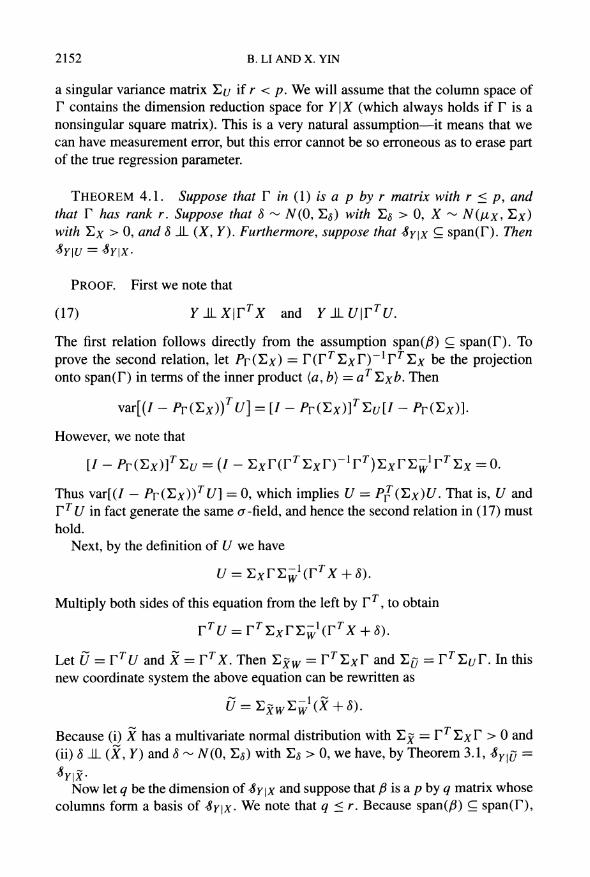
Example 6.1. Still use the model in Example 3.1, but this time, assuming the distribution of X is nonnormal, specified by

Xp =

3Zp<Z>(\\Zp\\)/\\Zp\\, where <i> is the c.d.f. of the standard normal distribution and Zp

~ N(0, Ip). Thus,

conditioning on each line passing through the origin, Xp is uniformly distributed. Note that this is different from a uniform distribution over a ball in Rp, but it is

sufficiently nonnormal to illustrate our point. Figure 2 presents the scatter plots of F versus fifXp, fi\Xp and the scatter plots of F versus fi\Up, fi2Up. We see that, even for p as small as 6, &y\up already very much resembles ?y\xp

for

nonnormal predictors. In fact, we can hardly see any significant difference from

Figure 1, where the invariance law holds exactly.

Although we have only shown the asymptotic version of the invariance law (3) for nonsingular p x p dimensional F, similar extensions can be made for arbitrary T (with r < p), as well as the invariance law (4). Because the development is

completely analogous they will be omitted. Also notice that the assumptions for

Theorem 6.1 impose no restriction on whether X is a continuous random vector; thus the theorem also applies to discrete predictors?so long as its conditions are

satisfied.

7. Estimation procedure and convergence rate. Having established the in

variance laws at the population level, we now turn to the estimation procedure and the associated convergence rate for surrogate dimension reduction. Since we

are no longer concerned with the limiting argument as p ?> oo, we will drop the

subscript p that indicates dimension. Instead the subscripts in (X,-, F/) will now

denote the /th case in the sample. In the classical setting where measurement errors are absent, a dimension re

duction estimator usually takes the following form. Let (X\,Y\),..., (Xn, Yn) be an i.i.d. sample from (X, Y). Let Fxy be the distribution of (X, Y), and FHjxy be

the empirical distribution based on the sample. Let F be the class of all distrib

utions of (X, Y), and # be the class of all p by t matrices. Let T: !F ? $ be a

mapping from !F to $. Most of the existing dimension reduction methods, such as

those described in the Introduction, have the form of such a mapping T, so chosen

that (i) span(7\Fxy)) c Sy\X, and (ii) T(Fn,Xy) = T(FXy) + An, where An is

op(\) or Op(\/^/n) depending on the estimators used. If these two conditions are

satisfied with A? = Op(\/y/n) then we say that T(Fn,xY) is a v^-consistent es

timator of Sy\x\ if, in addition, (i) holds with equality then we say that T(FHyxY) is a v^-exhaustive estimator of $y\x- See Li, Zha and Chiaromonte [18].

The invariance law established in the previous sections tells us that we can ap

ply a classical dimension reduction method to the adjusted surrogate predictor

U\, ...,Un and, if it satisfies (i) and (ii) for estimating ?y\u (or &E(Yk\U))* ^en

it also satisfies these properties for estimating Sy\x (or $E{Yk\X))' Of course, here


o J -1 o J *~

00 . > ?? : . .. . #

* ..

CO - * * ? . CO - - . *

. ! f * . -* n *

*

-4-2024 -4-2024


o o

.

<? - " !" * *L t <? -

I. j* % *

i

-5 0 5 -5 0 5


FlG. 2. Comparison of the original and surrogate dimension reduction spaces for a nonnormal

predictor. Left panels: Y versus fijx (upper) and Y versus fil^X (lower). Right panels: Y versus

pfu (upper) and Y versus fi\\J (lower).

the adjusted surrogate predictor U is not directly observed, because it contains such unknown parameters as E^w and Evy. However, these parameters can be es timated from an auxiliary sample that contains the information about the relation between X and W. As discussed in Fuller [15] and Carroll and Li [3], in practice this auxiliary sample can be available under one of the several scenarios.

1. Representative validation sample. Under this scenario we observe, in addition to (W\ ,Y\),..., (Wn, Yn), a validation sample

(29) (X_,,W_i),...,(X-w,W-m).

We can use this auxiliary sample to estimate Exw and Ew by the method of

moments,

Exw = Em[(X -

X)(W -

W)T], Ew = Em[(W -

W)(W -

W)T],

2162 B.LI AND X.YIN

where Em denotes averaging over the representative validation sample (29). We can then use the estimates Exw and E^ to adjust the surrogate predictor Wt as Vi = Xxw^w wi> a^d

estimate Sy\X by T(Fnm(jY). Here, FnmQY is

FnyUY with U replaced by U; we have added the subscript m to emphasize the

dependence onm.

2. Representative replication sample. In this case we assume that p = r and that F

is known, which, without loss of generality, can be taken as Ip. We have a sep arate sample where the true predictor X; is measured twice with measurement

error. That is,

(30) Wij = y + Xi+8ij, 7 = 1,2, i = -l,...,-m,

where {<50} are i.i.d. N(0, Ea), {X,} are i.i.d. N(0, Ex) and {Stj} AL {(Xt, Yt)}. From the replication sample we can extract information about Exw and E^ as

follows. It is easy to see that, for / = ? 1,...,

? m,

var(W/i -

Wi2) = 2E5, var(Wn + Wi2) = 4EX + 2E3,

from which we deduce

Ys=var(Wn-Wi2)/2,

Ew = var(Wn + Wi2)/4 + var(Wn -

Wi2)/4.

We can then estimate these two variance matrices by substituting in the right hand side the moment estimates of var(Wa + Wt2) and var(Wn

? Wa) derived

from the replication sample (30). Because in this case

ExwEw = Ip

? E<$E^ ,

we adjust the surrogate predictor Wi as Ut = (Ip ?

E^E^ )W(.

A variation of the second sampling scheme appears in Fuller [15], which will be

further discussed in Section 9 in conjunction with the analysis of a data set con

cerning managerial behavior.

Under the above schemes Exw and E^ can be estimated by Exw and E^ at the */m-mtt, as can be easily derived from the central limit theorem. Hence

FnmUY ?

Fn,UY + Op(l/*/m). Meanwhile, by the central limit theorem, we have

Fn,jjy = Fjjy + Op(\/y/n). The dimension reduction estimator T(Fnm qy) can

be decomposed as

T(Fn,m,UY^ (31) = T(FUY) + [T(Fnm0Y)

- T(FnMY)] + [T(FnMY)

- T(FUY)].

Usually the mapping T is sufficiently smooth so that the second term is of order

Op(\/y/m) and the third term is of the order Op(\/*Jn). That is,

(32) T(Fnm0Y) = T(FUY) + Op{l/V^) + 0P(lA/?).


While it is possible to impose a general smoothness condition on T for the above

relation in terms of Hadamard differentiability (Fernholz [14]), it is often simpler to verify (32) directly on an individual basis. The next example will illustrate how

this can be done for a specific dimension reduction estimator.

Example 7.1. Li, Zha and Chiaromonte [18] introduced contour regression (CR) which can be briefly described as follows. Let

(33) Hx(c) = E[(X -

X)(X -

X)TI(\Y -Y\< c)],

in which (X, Y) and (X, Y) are independent random pairs distributed as Fxy, and c > 0 is a cutting point roughly corresponding to the width of a slice in SIR or

? 1/2 ?1/2

SAVE. Let vp-q+\,..., vp be the eigenvectors of Ex Hx^x corresponding to its q smallest eigenvalues. Then, under reasonably mild assumptions,

? 1/2 ?1/2

(34) span(Ex vp,...,T,x vp-q+\) =

<8Y\X'

Thus, the mapping T in this special case is defined by

T(Fxy) = (^i,2vp,..., ^l/2vp-q+i).

For estimation we replace Hx and Ex by their sample estimators,

Hx(c) = (n2) J2 i(Xj - Xt)(Xj - Xt)TI(\Yj -Yt\ <c)], (35) ^ _

Xx = En[(X-X)(X-X)T],

where, in the first equality, N is the index set {(/, j): 1 < j < i < n}. The motivation for introducing contour regression is to overcome the difficulties

encountered by the classical methods. It is well known that if the relation Y\X is

symmetric about the origin then the population version of the SIR matrix is 0, and if E(Y\X) is linear in X then the population version of the pHd matrix is zero. In these cases, or in situations close to these cases, or in a combination of these cases, SIR and pHd tend not to yield accurate estimation of the dimension reduction space. Contour regression does not have this drawback because of the

property (34). In the context of measurement error regression the true predictor X( is to be re

placed by Ut. For illustration, we adopt the first sampling scheme described above. Let E^i and E^2 be the sample estimates of E^ based on the primary sample {W\,...,Wn} and the auxiliary sample {W-\,..., W_m}, respectively. Let Hq(c) be the matrix Hx (c) in (35) with X,-, Xj replaced by ?/, , Uj. Then, it can be easily seen that

^?(c) = ExwE^2//w(c)E;r,2Ewx,

(36) E^7

= ExwEW2EttqEw2Ewx,

2164 B.LI AND X.YIN

where in the first equality Hw (c) is Hx (c) in (35) with X,-, Xj replaced by W,-, Wj. Because Exw and Hw2 are based on the auxiliary sample, they approximate Exw and Ew at the ^/m-ra.te. Because E^i is based on the primary sample, it estimates

Ew at the v^-rate. Consequently, E^ = E^/ + Op(l/^/m) + Op(\/y/n), which

implies

EI1/2 = E"1/2 + Op{\/yfc) + Op(l/Vm).

In the meantime, it can be shown using the central limit theorem for [/-statistics

(see Li, Zha and Chiaromonte [18]) that H\y(c) = Hw(c) + Op(l/^/n), where

Hw(c) is Hx(c) in (33) with X, X replaced by W, W. Hence

HD(c) = i:Xw^wHw(c)^w^wx + Op(\/Jn) + Op(l/yfiR)

(37) = Hv(c) + Op{\/yfc) + Op(l/v^).

Combining (36) and (37) we see that

EI1/2%EI1/2 = E-1/2^E"1/2 + Op(l/Vn) + Op(lA/?).

It follows that the eigenvectors vp-q+\,..., vp of the matrix on the left-hand side

converge to the corresponding eigenvectors of the matrix on the right-hand side,

vp-q+i,..., Vp, at the rate of Op(l/^/n) + Op(l/^/m), and consequently,

X~l/2Vi = Y-l/2Vi + Op{l/yfi) + Op(l/V^).

Thus we have verified the convergence rate expressed in (32).

It is possible to use the general argument above to carry out asymptotic analysis for a surrogate dimension reduction estimator, in which both the rates according to m and n are involved. This can then be used to construct test statistics. But

because of limited space this will be developed in future research. Special cases

are available for SIR and OLS (Carroll and Li [3]) and for pHd (Lue [22]).

8. Simulation studies. As already mentioned, a practical impact of the in

variance law is that it makes all dimension reduction methods accessible to the

measurement error problem, thereby allowing us to tackle the difficult situations

that the classical methods do not handle well. We now demonstrate this point by

applying SIR, pHd and CR to simulated samples from the same model and com

paring their performances. We still use the model in Example 3.1, but this time take F =

Ip. Under this

model E\y = Ex + Es and Exw = Ex. We take an auxiliary sample of size

m = 100. The standard deviations as and ae are taken to be 0.2, 0.4, 0.6. For

the auxiliary sample, we simulate {Wtj : j = 1, 2, / = ? 1,...,

? m} according to

the representative replication scheme described in Section 7. For each of the nine


Table 1

Comparison of different surrogate dimension reduction methods

<re <*8 SIR pHd CR

0.2 1.26 ?0.63 1.35 ?0.56 0.12 ?0.07

0.2 0.4 1.33 ?0.58 1.56 ?0.51 0.16 ?0.09

0.6 1.46 ?0.53 1.57 ?0.46 0.32 ?0.21

0.2 1.44 ?0.57 1.41 ?0.51 0.12 ?0.08

0.4 0.4 1.34 ?0.57 1.5 ?0.5 0.20 ?0.13

0.6 1.36 ?0.59 1.62 ?0.48 0.34 ?0.19

0.2 1.36 ?0.62 1.50 ?0.55 0.13 ?0.08

0.6 0.4 1.44 ?0.53 1.53 ?0.49 0.21 ?0.19

0.6 1.48 ?0.53 1.70 ?0.45 0.32 ?0.18

combinations of the values of ae and a?$, 100 samples of {(Xt, F/)} and {W,-y} are

generated according to the above specifications. The estimation error of a dimension reduction method is measured by the fol

lowing distance between two subspaces of Rp. Let S\ and S2 be subspaces of Rp, and Pi and P2 be the projections onto S\ and S2 with respect to the usual inner

product {a, b) = aTb. We define the (squared) distance between S\ and %2 as

p(*U*2) = \\Pl-Pl\\2,

where || || is the Euclidean matrix norm. The same distance was used in Li, Zha

and Chiaromonte [18], which is similar to the distance used in Xia et al. [25]. For SIR, the response is partitioned into eight slices, each having 50 observa

tions. For CR, the cutting point c is taken to be 0.5, which roughly amounts to

including 12% of the (4^?) = 79800 vectors Ut - Uj corresponding to the low

est increments in the response. The results are presented in Table 1. The symbol a ? b in the last three columns stands for mean and standard error of the distances

p($y\x, &y\x) over the 100 simulated samples. We can see that CR achieves sig nificant improvement over SIR and pHd across all the combinations of as and oe. This is because the regression model (16) contains a symmetric component in the

fti direction, which SIR cannot estimate accurately, and a roughly monotone com

ponent in the ft2 direction, which pHd cannot estimate accurately. In contrast, CR

accurately captures both component. To provide further insights, we use one simulated sample to see the comparison

among different estimators. Figure 3 compares the performance of SIR, pHd and CR in estimating Sy\u (or #y\x)> We see that SIR gives a good estimate for ft2 but a poor estimate for ft\, the opposite of the case for pHd, but CR performs very well in estimating both components.

2166 B.LI AND X.YIN

2 - * o_. . o _ . .

-2-1012 -3-2-10123 -20 2 SIR2 pHdl CR2

o- * o- * o. .

oo- . * eo- * . eo- . *

(O- * . # to - * # <D- * #

-3-2-10123 -2-10 1 2 -3-2-1012 SIR1 pHd2 CR1

FlG. 3. Surrogate dimension reduction by SIR, pHd and CR. Left panels: Y versus the second

(upper) and the first (lower) predictors by SIR. Middle panels: Y versus first (upper) and second (lower) predictors by pHd. Right panels: the second (upper) and the first (lower) predictors by CR.

9. Analysis of a managerial role performance data. In this section we ap

ply surrogate dimension reduction to a role performance data set studied in Warren, White and Fuller [24] and Fuller [15]. To study managerial behavior, n = 98 man

agers of Iowa farmer cooperatives were randomly sampled. The response is the

role performance of a manager. There are four predictors: Xi (knowledge) is the

knowledge of the economic phases of management directed toward profit-making, X2 (value orientation) is the tendency to rationally evaluate means to an economic

end and X3 (role satisfaction) is gratification obtained

(training) is the amount of formal education. The predictors X\, X2 and X3, and the response F are measured with questionnaires filled out by the managers, and contain measurement errors. The amount of formal education, X4, is measured

without error. Through dimension reduction of this data set we wish to see if the

linear assumption in Fuller [15] is reasonable, if there are linear combinations of

the predictors other than those obtained from the linear model that significantly af

fect the role performance, and how different surrogate dimension reduction meth

ods perform and compare in a real data set.

The sampling scheme is a variation of the second one described in Section 7.

A split halves design of the questionnaires yields two observations on each item

with measurement error for each manager, say

(Vn,Vi2), Wn,W/i2).(^31^/32), 1 = 1,...,/!,


where (Vn, V(2) are the two measurements of F; and (Wtj\, W(j2), j = 1,2, 3, are

the two measurements of X/7. The surrogate predictors for Xy, j = 1, 2, 3, are

taken to be the averages Wtj =

(Wij\ + Wij2)/2. Similarly, the surrogate response for Yt is taken to be V( = (Vn + Va)/2. Since the measurement error in F does

not change the regression model, we can treat V as the true response F. As in

Fuller [15], we assume:

1. Vik = Yi + fa, Wijk =

Xij + r)ijk, i = 1,..., n, j

= 1, 2, 3, k = 1, 2, where

{(%ik,mk,m2k,mk)'i = i,...,n,fc = 1,2}

AL{(Yi,Xn,...,XiA):i =

\,...,n}.

2. The random vectors {(?/&> tyn** *7;2ib ^'3j0 :/ = 1,...,?} are i.i.d. 4-dimension

al normal with mean 0 and variance matrix

dmg(aâ2A,a22,a23).

3. {(Xi{,..., Xi4): n = 1,..., n] are i.i.d. N(/xx, Ex).

From these assumptions it is easy to see that, for j = 1,..., 4 and i = 1,..., n,

Wtj ?

Xij +8ij, where

{(?n,...,?i4):i =

l,...,n}JL{(Xn,...,XI-4,r?):i =

l,.-.,n}.

and {(8n,..., 8^): i = 1,..., n) are i.i.d. mean 0 and variance matrix

E5 = diag(a| j, <t522, a|3, 0), o/

, = \ var( Wy i

- Wy2),

(38) '

7 =

1,2,3.

Thus, at the population level, our measurement error model can be summarized as

W = X + 8, 8 AL (X, V), 8- N(0, E<0, X - N(fix, Ex),

where E?$ is given by (38). Note that, unlike in Fuller [15], no assumption is im

posed on the relation between F and X.

The measurement error variance E$ is estimated using the moment estimator of

(38) based on the sample {(Wtju Wij2): i = 1,..., 98, j = 1,..., 3}, as

% = diag(0.0203, 0.0438, 0.0180, 0).

The variance matrix E^ of W( = (Wn,..., W^)7 is estimated from the sample {W/:i = l,...,98}as

/ 0.0520 0.0280 0.0044 0.0192 \ 0.0280 0.1212 -0.0063 0.0353

0.0044 -0.0063 0.0901 -0.0066 *

V 0.0192 0.0353 -0.0066 0.0946 /

The correction coefficients ExwE^,1 are then estimated by I4

- EÊ^1, and the

surrogate predictor Wt corrected as [/,- = (I4 ?

EÊ^1)^-.

2168 B.LI AND X.YIN

-* Tt o

"j ~?

| d 1

~ I

II I co J CO J 6 1 d 1 I

S H # ^ \ * ? 1

* %

_ _

? 1 ' . > 1

* PJ q J .. ?

? 1 %# ? I

* * *

CM ^ * CM %

d i d H I II*

-1-1-1-T-1-' \-1-1-\-1-1-'

-2-1012 -3-2-1012

SIR1 CR1

FlG. 4. Scatter plots of role performance versus the first predictor by SIR (left) and versus the first

predictor by CR (right).

We apply SIR and contour regression to the surrogate regression problem of V/ versus ?/,-. As in Fuller [15], a portion of the data (55 out of 98 subjects) will be

presented. For SIR, the responses of 55 subjects are divided into five slices, each

having 11 subjects. For CR, the cutting point c is taken to be 0.1, which amounts to

including 552 of the (525) = 1485 (roughly 37%) differences ?/,- ?

Uj corresponding to the lowest increments | F/

? Yj \ of the response. In fact, varying the number of

slices for SIR or the cutting point c for CR within a reasonable range does not

seem to have a serious effect on their performance.

Figure 4 shows the scatter plots of F versus the first predictors calculated by SIR

(left) and CR (right). None of the scatter plots of F versus the second predictors by SIR and CR shows any discernible pattern, and so they are not presented. Because

there is no U-shaped component in the data, the accuracy of SIR and CR are

comparable. These plots show that the linear model postulated in Warren, White

and Fuller [24] and Fuller [15] does fit this data, and there do not appear to be other

linear combinations of the predictors that significantly affect the role performance. The directions obtained from CR, SIR, and that using the maximum likelihood

estimator for a linear model, are presented in Table 2 (the vectors are rescaled to

have lengths 1).

Table 2

$1 $2 03 04

Fuller [15] 0.881 0.365 0.286 0.098 SIR (Carroll and Li) 0.952 0.219 0.187 0.102

CR 0.935 0.291 0.126 0.159


Note that SIR, as applied to the adjusted surrogate predictor U, is the estimator

proposed in Carroll and Li [3]. We can see that for this data set the three meth ods are more or less consistent, though CR gives more weight to past education

than the other methods. Of course, the significance of these parameters should be

determined by a formal test based on the relevant asymptotic distributions. Such

asymptotic results are available for pHd and SIR, and are under development for CR.

APPENDIX

Proof of Lemma 5.1. Note that the conditions for equality (9) are still sat

isfied. Multiply both sides of (9) by h(Y) and then take expectation, to obtain

ElhiY^v*^'2*7^1 = E[h(Y)eitTy*\Y}e^tT^*t. To prove the first assertion, suppose there is a V3* such that V3* JL (V*

? V3*, V2*)

and E\h(Y)\V*, V3*] =

E[h(Y)\Vf]. Then

E(h(Y)eitTv*) = E(E[h(Y)\V*, V^^'ê^êlt^) =

E(E[h(Y)\V3*]eit^v*-vêi'2v2eitfv^ =

E(ei'^v*-vêi'2v2*)E(h(Y)ei'Iv^.

Follow the steps that lead to (13) in the proof of Lemma 3.1 to obtain

E(h(Y)eitTu*) =

E(h(Y)eit'u*)e~tû2t2.

The equation can be rewritten as

E(E[h(Y)\U*]eifTu*) = E(E[h(Y)\Uêitû*)e~tû2t2.

Because ?/* _LL U%, the right-hand side is

E(E[h(Y)\U^]eû*+it2u2) =

E(E[h(Y)\UtytTu*). It follows that

E({E[h(Y)\U*] -

E[h(Y)\Uf]}eitTu*) = 0

for all t. In other words, the Fourier transform of E[h(Y)\U*] -

E[h(Y)\Uf] is zero. Thus E[h(Y)\U*]

- E[h(Y)\Uf]

= 0 almost surely. The proof of the second assertion will be omitted.

Proof of Lemma 6.1. 1. That (22) implies (pp(t; ftp) -+ co(t) is well p p

known. Now suppose c/)p(t; ftp) -* co(t). Then \(pp(t; ftp)\2

-+ \co(t)\2. Because both <pp(t; ftp) and \(/)p(t; ftp)\2 are bounded, (22) holds.

2170 B.LI AND X.YIN

2. Because Rp AL Sp\Tp, fip, we have

= E(eifTR*\T*)E(eiuTs*\T*)

+ [E(eitTRP\Tp,fip)E(eiuTsP\Tp,fip)-E(eitT^\T*)E(ei^

+ [E(eitTR\iuTs*\T*)-E(eitTRPeiuTsP\Tp,fip)l

Because (Rp, Sp, Tp)\fip -> (/?*, S*, T*) w.i.p., the last two terms on the right

hand side are op (1). Hence the left-hand side equals the first term on the right-hand side because the former is a nonrandom quantity independent of p.

Proof of Lemma 6.2. It suffices to show that, if Ap and Bp are regu lar sequences of random vectors in R^ such that Ap JL Bp and E(Ap)

= 0,

E(Bp) = 0, then

p~~xATpBp = op(\). If this is true then we can take Ap

= Xp, Up,

or E^/E^ Xp and Bp =

Xp,Up, or EfyE^Xp to prove the desired equality.

By Chebyshev's inequality,

(39) P(p-l\ATpBp\ >e)< -^E(ATpBp)2.

The expectation on the right-hand side is

E(itAiPBp) = ?X>(4VW

\i = l / 1 = 1 y = l

p p

= EEE^7E5,0-<||EA||F||E5||F,

i = l 7 = 1

where the inequality is from the Cauchy-Schwarz inequality. By assumption, ||Ea||f = o(p) and ||E#|| = o(p). So the right-hand side of (39) converges to

0 as p -> oo. Hence ATpBp

= op(\). D

Acknowledgments. We are grateful to two referees and an Associate Edi

tor who, along with other insightful comments, suggested we consider the situa

tions where the predictor and measurement error have non-Gaussian distributions, which led to the development in Section 6.

REFERENCES

[1] BILLINGSLEY, P. (1968). Convergence of Probability Measures. Wiley, New York. MR0233396

[2] CARROLL, R. J. (1989). Covariance analysis in generalized linear measurement error models.

Stat. Med. 8 1075-1093.


[3] Carroll, R. J. and Li, K.-C. (1992). Measurement error regression with unknown link:

Dimension reduction and data visualization. J. Amer. Statist. Assoc. 87 1040-1050.

MR1209565 [4] CARROLL, R. J., RUPPERT, D. and STEFANSKI, L. A. (1995). Measurement Error in Nonlin

ear Models. Chapman and Hall, London. MR 1630517

[5] Carroll, R. J. and Stefanski, L. A. (1990). Approximate quasi-likelihood estimation in

models with surrogate predictors. J. Amer. Statist. Assoc. 85 652-663. MR1138349

[6] COOK, R. D. (1994). Using dimension-reduction subspaces to identify important inputs in

models of physical systems. In ASA Proc. Section on Physical and Engineering Sciences

18-25. Amer. Statist. Assoc, Alexandria, VA.

[7] COOK, R. D. (1998). Regression Graphics: Ideas for Studying Regressions Through Graphics.

Wiley, New York. MR 1645673 [8] COOK, R. D. (2007). Fisher lecture: Dimension reduction in regression. Statist. Sci. 22 1-26.

[9] COOK, R. D. and Li, B. (2002). Dimension reduction for the conditional mean in regression. Ann. Statist. 30 455-474. MR 1902895

[10] COOK, R. D. and Li, B. (2004). Determining the dimension of iterative Hessian transforma

tion. Ann. Statist. 32 2501-2531. MR2153993

[11] COOK, R. D. and Weisberg, S. (1991). Discussion of "Sliced inverse regression for dimen

sion reduction," by K.-C. Li. J. Amer. Statist. Assoc. 86 328-332.

[12] Diaconis, P. and Freedman, D. (1984). Asymptotics of graphical projection pursuit. Ann.

Statist. 12 793-815. MR0751274 [13] Duan, N. and Ll, K.-C. (1991). Slicing regression: A link-free regression method. Ann. Sta

tist. 19 505-530. MR1105834 [14] FERNHOLZ, L. T. (1983). von Mises Calculus for Statistical Functionals. Lecture Notes in

Statist. 19. Springer, New York. MR0713611

[15] FULLER, W. A. (1987). Measurement Error Models. Wiley, New York. MR0898653

[16] Fung, W. K., He, X., Liu, L. and Shi, R (2002). Dimension reduction based on canonical

correlation. Statist. Sinica 12 1093-1113. MR 1947065

[17] Hall, R and Li, K.-C. (1993). On almost linearity of low-dimensional projections from high dimensional data. Ann. Statist. 21 867-889. MR 1232523

[18] Li, B., ZHA, H. and Chiaromonte, F. (2005). Contour regression: A general approach to

dimension reduction. Ann. Statist. 33 1580-1616. MR2166556

[19] Li, K.-C. (1991). Sliced inverse regression for dimension reduction (with discussion). J. Amer.

Statist. Assoc. 86 316-342. MR1137117

[20] Li, K.-C. (1992). On principal Hessian directions for data visualization and dimension re

duction: Another application of Stein's lemma. J. Amer. Statist. Assoc. 87 1025-1039.

MR 1209564 [21] Li, K.-C. and Duan, N. (1989). Regression analysis under link violation. Ann. Statist. 17

1009-1052. MR1015136 [22] LUE, H.-H. (2004). Principal Hessian directions for regression with measurement error. Bio

metrika 91 409-423. MR2081310 [23] Pepe, M. S. and Fleming, T. R. (1991). A nonparametric method for dealing with mismea

sured covariate data. J. Amer. Statist. Assoc. 86 108-113. MR1137103

[24] Warren, R. D., White, J. K. and Fuller, W. A. (1974). An errors-in-variables analysis of managerial role performance. J. Amer. Statist. Assoc. 69 886-893.

[25] XlA, Y., TONG, H., Li, W. K. and Zhu, L.-X. (2002). An adaptive estimation of dimension

reduction space. J. R. Stat. Soc. Ser. B Stat. Methodol. 64 363-410. MR1924297

[26] Yin, X. and Cook, R. D. (2002). Dimension reduction for the conditional &-th moment in

regression. J. R. Stat. Soc. Ser. B Stat. Methodol. 64 159-175. MR 1904698

[27] Yin, X. and Cook, R. D. (2003). Estimating central subspaces via inverse third moments.

Biometrika 90 113-125. MR 1966554

2172 B.LI AND X.YIN

[28] Yin, X. and COOK, R. D. (2004). Dimension reduction via marginal fourth moments in re

gression. /. Comput. Graph. Statist. 13 554-570. MR2087714

Department of Statistics

326 Thomas Building

Pennsylvania State University

University Park, Pennsylvania 16802

USA E-mail: [email protected]

Department of Statistics

Franklin College

107 Statistics Building

University of Georgia

Athens, Georgia 30602-1952

USA E-MAIL: [email protected]

On Surrogate Dimension Reduction for Measurement Error ...

Documents

Transcript of On Surrogate Dimension Reduction for Measurement Error ...