On steady columnar vortices under local compression · On steady columnar vortices under local...

J. Fluid Mech. (1995), vol. 299, p p . 367-388 Copyright @ 1995 Cambridge University Press

367

On steady columnar vortices under local compression

By ROBERTO VERZICCO1 JAVIER JIMENEZ2 AND PAOLO O R L A N D I l

Universita di Roma “La Sapienza” Dipartimento di Meccanica e Aeronautica, via Eudossiana 18, 00184 Roma, Italy

2School of Aeronautics, U. PolitCcnica, P1. Cardenal Cisneros 3,28040 Madrid, Spain

(Received 26 January 1995 and in revised form 11 May 1995)

Numerical simulations are presented of the long time behaviour of viscous columnar vortices subject to non-uniform axial stretching. The relevant result is that the vortices reach a steady state even when the axial average of the strain is zero, such that they are being compressed during half of their extent. The structure of the flow is analysed and shown to range from local Burgers equilibrium to massive separation. For an intermediate range of Reynolds numbers the vortices are more or less uniform and compact, and it is suggested that this condition is related to the strong vortices observed in turbulent flows. The reason for the survival of the vortices under compression is traced to induced axial pressure gradients and to the viscous cancellation of outgoing vorticity. Theoretical analyses of the linear Burgers’ regime and of the onset of separation are presented and compared to the numerical experiments. The results are related to the observation of intermittency in turbulence, and shown to be consistent both with the observed scaling of vortex diameter, and with the lack of intermittency of the velocity signal.

1. Introduction It has been recognized in the last few years that strong coherent elongated vortices

are present among the small scales of many turbulent flows (Siggia 1981; Kerr 1985; Hosokawa & Yamamoto 1990; She, Jackson & Orszag 1990; Ruetsch & Maxey 1991 ; Vincent & Meneguzzi 1991), and that they are important in the characterization of the intermittent properties of high Reynolds number turbulence. It is generally agreed that they are formed by stretching of pre-existing vorticity, and it has been shown from the correlation of numerical simulations at several Reynolds numbers (Jiminez et al. 1993) that their radii are of the order of the Kolmogorov length and scale with it. It has also been shown that, along a considerable fraction of their length, they are near the Burgers limit, at which axial stretching is in equilibrium with viscous diffusion, and that the stretching itself is of the order of the mean square vorticity of the flow m’ (Jimhnez & Wray 1994~). This is also the magnitude of the average strain in the bulk of the flow. The length of the vortices is known to be large, comparable to the integral scale of the flow O ( 9 ) .

A first tempting idea was that elongated vortices in turbulence were just the result of uniformly stretched vorticity, however it was pointed out in (Jiminez et aE. 1993) that this strain, if it were to hold consistently along the length of vortices, would be

368 R. Verzicco, J. Jimbnez and P. Orlandi

inconsistent with the measurements of turbulent velocity, since the velocity difference between the two ends of the vortex would be O(o’3’) m O(u’ReJ, where ReA = u’l/v is the Reynolds number based on the Taylor microscale, and u’ is the mean square velocity. No such large velocity differences have been observed in turbulent flows, and the probability distribution of the velocity is known to be largely free of Reynolds number effects (Anselmet et al. 1984). A second unexplained observation was that the average circulation I‘ of the vortices increased with the Reynolds number as

r / v - Re!, (1.1)

with a in the range 0.3-0.5 (Jimenez et al. 1993). Both problems were addressed in Jimenez & Wray (19944 It was first shown, by direct measurement of the numerical simulation fields, that the stretching along the vortex axes was not uniform, and that a substantial percentage of the points were under axial compression, rather than stretching.

The result that strong vortices would survive under local compression was unex- pected, and it was conjectured that it was due to the presence of axial pressure waves that smooth the effect of the local axial strain and help to make the cores uniform. It was also observed in that paper that the relation in (1.1) corresponds to a fixed ratio between the celerity of the waves and the velocities induced by the driving strain, which were assumed to be of O(u’).

The present paper is an attempt to verify those conjectures and, in particular, to determine the conditions under which more or less uniform vortex filaments can form under the action of a non-uniform strain whose spatial average is zero. We will show, by direct numerical simulation of vortices subject to different strain laws, that this is possible and that it is mediated by axial waves damped by viscosity. It will turn out, however, that the naive identification of the governing parameter for vortex survival, as the ratio of wave celerity to axial velocity, is incorrect. The right parameter will be identified, both theoretically and numerically.

That axial waves make uniform vortex cores with initially variable cross-sections was first proposed by Moore & Saffman (1972), who used the assumption to jus- tify the use of uniform core size in models for the motion of vortex filaments of arbitrary shape. The particular case of unstrained viscous straight filaments was studied recently by Melander & Hussain (1994) who refer to the axial waves by the name of ‘core dynamics’. The waves themselves were known to Kelvin (1880) in the linear limit, and several model equations for their nonlinear behaviour have been proposed since then (Lundgren & Ashurst 1989; Leonard 1994). In most cases, the models are inviscid, since the waves are inertial and do not depend on viscosity. Caflisch, Li & Shelley (1993) have computed numerically the nonlinear behaviour of the waves in an inviscid vortex with a very singular initial vorticity distribution.

The study of vortices under variable strain has been generally connected to vortex breakdown (Leibovich 1978). That problem is only loosely connected to ours, since most of the external pressure gradient is due in that case to the deformation of the vortex, while in ours it is imposed as a boundary condition. It was realized early that breakdown depends on the existence of axial stationary waves, which can only occur if the wave celerity is at least as large as the velocity of the incoming flow (Benjamin 1962). This is equivalent to the naive theory used above to rationalize the scaling of the intensity of the ‘worms’. More recently Brown & L6pez (1990) have studied a case closer to ours, in which breakdown is artificially triggered by confinement in a rotating vessel, and have also found the naive theory

Columnar vortices under local compression 369

to be inapplicable. As in the case of unstrained vortices, most theoretical models are inviscid, but the effect of Reynolds number has been investigated numerically (Beran & Culick 1992).

In this paper we are mainly interested in viscous vortices, and in the effect of Reynolds number. The equations of motion, the numerical method and the run parameters are described in §2. After a short description of preliminary results on unstrained vortices and on vortices subject to uniform strain, the numerical experiments using steady non-uniform strain are described in 93. The results are then discussed and related to the observations in turbulent flows.

2. Numerical set-up 2.1. Integration scheme

The simulation code solves the initial value problem for the incompressible viscous Navier-Stokes equations. It is described in detail in Verzicco & Orlandi (1993) and only the main points are summarized here. The equations are written in primitive variables in cylindrical coordinates, and discretized using central second-order finite differences on a staggered grid, with the velocity on the faces and the pressure at the centres of the cells. The scheme conserves energy in the inviscid limit. While the code is capable of dealing with fully three-dimensional flows, most of the simulations in this paper are axisymmetric.

The resulting system of equations is advanced in time by a fractional-step method. The first sub-step generates a non-solenoidal velocity field using a third-order explicit Runge-Kutta scheme for the nonlinear terms (A. Wray, personal communication) and an implicit Crank-Nicholson for the viscous ones. In the second sub-step the result is projected onto the final solenoidal velocity. The necessary Poisson equation is solved using trigonometric expansions, and yields a velocity field which is divergence-free to within the round-off error.

Since the coordinate system is singular at r = 0, the radial component of the momentum equation is written in terms of qr = ru,., instead of u,. Because of the staggered mesh, this is the only quantity that has to be computed at r = 0, and its definition forces it to vanish there.

The original code was modified to treat flows subject to an external axisymmetric irrotational non-uniform strain, which is considered as given. The full velocity field is formed by the forcing flow plus a perturbation connected to the vortex, and only the perturbation velocity is allowed to evolve. If the driving strain is chosen as a solution of the Euler equations, the perturbation velocity still satisfies the full Navier- Stokes equations, although the strain might correspond to fairly artificial pressure and velocity distributions far from the axis. In a real flow, the irrotational region would not be infinite, and the driving strain would be generated by other vortices or by the presence of walls.

Since it has been observed in the introduction that significant strain fields with large coherence lengths imply unrealistic velocity differences, we will be mostly interested in driving strains which are periodic in the axial direction, and which have zero mean. This is an extreme case of variable axial stretching, which compresses a vortex along half of its length, and stretches it along the other half.

Let r and x be the radial and axial coordinates and us and us the driving velocity components in those directions. The requirement that they be solenoidal and

370

irrotational implies a stream function tp, such that

R. Verzicco, J. JimCnez and P. Orlandi

The elementary non-singular periodic solutions are

S y ( r , x) = - - r I l ( p r ) sin(px),

P2 where S is the maximum axial strain at the axis, p = 2n/L is the wavenumber, L the wavelength, and 11 the first-order modified Bessel function of the first kind.

In most of our simulations, this will be the driving strain, and L will be the length of the computational domain, which acts also as a periodicity wavelength for the whole flow.

The axial strain corresponding to (2.2) is

where I. is again a modified Bessel function of the zeroth order and first kind. Note that, when r << L near the axis, lo(br) = 1 + O(pr)*, and the driving flow is approximated by s(0, x ) = -S cos(Px) and us = -s(O, x ) r / 2 , which behaves locally as an axial strain with non-uniform strength along the axis, and zero mean. In fact, as f i -+ 0, the velocities induced by equation (2.2) tend to us = Sx and v, = -Sr /2 , which are those of a uniform axial strain S .

Far from the axis, both the velocities and the strain generated by (2.2) grow exponentially as exp(pr). While this growth is responsible for some numerical problems which will be discussed below, it is no more surprising than that the radial velocity due to a uniform strain should grow linearly with the radius. In real flows, a periodic strain could be generated by an array of vortex rings of alternating signs, at some large but finite distance from the axis. In our model we are assuming that those rings do not evolve with the flow but that they drive the evolution of a straight vortex lying along their common axis.

2.2. Flow parameters The results of our simulations are presented normalized with the vortex circulation r and with the axial length of the domain L. There are two dimensionless parameters: a Reynolds number based on the circulation, Rer = r/v, where v the kinematic viscosity, and another one related to the driving strain, ReL = S L 2 / v . The first one characterizes the azimuthal flow generated by the vortex, which has typical velocities O(r /a ) at some radius a, such that a typical Reynolds number is a ( r / a ) / v = Rer. The second one is related to the axial flow induced by the driving strain, which is O ( S ) with a coherence length O(L), and typical velocities O(SL).

The character of the flow depends on the relative magnitude of these two parameters. A useful combination is obtained if the characteristic radius a is taken to be of the order of the viscous length based on the strain, a = ( v / S ) ’ / ~ . The ratio of azimuthal to axial velocities, a Rossby number, is then

This ratio is related to the helical angle of the velocities within the vortex.


Case 1 2 3 4 5 6 7 8 9 10 11 12 13 14 15 16 17 18 19 20 21 22 23 24 25 26 27 28 29 30 31 32

S Rer 0.0980 12.5 0.0980 25 0.0980 43.2 0.0980 88.2 0.0980 200 0.2000 12.5 0.2000 25 0.2000 40 0.2000 56.4 0.2000 100 0.2000 150 0.2000 200 0.3947 12.5 0.3947 25 0.3947 37.5 0.3947 50 0.3947 75 0.3947 100 0.3947 150 0.3947 200 0.3947 300 0.3947 400 0.7895 12.5 0.7895 25 0.7895 50 0.7895 75 0.7895 100 0.7895 200 0.7895 300 0.7895 400 0.1753 50 0.5919 50

Ken 44.1 86.4

152.4 311.2 705.6 90

180 288 406 720

1080 1440 177.5 355 532.8 710.3

1065.6 1420.9 2131.4 2841.8 4262.8 5683.7 355 710.6

1421.1 2131.6 2842.2 5684.4 8526.6

11368.8 710.2 710.2

Rer /Re:”

1.882 2.689 3.499 5.000 7.529 1.317 1.863 2.357 2.800 3.726 4.564 5.270 0.938 1.327 1.624 1.876 2.297 2.652 3.249 3.751 4.595 5.305 0.663 0.937 1.326 1.624 1.875 2.652 3.248 3.751 1.876 1.876

Rer / 3.538 5.655 8.087

13.016 22.465 2.789 4.427 6.057 7.616

11.157 14.620 17.711 2.224 3.530 4.625 5.604 7.343 8.895

11.656 14.120 18.502 22.414

1.765 2.801 4.447 5.827 7.059

11.206 14.685 17.789 5.604 5.604

TABLE 1. Run parameters of the cases with steady non-uniform strain.

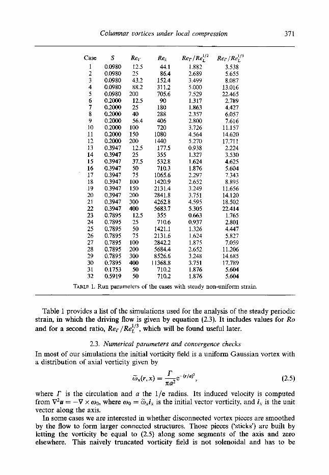
Table 1 provides a list of the simulations used for the analysis of the steady periodic strain, in which the driving flow is given by equation (2.3). It includes values for Ro and for a second ratio, Rer/ReL’3, which will be found useful later.

2.3. Numerical parameters and convergence checks In most of our simulations the initial vorticity field is a uniform Gaussian vortex with a distribution of axial vorticity given by

r GJ~, x) = -e+/U)*, na2 (2-5)

where r is the circulation and a the l /e radius. Its induced velocity is computed from V2u = -V x 00, where 00 = GXix is the initial vector vorticity, and i, is the unit vector along the axis.

In some cases we are interested in whether disconnected vortex pieces are smoothed by the flow to form larger connected structures. Those pieces (‘sticks’) are built by letting the vorticity be equal to (2.5) along some segments of the axis and zero elsewhere. This naively truncated vorticity field is not solenoidal and has to be

372 R. Verzicco, J . Jirndnez and P. Orlandi

6.5 7

2 -

0, r T 6.0 1 -

5 . 5 .I

(b)

.................................................. . . . . . . . . . --

............................................

completed before a velocity field can be computed. Let oT be the truncated vorticity. A straightforward variational analysis shows that a solenoidal field can be constructed by adding the gradient of a scalar 00 = O T + V ~ , where V 2 4 = -VWT. This procedure results in a minimum enstrophy for the difference between the original and projected fields.?

The strain field given in (2.3) is periodic in x with zero spatial average, and its velocity field is also periodic. The initial condition is given by the driving velocity plus the velocity induced by the initial vortex.

The computational domain is periodic in x, but is truncated radially at an artificial boundary R, where the velocity field is forced to be equal to the irrotational driving velocity. It would of course be desirable to have this outer boundary as far as possible from the axis, but the Bessel functions in the driving field (2.3) grow exponentially with r , making it impossible to extend the simulation to very large radii, because of numerical stability constraints.

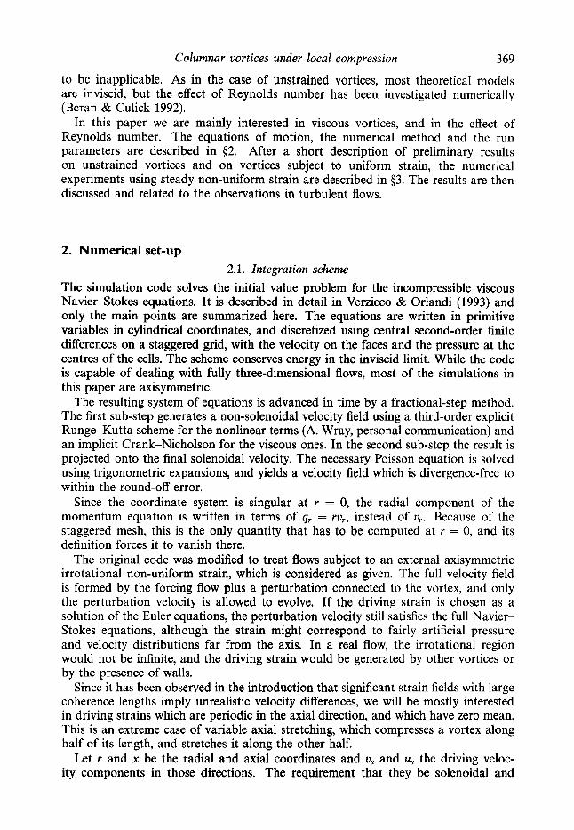
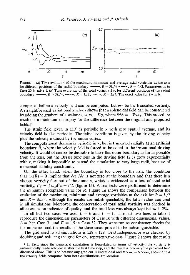
On the other hand, when the boundary is too close to the axis, the condition that o,(R) = 0 implies that do,/dr is not zero at the boundary and that there is a viscous vorticity flux out of the domain, which is evidenced as a loss of total axial vorticity, rT = J w,d3x = r L (figure lb) . A few tests were performed to determine the minimum acceptable value for R. Figure l a shows the comparison between the evolution of the maximum, minimum and average vorticities at the axis for R = L/2 and R = 3L/4. Although the results are indistinguishable, the latter value was used in all simulations. Moreover, the conservation of total axial vorticity was checked in all cases, as an indicator of quality, and the total loss was always kept below 1-2%.

In all but two cases we used L = 6 and r = 1. The last two lines in table 1 reproduce the dimensionless parameters of Case 16 with different dimensional values, L = 9 in Case 31 and r = 1.5 in Case 32. They were run as consistency checks for the numerics, and the results of the three cases proved to be indistinguishable.

The grid used in all simulations is 128 x 128. Grid independence was checked by doubling and reducing the grid for one representative case. Figure 2 shows the results

t In fact, since the numerical simulation is formulated in terms of velocity, the vorticity is automatically made solenoidal after the first time step, and the result is precisely the projected field discussed above. This is so because any gradient is irrotational and V x wo = V x W T , showing that the velocity fields computed from both distributions are identical.


2

% 1

0 50 100 150 200 t

FIGURE 2. Time evolution of the maximum, minimum and mean axial vorticities at the axis for different numerical resolutions: .......-, 96 x 96 grid; - , 128 x 128; - - - - ,256 x 256. Parameters as for Case 22 in table 1.

0 20 40 60 t

FIGURE 3. Time evolution of the maximum axial vorticity at the axis for different initial uniform vortex cores: -, a = 0.25; ---, a = 0.5; ----, a = 1. Conditions as in Case 20 in table 1.

obtained for the Case 22 using the standard resolution, together with those obtained from 96 x 96 and 256 x 256 grids. While there are some differences between the two smallest grids, the two largest ones agree within the precision of the plot.

The different cases were followed until they converged to a steady state, and some tests were run to ensure the independence of this final state from the initial conditions. The typical initial condition is given by equation (2.4) with a = 0.5. For Case 20 the simulation was repeated with initial radii a = 1 and a = 0.25. Time histories for the maximum vorticity at the axis in the three cases are shown in figure 3, and converge to the same value. Note that the three initial conditions were chosen so that the maximum initial vorticities were below, above and comparable to the final value. In addition, another test was run in which the initial condition was taken as four short equidistant ‘sticks’, each of length L/6, generated as described above. The final state was again indistinguishable from those starting from uniform vortices.

374

3. Results 3.1. Relinking of unstruined vortices

Before getting into the discussion of the results for variable driving strains, it is important to summarize the mechanism by which axial waves develop in vortices with variable cross-sections. Consider a straight vortex with constant circulation r , whose core radius R(x) varies along its axis, and let uo(x) - r / R ( x ) be the order of magnitude of tangential velocity at the core boundary. Assume that the flow is otherwise at rest, and denote by pa the pressure at infinity, far from the axis. The pressure at the vortex axis will be approximately p(x) = pa - pui(x), where p is the density of the fluid. It is clear from those relations that the pressure at the axis is low where the core is narrow and high where it is wide. This generates a pressure gradient that drives an axial flow from wide to narrow regions, and which tends to counteract the deformation of the vortex. As fluid flows into the narrow sections, they tend to become wider, and vice versa.

The result is an axial wave that was already known to Kelvin (1880), whose celerity is c w O(u0). If the flow were inviscid, there would be no obvious mechanism to damp these waves, although they are known to be dispersive, and any initial condition would probably degenerate into a disorganized wave train, in the same way as gravity waves in water. Moreover, their nonlinear evolution is thought to include vortex ‘shocks’ and instabilities (Lundgren & Ashurst 1989), which could also be responsible for the decay of initial perturbations. Moore & Saffman (1972) had apparently some of these mechanisms in mind when they proposed axial waves as a means for the homogenization of vortex cross-sections (private communication).

In viscous flows at moderate Reynolds numbers, waves of small amplitude are known to be damped by viscosity and, in a finite time, the vortex decays into a uniform core (Melander & Hussain 1994). In the early stages of the present work, we were able to demonstrate a more extreme example of the same phenomenon, in which a uniform core forms from several separate vortex pieces, or ‘sticks’, which can be considered as limiting cases of very narrow and wide core distortions. This ‘relinking’ gives some support to one of the possible models for the formation of long vortices in three-dimensional turbulent flows, by which short vortex pieces would be formed by local stretching and would then relink into longer structures by means of axial waves (Jimenez et al. 1993; Jimbnez & Wray 1994b).

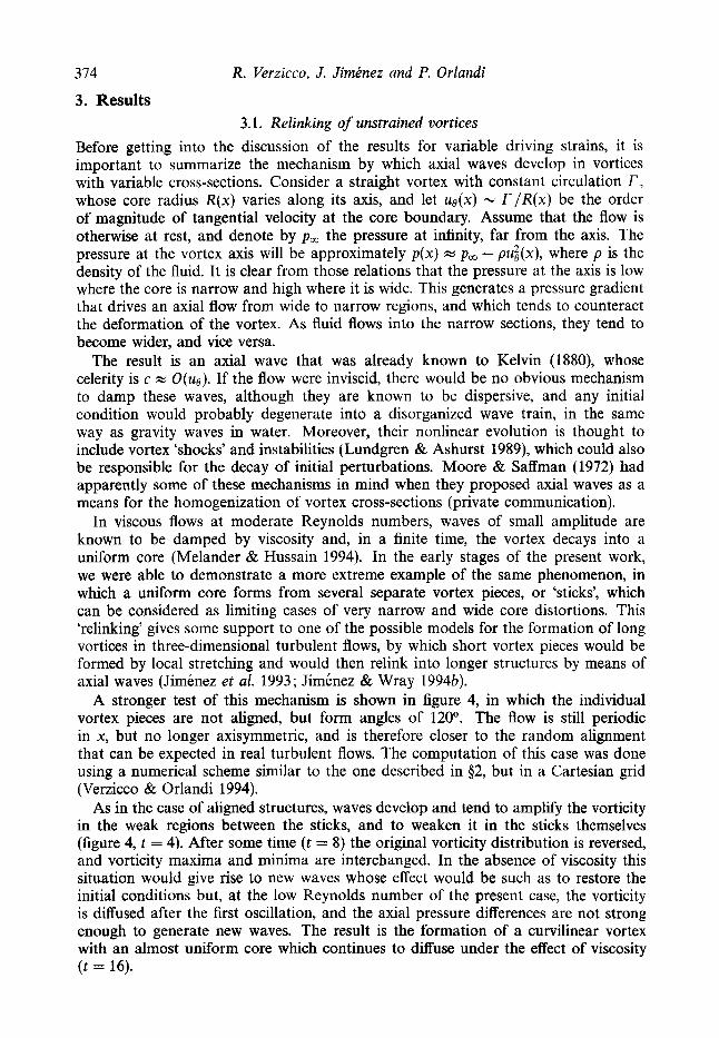
A stronger test of this mechanism is shown in figure 4, in which the individual vortex pieces are not aligned, but form angles of 120”. The flow is still periodic in x, but no longer axisymmetric, and is therefore closer to the random alignment that can be expected in real turbulent flows. The computation of this case was done using a numerical scheme similar to the one described in $2, but in a Cartesian grid (Verzicco & Orlandi 1994).

As in the case of aligned structures, waves develop and tend to amplify the vorticity in the weak regions between the sticks, and to weaken it in the sticks themselves (figure 4, t = 4). After some time ( t = 8) the original vorticity distribution is reversed, and vorticity maxima and minima are interchanged. In the absence of viscosity this situation would give rise to new waves whose effect would be such as to restore the initial conditions but, at the low Reynolds number of the present case, the vorticity is diffused after the first oscillation, and the axial pressure differences are not strong enough to generate new waves. The result is the formation of a curvilinear vortex with an almost uniform core which continues to diffuse under the effect of viscosity (t = 16).

R. Verzicco, J. Jiminez and P. Orlandi


t = O t = 2 t = 4

t = 6 t = 8 t = 16

FIGURE 4. Iso-surfaces of vorticity magnitude for angled sticks at Rer = 200. Iso-surface is always drawn at IwI = 0.6 I w,,,(t) I. The initial angle between stick axes is 120" (64 x 64 x 64 grid).

t = O , Lx=4. t = 8 , Lx=6.61. t = 16, Lx=10.93.

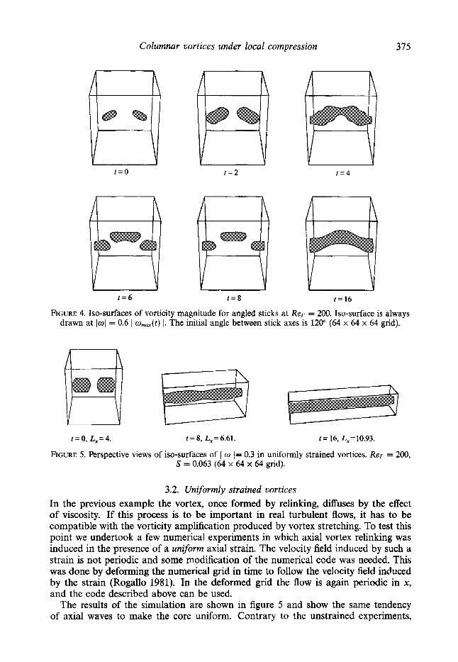
FIGURE 5. Perspective views of iso-surfaces of I w I= 0.3 in uniformly strained vortices. Rer = 200, S = 0.063 (64 x 64 x 64 grid).

3.2. Uniformly strained vortices In the previous example the vortex, once formed by relinking, diffuses by the effect of viscosity. If this process is to be important in real turbulent flows, it has to be compatible with the vorticity amplification produced by vortex stretching. To test this point we undertook a few numerical experiments in which axial vortex relinking was induced in the presence of a uniform axial strain. The velocity field induced by such a strain is not periodic and some modification of the numerical code was needed. This was done by deforming the numerical grid in time to follow the velocity field induced by the strain (Rogallo 1981). In the deformed grid the flow is again periodic in x, and the code described above can be used.

The results of the simulation are shown in figure 5 and show the same tendency of axial waves to make the core uniform. Contrary to the unstrained experiments,

376 R. Verzicco, J . Jirninez and P. Orlandi

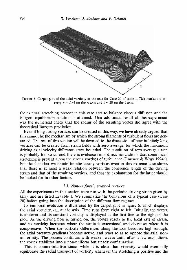
FIGURE 6. Carpet plot of the axial vorticity at the axis for Case 20 of table 1. Tick marks are at every x = L/4 on the x-axis and t = 20 on the t-axis.

the external stretching present in this case acts to balance viscous diffusion and the Burgers equilibrium solution is attained. One additional result of this experiment was the numerical check that the radius of the resulting vortex did agree with the theoretical Burgers prediction.

Even if long strong vortices can be created in this way, we have already argued that this cannot be the mechanism by which the strong filaments of turbulent flows are generated. The rest of this section will be devoted to the discussion of how infinitely long vortices can be created from strain fields with zero average, for which the maximum driving axial velocity difference stays bounded. The condition of zero average strain is probably too strict, and there is evidence from direct simulations that some mean stretching is present along the strong vortices of turbulence (Jimtnez & Wray 1994a), but the fact that we obtain infinite steady vortices even in this extreme case shows that there is at most a weak relation between the coherence length of the driving strain and that of the resulting vortices, and that the explanation for the latter should be looked for in other factors.

3.3. Non-uniformly strained uortices All the experiments in this section were run with the periodic driving strain given by (2.5), and are listed in table 1. We summarize the behaviour of a typical case (Case 20) before going into the description of the different flow regimes.

Its temporal evolution is illustrated by the carpet plot in figure 6, which displays the axial vorticity, ox, at the axis. Time runs from right to left. Initially, the vortex is uniform and its constant vorticity is displayed as the first line to the right of the plot. As the driving flow is turned on, the vortex reacts to the local rate of strain, and its vorticity increases where the strain is extensional and decreases where it is compressive. When the vorticity differences along the axis becomes high enough, the axial pressure gradients become active, and react so as to oppose the axial non- uniformity. The process continues with weaker waves until, after a few oscillations, the vortex stabilizes into a non-uniform but steady configuration.

This is counterintuitive since, while it is clear that viscosity would eventually equilibrate the radial transport of vorticity whenever the stretching is positive and the


c'

C S

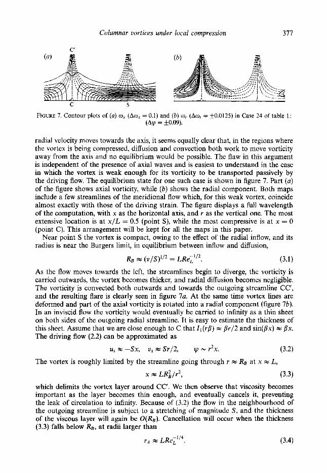
FIGURE 7. Contour plots of (a) ax ( A o x = 0.1) and ( b ) or (Amr = f0.0125) in Case 24 of table 1: (AY, = f0.09).

radial velocity moves towards the axis, it seems equally clear that, in the regions where the vortex is being compressed, diffusion and convection both work to move vorticity away from the axis and no equilibrium would be possible. The flaw in this argument is independent of the presence of axial waves and is easiest to understand in the case in which the vortex is weak enough for its vorticity to be transported passively by the driving flow. The equilibrium state for one such case is shown in figure 7 . Part (a) of the figure shows axial vorticity, while (b) shows the radial component. Both maps include a few streamlines of the meridional flow which, for this weak vortex, coincide almost exactly with those of the driving strain. The figure displays a full wavelength of the computation, with x as the horizontal axis, and r as the vertical one. The most extensive location is at x / L = 0.5 (point S ) , while the most compressive is at x = 0 (point C). This arrangement will be kept for all the maps in this paper.

Near point S the vortex is compact, owing to the effect of the radial inflow, and its radius is near the Burgers limit, in equilibrium between inflow and diffusion,

RB = (v/S)'I2 = LRe-'I2 L . (3 .1)

As the flow moves towards the left, the streamlines begin to diverge, the vorticity is carried outwards, the vortex becomes thicker, and radial diffusion becomes negligible. The vorticity is convected both outwards and towards the outgoing streamline CC', and the resulting flare is clearly seen in figure 7a. At the same time vortex lines are deformed and part of the axial vorticity is rotated into a radial component (figure 7b). In an inviscid flow the vorticity would eventually be carried to infinity as a thin sheet on both sides of the outgoing radial streamline. It is easy to estimate the thickness of this sheet. Assume that we are close enough to C that I l ( r p ) = p r / 2 and sin(px) rn px. The driving flow (2.2) can be approximated as

us w -Sx, us = S r / 2 , y - r x. (3.2)

= L R ; . / ~ ~ , (3.3)

2

The vortex is roughly limited by the streamline going through r = RB at x = L,

which delimits the vortex layer around CC'. We then observe that viscosity becomes important as the layer becomes thin enough, and eventually cancels it, preventing the leak of circulation to infinity. Because of (3.2) the flow in the neighbourhood of the outgoing streamline is subject to a stretching of magnitude S , and the thickness of the viscous layer will again be O(&). Cancellation will occur when the thickness (3.3) falls below RB, at radii larger than

TA W LRe,''4. (3.4)

378 R. Verzicco, J. Jimtnez and P. Orlandi

0.8 i

0 5 10 15 -0.25 0 0.25 0.50 0.75 rl rA X l L

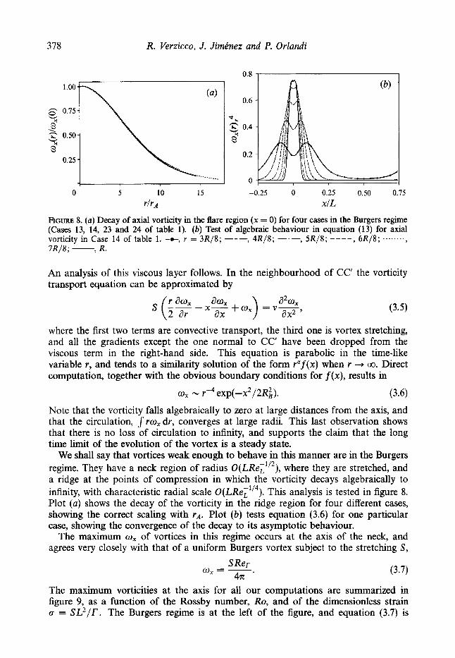
FIGURE 8. (a) Decay of axial vorticity in the flare region (x = 0) for four cases in the Burgers regime (Cases 13, 14, 23 and 24 of table 1). (b) Test of algebraic behaviour in equation (13) for axial vorticity in Case 14 of table 1. -e, r = 3 R / 8 ; ---, 4R/8; -.-, 5 R / 8 ; ----, 6 R / 8 ; ......--, 7R/8; - 7 R.

An analysis of this viscous layer follows. In the neighbourhood of CC’ the vorticity transport equation can be approximated by

where the first two terms are convective transport, the third one is vortex stretching, and all the gradients except the one normal to CC’ have been dropped from the viscous term in the right-hand side. This equation is parabolic in the time-like variable r, and tends to a similarity solution of the form r a f ( x ) when r + 00. Direct computation, together with the obvious boundary conditions for f(x), results in

ox - r-4 exp(-x2/2~i). (3.6)

Note that the vorticity falls algebraically to zero at large distances from the axis, and that the circulation, J rwX dr, converges at large radii. This last observation shows that there is no loss of circulation to infinity, and supports the claim that the long time limit of the evolution of the vortex is a steady state.

We shall say that vortices weak enough to behave in this manner are in the Burgers regime. They have a neck region of radius 0 ( ~ 5 R e , ” ~ ) , where they are stretched, and a ridge at the points of compression in which the vorticity decays algebraically to infinity, with characteristic radial scale 0(LRe,1’4). This analysis is tested in figure 8. Plot (a) shows the decay of the vorticity in the ridge region for four different cases, showing the correct scaling with rA. Plot (b) tests equation (3.6) for one particular case, showing the convergence of the decay to its asymptotic behaviour.

The maximum ox of vortices in this regime occurs at the axis of the neck, and agrees very closely with that of a uniform Burgers vortex subject to the stretching S,

S Rer 4x

0, = -. (3.7)

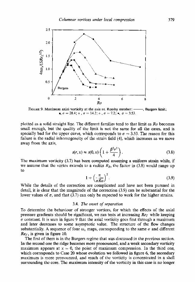
The maximum vorticities at the axis for all our computations are summarized in figure 9, as a function of the Rossby number, Ro, and of the dimensionless strain C-J = SL2/T. The Burgers regime is at the left of the figure, and equation (3.7) is

2.5

2.0

n Q "2 1.5 a: % g 1.0 d

0.5

Columnar vortices under local compression

1

V I I

379

0 2 4 6 8

FIGURE 9. Maximum axial vorticity at the axis us. Rossby number: - , Burgers limit; m, u = 28.4; o , u = 14.2; A , u = 7.2; 0, u = 3.53.

Ro

plotted as a solid straight line. The different families tend to that limit as Ro becomes small enough, but the quality of the limit is not the same for all the cases, and is specially bad for the upper curve, which corresponds to Q = 3.53. The reason for this failure is the radial inhomogeneity of the strain field (4), which increases as we move away from the axis,

S ( I , X ) = s(0,x) (1 + y ) .

The maximum vorticity (3.7) has been computed assuming a uniform strain while, if we assume that the vortex extends to a radius RB, the factor in (3.8) would range up to

While the details of the correction are complicated and have not been pursued in detail, it is clear that the magnitude of the correction (3.9) can be substantial for the lower values of 0, and that (3.7) can only be expected to work for the higher strains.

3.4. The onset of separation To determine the behaviour of stronger vortices, for which the effects of the axial pressure gradients should be significant, we ran tests at increasing Rer while keeping Q constant. It is seen in figure 9 that the axial vorticity goes first through a maximum and later decreases to some asymptotic value. The structure of the flow changes substantially. A sequence of four ox maps, corresponding to the same 0 and different Rer, is given in figure 10.

The first of them is in the Burgers regime that was discussed in the previous section. In the second one the ridge becomes more pronounced, and a weak secondary vorticity maximum appears at x = 0, the point of maximum compression. In the third one, which corresponds to Case 20 whose evolution we followed in figure 6, the secondary maximum is more pronounced, and much of the vorticity is concentrated in a shell surrounding the core. The maximum intensity of the vorticity in this case is no longer

380 R. Verzicco, J. Jirndnez and P. Orlandi

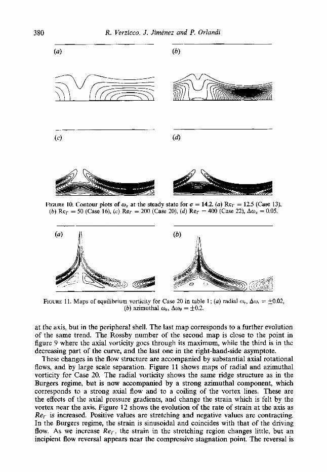
FIGURE 10. Contour plots of ox at the steady state for c = 14.2. (a) Rer = 12.5 (Case 13), ( b ) Rer = 50 (Case 16), ( c ) Rer = 200 (Case 20), ( d ) Rer = 400 (Case 22), Aw, = 0.05.

FIGURE 11. Maps of equilibrium vorticity for Case 20 in table 1 ; (a) radial wr, Aur = $0.02, (b) azimuthal 08, Awe = k0.2.

at the axis, but in the peripheral shell. The last map corresponds to a further evolution of the same trend. The Rossby number of the second map is close to the point in figure 9 where the axial vorticity goes through its maximum, while the third is in the decreasing part of the curve, and the last one in the right-hand-side asymptote.

These changes in the flow structure are accompanied by substantial axial rotational flows, and by large scale separation. Figure 11 shows maps of radial and azimuthal vorticity for Case 20. The radial vorticity shows the same ridge structure as in the Burgers regime, but is now accompanied by a strong azimuthal component, which corresponds to a strong axial flow and to a coiling of the vortex lines. These are the effects of the axial pressure gradients, and change the strain which is felt by the vortex near the axis. Figure 12 shows the evolution of the rate of strain at the axis as Re= is increased. Positive values are stretching and negative values are contracting. In the Burgers regime, the strain is sinusoidal and coincides with that of the driving flow. As we increase R e r , the strain in the stretching region changes little, but an incipient flow reversal appears near the compressive stagnation point. The reversal is


-0.2 tL , , , -"!0.25 0 0.25 0.50 0.15

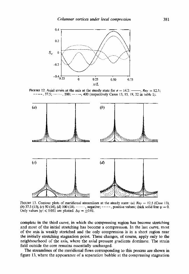
x/L FIGURE 12. Axial strain at the axis at the steady state for cr = 14.2: - , Rer = 12.5;

---- > , 37.5. .....-.. 2 ) 100- ---, 400 (respectively Cases 13, 15, 18, 22 in table 1).

FIGURE 13. Contour plots of meridional streamlines at the steady state: (a) Rer = 12.5 (Case 13), (b) 37.5 (15), (c) 50 (16), (d ) 100 (18). --.---.-,negative; ---- , positive values; thick solid line I,U = 0. Only values IwI < 0.051 are plotted. Ay = 90.01.

complete in the third curve, in which the compressing region has become stretching and most of the initial stretching has become a compression. In the last curve, most of the axis is weakly stretched and the only compression is in a short region near the initially stretching stagnation point. These changes, of course, apply only to the neighbourhood of the axis, where the axial pressure gradients dominate. The strain field outside the core remains essentially unchanged.

The streamlines of the meridional flows corresponding to this process are shown in figure 13, where the appearance of a separation bubble at the compressing stagnation

382 R. Verzicco, J . Jirntnez and P. Orlandi

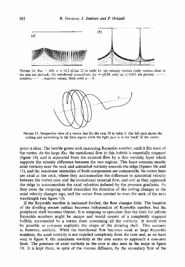
FIGURE 14. Rer = 400, 0 = 14.2 (Case 22 in table 1): (a) velocity vectors (only vectors close to the axis are plotted); ( b ) meridional streamlines, Av = hO.01, only Iy( < 0.051 are plotted. ----, positive; ....----, negative values; thick solid y = 0.

FIGURE 15. Perspective view of a vortex line for the case 20 in table 1. The left part shows the coiling and unwinding in the flare region while the right part is in the ‘neck’ of the vortex.

point is clear. The bubble grows with increasing Reynolds number, until it fills most of the vortex. At the large Rer the meridional flow in this bubble is essentially stagnant (figure 14), and is separated from the external flow by a thin vorticity layer which supports the velocity difference between the two regions. This layer contains mostly axial vorticity near the neck and azimuthal vorticity towards the ridge (figures 1Oc and ll), and the maximum intensities of both components are comparable. Its vortex lines are axial at the neck, where they accommodate the difference in azimuthal velocity between the vortex core and the irrotational external flow, and coil as they approach the ridge to accommodate the axial velocities induced by the pressure gradients. As they cross the outgoing radial streamline the direction of the coiling changes as the axial velocity changes sign, and the vortex lines unwind to meet the neck of the next wavelength (see figure 15).

If the Reynolds number is increased further, the flow changes little. The location of the dividing stream surface becomes independent of Reynolds number, but the peripheral shell becomes thinner. It is tempting to speculate that the limit for infinite Reynolds numbers might be unique and would consist of a completely stagnant bubble, surrounded by a vortex sheet containing all the vorticity. It would then be possible to compute explicitly the shape of the dividing shell. This scenario is, however, unlikely. While the meridional flow becomes weak at large Reynolds numbers, the axial vorticity is not expelled completely from the core and, as we have seen in figure 9, the maximum vorticity at the axis seems to approach a non-zero limit. The presence of axial vorticity in the core is also seen in the maps in figure 10. It is kept there, in spite of the viscous diffusion, by the secondary flow of the


1.0-

O X

0.5 -

(a)

.....

separation bubble, and it should be observed that there is a possible limit in which a vortex with vanishing viscosity can be kept concentrated by a secondary flow of vanishing intensity.

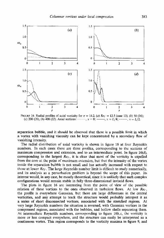
The radial distribution of axial vorticity is shown in figure 16 at four Reynolds numbers. In each cases there are three profiles, corresponding to the sections of maximum compression and extension, and to an intermediate point. In figure 16(d), corresponding to the largest Rer, it is clear that most of the vorticity is expelled from the core at the point of maximum extension, but that the intensity of the vortex inside the separation bubble is not small and has actually increased with respect to those at lower Rer. The large Reynolds number limit is difficult to study numerically, and its analysis as a perturbation problem is beyond the scope of this paper. Its interest would, in any case, be mostly theoretical, since it is unlikely that such complex configurations would remain stable in fully three-dimensional inviscid flows.

The plots in figure 16 are interesting from the point of view of the possible relation of these vortices to the ones observed in turbulent flows. At low Rer, the profile is everywhere Gaussian, but there are large differences in the central vorticities, and any attempt to track the structure would probably interpret it as a series of short disconnected vortices, associated with the stretched regions. At very large Reynolds numbers the situation is reversed, with Gaussian vortices in the compressed regions, associated with the bubbles, and hollow shells separating them. At intermediate Reynolds numbers, corresponding to figure 16b, c, the vorticity is more or less compact everywhere, and the structure can easily be interpreted as a continuous vortex. This region corresponds to the vorticity maxima in figure 9, and

384 R. Verzicco, J . Jimdnez and P. Orlandi

it is the most likely candidate for the identification of the long vortices observed in turbulent flows.

The coiling of the vortex lines, and the presence of a stagnant bubble has been reported often for the related phenomenon of vortex breakdown (e.g. Leibovich 1978; Lhpez 1990), and the importance of azimuthal vorticity has been stressed both for the generation of axial waves (Melander & Hussain 1994) and for the initiation of vortex breakdown (Brown & L6pez 1990).

3.5. The criterion for separation

The Rossby number used in figure 9 to display the results of the numerical experiments was introduced in equation (2.4) as the ratio of azimuthal to axial velocities for a vortex with a radius of the order of the Burgers length RB. Criteria based on swirl numbers of this type have been proposed often as onset criteria for vortex breakdown (Leibovich 1978; Keller, Egli & Exley 1985, and references in the introduction of Brown & L6pez 1990). Since our separation occurs on vortices near the Burgers’ limit, it was hoped that a swirl number based on that radius would be useful as a criterion to predict its onset. It is clear from figure 9 that this is not so, and that there is no collapse among the different curves when plotted in terms of Ro. In retrospect this is not surprising, since our vortices are not cylindrical and there is a whole range of radii and axial velocities. Swirl number criteria tend to be based on linearized analyses of uniform vortices, and it was already noted in Brown & L6pez (1990) that they did not work for their confined breakdown.

On the other hand, since we have a reasonably clear idea of the structure of our flow, and of the phenomena which accompany separation, it is fairly easy to construct a qualitative criterion for its onset. We know that the first symptom is the appearance of a small separation bubble at the axis at x = 0, which corresponds to a reversal of the axial strain at that point from compressive to extensive. This has to be due to the effect of the axial pressure gradients generated by the centrifugal forces in the vortex, to which the analysis in 53.3 should still apply.

Consider a vortex shape defined by the streamline in equation (3.3), which can be rewritten near x = 0 as

R NN RB(x /L) - ’ / ’ . (3.10) The characteristic azimuthal velocity in such a vortex is ue = T / R and the pressure drop across the core is

(3.11)

Since this pressure gradient is responsible for the axial flow, we obtain from Bernouilli’s theorem along the axis

(3.12)

This induced velocity moves along the axis away from the origin, and tends to counteract the velocity of the driving flow, us w -Sx . Since up behaves like a lower power of x , this simple theory predicts that the induced velocity always wins close to the origin, and that there is always a separation bubble. By equating the magnitude of both velocities, the size of this bubble can be shown to be proportional to L Ro’.

It is easy to see that this estimate is wrong for small Ro, because (3.11) is a boundary layer approximation which assumes a slender vortex in which longitudinal gradients are negligible with respect to radial ones. This is not true near x = 0, where

5

1


Burgers

I I I I

0 5 10 15 20 25

Rer lReLIi3

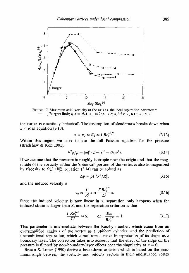
FIGURE 17. Maximum axial vorticity at the axis us. the local separation parameter: , Burgers limit; m, 0 = 28.4; o , 14.2; A , 7.2; 0, 3.53; x , 6.12; + , 21.2.

the vortex is essentially 'spherical'. The assumption of slenderness breaks down when x < R in equation (3.10),

x < xo w & w LRei'/3. (3.13) Within this region we have to use the full Poisson equation for the pressure (Bradshaw & Koh 1981),

v2p/p = 1012/2 - )Sl2 = O ( 0 2 ) . (3.14)

If we assume that the pressure is roughly isotropic near the origin and that the magnitude of the vorticity within the 'spherical' portion of the vortex is also homogenized by viscosity to O(r/g), equation (3.14) can be solved as

and the induced velocity is

(3.16)

Since the induced velocity is now linear in x , separation only happens when the induced strain is larger than S , and the separation criterion is that

(3.17)

This parameter is intermediate between the Rossby number, which came from an oversimplified analysis of the vortex as a uniform cylinder, and the prediction of unconditional separation, which came from a naive interpretation of its shape as a boundary layer. The correction takes into account that the effect of the ridge on the pressure is filtered by non-boundary-layer effects near the singularity at x = 0.

Brown & L6pez (1990) derive a breakdown criterion which is based on the maximum angle between the vorticity and velocity vectors in their undisturbed vortex

386 R. Verzicco, J . Jimknez and P. Orlandi

cores. That criterion is inapplicable here, because our pressure gradient is part of the boundary conditions, and there is no ‘undisturbed’ state. In fact, it is easy to show that the maximum angle between the vorticity and the velocity is always n/2 in our case.

The data in figure 9 are replotted in figure 17, in terms of the new parameter. The collapse is now much better, specially for the high-o cases in which the effect of radial inhomogeneity of the strain (equation (3.9)) is absent. In particular the location of the maximum vorticity, which signals the onset of separation, is now almost the same for all values of 0, while previously it varied by over a factor of two in Ro. Also, the two curves corresponding to the highest 0 coincide almost exactly over the whole range of Reynolds numbers.

4. Conclusions We have shown that steady-state vortices can form under the effect of inhomo-

geneous straining, even in the case in which the axial mean value of the applied strain is zero. Even in that case, in which it can be said that the vortex is not being stretched at all, the mean radius of the vortex is close to the Burgers radius corresponding to the magnitude of the strain fluctuation. This is specially so in a narrow range of vortex circulations, in which Rer w Weaker vortices tend to break into disconnected pieces, associated with the locations at which the stretching is maximum, and separated by gaps where the vortex is compressed. Stronger vortices break down under the effect of the induced axial pressure gradients.

The structure of the flow has been studied in detail, and a theoretical analysis has been presented for the weak vortex limit and the onset of separation.

The investigation was motivated by the observation of long strong vortices in turbulence, with diameters which are of the order of the Kolmogorov scale q, but with lengths which are much longer (Jimknez et al. 1993). It has been shown from direct numerical simulations that the axial strains in these vortices are of the order of the root-mean-square vorticity m’, whose Burgers radius is q (Jimknez & Wray 1994a), and that the correlation scale for this strain is again q (Jimknez & Wray 1994b). The results of the present work are fully consistent with the first part of those observations, since they show that it is the fluctuating part of the strain, not its average, which determines the radius. They also help to explain why the vortex can be much longer than the correlation length of the driving strain, since we have shown that they can be essentially infinite for periodic strains.

The second goal of the investigation, to explain the empirical correlation (1.1) between the intensity of the vortices and the microscale Reynolds number of the turbulent flow, is less successful. It will be remembered that the experimental relation was Rer - Re!, with a in the range 0.3-0.5. Since the criterion for the onset of separation, and for the existence of vortices that would be identified as such, is given by equation (3.17), it is tempting to associate L to the Taylor microscale, and to use the present relation as a justification for the experimental one. We cannot, however, find any convincing reason for that association, and it seems to contradict the experimental measurements of the axial correlation length of the strain as q. The axial Reynolds number corresponding to a strain m’ with wavelength q is ReL - 1.

Perhaps the most successful conclusion of the present work, as it relates to turbulence, is the explanation of why the velocity components of a turbulent flow are free of intermittency effects (Anselmet et al. 1984). From the moment that strong columnar vortices were discovered in turbulence, this observation became a problem,


since a strong strained vortex creates large azimuthal velocities. It was noted in Jimenez et al. [ 1993) that the empirical relation for the growth of Re= as a function of Red just avoided this dficulty. The circulation of the strongest vortices was just such that their azimuthal velocities were independent of Red, and were always of the same order as the root-mean-square velocity of the flow u’. The reason for that was not clear at the time, and it was hypothesized that it was due to the formation of the vortices from the roll-up of vortex sheets, which do not amplify velocity as they are strained. It was never clear, however, why vortex sheets did not roll up until they had reached their final intensities, or why the vortices were not stretched after they formed.

The present paper offers a different explanation. It turns out that the stretching of a circular vortex cannot amplify velocity beyond the total velocity difference applied between its end points. Consider an ‘optimum’ vortex such that equation (3.17) is satisfied. Its minimum radius is still O(RB), and its maximum azimuthal velocity is ug = r / R B . The maximum axial velocity difference applied to it is AU m SL, and the ratio of the two is

As a consequence, the mechanism of the turbulent cascade has no way of amplifying velocities, even if it amplifies velocity gradients through vortex stretching, and velocity intermittency does not develop. Note that this limiting mechanism would have some influence in the formulation of models for the intermittency of the gradients, since most of them assume a more or less unconstrained amplification of vorticity, while the present mechanism, imposed by the nonlinear effect of axial pressure gradients, represents a global limit on how far gradients can be amplified.

The research was partially supported by the Human Capital and Mobility program of the EC under contract CHRXCT920001, and by a grant from “Minister0 dell’ Universita e della Ricerca Scientifica e Tecnologica”, MURST MPI 60%. This work was partially motivated by a discussion on velocity intermittency with E. Hopfinger.

REFERENCES

ANSELMET, E, GAGNE, Y., HOPFINGER, E. J. & ANTONIA, R. A. 1984 High order velocity structure

BERAN, P. S. & CULICK, F. E. C. 1992 The role of non-uniqueness in the development of vortex

BENJAMIN, T. B. 1962 Theory of vortex breakdown phenomenon. J. Fluid Mech. 14, 593-629. BRADSHAW, P. & KOH, Y. M. 1981 A note on Poisson’s equation for pressure in a turbulent flow.

BROWN, G. L. & L ~ P E Z , J. M. 1990 Axisymmetric vortex breakdown. Part 2. Physical mechanisms.

CAFLISCH, R. E., LI, X. & SHELLEY, M. J. 1993 The collapse of an axi-symmetric, swirling vortex

HOSOKAWA, I. & YAMAMOTO, K. 1990 Intermittency of dissipation in directly simulated fully

JIM~NEZ, J. & WRAY, A. A. 1994a Columnar vortices in isotropic turbulence. Meccanica 29,453-464. JIM~NEZ, J. & WRAY, A. A. 1994b The dynamics of intense vorticity in isotropic turbulence. CTR

JIM~NEZ, J. WRAY, A. A., SAFFMAN, P. G. & ROGALLO, R. S. 1993 The structure of intense vorticity

KELVIN, LORD 1880 Vibrations of a columnar vortex. Phil. Mag. 10, 155-168.

functions in turbulent shear flows. J. Fluid Mech. 140, 63-89.

breakdown in tubes. J. Fluid Mech. 242, 491-527.

Phys. Fluids 24, 777.

J. Fluid Mech. 221, 553-576.

sheet. Nonlinearity 4, 843-867.

developed turbulence. J. Phys. SOC. Japan 59, 401-404.

Annual Res. Briefs 1994.

in isotropic turbulence. J. Fluid Mech. 255, 65-90.

388 R. Verzicco, J . Jimtnez and P. Orlandi

KELLER, J. J, EGLI, W. & EXLEY, J. 1985 Force- and loss-free transitions between flow states. 2.

KERR, R. M. 1985 Higher order derivative correlation and the alignment of small-scale structure in

LEIBOVICH, S. 1978 Structure of vortex breakdown. Ann. Reo. Fluid Mech. 10, 221-246. LEONARD, A. 1994 Nonlocal theory of area-varying waves on axisymmetric vortex tubes. Phys.

LOPEZ, J. M. 1990 Axisymmetric vortex breakdown. Part 1. Confined swirling flows. J. Fluid Mech.

LUNDGREN, T. S. & ASHURST, W. T. 1989 Area-varying waves on curved vortex tubes with application

MELANDER, M. V. & HUSSAIN, F. 1994 Core dynamics on a vortex column. Fluid Dyn. Res. 13,

MOORE, D. W. & SAFFMAN, P. G. 1972 The motion of a vortex filament with axial flow. Phil. Trans.

ROGALLO, R. S . 1981 Numerical experiments in homogeneous turbulence. NASA 734-81315. RUETSCH, G. R. & MAXEY, M. R. 1991 Small scales features of vorticity and passive scalar fields in

SHE, Z.-S. , JACKSON, E. & ORSZAG, S. A. 1990 Intermittent vortex structures in homogeneous

SIGGIA, E. D. 1981 Numerical study of small scale intermittency in three-dimensional turbulence. J.

VERZICCO, R. & ORLANDI, P. 1993 A finite-difference scheme for three-dimensional incompressible

VERZICCO, R. & ORLANDI, P. 1994 Normal and oblique collisions of a vortex ring with a wall.

VINCENT, A. & MENEGUZZI, M. 1991 The spatial structure and statistical properties of homogeneous

Angew. Math. Phys. 36,854-889.

isotropic numerical turbulence. J. Fluid Mech. 153, 31-58.

Fluids 6, 765-777.

221, 533-552.

to vortex breakdown. J. Fluid Mech. 200, 283-307.

1-37.

R. SOC. b n d . A 212,47429.

homogeneous isotropic turbulence. Phys. Fluids A 3, 1587-1597.

isotropic turbulence. Nature 344, 226-228.

Fluid Mech. 107, 375-406.

flows in cylindrical coordinates. J . Comput. Phys. (submitted).

Meccanica 29, 383-391.

turbulence. J. Fluid Mech. 225, 1-25.

On steady columnar vortices under local compression · On steady columnar vortices under local...

Documents

Transcript of On steady columnar vortices under local compression · On steady columnar vortices under local...