On Self-Timed Circuits in Real-Time Systems

Hindawi Publishing CorporationInternational Journal of Reconfigurable ComputingVolume 2011, Article ID 972375, 16 pagesdoi:10.1155/2011/972375

Research Article

On Self-Timed Circuits in Real-Time Systems

Markus Ferringer

Department of Computer Engineering, Embedded Computing Systems Group, Vienna University of Technology,Treitlstraße 3, 1040 Vienna, Austria

Correspondence should be addressed to Markus Ferringer, [email protected]

Received 6 August 2010; Accepted 8 January 2011

Academic Editor: Michael Hubner

Copyright © 2011 Markus Ferringer. This is an open access article distributed under the Creative Commons Attribution License,which permits unrestricted use, distribution, and reproduction in any medium, provided the original work is properly cited.

While asynchronous logic has many potential advantages compared to traditional synchronous designs, one of the majordrawbacks is its unpredictability with respect to temporal behavior. Having no high-precision oscillator, a self-timed circuit’sexecution speed is heavily dependent on temperature and supply voltage. Small fluctuations of these parameters already resultin noticeable changes of the design’s throughput and performance. Without further provisions this jitter makes the use ofasynchronous logic hardly feasible for real-time applications. We investigate the temporal characteristics of self-timed circuitsregarding their usage in real-time systems, especially the Time-Triggered Protocol. We propose a simple timing model and elaboratea self-adapting circuit which shall derive a suitable notion of time for both bit transmission and protocol execution. We furtherintroduce and analyze our jitter compensation concept, which is a threefold mechanism to keep the asynchronous circuit’s notionof time tightly synchronized to the remaining communication participants. To demonstrate the robustness of our solution, weperform different tests and investigate their impact on jitter and frequency stability.

1. Introduction

Asynchronous circuits elegantly overcome some of thelimiting issues of their synchronous counterparts. The often-cited potential advantages of asynchronous designs are—among others—reduced power consumption and inherentrobustness against changing operating conditions [1, 2].Recent silicon technology additionally suffers from highparameter variations and high susceptibility to transientfaults [3]. Asynchronous (delay insensitive) design offers asolution due to its inherent robustness. A substantial part ofthis robustness originates in the ability to adapt the speedof operation to the actual propagation delays of the under-lying hardware structures, due to the feedback formed bycompletion detection and handshaking. While asynchronouscircuits’ adaptive speed is hence a desirable feature withrespect to robustness, it becomes a problem in real-timeapplications that are based on a stable clock and a fixed(worst-case) execution time. Therefore, asynchronous logicis commonly considered inappropriate for such real-timeapplications, which excludes its use in an important shareof fault-tolerant applications that would highly benefit fromits robustness. Consequently, it is reasonable to take a closer

look at the actual stability and predictability of asynchronouslogic’s temporal behavior. After all, synchronous designsoperate on the same technology, but hide their imperfectionswith respect to timing behind a strictly time-driven controlflow that is based on worst-case timing analysis. Thismasking provides a convenient, stable abstraction for higherlayers. In contrast, asynchronous designs simply allow thevariations to happen and propagate them to higher layers.Therefore, the interesting questions are as follows: whichcharacter and magnitude do these temporal variations have?Can these variations be tolerated or compensated to allow theusage of self-timed circuits in real-time applications?

In our research project ARTS (Asynchronous Logic inReal-Time Systems) we are aiming to find answers to thesequestions. The project goal is to design an asynchronousTTP (Time-Triggered Protocol) controller prototype whichis able to reliably communicate with a set of synchronousequivalents even under changing operating conditions. TTPwas chosen for this reference implementation because itcan be considered as an outstanding example for hard real-time applications. In this paper we present results basedon our previous and current work. We will investigate

2 International Journal of Reconfigurable Computing

the capabilities of self-timed designs to adapt themselvesto changing operating conditions. With respect to ourenvisioned asynchronous TTP controller we will define atiming model, and also study the characteristics of jitter(and the associated frequency instabilities of the circuit’sexecution speed) as well as the corresponding compensationmechanisms. We implement and investigate a fully func-tional transceiver unit, as required for the TTP controller, todemonstrate the capabilities of the proposed solution withrespect to TTP’s stringent requirements.

The work is structured as follows. In Section 2 wegive some important background information on TTP, theresearch project ARTS, and the used asynchronous designstyle. Section 3 discusses related work and the basic jitterterminology. Afterwards, Section 4 discusses temporal char-acteristics of QDI circuits and presents some case studies.The main requirements, properties, and implementationdetails of the asynchronous time reference generation unitare presented in Section 5, right before experimental resultsare shown in Section 6. The paper concludes in Section 7with a short summary and an outlook to future work.

2. Background

2.1. Time-Triggered Protocol. The Time-Triggered Protocol(TTP) has been developed for the demanding requirementsof distributed (hard) real-time systems. It provides severalsophisticated means to incorporate fault-tolerance and at thesame time keep the communication overhead low. TTP usesextensive knowledge of the distributed system to implementits services in a very efficient and flexible way. Real-timesystems in general and TTP in particular are described indetail in [4, 5].

A TTP system generally consists of a set of Fail-SilentUnits (FSUs), all of which have access to two replicatedbroadcast communication channels. Usually two FSUs aregrouped together to form a Fault-Tolerant Unit (FTU),as illustrated in Figure 1(a). In order to access the com-munication channel, a TDMA (Time Division MultipleAccess) scheme is implemented. As illustrated in Figure 1(b),communication is organized in periodic TDMA rounds,which are further subdivided into various sending slots. Eachnode has statically assigned sending slots, thus the entireschedule (called Message Descriptor List, MEDL) is knownat design-time already. Since each node a priori knows whenother nodes are expected to access the bus, message collisionavoidance, membership service, clock synchronization, andfault detection can be handled without considerable com-munication overhead. Explicit Bus Guardian (BG) units areused to limit bus access to the node’s respective time slots,thereby solving the babbling idiot problem. Global time iscalculated by a fault-tolerant, distributed algorithm whichanalyzes the deviations of the expected and actual arrivaltimes of messages and derives a correction term at each node.

The Time-Triggered Protocol provides very powerfulmeans for developing demanding real-time applications. Thehighly deterministic and static nature makes it seeminglyunsuited for an implementation based on asynchronous

FTU

FSU

TTP

BGBG

FTU

FSU

TTP

BGBG

FTU

FSU

TTP

BGBG

FSU

TTP

BGBG

FSU

TTP

BGBG

FSU

TTP

BGBG

(a)

n1 n2 n · · · n1 n2 n · · · · · ·

TDMA round Nodes’ slots

Cluster cycle

(b)

Figure 1: TTP system structure (a) and TDMA communicationscheme (b).

logic, as a precise notion of time (which is usually providedby a crystal oscillator in synchronous systems) is missing.Hence, these properties also make TTP an interesting andchallenging topic for our exploration of predictability of self-timed logic.

2.2. ARTS Project. The aim of the ARTS (AsynchronousLogic in Real-Time Systems) research project is to investigatethe temporal predictability and stability of asynchronous(QDI, quasi delay insensitive) hardware designs. Morespecifically, we want to compile models for the timinguncertainties of hardware execution times and extend theseto make quantitative statements on the timing behaviorof self-timed circuits. Our hope is that the theoreticaland experimental analyses will also provide indications forimproving the temporal stability of self-timed circuits.

The central concern for the project is the predictabilityof asynchronous logic with respect to its temporal prop-erties. We therefore investigate jitter sources (e.g., data-dependencies, voltage fluctuations, temperature drift) andclassify their impact on the execution time. Using an ade-quate model allows us to identify critical parts in the circuitand implement measures for compensation. Another issueconcerns timeliness itself, as without a reference clock we donot have an absolute notion of time. Instead, we will use thestrict periodicity of TTP to continuously resynchronize to thesystem and derive a time-base for message transfer.

The tangible project result shall be an asynchronousimplementation of a TTP controller operating in an ensem-ble of conventional, synchronous controllers as illustrated inFigure 2(a). It is evident from the explanation in Section 2.1that TTP’s static bus access schedule as well as its clocksynchronization and data transmission protocol rely onthe stability of the constituent nodes’ local clock sources.Therefore it seems quite daring to implement the controllerlogic in an asynchronous design style. However, movingsuch a deeply synchronous application to an asynchronousimplementation is an interesting and informative challengeof its own, and—if we are successful—a very convincing

International Journal of Reconfigurable Computing 3

Self-timed

TTP

TTP

TTP

TTP

CCC

C

TT

P-bu

s

(a)

Communication network interface(CNI)

Host CPU

Dual ported RAMMEDL

Ref-time

TTP core

TTP-bus

Syn

chro

nou

sA

syn

chro

nou

s

TxD RxD

(b)

Figure 2: ARTS system setup (a) and TTP-node block diagram (b).

case study for demonstrating the temporal predictability ofasynchronous logic. In this context we need to solve twofundamental problems, whereby it is mandatory to derivequantitative boundaries for the attained properties in bothcases.

(1) We have to make our design operate stable enoughto meet TTP’s stringent requirements on executiontimes and jitter. Conceptually this issue has to dowith the fact that control flow in self-timed circuitsis flexible and not strictly time-driven, as in thesynchronous paradigm.

(2) We have to provide a stable local time reference forbit timing and bus access. This issue originates fromthe fact that in synchronous systems the clock sourcescan also be used as time reference—which is missingin a self-timed approach.

Figure 2(b) shows the internal structure of the envisionedasynchronous TTP node. It is very similar to the existing TTPcommunication chip from TTTech Computertechnik AG[6], our project partner. The interface to the controlling host-CPU (CNI, Communication Network Interface) will remainsynchronous, thus existing soft and hardwaresolutions forTTP can be used without modifications. However, the“central” parts (bus access, receiver-unit, transmitter-unit,macrotick generation, TTP-services, etc.) of the controllerwill be replaced by asynchronous implementations. Similarto the existing FPGA-based controller, a dual-ported RAMseparates the CNI from the TTP-core, thereby formingnot only a temporal firewall [5], but also splitting thesynchronous from the asynchronous parts. (Both host-CPU and TTP controller share a global time-base, thusconcurrent access to the dual-ported RAM can be controlledto avoid collisions.) It should be noted that the asynchronouscontroller implementation is intended solely as an academiccase study and not as a prototype for an industrial design.However, a successful project outcome might considerablyincrease acceptance and even open new fields of applicationsfor asynchronous designs.

The main challenge relies in the method of resynchro-nization, as the controller will use the data stream provided

by the other communication participants to dynamicallyadapt its internal time reference. The chosen solution is touse a free-running, self-timed counter for measuring theduration of external events of known length (i.e., singlebits in the communication stream). The so gained referencemeasurement can in turn be used to generate ticks withthe period of the observed event. This local time-baseshould enable the asynchronous node to derive a sufficientlyaccurate time reference for both low-level communication(bit-timing, data transfer) as well as high-level services (e.g.,macrotick generation). The disturbing impact of environ-mental fluctuations is automatically compensated over time,because periodic resynchronization will lead to differentreference measurements, depending on the current speed ofthe counter circuit.

2.3. Asynchronous Design Style. Our focus is on QDI(quasi delay insensitive) circuits, as they exhibit morepronounced “asynchronous” properties than bounded delaycircuits. More specifically, we use the level-encoded dual-rail approach (LEDR [7, 8], used in Phased Logic [9], e.g.),which represents a logic signal on two physical wires. Weprefer the more complex 2-phase implementation over thepopular 4-phase protocol [2, 10], as it is more elegant andwe have already gained some practical experience with it.LEDR periodically alternates between two disjoint code setsfor representing logic “HI” and “LO” (two phases ϕ0 andϕ1, see Figure 3(a)), thus avoiding the need to insert NULLtokens as spacers between subsequent data items.

In this approach, completion detection comes downto a check whether the phases of all associated signalshave changed and match. As usual, handshaking betweenregister/pipeline stages is performed by virtue of a capturedone signal. Figure 3(b) shows an exemplary LEDR circuitwith two sequential registers (reg0→ 2) and a feedback loop(reg0→ 1→ 0). Direct feedback (i.e., without a shadow registerlike reg1) is not possible, as race conditions and deadlocksmay occur when a register issues its own acknowledges andrequests. Also notice the phase inverter in the feedback path.

If external single-rail inputs are to be fed into LEDRcircuits, special “interface gates” [9] must properly align


I(0, 0)ϕ0

L(0, 1)ϕ1

H(1, 0)ϕ1

h(1, 1)ϕ0

“HI”

“LO”

(a)cD

one

Data

reg 0

reg 1

reg 2

ϕ

C

(b)

Figure 3: LEDR coding (a) and exemplary LEDR circuit structure(b).

(“synchronize”) these to the LEDR operation cycles. Con-crete implementations and variations of such interface gatesare described in [11].

The two-rail coding as well as the adaptive timingmake LEDR circuits very robust against faults and changingoperating conditions, unfortunately at the cost of increasedarea consumption and reduced performance. In principle,LEDR circuits belong to the class of QDI circuits, andtypically the mandatory delay constraints are hidden insidethe basic building blocks, while the interfaces between thesemodules are considered delay insensitive (i.e., unconstrainedwith respect to their timing delays).

2.4. Design Flow. For efficiently implementing complexasynchronous circuits it is of upmost importance that thereexists a sophisticated software tool support. This is the mainreason why the special area of automated synchronous-to-asynchronous converters gains more and more interest.This procedure, which is also called desynchronization, hasthe major advantage that designers need not care aboutthe fallacies and pitfalls of asynchronous design directly.The systems can be described in a synchronous fashion,and an (optimally fully) automated tool chain converts itaccordingly. A good overview to existing design flows usingautomated circuit conversion has recently been presented in[12]. The approach taken at our department [13] is also aform of desynchronization, and is explained in more detailin the next few paragraphs.

The general idea behind automated circuit conversion isto use a suitable circuit representation (one which designersare familiar with), and let a software tool convert the circuitinto an asynchronous representation. In the process, the toolneeds to identify concurrency, as well as temporal (temporalmeans the order of events; the exact timing is of coursedifferent because of the different design style) and causaldependencies, and must of course guarantee functional andtemporal equivalence between the input and output circuits.Using an arbitrary synthesis tool, the synchronous designis compiled into a gate-level netlist consisting only of D-flip-flops and the supported combinational gates. Based onthis netlist our tool replaces the all sequential componentswith asynchronous registers, and all logic gates with their(dual-rail) asynchronous counterparts. After analyzing alldependencies, the tool automatically derives an initial token

configuration, inserts shadow registers where necessary andfinally produces the asynchronous netlist. This file can nowbe used for simulation or compilation (technology mapping,placement and routing, . . .) with any suitable software. Thepresented approach has the advantage that it is almost totallyautomated. In addition, designers are not restricted to aspecial asynchronous design style. Our tool is currentlycapable of generating LEDR as well as NCL (Null ConventionLogic) circuits.

3. State of the Art

3.1. Related Work. As already mentioned, the focus of thispaper will be on how to attain a stable time reference in thecontext of self-timed logic. From an abstract point of viewthis problem results from our attempt to insert a self-timedTTP node into an ensemble of otherwise fully synchronousnodes. For the purpose of our project, however, this is animportant part of the deal, and situations like this may beencountered in practice as well. Let us first review somecommon options for building a time reference [14].

(1) Crystal Oscillators. This approach exploits mechan-ical vibrations paired with the piezoelectric effect,which attains highest precision at high frequencies.One of the severe drawbacks of crystal oscillators istheir incompatibility with standard process technol-ogy. They need to be attached externally, which isarea consuming, costly, and unreliable (as solderingcontacts may break in harsh environments). Anotherdrawback is the relatively long startup time of crystaloscillators (in the range of about ten milliseconds).Furthermore, susceptibility to mechanical vibrations,humidity and shock are considerably higher com-pared to alternative solutions.

(2) RC Oscillators [15]. Here the time constant associatedwith charging a capacitance over a resistor is usedas a time reference. While resistors and capacitorsare very cheap components and can be integrated onsilicon, they suffer from high fabrication variationsas well as relatively large temperature and supplyvoltage dependencies. RC oscillators provide a goodalternative to external crystal resonators, as long ashigh frequency and high-precision are not majorconcerns.

(3) Integrated Silicon (Ring-)Oscillators. In this approachthe oscillations produced by a negative digital feed-back loop, usually a ring spanning an odd number ofinverters, are exploited [16]. The implementation isfully compatible with the CMOS fabrication process,but the produced frequency is determined by thedelay path through the closed loop and hence heavilydependent on fabrication variations, supply voltage,and temperature. Different circuit structures areconceivable, from a simple chain of inverters to morecomplex solutions, as for example a free running self-timed circuit based on micropipelines [17].


(4) Distributed Clock Generation [18]. For the use inembedded systems, distributed algorithms can beimplemented to generate clock signals in a fault-tolerant distributed way. Each node can have itsown clock source (i.e., an instance of the distributedalgorithm) that remains in synchrony with the otherswithin some known precision bounds. This approachcan be viewed as a complex distributed silicon ringoscillator, inheriting the properties of the methodabove, but being more complex and robust due to thedesired fault tolerance.

Obviously, the most straightforward solution in oursetting is the use of the self-timed circuit’s natural pro-cessing cycles as a time reference. Being able to exploit theoscillations of self-timed circuits as a replacement for thecrystal oscillator directly meets our project goals. We donot consider solution (4) as it is overly complex for ourapplication.

Another important alternative for generating precisetime references are self-timed oscillator rings, which seemto be perfectly suited for the chosen asynchronous designmethodology. In contrast to (3) they are based on Suther-land’s micropipelines instead of a simple chain of cascadedinverters. A lot of research has been conducted on self-timedoscillator rings. For example, in [19] a methodology for usingself-timed circuitry for global clocking has been proposed.The same authors also used basic asynchronous FIFO stagesto generate multiple phase-shifted clock signals for high-precision timing in [17]. Furthermore, it has been found thatevent spacing in self-timed oscillator rings can be controlled[16, 20]. The Charlie- and the drafting-effects have therebybeen identified as major forces controlling event spacing inself-timed rings [17, 21].

3.2. Jitter. In synchronous systems we have the abstractionof an equally spaced time grid to which all transitionsare aligned, and all deviations from this ideal behavior arecommonly subsumed under the term jitter. Often jitter isassociated with a synchronous clock source like a crystaloscillator, where it is obviously an undesired effect. Conse-quently, attempts have been made to identify the differentsources and effects of jitter in order to mitigate the mostrelevant ones.

The literature generally distinguishes deterministic andrandom (indeterministic) jitter, as illustrated in Figure 4.The term random thereby refers to the statistical andrandom characteristics of jitter, and by that the magnitudeis unbounded. In contrast, deterministic jitter sources havewell-defined origins, are always bounded in magnitude,can be predicted, and are thus reproducible. (Notice thatrandom effects may also have well-defined origins and bereproducible, but this only accounts for their statisticalparameters.) The following list shortly explains the mostcommon sources of jitter [22–24]. Notice that they arenot mutually exclusive—even worse, measurements mostlyindicate a combination of several if not all of these types.

(i) Data-Dependent Jitter (DDJ) is added to a signalaccording to the sequence of processed data values.

Crosstalk, intersymbol interference, simultaneousswitching noise, and so forth, are common sourcesof DDJ. In a jitter histogram, DDJ can often beidentified as multiple separated peaks.

(ii) Bounded Uncorrelated Jitter (BUJ) subsumes deter-ministic jitter sources that are not caused by data-dependencies. Fabrication and process variations aresuitable examples.

(iii) Duty Cycle-Dependent Jitter (DCD) has its origin indifferences in the slopes of rising and falling signaledges. High and low pulses of a periodic signal appearto have different lengths, which manifests as twodistinct peaks in the jitter histogram. A similar effectcan be observed (even in case of matching slopes) ifthe decision threshold for binary values is not at 50%.

(iv) Periodic Jitter (PJ) is induced by periodic externalevents, such as switching power supply noise, andis per definition uncorrelated to any data-values.It results in pronounced peaks in FFT plots, forwhich reason it is also called sinusoidal jitter. In jitterhistograms, the characteristic curve of PJ often lookslike a bathtub.

(v) Random Jitter (RJ) can be seen as the (statistical)sum of multiple uncorrelated random effects (e.g.,thermal or supply voltage noise), which is one of themain reasons for the Gaussian-like characteristics injitter histograms.

With this abstract classification in mind, concrete mani-festations of jitter can be defined [23, 24] for periodic signals.

(i) Timing Jitter is the deviation of a signal transitionfrom its ideal position.

(ii) Period Jitter is the deviation of a signal’s period fromits nominal value.

(iii) Cycle-to-Cycle Period Jitter is the variation in cycle-periods of adjacent cycles.

(iv) Long-Term (Accumulated) Jitter is defined as devia-tion of the measured multicycle time-interval fromthe nominal value. Especially random jitter accumu-lates over time, and thus its absolute value increaseswhen observing long time intervals.

In a practical circuit we typically observe a superpositionof the diverse types of jitter. It is therefore an intricate task todistinguish them in a measurement, even though powerfulsupport by special jitter oscilloscopes is available.

4. Temporal Characteristics

4.1. Stability Characteristics. Measuring jitter effects in asyn-chronous circuits differs from the synchronous case, becausethere are no specified reference values available for periodor timing in general. After all, it is a desired property ofasynchronous logic to adapt its speed of operation to thegiven conditions. As there is no dedicated clock in QDIcircuits, we need to find another way to measure execution


Periodic Jitter(PJ)

Data-dependentJitter (DDJ)

Duty Cycle Jitter(DCD)

Random Jitter(RJ)

DeterministicJitter

Total jitter

Unbounded

Bounded

Figure 4: Jitter classification scheme [22].

speed and the associated variations in the durations of singleexecution steps. To this end, the phase of any register is asuitable measure, as it changes exactly once per executioncycle. The inherent handshaking guarantees the average rateof phase changes for all coupled registers to be the same.However, due to the fact that LEDR circuits are “elastic”,there may be substantial differences in the execution speedsof adjacent pipeline stages for consecutive cycles. We defineexecution period jitter, or just execution jitter, to be thevariation in the durations of phases of a specific LEDR-register. In order to classify the frequency stability of thesingle execution steps and the generated signals, we useAllan variance plots [25, 26], which provide the necessarymeans for a detailed analysis. Instead of a single number,Allan deviation is usually displayed as graph for graduallyincreasing durations τ of the averaging window. It thereforecombines measures for both short (e.g., execution steps) andlong (e.g., generated ticks for bit-timing) term stability in asingle plot.

From an abstract point of view, we can categorize jitterinto two major groups. On the one hand, systematic jitter(DDJ, global voltage and temperature change, e.g.) describesall effects that can be reproduced by our system setup.Consequently, for a given circuit, if we apply the sameinput transitions in the same state under the same operatingconditions, we may expect the delay to be the same aswell. If this is not the case, random jitter (local voltageand temperature fluctuations, noise, ageing, e.g.) has beenexperienced. Obviously, the latter cannot be controlled bythe system setup. Recalling the different types of jitter fromSection 3.2, we consider DDJ and PJ to be systematic, whileBUJ, DCD and RJ are considered random. Although BUJand DCD seem to be systematic after all (they show verylittle dynamics, which are almost constant over a chip’slifetime), it is hardly possible to influence them by meansof system setup. The classification as “random” thereforeseems adequate. It can also be expected that they are nota major source of frequency instabilities for QDI circuits.As we cannot control the random effects, we need to focuson systematic jitter when it comes to predictability andreproducibility for our envisioned TTP-controller.

ΔP1

ΔP2

ΔP3

ΔP4

ΔI1

ΔI2

ΔI3

ΔI4

Gate A

Gate B

ΔOA

ΔOA

ΔOB

ΔOB

1

2

3

Figure 5: Timing model, example circuit.

(i) Data-Dependent Execution Jitter (DDEJ) deals withcases where the actual data values induce (systematic)jitter on a signal.

(ii) Consequently, Data-Independent Execution Jitter(DIEJ) subsumes all nondata-dependent systematicjitter effects (global changes of temperature andvoltage, e.g.). We also classify PJ to be in this group,as the corresponding sources are data-independentand, typically, deterministic.

Keeping the above classification of jitter sources in mind,we now examine sources of data-dependent and randomjitter from a logic designer’s point of view. Figure 5 showsan example circuit with two gates A,B, four interconnectdelays ΔP1,2,3,4, two input delays ΔI1,4, ΔI2,3 for each gate, andtwo output delays ΔOA,B. According to practical experienceon FPGAs we also distinguish whether a rising or fallingoutput transition occurs, indicated by the up/down arrows.Notice that even for symmetric functions like AND the inputdelays ΔI are not necessarily the same for all input terminals.Consequently, a transition on input 1 or 2 has a delay Δ1 =ΔP1 + ΔI1 + ΔOB(↑ or ↓), and Δ2 = ΔP2 + ΔI2 + ΔOA(↑ or↓) + ΔP4 + ΔI4 + ΔOB(↑ or ↓), respectively.

A more interesting case occurs when inputs 1 and 2 areconnected. A transition on this combined input may needΔ1 one time and Δ2 another time, depending on whichpath is enabled by the involved gates (e.g., if the change oninput 1 is sufficient for gate B to toggle, independently fromA’s output). This behavior, in combination with possibly


different output delays ΔO↑↓ for opposite transitions, isthe main reason for data-dependent jitter. Since LEDRdesigns are strongly indicating, which means that the realizedlogic functions always exhibit worst-case performance, theobserved data-dependencies have their origin mainly in theinternal structure of the single LEDR gates, and not in theBoolean expressions that are implemented by them. Outof this analysis it is easy to see that DDJ is systematic,although difficult to predict for complex paths. Obviously,the introduced delays are not constant, but are subject to so-called “PVT-variations”. Fabrication tolerances, local/globalsupply voltage and temperature variations considerablychange the delays. Thereby, deliberate changes in voltageor temperature will cause systematic jitter, while localfluctuations (noise, e.g.) typically result in random jitter.Given that random effects are statistically independent andfollow a normal distribution, overall random jitter can bemodeled by (statistically) integrating over all delays along acertain path. In order to derive a quantitative measure fordata-dependent jitter, the longest and shortest paths througha given circuit must be examined.

As target platform for our prototype implementation wewant to use FPGAs, which are not in any way optimized forasynchronous hardware. Which effects must be taken intoaccount when elaborating the delay of LEDR-gates (also referto Figure 5)? Notice that the above model can be appliedhierarchically, thus it can be used for complex elements(composed of basic gates, e.g.) as well.

(1) Gate delays: we have already seen the delays asso-ciated with basic gates in Figure 5. These delayscan also be applied to FPGAs, where look-up tables(LUTs) are used as basic gates to implement Booleanexpressions.

(2) Internal interconnects are necessary if a complex gatecannot be realized out of a single LUT. However,depending on the exact placement and routing,these delays are not the same for all “internal”interconnects. By using precompiled components(hard macros) it can be assumed that all LEDR-gatesof the same type also have approximately the sameinternal interconnect delays.

(3) External interconnects (connections between differ-ent LEDR gates) are certainly a central source ofdelays. Not only do they have considerably differentvalues for different (input-)signals, they can also beexpected to be distinctively different for all LEDR-gates, even those of the same type.

(4) Environmental conditions such as temperature driftand voltage fluctuations also influence the circuit’stiming. For this model we assume these properties toaffect the entire chip homogeneously.

Since we are operating at gate-level (with relativelylarge delays), transistor-level effects such as the Charlie- orDrafting-effects [20], as well as SSN (Simultaneous SwitchingNoise [27]) can be neglected. The latter is covered by DDJanyway. However, there is a comparable behavior for theCharlie-effect at gate-level as well (which directly follows

Table 1: Example circuits summary.

4-bit counter 16-bit counter 16-bit LFSR

Logic elements 100 452 276

LEDR-gates 5 41 3

LEDR-registers 2∗ 4 2∗ 16 2∗ 16

Logic depth 3 15 1

Performance125 MHz(8 ns)

42 MHz(24 ns)

100 MHz(10 ns)

Phase C2C Jitter3.0 ns(403 ps)

3.5 ns(710 ps)

0 ns(322 ps)

Count period 127 ns 1.6 ms 683 μs

Count C2C Jitter σ = 113 ps σ = 57 ns σ = 43 ns

from the delay assumptions we made). We need to look at therelative arrival times of input-transitions at gates. Assume forFigure 5 that Δ1 = 5 ns and Δ2 = 9 ns. If both inputs arrivesimultaneously, the output is stable after 9 ns. If, however,input 2 arrives 4 ns before input 1, the additional delay after1’s arrival is only 5 ns.

4.2. Case Studies. We now present three simple circuitsand study their characteristics according to the propertieselaborated in the previous section. All three designs consist ofa free-running, closed-loop LEDR circuit with two registers(one of which being a shadow register with a phase inverter,as direct feedback is not possible, recall Figure 3(b) fromSection 2.3). The first two examples are a 4-bit and a 16-bit counter, respectively. Both counters are realized as ripple-carry adders. The third design is a free-running 16-bit LFSR.The characteristic figures of each design are summarized inTable 1. Row “Logic Elements” lists the number of logic cellsneeded on the FPGA. “LEDR-Gates” and “LEDR-Registers”specify how many dedicated combinational LEDR-gates andregisters are used, respectively. “Logic Depth” defines themaximum number of LEDR-gates connected in series, and“Performance” gives the average operating speed of thecircuit. In row “Phase C2C Jitter” the mean observed cycle-to-cycle period jitter of single execution steps (phases)is listed, followed by the respective standard deviationin parentheses. “Count Period” shows the duration untilcounter overflow, and “Count C2C Jitter” finally specifiesthe standard deviation of cycle-to-cycle period jitter of entirecounting-periods (i.e., 24 and 216 steps, resp.).

4-Bit Counter. To better illustrate DDEJ, we manuallyinserted some wire delays in order to obtain the morepronounced jitter histogram of Figure 6 (the values of Table 1are based on the original circuit). One can see that thereare 11 peaks, which are a superpositions of 16 separatepeaks, each of which corresponding to one of the 16possible counter states. It can further be seen that the singlehumps have (approximately) Gaussian characteristics, but incontrast to real normal distribution they are bounded quitesharply. The distinct peaks are direct consequences of data-dependencies induced by the current state (i.e., the actualcounter value) of the circuit.


18.51817.51716.5

t (ns)

0

200

400

600

800

1000

1200

1400

1600

1800

Nr.

ofoc

curr

ence

s

Figure 6: Jitter histogram, 4-bit counter, DDJ.

16-Bit Counter. Figure 7(a) shows the jitter histogram ofthe counter’s cycle-to-cycle execution period jitter. A 16-bitcounter has 216 slightly different execution times, and theirsuperpositions result in one big Gaussian-like distributionfor each phase (therefore, “Phase C2C Jitter” has a mean valueother than zero). Again, data-dependencies are responsiblefor the significant differences in the durations of phases ϕ0

and ϕ1. There are minor variations in the propagation delaysof gates due to the actual phase-values. These accumulatewhile passing through the logic stages and manifest as twoseparate peaks in the jitter histogram. For a counter thereis also another, systematic effect which further amplifiesthese differences. The odd phases ϕ1 are strictly coupledwith odd counter values (as long as there is an evennumber of counting steps). Therefore, odd phases haveconsiderably more logic ones in their input values than evenphases, hence further aggravating the data-dependencies. Inaddition, Figure 7(b) depicts the cycle-to-cycle jitter of entirecounting periods. No data-dependencies (and thus no phase-dependencies) can be observed any more. The graph shownis the accumulated random jitter over 216 execution steps.One could expect the standard deviation of an entire counterperiod to be (cf. Table 1) σcount = σstep

√216 ≈ 182 ns,

but as all data-dependent effects are exactly the same foreach complete period, only random jitter remains (which isconsiderably less, σcount = 57 ns).

Linear Feedback Shift Register (LFSR). The internal logicjust consists of three XNOR-gates, thus being extremelyefficient in terms of performance and area consumption.For reasons of performance, our design uses Galois LFSRs,thus having a maximum logic depth of only one gateequivalent. Consequently, the data-dependent effects areconsiderably less severe because of the reduced logic depth(no accumulation through logic stages possible). This is alsoevident in Figure 7(a) and Table 1. The LFSR does not showsignificant differences for phases ϕ0,1 (resulting in a mean

6420−2−4−6

t (ns)

0

100

200

300

400

500

600

700

800

900

Nr.

ofoc

curr

ence

s

Counter

LFSR

(a)

3002001000−100−200−300

t (ns)

0

10

20

30

40

50

60

70

80

Nr.

ofoc

curr

ence

s

(b)

Figure 7: Execution period C2C jitter of 16-bit counter and LFSR(a), C2C jitter histogram of counting periods of 16-bit counter (b).

value of zero for “Phase C2C Jitter”), and the overall width ofthe histogram is substantially less compared to the counter.

5. Asynchronous Reference Time

In order to allow for reliable TTP communication, theresulting asynchronous controller must have a precise notionof time. As there is no reliable reference time available inthe asynchronous case, we design a circuit that uses the TTPcommunication stream to derive a suitable, stable time-base.We construct an adjustable tick-generator and periodicallysynchronize it to incoming message-bits. In our configura-tion, the bitstream of TTP uses Manchester coding, thusthere is at least one signal transition for each bit which we canpotentially use for recalibration. The Manchester encodingis a line code which represents the logical values 0 and 1as falling and rising transitions, respectively. Consequently,each bit is transmitted in two successive symbols, thus theneeded communication bandwidth is double the data rate.


The top part of Figure 8(a) shows three bits of an exemplaryManchester coded signal, whereby the transitions at 50%of the bit-time define the respective logical values. Thisencoding scheme has the advantage of being self-clocking,which means that the clock signal can be recovered fromthe bit stream. From an electrical point of view, Manchesterencoding allows for DC-free physical interfaces.

Figure 8(a) further illustrates the properties that ourdesign needs to fulfill. As already mentioned, Manchestercoding uses two symbols to transmit a single bit, thusthe “featuresize” τref of the communication stream is halfthe actual bit-time τbit. It can also be seen that thesampling points need to be located at 25% and 75% of τbit,respectively. We intend to achieve this quarter-bit-alignmentby doubling the generated tick-frequency (τgen = τref/2).Consequently, each rising edge of signal ref-time definesan optimal sampling point. As our circuit is implementedasynchronously, the generated reference signal will be subjectto jitter. Furthermore, temperature and voltage fluctuationswill also change the reference’s signal period. It is thereforenecessary to make the circuit self-adaptive to changingoperating conditions.

5.1. Concept and Requirements. A key problem in our projectis how to provide a reference time for the transmission andreception of a digital Manchester-coded bit stream on thecommunication channel. For already explained reasons wewant to use some type of self-clocked loop for this purpose.In order to derive a suitable concept for a solution, let us firstcompile the requirements.

(1) With a typical 1 MBit/s transmission rate the bitlength τbit is 1 μs, but the Manchester coding exhibitsa “feature size” of 0.5τbit, that is, 500 ns (seeFigure 8(a)). As a consequence we have to sample (atleast) twice per τbit, ideally at 25% and 75% of the bittime.

(2) The time reference needs to remain synchronizedwith the other local references in the system. Thisrequires periodic resynchronization even in the syn-chronous case. It is therefore mandatory to have areference whose timing can be precisely adjusted.

(3) In the synchronous case the resolution of the adjust-ment is determined by the local clock generator.With a typical clock frequency of 40 MHz we havea resolution R of some 25 ns. It seems reasonable tostrive for a similar resolution in our case.

(4) Re-synchronization is performed every TDMA roundin the synchronous case (state correction). As weexpect the asynchronous reference to be considerablyless stable than a crystal clock, we have to performresynchronization more often and provide a ratecorrection as well.

(5) For the purpose of our study we want to consider allprovisions to compensate for the nonideal behaviorof our reference. Among these are the elimination oflong-term effects by virtue of periodic recalibration,masking of random effects by means of averaging,

Half bit time Sampling-points Manchester-codedbit stream

Bus-line

Ref-time

Jitter

Quarter bit-time

Measure

τref

Bit-time τbitτgen

(a)

Bus

SOF

SOF

SOF

TDMA slot, frame Manchester-coded bit stream

Measurement,resynchronization points

· · · · · · · · ·

(b)

Figure 8: Manchester code with sampling points (a), TTP-slots,resynchronization (b).

and avoidance of systematic effects by means ofdesign measures. These points are discussed in moredetail in Section 5.2.

Requirements (2) and (3) spoil our hope to use theoperation cycles of the complete asynchronous controller as atime reference—these are neither fast enough nor adjustable.Therefore we decided to use a separate, small circuit as a timereference that is not dependent on the controller’s controlflow. A counter suggests itself here to count up to a threshold,whose adjustment already implements the rate correctiondesired in (4). The price for this decoupling is the need foran explicit synchronization of the operation cycles of theremaining controller logic to this reference.

We will exploit the deterministic nature of TTP anduse features of known length in the periodic data streamprovided by the other communication participants as areference to periodically adjust our local timing. (We are wellaware that this may become a circular argument in case ofall nodes in the system being implemented asynchronously.This is, however, not our intention in the project.) Accordingto (4) we have to adjust the reference as often as possible.We can take advantage of the start of frame (SOF) sequence(HI followed by LO with a length of 0.5τbit each) for ourmeasurement. More specifically we use the first HI as our“reference half-bit” (see Figure 8(b)). Measuring just a half-bit cell instead of a much longer interval clearly increases thequantization error. However, longer intervals tend to becomedependent on the system configuration (number of involvednodes, configured message length, etc.), thereby consider-ably complicating the measurement circuitry because morecontrol logic is necessary. This increased complexity notonly downgrades performance (which in turn increases thequantization error), but also introduces more jitter andmakes timing analysis/predictions substantially harder.

The proposed procedure comprises two phases: (i) ameasurement phase m during which the reference counter’sthreshold is determined by starting at 0 at the beginning


of the reference half-bit and simply stopping the counterat the observed half-bit’s end. (ii) a reproduction phase rduring which the observed half-bit length is periodicallyreproduced by having the counter wrap around to 0 as soonas it reaches the threshold determined above (with a properinitial alignment of 0.25τbit according to (1)).

5.2. Properties. The above procedure implies a state correc-tion of the local time, as the internal time is corrected upondetection of the start of frame. In addition a rate correction isachieved by adjusting the threshold for every bit. The latterallows for a very tight matching between the current sender’sactual bit length and the period of our reference counter(that is subject to variations caused by changing operatingconditions, e.g.). Random effects are automatically averagedby periodically counting to the measured threshold value.The temporal proximity of measurement and associatedreproduction phases is beneficial, as it facilitates an effectivecompensation of long-term variations (long with respect tothe frame length). In other words, the disturbing impactof environmental fluctuations is automatically compensatedover time, because the periodic resynchronization events willlead to different reference values depending on the currentspeed of the counter circuit.

The obvious questions that arise are, which propertiesdoes our solution have with respect to frequency stability,and how can changing environmental conditions be dealtwith. The following list summarizes all effects that mustbe taken into account and discusses their impact on ourdesign. To this end, we need to define some parameters fora simple quantification. τbit has already been introduced asthe duration of one Manchester coded bit on the bus. Wefurther define τstep,m and τstep,r to be the average durationsof execution cycles in measurement phase and reproductionphase, respectively. τstep is used if the minor differencebetween these two phases is not important. Finally, τref

denotes the duration of the reference signal to measure.Consequently, cntref = �τref/τstep,m is the average number ofexecution steps (i.e., the counter threshold) for the measuredpulse of length τref.

(i) The quantization error can be expressed as|errquant| ≤ 2τstep. Since the synchronization circuitspresented in [11] provide new data in phase ϕ1

only (i.e., only every second phase), the starting andending transitions introduce a quantization error ofup to ∓2τstep, respectively. By keeping τstep as low aspossible, errquant can be improved accordingly. (Usinganother synchronization circuit may not be possiblefor all target technologies, but can potentiallydecrease |errquant| to an upper bound of τstep).

(ii) Systematic errors are introduced by data-dependentjitter, as mentioned in the previous sections. Twomajor cases need to be distinguished for our design.(i) The single execution steps while counting upto the measured threshold value show considerableDDJ with respect to each other. (ii) As measurementand reproduction phase are different states withslightly different register/input values, their average

execution speed typically does not match exactly,that is, τstep,m /= τstep,r . While (i) does not affect theoverall counting period (because the intermediateDDJ is always the same for each counting-cycle), (ii)introduces errors that can only be compensated byclever circuit design or complex correction measuresat logic level. The relative deviation of the generatedtime reference from its measured value can beexpressed as factor fdev = τstep,r /τstep,m and shouldoptimally be fdev = 1.

(iii) Systematic, long-term effects are mainly caused byslow changes in temperature or supply voltage. Giventhese fluctuations are slow enough (compared to oneTDMA slot), they are compensated automaticallyat each resynchronization point (cf. Figure 8(b),because depending on the current speed of thecounter circuit there will be a different reference/threshold value).

(iv) Short-term effects (either random or systematic)that occur faster than a TDMA slot cannot becompensated by our design. In such a case theself-timed circuit accumulates timing errors dueto the changed operating speed and will eventuallyloose synchrony to the remaining cluster.

(v) Random effects cannot be compensated easily. How-ever, when averaging over long periods, statisticaloutliers become less important and frequencystability improves. For our design, averagingoccurs automatically over the periodic counting-cycles. Consequently, as for quantization errors,large values for cntref are desirable (in contrast tosystematic errors, where lower threshold values arepreferable in case fdev /= 1).

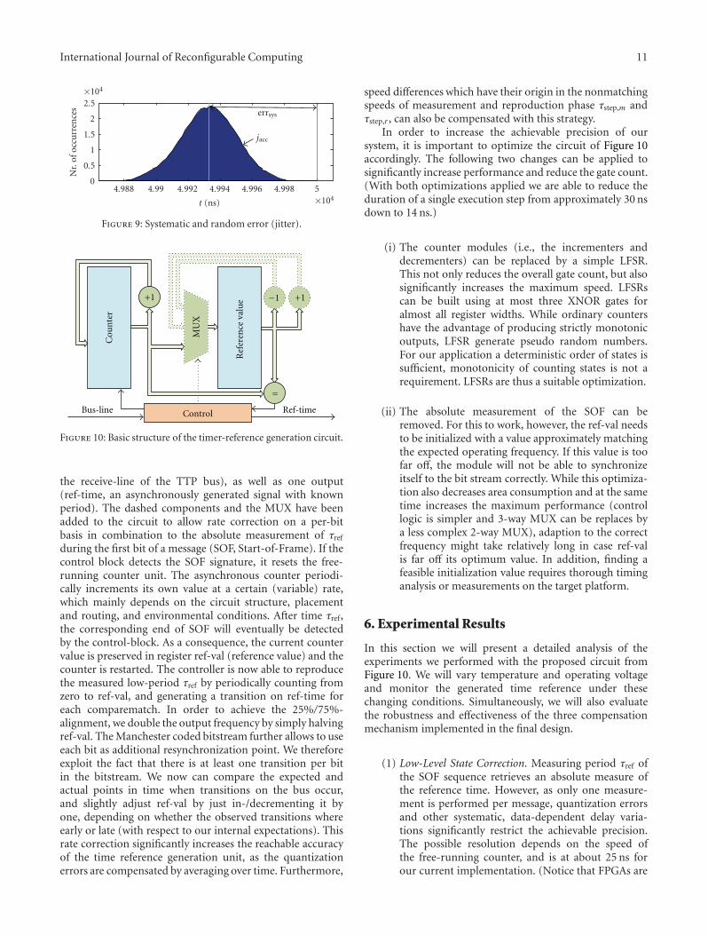
Out of these properties, the following essential con-sequences are derived. The overall systematic error canbe written as errsys = errquant + (1 − fdev)cntrefτstep,m =errquant + cntref(τstep,m − τstep,r). While fdev is almost con-stant for a given circuit, errquant can be different for eachmeasurement (thus errsys is variable as well). Furthermore,long-term accumulated jitter (by definition indeterministicand unbounded) causes additional frequency-inaccuracies.Assuming a normal distribution for jitter induced in everyexecution step, the accumulated jitter can be approximatedas jacc = N(0, σ2

acc) with σ2acc = cntrefσ2

step (where σ2step is the

variance of a single execution step).Figure 9 illustrates the above types of error. A signal with

a high-period of 100μs serves as reference for the generationof a 50μs time-base (solid line on the very right). Thereproduced signal is measured and plotted as jitter histogram(Gaussian-like area). errsys is the deviation of the averagesignal-period from its nominal value at 50μs. On the otherhand, jacc manifests as Gaussian jitter with variance σ2

accaround the mean duration of approximately 49.93μs.

5.3. Implementation. The basic structure of the circuit isshown in Figure 10. As one can see, the interface of ourdesign is quite simple. There is only one input (bus-line,


×10454.9984.9964.9944.9924.994.988

t (ns)

0

0.5

1

1.5

2

2.5×104

Nr.

ofoc

curr

ence

s errsys

jacc

Figure 9: Systematic and random error (jitter).

Cou

nte

r

MU

X

Control

=

+1

Ref

eren

ce v

alu

e

Bus-line Ref-time

−1 +1

Figure 10: Basic structure of the timer-reference generation circuit.

the receive-line of the TTP bus), as well as one output(ref-time, an asynchronously generated signal with knownperiod). The dashed components and the MUX have beenadded to the circuit to allow rate correction on a per-bitbasis in combination to the absolute measurement of τref

during the first bit of a message (SOF, Start-of-Frame). If thecontrol block detects the SOF signature, it resets the free-running counter unit. The asynchronous counter periodi-cally increments its own value at a certain (variable) rate,which mainly depends on the circuit structure, placementand routing, and environmental conditions. After time τref,the corresponding end of SOF will eventually be detectedby the control-block. As a consequence, the current countervalue is preserved in register ref-val (reference value) and thecounter is restarted. The controller is now able to reproducethe measured low-period τref by periodically counting fromzero to ref-val, and generating a transition on ref-time foreach comparematch. In order to achieve the 25%/75%-alignment, we double the output frequency by simply halvingref-val. The Manchester coded bitstream further allows to useeach bit as additional resynchronization point. We thereforeexploit the fact that there is at least one transition per bitin the bitstream. We now can compare the expected andactual points in time when transitions on the bus occur,and slightly adjust ref-val by just in-/decrementing it byone, depending on whether the observed transitions whereearly or late (with respect to our internal expectations). Thisrate correction significantly increases the reachable accuracyof the time reference generation unit, as the quantizationerrors are compensated by averaging over time. Furthermore,

speed differences which have their origin in the nonmatchingspeeds of measurement and reproduction phase τstep,m andτstep,r , can also be compensated with this strategy.

In order to increase the achievable precision of oursystem, it is important to optimize the circuit of Figure 10accordingly. The following two changes can be applied tosignificantly increase performance and reduce the gate count.(With both optimizations applied we are able to reduce theduration of a single execution step from approximately 30 nsdown to 14 ns.)

(i) The counter modules (i.e., the incrementers anddecrementers) can be replaced by a simple LFSR.This not only reduces the overall gate count, but alsosignificantly increases the maximum speed. LFSRscan be built using at most three XNOR gates foralmost all register widths. While ordinary countershave the advantage of producing strictly monotonicoutputs, LFSR generate pseudo random numbers.For our application a deterministic order of states issufficient, monotonicity of counting states is not arequirement. LFSRs are thus a suitable optimization.

(ii) The absolute measurement of the SOF can beremoved. For this to work, however, the ref-val needsto be initialized with a value approximately matchingthe expected operating frequency. If this value is toofar off, the module will not be able to synchronizeitself to the bit stream correctly. While this optimiza-tion also decreases area consumption and at the sametime increases the maximum performance (controllogic is simpler and 3-way MUX can be replaces bya less complex 2-way MUX), adaption to the correctfrequency might take relatively long in case ref-valis far off its optimum value. In addition, finding afeasible initialization value requires thorough timinganalysis or measurements on the target platform.

6. Experimental Results

In this section we will present a detailed analysis of theexperiments we performed with the proposed circuit fromFigure 10. We will vary temperature and operating voltageand monitor the generated time reference under thesechanging conditions. Simultaneously, we will also evaluatethe robustness and effectiveness of the three compensationmechanism implemented in the final design.

(1) Low-Level State Correction. Measuring period τref ofthe SOF sequence retrieves an absolute measure ofthe reference time. However, as only one measure-ment is performed per message, quantization errorsand other systematic, data-dependent delay varia-tions significantly restrict the achievable precision.The possible resolution depends on the speed ofthe free-running counter, and is at about 25 ns forour current implementation. (Notice that FPGAs are


not in any way optimized for LEDR circuits. Dual-rail encoding introduces not only considerable inter-connect delays, but also significant area overheadcompared to ordinary synchronous logic.)

(2) Low-Level Rate Correction. As the Manchester codealways provides a signal transition at 50% of τbit,we can continuously adapt the measured referencevalue ref-val. We only allow small changes to ref-val: It is either incremented or decremented by one,depending on whether the expected signal transitionsare late or early, respectively. The advantage of thisadditional correction mechanism is that quantizationerrors and data-dependent effects are averaged overtime, thus increasing precision.

(3) High-Level Rate Correction. The softwarestack con-trolling the message transmission unit can addanother level of rate correction. As it knows theexpected (from the MEDL) and actual (from thetransceiver unit) arrival times of messages, the dif-ference of both can be used to calculate an error-term. High-level services and message transmissioncan in turn be corrected by this term to achieve evenbetter precision. The maximum resolution which canbe achieved by this technique depends on the baud-rate, and is half a bit-time.

Remark. We are well aware that the presented results canonly be seen as snapshot for our specific setup and technol-ogy. Changing the execution platform will certainly changethe specific outcomes of the measurements, as jitter and thecorresponding frequency instabilities mainly depend on thecircuit structure and the used technology. However, froma qualitative point of view, our results are valid for otherplatforms and technologies as well. The presented modeland the proposed circuits are flexible enough to be appliedto different technologies. However, the main problem isthe necessity to perform concrete measurements for eachtarget technology in order to obtain meaningful quantitativeevaluations. Temporal behavior and specific jitter character-istics are always dependent on fabrication variations and theoperating environment. While the theoretical model needs tobe complemented by thorough measurements, the proposedcircuits are capable of tolerating these (statistical) variationsbecause of the continuous calibration of internal timing.

6.1. Time Reference Generator. Before we start with themessage transmission unit, which implements all of theabove compensation mechanisms, we want to take a closerlook at the basic building block (cf. Figure 10). Clearly,compensation method (3) is not present, as we just inves-tigate the time reference generation unit. This unit doesnot actually receive or transmit messages, it just generatessignal ref-time out of the incoming signal transitions onthe TTP bus. The measurement setup is fairly simple.There is a (synchronous) sender, which periodically sendsManchester coded messages. The asynchronous design usesthese messages to generate its internal time-reference. Allmeasurements have been taken while the bus was idle. This

10010−210−410−610−8

τ (s)

10−14

10−12

10−10

10−8

10−6

10−4

10−2

Alla

n-v

aria

nce

(Hz)

Capture-doneTime-reference

Figure 11: Allan-Variance.

way, we can observe the circuit’s capability of reproducingthe measured duration without any disturbing state- or ratecorrection effects. If not stated otherwise, the measurementsare taken at ambient temperature and nominal supplyvoltage.

First we take a look at the frequency stability of ref-timeand cDone. The first part of the Allan-plot in Figure 11,ranging from approximately 2 ∗ 10−8 s to 10−4 s on thex-axis, is obtained by monitoring the handshaking signalcapturedone from a register cell. The second part, which startsat 3∗ 10−6 s and thus slightly overlaps with capturedone, hasbeen obtained by measuring ref-time. Notice that it is nocoincidence that both parts in the figure almost match inthe overlapping section: Signal ref-time is based upon theexecution of the low-level hardware and is therefore directlycoupled to the respective jitter and stability characteristics.It is obvious from the graph that the stability increases toabout 10−10 Hz for τ ≈ 10−2 s. Furthermore, the referencesignal is far more stable than the underlying generation logic(cDone), as periodically executing the same operations com-pensates data-dependent jitter and averages random jitter.Although the underlying low-level signals jitter considerablydue to data-dependent jitter, the circuit’s output is orders ofmagnitudes more stable, as these variations are canceled outduring the periodic executions.

One of the major benefits of the proposed solution isits robustness to changing operating conditions, thus weadditionally vary the environment temperature and observethe changes in the period of ref-time. We heat the systemfrom room temperature to about 83◦C, and let it cool downagain. Figure 12 compares ref-val to the signal period ofref-time. While the ambient temperature increases, ref-valsteadily decreases from 265 down to 256. The period of ref-time makes an approximately 19 ns-step (the duration ofa single execution step) each time ref-val changes. Duringthe periods where the changes in execution speed cannot becompensated (because they are too small), ref-time slowlydrifts away from the optimum at 5μs. Without any com-pensation measures the duration of ref-time would be about5180 ns at the maximum temperature, instead of being in therange of approximately 5μs ± 38 ns (i.e., the duration of ±two execution steps), no matter what temperature. Notice


300025002000150010005000

Time (s)

256

258

260

262

264

266

LFSR

inde

x

(a)

300025002000150010005000

Time (s)

4.96

4.98

5

5.02

Ref

eren

cedu

rati

on(n

s)

(b)

Figure 12: ref-val versus timer reference period for tempera-turetests.

that the performance of the self-timed circuit decreases by3.5% at the maximum temperature, which seems to berelatively low, but it certainly is a showstopper for reliableTTP communication.

Far more pronounced delay variations can be obtained bychanging the core supply voltage. We applied 0.8 V to 1.68 Vin steps of 20 mV core voltage to our FPGA-board. Thistime the execution speed of our self-timed circuit increasedfrom about 80 ns per step to approximately 15 ns per step,as shown in Figure 13(b). This plot illustrates the jitter his-togram on the y-axis versus the FPGA’s core supply voltageon the x-axis. Thereby, the densities of the histogram arecoded in gray-scale (the darker the denser the distribution).It is evident from the figure that performance increasesexponentially with the supply voltage. This illustration alsoshows other interesting facts. For one, almost all voltageshave at least two separate humps in their histograms. Theseare caused by data-dependencies that originate in the dif-ferent phases ϕ0,1. Furthermore, for low voltages, additionalpeaks appear in the histograms and the separations betweenthe phases increase as well. This can be explained as data-dependent effects caused by different delays through logicstages that are magnified while the circuit slows down. Thisproperty is better illustrated in Figure 13(a), where cycle-to-cycle execution jitter is plotted over the supply voltage. Thegraph appears almost symmetrically along the x-axis, whichis caused by the continuous alternation of phases.

We conclude that varying operating conditions not onlyaffect the speed of asynchronous circuits, but also the respec-tive jitter characteristics. In this perspective, slower circuitstend to have higher jitter, which is further magnified byincreased quantization errors due to the low sampling rate.

6.2. Transceiver Unit. The message transmission unit willimplement all three compensation methods mentioned atthe beginning of Section 6. We intend to use this unit directlyin the envisioned asynchronous TTP controller, thus weneed to examine the gained precision of this design withrespect to timeliness. The interface from the controlling(asynchronous) host to the subdesign of Section 6.1 isrealized as dual-ported RAM: Whenever the bus transceiverreceives a message, it stores the payload in combination withthe receive-timestamp in RAM and issues a receive-interrupt(we define the internal time to be the number of ticks ofsignal ref-time, i.e., the number of execution steps performedby the bus transceiver unit). Likewise, the host can request totransfer messages by writing the payload and the estimatedsending time into RAM and asserting the transmit request.

During reception of messages, the circuit can continu-ously recalibrate itself to the respective baud rate, as Manch-ester code provides at least one signal transition per bit.However, between messages and during the asynchronousnode’s sending slot, resynchronization is not possible. Inthese phases we need to rely on the correctness of ref-time. The Start-Of-Frame sequence of each message must beinitiated during a relatively tight starting window, which isslightly different for all nodes and is continuously adaptedby the TTP’s distributed clock synchronization algorithm.Failing to hit this starting window is an indication that thenode is out-of-sync.

As we are interested in the accuracy of hitting thestarting window, we configured the controlling host in away that it triggers a message-transmission 25 bit-times afterthe last bit of an incoming message. We simultaneouslyheated the system from room temperature to about 68◦Cto check on the expected robustness against the respectivedelay variations. The results are shown in Figure 14, wherethe deviation from the optimal sending-point (in unitsof bit-times) and the operating temperature are plottedagainst time. Similar to Figure 12 one can see that while thecircuit gets warmer (and thus slower), the deviation steadilyincreases. As soon as the accumulated changes in delay canbe compensated by the low-level measurement circuitry (i.e.,ref-val decreases), the mean deviation immediately jumpsback to about zero. We can see in the figure that the timingerror is in the range from approximately −0.1 to +0.2 bit-times, which will surely satisfy the needs of TTP.

The next property we are interested in is the circuit’sbehavior with respect to different baud rates. Although lowbitrates have the advantage of minimizing the quantizationerror, jitter has much more time to accumulate comparedto high data rates. It is thus not necessarily true that lowerbaud rates result in a more stable and precise time reference.On the other hand, if the data rate is too high, it is notpossible to reproduce τref correctly, and even small changesof the reference value ref-val lead to large relative errorsin the resulting signal period. The optimum baud rate willtherefore be located somewhere between these extremes.Figure 15 illustrates this by plotting the mean deviations ofthe optimum sending points versus the bitrate (the “corri-dor” additionally shows the respective standard deviations).Notice that the y-axis shows the relative deviation in units


1.61.41.210.8

Voltage (V)

15

10

5

0

−5

−10

−15

−20

C2C

jitte

r(n

s)

(a)

1.61.41.210.8

Voltage (V)

90

80

70

60

50

40

30

20

Jitt

erhi

stog

ram

(ns)

(b)

Figure 13: (a) Cycle-to-cycle jitter, (b) jitter histogram.

800070006000500040003000200010000

Time (s/10)

−0.2

−0.1

0

0.1

0.2

0.3

Dev

iati

on(b

itti

mes

)

20

30

40

50

60

70

Tem

per

atu

re(◦

C)

Figure 14: Relative deviation from optimal sending slot andoperating temperature.

25020010075502010521

Baudrate (kHz)

−0.6

−0.4

−0.2

0

0.2

0.4

0.6

0.8

Dev

iati

on(b

itti

mes

)

Figure 15: Mean relative deviation from optimal sending pointversus baud rate.

of bit-times. Therefore, for example, the absolute deviationof the 1 kHz bit-rate is more than 50 times larger than thatof 50 kHz. Clearly, TTP does not support baud rates aslow as 1 kHz. Reasonable data rates are at least at 100 kHz

25020010075502010521

Baudrate (kHz)

−0.08

−0.06

−0.04

−0.02

0

0.02

Rel

ativ

ede

viat

ion

(bit

tim

es)

−5

0

5

10

15

20×10−7

Abs

olu

tede

viat

ion

(s)

Relative deviationAbsolute deviation

Figure 16: Mean relative/absolute deviation from optimum bit-time.

and above (up to 4 Mbit/s for Manchester coding). Ourcurrent setup allows us to use 100 kbit/s for communicationwith acceptable results. However, we hope to be able toachieve 500 kbit/s in our final system setup (with a moresophisticated development platform and a further optimizeddesign).

Finally, we take a look at the accuracy of the generatedtime reference for different baud rates. Figure 16 thereforeshows the mean relative (again in units of bit-times) andthe absolute (in seconds) deviations of the actual referenceperiods from their nominal values. For all baud rates, therelative deviations are within a range of approximately±0.01bit-times, or ±1%, while the absolute timing errors aresignificantly larger for baud rates below 50 kbit/s.


7. Conclusion

In this paper we introduced the research project ARTS,provided information on the project goals and explainedthe concept of TTP. We proposed a method of using TTP’sbit stream to generate an internal time reference (whichis needed for message transfer and most high-level TTPservices). With this transceiver unit for Manchester codedmessages we performed measurements under changing oper-ating temperatures and voltages. The results clearly show thatthe proposed architecture works properly. The results furtherindicate that the achievable precision is in the range ofabout 1%. This is not a problem while other (synchronous)nodes are transmitting messages, as resynchronization canbe performed continuously. However, during message trans-mission of our node, the design depends on the quality of thegenerated reference time. Our measurement show that we areable to hit the optimum sending point with a precision ofapproximately ±0.3 bit-times (assuming an interframe gapof 25 bits), which should be enough for the remaining nodesto accept the messages.

The presented approach is of course not only limitedto TTP, although it clearly is optimized for TTP’s uniqueproperties. For instance, receiver and transmitter modulesfor all kinds of asynchronous serial protocols (e.g., UART)can be implemented using our solution. The important—and probably limiting—part is, independently of the appli-cation, to find suitable resynchronization points or patterns.While these are provided by TTP on a periodic, regular andfixed basis, a start-bit of defined length or a special bit patterncould be used for other communication protocols. Generallyspeaking, self-timed or (Q)DI asynchronous circuits aredifficult to use if strictly timed actions need to be performed,because there are no events of defined duration available.With our approach, however, a basic notion of time can beestablished even in the absence of a highly stable clock signal.

There still is much work to be done. The presented tem-perature and voltage tests are only a relatively small subsetof tests that can be performed. One of the most interestingquestions concerns the dynamics of changing operating con-ditions. How rapidly and aggressively can the environmentchange for the asynchronous TTP controller to still maintainsynchrony with the remaining system? It should be clearfrom our approach that an answer to this question canonly be given with respect to the concrete TTP schedule, asmessage lengths, interframe gaps, baud rate, and so forth.directly influence the achievable precision of our solution.The next steps of the project plan include the integrationof the presented transceiver unit into an asynchronousmicroprocessor, the implementation of the correspondingsoftware stack, and the interface to the (external) applicationhost controller. Once the practical challenges are finished,thorough investigations of precision, reliability and robust-ness of our asynchronous controller will be performed.

Acknowledgment

The ARTS project receives funding from the FIT-IT programof the Austrian Federal Ministry of Transport, Innovation

and Technology (bm:vit, http://www.bmvit.gv.at/), projectno. 813578.

References

[1] C. J. Myers, Asynchronous Circuit Design, John Wiley & Sons,New York, NY, USA, 2001.

[2] J. Sparso and S. Furber, Principles of Asynchronous CircuitDesign—A Systems Perspective, Kluwer Academic Publishers,Boston, Mass, USA, 2001.

[3] N. Miskov-Zivanov and D. Marculescu, “A systematicapproach to modeling and analysis of transient faults in logiccircuits,” in Proceedings of the 10th International Symposiumon Quality Electronic Design (ISQED ’09), pp. 408–413, March2009.

[4] H. Kopetz and G. Grundsteidl, “TPP—a time-triggered proto-col for fault-tolerant real-time systems,” in Proceedings of the23rd International Symposium on Fault-Tolerant Computing(FTCS ’93), pp. 524–533, June 1993.

[5] H. Kopetz, Real-Time Systems: Design Principles for DistributedEmbedded Applications, Kluwer Academic Publishers, Boston,Mass, USA, 1997.

[6] AS8202NF—TTP-C2NF Communication Controller, TTTechComputertechnik AG, Revision 2.1 edition, http://www.austriamicrosystems.com/.

[7] M. E. Dean, T. E. Williams, and D. L. Dill, “Efficient self-timing with level-encoded 2-phase dual-rail (LEDR),” in Pro-ceedings of the University of California/Santa Cruz Conferenceon Advanced Research in VLSI, pp. 55–70, MIT Press, 1991.

[8] A. J. McAuley, “Four state asynchronous architectures,” IEEETransactions on Computers, vol. 41, no. 2, pp. 129–142, 1992.

[9] D. H. Linder and J. C. Harden, “Phased logic: supportingthe synchronous design paradigm with delay-insensitive cir-cuitry,” IEEE Transactions on Computers, vol. 45, no. 9, pp.1031–1044, 1996.

[10] K. M. Fant and S. A. Brandt, “NULL Convention LogicTM:a complete and consistent logic for asynchronous digitalcircuit synthesis,” in Proceedings of International Conferenceon Application-Specific Systems, Architectures and Processors(ASAP ’96), pp. 261–273, Chicago, Ill, USA, August 1996.

[11] M. Ferringer, “Coupling asynchronous signals into asyn-chronous logic,” in Proceedings of the 17th Austrian Workshopon Microelectronics (Austrochip ’09), Graz, Austria, October2009.

[12] M. Simlastik and V. Stopjakova, “Automated synchronous-to-asynchronous circuits conversion: a survey,” in IntegratedCircuit and System Design. Power and Timing Modeling,Optimization and Simulation, vol. 5349 of Lecture Notes inComputer Science, pp. 348–358, 2009.

[13] J. Lechner, Implementation of a design tool for generation of FSLcircuits, M.S. thesis, Technische Universitat Wien, Institut furTechnische Informatik, Vienna, Austria, 2008.

[14] Maxim-IC, “Microcontroller Clock-Crystal, Resonator, RCOscillator, or Silicon Oscillator?” application Note 2154, 2003,http://www.maximic.com/appnotes.cfm/an pk/2154.

[15] F. Bala and T. Nandy, “Programmable high frequency RCoscillator,” in Proceedings of the 18th International Conferenceon VLSI Design: Power Aware Design of VLSI Systems, pp. 511–515, January 2005.

[16] A. J. Winstanley, A. Garivier, and M. R. Greenstreet, “Anevent spacing experiment,” in Proceedings of InternationalSymposium on Asynchronous Circuits and Systems, pp. 47–56,Manchester, UK, April 2002.


[17] S. Fairbanks and S. Moore, “Analog micropipeline rings forhigh precision timing,” in Proceedings of the InternationalSymposium on Advanced Research in Asynchronous Circuits andSystems, vol. 10, pp. 41–50, April 2004.

[18] M. Ferringer, G. Fuchs, A. Steininger, and G. Kempf, “VLSIimplementation of a fault-tolerant distributed clock genera-tion,” in Proceedings of the 21st IEEE International Symposiumon Defect and Fault Tolerance in VLSI Systems (DFT ’06), pp.563–571, Arlington, Va, USA, October 2006.

[19] S. Fairbanks and S. Moore, “Self-timed circuitry for globalclocking,” in Proceedings of the 11th IEEE International Sympo-sium on Asynchronous Circuits and Systems (ASYNC ’05), pp.86–96, March 2005.

[20] V. Zebilis and C. P. Sotiriou, “Controlling event spacing in self-timed rings,” in Proceedings of the 11th IEEE International Sym-posium on Asynchronous Circuits and Systems (ASYNC ’05), pp.109–115, March 2005.

[21] J. Ebergen, S. Fairbanks, and I. Sutherland, “Predictingperformance of micropipelines using charlie diagrams,” inProceedings of the 4th International Symposium on AdvancedResearch in Asynchronous Circuits and Systems, pp. 238–246,San Deigo, Calif, USA, March-April 1998.

[22] Tektronix, “Understanding and Characterizing Timing Jitter,”2003.

[23] M. Shimanouchi, “An approach to consistent jitter modelingfor various jitter aspects and measurement methods,” inProceedings of International Test Conference, pp. 848–857,Baltimore, Md, USA, October-November 2001.

[24] I. Zamek and S. Zamek, “Definitions of jitter measurementterms and relationships,” in Proceedings of IEEE InternationalTest Conference (ITC ’05), pp. 25–34, November 2005.

[25] D. W. Allan, N. Ashby, and C. C. Hodge, The Science ofTimekeeping, application Note 1289, 1997, http://www.allanstime.com/Publications/DWA/Science Timekeeping/TheScienceOfTimekeeping.pdf.

[26] D. A. Howe, “Interpreting oscillatory frequency stabilityplots,” in Proceedings of the IEEE International FrequencyControl Symposium and PDA Exhibition, pp. 725–732, May2002.

[27] B. Butka and R. Morley, “Simultaneous switching noise andsafety critical airborne hardware,” in Proceedings of IEEESoutheastcon, pp. 439–442, March 2009.

International Journal of

AerospaceEngineeringHindawi Publishing Corporationhttp://www.hindawi.com Volume 2010

RoboticsJournal of

Hindawi Publishing Corporationhttp://www.hindawi.com Volume 2014


Active and Passive Electronic Components

Control Scienceand Engineering

Journal of



RotatingMachinery


Hindawi Publishing Corporation http://www.hindawi.com

Journal ofEngineeringVolume 2014

Submit your manuscripts athttp://www.hindawi.com

VLSI Design



Shock and Vibration


Civil EngineeringAdvances in

Acoustics and VibrationAdvances in



Electrical and Computer Engineering

Journal of

Advances inOptoElectronics

Hindawi Publishing Corporation http://www.hindawi.com

Volume 2014

The Scientific World JournalHindawi Publishing Corporation http://www.hindawi.com Volume 2014

SensorsJournal of


Modelling & Simulation in EngineeringHindawi Publishing Corporation http://www.hindawi.com Volume 2014


Chemical EngineeringInternational Journal of Antennas and

Propagation




Navigation and Observation



DistributedSensor Networks


On Self-Timed Circuits in Real-Time Systems

Documents

Transcript of On Self-Timed Circuits in Real-Time Systems