On parametrized linear systems, moments, eigenvalues, gradients, and Krylov...

On parametrized linear systems, moments, eigenvalues,gradients, and Krylov methods

Karl Meerbergen

K.U. Leuven

WSC Spring Meeting — Antwerp

On parametrized linear systems, moments, eigenvalues,gradients, and Krylov methods

Karl Meerbergen

K.U. Leuven

WSC Spring Meeting — Antwerp

Collaborators:

Zhaojun Bai

Yao Yue

Maryam Saadvandi

Jeroen De Vlieger

Elias Jarlebring

Wim Michiels

Outline

1 Motivation

2 Overview of methodsModal truncationVector-Pade approximationFrequency sweepingInput/output MOR

3 Lanczos method

4 Nonlinear frequency dependence

5 Multiple right-hand sides

6 Gradients

7 Conclusions

Karl Meerbergen (K.U. Leuven) Parameterized linear systems WSC@UA - May 3rd, 2010 2 / 48

Examples of vibrating systems

Car tyres



Car tyres

Windscreens

Structural damping Choice of connection (glue) to the car



Planes



Planes

Bridge vibrating under footsteps and Thames wind



Maxwell-equation – electrical circuits



Maxwell-equation – electrical circuits

micro-gyroscope for navigation systems


Fourier analysis of finite element model

(K + iωC − ω2M)x = f

f and x : vectors of length n

K , C and M : n × n sparse matrices. In real applications n variesfrom 103 to over 106.

x is called the frequency response function.

Compute x for ω = ω1, . . . , ωp ∈ Ω = [ωmin, ωmax].


Acoustic industrial applications : vibro-acoustics

vibrating structure (modelized by structural modes)

acoustic domain (finite elements)

acoustic radiation towards infinity (infinite elements)

structure is modelized by ‘modes’ (eigen functions)


Traditional frequency response computation

1. For ω = ω1, . . . , ωp

1.1. Solve the linear system (K + iωC − ω2M)x = f for x

For each frequency, a large system of algebraic equations needs to besolved.This requires a linear solver for a large sparse matrix.

For a direct solver (based on LU factorization): a sparse matrix factorization LU = K − ω2M + iωC (expensive) and a backward solve LUx = f (relatively cheap).


Traditional frequency response computation

1. For ω = ω1, . . . , ωp

1.1. Solve the linear system (K + iωC − ω2M)x = f for x

For each frequency, a large system of algebraic equations needs to besolved.This requires a linear solver for a large sparse matrix.

For a direct solver (based on LU factorization): a sparse matrix factorization LU = K − ω2M + iωC (expensive) and a backward solve LUx = f (relatively cheap).

The goal is to reduce the number of matrix factorizations.


Linear system solvers

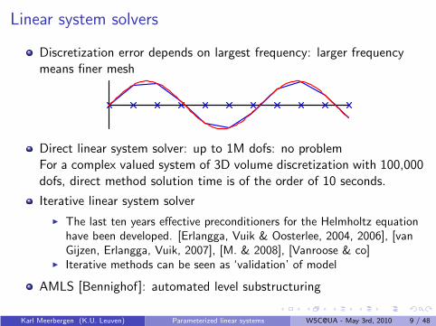
Discretization error depends on largest frequency: larger frequencymeans finer mesh


Linear system solvers

Discretization error depends on largest frequency: larger frequencymeans finer mesh

Direct linear system solver: up to 1M dofs: no problemFor a complex valued system of 3D volume discretization with 100,000dofs, direct method solution time is of the order of 10 seconds.

Iterative linear system solver

The last ten years effective preconditioners for the Helmholtz equationhave been developed. [Erlangga, Vuik & Oosterlee, 2004, 2006], [vanGijzen, Erlangga, Vuik, 2007], [M. & 2008], [Vanroose & co]

Iterative methods can be seen as ‘validation’ of model

AMLS [Bennighof]: automated level substructuring


Overview of methods

Consider(K − ω2M)x = f

with

K and M large sparse, real symmetric matrices

M positive definite

f independent of ω: typically point loads

Three basic methods:

Modal truncation

Pade approximation

Mixed direct iterative procedure (fast frequency sweeping)


Modal truncation

Consider the eigendecomposition

Kuj = λjMuj

The solution of (K − ω2M)x = f is

x =n

∑

j=1

uj

uTj f

λj − ω2

Rational function with poles λj .


Modal superposition, cont.

x =n

∑

j=1

uj

uTj f

λj − ω2≈

k∑

j=1

uj

uTj f

λj − ω2

0.01

0.1

1

10

100

1000

0 2 4 6 8 10 12

"undamped""undamped10""undamped7"


Vector-Pade approximation

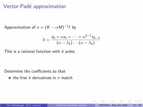
Approximation of x = (K − αM)−1f by

x =x0 + αx1 + · · · + αk−1xk−1

(α − λ1) · · · (α − λk)

This is a rational function with k poles.

Determine the coefficients so that

the first k derivatives in σ match


Frequency sweeping

For each ω precondition

(K − ω2M)x = f

into(K − σM)−1(K − ω2M)x = (K − σM)−1f

and solve by an iterative method.

Use linear system solver for applying (K − σM)−1

For the AMLS method, K − σM is a diagonal matrix.


Input-output system

SISO

(K − ω2M)x = b

y = dT x

Compute y accurately and fast

Use MOR as fast solver

Often many outputs (100’s or 1000’s)

Twosided methods (MOR) are not often used in this case


Summary

Modal truncation:

x =k

∑

j=1

uj

uTj f

λj − α

Pade approximation:

x =x0 + αx1 + · · · + αk−1xk−1

(α − µ1) · · · (α − µk)

Frequency sweepingSolve (M − ω2M)x = f by an iterative method

MOR: find reduced model for linear system

(K − ω2M)x = b

y = dT x


Numerical example: BMW Windscreen

Glaverbel-BMW windscreenwith 10% structural damping

Direct method : 2653 seconds

Lanczos method : 14 seconds

1e-05

0.0001

0.001

0.01

0.1

1

10

0 20 40 60 80 100 120 140 160 180 200


Notation

Define α = ω2

A = (K − σM)−1M and b = (K − σM)−1f

Assume σ = 0 and

then we solve(K − αM)x = f

or

(K − σ)−1(K − αM)x = (K − σ)−1f

(I − αA)x = b

Eigenvalue problem:Kuj = λjMuj

Assume A symmetric.


Lanczos method

Krylov space: spanb, Ab, . . . ,Ak−1b

Lanczos method builds orthogonal basis Vk = [v1, . . . , vk ].

Range(Vk) = spanb, Ab, . . . ,Ak−1b

and a tridiagonal matrix Tk = V Tk AVk

major cost: k matrix vector products with A : w = Av

small cost when k is small

Also called Ritz vector technique (mechanical engineering)


Lanczos method

Transform a large size matrix into a small size matrix

Tk = V Tk A Vk


Shift-invariance property

Krylov spacesv , Av , A2v , . . .

andv , (I − αA)v , (I − αA)2v , . . .

are equal, since (I − αA)v = v − αAv

Applying the Lanczos method to A, applies it for free to A + αI for allα.


Shift-invariance property

Krylov spacesv , Av , A2v , . . .

andv , (I − αA)v , (I − αA)2v , . . .

are equal, since (I − αA)v = v − αAv

Applying the Lanczos method to A, applies it for free to A + αI for allα.

As, a consequence,

V Tk AVk = Tk

V Tk (I − αA)Vk = I − αTk

Therefore, no need to build Krylov space for different values of α


Shifted or parameterized linear systems

Analyzed in the context of model reduction methods (Connectionwith rational approximation)[Gallivan, Grimme, Van Dooren 1994], [Feldman, Freund 1995], [Gallivan,

Grimme, Van Dooren 1996], [Grimme, Sorensen, Van Dooren 1996], [Ruhe &

Skoogh 1998], [Bai & Freund 2000], [Bai & Freund 2001] [Bai & Su 2006]

in the context of parameterized linear systems[Freund 1993], [Frommer & Glassner, 1993], [Simoncini & Gallopoulos

1998], [Simoncini, 1999, 2010], [Simoncini & Perotti 2002], [M. 2003],

[Edema, Vuik 2008], [M. 2008], [M. & Bai, 2010]


Undamped vibration problem

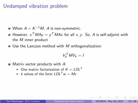
When A = K−1M, A is non-symmetric.

However, xTMAy = yTMAx for all x , y . So, A is self-adjoint withthe M inner product

Use the Lanczos method with M orthogonalization:

V Tk MVk = I

Matrix vector products with A: One matrix factorization of K = LDLT

k solves of the form LDLTw = Mv


Iterative solver connection

Lanczos method (Conjugate gradients) is iterative linear system solverfor

(I − αA)x = b

Let A = K−1M

Let Kuj = λjMuj

Eigenvalues of K−1(K − ω2M) are θj =λj − ω2

λj

Fast convergence when most eigenvalues are clustered around one: ω close to 0

λj θj

0 ω20 1

When there are no eigenvalues λ between 0 and ω2, then we have apositive definite linear system


MINRES versus Lanczos

Lanczos:x =

∑ yj

α − µj

Vertical asymptotes


MINRES versus Lanczos

Lanczos:x =

∑ yj

α − µj

Vertical asymptotes

MINRES:

x =∑ yj(α)

α − µj(α)

Denominator is never zero No vertical asymptotes


Example

0 20 40 60 80 100 120 140 160 180 200

LanczosMINRES

10−1

10−2

10−3

10−4

10−5

10−6

10−7

10−8

10−


Eigenvalue and Pade connection

Lanczos method produces k eigenvalue estimates: eigenvalues of Tk

We can show that the Lanczos method computes

x =k

∑

j=1

uj

wTj f

λj − α

where uj is a Ritz vector (i.e. approximate eigenvector).

There are k terms, so we can only compute k vertical asymptotes inthe function

The number of eigenvalues in the frequency range should be smallerthan k.


Eigenvalue and Pade connection

Lanczos method produces k eigenvalue estimates: eigenvalues of Tk

We can show that the Lanczos method computes

x =k

∑

j=1

uj

wTj f

λj − α

where uj is a Ritz vector (i.e. approximate eigenvector).

There are k terms, so we can only compute k vertical asymptotes inthe function

The number of eigenvalues in the frequency range should be smallerthan k.

Pade connection: x is a rational approximation with

x (j)(0) = x (j)(0) for j = 0, . . . , k − 1


Eigenvalue connection: example

Hard problem: more than10,000 eigenvalues

Easy problem: less than 20eigenvalues


Industrial example with NASTRAN

Traditional computation For each frequency, perform factorization of K − ω2M and solve

Lanczos computation One matrix factorization of K − σM and solve k solves.


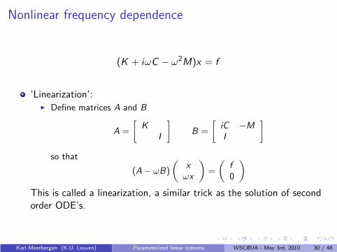
Nonlinear frequency dependence

(K + iωC − ω2M)x = f

‘Linearization’: Define matrices A and B

A =

[

K

I

]

B =

[

iC −M

I

]

so that

(A − ωB)

(

x

ωx

)

=

(

f

0

)

This is called a linearization, a similar trick as the solution of secondorder ODE’s.


Linearizations

Linearizations have been studied for the solution of the quadraticeigenvalue problem

(K + λC + λ2M)u = 0

[Gohberg, Lancaster, Rodman, 1982] [Tisseur, M. 2001][Mackey,Mackey,Mehl,Mehrmann,2006]

Methods based on Companion ‘linearization’

Higher order polynomials

(A0 + ωA1 + · · · + Apωp)x = f

Transform to

A0

−I

. . .

−I

+ ω

A1 A2 · · · Ap

I 0

. . .. . .

I 0

x

ωx

.

.

.ω

p−1x

=

f

0...0


Methods

[Parlett & Chen 1990] Pseudo Lanczos method (pretends B ispositive definite)

[Simoncini & al, 2005] similar

[Freund, 2005]: analysis of Krylov spaces

[Bai & Su, 2005] SOAR: based on Arnoldi’s method

[M. 2008] Q-Arnoldi: based on Arnoldi’s method (for eigenvalueproblems)

[Amiraslani, Corless, Lancaster, 2009] Other polynomials than powersof ω.

[Jarlebring, M., Michiels 2010] Infinite-Arnoldi: based on Arnoldi’smethod (for delay eigenvalue problem)


Multiple right-hand sides

(K − ω2M)[x1, . . . , xs ] = [f1, . . . , fs ]

for ω ∈ Ω = [ωmin, ωmax].Methods:



(K − ω2M)[x1, . . . , xs ] = [f1, . . . , fs ]


Use Lanczos method for each fj separately Low memory cost The cost is proportional to s



(K − ω2M)[x1, . . . , xs ] = [f1, . . . , fs ]



Use block-Lanczos method for each all fj together Fast method High memory cost



(K − ω2M)[x1, . . . , xs ] = [f1, . . . , fs ]



Use block-Lanczos method for each all fj together Fast method High memory cost

Recycling Ritz vectors in Krylov methods [Giraud,Ruiz & Touhami,2006] [Kilmer & de Sturler 2006] [Darnell, Morgan, Wilcox 2007][Stathopoulos & Orginos, 2009][M. & Bai, 2010]


Recycling

Compute the FRF for the first right-hand side

Extract eigenvalues / eigenvectors

For each remaining right-hand side, reuse of p eigenvectors


Recycling




Methods: (classical) Lanczos method:

x =

k∑

j=1

uj

uTj f

λj − ω2

⋆ First k moments of x and x match.


Recycling




Methods: (classical) Lanczos method:

x =

k∑

j=1

uj

uTj f

λj − ω2

⋆ First k moments of x and x match.

With reuse of eigenvalues:

x =

p∑

j=1

uj

uTj f

λj − ω2+

k∑

j=p+1

uj

uTj f

λj − ω2

⋆ First k − p moments of x and x match.⋆ Interpolation in the p deflated eigenvalues.


Frequency sweeping with modal acceleration

The solution of(I − ω2A)x = b (1)

for ω ∈ Ω is split into two parts.





Let Up = [u1, . . . , up] be the eigenvectors corresponding to theeigenvalues in Ω2.

Compute

xp =

p∑

j=1

uj

uTj f

λj − ω2





Let Up = [u1, . . . , up] be the eigenvectors corresponding to theeigenvalues in Ω2.

Compute

xp =

p∑

j=1

uj

uTj f

λj − ω2

Solve (1) iteratively using starting vector xp, i.e. x = xp + y with y

the solution of

(I − ω2A)y = b − (I − ω2A)xp

= (I − UpUTp M)b


Modal acceleration

We can prove that eigenvalues in the frequency range are computedto machine precision

As a result, the right-hand side has ‘no’ components in the associatedeigenvalues

This significantly improves the condition number

Eigenvalues of Kx = λMx Eigenvalues of A

ω2min ω2

max 0 1

Most eigenvalues of A lie near one. The number of required iterations is the number of isolated eigenvalues

of A away from one. Convergence for all ω2 ∈ Ω2 requires the number of iterations, k, to be

at least the number of eigenvalues in Ω2. Remove the red eigenvalues: positive definite matrix, and small

condition number


Windscreen

Glaverbel-BMW windscreen

grid : 3 layers of 60 × 30 HEX08 elements (n = 22, 692)

Ω = [0, 100]

First run: unit point force at one of the corners Use Lanczos method with k = 20 vectors. We keep the Ritz values in [0, 2 × 1002] : p = 14


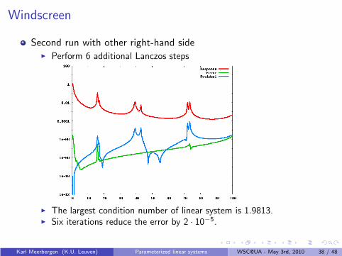
Windscreen

Second run with other right-hand side Perform 6 additional Lanczos steps

The largest condition number of linear system is 1.9813. Six iterations reduce the error by 2 · 10−5.


Acoustic cavity

n = 48, 158

Frequency range : [0, 10000]

202 right-hand sides

matrix factorization: 8 seconds

Lanczos method with 40 vectors: 6 seconds


Acoustic cavity (cont.)

2nd right-hand side: keep the 31 Ritz values in [0, 2 × 10.0002].

9 additional Lanczos iterations recycling 31 Ritz vectors: 2 seconds

0.001

0.01

0.1

1

10

100

1000

0 1000 2000 3000 4000 5000 6000 7000 8000 9000 10000

Exactrecycling

0.001

0.01

0.1

1

10

100

1000

0 1000 2000 3000 4000 5000 6000 7000 8000 9000 10000

Exactk=50

0.001

0.01

0.1

1

10

100

1000

0 1000 2000 3000 4000 5000 6000 7000 8000 9000 10000

Exactk=19

With recycling Lanczos k = 50 Lanczos k = 19


Acoustic cavity

n = 140, 228

Frequency range : [0, 10000]

202 right-hand sides

matrix factorization: 13 seconds

Lanczos method with 50 vectors: 15 seconds

Recycling 36 vectors: only 4 seconds

For 201 right-hand sides: 800 instead of 3000 seconds.


Multiple eigenvalues

3D Laplacian on a cube.

30 Lanczos iterations with first right-hand side

Recycle 22 Ritz pairs

Run 8 iterations with the second right-hand side

0.1

1

10

100

0 2 4 6 8 10 12 14 16 0.001

0.01

0.1

1

10

0 2 4 6 8 10 12 14 16

ExactRecycling

0.001

0.01

0.1

1

10

0 2 4 6 8 10 12 14 16

Exactk=8

Lanczos for f1 Recylcing for f2 Lanczos k = 8 for f2


Gradient computation

Determination of optimal parameters of a vibrating system

Example: optimal parameters for a damper of a floor in a buildingnear a noisy road

m1

c1k1


Optimization problem

Parametrized linear system:

(K (p) + iωC (p) − ω2M(p))x = f

y = dT x

Find parameters p so that ‖y‖2 =

∫

ωmax

0|y |2dω is minimal

‖y‖∞ = supωmax0 |y |2 is minimal

This is, in general, a non-smooth optimization problem

Expensive evaluation of y and the gradient

Model order reduction is an important tool to reduce thecomputational cost

Both function value and gradient should be computed by the reducedmodel


Gradient computation

[Antoulas, Beattie, Gugercin 2010] [Yue, M. 2010] show interpolationproperties on derivatives for two-sided MOR:

(K (p) + iωC (p) − ω2M(p))x = f

y = dT x

Z (ω) = K + iω − ω2M x = Z (ω)−1f y = dT x

∂y

∂p= (Z (ω)−1d)T

∂Z (ω)

∂pZ (ω)−1f

Z (ω)−Td and Z (ω)−1f are computed by two-sided Krylov methods


Numerical example

Floor with damper (n = 29800)

Reduced model k = 25

Determine optimal parameters

Direct method Krylov

Matrix size 29800 25Optimizer computed (14007181,42404) (14007225, 42410)Function value 134.5477989 134.5479496CPU time Several Days 3735s


Conclusions

Krylov methods usually work well for acoustic simulation

Recycling Ritz vectors is a reliable and efficient method for thesolution with multiple right-hand sides

Parametrized models with many parameters are current challenges

Solving parameterized linear systems with multiple right-hand sidescan benefit from recycling Ritz vectors

Does not work well when eigenvalues are multiple

Also works for Rayleigh damping


Bibliography

(Also:www.cs.kuleuven.be/~karlm)

J. De Vlieger and K. Meerbergen.

Analysis and computation of eigenvalues of symmetric fuzzy matrices.In T. Simos, editor, Proceedings of the ICNAAM09 Conference, 2009.

K. Meerbergen.

The solution of parametrized symmetric linear systems.SIAM J. Matrix Anal. Appl., 24(4):1038–1059, 2003.

K. Meerbergen.

Fast frequency response computation for Rayleigh damping.International Journal of Numerical Methods in Engineering, 73(1):96–106, 2008.

K. Meerbergen.

The Quadratic Arnoldi method for the solution of the quadratic eigenvalue problem.SIAM J. Matrix Anal. and Applic., 30(4):1463–1482, 2008.

K. Meerbergen and Z. Bai.

The Lanczos method for parameterized symmetric linear systems with multiple right-hand sides.SIAM J. Matrix Anal. and Applic., 31(4):1642–1662, 2010.

K. Meerbergen and J.P. Coyette.

Connection and comparison between frequency shift time integration and a spectral transformation preconditioner.Numerical Linear Algebra with Applications, 16:1–17, 2009.

F. Tisseur and K. Meerbergen.

The quadratic eigenvalue problem.SIAM Review, 43(2):235–286, 2001.


www.cs.kuleuven.be/~karlm

On parametrized linear systems, moments, eigenvalues, gradients, and Krylov...

Documents

Transcript of On parametrized linear systems, moments, eigenvalues, gradients, and Krylov...