On mathematical programming with indicator constraints · On mathematical programming with...

On mathematical programmingwith indicator constraints

Andrea Lodijoint work with P. Bonami & A. Tramontani (IBM), S. Wiese (Unibo)

University of Bologna, ItalyEcole Polytechnique de Montreal, Quebec, Canada

[email protected]

International Symposium on Mathematical Programming (ISMP 2015)Pittsburgh, July 16, 2015

Andrea Lodi (Bologna U & Polytechnique Montreal) On MP with indicator constraints ISMP 2015 1 / 29

Introduction & Motivation

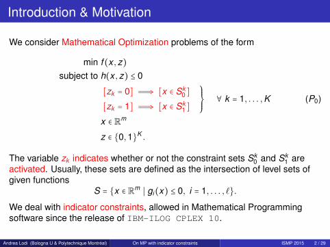
We consider Mathematical Optimization problems of the form

min f (x ,z)subject to h(x ,z) ≤ 0

[zk = 0] Ô⇒ [x ∈ Sk0 ]

[zk = 1] Ô⇒ [x ∈ Sk1 ]

⎫⎪⎪⎬⎪⎪⎭∀ k = 1, . . . ,K (P0)

x ∈ Rm

z ∈ 0,1K .

The variable zk indicates whether or not the constraint sets Sk0 and Sk

1 areactivated. Usually, these sets are defined as the intersection of level sets ofgiven functions

S = x ∈ Rm ∣ gi(x) ≤ 0, i = 1, . . . , `.

We deal with indicator constraints, allowed in Mathematical Programmingsoftware since the release of IBM-ILOG CPLEX 10.


Introduction & Motivation (cont.d)

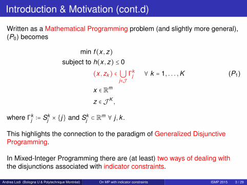
Written as a Mathematical Programming problem (and slightly more general),(P0) becomes

min f (x ,z)subject to h(x ,z) ≤ 0

(x ,zk) ∈ ⋃j∈J

Γkj ∀ k = 1, . . . ,K (P1)

x ∈ Rm

z ∈ J K ,

where Γkj ∶= Sk

j × j and Skj ⊂ Rm ∀ j ,k .

This highlights the connection to the paradigm of Generalized DisjunctiveProgramming.

In Mixed-Integer Programming there are (at least) two ways of dealing withthe disjunctions associated with indicator constraints.


The so-called bigM approach

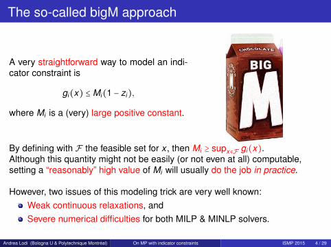
A very straightforward way to model an indi-cator constraint is

gi(x) ≤ Mi(1 − zi),

where Mi is a (very) large positive constant.

By defining with F the feasible set for x , then Mi ≥ supx∈F gi(x).Although this quantity might not be easily (or not even at all) computable,setting a “reasonably” high value of Mi will usually do the job in practice.

However, two issues of this modeling trick are very well known:Weak continuous relaxations, andSevere numerical difficulties for both MILP & MINLP solvers.


A change of perspective!

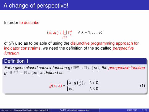
In order to describe

(x ,zk) ∈ ⋃j∈J

Γkj ∀ k = 1, . . . ,K

of (P1), so as to be able of using the disjunctive programming approach forindicator constraints, we need the definition of the so-called perspectivefunction.

Definition 1For a given closed convex function g ∶ Rm → R ∪ ∞, the perspective functiong ∶ Rm+1 → R ∪ ∞ is defined as

g(x , λ) =⎧⎪⎪⎨⎪⎪⎩

λ ⋅ g ( xλ) , λ > 0,

∞, λ ≤ 0.(1)


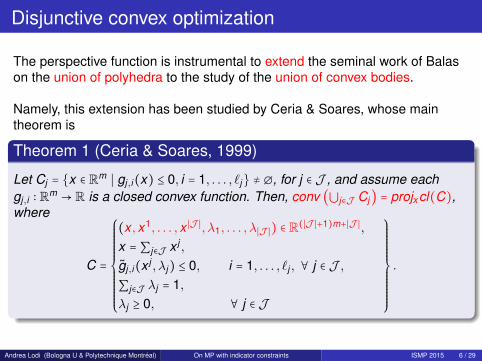
Disjunctive convex optimization

The perspective function is instrumental to extend the seminal work of Balason the union of polyhedra to the study of the union of convex bodies.

Namely, this extension has been studied by Ceria & Soares, whose maintheorem is

Theorem 1 (Ceria & Soares, 1999)

Let Cj = x ∈ Rm ∣ gj,i(x) ≤ 0, i = 1, . . . , `j ≠ ∅, for j ∈ J , and assume eachgj,i ∶ Rm → R is a closed convex function. Then, conv (⋃j∈J Cj) = projxcl(C),where

C =

⎧⎪⎪⎪⎪⎪⎪⎪⎪⎪⎪⎨⎪⎪⎪⎪⎪⎪⎪⎪⎪⎪⎩

(x ,x1, . . . ,x ∣J ∣, λ1, . . . , λ∣J ∣) ∈ R(∣J ∣+1)m+∣J ∣,x = ∑j∈J x j ,

gj,i(x j , λj) ≤ 0, i = 1, . . . , `j , ∀ j ∈ J ,∑j∈J λj = 1,λj ≥ 0, ∀ j ∈ J

⎫⎪⎪⎪⎪⎪⎪⎪⎪⎪⎪⎬⎪⎪⎪⎪⎪⎪⎪⎪⎪⎪⎭

.


Disjunctive convex optimization (cont.d)

The construction of Theorem 1 begins in a straightforward manner by creatingcopies x j of the initial variable x , each one constrained to lie in one of thedisjunctive sets Cj .

Then, the original x is a convex combination of these copies with weights λj .

In this way, the resulting bilinear terms λjx j lead to a set description of theconvex hull that is, however, nonconvex.

A simple transformation is then used to obtain the convex set C containing theperspective function.

Although now the weakness of the continuous relaxation of the bigMapproach seems solved by the strength of taking the convex hull in Theorem1, Ceria & Soares result leaves a couple of highly nontrivial computationalissues on the table.


Disjunctive convex optimization: computational issues

First, the closure of the perspective function has no algebraic representationin general.

In other words, the perspective function becomes non-differentiable for λj → 0.

The resulting numerical difficulties were already noticed in the process ofdesigning a branch-and-cut algorithm for general 0–1 mixed convexprogramming problems, based on lift-and-project cuts separated through analternative version of Theorem 1. [Stubbs & Mehrotra (1999)]

It is worth noting that for more than ten years there was no significantprogress in the separation of lift-and-project cuts for general mixed-integerconvex programming problems.

Recently, two major steps have been made to circumvent non-differentiabilityalgorithmically through the solution of “some” (potentially many) easieroptimization problems.

[Bonami (2011) and Kılınc, Linderoth & Luedtke (2011)]


Issue #2: Lifting up and projecting down again

The second difficulty associated with the practical use of Theorem 1 is the factthat the initial system is lifted into a space with a multiple dimension, i.e., C isdefined in R(∣J ∣+1)m+∣J ∣, which makes the optimization over it computationallychallenging.

Although the representation of the convex hull is theoretically compact in thenumber of variables, on the practical side the size of the resulting NLPs had asignificant impact on limiting the use of this disjunctive representation both

in the separation of L&P cuts for convex MINLPs and, in general,for formulating MP problems with indicator constraints.

However, in the context of indicator constraints, projecting out additionalvariables is possible in several special cases, as we will show in the following.

(It is worth noting that working on the original space of variables had a hugeimpact also on L&P cuts in the linear case.)

[Balas & Perregaard (2002) and Bonami (2012)]


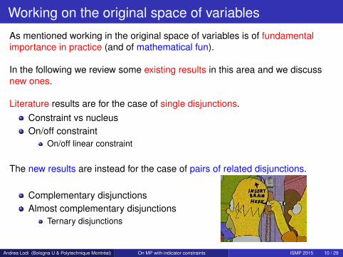
Working on the original space of variables

As mentioned working in the original space of variables is of fundamentalimportance in practice (and of mathematical fun).

In the following we review some existing results in this area and we discussnew ones.

Literature results are for the case of single disjunctions.Constraint vs nucleusOn/off constraint

On/off linear constraint

The new results are instead for the case of pairs of related disjunctions.

Complementary disjunctionsAlmost complementary disjunctions

Ternary disjunctions


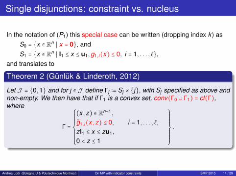
Single disjunctions: constraint vs. nucleus

In the notation of (P1) this special case can be written (dropping index k ) asS0 = x ∈ Rn ∣ x = 0, andS1 = x ∈ Rn ∣ l1 ≤ x ≤ u1,g1,i(x) ≤ 0, i = 1, . . . , `,

and translates to

Theorem 2 (Gunluk & Linderoth, 2012)

Let J = 0,1 and for j ∈ J define Γj ∶= Sj × j, with Sj specified as above andnon-empty. We then have that if Γ1 is a convex set, conv(Γ0 ∪ Γ1) = cl(Γ),where

Γ =

⎧⎪⎪⎪⎪⎪⎪⎪⎨⎪⎪⎪⎪⎪⎪⎪⎩

(x ,z) ∈ Rn+1,

g1,i(x ,z) ≤ 0, i = 1, . . . , `,zl1 ≤ x ≤ zu1,

0 < z ≤ 1

⎫⎪⎪⎪⎪⎪⎪⎪⎬⎪⎪⎪⎪⎪⎪⎪⎭

.


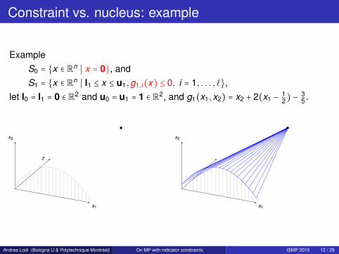
Constraint vs. nucleus: example

ExampleS0 = x ∈ Rn ∣ x = 0, andS1 = x ∈ Rn ∣ l1 ≤ x ≤ u1,g1,i(x) ≤ 0, i = 1, . . . , `,

let l0 = l1 = 0 ∈ R2 and u0 = u1 = 1 ∈ R2, and g1(x1,x2) = x2 + 2(x1 − 12) −

35 .

x1

z

x2

x1

x2


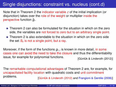
Single disjunctions: constraint vs. nucleus (cont.d)

Note that in Theorem 2 the indicator variable z of the initial implication (ordisjunction) takes over the role of the weight or multiplier inside theperspective function gi .

Theorem 2 can also be formulated for the situation in which on the zeroside, the variables are not forced to zero but to an arbitrary single point.Theorem 2 is also extendable to the situation in which on the zero sidethe set S0 is not a single point, but a ray.

Moreover, if the form of the functions g1,i is known in more detail, in somecases one can avoid the need to take the closure and thus the differentiabilityissue, for example for polynomial functions. [Gunluk & Linderoth (2012)]

The remarkable computational advantages of Theorem 2 are, for example, foruncapacitated facility location with quadratic costs and unit commitmentproblems. [Gunluk & Linderoth (2012) and Frangioni & Gentile (2006)]


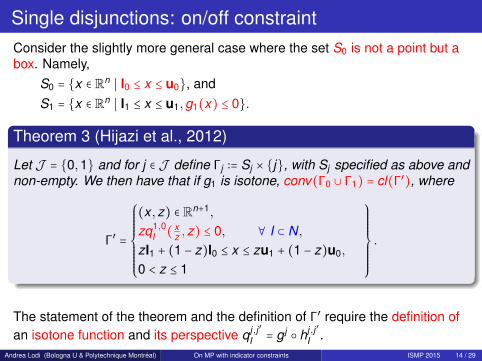
Single disjunctions: on/off constraintConsider the slightly more general case where the set S0 is not a point but abox. Namely,

S0 = x ∈ Rn ∣ l0 ≤ x ≤ u0, andS1 = x ∈ Rn ∣ l1 ≤ x ≤ u1,g1(x) ≤ 0.

Theorem 3 (Hijazi et al., 2012)

Let J = 0,1 and for j ∈ J define Γj ∶= Sj × j, with Sj specified as above andnon-empty. We then have that if g1 is isotone, conv(Γ0 ∪ Γ1) = cl(Γ′), where

Γ′ =

⎧⎪⎪⎪⎪⎪⎪⎪⎨⎪⎪⎪⎪⎪⎪⎪⎩

(x ,z) ∈ Rn+1,

zq1,0I ( x

z ,z) ≤ 0, ∀ I ⊂ N,zl1 + (1 − z)l0 ≤ x ≤ zu1 + (1 − z)u0,

0 < z ≤ 1

⎫⎪⎪⎪⎪⎪⎪⎪⎬⎪⎪⎪⎪⎪⎪⎪⎭

.

The statement of the theorem and the definition of Γ′ require the definition ofan isotone function and its perspective q j,j ′

I = g j hj,j ′

I .Andrea Lodi (Bologna U & Polytechnique Montreal) On MP with indicator constraints ISMP 2015 14 / 29

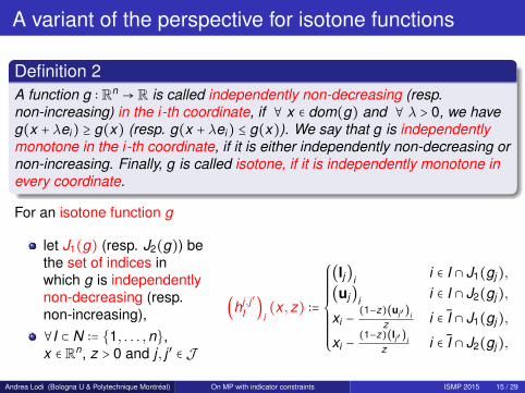
A variant of the perspective for isotone functions

Definition 2A function g ∶ Rn → R is called independently non-decreasing (resp.non-increasing) in the i-th coordinate, if ∀ x ∈ dom(g) and ∀ λ > 0, we haveg(x + λei) ≥ g(x) (resp. g(x + λei) ≤ g(x)). We say that g is independentlymonotone in the i-th coordinate, if it is either independently non-decreasing ornon-increasing. Finally, g is called isotone, if it is independently monotone inevery coordinate.

For an isotone function g

let J1(g) (resp. J2(g)) bethe set of indices inwhich g is independentlynon-decreasing (resp.non-increasing),∀I ⊂ N ∶= 1, . . . ,n,x ∈ Rn, z > 0 and j , j ′ ∈ J

(hj,j ′

I )i(x ,z) ∶=

⎧⎪⎪⎪⎪⎪⎪⎪⎪⎨⎪⎪⎪⎪⎪⎪⎪⎪⎩

(lj)i i ∈ I ∩ J1(gj),(uj)i i ∈ I ∩ J2(gj),

xi −(1−z)(uj′)i

z i ∈ I ∩ J1(gj),

xi −(1−z)(lj′)i

z i ∈ I ∩ J2(gj),


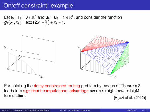
On/off constraint: example

Let l0 = l1 = 0 ∈ R2 and u0 = u1 = 1 ∈ R2, and consider the functiong0(x1,x2) = exp (2x1 − 9

5) + x2 − 1.

x1

z

x2

x1

x2

Formulating the delay-constrained routing problem by means of Theorem 3leads to a significant computational advantage over a straightforward bigMformulation. [Hijazi et al. (2012)]


Theorem 3 vs Theorem 1: Trade-off

On the one side, the advantage of Theorem 3 is the fact that we project backonto the original space of variables.

In fact, we can express conv(Γ0 ∪ Γ1) = cl(Γ′) as a subset of a(n + 1)-dimensional space. A direct application of Theorem 1 would lead toexpressing the convex hull as the projection of a subset of a(3n + 5)-dimensional space.

On the other side, this gain does not come for free. In Theorem 3, we needexponentially many constraints.

In particular, including all the simple bound constraints, we have 2n + 2n + 2constraints opposed to 4n + 9 that would result from a direct application ofTheorem 1.

In essence, an upper bound on the number of constraints needed to describethe convex hull is always exponential, although only in the number ofvariables involved in the constraint.


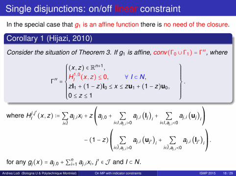
Single disjunctions: on/off linear constraint

In the special case that g1 is an affine function there is no need of the closure.

Corollary 1 (Hijazi, 2010)

Consider the situation of Theorem 3. If g1 is affine, conv(Γ0 ∪ Γ1) = Γ′′, where

Γ′′ =

⎧⎪⎪⎪⎪⎪⎪⎪⎨⎪⎪⎪⎪⎪⎪⎪⎩

(x ,z) ∈ Rn+1,

H1,0I (x ,z) ≤ 0, ∀ I ⊂ N,

zl1 + (1 − z)l0 ≤ x ≤ zu1 + (1 − z)u0,

0 ≤ z ≤ 1

⎫⎪⎪⎪⎪⎪⎪⎪⎬⎪⎪⎪⎪⎪⎪⎪⎭

.

where H j,j ′

I (x ,z) ∶=∑i ∈I

aj,ixi + z⎛⎝

aj,0 + ∑i∈I,aj,i>0

aj,i (lj)i + ∑i∈I,aj,i<0

aj,i (uj)i

⎞⎠

− (1 − z)⎛⎜⎝∑

i ∈I,aj,i>0

aj,i (uj ′)i + ∑i ∈I,aj,i<0

aj,i (lj ′)i

⎞⎟⎠.

for any gj(x) = aj,0 +∑ni=1 aj,ixi , j ′ ∈ J and I ⊂ N.


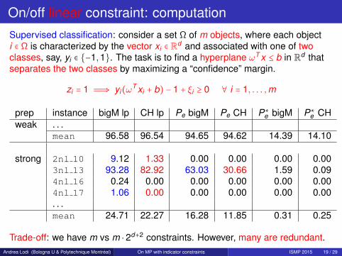
On/off linear constraint: computationSupervised classification: consider a set Ω of m objects, where each objecti ∈ Ω is characterized by the vector xi ∈ Rd and associated with one of twoclasses, say, yi ∈ −1,1. The task is to find a hyperplane ωT x ≤ b in Rd thatseparates the two classes by maximizing a “confidence” margin.

zi = 1 Ô⇒ yi(ωT xi + b) − 1 + ξi ≥ 0 ∀ i = 1, . . . ,m

prep instance bigM lp CH lp Pe bigM Pe CH P∗e bigM P∗

e CHweak . . .

mean 96.58 96.54 94.65 94.62 14.39 14.10

strong 2nl 10 9.12 1.33 0.00 0.00 0.00 0.003nl 13 93.28 82.92 63.03 30.66 1.59 0.094nl 16 0.24 0.00 0.00 0.00 0.00 0.004nl 17 1.06 0.00 0.00 0.00 0.00 0.00. . .mean 24.71 22.27 16.28 11.85 0.31 0.25

Trade-off: we have m vs m ⋅ 2d+2 constraints. However, many are redundant.Andrea Lodi (Bologna U & Polytechnique Montreal) On MP with indicator constraints ISMP 2015 19 / 29

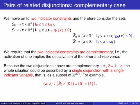
Pairs of related disjunctions: complementary case

We move on to two indicator constraints and therefore consider the setsS0 = x ∈ Rn ∣ l0 ≤ x ≤ u0,S1 = x ∈ Rn ∣ l1 ≤ x ≤ u1,g1(x) ≤ 0,

S0 = x ∈ Rn ∣ l0 ≤ x ≤ u0,g0(x) ≤ 0,S1 = x ∈ Rn ∣ l1 ≤ x ≤ u1.

We require that the two indicator constraints are complementary, i.e., theactivation of one implies the deactivation of the other and vice versa.

Because the two disjunctions above are complementary, i.e., z = 1 − z, thewhole situation could be described by a single disjunction with a singleindicator variable, that is, as a subset of Rn+1. For example,

(x ,z) ∈ (S0 × 0) ∪ (S1 × 1) .


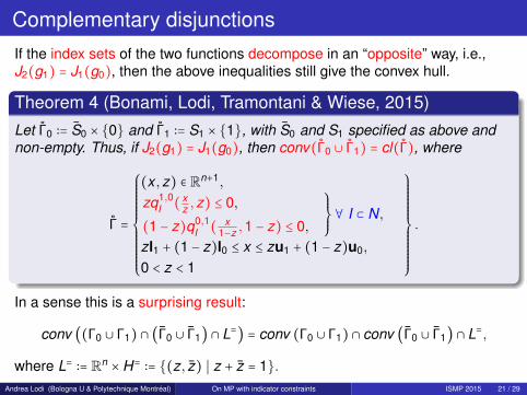
Complementary disjunctionsIf the index sets of the two functions decompose in an “opposite” way, i.e.,J2(g1) = J1(g0), then the above inequalities still give the convex hull.

Theorem 4 (Bonami, Lodi, Tramontani & Wiese, 2015)Let Γ0 ∶= S0 × 0 and Γ1 ∶= S1 × 1, with S0 and S1 specified as above andnon-empty. Thus, if J2(g1) = J1(g0), then conv(Γ0 ∪ Γ1) = cl(Γ), where

Γ =

⎧⎪⎪⎪⎪⎪⎪⎪⎪⎪⎪⎨⎪⎪⎪⎪⎪⎪⎪⎪⎪⎪⎩

(x ,z) ∈ Rn+1,

zq1,0I ( x

z ,z) ≤ 0,

(1 − z)q0,1I ( x

1−z ,1 − z) ≤ 0,

⎫⎪⎪⎬⎪⎪⎭∀ I ⊂ N,

zl1 + (1 − z)l0 ≤ x ≤ zu1 + (1 − z)u0,

0 < z < 1

⎫⎪⎪⎪⎪⎪⎪⎪⎪⎪⎪⎬⎪⎪⎪⎪⎪⎪⎪⎪⎪⎪⎭

.

In a sense this is a surprising result:

conv ((Γ0 ∪ Γ1) ∩ (Γ0 ∪ Γ1) ∩ L=) = conv (Γ0 ∪ Γ1) ∩ conv (Γ0 ∪ Γ1) ∩ L=,

where L= ∶= Rn ×H= ∶= (z, z) ∣ z + z = 1.Andrea Lodi (Bologna U & Polytechnique Montreal) On MP with indicator constraints ISMP 2015 21 / 29

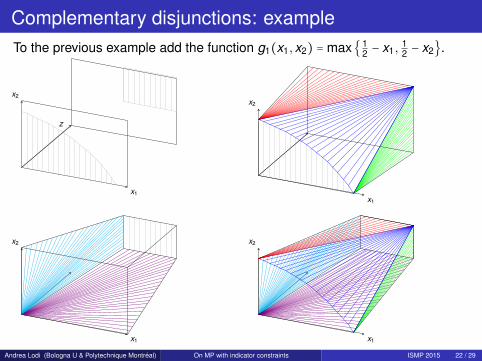
Complementary disjunctions: exampleTo the previous example add the function g1(x1,x2) = max 1

2 − x1,12 − x2.

x1

z

x2

x1

x2

x1

x2

x1

x2


Is J2(g1) = J1(g0) needed? Counterexample

Let l0 = l1 = 0 and u0 = u1 = 1, H0(x) = x − 12 and H1(x) = x − 3

4 , both of whichare non-decreasing in their first and only coordinate.

z

x

12

z

x

34

z

x

Open question: How to compute the convex hull in this case?


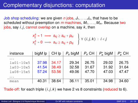
Complementary disjunctions: computation

Job shop scheduling: we are given n jobs, J1, . . . ,Jn, that have to bescheduled without preemption on m machines, M1, . . . ,Mm. Because twojobs, say i , j , cannot overlap on a machine, say k , then

xkij = 1 Ô⇒ skj ≥ ski + pki

xkij = 0 Ô⇒ ski ≥ skj + pkj

⎫⎪⎪⎬⎪⎪⎭∀ (i , j ,k) ∶ i < j

instance bigM lp CH lp Pe bigM Pe CH P∗e bigM P∗

e CH. . .la01-10x5 37.98 34.17 29.34 26.75 29.02 26.75la03-10x5 41.54 38.49 32.58 31.67 31.92 31.64la08-15x5 57.24 53.56 49.06 47.70 47.03 47.47. . .mean 40.31 38.64 36.11 35.01 34.98 34.60

Trade-off: for each triple (i , j ,k) we have 2 vs 8 constraints (reduced to 6).


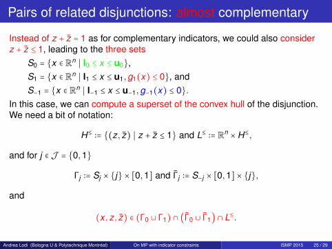
Pairs of related disjunctions: almost complementary

Instead of z + z = 1 as for complementary indicators, we could also considerz + z ≤ 1, leading to the three sets

S0 = x ∈ Rn ∣ l0 ≤ x ≤ u0,S1 = x ∈ Rn ∣ l1 ≤ x ≤ u1,g1(x) ≤ 0, andS−1 = x ∈ Rn ∣ l−1 ≤ x ≤ u−1,g−1(x) ≤ 0.

In this case, we can compute a superset of the convex hull of the disjunction.We need a bit of notation:

H≤ ∶= (z, z) ∣ z + z ≤ 1 and L≤ ∶= Rn ×H≤,

and for j ∈ J = 0,1

Γj ∶= Sj × j × [0,1] and Γj ∶= S−j × [0,1] × j,

and

(x ,z, z) ∈ (Γ0 ∪ Γ1) ∩ (Γ0 ∪ Γ1) ∩ L≤.


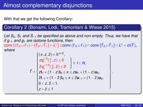
Almost complementary disjunctions

With that we get the following Corollary:

Corollary 2 (Bonami, Lodi, Tramontani & Wiese 2015)

Let S0, S1 and S−1 be specified as above and non-empty. Thus, we have thatif g−1 and g1 are isotone functions, thenconv ((Γ0 ∪ Γ1) ∩ (Γ0 ∪ Γ1) ∩ L≤) ⊆conv (Γ0 ∪ Γ1) ∩ conv (Γ0 ∪ Γ1) ∩ L≤ = cl(Γ),where

Γ =

⎧⎪⎪⎪⎪⎪⎪⎪⎪⎪⎪⎪⎪⎪⎪⎪⎪⎨⎪⎪⎪⎪⎪⎪⎪⎪⎪⎪⎪⎪⎪⎪⎪⎪⎩

(x ,z, z) ∈ Rn+2,

zq1,0I ( x

z ,z) ≤ 0

zq−1,0I ( x

z , z) ≤ 0

⎫⎪⎪⎬⎪⎪⎭∀ I ⊂ N,

zl1 + (1 − z)l0 ≤ x ≤ zu1 + (1 − z)u0,

zl−1 + (1 − z)l0 ≤ x ≤ zu−1 + (1 − z)u0,

0 < z, z < 1,z + z ≤ 1

⎫⎪⎪⎪⎪⎪⎪⎪⎪⎪⎪⎪⎪⎪⎬⎪⎪⎪⎪⎪⎪⎪⎪⎪⎪⎪⎪⎪⎭

.


Ternary disjunctions

Almost complementary disjunctions could also be modeled by a singleindicator variable assuming the values −1,0,1, i.e., ternary disjunctions.

Natural questions are1 is it possible to write the counterpart of Theorem 3 for this case?2 which is the relationship between these two ways of representing

essentially the same disjunction?

Question 1 has a positive answer but only in the special case of affinefunctions because we are unable to define the perspective function fornegative values of z.(The convexity-preserving property is otherwise lost.)

The answer to Question 2 is also somehow surprising.We can show that, at least for affine functions, the convex hull of the almostcomplementary disjunction is contained in the convex hull of the ternarydisjunction (when transforming everything into a common space).


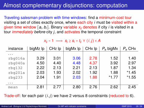
Almost complementary disjunctions: computation

Traveling salesman problem with time windows: find a minimum-cost tourvisiting a set of cities exactly once, where each city i must be visited within agiven time window [ai ,bi]. Binary variable xij denotes if city i is visited in atour immediately before city j , and activates the temporal constraint

xij = 1 Ô⇒ sj ≥ si + tij ∀ (i , j) ∈ A

instance bigMz lp CHz lp bigMx lp CHx lp Pe bigMx Pe CHx. . .rbg016a 3.29 3.01 3.06 2.78 1.52 1.40rbg040a 4.50 4.40 4.48 4.37 3.92 2.97rbg132 2.22 2.13 2.21 2.13 1.87 1.34rbg201a 2.03 1.93 2.02 1.92 1.88 *1.45rbg233 2.04 1.91 2.03 1.88 *1.77 *1.55. . .mean 2.81 2.77 2.80 2.76 2.62 2.45

Trade-off: for each pair (i , j) we have 2 versus 8 constraints (reduced to 6).


Computational facts, hopes and conclusions

The computation is mildly promising although not conclusive because there isno instance that the general-purpose solver IBM-ILOG CPLEX can solve withthe perspective formulation and cannot with the bigM one.

However, by taking a closer look at the inequalities in the previous slides onerealizes that, in the linear case, they have the structure of bigM constraints,and, in any case, they depend on the bounds on the involved variables.

This opens the possibility of extensively using bound tightening in the nodesof the branch-and-bound tree where the perspective constraints can bereplaced by locally-valid strengthened versions.

This is what has been proposed to effectively solve supervised classificationmodels and is now part of IBM-ILOG CPLEX algorithmic arsenal.

[Belotti et al. (2014) and IBM-ILOG CPLEX (v. 12.6.1)]

We believe/hope that combining disjunctive formulations with aggressive cutgeneration and bound reductions within the tree could lead to effectivealgorithms for hard MINLPs.


On mathematical programming with indicator constraints · On mathematical programming with...

Documents

Transcript of On mathematical programming with indicator constraints · On mathematical programming with...