On mathematical modelling of the self-heating of ...

Copyright is owned by the Author of the thesis. Permission is given for a copy to be downloaded by an individual for the purpose of research and private study only. The thesis may not be reproduced elsewhere without the permission of the Author.

ON MATHEMATICAL MODELLING OF THE SELF-HEATING

OF CELLULOSIC MATERIALS

A thesis presented in p arti al fulfilment of the requirements for the

degree of Doctor of Phi losophy in M athem atics

Robert Antony Sisson

June 1991

at M assey Unive rsity, New Ze al and

Massey University Library Thesis Copyright Form

Title of thesis: 0 r1 Mcd-�eM.a H c� l V1A ode 11 �� o.{: l;J..e se q:: -h et�t·h� op ce) I t.-1l o�' c rt1td-eV',·Ci lr

(1) (a) I give permission for my thesis to be made available to

readers in Massey University Library under conditions

determined by the Librarian.

(b) I . not ffish �thesis to be �e availabl�reades,s. 1thout my�itten consentAbr . . . mo. r'

,2) (a) I agree that my thesis, or a copy, may be sent to

another institution under conditions determined by the

Librarian.

(b) I do� wish my th�, or a copy, t<ybe sent to

a��er instituti_9JY'Without my w.;:.itfen conse� months.

(3) (a) I agree that my thesis may be copied for Library use.

(b) �not wi� thesis t�copied fgyr:ibrary us� ... months.

Signed ��Jt Date \'3. J LV\€ )£::\ l'1 \

The copyright of this thesis belongs to the author. Readers must

sign their name in the space below to show that they recognise

this. They are asked to add their permanent address.

NAME AND ADDRESS

Ro8e121 s 1 Ss oi\J 2.13 fb 12 b A-'Dw A-'/ A \Jt;tJ V E:: PAL-lV\ft2<;rON AJaf2:rl\-15

MASSEY UNIVERSil' LIBRARY

DATE I ' '""\. q I � Ju.ne \ q

ABSTRACT

This thesis consi ders mathemati cal mo delling of self-heating of cellulosi c materials,

and in parti cular the effe cts of moisture on the heating chara cteristi cs. Following an

introdu ctory chapter containing a literature review, Chapter 2 presents some

preliminary results an d an in dustrial case study. The case study, whi ch dis cusses a

' dry' body self-heating on a hot su rfa ce, investigates the following questions : (i)

how hot can the surfa ce get before ignition is likely? (ii) how well does the (slab

like) bo dy approximate to an infinite slab? an d (iii) how vali d i s the Frank

Kamenetskii approximation for the sour ce term? It is shown that the min imal stea dy

state temperatu re profile is stable when the temperature of the hot surfa ce is below a

certain criti cal value, an d boun ds for the higher stea dy state profil e are deriv ed.

Chapter 3 presents the thermo dynami c derivation of a rea ction- dif fusion mo del for

the self-heating of a moist cellulosi c bo dy, in clu ding the effe cts of dire ct chemi cal

oxi dation as well as those of a further exothermi c hy drolysi s rea ction an d the

evaporation an d con densation of water. The mo del contains three main variables: the

temperature of the bo dy, the liqui d water con centration in the bo dy, an d the water

vapour con centration in the bo dy. Chapter 4 investigates the limiting case of the

mo del equations as the thermal con du ctivity an d diffusivity of the bo dy be come

l arge. I n parti cular it is shown that, in this l imiting case, the mo del can have at least

twenty-five distin ct bifur cation diagrams, compare d with only two for the well

known mo del without the effe cts of moisture content. In Chapter 5 the maximum

p rin ciple an d the methods of upper an d lower solutions are use d to derive existen ce,

uniqueness an d mul tipli ci ty results for the stea dy sta te solutions of the spa tially

distribute d mo del. Finally, in Chapter 6, existen ce an d uniqueness results for the

time depen dent spatial ly distribute d mo del are derive d.

I would like to express my gratitude to my supervisors Professor Graeme

Wake and Mr Adrian Swift for their unfailin g help and enthusiasm throughout

my work. Thanks also to Or Alex McNabb and Mr Aroon Parshotam for

many helpful comments, Mr Richard Rayner for his help in producing the

graphics, Miss Fiona Davies for her typing of this thesis, Joanne for her

constant support, and Patricia for her friendship.

CHAPTER 1

1 . 1

1 .2

1 . 3

CHAPTER 2

2. 1

2.2

CHAPTER 3

3 . 1

3.2

3 . 3

3 .4

3.5

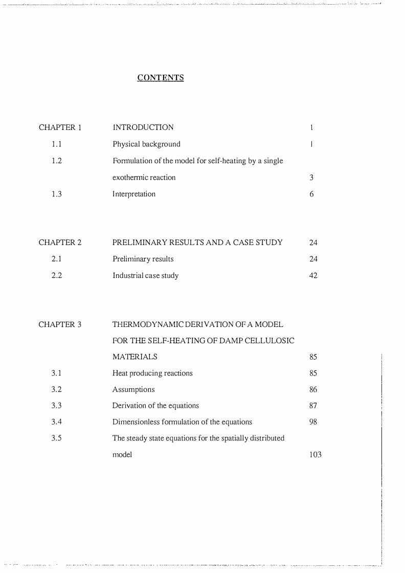
CONTENTS

INTRODUCTION

Physical background

Fommlation of the model for self-heating by a single

exothe nnic reaction

I nterpretation

PRELIMINARY RESULTS AND A CASE STUDY

Preliminary results

Industrial case study

T HERMODYNAMIC DER IVAT ION O F A MODEL

FOR T HE SELF- HEATING OF DAMP CELLULOSIC

MA TERIALS

Heat producing reactions

Assumptions

Derivation of the equations

Dimensionless formulation of the equations

The steady state equations for the spatially distributed

model

3

6

24

24

42

85

85

86

87

98

1 03

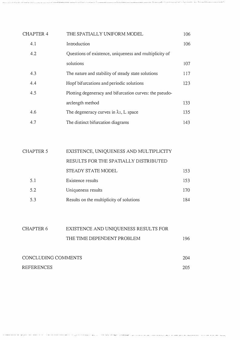
CH APTER 4

4. 1

4.2

4.3

4.4

4 .5

4 .6

4. 7

CHAPTER 5

5 . 1

5 .2

5 .3

CHAPTER 6

T HE SPATIALLY UN IFORM MODEL

Introduction

Questions of existence, uniqueness and multiplicity of

solutions

The nature and stability of steady state solutions

Hopf bifurcations and periodic solutions

Plotting degeneracy and bifurcation curves : the pseudo-

arclength method

The degeneracy curves in AI, L space

The distinct bifurcation diagrams

EXISTENCE, UNIQUENESS AND MULTIPLICITY

RESULTS FOR T HE SPATIALLY DISTRIBUTED

STEADY STATE MODEL

Existence results

Uniqueness results

Results on the multiplicity of solutions

EXISTENCE AND UNIQUENESS RESULTS FOR

THE TIME DEPE NDENT PROBLEM

CONCL UDING COMMENTS

REFERENCES

1 06

1 06

1 0 7

1 1 7

123

1 33

135

143

153

153

1 70

1 84

1 96

204

205

1

CHAPTER 1

Introduction

1.1 Physical background

A body is said to be 'self-heating' when i ts temperature rises due to a process occurring

i nside the body i tself. Under certain conditions this temperature rise may be sufficiently

l arge so as to i nduce the body to thermally ignite. 'Spontaneous ignition' or 'spontaneous

combustion' has then occurred.

Fires due to spontaneous combustion arising in practice can general ly be placed into one

of two categories, the common denominator being an internal exothermic process. The

first category is where a ' smal l' body of material such as a sack , small pi le or dust layer is

stored subject to high ambient conditions (for example on a hot surface) and/or at a high

initial temperature (for example chemical s from a drying process) . Generally these fires

are induced over quite a smal l time scale, sometimes a matter of hours or days . Typical

scenarios for fires occurring in this category would include: the last batch of laundry from

an i ndustrial cleaning process catching fire in the early hours of the morning, or forest

l i t ter, for example gum leaves, igniting due to the proximity of a barbecue fire, or a

woodchip/oil dust layer igniting on a hot fibreboard press . The second category is

associated with fires that occur over far longer time scales, sometimes months , and at

lower ambient cond itions, sometimes room temperature - the spontaneous combustion of

l arge stockpiles of material . Typical materials would include hay, woodchips, wool and

bagasse (bagasse being the fibrous residue of the extraction of sugar from sugar cane) .

The economic importance of the study of spontaneous combustion can be p laced in

perspective by analysing the following table from Bowes li ] , whi ch summarizes statistics

of building fires in the United Kingdom between 1 970- 1 973 .

2

Ye!lr 1970 1971 rm 1973 1970 1971 1972 1973 Number or nre.s 9<14U !9310 100011 1ll532J

Suppo�d ou� Proportion o( :all .lirc:5 � lroporooa o( :all ru-es assi::ucd to to�= zj-rca =- which wen: also laJ"':e{3}

E!ectric::U appliances 28.5 29.5 29.8 31..2 0.53 0.51 0.48 0.54

and installations

p riroary fuel burning 0..39 0.31 0.46 appliances and 20.3 19.3 19.2 18.5 0..35

ins talla t.i 0 os (1 )

Childro p!ayin g with 8.5 9.1 9..9 9.5 0..14 0.34 0.31 0.36

.f1re, eg matches

S moker's rnate:ials 8.7 8.0 7.7 8.3 0.73 0.77 0.81 LOO Malicious or inten- 4.1 5..9 7.0 7..3 3.2 3..3 3.3 3.6 tional ignition

Spontaneous 0.61 0.55 OAT 0.41 1.8 2.9 3.2 2.5 combustion

Other known 15.9 14.6 14.4 13.5 0.65 0.67 0.67 0.85 C:l.USCS (2)

Unkno.,.,-o 13.4 13.0 11.7 11.0 4.5 5.5 6.2 6.1

(I) Solid fuel, oil, gas, LPG, acetylene

(2) Lis:e::l and unlisted, �-.:eluding rubbish burning and inclnding 'other and unspecified fu·es'. less than 5 per cent of total fi.res assigned to each

(3) Dir= loss in e.-.:cess of £10 000.

Figure 1.1 Building fire statistics 1 9 70- 19 73 .

These s tatistics indicate that spontaneous combustion i s second only behind 'malicious or

intentional damage' as the most common of the assigned causes of l arge fires .

In terms of the mathematical modelling of self-heating bodies, then, the three main areas

of interest, which of course are closely related, are:

( i ) Critical size. What is the ' largest' size of stockpile in which we can safely s tore a

given materia l a t a given ambient temperature and i nitial temperature ?

3

(i i ) Critica l ambient temperature. What is the hottest sto rage tempe rature we can

s afely apply to a given stockp ile at a gi ven initi al tempe ratu re?

( i i i ) Cri tica l init ia l tempera tur·e. To what tempe rature shoul d we al low a bo dy to cool

befo re sto ring it in a stockpile of given dimensions an d given ambient temperatu re?

The mathematical an alysis of most inci dences of fi res cause d by spont aneous combustion

can be re duce d to a consi de ra tion of one of the above th ree facto rs.

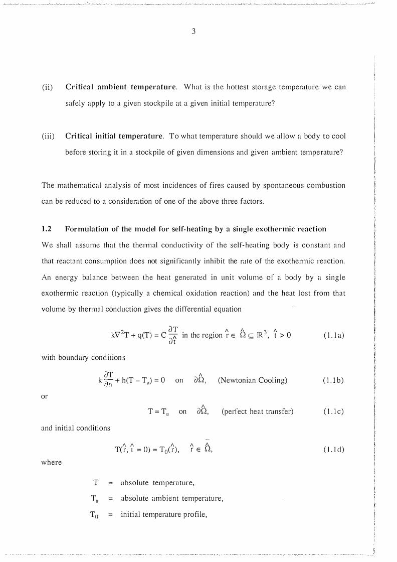
1.2 Fonnulation of the model for se l f-heating by a single exother·mic reaction

We shall assume th at the the rm al con ductivity of the self-he ating bo dy is constant an d

that reac tant consumpt ion does not signi fican tly inhibit the mte o f the exothe rmic re action.

An ene rgy bal ance between the he at gen erat ed in uni t volume o f a bo dy by a single

exothe rmic reac tion (typically a chemical oxi dation reaction) an d the heat lost f rom th at

volume by the rmal con duction gives the di ffe rential equation

2 aT 1\ 1\ 3 1\ k\7 T + q(T) = C ;:: in the region rE Q � JR·, t > 0

dt

with boun da ry con dit ion s

o r

()T 1\ k ::;--- + h(T - T .1) = 0 on ()Q, on '

1\ T = Ta on ()Q,

(Newtonian Cool ing)

(pe rfect he at t ransfe r)

an d initi al con ditions

whe re

T =

Ta =

T o =

1\ 1\ 1\ 1\ 1\ T( r, t = 0) = T 0( r) , rE Q,

absolute tempe rature,

absolute ambient tempe ratu re,

initial temperatu re p rofi le,

( 1 . 1 a)

( l. l b )

( l. lc)

( !. Id)

4

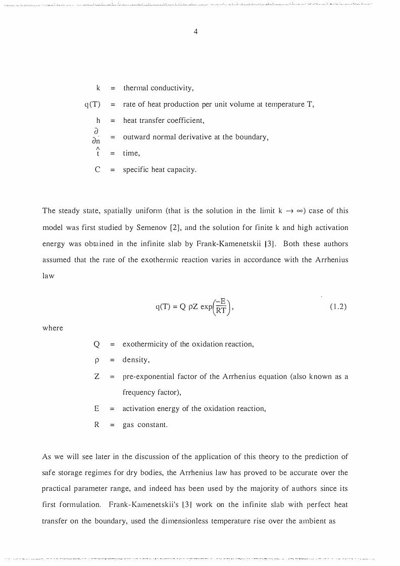
k = thermal conductivi ty,

q (T) = rate of heat production per unit volume at temperature T,

h = heat transfer coefficient, ()

outward normal derivative at the boundary, dn = 1\ t = t ime,

c = specific heat capacity.

The s teady s tate, s patially uniform (that is the solution in the limit k -7 oo) case of this

model was first studied by Semenov [2] , and the solution for fin i te k and high activation

energy was obtained in the infin i te s lab by Frank-Kamenetski i 13] . Both these au thors

assumed that the rate of the exothe nnic reaction varies in accordance with the Arrhen ius

law

where

q (T) = Q pZ exp(��) ,

Q = exothermicity of the oxidation reaction,

p = dens i ty ,

( 1.2)

Z = pre-exponential factor of the Arrhen ius equation (also known as a

frequency factor) ,

E = activation energy of the oxidation reaction,

R = gas constant.

As we will see later in the d iscussion of the appl ication of this theory to the prediction of

safe storage regi mes for dry bod ies, the A rrhenius l aw has proved to be accurate over the

practical parameter range, and indeed has been used by the majority of authors since i ts

first formulation. Frank- Kamenetsk i i ' s 1 3 1 work on the i n fin i te slab with perfect heat

transfer on the boundary, used the cl i mensionless temperature rise over the ambient as

5

so the steady state problem becomes, in dimensionless coordinates

with

where

8 = 0, at r = ± 1 ,

a0 = half-width of the body,

Ea =

8 =

r =

RTa E' 2 (-E) pQa0 E Z exp RT� 2 kRTa

dimensionless length ( = :0)

-1 <r< 1 ,

( 1 . 3 )

( 1 .4a)

( 1 .4b)

( 1 .4c)

The parameter 8 is often referred to as the Frank-Kamenetskii parameter. FrankE Kamenetskii observed that, provided RT >> 1 (i.e. Ea << 1 ) , and 8 is not too large, the a

problem reduces to the equation

with

d28 dr2 +8exp8 = 0, -l<r<l,

8 = 0, at r = ± 1 ,

which has the well-known closed form solu tion

8(r) = fnF - 2fn(cosh(r cosh-1�F) ) ,

( 1 . 5 a)

( l .Sb)

( 1 . 6a )

6

where F i s the solution of the transcendental equation

( 1 .6b)

The assumption £a << 1 is known as the Frank- Kamenetski i approximation, and is the

most commonly used , but not th e only such approximation , in the li terature. For example

Gray and Harper 1 4 1 in troduced a quadratic approx imation to th e Arrhen ius term i .e.

where b 1 = 1, b 2 = e-2, b3 = I.

( 1 . 7)

The merits and consequences of the Frank-Kamenetsk i i approx imation wil l be d iscussed

again in Chapter 2.

1.3 Interpretation

I t i s well-known ( the veri fication involves simple calculus) that for o < 0.88 two solutions

to ( 1 .6a, b) exist , th e lower of which is stable (i n a time sen s e) and the h igher of wh ich is

unstable. But for o > 0.88 no sol utions exist. Frank- Kamenetski i iden tified this transition

with the onset of thermal ign i tion, s ince for o > 0.88 no stable steady state profile wil l

exist and the temperature of the body will r ise in an unbounded manner with ti me. The

value o = 0.88 is referred to as ocrit for the infin i te s lab. This behaviour in the o, 1 1 8 1 10

space, where 118110 = max 18 (r) l , is summarised in Figure 1.2 below rE £1

7

11 e llu

Figure 1.2 Typical 8, 116110 bifurcation diagram for the infinite slab with the Frank-

Kamenetskii approximation.

For the infini te cylinder and unit sphere, 8crit = 2.00, 3 . 32 respectively. For more general

shapes (cubes, fini te cylinders etc.) Boddington, Gray and Harvey [5] have introduced the concept of a root-mean-square 'Frank-Kamenetskii' radius, r0, of a body, and it is this

approach that is used by experimentalists in laboratory scale tests.

Several variations of this basic model have been studied, both with and without the Frank-

Kamenetskii approximation. For example: a model with reactant consumption

(Boddington et al [6] ) , criticality with variable thermal conductivity (Wake [ 7] ) , ignition of

a self-heating body subject to asymmetric boundary conditions (Thomas and Bowes [8] ,

S houmann and Donaldson [9] and S isson, Swift and Wake [ 1 0] ) , and a model for an

exothermic reaction sustained by a single diffusing reactant (B urnell et al [ 1 1 ] ) . In 1 989

Burnell et at [ 1 2] presented a paper questioning the appropriateness of the classical

Frank-Kamenetskii formulation, particularly the use of the ambient temperature in the non-

8

dimensionali zation of the body temperature. They suggested an alternative formulation for

the non-dimensiona li zation of the system i .e.

This gives the dimensionless form of the parabolic sys tem (1. 1 a, b, c, d) , ( 1 .2) as

with

or

and

where

=

2 (-1 ) dll V u + 11 exp - = -ll d t '

r E .Q,

dll "\ + Bi (u - U) = 0, r E ().Q, on

(Newton ian cooling)

u = U , r E ().Q,

(perfect heat transfer)

u(r, t = 0) = u0(r) ,

pQZRa5 kE

t > 0,

( 1 . 8 a)

( 1 . 8 b)

( 1 .9a )

( 1 .9b)

( 1 .9c)

( 1 .9d)

= an appropriate characteri stic length such as the half-width of the

Bi =

=

r =

body, ha 0

dimen si onless B iot n umber = k, 1\ t k ? c , a o 1\ r

1\ 1\ and .Q, ().Q are the scaled representations of .Q, ().Q respectively .

9

The steady states of this system are given by

(I. 9e)

with the same boundary cond itions (1 .9b) or ( 1 .9c).

Their basic idea was that in most practical si tuations (and laboratory scale tests) Ta, the

ambient temperature, i s the most access ib le control parameter, and hence U (the dimension le s s representat ion of Ta) i s the natural bifurcation , or 'di s t i nguished' , parameter. In the Frank-Kamenetski i formulation Ta appears in 8, o and Ea, whereas i n the new formulat ion Ta appears only in U. As Burnell et al explain th is means that for a

bifurcation diagram in U, llull0 space, Ta, crit> the cri tical value of the ambient temperature, ( RTa crit) can be observed directly from the graph as Ucrit = E For the Frank-Kamenetski i

formulation, however, an iterative process must be used to find Ta. crit from the o, 118110 bifurcation diagram as fol lows:

RT ·

( 't ) • l 1 f' T I . l . a crll use a tna va ue o · a, crit w uc 1 gives Ea = E

( i i ) record ocrit from the o, 118110 plot;

(ii i ) from th is value of ocrit calculate the next approximation to Ta, crit·

RTa . A lso Since the r:ran k-Kamene t sk i i approx imation In effect sets Ea = · E - = 0, this

approximation is obviously inappropriate in the new formulation. In their 1 990 paper, Wake et al [ 1 31 presented exi stence, uni queness and mul ti p l ic i ty resul ts for the steady

states of the model using th i s new dimensionless formulation . For the analysis of the

model i n this thesis we wi l l use the new formulation of Burnel l et a! [ 1 2] and the ful l

10

Arrhenius representation of the heat balance equation, i .e . we will refrain from u sing the

Frank-Kamenetskii approximation .

In the chemical literature the most common approach in analysing safe storage regimes for

particul ar materi als is to invoke the Frank-Kamenetskii approx imation and the concept of

Frank-Kamenetskii radius and then extrapolate to resu lts for practical stockpi les from

those obtai ned from laboratory scale tests . Using the Frank-Kamenetski i approximation the heat balance equation ( 1.1 a), ( 1.2) for a system with one characteristic dimens ion (a0)

becomes

cJ2e i de -2 + "": -cl· + o(ao) expe = () dr I I ( 1. 1 0)

where j i s a shape factor and o is as given i n ( 1 .4c). Boclclington et al [5] give the shape

factor j and the cri tical value of the parameter o for non-standard shapes as

where

and

( 3r2 ) j = rt - 1 ,

3V rs = s '

ro = the root mean-square radius,

V = volume of the body,

s = smface area of the body,

ocrit = 3(2j+6) I U+ 7) .

( l . l l a)

( l . l l b)

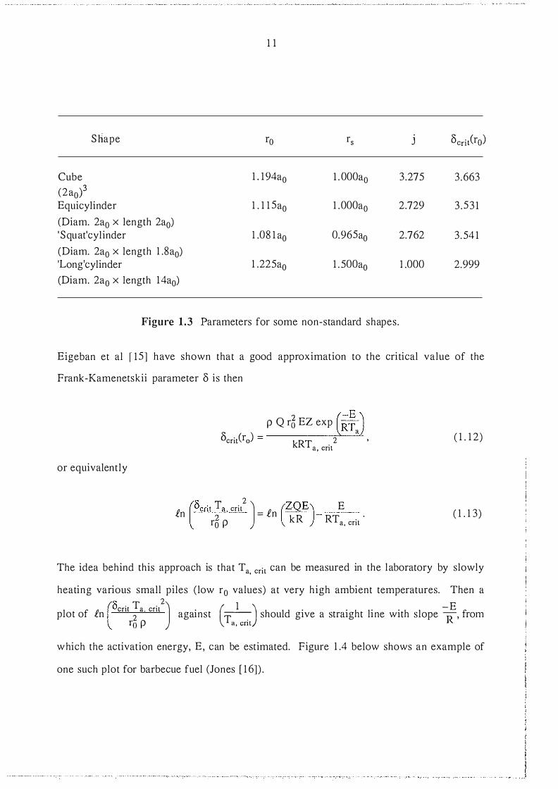
The values of r0, j and ocrit are given for various shapes, taken from Gray, Griffiths and

Hasko f 1 4 ] , in Figure 1.3 below.

1 1

Shape ro rs J c\ritCro) Cube 1. 194a0 1 . 000a0 3.275 3.663 (2ao)3 Equicylinder 1 . 1 1 5a0 1 .000a0 2.729 3.531 (Diam. 2a0 x length 2a0) 'Squat' cylinder 1 .081 a0 0.965a0 2.762 3. 541 (Diam. 2a0 x length 1 .8a0) 'Long' cylinder 1 .225a0 1 . 500a0 1 .000 2.999 (Diam. 2a0 x length 14a0)

Figure 1.3 Parameters for some non-standard shapes.

Eigeban et al r 15] have shown that a good approximation to the critical value of the Frank-Kamenetskii parameter o is then

or equivalently

p Q r6 EZ exp (r*.) OcritCro) = kRT . 2 • a, crll

in (Ocrit �a crit2 ) = in (ZQE)- E . r0 p kR RT a, crit

( 1 . 1 2)

( 1 . 1 3)

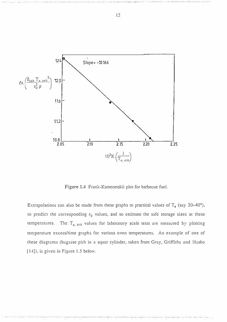
The idea behind this approach is that Ta, crit can be measured in the laboratory by slowly heating various small piles (low r0 values) at very high ambient temperatures. Then a (o . T . 2) ( 1 ) -E plot of in ern 2 a cnt against � should give a straight line with slope R' from ro p a, cnt

which the activation energy, E, can be estimated. Figure 1 .4 below shows an example of

one such plot for barbecue fuel (Jones [ 1 6] ) .

12

Slope= -10166

112

10.8 '---------�-------1-----1-_.::.... __ __. 2.05 2.10 2.15 2.2D 2.25

103K (-1-) Ta, crit

Figure 1.4 Frank-Kamenetskii plot for barbecue fuel.

Extrapolations can also be made from these graphs to practical values of Ta (say 20-40°), to predict the corresponding r0 values, and so estimate the safe storage sizes at these

temperatures. The Ta. crit values for laboratory scale tests are measured by plotting

temperature excess/time graphs for various oven temperatures. An example of one of

these diagrams (bagasse pith in a squat cylinder, taken from Gray, Griffiths and Hasko

ll4]), is given in Figure 1.5 below.

1-<J

2') 40

13

60

Time (min}

470·6

80 100

FigUI·e 1.5 Temperature excess/time graphs for bagasse pith in a squat cylinder,

for varying oven temperatures.

It can be seen from Figure 1.5 that there is a marked difference between the subcritical

and the supercrirical behaviour of the body. For oven temperatures above 470.8K, the

body temperature continu es to rise until (ultimately) ignition occurs. But for oven

temperatures below 470.6K the temperature excess achieves a maximum then falls as

reactant is consumed. Thus on the basis of this diagram, Ta. crit for this particular body is

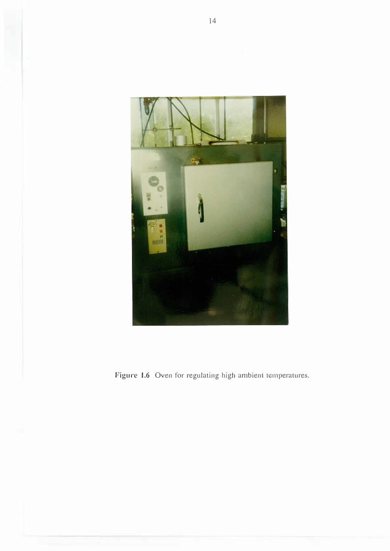
470.7K ± O.lK. Figures 1.6, 1.7 and 1.8 below show some typical apparatus used in these

laboratory scale tests (at the School of Chemistry, Macquarie University, Sydney,

Australia).

14

Figure 1.6 Oven for regulating high ambient temperatures.

15

Figure 1.7 Cylinder in oven.

16

Figure 1.8 Size range of vessels for laboratory scales tests.

1 7

This technique o f extrapolation from laboratory scale tes ts has been applied t o a wide

range of materials. Results from the literature are summarized in Figure 1 .9 below.

STORAGE CONDITIONS COMMENT ON MAT ERIAL ambient temperatures in oc REFERENCE

critical heights in metres MOISTURE FACTORS?

WOOL Amb. temp. 40 Jones ll7] YES Cril. height 6.6

QUEENSLAND Amb. temp. 40 20 Gray et al 114] YES BAGASSE Crit. height 66 276

HOPS Amb. temp. 40 J ones and Raj ll8] NO Cril. height 2.9

EUCALYPTUS Amb. temp. 40 25 Joncs and Raj ll9] NO L EAVES Cril. height 3.9 6.9

FIJIAN Amb. temp. 40 25 Raj and Jones 120] YES BAGASSE Crit. height 16.3 37.4

FIJIAN Amb. temp. 40 25 Raj and Jones 1201 YES HARDWOOD Crit. height 39 95 FLAKES

NSW WOOD Amb. temp. 40 25 Jones and Raj 1191 NO* SI-IAVING S Crit. height 48.5 126

NSW RICE Amb. temp. 40 25 Raj and Jones 1201 YES HUSKS Crit. height 25.5 63

CHEMICALLY Amb. temp. 40 30 B owes and Cameron YES ACTIVATED Crit. height 2.5 4.8 121] CARBON

Figure 1.9 Table of storage predictions from the l i terature.

* in effect this is a ' yes' s i nce Jones and Raj state that this result 'corresponds well with

the value for Queensland bagasse' .

In more than half of these references the authors acknowledge that the bounds on the safe

s torage heights obtai ned at real i s tic a mbient temperatures were someth ing of an

overestimation . For example Raj and Jones ! 20 ] state

1 8

"al l test materials show satisfactory conformity to the predictions of thermal

ignition theory when heated in baskets . . . When the results are extrapolated to

outdoor temperatures, all test materials gave surprisingly high values of the

calculated maximum stockpile height".

Gray, Griffiths and I -I asko [ 1 4] conjectured that thi s discrepancy is due to the effects of

moisture content in the real-sized stockpiles. I t appears to be a major fau lt in the process

outlined above that, s ince typical oven temperatures are above 1 00°C, after an init ial

period during which water evaporated from the system, the laboratory scale tests can only

measure the amoun t of heat produced by 'dry ' materials . Any data on the heat produced by

ancillary react ions associated with the presence of water in the body e.g . hydrolysis or

microbial factors, is bound to be lost. This is acknowledged by Jones [ 1 6]

" . . . however, as has been poin ted out more than once to the author, such

extrapolat ions may require caution . It may happen that processes are occurri ng in

the 'real' stockpile wh ich are absent from the laboratory test, for example moisture

effects and creation of reactive new surface by breakage on handling . I n such

circumstance the extrapolation would be of doubtful mean ing" .

This would also explain why the laboratory scale tests correspond so well to the Frank

Kamenetskii model (see Figure 1 .4) , which only accounts for heat produced by a dry

material . It is thought by many au thors , hence the comments on moisture content

mentioned in Figure 1 .9 , that it i s this underestimation of the amount of heat being

produced inside the self-heati ng stockpiles that is the cause of the overestimation of the

safe stockpiling sizes.

1 9

In a 1 973 paper Smith [22 ] summarised the causes of self- heating i n wet wood chips as

( i ) the metabolism of living wood parenchyma cells in fresh wood chips ;

(ii) the metabolism of bacteria and fungi ;

(iii) direct chemical oxidation ;

( iv) acid h ydrolysis of cel lulose.

We wil l assume these to be the mam heat producing components in all s toc kpiles of

cel lulosic materials. Fac tor (i) will only be present if the material in the s toc kpile has

been cut fairly recently . I t can also be ignored if, for example , the material h as gone

through an industrial refining process prior to stoc kpiling . Factors (ii) and (iv) can only

occur if there is moisture present in the body. We will loo k at the data for the production

of heat by the metabolism of bacteria and fungi in a particular material (bagasse) later in

this in troduction . Fac tor (iii) is the c lassical exothermic process of the Fran k

Kamenets kii model , which can occur whether or not moisture is present in the stoc kpile.

The effec ts of moisture on the chemical/physical processes occurring in stoc kpiled

cellulosic materials have been discussed by Gray , Griffiths and Hasko [14].

( i ) evaporation and loss of water can confer an endothermicity which tends to stabilise

the system ;

(ii) completely dry cellulosic materials are hygroscopic. The rate of heat release which

is due to condensation of water vapour and evolution of its laten t heat can be

sufficient to cause self-heating and thermal ignition ;

(iii) when movement of water t hrough a mass ta kes p lace by evaporation and

condensation, no net thermal effect will result when the two rates balance. The

overall heat release from the system will then approximate to t hat of dry material

at the same temperature ;

20

( iv ) balanced inte rnal rates of evaporation and condensation do not lead to identical

conditions for criticality of wet and dry masses. The ther mal diffusivity with i n wet

material is greater than that within dry material and the stabil i ty of the wet mass i s

enhanced because o f this ;

( v ) When a net loss o f water occurs from the system, there i s a gradual decrease in

thermal diffusivity ;

(v i ) as long as water rema ins 111 the system, l iqu id-phase oxidations and acid

hydrolysis of hemicel lu lose (an isomer of cel lu lose) may take place, making

add ition al contributions to the heat release rate.

I t is clear that , as well as taking into account the amount o f heat produced by the extra

exother mic re actions due to moisture content per se, any mathe matical model for 'self

heating with moisture content' must also i nclude the exother mic process of water v apour

condens ation, and the endothermic process of liquid water evaporation.

In the l ight of the obvious over estimation of safe storage regi mes for bagasse, as seen in

Figure 1 .9 , and in an attempt to gain further i nsight in to the reasons for th is discrepancy,

some experi mental work has recently been c arried out at the Sugar Research I nstit ute at

Mac kay, Queensland. Trials were conducted on various s tockpiles including identical

stockpiles with and without added H2S04 (the presence of H2S04 kills microbes in the

stockpile). The results were given in Dixon [23] and are summarised below .

( i ) the dry bagasse reaction alone is not sufficient to cause spontaneous combustion in

ful l size stockpi les ;

( i i ) microbiological h eat generation can be of little significance in i nitial bagasse

stockpi le temperature increases ;

2 1

(iii) there must exist one or more low temperat ure reactions which generate rapid initial

chemical heating in bagasse stockpi les ;

( iv ) preliminary micro-calorimetric investigations wi th bagasse a t low temperature

(60°C) show considerably enhanced heat generation in the presence of water ;

( v ) the rel ative importance of wet cellulose oxidation and a queous phase oxidation of

microbiological and hydrolysis by-products has not been established ;

( v i ) little change will occu r in the total moi sture content of the bulk of the bagasse

stockpile duri ng normal heating.

Work by Gray and Scott [24 1 showed that the initial bagasse storage temperature,

typical ly 50-70°C, would not be sufficient to i nduce thermal ign i tion in stockpi led dry

bagasse. G ray and Scott calculated that for dry bagasse an init ial temperature greater

than 90°C would be re quired for ignition in practical stockpile sizes and in the usual

ambient temperature range. In comparison with the dry model, very li ttle theoretical work

has been clone on the self-heat ing of clamp stockpiles.

In 1 939 Hen ry [25] published a paper on work arising from the analysis of the uptake of

moisture by cotton bales. He considered the diffusion of one substance through another in

the pores of a solid body which could absorb and immobi lise some of the diffusing

substance. Due to the smal l s ize of the pores encountered in these stockpiles and the fact

that many of them are fil led wi th li quid , Henry neglected the influence of convection in the

model. There was also no account made of the influence of heat production by oxidation or

hydrolysis reactions within the body . As Bowes [1 ] , page 296, states

"The transient diffusion of heat and moisture through porous hygroscopic materials

was considered theoretically by Henry with particular reference to temperature and

moisture changes in bales of textile fibres . . . He suggested that the analysis might

22

be extended to include s imultaneous heat generation by other processes but did not

pursue th is interesting poss ibility " .

In the 1 970's, Walker and eo-workers (e.g. Walker and Harr ison 1 26] , Walker and Jackson

[27 ] , Walker and Manssen [28] ) proceeded by essentially us ing the Frank-Kamenetskii

model , but by operat ing at lower oven temperatures (80-92°C), they were able to include

some of the effect of the moist ure content. This model had the fault that i t ' lumped' two,

essential ly dist inct, reactions in the same Arrhenius term. Also no account was made of

the evaporation or condensation of water . In 1 990, Gray and Wake [29] considered a

spatially uniform model, analys ing the effects of condensat ion/evaporat ion of water i n

con junct ion w ith th e e xotherm ic o xidat ion react ion. In the ir analys is Gray and Wake used

the quadrat ic a ppro ximat ion ( 1 .7) to the Arrhen ius term. How ever as they s tate in their

paper

11 we w ill assume that there are no e xtra self-heat ing reactions in the a queous

phase, although there undoubtedly are for some mater ials, such as bagasse" .

Finally, again in 1 990, Gray 1 30 1 presented a spat ially uniform model wh ich un if ied all the

main factors thought to be involved in the self-heating of mo ist cellulos ic stockpiles i.e.

( i) the heat prod uced by the o xidat ion react ion ;

( ii ) the heat produced by the hydrolys is react ion ;

(ii i) the en clothermic evaporat ion process ;

( i v ) the exotherm ic condensat ion process ;

( v ) the heat lost clue to Newtonian cool ing.

23

Gray also included a term to represent the water consumed by the hydrolysis reaction.

We have decided to ignore this term in our analysis. We do this for two reasons : (a) on

the grounds of consi stency, in that the model also 'neglects' the consumption of the other

two reactants i .e . cellu lose and oxygen, and (b) because steady state analysis with non

trivial concentrations of each species requires that all reactant consumption i s 'neglected'

(otherwise as t --7 oo the water content wil l tend to zero which contradicts observation

(vi) of Dixon [23] mentioned earlier) . 'Neglect of reactant consumption' in this con text

means that we will assume that the consumption of the reactants does not effect the rates

of any of the reactions in any way, i .e . there is always 'enough' of the reactants to fu lly

sustain all the reactions. This model was formulated in the wake of the Sugar Research

Insti tute 's comment on the minimal effects of microbes on the self-heating of bagasse.

How well the neglect of the heat produced by microbes can be justified for materials other

than bagasse is an open question to a certain extent . However it seems reasonable to

assume that , since all cel lu losic materia ls have basically very simi lar chemical

constituents , the heat produced by the hydr olysis reaction i s the dominant factor when

considering ancillary exothermic reactions due to moisture effects. It is the mathematical

analysis of this slight variant of Gray's model, and the corresponding spatially distributed

model , that we shall be main ly considering in this thesis .

Before embarking on this we wil l consider a case study involving self-heating by a single

exothermic reaction of a (dry) body on a hot surface. This example will i l lustrate the

power of s teady state ignition theory in practical circumstances and introduces some

further importan t concepts such as the maximum principle and the method of upper and

lower solu tions . We also in troduce some new results on the stability of the minimal

steady state solution, and on bounds for the higher steady state reached beyond criticality.

24

CHAPTER 2

Preliminary results and a Case Study

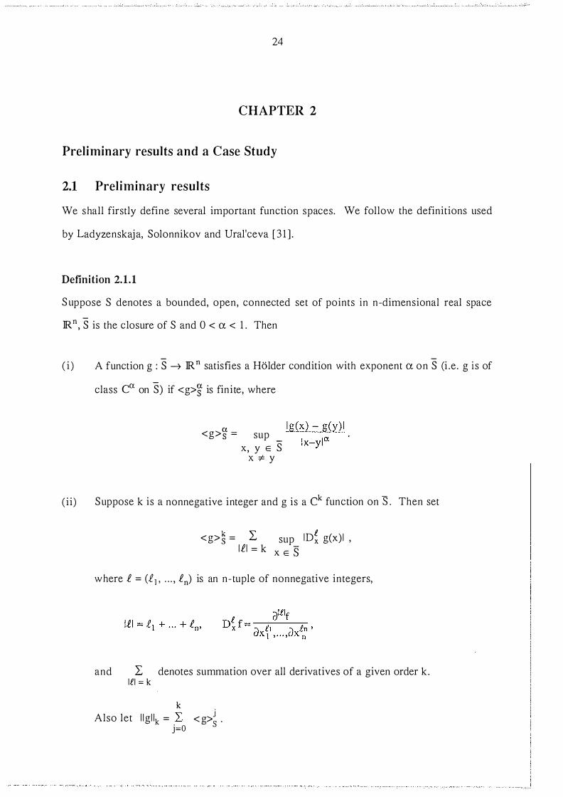
2.1 Preliminary results

We shall firstly define several important function spaces. We follow the definitions used

by Ladyzenskaj a, Solonnikov and Ural'ceva [3 1 ].

Definition 2.1.1

Suppose S denotes a bounded, open, connected set of points in n-dimensional real space

IR n , S is the closure of S and 0 < a< 1 . Then

(i ) A function g : S --1 IR n satisfies a Holder condition with exponent a on S (i .e . g i s of

class ea on S) if <g>� is finite, where

<g>� = sup _ X, y E S

X ::j:. y

lg(x) - g(y)l

(ii) Suppose k is a nonnegative integer and g is a ck function on S. Then set

<g>� = L sup ID� g(x)l , lfl = k x E S

where f = (£1, ... , fn) is an n-tuple of nonnegative integers,

and I denotes summation over all derivatives of a given order k. 1£1 = k

k � j Also let llgllk = L- <g> s .

j=O

25

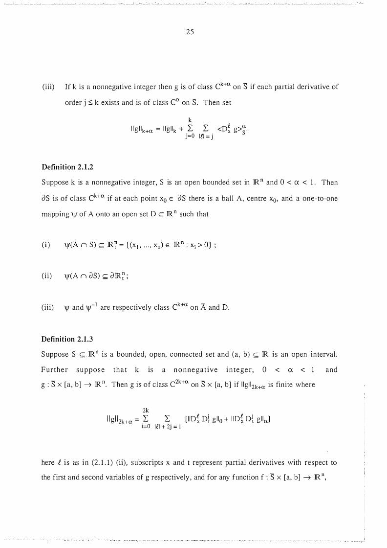
(iii) If k is a nonnegative integer then g is of class ck+a on "S if each partial derivative of

order j � k exists and is of class ea on "S. Then set

Definition 2.1.2

k l l g l l k+a = l lg l l k + 1: 1: <D� g>�·.

j=O Ill= j

S uppose k is a nonnegative integer, S is an open bounded set in lR n and 0 < a < 1 . Then

as is of class ck+a if at each point Xo E as there is a ball A, centre Xo, and a one-to-one

mapping \j/ of A onto an open set D c;;;:; lR n such that

(ii) \jf(A n as) c;;;:; aJR�;

(iii) \jf and \!f-1 are respectively class ck+<x on A and D.

Definition 2.1.3

S uppose S c;;;:;.lR n i s a bounded, open, connected set and (a, b) c;;;:; lR i s an open in terval.

Further suppose t h a t k is a n o nnega t ive i n teger , 0 < a < 1 and

g : "S X [a , b ] ---7 lR n. Then g is of class C2 k+a on "S X [a, b] if l lgl l 2 k+a is finite where

2 k l . l .

llg ll2 k+a = L L [ I IDx IYt g l lo + I IDx D{ gl l a] i=O Ill + 2j = i

here .e is as i n (2. 1 . 1 ) (ii) , subscripts x and t represent partial derivatives with respect to

the first and second variables of g respectively , and for any function f : "S x [a, b] ---7 lR n,

26

l f(x, t) - f( y,v ) l l lfl l o: = sup

- l (x, t ) - (y,v ) l o:' (x, t), ( y,v) E S x [a, b]

Definition 2.1.4

(x,t ) -:;e (y,v)

l l fl l 0 = sup lf(x ,t) l . (x , t) E S x [a, b ]

S uppose S � lR n is a bounded , open, connected set of points . For any real p ;;::: 1 , we

define the B anach space LP(S) in the u sual way to be the space consi sting of al l real

measurable functions on S with finite norm

2.1.5 The maximum principle

One of the most important results we shall use in this thesis is the maximum principle for

the solutions of differen tial e quations . We shall use the maxim um pri nciple for the

solutions of elliptic differential e quations in the following two complementary forms 0

and � .

0 S uppose that D is an open bounded set satisfying the interior sphere property of

Sperb [32] in lR n and h is a continuous non-positive function. S uppose also that w 1

is a class C2 function on D and is piecewise continuous on oD, and satisfies

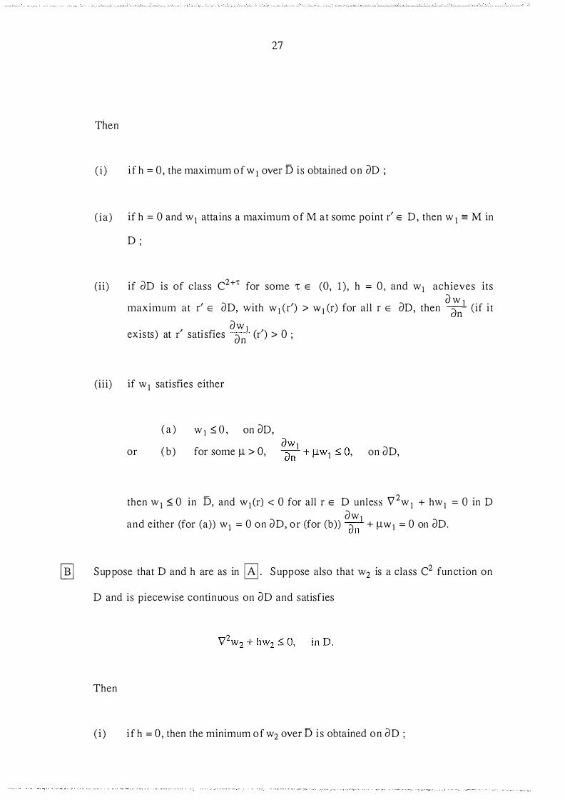
27

T hen

( i ) i f h = 0 , the maximum of w 1 over D i s obtained on ()D ;

( i a ) if h = 0 and w 1 attains a maximum of M a t some point r' E D, then w 1 = M in

D · '

(ii) if ()D is of class C2 H for some "C E (0, 1 ) , h = 0 , and w1 achieves its a w l

maximum at r ' E aD, with w l (r ') > W 1 (r) for all r E ao, then � (if i t

. ) , . f. a w 1 c ') o eXI St S at r Sat lS Ie S an r > ;

(iii) if w 1 satisfies either

or

( a ) w l ::; 0 , on ao,

( b ) for some 1-L > 0, on aD,

then w 1 ::; 0 in D, and w 1 (r) < 0 for all r E D unless \12w 1 + hw 1 = 0 in D awl

and either (for (a)) w1 = 0 on aD, or (for (b)) -::'1- + 1-LW l = 0 on aD. un

@] Suppose that D and h are as in � · S uppose also that w2 is a class C2 function on

D and is piecewise continuous on aD and satisfies

Then

( i ) i f h = 0 , then the minimum of w2 over D i s obtained on ao ;

28

( i a ) i f h = 0 and w2 attains a minimum of m a t some point r' E D , w2 =m in D ;

( i i ) i f aD i s of class C2 +'t for some "C E (0, 1 ) , h = 0 , and w2 achieves i ts a w2 minimum at r' E aD, with w2(r') < w2(r) for all r E aD, then an (if it

• ) I • f' a w2 ( ') 0 exists at r satis 1es � r < ;

(iii) if w2 satisfies either

( a ) w2 :2::0, on aD,

or ( b ) for some 11 > 0, on aD,

then w2 � 0 on D, and w2(r) > 0 for all r E D unless V2w2 + hw2 = 0 in D aw2

and either (for (a)) w2 = 0 on aD, or (for (b)) -an + !lW2 = 0 on aD.

•

For a fuller discussion of the various maximum principles see Sperb [32] and Gilbarg and

Trudinger [33] .

We shall now define the terms 'upper' and ' lower' solutions for the general elliptic

differential equation, which includes a non-local term, that we shall be discussin g in this

work.

Definition 2.1.6

Consider the nonlinear elliptic boundary value problem

V2u + f (r, u , Jn g(u)dV) = 0, r E Q,

Bu = q, r E an,

(2 . 1 )

(2 .2)

29

where B is one of the boundary operators

Bu =u,

or

Q is an open bounded set satisfying the in te lior sphere property of Sperb [32] , and, for the

purposes of this thesis, q is either zero or a piece wise continuous positive function .

The function <j)(r) i s a n upper solution for (2. 1 ) , (2.2) i f <j) i s of class C2 in Q and satisfies

S imilarly the function \jf(r) is a lower solution for (2. 1 ) , (2.2) if \If is of class C2 in Q and

sat i sfies

B \jf � q, r E CJQ. Ill

The existence of upper and lower solutions can be combined with the maximum principle to

show that el l ip tic boundary val ue problems of the form (2. 1 ) , (2.2) have a solution . The

result we wil l use here can be considered to be a generalization of Sattinger 's [ 3 4] result

concerning the case g(u) = 0. The proof we will use is similar to that of Sattinger' s except

a Frechet derivative is introduced to extend the results to non-zero g(u) . The proof is

given in detail both for the sake of completeness and as it i l lustrates the method of

monotone i teration inherent in many of the results in this thesis.

30

Theorem 2.1.7

S uppose there exists an upper solution <j>0(r) of (2. 1 ), (2.2) and a lower solution 'Jfo(r) of

(2 . 1 ) , (2.2) with <j>0(r) :2: \jfo(r) for r E .Q. Then there exists a regular solu tion u (r) of (2. 1 ) ,

(2.2) such that

Proof

We will assume that we can find a positive constant e so that the function

F (r, u, In g(u) dV) = f (r, u, In g(u) dV) + eu,

is an increasing function of u.

Now F (r, u, fn g(u) dV) will be an increasing function of u if the corresponding Frechet

derivative i s positive. To explain what is mean by the Frechet derivative of F, we will

consider the non-local term in the function which maps u -t In g(u) dV to be given by

k(u) = In g(u) dV.

The Frechet derivative of f(r, u, k(u)) for a small positive perturbation h(r) is defined to be

J(u) (h) where

f(r, u+h, k (u+h)) - f(r, u, k(u)) = J(u)(h) + o(llhll) .

Now

31

df df J(u) (h ) = du (r, u, k) h + dk (r, u, k ) K(u)(h ),

where K(u)(h) is a 'complementary' Frechet derivative satisfying

k(u+h) - k(u) = K(u) (h) + o(llhll),

i.e.

K(u)(h) = In � h dV.

Obviously if g(u) = 0, the requirement on e reduces to

df dU (r, u) + e > 0, (c.f. Sattinger [34]),

otherwise i t is sufficient that e satisfies, for all small positive perturbations h,

J(u)(h) + 8h > 0, r E Q.

Having found such a 8, define a mapping T : \If= T<P if

B\lf = q, r E an.

32

Now T is completely continuous and monotone, i.e. , \jf � max <j>0. To show this monotonicity consider =- [ f (r, <j> , fn g(<j>) dV) + 8<!>] , r E n,

(V2 - 8)T\jf =- [ f (r, \jf, fn g(\jf) dV) + 8\jf] , r E n,

BT<j> = BT\jf = q, r E an.

(\72 - 8) (T\jf - T<j>) =- [ f (r, \jf, In g(\jf) dV )- f (r, <j>, In g(<j>) dV)

If we now define

+ 8(\jf - <P) } r E n

B(T\jf - T<j>) = 0, r E an.

F (r , u , In g(u) dV )= f (r, u , In g(u) dV) + 8u,

(2 .3 )

then F has a positive Frechet derivative and so is increasing in u. So the terms in the

square brackets on the right hand side of (2.3) combine to form

F (r, \jf, Jn g(\jf) dV )- F (r, <j> , In g(<j>) dV) � 0.

This implies

33

( \72 - E>)w s; 0, r E n,

Bw = 0, rE an,

where w = T\jl- T<)>. So by the maximum principle [ill, w > 0 in n, and hence T'lf > T<)> in

n .

Now define <)>1 = T <)>0 and \jf 1 = T'lfo (where <)>0, 'Vo are respectively the upper and lower solutions of (2. 1 ) , (2.2)) . We will now show that <)>1 < <l>o and \jf 1 > 'Vo· We have

s o

and

B <)>l = q, r E an,

( \72 - E>)(I- <l>o) =- f (r , <l>o . L, g(<l>o) dV )- E><!>o- V2 <l>o + E><!>o,

=- [ V2 <)>0 + f (r, <)>0, Jn g ( <)>0) dV) ] ,

� 0, rE n,

34

Therefore by the maximum principle �, <1> 1 < <l>o i n Q. Furthermore since \jf 0 :::;; <Po it

follows by the monotone property of T that T \j/0 < T<j>0 i n Q, that is, \jf 1 < <j> 1 .

So we have

Now define <1>2 = T<j>1 . Since <1> 1 < <j>0, we have T<j>1 < T<j>0 in Q , that i s <1>2 < <j> 1 . A l so i f we

define \j/2 = T \j/1 , then \j/2 > \j/1 in Q. S ince \j/1 < <!> 1 it fol lows that T \!f1 < T<j> 1 i n Q, so

\j/2 < <j>2. So we have

Continuing i n this manner we obtain the sequences { <PJ, { o/J satisfying

Since the sequences { <PJ, { \j!J are monotone and bounded, both converge pointwise. Let

these l imits be (!) (r) and \j/(r) respectively where

(!) (r) = lim <l>i(r) , \j/(r) = lim \jfj(r) . i --7= i --7=

The operator T is a composition of the nonlinear operation <1> l--7 f (r, <j>, fo g(<j>) dV) + 8<!>

with the inversion of the linear, inhomogeneous el l ip tic boundary value problem X l--7 \jf

defined by

35

B'Jf = q, r E ()Q

For <1> and f (r, <!J, Jn g(<!>) dV) bounded on the range of <!J, the first operation takes bounded

pointwise convergent sequences into poin twise convergent sequences . The operation X

l--7 'V takes Lp(Q) continuously in to the Sobolev space W2, p(Q) for all p , 1 < p < oo (by

the LP estimates of Agmon et al [35]) . So since <Pi = T<Pi-1 and since { <Pd is a bounded

pointwise convergent sequence, it converges also in W2, p· By the embedding lemma [35],

W 2, P i s embedded continuously into cl+a, and by the classical Schauder estimates for

regular elliptic boundary value problems ( <Pd then also converges in c2+<x. So we have

and similarly

�(r) = lim <P/r) = lim T<Pi-l (r) = T lim <Pi-1 (r) = T� (r) , i�oo i�oo i�oo

\f!(r) = lim 'Vi(r) = lim T \Jfi_1(r) = T lim 'Jii_1(r) = T \f!(r) . i�oo j�oo i�oo

So (j) and \jl are fixed points of the mapping T, and are of class c2+<\Q) for 0 < a < 1 .

Thus (j) and \jl are solutions of (2 . 1 ) , (2.2) . Therefore (2. 1 ) , (2.2) has at least one solution

between <Po and \Jfo· This completes the proof.

•

We shall make use throughout this thesis of the function w(r) which satisfies:

with either

or

Theorem 2.1.8

aw -+11w = O dn �'"" '

36

r E an,

(where an i s Of cla SS C2 H for SOme 't E (0, 1 )) ,

w = O, r E an.

Suppose the function w(r) sati sfies (2.4) in n.

Then

( i )

( i i)

Proof

w(r) > 0 ,

dw (r) 0 � < ,

r E n,

r E dn.

Directly from the maximum principle @].

Theorem 2.1.9

Consider the problems

( a )

and

( b )

W5 = 0, r E aS ,

w d = 0 , r E a n,

where S , D are regions satisfying the interior sphere property of Sperb [ 32 ].

(2 .4)

37

Then if S � D, i .e. S is wholly enclosed by D,

Proof

Assume there exist points i n S such that w5 > w d. Then, since w d and w5 are positive in S

by Theorem 2. 1 . 8 , there exists a positive constant k < 1 such that

kw5 < w d for r E S/r',

kw5 = w d at r = r' E S ,

(2 .5 )

(2 .6 )

( i f there exists more than one such poin t r' , we choose just one of these points in the

fol lowing argument) . Therefore kw5 - w d has a maximum of zero at r = r' . But

V2(kw5-w d) = -k + 1 > 0 everywhere i n S and in particular at r = r', so by the maximum

principle � ' kw5 - w d = 0 for all r E S . This i s a contrad iction of inequali ty (2 .5) .

Therefore w d 2:: W5, r E S .

Theorem 2.1 .1 0

Let D � IR 3 be any convex shape with aD of class C2 +'t for some 1: E (0, 1 ) , and S be a

sphere (of radius a) wholly enclosed by D . If we consider the problems

( a )

and

av an + flv = O,

r E D,

r E aD,

38

( b ) V2w5 + 1 = 0, r E S ,

aw s On + jlWs = 0, f E CJS ,

with ll > 0 ,

t hen V;::: W5, r E S .

Proof

Figure 2.1 Convex shape with enclosed sphere

Let 0 be the centre of the sphere, P be a point on aD, Q be on the tangent to aD at P such

that PQ is perpendicular to OQ, Q' be a point on OQ which is also on oS, and let 8 be the

angle between OQ and OP. It is well-known that the solution to (b) is

a2 - r2 w s (r) = 6

39

a + -

3 �, r E S . (2 .7 )

Now we can easily extend w5's domain to D , as w5 satisfies the same equ ation i . e.

V2w 5 + 1 = 0. Consider the new boundary vo..lue

Now at P ,

and

So

dw s -OP ar= 3 ,

but OQ � a , (for a l l P since D is a convex shape and OQ � OQ' = a)

and OP � a,

which gives

We finally consider the function v - w5 (again extending w5's domain to D),

40

which gives, by the maximum principle � ' v :2: w5, r E D, and in particular

Ill

Corollary 2.1.11

For the region D and function v defined in Theorem 2. 1 . 10, there exists Gtn E > 0 such that

Proof

v :2: E, for all r E D.

Considering the vector £ to be a position vector in 3- space, define the sphere S s with

centre Is to be

Now as D is convex, there is a 8 > 0 such that V£ E D, there exists a sphere S s such that

r E S s. Then by (2.7) and Theorem 2. 1 . 10 ,

8 v :2:- > 0, Vr E D.

3fl

Ill

The result stated below may well be a standard result from d i fferenti al e qua tio n theory,

but we present a proof here for complete ness.

4 1

Theorem 2.1.12

S uppose there exists a function <P which is of class C2 on a region Q c IR 3 arld satisfies

Then (£) does have a minimum at £ = r', and \7 2<1> (£ ') < 0. The Taylor series

expansion of <PC£) about £ = ( is

where A i s the Hessian matrix of (() = Q) ,

hence A is a semi-positive definite matrix with

This contradicts our original statement regarding the sign of \72<j>(r ') and so completes the

proof.

2.2 Industrial Case Study

2.2.1 Background

42

In thi s section we wi l l consider i n deta i l the i nvesti gation of a particular i ndus trial fire

caused by spontaneous i gn i tion . B y u si ng the experimentally measured physi cal

parameters of the materials involved, we shall predic t a safe s torage (or in this case,

cleani n g) regi me which should prevent s imi lar fires from occurr ing i n the same

environment. The fire i n question was caused by the self-heating to igni t ion of a wood

fibre dust layer on a hot factory press. S ince the typical press operating temperature was

approximately 200°C, this fire comes under the first of the two categories of spontaneous

combustion fires outlined i n the in troduction i .e. where a small body of material is stored

subject to high ambient conditions. S ince the hot surface temperature i s above 1 00°C we

wil l assume that there is no moisture and there are no microbes presen t in the self-heating

dust layer (the maximum temperature commonly recognised as an upper l imit for l iving

processes is 75 - 79°C (Kempner [36] ) ) . Therefore we wil l assume the self-heating of

the body i s due to a s ingle exothermic process i .e. direct chemical oxidation, so that the

analysi s of the model can proceed by the s ingle Arrhenius term approach . The problem

can be treated as a self-heating body subject to asymmetric boundary condi tions. We will

compare the results obtained using three different approaches, all of which solve for the

steady states (dT/d1 = 0) of the classical problem ( l . l a, b, c), ( 1 .2) . Firstly by the

method of Thomas and Bowes [ 8 ] , which uses the Frank-Kamenetskii approximation to

the Arrhenius term and assumes the dust layer can be approximated by an infi n ite slab.

S econdly by a method which retains the ful l Arrhenius kinetics but also assumes the body

i s an i nfin i te slab. For this method we use the new dimension less formulation of Burnell

et al [ 1 2] , this approach has also been studied by S houmann and Donaldson [9] using the

classical Frank-Kamenetskii dimensionless formulat ion . Finally we shall use a method

which solves the full problem: ful l Arrhenius k inetics in the three dimensional domain. By

43

these comparisons we hope to answer some of the following questions that arise m

practical situations using ignition theory.

( i ) how well does the Frank-Kamenetskii approximation behave in practice?

(ii) when does the infinite slab approximation for a rectangular block fail to be valid in

ignition theory?

(iii) what are the upper and lower bounds for the s teady s tate temperature profile

beyond cri ticality for models retaining the ful l Arrhenius kinetics?

We will comment on the suitability of Newtonian cool ing versus perfect heat transfer

boundary conditions for this particular problem. Finally we shall show that the minimal

positive solutions for UP < Up, crit for both the ful l Arrhenius term models is stable. We

shall do this by a non-trivial extension of the approach of Keller and Cohen l37] . We must

make this adaptation since, u nlike Keller and Cohen' s [37] system, our bifurcation

parameter UP occurs in the boundary conditions for the model. This work has been

published, see S isson , Swift and Wake [ 10] .

At this stage we shall give a more detailed outline of the conditions i n the factory under

which the fire occurred.

A New Zealand company which produces medium density fibreboard from pine woodchips

noticed several unexplained fires occurring on the presses in their factory (on average two

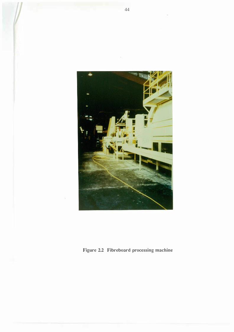
per year) . Figures 2 . 2 - 2 .4 below show, respectively, the fibreboard processing machine

within the factory, the fibreboard press itself, and the finished product - medium density

fibreboard.

44

Figure 2.2 Fibreboard processing machine

45

Figure 2.3 Fibreboard press

46

Figure 2.4 Medium density fibreboard

47

Figure 2 .5 below gives a schematic representation of the press operation in the factory .

3 metres "

fibreboard

CONVEYOR BELT

· 1 0 metres

press woodfibre

Figure 2.5 Schematic diagram of fibreboard press

The press itself was heated by thermal oil usually at a temperature of 200°C (subject to

fluctuations) . During its normal operation deposits of mixed fibre and oil built up as dust

layers on various parts of the press. The company required the possible cause of the fires

due to spontaneous ignition of these dust layers to be investigated, given that the normal

'ignition temperature' of the fibre/oil substance was well in excess of 200°C. The results

would be used to implement efficient c leaning procedures (the press operated 24 hours per

day, being shut down only for cleaning) . On a visit to the factory made by one of the team

of investigators , it was observed that the fibre/oil mixture was escaping from the conveyor

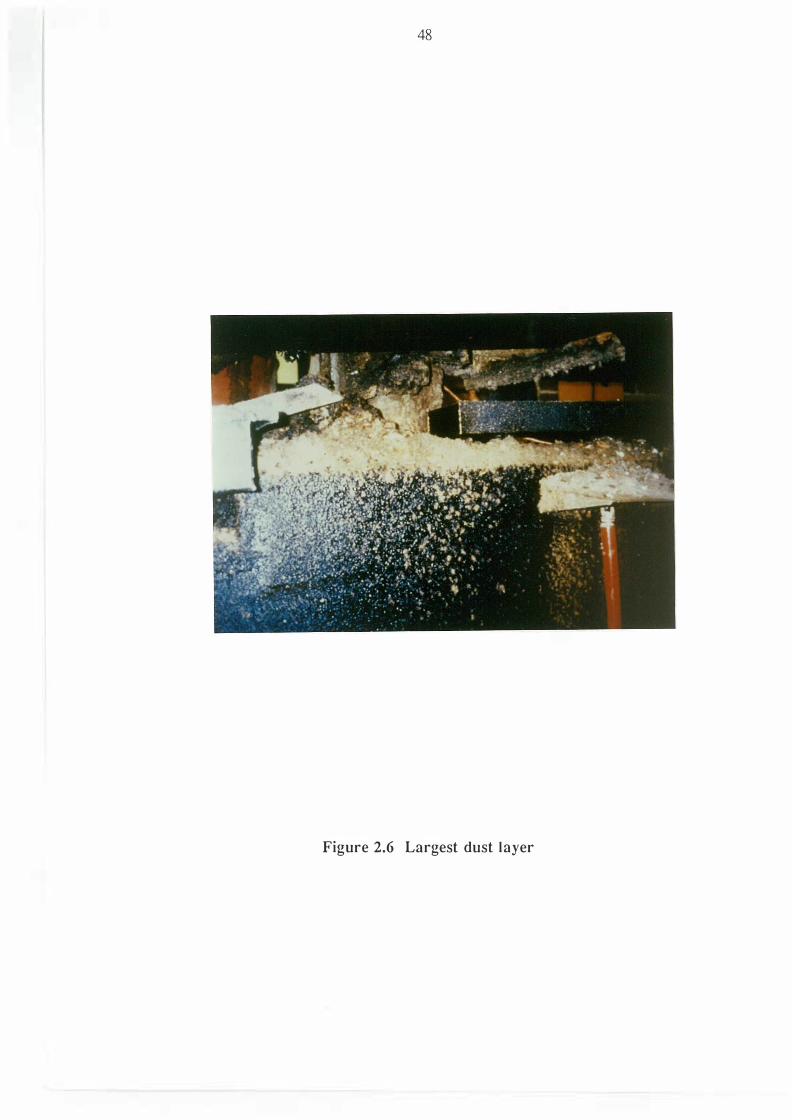
belt and building up on shelves inside the press casing. The largest of these dust layers is

shown in Figure 2 .6 below.

48

Figure 2.6 Largest dust layer

49

This dust l ayer was observed to be a rectangular block of fixed base 50cm x l OOcm. The

height of the dust l ayer (ah) was measured to be a maximum of 20cm on the d ay of the

visit. The block is shown schematically in Figure 2.7 below.

50 cm

Figure 2.7 Schematic d iagram of l argest dust layer

The problem then , is to estimate the maximum height of the rectangular b lock (as a

function of the press temperature) , such that the dust layer is not likely to self- heat to

ignition.

2.2.2 Boundary condit ions

The block shown in Figure 2.7 does not satisfy the ' interior sphere' property (see Sperb

[32] ) . So in order to use maximum principle � (part (ii)) we consider a similar block

with 'rounded corners' . This will have negligible effect on the nature of the bifurcation

diagrams and the results that follow (see e.g. Fradkin and Wake (3 8]) .

50

In this section we wil l consider the suitable boundary conditions for the press/dust layer

i nterface. The boundary conditions for the dust layer/air interface will be discussed further

in a later section in this Chapter. If, provisionally, Newtonian cooling boundary conditions

are taken at each interface, then the boundary conditions become

oT k2 on + h1 (T-Tp) = 0, at the press/dust layer interface, (2 . 8 )

oT k2 on + h2 (T-T a) = 0, at the dust layer/air interface, (2.9)

w here

k2 = thermal conductivity of the fibre/oil dust layer,

h l = heat transfer coefficient for the press/dust layer interface,

h2 = heat transfer coefficien t for the dust layer/air interface,

TP = absolute temperature of the press,

Ta = absolute ambient temperature in the factory (taken as a fixed 300K),

also

k l = thermal conductivity of the press,

k3 = thermal conductivity of air.

I n their paper Thomas and Bowes [8] assumed perfect heat transfer between the hot

surface and the slab body , that is h1 ---7 oo. This gives the boundary condition at the

press/dust layer interface as

(2 . 1 0)

5 1

Actual v alues of k1 and k2 are unavailable, but typical values (Jones [39]) would be

kl = 47 Wm-1 K-1 ,

kz = 0 . 1 03 Wm-1 K-1 ,

a l so

k3 = 0.026 Wm-1 K-1.

Given that k 1 >> k2 , and h 1 i s dependent on the ratio of these, Thomas and Bowes'

assumption seems to be valid for th is model . Thus we will also use (2. 1 0) as the

boundary condition at the press/dust layer in terface. The difference between k2 and k3

however, and so the appropriate boundary condition at the dust layer/air interface, is less

well defined.

2.2.3 O u tline of Thomas and Bowes' method

The application of the paper of Thomas and Bowes [81 assumes that two important

simplifications can be made to the model: (a) the rectangular block can be approximated

by an infinite slab; (b) it is valid to make the Frank-Kamenetskii approximation based on

the press temperature T P' i .e .

exp (-RET) "" exp( -E ) exp(E(T-Tp))

RTP RT/ .

Under these assumptions the equation for the s teady s tates of ( l . l a) , ( 1 . 2 ) with the

boundary conditions (2.9), (2. 1 0) becomes

0 < X < 2,

8 = 0, at X = 0 , (2 . 1 1)

at X = 2,

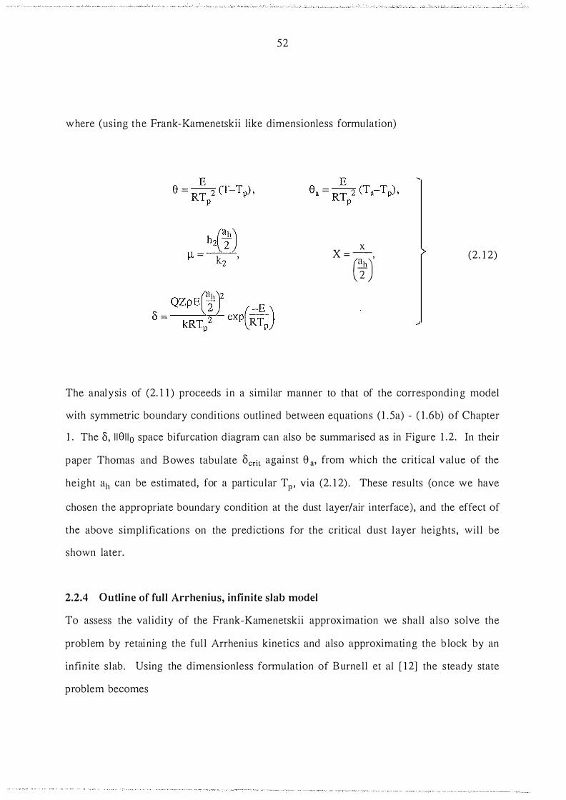
52

where (using the Frank-Kamenetskii like dimensionless formulation)

X X = -

Ci) (2. 1 2)

The analysis of (2. 1 1 ) proceeds in a similar manner to that of the corresponding model

with symmetric boundary condi tions outlined between equations ( 1 . 5a) - ( 1 .6b) of Chapter

1 . The 8, 1 1 8 1 1 0 space bifurcation diagram can also be summarised as in Figure 1 .2. In their

paper Thomas and Bowes tabulate ocrit against 8 a, from which the critical v alue of the

height a11 can be estimated, for a particular TP , via (2. 1 2) . These results (once we have

chosen the appropriate boundary condition at the dust layer/air interface), and the effect of

the above simpl ifications on the predictions for the critical dust l ayer heights, wi l l be

shown later.

2.2.4 Outline of ful l Arrhenius, infinite slab model

To assess the validity of the Frank-Kamenetskii approximation we shall also solve the

problem by retaining the ful l Arrhenius kinetics and also approximating the b lock by an

infinite s lab. Using the dimensionless formulation of Burnel l et al [ 1 2] the s teady state

problem becomes

53

0 < X < 1 ,

at X = 0 , (2. 1 3)

: + Bi(u-Ua) = 0 , a t X = I

where

RT RTP RTa u = E , u = E , Ua = E , p

(2. 1 4) pQAR(a11)2 X . h2 ah

11 = kE X = - BI = k;-ah ,

Here 11 is a constant (for a given a11) and the bifurcation (distingu ished) parameter is taken

as UP, the dimensionless temperature of the press . No exact solution is known for (2. 1 3)

so i t must be solved by numerical means. The numerical algorithm used i s similar to that

outlined for the three dimensional model in Sec tion 2 .2 .8 l ater in this Chap ter. A

schematic example of a typical bifurcation diagram i n UP, � space (where � is the

temperature of a typical poin t in the domain) for a model which retains the ful l Anhenius

kinetics is given below in Figure 2.8 .

� = temp. of typical

point in domain

54

up, crit

Figure 2.8 Schematic diagram of a typica l UP, � bifurcation diagram for the ful l

Arrhenius, infinite s lab model

For UP > Up, crit there exists a high temperature steady state profile. This bifurcation

diagram can be compared with that of Thomas and Bowes [8 ] (Figure 1 .2) which predicts

no steady state solutions beyond criticality. This larger steady state i s ' lost' due to the

Frank-Kamenetskii approximation to the Arrhenius term. Later in this c hapter we shal l

verify that this s teady state is so large that ignition wi l l have occurred ' long' before i t i s

ever reached in a time sense.

55

2.2.5 Measurement of physical constants rela ted to the model

Experimental analysis was performed on samples of the fibre/oi l material (Smedley [ 40])

using methods similar to those outlined in the introduction. This analysis yielded

pQAR 14 -2 kE = 4.23 X 1 0 m ,

E R = 1 6220 K.

The actua l v al ue of the dust layer/air heat transfer coefficient was unavailable, but, given

that a typical value of a wall/air heat transfer coefficient in sti l l air is 8 . 3 wm-1 K-1 (Jones

[39] ) we wil l take

2.2.6 The boundary condition at the dust layer/air interface

In section 2.2.2 above we j ustified the boundary condition T = TP at the press/dust layer

interface. Here we wil l test the hypothesis that h2 --1 oo is also a valid assumption for the

model, i .e . that the boundary condition at the dust layer/air interface can be taken as

We will use the method in section 2.2.4 (infinite slab, full Arrhenius model) with

i .e . T = Ta at the dust layer/air interface,

(2 . 1 5 )

and

i .e .

56

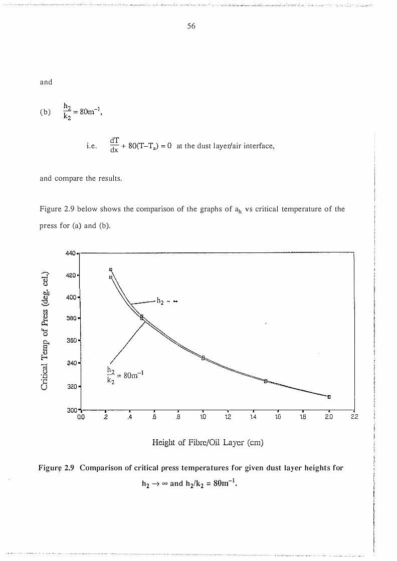
dT dx + 80(T-Ta) = 0 at the dust l ayer/air interface,

and compare the results.

Figure 2.9 below shows the comparison of the graphs of ah vs critical temperature of the

press for (a) and (b).

440

--;. 420 ........ � bb 400 �

� � 0

� <U � � u ·.o ·c: u

300 0.0 2 .4 .6 .8 1.0 l2 1.4 lG 1.8 2.0

Height of Fibre/Oil Layer (cm)

Figur� 2.9 Comparison of critical press tempera tures for given dust layer heights for

h2 -t 00 and h2/k2 = som-1 •

2.2

57

The comparison suggests that for the practical range of a11 (� 2cm) and T P ( <573K) the

critical press temperatures corresponding to the two boundary condi t ions are

indistinguishable. The tabulated results in Thomas and Bowes paper also indicate that

h2 ---7 oo is a good approximation for this model. Consequently our final steady state model

on which the analysis of all three methods wil l be based is the steady states of ( 1 . 1 a),

( 1 .2) with the boundary conditions (2. 1 0) , (2. 1 5) .

2.2.7 Existence of solutions to the ful l Arrhenius model

In this section we wil l verify the existence of at least one solution for all UP > 0 (in

p articular UP > Up, crit) for the models which retain the ful l Arrhenius kinetics (i .e . both the

infi ni te s lab and the ful l three dimensional domains) . We wil l also show, us ing the

maximum principle, that any solution of the model must occur between the constructed

bounds.

Theorem 2.2 . 1

Consider the problem

u(an') = Ua,

u(an") = UP '

i n n,

an' u an" = an,

Tl > 0 .

There exists a solution u to this problem for a l l UP > Ua > 0, sati sfying

w here w satisfies (2.4) with w(an) = 0.

(2 . 1 6)

Proof

Let

then

and

S o

A lso let

then

and

So

58

\jf(r) = Ua r E Q,

V 21Jf + 11 exp( ��: ) � 11 expfu:) in Q,

� 0,

\jf(r) = U a is a lower solution of (2. 1 6) .

<j>(r) = Up + 11W(r) , r E Q,

::; 0,

<j>(r) = UP + 11 w(r) , r E Q, is an upper solution of (2. 1 6) .

A lso since UP > U a• <j> (r) > \jf(r) in Q. So by Theorem 2. 1 . 7 , there exists a solu tion u of

(2. 1 6) with

59

Corol lary 2.2.2

Setting <j> = UP + 11w - u and \jf = u - Ua, and applying the maximum principle �' it can

easily be shown that <j> � 0 and \jf � 0 i n .Q. Therefore any solution u of (2. 1 6) must satisfy

2.2.8 Three dimensional model and outline of the numerical a lgorithm

Again using the dimensionless formulation of Burnell et al [ 1 2] , the three dimensional

version of the steady state problem becomes

with

in .Q,

U = Ua , on the dust layer/air interface ,

u = up ' on the dust l ayer/press in terface.

The dimension less variables are defined as in (2. 1 4) with the additions

(2. 1 7 )

(2. 1 8 )

Using three term difference approximations to the second derivatives in the three

coordinate directions, and a suitable three dimensional fin i te difference mesh to represent

the domain , (2. 1 7) reduces to a system of non-linear equations of the form

F ( a , �) = O , � � �

(2 . 1 9 )

60

where � is the vector of unknown temperatures at the internal mesh points (excluding �) ,

and � (which wi l l take the role of a path following parameter) i s the temperature a t an

arbitraril y chosen mesh poin t in the domain . This system is solved (for a particular a11) by

defining � to be some given �0 and then solving the resulting well-posed system for the

u nknown temperature vector � = �(�0) by a Newton-Raphson method (which involves the

calculation of the Jacobian matrix for f) . We can then solve (2 . I q ) for � (�0+1'1�) by a

combined Euler predictor and Newton corrector scheme. This approach is similar to that

used by Abbot [41] . In particu lar UP is thus calculated for a range of values of �· As �

can be thought'of as a characterisation value for the domain temperature profile, a plot in

U p C�) , � space wil l represent a s teady state bifurcation diagram for the system for a

particular a1l' The graph is plotted in this manner since physically UP is the control variable

and � the response. The critical value of UP, i .e. Up, crit can then be observed from the

graph i n the usual way. It is expected on physical grounds that the value of Up, crit should

be independent of the point at which we choose to define �' but we have been unable to

find a rigorous proof of this.

2.2.9 Existence and bounds for h igher steady state

In this section we will prove the existence of, and derive bounds for, the higher steady

state solution the temperature will approach (in a time sense) beyond criticality. We will

do this for the two models which retain the ful l Arrhenius term. Our aim is to show that

this 'passage of up through criticality' is sufficient to induce thermal ignition in the body.

We achieve this by showing that the steady state temperature a typical point in the body

wil l approach is very high indeed (> 1 0 10 °C).

I t is obvious that in most physical situations ignition will occur long before this higher

steady state is attained; thus in terms of physically observed behaviour predicted beyond

criticality, there is no difference between these models and the Thomas and Bowes model

6 1

(which predicts no higher s teady state beyond cri tical i ty) , i n realistic s i tuations .

However, although this s teady s tate is not physically realizable, it is an important factor

for the set of differen t i ni tial conditions, which arise in , for example, the question of hot

assembly (see Gray and Wake [42] ) .

2.2.9.1 Existence

I t can be shown, usmg methods similar to those u sed by Wake e t al [ 1 3 ] for the

symmetrical heating case, that for 11 'sufficien tly large' (2. 1 6) has

( i ) an upper solution <j} = Up + 'llW,

(i i) a lower solution \If = Ua + exp(Aw .t'n'll )-1 ,

with <P � \If i n Q,

where w is the solution of (2.4) with w(oQ) = 0, and A = 2 1 1� 1 1 0 .

In this context, 11 'sufficiently large' corresponds to 11 satisfying the following inequalities

( i )

(ii )

(iii)

( iv )

1 .t'n11 > Ak ' 1

exp(A.t'1 .t'n'll ) > 2 ,

-{;\ > Ae .t'n'Jl ,

-{;!- 1 1l > l l w l l0 '

(2 .20)

62

where k 1 , £ 1 are constants satisfying

with

We wil l not give the detail s of this result at this stage, as this approach wil l be used again

later in this thesis, and these inequalities will then be derived ful ly , (in Chapter 5 ) .

B y Theorem 2. 1 .7 there then exists, for 11 satisfying the i nequalities (2.20), a solu tion u of

(2. 1 6) with

Ua + exp(Aw .ln11) - 1 s:; u s:; UP + 11W, in Q. (2 .2 1 )

This solution corresponds to the very high steady state. To obtain bounds for this steady

s tate, or at least for a typical poin t in the profi le, we must solve (2.4) (with w(o.Q) = 0) in

the particular domain .

2.2.9.2 Bounds on the higher steady state for the ful l Arrhenius, infinite s lab model

To derive bounds for the higher steady state for an i nfin ite slab of height ah we must solve

the one dimensional linear ordinary differential equation

w = 0, at X = 0,

w = 0, at X = 1 .

63

This has the simple analytic solution

w (X) = X ( l-X)/2.

Now, since

for ah in the range of interest, i .e. a11 ;:::: 5cm, we can assume

For w given i n (2.22) , that is with

we can choose Qk2, Q.e2 such that

l lw l l 0 = 0 . 1 25 , A = 4 ,

w ;:::: £2 = 0.0 1 ,

(2 .22)

(2 .23)

(2.24)

) (2 .25)

Substituting these values i nto the inequali ties (2.20) we see that a l l are satisfied since

( i ) 27 .67 > 1 .09,

( i i ) 3 .02 > 2,

( i i i ) 1 . 02 X 1 06 > 301 ,

( i v ) 1 .05 X 1 01 2

> 8 .2 X 1 06.

64

So , i ndeed, for the range of a11 of i nterest, and for w given i n (2.22), 11 i s sufficiently large

so that <j> and \jf given i n section 2 .2.9 . 1 are upper and lower solutions respectively for the

i nfin i te slab, ful l Arrhenius model . Now let us define �* ( in degrees Celsius) to be the

temperature which the (dimensionless) temperature � of the typical poin t in the domain

approaches for up > up, criv

Then, for example, for an infi nite s lab of height 5cm, and a typical point chosen at the

'centre' of the slab ( i .e . X = 0.5) , this approach gives the following bounds on �*

1 .65 X 10]() °C ::; �* ::; 2. 1 2 X 1 01 5 °C.

2.2.9.3 Bounds on h ighet· steady state for ful l Arrhenius, three dimensiona l domain

model.

Obtaining bounds via (2.20) i nvolves solving the equation

w({jQ) = 0,

where Q is a 'brick' of base 50cm x 1 00cm and height a11• G iven that we must simply show

that the lower bound is sufficiently large to induce ign i tion, an acceptable method of

obtaining bounds for this problem can be found by using the solutions for w in the inscribed

65

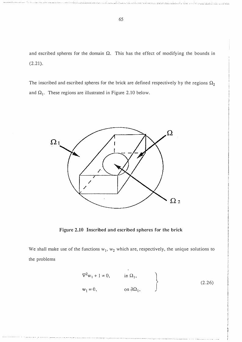
and escribed spheres for the domain Q. This has the effect of modifying the bounds in

(2. 2 1 ) .

The inscribed and escribed spheres for the brick are defined respectively by the regions Q2

and Q1 . These regions are illustrated in Figure 2. 1 0 below.

Figure 2.10 Inscribed and escribed spheres for the brick

We shall make use of the functions w1 , w2 which are, respectively, the unique solutions to

the problems

} (2 .26)

66

and

} (2 .27)

and also of the following Theorem.

Theorem 2.2.3

If w, with w(o.Q) = 0, w1 and w2 are respecti vely the solu tions of (2.4) , (2.26) and (2.27)

then

Proof

S imple application of Theorem 2. 1 . 9 .

By Theorem 2.2. 1 and Corollary 2.2 .2 the solution u of (2. 1 5) , and in particu lar the portion

of the u profi le i nside .Q2, exists and satisfies

with

U a ::;; u(r) ::;; Up + w(r), r E ().Q2·

Now consider the solution of

where q 1 (r) i s an unspecified function satisfying

We will show that

is an upper solution of (2.28) .

Now

and

so indeed <P is an upper solution .

67

u (r) = q1 (r) , r E ()Q2, (2 .28)

68

Also

1 i s a lower solution of (2.28) for the part of u inside Q2 , where A2 = 2 1 1w2 1 10 and 11 i s

sufficiently large so that i t satisfies the fol lowing inequal ities

1 ( i ) fn11 > A k ' 2 3

( i i ) exp (A2£3 fn11 ) > 2 ,

--{n > A2e fn11 , (2 .29)

(iii)

( iv) f;l- 1

11 > l l w2 1 10 '

and where k3 , £3 are constan ts satisfying

with

Again, the detai ls for the verification of this lower solution will be given later in the thesis.

It should be noted that \jf satisfies the correct boundary inequality to be a lower solution

since, on an2

69

In the inscribed sphere of radius l , (2.27) reduces to

which has the analytic solution

w�( 0 ) = a,

_1 2 w2 = 24 ( l -4r ) .

I n the escribed sphere, which has radius ... I � ( 1 + �) , (2.26) reduces to -\1 4_ah

2 d w 1 2 dw 1 -- + - - + 1 = 0 dr2 r dr ' 0 < r < - I ± ( 1 + �) , . \f 4_gh

which has the analytic solution

0 ) = o, l (l +-5 ) = 0 4 4a 2 '

-h

1 ( 5 2) wl = 24 1 + 4_gh2 - 4r '

where _a11 is the dimensionless length of a1r

(2 .30)

(2.3 1 )

70

. 1 Now (2.30) giVes l lw2 1 10 = 24, A2 = 1 2 and we can choose £3 = 0.0 1 , k3 = 0.02 1 1 , hence 11

satisfies a l l the inequalities (2.29). Choosing the typical point � to be the centre of the

escribed sphere, we obtain the following bounds for �* (i .e . the temperature of the typical

point in degrees celcius) for the three dimensional brick with dust layer height 5cm.

These resu lts can be used to derive bounds for the higher steady state for any point within

.Q2, and they indicate that the higher steady state solu tion is indeed sufficient ly l arge in

magnitude to induce ignition in the body.

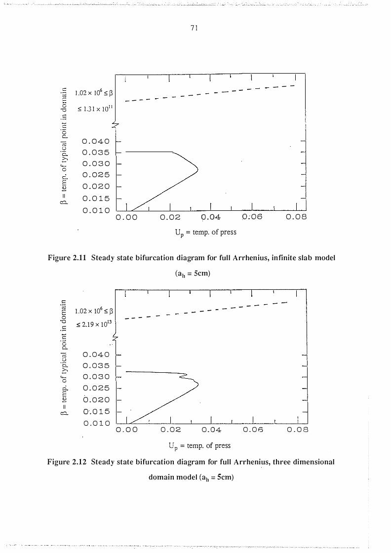
2.2.10 Example steady state bifurcation diagrams

In the example steady state bifurcation diagrams given below, the bold sections have been

computer generated and the broken sections correspond to the higher s teady s tate the

system will approach for up > up, crit (derived by appealing to the bounds in section 2.2.9).

Figure 2 . 1 1 corresponds to the steady state bifurcation diagram obtained for the ful l

Arrhenius, infinite slab model for a 5cm high dust layer with typical point � chosen at the

'centre' of the i nfinite slab. Figure 2. 1 2 corresponds to the bifurcation diagram obtained for

the ful l Arrhenius, three dimensional for the dust l ayer of height 5cm, with � chosen at the

centre of the inscribed sphere.

71

- - -,.... 1 .02 X 106 ::::.; � - - -

- - - -..... - - -..... 0 ::s; l .3 l x l01 1 -o ..... ....... ..... 0 c.. 0 . 0 4 0 .w

:..> 0 . 0 3 5 c.. c 0 . 0 3 0 "'-0 c.. 0 . 0 2 5 ..... ..... 0 . 0 2 0 � 1 1 0 . 0 1 5 �

0 . 0 1 0 0 . 0 0 0 . 0 2 0 . 04 0 : 0 6 0 . 0 8 up = temp. of press

Figure 2.11 Steady state bifurcation diagram for ful l Arrhenius, infinite slab model

(a 11 = Scm)

.5 - -:-;:: 1 .02 X 106 ::::.; � - - - - -,... - - - - -c: 0 - - - - -

-o ::::.; 2. 1 9 X 1013 c::

· � ....... c:: 0 c.. :-;:: 0 . 04 0 :..> ·c. c 0 . 0 3 5

"'-0 0 . 0 3 0 c.. 0 . 0 2 5 ,... c: 2::: 0 . 0 2 0 1 1 o·. o 1 5 �

0 . 0 1 0 0 . 0 0 0 . 0 2 0 . 04 0 . 0 6 0 . 0 8

UP = temp. of press

Figure 2.12 Steady state bifurcation diagram for ful l Arrhenius, three dimensional

domain model (a11 = Scm)

72

2.2.11 Stabili ty

In this section we shall show that the minimal solution of (2. 1 6) is stable for UP < Up, crit·

We shall do this by using a similar method to that outlined in Keller and Cohen [37 ] .

Keller and Cohen considered equations of the form

Lu = Af(r, u), r E n, (2 .32)

where L i s an el l iptic, self-adjoint , second order operator and A is the bifurcation

parameter. The difference between this work and our model is that in our problem the

bifurcation parameter UP occurs in the boundary conditions , not in the equation i tself. Thus

our system cannot be transformed into a bifurcation problem of the form (2.32) . We wil l

follow a similar route to that of Keller and Cohen and only explain in detai l the differences

between the two sets of results .

We are considering solutions u 1 (r, t, UP) of the parabolic problem

2 Cl) aul V u 1 + 11 exp � = ar, r E n, t > 0 ,

ll ] = Ua, r E an', t > 0 , (2 . 33 )

u 1 = UP , r E an", t > 0 , an' u an" = an,

with

and the solution u (r, Up) of the corresponding s teady state problem (2 . 1 6) . We shall

transform these systems so we are dealing with a modified problem with homogeneous

boundary conditions.

73

Let

(2 .34)

(2 . 35 )

where h (r, U P) i s the solution of the l inear problem with inhomogeneous boundary

conditions

r E Q ,

r E (JQ' ,

r E (JQ", (JQ' u (JQ" = (JQ,

with

The systems (2. 1 6) , (2 .33) transform respectively to

and

with

\72v + 11 exp( v -; h) = 0 ,

V = 0 ,

2 ( -1 ) avl \7 v l + 11 exp vl + h = -at,

r E Q ,

r E (JQ,

r E Q , t > 0 , V 1 = 0 , r E (JQ,

v 1 (r , 0, U p) = u0(r) - h(r, Up ) , r E Q.

We will now focus our attention on these related problems.

(2 . 36)

) (2 .37)

(2 . 3 8)

74

Lemma 2.2.4 Positivity Lemma

Let p 1 (r, Up) be posi tive and continuous on n and let <j> (r) be twice differentiable on n and

sati sfy

<j> = 0, f E on.

Then <j>(r) > 0 on n if and only if 1 < ).1 1 , where ).1 1 is the principle (lowest) eigenvalue of

the problem

Proof

\If = 0, f E on.

Similar to that of the Positivity Lemma (with A = 1 ) of Keller and Cohen [37 ] , page 1 363 .

We shal l now state some of the properties of the function

f(r, v, h, Up) = exp(v -; h) .

By applying the maximum principle @] to the problems (2 .36) , (2 .37) we see that

respectively h > 0, v > 0, r E n. This gives

we also have

f(r, v , h, UP) > 0, r E n.

ar - (r, <j>, h, UP) > 0, and is continuous for <!> > 0, r E n, o<!>

(2 .39)

(2 .40)

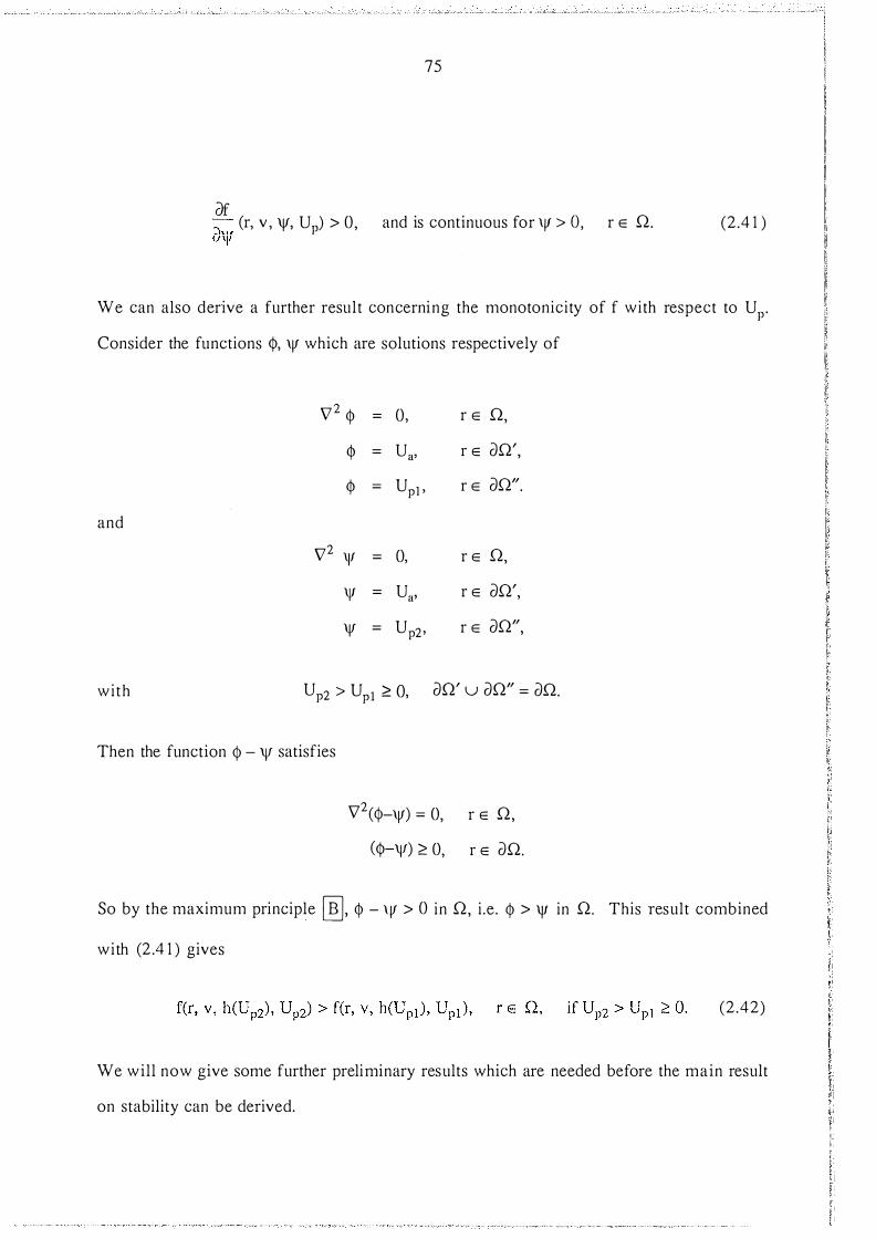
75

df ;-- (r, v , \jf, Up) > 0, and is continuous for 'V > 0, r E n. o\V (2.4 1 )

We can also derive a further resul t concerning the monotonicity of f with respect to UP.

Consider the functions <j>, \jf which are solutions respectively of

\72 <1> = 0, r E n,

 = Ua, r E an',

 = url ' r E an".

and

\72 'I' = 0, r E n,

'" = Ua, r E an',

\jf = ur2' r E an",

with ur2 > ur1 :::: o, an' u an" = an.

Then the function <j> - \jf satisfies

V2(<j>-\jf) = 0, r E n,

( <j>-\jf) :2: 0, r E an.

So by the maximum principle �' <1> - \jf > 0 in n, i .e. <1> > 'I' in n. This result combined

with (2.4 1 ) gives

(2 .42)

We wil l now give some further preliminary results which are needed before the main result

on stability can be derived.

76

Theorem 2.2.5

Let F(r, cp, h, Up) satisfy

F(r, cp, h , Up) > f(r, \jf, h , Up) , on Q, if cp > \Jf � 0, and suppose for some UP > 0 a positive solution cp(r, UP) exists for the problem

cp = 0, r E CJQ.

Then the minimal positive solution V (r, Up) of (2.37) satisfies

Proof

Similar to proof of Theorem 3.3 , Keller and Cohen [37] p 1 367.

Corollary 2.2 .6

The minimal solution V (r, Up) of (2.37) is an increasing function of UP, on 0 < UP < Up, crit·

Proof

For any fixed value of UP in the interval 0 < UP < u; < Up, crit' define

F(r, V , h, Up) = f(r, V , h, u;) .

Then for this value of UP , the hypothesis of Theorem 2 .2 .5 is satisfied , say with

cp(r , Up) = V(r, u;) .

So by Theorem 2.2.5,

Also

and

77

< 0 , r E n, by (2.42),

V (r, u;) - V(r, Up) = 0, r E an.

So by the maximum principle �, V(r, u;) > V(r, Up) i n n. This completes the proof.

It i s well-known (see e . g. Diekmann and Temme [ 43] p48) that the occurrence of

criticali ty ( i .e . UP = Up, crit) corresponds to the existence of a non-trivial solution of the

l inearized version of the system (2 .37) . In fact this result i s just the contra-positive of the

implicit function theorem. With this in mind, a mathematical defin ition of Up, crit i s that i t i s

the smallest value of UP such that the system

exp --( -1 ) V + h

V211r + 'l1 1 1r = 0 n '�' , I (V + h)2 '�'

, r E � '- ,

'V = O , r e an,

(2 .43)

h as a non-trivial solution, where V i s the minimal solution of (2.37) . That i s Up, crit is the

smallest v alue of UP such that 111 (Up) = 1 , where 111 (Up) is the principle eigenvalue of

Theorem 2.2.7

78

\jf = 0 r E on.

(2 .44)

Let UP lie in the open interval 0 < UP < Up, crit· Then each UP in this interval must satisfy

1 < )l1 (Up) where )l1 (Up) is the principle eigenvalue of (2.44) .

Proof

As mentioned by Keller and Cohen [37] in the proof of Theorem 4. 1 p 1 370, the function

exists and is continuous in UP on 0 < UP < Up, crit (see note below). The function m then

s at i sfies

2 ()f ()f ()h V m + 11 ()v (r, V, h , Up)m = - 11 ()h (r, V, h, Up) ()Up'

m = () , r E on.

r E n, ) (2 .45)

Now (2 . 40) , (2 . 4 1 ) give ()f av > O, ()f

()h > 0 respectivel y , and the function

r E n

n(on') = 0,

n (on") = 1 , an' u an" = an,

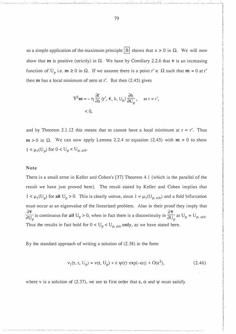
79

so a simple application of the maximum principle [0 shows that n > 0 in Q. We will now

show that m is positive (strictly) in Q. We have by Corollary 2.2.6 that V is an increasing

function of UP i.e. m ;:::: 0 in Q. If we assume there is a poin t r' E Q such that m = 0 at r'

then m has a local minimum of zero at r'. But then (2.45) gives

< 0,

and by Theorem 2. 1 . 1 2 this means that m cannot have a local minimum at r = r'. Thus

m > 0 in Q. We can now app ly Lemma 2.2.4 to equation (2.45) with m > 0 to show

1 < Il l (Up) for 0 < UP < Up, criv

Note

There i s a small error i n Keller and Cohen's [37] Theorem 4. 1 (which i s the paral lel o f the

result we have j ust proved here) . The result s tated by Keller and Cohen impl ies that

1 < Ill (Up) for all UP > 0. This is clearly untrue, since 1 = Il l (Up, crit) and a fold bifurcation

must occur at an eigenvalue of the linearized problem. Also in their proof they imply that av av au is continuous for a l l up > 0, when in fact there is a discontinuity in au at up = up, cril" p p Thus the results in fact hold for 0 < UP < Up, crit only, as we have stated here.

B y the standard approach of writing a solution of (2.38) in the form

where v is a solu tion of (2.37), we see to first order that E, a and 'I' must satisfy

(2 .46)

80

(2 .47)

\lf = O , r E on.

So by (2.46) a solution is stable under a small perturbation if the principle eigenvalue, a1 ,

of (2.47 ) i s positive and unstable if a1 i s negative.

These results can be combined to give the following result concerning stabi lity.

Theorem 2.2.8

For 0 < UP < Up, crit> the minimal positive solution v (r, Up) of the problem (2 .37) is stable.

Proof

This is similar to that given i n Keller and Cohen [37 ] , but we will g ive the detai l s here for

completeness. Let V (UP, r) be the minimal positive solu tion of (2.37) , and let a1 (Up) be

the principle eigenvalue of (2.47) , then the variational characterization of a1 (Up) gives

where Q is the set of admissible functions, i .e.

Q ={ <j>(r) : <j>(r) > 0 on n, <j>(r) E C(Q) n C1(n) , <j> (r) = () on an} .

(2 .48)

We can al so write, by the variational characterization of the principle eigenvalue of the

problem (2.44) ,

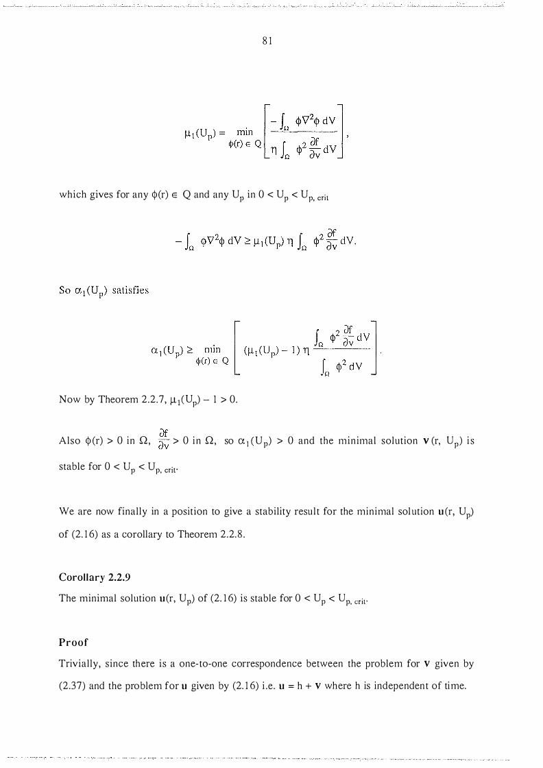
8 1

which gives for any <j>(r) E Q and any Up in 0 < Up < Up, crit

Now by Theorem 2.2.7, jl1(Up) - 1 > 0.

Also <j> (r) > 0 in Q, g� > 0 i n Q, so cx. 1 (Up) > 0 and the min imal solution V (r, Up) i s

stable for 0 < up < up, crit"

We are now finally in a position to give a stability resul t for the minimal solution u (r, Up)

of (2. 1 6) as a corollary to Theorem 2.2. 8 .

Corollary 2.2.9

The minimal solution u (r, Up) of (2. 1 6) is stable for 0 < UP < Up. criv

Proof

Trivially, since there is a one-to-one correspondence between the problem for V given by

(2.37) and the problem for u given by (2. 1 6) i .e. u = h + V where h is independent of time.

82

2.2.12 Comparison of critical press temperatures

A comparison of the critical press temperatures (in degrees Celsius) as a function of the

dust l ayer height for the three methods is given in Figure 2. 1 3 below.

....-;-13 bb � � ...... 0 0. 8 � ] 0

280

2.70

260 2!10 240 230

220

210

200

190

180 0 10 20 30 -10 50

Height of Fibre/Oil Layer (cm)

GO

LEGEND

a ruU 3·u uumnin, full Anhcnius ICIIII

a luflnilc slab npp1u�. full Arrhcnlus 1c1m

u lufiuilc slab npprox, Prnuk-KaJilCIICL�kii apprw,.

70

Figure 2.13 Graph of the height of the fibre/oil dust layer against the critical

temperature of the press for the three models d iscussed in this Chapter.

2.2.12.1 Advice to the company

On the basis of the model which best approximates the physical situation , i .e . the Full

Arrhenius term with ful l three dimensional domain model , spontaneous ignition of the

fibre/oil layer will be likely when both the dust layer exceeds 20cm in height and the press

temperature rises above 220°C. The company, therefore, should be advised to adj ust their

cleaning procedures accordingly and also to monitor the press temperatures .

83

2.2.12.2 Infinite slab approximation to the domain

As would be expected, for a11 < l Ocm the domain approximates well to an infinite slab.

However, for a11 > l Ocm (the practical range of i nterest) the approximation becomes

i ncreasingl y poor, with up to a 1 5% difference in the critical press temperatures for the

range of ah considered .

2.2.12.3 On the Frank-Kamenetski i a pproximation

For the range of dust l ayers and press temperatures considered , the Frank-Kamenetskii

approximation seems to perform well in the infinite slab domain . However, it should be

observed that even though we have retained the ful l Arrhenius term, the resu l ts for the

infinite s lab model are not independent of the Frank-Kamenetskii approximation . This is

because the method outlined in Chapter 1 was used to derive the activation energy of the

reaction and the physical constants for the model, and this uses the Frank-Kamenetskii

approximation. So we are really comparing how the two equations in the infin ite slab

domain behave with the same physical constants . The true validity of the Frank

Kamenetskii approximation can therefore only be determined when an experimen tal

method for the derivation of the relevant physical constants is developed that does not

itself use the approximation.

2.2.12.2 Comment on plots as a 11 --7 oo

O n physical grounds , i t is expected that the graph corresponding to the ful l three

dimensional domain model should have a horizontal asymptote as a11 --7 oo, i.e. the critical

temperature for the corresponding semi-infinite rod . For the models that use the infinite

slab domain approximation , the whole upper half plane is fi l led as a11 --7 oo , thus it is

expected that Tp. crit --7 0 as a11 --7 oo for these models.

84

2.2.12.3 Multi p l icity of steady states

The occurrence of a series of 'intermediate' s teady state solutions (Figure 2. 1 1 ) is only

observed for the ful l three dimensional domain model . For the symmetrical heating case

gross multiplicity of steady state solutions was first observed by S teggerda [ 44] i n the

unit sphere, and does not occur in the infinite slab. These observations suggest gross

multiplicity of steady state solutions is a property of three dimensional regions i n contrast

wi th the situation for 'one dimensional ' domains . Thi s conjec ture requires further

investigation but is not of special relevance to the practical concerns of th is Chapter.

85

CHAPTER 3

Thermodynamic derivation of a model for the self-heating o f damp

cellulosic materials

3.1 Heat producing reactions

Since this work was motivated by the study of bagasse, a material that goes through a

refining process before storage, we shall ignore heat produced by the metabolism of living

cel l s from freshly harvested materials . The chemical reactions outl ined schematical ly

below are likely to hold for most self-heating damp cellulosic bodies.

( i ) CELLULOSE + OXYGEN � PRODUCTS + HEAT,

an exothermic oxidation reaction.

(ii) CELLULOSE + WATER + OXYGEN � PRODUCTS + HEAT,

an exothermic hydrolysis reaction.

(iii) MICROBES + SUGARS + WATER + OXYGEN � PRODUCTS + HEAT,

metabolism of bacteria and fungi, an exothermic process, ( 'sugars' would inc lude

glucose).

( iv ) WATER VAPOUR � LIQUID WATER,

an exothermic condensation process.

( v ) LIQUID WATER � WATER VAPOUR,

an endothermic evaporation process .

On the basis of the experimental work done on bagasse by Dixon ] 23] outlined i n Chapter

1 , we shal l neglect the heat produced by (iii), i .e. by the action of microbes, in this thesis.

86

3.2 Assumptions

In the derivation of the mathematical model we shall make the following assumptions

( i ) That reactant consumption, or the formation of reaction products, does not effect the

rates of any of the reactions in the system. Thi s is a parallel assumptio n to that

made by the classical model for the self-heati ng of a body by a single exo thermic

reaction .

( i i ) That there is no forced convection through the system. Th i s 1 s a reasonable

assumption provided there i s no applied pressure grad ient.

( i i i ) That the thermal conductivity coefficient and the coefficient of diffusivity of water

vapour through the system are constant.

( i v ) That the dry air/water vapour mixture behaves a s an ideal gas.

( v ) That heat can trave l through the system b y conduction and also by the diffusion of

water vapour. Liquid water remains static in the system unti l vaporized.

(v i ) Heat i s lost a t the boundary by Newtonian cooling. No moisture i s transferred

across the boundary - th i s assumption i s based on Dixon 's [23 J comments on

bagasse, and i s l ikely to be val id for other cel l ulosic substances, espec ia l ly those

stored under a cover.

(v i i ) As a resu l t of assumptions ( i ) and (vi) , total moisture content in the system is

conserved .

(vi i i ) Dry air concentration i s constant in the body.

87

In our formulation of the equations we shall also include the effects of natural convection in

the system for the sake of completeness. In our analysis of the resul ting formulation

however, we shal l , for the same reasons outlined by Henry [25] in Chapter 1 , ignore these

convection effects.

3.3 Derivation of the equations

3.3.1 Conservat ion law

In the derivation of this model we will use the conservation equations for energy and

mass. We will first derive the basic conservation equation we will be applying ( see for 1\ 1\

example Aris [45] p50). Consider a quantity inside a closed region Q with boundary an.

L . . 1\ 1\ 1\ Q/\ 1\

0 . 1\ 1\ 1\

Q/1. I\ et the quanti ty have concentration A(r , t ) , r E , t > , and flux j ( r , t ) , r E , t > 0,

where j is a vector such that the amount of the quantity per unit area per unit time that

crosses an element with normal !!. is j . !!.·

1\ I\ I\ I\ I\ I\ Also let g(r , t ) , r E Q, t > 0 represent the rate of generation of the quantity in Q. We

wil l assume that A , j and g are conti nuous functions of � . If we now consider a region D 1\

where D c Q, with boundary ao, and outward normal on the boundary !!_ , then the rate of

change of the amount of the quantity in D is

a f I\ 11. A dV , a t D

the rate at which the quantity crosses an i s

I I\

j . n dS , JD

and the rate of generation of the quanti ty within D is

I I\ g ci Y . D

88

Now by Green's theorem we can write

I 1\ I 1\ j . n dS = V' . j dV ,

()!) � � I)

so we can balance the three terms to give the conservation equation for the quantity as

J ( a� + v . j - g J dV = o . D d t �

1\ Since this equation must hold for any region D c Q, we have

i1A . 1\ 1\ + V' . J = g, in Q, d t

as the basic conservation equation for any quantity in the region .

3.3.2 Enthalpy per unit volume of the body

( 3 . 1 )

Assuming the body consists of cel lulosic solid, liquid water, water vapour, and dry air,

then the following expressions are obtained for the enthalpy per unit volume of each of the

constituent components of the body

enthalpy of cel lulosic solid = Hs,

enthalpy of liquid water = XHW,

enthalpy of water vapour = YHV,

enthalpy of dry air = PaHa.

where

= enthalpy of the cellulosic solid per tA�·�� vol 1Ari1e,

= partial molar enthalpy of liquid water,

89

Hv = partial molar enthalpy of water vapour = Hw + Lv, LV = latent molar heat of vaporization of liquid water,

Ha = partial molar enthalpy of dry air,

X = l iquid water concentration per unit volume,

y = water vapour concentration per unit volume,

Pa = dry air concentration per unit volume.

Thi s gives the enthalpy per unit volume of the body as

1\ Differentiation of (3 .2) with respect to t gives

(3 .2)

We wi l l assume Hw , Hv, Ha, H5 are functions of T only . I n fact if we are deal ing with an

ideal gas we lose noth ing by this assumption. General ly the Hi , i = I , . . . , 4, ti = (I-lw , Hv ,

Ha, H5) will also be functions of X, Y, p (where p = pressure), for example

However, if we assume the dry air/water vapour mixture i s an ideal gas, then the last term d i-l · d i-l ·

vanishes . Also as Aris [451 observes, the sum of the contri but ions of the ax1 , () y1 , ()Eh . i = 1 , . . . , 4 terms to the -r;: expressiOn i s zero s ince the Hi , i = 1 , . . . , 4 are in tensive d t

thermodynamic properties.

90

This gives

( 3 . 3 )

where the coefficient o f a; is the specific heat per unit volume of the system and wil l be a t

written as C5•

That i s

giving

oE11 = C oT + oX I-I oY A s A A w + --;- Hv .

a't' a't' a't' a't'

3.3.3 Transport of heat and mass in the system

(3 .4 )

Heat and mass wi l l be transported in the cel lu lose/liquid water/water vapour/dry air

mixture by several means

( i ) Conduction o f heat due to temperature differences i n the system.

(ii) Diffusion of water vapour due to concentration differences in the system.

(iii) Convection of water vapour through the system. In the absence of forced

convection, this will be by natural convection arising from differences in the average

density of the water vapour/dry air mixture.

9 1

The enthalpy flux fe wil l include contributions from each of the above three factors. I n fact

we can write

( 3 . 5 )

where fc i s the contribution to the enthalpy fl ux by conduction of heat and fv 1 s the mass

flux due to the diffusion and convection of water vapour.

Mass flux

In the system we are considering, the only movement of mass is that associated with the

diffusion and convection of water vapour. An important variable for describing convective

effects in porous systems is the volume flux, also known as the superficial velocity, y. We

will assume that this volume flux satisfies Darcy's law i.e.

K V = -- (\7 p - (p a + Y) g ) , � !l �

( 3 . 6 )

where p i s the pressure, K i s the permeabil i ty of the system, ).l is the viscosity of the

water vapour/dry air mixture and the vector g represents grav itational effects. A ssuming

the water vapour/dry air mixture behaves as an ideal gas the pressure p is given by

( Y Pa ) p = RT M ! + M2 , ( 3 . 7 )

where M1 i s the molecular weight of water vapour and M2 i s the molecular weight of dry

air. The mass flux can then be written as

F = -DVY + Yv ,...., V ......., ' ( 3 . 8 )

where -DVY i s the contribution of diffusion o f the water vapour and D i s the diffusivity of

water vapour in the system.

92

Enthalpy flux

Assuming the contribution of conduction of heat to the overal l enthalpy flux is given by

F = -k'VT � C ' ( 3 .9)

where k i s the thermal conductivity of cel lu lose, we can combine equation s (3 .5 ) and (3 .8)

to give the total enthalpy flux as

fc = -k'VT + Hv f -D'VY + Yy ] .

3.3.4 Rates of generation of hea t and mass in the system

( 3 . 1 0)

We wil l assume there are two exothermic chemical reactions occurring in the system, the

classical oxidation reaction and an anci l lary hydrolysis reaction due to the presence of

water. We wil l further assume that the rate of the oxidation reaction is given by the

Arrhenius law, so

where

rate of heat production by the oxidation reaction = QpZ exp ( �� ) , Q = exothermicity per uni t volume of the oxidation reaction,

Z = pre-exponential factor for the oxidation reaction,

E = activation energy of the oxidation reaction ,

p = cell ulose concentration per unit volume.

(3 . 1 1 )

For the hydrolysis reaction we wil l fol low Gray !30] in assuming that this reaction i s first

order in the liquid water and cellulose concentrations, and that the reaction rate obeys the

Arrhenius law, i .e .

93

rate of heat production by the hydrolysis reaction = QwPZwX exp (-:T } (3 . 1 2)

where

Qw = exothermicity per unit volume of the hydrolysis reaction,

Zw = pre-exponential factor for the hydrolysis reaction,

Ew = activation energy of the hydrolysis reaction .

A lthough moisture can change between the liquid and vapour phases in the system, there

is no net production or consumption of moisture in the body. Simi larly there are no

changes in the cellu lose or air concentrations , so the rate of generation of mass in the

system is zero.

3.3.5 The mass conservat ion equation

Applying the basic conservation equation (3 . 1 ) to the mass balance problem in the region 1\ Q , with mass flux given by (3 .8 ) gives

acx + Y) " " " " + \7 . { -D\?Y + Tv } = 0 , r E Q , t > 0.

a t � (3 . 1 3 )

Given that liquid water remains static in a unit volume of the body, the rate equation for

the change in liquid water concentration in un it volume is given by

ax rate of water vapour --;;: = condensation a t

Following Gray [30] , we wil l assume:

rate of liquid water evaporation

( i ) t ha t the rate of the (exothermic) condensation reaction is independent of

temperature and is first order with water vapour concentration,

94

(i i ) that the evaporation of water is the rate determining step in transfer to the vapour

phase, and that this is an endothermic reaction with an activation energy equal to

the latent heat of vapourization of liquid water, and is first order with l iquid water

concentration.

This gives, again assuming Arrhen ius kinetics,

rate of water vapour condensation = Zc Y ,

rate o f liquid water evaporation = ZcX exp ( ��) where

Zc = constan t of proportional ity for the condensation process (equivalent

to a pre-exponential factor) ,

Zc = pre-exponential factor for the evaporation process.

So we have the fol lowing rate equation for X

1\ t > 0.

Substi tuting this expression in (3 . 1 3) gives the rate equation for Y as

()y ( -Lv ) 1\ 1\ 1\ at' = zcx exp RT - zc y - V' . { -DV'Y + Yy_ } ' r E .Q, t > 0 .

(3 . 1 4)

(3 . 1 5 )

95

3.3.6 The energy conservation equation

Applying (3 . 1 ) to the energy conservation equation with enthalpy flux given by (3 . 1 0) and

the rate of generation of heat given by (3 . 1 1 ) and (3. 1 2) gives

en ax aY C5 t: + t:: hw + f\ hv + V . { -kVT + Hv [ -DVY + Yv ] } d t d t Cl t �

( -E ) ( -Ew ) 1\ 1\ 1\ = QpZ exp RT + QwPZwX exp RT , r E Q, t > 0,

(as Hv = Hw + Lv and by (3 . 1 3) , (3 . 1 4))

1\ 1\ r E Q, 1\ t > 0. ( 3 . 1 6)

The term -DVY . VI-Iv is usually neglected in models of thi s nature. As Aris [45] states

" [this] term seldom appears in any derivation of such an equation and when it does

appear is usually neglected without more ado. Amundson 1 4 6 1 has incl uded it in

his discussion of models of the fixed-bed reactor, but remarks that he knows no

experimental or theoretical work that has been done to justify this neglect . . . We

also bow down in the house of Rimmon and sacrifice it to the demands of

simplicity. "

In his work on the coupled diffusion of heat and moisture i n bulk wool , Heath [47] has stated that this term is small in comparison with V . (kVT), with the ratio of order

1 o-2 6 Y. In this thesis we will follow the lead of Aris and Heath and neglect the

-DVY . VHv term.

3.3.7 Boundary and in itial conditions

96

As mentioned in section 3.2 we shal l assume the temperature change across the boundary A A

a n i s governed by Newtonian cooli ng and that no moisture crosses an. This gives

where h is the heat transfer coefficient between the body and i ts surroundings,

ay - 0 an - '

ax -= 0 an '

A r E

A r E

A an,

A t > 0 ,

A an,

A t > 0.

(3 . 1 7 )

(3 . 1 8 )

(3 . 1 9)

We shal l also take the variables T6, �) , Y(�, t\ X(�, �) to have the initial profi les

A A , A A A T(r , t = 0) = r l (r ) � 0, r E Q

A A A A A Y (r, t = 0) = Y1 ( r ) � O, r E Q

A A A A A X(r , t = 0) = X 1 ( r ) � 0, r E Q.

3.3.8 Model equations with and without convection

Now

(3 .20)

(3 .2 1 )

(3 . 22)

97

where the standard state of water is liquid at temperature T0, and Cw is the specific heat

of liquid water. So

(3 . 23)

Then assuming k and D are constants, the reaction/diffusion/convection system for the seven variables T, Y, X, �, p i s

1\ 1\ 1\ r E Q, t > 0,

ay (-Lv) ? 1\ 1\ 1\ a� = Z

cX exp RT - Zc Y + D\7-Y - Y\7 . � - � . \7Y, r E Q, t > 0 ,

ax (-Lv) " " " a� = Zc y - zcx exp RT '

r E Q, t > 0,

K 1\ 1\ 1\ V = - - (\7p - (p + Y)g) , r E Q, t > 0, � ll

a �

( Y Pa ) 1\ " 1\ p = RT - + - , r E Q, t > 0, M l M2

with the boundary conditions (3 . 17) - (3 . 1 9) and ini tial conditions (3 .20) - (3 .22).

98

Neglecting natural convection, i.e . setting v = 0, the reaction/diffusion system for the three � �

variables T, Y, X becomes

()T (-E ) (-Ew) CS a1 = QpZ exp RT + QwP ZwX exp RT

11 11 11 r E £2, t > 0, (3 .24 )

(3 .25)

(3 .26)

with the boundary conditions (3 . 17) - (3 . 1 9) and the initial conditions (3 .20) - (3 .22) . For

the reasons outlined earlier in this Chapter and in Chapter 1 i t i s the solution of the

reaction/d i ffus ion sys tem (3 .23) - (3.25) that we sha l l consider for the rest of t h i s thes is .

3.4 Dimensionless formulation of the equations

3.4.1 Dimensionless formulation of the spatially distri buted equations

S e t

RT u = - , E

E w L V a = - , E

O:. w = - , E

J6 (Y1 (r) + X1 (r))crv /.. =

>

11'

r r = - , ao

zc QC ::= -, z

Ylp kE

pQRZa� '

YV1 y = A ) Jn (YI (f) + xl uwv

RpQZt t = --'-

CSE >

RpQ E = --

(' E'

's L V h = -c ' Q

D

y = - , a ' z

0

pz Q w == -w '

z

(3 .27)

99

A A A where V 1 is the volume of the region n. Also let n and an be mapped into n and an

respectively by the transformation r = �/a0 . Here A is a constant which represents the

ratio of total moisture concentration to cel lulose concentration in the body. Then the non-

d imensioned representation of the equations (3 .24) - (3 .26) i s

au (- 1 ) { (-awJ (-aJ } at = exp � + A hw <Pw X exp -u- - he <Pc X exp --;- + he <Pc Y

� (-aJ 2 £ O t = <Pe X exp � - <Pc y + y \1 y,

ax (-aJ E at = <Pc y -<Pe x exp -t� ,

Also setting

ha0 B i = -

k

r E n,

r E n, t > 0,

t > 0.

( 3 .28 )

(3 .29)

( 3 . 30)

(3 . 3 1 )

the non-dimensioned version s of the boundary conditions (3 . 1 7) - (3 . 1 9) and the in i tial

conditions (3 .20) - (3 .22) are, respectively ,

au . � + B I (ll - U ) = 0, r E an, t > 0, on

� - 0 :"I ll 0 On - , r E Ul:.l., t > ,

ox Ol1 = 0, r E on, t > 0,

MASSEY U NIVERSin llBRAR.'i

( 3 . 32)

(3 . 3 3 )

(3 . 34)

and

100

u (r, t=O) = �1 (r) ?:: 0, r E Q,

y(r, t=O) = \jf 1 (r) ?:: 0, r E Q,

x(r, t=O) = X ! (r) ?:: 0 , r E Q.

3.4.2 Dimension less fommlati on of the spatia l ly uniform case

( 3 . 35 )

( 3 . 36)

(3 . 37)

By the 'spatia l ly uniform case' we mean the limiting case of the equations (3 . 1 7 ) - (3.26)

as k --7 oo and D --7 oo . As k --7 oo and D --7 oo , equations (3 . 1 7 ) - (3 .26) wil l only be aT satisfied if 'V2T --7 0, 'V2Y --7 0 and ::;- --7 0. So in the limit k --7 oo , D --7 oo the state un

variables T, Y and X wil l be independent of the space variable � - Integrating (3 .24) across 1\

the region Q and applying Gauss' s theorem gives

a (f /\ ) f (-E\i/\ f (-Ew�/\ CS a� 6. T dV = Qp z {l exp RT r V + QwPZw 6. X exp RT t V

In the limit k --7 oo, D --7 oo we thus obtain

dT (-E) (-Ew) V 1 Cs d1 = QpZV1 exp RT + QwPZw V1X exp RT

1\ t > 0,

where T = T(�) , Y = Y(�) and X = X(�), and S is the surface area or the region £1.

(3 . 3 8 )

1 0 1

Similarly for (3 .25) , (3.26) we obtain

1\ t > 0, (3 .39 )

1\ t > 0. (3 .40)

The init ial conditions (3 .20) - (3 .22) become

1\ T( t =O) = T1 , (3 .4 1 )

1\ Y ( t=0) = Y 1 , (3 .42)

1\ X( t =O) = X1 . (3 .43 )

As total moisture conten t is conserved in the system, we can eliminate Y from the above

equations (3.38) - (3 .43) . By adding (3.39) , (3.40) we see

which implies

that is

d (X+Y) 1\ 1\ = 0, t > 0, d t

1\ 1\ 1\ Y ( t ) + X( t ) = Y1 + X1 , for all t > 0,

1\ 1\ 1\ Y ( t ) = Y 1 + X 1 - X( t ) , for all t > 0.

1 02

We can then eliminate Y from our equations to give

(3 .44)

( 3 .45)

with the ini tial conditions (3 .41 ) , (3 .43).

Where applicable, the non-dimensionalization of these equations is similar to that used in

(3 .27) , (3 . 3 1 ) except

X x = x + Y ' 1 1

This gives the final non-dimensional form of the spatially uniform case as

du (- 1 ) { (-a ) (-a) dt = exp -;- - L(u-U) + A-1 hw<Pwx exp � - hc<Pex exp �

dx (-a) E dt = <Pc( l-x) - <Pex exp � , t > 0 ,

(3 .46)

(3 .47 )

( 3 .48 )

with the initial conditions

1 03

u(t=O) = s 1 ,

x(t=O) = X1 •

3.5 The steady state equations for the spatia l ly distr·ibuted model

(3 .49)

(3 .50)

Our conservation of total moisture content assumption also means that at steady state

solutions of (3.28) - (3 .37) , that is where

du � dx d t = d t = d t = O,

we can eliminate both y and x from the equations to give a single equation in u only.

Adding (3 .29), (3 .30) and integrating across the region .Q gives

= y J Vy . n c!S , an - by Gauss 's theorem

S o

= 0, as �y_ = () r E dfl. dn '

Jn (x+y) c!V = Jn (\jf1 +X1 ) c!V = V, for all t > 0,

where V is the dimension less volume of the region Q (= V 1 I a5) .

( 3 . 5 1 )

1 04

The steady state equations for the spatially distributed model are

. . . . . (3 .52)

r E .Q,

<PcY - <Pcx exp(-l�) = 0, r E .0.,

where 11 = -1 , with the boundary conditions (3 .32) - (3 . 34). 11'

Now adding (3 .53) , (3 .54) shows that the steady state solution for y must satisfy

� = () r E a.Q, an '

which implies that y must be a constant in .Q at steady state. In fact, using (3 .5 1 )

y = 1 - � Jn x dV,

and by (3 . 54)

<Pc ('aJ x = <Pc y exp ; ,

( 3 . 53 )

( 3 . 54)

(3 . 55 )

( 3 .56)

105

s o <Pc J (aJ y = 1 -- y exp - dV, <Pc V n U

at steady state. y = <Pc J (aJ <Pc + y n exp -;:;- dV

Finally substituting for x and y in (3 .52) gives the steady state equation for u as

\7 u + 11 exp --;:;-- + <Pc a exp -L-I - = 0, 2 [ (-1 ) Ahw<Pw<Pc (a-awJ] <Pc +y Jn exp(-;:;-J dv with the boundary condition (3. 32) i .e.

�u + Bi (u-U) = 0, r E ()Q. on

r E Q,

( 3 . 57)

( 3 . 58 )

The spatially uniform model

4.1 Introduction

1 06

CHAPTER 4

The coupled pair of non-linear ordinary differen tial equations, i.e. (3 .47), (3.48), we will be

studying in this Chapter are of the form

where

du dt = f(u, x, Q, �), t > 0,

dx dt = g(u, x, Q, �), t > 0,

Q = (U , L, A1 ) ,

(4 . 1 )

(4 .2)

We have spli t the parameters of the system up into two groups, those in Q and those in �·

In a set of experiments to be carried ou t on a particu lar self-heating substance , the

parameters that can be varied are : T a the ambient temperature , � 1 the surface area to

volume ratio of the sample, and X 1 + Y1 , the total initial moisture content . Thus the vec tor

Q contains 'variable' parameters - parameters that can be varied while analysing a particular material . However Q, Qw, C5, p, Z, Zw, E, Ew etc. are 'constant ' parameters in that they stay fixed for a particular material . We have grouped these 'con s tant '

parameters in the vector ..§ . So in effect we are deal i ng with a two variable, three parameter problem.

To obtain a complete description of all the qualitatively distinct behaviour of the system,

we must analyse the fu ll parameter space of each of the componen ts of o . To do this we wil l use the method of degenerate singularity theory which is outl i ned in detai l i n

Golubitsky and Schaeffer [48]. Degenerate singu larity theory provides a means of fi nding

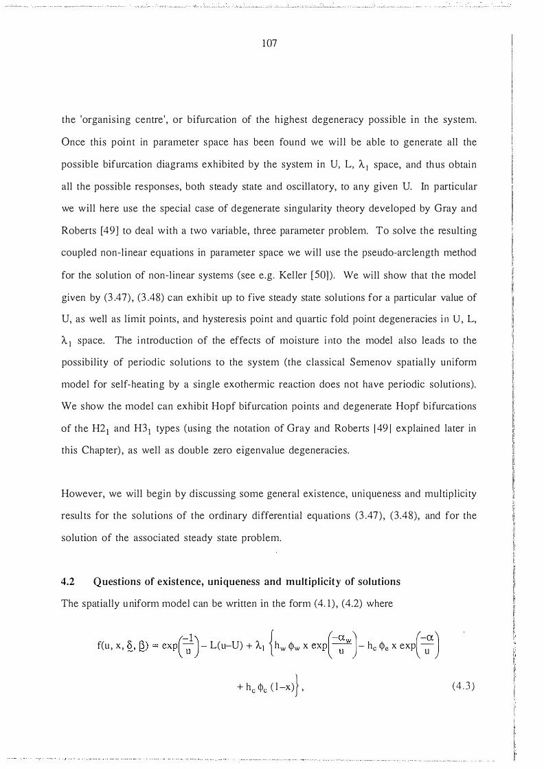
107

the 'organising centre' , or bifurcation of the highest degeneracy possible in the system.

Once this poin t in parameter space has been found we wil l be able to generate all the

possible bifurcation diagrams exhibited by the system in U, L, A 1 space, and thus obtain

all the possible responses, both steady state and oscillatory, to any given U. In particular

we will here use the special case of degenerate singularity theory developed by Gray and

Roberts [ 49) to deal with a two variable, three parameter problem. To solve the result ing

coupled non-linear equations in parameter space we will use the pseudo-arclength method

for the solution of non-linear systems (see e.g. Keller [501 ) . We will show that the model

given by (3 .47) , (3 .48) can exh ibi t up to five steady state solutions for a particular value of U, as well as limit poin ts , and hysteresis point and quartic fold point degeneracies i n U , L,

A 1 space. The i n troduction of the effects of moisture i nto the model also leads to the

possibility of period ic solutions to the system (the classical Semenov spatially uniform

model for self-heating by a single exothermic reaction does not have periodic solutions).

We show the model can exhibit Hopf bifurcation points and degenerate Hopf bifurcations

of the H21 and H31 types (using the notation of Gray and Roberts 1 49 ] explained later in

this Chap ter) , as well as double zero eigenvalue degeneracies.

However, we will begin by discussing some general existence, uniqueness and multipl ici ty

resul ts for the solutions of the ordinary differen tial equations (3 .47 ) , (3 .48), and for the

solu tion of the associated steady state problem.

4.2 Questions of existence, uniqueness and multipl icity of solutions

The spatially uniform model can be written in the form (4. 1 ) , (4.2) where

f(u , x, £ , �) � ex{�) - L(u-U) + >.1 { hw $w x exp(-�w )- h, $, x ex{,� J + hc <Pc ( l -x)} , (4 . 3 )

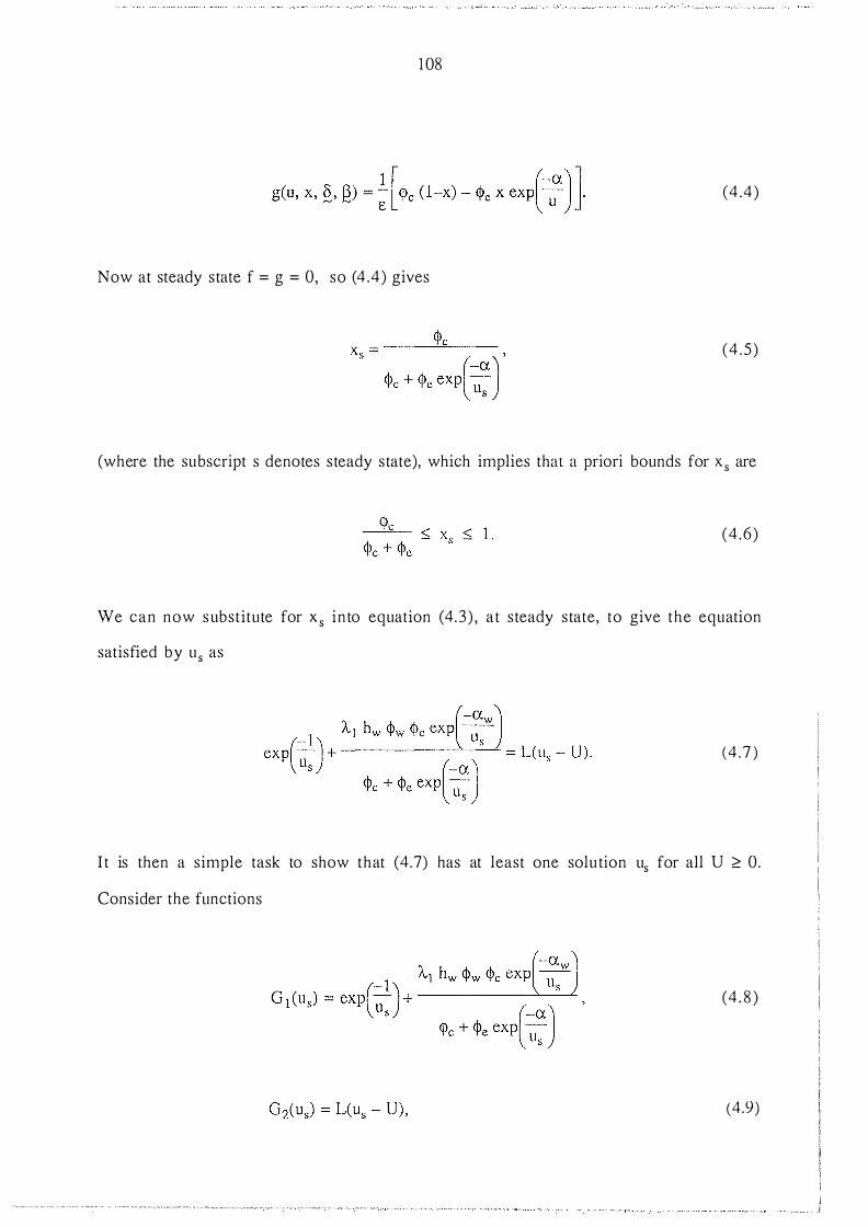
1 08

(4 .4)

Now at steady state f = g = 0, so ( 4 .4) gives

(4 .5 )

(where the subscript s denotes steady state), which implies that a priori bounds for x5 are

(4 .6 )

We can now substitute for x5 in to equation (4. 3 ) , a t steady state, to give the equation

satisfied by u5 as

( 4 .7 )

I t is then a simple task to show that (4.7) has at least one solu tion u5 for all U 2 0.

Consider the functions

(4. 8 )

(4.9)

109

for any fixed U ::::: 0, where 0 1 ( us ) represents the rate of heat release by the various

reactions at s teady state, and G2( us) the rate of loss of heat due to Newtonian cooling.

Now G 1 (0) = 0 , G2 (0) = -LU (so c learly U = 0 has the solution u s = 0), G 1 ( oo ) is

positively finite (in fact it equals 1 + (A. 1 hw <Pw <Pc I C<l>e + c)), and G2( oo) is positively

infinite. So by the intermediate value theorem there must be at least one value us = us * ,

In showing that the system can exhibit five steady state solutions for a certain p arameter

range we will use a similar graphical approach to that of Gray [30] . Figure 4 . 1 below

shows an example set of us , 01 ( us) curves as the dimensionless initial moisture content

A.1 increases (with a > aw) ·

AI increasing '

Us

Figure 4. 1 Rate of heat release curves as A.1 increases from zero

1 10

We can see that for A1 sufficien tly large, the heat release rate curve can have a negative

slope. Thus, as the function G2(u5) is a straight line, for this parameter range ( 4.7) can

have up to five solutions . It is simple to deduce that a necessary condition for this

negative slope to appear is that the second term in (4.8) has a maximum. Thi s in turn can occur if a > aw. So a > aw i s a necessary but not sufficient condition for our system to

have five steady state solutions. Figure 4.2 below shows some example U , u5 steady

state bifurcation diagrams, as A t i ncreases, for the case a > aw.

A,1 increasing u

u

Figure 4.2 Example bifurcation diagrams, as At increases, for a > aw

We observe that as A1 (the dimensionless characterization of the total moisture content in

the body) increases the ' traditional' critical ambient temperatures, corresponding to the first limi t point on the A t = 0 curve, decreases. For A 1 = A t ' the d iagram has four l imi t

1 1 1

points and an intermediate steady state is reached as U increases past the firs t limit point . It is interes ting to note that for A-1 sufficiently large, eg A-1 = A,{, the lower right

hand limit point is to the right of the higher right hand limit point, so this lower limit point

now defines the Ucrit value for the system. These diagrams show how Ucrit can be

substantially reduced by the inclusion of the effects of moisture content in the model. This

may explain the comments in Figure 1 .9 of Chapter 1 .

A well-known (see e.g. Ray [5 1 ] ) condition for (4. 1 ) , (4.2) to have a unique, stable steady

state solution for all U � 0 is

Det (J ) > 0, (4 . 1 0)

Tr (J) < 0. ( 4 . 1 1 )

Here Det (J) is the determinant of the Jacobian matrix of the system ( 4. 1 ) , ( 4.2) evaluated at the steady state u5 , X5 ,

df df

J = [ J l l J1 2 J = du dx

J21 J22 � � du dx u = us

X = X5

and Tr (J) is the trace of this Jacobian.

So

and

Det J _ df � df � ( ) - du dx - dx du , evaluated at u5, x5,

df � Tr (J) = du + dx , evaluated at u5, x5•

(4. 1 2)

(4. 1 3 )

(4 . 1 4)

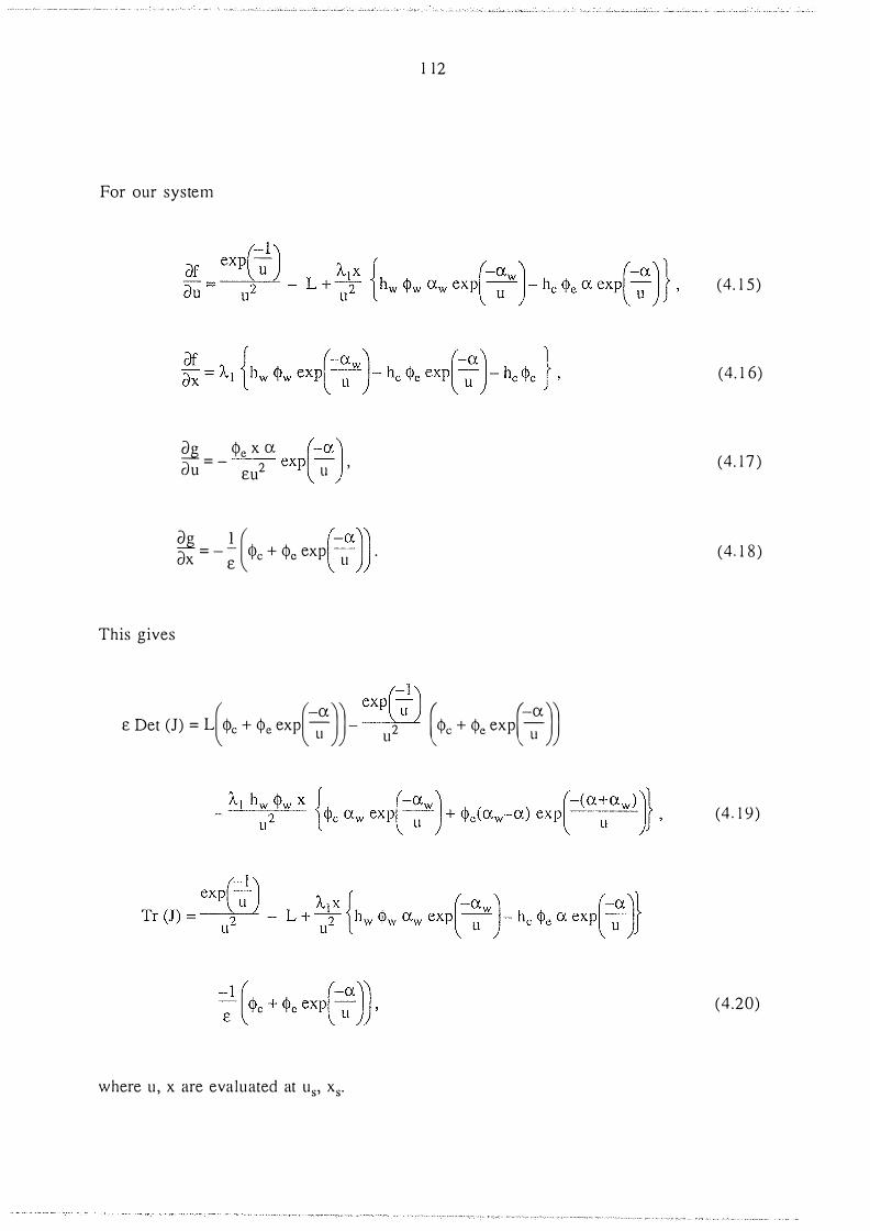
For our system

This gives

� = - <l>e x a exp(-aJ ' OU £U2 Ll

� l ( (-(J.,JJ ox = - £ <l>c + <l>e exp u .

1 12

PYn(:J..) ( (-(J.,JJ � ( (-(J.,JJ £ Det (J) = L <!>c + <l>e exp � - u2 <l>c + <l>e exp �

where u, x are evaluated at U5, X5.

(4. 1 5 )

(4. 1 6)

(4. 1 7 )

(4. 1 8 )

( 4 . 1 9 )

(4.20)

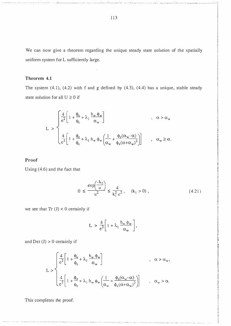
1 1 3

We can now give a theorem regarding the unique steady state solution of the spatially

uniform system for L sufficiently large. Theorem 4. 1

The system (4. 1 ) , (4.2) with f and g defined by (4.3) , (4.4) has a unique, stable steady

state solution for all U ;:::: 0 if

L >

Proof

Using (4 .6) and the fact that

( � ) 4 () ::; 2 ::; 22 (k l > 0) ' u k e ' I

we see that Tr (J) < 0 certainly i f

and Det (J) > 0 certainly if

L >

This completes the proof.

(4 .2 1 )

1 1 4

This result has a logical physical interpretation in that it predicts that if the surface area to

volume ratio of a body is suffi ciently large then criticality will not occur and so

spontaneous combustion is very unlikely. That is, if we take any moist self-heating body

and store it in , for example, the shape of a sufficiently thin brick , then the body will not

spontaneously ignite .

We will now derive some existence and uniqueness results for the sol ution of the time

dependent problem (3 .47) - (3 .50) . Firstly we make a comment on the use of Arrhenius

kinetics. The Arrhenius law, given for example for a single exothermic reaction by ( 1 .2)

i .e .

(-E) q (T) = QpZ exp RT ,

holds only for T ;.:::: 0. Since the function exr(��) has a singularity at T = 0 there is

obviously a problem in extending this theory to the range T < 0 (and non-dimensionally to

u < 0) . We will thus assume that, in effect, there is a Heaviside operator in front of each

temperature dependent Arrhenius term which 'switches the reaction off for T < 0. This

seems realistic physically since it is unlikely that any reaction will still be occurring at

'negative' absolute temperatures. We will not need to look at the range T < 0 in general in

this thesi s, but we do need to consider this range briefly here to derive a priori bounds for

the solution of the spatially unifom1 time dependent problem.

To consider the existence and uniqueness of sol utions to the time dependent spatially

uniform system (3 .47 ) - (3 . 50), we will first show that the solutions are bounded for all

time.

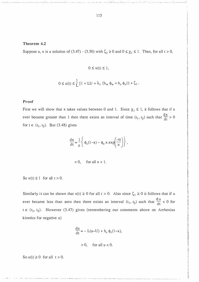
1 1 5

Theorem 4.2

Suppose u, x is a solu tion of (3 .47) - (3 .50) with �1 � 0 and 0 � x1 � 1 . Then, for all t > 0,

0 � x(t) � 1 ,

1 0 � u (t) � L [ 1 + LU + A] {hw <Pw + he <Pe J J + � 1 .

Proof

First we will show that x takes val ues between 0 and 1 . S ince X 1 � 1 , it follows that i f x ever became greater than 1 then there exis ts an interval of time (t1 , t2) such that �� > 0

for t E (t 1 , t2) . But (3 .48) gives

So x(t) � 1 for all t > 0 .

dx 1 { (-a) } dt = ; <Pe( l -x) - <Pe x exp u ,

< 0, for all x > 1 .

Similarly i t can be shown that x(t) � 0 for all t > 0. Also since � 1 � 0 it follows that if u

ever became less than zero then there exists an interval (t 1 , t2) such that �� < 0 for

t E ( t1 , t2) . However (3 .47) gives (remembering our comments above on Arrhenius

kinetics for negative u)

So u(t) � 0 for all t > 0.

du dt = - L(u-U) + he <Pe( l -x) ,

> 0, for all u < 0.

1 1 6

Finally, since 0 :::; x(t) :::; 1 , we have from (3 .47)

=> d . 1 d t ( exp(Lt)u) :::; exp(Lt) [ 1 + LU + 1\.1 { hw <Pw + he <Pc } J ,

1 exp (Lt) u :::; L exp(Lt) l 1 + LU + 'A1 { hw <Pw + he <Pc J J + Cs,

where C5 i s a constant of in tegration.

Now at t = 0, u = s 1 , so we can choose

which gives

Thi s completes the proof.

These a-priori bounds for the solutions of (3 .47) - (3 .50) can now be used to show that (3 .47) - (3 .50) has a unique solution if 0 :::; x 1 :::; 1 , s 1 � 0. This follows from classical

resul ts on ordinary differential equations given that f and g satisfy Lipschitz conditions on

some bounded set in IR 2.

1 1 7

4.3 The nature and stabi l i ty of steady state solutions

The local stabi lity of the steady states of the spatially uniform model can be determined by

looking at the stability of the first variation of (3 .47) , (3 .48) . Consider a system of the

form (4. 1 ) , (4.2) i .e.

du dt = f(u, x, §., � ) ,

dx dt = g(u, x , §., � ) .

Consider further a particular steady state solution us, xs such that

(4.22)

(4.23)

Now perturb us, xs by small amounts tlu, tlx i.e.

u = u5 + tlu, (4.24)

x = Xs + tlx, (4 .25)

then Taylor series expansions for f and g about us, x5 gives

df + dx (U5 , xs, §. , �) tlx + o((tlu) , (tlx)) ,

1 1 8

i!__g + ox (us, Xs, Q, �) L1x + o((L1u), (L1x)) .

Neglectin g terms of o((L1u) , (L1x)) , using (4.22), (4.23) and substituting into (4. 1 ) , (4.2)

gives the equations for L1u and L1x to leading order as

(4 . 26)

(4 .27)

which has a solution of the form

(4 .28)

(4.29)

where F1 , F2 , F3 , F4 are real constants and 0 1 and 02 are real or imaginary numbers . In

fact the values 01 and 02 are j ust the eigenvalues of the Jacobian matri x of the system

evaluated at the steady s tate, where the Jacobian i s as given i n (4. 1 2 ) . These

eigenvalues are given by the roots of the characteristic polynomial

02 - Tr(J)0 + Det(J) = 0. (4 . 30)

So we can see that the nature and stability of the steady state point us , Xs we are

considering, depends critically on the form of 0 1 and 02, given that 01 and 02 must either

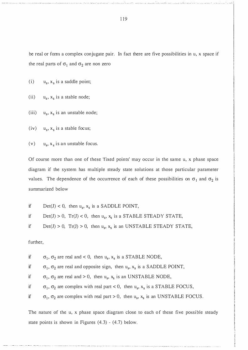
1 1 9

be real or fonn a complex conjugate pair. In fact there are five possibilities in u , x space if

the real parts of 01 and 02 are non zero

( i ) us , x s is a saddle point;

( i i ) us , xs i s a stable node;

(iii) us , xs i s an unstable node;

( iv) u5 , x5 is a stable focus;

( v ) us, x 5 i s a n unstable focus.

Of course more than one of these 'fixed poin ts' may occur in the same u , x phase space

diagram if the system has multiple steady state solutions at those particular parameter

values. The dependence of the occurrence of each of these possibilities on 0 1 and 02 is

summarized below

if Det(J) < 0, then u5, xs is a SADDLE POINT,

if Det(J) > 0, Tr(J) < 0, then us , xs is a STABLE STEADY STATE,

if Det(J) > 0, Tr(J) > 0, then us, xs is an UNSTABLE STEADY STATE,

further,

if 01 , 02 are real and < 0, then us , xs is a STABLE NODE,

if 01 , 02 are real and opposite sign, then us, xs is a SADDLE POINT,

if 01 , 02 are real and > 0, then us, xs is an UNSTABLE NODE,

if 01 , 02 are complex with real part < 0, then u5, x5 is a STABLE FOCUS ,

if 01 , 02 are complex with real part > 0 , then us, xs is an UNSTABLE FOCUS .

The nature of the u , x phase space diagram close to each o f these five possi ble steady

state points is shown in Figures ( 4. 3) - ( 4. 7) below.

X

X

1 20

u

Figure 4.3 Saddle point steady state

u

Figure 4.4 S table node steady state

X

X

12 1

u

Figure 4.5 Unstable node steady state

u

Figure 4.6 S table focus steady state

X

122

u

Figure 4.7 Unstable focus steady state

Other possibilities include: Det(J) = 0 , this is known as a saddle-node type bifurcation (or

i n our context a ' l imit point') and usually indicates a change in the stability of the steady

state solution ; Det(J) > 0, Tr(J) = 0, this corresponds to cr 1 , cr2 being complex conjugates

with zero real p arts and indicates the possibility of periodic solutions , i . e . a Hopf

bifurcation point; Det(J) = 0, Tr(J) = 0, this corresponds to cr 1 and cr2 being identically

zero complex numbers, and is known as a double zero eigenvalue degeneracy .

We will discuss periodic solutions and their stability near a Hopf bifurcation point in the

next section .

1 23

4.4 Hopf bifurcation points and periodic solutions

As we have stated in the last section, the conditions for a steady state solution u 5 , x5 to

also be a Hopf bifurcation point are

Tr(J) = 0, (4. 3 1 )

Det(J ) > 0 . (4 . 32)

Hopf bifurcations are important to locate because (i) they usually represent a point in

parameter space where a branch of periodic solu tions ( limit cycles) emanates from the

steady state branch and (i i) they earmark a change in the stab i l i ty of the s teady state

solutions. The exception to (i) occurs when the degeneracy condition

d (Tr(J) ) _ 0 dU - ' (4 . 33 )

i s satisfied. This corresponds to two Hopf bifurcation points coinciding a t the same point

on the steady state branch, so there are no emanating periodic branches linking them. The

set of conditions ( 4 .3 1 ) , ( 4 .32) , ( 4 .33) is known as the H21 degeneracy in the notation of

Gray and Roberts [ 49] , and we will investigate in detail its occurrence in parameter space.

We can calculate the stability of the limit cycles c lose to the Hopf b ifurcation point by

looking at the sign of a parameter we shal l refer to as IJ.s· The parameter is a function of

the first three partial derivatives of f and g evaluated at the Hopf bifurcation poi nt. To

calculate IJ.s we wil l follow the formula of Segel [52] , which we wi l l now outline.

1 24

At a Hopf bifurcation point the Jacobian matrix J given by (4. 1 2) will have purely imaginary conjugate eigenvalues ±ico0. To use the formula of Segel this coefficient matrix must have

the canonical form

0 } (4. 34)

If this is not the case for our original system at the Hopf bifurcation poin t then new

variab les

u = Pu u + P1 2 x,

X = P21 u + P22 X,

must be introduced so that the modified system

du -f - - � R) dt = ( u , x , �' � ,

dx _ _ _ � R) dt = g ( u , x , �, � ,

does have a Jacobian matrix of the desired form.

It is easily verified that

Pu = 1 ,

P12 = 0, lu

P21 = -, coo

Jl 2 P22 = -,

coo

(4. 35 )

(4 . 36)

(4 . 37)

(4. 38 )

(4 .39)

1 25

are correct choices for the transformation, where the components of J are evaluated at the

Hopf bifurcation point . Now we calculate the fol lowing p artial derivatives at the Hopf

bifurcation point.

a21 B - -

20 - a-2 , u

a 21 B - --

1 1 - a-a- ' U X

a21 B -o2 - a-2 , X

a31 B - -

3o - a-3 , ll

a31 B -1 2 - a-a-? , u x -

The scalar quanb� 1-ls i s then given by

a2g C2o = arr2 ,

(j2(r c - �

1 1 - (Jlf(JX: '

(j2(r c - ::::._Q_ 02 - ax:2 ,

(j3(r c - ::::._Q_

o3 - a-3 , X

a3-c = g 2 1 a-2a- . U X

(4.40)

( 4 .4 1 )

The above constitutes Segel 's formula. However i t i s more convenient to write the partial

derivatives in (4.40) in terms of the first three partial derivatives of f and g with respect to

u and x. We can do this by fmming the matrices P and Q where

1 26

1 ()

P = ( P 1 1 P 1 2 J = :!_u :!J1 ( 4.42) P2 1 P22 CDo CDo

Q = p-1 = ( q l l q 1 2 1 ()

J = -J l l CDo (4 .43)

q21 q22 J1 2 ] 12

Then

(4.44)

( 4 .45)

(4.46)

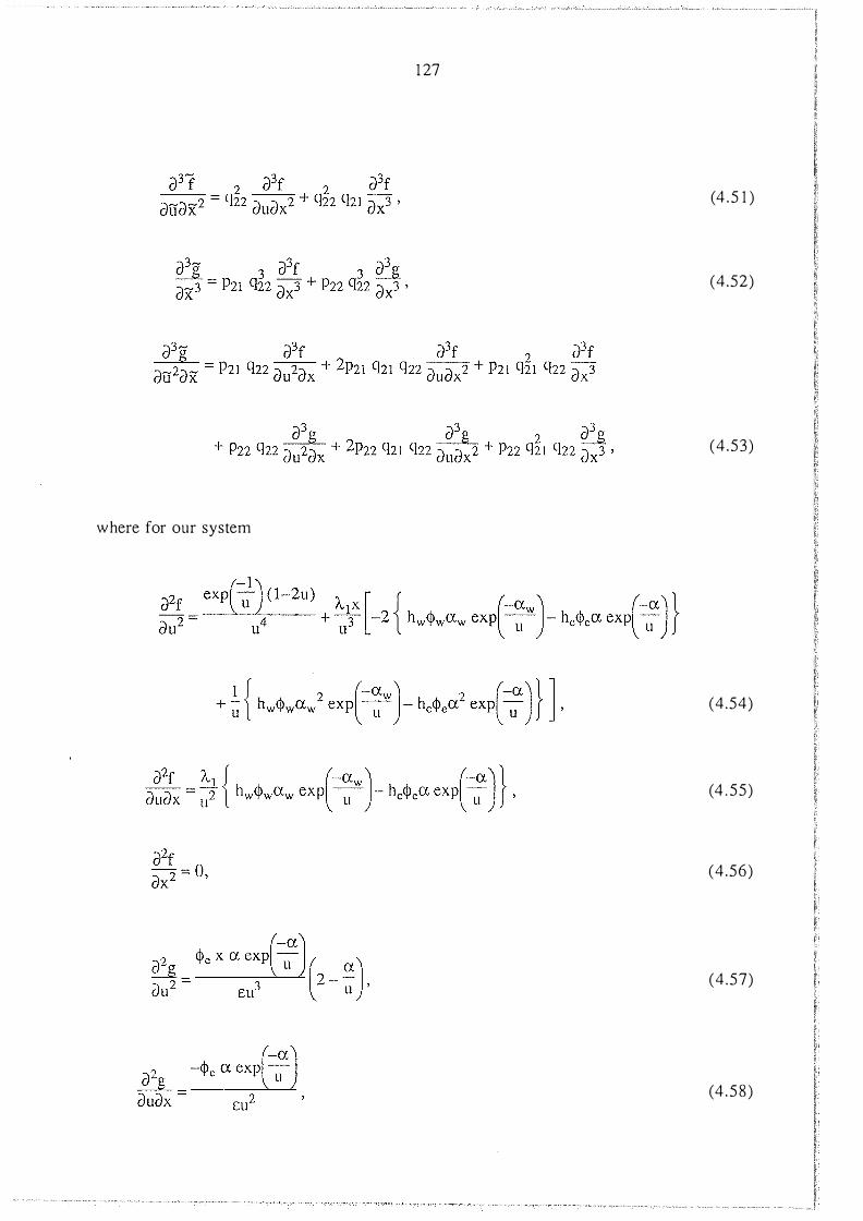
1 27

( 4 . 5 1 )

(4 .52)

(4 .53)

where for our system

(4.54)

(4 . 55)

(4 .56)

(4 .57)

(4 . 58 )

1 28

(-1 ) 2 ()3f exp u { ( 1-2u) ( l-4u) - 2u } 3A.l x [ { (-awJ 3 = 6 - 4 -2 hw<Pwaw exp -

dtr u u u

(4 .59)

(4 . 60)

( 4 . 6 1 )

( 4 . 62 )

(4 .63)

(4 .64)

(4 .65)

( 4 . 66)

1 29

These derivatives are to be calculated at u5, x5•

If lls i s negative then the limit cycles emerging from the Hopf bifurcation poin t will be

locally stable, if lls is positive then the emerging l imit cycles will be unstable.

The condition

lls = 0, (4 .67)

at a Hopf bifurcation poin t therefore corresponds to a change i n stability of the emerging

l imit cycles, and so represents another important phenomenon in parameter space. The

set of conditions (4. 3 1 ) , (4.32), (4.67) is known as the H3 1 degeneracy, in the notation of

Gray and Roberts [49] .

G . h . f h . . d d (Tr(J ))

h H f. b . . . . h h 1ven t e srgns o t e quanmres 1-ls an dU at t e op rturcanon pomt, t en , t e

four possibilities for the stability and direction of the loci of emerging limit cycles in the

neighbourhood of the Hopf bifurcation point are given schematically below in Figures 4 .8 -

4 . 1 1 . I n these diagrams (as in all later U, u bifurcation diagrams) a broken line represents

an unstable s teady state, an unbroken line represents a stable steady state, an open circle

represents an unstable periodic solution and a b lack circle represents a stable periodic

solution .

•

increasing U

Figure 4.8 Nature of the emerging l imit cycles in the neighbourhood of a Hopf d(Tr(J))

0 bifurcation point for lls < 0, dU > ·

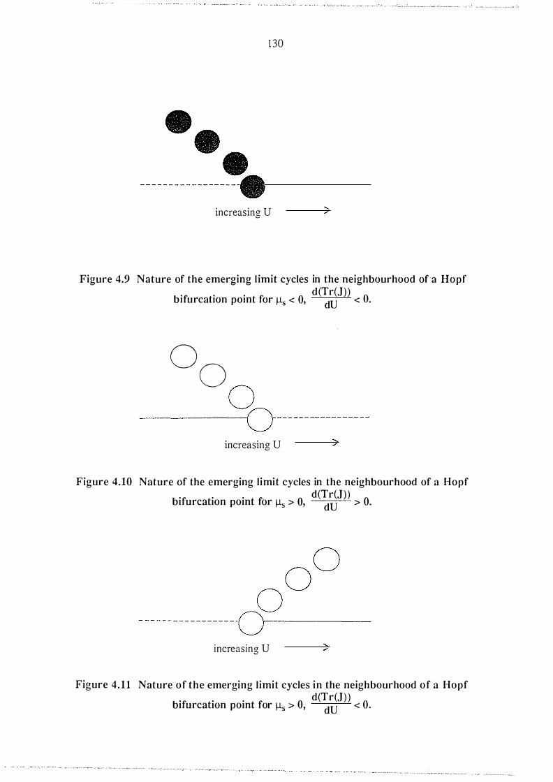
130

increasing U

Figure 4.9 Nature of the emerging l imit cycles in the neighbourhood of a Hopf d(Tr(J))

0 bifurcation point for lls < 0, dU < ·

00 0 ----------��-----------------

increasing U

Figure 4.10 Nature of the emerging l imit cycles in the neighbourhood of a Hopf d(Tr(J) )

0 bifurcation point for lls > 0, dU > ·

00 0 - - - - - - - - - - - - - - - - -�--------------------

increasing U

Figure 4 .11 Nature of the emerging l imit cycles in the neighbourhood of a Hopf d(Tr(J) )

0 bifurcation point for lls > 0, dU < ·

13 1

There are two possibi l i ties for the u l timate destin ation of a locus of limit cycles from a

Hopf b ifurcati on po in t. I t can ei ther rejoin a steady s tate branch at another Hopf

bifurcation point , or the locus can abruptly end (or 'evaporate') before reaching another

Hopf bifurcation point. This 'evaporation' corresponds to the period of the l imit cycle

becoming infinite as the amplitude of the limit cycle grows to such an extent that the limit

cycle meets the separatrices of a saddle point in phase space. The 'evaporation ' of a limit

cycle in phase space is i l lus trated in Figures 4. 12 - 4. 14.

X

� -----

u

Figure 4.12 Limit cycle in proximity of saddle point.

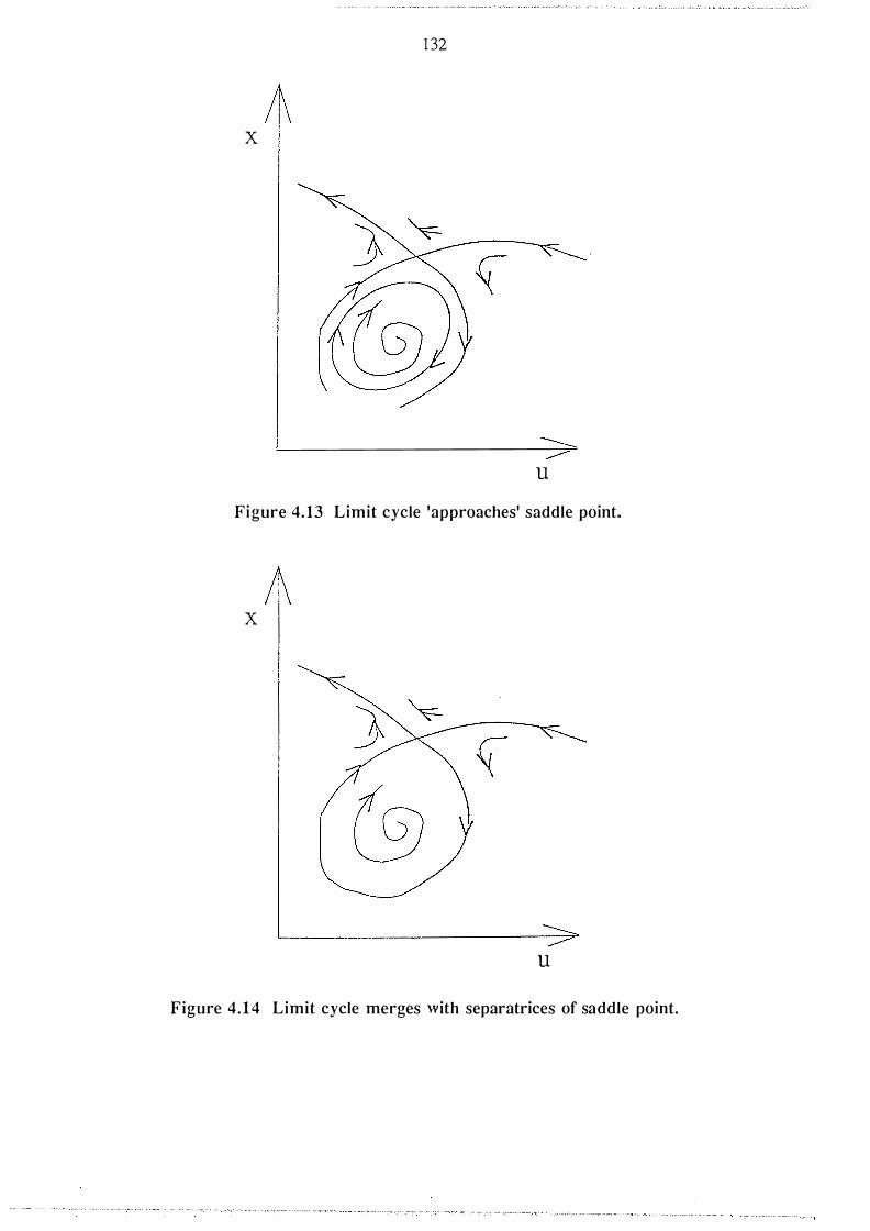
1 32

X

u

Figure 4. 13 Limit cycle 'approaches' saddle point.

X

u

Figure 4 .14 Limit cycle merges with separatrices of saddle point.

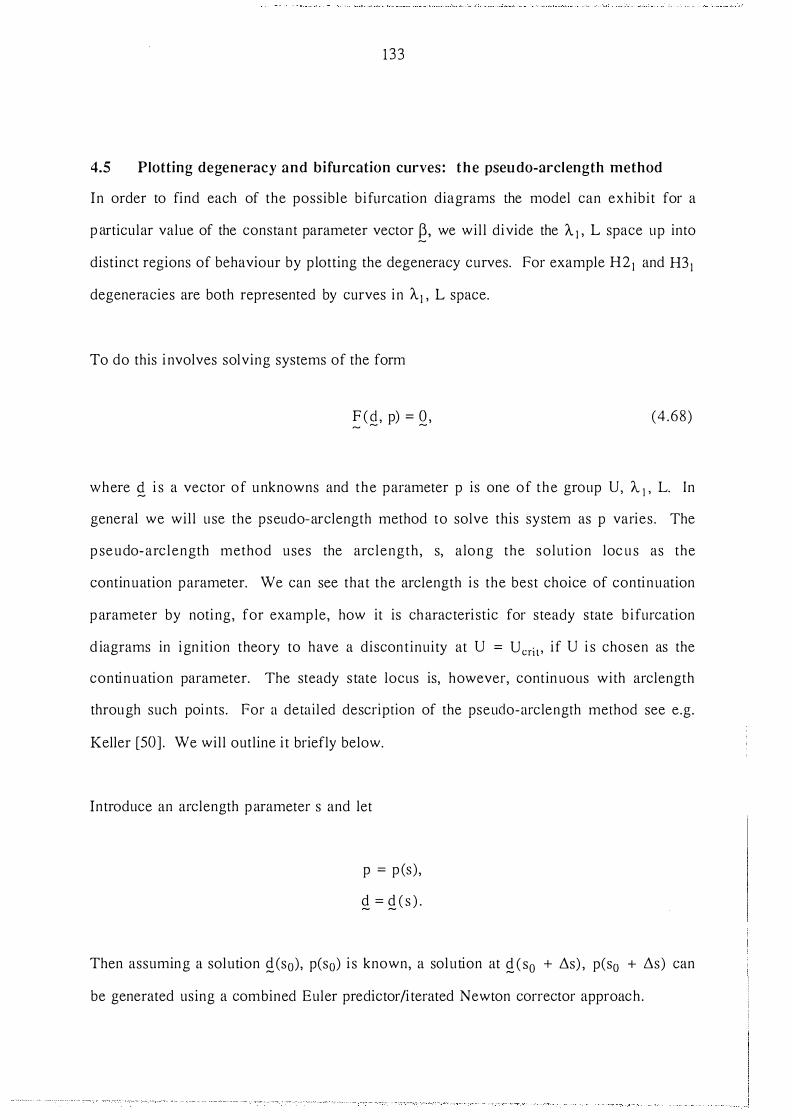
133

4.5 Plotting degeneracy and bifurcation curves : the pseudo-arclength method

In order to find each of the possible b ifurcation diagrams the model can exhibi t for a

p articular value of the constant parameter vector � ' we wil l divide the A 1 , L space up into

distinct regions of behaviour by plotting the degeneracy curves. For example H21 and H3 1

degeneracies are both represented by curves in A1 , L space.

To do this i nvolves solving systems of the form

F ( d , p) = 0 , �

� � (4 .68)

where Q i s a vector of unknowns and the parameter p is one of the group U, A 1 , L. In

general we wil l use the pseudo-arclength method to solve this system as p varies . The

p seudo-arclength method uses the arclength , s, along the solut ion loc u s as the

continuation parameter. We can see that the arclength is the best choice of continuation

parameter by noting, for example, how it is characteri stic for steady state b ifurcation

d iagrams in ign ition theory to have a discontinuity at u = ucri l' i f u i s chosen as the

continuation parameter. The steady s tate locus is, however, contin uous with arclength

through such poi nts. For a detai led description of the pseuclo-arclengrh method see e.g.

Keller [50] . We will outline i t briefly below.

Introduce an arclength parameter s and let

p = p (s) ,

£ = £ ( s ) .

Then assuming a solution £(s0), p(s0) i s known, a solu tion at £ ( s0 + ils) , p(s0 + ils) can

be generated using a combined Euler predictor/i terated Newton corrector approach.

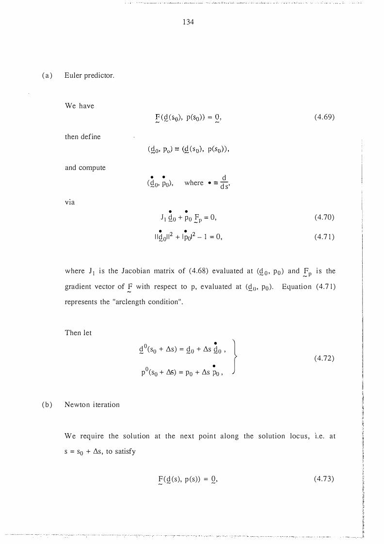
( a ) Euler predictor.

We have

then define

and compute

v1a

• •

1 34

( £o, Po), where

• •

d · = -- d s'

J 1 £o + Po �p = O, • 2 • 2 11£011 + l p01 - 1 = 0,

(4 . 69)

(4.70)

(4.7 1 )

where J 1 i s the Jacobian matrix of (4.68) evaluated at (£ 0, p0 ) and EP i s the

gradient vector of � with respect to p, evaluated at (£0, p0) . Equation (4.7 1 )

represents the 1 1

arclength condition 1 1

•

Then let

( b ) Newton i teration

d0(s + ils) = d + ils d , } _ o _o _o

• p

0(s0 + t:l5) = p0 + t:ls Po ,

(4.72)

We require the solu tion at the next poin t along the solut ion locus , I .e . at

s = s0 + t:ls, to satisfy

F (d (s) , p (s)) = 0 , -

- -(4.7 3)

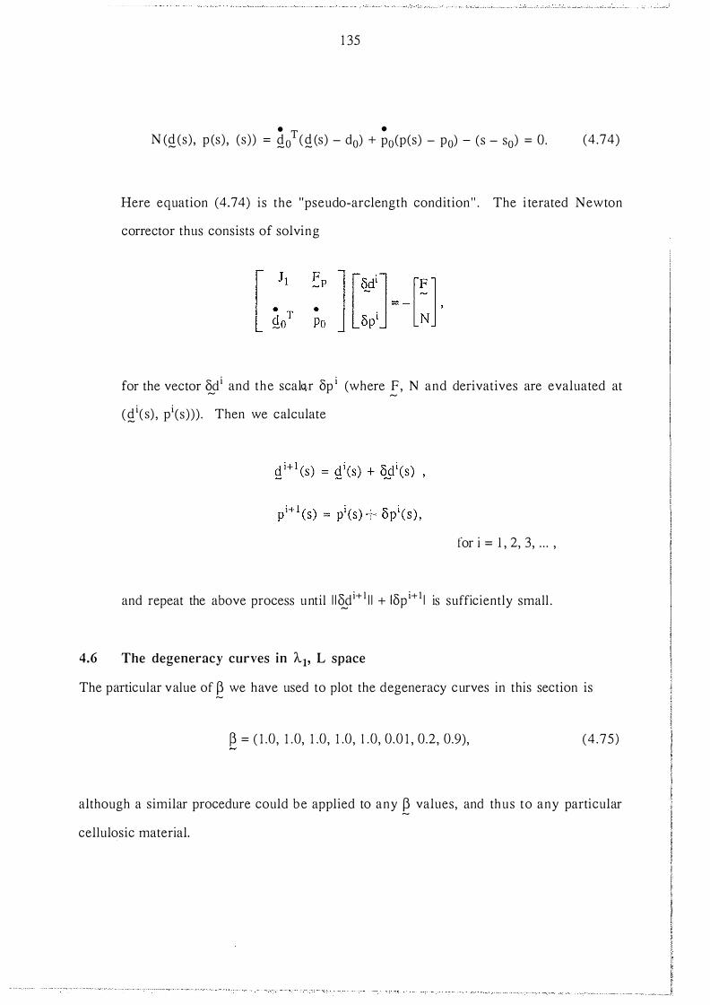
1 35

• T • N (£(s), p (s) , (s)) = £0 (£ (s) - d0) + p0(p(s) - p0) - (s - s0) = 0. (4 .74)

Here equation (4.74) is the "pseudo-arclength condition" . The i terated Newton

corrector thus consists of solving

for the vector 8d i and the scalqr 8p i (where F, N and derivatives are evaluated at � �

(£i( s) , pi(s))) . Then we calculate

for i = 1 , 2, 3, . . . ,

and repeat the above process until l l�i+ l l l + 18p i+ l l is suffic iently small .

4.6 The degeneracy curves in A-1, L space

The particular value of � we have used to plot the degeneracy curves in this section is

� = ( 1 .0, 1 .0, 1 .0, 1 .0, 1 .0, 0.0 1 , 0.2, 0.9), (4 .75)

although a similar procedure could be applied to any � values, and thus to any particular

cellulosic material.

136

4.6.1 The hysteresis and double l imit point curves

The hysteresis curve in A. 1 , L space corresponds to a curve along which l imit points are

born on the U , u bifurcation diagram. The equations which must be satisfied by the

hysteresis curves are the s teady state condi tion (4.7) as well as

(4 .76)

and

(4.77 )

where

(4 .78 )

(4.79)

and

(4 . 80)

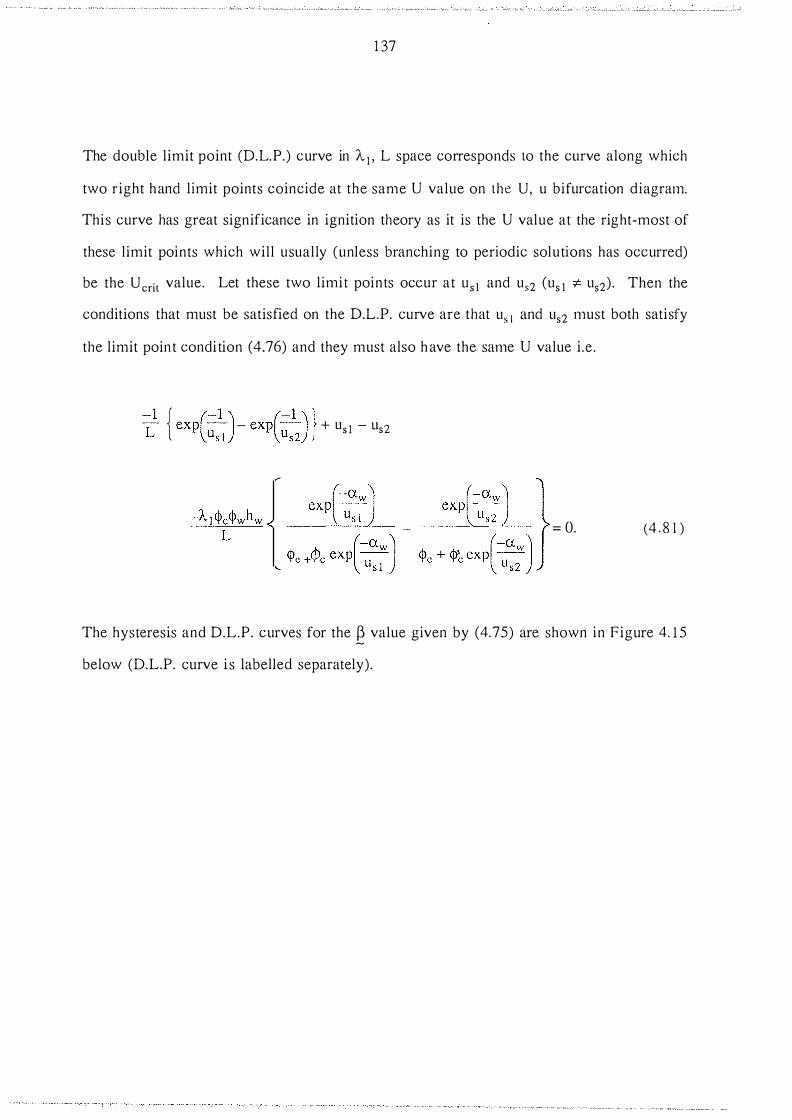
1 37

The double limit point (D.L.P.) curve in A. 1 , L space corresponds to the curve along which

two right hand limit points coincide at the same U value on the U, u bifurcation diagram.

This curve has great significance in ignition theory as it is the U value at the right-most of

these limit points which wil l usually (unless branching to periodic solu tions has occurred)

be the Ucrit value. Let these two limi t points occur at u5 1 and u52 (u5 1 :;t:. u52) . Then the

conditions that must be satisfied on the D.L.P. curve are that us 1 and u52 must both satisfy

the limit poin t condi tion (4.76) and they must also have the same U value i .e.

i1 { exp(:slJ- exp(:s�) } + Us l - Us2

= 0. (4 . 8 1 )

The hysteresis and D.L.P. curves for the � value given by (4.75) are shown in Figure 4. 1 5

below (D.L.P. curve i s labelled separately).

4 . 0 0 1 L

3 . 0 0 j 2 . 0 0

1 . 0 0

0 . 0 0 0 . 0 0

I I I I I I I I

0 . 5 0

1 38

I 1 .00

'\ D .L . P .

Figure 4 . 1 5 Hysteresis and D.L.P. curves

I I I I I I 2 . 0 0

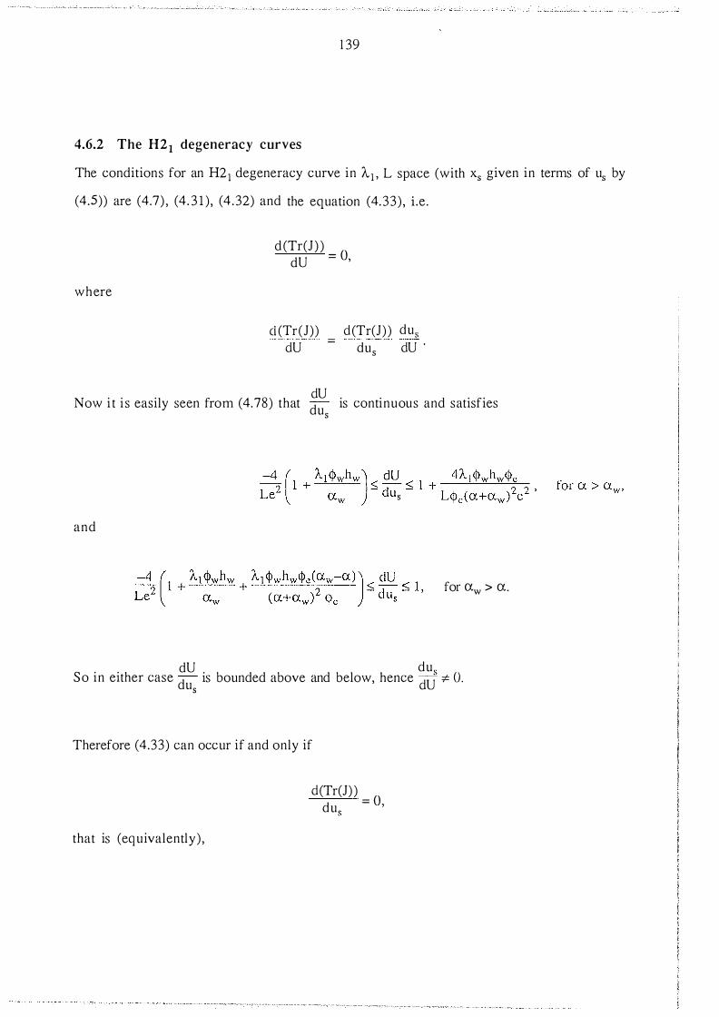
1 39

4.6.2 The H21 degeneracy curves

The conditions for an H21 degeneracy curve in A-1 , L space (with x5 given in terms of u5 by

(4.5)) are (4.7) , (4. 3 1 ) , (4 .32) and the equation (4.33) , i .e .

where

d (Tr(J ) ) _ 0 dU - '

ci (Tr(J)) ciU

ci (Tr(J) ) clu5 = clu5 ciU ·

ciU Now i t i s easily seen from (4.78) that is continuous and satisfies du5

and

for aw > a.

dU clu5 So in either case dus is bounded above and below, hence ciU :t= 0.

Therefore (4.33) can occur if and only if

ci(Tr(J) ) cl =

0

that is (equ ivalently) ,

u ' s

140

(4.82) E

The H21 degeneracy curves for the given � value are shown below in Figure 4. 1 6. The

dashed line corresponds to a portion of a curve along which Det(J) < 0 and is included only

for completeness.

L

4 . 0 0 j

� l l l J I

3 . 0 0 I 1 I l J J I

J 2 . 0 0 I I

� 1 . 00 �

� l J I ]- - -2- - - - - -

I C . J O ,:��7. ,,-.. �.-.. �.-., �.-. . •. �. 7, •. �. �. -,�, �.��-.�7>.-... :

O . C C C . SC LOG 1 . 5G

Figure 4 . 16 H21 degeneracy curves

1 4 1

4.6.3 T h e H3 1 d egeneracy curves

The equations defin ing H3 1 degeneracy curves in A.1, L space are (4.7), (4. 3 1 ), (4.32) and

(4.67), wi th x5 given in tenns of u5 by (4.5). Figure 4.17 below shows the H31 degeneracy

curves for the chosen value of �·

3 . 0 0

2 . 0 0

1 . 0 0

� J J I J

l 0 . 0 0 �, ,,�, -., ,,��, ,,-., -rl �,-rl ��, �, ��, �,�,�, ��, �,��,-,�, ��-., �,-., �,-., ,,-., -,11-ril i 0 . 0 0 0 . 50 1 .00 1 .50 2 . 0 (

AI Figure 4.17 The H31 degeneracy curves

142

4.6.4 T h e double zero eigenvalue curves

A double zero eigenvalue (D.Z.E.) point in A.1 , L space usually corresponds to the abrup t

appearance (or disappearance) of a Hopf bifurcation point on the U, u bifurcation diagram.

The equations the D . Z.E. curve must satisfy are (4.7), (4.3 1) and

Det(J) = 0, (4 . 8 3 )

where Det(J) i s given b y (4. 1 9) , (wi th x5 given in terms of u5 by (4.5)) . The D .Z.E.

curves for our value of � are given below in Figure 4. 1 8.

4 . 0 0 I J J

L J J I J I

3 . 0 0 I I I I

� � l

2 . 0 0 I I l I l l l J �

1 . 0 0 l I � l J

I I J i

0 n e l . v . I '

C· . C· C: ; i I l I i i l I I i I I 1 1 i ' I I I I I 1 1 i I I I I 1 I I I I I I

C . 5 0 1 .00 1 . 50 2 . 0 C AI

Figure 4. 18 The D.Z.E. curves

Note

4.7

1 43

d2u d2U S ince by (4.79), --2 ---t 0 as us ---t 0 and us ---t oo, and -

d 2 is conti nuous in us , we 2 dus us

have dd � :F ro, V us > 0. Therefore, using the condition of Gray and Robens [ 49J us

p 367, the system has no isolas or transcritical bifurcations.

The distinct bifurcation diagrams

Our aim in this section is to find all the distinct U , u bifurcation diagrams the model can

exhibi t for the value of � given by (4.75) , and thus all the possible steady s tate and

periodic behaviour of the model as the group of parameters � varies. We can do this by

simply superimposing all the curves p lotted in the previous section on the same A 1 , L

diagram. Each c losed region on this new diagram will correspond to a set of A 1 , L values

which give a distinct bifurcation diagram in U , u space.

The superimposed degeneracy curves are given below in Figure 4. 19. Figure 4 .20 shows

a blow up of the part of Figure 4. 1 9 with A 1 E [0, 0 .5 ] , L E l 0. 0 .6j . The distinct regions

are given labels 1, . . . , 25.

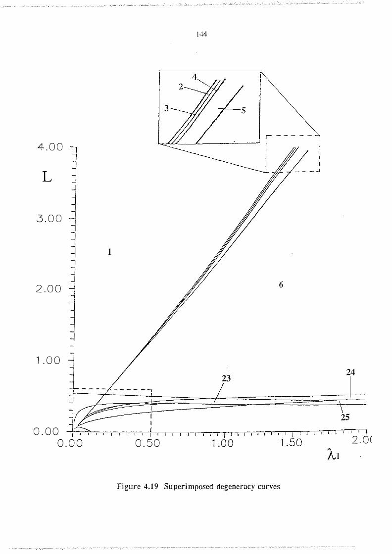
4 . 0 0

L

3 . 0 0

2 . 0 0

1 . 0 0

� l l j J

� l J I

� l -i i _ _ _ _

144

5

r - - - - -1.....::::-''...LL._.J-__ ___:__� ,

1

6

23 24

- - - - - -,

25

0 . 0 0 _l�l �� , �� , �,�, �, �,�� -. �, ��,-., ,, ,,-r, 11, I 0 . 0 0 0 . 5 0 1 .0 0 2 . 0 (

Fi gure 4.19 Superi mposed degeneracy curves

145

8,9,10,11 7

12 ----t-

13

t 18 19 21 22

Figure 4.20 B low-up of region near origin

Figures 4.2 1 - 4.45 below show schematicaHy the twenty-five distinct U, u bifurcation

diagrams possible for the given value of �-

• . .,'

._ ......... ./'

Figure 4.21 B i furcation diagram Figure 4.22 B ifurcation diagram

for region 1 for region 2

u

• • • • . , ,

00 ��",./

Figure 4.23 B i furcation diagram

for region 3


for region 5

1 46


for region 4


for region 6

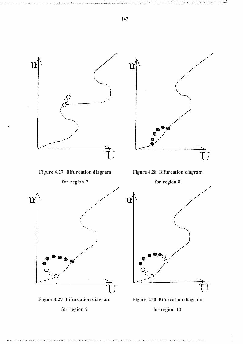
, r \ \ \

' ' - --..... , " \

l

/ \ \ " " '---... " \ I

Figure 4.27 B i furcation d iagram

for region 7

\ \ ' ''-- - .... ' \ I


for region 9

147

\ \ ', '---.... ' \

I

Figure 4.28 Bi furcation diagram

for region 8

, , , , , ,·-'

\ \ ',

'---.... \ \ I

Figure 4.30 Bi furcation d iagram

for region 10

/ I \ ' '

'-- .... .... ' \ I

• • 0 '\ ---------

. ,' I \ 41 ',, --- ' . ';

0 / 0 /�/

� Figure 4.31 Bifurcation diagram

for region 1 1

Figure 4.33 Bifurcation diagram

for region 13

148

I \ " ' "--.... .... ' \ l

Figure 4.32 Bifurca tion diagram

\ \ ',,

for region 12

-- --

... , ...

·-

- ----

- - --

- - - - - - - -

-.

oo / .�.?�

_________. /

I I I

I

tf Figure 4.34 Bifurcation diagram

for region 14

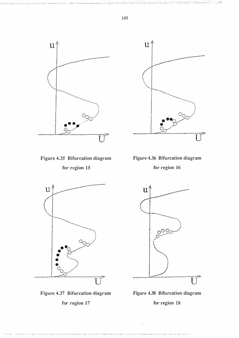
u

' '

'' ....... ',

... - - -� ... ',

, '', ,,' •, ,,

' ', - ... - ... , ' ' I I

oo / · · ·�J-

__Jg/ tf Figure 4.35 Bifurcation diagram

for region 15

tf Figure 4.37 Bifurcation diagram

for region 17

l49

ll '


for region 16

-,,,, __ _ '''- - , ·,,

\ I

_? __ )

, i \ \

\ ,_

-, '"'"-... ,

' \ I . ,


for region 18

' '-, -------.... _ _ _ _ _ _ _ _ -----.... ,,

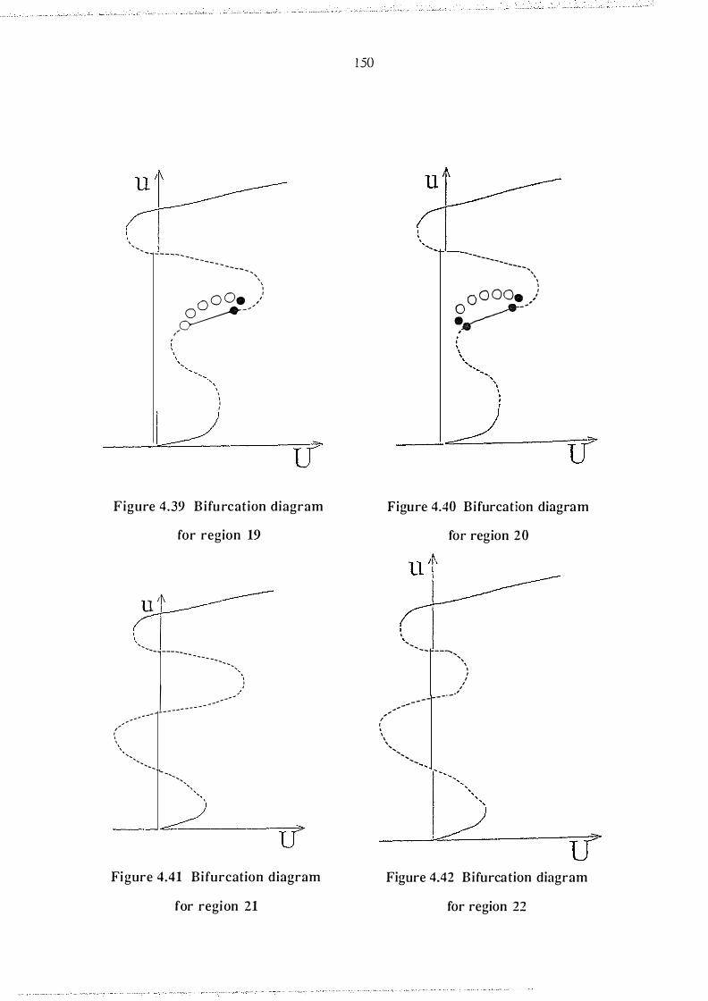
\ I

O o Oe / ,'�-'

' ' I I

�� Figure 4.39 Bifurcation diagram

for region 19

u /�

.._ I , ____ 1 ___ ___ _ --- -------- l -

-- --

--

---

-- -

-- - -

- - -- -

..... ... ..... ( ' ' ' '

............. ........... �

--

..................

� tf Figure 4.41 Bi furcation diagram

for region 21

150

---------------,, \ I

0 o OOe / ��--


,-

for region 2 0

' --------...

....... ,, ------- · -

-- ·'

I I

I I

I ," I \ \ ' '

........................ _ --])_

tr Figure 4.42 Bifurcation diagram

for region 21

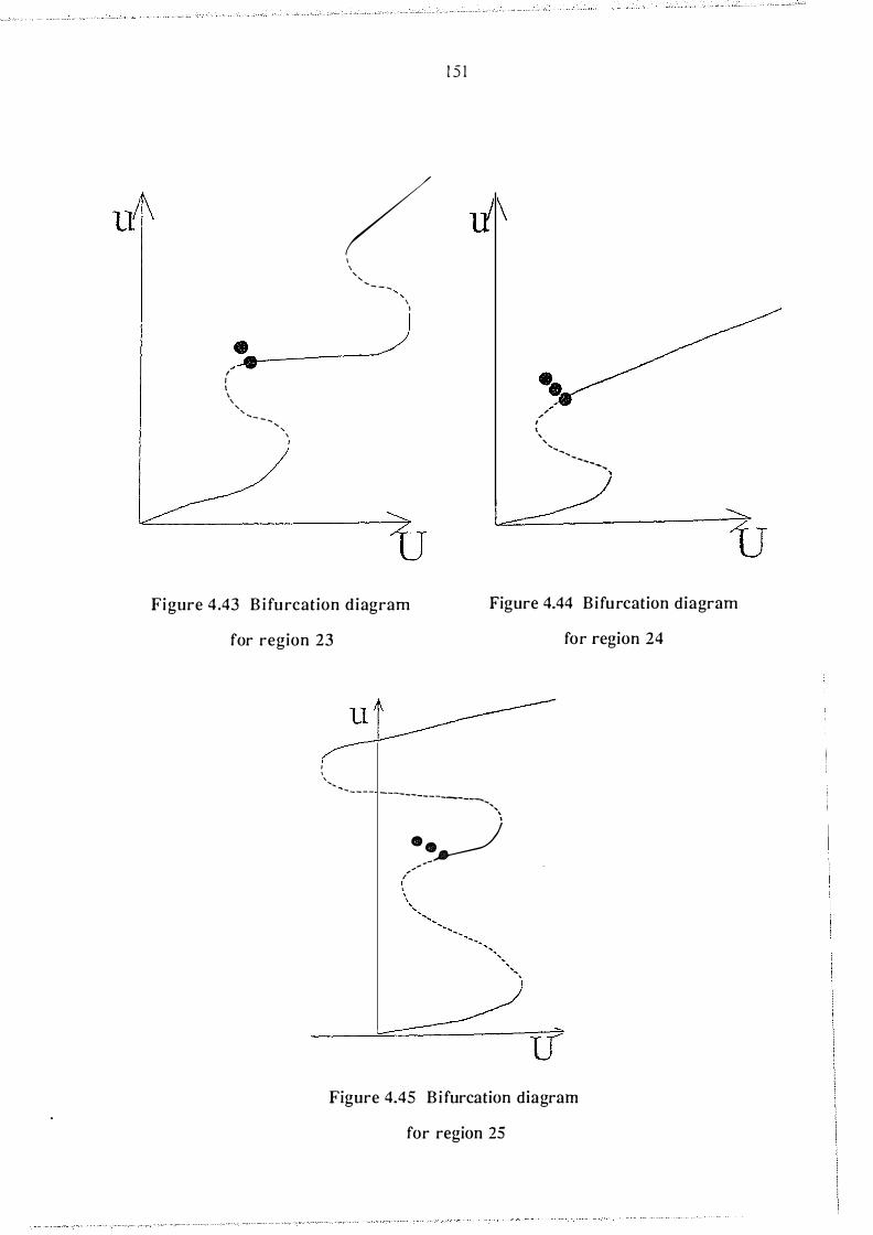
ll

! 5 1

/ I \

'

' � ---' \ 1

. ....___ __ ) #_. I I I \

'

', '--...... ,

\

I k=/ Figure 4.43 B i furcation d iagram

I \

., , '

' ................ ... __ _

��----7" 1J for region 23


for region 24

� I I '

\ ,_

, _ _ _ _ -------- - -----------, \

'

· ·� --i' .... --


for region 25

1 52

As we can see from the diagrams above the spatially uniform model including the effects of

moisture exhibits a very wide range of behaviour when compared to the model which

ignores the moisture content (i .e . A. 1 = 0). In fact the 'dry' model can show only two

distinct bifurcation diagrams (namely those corresponding to regions 1 and 1 2) .

An important point to note about this particular formulation of the variables (i .e . that of

B urnell et al [ 1 2] ) is that the s teady state and periodic loci can move into the negative U

section of the bifurcation diagram. Since the body will not be stored at or below absolute

zero the solutions in this section are irrelevant physically, although we are in terested in

following them to see where (and if) they re-enter the positive U section of the diagram.

This phenomenon does not lead to any computational difficulties in the spatially uniform

case (as we can see from the diagrams , u5 2:: 0 always) , but it will certainly lead to

difficulties if s teady s tate profiles are to be calculated for the spatially distributed model

(as there will always be a portion of the profile with u5 < 0). We will not consider this

phenomenon further in this thesis , but the solution will obviously involve usmg a

Heaviside operator in front of all Arrhenius terms, as discussed in section 4.2.

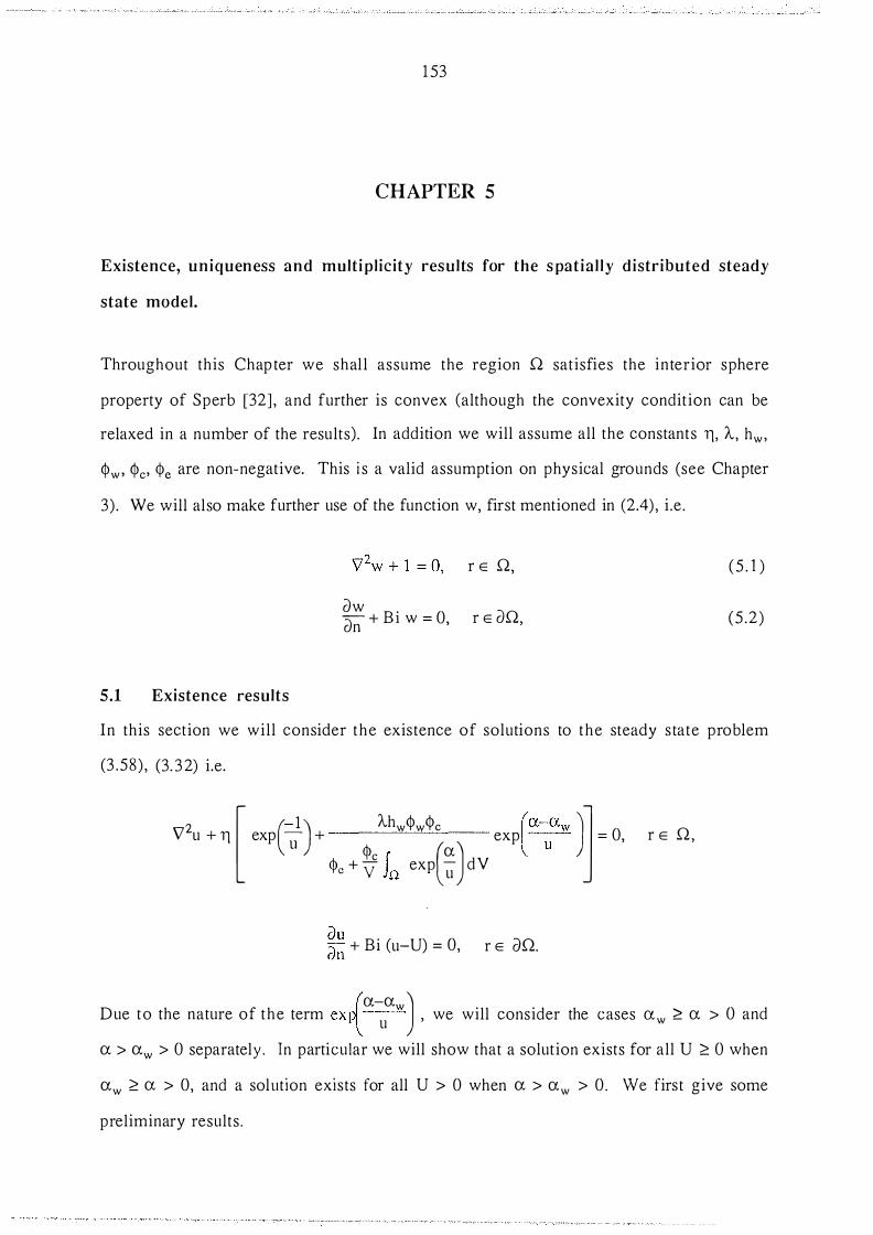
1 53

CHAPTER 5

Existence, un iqueness and mult i pl icity results for the spat ia l ly d istributed steady

state model.

Throughout this Chap ter we shal l assume the region Q satisfies the interior sphere

property of Sperb [32] , and further is convex (although the convexity condition can be

relaxed in a number of the results). In addition we will assume all the constants 11, A, hw, <J>w, <J>c, <Pc are non-negative. This i s a valid assumption on physical grounds (see Chapter

3). We will also make further use of the function w, first mentioned in (2.4) , i .e .

5.1 Existence results

aw B . 0 - + l W = an '

r E Q,

r E aQ,

(5 . 1 )

(5 .2)

In this section we wil l consider the existence of solutions to the steady s tate problem

(3 .58) , (3. 3 2) i.e.

2 [ (-1 ) Ahw<l>w<l>c (a-aw )'j V u + 11 exp u + <1> a exp -u- = 0,

<!> + ___s;_ r exp(-) dV e V Jn u

�u + Bi (u-U) = 0, r E an. Ull

r E Q,

Due to the nature of the term ex{ CJ.-uaw) , we will consider the cases CJ.w ;:, a > 0 and

a > aw > 0 separately . In particular we will show that a solution exists for all U :?: 0 when

aw :?: a > 0, and a solution exists for all U > 0 when a > aw > 0. We first give some

preliminary results.

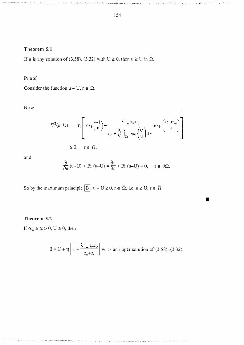
1 54

Theorem 5. 1

If u is any solution of (3 .58) , (3 . 32) with U � 0, then u � U in .Q.

Proof

Consider the function u - U, r E .Q.

Now

and

s 0, r E .Q,

:n (u-U) + Bi (u-U) = �� + Bi (u-U) = 0, r E an.

So by the maximum principle [!TI' u - u � 0, r E Q, i .e. u � u' r E n.

Theorem 5.2

If aw � a > 0, U � 0, then

[ Ahw<!>w<!>c] � = U + 11 1 + w is an upper sol ution of (3 .5 8) , (3 .32). <l>e+<l>c

•

1 55

Proof

The function � satisfies

and

[ Ahw<Pw<Pc ] [ (-1 J Ahw<Pw<Pc (a-awJ ] = -'11 1 + + '11 exp - + exp -- , <Pe + <Pc � <Pc J (aJ � <P + - exp - dV e V n �

::;; 0, r E Q,

_ [ 1 Ahw<Pw<Pc J (aw B . ) B . U - '11 + a + 1 w + 1 , <Pe + <Pc n

= Bi U, r E 8Q.

So, by Definition 2. 1 .6, � is an upper solution of (3 .58) , (3.22).

•

Theorem 5.3

If aw ;::: a > 0, u ;::: 0, then

is a lower solution of (3 .58) , (3 .32).

Proof

The function \jf satisfies

and

1 56

l (-1 ) Ahw<l>w<l>c (a-aw) j + TJ exp - + - exp --

,

W � (a) W · <l>e + - r exp - dV V Jn 'Jf

� 0, r E Q (by Theorem 5 . 1 ) ,

= Bi U, r E an.

So, by Definition 2. 1 .6 , 'I' is a lower solution of (3 .58) , (3 . 32) .

1 57

We can now give an existence result for the case aw � a > 0, U � 0.

Theorem 5.4

If aw � a > 0, U � 0 there exists a solution u to (3 .58) , (3 .32) with

r e Q.

Proof

For this proof we will use Theorem 2. 1 .7 . Now w(r) > 0, r E Q (by Theorem 2. 1 . 8 ) so

r e Q.

It i s easily shown that J (u)(h) , defined in Theorem 2. 1 .7 , for (3 .58) , (3 .32) satisfies

J(u)(h) = 11

� 0, if aw � a > 0, r E Q.

h

exp(� J 2 h dV , u

(5 .3)

1 58

Therefore, by Theorem 2. 1 .7 , there exists a solution u with

r E n.

Further to these results , we can show that any solution of (3 .58) , (3 .32) must lie between

these upper and lower solutions. We do this using Theorems 5 .5 and 5 .6 below.

Theorem 5.5

If aw 2 a > 0, U 2 0 and u is any solution of (3 .58) , (3 .32) , then

Proof

u ::;; u + 11 [ 1 + Ahw<l>w<l>c] W, r E n.

<l>e + <l>c

{ [ Ahw<J>w<l>c] } Consider the function u - u + 11 1 + w ' r E n.

<Pc + <Pc

Now

n2 ( { [ Ahw<Pw<l>c] }) l (-1 ) Ahw<Pw<Pc (a-aw J] v u - U + 11 1 + w = - 11 exp - + exp --<l>c + <Pc U <Pc (a) U

<Pc + y JQ exp u dV

2 0, r E .Q,

1 59

and

a ( { [ A-hw<Pw<Pc] }J ( { [ A-hw<Pw<Pc] }J an u - U + 11 1 + <Pe + <Pc

w + Bi u - U + 11 1 + <Pe + <Pc

w

au . [ A-hw<Pw<Pc] (aw . ) = an + B1(u - U) - 11 1 + <Pe + <Pc an + B1 w ,

= 0, r E aQ.

rAl { [ Ahw<Pw<Pc] } So by the maximum principle � , u - U + 11 1 + w � 0, <Pe + <Pc

i .e. r E Q.

Theorem 5.6

If aw ;;::: a > 0, U ;;::: 0 and u is any solution of (3 .58) , (3 .32), then

Proof

Consider the function

r E Q,

r E Q.

•

r E Q.

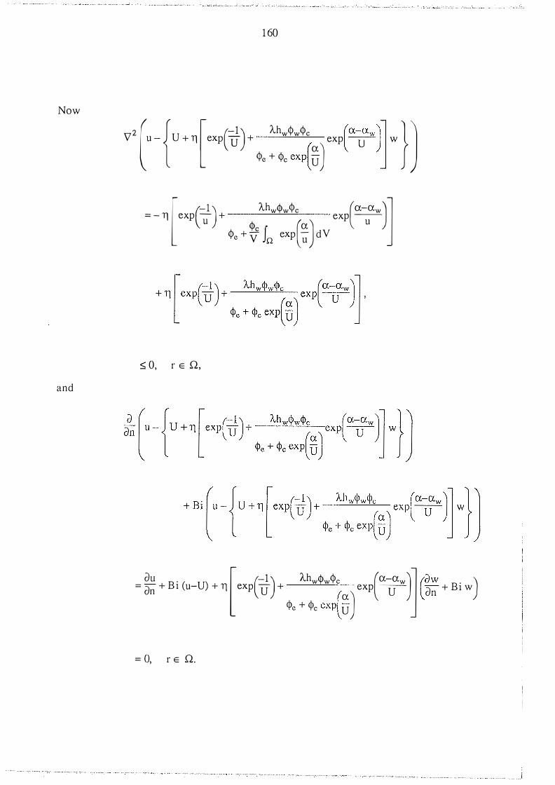
Now

and

1 60

V u - U + 11 exp 0 + a exp -U- w 2 [ { [ (-1 ) Ahw<l>w<l>c (a-aw)� }J

<l>c + <l>c exp( U) [ (- 1 ) A.hw<!>w<l>c (a-aw)l = - 11 exp u + <!> (a) exp -u <l>c + y Jn exp � dV

:::; 0, r E Q,

= dn + B i (u-U) + 11 exp U + a exp u- dn + Bi w du [ (-1 ) A.hw<!>w<l>c (a-aw)j (dw )

$, + $, exp( U) = 0, rE Q.

1 6 1

So, by the maximum principle � '

Le.

We now derive corresponding results for the case a > aw > 0.

Theorem 5.7

If a > aw > 0, U � 0 then

is a lower solut ion of (3 .58) , (3 . 32).

Proof


2 [ (-1) Ahw<Pw<Pc (a-aw)] \7 \jf + 11 exp -;- + <Pc a exp �

<Pe + - f exp(-) dV V Jn ,11

� 0, r E Q,

-

r E Q.

11

and

= B i U, r E an.

1 62

So by Definition 2. 1 .6 , \Jf is a lower solution of (3 .58) , (3 .32)

Theorem 5.8

If a > aw > 0, U > 0 then

is an upper solution of (3 .58) , (3.32).

Proof


:::;; 0, r E Q,

Ill

r E Q,

and

163

a� [ A.hw<l>w<l>c (a-awJil (a w ) an + Bi � = 11 1 + <l>e + <l>c exp u- � an + Bi w + Bi U,

= Bi U, r E an.

So, by Definition 2. 1 .6 , � is an upper solution of (3 .58) , (3 .32) .

•

Note : Clearly the above upper solution becomes infinite at U = 0, indeed we h ave been

unable to find an upper solution that holds for a > aw > 0, U = 0. It should be

noted again , however, that in physical situations an absolute zero ambient

s torage temperature is unlikely to arise.

Theorem 5.9

If aw > a > 0, U > 0 there exists a solution u to (3 .58) , (3 .32) with

r E Q.

Proof

We wil l again use Theorem 2. 1 .7.

It is easily shown that

U + 11 1 + exp u- W � U + 11 exp U + W, f E Q. [ Ahw<l>w<l>c (a-awJ� l (-1 ) Ahw<l>w<l>c J � + � (aJ <l>e + <l>c exp U

1 64

Also from (5 .3) we have

n A-h tt. tt. (a -a) (a-a ) J(u)(h) ;;::: , I w't'w't'c �2 exp U h . <Pc + <Pc

S o the positive constant 8 we must choose in this case to satisfy the conditions of

Theorem 2. 1 .7 is

Then, by Theorem 2. 1 .7 , there exi sts a solution u with

r E Q.

Theorem 5.10

If a > aw > 0, U :2: 0 and u is any solution of (3 .58) , (3 .32) then

r E Q.

Proof

Consider the function r E Q.

Now

and

1 65

= - 11 exp - + exp -

l (-1 ) A.hw<!>w<l>c (a-aw)] u <!> (a) u

<l>e + y J11 exp u dV

::; 0, r E Q,

= 0, r E CJQ.

1 66

So, by the maximum principle [QJ,

r E Q.

11

The following Corollary to Theorem 5. 1 0 will enable us to produce an improved (i.e.

smaller) upper solu tion for a > aw > 0 and U small and positive.

Corollary 5.11

B y Corollary 2. 1 . 1 1 , if Q is convex there exists a o > 0 such that w � o > 0, r E Q. So we

can say that if a > aw > 0, U � 0 and u is any solution of (3 .5 8) , (3 .32) then

l' E Q.

11

This gives,

Theorem 5.12

If a > aw > 0, U > 0 and u is any solution of (3 .58) , (3 .32) then

r E Q,

where

1 67

Proof

{ [ Ahw<l>w<l>c (a-aw)� } Consider the function u - U + 11 1 + exp ---a- w , <Pc + <Pc

r E .Q.

Now

and

2 ( { [ Ahw<l>w<l>c (a-aw)� }J V u - U + 11 1 + <Pc + <Pc

exp ---a- � W [ (-1 ) Ahw<Pw<l>c (a-aw)] = - 11 exp - + exp --u <Pc (a) u <Pc + y Jn exp � dV

:2: 0, r E .Q (since by Corollary 5. 1 1 , u :2: G, r E .Q) ,

au [ A.hw<l>w<l>c (a-awJ� (aw ) = an + Bi(u-U) - 11 l + <l>c + <l>c

exp ---a- � an + Bi w ,

= 0, r E an.

So, by the maximum p rinciple 0 ,

r E .Q.

1 68

We can now combine the results for a > aw > 0 to provide the following improved result

regarding exis tence.

Theorem 5.13

If a > aw > 0, U > 0 then there exists a solution u to (3 .58), (3.32) with

r E Q,

where G is as defined in Theorem 5 . 1 2. Further any solution of (3 .58) , (3 .32) must lie in

this range.

Proof

Simple consequence of Theorems 5.7 - 5. 12.

•

We give a final result regarding existence,

Theorem 5.14

The problem (3 .58) , (3 . 32) has a minimal solution and a maximal solution if aw :2:: a > 0,

U :2:: 0, or a > aw > 0, U > 0.

Proof

We have shown that

1 69

is a lower solution and

is an upper solution of (3 .58) , (3 .32) if a � aw > 0, U :2: 0. Therefore (3 .58) , (3 .32) has a

minimal and a maximal solution between these upper and lower solutions. The resu l t now

follows since every solution lies between these bounds. A similar approach holds for a > aw > 0, u > 0.

Note : In the limiting case Bi -7 oo, the boundary condition (3 .32) becomes

u = U, r E an.

If we now use the function w which satisfies (5 . 1 ) with

W = 0, r E an,

( 5 .4 )

( 5 . 5 )

then the existence resu l ts grven by Theorems 5 .4 and 5 . 9 for the cases

aw :2: a > 0, U :2: 0 and a > aw > 0, U > 0 respectively, still hold for this

limiting case. However, we cannot now prove the existence of the 8 > 0 required

by Corollary 5 . 1 1 , hence Theorems 5 . 1 2, 5 . 1 3 no longer hold. Further the

convexity condition on n can be relaxed for all results in this section except

Theorems 5 . 12 , 5 . 1 3 .

170

5.2 Un iqueness resul ts

In this section we will consider the range of 11 , U values for which the steady state

problem given by (3 .58) , (3 .32) has a unique solu tion . The basic procedure we follow is

similar to that of Dancer [53] and Wake et al [ 1 3] . However, due to the functiona l form of

the equation we are dealing with, we need to define a differen t norm to that used in the

references mentioned above. In particular we will show that if U is sufficiently large and 11 is either sufficiently large or sufficiently small, then (3 .58) , (3 .32) has a unique solution .

We first conduct some preliminary analysi s from which all the uniqueness resul ts will

s tem.

5.2.1 Prel iminary ana lysis

Let u 1 , u2 be the minimal and maximal solutions of (3 .58) , (3 .32) , so that \If = u2 - u1 is non-negative in .0. By the mean value theorem and our construction of the Frechet derivative J(u)(h) for the system, \If satisfies

17 1

where � is a function satisfying u 1 � � � u2. Consider the Banach space Cw(.Q) defined by

r E Q { SUR l u (r ) l }

Note : again we use Corollary 2 . 1 . 1 1 t o show that there exists a 8 > 0 such that

w � 8 > 0 in .Q.

Let g denote the symmetric Green 's function for -\72 with the boundary condition

�� + B i u = 0. Then the integral operator 01 given by

( 5 . 6 )

is a compact map Lq(.Q) --7 W 2,q(.Q) . Also if q > 3 it is easily verified (see e.g. Friedman

[54] ) that w2,q(.Q) can be continuou sly imbedded in C1 (.Q) , and C1 (.Q) can be

continuously imbedded in Cw (.Q) . So G1 is a compact map from Lq(.Q) into Cw(.Q) if

q > 3 .

Now \jf E Cw(.Q), hence from the defini tion of G 1

172

So if q > 3 .

w

q,.Q

(where I IG 1 1 1w ,q is the operator norm of the operator in equation (5 .6) and l l • l lq .n is the

norm given in Definition 2. 1 .4),

q .n

173

+

q,.n

+

s; 110111 w,q

+ 11Ahw<!> <j>

V " exp - dV r w

s s w

+

So this gives

exp(-tJ 11 s2 w

q ,.n

q , Q

q,n

q, Q

174

+

q , n

+

From here we will consider the cases aw ;;::: a > 0, a > aw > 0 separately .

5.2.2 The case aw ;;::: a > 0

For aw :2: a > 0 , U :2: 0 the bounds derived in section 5 . 1 gave us

(5 .7 )

q,.Q

U + 11 exp U + exp -0- w ::;; s ::;; U + 11 l + w, r E Q. [ (- 1) Ahw<Pw<Pc (a-awJ] r [ Ahw<Pw<Pc]

(a) � + � <Pc + <Pc exp ij

So

where o is as defined in Corollary 2. 1 . 1 1 .

175

Therefore

+ ( 5 . 8 )

)

q,Q

where

We now define the integrals I1 , I2, 13 where

( 1 11 I Jq (11 Jq Il = �2 w q

,n = fn �2 w dV, (5 .9 )

(5 . 1 0)

q

q , Q

176

q

dV. (5 . 1 1 )

We can now give:

Theorem 5.15

If aw � a > 0, then for every U0 > 0 there exists a 1lo so that (3 .58) , (3 .32) has a unique

solution whenever U � U0 and 11 � 'llo·

Proof

We first show that the integrals 1 1 , I2, 13 defined by (5 .9) , (5 . 10) , (5 . 1 1) al l tend to zero as

( i ) Consider I1 .

Since � satisfies

if we fix U0 > 0, then for U � U0

Also r E Q,

177

s o

uniformly for U :2: U0, as 11 � oo. Further as t;, :2: U0 we have

( 1 { (-1 ) Ahw<l>w<l>c (a-aw)t- lJq s - exp - + exp -- in Q. 4Uo Uo (a ) Uo <l>e + <l>c exp Uo

So, by the dominated convergence theorem, we have

unifom1ly for U :2: U0, as 11 � oo.

(ii) Consider 12.

A similar process to that outlined above shows that for U 2 U 0

1 78

and

uniformly for U � U0 as 11 --7 oo.

(iii) Consider 13 .

If we again fix U0 > 0, then for U � U0

q

dV

Note : I t can be shown, using a method simil ar to that u sed in the proof of

Theorem 2. 1 . 1 0 (but with an escribed sphere) that l lw l l 0 is finite.

We then observe that

q

--7 0

unifom1ly for U � U0 as 11 --7 oo.

179

Final ly we note that there is a 11o > 0, so that whenever 11 ;::: 11o and U ;::: U0,

- exp - + exp -- dV ((�-U) { (-1 ) Ahw<l>w<l>c (a-aw)�- l Jq 1;;2 U (a) U

+ fn

+ V

< q . I IG 1 I Iw , q

<l>e + <Pc exp u

So for U ;::: U0, 11 ;::: 11o this inequality and (5 .8) gives

q

where D3 is a constant less than one. Clearly only \jf = 0 can satisfy this inequality and

thus our theorem i s proved.

11

1 80

We can also give:

Theorem 5.16

If aw ;;::: a > 0 , then for every U0 > 0 there exists a 11o so that (3 .58) , (3 .32) has a unique

solution whenever U ;;::: U0 and 11 ::; 11o·

Proof

Returning to equation (5 .7) and observing

we have (fixing U0 > 0 and U ;;::: U0)

+ C,YJ exp( �o) l l w l l0

q ,.Q

1 8 1

Now

--7 0

uniformly for U 2 U0 as 11 --7 0, so in particular there i s a 11o > 0 so that whenever 11 ::; 11o and U 2 U0

1

So for U 2 U0 and 11 ::; 11o this inequality and (5 .8) gives

where D4 is a constant less than one. Again \jl = 0 is the only function that can satisfy

this i nequality, and so we have a unique solution as desired.

11

1 82

5.2.3 The case a > aw > 0

The results in this section are similar to those derived in section 5 .2 .2 except we have

r E Q.

(a-a ) Of course we must also account for the change in monotonicity of the function exp �

Theorem 5.17

If a > aw > 0, then for every U0 > 0 there exists a 1lo so that (3 .58) , (3 . 32) has a unique

solution whenever U ;;::: U0 and 11 ;;::: 1lo·

Proof

Similar to the proof of Theorem 5 . 1 5 , except we must choose

I C2� exp( a-:;w) exp(�) w

13 = 2 (U + Jl [exp(� ) + AhwMo a J OJ �' + �' exp( U J

= fn (2a-aw) C211 exp _ U _ w

U + 11 exp U + a 8 ( [ c I ) AhwM, ] J �' + �' exp(u)

q

q , Q

q

dV ,

1 83

and use the inequa lity

11

Theorem 5.18

If a > aw > 0 , then for every U0 > 0 there exists a 11o so that (3 .58) , ( 3 . 32) has a unique

solution whenever U ;:::: U0 and 11 s 11o·

Proof

Similar to that proof of Theorem 5 . 1 6 except we must use the initial i nequality

+

q ,.n

11

5.2.4 Comments

Concerning uniqueness for small 11 , we would liked to have obtained the following result :

if 11 is sufficiently small then there exists a unique solution of (3 .58) , (3 . 32) for a l l U 2 0.

We have been unable to obtain this best possible result . We would, however, be able to

obtain this resul t for the case aw ;:::: a > 0 if we could show that the function (in equation

( 5 . 7 ) )

1 84

is bounded above by a value which does not tend to infinity as U becomes small ( at least

for the range of � under consideration) . We strongly suspect that this function is indeed

bounded above by a function independent of U, but we have been unable to prove this . We

should also mention that none of the above u niqueness resu l ts hold for the limiting case

Bi � oo (i.e . the case corresponding to the boundary condition (5.4)) , as we cannot verify

the existence of the o > 0 necessary for the proofs .

5.3 Results on the multipl icity of solutions

In this section we construct further upper and lower solutions for the case aw � a > 0,

and hence show the system (3 .58) , (3 . 32) can have at least two solu tions. We fi nal ly

apply a resul t of Amann [54] to show that the system can have at least three solu tions for

aw � a > 0.

Theorem 5.18

If aw � a > 0, U � 0 and U is sufficiently small , in particular

then

� = U + 11 exp 2u + a exp 2lJ w [ (-1 ) Ahw<!>w<l>c (a-aw)J �' + �' exp(2u) i s an upper solution of (3 .58) , (3.32).

1 85

Proof


- -11 exp 2u + exp 2u _ [ (-1 ) A.hw<Pw<Pc , (a-aw)�

<Pe + <Pc exp(2�)

Now if U is sufficiently small so that

then

So for these U values � sati sfies

n2A l (-I J Ahw<Pw<Pc (a-aw)� v 1-' + 11 exp - + exp --� <Pc J (aJ � <Pe + V Q exp � dV

and

1 86

= 0, r E Q,

= 11 exp 20 + a exp m- dn + Bi w + Bi U , l (-1 ) Ahw<Pw<Pc (a-awJ] (dw ) <Pe + <Pc exp(2u)

= Bi U, r E Q.

So by Defi nition 2 . 1 .6, � i s an upper solution of (3 .58) , (3 .32).

We can combine this resul t with Theorem 5.3 to give:

Theorem 5.19

•

If aw 2 a > 0, U 2 0 and U i s sufficiently small then (3 .58) , (3 .32) has a solution u

s atisfying

U + 11 exp U + a exp u- w ::;; u l (-1 ) Ahw<Pw<Pc (a-awJ]

<Pe + <Pc exp( U) ::;; u + 11 exp 20 + a exp 2lJ w,

l (-1 ) Ahw<Pw<Pc (a-aw)� <Pe + <Pc exp(2U) r E Q.

1 87

Proof

We showed in Theorem 5 .3 that

is a lower solution for all U � 0, and i n Theorem 5 . 1 8 that

is an upper solution for U sufficiently small . The result follows using the inequality

and Theorem 2. 1 . 7 .

::::; U + 11 exp 2u + a exp w- w, [ (-1 ) Ahw<!>w<l>c (a-aw)l

<Pc + <Pc exp(2u)

We now construct another lower solution. The lower solution in the following result was

first used by Wake et al [ 1 3] for the limiting case Bi � eo (and the 'dry' reaction only

i .e . A = 0) .

1 88

Theorem 5.20

If aw � a > 0, U � 0 and 11 is sufficiently large, then

'Jf = U + exp (A w .en11) - 1 , where

is a lower solution of (3 .58) , (3 .32) .

Proof


1 A = 2 1 1w l l0 '

� [ (A .en11 )2 1Vw l

2- A .en11 ] exp(Aw .en11 )

+ 11 exp , ( -1 ) exp(A w .fn11 )- 1

r E Q.

aw Now, by Theorem 2. 1 . 8 , w(r) > 0, r E Q and an (r) < 0, r E an. Therefore Q can be

expressed as the disjoint u nion

1 89

where .Qk4, .Qe4 are open sets with

1 for some constants k4, £4 . Given that Aw :s; 2 , 'Jf then satisfies

(fn11 ) ( -1 ) ;:::: -A fn11 exp 2 + 11 exp

exp(A£4 fn11 )- 1

We now choose 11 so large that

and

11 exp( - l ) > A{'il £1111 , exp(A£4 fn11 )- l

(5 . 1 2)

(e.g . if 11 satisfies exp(A£4 fn11 ) > 2 then 11 exp( -1 ) > 11 e- 1, so (5 . 1 2) is

exp(A£4 fn11 )- l satisfied if {'il > Ae fn11 ) .

1 90

Then \jf satisfies

:2=: 0, r E n�

for these values of 11 ·

Also

�� + B i \jf = A ln11 exp(Aw ln11) t: + B i (U + exp(Aw ln11)- 1 ) ,

= -B i wA ln11 exp(Aw ln11 ) + Bi (U + exp(Aw ln11 )- 1 ) ,

::;; Bi { exp(Aw ln11 ) ( 1-Ao ln11 ) - 1 } + B i U , r E an,

where o is again as defined in Corollary 2. 1 . 1 1 . Now if 11 is also sufficiently large so that 1

ln11 > - , then Ao

d\jf an + Bi \jf :::; Bi U, r E an.

So, for these 11 values, \jf is a lower solution of (3 .58) , (3 .32).

1 9 1

Note : For the l imiting case B i ----7 oo , we will be dealing with the boundary condition

(5 .4), and the function w that satisfies the boundary condition (5 .5 ) . In this case

the bou ndary inequality becomes

\jf = U + exp(Aw .en11 ) - 1 ,

= U , r E ()Q,

hence \If is also a lower solution in this l imiting case.

11

We can combine this result with Theorem 5.2 to give:

Theorem 5.21

If a w ?! a > 0, U ?! 0 and 11 is sufficiently large, then (3 .58) , ( 3 .32) h as a solution u

satisfying

Proof

[ Ahw<Pw<Pc] U + exp(Aw £n11) - 1 :S: u :S: U + 11 1 + w, <Pc + <Pc

r E Q.

We have previously shown that the lower bound is a lower solu tion for 11 sufficiently large,

and the upper bound is an upper solution for all U ?! 0. Then using Theorem 2. 1 .7 we must

simply show

[ Ahw<Pw<Pc] U + exp(Aw £n11) - 1 < U + 11 1 + w. <Pe + <Pc

(5 . 1 3 )

Now

1 92

(fn'll ) exp -

2 - 1 exp(Aw £n11 ) - 1 exp(A l lw l l0 £n11 ) - 1

_ _ ---''--'-----'-'---- < ---''--'-----"------'-''--- = = w - l l w l l0 l l w l l0

So if 11 is sufficiently large so that

then (5 . 1 3) is satisfied.

We can now combine Theorems 5. 1 9 and 5 .21 to give:

Theorem 5.22

-fo. - 1 l lw l i0 ·

11

If aw � a > 0, U is sufficiently small ancl 11 is sufficiently large, then (3 .58) , (3 . 32) has at

least two solutions.

Proof

We have constructed two pairs of upper and lower solutions. To prove the resul t we must

show that the hypotheses of Theorems 5 . 19 , 5 .2 1 hold and in addition

U + 11 exp 2u + a exp 2iJ w e + <l>c exp(2u) for U sufficiently small ancl 11 sufficiently large. If 11 1 is such that Theorem 5 .2 1 holds for all

11 � 11 1 , then fix 112 > 11 1 . Then for 11 E [11 1 , 112] , Theorem 5. 19 holds when U satisfies

11 l lw l l0 < exp 20 + a U. l (-1 ) Ahw<J>w<J>c ]-l

�' + �' exp(2u)

193

If in particular U 1 satisfies

112 l lwl lo

then Theorem 5 . 1 9 holds V U E [0, Ud and 11 E [11 1 , 1121 ·

If U 1 i s also required to satisfy

exp(Aw .t'n11 ) - 1 ::; ---''------'-'---

11 W

S o

< U + exp(Aw £1111 ) - 1 ,

a s required

11

194

In fact , using the two solutions (u01 , u02 say) derived above and a result of Amann [54]

we can say:

Theorem 5.23

If aw � a > 0, U is sufficiently small and 11 is sufficiently large, then (3 .58) , (3 .32) has at

least three solutions.

Pr·oof

The resu lt of Amann [54] can easily be extended to include the functional form we are

considering here. Amann's result states that i f the problem

r E Q, } r E ()Q ,

(5 . 1 4) Bu = 0 ,

(where B i s a boundary operator of the form given in Definition 2. 1 .6) , has two solutions

u 1 , u2, then it also has at least one further solution u3 satisfying u t < l3 < q2. ' provided the

l inearized problems

r E Q , } r E ()Q ,

(5 . 1 5) Bx = O ,

i = 1 , 2, have only the trivial solution (where j'(u i) i s the Frechet derivative of j evaluated

at uj) . We extend th is result to include the case we are studying here by first making the

transformation v = u - U to achieve a modified system wi th homogeneous boundary

conditions. Equations (3 .58) , (3 . 32) are then of the fonn

195

V2v + f (v + U , Jn g(v+U) dV ) = 0 , r E Q , ) r E ()Q ,

(5 . 1 6)

Bv = 0 ,

the linearized form of which is

V2� + J(v+U ) (�) = 0 ,

(5 . 1 7 ) B� = 0 ,

where . J(v+U) (s) is the Frechet derivative whose form is given in (5 .3) .

If we note that the solution of (5 . 1 6) can be written i n the fom1

where dV 't i s a volume element with respect to the dummy variable 't and G2 i s the

Green' s function for -\72 with the boundary operator B , then it is easy to show that the

main resul t of Amann also holds for our functional case.

11

Note : The above resu lts also hold in the l imiting case B i ---7 oo , with the boundary

conditions for u and w given by (5 .4) and (5 .5) respectively. We have been

unable to derive corresponding multiplicity results for the case a > aw > 0, due

to the difficul ty of constructi ng an upper solution which does not get l arge as

U ---7 0. All the results in this section sti l l hold if the convexi ty condition on Q is

relaxed.

196

CHAPTER 6

Existence and uniqueness resu lts for the time dependent pwblem.

In this final chapter we show that the time depen dent problem defined by (3.28) - (3 .30),

(3 .32) - (3 .37) has a u nique solution on the region nT = n X (0, T] , anT = an X (0, T] ,

where T < =, but can be arbitrarily large. Firstly we rewrite the equations (3 .28) - (3 . 30),

(3. 32) - (3 .34) in the fol lowing form

ou , 2 (- 1 ) { (-aw) (-a) } at - 11 V u = exp -;- + A hw<Pw x exp -u- - hc<Pe x exp � + he <Pc y

ox 1 { (-a)} at = � <l>cY - <l>e x exp � = f3 (u, y , x) ,

ou B . B . U - + l U = 1 on '

� - 0 on onT, on - '

dX - 0 On ().QT· an - '

The form of the initial conditions remains unchanged.

= f1 (u , y, x), in .QT, (6 . 1 )

(6 .2)

(6 .3 )

(6 .4)

(6 . 5 )

(6 .6 )

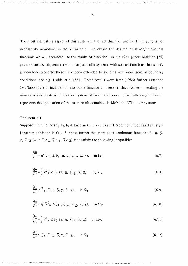
197

The most interesting aspect of this system is the fact that the function f1 (u , y , x) is not

necessarily monotone in the x variable. To obtain the des ired existence/uniqueness

theorems we will therefore use the results of McNabb. In his 1 96 1 paper, McNabb [55]

gave existence/uniqueness results for parabolic systems with source functions that satisfy

a monotone property, these have been extended to systems with more general boundary

condi tions, see e .g . Ladde et al [56] . These resul ts were later ( 1 986) further extended

(McNabb [57]) to include non-monotone functions. These results involve imbedding the

non-monotone system in another system of twice the order. The fol lowing Theorem

represents the application of the main result contained in McNabb 1 57 1 to our system :

Theorem 6.1

Suppose the functions f1 , f2, f3 defined in (6 . 1 ) - (6 .3) are Holder continuous and satisfy a

Lipschitz condition in QT· Suppose further that there exist continuous functions u , 1!, y,

�' x, x (with u 2 1!, y 2 �' x 2 x) that satisfy the following inequalities

CJU I n2- - --ar - 11 v u 2 F1 (u, 1!, y, y, x, x) ,

� 'Y n2- -

F (- ) d t - � v y 2 2 U , !J, y , �' X , X '

ax - _

Clt ;::: F3 (u , IJ, y, y,

CJ!J I 'V') -ar - 11 -u s; E1 cu,

dy 'Y � - - V2y < F cu d t E _

- -2 '

dX _ ()� � E3 (u , IJ, y, y,

X,

IJ,

1!,

-X ,

,�) , in QT,

- x), y, y, X,

y, y , X, x),

X) , in QT,

(6 .7)

(6 . 8 )

(6 .9 )

i n QT, (6 . 1 0)

in QT, ( 6 . 1 1 )

(6 . 1 2 )

where

au . _ .

U au

B ' -:� + B1 u 2:: B1 2:: ::'1- + 1 u , an un -

::'1- a l}j'_ > 0 > _r ::'I ll an - - an ' on U�l.T,

ax > 0 > ax on an-, an - - an '

"""'!'

u (r,O) 2:: � 1 (r) 2:: 1! (r,O), on Q,

y (r,O) 2:: \jf 1 (r) 2:: � (r,O) , on Q,

x (r,O) ;::: x 1 (r) ;::: X (r,O), on Q,

-F l (u, 1!, y, �' X , X) = sup

y ::; 92 ::; y _i::; e3 ::; X.

F2 (u, - - x) 1!, y, y, X , = sup

!! ::; e 1 ::; u ..::; ::; e3 ::; X.

F 3 cu, - - X) 1!, y, y, X = sup '

!! ::; 8 1 ::; u r ::; 92 ::; Y

1 98

f1 (u, 02, 03 ) ,

f2 (81 , y , 83) ,

f3 (8 1 , 82, x) ,

E 1 (u, .u., y, y, x, x) = inf f1 (1!, 82, 83) , -Y ::; e2 ::; Y � ::; e3 ::; X.

E2 (u, .u., y, �' x, x) = inf f2 (81 , �' 83) , !! ::; 91 ::; u _;:; ::; 93 ::; X.

(6 . 1 3)

(6 . 1 4)

(6 . 1 5 )

(6 . 1 6)

(6 . 17 )

(6 . 1 8 )

199

E3 (u, 11, y, �, x, x) = inf !! ::; e1 ::; ii � ::; ez ::; Y

Then there exis ts a unique solution u , y , x of (6. 1 ) - (6.6), (3 .35) - (3 . 37) with

Proof

See McNabb [55] , [ 571 ,

11

U sing the above Theorem leads to the main result of this chapter:

Theorem 6.2

The system (6. 1 ) - (6.6), (3 .35) - (3.37) has a u nique solution u, y , x satisfy ing

w h ere

w is the solution of (5 . 1 ) , (5 .2) ,

(6 . 1 9 )

200

(6 .20)

(6 . 2 1 )

(6 .22)

(6 .23)

(6.24)

Proof

It i s easy to show that the fi , i = 1 , 2, 3 sati sfy the desired Holder and Li p sch i tz

conditions, since the partia l derivatives of the fi with respect to u , y, x are bounded on any

bounded region (u 2 0), (for u = 0 we replace ex� -l�) etc . by zero) . So we must simply

find functions u, JJ., y, �' X:, x that satisfy the inequalities (6.7) - (6. 1 8) . Now reinforcing

i nequalities (6 .7) - (6. 1 2) gives

au I n2- '\ { - h -} at - 11 v U 2 1 + /\., hw <Pw X + c <Pc y , ( 6 .25)

(6 .26)

(6 .27)

dy y 2 1 �t

- - V Y � - - <l>c Y ' 0 E - E -

dX 1 --= < - rh X d t - -E

'l'c - .

201

(6 .28)

(6 .29)

(6 .30)

Clearly 11 = � = x = 0 satisfy the i nequal i ties (6 .28) - (6 .29) and the righ t-hand

inequalities of (6. 1 3) - (6. 1 8 ) . Now consider the functions x 1 , y 1 that satisfy the coupled

ordinary differential equations

This system has the simple analytic solution

where )l 1 , )l2, B 1 , A1 are as defined in (6. 1 9) - (6.22). I t is easy to show that B 1 > 0 and

A 1 can be positive or negative depending on the ini tial conditions . Further, y1 � l l\j1)10 for

all t > 0 and xl � I IX l l l o for all t > 0. Clearly y = Yl and X = xl satisfy the inequalities

202

(6.26) , (6 .27) and the left-hand inequal i ties of (6 . 1 4) , (6 . 1 5) , (6. 1 7 ) , (6. 1 8) . Next,

reinforcin g inequali ty (6.25) gives

au ' n2- c at - 11 v u ;?: 1 + D1 exp(�2 t) ,

where C1 , D 1 are as defined in (6.23), (6.24).

Now consider the function

this function satisfies

(6 .3 1 )

S o clearly u = u 1 satisfies (6.3 1 ) , as well as the left-hand i nequality of (6. 1 6) . Finally this

choice of u satisfies

au B · -::;- + l u un C1 + D1 exp(�2 t) Clw . ( r C 1 + 0 1 exp(�2 t) J =

11, � + B1 l l s 1 1 1 0 + U + 11 , w ,

203

so the left-hand inequal i ty of (6. 1 3) is satisfied also.

This completes the proof.

N o te :

11

The above resul ts a lso hold in the l imit ing case B i --7 oo , with the boundary

conditions for u and w given by (5 .4) and (5 .5) respectively, and a modified

boundary inequality (6. 1 3 ) of the form

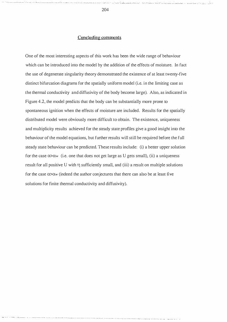
204

Concluding comments

One of the most interesting aspects of this work has been the wide range of behaviour

which can be introduced into the model by the addition of the effects of moisture. In fact

the use of degenerate singularity theory demonstrated the existence of at least twenty-five

distinct bifurcation diagrams for the spatially uniform model (i.e. i n the limiting case as

the thermal conductivity and diffusivity of the body become large). Also, as indicated in

Figure 4.2, the model predicts that the body can be substantially more prone to

spontaneous ignition when the effects of moisture are included . Results for the spatially

distributed model were obviously more difficult to obtain. The existence, uniqueness

and multiplicity results achieved for the steady state profiles give a good insight into the

behaviour of the model equations, but further results will still be required before the full

steady state behaviour can be predicted. These results include: (i) a better upper solution

for the case a>aw (i.e. one that does not get large as U gets small), (ii) a uniqueness

result for all positive U with 11 sufficiently small, and (iii) a result on multiple solutions

for the case a>aw (indeed the author conjectures that there can also be at least five

solutions for finite thermal conductivity and diffusivity).

205

References

1 1 j BOWES , P.C. S el f-heati ng: evaluating and con trol l ing the hazards. Elsevier, New

York. 1 984.

[2 J SEMENOV, N . N . Chemical k inetics and chain reactions . Oxford Univers i ty Press,

London. 1 935.

[ 3 ] FRANK-KAMENETSKII, D .A . Calculation o f thermal explosion l imits . Acta Phys. Chim. URSS 10 ( 1939), 365-370.

[ 4 ] ORA Y , P . , HARPER, M.J . Thermal explosions 1 : induction periods and temperature

changes before spontaneous ignition. Trans. Faraday Soc. 55 ( 1959), 5 8 1 -590.

[ 5 ] BODDINGTON, T. , GRAY, P . , HARVEY, D .I . Thermal theory of spontaneous igni tion: criticality i n bodies of arbitrary shape. Phil . Trans. Royal . Soc. A270 ( 1 97 1 ) , 467-506.

[ 6 ] BODDINGTON, T. , GRAY, P. , WAKE, G .C. Criteria for thermal explosions wi th and

without reactan t consumption. Proc. R. Soc. Lond . A357 ( 1977), 403-422.

[ 7 ] WAKE, G .C. Critical i ty with variable thermal conductiv i ty. Comb. Flame. 39 ( 1 980), 2 1 5-2 1 8 .

[ 8 ] THOMAS, P.H. , BOWES , P.C. Thermal ign ition i n a slab with one face at a constant high temperature. Trans. Faraday S oc. 57 ( 196 1 ) , 2007-201 7 .

l 9 J SHOUMANN , A.R., DONALDSON, A.B. The stationary problem of thermal i gnition in

a reactive slab with unsymmetric boundary temperatures. Combust. Flame 24

( 1975), 203-210 .

[ 1 0] S ISSON, R.A. , SWIFT, A . , WAKE, G .C. Spontaneous igni tion of materials on hot

surfaces. Math . Engng. I nd. 2 ( 1 990), 287-30 1 .

] 1 1 ] BURNELL, J .G . , LACEY, A .A . , WAKE, G .C. S teady states of the reaction d iffusion

equations. Part I : questions of existence and continu i ty of sol ution branches. J. Austral . Math . Soc. 24 ( 1 983) , 374-39 1 .

206

[ 1 2] BURNELL, J .G. , GRAHAM-EAGLE, J .G. , GRAY, B.F. , WAKE, G.C. Determin ation of critical ambient temperatures for thermal ignition. IMA J . App. Math. 42 ( 1 9 89),

147- 1 54.

[ 1 3 ] WAKE, G.C. , B URNELL, J .B . , GRAHAM-EAGLE, J .G. , GRAY, B .F. A new scaling of

a problem i n combustion theory. Proceedings of the Heriot-Watt S ymposium on Reaction-Diffu sion Equations, 25-37 . Clarendon Press, Oxford. 1990.

[ 1 4] GRAY, B .F . , GRIFFITHS , J .F. , HAS KO, S .M. Spontaneous ignition hazards i n stockpi les of cellulosic material s : criteria for safe s torage. J . Chem. Tech. Biotechnol . 34A ( 1984) , 453-463 .

[ 1 5 ] EGEIBAN, O.M. , GRIFFITHS, J .F. , MULLINS , J .R . , SCOTT, S .K. Explosion hazards in exothermic material s : critical conditions and scaling rules of masses of different goemetry. 19th Symp. (Int. ) Combustion. The Combustion Institute, 825 . 1 982.

[ 1 6] JONES , J .C . Determination of safe s tockpil ing practices for combustible sol ids by laboratory-scale tests. Chem. Engng. Austral . Ch E 1 3 No. 1 ( 1 988) , 9- 10 .

[ 1 7 ] JONES , J .C. The self-heating of wool and i t s conformity to ignition theory. Wool

Technology and Sheep Breeding. December 1 988 , 1 37- 14 1 .

[ 1 8 ] JONES, J .C. , RAJ, S .C. The self-heating and ignition of hops. J . Inst. Brew. 94 ( 1 988) , 139- 14 1 .

[ 1 9 ] JONES, J .C . , RAJ, S .C. The self-heating and ignition of vegetation debris . Fuel 67 ( 1 9 88), 1208- 12 10.

[ 20] RAJ, S .C. , JONES, J .C. Self-heating in the oxidation of natural materials from Fij i . NZ J.

Technology 3 ( 1989), 1 99-203.

[ 2 1 ] BOWES, P .C . , CAMERON, A . Self-heating and ignition of chemically activated carbon. J . Appl . Chem. B iotechnol. 21 ( 1 97 1 ) , 244-250.

[22] SMITH, R. S . Colonization and degradation of outside stored softwood chips by fungi. IUFRO S ymposium 1 972 Protection of Wood in S torage, XVI. Royal College of Forestry, S tockholm.

207

[23 ] DIXON, T.F. Spontaneous combustion in bagasse stockpiles. J . Fire Science. In press .

[24] GRAY, B .F . , S COTT, S .K. The influence of initial temperature-excess on critical

conditions for thermal explosion. Comb. Flame 61 ( 1 985) , 227 .

[25 ] HENRY, P .S .H. Diffusion in absorbing media. Proc. R . Soc. Lond. A 1 7 1 ( 19 39) , 2 1 5-241 .

[26 ] WALKER, I.K. , HARRISON, W.J. S elf heating of wet wood 1 : exothermic oxidation of wet sawdust. NZ. J. Science 20 ( 1 977), 1 9 1 -200.

[27] WALKER, I.K. , JACKSON, F.H. Changes of bound water in wood. NZ. J . Science 2 1 ( 1 978) , 32 1 -328.

[ 28 ] WALKER, I .K. , MANSSEN, N .B . Self-heating of wet wood 2: ignition by slow thermal explosion . NZ J. Science 22 ( 1 979), 99- 1 03 .

[29 ] GRAY, B .F. , WAKE, G.C. The ignition of hygroscopic materials by water. Comb. Flame 79 ( 1 990), 2-6.

[ 30] GRAY, B .F. Analysis of chemical kinetic systems over the entire parameter space Ill: a wet combustion system. Proc. R. Soc. Lond. A429 ( 1 990), 449-458.

[ 3 1 ] LADYZENSKAJA, O .A . , S OLONNIKOV, V.A. , URAL'CEV A, N.N. Linear and quasi l inear equation s of parabolic type. American Mathematica l S ociety

Translations of Mathematical Monographs 23. American Mathematica l Society, Providence, Rhode Island. 1 968 .

[ 3 2] SPERB , R . Maximum principles and their app lications. Mathematics i n S cience and

Engineering Vol. 1 57 . Academic Press. 1 98 1 .

[ 3 3 ] GILBARG, D . , TRUDINGER, N.S . E lliptic partial differen tial equations of second order. Springer-Verlag. 1 977.

[ 3 4] SATTINGER, D.H. Monotone methods in nonl inear elliptic and parabolic boundary value problems. Indiana University Mathematics Journal 2 1 No. 1 1 ( 1 972) , 979-1 000.

208

[ 3 5 ] AGMON, S . , DOUGLIS , A . , NIRENBERG, L. Estimates near the boundary for solutions of elliptic partial differential equations satisfying general boundary

conditions , I. Comm. Pure Appl . Math. 1 2 ( 1959), 623-727 .

[ 3 6] KEMPNER, E .S . Upper temperature limit of life. Science 142 ( 1 963), 1 3 1 8- 1 3 1 9.

[ 37 ] KELLER, H.B . , COHEN, D .S . Some positone problems suggested by nonlinear heat generation. J. Math. Mech. 1 6 No. 1 2 ( 1 967), 1 36 1 - 1 376.

[ 3 8 ] FRADKIN, L.J . , WAKE, G .C. Perturbations o f nonlinear eigenvalue problems. J . Math. Anal. Appl . Vol . 66 No. 2 ( 1978) , 433-44 1 .

[ 3 9 ] JONES, B . Personal communication. 1 990.

[ 40] SMEDLEY, S. Personal communication. 1 990.

[ 4 1 ] AB BOTT, J.P. An efficient algorithm for the determination of certain bifurcation points. J. Comput. App. Math . 4 ( 1 978) , 1 9-27.

[ 42] GRAY, B .F. , WAKE, G. C. On the determination of critical ambient temperatures and

critical initial conditions. Combust. Flame 17 ( 1988) , 1 0 1 - 1 04.

[ 43] D IEKMANN, 0 . , TEMME, N .M. Nonlinear diffusion processes. Math ematisch Centrum, Amsterdam. 1 976.

[ 44] STEGGERDA, J.J. Thermal stability : an extension of Frank-Kamenetskii 's t heory. J. Chem. Phy. 43 ( 1 965), 4446-4448 .

[ 45 ] ARIS , R. The mathematical theory of diffusion and reaction in permeable c atalysts, volume 1 : the theory of the steady state. Clarendon Press . Oxford. 197 5 .

[ 4 6 ] AMUNDSON, N.R. Mathematical models o f fixed bed reactors. Ber. (Otsch . ) B unsenges phys. Chem. 74 ( 1 970), 90.

[ 4 7 ] HEATH, J.M. The coupled diffusion of heat and moisture in bulk wool. PhD thesis. Victoria University of Wel lington. 1 982.

[ 48 ] GOLUBITSKY, M. , S CHAEFFER, D . S ingularities and groups in bifurcaticn theory, Vol. 1 . Appl . Math. Sciences 5 1 . Sp1inger Yerlag, New York. 1 985 .

209

[ 49] ORA Y, B .F. , ROBERTS , M.J . A method for the complete qualitative analysis of two

coupled ordinary differential equations dependent on three parameters. Proc. R .

Soc . Lond. A41 6 (198 8) , 3 6 1 -389.

[ 50 ] KELLER , H.B. Numerical solution of bifurcation and nonl inear eigenvalue problems. Applications of bifurcation theory (pp 359-384 ) . Academic Press. 1977 .

[ 5 1 ] RAY , W.H. B ifurcation phenomena in chemically reacting systems. Applications of bifurcation theory (pp 285-3 1 5) . Academic Press. 1977 .

[ 5 2 ] SEGEL, LA. Mathematical models in molecular and cellu lar biology. Cambridge

University Press. 1980.

[ 5 3 ] DA NCER , E .N. On the number of positive solution s of weak l y nonl inear ell iptic equations when a parameter is large. Proceedings of the London Mathematical Society 53 ( 1 9 8 6) , 429-452.

[ 54 ] FRIEDMAN, A . Partial differential equations. Bolt, Rinehart and Winston, New York .

1969 .

[ 5 5 ] McNA B B , A . Comparison and existence theorems for multicomponen t diffusion

systems. J . Math . Anal. Appl. 3 ( 1 96 1 ) , 1 33- 1 44.

[ 5 6 ] LADDE, G . S . , LA K SHMIKANTHAM, V . , VATSALA , A . S . Monotone i terat ive techn iques for n onlinear differential equations . Pitman, Boston . 1985 .

[ 5 7 ] McNAB B , A . Comparison theorems for differential equations. J . Math. Anal . Appl . 1 1 9

( 1986), 4 17-428 .

On mathematical modelling of the self-heating of ...

Documents

Transcript of On mathematical modelling of the self-heating of ...