on-line NotesBook Supplement - Ohio University4 1. Introduction 1.3 Vectors: Cartesian Re-Im...
117
on-line NotesBook Supplement
Transcript of on-line NotesBook Supplement - Ohio University4 1. Introduction 1.3 Vectors: Cartesian Re-Im...
on-line NotesBook Supplement
2
Mechanism Kinematics & Dynamics
Dr. Robert L. Williams II
Mechanical Engineering, Ohio University
NotesBook Supplement for ME 3011 Kinematics & Dynamics of Machines
© 2019 Dr. Bob Productions
ohio.edu/mechanical-faculty/williams
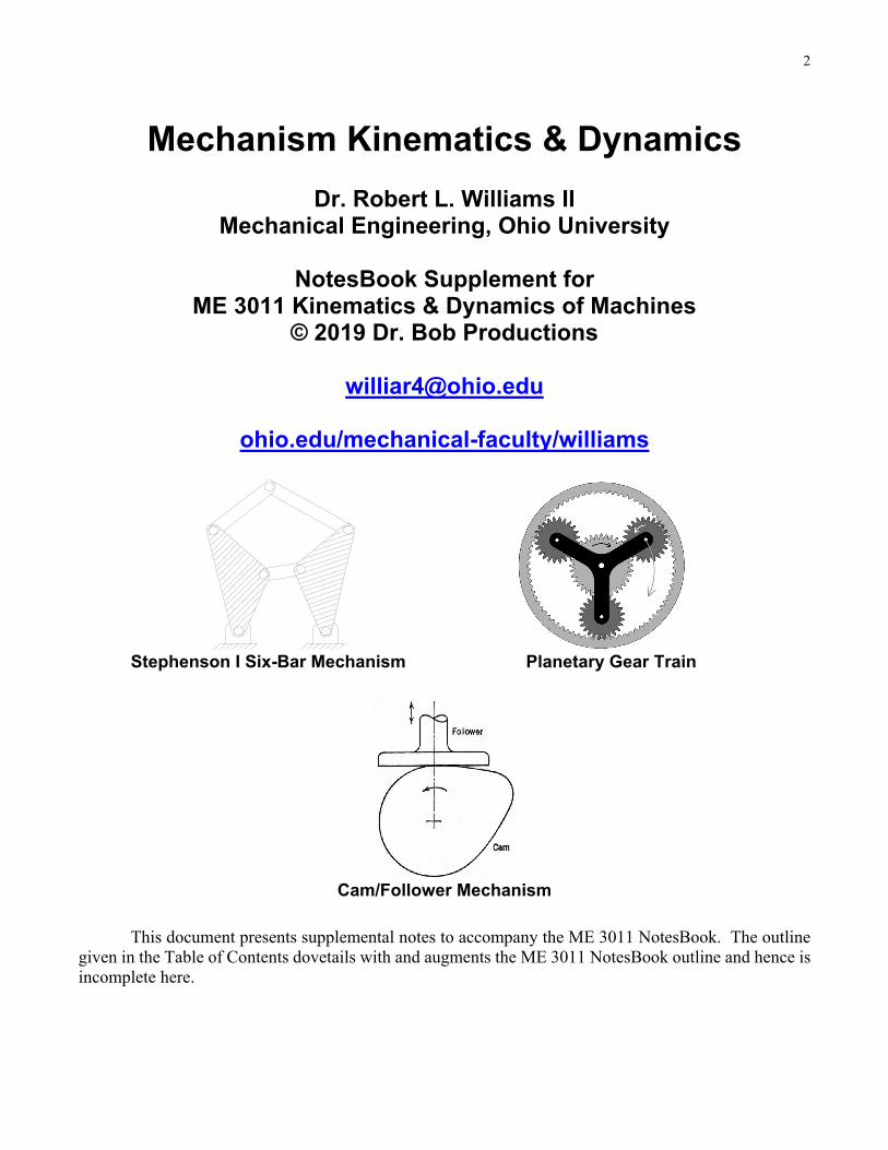
Stephenson I Six-Bar Mechanism Planetary Gear Train
Cam/Follower Mechanism
This document presents supplemental notes to accompany the ME 3011 NotesBook. The outline given in the Table of Contents dovetails with and augments the ME 3011 NotesBook outline and hence is incomplete here.
3
ME 3011 Supplement Table of Contents
1. INTRODUCTION................................................................................................................................ 4
1.3 VECTORS: CARTESIAN RE-IM REPRESENTATION (PHASORS) ....................................................... 4
2. POSITION KINEMATICS ANALYSIS............................................................................................ 6
2.1 FOUR-BAR MECHANISM POSITION ANALYSIS ................................................................................ 6 2.1.1 Tangent Half-Angle Substitution Derivation and Alternate Solution Method .................. 6 2.1.3 Four-Bar Mechanism Solution Irregularities ...................................................................... 12 2.1.4 Grashof’s Law and Four-Bar Mechanism Joint Limits ..................................................... 13
2.2 SLIDER-CRANK MECHANISM IRREGULAR DESIGNS ..................................................................... 22 2.3 INVERTED SLIDER-CRANK MECHANISM POSITION ANALYSIS ..................................................... 27 2.4 MULTI-LOOP MECHANISM POSITION ANALYSIS .......................................................................... 35
3. VELOCITY KINEMATICS ANALYSIS ........................................................................................ 39
3.1 VELOCITY ANALYSIS INTRODUCTION ........................................................................................... 39 Cyclist Zig-Zagging Uphill .............................................................................................................. 41
3.5 INVERTED SLIDER-CRANK MECHANISM VELOCITY ANALYSIS ................................................... 46 3.6 MULTI-LOOP MECHANISM VELOCITY ANALYSIS......................................................................... 50
4. ACCELERATION KINEMATICS ANALYSIS ............................................................................ 54
4.2 FIVE-PART ACCELERATION FORMULA ......................................................................................... 54 4.5 INVERTED SLIDER-CRANK MECHANISM ACCELERATION ANALYSIS .......................................... 55 4.6 MULTI-LOOP MECHANISM ACCELERATION ANALYSIS ................................................................ 61
5. OTHER KINEMATICS TOPICS .................................................................................................... 65
5.4 BRANCH SYMMETRY IN KINEMATICS ANALYSIS .......................................................................... 65 5.4.1 Four-Bar Mechanism ............................................................................................................. 65 5.4.2 Slider-Crank Mechanism ...................................................................................................... 67
6. INVERSE DYNAMICS ANALYSIS ............................................................................................... 69
6.1 DYNAMICS INTRODUCTION ............................................................................................................ 69 6.4 FOUR-BAR MECHANISM INVERSE DYNAMICS ANALYSIS ............................................................. 70 6.5 SLIDER-CRANK MECHANISM INVERSE DYNAMICS ANALYSIS ..................................................... 72 6.6 INVERTED SLIDER-CRANK MECHANISM INVERSE DYNAMICS ANALYSIS .................................... 74 6.7 MULTI-LOOP MECHANISM INVERSE DYNAMICS ANALYSIS ......................................................... 82 6.8 DYNAMIC BALANCING OF ROTATING SHAFTS .............................................................................. 87
7. GEARS AND CAMS ......................................................................................................................... 91
7.1 GEARS ............................................................................................................................................. 91 7.1.3 Gear Trains ............................................................................................................................. 91 7.1.4 Involute Spur Gear Standardization .................................................................................... 93 7.1.5 Planetary Gear Trains ......................................................................................................... 102
7.2 CAMS ............................................................................................................................................. 111 7.2.3 Analytical Cam Synthesis .................................................................................................... 111

4
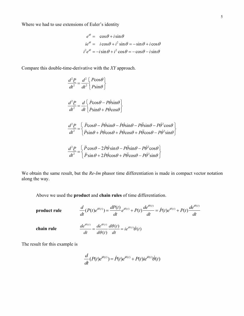
1. Introduction 1.3 Vectors: Cartesian Re-Im Representation (Phasors) Here is an alternate vector representation.
iP Pe The phasor iP e is a polar representation for vectors, where P is the length of vector P , e is the
natural logarithm base, 1i is the imaginary operator, and is the angle of vector P . ie gives the direction of the length P, according to Euler’s identity.
cos sinie i
ie is a unit vector in the direction of vector P . Phasor Re-Im representation of a vector is equivalent to Cartesian XY representation, where the real (Re)
axis is along X (or i ) and the imaginary (Im) axis is along Y (or j ).
cos(cos sin )
sin
cosˆ ˆ(cos sin )sin
Re i
Im
X
Y
P PP P i Pe
P P
P PP P i j
P P
A strength of Cartesian Re-Im representation using phasors is in taking time derivatives of vectors – the derivative of the exponential is easy ( ( )s sd ds e e ).
2 2
2 2
2
2
22 2
2
22
2
22
2
( )
2
cos 2 sin sin cos
sin 2 cos cos
i
i i
i i i i i
i i i i
d P d Pe
dt dt
d P dPe iP e
dt dt
d PPe iP e iP e iP e i P e
dt
d PPe iP e iP e P e
dt
P P P Pd P
dt P P P
2sinP
5
Where we had to use extensions of Euler’s identity
2
2 2
cos sin
cos sin sin cos
sin cos cos sin
i
i
i
e i
ie i i i
i e i i i
Compare this double-time-derivative with the XY approach.
2 2
2 2
2
2
22
2 2
2
2
cos
sin
cos sin
sin cos
cos sin sin sin cos
sin cos cos cos sin
cos 2 sin
Pd P d
Pdt dt
P Pd P d
dt dt P P
P P P P Pd P
dt P P P P P
P P Pd P
dt
2
2
sin cos
sin 2 cos cos sin
P
P P P P
We obtain the same result, but the Re-Im phasor time differentiation is made in compact vector notation along the way. Above we used the product and chain rules of time differentiation.
product rule ( ) ( )
( ) ( ) ( )( )( ( ) ) ( ) ( ) ( )
i t i ti t i t i td dP t de de
P t e e P t P t e P tdt dt dt dt
chain rule ( ) ( )
( )( )( )
( )
i t i ti tde de d t
ie tdt d t dt
The result for this example is
( ) ( ) ( )( ( ) ) ( ) ( ) ( )i t i t i tdP t e P t e P t ie t
dt
6
2. Position Kinematics Analysis 2.1 Four-Bar Mechanism Position Analysis
2.1.1 Tangent Half-Angle Substitution Derivation and Alternate Solution Method Tangent half-angle substitution derivation In this subsection we first derive the tangent half-angle substitution using an analytical/trigonometric method. Defining parameter t to be
tan2
t
i.e. the tangent of half of the unknown angle , we need to derive cos and sin as functions of parameter t. This derivation requires the trigonometric sum of angles formulae.
cos( ) cos cos sin sin
sin( ) sin cos cos sin
a b a b a b
a b a b a b
To derive the cos term as a function of t, we start with
cos cos2 2
The cosine sum of angles formula yields
2 2cos cos sin2 2
Multiplying by a ‘1’, i.e. 2cos2
over itself yields
2 2
2 2 2
2
cos sin2 2
cos cos 1 tan cos2 2 2cos
2
The cosine squared term can be divided by another ‘1’, i.e. 2 2cos sin 12 2
.
7
2
2
2 2
cos2
cos 1 tan2
cos sin2 2
Dividing top and bottom by 2cos2
yields
2
2
1cos 1 tan
21 tan
2
Remembering the earlier definition for t, this result is the first derivation we need, i.e.
2
2
1cos
1
t
t
To derive the sin term as a function of t, we start with
sin sin2 2
The sine sum of angles formula yields
sin sin cos cos sin 2sin cos2 2 2 2 2 2
Multiplying top and bottom by cosine yields
2 2
sin2
sin 2 cos 2 tan cos2 2 2cos
2
From the first derivation we learned
2
2
1cos
21 tan
2
8
Substituting this term yields
2
1sin 2 tan
21 tan
2
Remembering the earlier definition for t, this result is the second derivation we need, i.e.
2
2sin
1
t
t
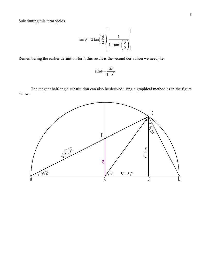
The tangent half-angle substitution can also be derived using a graphical method as in the figure below.
9
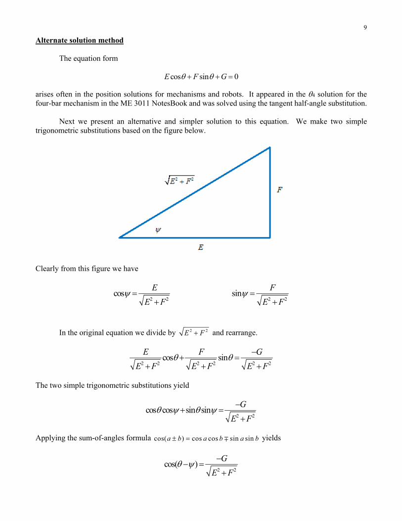
Alternate solution method The equation form
cos sin 0E F G
arises often in the position solutions for mechanisms and robots. It appeared in the 4 solution for the four-bar mechanism in the ME 3011 NotesBook and was solved using the tangent half-angle substitution. Next we present an alternative and simpler solution to this equation. We make two simple trigonometric substitutions based on the figure below.
Clearly from this figure we have
2 2cos
E
E F
2 2
sinF
E F
In the original equation we divide by 2 2E F and rearrange.
2 2 2 2 2 2cos sin
E F G
E F E F E F
The two simple trigonometric substitutions yield
2 2cos cos sin sin
G
E F
Applying the sum-of-angles formula cos( ) cos cos sin sina b a b a b yields
2 2cos( )
G
E F
10
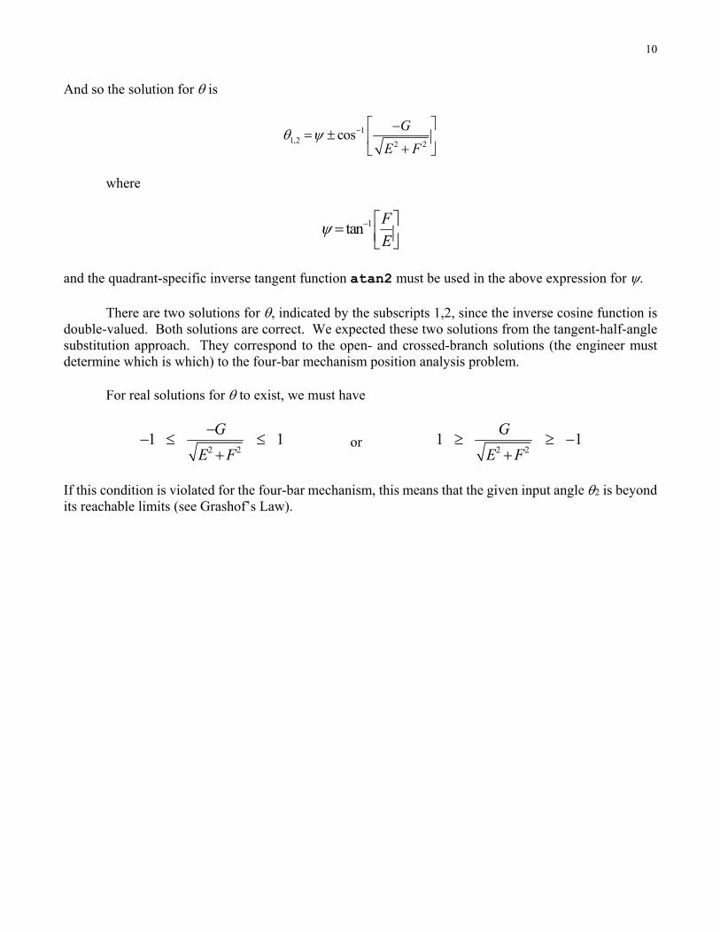
And so the solution for is
11,2 2 2
cosG
E F
where
1tanF
E
and the quadrant-specific inverse tangent function atan2 must be used in the above expression for . There are two solutions for , indicated by the subscripts 1,2, since the inverse cosine function is double-valued. Both solutions are correct. We expected these two solutions from the tangent-half-angle substitution approach. They correspond to the open- and crossed-branch solutions (the engineer must determine which is which) to the four-bar mechanism position analysis problem. For real solutions for to exist, we must have
2 21 1
G
E F
or
2 21 1
G
E F
If this condition is violated for the four-bar mechanism, this means that the given input angle 2 is beyond its reachable limits (see Grashof’s Law).
11
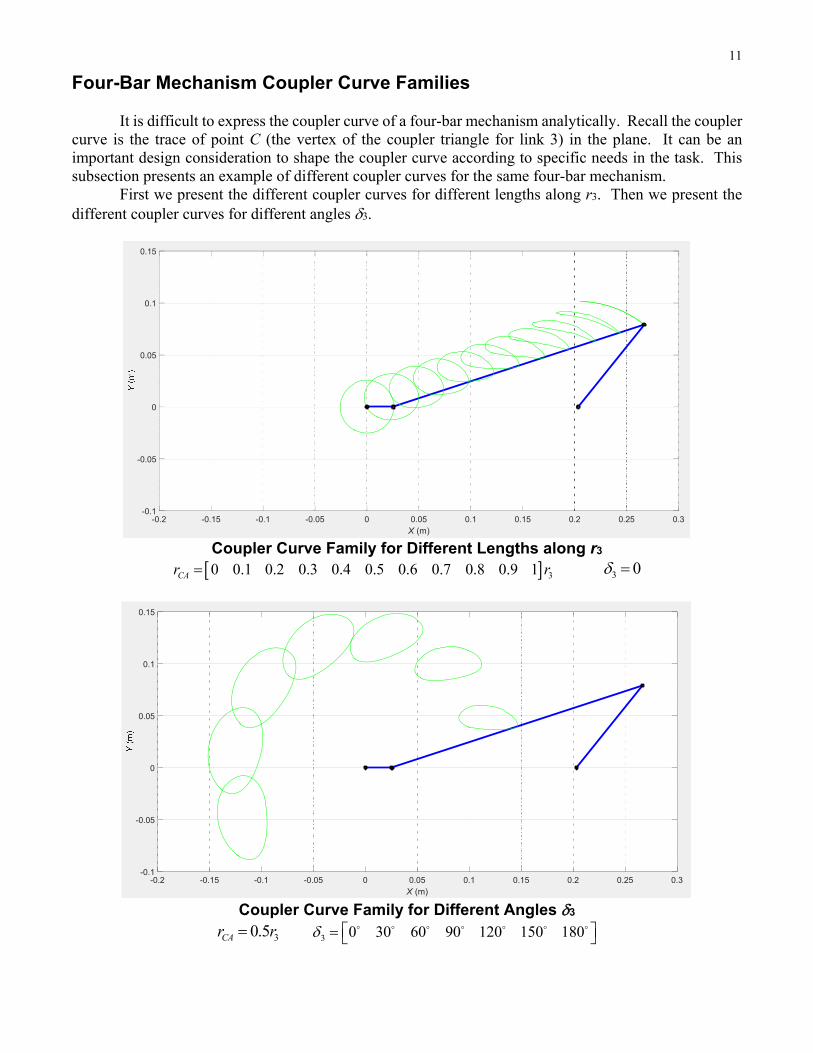
Four-Bar Mechanism Coupler Curve Families It is difficult to express the coupler curve of a four-bar mechanism analytically. Recall the coupler curve is the trace of point C (the vertex of the coupler triangle for link 3) in the plane. It can be an important design consideration to shape the coupler curve according to specific needs in the task. This subsection presents an example of different coupler curves for the same four-bar mechanism. First we present the different coupler curves for different lengths along r3. Then we present the different coupler curves for different angles 3.
Coupler Curve Family for Different Lengths along r3 30 0.1 0.2 0.3 0.4 0.5 0.6 0.7 0.8 0.9 1CAr r 3 0
Coupler Curve Family for Different Angles 3
30.5CAr r 3 0 30 60 90 120 150 180
-0.2 -0.15 -0.1 -0.05 0 0.05 0.1 0.15 0.2 0.25 0.3X (m)
-0.1
-0.05
0
0.05
0.1
0.15
-0.2 -0.15 -0.1 -0.05 0 0.05 0.1 0.15 0.2 0.25 0.3X (m)
-0.1
-0.05
0
0.05
0.1
0.15
12
2.1.3 Four-Bar Mechanism Solution Irregularities Four-bar mechanism position singularity 0G E
4 1 1 2 2
2 2 2 21 2 3 4 1 2 1 2
2 ( )
2 cos( )
E r rc r c
G r r r r r r
For simplicity, let 1 = 0 (just rotate the entire four-bar mechanism model for zero ground link angle).
2 2 2 21 2 3 4 1 4 2 4 1 22 2 ( ) 0G E r r r r r r r r r c
I have encountered two example four-bar mechanisms with this 0G E singularity. Case 1
When 1 4r r and 2 3r r , 2 2 2 2 21 2 2 1 1 2 1 1 22 2 ( ) 0G E r r r r r r r r c ALWAYS,
regardless of 2. Example
Given 1 2 3 410, 6, 6, 10r r r r ; this mechanism is ALWAYS singular. To fix this let
1 2 3 410, 5.9999, 6.0001, 10r r r r and MATLAB will be able to calculate the position analysis
reliably at every input angle. Case 2
When 1 32r r and 4 22r r , and furthermore 3 23 5r r ,
2 2 2 2
3 2 3 2 2 3 2 2 3 2
2 2 2 2 2 22 2 2 2 2 2 2
22 2
4 4 8 4 ( )c
100 25 40 84 c
9 9 3 38
c3
G E r r r r r r r r r
r r r r r r
r
This 0G E occurs only when 2 90 . Case 2 is much less general than case 1.
Example
Given 1 2 3 410, 3, 5, 6r r r r ; this mechanism is singular when 2 90 . To fix this ignore
2 90 or set your 2 array to avoid these values.
13
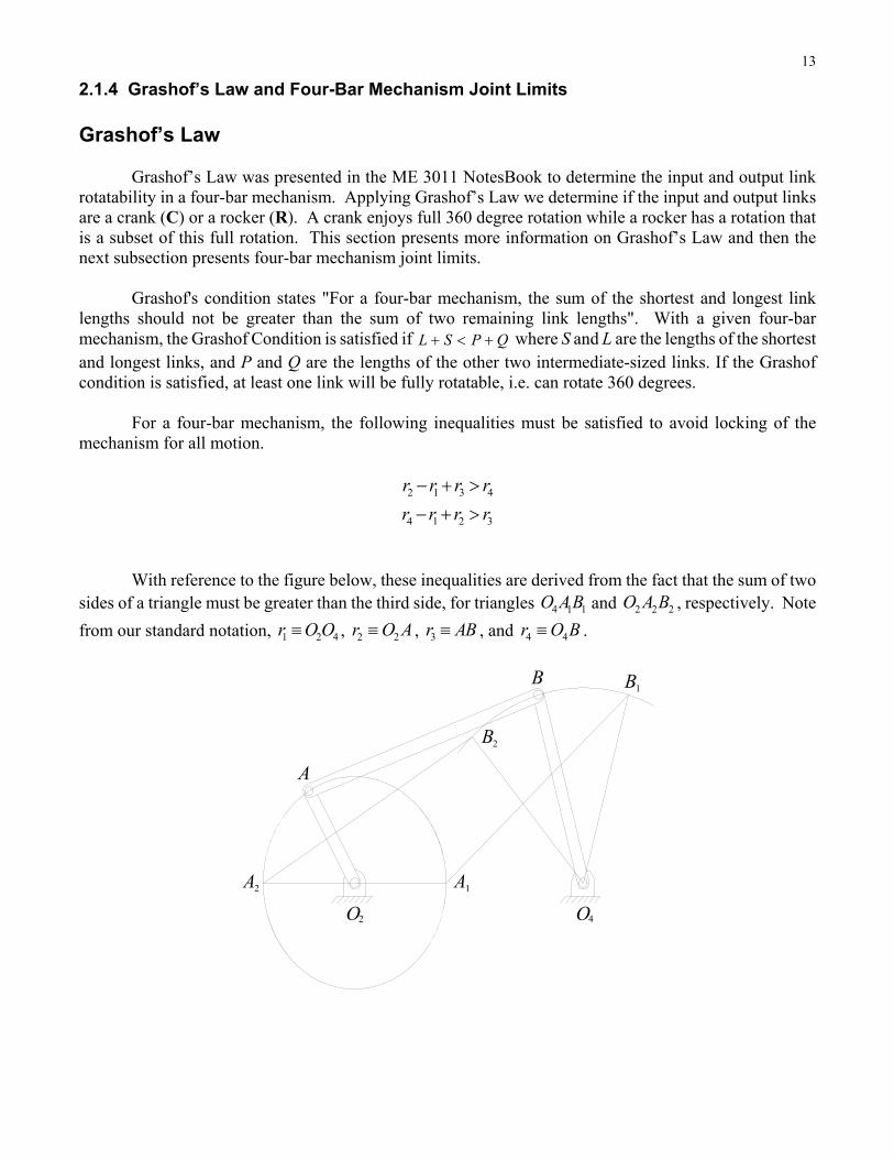
2.1.4 Grashof’s Law and Four-Bar Mechanism Joint Limits Grashof’s Law
Grashof’s Law was presented in the ME 3011 NotesBook to determine the input and output link rotatability in a four-bar mechanism. Applying Grashof’s Law we determine if the input and output links are a crank (C) or a rocker (R). A crank enjoys full 360 degree rotation while a rocker has a rotation that is a subset of this full rotation. This section presents more information on Grashof’s Law and then the next subsection presents four-bar mechanism joint limits.
Grashof's condition states "For a four-bar mechanism, the sum of the shortest and longest link lengths should not be greater than the sum of two remaining link lengths". With a given four-bar mechanism, the Grashof Condition is satisfied if L S P Q where S and L are the lengths of the shortest and longest links, and P and Q are the lengths of the other two intermediate-sized links. If the Grashof condition is satisfied, at least one link will be fully rotatable, i.e. can rotate 360 degrees.
For a four-bar mechanism, the following inequalities must be satisfied to avoid locking of the
mechanism for all motion.
2 1 3 4
4 1 2 3
r r r r
r r r r
With reference to the figure below, these inequalities are derived from the fact that the sum of two sides of a triangle must be greater than the third side, for triangles 4 1 1O AB and 2 2 2O A B , respectively. Note
from our standard notation, 1 2 4r O O , 2 2r O A , 3r AB , and 4 4r O B .
A
B
A
O
2
2 O4
A1
B1
B2
14
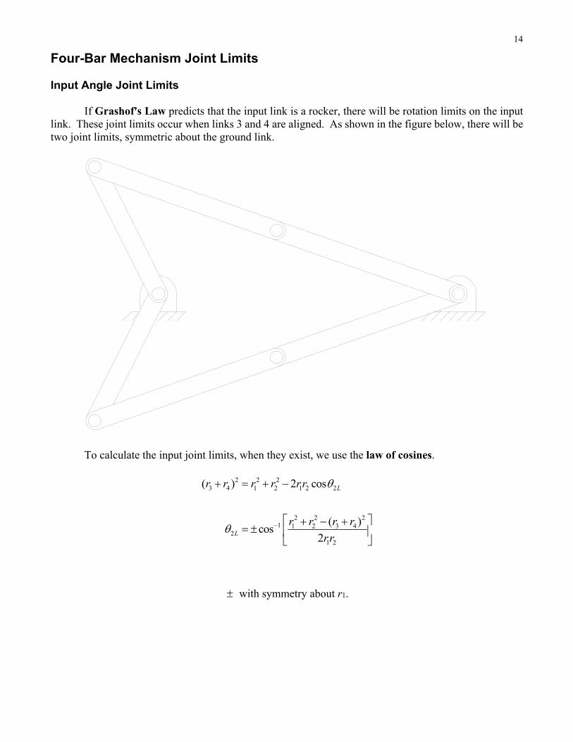
Four-Bar Mechanism Joint Limits Input Angle Joint Limits If Grashof's Law predicts that the input link is a rocker, there will be rotation limits on the input link. These joint limits occur when links 3 and 4 are aligned. As shown in the figure below, there will be two joint limits, symmetric about the ground link.
To calculate the input joint limits, when they exist, we use the law of cosines.
2 2 23 4 1 2 1 2 2
2 2 21 1 2 3 4
21 2
( ) 2 cos
( )cos
2
L
L
r r r r r r
r r r r
rr
with symmetry about r1.
15
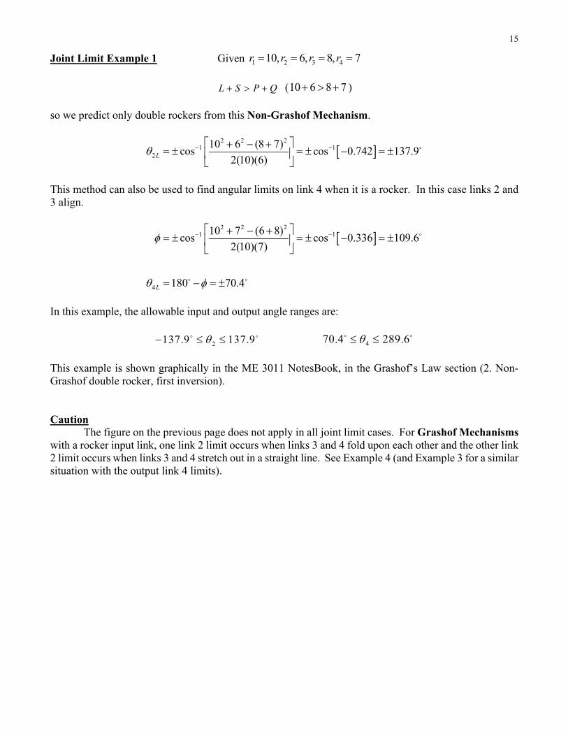
Joint Limit Example 1 Given 1 2 3 410, 6, 8, 7r r r r
L S P Q (10 6 8 7 )
so we predict only double rockers from this Non-Grashof Mechanism.
2 2 2
1 12
10 6 (8 7)cos cos 0.742 137.9
2(10)(6)L
This method can also be used to find angular limits on link 4 when it is a rocker. In this case links 2 and 3 align.
2 2 2
1 1
4
10 7 (6 8)cos cos 0.336 109.6
2(10)(7)
180 70.4L
In this example, the allowable input and output angle ranges are:
2137.9 137.9 470.4 289.6
This example is shown graphically in the ME 3011 NotesBook, in the Grashof’s Law section (2. Non-Grashof double rocker, first inversion).
Caution The figure on the previous page does not apply in all joint limit cases. For Grashof Mechanisms
with a rocker input link, one link 2 limit occurs when links 3 and 4 fold upon each other and the other link 2 limit occurs when links 3 and 4 stretch out in a straight line. See Example 4 (and Example 3 for a similar situation with the output link 4 limits).
16
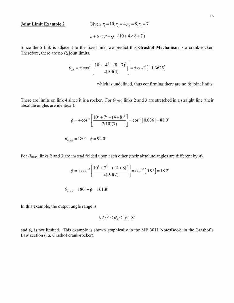
Joint Limit Example 2 Given 1 2 3 410, 4, 8, 7r r r r
L S P Q (10 4 8 7 )
Since the S link is adjacent to the fixed link, we predict this Grashof Mechanism is a crank-rocker. Therefore, there are no 2 joint limits.
2 2 2
1 12
10 4 (8 7)cos cos 1.3625
2(10)(4)L
which is undefined, thus confirming there are no 2 joint limits.
There are limits on link 4 since it is a rocker. For 4min, links 2 and 3 are stretched in a straight line (their absolute angles are identical).
2 2 2
1 1
4min
10 7 (4 8)cos cos 0.036 88.0
2(10)(7)
180 92.0
For 4max, links 2 and 3 are instead folded upon each other (their absolute angles are different by ).
2 2 2
1 1
4min
10 7 ( 4 8)cos cos 0.95 18.2
2(10)(7)
180 161.8
In this example, the output angle range is
492.0 161.8
and 2 is not limited. This example is shown graphically in the ME 3011 NotesBook, in the Grashof’s Law section (1a. Grashof crank-rocker).
17
Joint Limit Example 3 Given 1 2 3 411.18, 3, 8, 7r r r r (in) and 1 10.3
L S P Q (11.18 3 8 7 )
This is the four-bar mechanism from Term Example 1 and it is a four-bar crank-rocker Grashof Mechanism. There are no limits on 2 since link 2 is a crank. The 4 limits are
4 120.1L (links 2 and 3 stretched in a line)
4 172.5L (links 2 and 3 folded upon each other in a line)
The output angle range is
4120.1 172.5
and 2 is not limited. This example is NOT shown graphically in the ME 3011 NotesBook Grashof’s Law section. However, these 4 limits are clearly seen in the F.R.O.M. plot for angle 4 in Term Example 1 in the ME 3011 NotesBook.
18
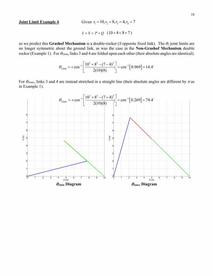
Joint Limit Example 4 Given 1 2 3 410, 8, 4, 7r r r r
L S P Q (10 4 8 7 )
so we predict this Grashof Mechanism is a double-rocker (S opposite fixed link). The 2 joint limits are no longer symmetric about the ground link, as was the case in the Non-Grashof Mechanism double rocker (Example 1). For 2min, links 3 and 4 are folded upon each other (their absolute angles are identical).
2 2 2
1 12min
10 8 (7 4)cos cos 0.969 14.4
2(10)(8)
For 2max, links 3 and 4 are instead stretched in a straight line (their absolute angles are different by as in Example 1).
2 2 2
1 12max
10 8 (7 4)cos cos 0.269 74.4
2(10)(8)
2min Diagram 2max Diagram
0 1 2 3 4 5 6 7 8 9 100
1
2
3
4
5
6
7
8
X (m)
Y (
m)
0 1 2 3 4 5 6 7 8 9 100
1
2
3
4
5
6
7
8
X (m)
Y (
m)

19
This behavior reverses for the 4 joint limits. For 4min, links 2 and 3 are stretched in a straight line (their absolute angles are identical).
2 2 2
1 1
4min
10 7 (8 4)cos cos 0.036 88.0
2(10)(7)
180 92.0
For 4max, links 2 and 3 are instead folded upon each other (their absolute angles are different by ).
2 2 2
1 1
4min
10 7 (8 4)cos cos 0.95 18.2
2(10)(7)
180 161.8
4min Diagram 4max Diagram
0 1 2 3 4 5 6 7 8 9 100
1
2
3
4
5
6
7
8
X (m)
Y (
m)
0 1 2 3 4 5 6 7 8 9 100
1
2
3
4
5
6
7
8
X (m)
Y (
m)
20
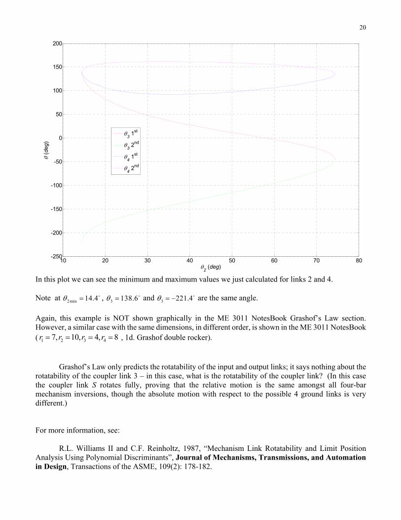
In this plot we can see the minimum and maximum values we just calculated for links 2 and 4. Note at 2 min 14.4 , 3 138.6 and 3 221.4 are the same angle.
Again, this example is NOT shown graphically in the ME 3011 NotesBook Grashof’s Law section. However, a similar case with the same dimensions, in different order, is shown in the ME 3011 NotesBook ( 1 2 3 47, 10, 4, 8r r r r , 1d. Grashof double rocker).
Grashof’s Law only predicts the rotatability of the input and output links; it says nothing about the rotatability of the coupler link 3 – in this case, what is the rotatability of the coupler link? (In this case the coupler link S rotates fully, proving that the relative motion is the same amongst all four-bar mechanism inversions, though the absolute motion with respect to the possible 4 ground links is very different.) For more information, see: R.L. Williams II and C.F. Reinholtz, 1987, “Mechanism Link Rotatability and Limit Position Analysis Using Polynomial Discriminants”, Journal of Mechanisms, Transmissions, and Automation in Design, Transactions of the ASME, 109(2): 178-182.
10 20 30 40 50 60 70 80-250
-200
-150
-100
-50
0
50
100
150
200
2 (deg)
(d
eg)
3 1st
3 2nd
4 1st
4 2nd
21
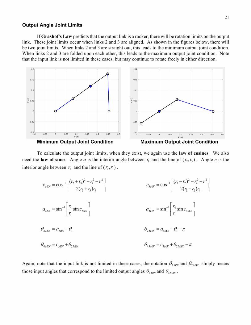
Output Angle Joint Limits If Grashof's Law predicts that the output link is a rocker, there will be rotation limits on the output link. These joint limits occur when links 2 and 3 are aligned. As shown in the figures below, there will be two joint limits. When links 2 and 3 are straight out, this leads to the minimum output joint condition. When links 2 and 3 are folded upon each other, this leads to the maximum output joint condition. Note that the input link is not limited in these cases, but may continue to rotate freely in either direction.
Minimum Output Joint Condition Maximum Output Joint Condition
To calculate the output joint limits, when they exist, we again use the law of cosines. We also need the law of sines. Angle a is the interior angle between 1r and the line of ( 2 3,r r ) . Angle c is the
interior angle between 4r and the line of ( 2 3,r r ) .
2 2 2
1 2 3 4 1
2 3 4
1 4
1
2 1
4 2
( )cos
2( )
sin sin
MIN
MIN MIN
MIN MIN
MIN MIN MIN
r r r rc
r r r
ra c
r
a
c
2 2 21 3 2 4 1
3 2 4
1 4
1
2 1
4 2
( )cos
2( )
sin sin
MAX
MAX MAX
MAX MAX
MAX MAX MAX
r r r rc
r r r
ra c
r
a
c
Again, note that the input link is not limited in these cases; the notation 2MIN and 2MAX simply means
those input angles that correspond to the limited output angles 4MIN and 4MAX .
22
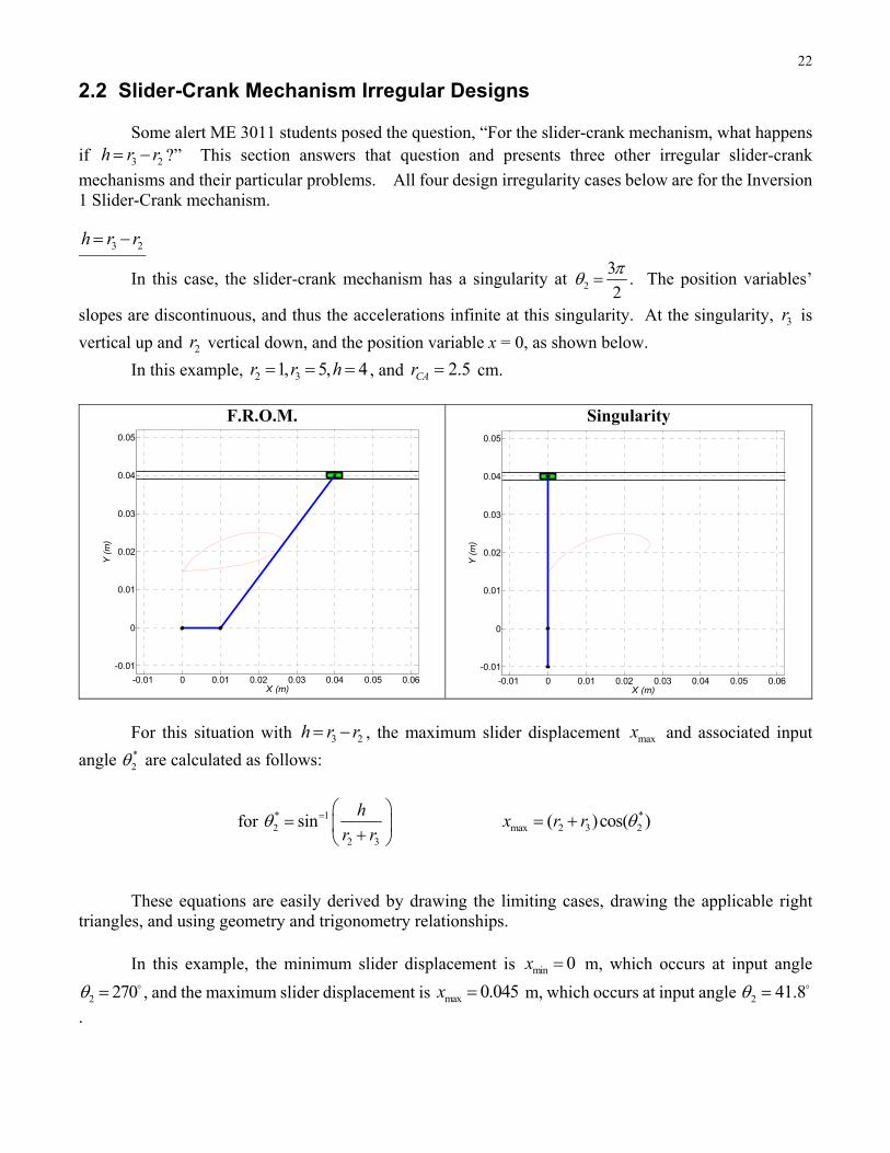
2.2 Slider-Crank Mechanism Irregular Designs Some alert ME 3011 students posed the question, “For the slider-crank mechanism, what happens if 3 2h r r ?” This section answers that question and presents three other irregular slider-crank
mechanisms and their particular problems. All four design irregularity cases below are for the Inversion 1 Slider-Crank mechanism.
3 2h r r
In this case, the slider-crank mechanism has a singularity at 2
3
2
. The position variables’
slopes are discontinuous, and thus the accelerations infinite at this singularity. At the singularity, 3r is
vertical up and 2r vertical down, and the position variable x = 0, as shown below.
In this example, 2 31, 5, 4r r h , and 2.5CAr cm.
F.R.O.M.
Singularity
For this situation with 3 2h r r , the maximum slider displacement maxx and associated input
angle *2 are calculated as follows:
for * 12
2 3
sinh
r r
*
max 2 3 2( )cos( )x r r
These equations are easily derived by drawing the limiting cases, drawing the applicable right triangles, and using geometry and trigonometry relationships.
In this example, the minimum slider displacement is min 0x m, which occurs at input angle
2 270 , and the maximum slider displacement is max 0.045x m, which occurs at input angle 2 41.8
.
-0.01 0 0.01 0.02 0.03 0.04 0.05 0.06
-0.01
0
0.01
0.02
0.03
0.04
0.05
X (m)
Y (
m)
-0.01 0 0.01 0.02 0.03 0.04 0.05 0.06
-0.01
0
0.01
0.02
0.03
0.04
0.05
X (m)
Y (
m)

23
2 3h r r
In this case, the slider-crank mechanism has a singularity at 2 2
. At the singularity, 3r is
vertical down and 2r is vertical up, and the position variable x = 0, as shown below. Also, the input angle
is limited (i.e. the ‘crank’ is not a crank). Further, unlike standard slider-crank mechanisms, this case has the possibility of branch-jumping (at the singularity), depending on mechanism links’ inertia. The condition for minimum input angle is when 2r and 3r are extended in a straight line. If the slider-crank
mechanism remains in the right branch, the condition for maximum input angle is when 2r and 3r are
perpendicular. The limit equations for this case are presented below. In this example, 2 35, 1, 4r r h , and 0.5CAr cm.
Minimum joint limit
Maximum joint limit
Singularity
-0.06 -0.04 -0.02 0 0.02 0.04 0.06-0.06
-0.04
-0.02
0
0.02
0.04
0.06
0.08
0.1
X (m)
Y (
m)
-0.06 -0.04 -0.02 0 0.02 0.04 0.06-0.06
-0.04
-0.02
0
0.02
0.04
0.06
0.08
0.1
X (m)
Y (
m)
-0.06 -0.04 -0.02 0 0.02 0.04 0.06-0.06
-0.04
-0.02
0
0.02
0.04
0.06
0.08
0.1
X (m)
Y (
m)
24
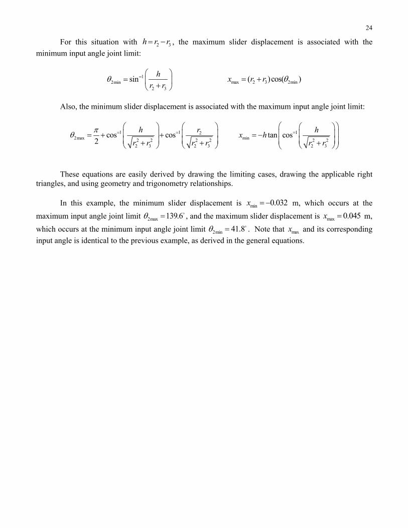
For this situation with 2 3h r r , the maximum slider displacement is associated with the
minimum input angle joint limit:
12min
2 3
sinh
r r
max 2 3 2min( )cos( )x r r
Also, the minimum slider displacement is associated with the maximum input angle joint limit:
1 1 22max 2 2 2 2
2 3 2 3
cos cos2
rh
r r r r
1min 2 2
2 3
tan cosh
x hr r
These equations are easily derived by drawing the limiting cases, drawing the applicable right triangles, and using geometry and trigonometry relationships.
In this example, the minimum slider displacement is min 0.032x m, which occurs at the
maximum input angle joint limit 2max 139.6 , and the maximum slider displacement is max 0.045x m,
which occurs at the minimum input angle joint limit 2min 41.8 . Note that maxx and its corresponding
input angle is identical to the previous example, as derived in the general equations.
25
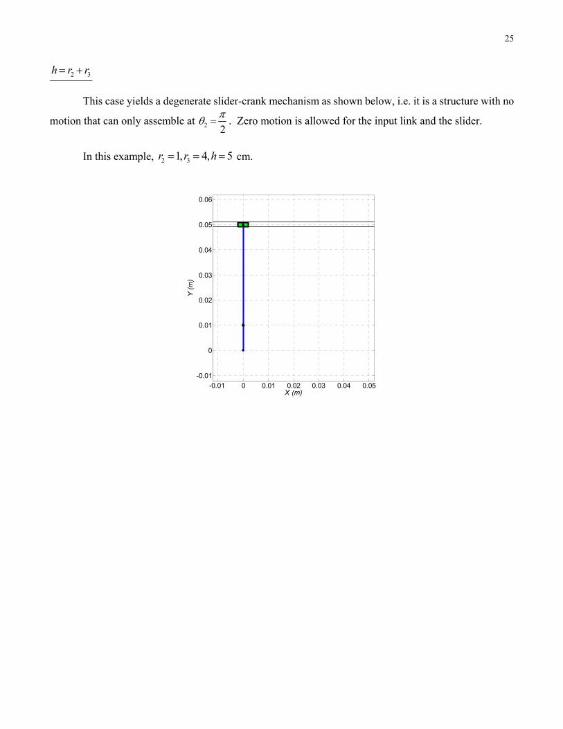
2 3h r r
This case yields a degenerate slider-crank mechanism as shown below, i.e. it is a structure with no
motion that can only assemble at 2 2
. Zero motion is allowed for the input link and the slider.
In this example, 2 31, 4, 5r r h cm.
-0.01 0 0.01 0.02 0.03 0.04 0.05
-0.01
0
0.01
0.02
0.03
0.04
0.05
0.06
X (m)
Y (
m)
26
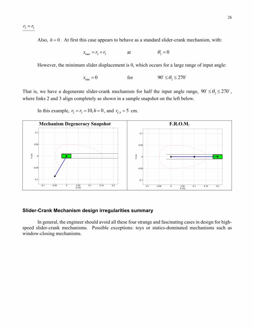
2 3r r
Also, 0h . At first this case appears to behave as a standard slider-crank mechanism, with:
max 2 3x r r at 2 0
However, the minimum slider displacement is 0, which occurs for a large range of input angle:
min 0x for 290 270
That is, we have a degenerate slider-crank mechanism for half the input angle range, 290 270 ,
where links 2 and 3 align completely as shown in a sample snapshot on the left below.
In this example, 2 3 10, 0r r h , and 5CAr cm.
Mechanism Degeneracy Snapshot
F.R.O.M.
Slider-Crank Mechanism design irregularities summary
In general, the engineer should avoid all these four strange and fascinating cases in design for high-speed slider-crank mechanisms. Possible exceptions: toys or statics-dominated mechanisms such as window-closing mechanisms.
-0.1 -0.05 0 0.05 0.1 0.15 0.2
-0.1
-0.05
0
0.05
0.1
X (m)
Y (
m)
-0.1 -0.05 0 0.05 0.1 0.15 0.2
-0.1
-0.05
0
0.05
0.1
X (m)
Y (
m)

27
2.3 Inverted Slider-Crank Mechanism Position Analysis This slider-crank mechanism inversion 2 is an inversion of the standard zero-offset slider-crank mechanism where the sliding direction is no longer the ground link, but along the rotating link 4. Ground link length r1 and input link length r2 are fixed; r4 is a variable. The slider link 3 is attached to the end of link 2 via an R joint and slides relative to link 4 via a P joint. This mechanism converts rotary input to linear motion and rotary motion output. Practical applications include certain doors/windows opening/damping mechanisms. The inverted slider-crank is also part of quick-return mechanisms. Step 1. Draw the Kinematic Diagram
r1 constant ground link length 2 variable input angle r2 constant input link length 4 variable output angle r4 variable output link length L4 constant total output link length Link 1 is the fixed ground link. Without loss of generality we may force the ground link to be horizontal. If it is not so in the real world, merely rotate the entire inverted slider-crank mechanism so it is horizontal. Both angles 2 and 4 are measured in a right-hand sense from the horizontal to the link. Step 2. State the Problem Given r1, 1 = 0, r2; plus 1-dof position input 2 Find r4 and 4

28
Step 3. Draw the Vector Diagram. Define all angles in a positive sense, measured with the right hand from the right horizontal to the link vector (tail-to-head; your right-hand thumb is located at the vector tail).
Step 4. Derive the Vector-Loop-Closure Equation. Starting at one point, add vectors tail-to-head until you reach a second point. Write the VLCE by starting and ending at the same points, but choosing a different path.
2 1 4r r r Step 5. Write the XY Components for the Vector-Loop-Closure Equation. Separate the one vector equation into its two X and Y scalar components.
2 2 1 4 4
2 2 4 4
r c r r c
r s r s
Step 6. Solve for the Unknowns from the XY equations. There are two coupled nonlinear equations in the two unknowns r4, 4. Unlike the standard slider-crank mechanism, there is no decoupling of X and Y. However, unlike the four-bar mechanism, there is only one unknown angle so the solution is easier than the four-bar mechanism. First rewrite the above XY equations to isolate the unknowns on one side.
4 4 2 2 1
4 4 2 2
r c r c r
r s r s
A ratio of the Y to X equations will cancel r4 and solve for 4.
4 4 2 2
4 4 2 2 1
r s r s
r c r c r
4 2 2 2 2 1a tan2( , )r s r c r
Then square and add the XY equations to eliminate 4 and solve for r4.
2 24 1 2 1 2 22r r r rr c
2
1
4

29
Note the same r4 formula results from the cosine law. Alternatively, the same r4 can be solved from either the X or Y equations after is 4 known.
X) 2 2 14
4
r c rr
c
Y) 2 2
44
r sr
s
Both of these r4 alternatives are valid; however, each is subject to a different artificial mathematical singularity ( 4 90 and 4 0,180 , respectively), so only the former square-root formula should be
used for r4, which has no artificial singularity. The X algorithmic singularity 4 90 never occurs unless
2 1r r , which is to be avoided (see below), but the Y algorithmic singularity occurs twice per full range
of motion.
Technically there are two solution sets – the one above and 2 2
4 1 2 1 2 22r r r rr c , 4 .
However, the negative r4 is not practical and so only the one solution set (branch) exists, unlike most planar mechanisms with two or more branches. Full-rotation condition For the inverted slider-crank mechanism to rotate fully, the fixed length of link 4, L4, must be greater than the maximum value of the variable r4. Slider Limits The slider reaches its minimum and maximum displacements when 2 = 0 and , respectively. Therefore, the slider limits are 1 2 4 1 2r r r r r . Thus, the fixed length L4 must be greater than 1 2r r .
In addition we require 1 2r r for full rotation.

30
Graphical Solution
The Inverted Slider-Crank mechanism position analysis may be solved graphically, by drawing the mechanism, determining the mechanism closure, and measuring the unknowns. This is an excellent method to validate your computer results at a given snapshot.
Draw the known ground link (points O2 and O4 separated by r1 at the fixed angle 1 = 0).
Draw the given input link length r2 at the given angle 2 (this defines point A).
Draw a line from O4 to point A.
Measure the unknown values of r4 and 4.
31
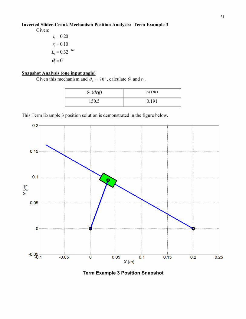
Inverted Slider-Crank Mechanism Position Analysis: Term Example 3 Given:
1
2
4
1
0.20
0.10
0.32
0
r
r
L
m
Snapshot Analysis (one input angle) Given this mechanism and 2 70 , calculate 4 and r4.
4 (deg) r4 (m)
150.5 0.191
This Term Example 3 position solution is demonstrated in the figure below.
Term Example 3 Position Snapshot
32
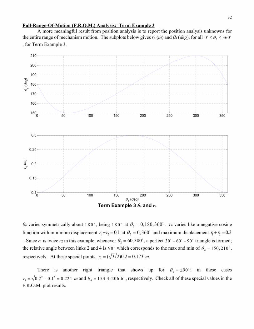
Full-Range-Of-Motion (F.R.O.M.) Analysis: Term Example 3 A more meaningful result from position analysis is to report the position analysis unknowns for the entire range of mechanism motion. The subplots below gives r4 (m) and 4 (deg), for all 20 360
, for Term Example 3.
Term Example 3 4 and r4
4 varies symmetrically about 1 8 0 , being 1 8 0 at 2 0,180,360 . r4 varies like a negative cosine
function with minimum displacement 1 2 0.1r r at 2 0,360 and maximum displacement 1 2 0.3r r
. Since r1 is twice r2 in this example, whenever 2 60,300 , a perfect 30 60 90 triangle is formed;
the relative angle between links 2 and 4 is 90 which corresponds to the max and min of 4 150, 210 ,
respectively. At these special points, 4 ( 3 2)0.2 0.173r m.
There is another right triangle that shows up for 2 90 ; in these cases
2 24 0.2 0.1 0.224r m and 4 153.4, 206.6 , respectively. Check all of these special values in the
F.R.O.M. plot results.
0 50 100 150 200 250 300 350150
160
170
180
190
200
210
4 (
deg)
0 50 100 150 200 250 300 3500.1
0.15
0.2
0.25
0.3
2 (deg)
r 4 (
m)
33
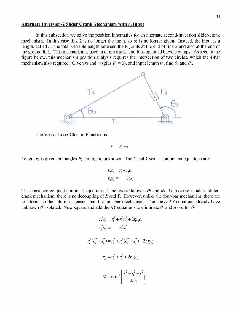
Alternate Inversion-2 Slider Crank Mechanism with r3 Input In this subsection we solve the position kinematics for an alternate second-inversion slider-crank mechanism. In this case link 2 is no longer the input, so 2 is no longer given. Instead, the input is a length, called r3, the total variable length between the R joints at the end of link 2 and also at the end of the ground link. This mechanism is used in dump trucks and foot-operated bicycle pumps. As seen in the figure below, this mechanism position analysis requires the intersection of two circles, which the 4-bar mechanism also required. Given r1 and r2 (plus 1 = 0), and input length r3, find 2 and 3.
The Vector Loop-Closure Equation is:
2 1 3r r r Length r3 is given, but angles 2 and 3 are unknown. The X and Y scalar component equations are:
2 2 1 3 3
2 2 3 3
r c r r c
r s r s
These are two coupled nonlinear equations in the two unknowns 2 and 3. Unlike the standard slider-crank mechanism, there is no decoupling of X and Y. However, unlike the four-bar mechanism, there are less terms so the solution is easier than the four-bar mechanism. The above XY equations already have unknown 2 isolated. Now square and add the XY equations to eliminate 2 and solve for 3.
2 2 2 2 22 2 1 3 3 1 3 3
2 2 2 22 2 3 3
2r c r r c rr c
r s r s
2 2 2 2 2 2 2
2 2 2 1 3 3 3 1 3 3
2 2 22 1 3 1 3 3
2 2 21 2 1 3
31 3
( ) ( ) 2
2
cos2
r c s r r c s rr c
r r r rr c
r r r
rr
34
What about trigonometric uncertainty? These mechanisms are generally designed to work only in one branch, often the + one; so just take the primary inverse cosine solution and the secondary one (negative) will not be admissible. To finish the solution,
1 3 32
2
sinr s
r
where we must substitute the value of 3 solved above. Again, trigonometric uncertainty is not a problem; just take the primary inverse sine solution. Certainly, you should validate the correct branch is obtained by a graphical solution.
35
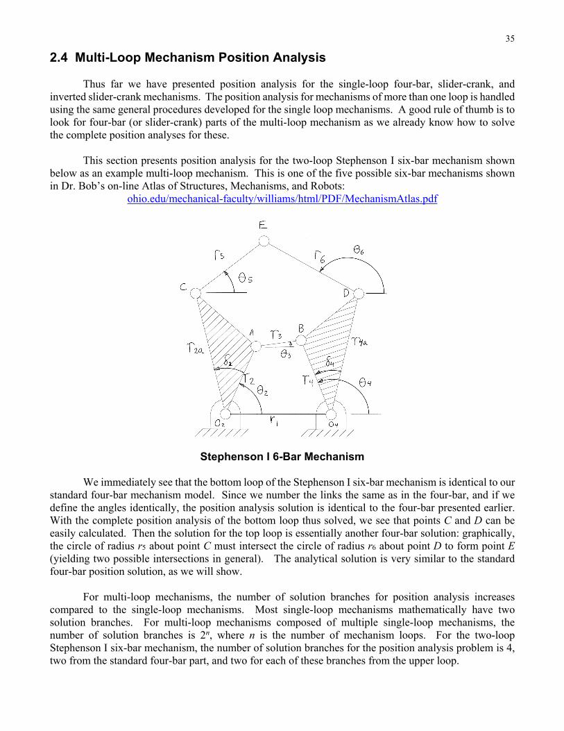
2.4 Multi-Loop Mechanism Position Analysis Thus far we have presented position analysis for the single-loop four-bar, slider-crank, and inverted slider-crank mechanisms. The position analysis for mechanisms of more than one loop is handled using the same general procedures developed for the single loop mechanisms. A good rule of thumb is to look for four-bar (or slider-crank) parts of the multi-loop mechanism as we already know how to solve the complete position analyses for these. This section presents position analysis for the two-loop Stephenson I six-bar mechanism shown below as an example multi-loop mechanism. This is one of the five possible six-bar mechanisms shown in Dr. Bob’s on-line Atlas of Structures, Mechanisms, and Robots:
ohio.edu/mechanical-faculty/williams/html/PDF/MechanismAtlas.pdf
Stephenson I 6-Bar Mechanism We immediately see that the bottom loop of the Stephenson I six-bar mechanism is identical to our standard four-bar mechanism model. Since we number the links the same as in the four-bar, and if we define the angles identically, the position analysis solution is identical to the four-bar presented earlier. With the complete position analysis of the bottom loop thus solved, we see that points C and D can be easily calculated. Then the solution for the top loop is essentially another four-bar solution: graphically, the circle of radius r5 about point C must intersect the circle of radius r6 about point D to form point E (yielding two possible intersections in general). The analytical solution is very similar to the standard four-bar position solution, as we will show. For multi-loop mechanisms, the number of solution branches for position analysis increases compared to the single-loop mechanisms. Most single-loop mechanisms mathematically have two solution branches. For multi-loop mechanisms composed of multiple single-loop mechanisms, the number of solution branches is 2n, where n is the number of mechanism loops. For the two-loop Stephenson I six-bar mechanism, the number of solution branches for the position analysis problem is 4, two from the standard four-bar part, and two for each of these branches from the upper loop.

36
Now let us solve the position analysis problem for the two-loop Stephenson I six-bar mechanism using the formal position analysis steps presented earlier. Assume link 2 is the input link. Step 1. Draw the Kinematic Diagram this is done in the figure above.
r1 constant ground link length 1 constant ground link angle r2 constant input link length to point A 2 variable input link angle r2a constant input link length to point C 2 constant angle on link 2 r3 constant coupler link length, loop I 3 variable coupler link angle, loop I r4 constant output link length, loop I 4 variable output link angle, loop I r4a constant input link length to point D 4 constant angle on link 4 r5 constant coupler link length, loop II 5 variable coupler link angle, loop II r6 constant output link length, loop II 6 variable output link angle, loop II As usual, all angles are measured in a right-hand sense from the absolute horizontal to the link, as shown in the kinematic diagram. Step 2. State the Problem Given r1, 1, r2, r3, r4, r2a, r4a, r5, r6, 2, 4; plus 1-dof position input 2 Find 3, 4, 5, 6 Step 3. Draw the Vector Diagram. Define all angles in a positive sense, measured with the right hand from the right horizontal to the link vector (tail-to-head with the right-hand thumb at the vector tail and right-hand fingers towards the arrow in the vector diagram below).
37
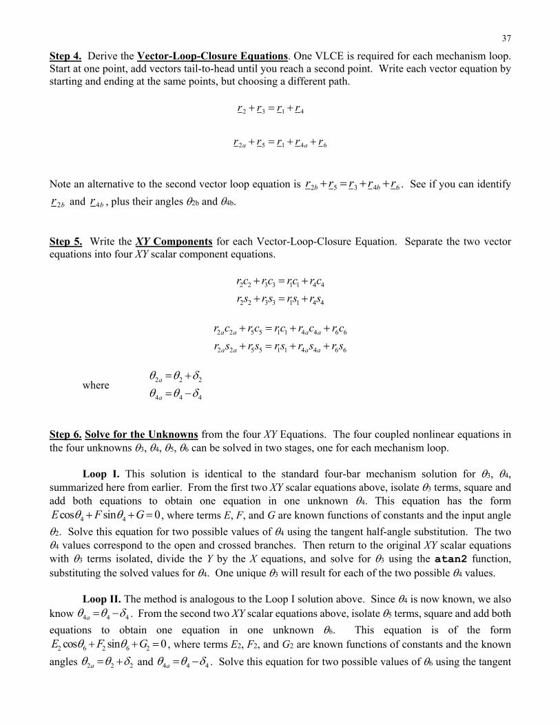
Step 4. Derive the Vector-Loop-Closure Equations. One VLCE is required for each mechanism loop. Start at one point, add vectors tail-to-head until you reach a second point. Write each vector equation by starting and ending at the same points, but choosing a different path.
2 3 1 4
2 5 1 4 6a a
r r r r
r r r r r
Note an alternative to the second vector loop equation is 2 5 3 4 6b br r r r r . See if you can identify
2br and 4br , plus their angles 2b and 4b. Step 5. Write the XY Components for each Vector-Loop-Closure Equation. Separate the two vector equations into four XY scalar component equations.
2 2 3 3 1 1 4 4
2 2 3 3 1 1 4 4
r c r c rc r c
r s r s rs r s
2 2 5 5 1 1 4 4 6 6
2 2 5 5 1 1 4 4 6 6
a a a a
a a a a
r c r c rc r c r c
r s r s r s r s r s
where 2 2 2
4 4 4
a
a
Step 6. Solve for the Unknowns from the four XY Equations. The four coupled nonlinear equations in the four unknowns 3, 4, 5, 6 can be solved in two stages, one for each mechanism loop.
Loop I. This solution is identical to the standard four-bar mechanism solution for 3, 4, summarized here from earlier. From the first two XY scalar equations above, isolate 3 terms, square and add both equations to obtain one equation in one unknown 4. This equation has the form
4 4cos sin 0E F G , where terms E, F, and G are known functions of constants and the input angle
2. Solve this equation for two possible values of 4 using the tangent half-angle substitution. The two 4 values correspond to the open and crossed branches. Then return to the original XY scalar equations with 3 terms isolated, divide the Y by the X equations, and solve for 3 using the atan2 function, substituting the solved values for 4. One unique 3 will result for each of the two possible 4 values.
Loop II. The method is analogous to the Loop I solution above. Since 4 is now known, we also know 4 4 4a . From the second two XY scalar equations above, isolate 5 terms, square and add both
equations to obtain one equation in one unknown 6. This equation is of the form
2 6 2 6 2cos sin 0E F G , where terms E2, F2, and G2 are known functions of constants and the known
angles 2 2 2a and 4 4 4a . Solve this equation for two possible values of 6 using the tangent
38
half-angle substitution. The two 6 values correspond to open and crossed branches, for each of the Loop I open and crossed branches. Then return to the original XY scalar equations with 5 terms isolated, divide the Y by the X equations, and solve for 5 using the atan2 function, substituting the solved values for 6. One unique 5 will result for each of the two possible 6 values from each 4.
Branches. There are two 5, 6 branches for each of the two 3, 4 branches, so there are four overall mechanism branches for the two-loop Stephenson I six-bar mechanism. Full-rotation condition The range of motion of a multi-loop mechanism may be more limited than that of single-loop mechanisms. One can perform a compound Grashof analysis when four-bars are the component mechanisms. For the two-loop Stephenson I six-bar mechanism, the second loop may constrain the first loop (e.g. it may change an expected crank motion of the input link to a rocker). This is an important issue in design of multi-loop mechanisms if the input link must still rotate fully. Graphical Solution The two-loop Stephenson I six-bar mechanism position analysis may readily be solved graphically, by drawing the mechanism, determining the mechanism closure, and measuring the unknowns. This is an excellent method to validate your computer results at a given snapshot. Loop I (this part is identical to the standard four-bar graphical solution)
Draw the known ground link (points O2 and O4 separated by r1 at the fixed angle 1). Draw the given input link length r2 at the given angle 2 to yield point A. Draw a circle of radius r3, centered at point A. Draw a circle of radius r4, centered at point O4. These circles intersect in general in two places to yield two possible points B. Connect the two branches and measure the unknown angles 3 and 4.
Loop II (this part is a modification of the standard four-bar graphical solution). Start with the end of the procedure above, on the same drawing. For each solution branch above, perform the following steps.
Draw the link r2a at angle 2 2 2a from point O2.
Draw the link r4a at angle 4 4 4a from point O4.
Draw a circle of radius r5, centered at point C. Draw a circle of radius r6, centered at point D. These circles intersect in general in two places to yield two possible points E. Connect the two branches and measure the unknown values 5 and 6.
In general, there are four overall position solution branches.
39
3. Velocity Kinematics Analysis 3.1 Velocity Analysis Introduction Here are a couple of fun scalar velocity problems involving average speed, time, and distance to get started with.
1. A cyclist travels uphill at a constant speed of 20 kph for 30 min; then the cyclist travels downhill at a constant speed of 60 kph for the next 30 min. What is the cyclist’s average speed for this motion?
Solution:
uphill: 20kph 0.5hr 10 km
downhill: 60kph 0.5hr 30km
total: 40km 1hr 40kph This answer is obvious, no? (i.e. the simple average of 20 and 60 kph) But how does the problem change if the distances are the same for both portions of the motion, rather than the times being the same as above?
2. A cyclist travels uphill at a constant speed of 20 kph for 10 km; then the cyclist travels downhill at a constant speed of 60 kph for the next 10 km. What is the cyclist’s average speed for this motion?
Solution:
uphill: hr 1
10 km hr20 km 2
downhill: hr 1
10 km hr60 km 6
total: 2
20 km hr 30 kph3
So the cyclist travels slower than the simple average when the distances are the same for both portions of the motion, rather than the times being the same. This phenomenon is called the Harmonic Mean of Velocity. The Harmonic Mean of a set of numbers is the inverse of the simple average of the inverse numbers of that set. For our second example, if a distance is covered at speed 1v and the same distance
is then covered at speed 2v , the Harmonic Mean applies to calculate average speed:
1 2
1 1 1avg
n
nv
v v v
1 2
1 2
1 2
221 1avg
v vv
v vv v
For the numerical example: 2(20)(60)
30 kph20 60avgv
40
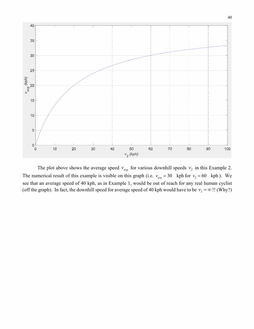
The plot above shows the average speed avgv for various downhill speeds 2v in this Example 2.
The numerical result of this example is visible on this graph (i.e. 30 kphavgv for 2 60 kphv ). We
see that an average speed of 40 kph, as in Example 1, would be out of reach for any real human cyclist (off the graph). In fact, the downhill speed for average speed of 40 kph would have to be 2v !! (Why?)
v avg (
kph)
41
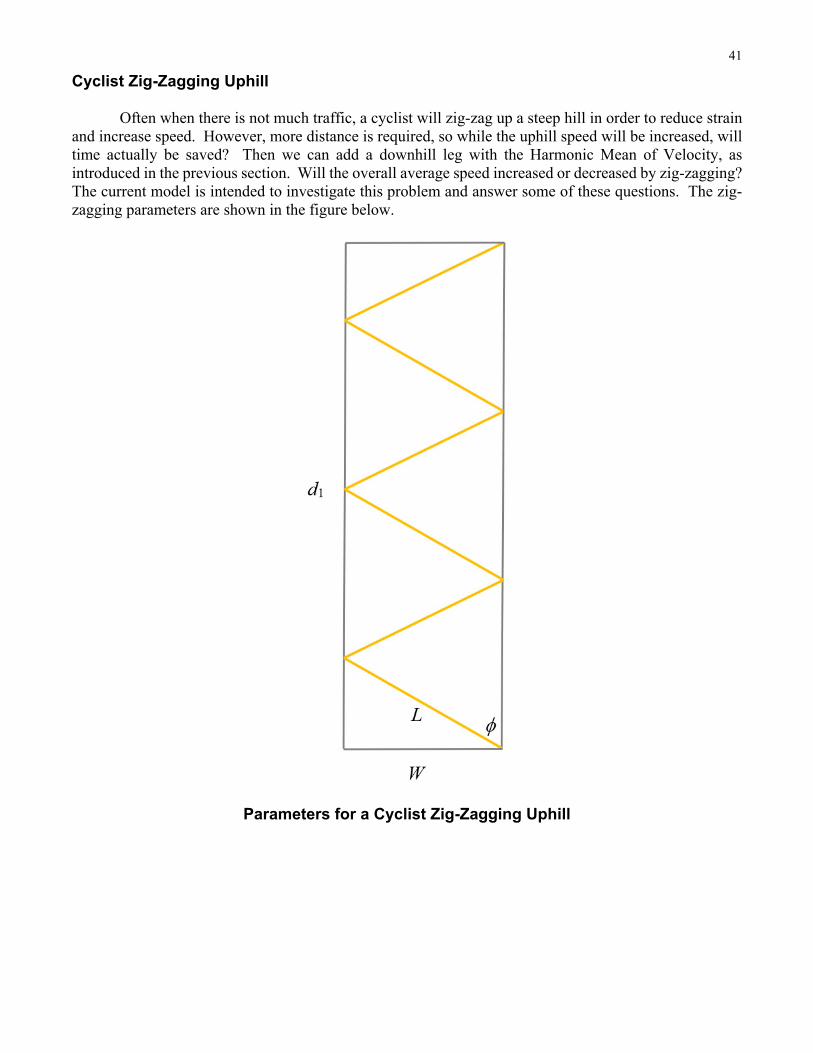
Cyclist Zig-Zagging Uphill Often when there is not much traffic, a cyclist will zig-zag up a steep hill in order to reduce strain and increase speed. However, more distance is required, so while the uphill speed will be increased, will time actually be saved? Then we can add a downhill leg with the Harmonic Mean of Velocity, as introduced in the previous section. Will the overall average speed increased or decreased by zig-zagging? The current model is intended to investigate this problem and answer some of these questions. The zig-zagging parameters are shown in the figure below.
Parameters for a Cyclist Zig-Zagging Uphill
42
Assumptions and relationships:
The hill has a constant uphill grade. The road is perfectly straight. The road is a standard 2-lane highway with a width of 8W m. The distance travelled on one zig or zag across the road is L. The uphill distance is 1 1 kmd . The total distance travelled while zig-zagging is
*1 12d NL d . The distance travelled straight along the road on one zig-zag is
1 1D d N .
The cyclist maintains a constant uphill speed 1v (despite continually turning sharp
corners!). There are no interruptions due to pesky traffic. The cyclist must divide the hill into a perfect N sections for zig-zagging.
1v represents the straight-uphill speed and *1v represents the uphill speed with zig-
zagging. *1 1v v
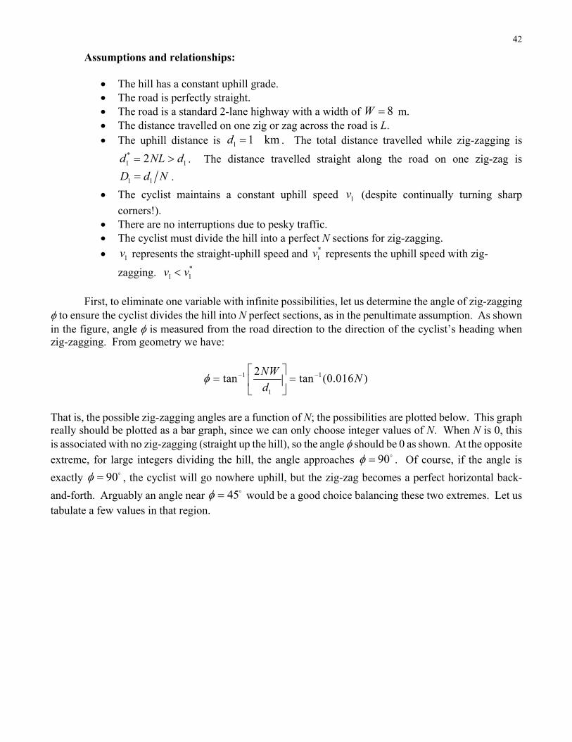
First, to eliminate one variable with infinite possibilities, let us determine the angle of zig-zagging
to ensure the cyclist divides the hill into N perfect sections, as in the penultimate assumption. As shown in the figure, angle is measured from the road direction to the direction of the cyclist’s heading when zig-zagging. From geometry we have:
1 1
1
2tan tan (0.016 )
NWN
d
That is, the possible zig-zagging angles are a function of N; the possibilities are plotted below. This graph really should be plotted as a bar graph, since we can only choose integer values of N. When N is 0, this is associated with no zig-zagging (straight up the hill), so the angle should be 0 as shown. At the opposite
extreme, for large integers dividing the hill, the angle approaches 90 . Of course, if the angle is
exactly 90 , the cyclist will go nowhere uphill, but the zig-zag becomes a perfect horizontal back-
and-forth. Arguably an angle near 45 would be a good choice balancing these two extremes. Let us tabulate a few values in that region.

43
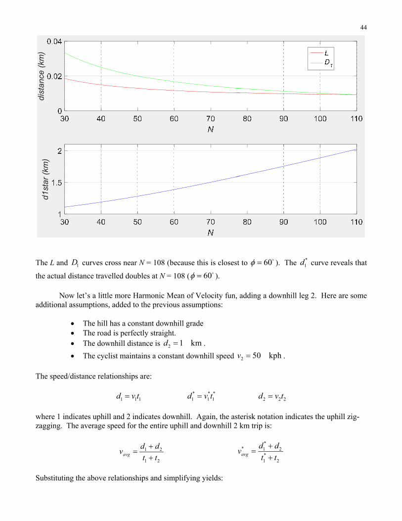
N 61 44.3 62 44.8 63 45.2 64 45.7
For further study in this problem, let us use:
N 36 29.9 62 44.8 108 59.9
Why? No special reason, other than the human need to force nice angles (essentially 30 ,45 ,60 ). The
plots below show some of the other important kinematic parameters ( *1 1, ,L D d ), in this zone of interest.
(de
g)
44
The L and 1D curves cross near N = 108 (because this is closest to 60 ). The *1d curve reveals that
the actual distance travelled doubles at N = 108 ( 60 ). Now let’s a little more Harmonic Mean of Velocity fun, adding a downhill leg 2. Here are some additional assumptions, added to the previous assumptions:
The hill has a constant downhill grade The road is perfectly straight. The downhill distance is 2 1 kmd .
The cyclist maintains a constant downhill speed 2 50 kphv .
The speed/distance relationships are:
1 1 1d v t * * *1 1 1d v t 2 2 2d v t
where 1 indicates uphill and 2 indicates downhill. Again, the asterisk notation indicates the uphill zig-zagging. The average speed for the entire uphill and downhill 2 km trip is:
1 2
1 2avg
d dv
t t
** 1 2
*1 2
avg
d dv
t t
Substituting the above relationships and simplifying yields:
dis
tanc
e (k
m)
d1st
ar (
km)
45
1 2 1
2 11
2
( )avg
d d vv
d vd
v
* ** 1 2 1
** 2 11
2
( )avg
d d vv
d vd
v
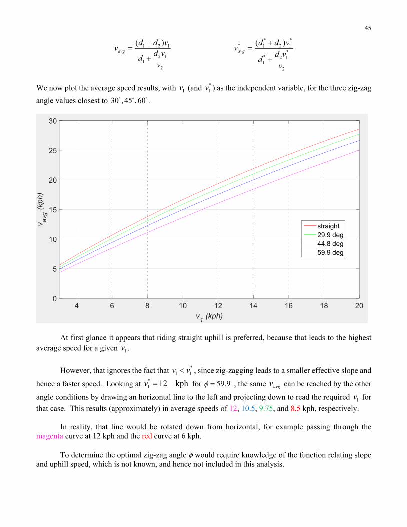
We now plot the average speed results, with 1v (and *1v ) as the independent variable, for the three zig-zag
angle values closest to 30 ,45 ,60 .
At first glance it appears that riding straight uphill is preferred, because that leads to the highest average speed for a given 1v .
However, that ignores the fact that *1 1v v , since zig-zagging leads to a smaller effective slope and
hence a faster speed. Looking at *1 12 kphv for 59.9 , the same avgv can be reached by the other
angle conditions by drawing an horizontal line to the left and projecting down to read the required 1v for
that case. This results (approximately) in average speeds of 12, 10.5, 9.75, and 8.5 kph, respectively.
In reality, that line would be rotated down from horizontal, for example passing through the magenta curve at 12 kph and the red curve at 6 kph.
To determine the optimal zig-zag angle would require knowledge of the function relating slope
and uphill speed, which is not known, and hence not included in this analysis.
4 6 8 10 12 14 16 18 20
v1 (kph)
0
5
10
15
20
25
30
v avg (
kph)
straight29.9 deg44.8 deg59.9 deg
46
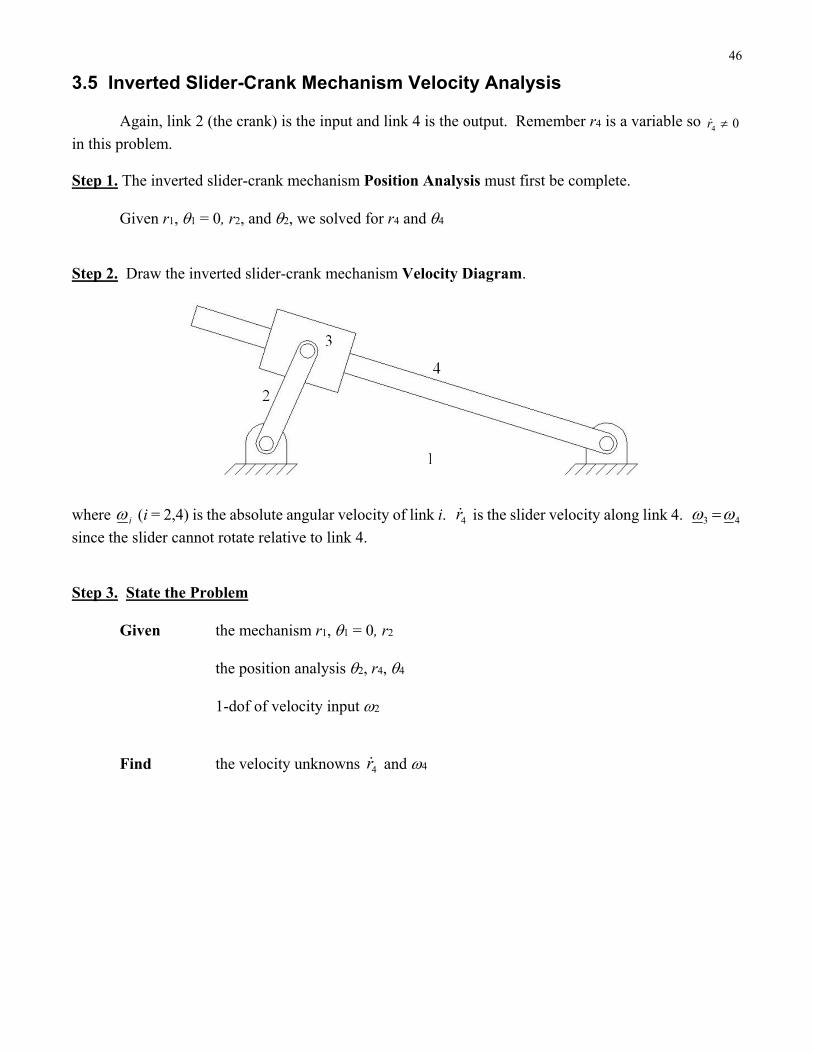
3.5 Inverted Slider-Crank Mechanism Velocity Analysis Again, link 2 (the crank) is the input and link 4 is the output. Remember r4 is a variable so
4 0r
in this problem. Step 1. The inverted slider-crank mechanism Position Analysis must first be complete. Given r1, 1 = 0, r2, and 2, we solved for r4 and 4 Step 2. Draw the inverted slider-crank mechanism Velocity Diagram.
where i (i = 2,4) is the absolute angular velocity of link i. 4r is the slider velocity along link 4. 3 4
since the slider cannot rotate relative to link 4. Step 3. State the Problem Given the mechanism r1, 1 = 0, r2
the position analysis 2, r4, 4
1-dof of velocity input 2
Find the velocity unknowns 4r and 4
47
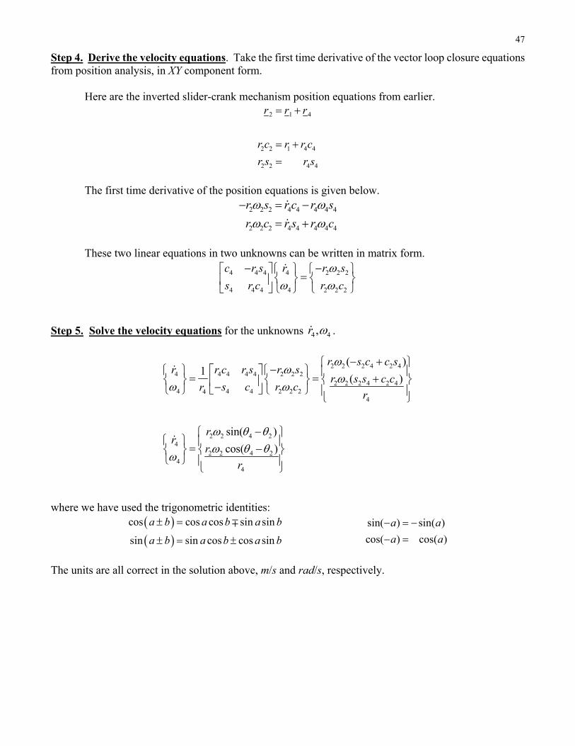
Step 4. Derive the velocity equations. Take the first time derivative of the vector loop closure equations from position analysis, in XY component form.
Here are the inverted slider-crank mechanism position equations from earlier.
2 1 4
2 2 1 4 4
2 2 4 4
r r r
r c r r c
r s r s
The first time derivative of the position equations is given below.
2 2 2 4 4 4 4 4
2 2 2 4 4 4 4 4
r s r c r s
r c r s r c
These two linear equations in two unknowns can be written in matrix form.
4 4 4 4 2 2 2
4 4 4 4 2 2 2
c r s r r s
s r c r c
Step 5. Solve the velocity equations for the unknowns 4 4,r .
2 2 2 4 2 44 4 4 4 4 2 2 2
2 2 2 4 2 44 4 4 2 2 24
4
2 2 4 24
2 2 4 24
4
( )1
( )
sin( )
cos( )
r s c c sr r c r s r s
r s s c cs c r cr
r
rr
r
r
where we have used the trigonometric identities:
cos cos cos sin sin
sin sin cos cos sin
a b a b a b
a b a b a b
sin( ) sin( )
cos( ) cos( )
a a
a a
The units are all correct in the solution above, m/s and rad/s, respectively.
48
Inverted slider-crank mechanism singularity condition When does the solution fail? This is an inverted slider-crank mechanism singularity, when the determinant of the coefficient matrix goes to zero. The result is dividing by zero, resulting in infinite
4 4,r .
4 4 4
4 4 4
c r sA
s r c
2 2 2 2
4 4 4 4 4 4 4 4( ) ( ) 0A r c r s r c s r
Physically, assuming
1 2r r as in the full rotation condition from the inverted slider-crank mechanism
position analysis, this is impossible, i.e. r4 never goes to zero.
This matrix determinant 4A r was used in the solution of the previous page.
Inverted slider-crank mechanism velocity example – Term Example 3 continued
Given
1
2
4
1
0.20
0.10
0.32
0
r
r
L
(m)
2
4
4
70
150.5
0.191r
(deg and m)
Snapshot Analysis Given this mechanism position analysis plus 2 25 rad/s, calculate 4 4,r for this snapshot.
4
4
0.870 0.094 2.349
0.493 0.166 0.855
r
4
4
2.47
2.18
r
(m/s and rad/s)
Both are positive, so the slider link 3 is currently traveling up link 4 and link 4 is currently rotating in the ccw direction, which makes sense from the physical problem.
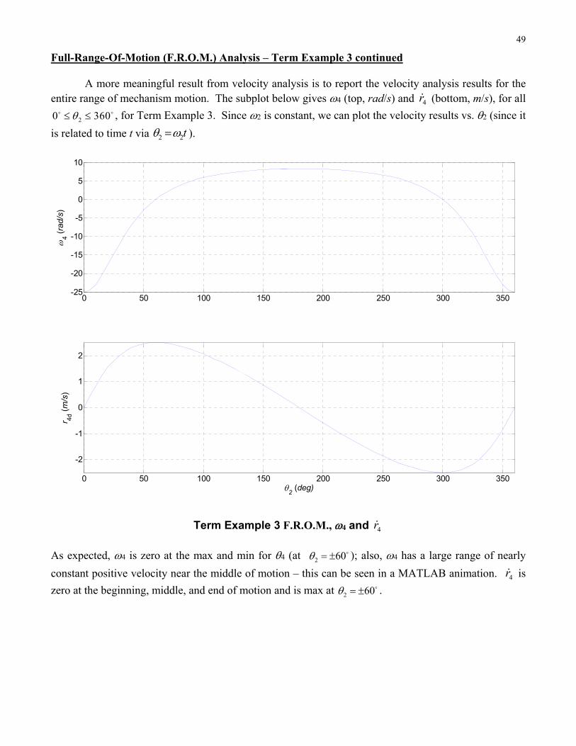
49
Full-Range-Of-Motion (F.R.O.M.) Analysis – Term Example 3 continued A more meaningful result from velocity analysis is to report the velocity analysis results for the entire range of mechanism motion. The subplot below gives 4 (top, rad/s) and 4r (bottom, m/s), for all
20 360 , for Term Example 3. Since 2 is constant, we can plot the velocity results vs. 2 (since it
is related to time t via 2 2t ).
Term Example 3 F.R.O.M., 4 and 4r
As expected, 4 is zero at the max and min for 4 (at 2 60 ); also, 4 has a large range of nearly
constant positive velocity near the middle of motion – this can be seen in a MATLAB animation. 4r is
zero at the beginning, middle, and end of motion and is max at 2 60 .
0 50 100 150 200 250 300 350-25
-20
-15
-10
-5
0
5
10
4 (
rad/
s)
0 50 100 150 200 250 300 350
-2
-1
0
1
2
2 (deg)
r 4d (
m/s
)

50
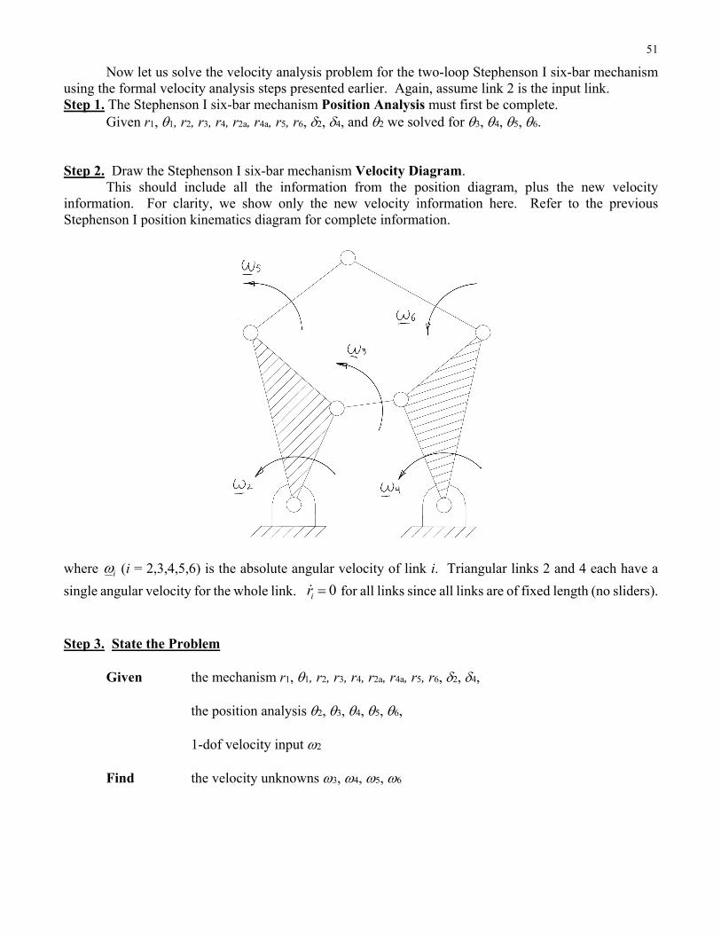
3.6 Multi-Loop Mechanism Velocity Analysis Thus far we have presented velocity analysis for the single-loop four-bar, slider-crank, and inverted slider-crank mechanisms. The velocity analysis for mechanisms of more than one loop is handled using the same general procedures developed for the single loop mechanisms. This section presents velocity analysis for the two-loop Stephenson I six-bar mechanism shown below as an example multi-loop mechanism. It follows the position analysis for the same mechanism presented earlier.
Stephenson I 6-Bar Mechanism The bottom loop of the Stephenson I six-bar mechanism is identical to the standard four-bar mechanism model and so the velocity analysis solution is identical to the four-bar presented earlier. With the complete velocity analysis of the bottom loop thus solved, the solution for the top loop is essentially another four-bar velocity solution. As in all velocity analysis, the velocity solution for multi-loop mechanisms is a linear analysis yielding a unique solution (assuming the given mechanism position is not singular) for each position solution branch considered. The position analysis must be complete prior to the velocity solution.
51
Now let us solve the velocity analysis problem for the two-loop Stephenson I six-bar mechanism using the formal velocity analysis steps presented earlier. Again, assume link 2 is the input link. Step 1. The Stephenson I six-bar mechanism Position Analysis must first be complete. Given r1, 1, r2, r3, r4, r2a, r4a, r5, r6, 2, 4, and 2 we solved for 3, 4, 5, 6. Step 2. Draw the Stephenson I six-bar mechanism Velocity Diagram.
This should include all the information from the position diagram, plus the new velocity information. For clarity, we show only the new velocity information here. Refer to the previous Stephenson I position kinematics diagram for complete information.
where i (i = 2,3,4,5,6) is the absolute angular velocity of link i. Triangular links 2 and 4 each have a
single angular velocity for the whole link. 0ir for all links since all links are of fixed length (no sliders).
Step 3. State the Problem Given the mechanism r1, 1, r2, r3, r4, r2a, r4a, r5, r6, 2, 4, the position analysis 2, 3, 4, 5, 6,
1-dof velocity input 2
Find the velocity unknowns 3, 4, 5, 6
52
Step 4. Derive the velocity equations. Take the first time derivative of each of the two vector loop closure equations from position analysis, in XY component form. Here are the Stephenson I six-bar mechanism position equations. Vector equations
2 3 1 4
2 5 1 4 6a a
r r r r
r r r r r
XY scalar equations
2 2 3 3 1 1 4 4
2 2 3 3 1 1 4 4
r c r c rc r c
r s r s rs r s
2 2 5 5 1 1 4 4 6 6
2 2 5 5 1 1 4 4 6 6
a a a a
a a a a
r c r c rc r c r c
r s r s r s r s r s
where 2 2 2
4 4 4
a
a
The first time derivatives of the Loop I position equations are identical to those for the standard four-bar mechanism.
2 2 2 3 3 3 4 4 4
2 2 2 3 3 3 4 4 4
r s r s r s
r c r c r c
These equations can be written in matrix form.
3 3 4 4 3 2 2 2
3 3 4 4 4 2 2 2
r s r s r s
r c r c r c
The first time derivative of the Loop II position equations is
2 2 2 5 5 5 4 4 4 6 6 6
2 2 2 5 5 5 4 4 4 6 6 6
a a a a a a
a a a a a a
r s r s r s r s
r c r c r c r c
These equations can be written in matrix form.
5 5 6 6 5 2 2 2 4 4 4
5 5 6 6 6 2 2 2 4 4 4
a a a a
a a a a
r s r s r s r s
r c r c r c r c
where we have used 2 2
4 4
a
a
since 2 and 4 are constant angles.

53
Step 5. Solve the velocity equations for the unknowns 3, 4, 5, 6. The two mechanism loops decouple so we find 3 and 4 from Loop I first and then use 4 to find 5 and 6 from Loop II. The solutions are given below. Loop I (identical to the standard four-bar mechanism)
1
3 3 4 43 2 2 2
3 3 4 44 2 2 2
r s r s r s
r c r c r c
Loop II (similar to the standard four-bar mechanism)
1
5 5 5 6 6 2 2 2 4 4 4
6 5 5 6 6 2 2 2 4 4 4
a a a a
a a a a
r s r s r s r s
r c r c r c r c
Remember, Gaussian elimination is more efficient and robust than the matrix inverse. Also, these equations may be solved algebraically instead of using matrix methods to yield the same answers. Stephenson I six-bar mechanism singularity condition The velocity solution fails when the determinant of either coefficient matrix above goes to zero. The result is dividing by zero, resulting in infinite angular velocities for the associated loop. For the first loop, the singularity condition is identical to the singularity condition of the standard four-bar mechanism, i.e. when links 3 and 4 either line up or fold upon each other, causing a link 2 joint limit. For the second loop, the singularity condition is similar, occurring when links 5 and 6 either line up or fold upon each other. These conditions also cause angle limit problems for the position analysis, so the velocity singularities are known problems.
54
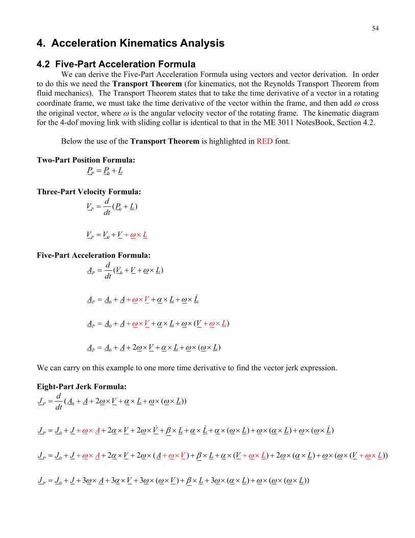
4. Acceleration Kinematics Analysis 4.2 Five-Part Acceleration Formula We can derive the Five-Part Acceleration Formula using vectors and vector derivation. In order to do this we need the Transport Theorem (for kinematics, not the Reynolds Transport Theorem from fluid mechanics). The Transport Theorem states that to take the time derivative of a vector in a rotating coordinate frame, we must take the time derivative of the vector within the frame, and then add cross the original vector, where is the angular velocity vector of the rotating frame. The kinematic diagram for the 4-dof moving link with sliding collar is identical to that in the ME 3011 NotesBook, Section 4.2. Below the use of the Transport Theorem is highlighted in RED font. Two-Part Position Formula:
0PP P L
Three-Part Velocity Formula:
0
0
( )P
P
dV P L
dt
V LV V
Five-Part Acceleration Formula:
0
0
0
0
( )
( )
2 ( )
P
P
P
P
dA V V L
dt
A A A L L
A A A L V
A
V
V L
A A V L L
We can carry on this example to one more time derivative to find the vector jerk expression. Eight-Part Jerk Formula:
0
0
0
0
( 2 ( ))
2 2 ( ) ( ) ( )
2 2 ( ) ( ) 2 ( ) ( ( ))
3 3 3 ( ) 3 ( ) ( ( ))
P
P
P
P
dJ A A V L L
dt
J J J V V L L L L L
J J J V
A
A L V L V
J J J
A V L L
A V V L L L
55
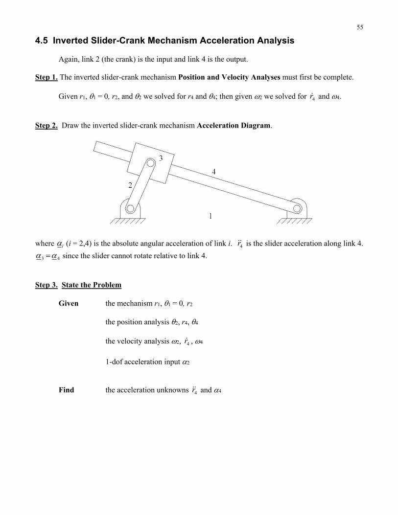
4.5 Inverted Slider-Crank Mechanism Acceleration Analysis Again, link 2 (the crank) is the input and link 4 is the output. Step 1. The inverted slider-crank mechanism Position and Velocity Analyses must first be complete. Given r1, 1 = 0, r2, and 2 we solved for r4 and 4; then given 2 we solved for 4r and 4.
Step 2. Draw the inverted slider-crank mechanism Acceleration Diagram.
where i (i = 2,4) is the absolute angular acceleration of link i. 4r is the slider acceleration along link 4.
3 4 since the slider cannot rotate relative to link 4.
Step 3. State the Problem Given the mechanism r1, 1 = 0, r2
the position analysis 2, r4, 4 the velocity analysis 2, 4r , 4
1-dof acceleration input 2
Find the acceleration unknowns 4r and 4
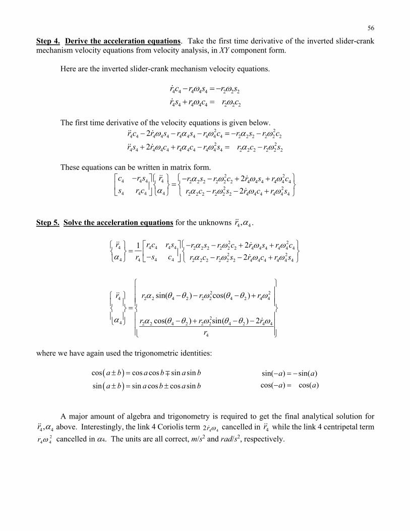
56
Step 4. Derive the acceleration equations. Take the first time derivative of the inverted slider-crank mechanism velocity equations from velocity analysis, in XY component form.
Here are the inverted slider-crank mechanism velocity equations.
4 4 4 4 4 2 2 2
4 4 4 4 4 2 2 2
r c r s r s
r s r c r c
The first time derivative of the velocity equations is given below.
2 24 4 4 4 4 4 4 4 4 4 4 2 2 2 2 2 2
2 24 4 4 4 4 4 4 4 4 4 4 2 2 2 2 2 2
2
2
r c r s r s r c r s r c
r s r c r c r s r c r s
These equations can be written in matrix form.
2 24 4 4 4 2 2 2 2 2 2 4 4 4 4 4 4
2 24 4 4 4 2 2 2 2 2 2 4 4 4 4 4 4
2
2
c r s r r s r c r s r c
s r c r c r s r c r s
Step 5. Solve the acceleration equations for the unknowns 4 4,r .
2 2
4 4 4 4 4 2 2 2 2 2 2 4 4 4 4 4 42 2
4 4 44 2 2 2 2 2 2 4 4 4 4 4 4
2 24 2 2 4 2 2 2 4 2 4 4
24 2 2 4 2 2 2 4 2 4 4
4
21
2
sin( ) cos( )
cos( ) sin( ) 2
r r c r s r s r c r s r c
s cr r c r s r c r s
r r r r
r r r
r
where we have again used the trigonometric identities:
cos cos cos sin sin
sin sin cos cos sin
a b a b a b
a b a b a b
sin( ) sin( )
cos( ) cos( )
a a
a a
A major amount of algebra and trigonometry is required to get the final analytical solution for
4 4,r above. Interestingly, the link 4 Coriolis term 4 42r cancelled in 4r while the link 4 centripetal term
24 4r cancelled in 4. The units are all correct, m/s2 and rad/s2, respectively.
57
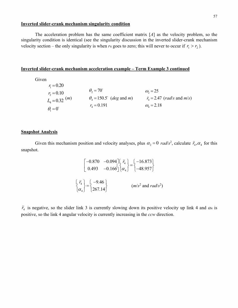
Inverted slider-crank mechanism singularity condition The acceleration problem has the same coefficient matrix [A] as the velocity problem, so the singularity condition is identical (see the singularity discussion in the inverted slider-crank mechanism velocity section – the only singularity is when r4 goes to zero; this will never to occur if 1 2r r ).
Inverted slider-crank mechanism acceleration example – Term Example 3 continued
Given
1
2
4
1
0.20
0.10
0.32
0
r
r
L
(m)
2
4
4
70
150.5
0.191r
(deg and m) 2
4
4
25
2.47
2.18
r
(rad/s and m/s)
Snapshot Analysis Given this mechanism position and velocity analyses, plus 2 0 rad/s2, calculate 4 4,r for this
snapshot.
4
4
0.870 0.094 16.873
0.493 0.166 48.957
r
4
4
9.46
267.14
r
(m/s2 and rad/s2)
4r is negative, so the slider link 3 is currently slowing down its positive velocity up link 4 and 4 is
positive, so the link 4 angular velocity is currently increasing in the ccw direction.
58
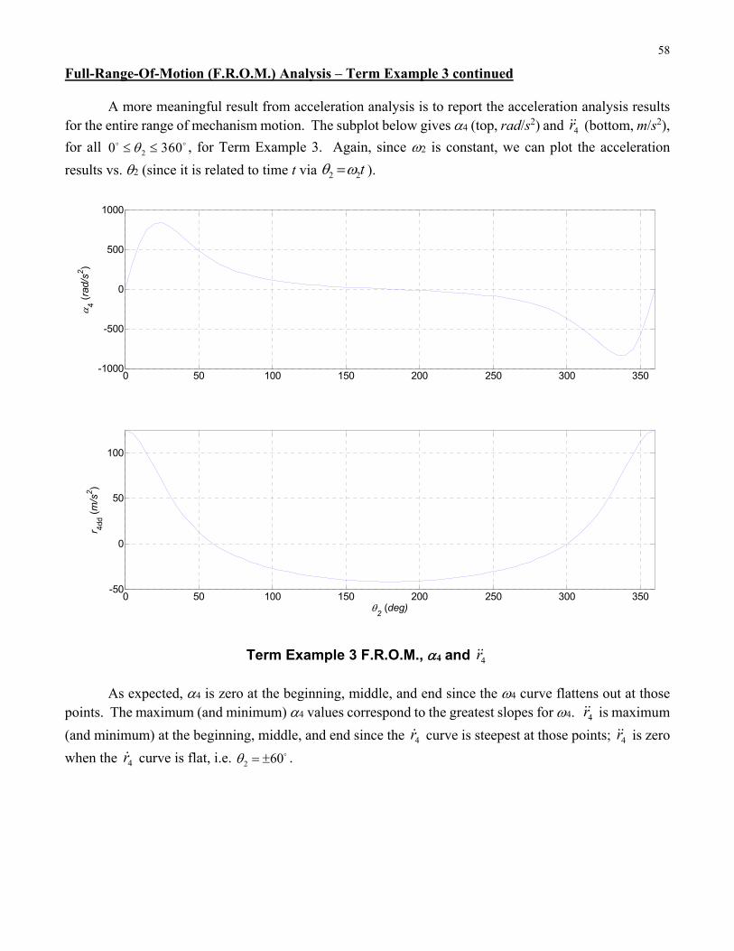
Full-Range-Of-Motion (F.R.O.M.) Analysis – Term Example 3 continued A more meaningful result from acceleration analysis is to report the acceleration analysis results for the entire range of mechanism motion. The subplot below gives 4 (top, rad/s2) and 4r (bottom, m/s2),
for all 20 360 , for Term Example 3. Again, since 2 is constant, we can plot the acceleration
results vs. 2 (since it is related to time t via 2 2t ).
Term Example 3 F.R.O.M., 4 and 4r
As expected, 4 is zero at the beginning, middle, and end since the 4 curve flattens out at those
points. The maximum (and minimum) 4 values correspond to the greatest slopes for 4. 4r is maximum
(and minimum) at the beginning, middle, and end since the 4r curve is steepest at those points; 4r is zero
when the 4r curve is flat, i.e. 2 60 .
0 50 100 150 200 250 300 350-1000
-500
0
500
1000
4 (
rad/
s2 )
0 50 100 150 200 250 300 350-50
0
50
100
2 (deg)
r 4dd (
m/s
2 )
59
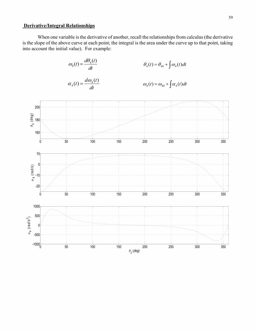
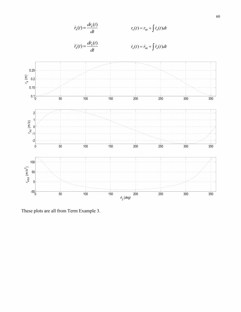
Derivative/Integral Relationships When one variable is the derivative of another, recall the relationships from calculus (the derivative is the slope of the above curve at each point; the integral is the area under the curve up to that point, taking into account the initial value). For example:
44
( )( )
d tt
dt
4 40 4( ) ( )t t dt
44
( )( )
d tt
dt
4 40 4( ) ( )t t dt
0 50 100 150 200 250 300 350
160
180
200
4 (
deg)
0 50 100 150 200 250 300 350
-20
-10
0
10
4
(ra
d/s )
0 50 100 150 200 250 300 350-1000
-500
0
500
1000
2 (deg)
4 (
rad/
s2 )
60
44
( )( )
dr tr t
dt 4 40 4( ) ( )r t r r t dt
44
( )( )
dr tr t
dt 4 40 4( ) ( )r t r r t dt
These plots are all from Term Example 3.
0 50 100 150 200 250 300 3500.1
0.15
0.2
0.25
r 4 (
m)
0 50 100 150 200 250 300 350
-2
-1
0
1
2
r 4d (
m/s
)
0 50 100 150 200 250 300 350-50
0
50
100
2 (deg)
r 4d
d (
m/s
2)
61
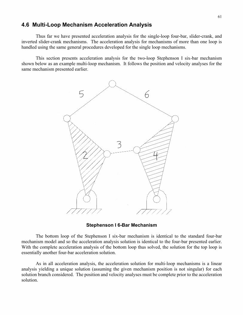
4.6 Multi-Loop Mechanism Acceleration Analysis Thus far we have presented acceleration analysis for the single-loop four-bar, slider-crank, and inverted slider-crank mechanisms. The acceleration analysis for mechanisms of more than one loop is handled using the same general procedures developed for the single loop mechanisms. This section presents acceleration analysis for the two-loop Stephenson I six-bar mechanism shown below as an example multi-loop mechanism. It follows the position and velocity analyses for the same mechanism presented earlier.
Stephenson I 6-Bar Mechanism The bottom loop of the Stephenson I six-bar mechanism is identical to the standard four-bar mechanism model and so the acceleration analysis solution is identical to the four-bar presented earlier. With the complete acceleration analysis of the bottom loop thus solved, the solution for the top loop is essentially another four-bar acceleration solution. As in all acceleration analysis, the acceleration solution for multi-loop mechanisms is a linear analysis yielding a unique solution (assuming the given mechanism position is not singular) for each solution branch considered. The position and velocity analyses must be complete prior to the acceleration solution.

62
Now let us solve the acceleration analysis problem for the two-loop Stephenson I six-bar mechanism using the formal acceleration analysis steps presented earlier. Again, assume link 2 is the input link. Step 1. The Stephenson I six-bar mechanism Position and Velocity Analyses must first be complete. Given r1, 1, r2, r3, r4, r2a, r4a, r5, r6, 2, 4, 2, and 2, we solved for 3, 4, 5, 6, 3, 4, 5, 6. Step 2. Draw the Stephenson I six-bar mechanism Acceleration Diagram.
This should include all the information from the position and velocity diagrams, plus the new acceleration information. For clarity, we show only the new acceleration information here. Refer to the previous Stephenson I position and velocity kinematics diagrams for complete information.
where i (i = 2,3,4,5,6) is the absolute angular acceleration of link i. Triangular links 2 and 4 each have
a single angular acceleration for the whole link. 0ir for all links since all links are of fixed length (no
sliders). Step 3. State the Problem Given the mechanism r1, 1, r2, r3, r4, r2a, r4a, r5, r6, 2, 4, the position analysis 2, 3, 4, 5, 6,
the velocity analysis 2, 3, 4, 5, 6, 1-dof acceleration input 2
Find the acceleration unknowns 3, 4, 5, 6
63
Step 4. Derive the acceleration equations. Take the first time derivative of both sides of each of the four scalar XY velocity equations. The Stephenson I six-bar mechanism velocity equations are given below. XY scalar velocity equations
2 2 2 3 3 3 4 4 4
2 2 2 3 3 3 4 4 4
r s r s r s
r c r c r c
2 2 2 5 5 5 4 4 4 6 6 6
2 2 2 5 5 5 4 4 4 6 6 6
a a a a a a
a a a a a a
r s r s r s r s
r c r c r c r c
where 2 2 2
4 4 4
a
a
The first time derivative of the Loop I velocity equations is identical to that for the standard four-bar mechanism.
2 2 22 2 2 2 2 2 3 3 3 3 3 3 4 4 4 4 4 4
2 2 22 2 2 2 2 2 3 3 3 3 3 3 4 4 4 4 4 4
r s r c r s r c r s r c
r c r s r c r s r c r s
These equations can be written in matrix form.
2 2 23 3 4 4 3 2 2 2 2 2 2 3 3 3 4 4 4
2 2 23 3 4 4 4 2 2 2 2 2 2 3 3 3 4 4 4
r s r s r s r c r c r c
r c r c r c r s r s r s
The first time derivatives of the Loop II velocity equations are:
2 2 2 22 2 2 2 2 2 5 5 5 5 5 5 4 4 4 4 4 4 6 6 6 6 6 6
2 2 2 22 2 2 2 2 2 5 5 5 5 5 5 4 4 4 4 4 4 6 6 6 6 6 6
a a a a a a a a a a a a
a a a a a a a a a a a a
r s r c r s r c r s r c r s r c
r c r s r c r s r c r s r c r s
These equations can be written in matrix form.
2 2 2 25 5 6 6 5 2 2 2 2 2 2 5 5 5 4 4 4 4 4 4 6 6 6
2 2 2 25 5 6 6 6 2 2 2 2 2 2 5 5 5 4 4 4 4 4 4 6 6 6
a a a a a a a a
a a a a a a a a
r s r s r s r c r c r s r c r c
r c r c r c r s r s r c r s r s
where we have used 2 2
4 4
a
a
and
2 2
4 4
a
a
since 2 and 4 are constant angles.

64
Step 5. Solve the acceleration equations for the unknowns 3, 4, 5, 6. The two loops decouple so we find 3 and 4 from Loop I first and then use 4 to find 5 and 6 from Loop II. The solutions are given below. Loop I (identical to the standard four-bar mechanism)
1 2 2 23 3 4 43 2 2 2 2 2 2 3 3 3 4 4 4
2 2 23 3 4 44 2 2 2 2 2 2 3 3 3 4 4 4
r s r s r s r c r c r c
r c r c r c r s r s r s
Loop II (similar to the standard four-bar mechanism)
1 2 2 2 25 5 5 6 6 2 2 2 2 2 2 5 5 5 4 4 4 4 4 4 6 6 6
2 2 2 26 5 5 6 6 2 2 2 2 2 2 5 5 5 4 4 4 4 4 4 6 6 6
a a a a a a a a
a a a a a a a a
r s r s r s r c r c r s r c r c
r c r c r c r s r s r c r s r s
Remember, Gaussian elimination is more efficient and robust than the matrix inverse. Also, these equations may easily be solved algebraically instead of using matrix methods. Stephenson I six-bar mechanism singularity condition The acceleration solution fails when the determinant of either coefficient matrix above goes to zero. The result is dividing by zero, resulting in infinite angular accelerations for the associated loop. Note the two coefficients matrices in the acceleration solutions are identical to those for the velocity solutions. Therefore, the acceleration singularity conditions are identical to the velocity singularity conditions. For the first loop, the singularity condition is identical to the singularity condition of the standard four-bar mechanism, i.e. when links 3 and 4 either line up or fold upon each other, causing a link 2 joint limit. For the second loop, the singularity condition is similar, occurring when 5 and 6 either line up or fold upon each other. These conditions also cause problems for the velocity and position analyses, so the acceleration singularities are known problems.
65
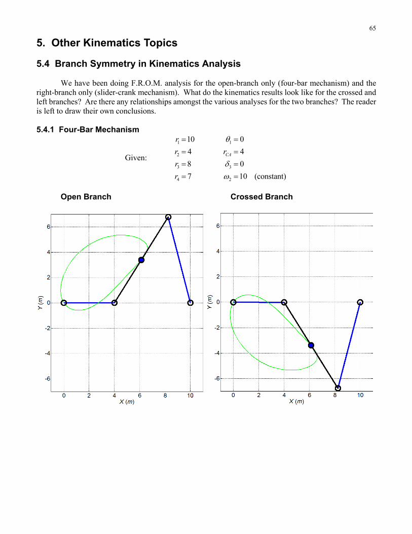
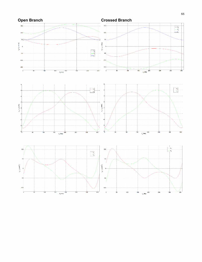
5. Other Kinematics Topics 5.4 Branch Symmetry in Kinematics Analysis We have been doing F.R.O.M. analysis for the open-branch only (four-bar mechanism) and the right-branch only (slider-crank mechanism). What do the kinematics results look like for the crossed and left branches? Are there any relationships amongst the various analyses for the two branches? The reader is left to draw their own conclusions. 5.4.1 Four-Bar Mechanism
Given:
1
2
3
4
10
4
8
7
r
r
r
r
1
3
2
0
4
0
10 (constant)
CAr
Open Branch Crossed Branch
66
Open Branch Crossed Branch
67
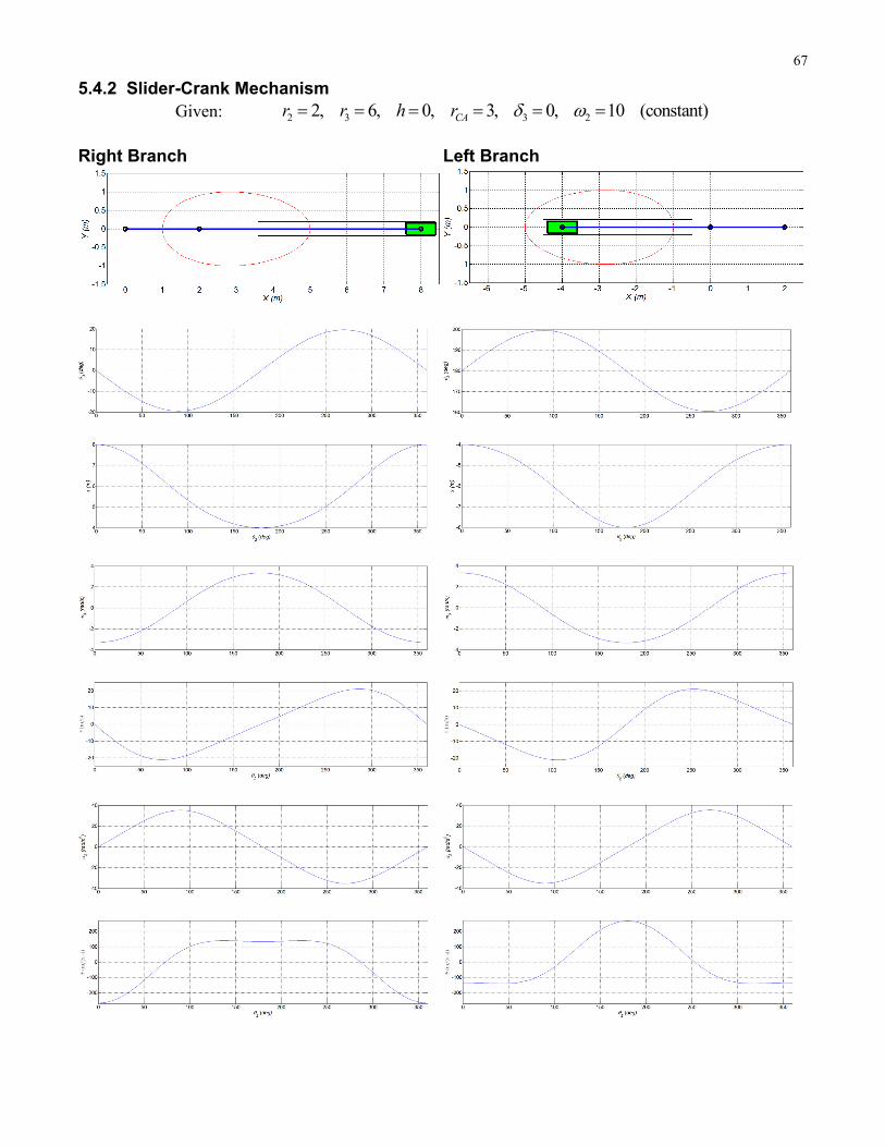
5.4.2 Slider-Crank Mechanism Given: 2 3 3 22, 6, 0, 3, 0, 10 (constant)CAr r h r
Right Branch Left Branch

68
We see a great deal of symmetry for both four-bar and slider crank mechanism kinematic analyses.
The coupler point curves and all plots have either horizontal midpoint 2 180 or vertical zero point flip-
symmetry (some have both). However, for the x and x slider-crank mechanism results, this symmetry is not immediately
evident. This special symmetry is revealed when first cutting the plots at 2 180 , and then performing
the horizontal and/or vertical flipping.
69
6. Inverse Dynamics Analysis 6.1 Dynamics Introduction D’Alembert’s Principle We can convert dynamics problems into statics problems by the inclusion of a vector inertial force
0 GF m A and a vector inertial moment 0 GM I . Centrifugal force 2mr , directed away from
the center of rotation, is an example of an inertial force vector. It’s not really a force but a felt effect of an inertia in acceleration. Using D’Alembert’s principle, the right-hand side of the translational and rotational dynamics equations is subtracted to the other side of the equation. Then the forces and moments balance to zero as in statics, when the inertial forces are included in the FBD.
We won’t use this method, but it is mentioned for completeness. We would instead to prefer to consider statics problems as a subset of dynamics problems, with zero accelerations.
0
0
G
O
R mA
R F
0
0
G
O
T r R I
T r R M
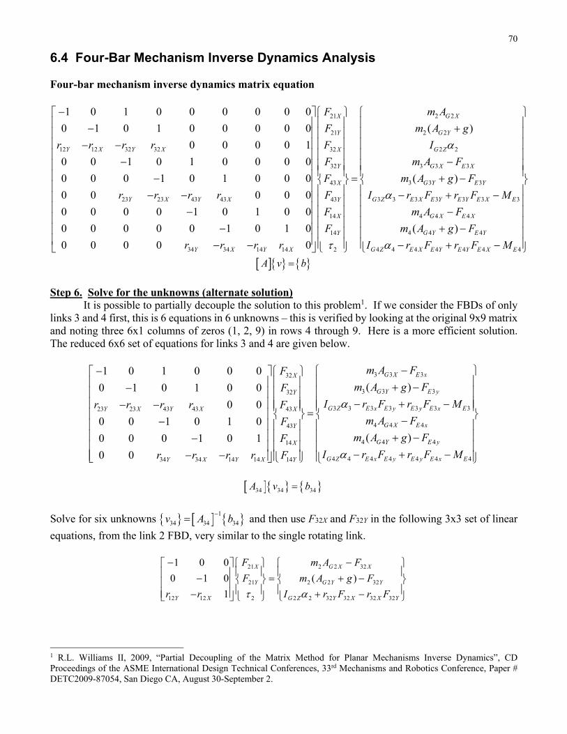
70
6.4 Four-Bar Mechanism Inverse Dynamics Analysis Four-bar mechanism inverse dynamics matrix equation
21
21
12 12 32 32 32
32
43
23 23 43 43 43
14
14
34 34 14 14 2
1 0 1 0 0 0 0 0 0
0 1 0 1 0 0 0 0 0
0 0 0 0 1
0 0 1 0 1 0 0 0 0
0 0 0 1 0 1 0 0 0
0 0 0 0 0
0 0 0 0 1 0 1 0 0
0 0 0 0 0 1 0 1 0
0 0 0 0 0
X
Y
Y X Y X X
Y
X
Y X Y X Y
X
Y
Y X Y X
F
F
r r r r F
F
F
r r r r F
F
F
r r r r
2 2
2 2
2 2
3 3 3
3 3 3
3 3 3 3 3 3 3
4 4 4
4 4 4
4 4 4 4 4 4 4
( )
( )
( )
G X
G Y
G Z
G X E X
G Y E Y
G Z E X E Y E Y E X E
G X E X
G Y E Y
G Z E X E Y E Y E X E
m A
m A g
I
m A F
m A g F
I r F r F M
m A F
m A g F
I r F r F M
A v b
Step 6. Solve for the unknowns (alternate solution) It is possible to partially decouple the solution to this problem1. If we consider the FBDs of only links 3 and 4 first, this is 6 equations in 6 unknowns – this is verified by looking at the original 9x9 matrix and noting three 6x1 columns of zeros (1, 2, 9) in rows 4 through 9. Here is a more efficient solution. The reduced 6x6 set of equations for links 3 and 4 are given below.
3 3 332
3 3 332
3 3 3 3 3 3 323 23 43 43 43
4 4 443
14
34 34 14 14 14
1 0 1 0 0 0
( )0 1 0 1 0 0
0 0
0 0 1 0 1 0
0 0 0 1 0 1
0 0
G X E xX
G Y E yY
G Z E x E y E y E x EY X Y X X
G X E xY
X
Y X Y X Y
m A FF
m A g FF
I r F r F Mr r r r F
m A FF
F
r r r r F
4 4 4
4 4 4 4 4 4 4
( )G Y E y
G Z E x E y E y E x E
m A g F
I r F r F M
34 34 34A v b
Solve for six unknowns 1
34 34 34v A b and then use F32X and F32Y in the following 3x3 set of linear
equations, from the link 2 FBD, very similar to the single rotating link.
21 2 2 32
21 2 2 32
12 12 2 2 2 32 32 32 32
1 0 0
0 1 0 ( )
1
X G X X
Y G Y Y
Y X G Z Y X X Y
F m A F
F m A g F
r r I r F r F
1 R.L. Williams II, 2009, “Partial Decoupling of the Matrix Method for Planar Mechanisms Inverse Dynamics”, CD Proceedings of the ASME International Design Technical Conferences, 33rd Mechanisms and Robotics Conference, Paper # DETC2009-87054, San Diego CA, August 30-September 2.
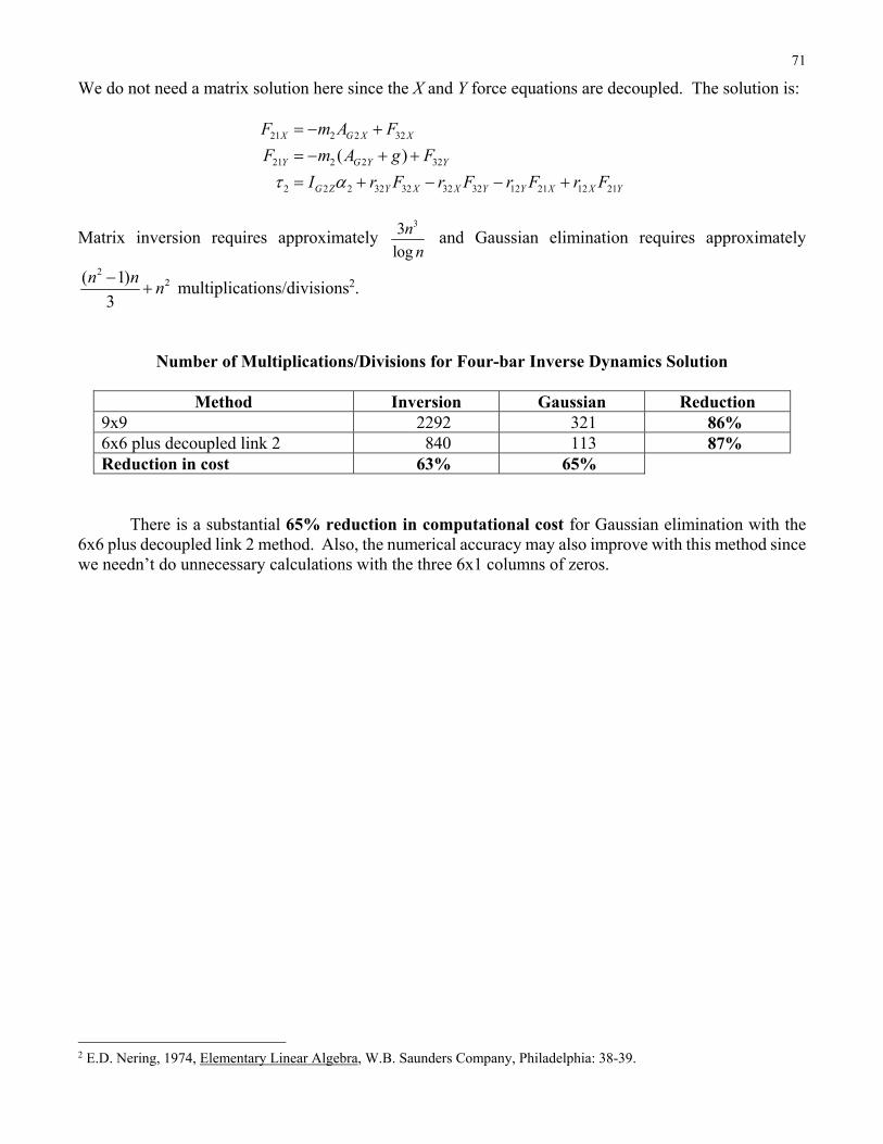
71
We do not need a matrix solution here since the X and Y force equations are decoupled. The solution is:
21 2 2 32
21 2 2 32
2 2 2 32 32 32 32 12 21 12 21
( )X G X X
Y G Y Y
G Z Y X X Y Y X X Y
F m A F
F m A g F
I r F r F r F r F
Matrix inversion requires approximately 33
log
n
n and Gaussian elimination requires approximately
22( 1)
3
n nn
multiplications/divisions2.
Number of Multiplications/Divisions for Four-bar Inverse Dynamics Solution
Method Inversion Gaussian Reduction 9x9 2292 321 86% 6x6 plus decoupled link 2 840 113 87% Reduction in cost 63% 65%
There is a substantial 65% reduction in computational cost for Gaussian elimination with the 6x6 plus decoupled link 2 method. Also, the numerical accuracy may also improve with this method since we needn’t do unnecessary calculations with the three 6x1 columns of zeros.
2 E.D. Nering, 1974, Elementary Linear Algebra, W.B. Saunders Company, Philadelphia: 38-39.
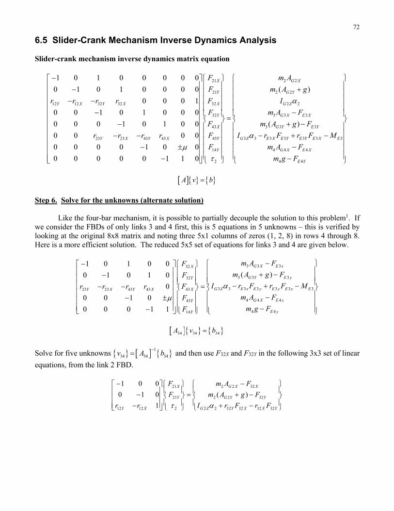
72
6.5 Slider-Crank Mechanism Inverse Dynamics Analysis Slider-crank mechanism inverse dynamics matrix equation
21 2 2
21 2 2
3212 12 32 32
32
43
4323 23 43 43
14
2
1 0 1 0 0 0 0 0
( )0 1 0 1 0 0 0 0
0 0 0 1
0 0 1 0 1 0 0 0
0 0 0 1 0 1 0 0
0 0 0 0
0 0 0 0 1 0 0
0 0 0 0 0 1 1 0
X G X
Y G Y
X GY X Y X
Y
X
YY X Y X
Y
F m A
F m A g
F Ir r r r
F
F
Fr r r r
F
2 2
3 3 3
3 3 3
3 3 3 3 3 3 3
4 4 4
4 4
( )
Z
G X E X
G Y E Y
G Z E X E Y E Y E X E
G X E X
E Y
m A F
m A g F
I r F r F M
m A F
m g F
A v b
Step 6. Solve for the unknowns (alternate solution) Like the four-bar mechanism, it is possible to partially decouple the solution to this problem1. If we consider the FBDs of only links 3 and 4 first, this is 5 equations in 5 unknowns – this is verified by looking at the original 8x8 matrix and noting three 5x1 columns of zeros (1, 2, 8) in rows 4 through 8. Here is a more efficient solution. The reduced 5x5 set of equations for links 3 and 4 are given below.
3 3 332
3 3 332
3 3 3 3 3 3 34323 23 43 43
4 4 443
4 414
1 0 1 0 0
( )0 1 0 1 0
0
0 0 1 0
0 0 0 1 1
G X E xX
G Y E yY
G Z E x E y E y E x EXY X Y X
G X E xY
E yY
m A FF
m A g FF
I r F r F MFr r r r
m A FF
m g FF
34 34 34A v b
Solve for five unknowns 1
34 34 34v A b and then use F32X and F32Y in the following 3x3 set of linear
equations, from the link 2 FBD.
21 2 2 32
21 2 2 32
12 12 2 2 2 32 32 32 32
1 0 0
0 1 0 ( )
1
X G X X
Y G Y Y
Y X G Z Y X X Y
F m A F
F m A g F
r r I r F r F
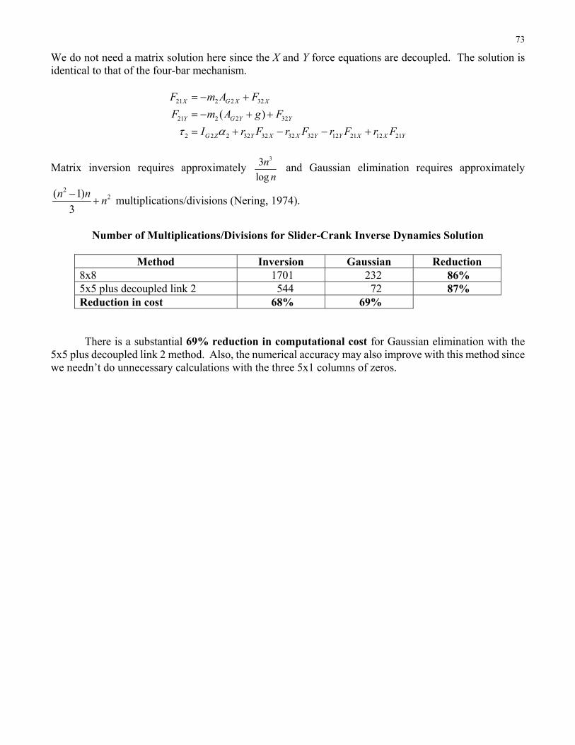
73
We do not need a matrix solution here since the X and Y force equations are decoupled. The solution is identical to that of the four-bar mechanism.
21 2 2 32
21 2 2 32
2 2 2 32 32 32 32 12 21 12 21
( )X G X X
Y G Y Y
G Z Y X X Y Y X X Y
F m A F
F m A g F
I r F r F r F r F
Matrix inversion requires approximately 33
log
n
n and Gaussian elimination requires approximately
22( 1)
3
n nn
multiplications/divisions (Nering, 1974).
Number of Multiplications/Divisions for Slider-Crank Inverse Dynamics Solution
Method Inversion Gaussian Reduction
8x8 1701 232 86% 5x5 plus decoupled link 2 544 72 87% Reduction in cost 68% 69%
There is a substantial 69% reduction in computational cost for Gaussian elimination with the 5x5 plus decoupled link 2 method. Also, the numerical accuracy may also improve with this method since we needn’t do unnecessary calculations with the three 5x1 columns of zeros.
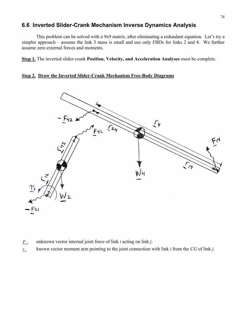
74
6.6 Inverted Slider-Crank Mechanism Inverse Dynamics Analysis This problem can be solved with a 9x9 matrix, after eliminating a redundant equation. Let’s try a simpler approach – assume the link 3 mass is small and use only FBDs for links 2 and 4. We further assume zero external forces and moments. Step 1. The inverted slider-crank Position, Velocity, and Acceleration Analyses must be complete. Step 2. Draw the Inverted Slider-Crank Mechanism Free-Body Diagrams
ijF unknown vector internal joint force of link i acting on link j.
ijr known vector moment arm pointing to the joint connection with link i from the CG of link j.
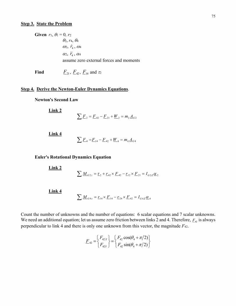
75
Step 3. State the Problem Given r1, 1 = 0, r2
2, r4, 4 2, 4r , 4
2, 4r , 4
assume zero external forces and moments
Find 21F , 42F , 14F and 2 Step 4. Derive the Newton-Euler Dynamics Equations.
Newton's Second Law Link 2
2 42 21 22 2 GF F F W m A
Link 4
4 14 42 44 4 GF F F W m A
Euler's Rotational Dynamics Equation Link 2
2 42 42 12 212 22G z G ZM r F r F I
Link 4
4 14 14 24 42 44G z G ZM r F r F I
Count the number of unknowns and the number of equations: 6 scalar equations and 7 scalar unknowns. We need an additional equation; let us assume zero friction between links 2 and 4. Therefore, 42F is always perpendicular to link 4 and there is only one unknown from this vector, the magnitude F42.
42 42 442
42 42 4
cos( 2)
sin( 2)X
Y
F FF
F F
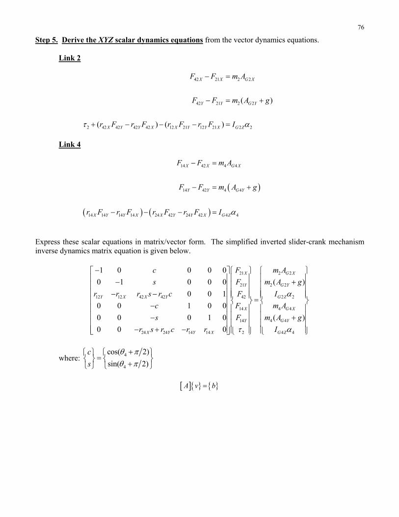
76
Step 5. Derive the XYZ scalar dynamics equations from the vector dynamics equations. Link 2
42 21 2 2
42 21 2 2
2 42 42 42 42 12 21 12 21 2 2
( )
( ) ( )
X X G X
Y Y G Y
X Y Y X X Y Y X G Z
F F m A
F F m A g
r F r F r F r F I
Link 4
14 42 4 4
14 42 4 4
14 14 14 14 24 42 24 42 4 4
X X G X
Y Y G Y
X Y Y X X Y Y X G Z
F F m A
F F m A g
r F r F r F r F I
Express these scalar equations in matrix/vector form. The simplified inverted slider-crank mechanism inverse dynamics matrix equation is given below.
2 221
2 221
2 212 12 42 42 42
4 414
4 414
4 424 24 14 14 2
1 0 0 0 0
( )0 1 0 0 0
0 0 1
0 0 1 0 0
( )0 0 0 1 0
0 0 0
G XX
G YY
G ZY X X Y
G XX
G YY
G ZX Y Y X
m Ac F
m A gs F
Ir r r s r c F
m Ac F
m A gs F
Ir s r c r r
where: 4
4
cos( 2)
sin( 2)
c
s
A v b
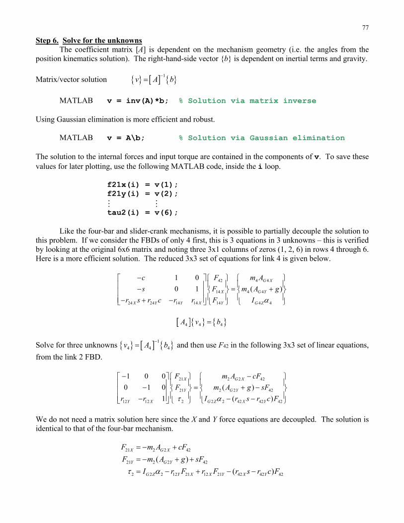
77
Step 6. Solve for the unknowns The coefficient matrix [A] is dependent on the mechanism geometry (i.e. the angles from the
position kinematics solution). The right-hand-side vector {b} is dependent on inertial terms and gravity.
Matrix/vector solution 1v A b
MATLAB v = inv(A)*b; % Solution via matrix inverse Using Gaussian elimination is more efficient and robust. MATLAB v = A\b; % Solution via Gaussian elimination The solution to the internal forces and input torque are contained in the components of v. To save these values for later plotting, use the following MATLAB code, inside the i loop. f21x(i) = v(1); f21y(i) = v(2); tau2(i) = v(6); Like the four-bar and slider-crank mechanisms, it is possible to partially decouple the solution to this problem. If we consider the FBDs of only 4 first, this is 3 equations in 3 unknowns – this is verified by looking at the original 6x6 matrix and noting three 3x1 columns of zeros (1, 2, 6) in rows 4 through 6. Here is a more efficient solution. The reduced 3x3 set of equations for link 4 is given below.
42 4 4
14 4 4
24 24 14 14 14 4 4
1 0
0 1 ( )G X
X G Y
X Y Y X Y G Z
c F m A
s F m A g
r s r c r r F I
4 4 4A v b
Solve for three unknowns 1
4 4 4v A b and then use F42 in the following 3x3 set of linear equations,
from the link 2 FBD.
21 2 2 42
21 2 2 42
12 12 2 2 2 42 42 42
1 0 0
0 1 0 ( )
1 ( )
X G X
Y G Y
Y X G Z X Y
F m A cF
F m A g sF
r r I r s r c F
We do not need a matrix solution here since the X and Y force equations are decoupled. The solution is identical to that of the four-bar mechanism.
21 2 2 42
21 2 2 42
2 2 2 12 21 12 21 42 42 42
( )
( )
X G X
Y G Y
G Z Y X X Y X Y
F m A cF
F m A g sF
I r F r F r s r c F
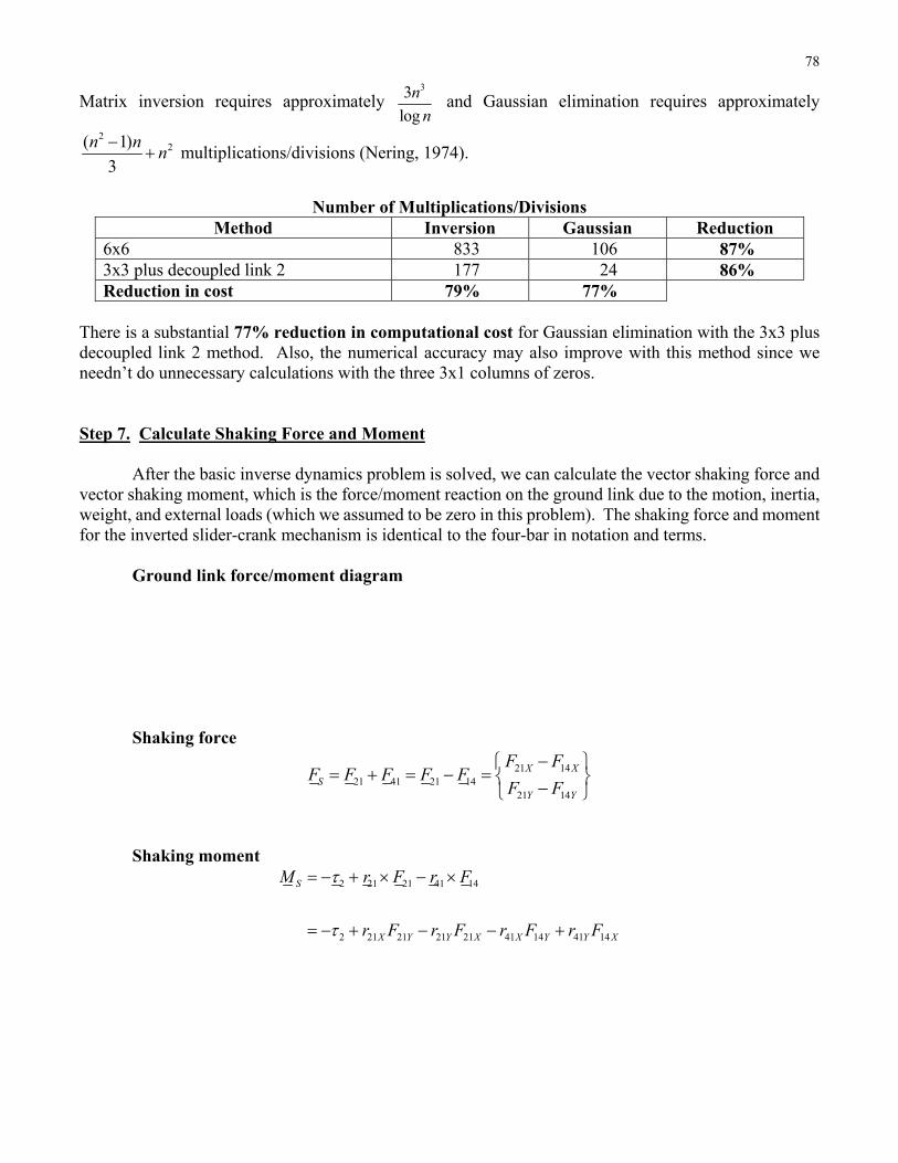
78
Matrix inversion requires approximately 33
log
n
n and Gaussian elimination requires approximately
22( 1)
3
n nn
multiplications/divisions (Nering, 1974).
Number of Multiplications/Divisions
Method Inversion Gaussian Reduction 6x6 833 106 87% 3x3 plus decoupled link 2 177 24 86% Reduction in cost 79% 77%
There is a substantial 77% reduction in computational cost for Gaussian elimination with the 3x3 plus decoupled link 2 method. Also, the numerical accuracy may also improve with this method since we needn’t do unnecessary calculations with the three 3x1 columns of zeros. Step 7. Calculate Shaking Force and Moment After the basic inverse dynamics problem is solved, we can calculate the vector shaking force and vector shaking moment, which is the force/moment reaction on the ground link due to the motion, inertia, weight, and external loads (which we assumed to be zero in this problem). The shaking force and moment for the inverted slider-crank mechanism is identical to the four-bar in notation and terms. Ground link force/moment diagram Shaking force
21 1421 41 21 14
21 14
X XS
Y Y
F FF F F F F
F F
Shaking moment
2 21 21 41 14
2 21 21 21 21 41 14 41 14
S
X Y Y X X Y Y X
M r F r F
r F r F r F r F
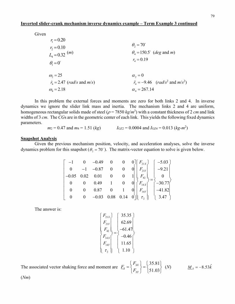
79
Inverted slider-crank mechanism inverse dynamics example – Term Example 3 continued
Given
1
2
4
1
0.20
0.10
0.32
0
r
r
L
(m)
2
4
4
70
150.5
0.19r
(deg and m)
2
4
4
25
2.47
2.18
r
(rad/s and m/s) 2
4
4
0
9.46
267.14
r
(rad/s2 and m/s2)
In this problem the external forces and moments are zero for both links 2 and 4. In inverse dynamics we ignore the slider link mass and inertia. The mechanism links 2 and 4 are uniform, homogeneous rectangular solids made of steel ( = 7850 kg/m3) with a constant thickness of 2 cm and link widths of 3 cm. The CGs are in the geometric center of each link. This yields the following fixed dynamics parameters.
m2 = 0.47 and m4 = 1.51 (kg) IGZ2 = 0.0004 and IGZ4 = 0.013 (kg-m2) Snapshot Analysis Given the previous mechanism position, velocity, and acceleration analyses, solve the inverse dynamics problem for this snapshot ( 2 70 ). The matrix-vector equation to solve is given below.
21
21
42
14
14
2
1 0 0.49 0 0 0 5.03
0 1 0.87 0 0 0 9.21
0.05 0.02 0.01 0 0 1 0
0 0 0.49 1 0 0 30.77
0 0 0.87 0 1 0 41.82
0 0 0.03 0.08 0.14 0 3.47
X
Y
X
Y
F
F
F
F
F
The answer is:
21
21
42
14
14
2
35.35
62.69
61.47
0.46
11.65
1.10
X
Y
X
Y
F
F
F
F
F
The associated vector shaking force and moment are 35.81
51.03SX
SSY
FF
F
(N) ˆ8.53SM k
(Nm)
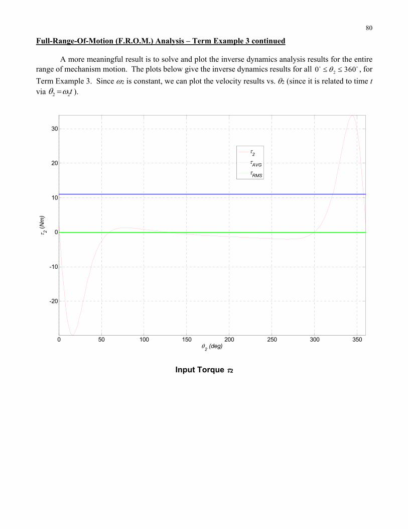
80
Full-Range-Of-Motion (F.R.O.M.) Analysis – Term Example 3 continued A more meaningful result is to solve and plot the inverse dynamics analysis results for the entire range of mechanism motion. The plots below give the inverse dynamics results for all 20 360 , for
Term Example 3. Since 2 is constant, we can plot the velocity results vs. 2 (since it is related to time t via 2 2t ).
Input Torque 2
0 50 100 150 200 250 300 350
-20
-10
0
10
20
30
2 (deg)
2 (
Nm
)
2
AVG
RMS

81
Shaking Force
Shaking Moment
0 50 100 150 200 250 300 350
-200
-150
-100
-50
0
50
100
150
2 (deg)
FS (
N)
FSX
FSY
0 50 100 150 200 250 300 350
-20
-15
-10
-5
0
5
10
15
20
2 (deg)
MS (
Nm
)

82
6.7 Multi-loop Mechanism Inverse Dynamics Analysis The Matrix Method can be applied to any planar mechanism inverse dynamics problem. Here are the five two-loop six-bar mechanisms from Dr. Bob’s on-line Atlas of Structures, Mechanisms, and Robots (ohio.edu/mechanical-faculty/williams/html/PDF/MechanismAtlas.pdf).
Stephenson I 6-Bar Mechanism
Stephenson II 6-Bar Mechanism Stephenson III 6-Bar Mechanism
Watt I 6-Bar Mechanism Watt II 6-Bar Mechanism
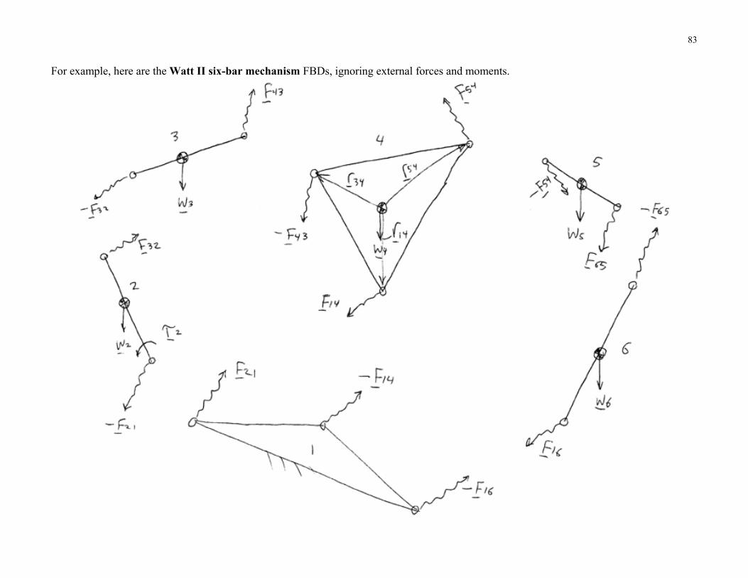
83
For example, here are the Watt II six-bar mechanism FBDs, ignoring external forces and moments.
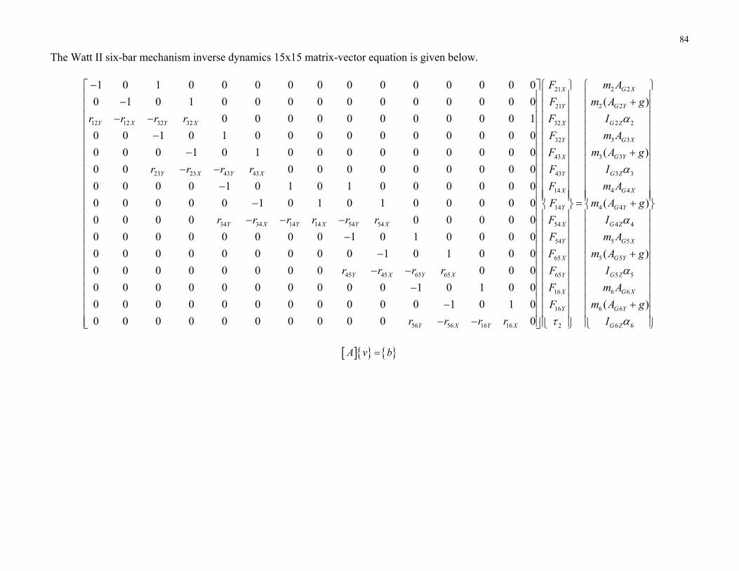
84
The Watt II six-bar mechanism inverse dynamics 15x15 matrix-vector equation is given below.
12 12 32 32
23 23 43 43
34 34 14 14 54 54
1 0 1 0 0 0 0 0 0 0 0 0 0 0 0
0 1 0 1 0 0 0 0 0 0 0 0 0 0 0
0 0 0 0 0 0 0 0 0 0 1
0 0 1 0 1 0 0 0 0 0 0 0 0 0 0
0 0 0 1 0 1 0 0 0 0 0 0 0 0 0
0 0 0 0 0 0 0 0 0 0 0
0 0 0 0 1 0 1 0 1 0 0 0 0 0 0
0 0 0 0 0 1 0 1 0 1 0 0 0 0 0
0 0 0 0 0 0 0 0 0
0 0 0 0 0 0 0 0 1
Y X Y X
Y X Y X
Y X Y X Y X
r r r r
r r r r
r r r r r r
21
21
32
32
43
43
14
14
54
54
45 45 65 65
56 56 16 16
0 1 0 0 0 0
0 0 0 0 0 0 0 0 0 1 0 1 0 0 0
0 0 0 0 0 0 0 0 0 0 0
0 0 0 0 0 0 0 0 0 0 1 0 1 0 0
0 0 0 0 0 0 0 0 0 0 0 1 0 1 0
0 0 0 0 0 0 0 0 0 0 0
X
Y
X
Y
X
Y
X
Y
X
Y
Y X Y X
Y X Y X
F
F
F
F
F
F
F
F
F
F
r r r r
r r r r
2 2
2 2
2 2
3 3
3 3
3 3
4 4
4 4
4 4
5 5
5 565
5 565
6 616
6 616
6 62
( )
( )
( )
( )
( )
G X
G Y
G Z
G X
G Y
G Z
G X
G Y
G Z
G X
G YX
G ZY
G XX
G YY
G Z
m A
m A g
I
m A
m A g
I
m A
m A g
I
m A
m A gF
IF
m AF
m A gF
I
A v b
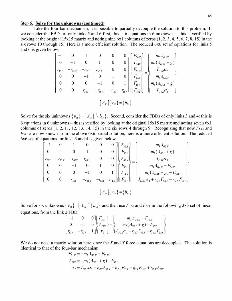
85
Step 6. Solve for the unknowns (continued) Like the four-bar mechanism, it is possible to partially decouple the solution to this problem. If we consider the FBDs of only links 5 and 6 first, this is 6 equations in 6 unknowns – this is verified by looking at the original 15x15 matrix and noting nine 6x1 columns of zeros (1, 2, 3, 4, 5, 6, 7, 8, 15) in the six rows 10 through 15. Here is a more efficient solution. The reduced 6x6 set of equations for links 5 and 6 is given below.
54 5 5
54 5 5
45 45 65 65 65 5 5
65 6 6
16 6 6
56 56 16 16 16 6 6
1 0 1 0 0 0
0 1 0 1 0 0 ( )
0 0
0 0 1 0 1 0
0 0 0 1 0 1 ( )
0 0
X G X
Y G Y
Y X Y X X G Z
Y G X
X G Y
Y X Y X Y G Z
F m A
F m A g
r r r r F I
F m A
F m A g
r r r r F I
56 56 56A v b
Solve for the six unknowns 1
56 56 56v A b . Second, consider the FBDs of only links 3 and 4: this is
6 equations in 6 unknowns – this is verified by looking at the original 15x15 matrix and noting seven 6x1 columns of zeros (1, 2, 11, 12, 13, 14, 15) in the six rows 4 through 9. Recognizing that now F54X and F54Y are now known from the above 6x6 partial solution, here is a more efficient solution. The reduced 6x6 set of equations for links 3 and 4 is given below.
3 332
3 332
23 23 43 43 3 343
4 4 5443
4 4 5414
34 34 14 14 4 4 54 5414
1 0 1 0 0 0
0 1 0 1 0 0 ( )
0 0
0 0 1 0 1 0
0 0 0 1 0 1 ( )
0 0
G XX
G YY
Y X Y X G ZX
G X XY
G Y YX
Y X Y X G Z Y XY
m AF
m A gF
r r r r IF
m A FF
m A g FF
r r r r I r F rF
54 54X YF
34 34 34A v b
Solve for six unknowns 1
34 34 34v A b and then use F32X and F32Y in the following 3x3 set of linear
equations, from the link 2 FBD.
21 2 2 32
21 2 2 32
12 12 2 2 2 32 32 32 32
1 0 0
0 1 0 ( )
1
X G X X
Y G Y Y
Y X G Z Y X X Y
F m A F
F m A g F
r r I r F r F
We do not need a matrix solution here since the X and Y force equations are decoupled. The solution is identical to that of the four-bar mechanism.
21 2 2 32
21 2 2 32
2 2 2 32 32 32 32 12 21 12 21
( )X G X X
Y G Y Y
G Z Y X X Y Y X X Y
F m A F
F m A g F
I r F r F r F r F

86
Matrix inversion requires approximately 33
log
n
n and Gaussian elimination requires approximately
22( 1)
3
n nn
multiplications/divisions (Nering, 1974).
Number of Multiplications/Divisions
Method Inversion Gaussian Reduction
15x15 8609 1345 84% 6x6 twice, plus decoupled link 2 1672 183 89% Reduction in cost 81% 86%
There is an astonishing 86% reduction in computational cost for Gaussian elimination with the methods using 6x6 inversion twice, plus the decoupled link 2 solution. Also, the numerical accuracy may also improve with this method since we needn’t do unnecessary calculations with the sixteen 6x1 columns of zeros. Any mechanism with a dyad of binary links may be decoupled in this manner. Thus, the method is similar and the computational complexity identical for the Stephenson I, Stephenson III, Watt I, and Watt II six-bar mechanisms. The Stephenson II six-bar mechanism does not include a dyad of binary links and so it cannot be solved like the other 4 six-bar mechanisms (first links 5 and 6, then links 3 and 4 with one unknown vector force from 5 and 6, then link 2 independently). But links 3, 4, 5, and 6 can be solved first independently of link 2: a 12x12 solution followed by the standard link 2 solution. The computational savings is not as impressive as in the former six-bar cases.
Number of Multiplications/Divisions, Stephenson II Six-Bar
Method Inversion Gaussian Reduction 15x15 8609 1345 84% 12x12 plus decoupled link 2 4811 723 85% Reduction in cost 44% 46%
There is a 46% reduction in computational cost for Gaussian elimination with the 12x12 plus decoupled link 2 method. Also, the numerical accuracy may also improve with this method since we needn’t do unnecessary calculations with the three 12x1 columns of zeros.
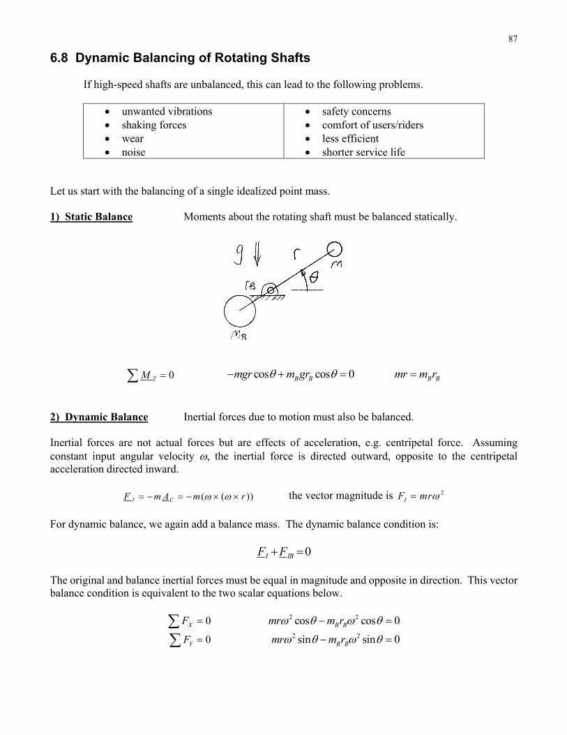
87
6.8 Dynamic Balancing of Rotating Shafts If high-speed shafts are unbalanced, this can lead to the following problems.
unwanted vibrations shaking forces wear noise
safety concerns comfort of users/riders less efficient shorter service life
Let us start with the balancing of a single idealized point mass. 1) Static Balance Moments about the rotating shaft must be balanced statically.
0ZM cos cos 0B Bmgr m gr B Bmr m r
2) Dynamic Balance Inertial forces due to motion must also be balanced. Inertial forces are not actual forces but are effects of acceleration, e.g. centripetal force. Assuming constant input angular velocity , the inertial force is directed outward, opposite to the centripetal acceleration directed inward.
( ( ))I CF m A m r the vector magnitude is 2IF mr
For dynamic balance, we again add a balance mass. The dynamic balance condition is:
0I IBF F
The original and balance inertial forces must be equal in magnitude and opposite in direction. This vector balance condition is equivalent to the two scalar equations below.
0
0
X
Y
F
F
2 2
2 2
cos cos 0
sin sin 0
B B
B B
mr m r
mr m r
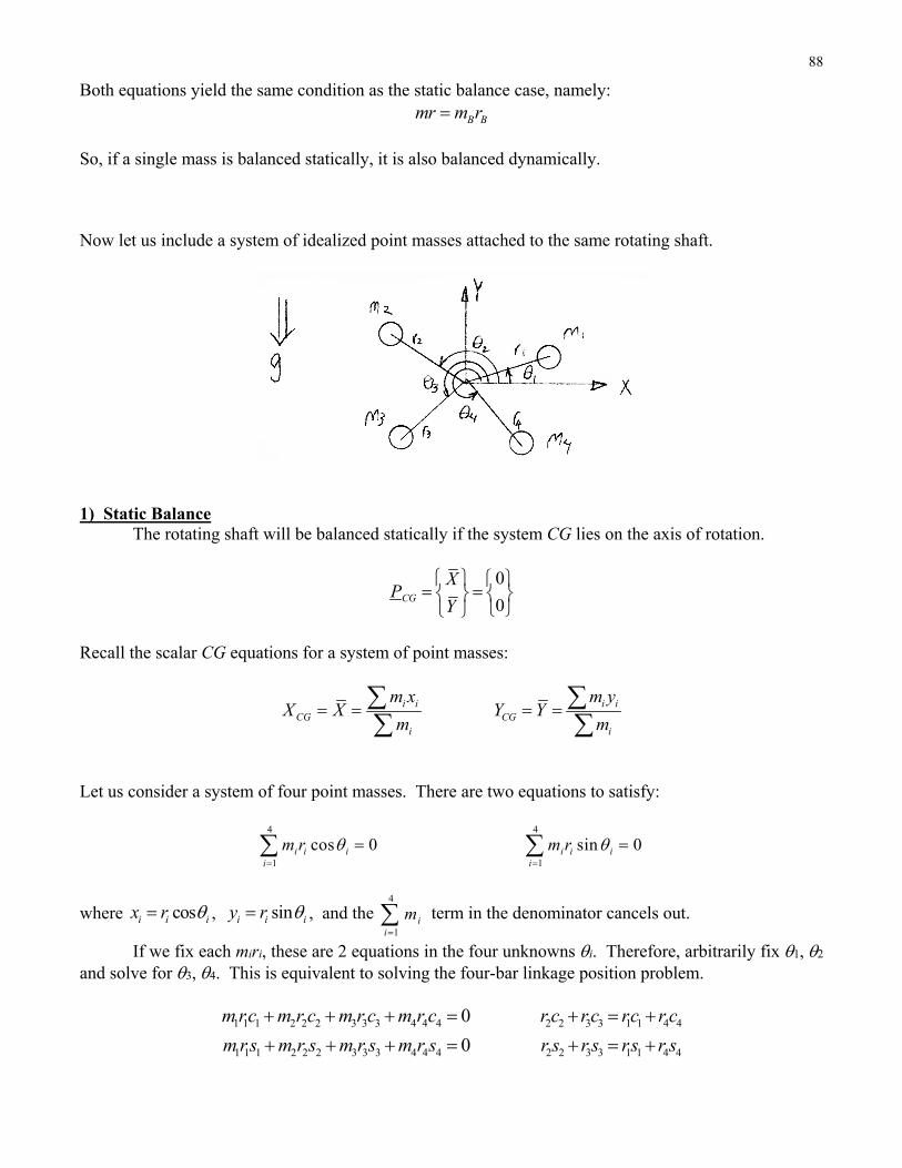
88
Both equations yield the same condition as the static balance case, namely:
B Bmr m r
So, if a single mass is balanced statically, it is also balanced dynamically. Now let us include a system of idealized point masses attached to the same rotating shaft.
1) Static Balance The rotating shaft will be balanced statically if the system CG lies on the axis of rotation.
0
0CG
XP
Y
Recall the scalar CG equations for a system of point masses:
i iCG
i
m xX X
m
i i
CGi
m yY Y
m
Let us consider a system of four point masses. There are two equations to satisfy:
4
1
cos 0i i ii
m r
4
1
sin 0i i ii
m r
where cosi i ix r , sini i iy r , and the 4
1i
i
m term in the denominator cancels out.
If we fix each miri, these are 2 equations in the four unknowns i. Therefore, arbitrarily fix 1,2 and solve for 3,4. This is equivalent to solving the four-bar linkage position problem.
1 1 1 2 2 2 3 3 3 4 4 4
1 1 1 2 2 2 3 3 3 4 4 4
0
0
m rc m r c m r c m r c
m rs m r s m r s m r s
2 2 3 3 1 1 4 4
2 2 3 3 1 1 4 4
r c r c rc r c
r s r s rs r s
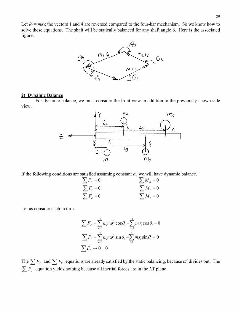
89
Let Ri = miri; the vectors 1 and 4 are reversed compared to the four-bar mechanism. So we know how to solve these equations. The shaft will be statically balanced for any shaft angle . Here is the associated figure.
2) Dynamic Balance For dynamic balance, we must consider the front view in addition to the previously-shown side view.
If the following conditions are satisfied assuming constant , we will have dynamic balance.
0
0
0
X
Y
Z
F
F
F
0
0
0
X
Y
Z
M
M
M
Let us consider each in turn.
4 42
1 1
4 42
1 1
cos cos 0
sin sin 0
0 0
X i i i i i ii i
Y i i i i i ii i
Z
F m r m r
F m r m r
F
The XF and YF equations are already satisfied by the static balancing, because 2 divides out. The
ZF equation yields nothing because all inertial forces are in the XY plane.
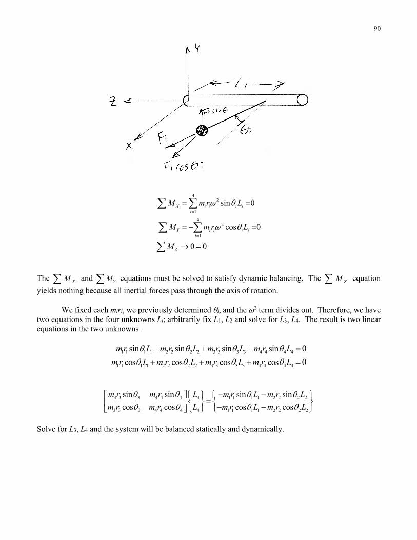
90
42
1
42
1
sin 0
cos 0
0 0
X i i i ii
Y i i i ii
Z
M m r L
M m r L
M
The XM and YM equations must be solved to satisfy dynamic balancing. The ZM equation
yields nothing because all inertial forces pass through the axis of rotation. We fixed each miri, we previously determined i, and the 2 term divides out. Therefore, we have two equations in the four unknowns Li; arbitrarily fix L1, L2 and solve for L3, L4. The result is two linear equations in the two unknowns.
1 1 1 1 2 2 2 2 3 3 3 3 4 4 4 4
1 1 1 1 2 2 2 2 3 3 3 3 4 4 4 4
sin sin sin sin 0
cos cos cos cos 0
m r L m r L m r L m r L
m r L m r L m r L m r L
3 3 3 4 4 4 3 1 1 1 1 2 2 2 2
3 3 3 4 4 4 4 1 1 1 1 2 2 2 2
sin sin sin sin
cos cos cos cos
m r m r L m r L m r L
m r m r L m r L m r L
Solve for L3, L4 and the system will be balanced statically and dynamically.
91
7. Gears and Cams 7.1 Gears 7.1.3 Gear Trains To obtain a higher gear ratio than practical with a single pair of standard involute spur gears, one can mate any number of spur gears in a gearbox, or gear train. The leftmost gear is the driving gear and the rightmost is the output gear. All intermediate gears are first the driven gear and then the driving gear as we proceed from left to right. Let us calculate the overall gear ratio nGT.
INGT
OUT
n
Example We can find the overall gear ratio by canceling neighboring intermediate angular velocities. Each term in the above product may be replaced by its known number of teeth ratio. All intermediate ratios cancel, so We could have done the same with pitch radii instead of number of teeth because they are in direct proportion. So, the intermediate gears are idlers. Their number of teeth effect cancels out, but they do change direction. We should have included the +/– signs, by inspection. For gear trains composed of externally-meshing spur gear pairs:
odd number of gears the output is in the same direction as the input even number of gears the output is in the opposite direction as the input

92
Improved gear train That gear train concept did not work. Now let us mate any number of spur gears, where the driving and driven gears are distinct, because each pair is rigidly attached to the same shaft. Again, let us calculate the overall gear ratio.
INGT
OUT
n
Example Again, we use the equation But now the gears rigidly attached to the same shaft have the same angular velocity ratio, so The general formula for this case is Again, we must consider direction For gear trains composed of externally-meshing spur gear pairs:
odd number of pairs the output is in the opposite direction as the input even number of pairs the output is in the same direction as the input
93
7.1.4 Involute Spur Gear Standardization Rolling Cylinders Mating spur gears are based on two pitch circles rolling without slip. These are fictitious circles, i.e. you cannot look on a gear to see them. The actual gear teeth both roll and slide with respect to each other (via the two-dof gear joint). Fundamental Law of Gearing The angular velocity between the gears of a gearset must remain constant throughout the mesh. From our study of linkage velocity, we know this is no easy feat. Velocity ratios in a linkage vary wildly over the range of motion.
Velocity Ratio 1
VR OUT IN
IN OUT
r
r n
Torque Ratio TR IN OUT
OUT IN
rn
r
The velocity ratio is the inverse of the gear ratio n and the torque ratio is the same as the gear ratio n defined previously. The torque ratio is also called Mechanical Advantage (MA). Involute Function Standard spur gears have an involute tooth shape. If the gears’ center distance is not perfect (tolerances, thermal expansion, wear – in design the center distance is increased slightly by the engineer to allow for these effects; this is called clearance), the angular velocity ratio will still be constant to satisfy the Fundamental Law of Gearing.

94
The involute of a circle is a curve generated by unwrapping a taut sting from the circumference of a so-called base circle, always keeping it tangent to the circle. The figure below has th = [0:5:60]*DR and rb = 1 m. The red circle is the gear base circle, the blue lines are the taut tangent construction lines, and the green curve is the involute function.
Involute Function Construction
In polar coordinates (, r), the parametric equations for the involute of a circle are given below.
tan
secb
t t
r r t
where t is the independent parameter and rb is the base circle radius. In Cartesian coordinates (xI, yI):
cos sec cos(tan )
sin sec sin(tan )I b
I b
x r r t t t
y r r t t t
-1 -0.5 0 0.5 1 1.5
-1
-0.5
0
0.5
1
X (m)
Y (
m)
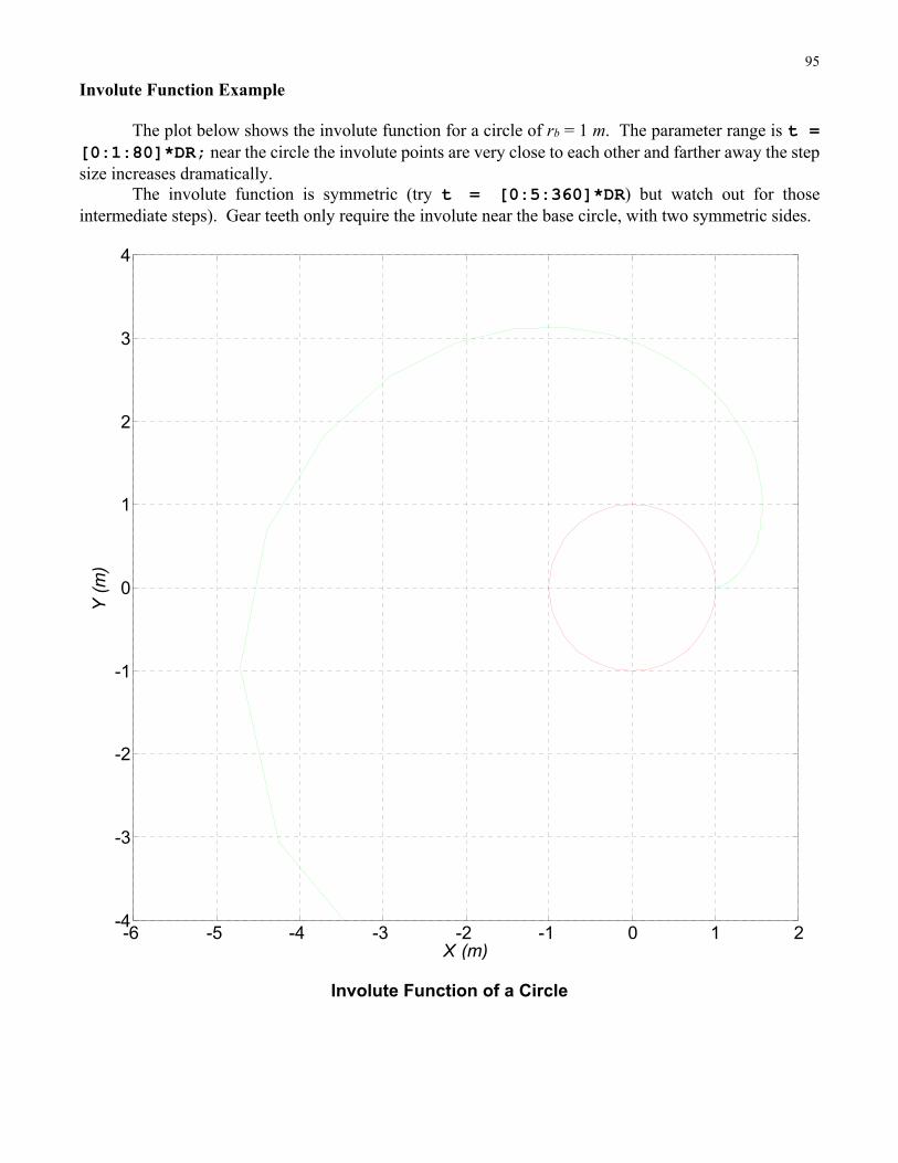
95
Involute Function Example The plot below shows the involute function for a circle of rb = 1 m. The parameter range is t = [0:1:80]*DR; near the circle the involute points are very close to each other and farther away the step size increases dramatically. The involute function is symmetric (try t = [0:5:360]*DR) but watch out for those intermediate steps). Gear teeth only require the involute near the base circle, with two symmetric sides.
Involute Function of a Circle
-6 -5 -4 -3 -2 -1 0 1 2-4
-3
-2
-1
0
1
2
3
4
X (m)
Y (
m)
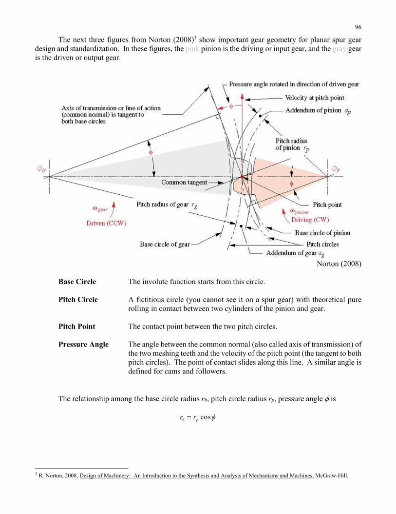
96
The next three figures from Norton (2008)3 show important gear geometry for planar spur gear design and standardization. In these figures, the pink pinion is the driving or input gear, and the gray gear is the driven or output gear.
Norton (2008)
Base Circle The involute function starts from this circle.
Pitch Circle A fictitious circle (you cannot see it on a spur gear) with theoretical pure rolling in contact between two cylinders of the pinion and gear.
Pitch Point The contact point between the two pitch circles.
Pressure Angle The angle between the common normal (also called axis of transmission) of the two meshing teeth and the velocity of the pitch point (the tangent to both pitch circles). The point of contact slides along this line. A similar angle is defined for cams and followers.
The relationship among the base circle radius rb, pitch circle radius rp, pressure angle is
cosb pr r
3 R. Norton, 2008, Design of Machinery: An Introduction to the Synthesis and Analysis of Mechanisms and Machines, McGraw-Hill.

97
Norton (2008)
The length of contact is measured along the axis of transmission. The beginning of contact is when the tip of the driven gear tooth intersects the axis of transmission. The end of contact is when the tip of driving gear tooth intersects the axis of transmission, as shown in the figure above. Only one or two teeth are in contact at any one time for standard spur gears.
For harmonic gearing, many teeth are in contact at any one time, which provides a higher gear ratio in a smaller package.
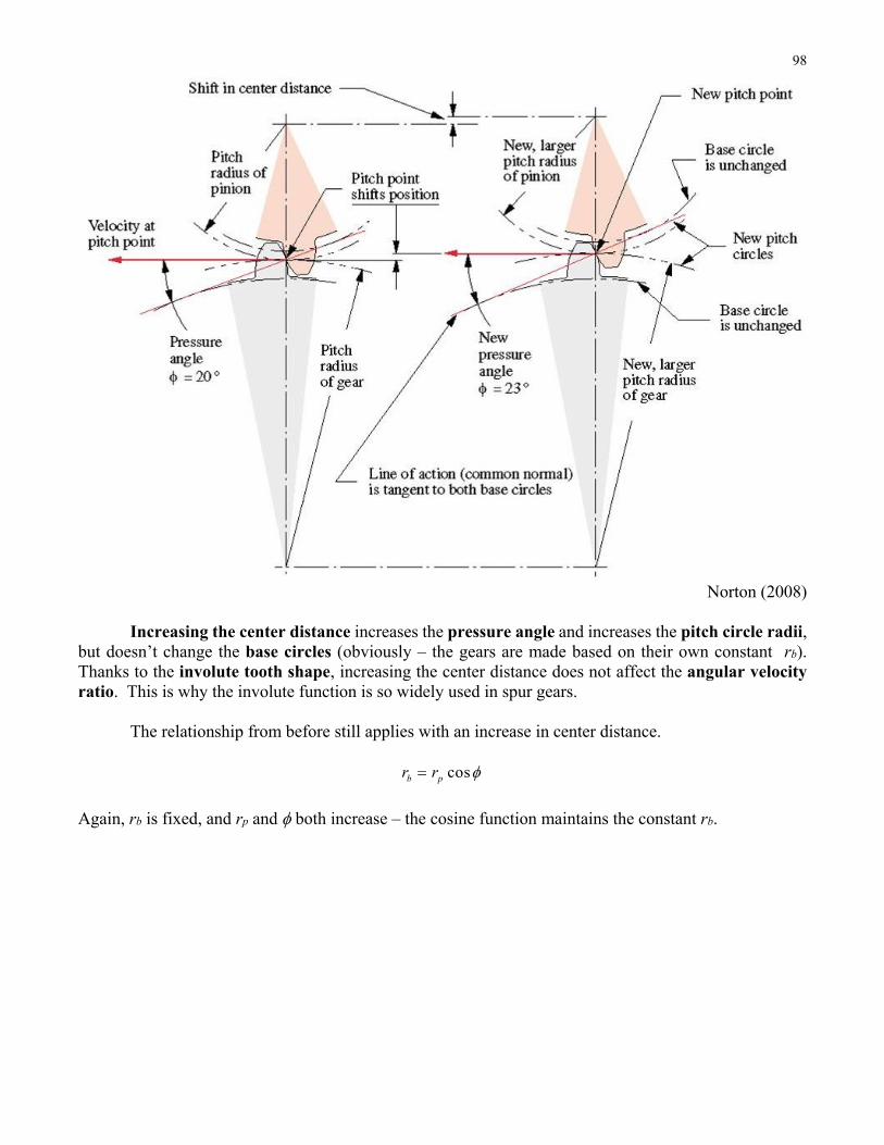
98
Norton (2008)
Increasing the center distance increases the pressure angle and increases the pitch circle radii, but doesn’t change the base circles (obviously – the gears are made based on their own constant rb). Thanks to the involute tooth shape, increasing the center distance does not affect the angular velocity ratio. This is why the involute function is so widely used in spur gears. The relationship from before still applies with an increase in center distance.
cosb pr r
Again, rb is fixed, and rp and both increase – the cosine function maintains the constant rb.

99
Spur Gear Standardization Gear standardization is used to allow interchangeability in manufacturing and to allow meshing of different size gears (different pitch radii and number of teeth) to achieve desired gear ratios. For two spur gears to mesh, they must have
1) the same pressure angle (see previous figures and definition) 2) the same diametral pitch (see the equation below) 3) standard tooth proportions (see the figure below)
diametral pitch d
Np
d
Where N is the number of teeth and d is the pitch diameter, both for each gear.
module 1
d
dm
N p
Module is the SI version of diametral pitch (it is the inverse). SI gears are not interchangeable with English system gears because of different tooth proportion standards.
circular pitch c
dp
N
Circular pitch is the circumferential distance (arc length) between teeth along the pitch circle of a spur gear.
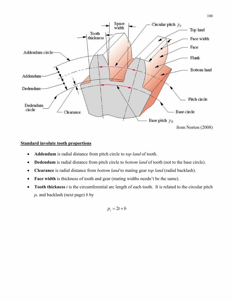
100
from Norton (2008)
Standard involute tooth proportions
Addendum is radial distance from pitch circle to top land of tooth.
Dedendum is radial distance from pitch circle to bottom land of tooth (not to the base circle).
Clearance is radial distance from bottom land to mating gear top land (radial backlash).
Face width is thickness of tooth and gear (mating widths needn’t be the same).
Tooth thickness t is the circumferential arc length of each tooth. It is related to the circular pitch
pc and backlash (next page) b by
2cp t b
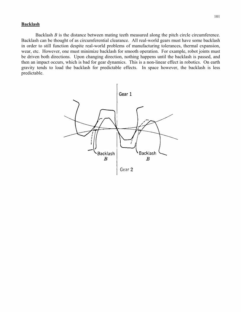
101
Backlash
Backlash B is the distance between mating teeth measured along the pitch circle circumference. Backlash can be thought of as circumferential clearance. All real-world gears must have some backlash in order to still function despite real-world problems of manufacturing tolerances, thermal expansion, wear, etc. However, one must minimize backlash for smooth operation. For example, robot joints must be driven both directions. Upon changing direction, nothing happens until the backlash is passed, and then an impact occurs, which is bad for gear dynamics. This is a non-linear effect in robotics. On earth gravity tends to load the backlash for predictable effects. In space however, the backlash is less predictable.
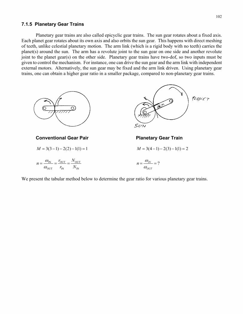
102
7.1.5 Planetary Gear Trains Planetary gear trains are also called epicyclic gear trains. The sun gear rotates about a fixed axis. Each planet gear rotates about its own axis and also orbits the sun gear. This happens with direct meshing of teeth, unlike celestial planetary motion. The arm link (which is a rigid body with no teeth) carries the planet(s) around the sun. The arm has a revolute joint to the sun gear on one side and another revolute joint to the planet gear(s) on the other side. Planetary gear trains have two-dof, so two inputs must be given to control the mechanism. For instance, one can drive the sun gear and the arm link with independent external motors. Alternatively, the sun gear may be fixed and the arm link driven. Using planetary gear trains, one can obtain a higher gear ratio in a smaller package, compared to non-planetary gear trains.
Conventional Gear Pair Planetary Gear Train 3(3 1) 2(2) 1(1) 1M 3(4 1) 2(3) 1(1) 2M
IN OUT OUT
OUT IN IN
r Nn
r N
?IN
OUT
n
We present the tabular method below to determine the gear ratio for various planetary gear trains.
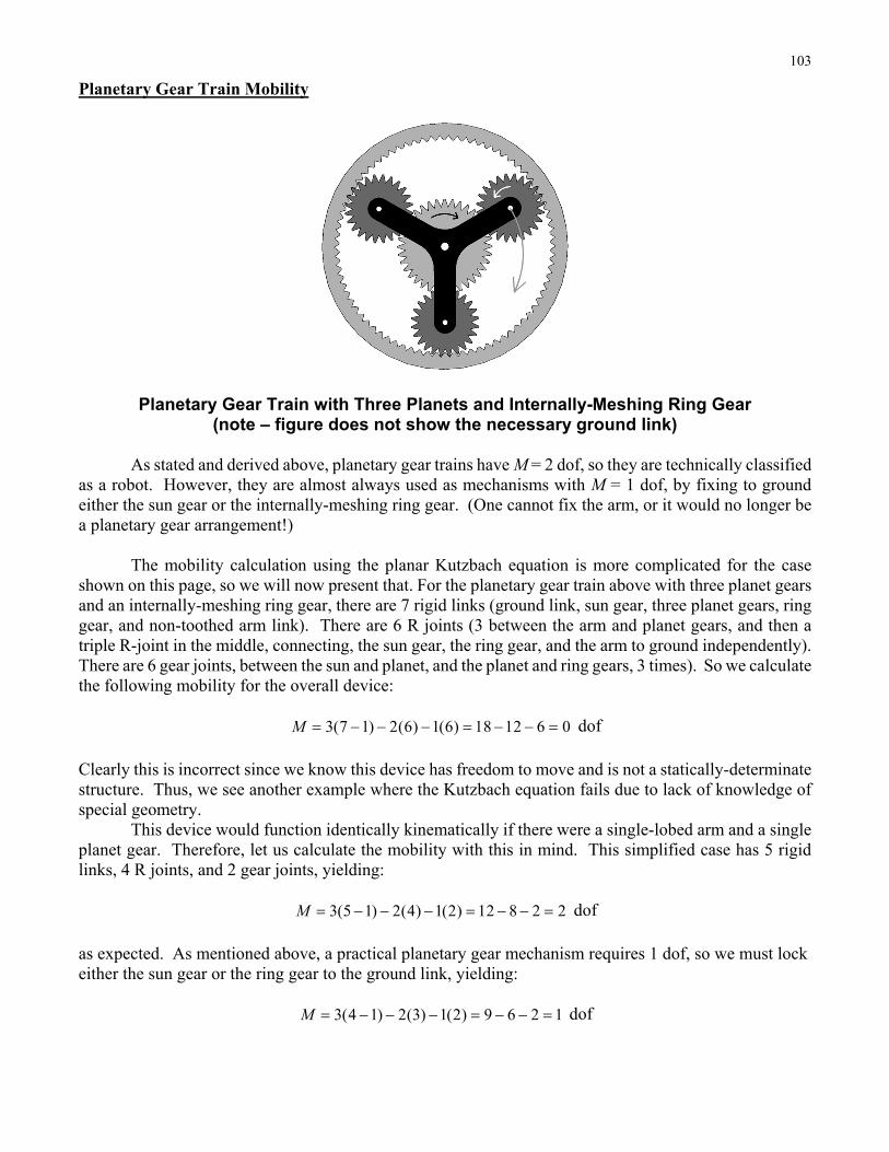
103
Planetary Gear Train Mobility
Planetary Gear Train with Three Planets and Internally-Meshing Ring Gear (note – figure does not show the necessary ground link)
As stated and derived above, planetary gear trains have M = 2 dof, so they are technically classified
as a robot. However, they are almost always used as mechanisms with M = 1 dof, by fixing to ground either the sun gear or the internally-meshing ring gear. (One cannot fix the arm, or it would no longer be a planetary gear arrangement!)
The mobility calculation using the planar Kutzbach equation is more complicated for the case
shown on this page, so we will now present that. For the planetary gear train above with three planet gears and an internally-meshing ring gear, there are 7 rigid links (ground link, sun gear, three planet gears, ring gear, and non-toothed arm link). There are 6 R joints (3 between the arm and planet gears, and then a triple R-joint in the middle, connecting, the sun gear, the ring gear, and the arm to ground independently). There are 6 gear joints, between the sun and planet, and the planet and ring gears, 3 times). So we calculate the following mobility for the overall device:
3(7 1) 2(6) 1(6) 18 12 6 0M dof Clearly this is incorrect since we know this device has freedom to move and is not a statically-determinate structure. Thus, we see another example where the Kutzbach equation fails due to lack of knowledge of special geometry. This device would function identically kinematically if there were a single-lobed arm and a single planet gear. Therefore, let us calculate the mobility with this in mind. This simplified case has 5 rigid links, 4 R joints, and 2 gear joints, yielding:
3(5 1) 2(4) 1(2) 12 8 2 2M dof as expected. As mentioned above, a practical planetary gear mechanism requires 1 dof, so we must lock either the sun gear or the ring gear to the ground link, yielding:
3(4 1) 2(3) 1(2) 9 6 2 1M dof
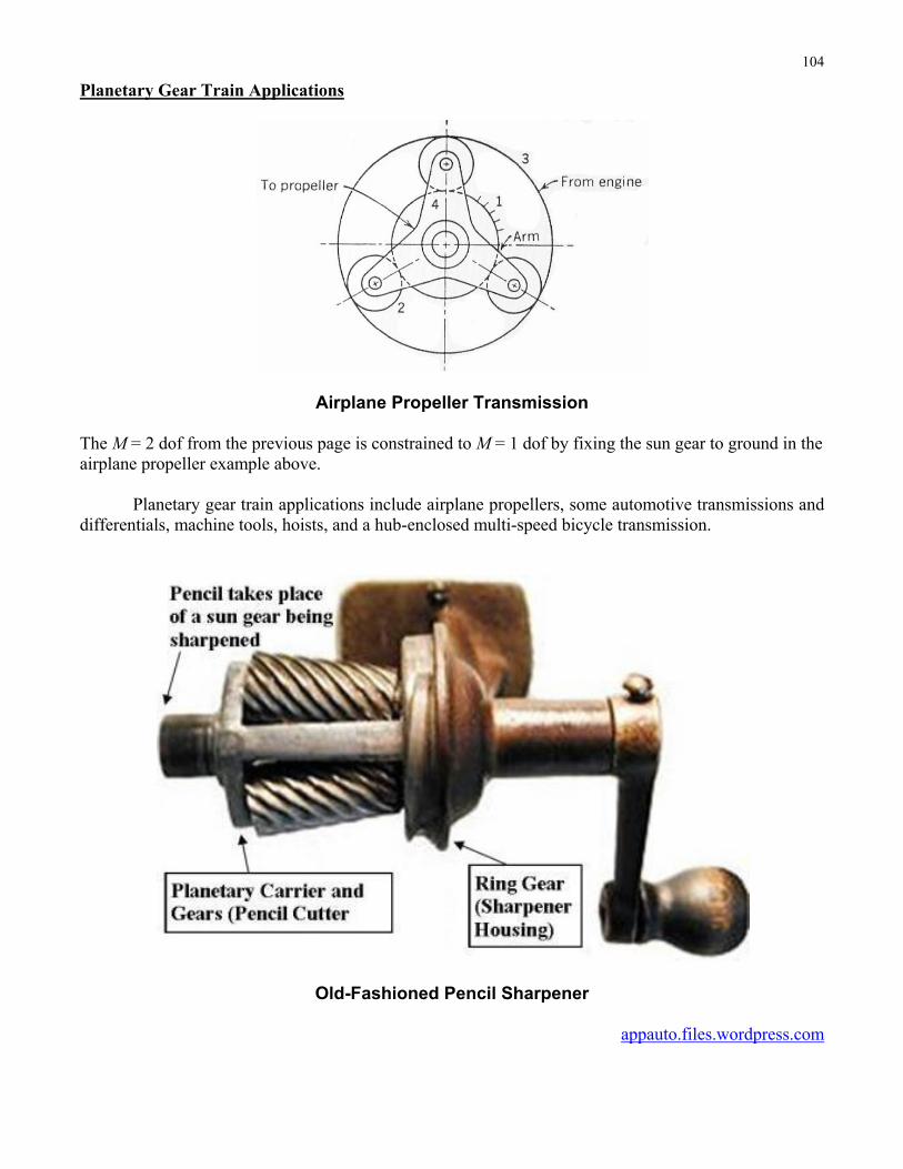
104
Planetary Gear Train Applications
Airplane Propeller Transmission The M = 2 dof from the previous page is constrained to M = 1 dof by fixing the sun gear to ground in the airplane propeller example above. Planetary gear train applications include airplane propellers, some automotive transmissions and differentials, machine tools, hoists, and a hub-enclosed multi-speed bicycle transmission.
Old-Fashioned Pencil Sharpener
appauto.files.wordpress.com
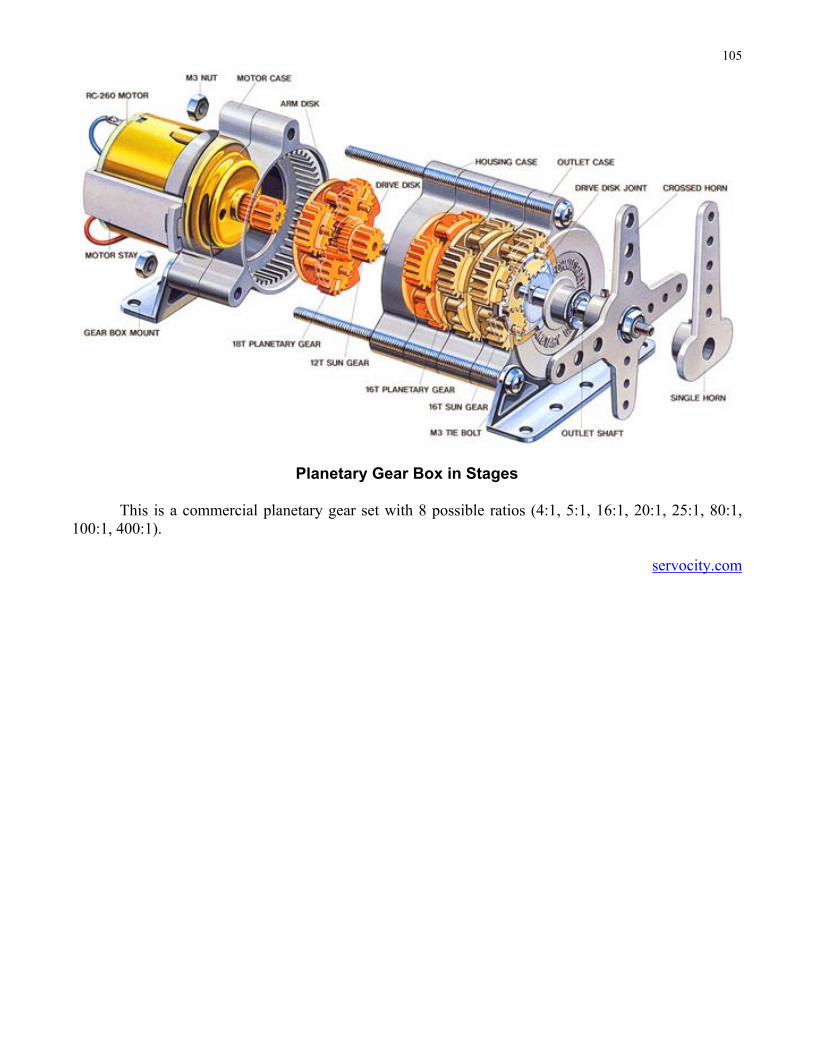
105
Planetary Gear Box in Stages
This is a commercial planetary gear set with 8 possible ratios (4:1, 5:1, 16:1, 20:1, 25:1, 80:1, 100:1, 400:1).
servocity.com
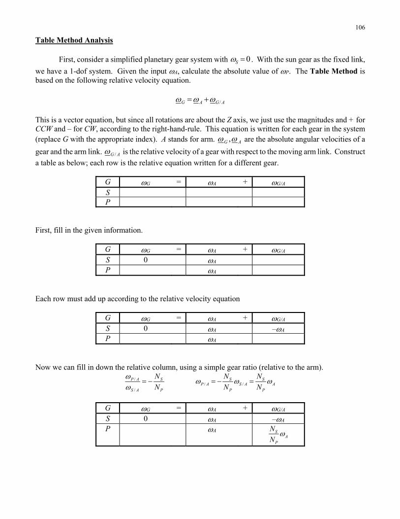
106
Table Method Analysis First, consider a simplified planetary gear system with 0S . With the sun gear as the fixed link,
we have a 1-dof system. Given the input A, calculate the absolute value of P. The Table Method is based on the following relative velocity equation.
/G A G A
This is a vector equation, but since all rotations are about the Z axis, we just use the magnitudes and + for CCW and – for CW, according to the right-hand-rule. This equation is written for each gear in the system (replace G with the appropriate index). A stands for arm. ,G A are the absolute angular velocities of a
gear and the arm link. /G A is the relative velocity of a gear with respect to the moving arm link. Construct
a table as below; each row is the relative equation written for a different gear.
G G = A + G/A S P
First, fill in the given information.
G G = A + G/A S 0 A P A
Each row must add up according to the relative velocity equation
G G = A + G/A S 0 A –A P A
Now we can fill in down the relative column, using a simple gear ratio (relative to the arm).
/
/
P A S
S A P
N
N
/ /S S
P A S A AP P
N N
N N
G G = A + G/A S 0 A –A P A S
AP
N
N
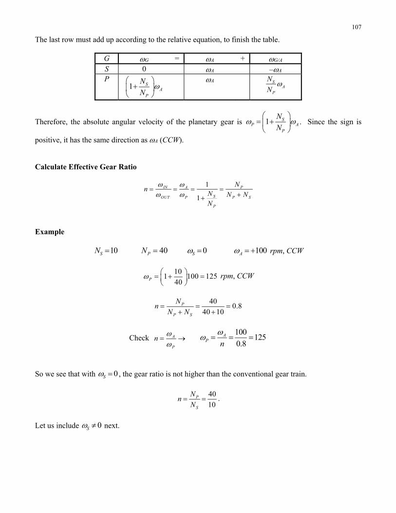
107
The last row must add up according to the relative equation, to finish the table.
G G = A + G/A S 0 A –A P
1 SA
P
N
N
A SA
P
N
N
Therefore, the absolute angular velocity of the planetary gear is 1 SP A
P
N
N
. Since the sign is
positive, it has the same direction as A (CCW). Calculate Effective Gear Ratio
1
1
IN A P
SOUT P P S
P
Nn
N N NN
Example
10SN 40PN 0S 100A rpm, CCW
10
1 100 12540P
rpm, CCW
40
0.840 10
P
P S
Nn
N N
Check A
P
n
100
1250.8
AP n
So we see that with 0S , the gear ratio is not higher than the conventional gear train.
40
10P
S
Nn
N .
Let us include 0S next.
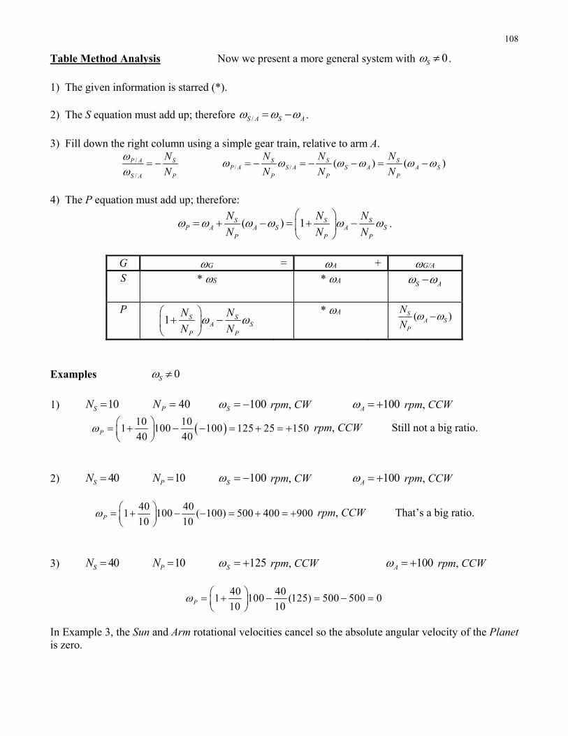
108
Table Method Analysis Now we present a more general system with 0S .
1) The given information is starred (*). 2) The S equation must add up; therefore /S A S A .
3) Fill down the right column using a simple gear train, relative to arm A.
/
/
P A S
S A P
N
N
/ / ( ) ( )S S SP A S A S A A S
P P P
N N N
N N N
4) The P equation must add up; therefore:
( ) 1S S SP A A S A S
P P P
N N N
N N N
.
G G = A + G/A S * S * A
S A
P
1 S SA S
P P
N N
N N
* A ( )S
A SP
N
N
Examples 0S
1) 10SN 40PN 100S rpm, CW 100A rpm, CCW
10 101 100 100 125 25 150
40 40P
rpm, CCW Still not a big ratio.
2) 40SN 10PN 100S rpm, CW 100A rpm, CCW
40 401 100 ( 100) 500 400 900
10 10P
rpm, CCW That’s a big ratio.
3) 40SN 10PN 125S rpm, CCW 100A rpm, CCW
40 401 100 (125) 500 500 0
10 10P
In Example 3, the Sun and Arm rotational velocities cancel so the absolute angular velocity of the Planet is zero.
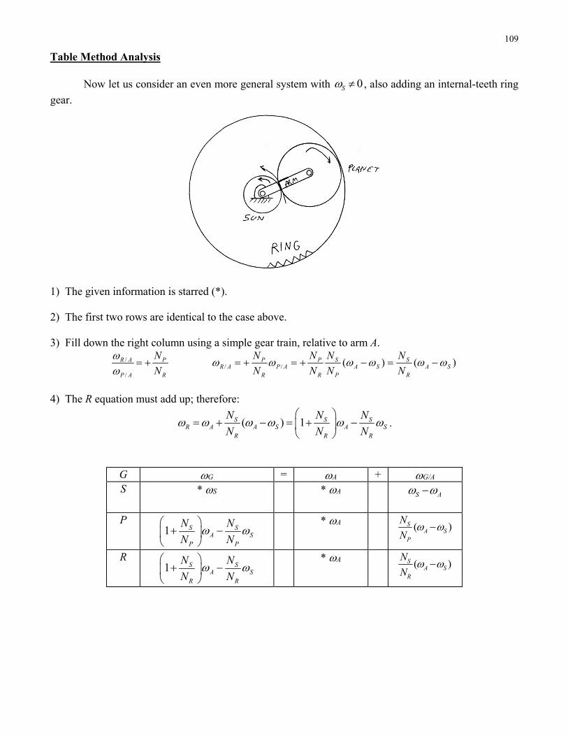
109
Table Method Analysis Now let us consider an even more general system with 0S , also adding an internal-teeth ring
gear.
1) The given information is starred (*). 2) The first two rows are identical to the case above. 3) Fill down the right column using a simple gear train, relative to arm A.
/
/
R A P
P A R
N
N
/ / ( ) ( )S SP PR A P A A S A S
R R P R
N NN N
N N N N
4) The R equation must add up; therefore:
( ) 1S S SR A A S A S
R R R
N N N
N N N
.
G G = A + G/A S * S * A
S A
P
1 S SA S
P P
N N
N N
* A ( )S
A SP
N
N
R 1 S S
A SR R
N N
N N
* A ( )S
A SR
N
N
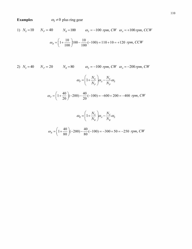
110
Examples 0S plus ring gear
1) 10SN 40PN 100RN 100S rpm, CW 100A rpm, CCW
10 10
1 100 ( 100) 110 10 120100 100R
rpm, CCW
2) 40SN 20PN 80RN 100S rpm, CW 200A rpm, CW
1 S SP A S
P P
N N
N N
40 40
1 ( 200) ( 100) 600 200 40020 20P
rpm, CW
1 S SR A S
R R
N N
N N
40 40
1 ( 200) ( 100) 300 50 25080 80R
rpm, CW
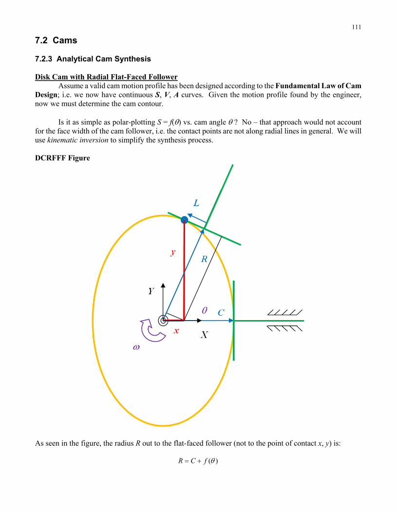
111
7.2 Cams 7.2.3 Analytical Cam Synthesis Disk Cam with Radial Flat-Faced Follower Assume a valid cam motion profile has been designed according to the Fundamental Law of Cam Design; i.e. we now have continuous S, V, A curves. Given the motion profile found by the engineer, now we must determine the cam contour.
Is it as simple as polar-plotting S = f() vs. cam angle ? No – that approach would not account for the face width of the cam follower, i.e. the contact points are not along radial lines in general. We will use kinematic inversion to simplify the synthesis process. DCRFFF Figure
As seen in the figure, the radius R out to the flat-faced follower (not to the point of contact x, y) is:
( )R C f

112
where C is the minimum cam radius, a design variable, and S = f() is the given cam motion profile. The radius R and the flat-faced follower length L can be related to the contact point x, y and the cam angle through geometry.
cos sin
sin cos
R x y
L x y
Notice that
sin cosdR
x y Ld
( ( ))d df
L C fd d
To calculate the follower flat-face length, double the maximum of L from above. It is doubled because by symmetry the contact point will change to the other side at 180 . To summarize thus far:
( )R C f df
Ld
This is sufficient to manufacture the cam since it is machined with , R, L coordinates. If we want to know the cam contour in Cartesian coordinates, we must solve the relationships for x, y. In matrix form:
cos sin
sin cos
x R
y L
This special coefficient matrix [A] is orthonormal, which means both columns and rows are perpendicular to each other and both columns and rows are unit vectors. One unique property of orthonormal matrices
is 1 TA A
. The Cartesian cam contour solution is thus:
cos sin cos sin
sin cos sin cos
x R R L
y L R L
( )cos sin
( )sin cos
dfx C f
d
dfy C f
d
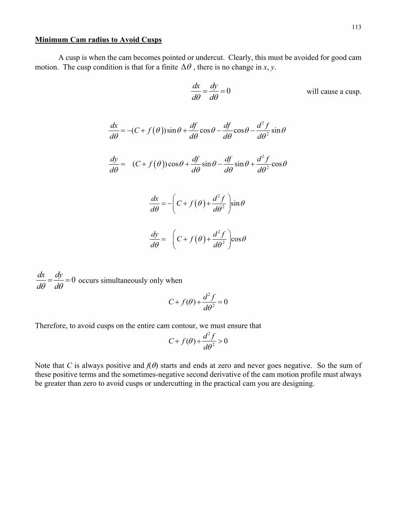
113
Minimum Cam radius to Avoid Cusps A cusp is when the cam becomes pointed or undercut. Clearly, this must be avoided for good cam motion. The cusp condition is that for a finite , there is no change in x, y.
0dx dy
d d will cause a cusp.
2
2
2
2
( )sin cos cos sin
( ) cos sin sin cos
dx df df d fC f
d d d d
dy df df d fC f
d d d d
2
2
2
2
sin
cos
dx d fC f
d d
dy d fC f
d d
0dx dy
d d occurs simultaneously only when
2
2( ) 0
d fC f
d
Therefore, to avoid cusps on the entire cam contour, we must ensure that
2
2( ) 0
d fC f
d
Note that C is always positive and f() starts and ends at zero and never goes negative. So the sum of these positive terms and the sometimes-negative second derivative of the cam motion profile must always be greater than zero to avoid cusps or undercutting in the practical cam you are designing.
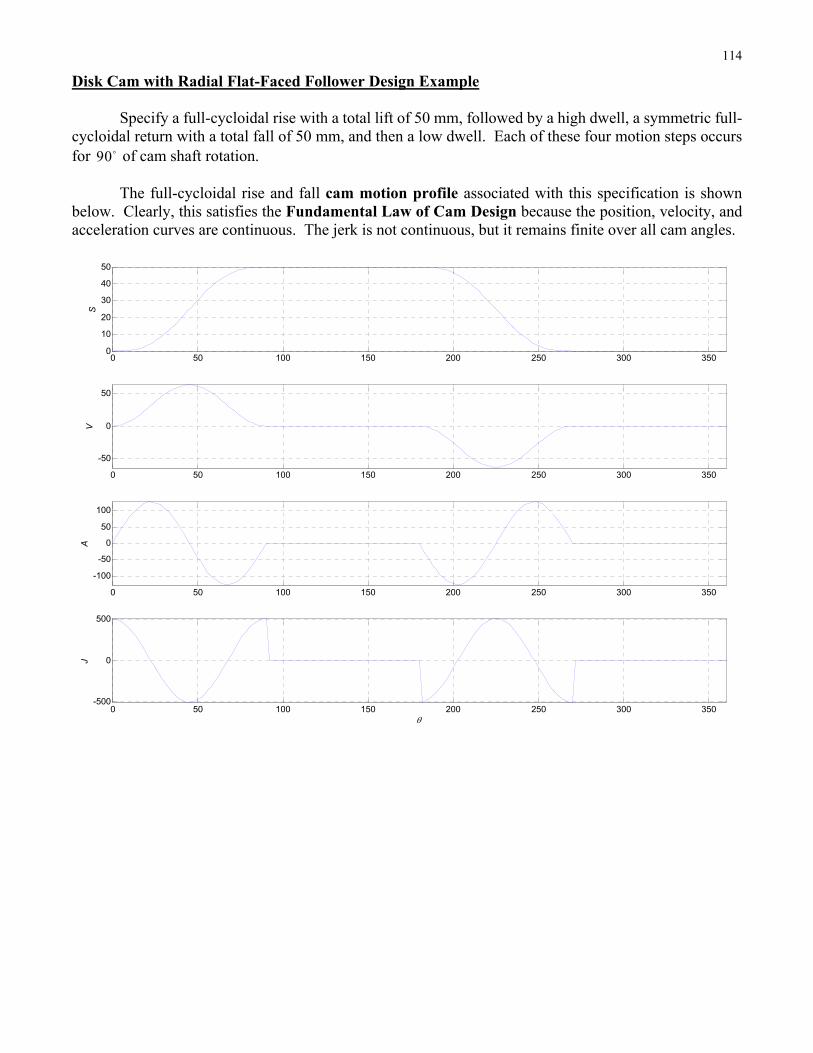
114
Disk Cam with Radial Flat-Faced Follower Design Example Specify a full-cycloidal rise with a total lift of 50 mm, followed by a high dwell, a symmetric full-cycloidal return with a total fall of 50 mm, and then a low dwell. Each of these four motion steps occurs for 90 of cam shaft rotation. The full-cycloidal rise and fall cam motion profile associated with this specification is shown below. Clearly, this satisfies the Fundamental Law of Cam Design because the position, velocity, and acceleration curves are continuous. The jerk is not continuous, but it remains finite over all cam angles.
0 50 100 150 200 250 300 3500
10
20
30
40
50
S
0 50 100 150 200 250 300 350
-50
0
50
V
0 50 100 150 200 250 300 350
-100
-50
0
50
100
A
0 50 100 150 200 250 300 350-500
0
500
J
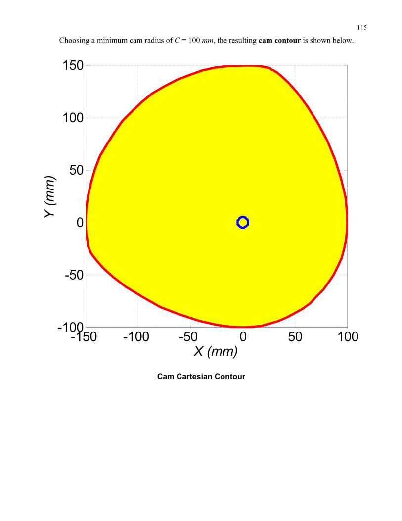
115
Choosing a minimum cam radius of C = 100 mm, the resulting cam contour is shown below.
Cam Cartesian Contour
-150 -100 -50 0 50 100-100
-50
0
50
100
150
X (mm)
Y (
mm
)
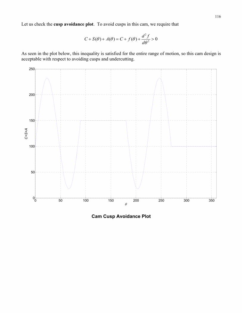
116
Let us check the cusp avoidance plot. To avoid cusps in this cam, we require that
2
2( ) ( ) ( ) 0
d fC S A C f
d
As seen in the plot below, this inequality is satisfied for the entire range of motion, so this cam design is acceptable with respect to avoiding cusps and undercutting.
Cam Cusp Avoidance Plot
0 50 100 150 200 250 300 3500
50
100
150
200
250
C+
S+
A
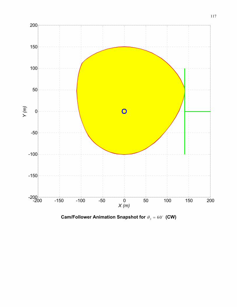
117
Cam/Follower Animation Snapshot for 2 60 (CW)
-200 -150 -100 -50 0 50 100 150 200-200
-150
-100
-50
0
50
100
150
200
X (m)
Y (
m)