On Learning Powers of Poisson Binomial Distributions and ... · On Learning Powers of Poisson...

On Learning Powers of Poisson Binomial

Distributions and Graph Binomial Distributions

Dimitris Fotakis

Yahoo Research NY and National Technical University of Athens

Joint work with Vasilis Kontonis (NTU Athens),

Piotr Krysta (Liverpool) and Paul Spirakis (Liverpool and Patras)

Distribution Learning

• Draw samples from unknown distribution P (e.g., # copies of NYT

sold on different days).

• Output distribution Q that ε-approximates the density function of P

with probability > 1 − δ.

• Goal is to optimize # samples(ε, δ) (computational efficiency also

desirable).

Total Variation Distance

dtv(P,Q) =1

|p(x) − q(x)| dx

-2 -1 1 2

-4 -2 2 4

Distribution Learning

• Draw samples from unknown distribution P (e.g., # copies of NYT

sold on different days).

• Output distribution Q that ε-approximates the density function of P

with probability > 1 − δ.

• Goal is to optimize # samples(ε, δ) (computational efficiency also

desirable).

Total Variation Distance

dtv(P,Q) =1

|p(x) − q(x)| dx

-2 -1 1 2

-4 -2 2 4

Distribution Learning: (Small) Sample of Previous Work

• Learning any unimodal distirbution with O(logN/ε3) samples

[Birge, 1983]

• Sparse cover for Poisson Binomial Distributions (PBDs), developed

for PTAS for Nash equilibria in anonymous games [Daskalakis,

Papadimitriou, 2009]

• Learning PBDs [Daskalakis, Diakonikolas, Servedio, 2011] and sums

of independent integer random variables [Dask., Diakon., O’Donnell,

Serv. Tan, 2013]

• Poisson multinomial distributions [Daskalakis, Kamath,

Tzamos, 2015], [Dask., De, Kamath, Tzamos, 2016], [Diakonikolas,

Kane, Stewart, 2016]

• Estimating the support and the entropy with O(N/ logN) samples

[Valiant, Valiant, 2011]

Warm-up: Learning a Binomial Distribution Bin(n, p)

Find p s.t. |pn − pn| 6 ε√p(1 − p)n , or equivalently:

|p − p| 6 ε

√p(1 − p)

n= err(n, p, ε)

Then, dtv(B(n, p),B(n, p)) 6 ε

Estimating Parameter p

• Estimator: p =(∑N

i=1 si

)/(Nn)

• If N = O(ln(1/δ)/ε2

), Chernoff bound implies

P[|p − p| 6 err(n, p, ε)] > 1 − δ

Warm-up: Learning a Binomial Distribution Bin(n, p)

Find p s.t. |pn − pn| 6 ε√p(1 − p)n , or equivalently:

|p − p| 6 ε

√p(1 − p)

n= err(n, p, ε)

Then, dtv(B(n, p),B(n, p)) 6 ε

Estimating Parameter p

• Estimator: p =(∑N

i=1 si

)/(Nn)

• If N = O(ln(1/δ)/ε2

), Chernoff bound implies

P[|p − p| 6 err(n, p, ε)] > 1 − δ

Poisson Binomial Distributions (PBDs)

• Each Xi is an independent 0/1 Bernoulli trial with E[Xi ] = pi .

• X =∑n

i=1 Xi is a PBD with probability vector p = (p1, . . . pn).

• X is close to (discretized) normal distribution (assuming known

mean µ and variance σ2).

• If mean is small, X is close to Poisson distribution with λ =∑n

i=1 pi .

Learning Poisson Binomial Distributions

Birge’s algorithm for unimodal distributions: O(log n/ε3

)samples.

Distinguish “Heavy” and “Sparse” Cases [DaskDiakServ 11]

• Heavy case, σ2 > Ω(1/ε2):

• Estimate variance mean µ and σ2 of X using O(ln(1/δ)/ε2) samples.

• (Discretized) Normal(µ, σ2) is ε-close to X .

• Sparse case, variance is small:

• Estimate support : using O(ln(1/δ)/ε2) samples, find a, b s.t.

b − a = O(1/ε) and P[X ∈ [a, b]] > 1 − δ/4.

• Apply Birge’s algorithm to X[a,b] (# samples = O(ln(1/ε)/ε3))

• Using hypothesis testing, select the best approximation.

# samples improved to O(ln(1/δ)/ε2) (best possible even for binomials)

Estimating p = (p1, . . . pn): Ω(21/ε) samples [Diak., Kane, Stew., 16]

)samples.

b − a = O(1/ε) and P[X ∈ [a, b]] > 1 − δ/4.

)samples.

b − a = O(1/ε) and P[X ∈ [a, b]] > 1 − δ/4.

)samples.

b − a = O(1/ε) and P[X ∈ [a, b]] > 1 − δ/4.

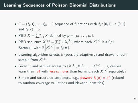
Learning Sequences of Poisson Binomial Distributions

• F = (f1, f2, . . . , fk , . . .) sequence of functions with fk : [0, 1]→ [0, 1]

and f1(x) = x .

• PBD X =∑n

i=1 Xi defined by p = (p1, . . . , pn).

• PBD sequence X (k) =∑n

i=1 X(k)i , where each X

(k)i is a 0/1

Bernoulli with E[X

]= fk(pi ).

• Learning algorithm selects k (possibly adaptively) and draws random

sample from X (k).

• Given F and sample access to (X (1),X (2), . . . ,X (k), . . .), can we

learn them all with less samples than learning each X (k) separately?

• Simple and structured sequences, e.g., powers fk(x) = xk (related

to random coverage valuations and Newton identities).

and f1(x) = x .

• PBD X =∑n

(k)i is a 0/1

Bernoulli with E[X

]= fk(pi ).

sample from X (k).

and f1(x) = x .

• PBD X =∑n

(k)i is a 0/1

Bernoulli with E[X

]= fk(pi ).

sample from X (k).

Motivation: Random Coverage Valuations

• Set U of n items.

• Family A = A1, . . . ,Am random subsets of U.

• Item i is included in Aj independently with probability pi .

• Distribution of # items included in union of k subsets,

i.e., distribution of | ∪j∈[k] Aj |

• Item i is included in the union with probability 1 − (1 − pi )k

• # items in union of k sets is distributed as n − X (k)

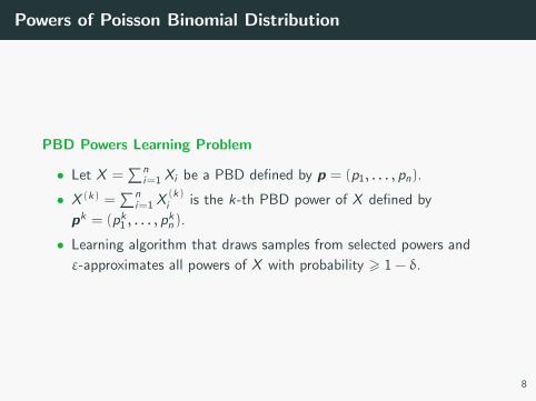
Powers of Poisson Binomial Distribution

PBD Powers Learning Problem

• Let X =∑n

i=1 Xi be a PBD defined by p = (p1, . . . , pn).

• X (k) =∑n

i=1 X(k)i is the k-th PBD power of X defined by

pk = (pk1 , . . . , pkn ).

• Learning algorithm that draws samples from selected powers and

ε-approximates all powers of X with probability > 1 − δ.

Learning the Powers of Bin(n, p)

• Estimator p =(∑N

i=1 si

)/(Nn) . If p small, e.g., p 6 1/e,

|p − p| 6 err(n, p, ε)⇒ |pk − pk | 6 err(n, pk , ε

)Intuition: error ≈ 1/

√n leaves important bits of p unaffected.

• But if p ≈ 1 − 1n ,

p = 0. 99 . . . 9︸︷︷︸log n

458382︸︷︷︸“value”

• Sampling from the first power does not reveal “right” part p, since

error ≈√

p(1 − p)/n ≈ 1/n.

• Not good enough to approximate all binomial powers (e.g.,

n = 1000, p = 0.9995, 0.99951000 ≈ 0.6064, 0.99971000 ≈ 0.7407)

• For ` = 1ln(1/p)

, p` = 1/e : sampling from `-power reveals “right” part.

i=1 si

• But if p ≈ 1 − 1n ,

p = 0. 99 . . . 9︸︷︷︸log n

458382︸︷︷︸“value”

error ≈√

p(1 − p)/n ≈ 1/n.

n = 1000, p = 0.9995, 0.99951000 ≈ 0.6064, 0.99971000 ≈ 0.7407)

• For ` = 1ln(1/p)

i=1 si

• But if p ≈ 1 − 1n ,

p = 0. 99 . . . 9︸︷︷︸log n

458382︸︷︷︸“value”

error ≈√

p(1 − p)/n ≈ 1/n.

n = 1000, p = 0.9995, 0.99951000 ≈ 0.6064, 0.99971000 ≈ 0.7407)

• For ` = 1ln(1/p)

i=1 si

• But if p ≈ 1 − 1n ,

p = 0. 99 . . . 9︸︷︷︸log n

458382︸︷︷︸“value”

error ≈√

p(1 − p)/n ≈ 1/n.

n = 1000, p = 0.9995, 0.99951000 ≈ 0.6064, 0.99971000 ≈ 0.7407)

• For ` = 1ln(1/p)

Sampling from the Right Power

Algorithm 1 Binomial Powers

1: Draw O(ln(1/δ)/ε2

)samples from Bin(n, p) to obtain p1.

2: Let ˆ← d1/ ln(1/p1)e.3: Draw O

(ln(1/δ)/ε2

)samples from B(n, p

ˆ) to get estimation q of p

4: Use estimation p = q1/ˆ

to approximate all powers of Bin(n, p).

• We assume that p 6 1 − ε2/n. If p > 1 − ε2/nd , we need

O(ln(d) ln(1/δ)/ε2

)samples to learn the right power `.

Learning the Powers vs Parameter Learning

Question: Learning PBD Powers ⇔ Estimating p = (p1, . . . , pn)?

• Lower bound of Ω(21/ε) for parameter estimation holds if we draw

samples from selected powers.

• If pi ’s are well-separated, we can learn them exactly by sampling

from powers.

Lower Bound on PBD Power Learning

• PBD defined by p with n/(ln n)4 groups of size (ln n)4 each.

Group i has pi = 1 − ai(ln n)4i , ai ∈ 1, . . . , ln n.

• Given (Y (1), . . . ,Y (k), . . .) that is ε-close to (X (1), . . . ,X (k), . . .),

we can find (e.g., by exhaustive search) (Z (1), . . . ,Z (k), . . .) where

qi = 1 − bi(ln n)4i and ε-close to (X (1), . . . ,X (k), . . .).

• For each power k = (ln n)4i−2,∣∣E[X (k)]− E

[Z (k)

]∣∣ = Θ(|ai − bi |(ln n)2) and∣∣V[X (k)

[Z (k)

]∣∣ = O((ln n)3).

• By sampling appropriate powers, we learn ai exactly:

Ω(n ln ln n/(lnn)4) samples.

[Z (k)

]∣∣ = Θ(|ai − bi |(ln n)2) and∣∣V[X (k)

[Z (k)

]∣∣ = O((ln n)3).

[Z (k)

]∣∣ = Θ(|ai − bi |(ln n)2) and∣∣V[X (k)

[Z (k)

]∣∣ = O((ln n)3).

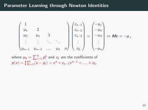
Parameter Learning through Newton Identities

µ2 µ1 3...

.... . .

µn−1 µn−2 . . . µ1 n

cn−1

cn−2

cn−3

−µ1−µ2−µ3

−µn

⇔Mc = −µ ,

where µk =∑n

i=1 pki and ck are the coefficients of

p(x) =∏n

i=1(x − pi ) = xn + cn−1xn−1 + . . .+ c0.

• Learn (approximately) µk ’s by sampling from the first n powers.

• Solve system Mc = −µ to obtain c : amplifies error by O(n3/22n

)• Use Pan’s root finding algorithm to compute |pi − pi | 6 ε : requires

accuracy 2O(−nmaxln(1/ε),ln n) in c .

• # samples = 2O(nmaxln(1/ε),ln n)

µ2 µ1 3...

.... . .

µn−1 µn−2 . . . µ1 n

cn−1

cn−2

cn−3

−µ1−µ2−µ3

−µn

⇔Mc = −µ ,

where µk =∑n

p(x) =∏n

i=1(x − pi ) = xn + cn−1xn−1 + . . .+ c0.

µ2 µ1 3...

.... . .

µn−1 µn−2 . . . µ1 n

cn−1

cn−2

cn−3

−µ1−µ2−µ3

−µn

⇔Mc = −µ ,

where µk =∑n

p(x) =∏n

i=1(x − pi ) = xn + cn−1xn−1 + . . .+ c0.

Some Open Questions

• Class of PBDs where learning powers is easy but parameter

learning is hard ?

• If all pi 6 1 − ε2

n , can we learn all powers with o(n/ε2) samples?

• If O(1) different values in p, can we learn all powers with O(1/ε2)

samples?

Graph Binomial Distributions

• Each Xi is an independent 0/1 Bernoulli trials with E[Xi ] = pi .

• Graph G (V ,E ) where vertex vi is active iff Xi = 1.

• Given G , learn distribution of # edges in subgraph induced by active

vertices, i.e., XG =∑

vi ,vj ∈E XiXj

• G clique: learn # active vertices k (# edges is k(k−1)2 ).

• G collection of disjoint stars K1,j , j = 2, . . . , Θ(√n) with pi = 1 if vi

is leaf: Ω(√n) samples are required.

Graph Binomial Distributions

• Each Xi is an independent 0/1 Bernoulli trials with E[Xi ] = pi .

• Graph G (V ,E ) where vertex vi is active iff Xi = 1.

• Given G , learn distribution of # edges in subgraph induced by active

vertices, i.e., XG =∑

vi ,vj ∈E XiXj

• G clique: learn # active vertices k (# edges is k(k−1)2 ).

• G collection of disjoint stars K1,j , j = 2, . . . , Θ(√n) with pi = 1 if vi

is leaf: Ω(√n) samples are required.

Some Observations for Single p

• If p small and G is almost regular with small degree, X is close to

Poisson distribution with λ = mp2.

• Estimating p as p =

√(∑Ni=1 si

)/(Nm) gives ε-close

approximation if G is almost regular, i.e., if∑

v deg2v = O(m2/n).

• Nevertheless, characterizing structure of XG is wide open:

Some Observations for Single p

• If p small and G is almost regular with small degree, X is close to

Poisson distribution with λ = mp2.

• Estimating p as p =

√(∑Ni=1 si

)/(Nm) gives ε-close

approximation if G is almost regular, i.e., if∑

v deg2v = O(m2/n).

• Nevertheless, characterizing structure of XG is wide open:

Thank you!

On Learning Powers of Poisson Binomial Distributions and ... · On Learning Powers of Poisson...

Documents

Transcript of On Learning Powers of Poisson Binomial Distributions and ... · On Learning Powers of Poisson...