Ion Energy Distributions in Collisionless and Collisional ...

THÈSE NO 3298 (2005)
ÉCOLE POLYTECHNIQUE FÉDÉRALE DE LAUSANNE
PRÉSENTÉE À LA FACULTÉ SCIENCES DE BASE
Institut des sciences et ingénierie chimiques
SECTION DE CHIMIE ET GÉNIE CHIMIQUE
POUR L'OBTENTION DU GRADE DE DOCTEUR ÈS SCIENCES
PAR
ingénieur physicien diplômé EPFde nationalité suisse et originaire de Sursee (LU)
acceptée sur proposition du jury:
Lausanne, EPFL2005
Richard BOSSART
Prof. Th. Rizzo, directeur de thèseProf. B. Abel, rapporteur
Dr G. Seyfang, rapporteurProf. H. van den Bergh, rapporteur
ON ISOTOPICALLY SELECTIVE COLLISIONAL ENERGY TRANSFER AND INFRARED MULTIPLE PHOTON
ABSORPTION BY VIBRATIONALLY HIGHLY EXCITED MOLECULES

Richard Bossart
On Isotopically Selective Collisional Energy Transfer and Infrared Multiple Photon
Absorption by Vibrationally Highly Excited Molecules
PhD Thesis
http://library.epfl.ch/theses/?nr=3298


Contents
Abstract IX
Version abregee XI
Kurzfassung XIII
1 Introduction 3
1.1 A new laser isotope separation scheme called OP-IRMPD . . . . . . . . . 4
1.2 Aim of this work . . . . . . . . . . . . . . . . . . . . . . . . . . . . . . . 8
1.3 Structure of this work . . . . . . . . . . . . . . . . . . . . . . . . . . . . 12
Bibliography . . . . . . . . . . . . . . . . . . . . . . . . . . . . . . . . . . . . 13
2 Background information 19
2.1 Spectroscopy and intramolecular dynamics of CF3H . . . . . . . . . . . . 19
2.2 IR multiple photon dissociation (IRMPD) . . . . . . . . . . . . . . . . . 41
2.3 Collisional vibrational relaxation . . . . . . . . . . . . . . . . . . . . . . 52
Bibliography . . . . . . . . . . . . . . . . . . . . . . . . . . . . . . . . . . . . 72
3 Experimental setup 87
3.1 Optical setup of our experiments . . . . . . . . . . . . . . . . . . . . . . 87
3.2 Working pressure . . . . . . . . . . . . . . . . . . . . . . . . . . . . . . . 96
3.3 Synthesis of 13CF3H . . . . . . . . . . . . . . . . . . . . . . . . . . . . . 99
Bibliography . . . . . . . . . . . . . . . . . . . . . . . . . . . . . . . . . . . . 104
4 Experimental investigations 105
4.1 Introduction . . . . . . . . . . . . . . . . . . . . . . . . . . . . . . . . . . 105
V
VI CONTENTS
4.2 State specificity of the increase of isotopic selectivity upon leaving a time-
delay between the pre-excitation and the dissociation lasers . . . . . . . . 110
4.3 Properties of collision-free IRMPD of excited molecules: photofragment
excitation spectrum and dissociation selectivity of vibrationally excited
CF3H . . . . . . . . . . . . . . . . . . . . . . . . . . . . . . . . . . . . . 114
4.4 Separation of different mechanisms changing the wavelength of the dis-
sociation laser . . . . . . . . . . . . . . . . . . . . . . . . . . . . . . . . . 127
4.5 Separation of different mechanisms using a carbon-13 enriched sample . . 133
4.6 Discussion and conclusion . . . . . . . . . . . . . . . . . . . . . . . . . . 148
Bibliography . . . . . . . . . . . . . . . . . . . . . . . . . . . . . . . . . . . . 151
5 Numerical simulations of V-V energy transfer and IRMPD of CF3H 153
5.1 Absorption and emission spectra of an excited molecule . . . . . . . . . . 154
5.2 Numerical simulations of vibrational energy transfer between excited and
ground state molecules . . . . . . . . . . . . . . . . . . . . . . . . . . . . 165
5.3 Numerical simulations of IRMPD in the presence of collisions . . . . . . . 187
Bibliography . . . . . . . . . . . . . . . . . . . . . . . . . . . . . . . . . . . . 222
6 Conclusions and Outlook 229
6.1 Isotopically selective collisional vibrational relaxation . . . . . . . . . . . 229
6.2 Enhancement of isotopic selectivity in our MLIS process . . . . . . . . . 231
Bibliography . . . . . . . . . . . . . . . . . . . . . . . . . . . . . . . . . . . . 232
APPENDICES 233
A Development of formulae for pumping molecules through a low density
regime (“case C”) 235
A.1 Qualitative explanations . . . . . . . . . . . . . . . . . . . . . . . . . . . 236
A.2 Calculations details . . . . . . . . . . . . . . . . . . . . . . . . . . . . . . 238
A.3 Attempts to generalise case C calculations . . . . . . . . . . . . . . . . . 240
Bibliography . . . . . . . . . . . . . . . . . . . . . . . . . . . . . . . . . . . . 242
B Collisional quenching of LIF 243
Bibliography . . . . . . . . . . . . . . . . . . . . . . . . . . . . . . . . . . . . 245
CONTENTS VII
C CO2 laser fluence control and measurement 247
C.1 Attenuation of the CO2 laser beam . . . . . . . . . . . . . . . . . . . . . 247
C.2 Calculation of the fluence . . . . . . . . . . . . . . . . . . . . . . . . . . 248
D CO2 laser fluence dependence of the decay rate 253
E The numerical codes for the calculation of IRMPD in the presence of
collisions 257
E.1 Generalities . . . . . . . . . . . . . . . . . . . . . . . . . . . . . . . . . . 257
E.2 The code . . . . . . . . . . . . . . . . . . . . . . . . . . . . . . . . . . . . 258
Notations and abbreviations 271
List of tables 280
List of figures 283
Acknowledgements 289
Curriculum vitae 291

VIII CONTENTS

Abstract
This study focuses on an interesting and important phenomenon that was employed in
a new approach to laser isotope separation that has been recently proposed and devel-
oped in our laboratory for highly selective separation of carbon isotopes. This approach
consists of pre-exciting CF3H molecules with the desired isotope to a low vibrational
overtone of the CH-stretch with a subsequent selective infrared multiple photon disso-
ciation (IRMPD) of only the pre-excited molecules by a CO2-laser pulse. Significant
isotopic shifts of the employed CH overtone bands already allow high selectivity at the
pre-excitation step. This selectivity, however, can be further greatly increased by in-
creasing the pressure of the sample gas and/or the delay between the two laser pulses;
that is, by increasing the number of molecular collisions during the process. At first
glance, the observed effect contradicts the general expectations that the isotopic selec-
tivity of such a process should drop with an increase in the number of collisions because
of vibrational energy transfer between different isotopic species. In this work we have
studied this phenomenon and found its physical origins.
We propose the contribution of two different mechanisms to the observed enhance-
ment of isotopic selectivity by collisions. First, the vibrational collisional relaxation
itself is isotopically selective, that is vibrationally excited 12CF3H relax on the bath
of cold, 12CF3H, molecules faster than the excited 13CF3H do on the same bath. The
primary reason for such a selectivity could be a significant isotopic shift of the vibration
(CF-stretch, we believe) that mediates the energy transfer.
A second mechanism arises from the difference between the IRMPD probabilities of the
two isotopic species by the CO2 laser tuned to a particular wavelength that enhances
the dissociation yield of the targeted, carbon-13, species. As collisional deactivation of
IX
X ABSTRACT
both species increases the number of photons they have to absorb to be dissociated, this
difference in dissociation probability increases as well, yielding an additional isotopic
selectivity of the process.
We perform a set of experiments and numerical simulations to investigate these two
mechanisms. Experimentally we find that, indeed, collisional vibrational deactivation
of CF3H is isotopically selective. This is, perhaps, the first direct observation of iso-
topically selective collisional relaxation of highly excited medium-sized molecules. At
low pressures and increased time-delay between the lasers both suggested mechanisms
contribute equally to the enhancement of isotopic selectivity (with a slight dominance of
the IRMPD step). We also perform numerical simulations of vibrational energy transfer
(VET) between highly excited and cold CF3H of both isotopic species. The model we
employ includes V-V energy transfer due to long-range dipole-dipole interactions and
V-V’,T,R energy transfer due to head-on collisions between two molecules. The results
reproduce well the measured isotopic selectivity in vibrational energy transfer. At the
next step, we propose a model for the simulation of the laser isotope separation process.
We solve the master equations including vibrational energy transfer and absorption and
stimulated emission of IR photons. The main improvement of our calculations with re-
spect to existing models is that we introduce a dependence of the absorption/emission
rates on the frequency of the laser, the internal energy of the molecule and its iso-
topic species. We are able to reproduce our experiments numerically and thus gain
information on the laser isotope separation process. In particular, we find that at high
sample pressures the mechanism of isotopically selective IRMPD rates prevails over the
mechanism of different collisional relaxation rates.

Version abregee
Notre etude se concentre sur un phenomene interessant et important qui a ete utilise
dans une nouvelle approche de separation isotopique par laser qui a ete proposee et
developpee dans notre laboratoire pour la separation hautement selective de carbone-
13. Cette approche consiste a exciter des molecules de CF3H avec l’isotope desire via
un overtone de la vibration CH suivi d’une dissociation selective des molecules excitees
par absorption multiple de photons infrarouges (IRMPD, “Infrared multiple photon dis-
sociation”) provenant d’un laser CO2. Une grande selectivite est obtenue a l’excitation
initiale qui est due a un deplacement isotopique important de l’overtone de la vibration
CH. Cette selectivite peut etre largement augmentee en augmentant la pression du gaz
et/ou la duree entre les deux impulsions laser utilisees, ce qui augmente le nombre de
collisions moleculaires pendant le processus. A premiere vue, cet effet est en contra-
diction avec la diminution attendue de la selectivite isotopique lorsque le nombre de
collisions augmente, a cause du transfert d’energie vibrationnelle entre les differentes
especes isotopiques. Dans ce travail, nous avons etudie cet effet et trouve ses origines
physiques.
Nous proposons la contribution de deux mecanismes differents a l’augmentation de la
selectivite due aux collisions. Premierement, la relaxation vibrationnelle par collisions
est isotopiquement selective en elle-meme, c’est-a-dire que des molecules 12CF3H ex-
citees se desactivent sur les molecules 12CF3H non excitees environnantes plus vite que
des molecules 13CF3H excitees. La raison principale de cette selectivite pourrait etre
un deplacement isotopique important de la vibration qui est a l’origine de ce transfert
d’energie (probablement la vibration CF).
Un deuxieme mecanisme est du a une difference de l’efficacite de l’IRMPD des deux
XI
XII VERSION ABREGEE
especes isotopiques par le laser CO2 fixe a une longueur d’onde particuliere qui aug-
mente le rendement de dissociation du 13CF3H. Puisque la relaxation par collisions des
deux especes isotopiques augmente le nombre de photons qu’elles doivent absorber pour
etre dissociees, cette difference de probabilite de dissociation est aussi augmentee, ce
qui mene a une plus grande selectivite isotopique du processus.
Nous conduisons des experiences et des simulations numeriques afin d’etudier ces deux
mecanismes. Experimentalement, nous observons que la relaxation vibrationnelle par
collisions de CF3H est isotopiquement selective. Ceci est, peut-etre, la premiere ob-
servation directe de relaxation par collisions isotopiquement selective de molecules de
taille moyenne hautement excitees. A basses pressions et avec un plus grand inter-
valle de temps entre les lasers les deux mecanismes contribuent de maniere egale a
l’augmentation de la selectivite isotopique (avec une legere dominance de l’IRMPD se-
lective). Nous effectuons des simulations numeriques du processus de transfert d’energie
vibrationnelle (VET, “vibrational energy transfer”) entre des molecules CF3H des deux
especes isotopiques hautement excitees et non excitees. Le modele utilise comprend le
transfert d’energie V-V du a l’interaction dipole-dipole a longue distance et le transfert
d’energie V-V’,T,R du a des collisions frontales entre deux molecules. Les resultats re-
produisent bien la selectivite du transfert d’energie vibrationnelle mesuree experimenta-
lement. Dans une deuxieme etape, nous proposons un modele pour la simulation du pro-
cessus de separation isotopique par laser. Nous resolvons les equations maıtresses inclu-
ant la relaxation vibrationnelle, ainsi que l’absorption et l’emission stimulee de photons
infrarouges. L’amelioration principale de notre approche par rapport aux modeles exis-
tants est l’introduction d’une dependance des vitesses d’absorption et d’emission en fonc-
tion de la frequence du laser, de l’energie interne et de l’espece isotopique de la molecule.
Nous sommes en mesure de reproduire nos experiences de maniere numerique et ainsi
d’obtenir des informations sur le processus de separation isotopique par laser. Nous
constatons notamment qu’a hautes pressions, le mecanisme de la difference d’efficacite
de l’IRMPD prevaut sur celui de la desactivation par collisions isotopiquement selective.
Kurzfassung
Diese Untersuchung ist einem interessanten und wichtigen Phanomen gewidmet, welches
in einer neuen Methode zu einer hochselektiven Isotopentrennung mit Lasern ausgenutzt
wird, das wir in unserem Laboratorium entwickelt haben. Der Ansatz dazu ist, CF3H
Molekule mit dem gewunschten Isotop via einen Oberton der CH Schwingung anzure-
gen, um sie anschliessend mit Absorption mehrerer Infrarot-Photonen die angeregten
Molekule selektiv zu disoziieren (IRMPD, “Infrared multiple photon dissociation”).
Grosse isotopische Verschiebungen der CH Schwingung erlauben bereits eine hohe Se-
lektivitat. Diese Selektivitat kann sehr gesteigert werden, indem der Probendruck oder
die Verzogerung zwischen den Laser-Pulsen erhoht wird. Dadurch wird die Anzahl
molekularer Stosse erhoht. Diese Beobachtung steht im Widerspruch zu der allge-
meinen Erwartung, dass die isotopische Selektivitat in einem solchen Prozess wegen der
vibrationeller Energieubertragung fallen sollte. In dieser Arbeit studierten wir dieses
Phanomen und haben dessen physikalischen Ursprunge entdeckt.
Wir schlagen den Beitrag zweier verschiedener Mechanismen fur den beobachteten
Anstieg der isotopischer Selektivitat wegen der Stossen vor. Erstens, die vibrationelle
Energieubertragung in den Stossen ist isotopisch selektiv, d.h. die angeregten 12CF3H
Molekule verlieren ihre Energie schneller als angeregte 13CF3H Molekule in den Stossen
mit kalten 12CF3H Molekulen. Der Grund fur diese Selektivitat ist die isotopische Ver-
schiebung der CF Schwingung, welche fur die Energieubertragung verantwortlich ist.
Ein zweiter Mechanismus grundet auf den verschiedenen Geschwindigkeiten, mit welchen
die Molekule die Infrarot-Photonen absorbieren. Die Energie dieser Photonen ist der-
massen optimiert, dass sie mit den Kohlenstoff-13 haltigen Molekulen moglichst in Res-
onanz sind. Da die Anzahl der zu absorbierenden Photonen wegen der Stosse erhoht
XIII
XIV KURZFASSUNG
wird, wird dadurch der Unterschied in der Dissoziationswahrscheinlichkeit zusatzlich
erhoht, was zu einer gesteigerten isotopischen Selektivitat fuhrt.
Wir fuhren mehrere Experimente und numerische Simulationen durch, um die zwei
Mechanismen zu untersuchen. Experimentell erkennen wir, dass die Energieubertragung
in Stossen in der Tat isotopisch selektiv ist. Dies ist wahrscheinlich die erste direkte
Beobachtung von isotopisch selektiver Energieubertragung in Stossen von hochang-
eregten, mittelgrossen Molekulen. Bei tiefen Probendrucken und erhohter Verzogerung
ist der Beitrag der beiden Mechanismen zu der Erhohung der isotopischen Selektivitat
ungefahr gleich gross (mit einer leichten Dominanz der verschiedenen IRMPD Dissozi-
ationsgeschwindigkeiten). Wir haben auch Simulationen zu der Ubertragung von vi-
brationeller Energie in Stossen (VET, “vibrational energy transfer”) zwischen hochang-
eregten und kalten CF3H verschiedener isotopischen Spezies durchgefuhrt. Das Modell
baut einerseits auf vibrationeller V-V Energieubertragung uber grosse Distanzen auf,
welche auf der Dipol-Dipol-Wechselwirkung beruht, andrerseits auf Wechselwirkungen
uber kurze Distanzen, die zu V-V’,T,R Energieubertragung fuhren. Die Resultate geben
die experimentell beobachteten isotopische Selektivitat uberzeugend wieder. In einem
zweiten Schritt schlagen wir ein Modell fur die Simulation unseres Systems zur Iso-
topentrennung mit Lasern vor. Wir haben die Hauptgleichungen gelost, die sowohl die
vibrationelle Energieubertragung in Stossen als auch die Absorption und die stimulierte
Emission von IR-photonen beinhaltet. Die wichtigste Verbesserung unserer Simulatio-
nen gegenuber existierenden Modellen besteht darin, dass wir fur die Absorptions- und
Emissionswahrscheinlichkeiten eine Abhangigkeit von der Wellenlange des Lasers, der vi-
brationellen Energie des Molekuls und der isotopischen Zusammensetzung des Molekuls
berucksichtigen. Wir konnen so unsere experimentelle Beobachtungen numerisch repro-
duzieren und auf diese Weise Informationen uber den Prozess der Isotopentrennung mit
Lasern gewinnen. Insbesondere finden wir, dass bei erhohten Probendrucken der Mech-
anismus der verschiedenen IRMPD Wahrscheinlichkeiten wichtiger ist als der Mecha-
nismus von isotopischer selektiver Energieubertragung.

THE THESIS


Chapter 1
Introduction
Isotopes are atoms of a chemical element whose nuclei have the same atomic number
(number of protons) but different atomic weights (i.e. different number of neutrons).
The word “isotope”, meaning at the same (Greek, “iso”) place (Greek, “topos”), comes
from the fact that isotopes are located at the same place on the periodic table1, 2. The
first isotopes were discovered experimentally in the early 1930’s3.
Numerous applications in different areas require isotopically pure materials. For ex-
ample, a recent medical test called “Urea breath test” (UBT4–6) has been developed in
order to detect a peptic ulcer disease caused by a helicobacter pylori7, 8 infection in the
body. For this, the patient swallows a capsule containing carbon-13 enriched (NH2)2CO
(urea). In the presence of the helicobacter pylori this molecule is broken down; one
of the products is CO2 which is later exhaled by the patient. The infection can be
diagnosed by measuring the isotopic ratio of the carbon species in the exhaled CO2; in
this case an excess of carbon-13 can be observed.
The production of isotopically pure material is done by gas centrifuge, gaseous dif-
fusion, chemical exchange, electro-magnetic separation or low temperature distillation9.
An alternative lies in laser isotope separation (LIS10–13) which is based on spectroscopic
differences between different isotopic species. Here, one distinguishes between atomic
vapour laser isotope separation (AVLIS), where atoms are directly ionised, molecular
laser isotope separation (MLIS), where molecules are dissociated via infrared multiple
photon excitation (IRMPE) and chemical reaction by isotope selective laser activation
3
4 CHAPTER 1. INTRODUCTION
(CRISLA) in which case the excited molecules react chemically.
1.1 A new laser isotope separation scheme called OP-IRMPD
Traditional approaches to MLIS consist of irradiating a sample gas with a laser in the
10µm wavelength region, typically by CO2 or NH3 lasers, in order to selectively disso-
ciate the molecules with the desired isotope.
Recently, an original approach to molecular laser isotope separation was proposed in our
laboratory14–21. A key point of this new approach is the ability of IRMPD to perform a
selective dissociation of vibrationally pre-excited molecules without significant dissocia-
tion of the ground state species under some specific circumstances. This specific feature
of IRMPD was first demonstrated for hydrated hydronium cluster ions22 H3O+ · (H2O)n
(n=1, 2, 3), and later it was used in a successful development of a spectroscopic tech-
nique for detecting weak vibrational overtone transitions23. The same feature, combined
with isotopically selective vibrational overtone pre-excitation and collisional enhance-
ment of isotopic selectivity, comprises the new approach for isotope separation. We first
describe this spectroscopic technique called “IRLAPS” which led to the invention of
the new approach to molecular laser isotope separation, then we will give some details
about the MLIS technique itself.
1.1.1 IRLAPS detection scheme
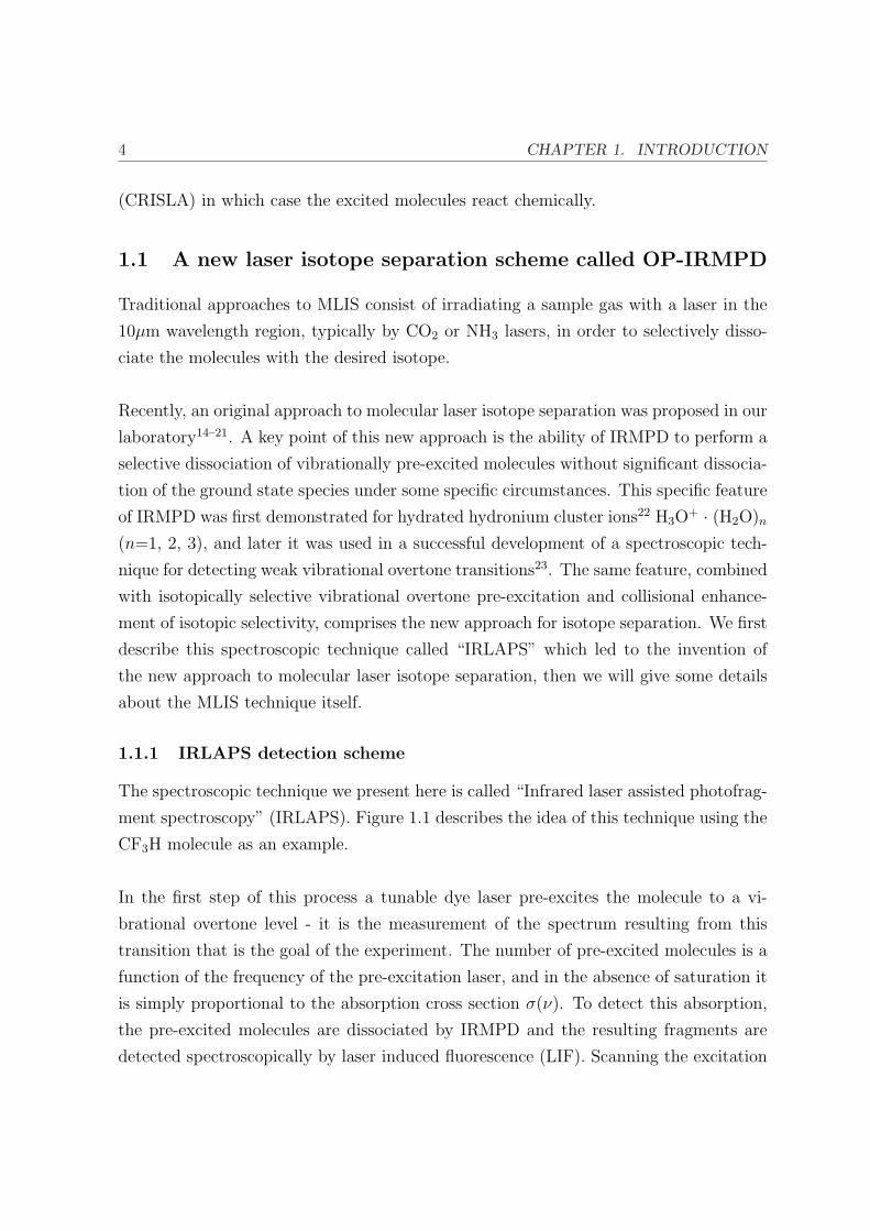
The spectroscopic technique we present here is called “Infrared laser assisted photofrag-
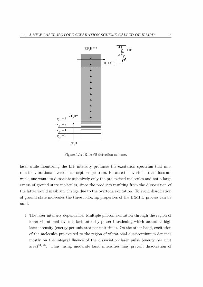
ment spectroscopy” (IRLAPS). Figure 1.1 describes the idea of this technique using the
CF3H molecule as an example.
In the first step of this process a tunable dye laser pre-excites the molecule to a vi-
brational overtone level - it is the measurement of the spectrum resulting from this
transition that is the goal of the experiment. The number of pre-excited molecules is a
function of the frequency of the pre-excitation laser, and in the absence of saturation it
is simply proportional to the absorption cross section σ(ν). To detect this absorption,
the pre-excited molecules are dissociated by IRMPD and the resulting fragments are
detected spectroscopically by laser induced fluorescence (LIF). Scanning the excitation
1.1. A NEW LASER ISOTOPE SEPARATION SCHEME CALLED OP-IRMPD 5
Figure 1.1: IRLAPS detection scheme.
laser while monitoring the LIF intensity produces the excitation spectrum that mir-
rors the vibrational overtone absorption spectrum. Because the overtone transitions are
weak, one wants to dissociate selectively only the pre-excited molecules and not a large
excess of ground state molecules, since the products resulting from the dissociation of
the latter would mask any change due to the overtone excitation. To avoid dissociation
of ground state molecules the three following properties of the IRMPD process can be
used.
1. The laser intensity dependence. Multiple photon excitation through the region of
lower vibrational levels is facilitated by power broadening which occurs at high
laser intensity (energy per unit area per unit time). On the other hand, excitation
of the molecules pre-excited to the region of vibrational quasicontinuum depends
mostly on the integral fluence of the dissociation laser pulse (energy per unit
area)24, 25. Thus, using moderate laser intensities may prevent dissociation of
6 CHAPTER 1. INTRODUCTION
the ground-state molecules, whereas pre-excited molecules still may be efficiently
dissociated provided the fluence of the dissociation laser is sufficient.
2. Anharmonic red-shift of the absorption spectrum of excited molecules23, 26. Be-
cause of this red-shift, applying a dissociation laser wavelength detuned to the red
side from the maximum of the absorption spectrum of ground-state molecules will
result in preferential multiple photon excitation of pre-excited molecules.
3. Fluence dependence. The initial energy level of the multiple photon excitation pro-
cess for pre-excited molecules lies higher than the one for ground state molecules.
It means that pre-excited molecules need to collect less infrared photons from the
dissociation laser to reach its dissociation threshold. Thus, the laser fluence re-
quired for dissociation of pre-excited molecules is lower26, 27. The correct choice of
the dissociation laser fluence may further increase the discrimination between the
ground-state and pre-excited molecules.
The advantage of the IRLAPS method as a spectroscopic technique is its high sensitivity
which allows the detection of extremely weak vibrational overtone transitions under
molecular jet expansion conditions. Since its development in the beginning of 1990’s,
the IRLAPS method has been applied for obtaining high resolution overtone spectra of
a number of molecules, contributing to understanding the dynamics of intramolecular
vibrational energy redistribution (IVR) process23, 28–34.
1.1.2 OP-IRMPD system for isotope separation
Two findings in the experiments, where IRLAPS was applied for the detection of highly
excited molecules, have lead to the development of our isotope separation process:
1. Excitation of high vibrational overtones can be isotopically selective.
2. The dissociation of molecules in the ground state can be suppressed in an effective
way by appropriately adjusting the fluence and the wavelength of the dissociation
laser.
The new approach consists of two major steps: in the first step, a near-infrared laser
pulse pre-excites molecules containing the desired isotope via a low vibrational over-
tone transition of a high frequency vibrational mode. In the second step, a CO2 laser
1.1. A NEW LASER ISOTOPE SEPARATION SCHEME CALLED OP-IRMPD 7
pulse selectively dissociates the pre-excited molecules. Finally, the dissociation prod-
ucts enriched in the desired isotope are chemically converted to a stable molecule (CF2+
CF2→ C2F4) that is different from the parent molecule and physically separated from
the latter, for instance, by distillation. This method is called “Overtone Pre-excitation -
Infrared Multiple Photon Dissociation” (OP-IRMPD). In this scheme, the isotopic com-
position of the products is mainly determined by the selectivity of the pre-excitation
step. Although the pre-excitation laser is tuned in such a way that a maximum amount
of 13CF3H molecules is pre-excited, some of the 12CF3H molecules are pre-excited as
well, because a P-branch of the absorption feature for 12CF3H overlaps with the Q-
branch of the absorption feature for 13CF3H.
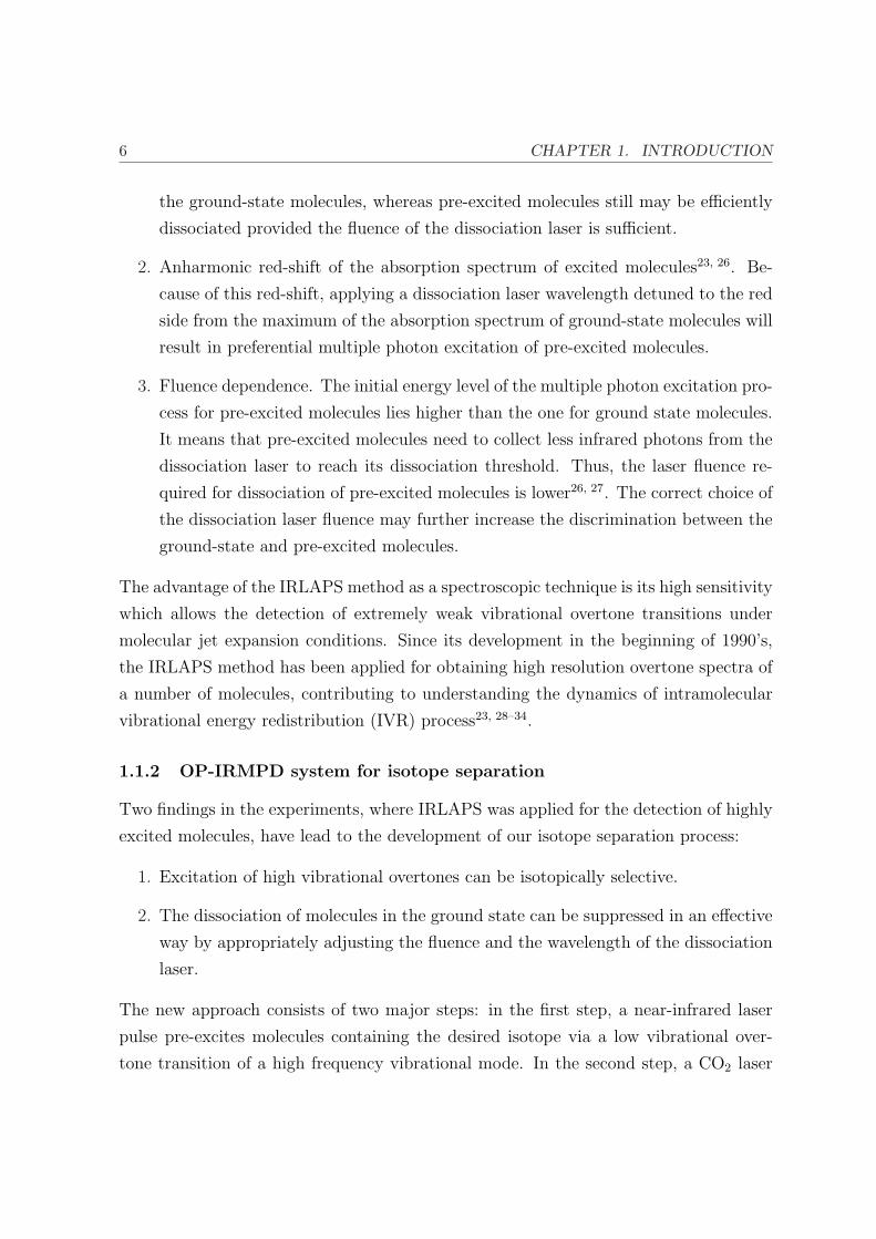
We show in figure 1.2 an IRLAPS action spectrum of CF3H around 8800 cm−1 which
is obtained by measuring the total amount of LIF as a function of the pre-excitation
energy. The small feature at ∼8753 cm−1 is due to the carbon-13 isotopomer of CF3H.
In our MLIS scheme we excite the molecules at this wavelength.
LIF
sig
nal [
a.u.
]
8800878087608740
Frequency [cm-1
]
87568754875287508748
Frequency [cm-1
]
31 band12
CF3H
31 band13
CF3H
Figure 1.2: Spectrum of the 31 transition in CF3H. The large peak at ∼8793 cm−1 is assigned
to the 12CF3H isotopomer, the small peak at∼8753 cm−1 is assigned to the 13CF3H
isotopomer. The sample is in its natural isotopic abundance.
8 CHAPTER 1. INTRODUCTION
1.2 Aim of this work
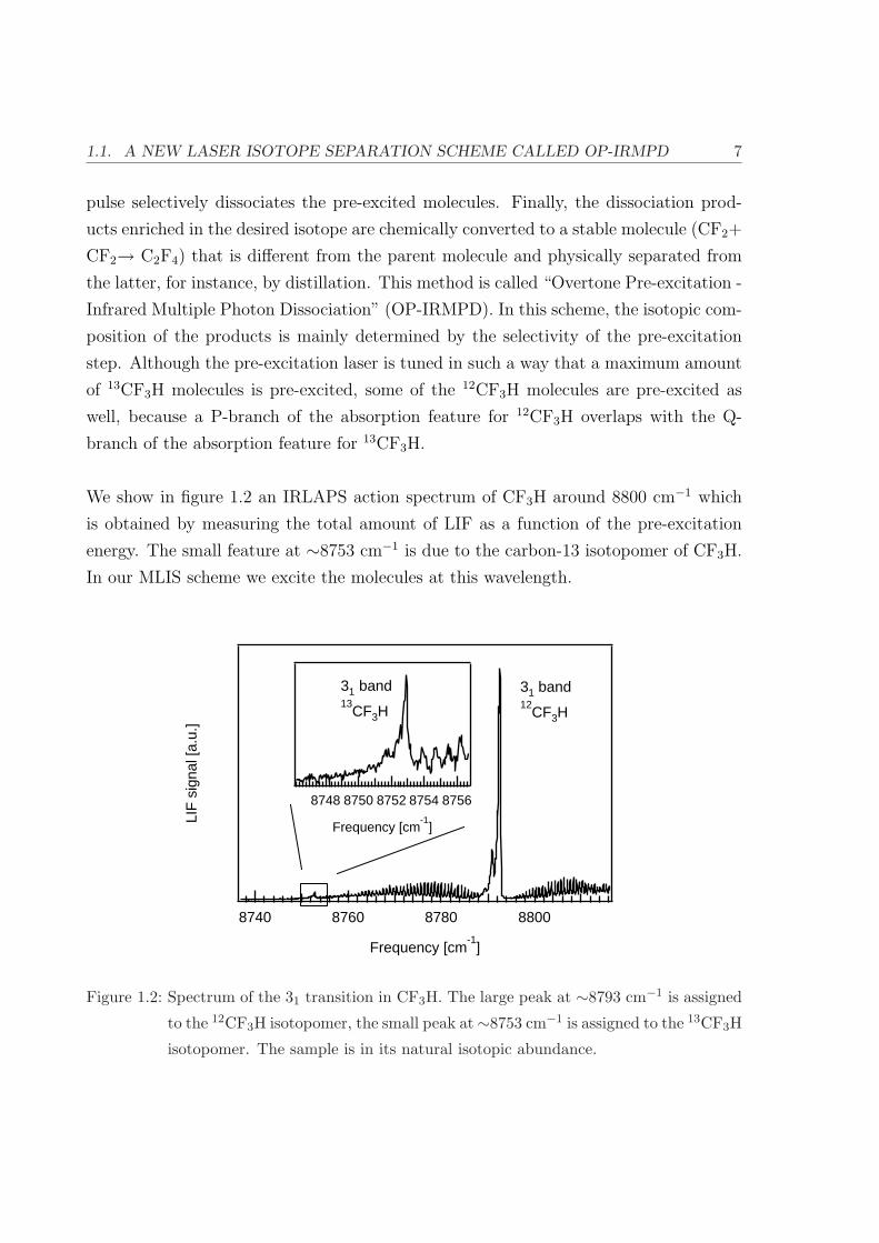
Experimentally it has been observed, that the isotopic abundance in the products de-
pends on the sample pressure and on the delay between the two lasers used in this
scheme15, 16. Figure 1.3 shows the observed effect.
Nor
mal
ized
pro
duct
ivity
, p12
, p13
3002001000
Delay, ns
0.98
0.96
0.94
0.92
0.90
Abundance, α
12C
13C
(a) Isotopic selectivity and productivity as a
function of the time-delay between the two
lasers.
1.0
0.8
0.6
0.4
0.2
0.0Pro
duct
ivity
, p13
, arb
. u.
50403020100
Pressure, mBar
0.96
0.92
0.88
0.84
Abundance, α
(b) Isotopic selectivity and productivity of 13C
containing products as a function of the sample
pressure.
Figure 1.3: Observed effect we study in this thesis. It shows the • isotopic enrichment of the
products (right axes) and the productivity of N 12C and ¥ 13C containing products
(left axes). The isotopic selectivity increases as the delay between the two lasers
(left) or the sample pressure (right) is increased. Data from Boyarkin16.
The experimental observations shown in figure 1.3 have been explained by an effect of
collisional relaxation occurring between the pre-excited molecules and the surrounding
molecules. At first glance, this increase of selectivity contradicts normal expectations.
Indeed, collisional vibrational energy transfer between the two different isotopic species
should scramble initial isotopic selectivity gained in the pre-excitation step. Many pre-
vious works with other MLIS schemes have been performed at low pressures in order not
to scramble isotopic selectivity of the process35–40. Some authors have reported a slight
increase of isotopic selectivity in IRMPD experiments upon an increase of the sample
pressure41, 42 or the time-delay between two IR lasers43, 44. Although not complete, some
tentative explanations have been delivered. For example, competition between IRMPD
1.2. AIM OF THIS WORK 9
and collisional relaxation42 or isotopically selective collisional relaxation44 have been
proposed.
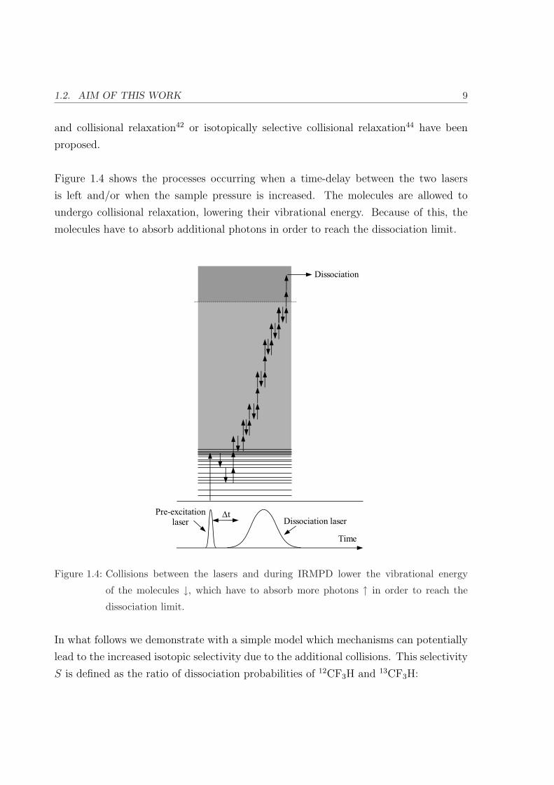
Figure 1.4 shows the processes occurring when a time-delay between the two lasers
is left and/or when the sample pressure is increased. The molecules are allowed to
undergo collisional relaxation, lowering their vibrational energy. Because of this, the
molecules have to absorb additional photons in order to reach the dissociation limit.
Figure 1.4: Collisions between the lasers and during IRMPD lower the vibrational energy
of the molecules ↓, which have to absorb more photons ↑ in order to reach the
dissociation limit.
In what follows we demonstrate with a simple model which mechanisms can potentially
lead to the increased isotopic selectivity due to the additional collisions. This selectivity
S is defined as the ratio of dissociation probabilities of 12CF3H and 13CF3H:
10 CHAPTER 1. INTRODUCTION
S :=13D12D
(1.1)
and the enhancement of isotopic selectivity is defined by
E :=S
S0
=13D/12D
13D0/12D0
, (1.2)
where the dissociation probabilities xD at a higher sample pressure or a large time-delay
between the lasers are compared to a the dissociation probabilities xD0 at a zero time-
delay between the lasers and a low sample pressure.
For the purpose of the demonstration below we will assume the up-pumping rates of
the molecules κu due to the dissociation laser radiation such as the collisional relaxation
rates κd independent on the vibrational energy of the molecule, which is not strictly
true, but demonstrates the underlying physical ideas. If a pre-excited xCF3H molecule
(x=12, 13) has a dissociation probability xD0 at a zero time-delay between the lasers and
at low pressures, then the dissociation probability xD in a situation given in figure 1.4
is given by
xD ≈ xD0 · xσxN , (1.3)
where σ ≈ κu · Φ < 1 is the probability of the molecule absorbing a photon of the laser
radiation field, Φ is the fluence of the dissociation laser pulse and N is the number of
additional photons to be absorbed in order to compensate for the loss of vibrational
energy in collisions. The enhancement E of the isotopic selectivity S of the process is
hence given by
E = SS0
=13D12D
/13D012D0
=(13κu·Φ)
13N
(12κu·Φ)12N
.
(1.4)
The enhancement of isotopic selectivity E can be different from 1 in two cases: both
in the case that the up-pumping rates via IRMPD are different (12κu 6= 13κu) and in
the case of different numbers of additional photons to be absorbed (12N 6= 13N). This
number of additional photons is proportional to the collisional relaxation rate:
1.2. AIM OF THIS WORK 11
xN ≈ xκd · p · (∆t + τd) , (1.5)
where xκd is the relaxation rate, p the sample pressure, ∆t the time-delay between the
two lasers and τd the typical time for a molecule to be dissociated‡.
We hence propose two mechanisms which can lead to the enhancement of isotopic se-
lectivity:
12κu 6= 13κu Different IRMPD rates12κd 6= 13κd Different vibrational relaxation rates
Using these two ideas, “Isotopically selective IRMPD rates” and “Isotopi-
cally selective vibrational relaxation rates”, the goal of this thesis is to
quantify the relative influences of the two mechanisms to the enhancement
of isotopic selectivity upon an increase of either the time-delay between the
laser pulses or the sample pressure.
For this, fundamental properties such as the interaction between molecules and laser
radiation (infrared multiple photon dissociation - IRMPD) and vibrational energy trans-
fer (VET) between two colliding molecules are studied. By means of this fundamental
research we both gain understanding of the phenomena under investigation and under-
stand the OP-IRMPD process better.
In addition to this, we will be interested in knowing to what extent any differences
in vibrational relaxation rates and/or up-pumping through IRMPD is a general feature
of vibrationally excited CF3H, or whether this is accidentally caused through different
couplings of the excited vibrational states in 12CF3H and 13CF3H to the other vibrational
modes of the molecule. It is known that the state to which the molecules are initially
excited are mixed with other (unidentified) close lying states, and that the couplings are
not equally strong30. It is possible, that because of this the overall energy redistribu-
tion in the molecule takes place on different time-scales for the two isotopomers which
hinders or enhances the first steps of collisional relaxation or IRMPD. Can we treat the
vibrational energy of a molecule in a statistical manner (i.e. the energy is completely
‡τd depends on the isotopic species, but for simplicity we set them equal. This does not change the reasonings.
12 CHAPTER 1. INTRODUCTION
randomised over the molecule) or do we have to take into account the exact state the
molecules are prepared in ?
In order to investigate on the contributions of the two mechanisms to the increase
of isotopic selectivity, the work is performed as follows:
• For time-delayed lasers at a low sample pressure: the determination is done ex-
perimentally, as the two mechanisms occur temporally separated allowing a clear
discrimination of the two mechanisms.
• For an increased sample pressure: the determination is done in numerical simula-
tions, as an experimental approach is more difficult to realise.
1.3 Structure of this work
This work is divided into five chapters.
• In this chapter we have stated the problem we wish to study.
• For the convenience of the reader, chapter 2 gives some background information
relevant to the subject of our study. It consists of three sections: the first one
describes the spectroscopy and intramolecular dynamics of CF3H, the second one
describes theoretical approaches for a treatment of IR multiple photon dissociation
(IRMPD), and in the third section we give an overview of the field of collisional
energy transfer (CET).
• In the third chapter we propose detailed descriptions of our experimental setup.
• In chapter 4 we give an overview of different experiments we perform in order to
investigate the phenomenon described above. This is organised as follows: after
a brief introduction, a first small section describe some experiments performed
in order to address the question of accidental resonances between the 31 and an
other (unidentified) one. Then, we describe experiments performed under collision-
free conditions, where any dissociation selectivity is obtained because of different
IRMPD efficiencies. Then we propose two sets of experiments where we try to
separate the different mechanisms leading to an increased isotopic selectivity: first,

BIBLIOGRAPHY 13
we change the wavelength of the dissociation laser radiation and then we work
with isotopically enriched CF3H. The chapter is concluded by a discussion of the
experimental results.
• Chapter 5 is dedicated to numerical simulations. There are essentially two impor-
tant sections: simulations of vibrational energy transfer, and simulations of the
overall processes in our MLIS process. A separate chapter treats the absorption
and emission spectrum of vibrationally excited CF3H.
• Finally, we conclude with the take home message of this work.
Bibliography
[1] F. Soddy. Infra-atomic charge. Nature, 92:399–400, 1913.
[2] F. Soddy. The radio-elements and the periodic law. Chemical News, 107:97–99,
1913.
[3] Harold C. Urey, F. G. Brickwedde, and G. M. Murphy. A Hydrogen Isotope of
Mass 2 . Phys. Rev., 39:164–165, 1932.
[4] Barry J. Marshall. Methods for the diagnosis of gastrointestinal disorders . US
Patent Number 4,830,010 (May 16, 1989).
[5] S. Koletzko, M. Haisch, I. Seeboth, B. Braden, K. Hengels, B. Koletzko, and
P. Hering. Isotope selective nondispersive infrared spectrometry for detection of
helicobacter-pylori infection with C-13-Urea Breath Test . Lancet, 345(8955):961–
962, 1995.
[6] Graham, Malaty, Cole, Martin, and Klein. Simplified 13C-Urea Breath Test for
Detection of Helicobacter pylori Infection . The American Journal of Gastroen-
terology, 96:1741–1745, 2001.
[7] Author unknown. ‘Guinea pig’ doctor uncovers new cause of ulcers - and the cure
. The Star, A copy can be obtained upon request from the author of this thesis.,
1984.

14 CHAPTER 1. INTRODUCTION
[8] Harry L.T. Mobley, George L. Mendz, and Stuart L. Hazell, editors. Helicobacter
pylori : physiology and genetics. Washington, D.C. : ASM Press, 2001.
[9] J.-M. Cavedon. La separation isotopique . Ann. Phys. Fr., 25(2):327–341, 2000.
[10] V. S. Letokhov. Use of lasers to control selctive chemical reactions. Science,
180:451–458, 1973.
[11] V. S. Letokhov. Laser isotope separation. Nature, 277:605–610, 1979.
[12] V. S. Letokhov. Laser-induced processes in spectroscopy, isotope separation, and
photochemistry. Sov. Phys. Uspekhi, 29:70–81, 1986.
[13] V. Y. Baranov, editor. Isotopes: properties, production, applications. IzdAT,
Moscow, 2000 (in Russian).
[14] Thomas R. Rizzo and Oleg V. Boiarkine. Laser Isotope Separation Method Em-
ploying Isotopically Selective Collisional Relaxation . US Patent Number 6,653,587
(Nov. 25, 2003).
[15] Monika Kowalczyk. Highly Selective Molecular Laser Isotope Separation of Carbon-
13 . PhD thesis, Ecole polytechnique federale de Lausanne, Switzerland, 2000.
[16] O. V. Boyarkin, M. Kowalczyk, and T. R. Rizzo. Collisionally Enhanced Isotopic
Selectivity in Multiphoton Dissociation of vibrationally excited CF3H . J. Chem.
Phys., 118(1):93–103, 2003.
[17] Mikhail N. Polianski. Overtone pre-excitation - Infrared Multiple Photon Dissoci-
ation Under Collisional Conditions. New Potential for Laser Isotope Separation .
PhD thesis, Ecole polytechnique federale de Lausanne, Switzerland, 2004.
[18] M. Polianski, O. V. Boyarkin, and T.R. Rizzo. Collisionally-assisted, highly-
selective laser isotope separation of carbon-13 . J. Chem. Phys., 121(23):11771–
11779, 2004.
[19] M. Polianski, O. V. Boyarkin, and T. R. Rizzo. to be published . 2005.
[20] R. Bossart, O. V. Boyarkin, A. A. Makarov, and T. R. Rizzo. Isotopically selective
collisional energy transfer of vibrationally excited CF3H (in preparation) . 2005.

BIBLIOGRAPHY 15
[21] R. Bossart, O. V. Boyarkin, and T. R. Rizzo. in preparation . 2005.
[22] L. I. Yeh, M. Okumura, J. D. Myers, J. M. Price, and Y. T. Lee. Vibrational
spectroscopy of the hydrated hydronium cluster ions H3O+ · (H2O)n (n=1, 2, 3) .
J. Chem. Phys., 91(12):7319–7330, 1989.
[23] R. D. F. Settle and T. R. Rizzo. CO2 laser assisted vibrational overtone spec-
troscopy . J. Chem. Phys., 97(4):2823–2825, 1992.
[24] T. B. Simpson, J. G. Black, I. Burak, E. Yablonovitch, and N. Bloembergen. In-
frared multiphoton excitation of polyatomic molecules. J. Chem. Phys., 83:628–640,
1985.
[25] O. V. Boyarkin, T. R. Rizzo, D. S. Rueda, M. Quack, and G. Seyfang. Nonlinear
intensity dependence in the infrared multiphoton excitation and dissociation of
methanol preexcited to different energies . J. Chem. Phys., 117(21):9793–9805,
2002.
[26] V. N. Bagratashvili, V. S. Letokhov, A. A. Makarov, and E. A. Ryabov. Multiple
Photon Infrared Laser Photophysics and Photochemistry. Harwood, Amsterdam,
1985.
[27] M. C. Gower and T. K. Gustafson. Collisionless dissociation of SF6 using two
resonant frequency CO2 laser fields. Optics Commun., 23:69–72, 1977.
[28] O. V. Boyarkin and T. R. Rizzo. Rotational state selected vibrational overtone
spectroscopy of jet-cooled molecules. J. Chem. Phys, 103:1985–1988, 1995.
[29] O. V. Boyarkin, R. D. F. Settle, and T. R. Rizzo. Vibrational Overtone Spectra
of Jet-Cooled CF3H by Infrared Laser Assisted Photofragment Spectroscopy . Ber.
Bunsenges. Phys. Chem., 99(3):504–513, 1995.
[30] O. V. Boyarkin and T. R. Rizzo. Secondary time scales of intramolecular vibra-
tional energy redistribution in CF3H studied by vibrational overtone spectroscopy
. J. Chem. Phys., 105(15):6285–6292, 1996.
[31] O. V. Boyarkin, L. Lubich, R. D. F. Settle, D. S. Perry, and T. R. Rizzo. In-
tramolecular energy transfer in highly vibrationally excited methanol. I. Ultrafast
dynamics . J. Chem. Phys., 107(20):8409–8422, 1997.

16 CHAPTER 1. INTRODUCTION
[32] O. V. Boyarkin and T. R. Rizzo. Intramolecular energy transfer in highly vibra-
tionally excited methanol. II. Multiple time scales of energy redistribution . J.
Chem. Phys., 110(23):11346–11358, 1999.
[33] O. V. Boyarkin, T. R. Rizzo, and David S. Perry. Intramolecular energy transfer
in highly vibrationally excited methanol. III. Rotational and torsional analysis . J.
Chem. Phys., 110(23):11359–11367, 1999.
[34] Andrei Chirokolava, David S. Perry, O. V. Boyarkin, M. Schmid, and T. R. Rizzo.
Intramolecular energy transfer in highly vibrationally excited methanol. IV. Spec-
troscopy and dynamics of 13CH3OH . J. Chem. Phys., 113(22):10068–10072, 2000.
[35] R. V. Ambartzumian, N. P. Furzikov, Yu. A. Gorokhov, and V. S. Letokhov.
Isotope-selective dissociation of the OsO4 molecule by two pulses of infrared ra-
diation at different frequencies . Opt. Lett., 1(1):22–24, 1977.
[36] Joe J. Tiee and Curt Wittig. IR photolysis of SeF6: Isotope separation and
dissociation enhancement using NH3 and CO2 lasers . J. Chem. Phys., 69(11):4756–
4761, 1978.
[37] P. Rabinowitz, A. Kaldor, A. Gnauck, R. L. Woodin, and J. S. Gethner. Two-color
infrared isotopically selective decomposition of UF6 . Optics Lett., 7(5):212–214,
1982.
[38] J.-M. Zellweger, J.-M. Philippoz, P. Melinon, R. Monot, and H. van den Bergh.
Isotopically selective condensation and infrared laser assisted gas dynamic isotope
separation . Phys. Rev. Lett., 52(7):522–525, 1984.
[39] Sam A. Tuccio and Donald F. Heller. Sequential multiphoton excitation method
. US Patent Number 4,461,686 (July 24, 1984).
[40] L. Pateopol and J. A. O’Neill. Laser Isotope Separation, volume 1859, chapter
Two color multiple-photon dissociation of CF3T , pages 210–218. editors: Jef-
frey A. Paisner, Lawrence Livermore National Lab., Livermore, CA, USA. SPIE
Proceedings, 1993.

BIBLIOGRAPHY 17
[41] Pheihua Ma, Kyoko Sugita, and Shigeyoshi Arai. Highly selective 13C Separation
by CO2-laser-induced IRMPD of CF2Cl2/HI and CF2ClBr/HI Mixtures . Appl.
Phys. B, 49(6):503–512, 1989.
[42] M. Gauthier, C. G. Cureton, P. A. Hackett, and C. Willis. Efficient Production
of 13C2F4 in the Infrared Laser Photolysis of CHClF2 . Appl. Phys. B, 28:43–50,
1982.
[43] A. V. Evseev, V. S. Letokhov, and A. A. Puretzky. Highly Selective and Efficient
Multiphoton Dissociation of Polyatomic Molecules in Multiple-Frequency IR-Laser
Fields . Appl. Phys. B, 36:93–103, 1985.
[44] A. V. Evseev, V. B. Laptev, A. A. Puretskii, E. A. Ryabov, and N. P. Furzikov.
Laser Separation of carbon isotopes by two-frequency dissociation of Freons . Sov.
J. Quantum Electron., 18(3):385–392, 1988.

18 CHAPTER 1. INTRODUCTION
Chapter 2
Background information
In this chapter we will give some background information about three topics, information
that is needed in order to fully comprehend the work under review:
1. First, section 2.1 will treat the spectroscopy and the intramolecular dynamics of
CF3H molecules.
2. Then, in section 2.2, we will describe the infrared multiple photon dissociation
(IRMPD) processes in more detail. In particular, we will introduce a statistical
approach to treat IRMPD numerically.
3. Finally we will give a historical overview and some basic theory regarding colli-
sional vibrational energy transfer in section 2.3.
2.1 Spectroscopy and intramolecular dynamics of CF3H
Here, we will describe the spectroscopy and intramolecular dynamics of CF3H. For
this, the section will be further divided into two subsections. First, we will treat the
rovibrational spectroscopy. We will in particular treat Fermi resonances, that can be
found in CF3H due to extensive mixing of vibrational modes. Secondly, we will introduce
the notion of intramolecular vibrational energy redistribution (IVR) and show how this
is connected to Fermi resonances. We will also treat the subject of IVR induced by
collisions with other molecules.
19
20 CHAPTER 2. BACKGROUND INFORMATION
2.1.1 Rovibrational spectroscopy of CF3H
2.1.1.A Generalities and fundamental frequencies
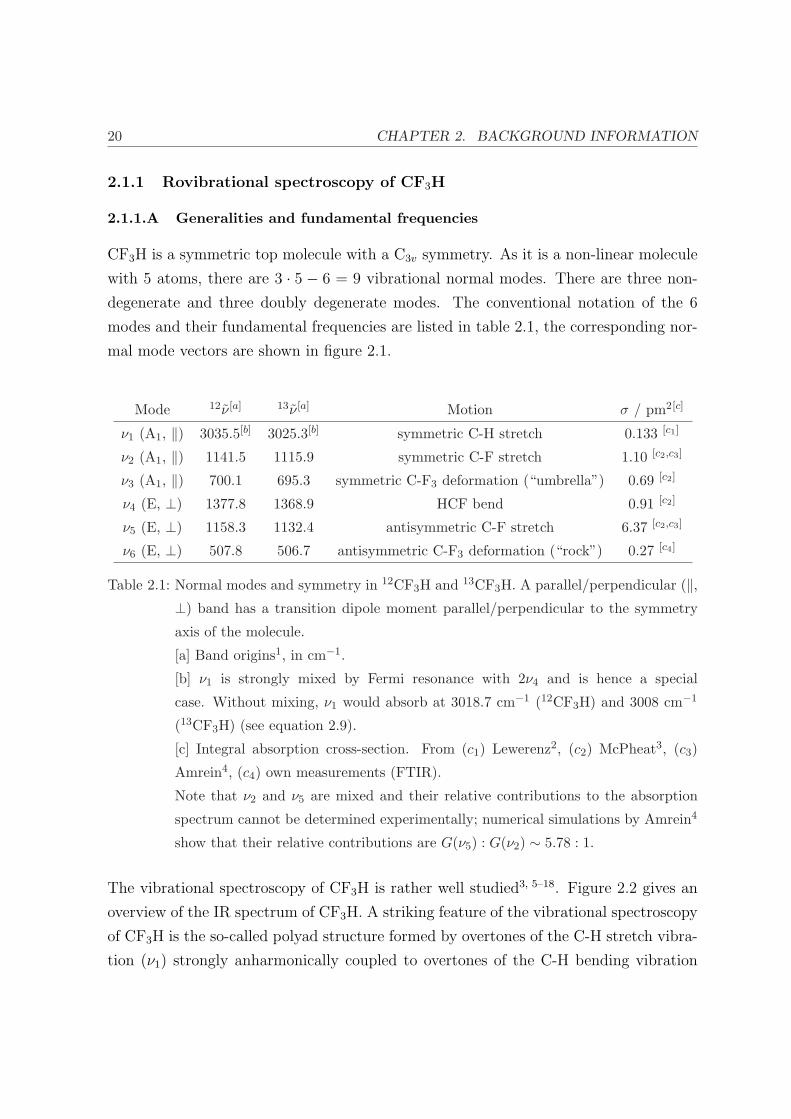
CF3H is a symmetric top molecule with a C3v symmetry. As it is a non-linear molecule
with 5 atoms, there are 3 · 5 − 6 = 9 vibrational normal modes. There are three non-
degenerate and three doubly degenerate modes. The conventional notation of the 6
modes and their fundamental frequencies are listed in table 2.1, the corresponding nor-
mal mode vectors are shown in figure 2.1.
Mode 12ν[a] 13ν[a] Motion σ / pm2[c]
ν1 (A1, ‖) 3035.5[b] 3025.3[b] symmetric C-H stretch 0.133 [c1]
ν2 (A1, ‖) 1141.5 1115.9 symmetric C-F stretch 1.10 [c2,c3]
ν3 (A1, ‖) 700.1 695.3 symmetric C-F3 deformation (“umbrella”) 0.69 [c2]
ν4 (E, ⊥) 1377.8 1368.9 HCF bend 0.91 [c2]
ν5 (E, ⊥) 1158.3 1132.4 antisymmetric C-F stretch 6.37 [c2,c3]
ν6 (E, ⊥) 507.8 506.7 antisymmetric C-F3 deformation (“rock”) 0.27 [c4]
Table 2.1: Normal modes and symmetry in 12CF3H and 13CF3H. A parallel/perpendicular (‖,⊥) band has a transition dipole moment parallel/perpendicular to the symmetry
axis of the molecule.
[a] Band origins1, in cm−1.
[b] ν1 is strongly mixed by Fermi resonance with 2ν4 and is hence a special
case. Without mixing, ν1 would absorb at 3018.7 cm−1 (12CF3H) and 3008 cm−1
(13CF3H) (see equation 2.9).
[c] Integral absorption cross-section. From (c1) Lewerenz2, (c2) McPheat3, (c3)
Amrein4, (c4) own measurements (FTIR).
Note that ν2 and ν5 are mixed and their relative contributions to the absorption
spectrum cannot be determined experimentally; numerical simulations by Amrein4
show that their relative contributions are G(ν5) : G(ν2) ∼ 5.78 : 1.
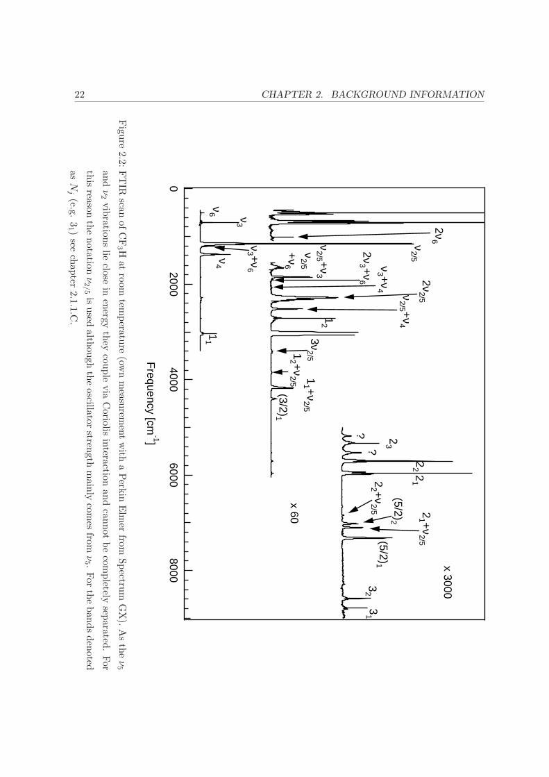
The vibrational spectroscopy of CF3H is rather well studied3, 5–18. Figure 2.2 gives an
overview of the IR spectrum of CF3H. A striking feature of the vibrational spectroscopy
of CF3H is the so-called polyad structure formed by overtones of the C-H stretch vibra-
tion (ν1) strongly anharmonically coupled to overtones of the C-H bending vibration

2.1. SPECTROSCOPY AND INTRAMOLECULAR DYNAMICS OF CF3H 21
Figure 2.1: Normal modes in CF3H (frequencies for 12CF3H).
(ν4). This will be discussed in section 2.1.1.C.
The permanent dipole moment of CF3H is d ≈ 1.65 debye19. The transition dipole
moment µ = 〈0 |d| 1〉 for a certain transition can be calculated from the integrated band
intensity, G, as follows20:
G = 41.624
( |〈0|d|1〉|Debye
)2
pm2 (2.1)
These transition dipole moments are given in table 2.2.
ν1 ν2 ν3 ν4 ν5 ν6
|〈0|d|1〉| / Debye 5.65 · 10−2 1.62 · 10−1 1.28 · 10−1 1.47 · 10−1 3.91 · 10−1 8.05 · 10−2
Table 2.2: Transition dipole moment between the ground state and the fundamentals.
22 CHAPTER 2. BACKGROUND INFORMATION
80006000
40002000
0
Frequency [cm
-1]
x 60
x 3000
ν3
ν2/5
ν3 +ν
6
ν4
ν2/5
+ν6
ν2/5 +ν
3
2ν3 +ν
6
ν3 +ν
4
2ν2/5ν
2/5 +ν4
12
11
11 +ν
2/5
(3/2)1
23
??
22
212
2 +ν2/5 2
1 +ν2/5(5/2)1
(5/2)2
31
32
12 +ν
2/5
3ν2/5
ν6
2ν6
Figure
2.2:FT
IRscan
ofC
F3 H
atroom
temperature
(own
measurem
entw
itha
Perkin
Elm
erfrom
SpectrumG
X).A
sthe
ν5
andν2
vibrationslie
closein
energythey
couplevia
Coriolis
interactionand
cannotbe
completely
separated.For
thisreason
thenotation
ν2/5
isused
althoughthe
oscillatorstrength
mainly
comes
fromν5 .
Forthe
bandsdenoted
asN
j(e.g.
31 )
seechapter
2.1.1.C.
2.1. SPECTROSCOPY AND INTRAMOLECULAR DYNAMICS OF CF3H 23
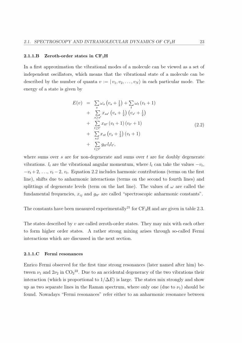
2.1.1.B Zeroth-order states in CF3H
In a first approximation the vibrational modes of a molecule can be viewed as a set of
independent oscillators, which means that the vibrational state of a molecule can be
described by the number of quanta v := | v1, v2, . . . , vN〉 in each particular mode. The
energy of a state is given by
E(v) =∑s
ωs
(vs + 1
2
)+
∑t
ωt (vt + 1)
+∑s≥s′
xss′(vs + 1
2
) (vs′ +
12
)
+∑t≥t′
xtt′ (vt + 1) (vt′ + 1)
+∑s,t
xst
(vs + 1
2
)(vt + 1)
+∑t≥t′
gtt′ltlt′ ,
(2.2)
where sums over s are for non-degenerate and sums over t are for doubly degenerate
vibrations. lt are the vibrational angular momentum, where lt can take the values −vt,
−vt +2, . . ., vt−2, vt. Equation 2.2 includes harmonic contributions (terms on the first
line), shifts due to anharmonic interactions (terms on the second to fourth lines) and
splittings of degenerate levels (term on the last line). The values of ω are called the
fundamental frequencies, xij and gtt′ are called “spectroscopic anharmonic constants”.
The constants have been measured experimentally21 for CF3H and are given in table 2.3.
The states described by v are called zeroth-order states. They may mix with each other
to form higher order states. A rather strong mixing arises through so-called Fermi
interactions which are discussed in the next section.
2.1.1.C Fermi resonances
Enrico Fermi observed for the first time strong resonances (later named after him) be-
tween ν1 and 2ν2 in CO222. Due to an accidental degeneracy of the two vibrations their
interaction (which is proportional to 1/∆E) is large. The states mix strongly and show
up as two separate lines in the Raman spectrum, where only one (due to ν1) should be
found. Nowadays “Fermi resonances” refer either to an anharmonic resonance between

24 CHAPTER 2. BACKGROUND INFORMATION
ω1 3077.0 ω2 1155.1 ω3 710.3
ω4 1396.3 ω5 1184.7 ω6 520.1
x11 -36.0 (-44.0) x12 -5.7 (-5.5) x13 4.8 (1.9)
x14 -5.1 (-54.9) x15 -7.9 (-1.0) x16 -0.6 (0.7)
x22 -7.9 (-3.4) x23 -1.6 (-2.1) x24 -1.1 (2.5)
x25 -5.6 (-0.9) x26 1.6 (-2.6) x33 -2.4 (-0.3)
x34 -0.8 (-0.8) x35 -5.7 (-3.9) x36 0.0 (-1.1)
x44 -0.5 (4.5) x45 -13.7 (-2.5) x46 -1.0 (-0.7)
x55 0.7 (-3.0) x56 -7.8 (-3.1) x66 -0.4 (-0.2)
g44 -2.3 g45 1.0 g46 0.4
g55 1.7 g56 -1.5 g66 0.3
Table 2.3: Anharmonic constants for CF3H. All values are in cm−1. The values ωi and xij are
determined experimentally. The bracketed values and the values for gij are best fit
values.
vibrational modes, which have an approximate 1:2 ratio of frequencies23 or strong an-
harmonic couplings in general24, depending on the author. In principle, there is nothing
special about a 1:2 resonance apart that it occurs quite often.
Let qi be the vibrational normal coordinate of mode i. The potential part of the molec-
ular Hamiltonian can be written as
V = V0+∑
i
(∂2V
∂q2i
)qiqj +
∑
i,j,k
(∂3V
∂qi∂qj∂qk
)qiqjqk+
∑
i,j,k,l
(∂4V
∂qi∂qj∂qk∂ql
)qiqjqkql+. . . ,
(2.3)
where the sums go from 1 to N (number of modes). In the approximation of indepen-
dent harmonic oscillators derivatives of V of order higher than 2 are zero. In a real
molecule this is not the case and it has to be taken into account for the calculation of
the energies of the molecular states. The values of (∂3V/∂qiqjqk), . . . are called “anhar-
monic constants”.
Sticking to the definition of a 1:2 resonance, a Fermi resonance is formally a third
order anharmonic coupling of the type 〈vi, vj, . . . |Vijj| vi − 1, vj + 2, . . .〉 where Vijj =

2.1. SPECTROSCOPY AND INTRAMOLECULAR DYNAMICS OF CF3H 25
∂3V/∂qi∂q2j as given in equation 2.3. The value of Vijj/∆E is a measure of the mixing
of the two states, where ∆E is the difference of the energies of the zeroth order states
| vi, vj, . . .〉 and | vi − 1, vj + 2, . . .〉. The larger this ratio is, the more important the
Fermi resonance.
Multiple peaks in an absorption spectrum arise from strong mixing of normal modes
due to Fermi resonances. To explain this, we begin with a set of (N + 1) so called
“zeroth order states” (our normal modes) which we will denote as follows:
| b〉 bright state. IR active vibration.
| di〉 dark states (i = 1, . . . , N). IR inactive vibrations.(2.4)
| b〉 and | di〉 couple to give the following eigenstates (called “first order states”):
|ψj〉 = c0,j| b〉+N∑
i=1
ci,j| di〉 (2.5)
If mixing is only weak, these first order states are often labeled the same way as the
zeroth order states, which may be confusing but nevertheless useful.
The IR transition strength between the ground state and |ψj〉 is given by
Ij ∝ |〈0 |~d|ψj〉|2
= |c0,j 〈0 |~d| b〉︸ ︷︷ ︸6=0
+N∑
i=1
ci,j 〈0 |~d| di〉︸ ︷︷ ︸=0
|2
= |c0,j〈0 |~d| b〉|2. (2.6)
Here, ~d is the dipole moment of the molecule. In such a situation, one says that |ψj〉“borrows” some transition strength from | b〉. In a spectrum one will see a set of N + 1
peaks corresponding to the | 0〉 → |ψj〉 transitions. This set of N + 1 peaks is called
a “polyad” (or “diad” if only two states couple, “triad” if three states couple, and so
on). Experimentally one can measure the values of |c0,j|2 by measuring the absorption
strengths of the different members of a polyad and using the relation established in
equation 2.6, i.e. Ij ∝ |c0,j|2. Figure 2.3 shows a schematic example of the effect of
state mixing on the spectrum.

26 CHAPTER 2. BACKGROUND INFORMATION
Figure 2.3: Anharmonic coupling between dark and bright states give rise to a polyad structure
in the absorption spectra. The figure on the left would apply to a system of one
bright state | b〉 and a set of N dark states | di〉 in the absence of interactions.
The horizontal lines represent the states, the dark part of the line represents the
brightness of a state (i.e. what can be seen in an absorption spectrum). The figure
on the right corresponds to the same system but including anharmonic coupling.
The levels are shifted, and the bright part of a state is taken from | b〉.
2.1.1.D Fermi resonances in CF3H
The first observation of a Fermi resonance in CF3H was made in 1948 by Bernstein and
Herzberg5. They identified a peak at 8792 cm−1 to be 3ν1 and a peak at 8589 cm−1 to
be 2ν1 + 2ν4, and the possibility of mixing through Fermi resonances has been correctly
suggested by the authors.
We will apply the formalism introduced in the previous section to CF3H. In this molecule,
the ν1 and 2ν4 vibrations accidentally lie close to each other (∼3,000 cm−1). Their cou-

2.1. SPECTROSCOPY AND INTRAMOLECULAR DYNAMICS OF CF3H 27
pling is appreciable, which gives rise to polyads discussed above. The ν1 vibration, | b〉, is
IR active whereas the 2ν4 vibration, | d〉, is, at least in the harmonic approximation, not.
Using the notation | x, y〉 = |n1 = x, n4 = y〉, the | 1, 0〉 and the | 0, 2〉 states couple
with each other and form first order states:
|ψ0〉 = c0,0| 1, 0〉+ c1,0| 0, 2〉|ψ1〉 = c0,1| 1, 0〉+ c1,1| 0, 2〉
(2.7)
Higher overtones couple in a similar manner: e.g. | 3, 0〉, | 2, 2〉, | 1, 4〉 and | 0, 6〉 couple
to form following eigenstates:
|ψj〉 = c0,j| 3, 0〉+ c1,j| 2, 2〉+ c2,j| 1, 4〉+ c3,j| 0, 6〉 (2.8)
One denotes the first order states |ψj〉 per definition as |Nx〉, where N is the number of
quanta in the zeroth order C-H stretch vibration, and x is 1, 2, . . . where “1” stands for
the state with the highest energy, “2” for the state with the second highest energy, etc20.
Due to the Fermi resonance structure, the C-H stretch vibration and its overtones have
received a lot of experimental17, 20, 25–33 and theoretical attention. Quack and co-workers
have extensively analysed the polyad structure of the CH chromophore in CF3H17, 20, 25.
They propose a tridiagonal structure of the matrix linking the states coupled by Fermi
resonances. They define a “chromophore level N” to be the set of normal modes with
a particular N = v1 + 12v4. Working in the normal mode basis set, |N, 0〉, |N − 1, 2〉,
. . . | 0, 2N〉, the matrix elements for a given chromophore are given as follows‡:
〈v1, v4 |H| v1, v4〉 = ν ′sv1 + ν ′bv4 + x′ssv21 + x′bbv
24 + x′sbv1v4
〈v1, v4 |H| v1 − 1, v4 + 2〉 = −12ksbb (v4 + 2)
√12v1 ,
(2.9)
where H is the molecular Hamiltonian.
All other matrix elements are zero. Least square fits have been performed20, 25 to get
‡Quack also includes the vibrational angular momentum lb in the notation. As long as we work with
N = 1, 2, 3, . . . this value is lb = 0 and can be left away from the notation. For half-integer values of N we have
lb = 1 and the values for off-diagonal matrix elements change, but the fundamental ideas and developments are
the same. In our explanations we will omit the angular momentum for simplicity.
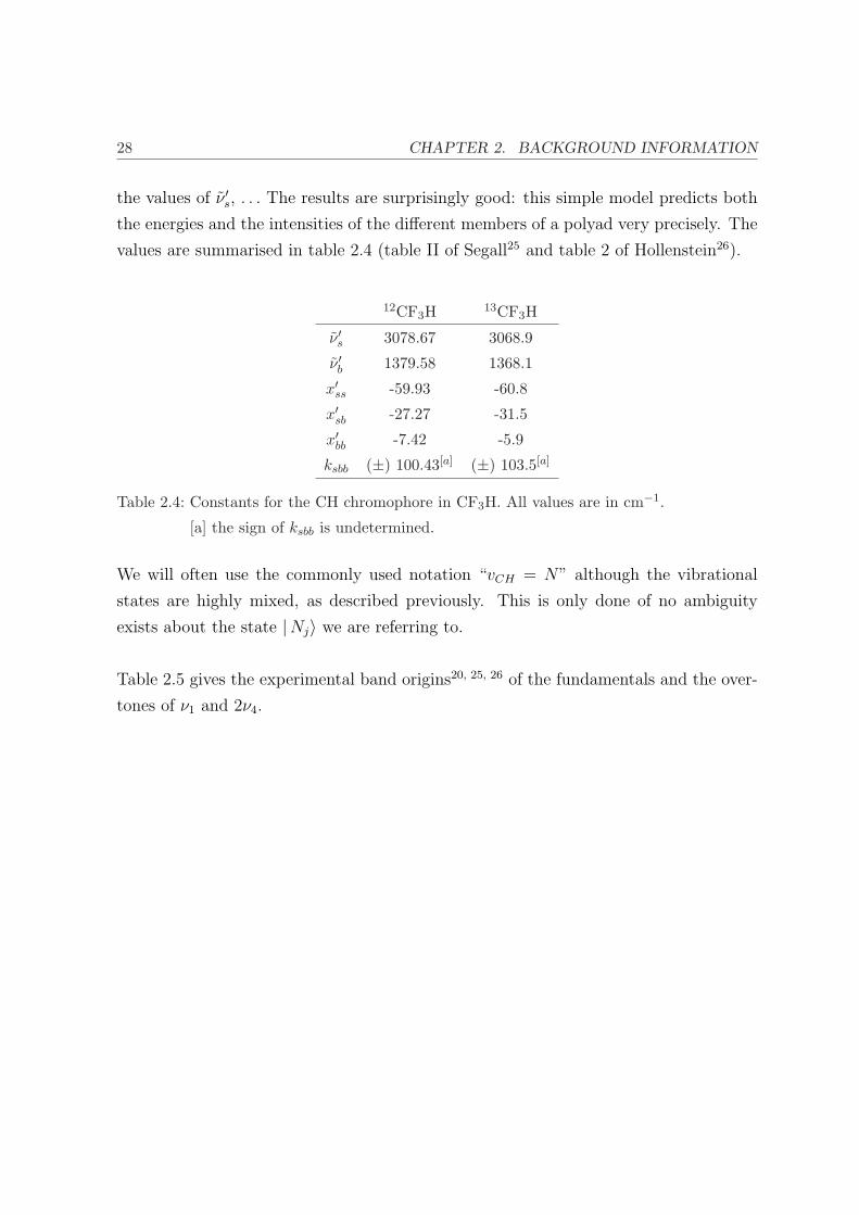
28 CHAPTER 2. BACKGROUND INFORMATION
the values of ν ′s, . . . The results are surprisingly good: this simple model predicts both
the energies and the intensities of the different members of a polyad very precisely. The
values are summarised in table 2.4 (table II of Segall25 and table 2 of Hollenstein26).
12CF3H 13CF3H
ν ′s 3078.67 3068.9
ν ′b 1379.58 1368.1
x′ss -59.93 -60.8
x′sb -27.27 -31.5
x′bb -7.42 -5.9
ksbb (±) 100.43[a] (±) 103.5[a]
Table 2.4: Constants for the CH chromophore in CF3H. All values are in cm−1.
[a] the sign of ksbb is undetermined.
We will often use the commonly used notation “vCH = N” although the vibrational
states are highly mixed, as described previously. This is only done of no ambiguity
exists about the state |Nj〉 we are referring to.
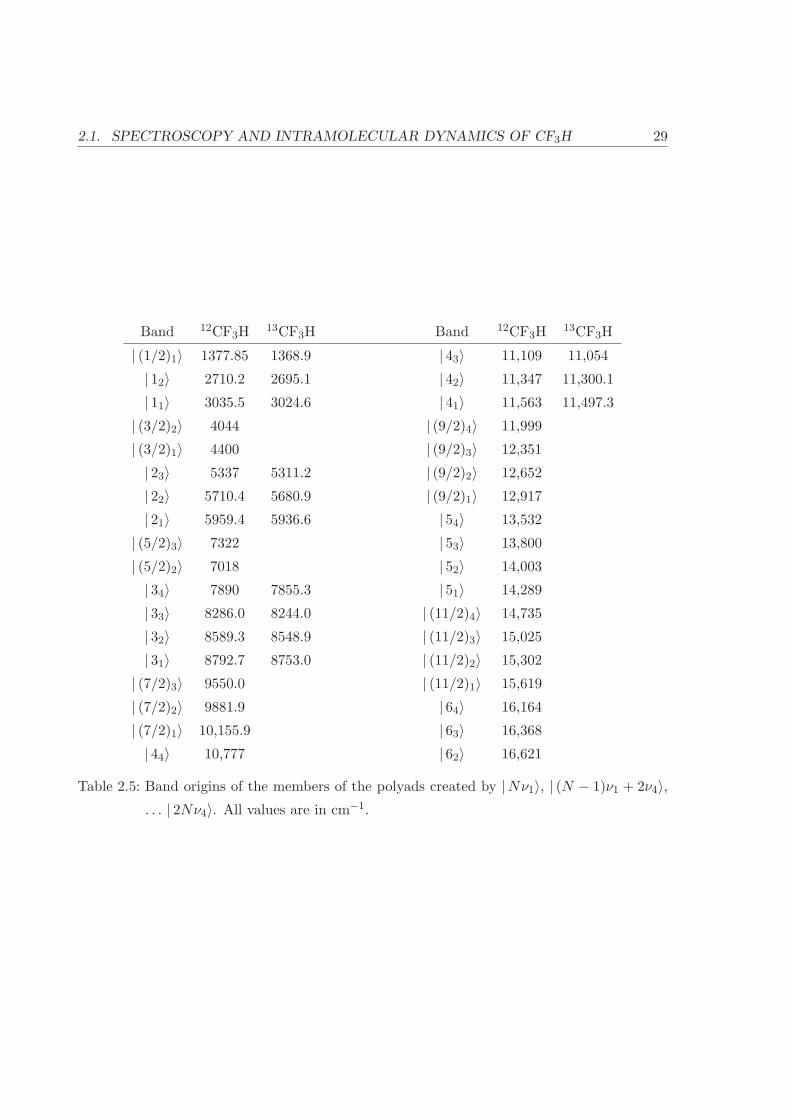
Table 2.5 gives the experimental band origins20, 25, 26 of the fundamentals and the over-
tones of ν1 and 2ν4.
2.1. SPECTROSCOPY AND INTRAMOLECULAR DYNAMICS OF CF3H 29
Band 12CF3H 13CF3H Band 12CF3H 13CF3H
| (1/2)1〉 1377.85 1368.9 | 43〉 11,109 11,054
| 12〉 2710.2 2695.1 | 42〉 11,347 11,300.1
| 11〉 3035.5 3024.6 | 41〉 11,563 11,497.3
| (3/2)2〉 4044 | (9/2)4〉 11,999
| (3/2)1〉 4400 | (9/2)3〉 12,351
| 23〉 5337 5311.2 | (9/2)2〉 12,652
| 22〉 5710.4 5680.9 | (9/2)1〉 12,917
| 21〉 5959.4 5936.6 | 54〉 13,532
| (5/2)3〉 7322 | 53〉 13,800
| (5/2)2〉 7018 | 52〉 14,003
| 34〉 7890 7855.3 | 51〉 14,289
| 33〉 8286.0 8244.0 | (11/2)4〉 14,735
| 32〉 8589.3 8548.9 | (11/2)3〉 15,025
| 31〉 8792.7 8753.0 | (11/2)2〉 15,302
| (7/2)3〉 9550.0 | (11/2)1〉 15,619
| (7/2)2〉 9881.9 | 64〉 16,164
| (7/2)1〉 10,155.9 | 63〉 16,368
| 44〉 10,777 | 62〉 16,621
Table 2.5: Band origins of the members of the polyads created by |Nν1〉, | (N − 1)ν1 + 2ν4〉,. . . | 2Nν4〉. All values are in cm−1.

30 CHAPTER 2. BACKGROUND INFORMATION
The individual members of a polyad (with integer N ’s) are given by
|Nj〉 =N∑
i=0
cNi,j| i, 2(N − i)〉. (2.10)
Table 2.6 gives the values of cNi,j for N ≤ 4.
N = 1 | 1, 0〉 | 0, 2〉| 11〉 0.97 -0.23
| 12〉 0.23 0.97
N = 2 | 2, 0〉 | 1, 2〉 | 0, 4〉| 21〉 0.92 -0.39 0.10
| 22〉 0.40 0.83 -0.40
| 23〉 0.07 0.41 0.91
N = 3 | 3, 0〉 | 2, 2〉 | 1, 4〉 | 0, 6〉| 31〉 0.77 -0.57 0.27 -0.08
| 32〉 0.61 0.53 -0.55 0.22
| 33〉 0.18 0.60 0.58 -0.52
| 34〉 0.03 0.18 0.54 0.82
N = 4 | 4, 0〉 | 3, 2〉 | 2, 4〉 | 1, 6〉 | 0, 8〉| 41〉 -0.48 0.64 -0.52 0.27 0.09
| 42〉 0.78 0.03 -0.46 0.39 -0.16
| 43〉 0.39 0.66 0.11 -0.55 0.33
| 44〉 0.10 0.38 0.64 0.31 -0.58
| 45〉 0.01 0.09 0.30 0.61 0.72
Table 2.6: Values of ciN,J defined in equation 2.10 for 12CF3H (there are very small differences
between the two isotopomers).
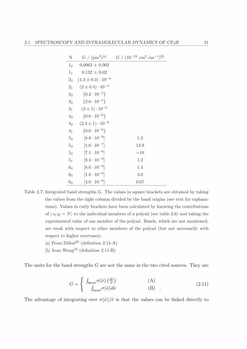
The integrated band strengths of the ν1 fundamental and its overtones are given in
table 2.7.
2.1. SPECTROSCOPY AND INTRAMOLECULAR DYNAMICS OF CF3H 31
N G / (pm2)[a] G / (10−24 cm2 cm−1)[b]
12 0.0063 ± 0.002
11 0.132 ± 0.02
22 (1.3± 0.3) · 10−4
21 (2± 0.4) · 10−4
33 0.2 · 10−532 2.6 · 10−531 (3± 1) · 10−5
43 0.6 · 10−642 (2.4± 1) · 10−6
41 0.6 · 10−654 [8.8 · 10−9] 1.2
53 [1.0 · 10−7] 13.9
52 [7.1 · 10−8] ∼10
51 [8.4 · 10−9] 1.2
64 [8.6 · 10−9] 1.4
63 [1.8 · 10−8] 3.0
62 [4.0 · 10−9] 0.67
Table 2.7: Integrated band strengths G. The values in square brackets are obtained by taking
the values from the right column divided by the band origins (see text for explana-
tions). Values in curly brackets have been calculated by knowing the contributions
of | vCH = N〉 to the individual members of a polyad (see table 2.6) and taking the
experimental value of one member of the polyad. Bands, which are not mentioned,
are weak with respect to other members of the polyad (but not necessarily with
respect to higher overtones).
[a] From Dubal20 (definition 2.11-A)
[b] from Wong34 (definition 2.11-B)
The units for the band strengths G are not the same in the two cited sources. They are
G =
∫band
σ(ν)(
dνν
)(A)∫
bandσ(ν)dν (B) .
(2.11)
The advantage of integrating over σ(ν)/ν is that the values can be linked directly to

32 CHAPTER 2. BACKGROUND INFORMATION
basic molecular quantities, such as the transition dipole moment (see equation 2.1). A
rough conversion between the two units can be done by multiplying or dividing by the
band origin ν0.
After conversion between the two units the integral band strengths are summed over a
polyad to get the transition strengths | 0〉 → |N, 0, . . .〉 which are shown in figure 2.4.
If the strength of the | 0〉 → | 1〉 absorption is normalised to 1, the strengths for the
transitions to | 2〉, . . ., | 6〉 are well described by the equation
G (0 → vCH = N) = 0.56 · exp (−1.03 ·N) (2.12)
using definition (A) of equation 2.11.
-6
-4
-2
0
Log
(Int
egra
l abs
orpt
ion
stre
ngth
) [a
.u.]
654321
N
Figure 2.4: Integrated absorption strengths of 0 → νCH = N .
2.1.1.E Rotational contours
Analysis of the different rovibrational fundamental bands in CF3H have been carried
out in a number of previous works. Most of the bands exhibit a relatively clean ro-
tational structure. An exception is the ν5 fundamental, which has received particular

2.1. SPECTROSCOPY AND INTRAMOLECULAR DYNAMICS OF CF3H 33
attention4, 10, 18, 29, 35 because of Coriolis interaction with ν2.
CF3H is an oblate symmetric top molecule, its rotational contour is hence (mainly)
characterised by the rotational constants B and C. The rotational states are well de-
scribed by the quantum numbers J and K. On a low level of accuracy the rotational
levels are given by
F (J,K) = ν0(v) + B · J · (J + 1) + (C −B) ·K2, (2.13)
where ν0(v) is the band origin given in equation 2.2. The rotational constants B and C
depend on the vibrational excitation v. B and C can be described by
B = B0 −6∑
i=1
αBi
(vi +
di
2
)(2.14)
and similarly for C where di is the degeneracy of vibration i (1 for i = 1-3, 2 for i =
4-6). The values of αBi and αC
i have been measured25 and are given in table 2.8.
α1 α2 α3 α4 α5 α6
B 1.4 4.116 6.463 4.1 12.457 -1.217
C 0.4 4.7811 1.7 0.8 5.529 3.418
Table 2.8: αi · 103 for B and C for CF3H.
2.1.2 IVR
2.1.2.A Generalities about IVR
IVR23, 36–38 is the abbreviation for “Intramolecular Vibrational Energy Redistribution”.
In a “classical” (time-resolved) picture, IVR is the process by which vibrational energy
deposited in a localised vibration of the molecule redistributes over the whole system.
The time-scale for the molecule to redistribute the energy is denoted as τIVR. The
importance of IVR was first noticed in unimolecular reaction studies39. Later, observa-
tions in experiments involving IR multiple photon dissociation40 (IRMPD) could only
be explained using the concept of rapid (∼ps time-scale) energy redistribution from the
pumped mode to the rest of the molecule. Realising the influence of IVR moderated

34 CHAPTER 2. BACKGROUND INFORMATION
hopes of mode selective chemistry and opened at the same time a new field of research.
The questions are: to what extent (under what conditions) and how fast does IVR take
place ?
The explanation of IVR given above is clarified and formalised if one thinks about
the problem in frequency space rather than in time. A narrow band laser excites a
single eigenstate of the molecule which is by definition stationary. A short broadband
laser however excites a coherent superposition of two or more eigenstates, which is not
an eigenstate itself. In this case, the state will evolve over time. Bearing in mind that
a short laser pulse corresponds to a broadband laser (and a long pulse corresponds to
a narrowband laser) one immediately sees that exciting the system with a pulse with
τ ¿ τIVR corresponds to a spectral width of ∆νlaser/hc ∼ h/τ À ∆ν/hc where ∆ν is
the spacing between the eigenstates.
Figure 2.5: IVR
A small example shall illustrate this. Assume two states | b〉 and | d〉 where | b〉 carries

2.1. SPECTROSCOPY AND INTRAMOLECULAR DYNAMICS OF CF3H 35
all the oscillator strength and assume them coupled forming the eigenstates
|ψ0〉 = c0,0| b〉+ c1,0| d〉|ψ1〉 = c0,1| b〉+ c1,1| d〉 .
(2.15)
Exciting the molecule with a short (and broad) laser pulse excites |Ψ〉 which can be
expressed in terms of the eigenstates
|Ψ(t = 0)〉 = | b〉 = c0|ψ0〉+ c1|ψ1〉 (2.16)
and its evolution is described as
|Ψ(t)〉 = c0eE0it/~|ψ0〉+ c1e
E1it/~|ψ1〉 (2.17)
and the probability of finding the molecule in its initial state is
P (t) = |〈Ψ(t) |Ψ(0)〉|2= ||c0|2eE0it/~ + |c1|2eE1it/~|2= |c0|4 + |c1|4 + 2|c0|2|c1|2 cos
((E0−E1)t
~
).
(2.18)
The state evolves and oscillates between | b〉 and a certain superposition of | b〉 and | d〉.If |c0| = |c1| = 1/
√2 there is a complete oscillation between | b〉 and | d〉. In the case
of many bath states | di〉 coupled to | b〉, the population in | b〉 approximately decays
exponentially (the formalism gets slightly more complicated, but the mechanism stays
the same).
The generalisation from the case of two coupled states |ψ1〉 and |ψ2〉 to multiple cou-
pled states |ψ1〉, |ψ2〉, . . . |ψn〉 is (at least in principle) straightforward. These states
are sometimes referred to as “zeroth order states”. They are obtained neglecting the
interaction terms amongst each others and only represent an approximation to the real
eigenstate. The time-scale for IVR is the time during which this approximation holds
well. |Ψ1〉, |Ψ2〉, . . ., the states that are obtained without neglecting the interactions
between |ψ1〉, |ψ2〉, . . ., are sometimes referred to as “first order states”. If these first
order states are further (weaker) coupled to other states, this gives in a similar manner
rise to second order states (and so on). In this case, the first order states are good ap-
proximations to the real eigenstates during the time-scale of this second flow of energy.

36 CHAPTER 2. BACKGROUND INFORMATION
This can give rise to multiple time-scales for energy flow within a molecule.
Probing IVR dynamics can be done either in time resolved or in frequency resolved
experiments. Both methods should, in principle, yield the same results. In general
frequency resolved measurements are preferred37, 38 because they contain all necessary
information to investigate IVR dynamics. When performing time-resolved experiments
one starts with ill-defined states which complicate the analysis considerably.
As a rule of thumb38 IVR becomes important at a density of states ρ of 10-100 states / cm−1.
However, whether IVR at a certain energy is important or not depends on the particular
experiment in question. We will illustrate this for the example of IR multiple photon
excitation (IRMPE - see section 2.2). Here molecules absorb several photons and gain
more and more vibrational energy. The vibrational levels at every level of excitation
are mixed, but the time-scales for the energy redistribution depend on the vibrational
energy; in general one can say that the higher the density of states, the shorter the
time-scales on which the energy flows out of a vibrational mode to other close lying
levels (although this is not strictly true). The importance of IVR depends on the time-
scales of the experiment in question; in the case of IRMPE the molecule goes through
energy regions with increasing density of states and will at a given energy reach a region
where IVR is faster than the time-scale of the experiment. We will call this energy Est.
Experimental measurements with a CO2 laser by Ryabov and coworkers show that the
transition to the regime where IVR is very fast with respect to typical ns experiments is
rather abrupt, i.e. Est is, at least in principle, rather well defined. For small polyatomic
molecules this value lies around (5− 8) · 103 cm−1. Thresholds have been determined41
for SF6 ((5000 ± 500) cm−1), CF3Br ((7500 ± 300) cm−1), CF3I (≤ 6000 cm−1), CF2HCl
((4-5) ·103 cm−1) and CF2Cl2 (≤ 7800 cm−1).
Experimental studies of highly excited small polyatomic molecules over the past decade
have resulted in a better comprehension of IVR at high energies. There is a general
trend is that the IVR rate Γ goes up as the density of states ρ increases, but there is
no monotonic dependence between the two values37, 38 although Fermi’s Golden Rule,
Γ = 2π|〈W 〉|2ρ/~, may suggest this (|〈W 〉|2 is the square of the average coupling be-
tween the bright state and the bath states it is immerged in). As one goes up in energy

2.1. SPECTROSCOPY AND INTRAMOLECULAR DYNAMICS OF CF3H 37
ρ is increased, at the same time |〈W 〉|2 decreases as large changes in vibrational quan-
tum numbers must occur between the coupled states. It turns out, that the two effects
roughly cancel out.
2.1.2.B IVR in CF3H
After the fast redistribution of energy within the C-H stretch and bend motions in
CF3H, the energy stays localised for a certain time within these vibrations before it is
redistributed over the rest of the molecule. In section 2.1.1.C the fast redistribution has
been discussed. The large splitting in the order of several 100’s of cm−1 indicates redis-
tribution times of 30-100 fs. In order to investigate the vibrational energy redistribution
out of the C-H stretch bend vibrations to the rest of the molecule, higher resolution
spectra of single bands are necessary. The widths or splittings of the transition bands
give information on vibrational redistribution from the first order states defined previ-
ously to second order states. In our case, the states belonging to different tiers of states
are given in table 2.9.
Order of tier States
Zeroth order |n1 = 3〉, |n1 = 2, n4 = 2〉, |n1 = 1, n4 = 4〉, |n4 = 6〉First order 31, 32, 33, 34
Second (and higher) order unknown
Table 2.9: Tiers of states in CF3H
In the case of low state density, the first order state is coupled to one or few other states
in its vicinity, and the redistribution occurs on time-scales of τ ∼ 1/2π∆νc (where ∆ν
is the splitting of single peaks). In the case of coupling to a dense bath of states this
time is τ ∼ 1/2πγc where γ is the half Lorentzian width of the peak after deconvolu-
tion with other broadenings (width of laser, pressure / doppler broadening, ...). This is
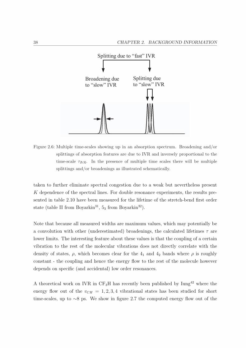
schematically shown in figure 2.6.
In two papers31, 32 such spectra have been reported for some of the overtones of the C-H
stretching vibration in CF3H. Spectral simplifications have been achieved by cooling
the molecules down to ∼8K in a jet. In some cases double resonance spectra have been
38 CHAPTER 2. BACKGROUND INFORMATION
Figure 2.6: Multiple time-scales showing up in an absorption spectrum. Broadening and/or
splittings of absorption features are due to IVR and inversely proportional to the
time-scale τIVR. In the presence of multiple time scales there will be multiple
splittings and/or broadenings as illustrated schematically.
taken to further eliminate spectral congestion due to a weak but nevertheless present
K dependence of the spectral lines. For double resonance experiments, the results pre-
sented in table 2.10 have been measured for the lifetime of the stretch-bend first order
state (table II from Boyarkin31, 53 from Boyarkin32).
Note that because all measured widths are maximum values, which may potentially be
a convolution with other (underestimated) broadenings, the calculated lifetimes τ are
lower limits. The interesting feature about these values is that the coupling of a certain
vibration to the rest of the molecular vibrations does not directly correlate with the
density of states, ρ, which becomes clear for the 41 and 42 bands where ρ is roughly
constant - the coupling and hence the energy flow to the rest of the molecule however
depends on specific (and accidental) low order resonances.
A theoretical work on IVR in CF3H has recently been published by Iung42 where the
energy flow out of the vCH = 1, 2, 3, 4 vibrational states has been studied for short
time-scales, up to ∼8 ps. We show in figure 2.7 the computed energy flow out of the
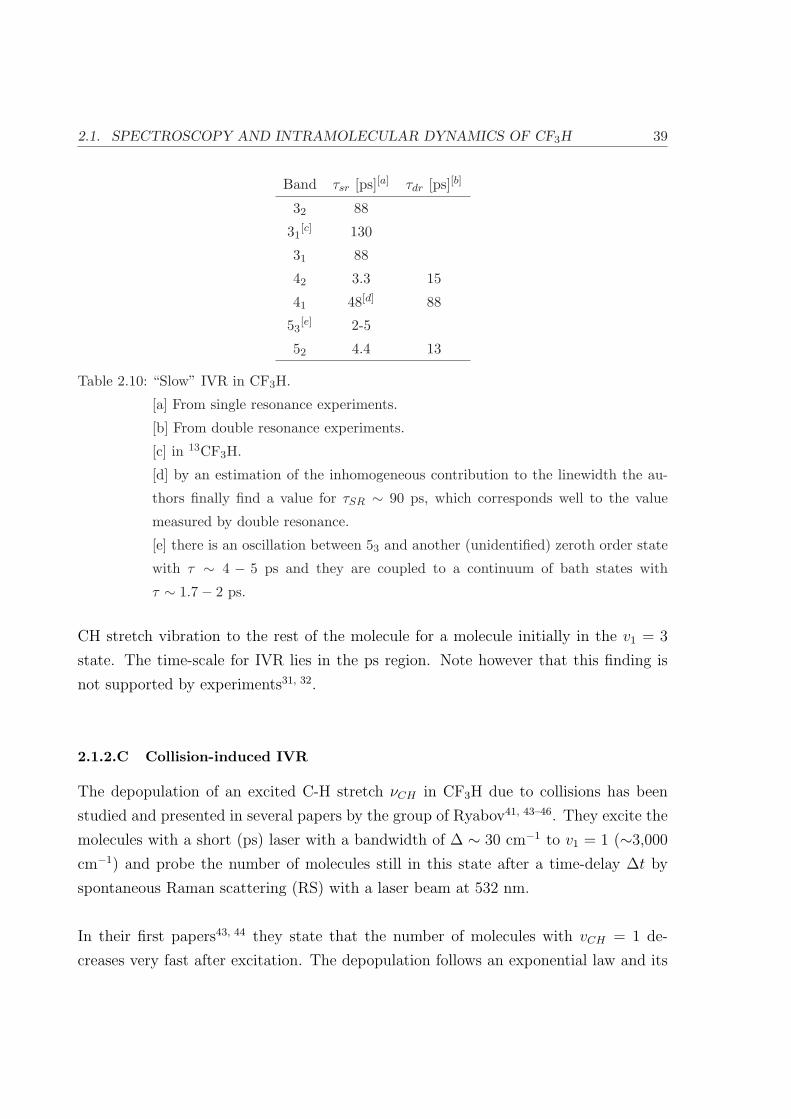
2.1. SPECTROSCOPY AND INTRAMOLECULAR DYNAMICS OF CF3H 39
Band τsr [ps][a] τdr [ps][b]
32 88
31[c] 130
31 88
42 3.3 15
41 48[d] 88
53[e] 2-5
52 4.4 13
Table 2.10: “Slow” IVR in CF3H.
[a] From single resonance experiments.
[b] From double resonance experiments.
[c] in 13CF3H.
[d] by an estimation of the inhomogeneous contribution to the linewidth the au-
thors finally find a value for τSR ∼ 90 ps, which corresponds well to the value
measured by double resonance.
[e] there is an oscillation between 53 and another (unidentified) zeroth order state
with τ ∼ 4 − 5 ps and they are coupled to a continuum of bath states with
τ ∼ 1.7− 2 ps.
CH stretch vibration to the rest of the molecule for a molecule initially in the v1 = 3
state. The time-scale for IVR lies in the ps region. Note however that this finding is
not supported by experiments31, 32.
2.1.2.C Collision-induced IVR
The depopulation of an excited C-H stretch νCH in CF3H due to collisions has been
studied and presented in several papers by the group of Ryabov41, 43–46. They excite the
molecules with a short (ps) laser with a bandwidth of ∆ ∼ 30 cm−1 to v1 = 1 (∼3,000
cm−1) and probe the number of molecules still in this state after a time-delay ∆t by
spontaneous Raman scattering (RS) with a laser beam at 532 nm.
In their first papers43, 44 they state that the number of molecules with vCH = 1 de-
creases very fast after excitation. The depopulation follows an exponential law and its

40 CHAPTER 2. BACKGROUND INFORMATION
Figure 2.7: Calculated redistribution of vibrational energy in a CF3H molecule initially in the
v1 = 3 state42.
— ν1, – - – ν4, - - - CH chromophore, bullets: other modes.
There is an initial fast energy flow from ν1 to ν4, and from there to the rest of the
molecule on the time-scale of ∼ 1ps.
Reproduced from Iung42 (figure 2).
rate of 1.67 ·107 s−1 torr−1 exceeds the gas kinetic rate by a factor of ∼1.5. This means
that it necessitates on average 0.7 collisions for the loss of one quantum in νCH which
is unexpectedly low: non-resonant V-V’ energy transfer necessitates in general at least
10 collisions, resonant V-V energy transfer typically requires a couple of collisions47.
Later45, 46 the relaxation experiments were performed with buffer gases (He, Kr, Xe,
N2, SO2, H2S) where any V-V or V-V’ energy transfer can be excluded. Neither can
the loss of energy in the excited mode νCH be attributed to IVR of the isolated molecule.
This decrease of the average population of v1 = 1 has been attributed to “Collision-
induced IVR” (CI-IVR), i.e. the presence of another molecule or atom perturbs the
molecule in such a way that rapid IVR is initiated. Formal considerations can also be

2.2. IR MULTIPLE PHOTON DISSOCIATION (IRMPD) 41
found in the literature48, 49.
2.2 IR multiple photon dissociation (IRMPD)
In this section we discuss IR multiple photon dissociation (IRMPD). First, we give a brief
historical overview about IRMPD, then we qualitatively describe different aspects of
IRMPD, and finally we give a quantitative description based on a statistical treatment.
2.2.1 Some history
Infrared multiple photon dissociation (IRMPD) is a key feature of the method we em-
ploy for the isotope separation process. First observations50–53 of MPD were carried
out in the 1960’s on NH3, SF6, hydrocarbons, Br2 or BCl3 in the presence of collisions
between the molecules. This was a direct consequence of the development of powerful
CW CO2 lasers in the 9.2 - 10.8 µm (920-1090 cm−1) region. All authors suggested that
collisions during IRMPD inducing rotational relaxation were necessary for the whole
process to be efficient. The argumentation was that for molecules to be pumped up
to the dissociation threshold, each step required a different wavelength if no change in
rotational quantum numbers due to collisions occurs between the absorption steps.
Later, in 1974, it was found independently by two research groups that IRMPD can
also be efficient under collision-less conditions54, 55. Explanations of why IRMPD is so
efficient in collision-less conditions exist56 although finer details are still missing up to
date.
The first observation of isotopically selective dissociation was made in 1974 on BCl357
and was confirmed later for other molecules such as SF6, CCl4 or OsO4. A plethora
of studies on IRMPD of small molecules and isotopic selectivity has been published
because of the possibility of using this method for molecular laser isotope separation
(MLIS) on an industrial scale.

42 CHAPTER 2. BACKGROUND INFORMATION
2.2.2 Qualitative description
In general a qualitative image where IRMPD of ground state molecules is composed by
two distinct steps is widely accepted40, 58. This image is depicted in figure 2.8.
Region I: low density of states
Region II: high density of states
Figure 2.8: While a molecule undergoes IRMPD it is pumped through two qualitatively dis-
tinct regions. In region I the density of states (DOS) is low and the absorption
has a resonant character, in region II the DOS is high and the absorption is not
very wavelength sensitive any more.
The first steps, starting in the ground state of the molecule and leading up to a certain
stochastic limit (see comment on page 36), is the natural bottleneck for IRMPD, be-
cause the molecule exhibits a relatively low density of states (DOS) in this region, which
gives IR absorption a resonant character (region I in figure 2.8). For CF3H we estimate
this limit to be around Est ∼ 7000 cm−1. The individual steps through the energy
region with low DOS have different efficiencies because the frequencies with the highest
absorption cross-section shift upon excitation of the molecule due to anharmonicity.
This bottleneck can be overcome with high power laser pulses which cause substantial
power broadening.
The subsequent steps of IRMPD happen in what is called the “vibrational quasi-
2.2. IR MULTIPLE PHOTON DISSOCIATION (IRMPD) 43
continuum” (region II in figure 2.8). It is not a continuum in the strict sense, but
the DOS is sufficiently high, that there is always a resonant transition within the band-
width of the dissociating laser. This is because states that are close in energy mix
strongly. Because of this strong mixing there is a broadening of the absorption spectra
(see section 5.1.1) which makes pumping through this region relatively easy.
2.2.3 Quantitative description
We have previously described IRMPD on a qualitative level. In this section we will
describe it quantitatively. First, we give a brief overview regarding the possibility of
finding an exact solution and then describe a simplified approach based on a statistical
treatment.
2.2.3.A Exact problem and approximate solutions
We are interested in knowing the evolution of a molecule in the presence of an external
electromagnetic field ~E. The wavefunction |ψ〉 is the solution of the time-dependent
Schrodinger equation
i~∂
∂t|ψ〉 = H|ψ〉, (2.19)
where H is the Hamiltonian composed of Hmol (Hamiltonian of the isolated molecule)
and Hint (interaction with the electromagnetic field). The interaction term is given by
Hint = −~d · ~E, (2.20)
where ~d is the electric dipole moment of the molecule and ~E is the external electric field.
It is clear that in general numerical, let alone analytical solutions of the Schrodinger
equation are difficult to find.
There are some approximations that can be made to simplify the problem. One can
use Floquet’s theorem59 with which the problem can be separated to a time-dependent
and a time-independent part. A “weak field quasi-resonant approximation” (WFQA)
allows further simplification of the problem.
There are, in principle, two problems associated with these approaches. First, the

44 CHAPTER 2. BACKGROUND INFORMATION
molecular Hamiltonian is in most cases unknown. Secondly, even if we knew the Hamil-
tonian, there is a problem of computing power: the number of coupled equations grows
enormously with the number of atoms, and an exact solution can be done on reasonable
time-scales only for diatomics or at most triatomics.
In our case we will mainly deal with vibrationally hot polyatomic molecules. These
molecules have internal energies high enough for them to be well distributed over all
molecular vibrations, i.e. IVR is complete. At these energies, the molecules have a
statistical behaviour, and we can make some simplifications which we present in the
next section.
2.2.3.B Statistical treatment
The molecule we are interested in, CF3H, has five atoms and cannot be treated by the
equations and approximations cited previously, because the number of coupled states
gets enormous (CF3H has ∼ 3 ·106 vibrational states below the dissociation limit which
is at ∼24,000 cm−1). It is hence unthinkable to treat such a system even with the most
powerful computing force on reasonable time-scales.
(I) General ideas
We base our ideas on the following statistical treatment formulated by Martin Quack60–72.
A good summary of the development of the theory of a statistical treatment can be found
in a review by Letokhov73. In this treatment, vibrational states with similar energies are
binned together into “grained” energy states with a certain width ∆. The vibrational
states lose their identity and now are simply represented by their bin number I (small
letters i, j, . . . refer to the individual vibrational levels and capital letters I, J , . . . refer
to the grained levels). In other words, the state of a molecule is not characterised by its
wavefunction or by quantum numbers but by the total energy E. All members of bin I
are populated with the same probability if the molecule has an energy that falls into this
bin. In the presence of absorption or stimulated emission of a photon, the population
of the different bins will change due to up- and down-pumping. Formulae, which will
be presented below, have been developed60, 63 in order to calculate the population and
depopulation rates of the bins. Figure 2.9 shows the basic idea of a statistical treatment.

2.2. IR MULTIPLE PHOTON DISSOCIATION (IRMPD) 45
Figure 2.9: Basic idea of the statistical treatment: close lying levels are binned into grained
levels 0, 1, . . . , I − 1, I, I + 1, . . . , J, . . .. The populations pI(t) of the grained levels
reflect the number of molecules having a certain corresponding energy. KI,J is the
transition rate between level I and level J . In general J denotes the upper and I
the lower level.
We will not present the entire development of the formulae. For this the reader is
referred to the original literature60, 63. Parts will be explained in appendix A. The
notations presented in table 2.11 will be used.
Depending on the average density of states ρ = 1/δ in the bins I and J and the
average coupling between them, four different cases can be distinguished in which large
simplifications can be done:
Case A: Pumping from a single level to a set of different uncoupled levels.

46 CHAPTER 2. BACKGROUND INFORMATION
Notation used
∆I - width of a grained level I
δI - average spacing between vibrational levels in bin I
|V | - average coupling between lower and upper vibrational levels
|V | := √〈|VJ,I |2〉ω - energy of photon
pI(t) - population of level I
KX,Y - transition rate from level X to level Y
Table 2.11: Notation used for the statistical treatment (see also fig 2.9).
Case B: Pumping between sets of levels that are coupled amongst each other through
the laser field.
Case C: Pumping between sets of levels that are uncoupled amongst each other (within
a bin). The only coupling is due to the radiation field between single states of the
upper and the lower bin; this radiation is not strong enough to couple states within
a bin.
Case D: Pumping between sets of levels that are coupled amongst each other (within
a bin) with a very high power laser.
Table 2.12 summarises the conditions and pumping rates for the four different cases.

2.2. IR MULTIPLE PHOTON DISSOCIATION (IRMPD) 47
Case A Case B Case C Case D
KI,J 2π |V |2
δJ2π |V |
2
δJ2π |V |
2
δJαπ
√|V |2[a]
KI,J
KJ,I∞ δI
δJ
(δIδJ
)(π√
3|V |2δJ
)[b]1[b]
Dependence on the ini-
tial distribution of pop-
ulation ?
No No Yes Yes
Conditions[c] δI > |V | > δJ ∆ > |V | > δ |V | > δ > ω |V | > ∆
Typical I [d] high low ultrahigh
Typical ρ[d] high low high
Typical Γ[d] large small
Table 2.12: Pumping rates for the different cases A-D. I refers to the lower level and J refers
to the upper level.
[a] Approximate result with 1 ≤ α ≤ 2.
[b] These results apply only if the initial population of the upper level is zero
(pJ(0) = 0).
[c] These conditions are slightly simplified, thus allowing for a better physical
understanding of the different regimes.
[d] I = intensity of IR laser; ρ = density of states; Γ = width of absorption feature.

48 CHAPTER 2. BACKGROUND INFORMATION
Only cases B and C (and to a certain extent case A) are of a practical importance for
use. Case D refers to very high laser intensities, which are in general not reached. We
include this case for completeness. The difference between cases B and C concerns the
coupling of the vibrational states within one grained level: in case B they are considered
to be strongly mixed amongst themselves whereas in case C they are independent levels.
In case B both the up- and down-pumping rates are linear functions of the laser in-
tensity I (∝ |V |2). In case C the down-pumping rate is proportional to the square root
of the laser intensity, which introduces non-linearities in IRMPD, which have been well
confirmed by experiments74–78. In general case B refers to regions where the DOS is rel-
atively large, whereas case C applies to regions with sparse level distributions. Applied
to IRMPD of a ground state molecule this means that in a first step case A has to be
applied, then for some steps case C and as soon as the DOS gets high enough case B
applies.
The IRMPD process can hence be subdivided into two energy ranges‡ which have al-
ready been illustrated in figure 2.8. In what follows, we will show how to evaluate the
pumping rates KI,J .
(II) Up-pumping
The given formulae in table 2.12 can be, at least in principle, connected to molecular
(spectroscopic) properties or otherwise calculable quantities61. For our needs, we essen-
tially have to evaluate 2π|V |2/δJ for the up-pumping rates.
The average coupling |V | is not well characterised. Its square is given by
〈|VJ,I |2〉 =1
NINJ
NI∑i=1
NJ∑j=1
|Vi,j|2, (2.21)
where NI and NJ are the total number of vibrational states in the respective bins. They
are given by
‡Sometimes authors include a third regime at very high energies where unimolecular dissociation happens.
We consider this to be a separate problem.
2.2. IR MULTIPLE PHOTON DISSOCIATION (IRMPD) 49
NI = ∆IρI
NJ = ∆JρJ .(2.22)
One assumes that only one vibration, νp, will absorb quanta of the IR laser. At low
energies the bulk transitions are made from states with vp = 0. Transitions from vp > 0
can be neglected61 because there are only few of them. There are hence nI states in bin
I that can absorb one quantum in νp, with
nI = ∆Iρ′I , (2.23)
where ρ′I is the density of states, where the pumped mode νp is not considered, i.e. set
to 0. Moreover, the transition strength between two individual states is considered to
be constant and equal to the transition for | 0〉 → | vp = 1〉, i.e.
|Vi,j|2 = |V0,1|2 ∝ G · I, (2.24)
where G is the integral absorption intensity of the pumped mode (which can be measured
experimentally) and I is the intensity of the laser. Using equations 2.21-2.24 and with
∆ = ∆I = ∆J we get
〈|VI,J |2〉 = nI
NINJ|V0,1|2
∝ G·I∆
ρ′IρIρJ
.(2.25)
With the values given for the pumping constant KI,J given in table 2.12 and given that
per definition ρ = 1/δ we finally get
KI,J = C · 2π(
G · I∆
)(ρ′IρI
)(2.26)
for the cases A, B and C. The multiplicative constant C has been evaluated and the
final relation reads74:
KI,J = 1.511 · (G/pm2) (I/MWcm−2)
(∆/cm−1)
ρ′IρI
, (2.27)
where G and I are experimentally accessible values, and ρ and ρ′ are easily estimated
with a simple computer programme. ∆ is a fitting parameter74.
50 CHAPTER 2. BACKGROUND INFORMATION
(III) Down-pumping
For the numerical simulations the up-pumping rate constants KI,J are calculated as
described above. The down-pumping rate constants KBJ,I and KC
J,I are evaluated for
cases B and C using the ratio KI,J/KJ,I given in table 2.12, and the larger of the two
values is taken:
KJ,I = maxKBJ,I , K
CJ,I (2.28)
It is clear that the transition between the two regimes should in principle take place
in a slightly smoother way. However, as the evaluation of KBJ,I and KC
J,I involves some
approximations which include errors just as large as this one, any smoother connection
between cases B and C is not a real improvement63.
We can now draw a clearer image of how the up and down-pumping behaves as a
function of the energy stored in the molecule and the laser intensity. At higher energies
(case B) the up- and down-pumping rates are roughly the same (up-pumping is slightly
faster), at lower energies (case C) the down-pumping gets faster than up-pumping which
makes it difficult for molecules to be pumped through that region (molecules having ab-
sorbed a photon have a large probability to re-emit it again through stimulated emission,
but there is a small, but finite probability that it re-absorbs a next photon before that,
and so on). The energy separating the two regimes B and C decreases as the laser
intensity is increased. This is shown in figure 2.10.

2.2. IR MULTIPLE PHOTON DISSOCIATION (IRMPD) 51
Figure 2.10: Behaviour of up- and down-pumping rates between different bins. The width of
the arrows indicates the strength of the pumping. As the laser intensity goes up
the limit between the case B and the case C regions drops.

52 CHAPTER 2. BACKGROUND INFORMATION
2.3 Collisional vibrational relaxation
In this section we present some background information on collisional vibrational energy
transfer (CVET). This subject was extensively studied in the past and the main ideas
are outlined in a few excellent reviews47, 79–89.
The interest in VET is ultimately driven by the fact that such events have an in-
fluence on the chemical or unimolecular reactivity of (excited) molecular species. An
encounter of two molecules with a successful transfer of energy will most probably (but
not necessarily) decrease this reactivity of the molecule. Furthermore, as far as chemi-
cal and unimolecular reactions are concerned, the vibrational energy is more important
than rotational, electronic or translational energy, because the breaking and making of
chemical bonds is also controlled by the relative motions of the atoms. As a lot of these
chemical or unimolecular reactivities happen in the electronic ground state, most of the
experiments over the past 100 years were concentrated on this electronic state.
We first give a brief overview of the history of collisional energy transfer (CET, see
section 2.3.1). Then we describe two fundamentally different mechanisms for CET,
called “hard” and “soft” collisions, where different interaction forces intervene (sec-
tion 2.3.2). We continue in section 2.3.3 by giving some current views on CET. We
finish by describing isotopic influences on CET in section 2.3.4.
2.3.1 A historical overview of collisional energy transfer
The very first experimental observations related to collisional energy transfer (CET)
go back to the 1920’s. Information on CET was obtained mainly from studies on
unimolecular dissociation processes. In 1922 Lindemann90 pointed out for the first
time that CET may play an important role in unimolecular dissociation processes. He
proposed a simple three-step mechanism:
A + Mk1−→ A? + M
A? + Mk−1−−→ A + M
A? k2−→ products
where A is the reactant molecule and M is a collision partner. Using the predicted
2.3. COLLISIONAL VIBRATIONAL RELAXATION 53
pressure dependent expression for the unimolecular dissociation kuni, he could estimate
the values for k1, k−1 and k2. Later, in 1926, Hinshelwood91–93 introduced an energy
dependence into k1 and in 1927/28 Rice, Ramsperger and Kassel introduced an energy
dependence in k2 (which gave rise to the RRK theory94–96, see also section 5.3.3.C).
First experiments directly related to V-V energy transfer (i.e. not related to uni-
molecular dissociation) were performed in the 1960’s. Callear showed that the rate
of vibrational relaxation of nitric oxide (NO) by other molecules (N2, CO) is sensitively
dependent on the energy mismatch ∆E, where, for example97,
NO(v = 1) + CO(v = 0) → NO(v = 0) + CO(v = 1) + ∆E.
In the period between 1967-1970 a number of shock tube experiments were performed
in order to examine V-V energy processes in simple molecules (e.g. CO + NO, N/N2 +
CO, CO + O2, N2 + O2), in particular their temperature dependence.
Smith98, 99 carried out experiments where they produced CO in a O + CS → CO(v
= 4-13) + S reaction and measured relaxation rates of
CO(v) + CO(v = 0) À CO(v − 1) + CO(v = 1) + ∆E
All of these experiments were interpretated in terms of an earlier developed theory by
Schwartz, Slawsky and Herzfeld (the SSH-theory100, see section 2.3.2). In particular,
this theory predicted an increase of the vibrational energy transfer (VET) probability
as the temperature increases. In a lot of the experiments, SSH theory could describe the
results reasonably well. However, some experiments yielded contradictory results. One
of the first examples involved VET from excited CO2 to N2. An inverse dependence
has been measured by Rosser101 in these experiments for temperatures below 1000 K.
At the same time new theories based on dipole-dipole interactions mediating VET were
developed by Mahan102 which explained the observed discrepancies between experiment
and theory (see section 2.3.2).
Experimentally, the bulk of the work before the mid 1960’s was done by the use of
ultrasonic (sound propagation and loss) and shock tube experiments or on unimolecular
54 CHAPTER 2. BACKGROUND INFORMATION
dissociation experiments. When powerful lasers where invented and introduced into
the field in 1966, the impact on research on VET was at least remarkable. By using
lasers as experimental tools, researchers were for the first time able to evaluate the V-V
energy transfer mechanisms more directly, and the respective roles of long-range and
short-range interaction forces (see section 2.3.2) could be evaluated for a number of
physical systems (see for example references 26-66 of Flynn, Parmenter and Wodtke85).
In the mid 1970’s the study on vibrational energy transfer became an increasingly grow-
ing research area. In particular, infrared fluorescence (IRF) and ultraviolet absorption
(UVA) techniques contributed largely to progress. Vibrational relaxation rates have
been measured by different techniques for small and low vibrationally excited molecules,
such as for example CH3F, C6H6, SF6, HF, CO, CD3H, CH4, ONF, NO, C10H8, O2, N2,
C6H6, CF3I, N2. Later, vibrational relaxation of highly excited molecules were mea-
sured for different molecules and relaxation partners. Multiquantum energy transfer103
(∆v > 1) has also been investigated. The role of vibration to rotation (V-R) energy
transfer has been studied closer, such as the respective influences of short and long-
range interactions and the temperature on VET. Finally, a lot of energy has been put
into the calculation of VET rates using trajectory calculations.
2.3.2 Soft and hard collisions: theoretical models
As we pointed out in the previous section, some theoretical models for V-V energy
transfer had been suggested in the 1950’s and 1960’s. Basically two theories have been
developed based on two different mechanisms, each one being able to explain certain
experimental results. In the first case, the repulsive part of the interaction potential
V between two molecules mediates VET, in the second case it is the interaction of the
dipole moments of two molecules that mediates VET. In the first case, there must be
a close encounter of two molecules so that the two molecules feel the repulsive part of
V . The trajectory of the molecules change because they cannot occupy the same place
in space and at the same time vibrational energy is exchanged. For this reason such
collisions are called “hard” collisions and VET is mediated by short-range interactions.
VET due to dipole-dipole interactions does not necessitate such close encounters, and,
in general, their trajectories can be considered to be straight lines. For this reason, these

2.3. COLLISIONAL VIBRATIONAL RELAXATION 55
collisions are called “soft” collisions and VET is mediated by long-range interactions.
In the following two subsections we will give some background about the development
of the two theories.
2.3.2.A Hard collisions
Here we present some simple theory related to VET, which is due to the repulsive part
of the interaction potential of two colliding molecules47. First theories were formulated
in 1952 by Schwartz, Slawsky and Herzfeld100 for the case of relatively large energy
mismatches (SSH-theory). Later the case of small energy mismatches and the resonant
case have been solved by Rapp104.
The model used is very simple and it is depicted in figure 2.11. A linear encounter
of two diatomic molecules A-B and C-D is considered.
Figure 2.11: Model for hard collisions.
Considering only the repulsive part of the interaction potential of the two molecules,
and further considering only the interaction between the closest atoms (B and C in
figure 2.11), the interaction potential can be written as
V = V0 · exp(−x−γ1y1−γ2y2
L
)
= V0 · exp
(−x− γ1y10 − γ2y20
L
)
︸ ︷︷ ︸(I)
· exp
(−γ1(y10 − y1)
L
)· exp
(−γ2(y20 − y2)
L
)
︸ ︷︷ ︸(II)
,
(2.29)
where γi = ∂∆xi/∂yi (i = 1,2), L is a parameter describing the steepness of the inter-
action and yi0 (i = 1,2) are the equilibrium values for yi. Part (I) is then treated in a
56 CHAPTER 2. BACKGROUND INFORMATION
classical way. The expressions (yi0 − yi) in part (II) are described by quantum states
between which transitions may take place. This can be solved to yield47 the transition
probability Pif
Pif =1
~2|Uif |2µ24∆ω2π2L4 cosh(π∆ωL/v), (2.30)
where µ is the reduced mass, ∆ω is the energy mismatch in the energy transfer process,
v is the relative velocity between the two molecules and
Uif = 〈f1 | exp(γ1L−1(y1 − y10))| i1〉〈f2 | exp(γ2L
−1(y2 − y20))| i2〉, (2.31)
where | ij〉 and | fj〉 (j = 1, 2) are the initial and final states of the two molecules.
Equation 2.31 can be solved exactly, and for equation 2.30 approximate solutions can
be found for large100 and small104 values of ∆ω. The case of large energy mismatches
(typically & 40 cm−1) is known as the SSH theory (Schwartz, Slawsky and Herzfeld).
The theory we presented here applies to colliding diatomic molecules. The SSH theory
was generalised to polyatomic molecules by Tanczos105 in 1956.
2.3.2.B Soft collisions
Long-range interactions can also mediate vibrational energy transfer. The general ex-
pression for the transition probability Pif in the first-order perturbation theory gives106
Pif =1
~2
∣∣∣∣∣∣
∞∫
−∞
Vif (t) exp(i∆ωt)dt
∣∣∣∣∣∣
2
, (2.32)
where
Vif (t) = 〈i |V (t)| f〉. (2.33)
Let us have a look at the interaction between the two dipoles d1 and d2:
V (t) = − d1d2
r(t)3· (−2 cos θ1 cos θ2 + sin θ1 sin θ2 cos (φ2 − φ1))︸ ︷︷ ︸
?
, (2.34)
where d1 and d2 are the dipole moments of the two colliding molecules, r is the distance
between the two molecules and θi and φi (i = 1, 2) describe the orientation of the
2.3. COLLISIONAL VIBRATIONAL RELAXATION 57
dipoles in space. If the dipole moments d1 and d2 are constants with respect to the
vibrational coordinates, then the transition probability Pif is clearly zero. However, it
is well known that the charge distribution within the molecule changes with the normal
vibrational coordinates Qi:
d ≈ d0 +∑
i
(∂d
∂Qi
)
0
Qi + . . . (2.35)
This way
〈i |d1d2| f〉 ≈ 〈i1 |Q1| f1〉(
∂d1
∂Q1
)
0
〈i2 |Q2| f2〉(
∂d2
∂Q2
)
0
, (2.36)
where | ij〉 and | fj〉 (j = 1, 2) are the initial and final states of the two colliding
molecules, d1 and d2 their dipole moments and Q1 and Q2 the vibrational coordinates
involved in the energy transfer process. The values 〈0 |Qi| 1〉(∂di/∂Qi)0 can be linked to
the integrated absorption intensity of the concerned particular band in the IR spectrum
(see equation 2.1) and 〈i |Qi| f〉 can be related107 to 〈0 |Qi| 1〉 (see also equation 5.4 on
page 156).
For the moment we can omit the angular dependence of V and replace the starred
expression in equation 2.34 by a scaling factor. Different authors suggest different val-
ues for this factor: Mahan102 first proposed 1√6, later Stephenson and Moore108 used 1
3.
We write
Vif (t) =C
r(t)3, (2.37)
where C includes the angular dependence and 〈i |d1d2| f〉.
In a next step, a straight line trajectory of the relative motion of the molecules is
assumed:
r(t) =√
r20 + (vt)2, (2.38)
where r0 is the minimum distance of the two molecules (the so-called “impact parame-
ter”) and v the relative velocity. It can be shown47, that with such a trajectory and with

58 CHAPTER 2. BACKGROUND INFORMATION
the interaction potential described in equation 2.37, the transition probability defined
in equation 2.32 is evaluated as follows:
P (r0, v) =
(C|(2∆ω/r0v
2)K1(r0∆ω/v)|~
)2
, (2.39)
where K1 is a modified Bessel function. For small values of ∆ω, this Bessel function
can be readily approximated by
K1(r0∆ω
v) ≈ v
r0∆ω, (2.40)
which simplifies equation 2.39 to
P (r0, v) ≈ 4C2
~2r40v
2, (2.41)
which needs to be adequately averaged over r0 and v.
A problem arises through the fact that P (r0, v) diverges for small values of r0 and
v. Different authors have proposed different approaches to deal with this difficulty,
which we present below. For this, we define the parameters rc and rhs as follows:
P (rc, v) = 12
rhs = hard sphere radius(2.42)
Note that rc depends on v. Table 2.13 summarises the different approaches to deal with
the problem of divergence.
With these expressions for P (r0, v) the cross-section σ(v) for two colliding molecules with
a relative velocity v can be evaluated by averaging over r0, and the average transition
probability 〈〈P 〉〉 can also be evaluated by averaging σ(v) over v with a Boltzmann
speed distribution.
σ(v) := 2π∞∫0
r0P (r0, v)dr0 = 2π√
2C/~v
〈〈P 〉〉 := 〈σv〉/πd2〈v〉(2.43)
The functional dependencies of σ(v) and 〈〈P 〉〉(T ) where T is the temperature are given
in table 2.14.

2.3. COLLISIONAL VIBRATIONAL RELAXATION 59
Author P (r0, v)
(A) Mahan102 (1967) P (r0, v) =
4C2/~2r4
0v2 (r0 ≥ rc)
1/2 (r0 < rc)
(B) Sharma and Brau109–111 (1967) P (r0, v) =
4C2/~2r4
0v2 (r0 ≥ rhs)
4C2/~2r4hsv
2 (r0 < rhs)
(C) Stephenson, Wood and Moore108, 112 (1968) P (r0, v) =
1/2 (rc ≥ rhs, r0)
4C2/~2r40v
2 (r0 ≥ rc, rhs)
4C2/~2r4hsv
2 (rhs ≥ r0, rc)
Table 2.13: Three approaches how to deal with the problem of the divergence of P (r0, v). The
model proposed in (C) is a combination of (A) and (B).
Model σ(v) 〈〈P 〉〉(A) σ(v) ∝ 1/v 〈〈P 〉〉 ∝ 1/
√T
(B) σ(v) ∝ 1/v2 〈〈P 〉〉 ∝ 1/T
(C) σ(v) ∝
1/v (v < 2√
2C/~d2)
1/v2 (v ≥ 2√
2C/~d2)〈〈P 〉〉 ∝ erf
(2C√
µ/~d2√
kT)
Table 2.14: Dependence of σ on the relative velocity of the two molecules and of 〈〈P 〉〉 on the
temperature T , for the different models.
These formulae can be generalised to non-resonant cases (∆ω 6= 0). The modified Bessel
function in equation 2.39 can be approximated by
K1(r0∆ω
v) ≈
√πv
2r0∆ωexp
(−r0∆ω
v
)(2.44)
for large values of ∆ω. Going through similar reasoning as previously for the resonant
case, one can calculate47, using the Sharma-Brau cut-off criteria:
σ(v) ∝ v−3 exp (−2d∆ω/v)
ln〈〈P 〉〉 ∝ ∆ω2/3
ln〈〈P 〉〉 ∝ T−1/3
(2.45)
Note, in particular, that for low velocities σ(v) first increases with increasing velocity,
and drops only later.
All these theories have been developed in the absence of any rotational contributions.

60 CHAPTER 2. BACKGROUND INFORMATION
These contributions have also been included later108, 113–115, but will not be presented
in detail here.
This theory applies only to weakly excited small molecules, where the vibrational spec-
trum is discrete and the calculations of the transition probabilities reduce to the problem
of the excitation of an oscillator, or the problem of transitions in a two-level system or in
a system of two weakly interacting oscillators. In highly excited polyatomic molecules
however, the density of states of the vibrational spectrum becomes very large and the
time-scale of IVR can become smaller than the one of the collisional process. Vibrational
energy transfer mediated by long-range dipole-dipole interactions becomes very impor-
tant in such cases. The theory for vibrational energy transfer mediated by dipole-dipole
interactions has been generalised to strongly excited polyatomic molecules116–118. The
transition rate W in the case of two molecules A and B with respective transition dipole
moments µA := 〈fA |dA| iA〉 and µB := 〈fB |dB| iB〉 (where dX is the dipole moment and
| iX〉 and | fX〉 are the initial and final states of the molecule X) and a distance RAB is
proportional to:
W ∝ R−3AB
∞∫
0
FA(ω)FB(ω)dω
ωµ2
Aµ2B, (2.46)
where FA and FB are the absorption spectra of the two molecules in the region of in-
terest (the vibrational band mediating vibrational energy transfer) normalised to unity,
i.e.∫
bandFx(ω)dω = 1.
More complete information on VET probabilities can be gained in trajectory calcu-
lations, although they do not necessarily permit a lot of physical insight into the pro-
cess. In such calculations the Schrodinger or Hamilton equation has to be integrated.
For diatomic, at best triatomic molecules, such calculations are readily done, for larger
molecules they become more difficult. In particular, the results depend very much on
the potential energy surface (PES) chosen, so basically any experimental result can be
reproduced by adequately tweaking the PES.
2.3. COLLISIONAL VIBRATIONAL RELAXATION 61
2.3.2.C Joint action of soft and hard collisions
There is a qualitative difference between soft and hard collisions as far as the temper-
ature dependence of the transition rate is concerned. Soft collisions get less efficient as
the temperature rises (table 2.14) as opposed to hard collisions which get more efficient
with increasing temperature (equation 2.30). This is physically reasonable. Increasing
the relative velocity v in the case of head-on collisions results in the two molecules
coming closer in the repulsive part of the interaction potential, which increases their
interaction and the transition probability. In the case of soft collisions, higher relative
velocities decrease the time the two molecules are interacting and hence decreases the
transition probability.
Although the exact temperature dependence cannot be evaluated (as it depends on
the applied model), it helps to evaluate the nature of VET in particular cases. If the
vibrational relaxation rates increase with temperature, VET through short-range inter-
actions prevail and vice versa. In general one would expect that at lower temperatures
long-range interactions are more important than short-range interactions, at higher tem-
peratures the opposite is the case. One of the first examples of such a behaviour was
published in 1969 by Taylor119 which we reproduce in figure 2.12.
2.3.3 Current views on collisional energy transfer
In this section we will give some information on vibrational energy transfer of excited
molecules. In the first subsection, we will focus on large and medium-sized molecules,
and the second subsection is devoted to small molecules.
2.3.3.A Vibrational energy transfer of medium-sized or large, highly excited
molecules
(I) Energy loss probability P (E, E ′)
Here, we will concentrate on a function P (E, E ′) which describes the probability that
an excited molecule at an energy E ′ will find itself at an energy E after a collision. This
function P (E, E ′) is nowadays often used to describe how efficient bath molecules or

62 CHAPTER 2. BACKGROUND INFORMATION
Figure 2.12: Experimental data (bullets) demonstrating the dependency of the probability of
energy transfer between an excited CO2 molecule and an N2 molecule in the
ground state under the effects of long-range (T . 1000 K) and short-range (T &1000 K) interaction forces. The solid lines show the values calculated with the
SSH and the Sharma-Brau theories.
Reproduced from Taylor119 (figure 6).
atoms can relax an excited parent molecule. Note that here vibrational relaxation can
imply not only V-V relaxation, but also V-T,R relaxation.
Strictly speaking, P (E,E ′) cannot be defined the way we have done it here, as it implies
a strict definition of what a collision means and when it occurs (molecules encountering
each other at a large relative distance can still exchange energy via long-range dipole-
dipole interactions). One sometimes defines the collision number84 Zhs:
2.3. COLLISIONAL VIBRATIONAL RELAXATION 63
Zhs :=
√8kBT
πµπd2
hs, (2.47)
where kB is the Boltzmann constant, T is the temperature of the sample, µ is the
reduced mass of the pair of colliding molecules and dhs is a reasonably chosen hard
sphere (geometrical) diameter of the molecule. This way, P (E, E ′) will be defined as
P (E, E ′) :=R(E, E ′)
Zhs
, (2.48)
where R(E, E ′) is the number of occurrences per unit time where a molecule at an
energy E ′ loses E ′ − E of energy (the dimension of R is 1/time).
However, for convenience, P (E, E ′) is often defined such that
∞∫
0
P (E, E ′)dE = 1. (2.49)
If we denote the population density of molecules at an energy E ′ as y(E ′, t) (in the
vibrational quasicontinuum), then the evolution of y is defined by
dy(E ′, t)dt
dE ′ =
∞∫
0
dE (R(E ′, E)dE ′y(E, t)−R(E, E ′)dE ′y(E ′, t)) + . . . , (2.50)
where the dots “. . .” denote any further terms which may change the population dis-
tribution such as a source term (initial excitation), pumping due to IR absorption or
emission, dissociation, etc.
For practical purposes, in general one assumes a certain functional dependence of R
on E and E ′ and fits any parameters of this function so that the net results coincide
with experimental data.
Often the following “exponential step-size distribution” is chosen to model such VET. It
turns out that this model can be often used for the description of VET on monoatomic
bath gases:

64 CHAPTER 2. BACKGROUND INFORMATION
P (E,E ′) =1
N(E ′)exp
(−E ′ − E
α
), (2.51)
where N(E ′) is a normalisation constant and α is a fitting parameter. Sometimes col-
lisions in which the excited molecule gains energy (i.e. E > E ′) are taken into account
with the same expression, but a different value of α.
Other distributions for P (E, E ′) exist but are either much more complicated without
necessarily giving additional physical insight (e.g. “biased random walk”, BRW120 or
an “impulsive ergodic collision theory”) or are physically unreasonable (e.g. “strong
collision model”, P (E, E ′) = f(E)). We do not present these models in further depth;
they can be found in the literature84.
An important value characterising P (E, E ′) is the average energy transfer for a molecule
at an energy E ′:
〈∆E(E ′)〉 =
E′∫0
(E ′ − E)P (E, E ′)dE
E′∫0
P (E, E ′)dE
(2.52)
Some experimental findings regarding 〈∆E(E ′)〉 are listed below:
• 〈∆E(E ′)〉 increases as the number of atoms in bath gas increase82, 83, 121, 122
• In general 〈∆E(E ′)〉 is a linear function of E ′ (with a factor of proportionality
b)85, 86, 122. It might have an offset a which may be positive or negative:
〈∆E(E ′)〉 = a + b · E ′ (2.53)
We show in figure 2.13 a figure by Hold123 to illustrate this point.
(II) Quantum state resolved energy loss probabilities
There is an increasing interest in measuring not only the total energy transferred in a

2.3. COLLISIONAL VIBRATIONAL RELAXATION 65
Figure 2.13: Average energy transferred 〈∆E〉 in a collision of excited azulene at an energy
E, for different bath gas molecules.
Reproduced from Hold123 (figures 18(a) and 19(a)).
collision, but also more detailed information on the final states of the excited molecules
after a collision. However, the high density of states of the excited molecule makes such
studies rather difficult. Some experimental tools exist with the ability to separate the
energy transfer processes into vibrational, rotational and translation degrees of freedom.
Basically, these techniques comprise following steps: vibrational excitation of molecules
of an arbitrary complexity, their relaxation in a bath gas B, and finally probing the quan-
tum state of the bath gas produced by the interaction with the excited molecules. The
mechanism of energy transfer can be “seen through the eyes of the acceptor molecule
B”. For example, VET studies of C6F6 excited up to ∼40,000 cm−1 relaxing on ground
state CO2 have been performed using this approach124. Approximately 2300 cm−1 of
ro-vibrational energy is transferred in each collision. The CO2 molecule makes changes
of its quantum state from (0000, J ′, V ′) to (0001, J, V ) where the first v1, vx2 , v3 are vibra-
tional and J and V are rotational quantum numbers which can be probed individually.
Also the translational energies could be measured. In this particular experiment, it was
found that the rotational and translational energies were near thermal, which indicates
that there is little V-T,R energy transfer. This shows that here VET is mainly mediated
by long-range interactions.
Alternatively, large molecules can be only weakly excited (one or two quanta of vi-

66 CHAPTER 2. BACKGROUND INFORMATION
brational excitation) up to energies where the vibrational states can be described by a
set of quantum numbers, and adequately probing the final states48, 125. The drawback
of such experiments is that the molecules are not at chemically significant energies, but
physical insight can still be gained.
(III) Supercollisions
Supercollisions126 are a curiosity amongst collisional relaxation. They are encounters
of two molecules, where an astonishingly large amount of vibrational energy, say, for
example 104 cm−1, is transferred. In general, only a negligible number of collisions
(typically less than one per cent) result in a supercollision. A lot of experimental and
theoretical work has been directed towards studying supercollisions.
2.3.3.B Vibrational energy transfer of small molecules
Small molecules (diatomics, triatomics) can be well described by quantum numbers up
to high energies. The preparation of the excited states is either done by direct over-
tone pumping127 or stimulated emission pumping (SEP)128. The detection of the excited
states can be done by different methods, for example by photoacoustics, overtone flu-
orescence, infrared double-resonant absorption, optothermal methods or IRLAPS. The
study of vibrational relaxation of very small molecules is interesting because it can be
compared with calculations, which is difficult, if not impossible, in the case of large
molecules.
Early experiments on small molecules47, 100, 129 revealed some general trends of low ex-
cited small molecules:
1. Light collision partners quench molecules faster than heavier molecules.
2. The temperature dependence of V-T,R energy transfer (hard collisions) was found
to be positive, i.e. the higher the temperature, the larger is the energy transfer
probability. For V-V energy transfer (soft collisions), the inverse is observed.
3. Theory predicted that for vibrationally excited molecules single quantum energy
transfer (∆v = 1) prevails.

2.3. COLLISIONAL VIBRATIONAL RELAXATION 67
4. Furthermore, theory predicted that V-T,R energy transfer scales with the vibra-
tional quantum number v of the donor molecule.
As experiments on highly excited small molecules became possible, a lot of similarities,
but also some differences could be observed:
1. In some experiments performed on I2 molecules excited up to v = 42 and on NO
molecules excited up to v = 23, it was found that lighter collision partners relax
the excited molecules more efficiently than heavier relaxation partners.
2. Not a lot of temperature dependency measurements have been performed for highly
excited molecules, but the few of them point in the same direction as for low excited
molecules. For example, V-T,R self-relaxation of O2 molecules excited up to v = 26
has found to have a positive temperature dependence130, and near resonant V-V
energy transfer between excited O2 (v = 17) and CO2 and N2O shows an inverse
temperature dependence131.
3. Experiments on highly excited I2 and NO molecules132 showed that single quantum
energy transfer was the preferred relaxation channel.
4. In some experiments on NO133 a linear dependence of the V-T,R relaxation has
been measured as predicted (k(v) = v · k(1)).
There are some fundamental differences between the relaxation of low excited and highly
excited small molecules.
Whereas in low excited molecules the V-T,R energy transfer is the dominating vi-
brational relaxation pathway, it was found that for highly excited molecules V-V self-
relaxation due to long range dipole-dipole interaction can become more important. First
experiments on this were performed on highly excited HF where the following collisional
process was studied:
HF(v) + HF(0) → HF(v − 1) + HF(1) + ∆E
It was found that the relaxation rate goes through a maximum at v = 2 and decreases
for higher overtones because ∆E grows larger due to anharmonicity, which shifts the
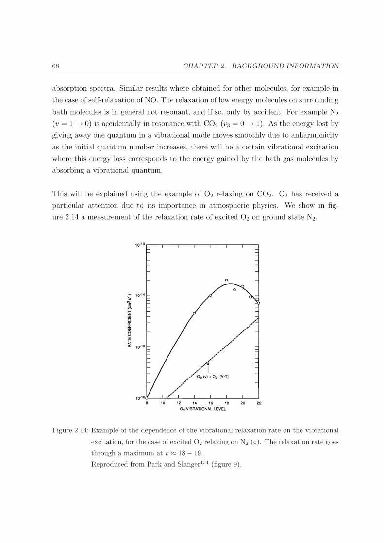
68 CHAPTER 2. BACKGROUND INFORMATION
absorption spectra. Similar results where obtained for other molecules, for example in
the case of self-relaxation of NO. The relaxation of low energy molecules on surrounding
bath molecules is in general not resonant, and if so, only by accident. For example N2
(v = 1 → 0) is accidentally in resonance with CO2 (v3 = 0 → 1). As the energy lost by
giving away one quantum in a vibrational mode moves smoothly due to anharmonicity
as the initial quantum number increases, there will be a certain vibrational excitation
where this energy loss corresponds to the energy gained by the bath gas molecules by
absorbing a vibrational quantum.
This will be explained using the example of O2 relaxing on CO2. O2 has received a
particular attention due to its importance in atmospheric physics. We show in fig-
ure 2.14 a measurement of the relaxation rate of excited O2 on ground state N2.
Figure 2.14: Example of the dependence of the vibrational relaxation rate on the vibrational
excitation, for the case of excited O2 relaxing on N2 (). The relaxation rate goes
through a maximum at v ≈ 18− 19.
Reproduced from Park and Slanger134 (figure 9).

2.3. COLLISIONAL VIBRATIONAL RELAXATION 69
Figure 2.14 shows a clear peak for v ≈ 18 − 19. This is because the energy mismatch
∆E for the process
O2(X3Σ−
g , v) + N2(0) → O2(X3Σ−
g , v − 2) + N2(1) + ∆E
goes through a minimum for this excitation level. This is an example of a 2-1 resonance,
but the principle is the same as for 1-1 resonances. Different functional dependencies
of the relaxation rates on the energy mismatch have been proposed and measured. For
example, in the case of relaxation of excited CO on ground state CO, a roughly gaussian
dependence has been observed135.
Other differences between low and highly excited molecules can be observed, for ex-
ample vibration to electronic (V-E) energy transfer or collision-induced dissociation
(for example NO2(v) + CO → NO + O + CO).
2.3.4 Isotopic influences on collisional relaxation
As we have pointed out in the previous section, the efficiency of vibrational energy
transfer depends largely on the energy mismatch of the emission and absorption of a
quantum in the two colliding molecules. We demonstrated this by the example of O2
relaxing on N2 (see figure 2.14). If the energy mismatch plays an important role for
the relaxation rates, one can expect that there should be some influences upon isotopic
substitution of an atom in one of the two colliding molecules, as this changes the vibra-
tional frequencies and hence the energy mismatch.
Isotopic influences on collisional relaxation rates have been observed as early as the
late 1960’s. For example, Stephenson, Wood and Moore112 reported isotopically selec-
tive relaxation rates for excited 12C16O2(0001) on ground state 12C16O18O and 13C16O2
(with roughly a factor of 2 between the relaxation rates) and on ground state 14N20
and 15N20 (with roughly a factor of 10 between the relaxation rates), which could be
explained by the different energy mismatches. Similarly, isotopically selective relaxation
of N2O on N2O136, CO on CO137 and CO on N2
138–141 has been found. We show in fig-
ure 2.15 a graph indicating different relaxation rates and their temperature dependence
for different isotopic partners for CO?-CO and CO?-N2 collisions (where the starred
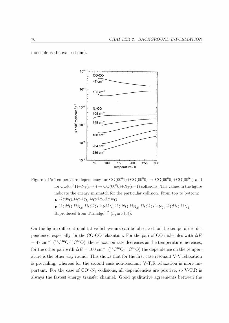
70 CHAPTER 2. BACKGROUND INFORMATION
molecule is the excited one).
Figure 2.15: Temperature dependency for CO(0001)+CO(0000) → CO(0000)+CO(0001) and
for CO(0001)+N2(v=0)→ CO(0000)+N2(v=1) collisions. The values in the figure
indicate the energy mismatch for the particular collision. From top to bottom:
I 12C16O-13C16O, 12C16O-13C18O.
I 12C16O-15N2, 12C16O-14N15N, 12C16O-14N2, 13C16O-14N2, 12C18O-14N2.
Reproduced from Turnidge137 (figure (3)).
On the figure different qualitative behaviours can be observed for the temperature de-
pendence, especially for the CO-CO relaxation. For the pair of CO molecules with ∆E
= 47 cm−1 (12C16O-13C16O), the relaxation rate decreases as the temperature increases,
for the other pair with ∆E = 100 cm−1 (12C16O-13C18O) the dependence on the temper-
ature is the other way round. This shows that for the first case resonant V-V relaxation
is prevailing, whereas for the second case non-resonant V-T,R relaxation is more im-
portant. For the case of CO?-N2 collisions, all dependencies are positive, so V-T,R is
always the fastest energy transfer channel. Good qualitative agreements between the
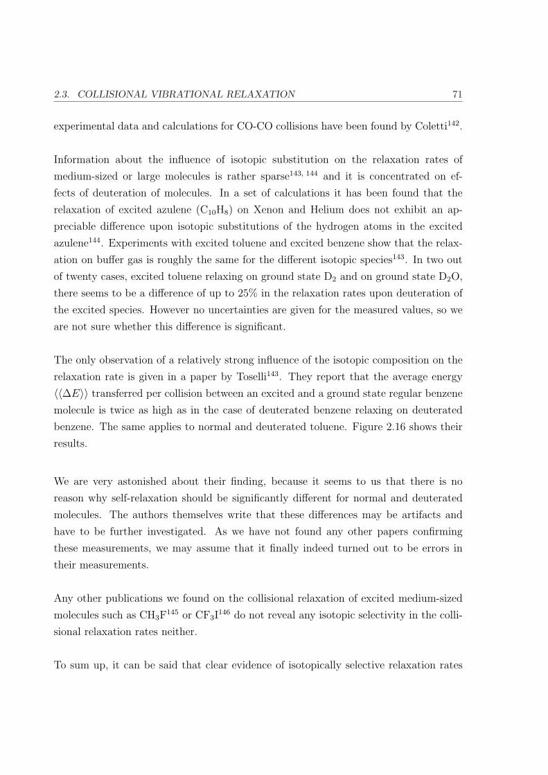
2.3. COLLISIONAL VIBRATIONAL RELAXATION 71
experimental data and calculations for CO-CO collisions have been found by Coletti142.
Information about the influence of isotopic substitution on the relaxation rates of
medium-sized or large molecules is rather sparse143, 144 and it is concentrated on ef-
fects of deuteration of molecules. In a set of calculations it has been found that the
relaxation of excited azulene (C10H8) on Xenon and Helium does not exhibit an ap-
preciable difference upon isotopic substitutions of the hydrogen atoms in the excited
azulene144. Experiments with excited toluene and excited benzene show that the relax-
ation on buffer gas is roughly the same for the different isotopic species143. In two out
of twenty cases, excited toluene relaxing on ground state D2 and on ground state D2O,
there seems to be a difference of up to 25% in the relaxation rates upon deuteration of
the excited species. However no uncertainties are given for the measured values, so we
are not sure whether this difference is significant.
The only observation of a relatively strong influence of the isotopic composition on the
relaxation rate is given in a paper by Toselli143. They report that the average energy
〈〈∆E〉〉 transferred per collision between an excited and a ground state regular benzene
molecule is twice as high as in the case of deuterated benzene relaxing on deuterated
benzene. The same applies to normal and deuterated toluene. Figure 2.16 shows their
results.
We are very astonished about their finding, because it seems to us that there is no
reason why self-relaxation should be significantly different for normal and deuterated
molecules. The authors themselves write that these differences may be artifacts and
have to be further investigated. As we have not found any other papers confirming
these measurements, we may assume that it finally indeed turned out to be errors in
their measurements.
Any other publications we found on the collisional relaxation of excited medium-sized
molecules such as CH3F145 or CF3I
146 do not reveal any isotopic selectivity in the colli-
sional relaxation rates neither.
To sum up, it can be said that clear evidence of isotopically selective relaxation rates
72 CHAPTER 2. BACKGROUND INFORMATION
Figure 2.16: Average energy 〈〈∆E〉〉 transferred between an excited molecule and the same
unexcited species.
Reproduced from Toselli143 (figure 1).
exists for small molecules (diatomics and triatomics), but from the literature it is not at
all clear that larger molecules should exhibit the same phenomenon. One would expect
little, if at all, isotopic influence on vibrational relaxation, because the density of vibra-
tional states of larger polyatomic molecules is very large and hence mixed. Because of
this extensive mixing, the donor and the acceptor molecules can always find a resonant
pathway for collisional vibrational energy transfer. We have not found any other works
on isotopically selective collisional relaxation of polyatomics since that publication in
1992.
Bibliography
[1] O. V. Boyarkin, M. Kowalczyk, and T. R. Rizzo. Collisionally Enhanced Isotopic
Selectivity in Multiphoton Dissociation of vibrationally excited CF3H . J. Chem.
Phys., 118(1):93–103, 2003.
[2] M. Lewerenz and M. Quack. Vibrational Overtone Intensities of the Isolated
CH and CD Chromophores in Fluoroform and Chloroform . Chem. Phys. Lett.,
BIBLIOGRAPHY 73
123(3):197–202, 1986.
[3] Robert McPheat and Geoffrey Duxbury. Infrared absorption cross-sections and
integrated absorption intensities of chloroform and fluoroform vapour . J. Quant.
Spectrosc. Rad. transf., 66:153–167, 2000.
[4] Andreas Amrein, Martin Quack, and Ulrich Schmitt. High resolution interfero-
metric Fourier transform infrared absorption spectroscopy in a supersonic free jet
expansion - The interacting states ν2, ν5 and ν3 + ν6 of trifluoromethane . Molec.
Phys., 60(1):237–248, 1987.
[5] H. J. Bernstein and G. Herzberg. Rotation-Vibration spectra of diatomic and
simple polyatomic molecules with long absorption paths. 1. The spectrum of Flu-
oroform (CHF3) from 2.5µ to 0.7µ . J. Chem. Phys., 16(1):30–39, 1948.
[6] R. A. Ashby. The infrared spectrum in the regions of the fundamentals of fluo-
roform . J. Molec. Spectrosc., 28(2):265–266, 1968.
[7] A. Ruoff, H. Burger, and S. Biedermann. Schwingungsspektren und Kraftkon-
stanten symmetrischer Kreisel - III Die IR-Spektren von HCF3 und DCF3 . Spec-
trochimica Acta, 27A:1359–1376, 1971.
[8] T. E. Sullivan and L. Frenkel. Measurement of fourth order distortion constants
in symmetric top molecules . J. Molec. Spectrosc., 39(2):185–201, 1971.
[9] P. Lockett and P. M. Wilt. Rotational Analysis of ν6 of DCF3 and ν3 + ν6 of
HCF3 . J. Chem. Phys., 60(8):3203–3207, 1974.
[10] N. J. Fyke, P. Lockett, J. K. Thompson, and P. M. Wilt. The Infrared Spectra
of HCF3 and DCF3 . J. Molec. Spectrosc., 58:87–101, 1975.
[11] H. F. Chambers, R. W. Kirk, J. K. Thompson, M. J. Warner, and P. M. Wilt.
The Infrared Spectrum of HC13F3 . J. Molec. Spectrosc., 58:76–86, 1975.
[12] R. W. Kirk and P. M. Wilt. General harmonic force-field of fluoroform . J. Molec.
Spectrosc., 58(1):102–110, 1975.
[13] C. E. Blom and A. Muller. A study on the GVFF of CHF3, CH2F2, and CH3F .
J. Molec. Spectrosc., 70(3):449–458, 1978.

74 CHAPTER 2. BACKGROUND INFORMATION
[14] G. Graner, R. Anttila, and J. Kauppinen. High-resolution infrared spectrum of
the ν3 and ν6 bands of HCF3 and of their hot bands . Mol. Phys., 38(1):103–128,
1979.
[15] Shigeo Kondo and Shinnosuke Saeki. Coriolis interactions and infrared intensities
in fluoroform . J. Chem. Phys., 74(12):6603–6611, 1981.
[16] Susumu Sofue, Kentarou Kawaguchi, Eizi Hirota, and Tsunetake Fujiyama. Ab-
solute Intensity Measurements of the ν4 Band of Fluoroform by the Use of a
Tunable Diode-laser Source . Bull. Chem. Soc. Jpn., 54:3546–3550, 1981.
[17] Hans-Rolf Dubal and Martin Quack. High-Resolution IR spectrum of Fluoroform:
A close Resonance . Chem. Phys. Lett., 80(3):439–444, 1981.
[18] G. Graner and G. Guelachvili. Fluoroform: the Polyad at 8-9 µm . J. Molec.
Spectrosc., 107:215–228, 1984.
[19] Robert C. Weast and Melvin J. Astle, editors. CRC Handbook of Chemistry and
Physics. CRC Press Inc., Florida, 59th edition, 1978.
[20] Hans-Rolf Dubal and Martin Quack. Tridiagonal Fermi resonance structure in
the IR spectrum of the excited CH chromophore in CF3H . J. Chem. Phys.,
81(9):3779–3791, 1984.
[21] Gunter Klatt, Andrew Willetts, Nicholas C. Handy, Riccardo Tarroni, and Paolo
Palmieri. An Improved Anharmonic Potential for CHF3 . J. Molec. Spectrosc.,
176:64–74, 1996.
[22] Enrico Fermi. Uber den Ramaneffekt des Kohlendioxyds . Z Phys, 71:250–259,
1931.
[23] Martin Quack. Spectra and Dynamics of coupled vibrations in polyatomic
molecules . Annu. Rev. Phys. Chem., 41:839–874, 1990.
[24] Gerhard Herzberg. Molecular Spectra and Molecular Structure. II. Infrared and
Raman Spectra of Polyatomic Molecules. Krieger Publishing Company: Malabar,
Florida, 1991.
BIBLIOGRAPHY 75
[25] J. Segall, R. N. Zare, H. R. Dubal, M. Lewerenz, and M. Quack. Tridiagonal
Fermi resonance structure in the IR spectrum of the excited CH chromophore in
CF3H . J. Chem. Phys., 86(2):634–646, 1987.
[26] Hans Hollenstein, Marius Lewerenz, and Martin Quack. Isotope effects in the
Fermi resonance of the CH Chromophore in CHX3 Molecules . Chem. Phys. Lett.,
165(2,3):175–183, 1990.
[27] A. S. Pine, G. T. Fraser, and J. M. Pliva. Molecular beam spectrum of the highly
perturbed C-H stretching region of fluoroform . J. Chem. Phys., 89(5):2720–2728,
1988.
[28] A. S. Pine and J. M. Pliva. Doppler-Limited Spectra of the C-H Bending Overtone
of Fluoroform . J. Molec. Spectrosc., 130:431–444, 1988.
[29] A. Amrein, M. Quack, and U. Schmitt. High-Resolution Interferometric Fourier-
Transform Infrared- Absorption Spectroscopy in Supersonic Free Jet Expan-
sions - Carbon-Monoxide, Nitric-Oxide, Methane, Ethyne, Propyne, and Trifluo-
romethane . J. Phys. Chem., 92(19):5455–5466, 1988.
[30] Zhen Lin, Kirk Boraas, and James P. Reilly. The vibrational overtone spectrum
of fluoroform in the ∆v=4 C-H stretching region . Chem. Phys. Lett., 217(3):239–
244, 1994.
[31] O. V. Boyarkin and T. R. Rizzo. Secondary time scales of intramolecular vibra-
tional energy redistribution in CF3H studied by vibrational overtone spectroscopy
. J. Chem. Phys., 105(15):6285–6292, 1996.
[32] O. V. Boyarkin, R. D. F. Settle, and T. R. Rizzo. Vibrational Overtone Spectra of
Jet-Cooled CF3H by Infrared Laser Assisted Photofragment Spectroscopy . Ber.
Bunsenges. Phys. Chem., 99(3):504–513, 1995.
[33] D. Romanini and A. Campargue. Vibrational overtone spectroscopy of the 41
band of CHF3 . Chem. Phys. Lett., 254:52–58, 1996.
[34] James S. Wong, William H. Green, Chi ke Cheng, and C. Bradley Moore. Cou-
pling of CH stretching and bending vibrations in trihalomethanes . J. Chem.
Phys., 86(11):5994–5999, 1987.
76 CHAPTER 2. BACKGROUND INFORMATION
[35] J. P. Champion and G. Graner. Fluoroform - A new analysis of the polyad at
8-9 µm . Molec. Phys., 58(3):475–484, 1986.
[36] David J. Nesbitt and Robert W. Field. Vibrational Energy Flow in Highly Excited
Molecules: Role of Intramolecular Vibrational Redistribution . J. Phys. Chem.,
100:12735–12756, 1996.
[37] K. K. Lehman, G. Scoles, and B. H. Pate. Intramolecular dynamics from
eigenstate-resolved infrared spectra . Annu. Rev. Phys. Chem., 45:241–274, 1994.
[38] John Keske and Brooks H. Pate. Decoding the Dynamical Information Embedded
in Highly Mixed Quantum States . Annu. Rev. Phys. Chem., 51:323–353, 2000.
[39] Izhack Oref and B. Seymour Rabinovitch. Do Highly Excited Reactive Polyatomic
Molecules Behave Ergodically ? . Acc. Chem. Res., 12:166–175, 1979.
[40] C. D. Cantrell. Multiple-Photon Excitation and Dissociation of Polyatomic
Molecules. Springer Verlag: Berlin Heidelberg New York, 1986.
[41] A. L. Malinovsky, E. A. Ryabov, and V. S. Letokhov. Laser time-resolved Raman
Spectroscopy of Mode Selectivity and Vibrational Energy Distribution for IR MP
Excited Polyatomic Molecules . Chem. Phys., 139:1989, 229-238.
[42] Christophe Iung, Fabien Gatti, and Hans-Dieter Meyer. Intramolecular vibra-
tional energy redistribution in the highly excited fluoroform molecule: A quantum
mechanical study using the multiconfiguration time-dependent Hartree algorithm
. J. Chem. Phys., 120(15):6992–6998, 2004.
[43] A. A. Kosterev, A. L. Malinovskii, and E. A. Ryabov. Fast vibrational relaxation
of valence vibrations of the C-H bond in halogenated methane . JETP Lett.,
54(1):14–17, 1991.
[44] A. A. Kosterev, A. L. Malinovsky, and E. A. Ryabov. Vibrational relaxation of
C-H stretching modes in methane and its halogenated derivatives . Chem. Phys.
Lett., 199(3,4):349–354, 1992.
[45] A. A. Kosterev, A. L. Malinovsky, and E. A. Ryabov. Ultrafast collisional redis-
tribution of vibrational energy in small polyatomic molecules . J. Molec. Struct.,
349:231–234, 1995.
BIBLIOGRAPHY 77
[46] A. A. Kosterev, A. L. Malinovsky, S. A. Tretyak, and E. A. Ryabov. Ultra-
fast Collisional Redistribution of Vibrational Energy in Highly Excited Poly-
atomic Molecules. The Role of Intramolecular Interactions . Ber. Bunsenges.
Phys. Chem., 99:378–380, 1995.
[47] J. T. Yardley. Introduction to Molecular Energy Transfer. Academic Press: New
York, 1980.
[48] Brian J. Orr. Collision-induced state-to-state energy transfer in perturbed rovi-
brational manifolds of small polyatomic molecules: mechanistic insights and ob-
servations. . Chem. Phys., 190:261–278, 1995.
[49] A. A. Kosterev, A. A. Makarov, A. L. Malinovsky, and E. A. Ryabov. Fast
collision-induced redistribution of vibrational energy in halogenated methanes .
Chem. Phys., 219:305–316, 1997.
[50] M. C. Borde, A. Henry, and M. L. Henry. Emission du gaz ammoniac excite par le
rayonnement d’un laser a gaz Carbonique . CR Acad. Sci. B Phys., 262(21):1389,
1966.
[51] M. C. Borde, A. Henry, and M. L. Henry. Comportement de differents gaz soumis
au rayonnement d’un laser a gaz Carbonique . CR Acad. Sci. B Phys., 263(9):619,
1967.
[52] N. V. Karlov, Y. N. Petrov, A. M. Prokhorov, and O. M. Atel’makh. Dissociation
of Boron Trichloride Molecules by CO2 Laser Radiation . JETP Lett., 11(4):135,
1970.
[53] W. B. Tiffany, H. W. Moos, and A. L. Schawlow. Selective Laser Photocatalysis
of Bromine Reactions . Science, 157:40–43, 1967.
[54] N. R. Isenor, V. Merchant, R. S. Hallsworth, and M. C. Richardson. CO2 laser
induced Dissociation of SiF4 Molecules into electronically excited fragments . Can.
J. Phys., 51(12):1281–1287, 1973.
[55] R. V. Ambartzumian, N. V. Chekalin, V. S. Doljikov, V. S. Letokhov, and E. A.
Ryabov. The Visible Luminescence Kinetics of BCl3 in the Field of a High-Power
CO2 Laser . Chem. Phys. Lett., 25(4):515–518, 1974.

78 CHAPTER 2. BACKGROUND INFORMATION
[56] V. S. Letokhov and A. A. Makarov. “Leakage” effect as an Exciting Mechanism
of High Vibrational Levels of Polyatomic Molecules by a Strong Quasi-Resonant
Laser IR Field . Optics Comm., 17(3):250–253, 1976.
[57] R. V. Ambartzumyan, V. S. Letokhov, E. A. Ryabov, and N. V. Chekalin. Isotopic
selective chemical reaction of BCl3 molecules in a strong infrared laser field . JETP
Lett., 20(9):273–274, 1974.
[58] Vladilen Stepanovic Letokhov. Laser spectroscopy of highly vibrationally excited
molecules. Adam Hilger, Bristol and Boston, 1989.
[59] M. G. Floquet. Sur les equations differentielles lineaires a coefficients periodiques
. Ann. Scient. Ecole Norm. Ser. 2, 12:47–XX, 1883.
[60] Martin Quack. Theory of unimolecular reactions induced by monochromatic
infrared radiation . J. Chem. Phys., 69(3):1282–1307, 1978.
[61] Martin Quack. Master Equations for Photochemistry with Intense Infrared Light
. Ber. Bunsenges. Phys. Chem., 83:757–775, 1979.
[62] Martin Quack. Master Equations for Photochemistry with Intense Infrared Light
(III) The Influence of Molecular Parameters in URIMIR . Ber. Bunsenges. Phys.
Chem., 83:1287–1293, 1979.
[63] Martin Quack. Master Equations for Photochemistry with Intense Infrared Light
(IV). A Unified Treatment of Case B and Case C Including Nonlinear Effects .
Ber. Bunsenges. Phys. Chem., 85:318–330, 1981.
[64] Martin Quack. Theory of Multiphoton Excitation . In Schleyer P. v. R.; Allinger
N. L.; Clark T.; Gasteiger J.; Kollman P. A.; Schaefer III H. F.; Schreiner P. R.,
editor, The Encyclopedia of Computational Chemistry. John Wiley & Sons, Chich-
ester, 1998.
[65] Martin Quack. Reaction Dynamics and statistical Mechanics of the preparation
of highly excited states by intense infrared Radiation . Adv. Chem. Phys., 50:396–
473, 1982.
[66] Martin Quack. Infrared laser Chemistry and the dynamics of molecular multi-
photon excitation . Infrared Phys., 29(2-4):441–466, 1989.
BIBLIOGRAPHY 79
[67] Martin Quack, Emile Sutcliffe, Peter A. Hackett, and David M. Rayner. Molecular
Photofragmentation with Many Infrared Photons . Faraday Discuss. Chem. Soc.,
82:229–240, 1986.
[68] M. Quack and E. Sutcliffe. On the validity of the quasiresonant approximation
for molecular infrared-multiphoton excitation . J. Chem. Phys., 83(8):3805–3812,
1985.
[69] Martin Quack. IR Laser Chemistry . Infrared Phys. and Technol., 36:365–380,
1995.
[70] Katharina von Puttkamer, Hans-Rolf Dubal, and Martin Quack. Time-dependent
Processes in Polyatomic Molecules During and After Intense Infrared Irradiation
. Faraday Discuss. Chem. Soc., 75:197–210, 1983.
[71] Donald W. Lupo and Martin Quack. IR-Laser Photochemistry . Chem. Rev.,
87:181–216, 1987.
[72] Martin Quack. Photochemistry with Infrared Radiation . Chimia, 35(12):463–
475, 1981.
[73] Vladilen Stepanovic Letokhov. Laser spectroscopy of highly vibrationally excited
molecules, chapter Chapter 1. Introduction to the Physics of Multiple-Photon Ex-
citation of Vibrations in Polyatomic molecules. Adam Hilger, Bristol and Boston;
ed. by V. S. Letokhov, 1989.
[74] O. V. Boyarkin, T. R. Rizzo, D. S. Rueda, M. Quack, and G. Seyfang. Nonlinear
intensity dependence in the infrared multiphoton excitation and dissociation of
methanol preexcited to different energies . J. Chem. Phys., 117(21):9793–9805,
2002.
[75] E. M. Alonso, J. A. O’Neill, and L. Pateopol. Non-linear processes in the IR
multiple-photon absorption of CF3H . J. Phys. B: At. Mol. Opt. Phys., 27:2217–
2227, 1994.
[76] J. A. O’Neill, L. Pateopol, and B. Pogue. Multiphoton absorption measurements
in CF3H . J. Phys. B: At. Mol. Opt. Phys., 25:3335–3344, 1992.
80 CHAPTER 2. BACKGROUND INFORMATION
[77] M. Quack and G. Seyfang. Frequency-dependent non-linear intensity dependence
in the IR Photochemistry of CF3I . Chem. Phys. Lett., 93(5):442–447, 1982.
[78] R. V. Ambartzumian, N. P. Furzikov, Y. A. Gorokhov, V. S. Lethokov, G. N.
Makarov, and A. A. Puretzky. Selective dissociation of SF6 molecules in a two-
frequency infrared laser field . Optics Commun., 18(4):517–521, 1976.
[79] J. D. Lambert. Vibrational and Rotational Relaxation in Gases. Oxford Clarendon
Press, 1977.
[80] A. B. Callear. Molecular Energy Transfer . Annu. Rep. Prog. Chem., 61:48–60,
1964.
[81] W. H. Flygare. Molecular Relaxation . Accounts Chem. Res., 1(4):121–127, 1968.
[82] D. C. Tardy and B. S. Rabinovitch. Intermolecular Vibrational Energy Transfer
in Thermal Unimolecular Systems . Chem. Rev., 77(3):369–408, 1977.
[83] I. Oref and D. C. Tardy. Energy Transfer in Highly Excited Large Polyatomic
Molecules . Chem. Rev., 90:1407–1445, 1990.
[84] Robert G. Gilbert. Theory of collisional energy transfer of highly excited
molecules . Int. Rev. Phys. Chem., 10(3):319–347, 1991.
[85] George W. Flynn, Charles S. Parmenter, and Alec M. Wodtke. Vibrational
Energy Transfer . J. Phys. Chem., 100:12817–12838, 1996.
[86] John R. Barker, Laurie M. Yoder, and Keith D. King. Vibrational Energy Transfer
Modeling of Nonequilibrium Polyatomic Reaction Systems . J. Phys. Chem. A,
105(5):796–809, 2001.
[87] Hai-Lung Dai. Highly Excited Molecules, chapter Collisional Energy Transfer of
Highly Vibrationally Excited Molecules: The Role of Long-Range Interaction and
Intramolecular Vibronic Coupling . ACS Symposium Series. American Chemical
Society, 1996.
[88] Ralph E. Weston and George W. Flynn. Relaxation of Molecules with Chemically
Significant Amounts of Vibrational Energy: The Dawn of the Quantum State
Resolved Era . Annu. Rev. Phys. Chem., 43:559–589, 1992.
BIBLIOGRAPHY 81
[89] Robert J. Gordon. Recent Trends in Experimental Studies of Vibrational Energy
Transfer . Comments At. Mol. Phys., 21(3):123–151, 1988.
[90] F. A. Lindemann, Svante Arrhenius, Irving Langmuir, N. R. Dhar, J. Perrin, and
W. C. McC. Lewis. Discussion on “the radiation theory of chemical action” .
Trans. Faraday Soc., 17:598–606, 1922.
[91] C. N. Hinshelwood. Quasi-Unimolecular Reactions. The Decomposition of Diethyl
Ether in the Gaseous State . Proc. Roy. Soc. London A, 114(766):84–97, 1927.
[92] C. N. Hinshelwood and P. J. Askey. Homogeneous Reactions Involving Complex
Molecules. The Kinetics of the Decomposition of Gaseous Dimethyl Ether . Proc.
Roy. Soc. London A, 114(770):215–226, 1927.
[93] C. N. Hinshelwood and P. J. Askey. The Influence of Hydrogen on Two Homo-
geneous Reactions . Proc. Roy. Soc. London A, 114(773):163–170, 1927.
[94] Oscar Knefler Rice and Herman C. Ramsperger. Theories of unimolecular gas
reactions at low Pressures . J. Am. Chem. Soc., 49(7):1617–1629, 1927.
[95] Oscar Knefler Rice. The Quantum Theory of Quasi-Unimolecular Gas Reactions
. Proc. Natl. Acad. Sci. U.S.A., 14(2):113–118, 1928.
[96] L. S. Kassel. Studies in Homogeneous Gas Reactions. II. Introduction of Quantum
Theory . J. Phys. Chem., 32(7):1065–1079, 1928.
[97] A. B. Callear. Vibrational relaxation of Nitric Oxide . Discuss. Faraday Soc.,
33:33–36, 1962.
[98] G. Hancock and I. W. M. Smith. Quenching of infrared chemiluminescence. 1.
Rates of de-excitation of CO(4 ≤ v ≤ 13) by He, CO, NO, N2, O2, OCS, N2O,
and CO2 . Appl. Opt., 10(8):1827–1842, 1971.
[99] C. Wittig and I. W. M. Smith. Vibrational energy transfer in carbon monoxide
at low temperatures . J. Chem. Soc. - Faraday Trans. 2, 69:939–951, 1973.
[100] R. N. Schwartz, Z. I. Slawsky, and K. F. Herzfeld. Calculation of Vibrational
Relaxation Times in Gases . J. Chem. Phys., 20(10):1591–1599, 1952.

82 CHAPTER 2. BACKGROUND INFORMATION
[101] W. A. Rosser, A. D. Wood, and E. T. Gerry. Deactivation of Vibrationally
Excited Carbon Dioxide (ν3) by Collisions with Carbon Dioxide or with Nitrogen
. J. Chem. Phys., 50(11):4996–5008, 1969.
[102] Bruce H. Mahan. Resonant Transfer of Vibrational Energy in Molecular Collisions
. J. Chem. Phys., 46(1):98–101, 1967.
[103] T. A. Dillon and J. C. Stephenson. Multiquantum Vibrational-Energy Exchange
. Phys. Rev. A, 6(4):1460–1468, 1972.
[104] Donald Rapp and Thomas Kassal. The theory of vibrational energy transfer
between simple molecules in nonreactive collisions . Chem. Rev., 69:61–102, 1968.
[105] Frank I. Tanczos. Calculation of Vibrational Relaxation Times of the
Chloromethanes . J. Chem. Phys., 25(3):439–447, 1956.
[106] L. D. Landau and E. M. Lifschitz. Quantum mechanics: non-relativistic theory.
London; Pergamon Press, 1958.
[107] S. Califano. Vibrational States. John Wiley and Sons, 1976.
[108] John C. Stephenson and C. Bradley Moore. Near-Resonant Vibration → Vibra-
tion Energy Transfer: CO2 (ν3=1) + M → CO2 (ν1 = 1) + M? + ∆E . J. Chem.
Phys., 52(5):2333–2340, 1970.
[109] R. D. Sharma and C. A. Brau. Near-Resonant vibrational energy transfer in
N2-CO2 Mixtures . Phys. Rev. Lett., 19(22):1273–1275, 1967.
[110] R. D. Sharma and C. A. Brau. Energy Transfer in Near-Resonant Molecular
Collisions due to Long-Range Forces with Application to Transfer of Vibrational
Energy from ν3 Mode of CO2 to N2 . J. Chem. Phys., 50(2):924–930, 1969.
[111] R. D. Sharma. Vibration-to-Vibration energy transfer in CO-CO collisions .
Chem. Phys. Lett., 30(2):261–266, 1975.
[112] John C. Stephenson, Robert E. Wood, and C. Bradley Moore. Near-Resonant
Energy Transfer between Infrared-Active Vibrations . J. Chem. Phys., 48:4790–
4791, 1968.
BIBLIOGRAPHY 83
[113] R. D. Sharma. Near-Resonant Vibrational Energy Transfer Among Isotopes of
CO2 . Phys. Rev., 177(1):102–107, 1969.
[114] T. A. Dillon and J. C. Stephenson. Effect of the straight path approximation and
exchange forces on vibrational energy transfer . J. Chem. Phys., 58(9):3849–3854,
1973.
[115] T. A. Dillon and J. C. Stephenson. Calculation of vibrational and rotational
energy transfer between HF, DF, HCl, and CO2 . J. Chem. Phys., 58(5):2056–
2064, 1973.
[116] V. T. Platonenko and N. A. Sukhareva. On vibrational energy exchange between
strongly excited polyatomic molecules . Sov. Phys. JETP, 51(6):1065–1071, 1980.
[117] V. T. Platonenko and N. A. Sukhareva. Vibrational relaxation of strongly excited
polyatomic molecules . Sov. Phys. JETP, 54(3):454–459, 1981.
[118] V. M. Akulin. Singularities of collisional vibrational relaxation processes in
strongly excited spectrally complex polyatomic molecules . Sov. Phys. JETP,
57(4):774–780, 1983.
[119] Raymond L. Taylor and Steven Bitterman. Experimental Measurements of the
Resonant Vibrational Energy Transfer between Mode ν3 of CO2 and N2 . J. Chem.
Phys., 50(4):1720–1726, 1969.
[120] R. G. Gilbert. Collisional Energy Transfer Exchange in Highly Vibrationally Ex-
cited Molecules - the Biased Random Walk Model . J. Chem. Phys., 80(11):5501–
5509, 1984.
[121] M. Quack and J. Troe. Unimolecular reactions and energy transfer of highly
excited molecules. In P.G. Ashmore and R.J. Donovan, editors, Gas Kinetics and
Energy Transfer 2. The Chemical Society London, 1977.
[122] B. Abel, B. Herzog, H. Hippler, and J. Troe. Infrared multiphoton excitation
of CF3I. II. Collisional energy transfer of vibrationally highly excited CF3I . J.
Chem. Phys., 91(2):900–905, 1989.
[123] Uwe Hold, Thomas Lenzer, Klaus Luther, and Andrew C. Symonds. Collisional
energy transfer probabilities of highly excited molecules from KCSI. III. Azulene:
84 CHAPTER 2. BACKGROUND INFORMATION
P (E ′, E) and moments of energy transfer for energies up to 40 000 cm−1 via
self-calibrating experiments . J. Chem. Phys., 119(21):11192–11211, 2003.
[124] Arthur J. Sedlacek, Ralph E. Weston, and George W. Flynn. Interrogating the
vibrational-relaxation of highly excited polyatomics with time-resolved diode-laser
spectroscopy - C6H6, C6D6 and C6F6 + CO2 . J. Chem. Phys., 94(10):6483–6490,
1991.
[125] C. P. Bewick, J. F. Martins, and B. J. Orr. Rotationally specific mode-to-mode
vibrational energy transfer in D2CO/D2CO collisions. II. Kinetics and modelling
. J. Chem. Phys., 93(2):8643–8657, 1990.
[126] S. Hassoon, I. Oref, and C. Steel. Collisional activation of quadricyclane by
azulene - an example of very strong Collisions . J. Chem. Phys., 89(3):1743–1744,
1988.
[127] F. F. Crim. Selective Excitation Studies of Unimolecular Reaction Dynamics .
Annu. Rev. Phys. Chem., 35:657–691, 1984.
[128] C. E. Hamilton, J. L. Kinsey, and R. W. Field. Stimulated Emission Pumping:
New Methods in Spectroscopy and Molecular Dynamics . Annu. Rev. Phys. Chem.,
37:493–524, 1986.
[129] R. N. Schwartz and K. F. Herzfeld. Vibrational relaxation times in gases (3-
dimensional treatment) . J. Chem. Phys., 22(5):767–773, 1954.
[130] C. A. Rogaski, J. A. Mack, and A. M. Wodtke. State-to-state Rate Constants
for Relaxation of Highly Vibrationally Excited O2 and Implications for its Atmo-
spheric Fate . Faraday Discuss., 100:229–251, 1995.
[131] J. A. Mack, K. Mikulecky, and A. M. Wodtke. Resonant vibration-vibration
energy transfer between highly vibrationally excited O2(X3Σ−
g , v = 15 - 26) and
CO2, N2, N2 and O3 . J. Chem. Phys., 105(10):4105–4116, 1996.
[132] M. L. Nowlin and M. C. Heaven. Energy transfer rate constants for highly excited
rovibrational levels of I2(X) . J. Chem. Phys., 99(8):5654–5660, 1993.
[133] X. Yang, J. M. Price, J. A. Mack, C. G. Morgan, C. A. Rogaski, D. McGuire,
E. H. Kim, , and A. M. Wodtke. Stimulated emission pumping studies of energy
BIBLIOGRAPHY 85
transfer in highly vibrationally excited molecules . J. Phys. Chem., 97(16):3944–
3955, 1993.
[134] H. Park and T. G. Slanger. O2(X, v = 8−22) 300 K quenching rate coefficients of
O2 and N2, and O2(x) vibrational distribution from 248 nm O3 photodissociation
. J. Chem. Phys., 100(1):287–300, 1994.
[135] H. T. Powell. Vibrational relaxation of carbon monoxide using a pulse discharge.
II. T = 100, 300, 500 K . J. Chem. Phys., 63(6):2635–2645, 1975.
[136] L. Doyennette, M. Margottin-Maclou, A. Chakroun, H. Gueguen, , and L. Henry.
Vibrational energy transfer from the (0001) level of 14N2O and 12CO2 to the (m,
nl, 1) levels of these molecules and of their isotopic species . J. Chem. Phys.,
62(2):440–447, 1975.
[137] M. L. Turnidge, J. P. Reid, P. W. Barnes, and C. J. S. M. Simpson. Vibrational
energy transfer between the isotopomers of carbon monoxide at low temperatures
. J. Chem. Phys., 108(2):485–491, 1998.
[138] D. C. Allen and C. J. S. M. Simpson. Vibrational energy exchange between CO
and the isotopes of N2 between 300 K and 80 K . Chem. Phys., 45(2):171–334,
1980.
[139] E. T. Chandler, E. A. Gregory, R. M. Siddles, and C. J. S. M. Simpson. Vi-
brational energy exchange between CO(v=1) and 14N2 and CO(v=1) and 15N2
measured to 60 K in the gas phase . Chem. Phys. Lett., 78(2):236–240, 1981.
[140] H. T. Williams, S. V. Gwynne, and C. J. S. M. Simpson. Non-and near-resonant
(VV) energy transfer between the isotopes of N2 and of CO in liquid Ar and in
the gas phase at 85 K . Chem. Phys. Lett., 138(1):95–98, 1987.
[141] G. J. Wilson, M. L. Turnidge, and C. J. S. M. Simpson. Vibrational energy
transfer between 12C16O and 15N2 in the gas phase down to 45 K and in liquid Ne
solution . Chem. Phys. Lett., 227(3):299–304, 1994.
[142] Cecilia Coletti and Gert D. Billing. Isotopic effects on vibrational energy transfer
in CO . J. Chem. Phys., 111(9):3891–3897, 1999.
86 CHAPTER 2. BACKGROUND INFORMATION
[143] Beatriz M. Toselli and John R. Barker. Isotope effects in the vibrational deacti-
vation of large molecules . J. Chem. Phys., 97(3):1809–1817, 1992.
[144] David L. Clarke and Robert G. Gilbert. Collisional Energy Transfer in Highly
Excited Molecules: Deuteration effects . J. Phys. Chem., 96:8450–8453, 1992.
[145] Jack M. Preses and George W. Flynn. Infrared laser double resonance study
of vibrational energy exchange between 12CH3F and 13CH3F? . J. Chem. Phys.,
66(7):3112–3116, 1977.
[146] Martin Quack, Rene Schwarz, and Georg Seyfang. Time-resolved infrared-
spectroscopic observation of relaxation and reaction processes during and after
infrared-multiphoton excitation of 12CF3I and 13CF3I with shaped nanosecond
pulses . J. Chem. Phys., 96(12):8727–8740, 1992.

Chapter 3
Experimental setup
In this chapter we present our experimental setup. In the first part, in section 3.1,
we present the optical setup, in section 3.2 we discuss the ideal sample pressure for
our experiments, and in section 3.3 we present the chemical synthesis of isotopically
enriched CF3H used in our experiments.
3.1 Optical setup of our experiments
In this section we present the optical setup of our experiments. First, in the sub-
section 3.1.1, we recall the general energy level diagram followed in our experiments.
Then, the sub-section 3.1.2 describes optical setup in details. After that, the sub-
sections 3.1.3-3.1.5 describe how the laser radiation is generated for pre-excitation of
the CF3H molecules via the different overtones of the CH stretching bending vibration.
Finally, the sub-section 3.1.6 describes how we determine the fluence of the second laser,
which is a critical value in our experimental investigations.
3.1.1 General energy level diagram
We have previously described the proposed setup for the new laser isotope separation
process which consists of selectively dissociating vibrationally pre-excited molecules
(section 1.1). For the investigation of the mechanisms leading to an increase of iso-
topic selectivity upon increasing the sample pressure or the time-delay between the
two lasers, we need to detect the photofragments. This can be done, for example, by
87

88 CHAPTER 3. EXPERIMENTAL SETUP
mass-spectrometric detection of the products of the MLIS procedure after recombina-
tion via CF2 + CF2 → C2F4. An alternative way is to detect the CF2 fragments in
situ via LIF before recombination. In this work we chose this latter detection method,
as this allows us to monitor the number of dissociated CF3H molecules in real time.
Because we use LIF for the detection of the fragments, our experimental procedure
resembles very much to the one we would use to record absorption spectra using the IR-
LAPS method. We show in figure 3.1 a general energy level diagram of our experiments.
Figure 3.1: General energy level diagram used in our experiments.
First, a laser pulse pre-excites room temperature CF3H molecules through a vibra-
tional overtone transition of the CH stretching-bending vibration. Following this,
a pulse from a tunable TEA CO2 laser promotes some fraction of the vibrationally
excited molecules to energies above their dissociation limit by infrared multiple
photon excitation (IRMPE). We monitor CF2 fragments by a third laser pulse via
laser induced fluorescence (LIF).

3.1. OPTICAL SETUP OF OUR EXPERIMENTS 89
Although LIF is, at least in principle, isotopically selective, in the case of CF2 the elec-
tronic transitions are broadened and substantially overlapped, such that, in practice,
isotopically selective LIF is impossible (for the CF2 fragments we estimate a shift of ∼1
cm−1 between the transitions of the two isotopic species1, which has to be compared
with a typical width of ∼50 cm−1 of a single absorption feature2). Our measured LIF
signals are both due to dissociated 12CF3H and 13CF3H, and we correct them adequately
in our data analysis‡.
Excited CF2 can also relax via non-radiative energy transfer in collisions, so the mea-
sured LIF signal is not necessarily proportional to the number of dissociated CF3H
molecules. This effect, collisional quenching, is also taken into account in our data anal-
ysis. We show in appendix B the effect of collisional quenching of excited CF2 and how
the results are corrected.
3.1.2 General optical setup
Figure 3.2 shows the main features of the optical layout in our experimental setup.
The generation of the light for the pre-excitation of the molecules depends on the pre-
excitation level. We will describe the different methods in the following sections.
For the IRMPD step, we use a 10 µm pulse from a line tunable TEA CO2 laser (Lumon-
ics, TEA-840, bandwidth ∼0.1-0.15 cm−1) that consists of an intense 250 ns (FWHM)
spike and a 5-10 µs low intensity tail. The first spike contains ∼30-40 % of the total
pulse energy. A TEM00 laser beam is produced by inserting a 10 mm iris into the CO2
laser cavity. The total energy of a typical laser pulse is up to 300 mJ. The laser light is
focussed by a 70 cm ZnS lens into the cell. Before entering the cell, the CO2 laser light
can be attenuated by a set of teflon sheets.
‡In the case of natural abundant gas (∼ 99% 12CF3H), we first measure the decay rate for pre-excited12CF3H; the signal contains no contribution of pre-excited 13CF3H. By taking an IRLAPS excitation spectrum
around the Q-branch of 13CF3H, we determine the dissociation selectivity at a zero time-delay (see for example
section 4.3.3). With these pieces of information the contributions due to excited 12CF3H and due to excited13CF3H for the case of pre-excitation at the Q-branch of 13CF3H is easily calculated. Similar considerations
apply to carbon-13 enriched samples.

90 CHAPTER 3. EXPERIMENTAL SETUP
Figure 3.2: Optical setup of the experiments.
LS = laser for the pre-excitation of the molecules. L1: Nd:YAG pumped dye laser,
L2: TEA CO2 laser. PB = Pellin-Broca prism. SHG = autotracker for second
harmonic generation. Det1...3 = detectors. HR = highly reflective mirror for UV
light. F: filter for visible light. Sh = mechanical shutter. PH = pinhole. Sa =
Sapphire plate. BaF2 = windows. C = cell. PA = photoacoustic cell. T = teflon
sheets.
The experiments are performed at a rate of 10 Hz.
For LIF detection of CF2 we use the 5-10 mJ output of a Nd:YAG pumped (Lumonics,
YM 600) dye laser (Continuum, ND60, linewidth ∼0.08 cm−1, Coumarin-500 dye) that
has been frequency-doubled in a BBO crystal. The remaining green light after frequency
doubling is separated out by a UG-5 filter (Schott). Some green light is reflected on
the front surface of the filter and directed into a beamstopper. The laser wavelength
is tuned to the A(0, 2, 0)1B1 ← X(0, 1, 0)1A1 electronic transition3 in CF2 at ∼266.08
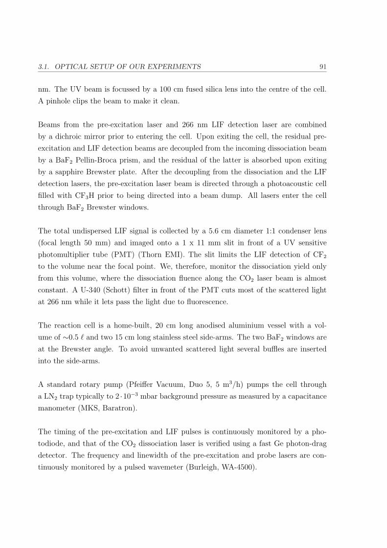
3.1. OPTICAL SETUP OF OUR EXPERIMENTS 91
nm. The UV beam is focussed by a 100 cm fused silica lens into the centre of the cell.
A pinhole clips the beam to make it clean.
Beams from the pre-excitation laser and 266 nm LIF detection laser are combined
by a dichroic mirror prior to entering the cell. Upon exiting the cell, the residual pre-
excitation and LIF detection beams are decoupled from the incoming dissociation beam
by a BaF2 Pellin-Broca prism, and the residual of the latter is absorbed upon exiting
by a sapphire Brewster plate. After the decoupling from the dissociation and the LIF
detection lasers, the pre-excitation laser beam is directed through a photoacoustic cell
filled with CF3H prior to being directed into a beam dump. All lasers enter the cell
through BaF2 Brewster windows.
The total undispersed LIF signal is collected by a 5.6 cm diameter 1:1 condenser lens
(focal length 50 mm) and imaged onto a 1 x 11 mm slit in front of a UV sensitive
photomultiplier tube (PMT) (Thorn EMI). The slit limits the LIF detection of CF2
to the volume near the focal point. We, therefore, monitor the dissociation yield only
from this volume, where the dissociation fluence along the CO2 laser beam is almost
constant. A U-340 (Schott) filter in front of the PMT cuts most of the scattered light
at 266 nm while it lets pass the light due to fluorescence.
The reaction cell is a home-built, 20 cm long anodised aluminium vessel with a vol-
ume of ∼0.5 ` and two 15 cm long stainless steel side-arms. The two BaF2 windows are
at the Brewster angle. To avoid unwanted scattered light several buffles are inserted
into the side-arms.
A standard rotary pump (Pfeiffer Vacuum, Duo 5, 5 m3/h) pumps the cell through
a LN2 trap typically to 2 ·10−3 mbar background pressure as measured by a capacitance
manometer (MKS, Baratron).
The timing of the pre-excitation and LIF pulses is continuously monitored by a pho-
todiode, and that of the CO2 dissociation laser is verified using a fast Ge photon-drag
detector. The frequency and linewidth of the pre-excitation and probe lasers are con-
tinuously monitored by a pulsed wavemeter (Burleigh, WA-4500).

92 CHAPTER 3. EXPERIMENTAL SETUP
To ensure stable experimental conditions and correct the LIF signal, we continuously
monitor the relative power of the lasers during the course of an experiment by photo-
diodes that detect reflections from the entrance windows. As the CO2 laser displays in
general a rather stable intensity (after some warming up time), normally only the LIF
and the pre-excitation laser beams are monitored.
Our measurements are not background free, since some dissociated ground state molecules
and scattered light can also contribute to the measured signal. Every measured value
is obtained by first measuring the collected LIF signal as described above and then
by measuring the same signal by blocking the pre-excitation laser with a mechanical
shutter. The difference of the two signals is proportional to the amount of dissociated
pre-excited molecules.
The lasers and the signals are timed as follows: ∆tPE−IRMPD is the time-delay be-
tween the pre-excitation (PE) laser pulse and the onset of the CO2 (IRMPD) laser
pulse (see figure 3.3). ∆tIRMPD−LIF is the time-delay between the CO2 and the LIF
(UV) laser pulses. It is typically kept to 800 ns.

3.1. OPTICAL SETUP OF OUR EXPERIMENTS 93
Inte
nsity
[a.u
.]
12008004000Time [ns]
∆tPE-IRMPD ∆tIRMPD-UV
(in general 800 ns)
Pre-excitation laser (PE)LIF laser (UV)
CO2 laser (IRMPD)
Figure 3.3: Timing of pre-excitation, dissociation and LIF lasers. Here an example for a time-
delay of 600 ns between pre-excitation and dissociation lasers.
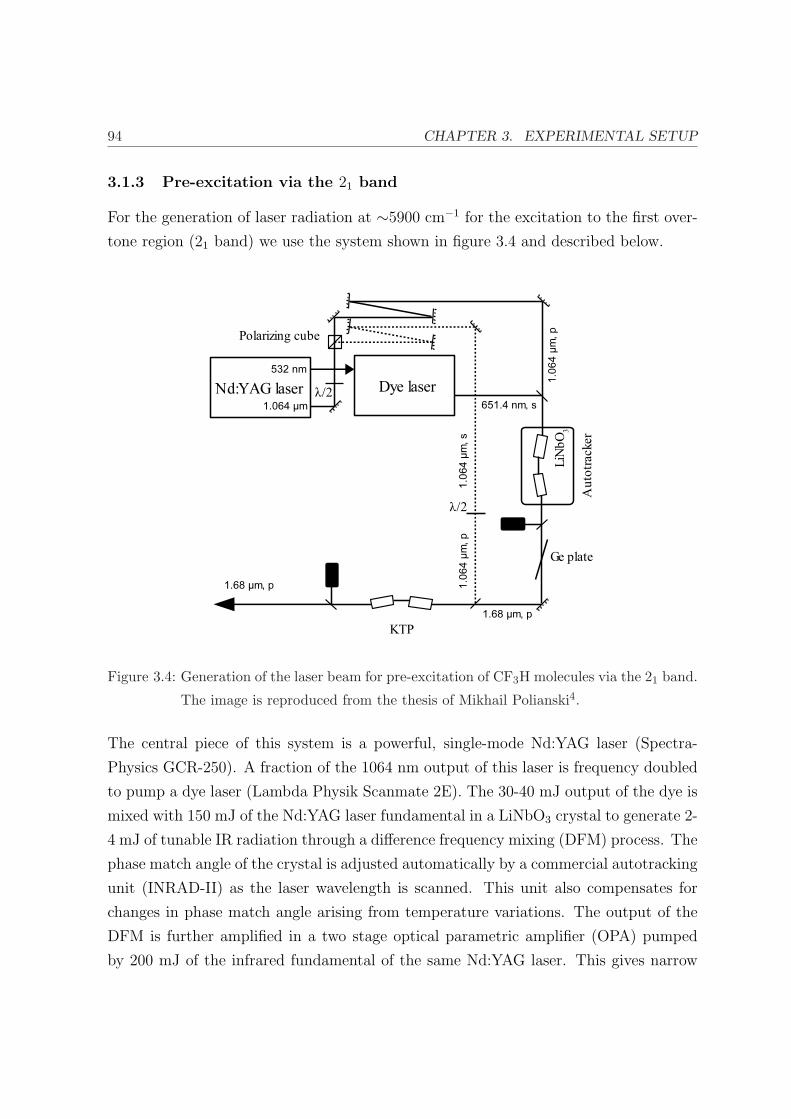
94 CHAPTER 3. EXPERIMENTAL SETUP
3.1.3 Pre-excitation via the 21 band
For the generation of laser radiation at ∼5900 cm−1 for the excitation to the first over-
tone region (21 band) we use the system shown in figure 3.4 and described below.
Figure 3.4: Generation of the laser beam for pre-excitation of CF3H molecules via the 21 band.
The image is reproduced from the thesis of Mikhail Polianski4.
The central piece of this system is a powerful, single-mode Nd:YAG laser (Spectra-
Physics GCR-250). A fraction of the 1064 nm output of this laser is frequency doubled
to pump a dye laser (Lambda Physik Scanmate 2E). The 30-40 mJ output of the dye is
mixed with 150 mJ of the Nd:YAG laser fundamental in a LiNbO3 crystal to generate 2-
4 mJ of tunable IR radiation through a difference frequency mixing (DFM) process. The
phase match angle of the crystal is adjusted automatically by a commercial autotracking
unit (INRAD-II) as the laser wavelength is scanned. This unit also compensates for
changes in phase match angle arising from temperature variations. The output of the
DFM is further amplified in a two stage optical parametric amplifier (OPA) pumped
by 200 mJ of the infrared fundamental of the same Nd:YAG laser. This gives narrow
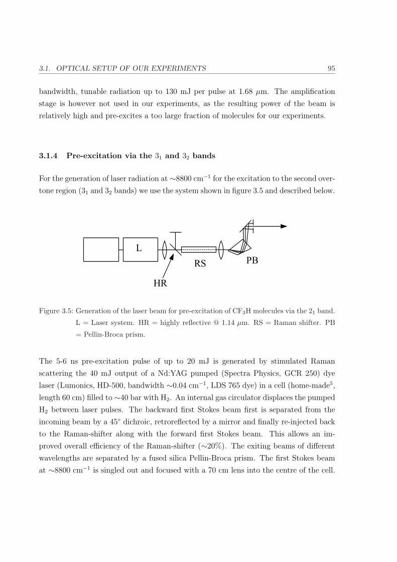
3.1. OPTICAL SETUP OF OUR EXPERIMENTS 95
bandwidth, tunable radiation up to 130 mJ per pulse at 1.68 µm. The amplification
stage is however not used in our experiments, as the resulting power of the beam is
relatively high and pre-excites a too large fraction of molecules for our experiments.
3.1.4 Pre-excitation via the 31 and 32 bands
For the generation of laser radiation at ∼8800 cm−1 for the excitation to the second over-
tone region (31 and 32 bands) we use the system shown in figure 3.5 and described below.
Figure 3.5: Generation of the laser beam for pre-excitation of CF3H molecules via the 21 band.
L = Laser system. HR = highly reflective @ 1.14 µm. RS = Raman shifter. PB
= Pellin-Broca prism.
The 5-6 ns pre-excitation pulse of up to 20 mJ is generated by stimulated Raman
scattering the 40 mJ output of a Nd:YAG pumped (Spectra Physics, GCR 250) dye
laser (Lumonics, HD-500, bandwidth ∼0.04 cm−1, LDS 765 dye) in a cell (home-made5,
length 60 cm) filled to ∼40 bar with H2. An internal gas circulator displaces the pumped
H2 between laser pulses. The backward first Stokes beam first is separated from the
incoming beam by a 45 dichroic, retroreflected by a mirror and finally re-injected back
to the Raman-shifter along with the forward first Stokes beam. This allows an im-
proved overall efficiency of the Raman-shifter (∼20%). The exiting beams of different
wavelengths are separated by a fused silica Pellin-Broca prism. The first Stokes beam
at ∼8800 cm−1 is singled out and focused with a 70 cm lens into the centre of the cell.

96 CHAPTER 3. EXPERIMENTAL SETUP
3.1.5 Pre-excitation via the 41 and 52 bands
For the pre-excitation of the molecules in the 11,600 and in the 14,000 cm−1 regions (pre-
excitation via the 41 and 52 bands), we directly use the output of a Nd:YAG pumped
dye laser.
3.1.6 Control of the fluence of the dissociation laser
The dissociation process with the second laser depends non-linearly on the fluence of
this laser beam. Unfortunately, the power of the CO2 laser beam can only be adjusted
over as small range without changing the focal properties of the laser beam. We chose
to attenuate the beam with a set of 0.1 mm thick teflon sheets. The fluence is calculated
as follows:
Φ =E · f1 · f2 · exp (−εn)
πr20
, (3.1)
where E is the energy in the whole pulse, f1 is the fraction of transmitted light from
where we measure the power at the centre of the cell, f2 is the temporal fraction of the
pulse used, ε is an absorption parameter of teflon, n is the number of sheets used for
the attenuation and r0 is the radius of the laser beam in the centre of the cell. With
this system, the fluence can be adjusted over a large range of energies (however not
continuously) without changing the focussing properties of the laser beam. We give
some details in appendix C.
3.2 Working pressure
In some experiments we wish to work at low pressures in order to avoid collisional
relaxation during IRMPD. This way, an increase of isotopic selectivity can be well
separated into isotopically selective collisional relaxation and different IRMPD rates.
However, two effects limit the pressure towards the bottom:
1. Molecules flying out of the reaction volume: If we pre-excite a certain
amount of molecules at t = 0, we want to be sure that the molecules are still in
the reaction volume after a time-delay of ∆t on the time-scales of our experiments

3.2. WORKING PRESSURE 97
(typically hundreds of ns to a couple of µs). By measuring some pressure depen-
dent decay rates we determine that for a pressure of & 1 mbar it is safe to assume
no losses of molecules this way. Figure 3.6 shows the decay rate k (the loss of
dissociated molecules as the time-delay between the laser pulses is increased) as
a function of the pressure p. The measurements are taken for 13CF3H molecules
pre-excited via the 31 band at a moderate CO2 laser fluence.
4x10⁻³
3
2
1
0
k [n
s-1 m
bar-1
]
0.12 3 4 5 6
12 3 4 5 6
102
pressure [mbar]
Figure 3.6: The decay rate k goes up as p goes down, indicating that molecules flying out of
the reaction volume falsify the experimental measurement.
For pressures . 1 mbar the fly-out gets important.
2. Rotational relaxation: The data analysis is highly facilitated if we can always
assume complete rotational relaxation of the molecules, thus avoiding a rotational
bottleneck in IRMPD. In order to investigate on this, we measure the IRMPD
yield as a function of the pressure for molecules pre-excited via the 21 band. In
figure 3.7-a the dissociation yield Y is plotted for pressures between 0 and 2 mbar.
The measured data can be fitted by an empirical function

98 CHAPTER 3. EXPERIMENTAL SETUP
500
400
300
200
100
0
Y [a
.u.]
2.01.51.00.50.0
Pressure [mbar]
(a) Dissociation yield Y as a function of the
pressure p.
80
60
40
20
0
Y [a
.u.]
0.300.200.100.00
Pressure [mbar]
(b) Blowup of figure (a).
Figure 3.7: Measurements for rotational relaxation. At low pressures the relative dissociation
yield goes down. The solid curve represents a phenomenological fit and the dotted
line would be the yield if rotational relaxation were complete. All measurements
are for 12CF3H. The results are corrected for quenching.
Y (p) = η · p ·(
1− exp
(−p
%
))2
, (3.2)
where η and % are fitting constants, η incorporates all transmission efficiencies and
conversion constants and p is the sample pressure. % has been found to be ∼ 0.27
mbar. The value of % depends on the exact experimental conditions such as e.g.
dissociation laser fluence, but it can be used as indicative value. We define the
value ε to be the “completeness of rotational relaxation”, where
ε =
(1− exp
(−p
%
))2
. (3.3)
It is plotted in figure 3.8. It can be seen that for pressures of p & 1 mbar rotational
relaxation can be considered to be complete for pre-excitation via the 21 band.
For these reasons, the measurements with time-delayed laser pulses are performed at a
pressure of 1 mbar.
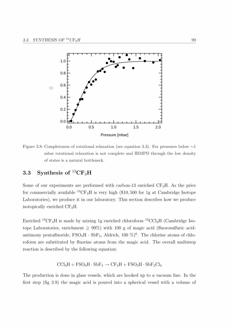
3.3. SYNTHESIS OF 13CF3H 99
1.0
0.8
0.6
0.4
0.2
0.0
∈
2.01.51.00.50.0
Pressure [mbar]
Figure 3.8: Completeness of rotational relaxation (see equation 3.3). For pressures below ∼1
mbar rotational relaxation is not complete and IRMPD through the low density
of states is a natural bottleneck.
3.3 Synthesis of 13CF3H
Some of our experiments are performed with carbon-13 enriched CF3H. As the price
for commercially available 13CF3H is very high ($10, 500 for 1g at Cambridge Isotope
Laboratories), we produce it in our laboratory. This section describes how we produce
isotopically enriched CF3H.
Enriched 13CF3H is made by mixing 1g enriched chloroform 13CCl3H (Cambridge Iso-
tope Laboratories, enrichment ≥ 99%) with 100 g of magic acid (fluorosulfuric acid-
antimony pentafluoride, FSO3H · SbF5, Aldrich, 100 %)6. The chlorine atoms of chlo-
roform are substituted by fluorine atoms from the magic acid. The overall multistep
reaction is described by the following equation:
CCl3H + FSO3H · SbF5 → CF3H + FSO3H · SbF2Cl3
The production is done in glass vessels, which are hooked up to a vacuum line. In the
first step (fig 3.9) the magic acid is poured into a spherical vessel with a volume of
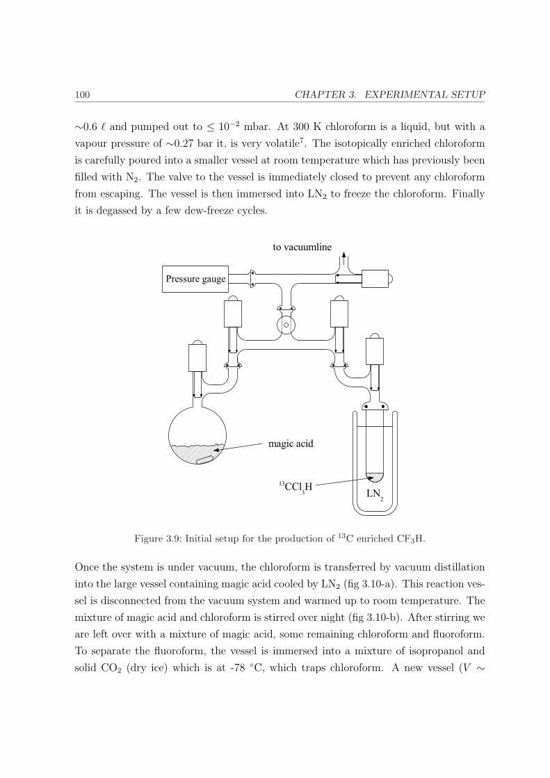
100 CHAPTER 3. EXPERIMENTAL SETUP
∼0.6 ` and pumped out to ≤ 10−2 mbar. At 300 K chloroform is a liquid, but with a
vapour pressure of ∼0.27 bar it, is very volatile7. The isotopically enriched chloroform
is carefully poured into a smaller vessel at room temperature which has previously been
filled with N2. The valve to the vessel is immediately closed to prevent any chloroform
from escaping. The vessel is then immersed into LN2 to freeze the chloroform. Finally
it is degassed by a few dew-freeze cycles.
Figure 3.9: Initial setup for the production of 13C enriched CF3H.
Once the system is under vacuum, the chloroform is transferred by vacuum distillation
into the large vessel containing magic acid cooled by LN2 (fig 3.10-a). This reaction ves-
sel is disconnected from the vacuum system and warmed up to room temperature. The
mixture of magic acid and chloroform is stirred over night (fig 3.10-b). After stirring we
are left over with a mixture of magic acid, some remaining chloroform and fluoroform.
To separate the fluoroform, the vessel is immersed into a mixture of isopropanol and
solid CO2 (dry ice) which is at -78 C, which traps chloroform. A new vessel (V ∼
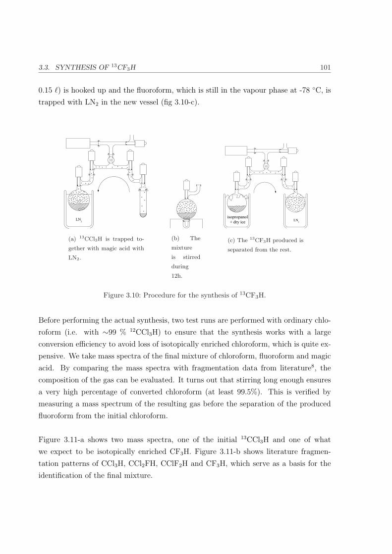
3.3. SYNTHESIS OF 13CF3H 101
0.15 `) is hooked up and the fluoroform, which is still in the vapour phase at -78 C, is
trapped with LN2 in the new vessel (fig 3.10-c).
(a) 13CCl3H is trapped to-
gether with magic acid with
LN2.
(b) The
mixture
is stirred
during
12h.
(c) The 13CF3H produced is
separated from the rest.
Figure 3.10: Procedure for the synthesis of 13CF3H.
Before performing the actual synthesis, two test runs are performed with ordinary chlo-
roform (i.e. with ∼99 % 12CCl3H) to ensure that the synthesis works with a large
conversion efficiency to avoid loss of isotopically enriched chloroform, which is quite ex-
pensive. We take mass spectra of the final mixture of chloroform, fluoroform and magic
acid. By comparing the mass spectra with fragmentation data from literature8, the
composition of the gas can be evaluated. It turns out that stirring long enough ensures
a very high percentage of converted chloroform (at least 99.5%). This is verified by
measuring a mass spectrum of the resulting gas before the separation of the produced
fluoroform from the initial chloroform.
Figure 3.11-a shows two mass spectra, one of the initial 13CCl3H and one of what
we expect to be isotopically enriched CF3H. Figure 3.11-b shows literature fragmen-
tation patterns of CCl3H, CCl2FH, CClF2H and CF3H, which serve as a basis for the
identification of the final mixture.

102 CHAPTER 3. EXPERIMENTAL SETUP
100806040200Mass [a.m.u.]
CCl3H
CF3H
(a) Mass spectra of initial gas (chloroform) and
product (essentially fluoroform).
100806040200Mass [a.m.u]
CCl3H
CCl2FH
CClF2H
CF3H
(b) Literature mass spectra8 for different hy-
drofluorochlorocarbons.
Figure 3.11: Comparison of measured and literature mass-spectra for the identification of the
gas.
The identification of the fragments is straightforward‡: the initial chloroform is readily
identified and the product is for our purposes very pure CF3H. We estimate the purity
to be & 99.5%, the transformation is quantitative.
Figure 3.12 shows a mass spectrum of the isotopically enriched 13CF3H produced. The
peaks are shifted by one mass with respect to the peaks for the test synthesis of 12CF3H.
The sample is isotopically very clean, and 12CF3H created from residual 12CCl3H is not
detectable. Recording action spectra with IRLAPS confirm this as well, as no 12CF3H
is detected. An additional peak at 85 amu is probably SiF4 created by the traces of
H2O forming H2F2 which in turn reacts on the glass surface to form SiF49. Its absence
in the mass spectrum for the synthesised 12CF3H is not very clear but probably due to
the fact that we stirred the reactive mixture for a shorter time.
This way we estimate to have produced ∼0.2 ` of isotopically enriched 13CF3H at 1 bar.
‡The relative intensities of the peaks are not the same. This is likely because of different characteristics
(detection efficiencies, ioniser, ...) of our QMS and the ones used to obtain the published mass-spectra8.

3.3. SYNTHESIS OF 13CF3H 103
100806040200
Mass [amu]
13CF3H
SiF4
Figure 3.12: Mass spectrum of the final products of the 13CF3H synthesis.

104 CHAPTER 3. EXPERIMENTAL SETUP
Bibliography
[1] M. Polianski, O. V. Boyarkin, and T.R. Rizzo. Collisionally-assisted, highly-selective
laser isotope separation of carbon-13 . J. Chem. Phys., 121(23):11771–11779, 2004.
[2] L. Rubio, M. Santos, and J. A. Torresano. Laser induced fluorescence detection of
CF, CF2 and CF3 in the infrared multiphoton dissociation of C3F6 . J. Photochem.
Photobiol. A: Chem., 146:1–8, 2001.
[3] David S. King, Peter K. Schenck, and John C. Stephenson. Spectroscopy and
Photophysics of the CF2A1B1 - X1A1 System . J. Molec. Spectrosc., 78:1–15, 1979.
[4] Mikhail N. Polianski. Overtone pre-excitation - Infrared Multiple Photon Disso-
ciation Under Collisional Conditions. New Potential for Laser Isotope Separation .
PhD thesis, Ecole polytechnique federale de Lausanne, Switzerland, 2004.
[5] Julien Pitteloud. Construction d’un Ramanshifter . Projet d’ingenieur. EPFL,
2002. The report can be obtained upon request from the author of this thesis.
[6] Lester Andrews, Helge Willner, and Frank T. Prochaska. A Simple Synthesis
for Carbon-13 Enriched Fluorochloromethanes and Fluoromethanes . J. Fluorine
Chem., 13:273–278, 1979.
[7] Robert C. Weast and Melvin J. Astle, editors. CRC Handbook of Chemistry and
Physics. CRC Press Inc., Florida, 59th edition, 1978.
[8] E. Stenhagen, S. Abrahamsson, and F. W. McLafferty. Atlas of Mass Spectral Data.
Volume I. New York: Interscience, 1969.
[9] Amanz Ruf (LCPM EPFL Switzerland). Private communication .
Chapter 4
Experimental investigations
This chapter deals with our experimental investigations. In the recently developed
method of molecular laser isotope separation (MLIS) by selectively dissociating pre-
excited CF3H molecules, we have observed an increase of isotopic selectivity upon an
increase of the sample pressure and/or the time-delay between the two lasers involved
(see section 1.2). We propose two possible mechanisms for this observation: isotopically
selective collisional relaxation of vibrationally excited molecules and different absorp-
tion rates of IR photons for the two different isotopomers. Our goal is to determine the
relative contributions of these mechanisms. Here we present the experimental methods
and ideas employed for this study.
4.1 Introduction
4.1.1 General idea
In figure 4.1 we show the general energy level diagram used in our MLIS process and
the main parameters that can be varied for the investigation of the mechanisms leading
to an increase of isotopic selectivity due to collisions.
105
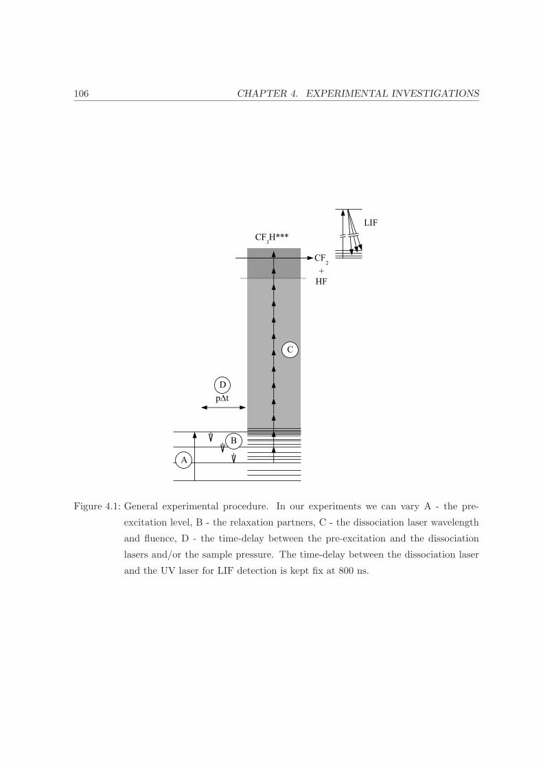
106 CHAPTER 4. EXPERIMENTAL INVESTIGATIONS
Figure 4.1: General experimental procedure. In our experiments we can vary A - the pre-
excitation level, B - the relaxation partners, C - the dissociation laser wavelength
and fluence, D - the time-delay between the pre-excitation and the dissociation
lasers and/or the sample pressure. The time-delay between the dissociation laser
and the UV laser for LIF detection is kept fix at 800 ns.

4.1. INTRODUCTION 107
We wish to keep the IRMPD step free from collisions and hence fix a low pressure of
typically 1 mbar (see section 3.2). We show in table 4.1 four schemes that can be used
for the investigation, based on varying or fixing the parameters A-D shown in figure 4.1.
Scheme A B C D Comment
]1 × This way, we investigate only the IRMPD step,
eliminating collisional effects.
Measure the dissociation yield as a function of
the time-delay between the lasers, for different...
]2 × × ... pre-excitation energies
]3 × × ... collision partners
]4 × × ... dissociation laser fluence and wavelength
Table 4.1: Four schemes for the investigation of the mechanisms of the enhancement of isotopic
selectivity varying different parameters (× A-D).
Based upon these different schemes, we propose the following experiments:
• Experiments described in section 4.2 follow scheme ]2: here we scan the time-delay
between the pre-excitation and the dissociation lasers for different pre-excitation
energies. This way, we get information about the influence of the initial rovibra-
tional state of the molecule on the relaxation and IRMPD processes. This helps
to determine the state specificity of the increase of isotopic selectivity upon an
increase of the time-delay between the two lasers.
• Experiments described in section 4.3 follow scheme ]1: here we measure the dis-
sociation probability of vibrationally excited 12CF3H and 13CF3H molecules as a
function of the CO2 dissociation laser fluence and wavelength. By measuring such
photofragment excitation spectra of CF3H molecules excited via the 31 band we
are able to get information about the dissociation process.
• Experiments described in section 4.4 follow scheme ]4: by adequately changing the
dissociation laser wavelength we can compare the disappearance of the molecules
upon a time-delay between the pre-excitation and the dissociation laser under
conditions, where IRMPD is the same for the two isotopomers. This way, we
eliminate any effects of isotopically selective IRMPD.
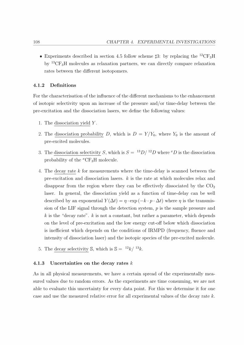
108 CHAPTER 4. EXPERIMENTAL INVESTIGATIONS
• Experiments described in section 4.5 follow scheme ]3: by replacing the 12CF3H
by 13CF3H molecules as relaxation partners, we can directly compare relaxation
rates between the different isotopomers.
4.1.2 Definitions
For the characterisation of the influence of the different mechanisms to the enhancement
of isotopic selectivity upon an increase of the pressure and/or time-delay between the
pre-excitation and the dissociation lasers, we define the following values:
1. The dissociation yield Y .
2. The dissociation probability D, which is D = Y/Y0, where Y0 is the amount of
pre-excited molecules.
3. The dissociation selectivity S, which is S = 13D/ 12D where xD is the dissociation
probability of the xCF3H molecule.
4. The decay rate k for measurements where the time-delay is scanned between the
pre-excitation and dissociation lasers. k is the rate at which molecules relax and
disappear from the region where they can be effectively dissociated by the CO2
laser. In general, the dissociation yield as a function of time-delay can be well
described by an exponential Y (∆t) = η · exp (−k · p ·∆t) where η is the transmis-
sion of the LIF signal through the detection system, p is the sample pressure and
k is the “decay rate”. k is not a constant, but rather a parameter, which depends
on the level of pre-excitation and the low energy cut-off below which dissociation
is inefficient which depends on the conditions of IRMPD (frequency, fluence and
intensity of dissociation laser) and the isotopic species of the pre-excited molecule.
5. The decay selectivity S, which is S = 12k/ 13k.
4.1.3 Uncertainties on the decay rates k
As in all physical measurements, we have a certain spread of the experimentally mea-
sured values due to random errors. As the experiments are time consuming, we are not
able to evaluate this uncertainty for every data point. For this we determine it for one
case and use the measured relative error for all experimental values of the decay rate k.
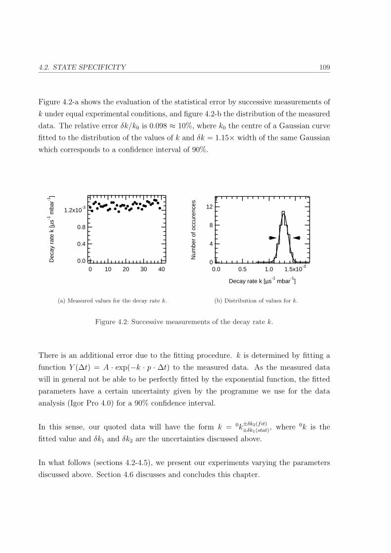
4.2. STATE SPECIFICITY 109
Figure 4.2-a shows the evaluation of the statistical error by successive measurements of
k under equal experimental conditions, and figure 4.2-b the distribution of the measured
data. The relative error δk/k0 is 0.098 ≈ 10%, where k0 the centre of a Gaussian curve
fitted to the distribution of the values of k and δk = 1.15× width of the same Gaussian
which corresponds to a confidence interval of 90%.
1.2x10⁻³
0.8
0.4
0.0Dec
ay r
ate
k [µ
s-1 m
bar-1
]
403020100
(a) Measured values for the decay rate k.
12
8
4
0
Num
ber
of o
ccur
ence
s
1.5x10⁻³
1.00.50.0
Decay rate k [µs-1
mbar-1
]
(b) Distribution of values for k.
Figure 4.2: Successive measurements of the decay rate k.
There is an additional error due to the fitting procedure. k is determined by fitting a
function Y (∆t) = A · exp(−k · p · ∆t) to the measured data. As the measured data
will in general not be able to be perfectly fitted by the exponential function, the fitted
parameters have a certain uncertainty given by the programme we use for the data
analysis (Igor Pro 4.0) for a 90% confidence interval.
In this sense, our quoted data will have the form k = 0k±δk2(fit)±δk1(stat), where 0k is the
fitted value and δk1 and δk2 are the uncertainties discussed above.
In what follows (sections 4.2-4.5), we present our experiments varying the parameters
discussed above. Section 4.6 discusses and concludes this chapter.

110 CHAPTER 4. EXPERIMENTAL INVESTIGATIONS
4.2 State specificity of the increase of isotopic selectivity upon
leaving a time-delay between the pre-excitation and the
dissociation lasers
4.2.1 Introduction
Our molecular laser isotope separation (MLIS) scheme consists of pre-exciting 13CF3H
molecules via the 31 band with a subsequent selective dissociation of pre-excited molecules
by a CO2 laser (called “dissociation laser”). The pre-excitation laser excites a small frac-
tion of 12CF3H too which results in the dissociation products not being isotopically pure.
Experimentally it has been observed that by increasing the time-delay between the two
lasers and/or by increasing the sample pressure, the isotopic selectivity increases. In
other words, the rates 12k and 13k at which the molecules lose enough vibrational energy
due to collisions such that they are not effectively dissociation by the CO2 laser any
more, are different. The question arises as to whether these different rates are due to
the fact the the rovibrational identities of the excited 12CF3H and 13CF3H are not the
same (with the chosen wavelength of the pre-excitation laser 13CF3H is excited via the
Q-branch, 12CF3H via a P-branch) or whether the energy can be considered to be ran-
domly distributed over the molecule and no state specific vibrational relaxation and/or
multiple photon dissociation (MPD) occurs.
In order to study this question, the pre-excitation laser is set to a particular rovi-
brational transition of 12CF3H or 13CF3H, the dissociation laser wavelength and fluence
is kept fixed and the rates k are determined by scanning the time-delay between the pre-
excitation and the dissociation lasers. These rates (called “decay rates”) are measured
for different pre-excitation wavelengths (resulting in different rovibrational identities of
the pre-excited molecules). The energy level diagram followed in these experiments is
shown in figure 4.3.
4.2.2 Results
We perform measurements of the decay rate k by scanning the time-delay between the
pre-excitation and the dissociation lasers for different pre-excited rovibrational states.
4.2. STATE SPECIFICITY 111
Figure 4.3: Energy scheme used in the experiments for the determination state specificity of
relaxation rates.
In a first step, we change the rotational identity of the pre-excited state, and in a second
step we change the vibrational identity too.
(I) Rotational identity
First, we compare the decay rate k for the P(32) transition of the 31 band at 12,927.78
cm−1 with k for molecules pre-excited via the Q-branch of the 31 band (for 12CF3H).
We measure decay rates of 2.92±0.13(fit)±0.29(stat) ·10−3 and 2.89
±0.07(fit)±0.29(stat) ·10−3 ns−1 mbar−1 for
pre-excitation via the P-branch and via the Q-branch. A measurable influence of the
rotational identity of the pre-excited state is not observed. We show in figure 4.4-a the
measured LIF signals as a function of the time-delay between the pre-excitation and dis-
sociation lasers for 12CF3H molecules pre-excited via the Q-branch and via a P-branch
of the 31 band. In a second step, we scan the wavelength of the pre-excitation laser

112 CHAPTER 4. EXPERIMENTAL INVESTIGATIONS
across the Q-branch of the 41 pre-excitation level for the 12CF3H molecule, and measure
decay rates k for different pre-excitation wavelengths. Within the Q-branch of the 41
pre-excitation level, we measure decay rates of 3.45±0.19(fit)±0.35(stat) ·10−3, 3.37
±0.13(fit)±0.34(stat) ·10−3,
3.60±0.14(fit)±0.36(stat) ·10−3 and 3.55
±0.14(fit)±0.36(stat) ·10−3 ns−1 mbar−1 for pre-excitation frequencies
of 11,564.75, 11,565.00, 11,565.25 and 11,565.50 cm−1. We show in figure 4.4-b the
measured decay rates as a function of the pre-excitation energy.
1000
800
600
400
200
0
LIF
sig
nal [
a.u.
]
200150100500
∆tPE-IRMPD [ns]
...via Q-branch
Pre-excitation...via P-branch
(a) Relaxation of vibrationally excited 12CF3H
molecules pre-excited via the Q-branch and a
P-branch (the curves are offset with respect to
each other for clarity).
4x10⁻³
3
2
1
0
k [n
s-1 m
bar-1
]
1156611565115641156311562
Pre-excitation [cm-1
]
(b) Action spectrum around the 41 peak of12CF3H such as the decay rates measured at
the respective wavelengths. The four different
measurements are separated by 0.25 cm−1.
Figure 4.4: Experiments to test the influence of the rotational identity of the pre-excited state
on the decay rates.
We conclude that the rotational identity of the pre-excited state does not influence the
decay rates.
(II) Vibrational identity
In a second step, we compare different pre-excited vibrational states. We measure
decay rates of molecules of both isotopic species pre-excited via the 31 and via the 32
bands. For 12CF3H, we measure decay rates of 4.70±0.05(fit)±0.47(stat) ·10−3 and 4.50
±0.04(fit)±0.45(stat)
·10−3 ns−1 mbar−1 and for 13CF3H, we measure decay rates of 1.75±0.02(fit)±0.18(stat) ·10−3 and
1.71±0.025(fit)±0.17(stat) ·10−3 ns−1 mbar−1. The decay rates are independent on the pre-excitation
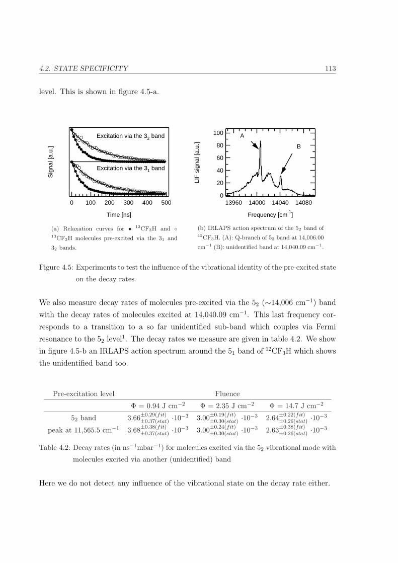
4.2. STATE SPECIFICITY 113
level. This is shown in figure 4.5-a.
Sig
nal [
a.u.
]
5004003002001000
Time [ns]
Excitation via the 32 band
Excitation via the 31 band
(a) Relaxation curves for • 12CF3H and 13CF3H molecules pre-excited via the 31 and
32 bands.
100
80
60
40
20
0LI
F s
igna
l [a.
u.]
14080140401400013960
Frequency [cm-1
]
A
B
(b) IRLAPS action spectrum of the 52 band of12CF3H. (A): Q-branch of 52 band at 14,006.00
cm−1 (B): unidentified band at 14,040.09 cm−1.
Figure 4.5: Experiments to test the influence of the vibrational identity of the pre-excited state
on the decay rates.
We also measure decay rates of molecules pre-excited via the 52 (∼14,006 cm−1) band
with the decay rates of molecules excited at 14,040.09 cm−1. This last frequency cor-
responds to a transition to a so far unidentified sub-band which couples via Fermi
resonance to the 52 level1. The decay rates we measure are given in table 4.2. We show
in figure 4.5-b an IRLAPS action spectrum around the 51 band of 12CF3H which shows
the unidentified band too.
Pre-excitation level Fluence
Φ = 0.94 J cm−2 Φ = 2.35 J cm−2 Φ = 14.7 J cm−2
52 band 3.66±0.29(fit)±0.37(stat) ·10−3 3.00±0.19(fit)
±0.30(stat) ·10−3 2.64±0.22(fit)±0.26(stat) ·10−3
peak at 11,565.5 cm−1 3.68±0.38(fit)±0.37(stat) ·10−3 3.00±0.24(fit)
±0.30(stat) ·10−3 2.63±0.38(fit)±0.26(stat) ·10−3
Table 4.2: Decay rates (in ns−1mbar−1) for molecules excited via the 52 vibrational mode with
molecules excited via another (unidentified) band
Here we do not detect any influence of the vibrational state on the decay rate either.

114 CHAPTER 4. EXPERIMENTAL INVESTIGATIONS
4.2.3 Discussion
From these experiments we conclude that the exact rovibrational identity of the pre-
excited molecules does not influence the decay rates. We can hence treat the vibrational
energy as randomly distributed over all vibrational modes of the molecule although the
experiments do not include fast collisionally induced IVR prior to vibrational energy
transfer and IRMPD. This means that we can study the behaviour of the 12CF3H
molecule by pre-exciting it via the Q-branch of a transition as its behaviour is the same
as when we excite it via a P-branch.
4.3 Properties of collision-free IRMPD of excited molecules:
photofragment excitation spectrum and dissociation selec-
tivity of vibrationally excited CF3H
In this section we present some experiments in which we study the IRMPD step of our
MLIS scheme in the absence of vibrational relaxation, which is avoided by using low
working pressures and a zero time-delay between the two laser.
4.3.1 Introduction
First, we present measurements of photofragment spectra of CF3H molecules pre-excited
to the 31 level. For this, the pre-excitation laser is tuned to the Q-branch of 12CF3H
or 13CF3H, the timing between the pre-excitation, dissociation and LIF lasers is kept
fixed, and the wavelength of the CO2 dissociation laser is changed. The dissociation
yield as a function of the dissociation laser wavelength (at a given fluence) results in a
photofragment excitation spectrum. This set of experiments aims at verifying to what
extent the MPD step is selective. The energy level diagram followed in these experi-
ments is shown in figure 4.6. In order to get good signal, we use a pulsed alexandrite
laser (PAL) instead of a Nd:YAG pumped dye laser for the pre-excitation step.
In a second step we present some complementary information, where we directly com-
pare the dissociation probabilities of 12CF3H and 13CF3H as a function of the CO2 laser
fluence and wavelength using a Nd:YAG pumped dye laser for the pre-excitation of the
molecules. In principle this information can be deduced from the data obtained using

4.3. PROPERTIES OF COLLISION-FREE IRMPD OF EXCITED MOLECULES 115
Figure 4.6: Energy scheme used in the experiments for the determination of photofragment
excitation spectra of excited molecules.
the PAL, but as we are able to measure the dissociation yields for pre-excited 12CF3H
and pre-excited 13CF3H in a same experiment, it is clear that a direct comparison of
the dissociation probabilities of 13CF3H and 12CF3H is more precise than comparing
data that has been acquired independently. The energy level diagram followed in these
experiments is the same as for the measurement of photofragment excitation spectra
shown in figure 4.6.
We present in sections 4.3.2 and 4.3.3 the results for these two experiments, in sec-
tion 4.3.4 we discuss the results and we finally make some conclusive remarks in sec-
tion 4.3.5.

116 CHAPTER 4. EXPERIMENTAL INVESTIGATIONS
4.3.2 Results: photofragment excitation spectra
The goal is to measure the dissociation yield at a fixed fluence of the dissociation laser as
a function of the dissociation laser wavelength. However, we cannot choose or attenuate
this fluence continuously, because both the maximum fluence (figure C.5 on page 251)
and the attenuation of the laser beam by the teflon sheets (figure C.1 on page 248) varies
from line to line. For this reason we measure at a given dissociation wavelength the
dissociation yield at different fluences such that we can adequately interpolate the data
for any fluence in the measured range. From this data we can construct a dissociation
yield spectrum.
Figure 4.7 shows two examples of measured dissociation yield as a function of fluence for
two different fixed values of ν. In order to do an interpolation of the dissociation yield for
any fluence Φ a fitting function is used (Y (Φ) = exp (C1 · exp (−D1 · Φ) + C2 · exp (−D2 · Φ))).
300
250
200
150
100
50
0
Dis
soci
atio
n yi
eld
[a.u
.]
543210
Dissociation laser fluence [J cm-2
]
(a) Dissociation yield of 12CF3H pre-excited
via the 31 band for a dissociation frequency
1051.3 cm−1.
250
200
150
100
50
0
Dis
soci
atio
n yi
eld
[a.u
.]
121086420
Dissociation laser fluence [J cm-2
]
(b) Dissociation yield of 13CF3H pre-excited
via the 31 band for a dissociation frequency
1083.5 cm−1.
Figure 4.7: Sample curves of measured dissociation yields.
Figure 4.8 shows two sample cuts of Y (Φ, ν) in the other dimension, i.e. keeping the
dissociation laser fluence Φ fixed and varying ν. Assuming that in the limit of high
fluence the dissociation step is saturated (i.e. the dissociation probability is unity), we
can convert the dissociation yields Y into dissociation probabilities D by normalising
the signals with the value of Y at saturation. This way, we construct the photofragment

4.3. PROPERTIES OF COLLISION-FREE IRMPD OF EXCITED MOLECULES 117
spectrum D(ν) which is the dissociation probability as a function of the dissociation
laser frequency.
1.0
0.8
0.6
0.4
0.2
0.0
Dis
soci
atio
n pr
obab
ility
1150110010501000950
Dissociation laser frequency [cm-1
]
(a) Dissociation yield of 12CF3H pre-excited via
the 31 band for a fluence of the CO2 laser of
Φ = 2 J cm−2.
1.0
0.8
0.6
0.4
0.2
0.0Dis
soci
atio
n pr
obab
ility
1150110010501000950
Dissociation laser frequency [cm-1
]
(b) Dissociation yield of 13CF3H pre-excited via
the 31 band for a fluence of the CO2 laser of
Φ = 4 J cm−2.
Figure 4.8: Sample curves of measured dissociation probability.
For convenience, we describe the dissociation yield curves with the following function‡:
Dsat(ν) = 1− exp
(−B · exp
(−
(ν − ν0
ω
)2))
(4.1)
B, ν0 and ω are fitting constants and depend on the fluence Φ of the CO2 laser: ν0
is the centre of the band, ω the width and B is a measure of saturation. For B ¿ 1,
which corresponds to the unsaturated case, we have
Dsat(ν) ≈ B · exp
(−
(ν − ν0
ω
)2)
, (4.2)
which is a gaussian curve centred at ν0 and with a width ω. Curves obeying equation 4.1
‡The overall dissociation step is the result of multiple absorption steps. We assume that the absorption
spectrum σi(ν) for every single absorption step i to have a Gaussian dependence on laser wavelength, so the
photofragment spectrum D(ν) =∏i
σi(ν) is also Gaussian. In order to take into account saturation effects,
the amount of dissociated molecules is given by2 Dsat(ν) = 1 − exp (−c · Φ ·D(ν)) where Φ is the fluence
of the dissociation laser and c is an adequate scaling parameter. This relation can be easily identified with
equation 4.1.

118 CHAPTER 4. EXPERIMENTAL INVESTIGATIONS
are fitted to the experimental data for different fluences of the CO2 laser. Unfortunately
we only have parts of the photofragment spectra due to the limited tuning range of the
CO2 laser, which makes the uncertainties on the fitted constants relatively large (see
figure 4.8). Figure 4.9 shows the values of ν0, ω and B obtained for the 12CF3H and
the 13CF3H isotopomers for different fluences.
1080
1070
1060
1050
1040
ν 0 [c
m-1
]
6543210
Dissociation laser fluence [J cm-2
]
(25 ± 10) cm-1
(a) ν0
60
50
40
30
20
10
0
ω [c
m-1
]
6543210
Dissociation laser fluence [J cm-2
]
(b) ω
10
8
6
4
2
0
B
6543210
Dissociation laser fluence [J cm-2
]
(c) B
Figure 4.9: ν0, ω and B found for the photofragment spectra of excited 12CF3H and 13CF3H
for different fluences of the CO2 laser.
• 12CF3H, 13CF3H
The following statements can be made about the dependence of fitted values ν0, ω and

4.3. PROPERTIES OF COLLISION-FREE IRMPD OF EXCITED MOLECULES 119
B on the dissociation laser fluence Φ:
• The centre ν0 does not change significantly upon increasing the Φ. The differ-
ence between the centres for 12CF3H and 13CF3H lies around ∼25 cm−1, which
corresponds to the isotopic shift of the absorption spectrum of the ν5 band in the
vibrational ground state.
• The width ω for 13CF3H seems to increase slightly upon an increase of Φ, for12CF3H the uncertainties are too large to make any statements. The origin of this
broadening may either be unreal, or, if it is real, due to power broadening: we
estimate a typical broadening‡ of ∼1 cm−1 for a fluence of 3 J cm−2.
• B, which is a measure of the saturation, is a linear function of Φ, which is also
expected considering the footnote on page 117. For 12CF3H there is a slight offset:
B is 0 for Φ ≈ 0.4 J cm−2, which demonstrates the non-linearity of MPD. This
value is coherent with a previously measured3 IRMPD threshold of 0.2-0.3 J cm−2.
For 13CF3H this “threshold” seems to be negative, but the uncertainties on the
values of B are relatively large.
The measured photofragment spectra demonstrate the red shift of the absorption spectra
as the molecules gain vibrational energy. The centre at ∼1070 cm−1 (for 12CF3H) lies
well to the red with respect to the centre of the absorption spectra of CF3H in the
vibrational ground state, which lies at 1158 cm−1. It is also shifted to lower frequencies
with respect to the photofragment spectra of CF3H molecules in the ground state, where
appreciable dissociation is measured4 only for frequencies higher than ∼1080 cm−1.
4.3.3 Results: dissociation selectivity
Here we compare the dissociation probabilities of 12CF3H and 13CF3H pre-excited via the
31 band under collision-free conditions. The dissociation probability does not depend on
the rotational state of the pre-excited molecule5. We measure the dissociation selectivity
S, which is defined as follows:
‡At higher laser radiation fields, absorption features are broadened by a Lorentzian of a width of δE. This
power broadening is δE = µ ·E where µ is the transition dipole moment of the pumped mode, ν5, and E is the
electric field from the laser radiation. The electric field can be calculated from the relation S = ε0cE2 where S
is the energy flux, c is the speed of light and ε0 is the electric constant.
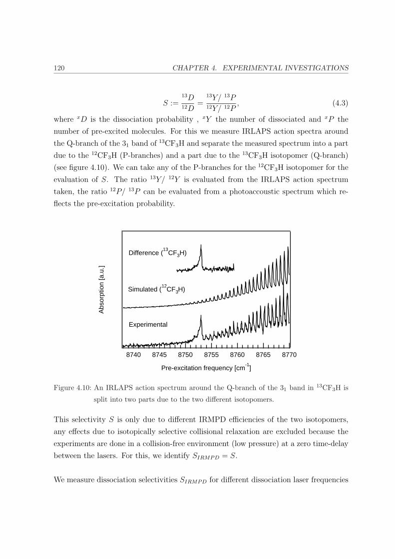
120 CHAPTER 4. EXPERIMENTAL INVESTIGATIONS
S :=13D12D
=13Y/ 13P12Y/ 12P
, (4.3)
where xD is the dissociation probability , xY the number of dissociated and xP the
number of pre-excited molecules. For this we measure IRLAPS action spectra around
the Q-branch of the 31 band of 13CF3H and separate the measured spectrum into a part
due to the 12CF3H (P-branches) and a part due to the 13CF3H isotopomer (Q-branch)
(see figure 4.10). We can take any of the P-branches for the 12CF3H isotopomer for the
evaluation of S. The ratio 13Y/ 12Y is evaluated from the IRLAPS action spectrum
taken, the ratio 12P/ 13P can be evaluated from a photoaccoustic spectrum which re-
flects the pre-excitation probability.
Abs
orpt
ion
[a.u
.]
8770876587608755875087458740
Pre-excitation frequency [cm-1
]
Simulated (12
CF3H)
Experimental
Difference (13
CF3H)
Figure 4.10: An IRLAPS action spectrum around the Q-branch of the 31 band in 13CF3H is
split into two parts due to the two different isotopomers.
This selectivity S is only due to different IRMPD efficiencies of the two isotopomers,
any effects due to isotopically selective collisional relaxation are excluded because the
experiments are done in a collision-free environment (low pressure) at a zero time-delay
between the lasers. For this, we identify SIRMPD = S.
We measure dissociation selectivities SIRMPD for different dissociation laser frequencies
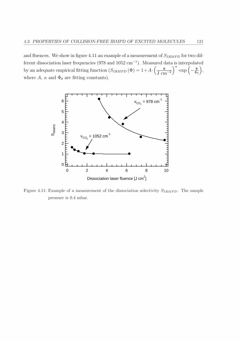
4.3. PROPERTIES OF COLLISION-FREE IRMPD OF EXCITED MOLECULES 121
and fluences. We show in figure 4.11 an example of a measurement of SIRMPD for two dif-
ferent dissociation laser frequencies (978 and 1052 cm−1). Measured data is interpolated
by an adequate empirical fitting function (SIRMPD (Φ) = 1+A·(
Φ
J cm−2
)α
·exp(− Φ
Φ0
),
where A, α and Φ0 are fitting constants).
6
5
4
3
2
1
0
SIR
MP
D
1086420
Dissociation laser fluence [J cm2]
νCO2 = 978 cm
-1
νCO2 = 1052 cm
-1
Figure 4.11: Example of a measurement of the dissociation selectivity SIRMPD. The sample
pressure is 0.4 mbar.

122 CHAPTER 4. EXPERIMENTAL INVESTIGATIONS
We show in figure 4.12 the dissociation selectivities SIRMPD for two laser fluences (2
and 9 J cm−2) for pre-excitation via the 31 band. There is a very clear dependence of
SIRMPD on the wavelength of the CO2 laser. The ratio of the dissociation probabilities
SIRMPD increases significantly to SIRMPD À 1 as we tune the dissociation laser wave-
length out of resonance. As we have shown in section 4.3 the absolute yield however
decreases considerably at the same time.
6
1
2
4
6
10
2
4
6
100
2
SIR
MP
D
10801060104010201000980960940
Dissociation laser frequency [cm-1
]
Figure 4.12: Dissociation selectivity SIRMPD for 3 J cm−2 and • 9 J cm−2.
I The — full and - - dashed lines are obtained by dividing the fitted curves
(equation 4.1) to the photofragment spectra for 12CF3H and 13CF3H presented
in section 4.3 by each other (for a fluence of 9 J cm−2 the fitting parameters in
equation 4.1 are extrapolated from the data for 1-5 J cm−2). For a fluence of 3
J cm−2 the curves do not fit the datapoints very well which shows the limits of
our fitting function.
I For the · · · dotted line, see text in section 4.3.4.
We also measure SIRMPD for molecules pre-excited through the 21 band, i.e. they are
promoted up to ∼5950 cm−1 before dissociation. For this pre-excitation energy, we
measure SIRMPD for a dissociation laser frequency of 1047 cm−1. Figure 4.13 shows the
measurements such as the equivalent data for molecules pre-excited through the 31 band.

4.3. PROPERTIES OF COLLISION-FREE IRMPD OF EXCITED MOLECULES 123
60
50
40
30
20
10
0
SIR
MP
D
3.53.02.52.01.51.00.50.0
Dissociation laser fluence [J cm-2
]
vCH = 2
vCH = 3
Figure 4.13: Dissociation selectivity SIRMPD for molecules pre-excited via the • 31 and via
the 21 bands for a dissociation laser frequency of 1047 cm−1.
For the region between 0.4 and 3 J cm−2 an enhancement of isotopic selectivity of up to
30 is measured (for Φ ≈ 0.4 J cm−2) as the pre-excitation energy is lowered from 8800
to 5950 cm−1. This increase is measured under collision-free conditions and is only due
to different IRMPD effiencies.
4.3.4 Discussion
We can tentatively try to explain the measured photofragment spectra and the disso-
ciation selectivities by a simple model as follows. The photofragment spectrum is, in
principle, a product of single absorption steps
D(ν) = σ1(ν) · σ2(ν) · . . . · σn(ν), (4.4)
where σi(ν) is the absorption probability of step i. With the knowledge of fundamental
frequencies and the spectroscopic anharmonic constants of a molecule, it is possible to
evaluate the absorption spectrum of a molecule with a vibrationally energy E. As will
be shown later (see section 5.1), we estimate this spectrum σE(ν) to be:

124 CHAPTER 4. EXPERIMENTAL INVESTIGATIONS
σE(ν) ' A(E)
ω(E)√
π· exp
(−
(ν − ν0(E)
ω(E)
)2)
, (4.5)
where
A(E) = 1 + 2.08 · 10−4 ·(
E
cm−1
)
ω(E) =
√(15.9cm−1)
2+ (3.05 · 10−3 · E)2
ν0(E) = 1158cm−1 − 6.35 · 10−3 · E .
(4.6)
The photofragment spectrum of a molecule pre-excited to 8800 cm−1 (vCH = 3) is given
by equation 4.4 where the product goes over all intermediate steps between 8800 and
24,000 cm−1 which is the dissociation limit.
If we try to calculate the photofragment spectrum using this Ansatz, we see that there
is a large discrepancy between the simulated and measured photofragment spectra: al-
though the centre of the photofragment spectrum of, for example, vibrationally excited13CF3H is correctly predicted at ∼1045 cm−1, the width is well underestimated (12
cm−1 compared to 35-45 cm−1 measured experimentally). We show in figure 4.14 data
measured for a dissociation laser fluence of 2 J cm−2 and the corresponding dissociation
yields predicted with equation 4.4.
This figure demonstrates that our model for the calculation of dissociation yields is too
simple. For the numerical reproduction of the measured data, we need to use more so-
phisticated simulations. For the explanation of the dissociation yields, a simple model
consisting of a multiplication of the subsequent absorption steps, is not enough. This
is because we do not take into account any non-linearity effects of the single absorption
steps, and stimulated emission of photons is neglected too. Furthermore, we should
adapt a dynamical picture of the subsequent absorption steps rather than simply multi-
ply absorption spectra. We present in section 5.3 master equation calculations including
all these effects.
Concerning the dissociation selectivity the following can be stated:
• For molecules pre-excited via the 31 band, substantial isotopic selectivity is gained

4.3. PROPERTIES OF COLLISION-FREE IRMPD OF EXCITED MOLECULES 125
1.0
0.8
0.6
0.4
0.2
0.0
Dis
soci
atio
n pr
obab
ility
1150110010501000950
Dissociation laser frequency [cm-1
]
Figure 4.14: Comparison of • - - experimental and — predicted dissociation yields for vibra-
tionally excited 13CF3H.
for off-resonant dissociation laser frequencies (.1000 cm−1). For typical wave-
lengths used for laser isotope separation, selectivity is only gained for moderate
and low fluences of the dissociation laser radiation.
• The behaviour of SIRMPD as a function of the frequency of the dissociation laser
frequency can be understood as follows (see figure 4.12 on page 122). The disso-
ciation yield Y of excited molecules has roughly a Gaussian dependence on the
frequency ν of the CO2 laser (see section 4.3.2). Within this approximation, the
dissociation selectivity is
SIRMPD(ν) =13Y (ν)12Y (ν)
=exp
(−( ν−ν13
ω )2)
exp(−( ν−ν12
ω )2)
∝ exp(−2·ν·(ν12−ν13)
ω2
),
(4.7)
where ν12 and ν13 are the centres of the Gaussians describing the dissociation
probabilities and ω is the width. An exponential dependence of SIRMPD on ν
is predicted (equation 4.7). The data on figure 4.12 does not suggest such an
126 CHAPTER 4. EXPERIMENTAL INVESTIGATIONS
exponential behaviour. However, at central frequencies around 1040-1060 cm−1
the dissociation yields are partly saturated and the dissociation probability is
hence not well described by a Gaussian in that region. Fitting an exponential to
the dissociation selectivity for frequencies below 1000 cm−1 where the dissociation
is far from saturation (see figure 4.8 on page 117) yields a slope of ∼0.097 (dotted
line in figure 4.12) which gives, using ν12−ν13 = 25 cm−1, a value of 23 cm−1 for ω
which compares well with the values obtained by the direct measurements of the
photofragment excitation spectra (ω ≈ 30-40 cm−1, see figure 4.9-b).
• For a dissociation laser frequency of 1047 cm−1, the dissociation yield selectivity
is greatly enhanced using vibrational pre-excitation up to vCH = 2 instead of
vCH = 3, especially for moderate and low dissociation laser fluences. In particular,
we cannot make any statements concerning the increase of isotopic selectivity of
a factor of 16 upon an adequate increase of pressure and time-delay between the
lasers previously observed for CF3H molecules pre-excited via the 31 band6, as the
experimental conditions are not exactly the same. This 16 fold increase may or
may not be explained only by different IRMPD rates.
4.3.5 Conclusions
We have measured photofragment excitation spectra and dissociation selectivities of
vibrationally pre-excited (vCH = 3) CF3H molecules. The experimental conditions (in
particular the zero time-delay between the pre-excitation and dissociation lasers and
the low pressures) are such that any effects of vibrational relaxation are excluded and
any dissociation selectivities are only due to different IRMPD rates. We have measured
a typical shift of ∼ 25 cm−1 between the photofragment excitation spectra of excited12CF3H and excited 13CF3H, which demonstrates that the shift of the ground state
absorption spectra (25 cm−1) is maintained upon excitation. We have determined the
width of the photofragment excitation spectrum of molecules pre-excited to the second
overtone of the C-H stretch vibration: first, by a direct measurement of this spectrum
(section 4.3.2) and then by comparison of the dissociation yield for excited 12CF3H and13CF3H (section 4.3.3). The values compare well: ω ≈ 20 − 30 cm−1 determined by
direct measurement and ω ≈ 23 cm−1 determined by comparison of the dissociation
yields of the two different isotopomers.

4.3. PROPERTIES OF COLLISION-FREE IRMPD OF EXCITED MOLECULES 127
Further we have determined strong dependencies of the photofragment excitation spec-
tra on the dissociation laser fluence which complicates the data analysis strongly, and
we showed that for a better understanding of our results we need to perform master
equation calculations.
4.4 Separation of different mechanisms changing the wave-
length of the dissociation laser
4.4.1 Introduction
In this section we present experiments where we investigate the influence of different
vibrational relaxation rates on the increase of isotopic selectivity upon an increase of
the time-delay between the pre-excitation and the dissociation lasers. For this, we use
the result obtained previously in section 4.3: the properties of the IRMPD step are the
same for 12CF3H and 13CF3H if the wavelength of the dissociation laser is shifted by 25
cm−1 to the red for excited 13CF3H with respect to the wavelength used to dissociate
excited 12CF3H.
In these experiments the pre-excitation laser is first set to the Q-branch of an over-
tone of the CH stretching-bending vibration of 12CF3H, the fluence of the dissociation
laser is kept fixed and its frequency is set to a certain value ν. The time-delay between
the pre-excitation and the dissociation lasers is scanned and the decay rate 12k is de-
termined from this. This value is compared to 13k measured the same way, pre-exciting13CF3H at its Q-branch and using a dissociation laser frequency of ν - 25 cm−1. The
energy level diagram followed in these experiments is shown in figure 4.15.
4.4.2 Results
Experiments are performed for molecules pre-excited via the 31 (∼8800 cm−1) and via
the 41 (∼11,500 cm−1) bands. We present the results we obtain for molecules pre-excited
to ∼8800 cm−1 in some detail, the procedures for molecules pre-excited to ∼11,500 cm−1
are in principle exactly the same. The final results are presented for both cases at the
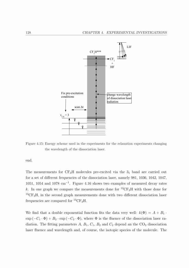
128 CHAPTER 4. EXPERIMENTAL INVESTIGATIONS
Figure 4.15: Energy scheme used in the experiments for the relaxation experiments changing
the wavelength of the dissociation laser.
end.
The measurements for CF3H molecules pre-excited via the 31 band are carried out
for a set of different frequencies of the dissociation laser, namely 981, 1036, 1042, 1047,
1051, 1054 and 1078 cm−1. Figure 4.16 shows two examples of measured decay rates
k. In one graph we compare the measurements done for 12CF3H with those done for13CF3H, in the second graph measurements done with two different dissociation laser
frequencies are compared for 13CF3H.
We find that a double exponential function fits the data very well: k(Φ) = A + B1 ·exp (−C1 · Φ) + B2 · exp (−C2 · Φ), where Φ is the fluence of the dissociation laser ra-
diation. The fitting parameters A, B1, C1, B2 and C2 depend an the CO2 dissociation
laser fluence and wavelength and, of course, the isotopic species of the molecule. The

4.4. SEPARATION OF DIFFERENT MECHANISMS CHANGING THE WAVELENGTHOF THE DISSOCIATION LASER 129
5x10⁻³
4
3
2
1
0
k [n
s-1 m
bar-1
]
151050
Dissociation laser fluence [J cm-2
]
(a) Decay rate k for the • 12CF3H and
the 13CF3H isotopomers at a frequency of
1078 cm−1 of the CO2 laser.
3.0x10⁻³
2.0
1.0
0.0
k [n
s-1 m
bar-1
]
151050
Dissociation laser fluence [J cm-2
]
(b) Decay rate k for the 13CF3H isotopomer,
for a frequency of • 1078 and ¥ 981 cm−1 of
the CO2 laser.
Figure 4.16: Sample measurements of the decay rate k. The errorbars are fitting errors (see
section 4.1.3).
function is purely empirical.
With this information, we can evaluate k at a fix fluence for different dissociation
laser frequencies used in our experiments. Figure 4.17 shows an example of interpolated
values of k obtained this way, for a fluence of 3 J cm−2.
A linear function, k(ν) = A + B · ν seems to be a reasonable fit for the data points
on figure 4.17, where A and B are fitting parameters and depend on the fluence of the
dissociation laser and the isotopic species.
4.4.3 Discussion
For the data analysis, the effect of different IRMPD rates can be eliminated if we
compare measurements using a CO2 laser frequency ν for 13CF3H and ν + 25 cm−1 for12CF3H. Thus, we define the ratio
SV ET (ν, Φ) :=k12(ν, Φ)
k13(ν − 25cm−1, Φ), (4.8)
where kx(ν, Φ) is the decay rate of xCF3H at a dissociation laser frequency ν and fluence
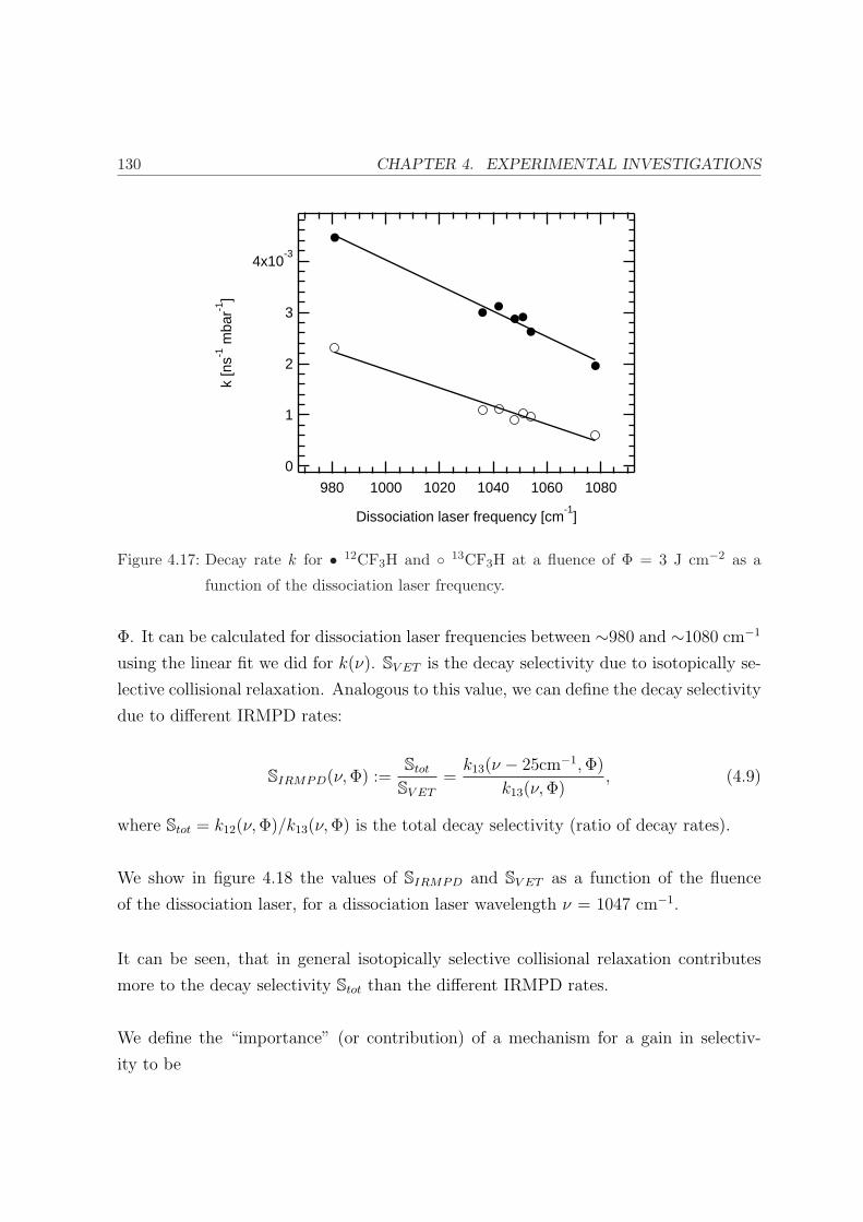
130 CHAPTER 4. EXPERIMENTAL INVESTIGATIONS
4x10⁻³
3
2
1
0
k [n
s-1 m
bar-1
]
10801060104010201000980
Dissociation laser frequency [cm-1
]
Figure 4.17: Decay rate k for • 12CF3H and 13CF3H at a fluence of Φ = 3 J cm−2 as a
function of the dissociation laser frequency.
Φ. It can be calculated for dissociation laser frequencies between ∼980 and ∼1080 cm−1
using the linear fit we did for k(ν). SV ET is the decay selectivity due to isotopically se-
lective collisional relaxation. Analogous to this value, we can define the decay selectivity
due to different IRMPD rates:
SIRMPD(ν, Φ) :=Stot
SV ET
=k13(ν − 25cm−1, Φ)
k13(ν, Φ), (4.9)
where Stot = k12(ν, Φ)/k13(ν, Φ) is the total decay selectivity (ratio of decay rates).
We show in figure 4.18 the values of SIRMPD and SV ET as a function of the fluence
of the dissociation laser, for a dissociation laser wavelength ν = 1047 cm−1.
It can be seen, that in general isotopically selective collisional relaxation contributes
more to the decay selectivity Stot than the different IRMPD rates.
We define the “importance” (or contribution) of a mechanism for a gain in selectiv-
ity to be

4.4. SEPARATION OF DIFFERENT MECHANISMS CHANGING THE WAVELENGTHOF THE DISSOCIATION LASER 131
2.0
1.5
1.0
0.5
0.0
SIR
MP
D
1086420
Dissociation laser fluence [J cm-2
]
(a) SIRMPD
3.0
2.5
2.0
1.5
1.0
0.5
0.0
SV
ET
1086420
Dissociation laser fluence [J cm-2
]
(b) SV ET
Figure 4.18: SIRMPD and SV ET determined by changing the wavelength of the CO2 dissocia-
tion laser for pre-excitation via the — 31 and the - - 41 bands.
Ix :=Sx − 1∑
i
(Si − 1), (4.10)
where x = IRMPD and VET (this way IIRMPD + IV ET = 1).
Following equation 4.10 for the evaluation of the relative importance of a mechanism
to the increase of isotopic selectivity, we evaluate the relative contributions shown in
table 4.3 to the enhancement of the isotopic selectivity upon leaving a time-delay be-
tween the pre-excitation and dissociation lasers.
IV ET IIRMPD
31 0.67 0.33
41 0.70 0.30
Table 4.3: Relative contributions of isotopically selective collisional relaxation and isotopically
selective IRMPD to the enhancement of isotopic selectivity, for a dissociation laser
fluence of 3 J cm−2 and frequency of 1047 cm−1.
We show in figure 4.19 the importance of the isotopically selective collisional relaxation
and isotopically selective IRMPD rates for a dissociation laser wavelength 1047 cm−1
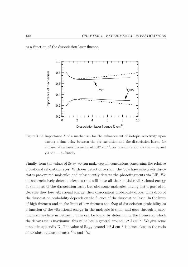
132 CHAPTER 4. EXPERIMENTAL INVESTIGATIONS
as a function of the dissociation laser fluence.
1.0
0.8
0.6
0.4
0.2
0.0
Impo
rtan
ce o
f mec
hani
sm
1086420
Dissociation laser fluence [J cm-2
]
IVET IIRMPD
Figure 4.19: Importance I of a mechanism for the enhancement of isotopic selectivity upon
leaving a time-delay between the pre-excitation and the dissociation lasers, for
a dissociation laser frequency of 1047 cm−1, for pre-excitation via the — 31 and
via the - - 41 bands.
Finally, from the values of SV ET we can make certain conclusions concerning the relative
vibrational relaxation rates. With our detection system, the CO2 laser selectively disso-
ciates pre-excited molecules and subsequently detects the photofragments via LIF. We
do not exclusively detect molecules that still have all their initial rovibrational energy
at the onset of the dissociation laser, but also some molecules having lost a part of it.
Because they lose vibrational energy, their dissociation probability drops. This drop of
the dissociation probability depends on the fluence of the dissociation laser. In the limit
of high fluences and in the limit of low fluences the drop of dissociation probability as
a function of the vibrational energy in the molecule is small and goes through a max-
imum somewhere in between. This can be found by determining the fluence at which
the decay rate is maximum: this value lies in general around 1-2 J cm−2. We give some
details in appendix D. The value of SV ET around 1-2 J cm−2 is hence close to the ratio
of absolute relaxation rates 12κ and 13κ:

4.5. SEPARATION OF DIFFERENT MECHANISMS USING A CARBON-13 ENRICHEDSAMPLE 133
SV ET ≈13κ12κ
(4.11)
With this, we determine the ratio of relaxation rates of 1.91 for molecules pre-excited
through the 31 band and 1.65 for molecules pre-excited through the 41 band, that is12CF3H relaxes 1.91 (1.65) times faster on itself than 13CF3H on 12CF3H.
Note that the ratio of relaxation rates 12κ/13κ depends on the internal energy. The
selectivity in collisional relaxation decreases upon an increase of the level of vibrational
pre-excitation (here, from 8800 up to 11,500 cm−1).
4.4.4 Conclusion
By measuring decay rates k as a function of the frequency of the dissociation laser,
we can eliminate the influence of a difference in IRMPD efficiencies of the two iso-
topomers on the observed isotopic selectivity. First, this allows us to quantify the
relative contributions of isotopically selective collisional relaxation and isotopically se-
lective IRMPD to the increase of isotopic selectivity upon leaving a time-delay between
the pre-excitation and dissociation lasers. At the same time, we have determined the
relative relaxation rates of excited 12CF3H and excited 13CF3H on 12CF3H molecules in
the ground state: we have determined that for molecules pre-excited via the 31 band12CF3H relaxes ∼1.91 times faster than 13CF3H, and for molecules pre-excited via the
41 band they relax ∼1.65 times faster.
4.5 Separation of different mechanisms using a carbon-13 en-
riched sample
4.5.1 Introduction
In this section we present experiments where we investigate the influence of different
IRMPD rates and different vibrational relaxation rates on the increase of isotopic se-
lectivity upon an increase of the time-delay between the pre-excitation and dissociation
lasers. By using 13CF3H as relaxation partner for excited xCF3H molecules instead of12CF3H (which is the main relaxation partner in a normal isotopic abundant gas) we are
able to directly separate the mechanisms of isotopically selective VET and isotopically

134 CHAPTER 4. EXPERIMENTAL INVESTIGATIONS
selective IRMPD to the different decay rates. The production of 13CF3H is described
in section 3.3.
In these experiments the pre-excitation laser is set to the Q-branch of an overtone
of the CH stretching-bending vibration of 13CF3H, the dissociation laser fluence and
wavelength are kept fixed and the time-delay between the two lasers is scanned. This
way we measure the decay rates k(x?−y) where x, y = 12, 13 which is the rate at which
the xCF3H molecules disappear from the dissociation window when relaxing on yCF3H
in the ground state. For practical reasons, we measure this decay rates for different mix-
tures of 12CF3H and 13CF3H (always keeping the total pressure at 1 mbar), fit a linear
dependence to k as a function of the isotopic composition of the sample and extrapolate
to 0 and 100% of 13CF3H. The energy level diagram followed in these experiments is
shown in figure 4.20.
4.5.2 Results
We present experiments where the decay rate k is measured for different pre-excitation
energies (pre-excitation via 21, 31, 41 and 52 bands) and dissociation laser fluences as a
function of the isotopic mixture of the sample.
As for experiments presented previously we measure the decay rates as a function of
the CO2 laser fluence because k depends on this fluence. By measuring such data for
different isotopic mixtures of the sample gas (keeping the total pressure always at 1
mbar), we measure the decay rate k as a function of the fraction f of 13CF3H in the
sample. Figure 4.21 shows an example of such a measurement.
Several points are observed:
1. The decay rate k depends on the isotopic composition of the sample.
2. The decay rates are larger when the collision partners are 13CF3H molecules.
The first statement is not trivial and it indicates that collisional vibrational relaxation
of CF3H is isotopically selective.
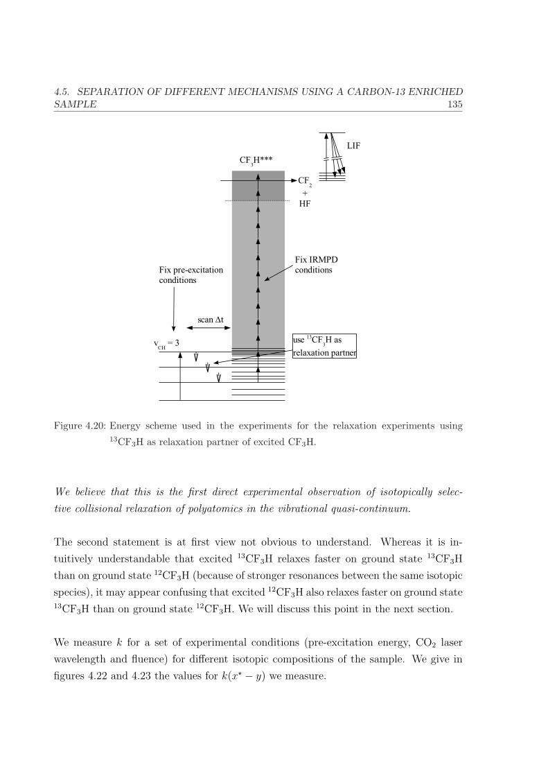
4.5. SEPARATION OF DIFFERENT MECHANISMS USING A CARBON-13 ENRICHEDSAMPLE 135
Figure 4.20: Energy scheme used in the experiments for the relaxation experiments using13CF3H as relaxation partner of excited CF3H.
We believe that this is the first direct experimental observation of isotopically selec-
tive collisional relaxation of polyatomics in the vibrational quasi-continuum.
The second statement is at first view not obvious to understand. Whereas it is in-
tuitively understandable that excited 13CF3H relaxes faster on ground state 13CF3H
than on ground state 12CF3H (because of stronger resonances between the same isotopic
species), it may appear confusing that excited 12CF3H also relaxes faster on ground state13CF3H than on ground state 12CF3H. We will discuss this point in the next section.
We measure k for a set of experimental conditions (pre-excitation energy, CO2 laser
wavelength and fluence) for different isotopic compositions of the sample. We give in
figures 4.22 and 4.23 the values for k(x? − y) we measure.

136 CHAPTER 4. EXPERIMENTAL INVESTIGATIONS
12x10-3
10
8
6
4
2
0
k [n
s-1 m
bar-1
]
1.00.80.60.40.20.0
Fraction f of 13
CF3H in sample
12* on 12
12* on 13
13* on 12
13* on 13
Figure 4.21: Example of measurement of the decay rate k for different isotopic composition
of the sample for • 12CF3H and 13CF3H. This example is obtained for CF3H
molecules pre-excited via the 41 band, for a dissociation laser fluence of 0.4 J cm−2
and a dissociation laser frequency of 1047 cm−1. The errorbars are fitting errors
(see section 4.1.3).
In the next two sections we propose an interpretation of the data presented in figures 4.22
and 4.23. We start with a qualitative interpretation (section 4.5.3) and later analyse
the data on a quantitative level (section 4.5.4).
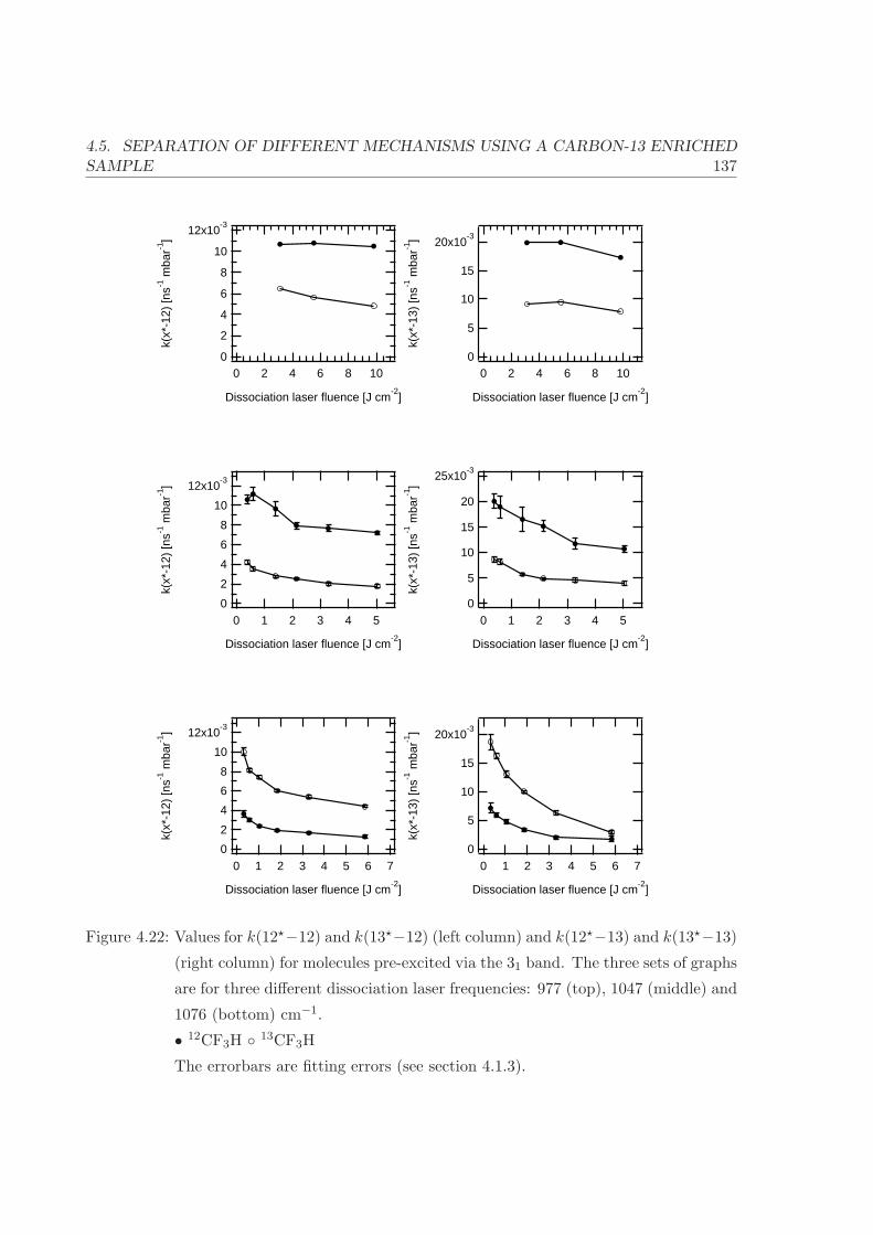
4.5. SEPARATION OF DIFFERENT MECHANISMS USING A CARBON-13 ENRICHEDSAMPLE 137
20x10-3
15
10
5
0
k(x*
-13)
[ns-1
mba
r-1]
76543210
Dissociation laser fluence [J cm-2
]
12x10-3
10
8
6
4
2
0
k(x*
-12)
[ns-1
mba
r-1]
76543210
Dissociation laser fluence [J cm-2
]
20x10-3
15
10
5
0
k(x*
-13)
[ns-1
mba
r-1]
1086420
Dissociation laser fluence [J cm-2
]
12x10-3
10
8
6
4
2
0
k(x*
-12)
[ns-1
mba
r-1]
1086420
Dissociation laser fluence [J cm-2
]
25x10-3
20
15
10
5
0
k(x*
-13)
[ns-1
mba
r-1]
543210
Dissociation laser fluence [J cm-2
]
12x10-3
10
8
6
4
2
0
k(x*
-12)
[ns-1
mba
r-1]
543210
Dissociation laser fluence [J cm-2
]
Figure 4.22: Values for k(12?−12) and k(13?−12) (left column) and k(12?−13) and k(13?−13)
(right column) for molecules pre-excited via the 31 band. The three sets of graphs
are for three different dissociation laser frequencies: 977 (top), 1047 (middle) and
1076 (bottom) cm−1.
• 12CF3H 13CF3H
The errorbars are fitting errors (see section 4.1.3).
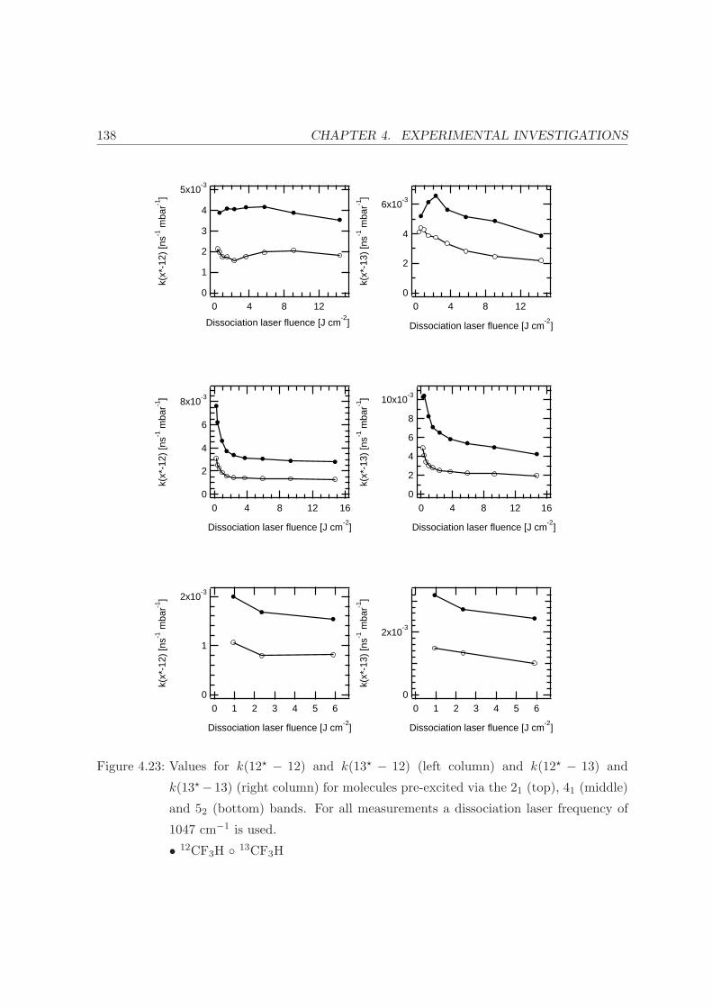
138 CHAPTER 4. EXPERIMENTAL INVESTIGATIONS
6x10⁻³
4
2
0
k(x*
-13)
[ns-1
mba
r-1]
12840
Dissociation laser fluence [J cm-2
]
5x10⁻³
4
3
2
1
0
k(x*
-12)
[ns-1
mba
r-1]
12840
Dissociation laser fluence [J cm-2
]
2x10⁻³
0
k(x*
-13)
[ns-1
mba
r-1]
6543210
Dissociation laser fluence [J cm-2
]
2x10⁻³
1
0
k(x*
-12)
[ns-1
mba
r-1]
6543210
Dissociation laser fluence [J cm-2
]
10x10-3
8
6
4
2
0
k(x*
-13)
[ns-1
mba
r-1]
1612840
Dissociation laser fluence [J cm-2
]
8x10⁻³
6
4
2
0
k(x*
-12)
[ns-1
mba
r-1]
1612840
Dissociation laser fluence [J cm-2
]
Figure 4.23: Values for k(12? − 12) and k(13? − 12) (left column) and k(12? − 13) and
k(13?− 13) (right column) for molecules pre-excited via the 21 (top), 41 (middle)
and 52 (bottom) bands. For all measurements a dissociation laser frequency of
1047 cm−1 is used.
• 12CF3H 13CF3H
4.5. SEPARATION OF DIFFERENT MECHANISMS USING A CARBON-13 ENRICHEDSAMPLE 139
4.5.3 Qualitative discussion
It is important to note that excited 12CF3H relaxes faster on the other isotopic species,13CF3H, than on itself. We explain this as follows. Vibrational energy transfer (VET)
is largely mediated by dipole-dipole interactions between the two molecules. As the
efficiency of VET depends strongly on the transition dipole moment between the ground
state and the fundamental of the corresponding vibration, the main mediator of VET
is the ν5 mode, as it has the strongest transition dipole moment. The efficiency of
this process has a reciprocal dependence on the energy mismatch between a vibrational
quantum of the donor and the acceptor molecules. This energy mismatch is, in our case,
determined by two values (see figure 4.24).
1. Anharmonic shift. Upon vibrational excitation the band origins shift to the red.
2. Isotopic shift. There is a shift of ∼25 cm−1 between the ν5 frequencies of 12CF3H
and 13CF3H (see section 4.3).
Thus, for excited 13CF3H molecules relaxing on ground state 13CF3H molecules the en-
ergy mismatch is only due to anharmonicity, while if they relax on 12CF3H there is an
additional 25 cm−1 shift which makes relaxation on 12CF3H slower than on 13CF3H. In
the case of excited 12CF3H molecules relaxing on ground state 12CF3H molecules, there
is also an energy mismatch due to the anharmonic shift. For excited 12CF3H molecules
relaxing on ground state 13CF3H molecule the isotopic and the anharmonic shifts, how-
ever, have opposite signs and cancel themselves partially, which makes relaxation of
excited 12CF3H on cold 13CF3H faster than on cold 12CF3H molecules. This idea is
illustrated in figure 4.24.
In the following section we will explain how we interpretate the experimental data
quantitatively.
4.5.4 Quantitative discussion
In this section we describe how to interpretate our results quantitatively. We describe
how to link the measured value k (the “decay rate”) with the physically relevant value
κ (the “relaxation rate”) for vibrationally excited molecules and what information we
can gain from this.
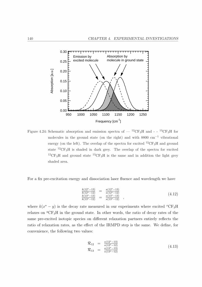
140 CHAPTER 4. EXPERIMENTAL INVESTIGATIONS
0.30
0.25
0.20
0.15
0.10
0.05
0.00
Abs
orpt
ion
[a.u
.]
125012001150110010501000950
Frequency [cm-1
]
Absorption bymolecule in ground state
Emission byexcited molecule
Figure 4.24: Schematic absorption and emission spectra of — 12CF3H and - - 13CF3H for
molecules in the ground state (on the right) and with 8800 cm−1 vibrational
energy (on the left). The overlap of the spectra for excited 12CF3H and ground
state 12CF3H is shaded in dark grey. The overlap of the spectra for excited12CF3H and ground state 13CF3H is the same and in addition the light grey
shaded area.
For a fix pre-excitation energy and dissociation laser fluence and wavelength we have
k(12?−13)k(12?−12)
= κ(12?−13)κ(12?−12)
k(13?−13)k(13?−12)
= κ(13?−13)κ(13?−12)
,(4.12)
where k(x? − y) is the decay rate measured in our experiments where excited xCF3H
relaxes on yCF3H in the ground state. In other words, the ratio of decay rates of the
same pre-excited isotopic species on different relaxation partners entirely reflects the
ratio of relaxation rates, as the effect of the IRMPD step is the same. We define, for
convenience, the following two values:
R12 = κ(12?−13)κ(12?−12)
R13 = κ(13?−13)κ(13?−12)
(4.13)

4.5. SEPARATION OF DIFFERENT MECHANISMS USING A CARBON-13 ENRICHEDSAMPLE 141
Equation 4.13 links relaxation rates of one isotopomer relaxing on different collisional
partners. We make the very important assumption that the self-relaxation rates for the
two isotopomers are the same:
κ(12? − 12) = κ(13? − 13) (4.14)
Indeed, these rates are mainly determined by the anharmonic shift of vibrations in ex-
cited molecules, which depends very little on the isotopic composition of the molecule.
Finally, we also define:
RE :=k(12? − 12)
k(13? − 13)(4.15)
With the definitions of R12, R13 and RE we can analyse our data presented in sec-
tion 4.5.2. We analyse and interpretate the results from two points of view:
1. From a fundamental point of view, what are the relative relaxation rates of the
different isotopomers relaxing on each other ?
2. What can we deduce concerning the laser isotope separation process ? When leav-
ing a time-delay ∆t between the pre-excitation and dissociation lasers, how much
selectivity is gained by isotopically selective collisional relaxation and how much is
gained due to the different IRMPD efficiencies of the two different isotopomers ?
(I) Fundamental considerations
Concerning fundamental considerations on vibrational relaxation, we plot R12 and R13
defined in equation 4.13 for different experimental conditions. This is shown in fig-
ure 4.25.
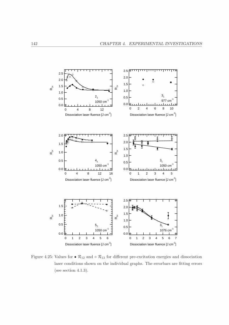
142 CHAPTER 4. EXPERIMENTAL INVESTIGATIONS
2.5
2.0
1.5
1.0
0.5
0.0
R1x
76543210
Dissociation laser fluence [J cm-2
]
31
1076 cm-1
2.5
2.0
1.5
1.0
0.5
0.0
R1x
1086420
Dissociation laser fluence [J cm-2
]
31
977 cm-1
2.5
2.0
1.5
1.0
0.5
0.0
R1x
543210
Dissociation laser fluence [J cm-2
]
31
1050 cm-1
2.5
2.0
1.5
1.0
0.5
0.0
R1x
12840
Dissociation laser fluence [J cm-2
]
21
1050 cm-1
1.5
1.0
0.5
0.0
R1x
6543210
Dissociation laser fluence [J cm-2
]
52
1050 cm-1
2.0
1.5
1.0
0.5
0.0
R1x
1612840
Dissociation laser fluence [J cm-2
]
41
1050 cm-1
Figure 4.25: Values for • R12 and R13 for different pre-excitation energies and dissociation
laser conditions shown on the individual graphs. The errorbars are fitting errors
(see section 4.1.3).

4.5. SEPARATION OF DIFFERENT MECHANISMS USING A CARBON-13 ENRICHEDSAMPLE 143
First we have to notice that the values of R12 and R13 depend on the dissociation laser
fluence. As a consequence we have to take the value for R12 and R13 at a fluence where
the dissociation yield drops off as fast as possible as the molecules relax and lose energy.
As we explained earlier, this fluence lies around 1-2 J cm−2 for standard dissociation
laser wavelengths. This way we extract the values presented in table 4.4 forR12 andR13.
Pre-excitation Pre-excitation
band energy [cm−1] R12 R13
21 5950 1.6 2.45
31 8800 1.94 1.98
41 11,530 1.9 1.75
52 14,000 1.65 1.7
Table 4.4: Experimentally measured ratio of relaxation rates.Rx = κ(x? − 13)/κ(x? − 12).
For the 31 pre-excitation band we have two measurements yielding slightly different
values for R12 and R13. We take the average between the two measurements yielding
R12 = 1.94 and R13 = 1.98. The values of R12 and R13 as a function of the vibrational
energy of the CF3H molecule are plotted in figure 4.26.
It is very interesting to notice the general trends we see on figure 4.26. For excited13CF3H, the ratio of relaxation rates on 12CF3H and on 13CF3H decreases as the pre-
excitation energy is increased from 6000 up to 14,000 cm−1. For pre-excited 12CF3H
molecules, it goes through a maximum lying at ∼10,000 cm−1.
(II) Consequences for laser isotope separation
We now analyse our data from the point of view of laser isotope separation. Remem-
ber, our initial problem was to understand how much of the selectivity gained due to
collisions is due to isotopically selective collisional relaxation and how much is due to
different IRMPD efficiencies of the two different isotopomers. The influence of the two
effects can be quantified as follows:
1. First, we want to compare the relaxation rates of excited 12CF3H on itself with

144 CHAPTER 4. EXPERIMENTAL INVESTIGATIONS
2.5
2.0
1.5
1.0
0.5
0.0
Rx
12000800040000
Energy in molecule [cm-1
]
Figure 4.26: Relative relaxation rates • R12 and R13.
the relaxation rate of excited 13CF3H on 12CF3H. This is given by the value R13
which we defined earlier:
κ(13? − 13)
κ(13? − 12)=
κ(12? − 12)
κ(13? − 12)= R13 (4.16)
2. The influence of different IRMPD efficiencies can be expressed in a similar manner,
by using the value RE defined in equation 4.15. This is because self-relaxation,
i.e. excited 12CF3H on ground state 12CF3H and excited 13CF3H on ground state13CF3H, is independent of the isotopic species (see equation 4.14).
We identify
SV ET = R13 = k(13?−13)k(13?−12)
SIRMPD = RE = k(12?−12)k(13?−13)
(4.17)
The total decay selectivity is, as expected, Stot = SV ET · SIRMPD. This can be graphi-
cally illustrated in figure 4.27.
In the laser isotope separation process where we work with a sample containing 1%
of 13CF3H the selectivity increases because the decay rate for 12CF3H (point 1 in fig-

4.5. SEPARATION OF DIFFERENT MECHANISMS USING A CARBON-13 ENRICHEDSAMPLE 145
12x10-3
10
8
6
4
2
0
k [n
s-1 m
bar-1
]
1.00.80.60.40.20.0
Fraction of 13
CF3H in sample
1
2
3
4 5
6
Figure 4.27: Interpretation of our results obtained with isotopically enriched samples. The
two solid lines on this graphs show k as a function of the isotopic composition of
the sample (upper line for 12CF3H, lower line for 13CF3H, see also figure 4.21).
Refer to the text for explanations.
ure 4.27) is faster than the decay rate for 13CF3H (point 2). The differences between
decay rates in points 1 and 3 are only due to IRMPD effects and differences between
decay rates in points 3 and 2 are only due to isotopically selective collisional relaxation.
The values of SV ET (=R13) are shown in figure 4.26. In figure 4.28 we plot the values
for SIRMPD, as a function of the dissociation laser fluence.
The “importance” (or “contribution”) I of the two mechanisms has been defined in
equation 4.10 as follows
IIRMPD = SIRMPD−1(SIRMPD−1)+(SV ET−1)
IV ET = SV ET−1(SIRMPD−1)+(SV ET−1)
,(4.18)
with IIRMPD + IV ET = 1. With this, we now can evaluate the relative contributions
to the enhancement of selectivity as a function of the different pre-excitation energies.
This is shown in figure 4.29.
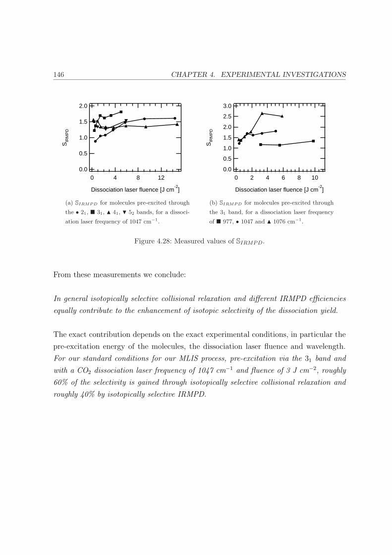
146 CHAPTER 4. EXPERIMENTAL INVESTIGATIONS
2.0
1.5
1.0
0.5
0.0
SIR
MP
D
12840
Dissociation laser fluence [J cm-2
]
(a) SIRMPD for molecules pre-excited through
the • 21, ¥ 31, N 41, H 52 bands, for a dissoci-
ation laser frequency of 1047 cm−1.
3.0
2.5
2.0
1.5
1.0
0.5
0.0
SIR
MP
D
1086420
Dissociation laser fluence [J cm-2
]
(b) SIRMPD for molecules pre-excited through
the 31 band, for a dissociation laser frequency
of ¥ 977, • 1047 and N 1076 cm−1.
Figure 4.28: Measured values of SIRMPD.
From these measurements we conclude:
In general isotopically selective collisional relaxation and different IRMPD efficiencies
equally contribute to the enhancement of isotopic selectivity of the dissociation yield.
The exact contribution depends on the exact experimental conditions, in particular the
pre-excitation energy of the molecules, the dissociation laser fluence and wavelength.
For our standard conditions for our MLIS process, pre-excitation via the 31 band and
with a CO2 dissociation laser frequency of 1047 cm−1 and fluence of 3 J cm−2, roughly
60% of the selectivity is gained through isotopically selective collisional relaxation and
roughly 40% by isotopically selective IRMPD.
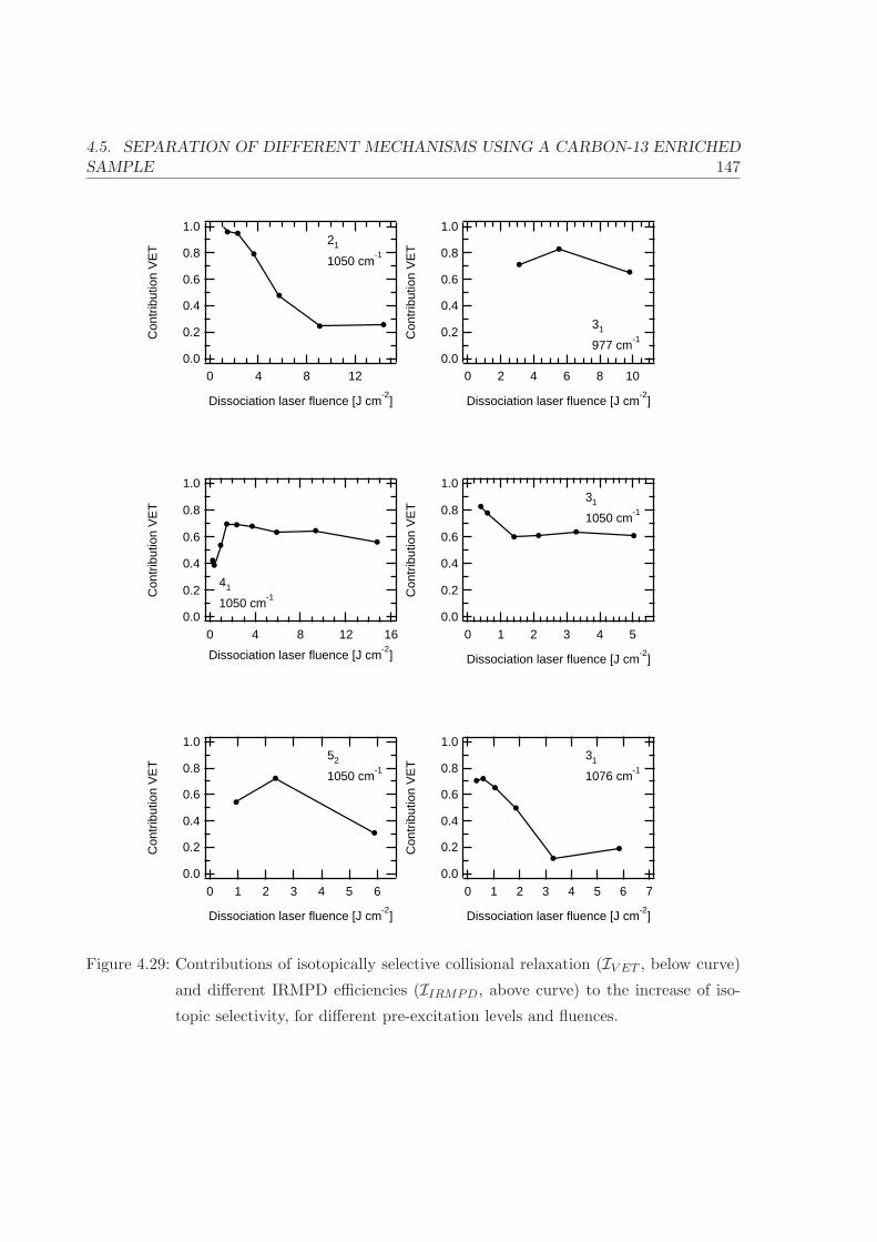
4.5. SEPARATION OF DIFFERENT MECHANISMS USING A CARBON-13 ENRICHEDSAMPLE 147
1.0
0.8
0.6
0.4
0.2
0.0
Con
trib
utio
n V
ET
1612840
Dissociation laser fluence [J cm-2
]
41
1050 cm-1
1.0
0.8
0.6
0.4
0.2
0.0
Con
trib
utio
n V
ET
6543210
Dissociation laser fluence [J cm-2
]
52
1050 cm-1
1.0
0.8
0.6
0.4
0.2
0.0
Con
trib
utio
n V
ET
76543210
Dissociation laser fluence [J cm-2
]
31
1076 cm-1
1.0
0.8
0.6
0.4
0.2
0.0
Con
trib
utio
n V
ET
1086420
Dissociation laser fluence [J cm-2
]
31
977 cm-1
1.0
0.8
0.6
0.4
0.2
0.0
Con
trib
utio
n V
ET
543210
Dissociation laser fluence [J cm-2
]
31
1050 cm-1
1.0
0.8
0.6
0.4
0.2
0.0
Con
trib
utio
n V
ET
12840
Dissociation laser fluence [J cm-2
]
21
1050 cm-1
Figure 4.29: Contributions of isotopically selective collisional relaxation (IV ET , below curve)
and different IRMPD efficiencies (IIRMPD, above curve) to the increase of iso-
topic selectivity, for different pre-excitation levels and fluences.

148 CHAPTER 4. EXPERIMENTAL INVESTIGATIONS
4.6 Discussion and conclusion
The goal of this work is to explain the increase of isotopic selectivity of our MLIS
procedure upon an increase of the sample pressure or of the time-delay between the
pre-excitation and dissociation lasers. We proposed two mechanisms: (a) isotopically se-
lective collisional relaxation and (b) different IRMPD efficiencies of the two isotopomers,
and the experiments proposed here targeted a disentanglement of the two mechanisms
for time delayed laser pulses. An additional question was whether the observed prop-
erties are general properties which can, in principle, also be found in other molecules
with similar qualitative properties as CF3H, or whether the observed increase in iso-
topic selectivity is very specific to the pre-excitation through the 31 band of CF3H. In
other words: can we treat the energy distribution in the molecule as statistical or is it
localised in a specific vibrational mode ? In a set of experiments we have addressed
these questions.
1. In section 4.2 we showed that the decay rates are not state specific. This finding
is supported by the fact that the same observation has been done for the CF2HCl
molecule7.
2. In a second step we determined the intrinsic isotopic selectivity due to the IRMPD
step only (section 4.3), at low pressures and with a zero time-delay between the
pre-excitation and dissociation lasers. We showed (see figures 4.11 and 4.12 on
pages 121 and 122) that under such conditions this selectivity is 1 for fluences of
& 2 J cm−2 if the dissociation laser is not too off-resonant (i.e. & 1000 cm−1). We
also showed that a simple model describing IRMPD as a set of multiple absorption
steps is not adequate for the description of our results, and that more sophisticated
modeling needs to be done.
3. In two different experiments (sections 4.4 and 4.5) we have studied the influence
of vibrational relaxation and the different IRMPD efficiencies on the enhancement
of isotopic selectivity due to collisions. By changing different parameters in our
experimental setup (the wavelength of the dissociation laser in the experiments
presented in section 4.4 and the relaxation partner in the experiments presented
in section 4.5), we determined the relative contributions of isotopically selective
collisional relaxation and isotopically selective IRMPD. Some of these results can
4.6. DISCUSSION AND CONCLUSION 149
be directly compared: our experiments yield the results shown in table 4.5 for
the relative importance of different IRMPD efficiencies IIRMPD and isotopically
selective collisional relaxation IV ET for a dissociation laser frequency of 1047 cm−1
and fluence of 3 J cm−2.
v = 3 v = 4
Experiment IIRMPD IV ET IIRMPD IV ET
• Change of dissociation laser frequency ∼30 % ∼70 % ∼33 % ∼67 %
• Isotopically enriched sample ∼37 % ∼63 % ∼31 % ∼69 %
Table 4.5: Results obtained for the separation of IRMPD and vibrational relaxation for a
dissociation laser frequency of 1047 cm−1 and fluence of 3 J cm−2.
Furthermore, we have determined the ratio of the relaxation rate of excited 13CF3H
and the relaxation rate of excited 12CF3H on ground state 12CF3H. The findings
are shown in figure 4.30.
Although small differences exist between the results of the two experiments are
similar, which makes us believe that the experiments, where we changed the disso-
ciation laser frequency and where we worked with isotopically enriched fluoroform,
are reliable. Thus, we may conclude:
(a) Collisional relaxation is isotopically selective. The selectivity depends on
the level of excitation (figure 4.26). For molecules with a vibrational energy
between 6000 and 14,000 cm−1, relaxation on 13CF3H is 1.5-2.5 faster than
on 12CF3H.
(b) The mechanism of the increase of isotopic selectivity upon leaving a time-delay
between the overtone and dissociation lasers consists of a joint contribution
of isotopically selective collisional relaxation and different IRMPD efficiencies
of the two isotopomers. The exact contributions depend on the fluence of the
dissociation laser and on the pre-excitation energy (figure 4.29). As one tunes
the dissociation laser frequency to the red, vibrational relaxation becomes
more and more important with respect to the IRMPD efficiencies. For typical
frequencies used for the laser isotope separation process (∼1047 cm−1), both
effects contribute roughly equally to the enhancement of isotopic selectivity.

150 CHAPTER 4. EXPERIMENTAL INVESTIGATIONS
3.0
2.5
2.0
1.5
1.0
13κ
/ 12κ
12000800040000
Energy in molecule [cm-1
]
Figure 4.30: Experimentally determined ratio of relaxation rates, measures
by changing the wavelength of the dissociation laser.
• by letting the molecules relax on 13CF3H instead of 12CF3H.
Furthermore, at these conditions and pre-excitation levels of up to vCH = 2
and vCH = 3, vibrational relaxation becomes more and more important as
the fluence of the dissociation laser is lowered.
Summarising, we were able to:
F Directly observe isotopic selective relaxation of highly excited polyatomic molecules.
F Determine their relative relaxation rates as a function of the pre-excitation energy
summarised in figure 4.26 on page 144.
F Quantify the relative contributions of the mechanisms of isotopically selective col-
lisional relaxation and of different IRMPD rates to the enhancement of isotopic
selectivity upon leaving a time-delay between the pre-excitation and the dissocia-
tion lasers.
BIBLIOGRAPHY 151
Bibliography
[1] O. V. Boyarkin, R. D. F. Settle, and T. R. Rizzo. Vibrational Overtone Spectra
of Jet-Cooled CF3H by Infrared Laser Assisted Photofragment Spectroscopy . Ber.
Bunsenges. Phys. Chem., 99(3):504–513, 1995.
[2] Richard Barry Bernstein. Chemical dynamics via molecular beam and laser tech-
niques. Oxford: Clarendon Press; New York: Oxford University Press, 1982.
[3] M. Polianski, O. V. Boyarkin, and T.R. Rizzo. Collisionally-assisted, highly-selective
laser isotope separation of carbon-13 . J. Chem. Phys., 121(23):11771–11779, 2004.
[4] J. A. O’Neill, L. Pateopol, and B. Pogue. Multiphoton absorption measurements
in CF3H . J. Phys. B: At. Mol. Opt. Phys., 25:3335–3344, 1992.
[5] R. D. F. Settle and T. R. Rizzo. CO2 laser assisted vibrational overtone spectroscopy
. J. Chem. Phys., 97(4):2823–2825, 1992.
[6] O. V. Boyarkin, M. Kowalczyk, and T. R. Rizzo. Collisionally Enhanced Isotopic
Selectivity in Multiphoton Dissociation of vibrationally excited CF3H . J. Chem.
Phys., 118(1):93–103, 2003.
[7] Thierry Krombach. Spectroscopy of CF2HCl and study of the collisional deac-
tivation taking place in laser induced isotopic separation . Master’s thesis, Ecole
polytechnique federale de Lausanne, Switzerland, 2000. The report can be obtained
upon request from the author of this thesis.

152 CHAPTER 4. EXPERIMENTAL INVESTIGATIONS

Chapter 5
Numerical simulations of V-V
energy transfer and IRMPD of
CF3H
In this section we present numerical simulations of two different parts involved in our
experiments.
1. First we have directly observed isotopically selective collisional relaxation and we
could determine the relative relaxation rates of the different isotopic species as
a function of the vibrational energy of a molecule (see section 4.5). Here, we
present a model involving vibrational relaxation both due to long-range dipole-
dipole interactions and due to short-range head-on collisions, and we show that
we can reproduce our experimental results very well.
2. Secondly, we present simulations of the laser isotope separation process involv-
ing IRMPD of vibrationally pre-excited molecules (OP-IRMPD). In this part, we
first present simulations, in which we reproduce some of our experimental findings
described in chapter 4 thus demonstrating the validity of our calculations. From
this, we then present calculations that aim to determine the relative influences of
isotopically selective collisional relaxation and selective IRMPD to the enhance-
ment of isotopic selectivity at high pressures. We also present some predictions
of the dissociation yield of vibrationally excited CF3H molecules for different ex-
perimental conditions, such as the pre-excitation energy, the sample pressure and
153
154 CHAPTER 5. NUMERICAL SIMULATIONS
the dissociation laser fluence and wavelength and some practical predictions for a
possible industrial application of the laser isotope separation process.
For both of these parts, we need to be able to calculate the absorption and the emis-
sion spectra of highly excited molecules. For this reason, this topic is singled out and
presented as an independent section.
This chapter of numerical simulations is hence built up as follows: in section 5.1 we
present the calculation of absorption and emission spectra of excited molecules, in sec-
tion 5.2 we present simulations concerning collisional vibrational relaxation and finally
in section 5.3 we present our calculations of the MLIS process.
5.1 Absorption and emission spectra of an excited molecule
Both for simulations of IRMPD and V-V energy transfer, we need to know the IR
absorption and emission spectra of an excited CF3H molecule. In this section we explain
how this is done.
5.1.1 Statistical “inhomogeneous” broadening
In this section the absorption and emission spectra‡ of excited molecules will be de-
scribed neglecting rotational effects (i.e. with ∆J = ∆K = 0). Rotational contributions
will be added in section 5.1.3. The absorption feature of excited molecules differs in two
points from ground state molecules: it shifts and it broadens.
Above a certain level of vibrational energy, this energy is no longer localised in a par-
ticular vibrational mode of the molecule, but distributed over all vibrational modes due
to IVR. The state of a molecule can be represented by
|Ψ〉 'N∑
i=1
ci| vi1, v
i2, . . . , v
in〉, (5.1)
‡The concepts for the absorption and emission spectra are very similar. Here we mainly present the results
for absorption spectra, but they can be directly transposed to emission spectra.

5.1 COMPUTATION OF ABSORPTION/EMISSION SPECTRA 155
where the sum goes over all zeroth order states | vi1, v
i2, . . . , v
in〉 which have energies close
to each other. For simplicity we will assume in our calculations that the values of |ci|2are the same (= 1/N). It has to be clearly stated that an explicit assumption is inten-
sive mixing of the vibrational states, which is not the case for vibrationally low excited
molecules.
Statistically the molecule can be in any of these zeroth order states. For the absorption
of a photon, the oscillator strength can originate from any of these zeroth order states
and is only given by the concerned matrix element.
Recall formula 2.2 giving the energy of a state with vibrational quantum numbers
v = (v1, v2, . . . , vN , lk, lk+1, . . . , lN):
E(v) =∑s
ωs
(vs + 1
2
)+
∑t
ωt (vt + 1)
+∑s≥s′
xss′(vs + 1
2
) (vs′ +
12
)
+∑t≥t′
xtt′ (vt + 1) (vt′ + 1)
+∑s,t
xst
(vs + 1
2
)(vt + 1)
+∑t≥t′
gtt′ltlt′ ,
(5.2)
where vs, vt are the vibrational quantum numbers, li are the vibrational angular momen-
tum quantum number for doubly degenerate modes, ωs, ωt are the harmonic frequencies,
and xij and gij are the spectroscopic anharmonic constants. Sums over s are for non-
degenerate modes, sums over t relate to doubly degenerate modes. This expression
neglects higher order terms which are, at least at lower vibrational energies, negligible.
At higher energies these higher order terms may grow more important, but the effect
will be at least partially washed out by the broadening described here.
When the number of quanta in a mode νp is increased by one the energy changes
by
∆E = E(v1, v2, . . . , vp + 1, . . . , vN , lk, lk+1, . . . , li ± 1, . . . , lN)
− E(v1, v2, . . . , vp, . . . , vN , lk, lk+1, . . . , li, . . . , lN)(5.3)

156 CHAPTER 5. NUMERICAL SIMULATIONS
with the selection rule ∆l = ±1 (in the case of a doubly degenerate mode). The set
of all possible ∆E constitutes the possible vibrational bands. As the number of cou-
pled states increases as the vibrational energy in the molecule goes up, the number of
possible band origins ∆E increases as well. This explains why the spectrum broadens
as the molecule gains energy1–5. In addition to the broadening, there is a shift of the
absorption spectrum; in general this shift is towards lower energies (i.e.xij < 0) which
gives the shift the name of a “red-shift”.
The broadening is often called “statistical inhomogeneous broadening” (SIB)‡. For the
calculation of vibrational spectra one has to determine all states | v1, v2, . . . , vN〉 ly-
ing within an energy region E ± ∆E and determine the band origin of the transition
| v1, v2, . . . , vp, . . . vN〉 → | v1, v2, . . . , vp ± 1, . . . , vN〉 where νp is the mode accepting or
emitting a photon in the harmonic approximation with a linear dipole function. The
matrix elements scale as6
〈vp |q| vp + 1〉 =√
vp + 1 · 〈0 |q| 1〉〈vp |q| vp − 1〉 =
√vp · 〈1 |q| 0〉
(5.4)
and hence, in the case of a non-degenerate vibration,
σ(vp → vp − 1) = vp · σ(1 → 0)
σ(vp → vp + 1) = (vp + 1) · σ(0 → 1)
σ(0 → 1) = σ(1 → 0) ,
(5.5)
where σ is the absorption (emission) cross-section. Similarly, for a doubly degenerate
vibration the strength scales as7
σ(vp, k → vp − 1) =vp + k
vp + 1· σ(1 → 0), (5.6)
where k is the vibrational angular momentum. Note that a summation over k gives a
total absorption strength for the vp → vp− 1 transition which is∑k
σ(vp, k → vp− 1) =
vp · σ(1 → 0), which is coherent with equation 5.5.
‡In general the term “inhomogeneous” refers to a system, where the broadening is caused by an ensemble
of different molecules absorbing at different wavelengths. This is not the case for this kind of broadening. We
will, in what follows, nevertheless adopt the term “inhomogeneous” broadening because it is widely accepted
in parts of the scientific community.

5.1 COMPUTATION OF ABSORPTION/EMISSION SPECTRA 157
We call the set of band origins ∆ν0 disregarding rotational contributions as a “SIB
spectrum” (SIB = statistical inhomogeneous broadening). With these considerations
and the spectroscopic anharmonic constants of a particular molecule, such SIB spectra
of excited molecules can be calculated. This is done in the next section for CF3H.
5.1.2 Vibrational absorption and emission spectra of vibrationally excited
CF3H
In this section we present calculated SIB spectra of vibrationally excited CF3H molecules.
Anharmonic constants listed previously8 (table 2.3 on page 24) are used to calculate the
shift and broadening of the absorption and emission spectra using the considerations
presented in the previous section. We calculate these spectra for excited CF3H molecules
assuming that levels over a width of 400 cm−1 mix (this is quite large, the results are
however not very sensitive to this width). The calculations of the SIB absorption and
emission spectra are done for CF3H molecules over a wide range of internal energies.
The spectra for the absorption of one quantum in ν5 are shown in figure 5.1 for the
internal energies E = 0, 2500, 5000, . . ., 20,000 cm−1. Note however, that the spectra
for low excited molecules have to be taken with care, as the mixing of the states is not
large enough for complete redistribution of energy in the molecule on the time-scales of
our experiments. The curves are included for completeness.
In figure 5.2 the same graphs for ν2, ν3 and ν6 are shown. We leave out ν1 and ν4
because they mix strongly via Fermi Resonances. This mixing is not accounted for in
equation 5.2.
The SIB spectra approach roughly a Gaussian curve as the molecules gain energy and
can be described as:
σE(ν) ' Ap(E)
δνp
√π· exp
(−
(ν − (ν0 + ∆νp)
δνp
)2)
(5.7)
The width δvp and the shift ∆vp of these Gaussians, as well as the integral intensity
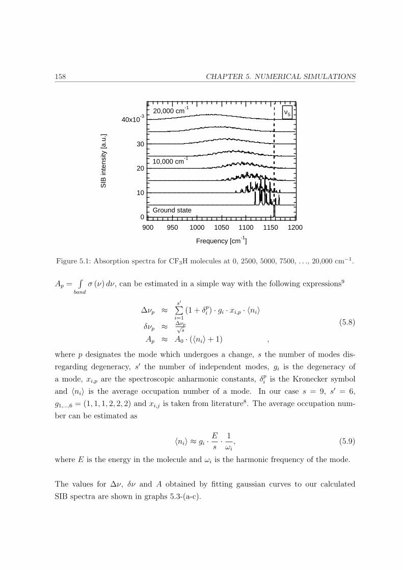
158 CHAPTER 5. NUMERICAL SIMULATIONS
40x10-3
30
20
10
0
SIB
inte
nsity
[a.u
.]
12001150110010501000950900
Frequency [cm-1
]
ν5
Ground state
10,000 cm-1
20,000 cm-1
Figure 5.1: Absorption spectra for CF3H molecules at 0, 2500, 5000, 7500, . . ., 20,000 cm−1.
Ap =∫
band
σ (ν) dν, can be estimated in a simple way with the following expressions9
∆νp ≈s′∑
i=1
(1 + δpi ) · gi · xi,p · 〈ni〉
δνp ≈ ∆νp√s
Ap ≈ A0 · (〈ni〉+ 1) ,
(5.8)
where p designates the mode which undergoes a change, s the number of modes dis-
regarding degeneracy, s′ the number of independent modes, gi is the degeneracy of
a mode, xi,p are the spectroscopic anharmonic constants, δpi is the Kronecker symbol
and 〈ni〉 is the average occupation number of a mode. In our case s = 9, s′ = 6,
g1,...,6 = (1, 1, 1, 2, 2, 2) and xi,j is taken from literature8. The average occupation num-
ber can be estimated as
〈ni〉 ≈ gi · E
s· 1
ωi
, (5.9)
where E is the energy in the molecule and ωi is the harmonic frequency of the mode.
The values for ∆ν, δν and A obtained by fitting gaussian curves to our calculated
SIB spectra are shown in graphs 5.3-(a-c).

5.1 COMPUTATION OF ABSORPTION/EMISSION SPECTRA 159
50x1
0-3 40 30 20 10 0
SIB intensity [a.u.]
520
500
480
460
440
420
400
Fre
quen
cy [c
m-1
]
ν 6
Gro
und
stat
e
10,0
00 c
m-1
20,0
00 c
m-1
40x1
0-3 30 20 10 0
SIB intensity [a.u.]
700
650
600
550
Fre
quen
cy [c
m-1
]
ν 3
Gro
und
stat
e
10,0
00 c
m-1
20,0
00 c
m-1
40x1
0-3 30 20 10 0
SIB intensity [a.u.]
1180
1160
1140
1120
1100
1080
Fre
quen
cy [c
m-1
]
ν 2
Gro
und
stat
e
10,0
00 c
m-1
20,0
00 c
m-1
Fig
ure
5.2:
SIB
abso
rpti
onsp
ectr
afo
rν 2
,ν3
and
ν 6.
The
curv
esar
efo
rvi
brat
iona
lene
rgie
sof
the
mol
ecul
esw
hich
are
mul
tipl
e
inte
gers
of25
00cm
−1.

160 CHAPTER 5. NUMERICAL SIMULATIONS
1100
1000
900
800
700
600
500
Ban
d or
igin
[cm
-1]
20000150001000050000
Energy in molecule [cm-1
]
ν5 ν2ν3
ν6
(a) Centre of SIB spectra. The slopes are given
in the first column of table 5.1.
60
40
20
0
Wid
th [c
m-1
]
20000150001000050000
Energy in molecule [cm-1
]
ν5
ν3
ν2, ν6
(b) Width of SIB spectra. The functional de-
pendence on the internal energy are of the
(empirical) form of w = A · (E/cm2) + B ·exp
(−k · (E/cm2)). The slopes for energies
larger than 5000 cm−1 are given in the second
column of table 5.1.
10
8
6
4
2
0
Rel
ativ
e to
tal a
bsor
ptio
n in
tens
ity
20000150001000050000
Energy in molecule [cm-1
]
ν6ν5, ν3
ν2
(c) Integral intensity of SIB spectra. The slopes
are given in the third column of table 5.1. The
value for the lowest frequency vibration, ν6, in-
creases the fastest, the value for the highest fre-
quency vibration, ν2, increases the slowest.
Figure 5.3: The transition spectra of excited molecules shift, broaden and get more intense as
the energy of the molecules increase.
In table 5.1 the shifts, widths and intensities are given both for the estimations using
equations 5.8 and for fitted values to the calculated SIB spectra.
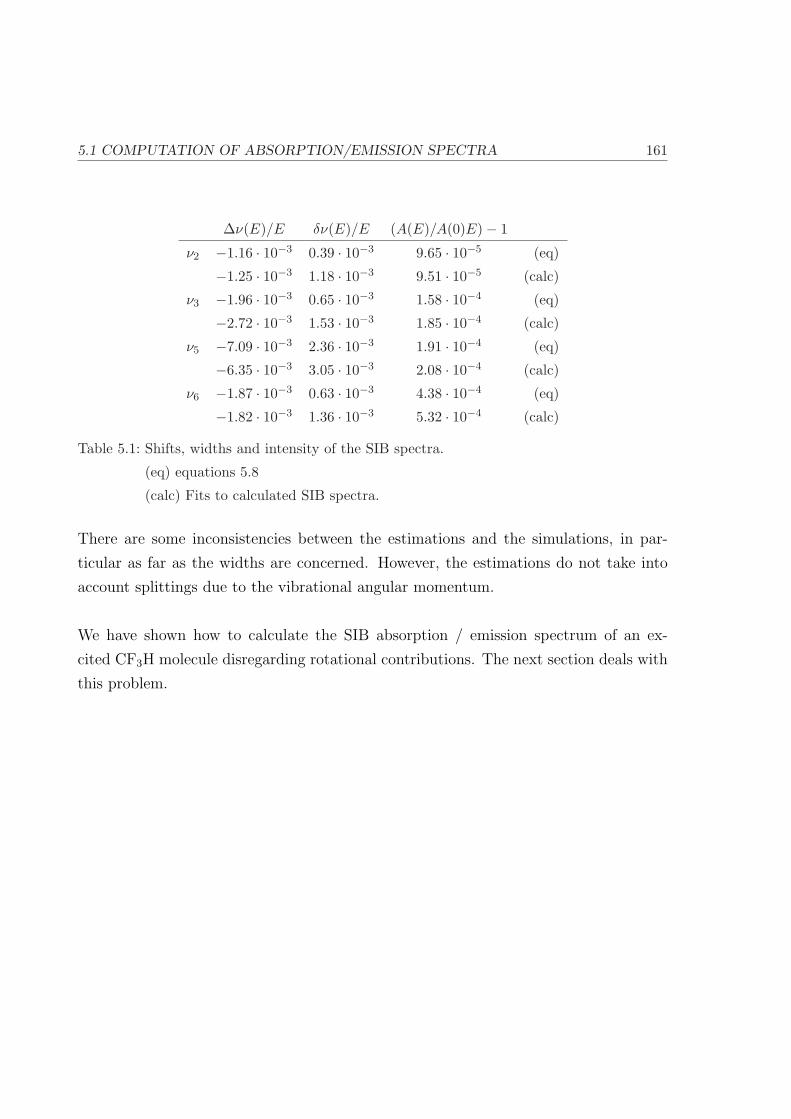
5.1 COMPUTATION OF ABSORPTION/EMISSION SPECTRA 161
∆ν(E)/E δν(E)/E (A(E)/A(0)E)− 1
ν2 −1.16 · 10−3 0.39 · 10−3 9.65 · 10−5 (eq)
−1.25 · 10−3 1.18 · 10−3 9.51 · 10−5 (calc)
ν3 −1.96 · 10−3 0.65 · 10−3 1.58 · 10−4 (eq)
−2.72 · 10−3 1.53 · 10−3 1.85 · 10−4 (calc)
ν5 −7.09 · 10−3 2.36 · 10−3 1.91 · 10−4 (eq)
−6.35 · 10−3 3.05 · 10−3 2.08 · 10−4 (calc)
ν6 −1.87 · 10−3 0.63 · 10−3 4.38 · 10−4 (eq)
−1.82 · 10−3 1.36 · 10−3 5.32 · 10−4 (calc)
Table 5.1: Shifts, widths and intensity of the SIB spectra.
(eq) equations 5.8
(calc) Fits to calculated SIB spectra.
There are some inconsistencies between the estimations and the simulations, in par-
ticular as far as the widths are concerned. However, the estimations do not take into
account splittings due to the vibrational angular momentum.
We have shown how to calculate the SIB absorption / emission spectrum of an ex-
cited CF3H molecule disregarding rotational contributions. The next section deals with
this problem.
162 CHAPTER 5. NUMERICAL SIMULATIONS
5.1.3 Rotational contribution to the absorption spectrum
For the total absorption spectra the rotational contributions have to be considered in
addition to SIB. For this, the SIB spectra are convoluted with a clean rotational contour.
The rotational energy which has already been noted in equation 2.13 are taken:
F (J,K) = B · J · (J + 1) + (C −B) ·K2, (5.10)
where B and C are rotational constants of the molecule in the ground state. Using this
rotational contour is an approximation:
• First, the values of B and C depend on the vibrational excitation. Their values
are well given by equation 2.14 on page 33. Using excitation dependent values for
B and C shifts the overall absorption spectrum by ∼ 1 cm−1 to the red.
• The rotational levels of | v5 = 1〉 interact via Coriolis interaction with rotational
levels of | v2 = 1〉 and, in a smaller extent, via Fermi interactions with rotational
levels of | v3 = 1, v6 = 1〉. The corresponding matrix elements are given as fol-
lows10–14:
〈ν5, J,K ± 1, l = ±1 |H| ν3 + ν6, J,K ± 1, l = ±1〉 = Wf
〈ν5, J,K ± 1, l = ±1 |H| ν2, J,K, l = 0〉 = ±ξ · F±(J,K)
〈ν3 + ν6, J,K − 1, l = −1 |H| ν3 + ν6, J,K + 1, l = +1〉 = −12· q6 · F+(J,K) · F−(J,K)
(5.11)
where J and K are the rotational quantum numbers, l is the vibrational quantum
number associated with the ν5 vibration,
F±(J,K) =√
J · (J + 1)−K · (K ± 1) (5.12)
and Wf = 6.5 cm−1, ξ= 0.341985 cm−1 and q6 = 11.91 ·10−4 cm−1. These inter-
actions lead to a distorted rotational contour of the 0 → n5 = 1 vibrational band.
It should be expected the higher excited states interact similarly. If one wanted
to calculate the rotational structure of a state | v1, v2, v3, v4, v5, v6〉 one would have

5.1 COMPUTATION OF ABSORPTION/EMISSION SPECTRA 163
to let it interact through Coriolis interaction with | v1, v2 + 1, v3, v4, v5 − 1, v6〉but also with | v1, v2 − 1, v3, v4, v5 + 1, v6〉 which themselves are again coupled to
| v1, v2 + 2, v3, v4, v5− 2, v6〉 and | v1, v2− 2, v3, v4, v5 + 2, v6〉 and so on. This gets a
rather difficult task, and the uncertainties on the results will become increasingly
important (nothing is known on the interaction constants Wf , ξ and q6 upon exci-
tation, and further interactions may further distort the rotational levels). In this
sense there is no real improvement if we try to include any Coriolis interactions.
The shift of the rotational contour of the 0 → n5 = 1 transition due to Coriolis in-
teractions (∼ 2-3 cm−1) is more important than the ∼ 1 cm−1 due to the vibrational
excitation dependence of the rotational constants B and C. For this reason we neglect
changes in the values of B and C upon vibrational excitation as it is smaller than the
influence of Coriolis interactions. These will also be left away because of the associated
difficulties.
The selection rules for a transition are ∆J = 0,±1 and ∆K = 0 for a ‖ transition
(ν1, ν2 and ν3) and ∆J = 0,±1 and ∆K = ±1 for a ⊥ transition (ν4, ν5 and ν6). The
intensity of the transition is given by15
I ∝ AKJ · (2J + 1) · e−F (J,K)/kBT , (5.13)
where AKJ is proportional to the square of the transition moment summed over all
orientations of J , (2J + 1) is the degeneracy of the state due to different M quantum
numbers (projection of J onto the laboratory z-axis) and the exponential is the Boltz-
mann population of the state. The values AKJ are known as the “Honl-London factors”.
The values of AKJ for a ‖ band are given by15
AKJ =
(J+1)2−K2
(J+1)·(2J+1)(∆J = +1)
K2
J ·(J+1)(∆J = 0)
J2−K2
J ·(2J+1)(∆J = −1)
(5.14)
and for a ⊥ band by

164 CHAPTER 5. NUMERICAL SIMULATIONS
AKJ =
(J+2±K)·(J+1±K)(J+1)·(2J+1)
(∆J = +1)(J+1±K)·(J∓K)
(J+1)·J (∆J = 0)(J−1∓K)·(J∓K)
J ·(2J+1)(∆J = −1) ,
(5.15)
where the upper and lower signs of ± and ∓ refer to ∆K = +1 and to ∆K = −1
respectively.
With these considerations the total absorption / emission spectrum can be easily eval-
uated by the convolution of the rotational spectrum and the SIB spectrum. This rota-
tional contour is shown in figure 5.4-a for a transition in ν5. We show in figure 5.4-b the
SIB spectrum and its convolution with the rotational structure for a CF3H molecule at
a vibrational energy of 5000 cm−1 for the absorption of one quantum in ν5.
80x10-3
60
40
20
0
Rot
atio
nal c
ontr
ibut
ion
-40 -20 0 20 40
Frequency [cm-1
]
(a) Rotational contour used for the convolution
with the SIB spectra.
6x10⁻³
4
2
0
Abs
orpt
ion
1200115011001050
Frequency [cm-1
]
(b) SIB spectrum (bottom) and its convolution
with the rotational contour (top) for a molecule
with 5000 cm−1 of vibrational energy.
Figure 5.4: For the calculation of the whole absorption spectrum the SIB spectrum is convo-
luted with a rotational contour.
Because of this convolution, the width of the gaussian approximation of the spectra
(equation 5.7) shifts. For the additional broadening consider that the convolution of
two gaussians of width δSIB and δrot is again a gaussian of width δtot =√
δ2SIB + δ2
rot.
Although both the rotational contour and the SIB spectra are not gaussians at all, it
turns out that the formula holds very well if we use a rotational width of δrot ≈ 15.9
5.2 COMPUTATION OF V-V ENERGY TRANSFER 165
cm−1.
We have shown how to take into account the rotational structure for the calculation of
the complete absorption (and emission) spectra. In summary, in the case of an absorp-
tion of one quantum in ν5, the gaussian fits to the SIB spectra have to be broadened by
a second gaussian of a width of 15.9 cm−1. Although a gaussian curve does not describe
the pure SIB spectra in an adequate manner, they are adequate for the total absorption
spectrum (including rotations) for molecules with a vibrational energy of & 3000-4000
cm−1.
5.2 Numerical simulations of vibrational energy transfer be-
tween excited and ground state molecules
In this section we present calculations concerning vibrational relaxation rates of excited
CF3H molecules on CF3H molecules in the ground state. The calculations shall be
compared with the experimental measurements presented in figure 4.26 on page 144.
First, we state the basic assumptions for these calculations, then we present our model
based on the Fermi Golden Rule (FGR). We then present the actual results and discuss
them.
5.2.1 Assumptions
For our calculations we have to make a certain number of assumptions:
1. Complete rotational relaxation. The rotational thermalisation is always com-
plete, i.e. the time between two collisions with vibrational energy transfer (VET)
is enough for the rotational relaxation to be complete(i.e. rotational relaxation
rates À vibrational relaxation rates). This condition is in general well met in
molecular systems.
2. IVR is complete. We initially pre-excite molecules through a Nj band, so the
initial vibrational state is well defined. Collision-free IVR occurs on typical time-
scales of & 100 ps (pre-excitation via 31 and 41 bands) and & 5 ps (pre-excitation
via 52 band) (see section 2.1.2.B). Furthermore, collision-induced IVR occurs with
166 CHAPTER 5. NUMERICAL SIMULATIONS
an estimated rate of 4.3 times the hard sphere collision rate‡. For these reasons
IVR can be assumed to be complete on the time-scale of our experiment.
5.2.2 V-V energy transfer mediated by dipole-dipole interactions
This section describes the calculation of rates of V-V energy transfer mediated by dipole-
dipole interactions between an excited and a ground state molecule. When two molecules
collide§ there is a certain probability that one molecule (called the donor) loses one quan-
tum in a certain mode νi and another molecule (called the acceptor) gains one quantum
in νi. In what follows, all values referring to the donor molecule will have a superscript(D), and those referring to the acceptor molecule are denoted by a (A).
The potential energy V (R, Θ, q(D)i , q
(A)i ) due to two interacting molecules depends on
the distance R between the centres of mass, the mutual orientation in space, defined by
the set of angle variables Θ and the vibrational coordinates q of the two molecules. V
can be expressed as a series in q:
V = V0(R, Θ) +∑i
V(D)i (R, Θ)q
(D)i +
∑i
V(A)i (R, Θ)q
(A)i
+∑ij
V(DD)ij (R, Θ)q
(D)i q
(D)j +
∑ij
V(AA)ij (R, Θ)q
(A)i q
(A)j +
∑ij
V(AD)ij (R, Θ)q
(A)i q
(D)j
+ . . . (higher order terms)
(5.16)
At relatively large distances it is the V(AD)ii (R, Θ)q
(A)i q
(D)i terms that are responsi-
ble for the exchange of one quantum in the mode νi. These terms represent the
dipole-dipole interaction of the two molecules. Higher order terms, represented by
V(AADD)ijkl (R, Θ)q
(A)i q
(A)j q
(D)k q
(D)l etc are for higher order pole interactions.
‡Experimentally it has been shown that for molecules pre-excited via the fundamental of the C-H stretch
vibration collision-induced IVR occurs at a rate of 1.67 · 107 s−1 torr−1 which is 1.4 times faster than the hard
sphere collision rate (see section 2.1.2.C). CI-IVR scales roughly with the vibrational energy of the molecule16,
so molecules excited via the 31 band undergo CI-IVR at a rate of ∼ 3 · 1.67 · 107 s−1 torr−1.§One has to be careful when using the term “collision” as this is not well defined. Using the term “collision”
implicitly includes that there is a relatively sharp cut-off in the distance where V-V energy transfer takes place
and where it does not. This may be applicable to a certain extent to hard collisions (see section 2.3), but
for soft collisions where the interaction potential between the colliding molecules goes as 1/rn where r is the
distance between the molecules there is no sharp cut-off. Nevertheless we use the term “collision” but we have
to bear in mind the problem associated with the expression.
5.2 COMPUTATION OF V-V ENERGY TRANSFER 167
In general, i.e. for large distances between two molecules (say R & 5 − 10 A), the
prevailing terms in equation 5.16 for V-V energy transfer are the terms representing the
dipole-dipole interactions, V(AD)ij . Because of this, we formulate the following, additional
simplification:
• In our calculations we consider only dipole-dipole interactions. To avoid the region
where higher order poles can interfere, we assume a minimum distance R0 between
two encountering molecules.
A collision between an excited molecule and a ground state molecule with internal ener-
gies E(D) and E(A) and rotational quantum numbers | J (D), K(D),M (D)〉 and | J (A), K(A),M (A)〉may result in the transfer of one quantum in the mode p of the excited molecule to the
ground state molecule. This change in vibrational quantum numbers is accompanied
by a change in rotational quantum numbers such as the energy defect caused through
the mismatch of vibrational frequencies is compensated by rotations‡.
The following selection rules apply: ∆J (D) = 0,±1, ∆J (A) = 0,±1, ∆K(D) = ±1
(for a ⊥ transition) or ∆K(D) = 0 (for a ‖ transition), and similarly ∆K(A) = ±1 or
∆K(A) = 0. In addition to this the total M , i.e. M (D) + M (A), has to be conserved.
These selection rules apply to dipole-dipole interactions and are direct consequences of
the angular dependence of V(AD)ii . For higher order interactions, which become impor-
tant at close distances, the selection rules are different (they scale with the order of the
pole).
For the calculation of the transition rate we use the Fermi Golden Rule:
W =2π
~|〈i |V | f〉|2C(E), (5.17)
where C(E) is the density of states (DOS) which depends on the vibrational energy
E of the excited molecule, | i〉 and | f〉 are the initial and final states of the pair of
molecules and V is the considered interaction. In the frame of the model outlined above
the following expression for the density of states has been derived elsewhere17–19:
‡Here we neglect translational degrees of freedom
168 CHAPTER 5. NUMERICAL SIMULATIONS
C(E) =
∫
band
Ar (ν) Er (ν) dν, (5.18)
where Ar is the absorption spectrum of the acceptor molecule and Er is the emission
spectrum of the donor molecule (see also equation 2.46 on page 60).
In principle we should perform the calculations using trajectory calculations (“dynami-
cal image”). We choose to adopt a “static image” for our calculations, which is slightly
easier to calculate. In this model, given the large number of molecules interacting pair-
wise, any mutual position between two molecules can be found somewhere in the sample,
and all mutual positions are equally probable. In this case we do not integrate over time
following the trajectory of two molecules, but we integrate over the whole space at a
given time. In principle the two models are equivalent, although there is one point that
has to be verified. If, for a given situation in the dynamical image, the transition gets
saturated (i.e. the probability of vibrational energy transfer in a collision is close to
1), the static model will overestimate the transition rate for this situation. We show in
section 5.2.3 that in our case it is justified to used the “static model” for collisions with
closest distance of ∼5-8 A.
At the first step we consider a single rotational state | J (D), K(D)〉 of the excited molecule
and calculate its relaxation rate. Then we average this rate over all possible J (D) and
K(D) quantum numbers with their respective Boltzmann weights. This allows a better
control over the calculation procedure and an easier verification of the results.
The V-V energy transfer rate of a molecule with rotational quantum numbers J and K
relaxing on a molecule in the ground state in the static picture is given by the Fermi
Golden Rule as follows16:
WJK = 2πN ·
∞∫
R0
⟨|〈i |Vd (R) | f〉|2⟩ (4πR2
)dR
·
∑
J ′K′Q (∆ωJ ′K′JK) AJ ′K′JK , (5.19)
where N is the density of molecules, 〈|〈i |Vd (R) | f〉|2〉 is |〈i |Vd (R) | f〉|2 averaged over
their mutual orientations, the integral over the distances between the two molecules,

5.2 COMPUTATION OF V-V ENERGY TRANSFER 169
AJ ′K′JK are the Honl-London factors cited previously in equations 5.14 and 5.15 and Qis the correlation of the vibrational SIB spectrum E(ν) of the excited molecule calculated
previously in section 5.1.2 and the observed ground state absorption spectrum, Ar(ν):
Q(∆ω) =
∫
band
E(ν ′)Ar(ν′ + ∆ω)dν ′ (5.20)
∆ω is the energy mismatch created by the rotational transition of the excited molecule
and reads
∆ωJKJ ′K′ = 〈B〉E · J · (J + 1)− 〈B〉E−ν5 · J ′ · (J ′ + 1)
+〈C −B〉E ·K2 − 〈C −B〉E−ν5 ·K ′2 ,(5.21)
where unprimed quantum numbers refer to the initial state and the primed numbers to
the final state of the donor molecule, and 〈B〉 and 〈C〉 are average rotational constants
at the energy E. The values of 〈B〉 and 〈C〉 can be calculated with equation 2.14.
Equations 5.17 and 5.19 are equivalent.
The interaction energy Vd between two dipole moments ~d1 and ~d2 at a certain respective
distance ~R and orientation is given by
Vd =1
4πε0
·(
(~d1~d2)
R3− 3 · (~d1
~R)(~d2~R)
R5
). (5.22)
Thus, using the initial and final states | i〉 = | i1〉| i2〉 and | f〉 = | f1〉| f2〉, we get
(4πε0) · 〈i |Vd| f〉 = (〈i1 |〈i2 |)(
(~d1~d2)
R3 − 3 · (~d1~R)(~d2
~R)R5
)(| f1〉| f2〉)
= (〈i1 |~d1| f1〉〈i2 |~d2| f2〉)R3 − 3 · (〈i1 |~d1| f1〉~R)(〈i2 |~d2| f2〉~R)
R5
= (~µ1~µ2)R3 − 3 · (~µ1
~R)(~µ2~R)
R5 ,
(5.23)
where we defined ~µ := 〈i |~d| f〉, which is called the “transition dipole moment”. The av-
erage of |〈i |Vd| f〉|2 can be calculated. We set ~µi = (µi sin φi sin θi, µi sin φi cos θi, µi cos φi)
(for i = 1, 2) and ~R = (0, 0, R). The z axis is chosen to be parallel to ~R. Then equa-
tion 5.23 becomes (with µ1 = µ2 = µ):
(4πε0)·〈i |Vd| f〉 =µ2
R3(sin φ1 sin θ1 sin φ2 sin θ2 + sin φ1 cos θ1 sin φ2 cos θ2 − 2 cos φ1 cos φ2)
(5.24)

170 CHAPTER 5. NUMERICAL SIMULATIONS
To calculate the average value 〈|〈i |Vd| f〉|2〉 the following integrations have to be per-
formed:
(4πε0)2 · ⟨|〈i |Vd| f〉|2
⟩=
π∫0
dφ1
2π∫0
dθ1
π∫0
dφ2
2π∫0
dθ2 (|〈i |Vd| f〉|2 sin φ1 sin φ2)
π∫0
dφ1
2π∫0
dθ1
π∫0
dφ2
2π∫0
dθ2 (sin φ1 sin φ2)
(5.25)
This integration has been done with the programme mathematica. The result is given
as follows:
(4πε0) ·⟨|〈i |Vd| f〉|2
⟩=
2µ4
3R6(5.26)
For convenience we define
CJK(E) =∑
J ′K′Q (∆ωJ ′K′JK) AJ ′K′JK , (5.27)
where the subscripts “JK” reflects the fact that we are treating excited molecules with
the rotational quantum numbers J and K.
Equation 5.19 may now be rewritten. It reads, after integration:
WJK =16π2µ4NCJK(E)
9R30 (4πε0)
2 (5.28)
The calculation of W , i.e. the overall relaxation rate, is done by averaging the individual
WJK over all J and K rotational states with the weights (2J+1)·exp (− (F (v, J,K) /kBT )),
where F (v, J,K) is the energy of the initial level given in equation 5.10.
We have shown how to calculate energy transfer rates using the static picture presented
here. As we have pointed out, we have to show that the energy transfer probability
for a collision is smaller than 1 in order to avoid the static model overestimating the
transfer rates. This will be done in the next section.
5.2.3 Justification of the “static model”
In this section we want to get an estimate of the conditions under which the static
model can be used. For this, we have to ensure ourselves that the vibrational energy
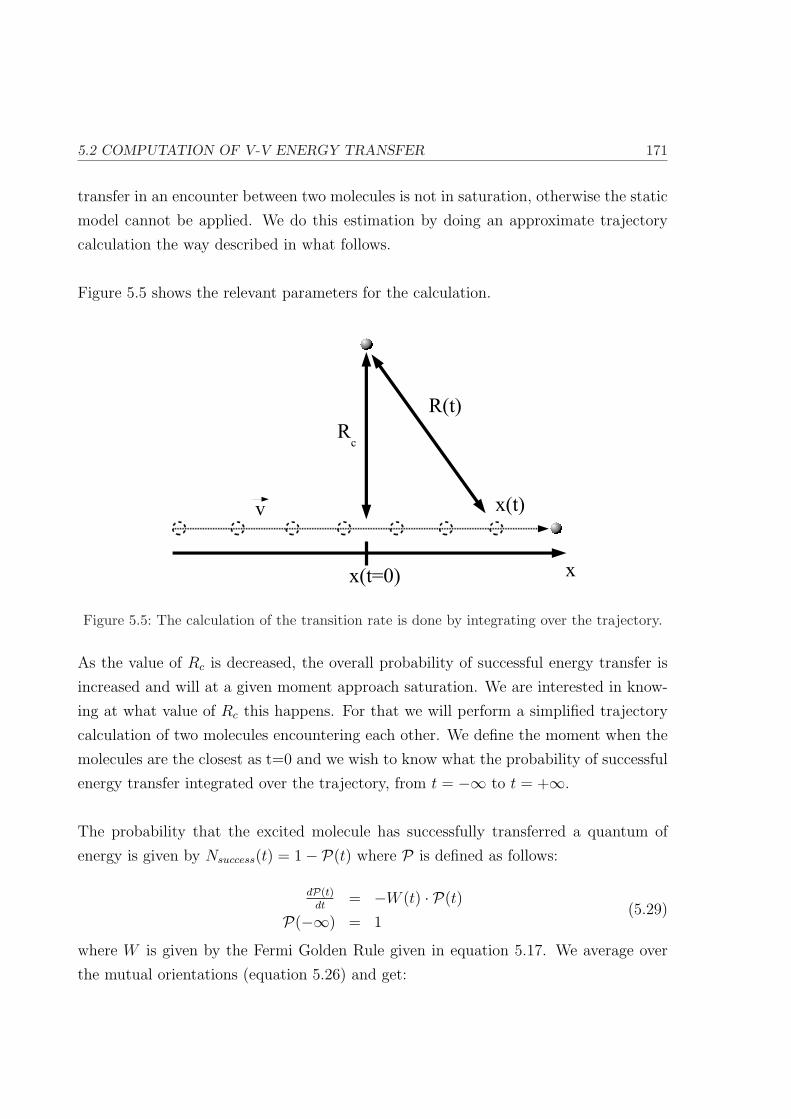
5.2 COMPUTATION OF V-V ENERGY TRANSFER 171
transfer in an encounter between two molecules is not in saturation, otherwise the static
model cannot be applied. We do this estimation by doing an approximate trajectory
calculation the way described in what follows.
Figure 5.5 shows the relevant parameters for the calculation.
Figure 5.5: The calculation of the transition rate is done by integrating over the trajectory.
As the value of Rc is decreased, the overall probability of successful energy transfer is
increased and will at a given moment approach saturation. We are interested in know-
ing at what value of Rc this happens. For that we will perform a simplified trajectory
calculation of two molecules encountering each other. We define the moment when the
molecules are the closest as t=0 and we wish to know what the probability of successful
energy transfer integrated over the trajectory, from t = −∞ to t = +∞.
The probability that the excited molecule has successfully transferred a quantum of
energy is given by Nsuccess(t) = 1− P(t) where P is defined as follows:
dP(t)dt
= −W (t) · P(t)
P(−∞) = 1(5.29)
where W is given by the Fermi Golden Rule given in equation 5.17. We average over
the mutual orientations (equation 5.26) and get:
172 CHAPTER 5. NUMERICAL SIMULATIONS
W (t) = 2π~ C 2µ4
3R(t)6(4πε0)2
= 2π~ C 2µ4
3(R2c+(v·t)2)3(4πε0)2
(5.30)
where v is the relative velocity of the two molecules. The solution of equation 5.29 is
P(t) = exp
(−A
B· 3π
16
)· exp
(−A
8·(
t (5 + 3B2t2)
(1 + B2t2)2 +3 arctan (Bt)
B
)), (5.31)
where we defined
A = 4πCµ4
3~R6c(4πε0)2
B = vRc
,(5.32)
and hence
P(t →∞) = exp
(− 4π2Cµ4
8~R5c (4πε0)
2 v
). (5.33)
or, in a more convenient form:
P(t →∞) = exp
(−2.2 · 10−2 ·
( C0.01(cm−1)−1
)·( µ
0.391D
)4
·(
10A
Rc
)5
·(
250ms−1
v
)),
(5.34)
where 0.01 (cm−1)−1 is a typical value for C, 0.391 D is the strongest transition dipole
moment in CF3H (for the ν5 mode) and 250 ms−1 is the average speed of a CF3H
molecule at room temperature.
If we choose to define a transition to be in saturation as soon as Nsuccess(t →∞) > 0.5,
we get for the minimum closest distance (using µ = 0.391 D and v = 250 ms−1):
Rminc = 5.0 A ·
( C0.01 (cm−1)−1
) 15
(5.35)
For a typical value of C = 0.01 (cm−1)−1, we get Rminc ≈ 5 A, and even for exceptionally
large values of C = 0.1 (cm−1)−1, the distance downto which our simulations can be
done with the static image is ∼ 8 A.

5.2 COMPUTATION OF V-V ENERGY TRANSFER 173
These values are relatively low and we should be able to use our approach without
any problems. However, we can only judge once we have calculated the value of R0 and
compare it with Rminc .
5.2.4 Results
The expression 5.26 suggests a quartic power dependence of the probability of vibra-
tional energy transfer on the transition dipole moment. In CF3H, the ν5 fundamental
transition has the strongest change in dipole moment. For this reason, resonant V-V
energy will be dominated by changes of quantum numbers in the ν5 mode. For com-
pleteness, we include also the ν2, ν3 and ν6 modes. The ν1 and ν4 modes are excluded
from the calculations since their polyad structure of the interacting modes ν1 and ν4
make it impossible to evaluate the relaxation rates of these modes. As their transition
dipole moments are relatively small, excluding them will not influence the results no-
ticeably.
Figure 5.6 shows the computed deactivation rates involving the ν5 vibration as a func-
tion of the vibrational energy in the CF3H molecule, obtained for different combinations
of CF3H isotopic species in a donor-acceptor pair. The calculations have been performed
taking a value of R0 = 7.5 A. For the calculation of relative relaxation rates the choice
of R0 is unimportant. “Reasonable” values lie between16 ∼6 and ∼9 A.
The corresponding plots for the ν2, ν3 and ν6 vibrations are shown in figure 5.7. The
cases of ν1 and ν4 are left away, because the calculation of the SIB emission spectrum
E is not easy due to the strong Fermi Resonances between the two modes. We can
leave away these modes: in the case of ν4, the transition dipole moment is 0.15 debye
as opposed to 0.39 debye for ν5 (see table 2.2) and the frequency (∼1380 cm−1) is com-
parable to that of ν5 (∼1158 cm−1). Taking into account the strong dependence of the
V-V energy transfer probability on the dipole moment (W ∝ d4) the contribution of
ν4 should be relatively small. ν1 has a very high frequency (∼3035 cm−1) and a very
small transition dipole moment (0.06 debye) so it will have a negligible influence on the
relaxation rates.

174 CHAPTER 5. NUMERICAL SIMULATIONS
80
60
40
20
0
Rel
axat
ion
rate
[µs-1
mba
r-1]
20000150001000050000
Energy in molecule [cm-1
]
ν5
Figure 5.6: Absolute vibrational energy transfer rates for V-V relaxation mediated by the ν5
mode.
— Self-relaxation (12CF3H?-12CF3H and 13CF3H?-13CF3H)
· · · 13CF3H?-12CF3H
- - 12CF3H?-13CF3H
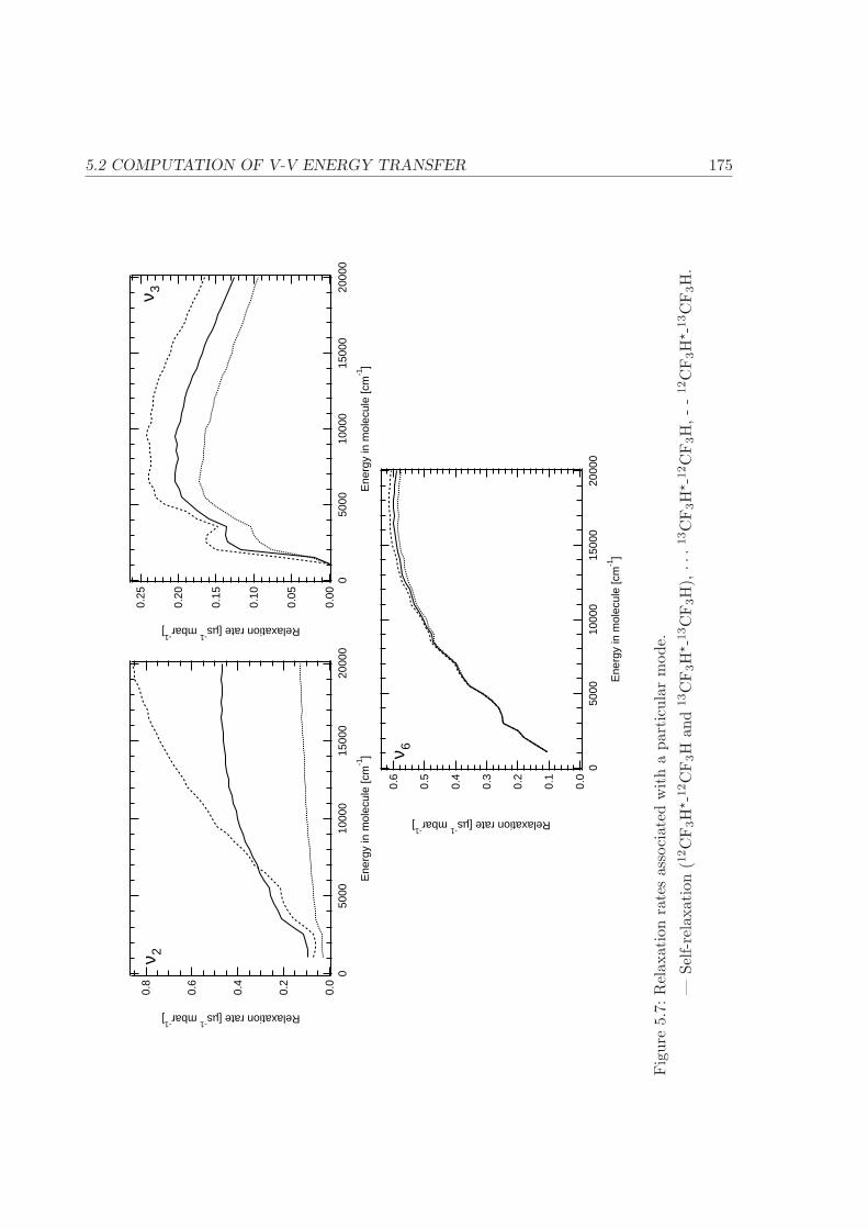
5.2 COMPUTATION OF V-V ENERGY TRANSFER 1750.
8
0.6
0.4
0.2
0.0
Relaxation rate [µs-1
mbar-1
]
2000
015
000
1000
050
000
Ene
rgy
in m
olec
ule
[cm
-1]
ν 20.
25
0.20
0.15
0.10
0.05
0.00
Relaxation rate [µs-1
mbar-1
]
2000
015
000
1000
050
000
Ene
rgy
in m
olec
ule
[cm
-1]
ν 3
0.6
0.5
0.4
0.3
0.2
0.1
0.0
Relaxation rate [µs-1
mbar-1
]
2000
015
000
1000
050
000
Ene
rgy
in m
olec
ule
[cm
-1]
ν 6
Fig
ure
5.7:
Rel
axat
ion
rate
sas
soci
ated
wit
ha
part
icul
arm
ode.
—Se
lf-re
laxa
tion
(12C
F3H
?-1
2C
F3H
and
13C
F3H
?-1
3C
F3H
),···1
3C
F3H
?-1
2C
F3H
,-
-12C
F3H
?-1
3C
F3H
.

176 CHAPTER 5. NUMERICAL SIMULATIONS
The figures 5.6 and 5.7 show different behaviours of the relaxation rates as a function
of the vibrational energy in the donor molecule. However, a general feature is that the
relaxation rate increases first, goes through a maximum and falls afterwards. This can
be understood as follows. The relaxation rate is defined by the overlap of the absorption
and the emission spectra of the donor and acceptor molecules, i.e. the shift between
the two spectra and their intensities (integral absorption/emission strength). The be-
haviour of the shift is illustrated in figure 5.8 for the example of an excited 12CF3H
molecule relaxing on a 13CF3H molecule in the ground state.
Abs
orpt
ion
/ em
issi
on
Frequency
Energy E2
of donor molecule
Energy E1
of donor molecule
Energy E0
of donor molecule
Figure 5.8: The shift between — absorption and - - emission spectra as a function of the energy
of the donor molecule (E0 < E1 < E2), using the example of 13CF3H as acceptor
molecule and 12CF3H as donor molecule.
In order to get a feeling for the behaviour of the relaxation rate as a function of the
vibrational energy E of the excited molecule we use the following approximate Gaus-
sian absorption spectrum Ar and emission spectrum Er (see section 5.1, using constant
widths ω of the absorption/emission spectra):

5.2 COMPUTATION OF V-V ENERGY TRANSFER 177
Ar ≈ exp(− (
ν−νa
ω
)2)
Er ≈ (1 + A · E) · exp
(−
(ν−(νd−E·∆ν)
ω
)2)
,(5.36)
where A and ∆ν are constants which depend on the vibrational modes we are con-
sidering (see table 5.1 on page 161) and νa and νd are the concerned band origins in
the vibrational ground state of the acceptor and donor molecules. In this case, the
vibrational relaxation rate W is given by
W ∝ ∫band
Ar(ν)Er(ν)dν
∝ (1 + A · E)︸ ︷︷ ︸(I)
· exp
(−1
2·(
(νd − νa)− E ·∆ν
ω
)2)
︸ ︷︷ ︸(II)
, (5.37)
The figure 5.9 shows this function using again the example of excited 12CF3H re-
laxing on ground state 13CF3H, using the ν5 vibration as mediating vibration (A =
2.08 · 10−4(cm−1)−1, ∆ν = −7.09 · 10−3(cm−1)−1 (table 5.1), νd − νa = 25 cm−1 and
ω ≈ 25 cm−1).
4
3
2
1
012000800040000
Energy in molecule [cm-1
]
1+A E, part (I)
Overlapp, part (II)
Total, (I) * (II)
Figure 5.9: Parts (I) and (II) of equation 5.37 and the total relaxation rate W .

178 CHAPTER 5. NUMERICAL SIMULATIONS
The solid curve in figure 5.9 can be compared with the dashed curve in figure 5.6 on
page 174. The differences are due to the fact that here we have only done an approxi-
mate calculation in order to get an intuitive understanding of the processes.
In this spirit the following observations can be done and understood regarding the
calculated relaxation rates given in figures 5.6 and 5.7.
1. In general the cross-relaxation of vibrationally excited 12CF3H on 13CF3H is faster
than self-relaxation, which itself is faster than the relaxation of excited 13CF3H on12CF3H in the ground state. For two molecules of the same isotopic species, the
absorption and emission spectra are shifted by the anharmonic shift due to the
vibrational excitation of the donor molecule (E ·∆ν 6= 0, νd = νa in equation 5.37).
In the case of relaxation between molecules of different isotopic species, there is
an additional isotopic shift (νd 6= νa). For excited 13CF3H relaxing on 12CF3H in
the ground state, these shifts have the same sign (νd − νa < 0, −E · ∆ν < 0),
thus decreasing the energy transfer rate. In the case of excited 12CF3H relaxing
on 13CF3H in the ground state, these shifts have opposite signs (νd − νa > 0,
−E · ∆ν < 0) canceling each other and this way increasing the energy transfer
rates.
2. The anharmonic red-shift of the absorption spectrum grows upon increasing the
level of vibrational excitation. In the case of self-relaxation and the relaxation of
excited 13CF3H on ground state 12CF3H this effect tends to decrease the overall
relaxation rate because the overlap of the emission spectrum with the ground state
absorption spectrum decreases. In the case of excited 12CF3H relaxing on ground
state 13CF3H this effect first tends to increase the relaxation rates because the
isotopic and the anharmonic shifts have opposite signs, such as the overall shift
reduces upon excitation. At some point the anharmonic shift prevails and the
overall shift begins to increase, resulting in a decrease of the relaxation rates (ν3
and ν5 are good examples).
3. In the case of the ν6 mode the isotopic shift is small (∼1 cm−1) compared with
the anharmonic one (νd ≈ νa in equation 5.37), such as the computed relaxation
rates are almost the same for all three pairs of isotopic species.

5.2 COMPUTATION OF V-V ENERGY TRANSFER 179
4. For strong anharmonic modes, the drop in V-V energy transfer rate at high ener-
gies is faster because the overlap of the emission spectrum and the ground state
absorption spectrum decreases faster (ν5 is very anharmonic whereas ν2 and ν6 are
only slightly anharmonic).
The resulting relaxation rates for the ν2, ν3, ν5 and ν6 modes can be added together to
get the total relaxation rate. It turns out that in most cases ν5 is by far the most impor-
tant mediating mode for V-V energy transfer, which is due to the very large transition
dipole moment. This shows a posteriori that leaving away ν1 and ν4 does not alter
the results significantly. In general, in the dipole-dipole model of collisional vibrational
energy transfer the most important contribution is to be expected from the vibrations
with a large transition dipole moment (ν5) and/or a low frequency‡ (ν6).
Figure 5.10 shows the contribution of the ν5 mode to the V-V energy transfer for self-
relaxation (12CF3H? - 12CF3H and 13CF3H
? - 13CF3H) and for cross-relaxation (12CF3H?
- 13CF3H and vice versa). For example, at vCH = 3, the contribution of ν5 lies between
90% (13CF3H? - 12CF3H) and 98% (12CF3H
? - 13CF3H).
The resulting relaxation rates will be dominated by ν5 and closely resemble the curves
for this mode which is presented in figure 5.6. We defined in equation 4.13 the following
values:
R12 := κ(12? − 13)/κ(12? − 12)
R13 := κ(13? − 13)/κ(13? − 12) ,(5.38)
where κ(x? − y) is the relaxation rate of excited xCF3H on ground state yCF3H. We
were able to measure R12 and R13 experimentally. Figure 5.11 shows the calculated
and the measured values for R12 and R13 as a function of the vibrational energy in the
excited molecule.
‡The transition strength between two states | v1, v2, . . . , vp, . . . , v6〉 → | v1, v2, . . . , vp − 1, . . . , v6〉 scales as
σ(vp → vp − 1) = vp · σ(1 → 0). This means that upon an increase of vibrational quantum numbers (i.e. with
increasing level of vibrational excitation) the transition strengths go up. In general, ν6 (ω6 ∼507 cm−1) has the
highest average occupation number, making this mode increasingly important for relaxation at high vibrational
levels.

180 CHAPTER 5. NUMERICAL SIMULATIONS
1.00
0.95
0.90
0.85
0.80
Con
trib
utio
n of
ν5
to V
-V E
.T.
20000150001000050000
Energy in molecule [cm-1
]
Selfrelaxation
Excited 13
CF3H on 12
CF3H
Excited 12
CF3H on 13
CF3H
Figure 5.10: Contribution of ν5 to the V-V energy transfer process.
5
4
3
2
1
0
Rx
20000150001000050000
Energy in molecule [cm-1
]
R12
R13
Figure 5.11: Results for • — R12 and - - R13 where only vibrational energy transfer via long
range dipole-dipole interactions are considered (• and : experimental data, —
and - -: numerical simulations).
The calculated values of R13 are nearly twice as high as the experimental values, overes-
5.2 COMPUTATION OF V-V ENERGY TRANSFER 181
timating the observed isotopic selectivity. Also the calculated values for R12 are slightly
overestimated. Apparently our simple model does not account for all details of the pro-
cess to make the results accurate. Although we do not attempt to elaborate a suitable
accurate model here, we discuss in the following section the most sensitive simplifica-
tions of our model and possible physical mechanisms, which are likely to be considered
in the initial stages of improving accuracy.
5.2.5 Discussion
Perhaps the most important result of our performed calculations in the framework of
a relatively simple model based only on dipole-dipole interactions is that there has
to be, indeed, a significant isotopic selectivity in collisional vibrational deactivation of
CF3H. The qualitative behaviour of this selectivity corresponds well to our experimental
observations. Nevertheless there is still a considerable quantitative discrepancy between
the calculations and the experiments (figure 5.11). Below we analyse in more detail
the assumptions of the model that we used in the previous section. The following
assumptions were used:
1. Rotational relaxation is complete.
2. IVR is complete.
3. Higher order poles do not contribute to V-V energy transfer. All encounters of
two molecules with a distance R < R0 are excluded. R0 is a cut-off distance where
higher order interaction terms prevail with respect to dipole-dipole interactions.
Assumption 1 is well met, since we do not detect any rotational dependence of isotopic
selectivity (see the experimental data in section 3.2), so this point will not be investi-
gated further.
Concerning the problem of IVR (assumption 2), we made the assumption IVR is com-
plete in the molecule undergoing vibrational energy transfer‡. Intrinsic IVR such as
collisionally induced IVR can occur. We have discussed this issue earlier: in CF3H
‡Vibrational energy transfer prior to IVR is possible, but very slow, because the emission spectrum of a
molecule in the 31 state overlaps very little with the absorption spectrum of a CF3H molecule in the ground
state.

182 CHAPTER 5. NUMERICAL SIMULATIONS
excited via the 31 mode the time-scale for collision-free IVR is on the 100 ps time-scale
(section 2.1.2.B) and for collision-induced IVR roughly 10-20 ns for a sample pressure of
1 mbar (section 2.1.2.C and using the relation the CI-IVR scales with the pre-excitation
energy16). Furthermore a single encounter of two molecules can potentially induce IVR
and then mediate V-V energy transfer in the same collision. It is hence reasonable to
assume that our second assumption is well met.
Assumption 3 is a rather strong simplification. In the last section we described our cal-
culations of vibrational energy transfer rates for CF3H assuming exclusively the dipole-
dipole interaction mechanism of the transfer. In reality, higher order interactions, like
quadrupole, may also be significant, especially at short intermolecular distances. It is
reasonable to expect that the isotopic selectivity of the energy transfer caused by these
short distance interactions is negligible. The rotational selection rules ∆J , ∆K = (0,)
± 1 are broken and scale with the order of the pole broadening the emission and absorp-
tion spectra. For very high order interactions this broadening scrambles any isotopic
selectivity. This non-selective transfer via multipole interactions would offset the iso-
topically selective transfer rates, calculated for dipole-dipole interactions, approaching
the overall calculated isotopic selectivity to the experimentally measured values.
In what follows we take into account these higher order poles in such “head-on” colli-
sions. Although in principle we could treat the process in a similar manner as we did for
dipole-dipole interactions, it is practically not feasible, as no information on quadrupole,
let alone higher order poles exist for this molecule. We hence empirically summarise
the set of higher order poles into one single parameter: the number of collisions ℵ with
a mutual distance ≤ R0 it takes for a molecule to lose the same amount of energy as by
resonant energy transfer (via the ν5 vibration, i.e. ∼1000 cm−1). We are now left with
two parameters: R0 and ℵ, which have to be varied to adequately fit our experimental
data. For the vibrational energy transfer rate for large distance encounters R ≥ R0 we
use the transition rates calculated previously. We use two fitting parameters, R0 and ℵ,
because we want to reproduce both the isotopic selectivity for the relaxation rates and
their absolute values. Note that we have two values, R12 = κ(12?−12)/κ(12?−13) and
R13 = κ(13? − 12)/κ(13? − 13), for four different pre-excitation levels we would like to
reproduce with only two fitting parameters.
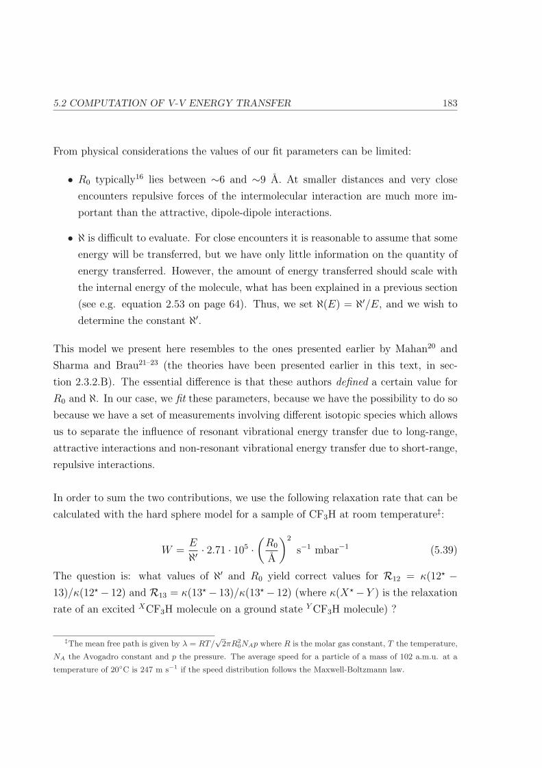
5.2 COMPUTATION OF V-V ENERGY TRANSFER 183
From physical considerations the values of our fit parameters can be limited:
• R0 typically16 lies between ∼6 and ∼9 A. At smaller distances and very close
encounters repulsive forces of the intermolecular interaction are much more im-
portant than the attractive, dipole-dipole interactions.
• ℵ is difficult to evaluate. For close encounters it is reasonable to assume that some
energy will be transferred, but we have only little information on the quantity of
energy transferred. However, the amount of energy transferred should scale with
the internal energy of the molecule, what has been explained in a previous section
(see e.g. equation 2.53 on page 64). Thus, we set ℵ(E) = ℵ′/E, and we wish to
determine the constant ℵ′.
This model we present here resembles to the ones presented earlier by Mahan20 and
Sharma and Brau21–23 (the theories have been presented earlier in this text, in sec-
tion 2.3.2.B). The essential difference is that these authors defined a certain value for
R0 and ℵ. In our case, we fit these parameters, because we have the possibility to do so
because we have a set of measurements involving different isotopic species which allows
us to separate the influence of resonant vibrational energy transfer due to long-range,
attractive interactions and non-resonant vibrational energy transfer due to short-range,
repulsive interactions.
In order to sum the two contributions, we use the following relaxation rate that can be
calculated with the hard sphere model for a sample of CF3H at room temperature‡:
W =E
ℵ′ · 2.71 · 105 ·(
R0
A
)2
s−1 mbar−1 (5.39)
The question is: what values of ℵ′ and R0 yield correct values for R12 = κ(12? −13)/κ(12?− 12) and R13 = κ(13?− 13)/κ(13?− 12) (where κ(X?− Y ) is the relaxation
rate of an excited XCF3H molecule on a ground state Y CF3H molecule) ?
‡The mean free path is given by λ = RT/√
2πR20NAp where R is the molar gas constant, T the temperature,
NA the Avogadro constant and p the pressure. The average speed for a particle of a mass of 102 a.m.u. at a
temperature of 20C is 247 m s−1 if the speed distribution follows the Maxwell-Boltzmann law.
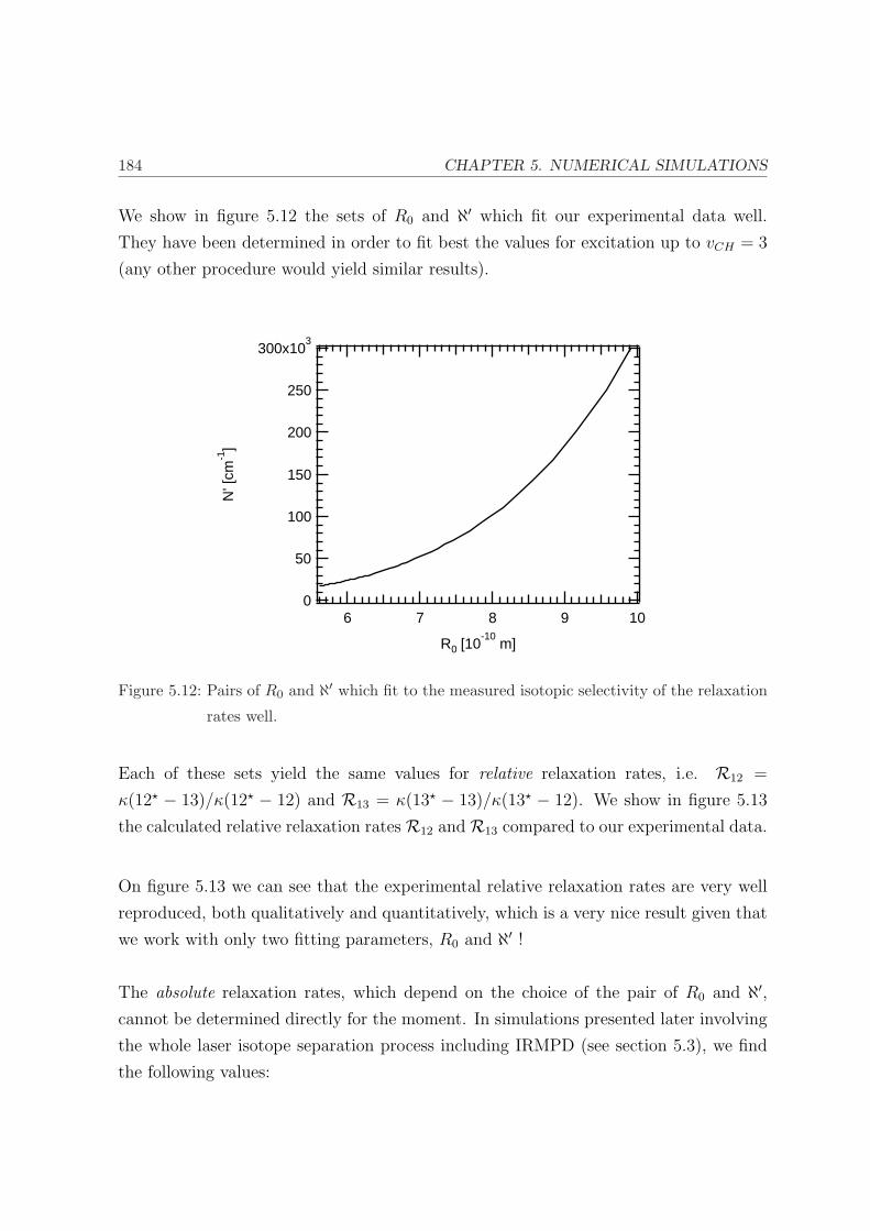
184 CHAPTER 5. NUMERICAL SIMULATIONS
We show in figure 5.12 the sets of R0 and ℵ′ which fit our experimental data well.
They have been determined in order to fit best the values for excitation up to vCH = 3
(any other procedure would yield similar results).
300x103
250
200
150
100
50
0
N' [
cm-1
]
109876
R0 [10-10
m]
Figure 5.12: Pairs of R0 and ℵ′ which fit to the measured isotopic selectivity of the relaxation
rates well.
Each of these sets yield the same values for relative relaxation rates, i.e. R12 =
κ(12? − 13)/κ(12? − 12) and R13 = κ(13? − 13)/κ(13? − 12). We show in figure 5.13
the calculated relative relaxation rates R12 and R13 compared to our experimental data.
On figure 5.13 we can see that the experimental relative relaxation rates are very well
reproduced, both qualitatively and quantitatively, which is a very nice result given that
we work with only two fitting parameters, R0 and ℵ′ !
The absolute relaxation rates, which depend on the choice of the pair of R0 and ℵ′,cannot be determined directly for the moment. In simulations presented later involving
the whole laser isotope separation process including IRMPD (see section 5.3), we find
the following values:
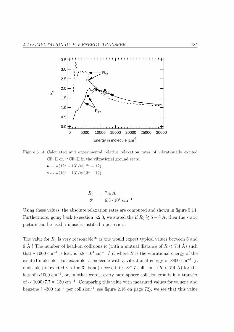
5.2 COMPUTATION OF V-V ENERGY TRANSFER 185
3.5
3.0
2.5
2.0
1.5
1.0
0.5
0.0
Rx
300002500020000150001000050000
Energy in molecule [cm-1
]
R12
R13
Figure 5.13: Calculated and experimental relative relaxation rates of vibrationally excited
CF3H on 12CF3H in the vibrational ground state.
• — κ(12? − 13)/κ(12? − 12).
- - κ(13? − 13)/κ(13? − 12).
R0 = 7.4 A
ℵ′ = 6.8 · 104 cm−1
Using these values, the absolute relaxation rates are computed and shown in figure 5.14.
Furthermore, going back to section 5.2.3, we stated the if R0 & 5− 8 A, then the static
picture can be used, its use is justified a posteriori.
The value for R0 is very reasonable16 as one would expect typical values between 6 and
9 A ! The number of head-on collisions ℵ (with a mutual distance of R < 7.4 A) such
that ∼1000 cm−1 is lost, is 6.8 · 104 cm−1 / E where E is the vibrational energy of the
excited molecule. For example, a molecule with a vibrational energy of 8800 cm−1 (a
molecule pre-excited via the 31 band) necessitates ∼7.7 collisions (R < 7.4 A) for the
loss of ∼1000 cm−1, or, in other words, every hard-sphere collision results in a transfer
of ∼ 1000/7.7 ≈ 130 cm−1. Comparing this value with measured values for toluene and
benzene (∼300 cm−1 per collision24, see figure 2.16 on page 72), we see that this value

186 CHAPTER 5. NUMERICAL SIMULATIONS
12
10
8
6
4
2
0
Rel
axat
ion
rate
[µs-1
mba
r-1]
300002500020000150001000050000
Energy in molecule [cm-1
]
Figure 5.14: Relaxation rates as a function of the energy in the molecule (for R′0 = 7.4 A,
ℵ′ = 6.8 · 104 cm−1).
— self-relaxation rates
· · · excited 13CF3H on ground state 12CF3H
- - excited 12CF3H on ground state 13CF3H
has the correct order of magnitude.
5.2.6 Conclusions
In this section we have described how we calculate collisional relaxation rates of excited
CF3H molecules on ground state CF3H molecules. Under certain assumptions described
at the beginning, we develop a theory for the calculation of relaxation rates for VET
mediated by dipole-dipole interactions. We show that if we consider only these long-
range interactions the calculated isotopic selectivity is too high, and we show that we
necessitate non-selective collisional relaxation by head-on collisions in order to repro-
duce the experimental values of isotopic selectivity. The dependency of this selectivity
on the vibrational energy of a molecule is very well reproduced (figure 5.13).
We have given a coherent picture of the process of the exchange of one quantum during
the collision between an excited and a ground state CF3H molecule. We have shown
5.3 NUMERICAL SIMULATIONS OF IRMPD IN THE PRESENCE OF COLLISIONS 187
that with a simple model we can correctly describe the experimentally observed isotopic
selectivity. In particular, we have shown that for encounters between two molecules with
an impact parameter & 7.4 A, near-resonant V-V energy transfer occurs and that for
smaller mutual distances non-resonant V-V’,T,R energy transfer occurs.
5.3 Numerical simulations of IRMPD in the presence of colli-
sions
In this section we present numerical simulations of our molecular laser isotope separation
(MLIS) process consisting of pre-exciting molecules to a vibrational overtone of the CH
stretch-bend vibration, and then selectively dissociating only pre-excited molecules. The
goal is twofold: first, we seek a better understanding of how different parameters affect
our MLIS process and secondly we interested which mechanisms lead to the increase of
isotopic selectivity upon an increase of the sample pressure. For this, these simulations
are necessary as the IRMPD is a non-linear process with respect to the fluence of the
CO2 dissociation laser, which has been well confirmed by experiments and simulations
before25, 26. After a brief introduction to the subject, we briefly state the equations that
have to be solved by the numerical code. Then we show how to evaluation the physical
parameters of these equations. We finally present the results: here, we first compare
our simulations with our experimental data and show that our model reliably describes
the processes. This allows us to have a look at the mechanisms of and the influences of
different physical parameters on our MLIS scheme.
5.3.1 Generalities
In our approach to the numerical simulations, we base ourselves on a statistical treat-
ment presented earlier in this text (see section 2.2.3.B). Briefly, one bins the vibrational
levels into coarse grained levels of width ∆E, i.e. all vibrational states with an energy
E lying between i∆E and (i + 1)∆E belong to level i. This way one uses calculated
transition rates for the population and depopulation of these bins . These transition
rates are calculated averaging over all possible transitions between the members of the
bins.
188 CHAPTER 5. NUMERICAL SIMULATIONS
For the simulation of the whole MLIS process, we take these grained energy levels
as a starting point, taking into account the following effects by which the molecule may
lose or gain energy:
IR photon absorption/emission: by absorbing or emitting one quantum of energy
p∆E molecules are pumped up and down.
Unimolecular dissociation: if the molecules have enough energy, they can dissociate.
For CF3H the lowest dissociation channel is CF3H→ CF2 + HF.
Collisions: in collisions molecules can undergo vibrational relaxation and gain or lose
energy.
Overtone pre-excitation: for the MLIS experiments a part of the molecules are pro-
moted with a laser via an overtone of the CH stretch vibration into a vibrationally
excited state.
In principle spontaneous emission could be included too, but it can be safely neglected27
because the time-scale for such a process is typically milliseconds whereas we are work-
ing on time-scales of 100 ns - 1 µs. We show in figure 5.15 the main effects by which
the molecules can gain or lose vibrational energy.
For all our calculations the ensemble of molecules is considered to be rotationally re-
laxed (in section 3.2 we have shown that at a pressure of & 1 mbar rotational relaxation
is complete). In principle uncomplete rotational relaxation could be treated by intro-
ducing some phenomenological parameters into the dissociation laser absorption steps
characterising the degree of rotational relaxation28, but as we work at pressures of typ-
ically ∼1 mbar this problem is circumvented.
5.3.2 Formalisation of the problem: the master equation
For the numerical simulations we work with a large ensemble of molecules, each one
having a certain internal energy E lying in a certain bin i. Ni is defined as the proba-
bility of a molecule having an energy corresponding to bin i and is a function of time.
We have to consider only the first n bins, where n has to be large enough so that for the
highest lying bin dissociation is very important compared to up- and down-pumping by

5.3 NUMERICAL SIMULATIONS OF IRMPD IN THE PRESENCE OF COLLISIONS 189
Figure 5.15: Energy level diagram: ↑ and ↓ are due to collisions; ⇑ and ⇓ are due to pumping
by the CO2 laser; 99K are losses due to unimolecular dissociation of the molecules.
The pre-excitation step is not shown.
the laser or by collisions.
We define
190 CHAPTER 5. NUMERICAL SIMULATIONS
N :=
N0
N1
N2
...
Nn−1
(5.40)
and the goal is to find equations describing the variation of N as a function of time.
CO2 laser pumping: The CO2 laser photons make steps of p. The population and
depopulation rates of the grained bins read
dNi
dt= − (
IRki+p,i + IRki−p,i
) ·Ni + IRki,i−p ·Ni−p + IRki,i+p ·Ni+p, (5.41)
where IRki±p,i are the up- and down-pumping constants from level i to levels i±p.
Dissociation: Rates due to unimolecular dissociation read
dNi
dt= − dki ·Ni, (5.42)
where dki is the dissociation rate of level i.
Collisions: Define ckijkl as rate of vibrational energy transfer via
M1(i) + M2(j)ckijkl−−−→ M1(k) + M2(l) (+∆E) , (5.43)
where i, j, k, l are the labels of the energy bins of molecules 1 and 2. In that case,
the rate equations read
dNi
dt= −
n−1∑j=0
ckij ·Ni ·Nj +n−1∑j1=0
n−1∑j2=0
ckj1j2i ·Nj1 ·Nj2 , (5.44)
where
ckijk :=n−1∑l=0
ckijkl
ckij :=n−1∑k=0
n−1∑l=0
ckijkl .(5.45)

5.3 NUMERICAL SIMULATIONS OF IRMPD IN THE PRESENCE OF COLLISIONS 191
Overtone pre-excitation: The rates due to the pre-excitation laser read
dN0
dt= −pk ·N0
dNP
dt= pk ·N0 ,
(5.46)
where level p is the level populated by the pre-excitation laser.
Note that IRkij and pk are time dependent.
This leaves us with the following master equation
dNdt
= A1N + A2N 2, (5.47)
where A1 is a (n · n) matrix and A2 is a (n · n · n) tensor. Their elements are
(A1)ij =
−(dki +IR ki,i+p +IR ki,i−p) (i = j)IRki,j (i = j ± p)
0 (otherwise)
+
−pk (i = j = 0)pk (i = P, j = 0)
0 (otherwise)
(5.48)
and‡
(A2)ijk = ckjki − δij · ckik. (5.49)
In order to simplify the equation to be solved, we assume the following:
• The large majority of the molecules are in the ground state.
• Vibrational relaxation leads to steps of p between different bins (because it is
mainly mediated by one vibration, ν5 in our case).
The first condition is well satisfied in our experiments. This allows for the following
simplification: as ∀t : N0(t) ≈ 1 and Ni(t) ¿ 1(∀t, ∀i > 1) the relaxation rates can be
embedded into A1. Secondly, only steps of p are done for vibrational relaxation: the
excited molecule moves down by p bins, the ground state molecules move up by p bins.
This way, the rates due to vibrational relaxation read:
‡(A2N 2)
k= ((A2N )N )k =
n−1∑i=0
n−1∑j=0
(A2)kij NiNj

192 CHAPTER 5. NUMERICAL SIMULATIONS
dN0
dt= vkj ·Np − F ·
n−1∑j=1
vkj ·Nj
dNi
dt= − vki ·Ni + vki+p ·Ni+p (i ≥ 1, i 6= p)
dNp
dt=
(F ·
n−1∑j=1
vkj ·Nj
)− vkp ·Np + vk2p ·N2p ,
(5.50)
where vkj is the relaxation rate of an excited molecule in bin j on ground state 12CF3H
and F is the 0.99 for the 12CF3H molecule and 0.01 for the 13CF3H molecule, taking into
account that there are also other relaxation partners in the sample other than the ones
we are considering in the simulations. The implementation into A1 is straightforward
and analogous to the previously explained cases. We are left with the following simplified
master equation
dN (t)
dt= A1(t) · N (t) (5.51)
to be solved by a numerical code.
5.3.3 Evaluation of physical values for the master equation
In the previous section we gave the master equation in expression 5.51. The (n·n) matrix
contains all rate constants that take into account the population and depopulation
due to the pre-excitation and the dissociation lasers, unimolecular dissociation and V-
V energy transfer. In the following sections we go into further detail regarding the
numerical evaluation of the different terms of A1.
5.3.3.A Overtone pre-excitation
Here the absolute values are not important. It has to be evaluated in such a way that a
small fraction of the molecules are pre-excited (typically ∼1-5%) in order to fulfill the
assumption that relaxation occurs only on molecules in the vibrational ground state.
5.3.3.B Collisional relaxation
In section 5.2 we have calculated the relative relaxation rates, the absolute values are
not known. We take the rates for collisional relaxation determined numerically (in

5.3 NUMERICAL SIMULATIONS OF IRMPD IN THE PRESENCE OF COLLISIONS 193
section 5.2) and introduce a scaling parameter that has to be fitted in our simulations.
5.3.3.C Unimolecular dissociation
In the absence of any experimental data the dissociation rates of molecules excited above
the dissociation limit have to be calculated. The central equation for calculating the
dissociation rate k(E) is
k(E) =N ‡(E − E0)
hρ(E), (5.52)
where N ‡ is the sum of states at the transition state, where the reaction coordinate
remains fixed, ρ is the reactant density of states, E is the energy inside the molecule
and E0 is the energy at the transition state with respect to the ground state of the
reactant. To apply this the existence of a transition state is a pre-requisite. This is
a (unique) saddle point on the potential energy surface that the molecule necessarily
has to cross to dissociate and which separates the bound state from the dissociated state.
Different theories for the calculation of dissociation rates commonly admit equation 5.52,
they differ in how N ‡ and ρ are evaluated. Popular theories include RRK and RRKM29,
SACM30 (Statistical adiabatic channel model) or phase space theories (PST). We use
the RRKM theory.
In the RRK (Rice-Ramsperger-Kassel) theory31–33 the molecule is treated as a set of s
independent harmonic oscillators which, however, freely exchange energy. This energy is
statistically distributed over all vibrational degrees of freedom. Within this framework
the evaluation of N ‡ and ρ is done by direct counting (including anharmonicity). The
calculations are very straightforward, although some knowledge of the transition state
(energy E0 and vibrational frequencies) is necessary. In the RRKM (RRK-Marcus) the-
ory34–37 the effect of rotational energy, angular momentum and zero-point energies are
explicitly included.
(I) RRKM calculations for CF3H
The unimolecular dissociation reaction of CF3H has different channels, the three lowest
194 CHAPTER 5. NUMERICAL SIMULATIONS
are38
CF3H → CF2 + HF (∼ 20, 500cm−1)
CF3H → CF3 + H (∼ 37, 250cm−1)
CF3H → CF2H + F (∼ 45, 000cm−1)
where the energies in brackets are evaluated by Shin38 calculating the differences of the
enthalpy Hf of CF3H and the products39. The dissociation level can lie higher if they
go through an energetic maximum. In the case of the first dissociation channel, it lies
at40 ∼24,000 cm−1.
For the calculation of the dissociation rates we use the dissociation energy ETS and
the vibrational frequencies ωTSi at the transition state computed by Shin38 as shown in
table 5.2.
ETS / cm−1 25,880
ωTSi / cm−1 2204, 1259, 1180, 1096, 877, 597, 302, 223
Table 5.2: Energy and vibrational frequencies at the transition state for the lowest dissociation
channel CF3H→ CF2 + HF
For the RRK calculations we employ a code written in the group of Martin Quack.
The dissociation rates can be compared with experimental data as follows. Several
studies of dissociation rates as a function of the temperature exist, and the conversion
for energy dependent dissociation rates k(E) to temperature dependent dissociation
rates k(T ) is done with via the relation
k(T ) =
∫k(E)p(E, T )dE, (5.53)
where p(E, T ) is the Maxwell Boltzmann distribution at a temperature T .
Figure 5.16 shows the temperature dependence of CF3H dissociation measured by dif-
ferent authors40–44 and the rates we get using our energy dependent dissociation rates
calculated with RRKM. One set of experimental data presented in the graph (dotted

5.3 NUMERICAL SIMULATIONS OF IRMPD IN THE PRESENCE OF COLLISIONS 195
line) lies quite far away from the others; furthermore these measured dissociation rates
lie very high with respect to typical dissociation rates for the transition considered45,
so we can suppose that the latest of the three other measurements is the most reliable.
It coincides well with our calculations.
10-2
10
0
10
2
10
4
10
6
10
8
k [s
-1]
220020001800160014001200
Temperature [K]
Tschuikow 1965 Modica 1966 Schug 1979 Hidaka 1991 Own by RRKM
Figure 5.16: Arrhenius plots of experimental data for CF3H measured by different authors.
For these reasons, we take our computed dissociation rates without any further modifi-
cations‡.
(II) Isotopic influences on unimolecular dissociation
Unimolecular dissociation itself is isotopically selective due to two effects29, 46, 47: there
is a critical energy effect and a statistical weight effect. The first effect is due to a
different zero point energy for different molecular isotopic species which makes the dis-
sociation energy different. The second effect is that different density of states ρ due to
different vibrational energies give different unimolecular dissociation rates.
‡The exact values for the dissociation rates are not crucial for the calculation of the final dissociation yield
of an IRMPD experiment45.
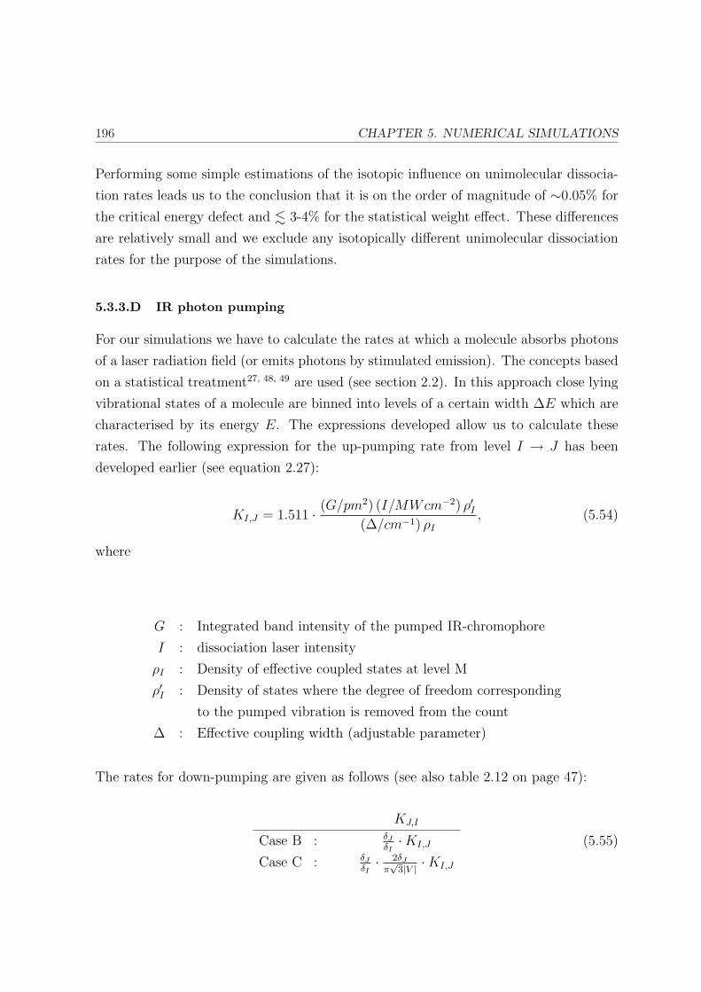
196 CHAPTER 5. NUMERICAL SIMULATIONS
Performing some simple estimations of the isotopic influence on unimolecular dissocia-
tion rates leads us to the conclusion that it is on the order of magnitude of ∼0.05% for
the critical energy defect and . 3-4% for the statistical weight effect. These differences
are relatively small and we exclude any isotopically different unimolecular dissociation
rates for the purpose of the simulations.
5.3.3.D IR photon pumping
For our simulations we have to calculate the rates at which a molecule absorbs photons
of a laser radiation field (or emits photons by stimulated emission). The concepts based
on a statistical treatment27, 48, 49 are used (see section 2.2). In this approach close lying
vibrational states of a molecule are binned into levels of a certain width ∆E which are
characterised by its energy E. The expressions developed allow us to calculate these
rates. The following expression for the up-pumping rate from level I → J has been
developed earlier (see equation 2.27):
KI,J = 1.511 · (G/pm2) (I/MWcm−2) ρ′I(∆/cm−1) ρI
, (5.54)
where
G : Integrated band intensity of the pumped IR-chromophore
I : dissociation laser intensity
ρI : Density of effective coupled states at level M
ρ′I : Density of states where the degree of freedom corresponding
to the pumped vibration is removed from the count
∆ : Effective coupling width (adjustable parameter)
The rates for down-pumping are given as follows (see also table 2.12 on page 47):
KJ,I
Case B : δJ
δI·KI,J
Case C : δJ
δI· 2δJ
π√
3|V | ·KI,J
(5.55)

5.3 NUMERICAL SIMULATIONS OF IRMPD IN THE PRESENCE OF COLLISIONS 197
where δX is the the average spacing between the vibrational states in bin X, and |V | is
the average coupling between the states in the upper and lower bin via the laser radia-
tion. The “Case B” refers to regions of high density of states, where the states within a
grained level are all coupled amongst each other, and “Case C” refers to regions of low
density of states, where the states within a grained level are uncoupled amongst each
others, and couple only via the laser radiation to levels in the other bin.
We would like to introduce two generalisations, which are presented in this section:
1. Equations 5.54 and 5.55 give the expressions for the up and down-pumping rates
of excited molecules. In particular, we give values for the case of pumping through
regions of low densities of states (the “case C”). These results however are ex-
plicitly given using the assumption that the upper level is and stays essentially
unpopulated compared to the lower level during the whole experiment. This con-
dition is reasonably well met for the calculation of IRMPD of molecules in the
ground state. However, in our simulations, where we pre-excite molecules to a
certain level and then also pump them down by the CO2 laser, we have the inverse
situation. This necessitates a certain generalisation of the formulae. We show in
appendix A how the pumping rates are developed, and we show also that a direct
generalisation is not possible in the framework of our master equations presented
here. We propose the following pragmatic solution: for each couple of bins between
which molecules can be pumped up and down, we first determine which of the two
states is more populated. If this is the lower state, we use the pumping rates as
described in equation 5.55. In the opposite case, the calculation of the pumping
rates is inverted. The general statement of pumping through low density of states
is: “Up-pumping through a low density region is slow”. We would like to add: “...
down-pumping too !”.
2. A second and very important improvement is to introduce a dependence of the
pumping-rates on the isotopic species and the vibrational energy of the molecule
and the wavelength of the pumping laser. The value of G/∆ in equation 5.54
gives the absorption cross-section and is an average over multiple absorption steps
(figure 5.17-I). We propose generalising equation 5.54 by replacing G/∆ by a cal-
culated absorption cross-section which depends on the laser frequency ν, the vi-
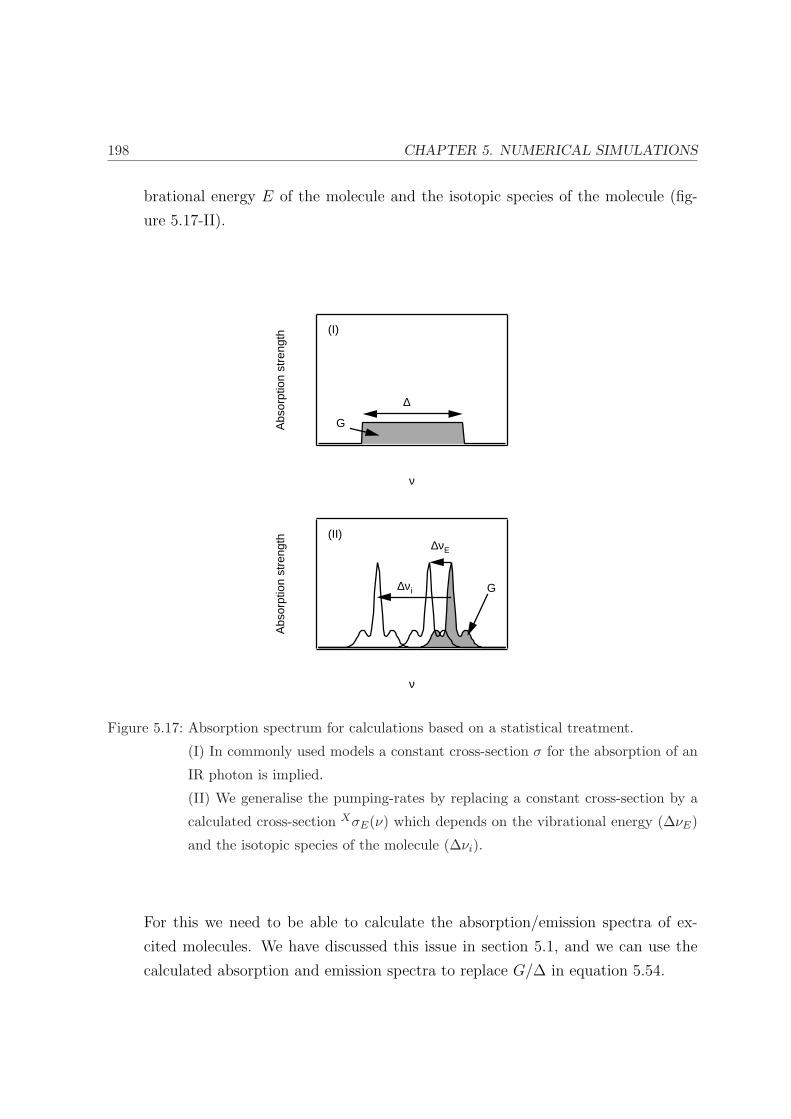
198 CHAPTER 5. NUMERICAL SIMULATIONS
brational energy E of the molecule and the isotopic species of the molecule (fig-
ure 5.17-II).
Abs
orpt
ion
stre
ngth
ν
G
(II)∆νE
∆νi
Abs
orpt
ion
stre
ngth
ν
∆
G
(I)
Figure 5.17: Absorption spectrum for calculations based on a statistical treatment.
(I) In commonly used models a constant cross-section σ for the absorption of an
IR photon is implied.
(II) We generalise the pumping-rates by replacing a constant cross-section by a
calculated cross-section XσE(ν) which depends on the vibrational energy (∆νE)
and the isotopic species of the molecule (∆νi).
For this we need to be able to calculate the absorption/emission spectra of ex-
cited molecules. We have discussed this issue in section 5.1, and we can use the
calculated absorption and emission spectra to replace G/∆ in equation 5.54.

5.3 NUMERICAL SIMULATIONS OF IRMPD IN THE PRESENCE OF COLLISIONS 199
5.3.4 Results
5.3.4.A Some characteristics of the numerical code
Our numerical code is written in fortran 90 and contains roughly a thousand lines. It
is compiled on a PC with Plato v 2.11c from Salford Software, UK. The code can be
found in appendix E.
Basically, the code solves the master equation given in expression 5.51, which reads
dN (t)
dt= A(t) · N (t), (5.56)
where N is a vector with n elements containing the populations of the individual levels
and A(t) is a (n ·n) matrix incorporating all pumping, relaxation and dissociation rates.
To solve this, the code uses the fourth order Runge-Kutta50 method, advancing by steps
∆t in time. Each step is calculated twice, once advancing using a step ∆t, once using
two steps of ∆t/2. If the two results are the same within some given maximum error, the
step is accepted. Otherwise, the code redefines ∆t 7→ ∆t/2 and redoes the particular
step. This procedure is repeated until the results converge. For this reason, the time
steps can change within one simulation. A typical value for a starting point for ∆t is 2 ns.
For convenience a vibrational energy Ed is defined above which all molecules disso-
ciate rapidly and can never be pumped or relaxed down to the ground state. Typically,
we define Ed = 28,000 cm−1.
A single run simulates a three laser experiment, i.e. with pre-excitation, dissociation
and LIF lasers. It calculates the evolution of N for both isotopic species simultaneously.
The LIF laser is taken into account by stopping the simulations at the time when this
LIF laser intervenes and evaluating the number of dissociated molecules. The following
physical parameters can be chosen as input:
• Fluence of the dissociation laser
• Wavelength of the dissociation laser
• Pressure of sample

200 CHAPTER 5. NUMERICAL SIMULATIONS
• Pre-excitation energy
• Timing of lasers (pre-excitation∆tPE−IRMPD−−−−−−−−→ dissociation
∆tIRMPD−LIF−−−−−−−−−→ LIF)
The temporal shapes of the pre-excitation and dissociation lasers, the unimolecular dis-
sociation rates and the relaxation rates are given in separate input files. Optionally,
an experiment can be run twice, once with and once without pre-excitation, in order
to evaluate how much of the dissociated molecules are due to ground state dissocia-
tion (analogous to our experimental setup). There are some other input parameters
concerning the calculation procedure itself, such as some convergence criteria for the
calculations, the size of the energy bins, and so on. Typically, for rough calculations
bins of 1000 cm−1 are used. For the results presented in this text, we use bins of 200
cm−1.
The code stores the number of dissociated molecules in a single experiment in a file.
Optionally it can also store the number of dissociated molecules and the distribution
of vibrational energies of the molecules as a function of time. Figure 5.18 shows an
example of the number of dissociated molecules as a function of time, and figures 5.19
and 5.20 the distribution of the molecules at different moments for the same experiment.
The time for the calculation of a single three laser experiment varies as a function of the
parameters chosen, in particular the size of a bin. Typically, for calculations shown in
this document, half a minute is spent on a calculation of a single IRLAPS experiment
by a standard laptop (1.5 GHz, Intel Centrino) running Windows XP.
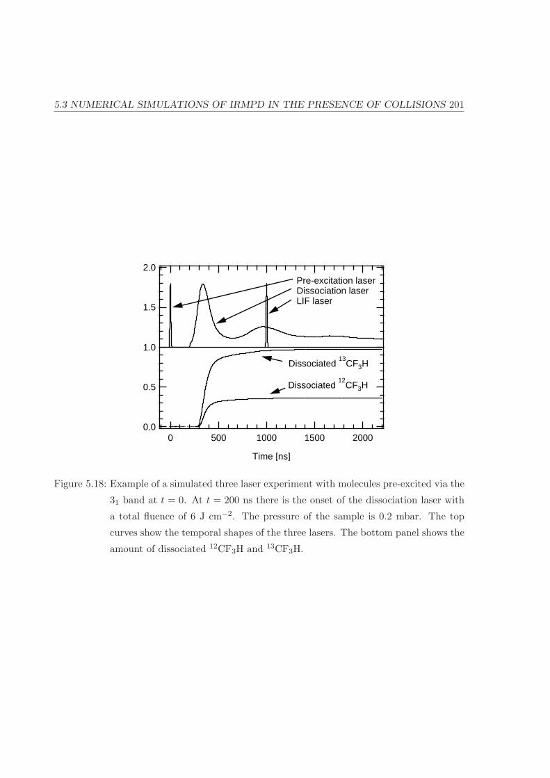
5.3 NUMERICAL SIMULATIONS OF IRMPD IN THE PRESENCE OF COLLISIONS 201
2.0
1.5
1.0
0.5
0.02000150010005000
Time [ns]
Dissociated 13
CF3H
Dissociated 12
CF3H
Pre-excitation laserDissociation laserLIF laser
Figure 5.18: Example of a simulated three laser experiment with molecules pre-excited via the
31 band at t = 0. At t = 200 ns there is the onset of the dissociation laser with
a total fluence of 6 J cm−2. The pressure of the sample is 0.2 mbar. The top
curves show the temporal shapes of the three lasers. The bottom panel shows the
amount of dissociated 12CF3H and 13CF3H.

202 CHAPTER 5. NUMERICAL SIMULATIONS
30000
25000
20000
15000
10000
5000
0
Vib
ratio
nal e
nerg
y [c
m-1
]
5x10⁻³
0
Population
30000
25000
20000
15000
10000
5000
0
Vib
ratio
nal e
nerg
y [c
m-1
]
10x10-3
0
Population
Figure 5.19: Energy distributions for the example shown in figure 5.18, for the 13CF3H iso-
topomer. The population in the ground state is cut away for clarity.
I Left graph, from left to right: t = 0, 100 and 200 ns (vibrational relaxation).
I Right graph, from left to right: t = 200, 220, 240, 250, 260, 300, 500, 1000 ns
(IRMPD).
The different curves have different offsets for clarity. Binwidths of ν0/5 have been
chosen (where ν0 = 1048 cm−1 is the frequency of the CO2 dissociation laser).
Through absorption or emission of a photon such as vibrational relaxation, only
steps of 5 bins are done, which explains why the population distribution goes
back to 0 in four out of five bins.

5.3 NUMERICAL SIMULATIONS OF IRMPD IN THE PRESENCE OF COLLISIONS 203
30000
25000
20000
15000
10000
5000
0
Vib
ratio
nal e
nerg
y [c
m-1
]
400x10-6
2000
Population
t = 1000 ns
x20
30000
25000
20000
15000
10000
5000
0
Vib
ratio
nal e
nerg
y [c
m-1
]
20x10-3
100
Population
t = 0 ns
30000
25000
20000
15000
10000
5000
0
Vib
ratio
nal e
nerg
y [c
m-1
]
10x10-3
50
Population
t = 200 ns
Figure 5.20: Dynamics of energy level populations calculated for CF3H (left curve on a graph:12CF3H, right curve on a graph: 13CF3H), at t = 0, 200 and t = 1000 ns for the
same experimental conditions as in figures 5.18 and 5.19. The curves for 13CF3H
are offset for clarity. At t = 0, the molecules are pre-excited at an energy of 8800
cm−1 (left graph). On the graph in the centre isotopically selective collisional
relaxation is put to evidence, in the right graph the higher pumping efficiency
for the 13CF3H isotopomer. Note that in the case of 12CF3H the population
at ∼1000 cm−1 is rapidly populated due to the warming up of molecules in the
ground state by collisions with excited molecules.
204 CHAPTER 5. NUMERICAL SIMULATIONS
5.3.4.B Comparison with experiments
In this section we present some comparisons between our experimental data and our
simulations. We also compare our simulations with data reported elsewhere51, 52. In
particular we compare our simulations with data presented in sections 4.3 (photofrag-
ment excitation spectra of vibrationally excited molecules and dissociation selectivity
at low pressures), 4.4 (Measurements of the decay rates as a function of the dissociation
laser fluence and frequency). The simulations have only a single fitting parameter: a
multiplicative constant for collisional relaxation, all other parameters are kept fixed.
Sections (I) and (II) concern the collision-free situations, and we show that our simula-
tions represent the experimental data well. In section (III) we present calculations with
which we can scale vibrational relaxation rates, and we finally present in section (IV)
simulations including the scaled vibrational relaxation rates.
(I) Simulation of photofragment spectra
To begin with, we present comparisons of the measured and calculated photofragment
spectra for molecules pre-excited via the 31 band. In these experiments we measured
the total dissociation probability D as a function of the frequency and the fluence of
the dissociation laser, always keeping a zero time-delay between the pre-excitation and
the dissociation lasers. For convenience, we describe the photofragment spectrum by
the function 4.1, which reads
D(ν) = 1− exp
(−B · exp
(−
(ν − ν0
ω
)2))
, (5.57)
where D is the dissociation probability, ν is the frequency of the dissociation laser, and
B, ν0 and ω are fitting parameters.
At the first step, we show simulated and measured dissociation yields at a particu-
lar dissociation laser frequency, as a function of the fluence of the dissociation laser.
Two examples, for dissociation laser frequencies of 1083 cm−1 and 977 cm−1 are shown
in figure 5.21 for the dissociation of 13CF3H.

5.3 NUMERICAL SIMULATIONS OF IRMPD IN THE PRESENCE OF COLLISIONS 205
1.0
0.8
0.6
0.4
0.2
0.0
Dis
soci
atio
n pr
obab
ility
12840
Dissociation laser fluence [J cm-2
]
(a) νdiss = 1083 cm−1 (13CF3H)
1.0
0.8
0.6
0.4
0.2
0.0
Dis
soci
atio
n pr
obab
ility
20151050
Dissociation laser fluence [J cm-2
]
(b) νdiss = 977 cm−1 (13CF3H)
Figure 5.21: — Simulated and • measured dissociation yields.
Considering that the experiments are performed at 0.4 mbar, where rotational relax-
ation is not complete, we cannot compare the experiments and the simulated values
directly. For a pressure of 1 mbar, where rotational relaxation is more complete, the
dissociation probability is larger. Experimentally we have determined that at a disso-
ciation laser fluence of ∼ 3 J cm−2 and a pressure of 0.4 mbar the dissociation yield
is ∼50% of what it would be if rotational relaxation were complete (see figure 3.8 on
page 99). In light of this, our simulation shown in figure 5.21-a fits very well to the
experimental data, without a single fitting parameter !
Figure 5.21-b shows the same dependence for an off-resonant dissociation laser wave-
length. Here, our simulations predict essentially no dissociation, whereas it is experi-
mentally clearly observed. In what follows we will try to find an explanation for this
discrepancy.
A possible reason is that vibrations other than the ν5 mode can absorb photons. For
example, depositing two quanta into the ν6 vibration could enhance absorption of lower
frequency photons. The band origin of the first overtone of the ν6 vibration is at
1014 cm−1 for molecules in the ground state53. We show in figure 5.22 the calculated
absorption spectrum of a molecule at 8800 cm−1 (vCH = 3) due to the absorption of
two quanta in ν6. The splitting due to the double degeneracy of the ν6 vibration is

206 CHAPTER 5. NUMERICAL SIMULATIONS
neglected for simplicity.
3.0
2.5
2.0
1.5
1.0
0.5
0.0
Abs
orpt
ion
stre
ngth
[a.u
.]
110010501000950900850
Frequency [cm-1
]
Figure 5.22: Absorption spectrum of two quanta in the ν6 vibration for molecules with a
vibrational energy of 8800 cm−1.
The absorption spectrum has been calculated in the same way as for the case of a single
photon absorption. The matrix elements scale as follows6:
〈v |q2| v + 2〉 =1
2·√
(v + 1) · (v + 2) (5.58)
or, in other words, σ(v → v + 2) = (v + 2) · (v + 1) · σ(0 → 2) where σ is the absorption
strength.
We can incorporate the absorption of two quanta of ν6 in the code, and recalculate
the dependence of the dissociation yield on the fluence at a frequency of the dissocia-
tion laser of 977 cm−1 (figure 5.21-b). The result is shown in figure 5.23.
It is clearly visible that the inclusion of 2ν6 reproduces the experimental values very
well, once again without any fitting procedure.
For all of the following calculations, absorption through the ν6 band is included for

5.3 NUMERICAL SIMULATIONS OF IRMPD IN THE PRESENCE OF COLLISIONS 207
1.0
0.8
0.6
0.4
0.2
0.0
Dis
soci
atio
n pr
obab
ility
20151050
Dissociation laser fluence [J cm-2
]
Figure 5.23: Dissociation yield of molecules pre-excited via the 31 band, with a dissociation
laser frequency of 977 cm−1.
• Experiments
- - Calculations using only the ν5 vibration for the absorption of photons
— Calculations using the ν5 and ν6 vibrations for the absorption of photons.
completeness, although for typical frequencies in the 1050 cm−1 region this has no ap-
preciable influence. We show in figure 5.24 the photofragment spectra for 12CF3H,
comparing experimental and simulated values for a sample at 1 mbar and a fluence of
5 J cm−2, for off-resonant dissociation laser frequencies.
It clearly demonstrates the necessity of including the possibility of absorption of a pho-
ton via ν6 → ν6 + 2. We fit the function 5.57 to our calculated data. Although the
overall photofragment spectra correspond reasonably well to each other, there are some
discrepancies of the exact values for B and ω. There is a relatively good correspondence
of the fitted values of ν0 (centre of dissociation curves) which is shown in figure 5.25.

208 CHAPTER 5. NUMERICAL SIMULATIONS
1.0
0.8
0.6
0.4
0.2
0.0
Dis
soci
atio
n pr
obab
ility
10201000980960
Dissociation laser frequency [cm-1
]
Figure 5.24: Photofragment spectra of vibrationally excited 12CF3H for off-resonant dissoci-
ation laser frequencies, at a dissociation laser fluence of 5 J cm−2, for a sample
pressure of 1 mbar.
• Experimental data.
— calculation with absorption via the ν5 and the ν6 modes.
- - calculation with absorption via the ν5 mode.
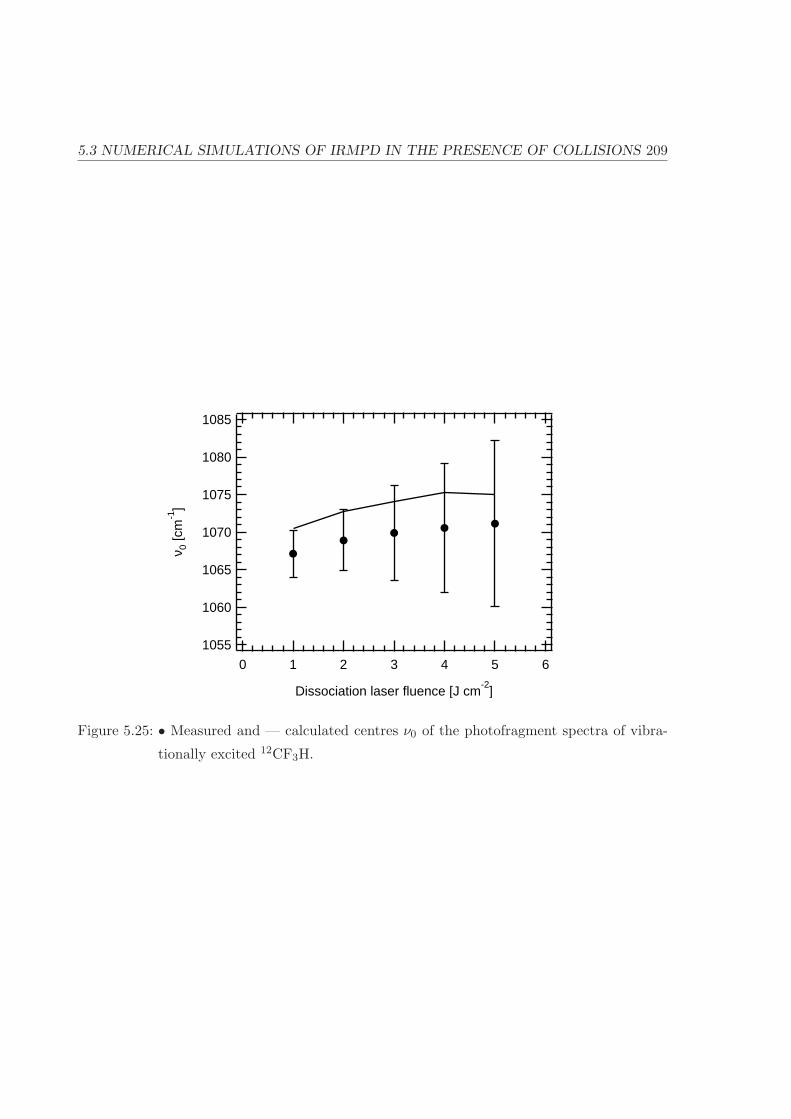
5.3 NUMERICAL SIMULATIONS OF IRMPD IN THE PRESENCE OF COLLISIONS 209
1085
1080
1075
1070
1065
1060
1055
ν 0 [c
m-1
]
6543210
Dissociation laser fluence [J cm-2
]
Figure 5.25: • Measured and — calculated centres ν0 of the photofragment spectra of vibra-
tionally excited 12CF3H.

210 CHAPTER 5. NUMERICAL SIMULATIONS
(II) Simulation of the dissociation selectivity
We now consider the data presented in sections 4.3.3. We measured the ratio of dissoci-
ation probabilities for the two isotopic species pre-excited via the 31 band for different
dissociation laser wavelengths and fluences. This ratio, Sd = 13D/ 12D, where xD is
the dissociation probability of the xCF3H molecule, is called the dissociation selectivity.
We have also measured Sd for one particular dissociation laser wavelength for molecules
pre-excited via the 21 band.
Figure 5.26 shows the measured and simulated dissociation selectivities for a disso-
ciation laser frequency of 1047 cm−1, for molecules pre-excited via the 21 (left graph)
and the 31 (right graph) bands.
60
50
40
30
20
10
0
Sd
1086420
Dissociation laser fluence [J cm-2
]
(a) Pre-excitation via the 21 band.
3.0
2.5
2.0
1.5
1.0
0.5
0.0
Sd
1086420
Dissociation laser fluence [J cm-2
]
(b) Pre-excitation via the 31 band.
Figure 5.26: — Simulated and • measured dissociation selectivities for a sample at 0.4 mbar.
The graphs show that the simulations for pre-excitation via the 31 band describe the
experimental data very well taking into account the complexity of the problem. For
molecules pre-excited via the 21 band, this is however not true: there is only a quali-
tative correspondence, but quantitatively the values differ considerably (figure 5.26-a).
Computed values for Sd lie too high, which means that either the dissociation yield
of 13CF3H is overestimated or the dissociation yield of 12CF3H is underestimated. We
believe that the latter is true because 12CF3H molecules at vCH = 2 are off-resonant
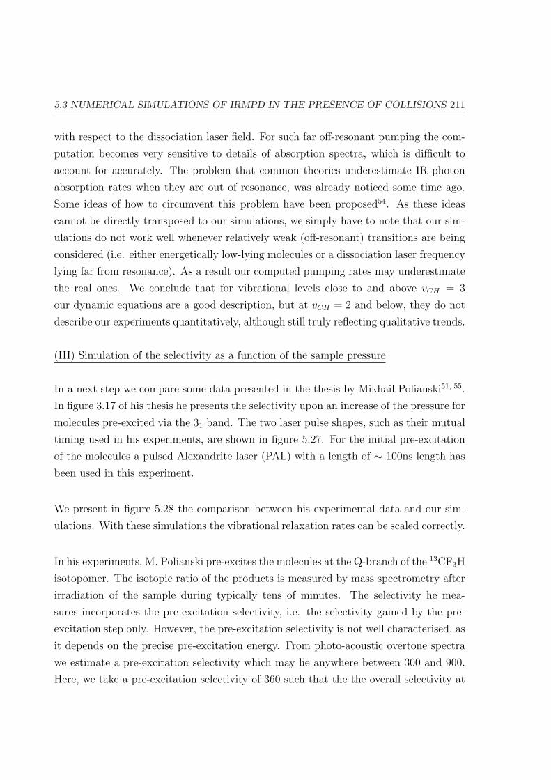
5.3 NUMERICAL SIMULATIONS OF IRMPD IN THE PRESENCE OF COLLISIONS 211
with respect to the dissociation laser field. For such far off-resonant pumping the com-
putation becomes very sensitive to details of absorption spectra, which is difficult to
account for accurately. The problem that common theories underestimate IR photon
absorption rates when they are out of resonance, was already noticed some time ago.
Some ideas of how to circumvent this problem have been proposed54. As these ideas
cannot be directly transposed to our simulations, we simply have to note that our sim-
ulations do not work well whenever relatively weak (off-resonant) transitions are being
considered (i.e. either energetically low-lying molecules or a dissociation laser frequency
lying far from resonance). As a result our computed pumping rates may underestimate
the real ones. We conclude that for vibrational levels close to and above vCH = 3
our dynamic equations are a good description, but at vCH = 2 and below, they do not
describe our experiments quantitatively, although still truly reflecting qualitative trends.
(III) Simulation of the selectivity as a function of the sample pressure
In a next step we compare some data presented in the thesis by Mikhail Polianski51, 55.
In figure 3.17 of his thesis he presents the selectivity upon an increase of the pressure for
molecules pre-excited via the 31 band. The two laser pulse shapes, such as their mutual
timing used in his experiments, are shown in figure 5.27. For the initial pre-excitation
of the molecules a pulsed Alexandrite laser (PAL) with a length of ∼ 100ns length has
been used in this experiment.
We present in figure 5.28 the comparison between his experimental data and our sim-
ulations. With these simulations the vibrational relaxation rates can be scaled correctly.
In his experiments, M. Polianski pre-excites the molecules at the Q-branch of the 13CF3H
isotopomer. The isotopic ratio of the products is measured by mass spectrometry after
irradiation of the sample during typically tens of minutes. The selectivity he mea-
sures incorporates the pre-excitation selectivity, i.e. the selectivity gained by the pre-
excitation step only. However, the pre-excitation selectivity is not well characterised, as
it depends on the precise pre-excitation energy. From photo-acoustic overtone spectra
we estimate a pre-excitation selectivity which may lie anywhere between 300 and 900.
Here, we take a pre-excitation selectivity of 360 such that the the overall selectivity at
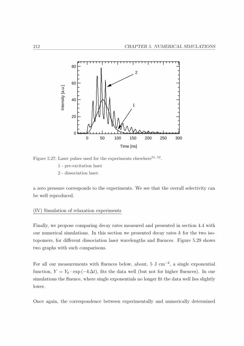
212 CHAPTER 5. NUMERICAL SIMULATIONS
80
60
40
20
0
Inte
nsity
[a.u
.]
300250200150100500
Time [ns]
1
2
Figure 5.27: Laser pulses used for the experiments elsewhere51, 52.
1 - pre-excitation laser
2 - dissociation laser.
a zero pressure corresponds to the experiments. We see that the overall selectivity can
be well reproduced.
(IV) Simulation of relaxation experiments
Finally, we propose comparing decay rates measured and presented in section 4.4 with
our numerical simulations. In this section we presented decay rates k for the two iso-
topomers, for different dissociation laser wavelengths and fluences. Figure 5.29 shows
two graphs with such comparisons.
For all our measurements with fluences below, about, 5 J cm−2, a single exponential
function, Y = Y0 · exp (−k∆t), fits the data well (but not for higher fluences). In our
simulations the fluence, where single exponentials no longer fit the data well lies slightly
lower.
Once again, the correspondence between experimentally and numerically determined
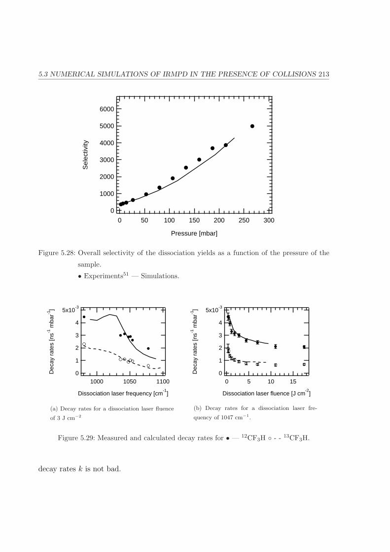
5.3 NUMERICAL SIMULATIONS OF IRMPD IN THE PRESENCE OF COLLISIONS 213
6000
5000
4000
3000
2000
1000
0
Sel
ectiv
ity
300250200150100500
Pressure [mbar]
Figure 5.28: Overall selectivity of the dissociation yields as a function of the pressure of the
sample.
• Experiments51 — Simulations.
5x10⁻³
4
3
2
1
0Dec
ay r
ates
[ns-1
mba
r-1]
110010501000
Dissociation laser frequency [cm-1
]
(a) Decay rates for a dissociation laser fluence
of 3 J cm−2
5x10⁻³
4
3
2
1
0Dec
ay r
ates
[ns-1
mba
r-1]
151050
Dissociation laser fluence [J cm-2
]
(b) Decay rates for a dissociation laser fre-
quency of 1047 cm−1.
Figure 5.29: Measured and calculated decay rates for • — 12CF3H - - 13CF3H.
decay rates k is not bad.
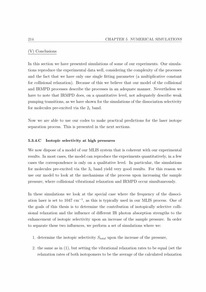
214 CHAPTER 5. NUMERICAL SIMULATIONS
(V) Conclusions
In this section we have presented simulations of some of our experiments. Our simula-
tions reproduce the experimental data well, considering the complexity of the processes
and the fact that we have only one single fitting parameter (a multiplicative constant
for collisional relaxation). Because of this we believe that our model of the collisional
and IRMPD processes describe the processes in an adequate manner. Nevertheless we
have to note that IRMPD does, on a quantitative level, not adequately describe weak
pumping transitions, as we have shown for the simulations of the dissociation selectivity
for molecules pre-excited via the 21 band.
Now we are able to use our codes to make practical predictions for the laser isotope
separation process. This is presented in the next sections.
5.3.4.C Isotopic selectivity at high pressures
We now dispose of a model of our MLIS system that is coherent with our experimental
results. In most cases, the model can reproduce the experiments quantitatively, in a few
cases the correspondence is only on a qualitative level. In particular, the simulations
for molecules pre-excited via the 31 band yield very good results. For this reason we
use our model to look at the mechanisms of the process upon increasing the sample
pressure, where collisional vibrational relaxation and IRMPD occur simultaneously.
In these simulations we look at the special case where the frequency of the dissoci-
ation laser is set to 1047 cm−1, as this is typically used in our MLIS process. One of
the goals of this thesis is to determine the contribution of isotopically selective colli-
sional relaxation and the influence of different IR photon absorption strengths to the
enhancement of isotopic selectivity upon an increase of the sample pressure. In order
to separate these two influences, we perform a set of simulations where we:
1. determine the isotopic selectivity Stotal upon the increase of the pressure,
2. the same as in (1), but setting the vibrational relaxation rates to be equal (set the
relaxation rates of both isotopomers to be the average of the calculated relaxation
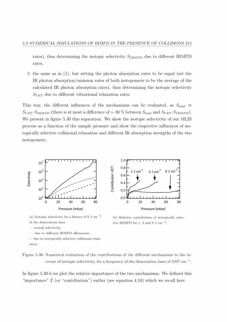
5.3 NUMERICAL SIMULATIONS OF IRMPD IN THE PRESENCE OF COLLISIONS 215
rates), thus determining the isotopic selectivity SIRMPD due to different IRMPD
rates,
3. the same as in (1), but setting the photon absorption rates to be equal (set the
IR photon absorption/emission rates of both isotopomers to be the average of the
calculated IR photon absorption rates), thus determining the isotopic selectivity
SV ET due to different vibrational relaxation rates.
This way, the different influences of the mechanisms can be evaluated, as Stotal ≈SV ET ·SIRMPD (there is at most a difference of∼ 30 % between Stotal and SV ET ·SIRMPD).
We present in figure 5.30 this separation. We show the isotopic selectivity of our MLIS
process as a function of the sample pressure and show the respective influences of iso-
topically selective collisional relaxation and different IR absorption strengths of the two
isotopomers.
100
101
102
103
104
Sel
ectiv
ity
806040200
Pressure [mbar]
(a) Isotopic selectivity for a fluence of 9 J cm−2
of the dissociation laser.
— overall selectivity.
· · · due to different IRMPD efficiencies.
- - due to isotopically selective collisional relax-
ation.
1.0
0.8
0.6
0.4
0.2
0.0
Con
trib
utio
n V
ET
806040200
Pressure [mbar]
3 J cm-2 9 J cm
-21 J cm
-2
(b) Relative contribution of isotopically selec-
tive IRMPD for 1, 3 and 9 J cm−2.
Figure 5.30: Numerical evaluation of the contributions of the different mechanisms to the in-
crease of isotopic selectivity, for a frequency of the dissociation laser of 1047 cm−1.
In figure 5.30-b we plot the relative importance of the two mechanisms. We defined this
“importance” I (or “contribution”) earlier (see equation 4.10) which we recall here

216 CHAPTER 5. NUMERICAL SIMULATIONS
Ix :=Sx − 1∑
i
(Si − 1), (5.59)
where S is the selectivity, x = due to isotopically selective vibrational relaxation / due
to IRMPD and i sums over the two possible x. We see in figure 5.30-b that for low
pressures all selectivity S is due to different IRMPD rates (which is expected, because
there is no collisional relaxation taking place). As the pressure is increased, the relative
influence of collisional relaxation increases. For 3 J cm−2 both effects are equally as
important at ∼50 mbar, for higher fluences the influence of different IR absorption
strengths stays predominant.
5.3.4.D IRMPD properties of vibrationally pre-excited CF3H
In a previous section we have shown that our model describes the experiments in a
satisfying manner. We are interested in having a general feeling of the dependency
of the dissociation yield for different pre-excitation energies as a function of different
parameters such as the pressure and the CO2 dissociation laser fluence and frequency.
Figure 5.31 shows an example of a calculated dissociation probability as a function
of the pre-excitation energy, for a given fluence and frequency of the dissociation laser
and for a given sample pressure. The timing of the lasers is kept fixed (zero time-delay
between pre-excitation (YAG) and CO2 dissociation lasers).
We show in figure 5.32 dissociation probabilities for a set of different parameters.
5.3.4.E Predictions for MLIS
We can employ this proven model to make some predictions useful for molecular laser
isotope separation (MLIS). For this, we depart from the MLIS scheme presented else-
where51, 52 where the pre-excitation laser and the dissociation laser are temporally over-
lapped (see figure 5.27 on page 212). Experimentally, this configuration has been deter-
mined to be at least close to the ideal configuration. Here, we vary numerically different
parameters in order to determine their relative influences.

5.3 NUMERICAL SIMULATIONS OF IRMPD IN THE PRESENCE OF COLLISIONS 217
1.0
0.8
0.6
0.4
0.2
0.0
Dis
soci
atio
n pr
obab
ility
12000800040000
Pre-excitation Energy [cm-1
]
Figure 5.31: Simulated dissociation probability for — 12CF3H and - - 13CF3H molecules, for
a dissociation laser frequency ν = 1047 cm−1, a dissociation laser fluence Φ =
3 J cm−2 and a sample pressure p = 1 mbar.
In figure 5.33 we show the dissociation selectivity and yield as a function of the pressure
for pre-excitation via the second and the third overtone of the CH stretching bending
vibration‡.
It can be seen that for this MLIS scheme (overlapped pulses and high pressure) that
the second overtone of the CH stretching bending vibration is better suited than the
third overtone as far as the selectivity of the dissociation step is concerned. For the
same pressure, the dissociation probabilities are the same for the 13CF3H species, but
the dissociation selectivity is higher for the lower pre-excitation level. Figure 5.34 shows
analogous data for different CO2 laser fluences.
The figures demonstrate the problem of choosing the correct dissociation laser fluence:
for low fluences, the dissociation selectivity increases which is, however, accompanied
by a simultaneous drop of the absolute dissociation yield. From the data shown here it
‡Simulations for pre-excitation via the first overtone are left away, as we have shown that those results are
only qualitatively correct, not quantitatively.
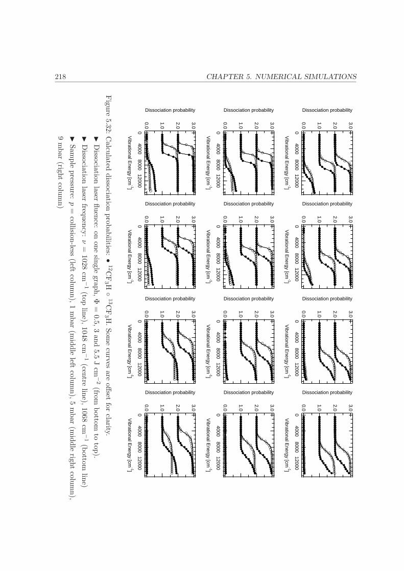
218 CHAPTER 5. NUMERICAL SIMULATIONS
3.0
2.0
1.0
0.0
Dissociation probability
120008000
40000
Vibrational E
nergy [cm-1]
3.0
2.0
1.0
0.0
Dissociation probability
120008000
40000
Vibrational E
nergy [cm-1]
3.0
2.0
1.0
0.0
Dissociation probability
120008000
40000
Vibrational E
nergy [cm-1]
3.0
2.0
1.0
0.0
Dissociation probability
120008000
40000
Vibrational E
nergy [cm-1]
3.0
2.0
1.0
0.0
Dissociation probability
120008000
40000
Vibrational E
nergy [cm-1]
3.0
2.0
1.0
0.0
Dissociation probability
120008000
40000
Vibrational E
nergy [cm-1]
3.0
2.0
1.0
0.0
Dissociation probability
120008000
40000
Vibrational E
nergy [cm-1]
3.0
2.0
1.0
0.0
Dissociation probability
120008000
40000
Vibrational E
nergy [cm-1]
3.0
2.0
1.0
0.0
Dissociation probability
120008000
40000
Vibrational E
nergy [cm-1]
3.0
2.0
1.0
0.0
Dissociation probability
120008000
40000
Vibrational E
nergy [cm-1]
3.0
2.0
1.0
0.0
Dissociation probability
120008000
40000
Vibrational E
nergy [cm-1]
3.0
2.0
1.0
0.0
Dissociation probability12000
80004000
0
Vibrational E
nergy [cm-1]
Figure
5.32:C
alculateddissociation
probabilities:•12C
F3 H
13C
F3 H
.Som
ecurves
areoffset
forclarity.
ID
issociationlaser
fluence:on
onesingle
graph,Φ
=0.5,
3and
5.5J
cm−
2(from
bottomto
top).
ID
issociationlaser
frequency:ν
=1028
cm−
1(top
line),1048
cm−
1(centre
line),1068
cm−
1(bottom
line)
ISam
plepressure:
p=
collision-less(left
column),1
mbar
(middle
leftcolum
n),5m
bar(m
iddleright
column),
9m
bar(right
column)
5.3 NUMERICAL SIMULATIONS OF IRMPD IN THE PRESENCE OF COLLISIONS 219
8
6
4
2
0
SIR
MP
D
200150100500
pressure [mbar]
(a) Selectivity.
1.0
0.8
0.6
0.4
0.2
0.0
D (
13C
F3H
)
200150100500
pressure [mbar]
(b) Dissociation probability of 13CF3H.
Figure 5.33: Dissociation selectivity and yield for pre-excitation via the - - 31 and the — 41
bands, for a dissociation laser frequency of 1044 cm−1 and fluence of 3 J cm−2.
20
15
10
5
0
SIR
MP
D
200150100500
pressure [mbar]
(a) Selectivity.
1.0
0.8
0.6
0.4
0.2
0.0
D (
13C
F3H
)
200150100500
pressure [mbar]
(b) Dissociation probability of 13CF3H.
Figure 5.34: Dissociation selectivity and yield for a dissociation laser fluence of · · · 1, - - 3 and
— 5 J cm−2, for pre-excitation via the 31 band and a dissociation laser frequency
of 1044 cm−1.
can be seen that a fluence of 3 J cm−2 is a good compromise if one desires a relatively
high dissociation probability. Finally, figure 5.35 shows analogous data for different CO2
laser frequencies.
From this figure it can be seen, that by changing the dissociation laser fluence from

220 CHAPTER 5. NUMERICAL SIMULATIONS
10
8
6
4
2
0
SIR
MP
D
200150100500
pressure [mbar]
(a) Selectivity.
1.0
0.8
0.6
0.4
0.2
0.0
D (
13C
F3H
)
200150100500
pressure [mbar]
(b) Dissociation probability of 13CF3H.
Figure 5.35: Dissociation selectivity and yield for a dissociation laser frequency of · · · 1039,
- - 1044 and — 1049 cm−1, for pre-excitation via the 31 band and a dissociation
laser fluence of 3 J cm−2.
1044 cm−1 down to 1039 cm−1, some selectivity (a factor of 2-3 for typical pressures
of 50-100 mbar) can be gained without any significant change of the productivity. For
this reason, we propose that for a potential industrial application the dissociation laser
frequency should be chosen as far to the red as possible within the 9P emission band
of the CO2 laser (∼1039 cm−1). For the next emission band of the dissociation laser
(∼970-980 cm−1), the absolute yields however are to low to be industrially interesting.
5.3.5 Summary and discussion
Section 5.3 was devoted to simulations of the IRMPD process of pre-excited CF3H
molecules in the presence of collisions. In section 5.3.1 we introduced the basic ideas
of our simulations, in section 5.3.2 we developed the master equation which has to be
solved numerically and in section 5.3.3 we explained how to evaluate physically reason-
able values for the different rate coefficients needed in our master equation. Basically,
for the interaction of a molecule with the field of the dissociation laser we applied a
statistical theory presented in section 2.2, for vibrational relaxation we used the numer-
ical results obtained in section 5.2 and for unimolecular dissociation we applied RRKM
theory. The pumping rates due to the dissociation laser have been generalised by in-
troducing a dependency on the dissociation laser frequency, the excitation level of the
5.3 NUMERICAL SIMULATIONS OF IRMPD IN THE PRESENCE OF COLLISIONS 221
molecule and its isotopic species.
In section 5.3.4 we presented our results. After a first general introduction, we pre-
sented a comparison between the numerical simulations and experiments:
• We simulated photofragment spectra which have been measured experimentally
(see section 4.3). We noticed the necessity of introducing absorption of IR photons
by increasing the number of quanta in the ν6 vibration by two. In this case, there
is an excellent agreement between experiments and numerical simulations.
• Simulations of dissociation selectivities (experiments presented in sections 4.3.3)
showed an excellent agreement for molecules pre-excited via the 31 band. For
molecules pre-excited via the 21 band the agreement is only on a qualitative level.
We explained that the discrepancy is because in this case 12CF3H molecules are
very much out of resonance with the dissociation laser field, and in such cases the
absorption rates are underestimated.
• We calculated the dissociation selectivity of pre-excited CF3H molecules as a func-
tion of the sample pressure in order to scale the vibrational relaxation rates.
• Also simulated decay rates fit very well with experimental data. The only dis-
crepancy is that single exponentials do not fit absolutely well to simulated decay
curves as opposed to experimental data. However, using such exponentials for the
fit, the decay rates k correspond astonishingly good to the experimental data.
In these simulations, we worked with one single fitting parameter, a multiplicative con-
stant for the vibrational relaxation rates. This scaling factor has been determined by
fitting our results to different types of experiments.
With this set of simulations we are convinced that our model is a good and neces-
sary model and that it describes reality in a satisfactory manner. With this, we were
able to perform simulations in which we can observe the mechanisms of the OP-IRMPD
process, and we can also perform simulations that have not been or cannot be performed
experimentally.
222 CHAPTER 5. NUMERICAL SIMULATIONS
Two sets of numerical experiments have been performed. First, in section 5.3.4.C we
have shown how we determined the following:
At higher working pressures, isotopically selective collisional relaxation and different
IR photon absorption rates both contribute to the enhancement of isotopic selectivity of
the dissociation yield. For typical conditions we propose, the main contribution comes
from different IRMPD rates.
We performed simulations where we evaluate the dissociation yield as a function of
different experimental conditions such as the fluence and the frequency of the disso-
ciation laser and the pressure of the sample. We have found that, in general, for an
optimal dissociation selectivity in a real MLIS process, pre-excitation has to be done up
to the first or the second overtone of the C-H stretch vibration, depending on different
experimental parameters.
We have given some general features of the OP-IRMPD process. For a practical appli-
cation at higher pressures and with overlapped pre-excitation and dissociation lasers52
we propose to use a dissociation laser frequency on the red side of the 9P emission band
of the CO2 laser.
Bibliography
[1] Aleksei Stuchebrukhov, Stanislav Ionov, and Vladilen Letokhov. IR Spectra of
Highly Vibrationally Excited Large Polyatomic Molecules and Intramolecular Re-
laxation . J. Phys. Chem., 93:5357–5365, 1989.
[2] A. L. Malinovsky, I. Yu. Petrova, E. A. Ryabov, A. A. Makarov, and V. S. Letokhov.
Transition Spectra in the Vibrational Quasicontinuum of Polyatomic Molecules:
Raman Spectra of Highly Excited SF6 Molecules . J. Phys. Chem. A, 102:9353–
9359, 1998.
[3] V. N. Lokhman, A. N. Petin, E. A. Ryabov, and V. S. Letokhov. Transition Spectra
in the Vibrational Quasicontinuum of Polyatomic Molecules: IR Multiple-Photon

BIBLIOGRAPHY 223
Absorption in SF6. 1. Experimental Studies . J. Phys. Chem. A, 103:11293–11298,
1999.
[4] V. N. Lokhman, A. A. Makarov, I. Yu. Petrova, E. A. Ryabov, and V. S. Letokhov.
Transition Spectra in the Vibrational Quasicontinuum of Polyatomic Molecules:
IR Multiple-Photon Absorption in SF6. 1. Theoretical Simulation and Comparison
with Experiment . J. Phys. Chem. A, 103:11299–11309, 1999.
[5] A. A. Kosterev, A. A. Makarov, A. L. Malinovsky, I. Yu. Petrova, E. A. Ryabov,
and V. S. Lethokov. Transition Spectra in the Vibrational Quasicontinuum of
Polyatomic Molecules: Raman Spectra of Highly Excited UF6 Molecules . J. Phys.
Chem. A, 104:10259–10264, 2000.
[6] S. Califano. Vibrational States. John Wiley and Sons, 1976.
[7] Philip R. Bunker and Per Jensen. Molecular Symmetry and Spectroscopy. Ottawa
: NRC Research Press, 1998.
[8] Gunter Klatt, Andrew Willetts, Nicholas C. Handy, Riccardo Tarroni, and Paolo
Palmieri. An Improved Anharmonic Potential for CHF3 . J. Molec. Spectrosc.,
176:64–74, 1996.
[9] O. V. Boyarkin, M. Kowalczyk, and T. R. Rizzo. Collisionally Enhanced Isotopic
Selectivity in Multiphoton Dissociation of vibrationally excited CF3H . J. Chem.
Phys., 118(1):93–103, 2003.
[10] N. J. Fyke, P. Lockett, J. K. Thompson, and P. M. Wilt. The Infrared Spectra of
HCF3 and DCF3 . J. Molec. Spectrosc., 58:87–101, 1975.
[11] G. Graner and G. Guelachvili. Fluoroform: the Polyad at 8-9 µm . J. Molec.
Spectrosc., 107:215–228, 1984.
[12] A. Amrein, M. Quack, and U. Schmitt. High-Resolution Interferometric Fourier-
Transform Infrared- Absorption Spectroscopy in Supersonic Free Jet Expansions -
Carbon-Monoxide, Nitric-Oxide, Methane, Ethyne, Propyne, and Trifluoromethane
. J. Phys. Chem., 92(19):5455–5466, 1988.
[13] J. P. Champion and G. Graner. Fluoroform - A new analysis of the polyad at 8-9
µm . Molec. Phys., 58(3):475–484, 1986.

224 CHAPTER 5. NUMERICAL SIMULATIONS
[14] Andreas Amrein, Martin Quack, and Ulrich Schmitt. High resolution interfero-
metric Fourier transform infrared absorption spectroscopy in a supersonic free jet
expansion - The interacting states ν2, ν5 and ν3 + ν6 of trifluoromethane . Molec.
Phys., 60(1):237–248, 1987.
[15] Gerhard Herzberg. Molecular Spectra and Molecular Structure. II. Infrared and
Raman Spectra of Polyatomic Molecules. Krieger Publishing Company: Malabar,
Florida, 1991.
[16] Alexander Makarov (ISAN Troitsk Russia). Private communication .
[17] V. T. Platonenko and N. A. Sukhareva. On vibrational energy exchange between
strongly excited polyatomic molecules . Sov. Phys. JETP, 51(6):1065–1071, 1980.
[18] V. T. Platonenko and N. A. Sukhareva. Vibrational relaxation of strongly excited
polyatomic molecules . Sov. Phys. JETP, 54(3):454–459, 1981.
[19] V. M. Akulin. Singularities of collisional vibrational relaxation processes in strongly
excited spectrally complex polyatomic molecules . Sov. Phys. JETP, 57(4):774–780,
1983.
[20] Bruce H. Mahan. Resonant Transfer of Vibrational Energy in Molecular Collisions
. J. Chem. Phys., 46(1):98–101, 1967.
[21] R. D. Sharma and C. A. Brau. Near-Resonant vibrational energy transfer in
N2-CO2 Mixtures . Phys. Rev. Lett., 19(22):1273–1275, 1967.
[22] R. D. Sharma and C. A. Brau. Energy Transfer in Near-Resonant Molecular
Collisions due to Long-Range Forces with Application to Transfer of Vibrational
Energy from ν3 Mode of CO2 to N2 . J. Chem. Phys., 50(2):924–930, 1969.
[23] R. D. Sharma. Vibration-to-Vibration energy transfer in CO-CO collisions . Chem.
Phys. Lett., 30(2):261–266, 1975.
[24] Beatriz M. Toselli and John R. Barker. Isotope effects in the vibrational deacti-
vation of large molecules . J. Chem. Phys., 97(3):1809–1817, 1992.
[25] M. Quack and G. Seyfang. Frequency-dependent non-linear intensity dependence
in the IR Photochemistry of CF3I . Chem. Phys. Lett., 93(5):442–447, 1982.
BIBLIOGRAPHY 225
[26] P. Dietrich, M. Quack, and G. Seyfang. Quantitative Infrared Photochemistry
with CO2 laser of different temporal shape: dissociation of CF3I with nanosecond
pulses . Infrared Phys., 29(2-4):517–523, 1989.
[27] Martin Quack. Master Equations for Photochemistry with Intense Infrared Light
. Ber. Bunsenges. Phys. Chem., 83:757–775, 1979.
[28] M. L. Azcarate and E. J. Quel. Isotopic Selectivity and Collisional Deactivation in
the Infrared Multiple-Photon Dissociation of CDCl3 in Equimolar CDCl3/CHCl3
Mixtures . J. Phys. Chem., 93:697–702, 1989.
[29] K. A. Holbrook, M. J. Pilling, and S. H. Robertson. Unimolecular Reactions,
chapter Kinetic Isotope Effects in Unimolecular Reactions. Wiley: Chichester,
1996.
[30] M. Quack and J. Troe. Specific rate constants of unimolecular processes. 2. Adia-
batic Channel model . Ber. Bunsenges. Phys. Chem., 78(3):240–252, 1974.
[31] Oscar Knefler Rice and Herman C. Ramsperger. Theories of unimolecular gas
reactions at low Pressures . J. Am. Chem. Soc., 49(7):1617–1629, 1927.
[32] Oscar Knefler Rice. The Quantum Theory of Quasi-Unimolecular Gas Reactions
. Proc. Natl. Acad. Sci. U.S.A., 14(2):113–118, 1928.
[33] L. S. Kassel. Studies in Homogeneous Gas Reactions. II. Introduction of Quantum
Theory . J. Phys. Chem., 32(7):1065–1079, 1928.
[34] R. A. Marcus. Lifetimes of Active Molecules. I. . J. Chem. Phys., 20(3):352–354,
1952.
[35] R. A. Marcus. Lifetimes of Active Molecules. II. . J. Chem. Phys., 20(3):355–359,
1952.
[36] R. A. Marcus. Unimolecular Dissociations and Free Radical Recombination Reac-
tions . J. Chem. Phys., 20(3):359–364, 1952.
[37] R. A. Marcus. Recombination of Methyl Radicals and Atomic Cracking of Ethyl
Radicals . J. Chem. Phys., 20(3):364–368, 1952.

226 CHAPTER 5. NUMERICAL SIMULATIONS
[38] Dong Nam Shin, Yong Sim Yoo, Chul Woong Park, Jae Won Hahn, and Kihyung
Song. Kinetic study for the unimolecular dissociation of CF3H: RRKM and PST
calculations on an ab initio potential energy surface . Chem. Phys. Lett., 258:613–
619, 1996.
[39] S. W. Benson. Thermochemical kinetics. Wiley, New York, 1976.
[40] E. Tschuikow-Roux and J. E. Marte. Thermal Decomposition of Fluoroform in a
Single-Pulse Shock Tube. I . J. Chem. Phys., 42(6):2049–2056, 1965.
[41] E. Tschuikow-Roux. Thermal Decomposition of Fluoroform in a Single-Pulse Shock
Tube. II. Pressure Dependence of the Rate . J. Chem. Phys., 42(10):3639–3642,
1965.
[42] A. P. Modica and J. E. LaGraff. Mass-Spectrometer and UV Absorption Study
of CHF3 Decomposition behind Shock Waves . J. Chem. Phys., 44(9):3375–3379,
1966.
[43] K. P. Schug, H. Gg. Wagner, and F. Zabel. Gas Phase α, α Elimination of Hydrogen
Halides from Halomethanes. I. Thermal Decomposition of Chlorodifluoromethane,
Trifluoromethane, and Trichloromethane Behind Shock Waves . Ber. Bunsenges.
Phys. Chem., 83:167–175, 1979.
[44] Yoshiaki Hidaka, Takuji Nakamura, and Hiroyuki Kawano. High temperature
pyrolysis of CF3H in shock waves . Chem. Phys. Lett., 187(1,2):40–44, 1991.
[45] Georg Seyfang (ETH Zurich Switzerland). Private communication .
[46] Lars Melander. Isotope Effects on Reaction Rates. Ronald Press Company: New
York, 1960.
[47] Keith J. Laidler. Chemical Kinetics, chapter Isotope Effects. Harper & Row, New
York, 1987.
[48] Martin Quack. Theory of unimolecular reactions induced by monochromatic in-
frared radiation . J. Chem. Phys., 69(3):1282–1307, 1978.
[49] Martin Quack. Master Equations for Photochemistry with Intense Infrared Light
(IV). A Unified Treatment of Case B and Case C Including Nonlinear Effects . Ber.
Bunsenges. Phys. Chem., 85:318–330, 1981.

BIBLIOGRAPHY 227
[50] John Charles Butcher. The numerical analysis of ordinary differential equations :
Runge-Kutta and general linear methods. Chichester a.o. : Wiley, 1987.
[51] Mikhail N. Polianski. Overtone pre-excitation - Infrared Multiple Photon Dissoci-
ation Under Collisional Conditions. New Potential for Laser Isotope Separation .
PhD thesis, Ecole polytechnique federale de Lausanne, Switzerland, 2004.
[52] M. Polianski, O. V. Boyarkin, and T.R. Rizzo. Collisionally-assisted, highly-
selective laser isotope separation of carbon-13 . J. Chem. Phys., 121(23):11771–
11779, 2004.
[53] A. Ceausu-Velcescu, H. Burger, and G. Graner. High-resolution infrared spectra
of HCF3 in the ν6 (500 cm−1) and 2ν6 (1000 cm−1) regions: rovibrational analysis
and accurate determination of the ground state constants C0 and D0K . J. Molec.
Spectrosc., 220:298–305, 2003.
[54] V. S. Letokhov and A. A. Makarov. “Leakage” effect as an Exciting Mechanism
of High Vibrational Levels of Polyatomic Molecules by a Strong Quasi-Resonant
Laser IR Field . Optics Comm., 17(3):250–253, 1976.
[55] M. Polianski, O. V. Boyarkin, and T. R. Rizzo. to be published . 2005.

228 CHAPTER 5. NUMERICAL SIMULATIONS
Chapter 6
Conclusions and Outlook
The goal of this thesis was to explain the increase of isotopic selectivity in our OP-
IRMPD molecular laser isotope separation process upon increasing the sample pressure
or the time-delay between the two lasers. We have performed a set of experiments and
numerical simulations and we are able to give a coherent picture of this enhancement.
Furthermore, we have directly observed isotopically selective collisional vibrational re-
laxation of highly excited medium-sized polyatomic molecules which is, to the best
of our knowledge, the first in its kind. We have proposed a model including both
short-distance and long-distance interactions between two CF3H molecules which is in
a satisfying agreement with our experimental findings.
6.1 Isotopically selective collisional vibrational relaxation
We have performed experiments where we measure the total dissociation yield using
the OP-IRMPD process as a function of the time-delay between the pre-excitation and
dissociation laser. By letting either excited 12CF3H or 13CF3H relax on ground state12CF3H or 13CF3H we were able to measure relative relaxation rates of self and cross-
relaxation (13CF3H on 12CF3H and vice versa). The finding is that in general the
molecules relax roughly 1.5-2.5 as fast on 13CF3H than on 12CF3H (see figure 4.26).
Table 6.1 summarises the final result.
There is a small uncertainty as to the absolute relaxation rates, because our detection
via IRLAPS senses molecules over an energy region which is not a priori well known.
229

230 CHAPTER 6. CONCLUSIONS AND OUTLOOK
Pre-excitation energy κ(12? − 12) : κ(12? − 13) : κ(13? − 13) : κ(13? − 12)
5950 cm−1 1.00 : 1.60 : 1.00 : 0.41
8800 cm−1 1.00 : 1.94 : 1.00 : 0.51
11,530 cm−1 1.00 : 1.90 : 1.00 : 0.57
14,000 cm−1 1.00 : 1.65 : 1.00 : 0.59
Table 6.1: Summary of relative relaxation rates of excited CF3H on ground state CF3H. κ(X?−Y ) is the relaxation rate of excited XCF3H on ground state Y CF3H.
We have proposed a numerical model for the explanation of these results. In this
model, vibrational energy transfer is mediated by (a) the repulsive part of the (short-
range) interaction potential of the two molecules and (b) the long-range dipole-dipole
interactions. Collisional relaxation due to (a) is very difficult to handle, which is why we
treat this part as an adjustable parameter. For the vibrational relaxation rate W due
to part (b) relatively precise calculations can be done based on the Fermi golden rule
W = 2π|V |2ρ/~. Here, V can be related to the IR absorption spectra of molecules in the
ground state, and ρ can be related to the overlap of the absorption spectra of molecules in
the ground state and emission spectra of the excited molecules. These emission spectra
had to be calculated, taking into account a so-called “statistical inhomogeneous broad-
ening”1 due to large intramolecular mode mixing. Our model resembles those proposed
by Mahan2 and Sharma and Brau3–5, where a similar distinction between long-range
and short-range interactions has been made. At some point these authors have to as-
sume a certain value for the cut-off distance that separates long-range and short-range
interactions, and they also have to assume a certain vibrational energy transfer proba-
bility mediated by short-range interactions. As we possess a set of measurements with
isotopically substituted molecules, we fit these parameters rather than assuming certain
values. The fitted values, ∼7.4 A for the cut-off radius, and ∼ 6.8 ·104/E the number of
collisions for the molecule to lose 1000 cm−1 in short-range interactions, are physically
reasonable, which makes our model credible. To our knowledge, this is the first time
that such calculations have been performed for highly excited polyatomics where such
extensive mixing has to be taken into account.

6.2. ENHANCEMENT OF ISOTOPIC SELECTIVITY IN OUR MLIS PROCESS 231
6.2 Enhancement of isotopic selectivity in our MLIS process
We have performed a series of experiments to determine the mechanism of the enhance-
ment of isotopic selectivity by increasing the time-delay at low pressures. Basically, two
questions have to be answered. First, is this phenomenon specific to CF3H molecules
pre-excited via the 31 band and due to some accidental resonances of this band with
others ? And secondly, if not, what mechanisms apply ?
By changing the pre-excitation energy to different rovibrational bands, we have de-
termined unambiguously that the phenomenon is not specific to the pre-excited rovi-
brational state, but general, and may hence be used for other molecules. In a set of ex-
periments we have determined the respective influence of isotopically selective collisional
relaxation and different absorption strengths of IR photons for different pre-excitation
energies and fluences of the dissociation laser. Interestingly enough, both mechanisms
contribute in general roughly 50 % to the enhancement of isotopic selectivity.
In a second step we developed numerical master equations for the description and
calculation of the OP-IRMPD process. We showed in a set of simulations, that our
experimental data is relatively well reproduced, which makes our simulations credible.
With this, we could simulate experiments at higher pressures, and we could show, that
for a fluence of 3 J cm−2 and a frequency of 1047 cm−1 of the CO2 dissociation laser
both mechanisms contribute significantly to the enhancement of isotopic selectivity, al-
though the influence of different IRMPD rates is predominant.
In view of finding an ideal parent molecule for MLIS via collisionally assisted OP-
IRMPD, different criteria must be met. There are some chemical constraints which
were not subject of this thesis. These constraints include the capacity of the dissoci-
ation product recombining with each other or with a scavenger gas to form a stable
product. From a point of view of efficiently and selectively bringing the molecules to
dissociate, we summarise the key properties that such a molecule should have:
1. Large absorption coefficient for an overtone of a certain mode. This is typically
achieved in molecules with a C-H bond which is in general very anharmonic, and
as a consequence the absorption is relatively strong.
232 CHAPTER 6. CONCLUSIONS AND OUTLOOK
2. A well resolved isotopic shift for pre-excitation.
3. A large isotopic shift for the mode that has the largest transition dipole moment
(for V-V relaxation to be as selective as possible). Ideally, the intra- and intermode
anharmonicity for this vibration should be as small as possible (in order to conserve
isotopic selectivity of VET upon excitation of the molecule).
4. A well absorbing vibration to the blue of the dissociation laser such that an efficient
discrimination between ground state molecules and excited molecules can be done
for IRMPD, and a large isotopic shift for this particular vibrational mode.
For the case that this scheme should ever be employed in an industrial laser isotope
separation plant, we propose the use of a (strong) CO2 laser line at the low frequency
end of the 9P emission band of CO2 (∼ 1039 cm−1).
Bibliography
[1] Aleksei Stuchebrukhov, Stanislav Ionov, and Vladilen Letokhov. IR Spectra of
Highly Vibrationally Excited Large Polyatomic Molecules and Intramolecular Re-
laxation . J. Phys. Chem., 93:5357–5365, 1989.
[2] Bruce H. Mahan. Resonant Transfer of Vibrational Energy in Molecular Collisions
. J. Chem. Phys., 46(1):98–101, 1967.
[3] R. D. Sharma and C. A. Brau. Near-Resonant vibrational energy transfer in N2-CO2
Mixtures . Phys. Rev. Lett., 19(22):1273–1275, 1967.
[4] R. D. Sharma and C. A. Brau. Energy Transfer in Near-Resonant Molecular Colli-
sions due to Long-Range Forces with Application to Transfer of Vibrational Energy
from ν3 Mode of CO2 to N2 . J. Chem. Phys., 50(2):924–930, 1969.
[5] R. D. Sharma. Vibration-to-Vibration energy transfer in CO-CO collisions . Chem.
Phys. Lett., 30(2):261–266, 1975.

APPENDICES


Appendix A
Development of formulae for
pumping molecules through a low
density regime (“case C”)
The formulae for the up- and down-pumping constants KJ,I for the case of essentially
uncoupled levels within an energy bin (“case C”) are given in table 2.12. Here we
first give some qualitative explanations of how the formulae have been calculated (sec-
tion A.1). Quantitative explanations can be found in section A.2.
The case C calculations are explicitly given for the initial condition that the upper
level J is not populated at t = 0 and stays sparsely populated throughout the experi-
ment. This condition is reasonably well fulfilled for IRMPD of ground state molecules.
In our case however, we populate a certain level with the pre-excitation laser (overtone
of C-H stretch vibration). If we look at the up and down-pumping rates between this
populated level (≡ level J) and a level lying ∼1,050 cm−1 (energy of CO2 laser photon)
below it (≡ level I) the situation is inverted. The upper level is initially populated and
the lower level is unpopulated. We hence have to generalise the formulae for case C or
at least adapt it to our calculations. Section A.3 treats this problem.
235

236APPENDIX A. DEVELOPMENT OF FORMULAE FOR PUMPING MOLECULES
THROUGH A LOW DENSITY REGIME (“CASE C”)
A.1 Qualitative explanations
In case C the states within both grained levels I and J are not anharmonically coupled
between each other, but there is a pairwise interaction due the IR field between mem-
bers of levels I and J (figure A.1)‡.
Figure A.1: In case C, the states in both the upper and lower bins are uncoupled amongst
each other. Coupling occurs only between members of bin I and bin J via laser
radiation.
The total evolution of population corresponds hence to the average of the population
evolutions between the individual couple of states.
For each pair of coupled states i and j (pi(t = 0) = 1 and pj(t = 0) = 0), the population
evolution is described by Rabi-oscillations. The amplitude of these oscillations is mainly
given by the off-resonance shift D = ω − (Ej − Ei) where ω is the energy of a laser
photon and Ei and Ej are the energies of the upper and the lower levels respectively.
The smaller D, the larger the amplitude of oscillations (in the limiting case of D = 0
‡Unfortunately there is a small inconsistency in the theory: on the one hand one assumes that the states
within a bin are uncoupled, but on the other hand one sums over all couples of states, therefore assuming
that the states are equally populated. This inconsistency has to be accepted if one wants to apply the master
equation calculations.

A.1. QUALITATIVE EXPLANATIONS 237
there is a complete population transfer i → j → i → j → . . .). The frequency of the
population transfer also depends, although weaker, on D. Figure A.2 demonstrates this
population transfer.
1.0
0.8
0.6
0.4
0.2
0.0
Pop
ulat
ion
of le
vel j
Time
A
C
B
Figure A.2: Rabi-oscillations for different strengths of coupling between the two states. The
curves show the population of the upper level j which is initially unpopulated.
A measure of the coupling is given by D/V where D is the off-resonance shift
between the laser field and the difference in energy of the two states and V is the
strength of the laser field.
(A) Strong coupling (D ¿ V ).
(B) Intermediate coupling (D ≈ V ).
(C) Weak coupling (D À V ).
The total population in a bin is obtained after averaging over all members of this bin:
pJ(t) =
N∑i=1
pji(t)
N, (A.1)
where N is the number of coupled pairs of states (analogously for bin I). Here small
i, j’s refer to single states in a bin, and capital I, J ’s refer to the bins themselves.
With some assumptions about how Di and Vi (strength of coupling via the laser) are
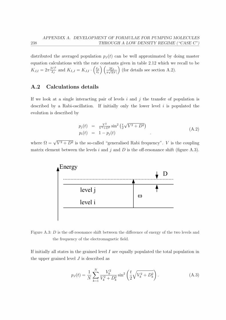
238APPENDIX A. DEVELOPMENT OF FORMULAE FOR PUMPING MOLECULES
THROUGH A LOW DENSITY REGIME (“CASE C”)
distributed the averaged population pJ(t) can be well approximated by doing master
equation calculations with the rate constants given in table 2.12 which we recall to be
KJ,I = 2π |V |2
δJand KI,J = KJ,I ·
(δJ
δI
)(2δJ
π√
3|V |
)(for details see section A.2).
A.2 Calculations details
If we look at a single interacting pair of levels i and j the transfer of population is
described by a Rabi-oscillation. If initially only the lower level i is populated the
evolution is described by
pj(t) = V 2
V 2+D2 sin2(
t2
√V 2 + D2
)
pi(t) = 1− pj(t) .(A.2)
where Ω =√
V 2 + D2 is the so-called “generalised Rabi frequency”. V is the coupling
matrix element between the levels i and j and D is the off-resonance shift (figure A.3).
Figure A.3: D is the off-resonance shift between the difference of energy of the two levels and
the frequency of the electromagnetic field.
If initially all states in the grained level I are equally populated the total population in
the upper grained level J is described as
pJ(t) =1
N
N∑
k=1
V 2k
V 2k + D2
k
sin2
(t
2
√V 2
k + D2k
). (A.3)

A.2. CALCULATIONS DETAILS 239
If there are a lot of coupled levels (N → large) the sum can be replaced by integrals
over V and D which read
pJ(t) =
∞∫−∞
dDF (D)∞∫−∞
dV G(V ) V 2
V 2+D2 sin2(
t2
√V 2 + D2
)
∞∫−∞
dDF (D)∞∫−∞
dV G(V )
, (A.4)
where, however, F and G are completely unknown.
This equation is not easy to evaluate, even if some special forms of F (D) and G(V ) are
assumed. One can however evaluate the behaviour as t → ∞ and for the special case
of square functions of F and G
F (D) =
CD −Dm ≤ D ≤ Dm
0 otherwise
G(V ) =
CV −Vm ≤ V ≤ Vm
0 otherwise
(A.5)
With this equation A.4 becomes
pJ(t) =1
DmVm
Dm∫
0
dD
Vm∫
0
dV sin2
(t
2
√V 2 + D2
)V 2
V 2 + D2. (A.6)
As t → ∞ the expression sin2(
t2
√V 2 + D2
)will be on average 1/2 and pJ is readily
evaluated
pJ(t →∞) =1
2DmVm
Dm∫
0
dD
Vm∫
0
dVV 2
V 2 + D2(A.7)
Because in case C the coupling between the states is assumed to be small, we have
Dm À Vm and the above integral becomes
pJ(t →∞) = πVm
8Dm+ 1
41− [(V 2
m + D2m) /VmDM ] arctan (Vm/Dm)
≈ πVm
8Dm.
(A.8)

240APPENDIX A. DEVELOPMENT OF FORMULAE FOR PUMPING MOLECULES
THROUGH A LOW DENSITY REGIME (“CASE C”)
Also, if equation A.4 is evaluated for D−1m ¿ t ¿ V −1
m , which is the most interesting
region, one gets
pJ(t) ≈ V 2m
4Dm
t. (A.9)
By setting1 V 2m = 12|V |2 and Dm = δ/2 where |V | is the average interaction defined in
table 2.11 and δ is the average spacing between effectively coupled levels we get
pJ(t) =
π√
3|V |2δJ
t →∞6|V |2
δJt D−1
m ¿ t ¿ V −1m
. (A.10)
In our calculations we do not consider the individual coupling between states, but we
seek to describe the evolution of the population of a bin with master equations using
pumping rates. We can set pumping rates between a lower level I and an upper level J
of
KCJ,I = 2π|V |2/δJ
KCI,J =
(π√
3|V |/2δJ
)−1 · (δJ/δI) ·KJ,I ,(A.11)
where we used the approximation that 2π ≈ 6 and by setting δ = δ2J/δI . This way we
get a population evolution similar to the one described above. The initial slope and the
final relaxed distributions are the same as described in equation A.10. This is illustrated
in figure A.4. The value for KCJ,I corresponds to the up-pumping value of cases A and
B, the down-pumping rate KCI,J is the same as for case B with a correction factor of(
π√
3|V |/2δJ
)−1.
For these calculations we made a certain number of approximations and assumptions.
One of these is that G and F are square functions. If they would have been assumed
e.g. gaussians, the evolution would be slightly different. This is also shown in figure A.4.
A.3 Attempts to generalise case C calculations
All the calculations presented above hold true as long as the upper level J is initially
unpopulated and that on average the coupling V is small, so that the upper level es-
sentially remains unpopulated at all times. A generalisation of case C calculations is

A.3. ATTEMPTS TO GENERALISE CASE C CALCULATIONS 241
0.10
0.08
0.06
0.04
0.02
0.00
Pop
ulat
ion
of le
vel J
100806040200
Time
Figure A.4: Evolution of upper level J (solution to equation A.4).
- - G, F are square functions (equation A.5).
· · · G, F are gaussian functions.
— Approximative solution to the case of G, F = square functions by master
equations (pumping rates in A.11).
difficult, because in our approach to use the master equation we characterise the popu-
lation distribution by their energy and not by the state (we only store |〈Ψi |Ψ(t)〉|2 in
form of pi(t) (i = 0, 1, 2, . . .) and not |Ψ(t)〉 itself, where |Ψi〉 is the state associated
with bin i, |Ψ(t)〉 is the state of the molecule). This is not sufficient if we want to
generalise these calculations.
We decide to take a pragmatic approach to this problem: when calculating the pumping-
rates, we first determine for each pair of states the one which is more populated. If the
lower state is more populated, then the formulae developed by Quack will be applied,
in the inverse situation, the formulae will be correctly inverted. This may lead to some
problems in regions where molecules in the ground state heated up by collisions and/or
IR photons absorption “meet” molecules pre-excited having lost energy due to collisions
and/or stimulated emission. However, it turns out, that the influence is marginal.

242APPENDIX A. DEVELOPMENT OF FORMULAE FOR PUMPING MOLECULES
THROUGH A LOW DENSITY REGIME (“CASE C”)
Bibliography
[1] Martin Quack. Master Equations for Photochemistry with Intense Infrared Light
(IV). A Unified Treatment of Case B and Case C Including Nonlinear Effects . Ber.
Bunsenges. Phys. Chem., 85:318–330, 1981.

Appendix B
Collisional quenching of LIF
At the pressures used in our experiments, CF2 fragments in an excited electronic state
may not only spontaneously emit a photon (LIF), but can undergo non-radiative colli-
sional deactivation. As long as we are performing experiments at a constant pressure,
this correction is simply a scaling factor having no influence on our results, since we
are only interested in relative values. However, in the experiments where we measure
pressure dependencies, the LIF signal has to be corrected for the quenching.
To determine a correction factor we measure the decrease of the LIF signal as a function
of time for different pressures. This decrease is characterised by a relaxation rate Kp
which can be expressed as
Kp =1
τ0
+ q · p, (B.1)
where τ0 is the radiative lifetime of an excited state, p is the pressure of the quenching
gas and q is the quenching constant. q is measured by fitting an exponent to the tail
of the LIF signal (at the beginning some scattered light contributes to the LIF signal).
Figure B.1 shows a sample LIF signal and the region fitted.
The radiative life-time has been determined to be τ0 = (64± 2) ·107 ns and the quench-
ing constant q = (1.10± 0.09) · 105 (mbar s)−1 (see fig B.2). The value for τ0 compares
well with the literature1–4 which which cites values of 59, 61 ± 3, 55 and 62 ± 4 ns.
The quenching rate q of CF2 on CF3H has not been measured to our knowledge, but for
CF2HCl and for CF4 they have been determined to be 6.6 · 105 and 8.8 · 104 (mbar s)−1.
243

244 APPENDIX B. COLLISIONAL QUENCHING OF LIF
0.4
0.3
0.2
0.1
0.0
LIF
sig
nal
4003002001000
Time [ns]
Scattered light
Fitted part
Figure B.1: Sample LIF signal at 47.8 mbar. The first large peak is due to scattered light, the
exponential fit has been done on the tail of the signal.
One could expect that the CF3H quenching rate lies between the rates for CF2HCl and
for CF4, which is the case.
In an experiment the LIF signal is integrated from t0 to t1, i.e.
Sp =t1∫t0
η · exp (−kpt) dt
= η exp(−kpt0)
kp· (1− exp (−kp (t1 − t0))) ,
(B.2)
where η is the transmission by the detection system. The signal S0 that would be
measured in the absence of collisions, is related to the signal Sp measured at a finite
pressure p by
S0 =kp
k0
· exp ((kp − k0) · t0) · 1− exp (−k0∆t)
1− exp (−kp∆t)· Sp = ε · Sp, (B.3)
where k0 = 1/τ0 and ∆t = t1− t0. Figure B.3 shows the values of ε for different integra-
tion times ∆t (10, 50 and 100 ns), for t0 = 0 ns. As ∆t becomes shorter the correction
becomes less important.

BIBLIOGRAPHY 245
25x106
20
15
10
5
0
k p [s
-1]
806040200
p [mbar]
Figure B.2: Quenching of CF2 on CF3H.
1.4
1.3
1.2
1.1
1.0
ε
100806040200
Pressure [mbar]
∆t = 10 ns
∆t = 50 ns∆t = 100 ns
Figure B.3: Correction factors ε for the dissociation yield.
Bibliography
[1] F. B. Wampler, J. J. Tiee, W. W. Rice, and R. C. Oldenborg. UV laser photochem-
istry of CF2Br2 . J. Chem. Phys., 71(10):3926–3930, 1979.

246 APPENDIX B. COLLISIONAL QUENCHING OF LIF
[2] David S. King, Peter K. Schenck, and John C. Stephenson. Spectroscopy and
Photophysics of the CF2A1B1 - X1A1 System . J. Molec. Spectrosc., 78:1–15, 1979.
[3] W. Hack and W. Langel. Photophysics of CF2 (A1B1(0, 6, 0)) excited by a KrF
laser at 248nm. I: Quenching of CF2(A) by its common precursors . J. Photochem.,
21:105–110, 1983.
[4] L. Rubio, M. Santos, and J. A. Torresano. Laser induced fluorescence detection of
CF, CF2 and CF3 in the infrared multiphoton dissociation of C3F6 . J. Photochem.
Photobiol. A: Chem., 146:1–8, 2001.

Appendix C
CO2 laser fluence control and
measurement
C.1 Attenuation of the CO2 laser beam
We have considered different schemes for the attenuation of the CO2 laser beam in
order to make fluence dependent measurements: by clipping the beam with an iris, by
changing the output energy of the laser by adjusting the voltage of the CO2 laser, by
passing the laser beam through an absorption cell filled with CFH3 or by attenuating
the beam by teflon sheets. The most reliable and convenient way is the latter, which is
described in more detail below.
A small system has been built in which a variable number of 0.1 mm thick teflon
sheets can be mounted on a small motor that spins the teflon sheets so that the laser
always hits a different place in order to avoid melting of the teflon. Every teflon sheet
absorbs ∼50% of the energy. The attenuation of the CO2 laser beam can be calculated
by Beer’s Law
Φ = Φ0 · exp (−εn) , (C.1)
where Φ0 and Φ are the initial and final fluences, n is the number of teflon sheets and
ε is an absorption coefficient for a single teflon sheet. The value of ε is wavelength
dependent. It can be determined by taking an FTIR scan of teflon in the region of the
247
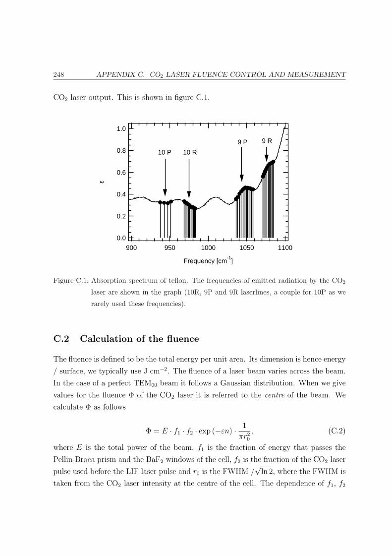
248 APPENDIX C. CO2 LASER FLUENCE CONTROL AND MEASUREMENT
CO2 laser output. This is shown in figure C.1.
1.0
0.8
0.6
0.4
0.2
0.0
ε
110010501000950900
Frequency [cm-1
]
10 P 10 R
9 P 9 R
Figure C.1: Absorption spectrum of teflon. The frequencies of emitted radiation by the CO2
laser are shown in the graph (10R, 9P and 9R laserlines, a couple for 10P as we
rarely used these frequencies).
C.2 Calculation of the fluence
The fluence is defined to be the total energy per unit area. Its dimension is hence energy
/ surface, we typically use J cm−2. The fluence of a laser beam varies across the beam.
In the case of a perfect TEM00 beam it follows a Gaussian distribution. When we give
values for the fluence Φ of the CO2 laser it is referred to the centre of the beam. We
calculate Φ as follows
Φ = E · f1 · f2 · exp (−εn) · 1
πr20
, (C.2)
where E is the total power of the beam, f1 is the fraction of energy that passes the
Pellin-Broca prism and the BaF2 windows of the cell, f2 is the fraction of the CO2 laser
pulse used before the LIF laser pulse and r0 is the FWHM /√
ln 2, where the FWHM is
taken from the CO2 laser intensity at the centre of the cell. The dependence of f1, f2

C.2. CALCULATION OF THE FLUENCE 249
and r0 on the frequency of the CO2 laser are shown in figures C.2 - C.5.
1.0
0.8
0.6
0.4
0.2
0.0
f 1
10801060104010201000980960940
Frequency [cm-1
]
Figure C.2: Amount of transmitted light f1 by the Pellin-Broca prism and the BaF2 windows
of the cell.
The absorption of the CO2 laser light by the Pellin-Broca prism and the BaF2 window
depends smoothly on the CO2 laser frequency. An ad hoc second order polynomial
dependence can be easily fitted to the data points. f1 includes absorption by a Pellin-
Brocca prism just in front of the cell. This is done because of space limitations after
the Pellin-Brocca prism for the measurement of the energy in the laser beam.
The fraction f2 of the laser shot which is effectively used in our experiments lies between
45 and 53%, although no smooth dependence can be observed. For our data analysis
we took the values obtained by doing a linear fit to the experimental data points.
We measure the FWHM by scanning a small slit at the focal point and measuring
the energy let through it as a function of the displacement x. This is shown in figure C.4.
If the beam profile is Gaussian, the measured energy E ′ let through is given by
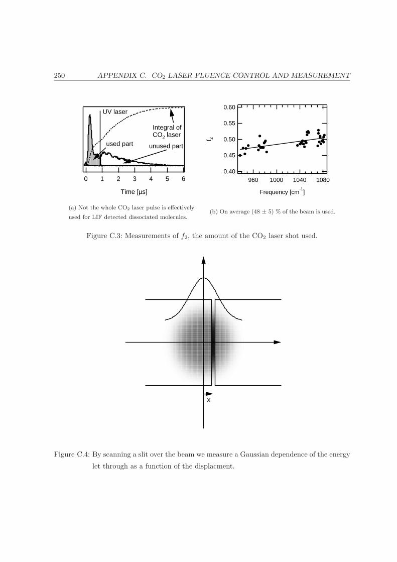
250 APPENDIX C. CO2 LASER FLUENCE CONTROL AND MEASUREMENT
6543210
Time [µs]
used part
UV laser
Integral ofCO2 laser
unused part
(a) Not the whole CO2 laser pulse is effectively
used for LIF detected dissociated molecules.
0.60
0.55
0.50
0.45
0.40
f 2
108010401000960
Frequency [cm-1
]
(b) On average (48 ± 5) % of the beam is used.
Figure C.3: Measurements of f2, the amount of the CO2 laser shot used.
x
Figure C.4: By scanning a slit over the beam we measure a Gaussian dependence of the energy
let through as a function of the displacment.

C.2. CALCULATION OF THE FLUENCE 251
E ′(x) =∞∫−∞
E0·∆xω√
π· exp
(−
((xωx
)2
+(
yωy
)2))
dy
∝ exp
(−
(xωx
)2) (C.3)
and analogous for E ′(y), where E0 is the energy in the total beam, ∆x is the size of the
slit and ωx = 2r0. The widths in the horizontal and vertical directions are not the same,
there is a small distortion because of the Pellin-Broca prism. We show in figure C.5 the
data points we measure.
0.4
0.3
0.2
0.1
0.0
Are
a [m
m2 ]
108010401000960
Frequency [cm-1
]
300
250
200
150
100
50
0
Energy of a single shot [m
J] Area Energy
Figure C.5: Cross-section of the CO2 laser beam at the focal point (left axis) and output
energy of pulse (right axis).
There is a correlation between the area of the focal spot and the total energy of the
laser shot (see figure C.5): the higher the energy of a pulse, the larger the area. We
believe that this is because in the case of a high energy pulse it is not a clean TEM00
pulse. These modes are less well focused than the TEM00 mode, which broadens the
area. As most of the measurements have been done with laser lines at the centre of the
emission bands of the CO2 laser we always use 0.4 mm2 as area.
With the measurements of ε, f1, f2 and r0 as a function of the CO2 laser frequency

252 APPENDIX C. CO2 LASER FLUENCE CONTROL AND MEASUREMENT
we have now all instruments at our hand to accurately calculate the fluence‡ of the CO2
laser radiation.
‡Often called the “effective fluence” if we want to stress the fact that f2, the fraction of the CO2 laser
radiation actually used, is included.
Appendix D
CO2 laser fluence dependence of the
decay rate
There is a surprising effect one can observe: the measured decay rate k as a function
of the dissociation laser fluence goes through a maximum and drops for both the high
fluence and the low fluence limit. We show in figure D.1 an example of how the decay
rate k behaves as a function of the dissociation laser fluence.
The values of the decay rates k in figure D.1 go through a maximum at ∼1 J cm−2. This
behaviour is often observed for different measurements. How can this be explained ?
We give an explanation of this phenomenon.
In a typical experiment where we scan the delay between the pre-excitation and the
dissociation lasers, our system first selectively dissociates pre-excited molecules with
the CO2 laser, then the photofragments are detected via LIF. We do not exclusively
detect molecules still having all their initial vibrational energy at the onset of the dis-
sociation laser, but also molecules having lost a part of it. Because they have lost
vibrational energy, their dissociation probability drops.
We show in figure D.2 qualitatively the dissociation probability for a low, an inter-
mediate and a high fluence of the dissociation laser.
The arrows in the figure show a typical amount of energy a molecule has to lose until the
253

254 APPENDIX D. CO2 LASER FLUENCE DEPENDENCE OF THE DECAY RATE
0.0025
0.0020
0.0015
0.0010
0.0005
0.0000
k [n
s-1 m
bar-1
]
14121086420
Fluence [J cm-2
]
Figure D.1: Example of a measurement of k as a function of the fluence of the dissociation
laser, for the 13CF3H isotopomer pre-excited via the 21 band, at a dissociation
laser frequency of 1047 cm−1, with 75% 13CF3H and 25% 12CF3H in the sample.
dissociation laser does not dissociate them efficiently any more. An “efficient” dissocia-
tion is defined with respect to the dissociation probability at the pre-excitation energy.
It can be seen that the smallest energy window probed by the dissociation laser is not
in the zero fluence limit, but at an intermediate fluence. In both the low and the high
fluence limits the windows grow again. This is a consequence of how the dissociation
probability changes with the vibrational excitation of the molecule.
It turns out, that in general this fluence lies around 1-2 J cm−2.
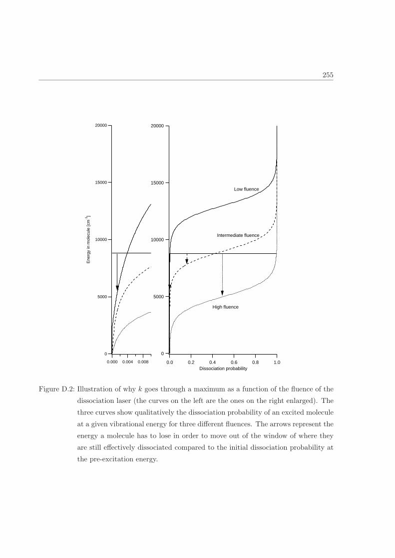
255
20000
15000
10000
5000
0
1.00.80.60.40.20.0Dissociation probability
Low fluence
Intermediate fluence
High fluence
20000
15000
10000
5000
0
Ene
rgy
in m
olec
ule
[cm
-1]
0.0080.0040.000
Figure D.2: Illustration of why k goes through a maximum as a function of the fluence of the
dissociation laser (the curves on the left are the ones on the right enlarged). The
three curves show qualitatively the dissociation probability of an excited molecule
at a given vibrational energy for three different fluences. The arrows represent the
energy a molecule has to lose in order to move out of the window of where they
are still effectively dissociated compared to the initial dissociation probability at
the pre-excitation energy.

256 APPENDIX D. CO2 LASER FLUENCE DEPENDENCE OF THE DECAY RATE

Appendix E
The numerical codes for the
calculation of IRMPD in the
presence of collisions
E.1 Generalities
We show in figure E.1 the rough principle of our code. The code has been written in
fortran 90.
A couple of input files are necessary for the code to work correctly:
1. A file input.files.txt containing the list of files with the description of a single
experiment to calculate (we design one set of pre-excitation, dissociation and LIF
lasers as “one experiment”).
2. The files designated in input.files.txt. These files contain all relevant informa-
tion for the calculations such as the physical parameters (timing of lasers, fluence
of CO2 laser, sample pressure, etc).
3. A file input.rho.txt containing the density of states of CF3H. This has been
calculated by direct counting.
4. A file input.rrkm.txt containing the dissociation rates as calculated by the
RRKM method. This has been calculated with a code from the group around
257
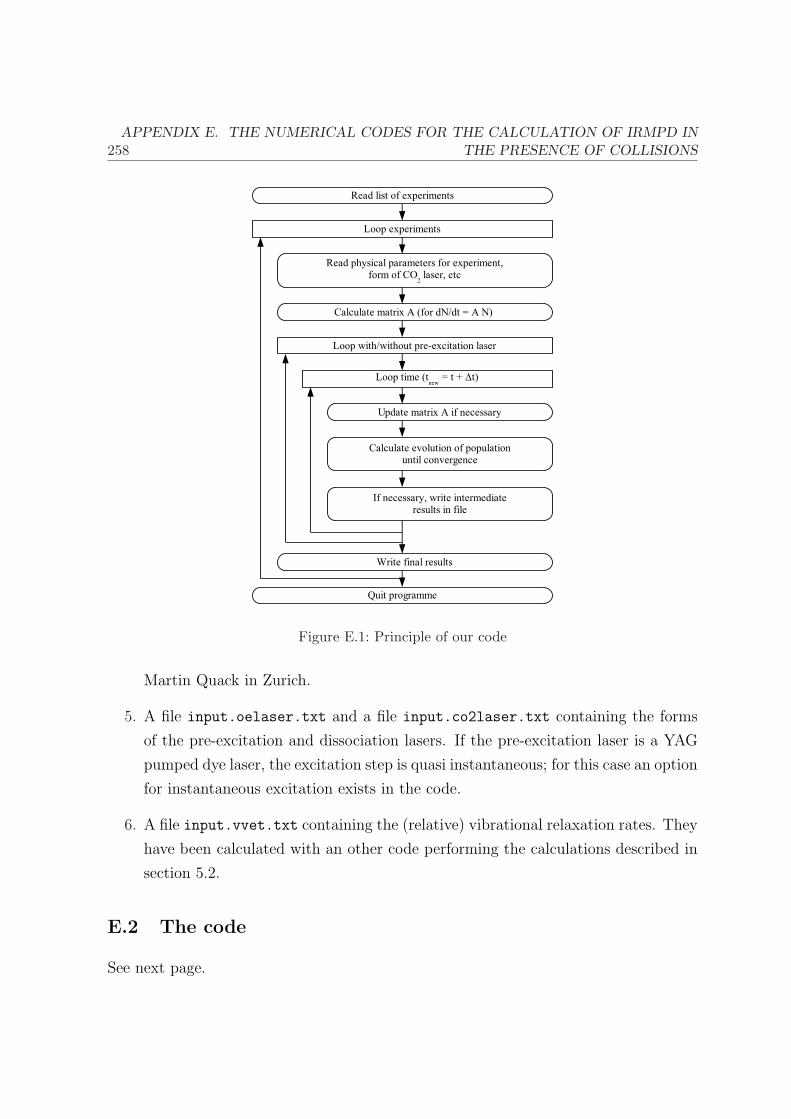
258APPENDIX E. THE NUMERICAL CODES FOR THE CALCULATION OF IRMPD IN
THE PRESENCE OF COLLISIONS
Figure E.1: Principle of our code
Martin Quack in Zurich.
5. A file input.oelaser.txt and a file input.co2laser.txt containing the forms
of the pre-excitation and dissociation lasers. If the pre-excitation laser is a YAG
pumped dye laser, the excitation step is quasi instantaneous; for this case an option
for instantaneous excitation exists in the code.
6. A file input.vvet.txt containing the (relative) vibrational relaxation rates. They
have been calculated with an other code performing the calculations described in
section 5.2.
E.2 The code
See next page.
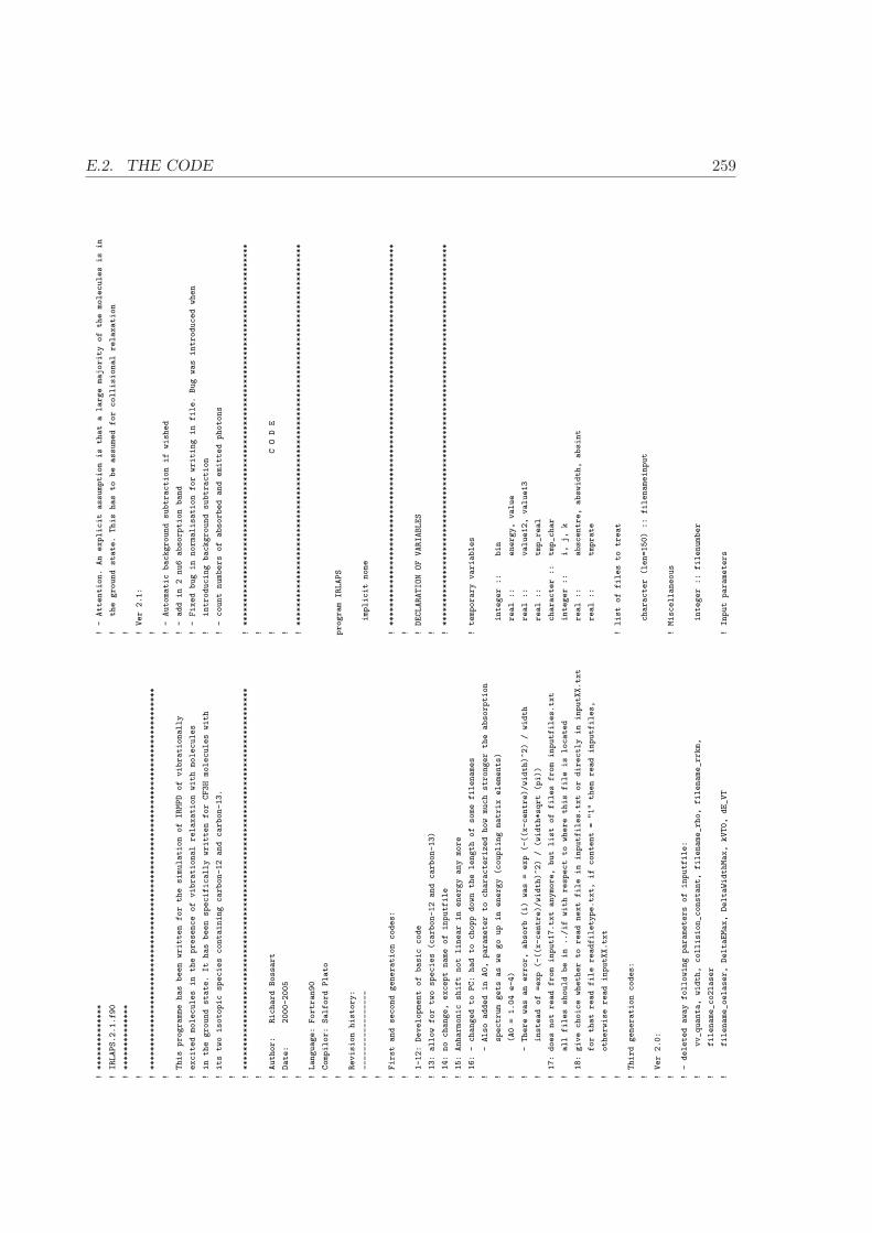
E.2. THE CODE 259
!**************
!IRLAPS.2.1.f90
!**************
! !**********************************************************************************
! !This
programme
has
been
written
for
the
simulation
of
IRMPD
of
vibrationally
!excited
molecules
in
the
presence
of
vibrational
relaxation
with
molecules
!in
the
ground
state.
It
has
been
specifically
written
for
CF3H
molecules
with
!its
two
isotopic
species
containing
carbon-12
and
carbon-13.
! !**********************************************************************************
! !Author:
Richard
Bossart
!Date:
2000-2005
! !Language:
Fortran90
!Compilor:
Salford
Plato
! !Revision
history:
!-----------------
! !First
and
second
generation
codes:
! !1-12:
Development
of
basic
code
!13:
allow
for
two
species
(carbon-12
and
carbon-13)
!14:
no
change,
except
name
of
inputfile
!15:
Anharmonic
shift
not
linear
in
energy
any
more
!16:
-changed
to
PC:
had
to
chopp
down
the
length
of
some
filenames
!-
Also
added
in
A0,
parameter
to
characterized
how
much
stronger
the
absorption
!spectrum
gets
as
we
go
up
in
energy
(coupling
matrix
elements)
!(A0
=1.04
e-4)
!-
There
was
an
error,
absorb
(i)
was
=exp
(-((x-centre)/width)^2)
/width
!instead
of
=exp
(-((x-centre)/width)^2)
/(width*sqrt
(pi))
!17:
does
not
read
from
input17.txt
anymore,
but
list
of
files
from
inputfiles.txt
!all
files
should
be
in
../if
with
respect
to
where
this
file
is
located
!18:
give
choice
whether
to
read
next
file
in
inputfiles.txt
or
directly
in
inputXX.txt
!for
that
read
file
readfiletype.txt,
if
content
="1"
then
read
inputfiles,
!otherwise
read
inputXX.txt
! !Third
generation
codes:
! !Ver
2.0:
! !-
deleted
away
following
parameters
of
inputfile:
!vv_quanta,
width,
collision_constant,
filename_rho,
filename_rrkm,
!filename_co2laser
!filename_oelaser,
DeltaEMax,
DeltaWidthMax,
kVT0,
dE_VT
!-
Attention.
An
explicit
assumption
is
that
alarge
majority
of
the
molecules
is
in
!the
ground
state.
This
has
to
be
assumed
for
collisional
relaxation
! !Ver
2.1:
! !-
Automatic
background
subtraction
if
wished
!-
add
in
2nu6
absorption
band
!-
Fixed
bug
in
normalisation
for
writing
in
file.
Bug
was
introduced
when
!introducing
background
subtraction
!-
count
numbers
of
absorbed
and
emitted
photons
!**********************************************************************************
! !C
OD
E
! !**********************************************************************************
program
IRLAPS
implicit
none
!**********************************************************************************
! !DECLARATION
OF
VARIABLES
! !**********************************************************************************
!temporary
variables
integer
::
bin
real
::
energy,
value
real
::
value12,
value13
real
::
tmp_real
character
::
tmp_char
integer
::
i,
j,
k
real
::
abscentre,
abswidth,
absint
real
::
tmprate
!list
of
files
to
treat
character
(len=150)
::
filenameinput
!Miscellaneous
integer
::
filenumber
!Input
parameters

260APPENDIX E. THE NUMERICAL CODES FOR THE CALCULATION OF IRMPD IN
THE PRESENCE OF COLLISIONS
character(LEN=150)
::
identifier
!Identifier
for
experiment
real::
fl1,
fl2,
fl3,
fl4,
fl5,
fl6,
fl7
!Values
of
physical
parameters
real::
initialt,
finalt
!Timing
real::
photon_energy
!Frequency
of
CO2
laser
real::
fluence
!Fluence
of
CO2
laser
integer::
bins_per_photon
!Bins
per
photon
real::
level_excited
!Pre-excitation
level
real::
fraction_excited1
!Fraction
of
12CF3H
excited
real::
fraction_excited2
!Fraction
of
13CF3H
excited
real::
pressure
!Sample
pressure
integer::
bg_subtr
!1
=automatic
background
subtraction
!otherwise
=no
integer::
instant_excitation
!1
=YAG
laser
!otherwise
=take
profile
from
!filename_oelaser
real::
timedelay1
!Time-delay
between
pre-excitation
and
!CO2
lasers
real::
timedelay2
!Time-delay
between
CO2
and
LIF
lasers
real::
E_max
!Maximum
vibrational
energy
considered
real::
E_lim
!Energy
above
which
the
dissociation
rate
!is
>>
MPA
real::
ratio_max
!Maximum
error
for
calculation
with
!Runge-Kutta
real::
deltaT_min
!Minimum
time-step
[not
incorporated
in
!the
code]
real::
deltaT_max
!Maximum
time-step
integer::
store_general
!1
=store
results
integer::
store_popindiv
!1
=store
population.xxxx.txt
integer::
print_deltaT
!Save
results
every
...
ns
in
file
character(LEN=50)
::
filename_rho
!Filename
with
density
of
states
character(LEN=50)
::
filename_rrkm
!Filename
with
RRKM
values
character(LEN=50)
::
filename_co2laser
!Filename
with
form
of
CO2
laser
character(LEN=50)
::
filename_oelaser
!Filename
with
form
of
pre-excitation
!laser
character(LEN=50)
::
filename_vvet
!Filename
with
vibrational
relaxation
!rates
real::
wa
!(*)
real::
wb
!(*)
real::
E0a1
!(*)
real::
E0a2
!(*)
real::
E0b
!(*)
real::
A0
!(*)
real::
ibi
!Integrated
band
intensity
(ground
state)
real::
amount_species2
!Amount
of
carbon-13
in
the
sample
!(*)
The
absorption
spectrum
of
an
excited
CF3H
molecule
with
avibrational
energy
E
!is:
!\sigma
(\nu)
=(1+A0
\cdot
E)
\cdot
!\frac\exp
\left(
-\left(
\frac\nu-\nu_0\omega\right)^2
\right)
!\omega
\sqrt\pi
!where
!\omega
=wa+wb
\cdot
E
!\nu_0
=E0a
+E0b
\cdot
E
!with
!E0a1
for
carbon-12
!E0a2
for
carbon-13
!If
you
have
problems
reading
\LaTeX,
refer
to
equation
5.7
in
the
thesis
!(and
learn
LaTeX
!!)
!file
’rho.txt’
real,
dimension
(:),
allocatable
::
rho,
rho0
integer,
dimension
(:),
allocatable
::
rho_count,
rho0_count
integer
::
rho_nlines,
rho_nlines0
!file
’rrkm.txt’
real,
dimension
(:),
allocatable
::
rrkm
integer,
dimension
(:),
allocatable
::
rrkm_count
integer
::
rrkm_nlines
!file
’vvet.txt’
real,
dimension
(:),
allocatable
::
vvet
integer,
dimension
(:),
allocatable
::
vvet_count
integer
::
vvet_nlines
!file
’co2laser.txt’
real,
dimension
(:),
allocatable
::
co2laser
real
::
co2laser_dt
integer
::
co2laser_nlines
!file
’OElaser.txt’
real,
dimension
(:),
allocatable
::
oelaser
real
::
oelaser_dt
integer
::
oelaser_nlines
!General
parameters
calculated
from
input
parameters
real
::
dE_bin
!binwidth
integer
::
n!
number
of
levels
real,
dimension
(:),
allocatable
::
absorb
!Absorption
intensity
in
function
!of
the
pre-excitation
energy

E.2. THE CODE 261
!Matrices
A1
real,
dimension
(:,:),
allocatable
::
a1_rrkm,
a1_up,
a1_up_noint,
a1_coll
real,
dimension
(:,:),
allocatable
::
a1_downB,
a1_downC,
a1_downB_noint
real,
dimension
(:,:),
allocatable
::
a1_downC_noint,
a1_down
real,
dimension
(:,:),
allocatable
::
a1_oe_noint,
a1_oe
real,
dimension
(:,:),
allocatable
::
a1_1,
a1_2,
a1_3,
a1_4,
a1_5
real
::
co2laser_value,
oelaser_value
real
::
co2laser_value_store,
oelaser_value_store
!Calculation
of
timeevolution
real,
dimension
(:),
allocatable
::
pop,
pop1,
pop2,
pop3,
pop4,
newpop,
poptot
real,
dimension
(:),
allocatable
::
pop_onestep,
pop_twosteps,
error_pop
real
::
co2laser_position,
oelaser_position
integer
::
changes_matrix
real
::
co2_intensity
real
::
deltat
real
::
ratio
integer
::
lastprinttime
real
::
time
integer
::
oe_excitation_done
integer
::
bg
!Dissociationprobability
real
::
d12,
d13
!**********************************************************************************
! !INTERFACE
FOR
FUNCTIONS
! !**********************************************************************************
interface
functionderiv
(a1,
pop)
real,
intent
(in),
dimension
(:)
::
pop
real,
intent
(in),
dimension
(:,:)
::
a1
real,
dimension
(1:size(pop))
::
deriv
endfunction
deriv
functioninttochar
(i)
integer,
intent(in)
::
i
character
(LEN=10)
::
inttochar
endfunction
inttochar
end
interface
!**********************************************************************************
! !BEGIN
CODE
! !**********************************************************************************
write
(*,*)
write
(*,*)
"**********************"
write
(*,*)
"*
Running
simulation
*"
write
(*,*)
"**********************"
write
(*,*)
!**********************************************************************************
! !Read
input
file
! !**********************************************************************************
filenumber
=0
open
(16,
file="input.files.txt",
status="old")
do
filenumber=
filenumber
+1
read(16,*)
filenameinput
if(trim
(filenameinput)
==
"NOFILESLEFTOVER")
exit
write(*,*)
"File
:"
//
trim
(filenameinput)
open(10,
file="inputfiles/"
//
trim
(filenameinput),
status="old")
!Identification
read(10,
*)
fl1,
fl2,
fl3,
fl4,
fl5,
fl6,
fl7
read(10,
*)
identifier
!Physical
properties
read(10,
*)
photon_energy
read(10,
*)
fluence
read(10,
*)
pressure
read(10,
*)
amount_species2
read(10,
*)
level_excited
read(10,
*)
fraction_excited1
read(10,
*)
fraction_excited2
read(10,
*)
instant_excitation
!Background
substraction
read(10,
*)
bg_subtr
!timing
read(10,
*)
initialt
read(10,
*)
timedelay2
read(10,
*)
timedelay1
!Absorption
spectrum
of
excited
state
262APPENDIX E. THE NUMERICAL CODES FOR THE CALCULATION OF IRMPD IN
THE PRESENCE OF COLLISIONS
read
(10,
*)
wa
read
(10,
*)
wb
read
(10,
*)
E0a1
read
(10,
*)
E0a2
read
(10,
*)
E0b
read
(10,
*)
A0
read
(10,
*)
ibi
!Numerical
details
read
(10,
*)
ratio_max
read
(10,
*)
deltaT_min
read
(10,
*)
deltaT_max
read
(10,
*)
E_max
read
(10,
*)
E_lim
read
(10,
*)
bins_per_photon
!output
in
file
read
(10,
*)
store_general
read
(10,
*)
store_popindiv
read
(10,
*)
print_deltaT
close
(10)
if
(bg_subtr
/=
1)
bg_subtr
=0
filename_rho
="input.rho.txt"
filename_rrkm
="input.rrkm.txt"
filename_co2laser
="input.co2laser.txt"
filename_oelaser
="input.oelaser.txt"
filename_vvet
="input.vvet.txt"
!**********************************************************************************
! !CALCULATE
PARAMETERS
NECESSARY
FOR
THE
SIMULATIONS,
AND
LOAD
EXTERNAL
FILES
! !**********************************************************************************
dE_bin
=photon_energy
/bins_per_photon
n=
int
(E_max/dE_bin)
+1
finalt
=timedelay1
+timedelay2
allocate
(rho
(0:2*n-1))
allocate
(rho0
(0:2*n-1))
allocate
(rho_count
(0:2*n-1))
allocate
(rho0_count
(0:2*n-1))
allocate
(rrkm
(0:2*n-1))
allocate
(rrkm_count
(0:2*n-1))
allocate
(vvet
(0:2*n-1))
allocate
(vvet_count
(0:2*n-1))
allocate
(absorb
(0:2*n-1))
rho=
0.
rho0=
0.
rho_count=
0
rho0_count=
0
rrkm=
0.
rrkm_count=
0
vvet=
0.
vvet_count=
0
absorb=
0.
!Density
of
states
open(10,
file=trim(filename_rho),
status="old")
read(10,
*)
tmp_char
read(10,
*)
tmp_char
read(10,
*)
tmp_char
read(10,
*)
rho_nlines
doi=1,
rho_nlines
read
(10,
*)
energy,
value
energy
=energy
*1000
bin
=int(energy/dE_bin)
if
(bin
<n)
then
rho
(bin)
=rho
(bin)
+10**value
rho_count
(bin)
=rho_count
(bin)
+1
endif
enddo
read(10,
*)
rho_nlines0
doi=1,
rho_nlines0
read
(10,
*)
energy,
value
energy
=energy
*1000
bin
=int(energy/dE_bin)
if
(bin
<n)
then
rho0
(bin)
=rho0
(bin)
+10**value
rho0_count
(bin)
=rho0_count
(bin)
+1
endif
enddo
close(10)
where(rho_count
/=
0)
rho
=rho
/rho_count
where(rho0_count
/=
0)
rho0
=rho0
/rho0_count
deallocate(rho_count)
deallocate(rho0_count)
E.2. THE CODE 263
rho(n:2*n-1)
=rho
(0:n-1)
rho0(n:2*n-1)
=rho0
(0:n-1)
!RKKM
dissociation
open(10,
file=trim(filename_rrkm),
status="old")
read(10,
*)
rrkm_nlines
doi=1,
rrkm_nlines
read
(10,
*)
energy,
value
bin
=int(energy/dE_bin)
if
(bin
<n)
then
rrkm
(bin)
=rrkm
(bin)
+value
rrkm_count
(bin)
=rrkm_count
(bin)
+1
endif
enddo
close(10)
where(rrkm_count
/=
0)
rrkm
=rrkm
/rrkm_count
rrkm=
rrkm
/10E9
deallocate(rrkm_count)
rrkm(n:2*n-1)
=rrkm
(0:n-1)
!V-V
energy
transfer
open(10,
file=trim(filename_vvet),
status="old")
read(10,
*)
vvet_nlines
doi=1,
vvet_nlines
read
(10,
*)
energy,
value12,
value13
bin
=int(energy/dE_bin)
if
(bin
<n)
then
vvet
(bin)
=vvet
(bin)
+value12
vvet
(bin+n)
=vvet
(bin+n)
+value13
vvet_count
(bin)
=vvet_count
(bin)
+1
vvet_count
(bin+n)
=vvet_count
(bin+n)
+1
endif
enddo
close(10)
where(vvet_count
/=
0)
vvet
=vvet
/vvet_count
vvet=
vvet
*1e-3
deallocate(vvet_count)
!Calculate
relative
absorption
strengths
doi=0,
n-1
energy
=(i+0.5)*dE_bin
abscentre
=E0a1
+E0b
*energy
abswidth
=sqrt
(wa**2
+(wb
*energy)**2)
absint
=(1
+a0
*energy)
absorb
(i)
=absint
*exp
(-
(((
photon_energy
-abscentre
)/
abswidth
)**2))&
/(abswidth*sqrt(3.1415))
!Absorption
by
2nu6
abscentre
=1024.1
-0.0039206
*energy
abswidth
=sqrt
(wa**2
+(3.9256
+0.0024206
*energy)**2)
absint
=(5.0253e-5
*energy
+3.8577e-9
*energy
*energy)
/0.0282095
absorb
(i)
=absorb
(i)
+&
2.75e-4*absint*
exp
(-
(((
photon_energy
-abscentre
)/
abswidth
)**2))
&
/(abswidth*sqrt(3.1415))
enddo
doi=n,
2*n-1
energy
=((i-n)+0.5)*dE_bin
abscentre
=E0a2
+E0b
*energy
abswidth
=sqrt
(wa**2
+(wb
*energy)**2)
absint
=(1
+a0
*energy)
absorb
(i)
=absint
*exp
(-
(((
photon_energy
-abscentre
)/
abswidth
)**2))&
/(abswidth*sqrt(3.1415))
!Absorption
by
2nu6
abscentre
=1024.1
-0.0039206
*energy
abswidth
=sqrt
(wa**2
+(3.9256
+0.0024206
*energy)**2)
absint
=(5.0253e-5
*energy
+3.8577e-9
*energy
*energy)
/0.0282095
absorb
(i)
=absorb
(i)
+&
2.75e-4*absint
*exp
(-
(((
photon_energy
-abscentre
)/
abswidth
)**2))
&
/(abswidth*sqrt(3.1415))
enddo
!Read
CO2
laser
profile
open(10,
file=trim(filename_co2laser),
status="old")
read(10,
*)
co2laser_nlines,
co2laser_dt
allocate(co2laser
(0:co2laser_nlines-1))
264APPENDIX E. THE NUMERICAL CODES FOR THE CALCULATION OF IRMPD IN
THE PRESENCE OF COLLISIONS
do
i=
0,
co2laser_nlines-1
read(10,
*)
tmp_real,
co2laser
(i)
enddo
co2laser
=co2laser
/sum
(co2laser)
close
(10)
!Read
pre-excitation
laser
profile
(for
PAL
laser)
open
(10,
file=trim(filename_oelaser),
status="old")
read
(10,
*)
oelaser_nlines,
oelaser_dt
allocate
(oelaser
(0:oelaser_nlines-1))
do
i=
0,
oelaser_nlines-1
read(10,
*)
tmp_real,
oelaser
(i)
enddo
oelaser
=oelaser
/sum
(oelaser)
close
(10)
!**********************************************************************************
! !Calculate
Matrices
! !**********************************************************************************
allocate
(A1_rrkm
(0:2*n-1,0:2*n-1))
allocate
(A1_up_noint
(0:2*n-1,0:2*n-1))
allocate
(A1_downB_noint
(0:2*n-1,0:2*n-1))
allocate
(A1_downC_noint
(0:2*n-1,0:2*n-1))
allocate
(a1_oe_noint
(0:2*n-1,0:2*n-1))
allocate
(a1_coll
(0:2*n-1,0:2*n-1))
A1_rrkm
=0.
A1_up_noint
=0.
A1_downB_noint
=0.
A1_downC_noint
=0.
a1_oe_noint
=0.
a1_coll
=0.
!Pre-excitation
matrix
a1_oe_noint(int(level_excited/dE_bin),0)
=fraction_excited1
a1_oe_noint(0,0)
=-
a1_oe_noint(int(level_excited/dE_bin),0)
a1_oe_noint(n+int(level_excited/dE_bin),n)=
fraction_excited2
a1_oe_noint(n,n)=
-a1_oe_noint(n+int(level_excited/dE_bin),n)
if(instant_excitation
==
1)
a1_oe_noint
=0.
!RRKM
matrix
doi=0,
n-1
a1_rrkm(i,i)
=-
rrkm
(i)
a1_rrkm(i+n,i+n)
=-
rrkm
(i)
enddo
!Uppumping
matrix
doi=0,
2*n-1
if
(rho
(i)
/=
0.)
then
a1_up_noint(i,i)
=-
1.511
*ibi
*absorb
(i)
*rho0
(i)
/rho
(i)
if
(i<=n-1-bins_per_photon)
&
a1_up_noint(i+bins_per_photon,i)=
-a1_up_noint(i,i)
if
((i<2*n-1-bins_per_photon).and.(i>=n))
&
a1_up_noint(i+bins_per_photon,i)=
-a1_up_noint(i,i)
endif
enddo
!Downpumping
matrix
case
B(high
density
of
states)
doi=bins_per_photon,
2*n-1
if
(rho(i)/=0.)
then
if
((i<=n-1).or.(i>=n+bins_per_photon))
then
A1_downB_noint(i,i)=
-1.511
*ibi
*rho0
(i-bins_per_photon)
&
*absorb
(i-bins_per_photon)
/rho
(i)
A1_downB_noint(i-bins_per_photon,i)=
-A1_downB_noint(i,i)
endif
endif
enddo
!Downpumping
matrix
case
C(low
density
of
states)
doi=bins_per_photon,
2*n-1
if
((rho
(i-bins_per_photon)/=0.).and.(rho(i)/=0.).and.
&
(rho0(i-bins_per_photon)/=0.))
then
if
((i<=n-1).or.(i>=n+bins_per_photon))
then
A1_downC_noint(i,i)=
-(2./
(3.141592
*(3**0.5))
)*
&
(1.511
*ibi
*absorb
(i-bins_per_photon)
&
*rho0
(i-bins_per_photon)
*rho
(i-bins_per_photon)
/&
(rho
(i)**3)
)**0.5

E.2. THE CODE 265
A1_downC_noint(i-bins_per_photon,i)
=-
A1_downC_noint(i,i)
endif
endif
enddo
!V-V
Energy
transfer
doi=bins_per_photon,
2*n-1
if
((i<=n-1).or.(i>=n+bins_per_photon))
then
!Assume
large
majority
of
molecules
in
gs
A1_coll(i,i)
=-
vvet
(i)
*pressure
A1_coll(i-bins_per_photon,i)
=-
A1_coll(i,i)
a1_coll(0,i)
=a1_coll(0,i)
+A1_coll(i,i)
!Assume
large
majority
of
molecules
C12
a1_coll(bins_per_photon,i)
=a1_coll(bins_per_photon,i)
-A1_coll(i,i)
endif
enddo
!**********************************************************************************
! !Perform
calculations
! !**********************************************************************************
!Initialise
variables
allocate(pop
(0:2*n-1))
allocate(newpop
(0:2*n-1))
allocate(pop1
(0:2*n-1))
allocate(pop2
(0:2*n-1))
allocate(pop3
(0:2*n-1))
allocate(pop4
(0:2*n-1))
allocate(pop_onestep
(0:2*n-1))
allocate(pop_twosteps
(0:2*n-1))
allocate(error_pop
(0:2*n-1))
allocate(a1_1
(0:2*n-1,0:2*n-1))
allocate(a1_2
(0:2*n-1,0:2*n-1))
allocate(a1_3
(0:2*n-1,0:2*n-1))
allocate(a1_4
(0:2*n-1,0:2*n-1))
allocate(a1_5
(0:2*n-1,0:2*n-1))
allocate(a1_up
(0:2*n-1,0:2*n-1))
allocate(a1_downB
(0:2*n-1,0:2*n-1))
allocate(a1_downC
(0:2*n-1,0:2*n-1))
allocate(a1_down
(0:2*n-1,0:2*n-1))
allocate(a1_oe
(0:2*n-1,0:2*n-1))
allocate(poptot
(0:2*n-1))
!**********************************************************************************
! !Loop:
with/without
pre-excitation
laser
! !**********************************************************************************
dobg=0,
bg_subtr
if
(bg==1)
then
fraction_excited1=
0.
fraction_excited2=
0.
a1_oe_noint=
0.
endif
!**********************************************************************************
! !Initialisations
! !**********************************************************************************
pop
=0.
pop
(0)
=1.-amount_species2
pop
(n)
=amount_species2
time
=initialt
lastprinttime
=int
((time-initialt)
/print_deltaT)
-1
deltat
=1.
oe_excitation_done
=0
if
(store_general
==
1)
then
if(bg
==
0)
then
open
(20,
file="results/p."
//
trim(identifier)
//
".txt")
else open
(20,
file="results/p.bg."
//
trim(identifier)
//
".txt")
endif
endif
!**********************************************************************************
! !Loop:
time
evolution
! !**********************************************************************************
266APPENDIX E. THE NUMERICAL CODES FOR THE CALCULATION OF IRMPD IN
THE PRESENCE OF COLLISIONS
do
do
!Check
whether
any
matrices
have
to
be
updated
doi=1,
5
co2laser_position
=(time+(1.*(i-1)*deltat/4.)-timedelay1)
/co2laser_dt
oelaser_position
=(time+(1.*(i-1)*deltat/4.))
/oelaser_dt
if
((co2laser_position>0.).and.&
(co2laser_position<1.*(co2laser_nlines-1)))
&
then co2laser_value=
(co2laser_position
-1.*int
(co2laser_position))
&
*co2laser
(int(co2laser_position)+1)
+(1.
+&
1.*int(co2laser_position)
-co2laser_position)
*&
co2laser(int(co2laser_position))
else co2laser_value
=0.
endif
if
((oelaser_position>0.).and.(oelaser_position<1.*(oelaser_nlines-1)))
&
then
changes_matrix
=1
oelaser_value
=(oelaser_position
-1.*int
(oelaser_position))
&
*oelaser
(int(oelaser_position)+1)
+(1.
+&
1.*int(oelaser_position)
-oelaser_position)
*&
oelaser(int(oelaser_position))
else oelaser_value
=0.
endif
if
(i==3)
then
co2laser_value_store
=co2laser_value
oelaser_value_store
=oelaser_value
endif
co2_intensity
=fluence
*co2laser_value
/(co2laser_dt*1E-9*1E6)
!Check
a1_up
=a1_up_noint
*co2_intensity
a1_downB
=a1_downB_noint
*co2_intensity
a1_downC
=a1_downC_noint
*sqrt(co2_intensity)
a1_down
=a1_downB
do
j=0,
n-1
do
k=0,1
if
(abs
(A1_downC
(k*n+j,k*n+j))
>abs
(A1_downB
(k*n+j,k*n+j)))
&
then
A1_down
(k*n+j,k*n+j)
=A1_downC
(k*n+j,k*n+j)
A1_down
(k*n+j-bins_per_photon,k*n+j)
=&
A1_downC
(k*n+j-bins_per_photon,k*n+j)
if
(pop
(k*n+j)
>pop
(k*n+j-bins_per_photon))
then
!Generalisation
case
C
tmprate
=A1_up
(k*n+j-bins_per_photon,k*n+j-bins_per_photon)
A1_up
(k*n+j-bins_per_photon,k*n+j-bins_per_photon)
=&
A1_down
(k*n+j,k*n+j)
A1_down
(k*n+j,
k*n+j)
=tmprate
tmprate
=A1_up
(k*n+j,k*n+j-bins_per_photon)
A1_up
(k*n+j,k*n+j-bins_per_photon)
=&
A1_down
(k*n+j-bins_per_photon,k*n+j)
A1_down
(k*n+j-bins_per_photon,
k*n+j)
=tmprate
endif
endif
enddo
enddo
a1_oe
=a1_oe_noint
*oelaser_value
/oelaser_dt
if
(i==1)
a1_1
=a1_oe
+a1_up
+a1_down
+a1_rrkm
+a1_coll
if
(i==2)
a1_2
=a1_oe
+a1_up
+a1_down
+a1_rrkm
+a1_coll
if
(i==3)
a1_3
=a1_oe
+a1_up
+a1_down
+a1_rrkm
+a1_coll
if
(i==4)
a1_4
=a1_oe
+a1_up
+a1_down
+a1_rrkm
+a1_coll
if
(i==5)
a1_5
=a1_oe
+a1_up
+a1_down
+a1_rrkm
+a1_coll
enddo
!Do
calculation
RUNGE-KUTTA
pop1=
deltat
*deriv
(a1_1,
pop)
pop2=
deltat
*deriv
(a1_3,
pop+0.5*pop1)
pop3=
deltat
*deriv
(a1_3,
pop+0.5*pop2)
pop4=
deltat
*deriv
(a1_5,
pop+pop3)
pop_onestep=
pop
+(pop1
+2.*(pop2+pop3)
+pop4)
/6.
pop1=
pop1
/2.
pop2=
deltat
*deriv
(a1_2,pop+0.5*pop1)
/2.
pop3=
deltat
*deriv
(a1_2,pop+0.5*pop2)
/2.
pop4=
deltat
*deriv
(a1_3,pop+pop3)
/2.
pop_twosteps=
pop
+(pop1
+2.*(pop2+pop3)
+pop4)
/6.
pop1=
deltat
*deriv
(a1_3,pop_twosteps)
/2.
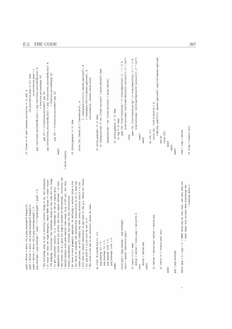
E.2. THE CODE 267
pop2
=deltat
*deriv
(a1_4,pop_twosteps+0.5*pop1)/2.
pop3
=deltat
*deriv
(a1_4,pop_twosteps+0.5*pop2)/2.
pop4
=deltat
*deriv
(a1_5,pop_twosteps+pop3)
/2.
pop_twosteps
=pop_twosteps
+(pop1
+2.*(pop2+pop3)
+pop4)
/6.
!The
following
step
is
not
astrictly
correct
thing
to
do,
but
necessary
!It
turns
out
that
for
high
Energies,
where
RRKM
values
>>
other
values
!(IR
pumping,
collisions)
the
timesteps
chosen
by
the
code
are
too
large
!to
get
consistent
results.
(i.e.
timesteps
in
the
ns
region
give
!apparently
values
which
are
within
the
error
region
defined
-in
fact
!the
values
for
N_i
grow
for
high
Einstead
of
decreasing).
Correctly
one
!should
advance
with
much
smaller
time
steps
(e.g.
0.001
ns),
but
this
!would
considerably
increase
the
time
for
the
calculations.
!We
chose
amore
pragmatic
approach:
by
defining
acertain
value
e_lim
!for
which
we
consider
the
unimolecular
dissociation
to
be
>>
than
any
!other
process,
we
will
simply
say
that
every
molecule
with
E>
e_lim
!will
have
no
chance
whatsoever
to
get
down
to
the
g.s.
Hence
all
values
!for
pop
with
E>
e_lim
will
be
set
to
0.
!The
value
e_lim
has
to
be
carefully
chosen
by
hand.
do
i=int
(E_lim/dE_bin)+1,
n-1
pop_onestep
(i)
=0.
pop_twosteps
(i)
=0.
pop_onestep
(i+n)
=0.
pop_twosteps
(i+n)
=0.
enddo
error_pop
=(pop_onestep
-pop_twosteps)
ratio
=maxval
(abs(error_pop))
if
(ratio
/=
0.)
then
deltat
=deltat
*(ratio_max
/ratio)**0.2
else deltat
=deltat_max
endif
if
(deltat
>deltat_max)
deltat
=deltat_max
if
(ratio
<=
1.1*ratio_max)
exit
enddo
pop
=pop_twosteps
!where
(pop
<0.)
pop
=0.
!RRKM
rates
may
be
very
fast,
and
they
have
not
!been
taken
into
account
when
evaluating
the
!timestep
delta
t.
if((time
>=
0).and.(instant_excitation
==
1).and.
&
(oe_excitation_done
==
0))
then
oe_excitation_done
=1
pop
(int(level_excited/dE_bin))
=pop
(int(level_excited/dE_bin))
&
+fraction_excited1*pop
(0)
pop
(0)
=(1-fraction_excited1)*
pop
(0)
pop
(n+int(level_excited/dE_bin))
=pop
(n+int(level_excited/dE_bin))
&
+fraction_excited2*pop
(n)
pop
(n)
=(1-fraction_excited2)*
pop
(n)
endif
!Write
results
if(store_general
==
1)
then
write
(20,’(5es15.5)’)
time+deltat/2.,
&
1.-(sum(pop(0:n-1))/(1.-amount_species2)),
&
1-(sum(pop(n:2*n-1))/amount_species2),
&
co2_intensity,
oelaser_value_store
if
(store_popindiv
==
1)
then
if(lastprinttime
/=
int
((time-initialt)
/print_deltaT))
then
lastprinttime
=int
((time-initialt)
/print_deltaT)
if
(store_general
==
1)
then
if
(bg
==
0)
then
open(21,
file="results/p."
//
trim(identifier)
//
"."
//
&
trim(inttochar
(int(time+(deltat/2)-initialt)))
//
".txt")
else open(21,
file="results/p.bg."
//
trim(identifier)
//
"."
//
&
trim(inttochar
(int(time+(deltat/2)-initialt)))
//
".txt")
endif
endif
do
i=0,
n-1
write
(21,
’(f15.5,2e14.5)’)
&
i*dE_bin,pop(i)/(1.-amount_species2),
pop(i+n)/amount_species2
end
do
close
(21)
endif
endif
endif
time=
time
+deltat
if(time
>finalt)
exit

268APPENDIX E. THE NUMERICAL CODES FOR THE CALCULATION OF IRMPD IN
THE PRESENCE OF COLLISIONS
enddo
if(store_general
==
1)
close
(20)
if(bg==0)
poptot
=pop
enddo
!**********************************************************************************
! !Write
final
results
! !**********************************************************************************
if
(bg_subtr==0)
then
d12=
1.-(sum(pop(0:n-1))/(1.-amount_species2))
d13=
1.-(sum(pop(n:2*n-1))/amount_species2)
else d12=
(sum(pop(0:n-1))-sum(poptot(0:n-1)))/(1.-amount_species2)
d13=
(sum(pop(n:2*n-1))-sum(poptot(n:2*n-1)))/amount_species2
endif
if
(filenumber
==
1)
then
open(20,
file="results/d.all.txt")
else open(20,
file="results/d.all.txt",
position="append")
endif
write
(20,*)
fl1,
fl2,
fl3,
fl4,
fl5,
fl6,
fl7,
d12,
d13
close
(20)
!**********************************************************************************
! !END
! !**********************************************************************************
deallocate
(rho)
deallocate
(rho0)
deallocate
(rrkm)
deallocate
(absorb)
deallocate
(co2laser)
deallocate
(A1_rrkm)
deallocate
(A1_up_noint)
deallocate
(A1_downB_noint)
deallocate
(A1_downC_noint)
deallocate
(pop)
deallocate(A1_up)
deallocate(A1_downB)
deallocate(A1_downC)
deallocate(A1_down)
deallocate(oelaser)
deallocate(a1_oe_noint)
deallocate(newpop)
deallocate(pop1)
deallocate(pop2)
deallocate(pop3)
deallocate(pop4)
deallocate(pop_onestep)
deallocate(pop_twosteps)
deallocate(error_pop)
deallocate(a1_1,
a1_2,
a1_3,
a1_4,
a1_5)
deallocate(a1_oe)
deallocate(vvet)
deallocate(a1_coll)
deallocate(poptot)
enddo
close
(16)
endprogram
IRLAPS
!**********************************************************************************
! !FUNCTIONS
! !**********************************************************************************
functionderiv
(a1,pop)
implicit
none
real,
intent
(in),
dimension
(:)
::
pop
real,
intent
(in),
dimension
(:,:)
::
a1
real,
dimension
(1:size(pop))
::
deriv
integer
::
n
n=size(pop)
deriv
=matmul
(a1,
pop)
endfunction
deriv
functioninttochar
(i)
integer,
intent(in)
::
i
integer
::
i_part

E.2. THE CODE 269
character
::
i_part_char
character
(LEN=10)
::
inttochar,
inttocharp
integer
::
j,
dim,
ip
ip
=i
if
(i
>0)
then
dim=
1+int
(log10
(ip*1.0))
inttocharp=
""
doj=1,
4-dim
inttocharp
=trim(inttocharp)
//
"0"
enddo
doj=1,
dim
i_part
=int
(ip/(10**(dim-j)))
ip
=int
(ip
-(10**(dim-j))*i_part)
select
case
(i_part)
case
(1)
i_part_char
="1"
case
(2)
i_part_char
="2"
case
(3)
i_part_char
="3"
case(4)
i_part_char
="4"
case(5)
i_part_char
="5"
case(6)
i_part_char
="6"
case(7)
i_part_char
="7"
case(8)
i_part_char
="8"
case(9)
i_part_char
="9"
case(0)
i_part_char
="0"
end
select
inttocharp
=trim(inttocharp)
//
i_part_char
enddo
else inttocharp=
"0000"
endif
inttochar
=inttocharp
end
function
inttochar

270APPENDIX E. THE NUMERICAL CODES FOR THE CALCULATION OF IRMPD IN
THE PRESENCE OF COLLISIONS

Notations, constants and
abbreviations
Notations and constants
~d Dipole moment Eq. 5.22
dhs Hard sphere diameter Eq. 2.47
f Fraction of 13CF3H in sample Section 4.5.2
f1 Amount of transmitted light by optical sys-
tem, for dissociation laser
Eq. C.2, fig.
C.2
f2 Amount of pulse used for the dissociation of
molecules
Eq. C.2, fig.
C.3
gtt′ Anharmonicity constants Eq. 2.2, table
2.3
gi Degeneracy of a vibrational mode i Eq. 5.8
h Planck constant ∼6.626 ·10−34 J s
k Decay rate
k k · pxk Pumping rates for calculations due to x Section 5.3.2
kB Boltzmann constant ∼1.380 ·10−23 J K−1
n Amount of teflon sheets used Eq. C.1
〈n〉 Average occupation number in a mode Eq. 5.8
p Pressure
Continued on next page
271

272 NOTATIONS, CONSTANTS AND ABBREVIATIONS
Notations and constants
p Change of bins per absorbed / emitted pho-
ton (calculations)
Section 5.3.1
pI Population of grained level I Table 2.11
q Quenching constant Eq. B.1
q Vibrational coordinate operator
q6 Interaction constant Eq. 5.11
r Distance between molecules Eq. 2.34
r0 Radius of dissociation laser in focal point Eq. C.2, fig.
C.5
r0 Impact parameter in collisions (closest dis-
tance)
Eq. 2.38
rc See definition → Eq. 2.42
rhs Hard sphere radius Eq. 2.42
s Number of oscillators in a molecule Eq. 5.8
s′ Number of independent oscillators in a
molecule
Eq. 5.8
∆t Time-delay between pre-excitation and dis-
sociation lasers (∆tPE−IRMPD) and dissocia-
tion and LIF lasers (∆tIRMPD−LIF )
v Relative velocity of two molecules Eq. 2.30
v Set of vibrational quantum numbers
(v1, v2, . . . , v6)
Page 23
vx Quantum number in mode x
xij Anharmonicity constants Eq. 2.2, table
2.3
x, y See definition → Fig. 2.11
A Increase of integral absorption strength upon
excitation of molecule
Eq. 5.36
AKJ Honl-London factors Eq. 5.13
Ap Integral absorption strength of absorption
spectrum of an excited molecule
Eq. 5.7
Continued on next page

273
Notations and constants
A1, A2 Matrices for master equation calculations Eq. 5.47
B Rotational constant Eq. 2.13
C Rotational constant Eq. 2.13
D Dissociation probability
D Off-resonance shift for photon absorption Page 238
E Enhancement of selectivity Eq. 1.2
E Energy
∆E Width of a bin for the calculations Section 5.3.1
Ed Cut-off level over which dissociation is com-
plete
Page 199
ETS Energy of the transition state Section
5.3.3.C
~E Electrical field Eq. 2.20
F Rotational energy Eq. 2.13
FX Rovibrational absorption spectrum of
molecule X
Eq. 2.46
F See definition → Section A.2,
eq. A.5
G See definition → Section A.2,
eq. A.5
G Integrated band intensity Eq. 2.1
H Molecular Hamiltonian Eq. 2.19
I Intensity of dissociation laser Eq. 2.27, eq.
5.54
J Rotational quantum number Eq. 2.13
K Rotational quantum number Eq. 2.13
KI,J Transition rate from level I to level J Table 2.11
Kp Relaxation rate in collisional quenching Eq. B.1
M Rotational quantum number Page 167
P (E, E ′)Energy transfer probability from E ′ → E Page 61
Continued on next page

274 NOTATIONS, CONSTANTS AND ABBREVIATIONS
Notations and constants
P Probability that a head-on collision results in
energy transfer
Page 182
Pif Transition probability Eq. 2.30
P Number of pre-excited molecules Eq. 4.3
Q Set of vibrational coordinate operators
R Scaling factor for collisional relaxation Section
5.3.3.B
Rc Impact parameter of collision Fig. 5.5
R0 Cut-off distance between two molecules,
where dipole-dipole interaction stop prevail-
ing
Page 167
RAB Distance between two molecules Eq. 2.46
S Dissociation selectivity Eq. 1.1
SIRMPD Dissociation selectivity due to isotopically se-
lective IRMPD
Section
5.3.4.C
SV ET Dissociation selectivity due to isotopically se-
lective collisional relaxation
Section
5.3.4.C
T Temperature
V Coupling between levels Table 2.11
Vd Interaction energy due to dipole-dipole inter-
actions
Eq. 5.22
W Average coupling between two states
W Transition rate Eq. 5.17
W Coupling between states Page 36
Wf Interaction constant Eq. 5.11
Y Dissociation yield
Zhs Hard sphere collision rate Eq. 2.47
α See definition → Eq. 2.14
α See definition → Eq. 2.51
δI Spacing between individual levels in grained
level I
Table 2.11
Continued on next page

275
Notations and constants
δpi Kronecker symbol
δ Width of a gaussian
δ Density of effectively coupled states Page 240
η Transmission of LIF signal through the de-
tection system
Page 108
ε Dissociation efficiency (rotational relaxation) Eq. 3.3
ε Absorption coefficient of teflon Eq. C.1, fig.
C.1
ε0 Permittivity of free space ∼ 8.85 · 10−12
C2 N−1 m−2
κ relaxation rate
κ κ · pω Energy of a photon Table 2.11
ω Width of absorption spectrum
ω Fundamental frequencies Eq. 2.2, table
2.3
ωTS Vibrational frequencies at the transition
state
Table 5.2
µ Reduced mass Eq. 2.30
µ Transition dipole moment (|〈1 |~d| 2〉|) Pages 21 and
60
ν Frequency of a laser
νx Vibrational mode x
νp Pumped vibration
ν0 Band origin
δνp Width of absorption feature of an excited
molecule
Eq. 5.7
∆νp Shift of absorption feature of an excited
molecule
Eq. 5.7
∆ν Linewidth of a laser Page 36
Continued on next page
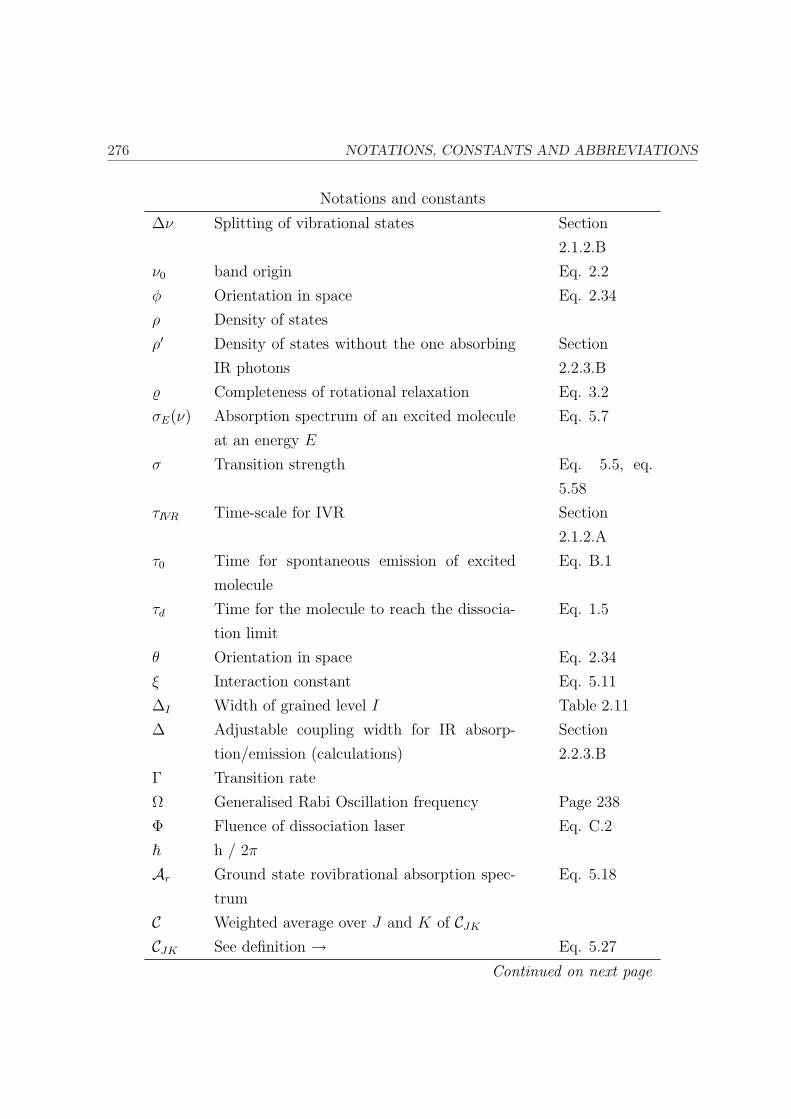
276 NOTATIONS, CONSTANTS AND ABBREVIATIONS
Notations and constants
∆ν Splitting of vibrational states Section
2.1.2.B
ν0 band origin Eq. 2.2
φ Orientation in space Eq. 2.34
ρ Density of states
ρ′ Density of states without the one absorbing
IR photons
Section
2.2.3.B
% Completeness of rotational relaxation Eq. 3.2
σE(ν) Absorption spectrum of an excited molecule
at an energy E
Eq. 5.7
σ Transition strength Eq. 5.5, eq.
5.58
τIVR Time-scale for IVR Section
2.1.2.A
τ0 Time for spontaneous emission of excited
molecule
Eq. B.1
τd Time for the molecule to reach the dissocia-
tion limit
Eq. 1.5
θ Orientation in space Eq. 2.34
ξ Interaction constant Eq. 5.11
∆I Width of grained level I Table 2.11
∆ Adjustable coupling width for IR absorp-
tion/emission (calculations)
Section
2.2.3.B
Γ Transition rate
Ω Generalised Rabi Oscillation frequency Page 238
Φ Fluence of dissociation laser Eq. C.2
~ h / 2π
Ar Ground state rovibrational absorption spec-
trum
Eq. 5.18
C Weighted average over J and K of CJK
CJK See definition → Eq. 5.27
Continued on next page
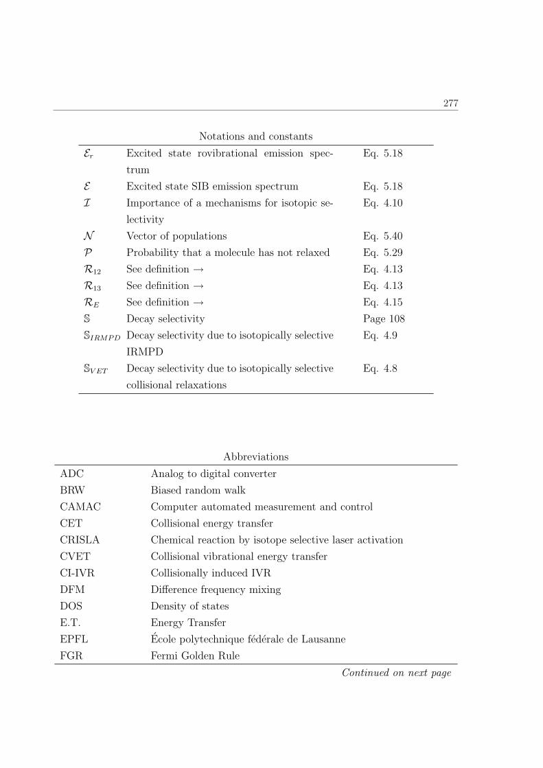
277
Notations and constants
Er Excited state rovibrational emission spec-
trum
Eq. 5.18
E Excited state SIB emission spectrum Eq. 5.18
I Importance of a mechanisms for isotopic se-
lectivity
Eq. 4.10
N Vector of populations Eq. 5.40
P Probability that a molecule has not relaxed Eq. 5.29
R12 See definition → Eq. 4.13
R13 See definition → Eq. 4.13
RE See definition → Eq. 4.15
S Decay selectivity Page 108
SIRMPD Decay selectivity due to isotopically selective
IRMPD
Eq. 4.9
SV ET Decay selectivity due to isotopically selective
collisional relaxations
Eq. 4.8
Abbreviations
ADC Analog to digital converter
BRW Biased random walk
CAMAC Computer automated measurement and control
CET Collisional energy transfer
CRISLA Chemical reaction by isotope selective laser activation
CVET Collisional vibrational energy transfer
CI-IVR Collisionally induced IVR
DFM Difference frequency mixing
DOS Density of states
E.T. Energy Transfer
EPFL Ecole polytechnique federale de Lausanne
FGR Fermi Golden Rule
Continued on next page

278 NOTATIONS, CONSTANTS AND ABBREVIATIONS
Abbreviations
FTIR Fourier Transform Infrared Spectroscopy
IC Internal conversion
IP Ionisation potential
IRF Infrared Fluorescence
IRLAPS Infrared laser assisted photofragment spectroscopy
IRMPA Infrared multiple photon absorption
IRMPE Infrared multiple photon excitation
IRMPD Infrared multiple photon dissociation
IVR Intramolecular vibrational energy redistribution
KCSI Kinetically controlled Selective Ionisation
LCPM Laboratoire de chimie physique moleculaire
LIF Laser induced fluorescence
LIS Laser isotope separation
MLIS Molecular laser isotope separation
MPA Multiple photon absorption
MPD Multiple photon dissociation
OPA Optical parametric amplification
OP-IRMPD Overtone Pre-excitation - Infrared Multiple Photon Dissociation
PA Photo-acoustic
PAL Pulsed alexandrite laser
P-E Pre-excitation
PES Potential energy surface
PMT Photo multiplier tube
PST Phase space theory
QMS Quadrupole mass spectrometer
RRK Rice-Ramsperger-Kassel
RRKM RRK-Marcus
RS Raman shifter
RS Raman scattering
SACM Statistical adiabatic channel model
SHG Second harmonic generation
Continued on next page
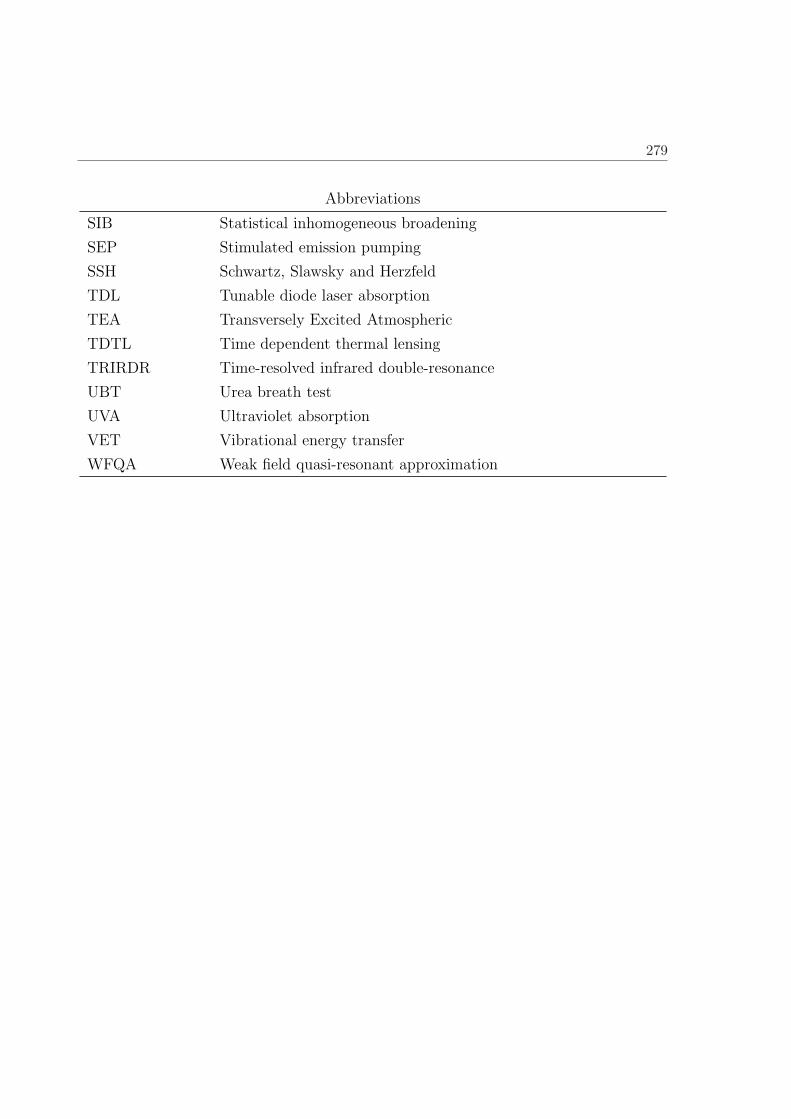
279
Abbreviations
SIB Statistical inhomogeneous broadening
SEP Stimulated emission pumping
SSH Schwartz, Slawsky and Herzfeld
TDL Tunable diode laser absorption
TEA Transversely Excited Atmospheric
TDTL Time dependent thermal lensing
TRIRDR Time-resolved infrared double-resonance
UBT Urea breath test
UVA Ultraviolet absorption
VET Vibrational energy transfer
WFQA Weak field quasi-resonant approximation

280 LIST OF TABLES
List of Tables
2.1 Normal modes and symmetry in 12CF3H and 13CF3H. . . . . . . . . . . . 20
2.2 Transition dipole moment between the ground state and the fundamentals. 21
2.3 Anharmonic constants for CF3H. . . . . . . . . . . . . . . . . . . . . . . 24
2.4 Constants for the CH chromophore in CF3H. . . . . . . . . . . . . . . . . 28
2.5 Band origins of the members of the polyads created by |Nν1〉, | (N −1)ν1 + 2ν4〉, . . . | 2Nν4〉. . . . . . . . . . . . . . . . . . . . . . . . . . . . . 29
2.6 Values of ciN,J . . . . . . . . . . . . . . . . . . . . . . . . . . . . . . . . . . 30
2.7 Integrated band strengths G. . . . . . . . . . . . . . . . . . . . . . . . . . 31
2.8 αi · 103 for B and C for CF3H. . . . . . . . . . . . . . . . . . . . . . . . . 33
2.9 Tiers of states in CF3H . . . . . . . . . . . . . . . . . . . . . . . . . . . . 37
2.10 “Slow” IVR in CF3H. . . . . . . . . . . . . . . . . . . . . . . . . . . . . . 39
2.11 Notation used for the statistical treatment. . . . . . . . . . . . . . . . . . 46
2.12 Pumping rates for the different cases A-D. . . . . . . . . . . . . . . . . . 47
2.13 Three approaches how to deal with the problem of the divergence of
P (r0, v). . . . . . . . . . . . . . . . . . . . . . . . . . . . . . . . . . . . . 59
2.14 Dependence of σ on the relative velocity of the two molecules and of
〈〈P 〉〉 on the temperature T , for the different models. . . . . . . . . . . . 59
4.1 Four schemes for the investigation of the mechanisms of the enhancement
of isotopic selectivity varying different parameters. . . . . . . . . . . . . . 107
4.2 Decay rates for molecules excited via the 52 vibrational mode with molecules
excited via another (unidentified) band . . . . . . . . . . . . . . . . . . . 113
4.3 Relative contributions of isotopically selective collisional relaxation and
isotopically selective IRMPD to the enhancement of isotopic selectivity. . 131
4.4 Experimentally measured ratio of relaxation rates. . . . . . . . . . . . . . 143
281
282 LIST OF TABLES
4.5 Results obtained for the separation of IRMPD and vibrational relaxation
for a dissociation laser frequency of 1047 cm−1 and fluence of 3 J cm−2. . 149
5.1 Shifts, widths and intensity of the SIB spectra. . . . . . . . . . . . . . . . 161
5.2 Energy and vibrational frequencies at the transition state for the lowest
dissociation channel CF3H→ CF2 + HF . . . . . . . . . . . . . . . . . . 194
6.1 Summary of relative relaxation rates of excited CF3H on ground state
CF3H. . . . . . . . . . . . . . . . . . . . . . . . . . . . . . . . . . . . . . 230
List of Figures
1.1 IRLAPS detection scheme. . . . . . . . . . . . . . . . . . . . . . . . . . . 5
1.2 Spectrum of the 31 transition in CF3H. . . . . . . . . . . . . . . . . . . . 7
1.3 Observed effect we study in this thesis. . . . . . . . . . . . . . . . . . . . 8
1.4 Collisions between the lasers and during IRMPD lower the vibrational
energy of the molecules . . . . . . . . . . . . . . . . . . . . . . . . . . . . 9
2.1 Normal modes in CF3H (frequencies for 12CF3H). . . . . . . . . . . . . . 21
2.2 FTIR scan of CF3H at room temperature. . . . . . . . . . . . . . . . . . 22
2.3 Anharmonic coupling between dark and bright states. . . . . . . . . . . . 26
2.4 Integrated absorption strengths of 0 → νCH = N . . . . . . . . . . . . . . 32
2.5 IVR . . . . . . . . . . . . . . . . . . . . . . . . . . . . . . . . . . . . . . 34
2.6 Multiple time-scales showing up in an absorption spectrum. . . . . . . . 38
2.7 Calculated redistribution of vibrational energy in a CF3H molecule ini-
tially in the v1 = 3 state. . . . . . . . . . . . . . . . . . . . . . . . . . . . 40
2.8 The two qualitatively distinct regions in IRMPD. . . . . . . . . . . . . . 42
2.9 Basic idea of the statistical treatment. . . . . . . . . . . . . . . . . . . . 45
2.10 Behaviour of up- and down-pumping rates between different bins. . . . . 51
2.11 Model for hard collisions. . . . . . . . . . . . . . . . . . . . . . . . . . . . 55
2.12 Experimental data demonstrating the dependency of the probability of
energy transfer between an excited CO2 molecule and an N2 molecule in
the ground state under the effects of long-range and short-range interac-
tion forces. . . . . . . . . . . . . . . . . . . . . . . . . . . . . . . . . . . . 62
2.13 Average energy transferred 〈∆E〉 in a collision of excited azulene at an
energy E, for different bath gas molecules. . . . . . . . . . . . . . . . . . 65
283

284 LIST OF FIGURES
2.14 Example of the dependence of the vibrational relaxation rate on the vi-
brational excitation, for the case of excited O2 relaxing on N2. . . . . . . 68
2.15 Temperature dependency for CO(0001)+CO(0000)→ CO(0000)+CO(0001)
and for CO(0001)+N2(v=0) → CO(0000)+N2(v=1) collisions. . . . . . . 70
2.16 Average energy 〈〈∆E〉〉 transferred between an excited molecule and the
same unexcited species. . . . . . . . . . . . . . . . . . . . . . . . . . . . . 72
3.1 General energy level diagram used in our experiments. . . . . . . . . . . 88
3.2 Optical setup of the experiments. . . . . . . . . . . . . . . . . . . . . . . 90
3.3 Timing of pre-excitation, dissociation and LIF lasers. . . . . . . . . . . . 93
3.4 Generation of the laser beam for pre-excitation of CF3H molecules via
the 21 band. . . . . . . . . . . . . . . . . . . . . . . . . . . . . . . . . . . 94
3.5 Generation of the laser beam for pre-excitation of CF3H molecules via
the 21 band. . . . . . . . . . . . . . . . . . . . . . . . . . . . . . . . . . . 95
3.6 The decay rate k goes up as p goes down, indicating that molecules flying
out of the reaction volume falsify the experimental measurement. . . . . 97
3.7 Measurements for rotational relaxation. . . . . . . . . . . . . . . . . . . . 98
3.8 Completeness of rotational relaxation. . . . . . . . . . . . . . . . . . . . . 99
3.9 Initial setup for the production of 13C enriched CF3H. . . . . . . . . . . . 100
3.10 Procedure for the synthesis of 13CF3H. . . . . . . . . . . . . . . . . . . . 101
3.11 Comparison of measured and literature mass-spectra for the identification
of the gas. . . . . . . . . . . . . . . . . . . . . . . . . . . . . . . . . . . . 102
3.12 Mass spectrum of the final products of the 13CF3H synthesis. . . . . . . . 103
4.1 General experimental procedure. . . . . . . . . . . . . . . . . . . . . . . . 106
4.2 Successive measurements of the decay rate k. . . . . . . . . . . . . . . . . 109
4.3 Energy scheme used in the experiments for the determination state speci-
ficity of relaxation rates. . . . . . . . . . . . . . . . . . . . . . . . . . . . 111
4.4 Experiments to test the influence of the rotational identity of the pre-
excited state on the decay rates. . . . . . . . . . . . . . . . . . . . . . . . 112
4.5 Experiments to test the influence of the vibrational identity of the pre-
excited state on the decay rates. . . . . . . . . . . . . . . . . . . . . . . . 113
4.6 Energy scheme used in the experiments for the determination of photofrag-
ment excitation spectra of excited molecules. . . . . . . . . . . . . . . . . 115

285
4.7 Sample curves of measured dissociation yields. . . . . . . . . . . . . . . . 116
4.8 Sample curves of measured dissociation probability. . . . . . . . . . . . . 117
4.9 ν0, ω and B found for the photofragment spectra of excited 12CF3H and13CF3H for different fluences of the CO2 laser. . . . . . . . . . . . . . . . 118
4.10 An IRLAPS action spectrum around the Q-branch of the 31 band in13CF3H is split into two parts due to the two different isotopomers. . . . 120
4.11 Example of a measurement of the dissociation selectivity SIRMPD. . . . . 121
4.12 Dissociation selectivity SIRMPD for 3 J cm−2 and for 9 J cm−2. . . . . . . 122
4.13 Dissociation selectivity SIRMPD for molecules pre-excited via the 31 and
via the 21 bands for a dissociation laser frequency of 1047 cm−1. . . . . . 123
4.14 Comparison of experimental and predicted dissociation yields. . . . . . . 125
4.15 Energy scheme used in the experiments for the relaxation experiments
changing the wavelength of the dissociation laser. . . . . . . . . . . . . . 128
4.16 Sample measurements of the decay rate k. . . . . . . . . . . . . . . . . . 129
4.17 Decay rate k for 12CF3H and 13CF3H at a fluence of Φ = 3 J cm−2 as a
function of the dissociation laser frequency. . . . . . . . . . . . . . . . . . 130
4.18 SIRMPD and SV ET determined by changing the wavelength of the CO2
dissociation laser. . . . . . . . . . . . . . . . . . . . . . . . . . . . . . . . 131
4.19 Importance I of a mechanism for the enhancement of isotopic selectivity
upon leaving a time-delay between the pre-excitation and the dissociation
lasers. . . . . . . . . . . . . . . . . . . . . . . . . . . . . . . . . . . . . . 132
4.20 Energy scheme used in the experiments for the relaxation experiments
using 13CF3H as relaxation partner of excited CF3H. . . . . . . . . . . . 135
4.21 Example of measurement of the decay rate k for different isotopic com-
position of the sample for 12CF3H and 13CF3H. . . . . . . . . . . . . . . 136
4.22 Values for k(x? − y) for molecules pre-excited via the 31 band. . . . . . . 137
4.23 Values for k(x? − y) for molecules pre-excited via the 21 , 41 and 52 bands.138
4.24 Schematic absorption and emission spectra of 12CF3H and 13CF3H for
molecules in the ground state and with 8800 cm−1 vibrational energy. . . 140
4.25 Values for R12 and R13 for different pre-excitation energies and dissoci-
ation laser conditions. . . . . . . . . . . . . . . . . . . . . . . . . . . . . 142
4.26 Relative relaxation rates R12 and R13. . . . . . . . . . . . . . . . . . . . 144
4.27 Interpretation of our results obtained with isotopically enriched samples. 145

286 LIST OF FIGURES
4.28 Measured values of SIRMPD. . . . . . . . . . . . . . . . . . . . . . . . . . 146
4.29 Contributions of isotopically selective collisional relaxation and different
IRMPD efficiencies to the increase of isotopic selectivity, for different
pre-excitation levels and fluences. . . . . . . . . . . . . . . . . . . . . . . 147
4.30 Experimentally determined ratio of relaxation rates. . . . . . . . . . . . . 150
5.1 Absorption spectra for CF3H molecules at 0, 2500, 5000, 7500, . . ., 20,000
cm−1. . . . . . . . . . . . . . . . . . . . . . . . . . . . . . . . . . . . . . 158
5.2 SIB absorption spectra for ν2, ν3 and ν6. . . . . . . . . . . . . . . . . . . 159
5.3 The transition spectra of excited molecules shift, broaden and get more
intense as the energy of the molecules increase. . . . . . . . . . . . . . . . 160
5.4 For the calculation of the whole absorption spectrum the SIB spectrum
is convoluted with a rotational contour. . . . . . . . . . . . . . . . . . . . 164
5.5 The calculation of the transition rate is done by integrating over the
trajectory. . . . . . . . . . . . . . . . . . . . . . . . . . . . . . . . . . . . 171
5.6 Absolute vibrational energy transfer rates for V-V relaxation mediated
by the ν5 mode. . . . . . . . . . . . . . . . . . . . . . . . . . . . . . . . . 174
5.7 Relaxation rates associated with a particular mode. . . . . . . . . . . . . 175
5.8 The shift between absorption and emission spectra as a function of the
energy of the donor molecule. . . . . . . . . . . . . . . . . . . . . . . . . 176
5.9 Parts (I) and (II) of equation 5.37 and the total relaxation rate (relative
values). . . . . . . . . . . . . . . . . . . . . . . . . . . . . . . . . . . . . 177
5.10 Contribution of ν5 to the V-V energy transfer process. . . . . . . . . . . . 180
5.11 Results for R12 and R13 where only vibrational energy transfer via long
range dipole-dipole interactions are considered. . . . . . . . . . . . . . . . 180
5.12 Pairs of R0 and ℵ′ which fit to the measured isotopic selectivity of the
relaxation rates well. . . . . . . . . . . . . . . . . . . . . . . . . . . . . . 184
5.13 Calculated and experimental relative relaxation rates of vibrationally ex-
cited CF3H on 12CF3H in the vibrational ground state. . . . . . . . . . . 185
5.14 Relaxation rates as a function of the energy in the molecule (for R0 =
7.4 A, ℵ′ = 6.8 · 104 cm−1). . . . . . . . . . . . . . . . . . . . . . . . . . . 186
5.15 Energy level diagram for master equation calculations. . . . . . . . . . . 189
287
5.16 Arrhenius plots of experimental data for CF3H measured by different
authors. . . . . . . . . . . . . . . . . . . . . . . . . . . . . . . . . . . . . 195
5.17 Absorption spectrum for calculations based on a statistical treatment. . . 198
5.18 Example of a simulated three laser experiment. . . . . . . . . . . . . . . 201
5.19 Energy distributions for the example shown in figure 5.18. . . . . . . . . 202
5.20 Dynamics of energy level populations calculated for 12CF3H and for 13CF3H.203
5.21 Simulated and measured dissociation yields. . . . . . . . . . . . . . . . . 205
5.22 Absorption spectrum of two quanta in the ν6 vibration for molecules with
a vibrational energy of 8800 cm−1. . . . . . . . . . . . . . . . . . . . . . . 206
5.23 Dissociation yield of molecules pre-excited via the 31 band, with a disso-
ciation laser frequency of 977 cm−1. . . . . . . . . . . . . . . . . . . . . . 207
5.24 Photofragment spectra of vibrationally excited 12CF3H for off-resonant
dissociation laser frequencies. . . . . . . . . . . . . . . . . . . . . . . . . 208
5.25 Measured and calculated centres ν0 of the photofragment spectra of vi-
brationally excited 12CF3H. . . . . . . . . . . . . . . . . . . . . . . . . . 209
5.26 Simulated and measured dissociation selectivities for a sample at 0.4 mbar.210
5.27 Laser pulses used for the experiments elsewhere. . . . . . . . . . . . . . . 212
5.28 Overall selectivity of the dissociation yields as a function of the pressure
of the sample. . . . . . . . . . . . . . . . . . . . . . . . . . . . . . . . . . 213
5.29 Measured and calculated decay rates for 12CF3H and 13CF3H. . . . . . . 213
5.30 Numerical evaluation of the contributions of the different mechanisms to
the increase of isotopic selectivity, for a frequency of the dissociation laser
of 1047 cm−1. . . . . . . . . . . . . . . . . . . . . . . . . . . . . . . . . . 215
5.31 Simulated dissociation probability for 12CF3H and 13CF3H molecules. . . 217
5.32 Calculated dissociation probabilities. . . . . . . . . . . . . . . . . . . . . 218
5.33 Dissociation selectivity and yield for pre-excitation via the 31 and the 41
bands. . . . . . . . . . . . . . . . . . . . . . . . . . . . . . . . . . . . . . 219
5.34 Dissociation selectivity and yield for a dissociation laser fluence of 1, 3
and 5 J cm−2. . . . . . . . . . . . . . . . . . . . . . . . . . . . . . . . . . 219
5.35 Dissociation selectivity and yield for a dissociation laser frequency of
1039, 1044 and 1049 cm−1. . . . . . . . . . . . . . . . . . . . . . . . . . . 220
288 LIST OF FIGURES
A.1 In case C, the states in both the upper and lower bins are uncoupled
amongst each other. . . . . . . . . . . . . . . . . . . . . . . . . . . . . . . 236
A.2 Rabi-oscillations for different strengths of coupling between the two states.237
A.3 D is the off-resonance shift between the difference of energy of the two
levels and the frequency of the electromagnetic field. . . . . . . . . . . . . 238
A.4 Evolution of upper level J . . . . . . . . . . . . . . . . . . . . . . . . . . . 241
B.1 Sample LIF signal. . . . . . . . . . . . . . . . . . . . . . . . . . . . . . . 244
B.2 Quenching of CF2 on CF3H. . . . . . . . . . . . . . . . . . . . . . . . . . 245
B.3 Correction factors ε for the dissociation yield. . . . . . . . . . . . . . . . 245
C.1 Absorption spectrum of teflon. . . . . . . . . . . . . . . . . . . . . . . . . 248
C.2 Amount of transmitted light f1 by the Pellin-Broca prism and the BaF2
windows of the cell. . . . . . . . . . . . . . . . . . . . . . . . . . . . . . . 249
C.3 Measurements of f2, the amount of the CO2 laser shot used. . . . . . . . 250
C.4 By scanning a slit over the beam we measure a Gaussian dependence of
the energy let through as a function of the displacment. . . . . . . . . . . 250
C.5 Cross-section of the CO2 laser beam at the focal point and output energy
of pulse. . . . . . . . . . . . . . . . . . . . . . . . . . . . . . . . . . . . . 251
D.1 Example of a measurement of k as a function of the fluence of the disso-
ciation laser. . . . . . . . . . . . . . . . . . . . . . . . . . . . . . . . . . . 254
D.2 Illustration of why k goes through a maximum as a function of the fluence
of the dissociation laser. . . . . . . . . . . . . . . . . . . . . . . . . . . . 255
E.1 Principle of our code . . . . . . . . . . . . . . . . . . . . . . . . . . . . . 258

Acknowledgements
This thesis would not have been possible without the help of many people.
First of all, I would like to thank my thesis advisor Prof. Tom Rizzo for his confidence
in me and in giving me the opportunity to perform the research under his direction.
His guidance and motivation were always of great help.
My deep gratitude and appreciation goes to Dr. Oleg Boyarkin, my supervisor, for
guiding me through the wonder- and colourful world of laser spectroscopy and for his
continuous support during all these years.
A special thank you goes to Dr. Mikhail Polianski with whom I shared the lab and
with whom I spent hours in front of the black board developing models on laser isotope
separation and vibrational energy transfer. Thanks also for the great help in every day
problems in the lab (e.g. fixing lasers I broke before).
I wish to thank my colleagues Plinio Maroni and Thanh Tung Dang, with whom Misha
and I shared the office during several years. A great thank you to all of you guys for the
lovely time we spent together, for your humour, your joy and the coffee breaks ! Thank
you for supporting me in moments of fluctuating mood (especially when I was writing
up the thesis !).
Thanks are due to present and former LCPM members: Dr. Rainer Beck, Dr. Andreas
Braun, Dr. Andrea Callegari, Rachele Chianese, Dr. Marcel Drabbels, Prof. Tino
Gaumann, Monia Giudi, Anthi Kamariotis, Dr. Aziz Kasimov, Dr. Monika Kowalczyk,
Evgeniy Loginov, Dr. Joachim Makowe, Pavel Maksyutenko, Sebastien Mercier, An-
289
290 ACKNOWLEDGEMENTS
toine Milon, Dr. Dimitrios Papageorgopoulos, Dr. Julia Rebstein, Dr. David Rueda,
Marco Sacchi, Dr. Mathieu Schmid, Dr. Patrice Theule.
A special thanks goes to Amanz Ruf who helped me with the synthesis of 13CF3H
(poor guy having to teach chemistry to a physicist !) and a very special thanks goes to
Marianne Dang whose support went well beyond administrative matters.
I am grateful to all my physicist- and mathematician-friends: Celine, Yvonne, Chris-
tian, Dominique (“Gruessech !”), Fabien (who does not appreciate jam together with
Gruyeres cheese on bread), Gilles (moi je pense pas que t’es de mauvaise foi), Loic (my
“coloc”), Pierre (who managed to finish his thesis before me.... grrr !), Raphael and
Reda (if you want to know where the best strawberries come from... he knows !). A
particular thanks to Severine for her continuous support, her joy and her advice. And
for equation (3.13).
A very special thanks goes to my very special friends Myriam and Daniel, for all the
great time we spent together and for all their support during darker moments of my life.
I am forever indebted to my parents for their support and encouragement when it was
most required. Without their support, I would not be where I am now. An enormous
hug and thanks goes to my most beloved sister Olivia, for her humour and her support.
Thank you also for the time trying to explain chemistry to your “brudder”.
Last, but not least, I wish to tenderly thank Valerie for having shared the past couple of
years with me, for all her love, her understanding and patience also in difficult moments.

Curriculum vitae: Richard Bossart
Rue St-Roch 5
1004 Lausanne
Switzerland
Birthdate and -place: 25 December 1974, Win-
terthur
Swiss and British Citizenship.
Maritial status: Single
2005 Research&Development at Rolex, Geneva
2000-05 PhD thesis in physical chemistry, EPFL, Switzerland
supervised by Prof. Tom Rizzo
“On Isotopically Selective Collisional Energy Transfer and
Infrared Multiple Photon Absorption by Vibrationally Highly
Excited Molecules”
2000 Masters thesis in cluster physics, EPFL, Switzerland
supervised by Prof. Christian Felix
“Development of a source of silver clusters with the pick-up
method”
1997/98 Year at Imperial College, London
1995-2000 Studies in physics at EPFL, Switzerland
1995 Maturtatszeugnis Realgymnasium Bern-Kirchenfeld, Switzerland
291