On Goodput and Energy Measurements of Network Coding ... · electronics Article On Goodput and...

Aalborg Universitet

On Goodput and Energy Measurements of Network Coding Schemes in the RaspberryPi

Hernandez, Nestor; Sørensen, Chres Wiant; Cabrera, Juan; Wunderlich, Simon ; Roetter,Daniel Enrique Lucani; Fitzek, FrankPublished in:Eletronics

DOI (link to publication from Publisher):10.3390/electronics5040066

Creative Commons LicenseCC BY 4.0

Publication date:2016

Document VersionPublisher's PDF, also known as Version of record

Link to publication from Aalborg University

Citation for published version (APA):Hernandez, N., Sørensen, C. W., Cabrera, J., Wunderlich, S., Roetter, D. E. L., & Fitzek, F. (2016). On Goodputand Energy Measurements of Network Coding Schemes in the Raspberry Pi. Eletronics, 5(4).https://doi.org/10.3390/electronics5040066

General rightsCopyright and moral rights for the publications made accessible in the public portal are retained by the authors and/or other copyright ownersand it is a condition of accessing publications that users recognise and abide by the legal requirements associated with these rights.

? Users may download and print one copy of any publication from the public portal for the purpose of private study or research. ? You may not further distribute the material or use it for any profit-making activity or commercial gain ? You may freely distribute the URL identifying the publication in the public portal ?

Take down policyIf you believe that this document breaches copyright please contact us at [email protected] providing details, and we will remove access tothe work immediately and investigate your claim.

https://doi.org/10.3390/electronics5040066

https://vbn.aau.dk/en/publications/ed3fb049-16f7-4f87-bd89-8c1884d34fad

https://doi.org/10.3390/electronics5040066

electronics

Article

On Goodput and Energy Measurements ofNetwork Coding Schemes in the Raspberry Pi

Néstor J. Hernández Marcano 1,2,*,†, Chres W. Sørensen 2,†, Juan A. Cabrera G. 3,4,Simon Wunderlich 3, Daniel E. Lucani 2,† and Frank H. P. Fitzek 3

1 Steinwurf ApS, Aalborg Øst 9220, Denmark2 Department of Electronic Systems, Aalborg University, Aalborg Øst 9220, Denmark;

[email protected] (C.W.S.); [email protected] (D.E.L.)3 Deutsche Telekom Chair of Communication Networks, Technische Universität Dresden, Dresden 01062,

Germany; [email protected] (J.A.C.G.); [email protected] (S.W.);[email protected] (F.H.P.F.)

4 SFB 912—Collaborative Research Center HAEC, Dresden 01062, Germany* Correspondence: [email protected] or [email protected]; Tel.: +45-51-20-03-49† Current address: Fredrik Bajers Vej 7A, Room A3-110, Aalborg Øst 9220, Denmark.

Academic Editor: Mostafa BassiouniReceived: 30 June 2016; Accepted: 29 August 2016; Published: 13 October 2016

Abstract: Given that next generation networks are expected to be populated by a large number ofdevices, there is a need for quick deployment and evaluation of alternative mechanisms to cope withthe possible generated traffic in large-scale distributed data networks. In this sense, the Raspberry Pihas been a popular network node choice due to its reduced size, processing capabilities, low cost andits support by widely-used operating systems. For information transport, network coding is a newparadigm for fast and reliable data processing in networking and storage systems, which overcomesvarious limitations of state-of-the-art routing techniques. Therefore, in this work, we provide anin-depth performance evaluation of Random Linear Network Coding (RLNC)-based schemes forthe Raspberry Pi Models 1 and 2, by showing the processing speed of the encoding and decodingoperations and the corresponding energy consumption. Our results show that, in several scenarios,processing speeds of more than 80 Mbps in the Raspberry Pi Model 1 and 800 Mbps in the RaspberryPi Model 2 are attainable. Moreover, we show that the processing energy per bit for network codingis below 1 nJ or even an order of magnitude less in these scenarios.

Keywords: network coding; Raspberry Pi; goodput; energy; performance

1. Introduction

Due to the advent of the Internet of Things (IoT), approximately 50 billion devices rangingfrom sensors to phones are expected to be connected through data networks in a relatively shortperiod of time [1]. This massive deployment requires the design and testing of new distributedsystems that permit one to manage the amount of traffic from the proposed services provided bythese devices. Therefore, development platforms that help to quickly deploy, analyze and evaluatethis type of scenario are highly desirable for research. With the emergence of the Raspberry Pi (Raspi),a lrelatively powerful low-cost computer with the size of a credit card, these evaluations are becomingpossible now. This platform has been used as general purpose hardware for IoT applications asreported in surveys, such as [2]. In these applications, the Raspi might be the sensoring or computingentity (or even both) for a required task. To achieve this, it can be extended from being a simplecomputer using self-designed or already available extension modules.

A benefit of using the Raspi as a development platform is its large community of supporters.By running standard operating systems, such as Linux or Windows, this permits one to utilize

Electronics 2016, 5, 66; doi:10.3390/electronics5040066 www.mdpi.com/journal/electronics

http://www.mdpi.com/journal/electronics

http://www.mdpi.com

http://www.mdpi.com/journal/electronics

Electronics 2016, 5, 66 2 of 27

standard, well-tested and reliable tools to administrate and maintain these networks in a flexible,stable and supported manner, which is a major requirement to make a scalable deployment. Moreover,by enabling system designers to configure and deploy several devices at the same time, possibledeployments of tens, hundreds or even thousands of Raspberry Pi’s would allow one to analyzerepresentative data patterns of the IoT. Different use cases of IoT applications employing the Raspias a building block can be found in the literature. A basic study of the Raspi as a possible device forsensor applications can be found in [3]. The authors in [4] consider using the Raspi as an IPv6 overLow power Wireless Personal Area Networks (6LoWPAN) gateway for a set of sensor and mobiledevices to an Internet Protocol (IP) Version 6 network. In [5], a general purpose sensoring platformfor IoT is presented using the Raspi as its basic building block. Various interesting IoT use cases arethe works presented in [6–9]. In [6], many Raspis are used as controllable smart devices with networkconnectivity that may ubiquitously interact with different users, each represented by a mobile devicethrough a smartphone application. The study in [7] considers Raspis as a data processing unit fordisseminating artwork content in smart museums. An IoT setting where the Raspi is employed asa nano-server in distributed storage and computing can be found in [8]. Finally, in [9], the authorspresent the Raspi as the processing entity of an unmanned areal vehicle application to increase theresilience of wireless sensor networks. However, despite all of these advances in the IoT area regardingthe exploitation of the Raspi capabilities, the application data are forwarded using former conventionalrouting methods, which may not satisfy the need of a distributed network for IoT applications asmentioned earlier.

In this context, introduced in [10], Network Coding (NC) constitutes a paradigm shift in the waydata networks are understood by changing how information is sent through them and stored at theend devices. Instead of treating the packets as atomic unmodifiable units, packets are seen as algebraicentities in a Galois Field (GF) that can be operated on to create new coded packets. This permits one toremove the limitation of sending specific packets by now sending coded packets as linear equations ofthe original ones. This change in the way of seeing how the data are represented brings new featuresthat can be exploited. In this way, instead of typically encoding and decoding on a hop basis, relayingnodes can take part in the coding process without needing to decode. Therefore, a relay can recodepackets, i.e., encode again previously-received encoded (but not decoded) packets in order to reducedelay and still take advantage of the data representation for the next hop. This new type of codingacross the network is proven to achieve the multicast capacity [10,11].

Compared to other broadly-used coding schemes, such as Low Density Parity Check (LDPC)codes [12] or Reed–Solomon codes [13], network coding is a technology that has been studied andimplemented in real systems since the early years of its conception. A decentralized network codethat has been proven to achieve the multicast capacity with very high probability is RLNC [14].Later, a work observing the benefits of employing RLNC in meshed networks is the Multi-pathOpportunistic Routing Engine (MORE) protocol addressed in [15]. Shortly afterwards, the authorsin [16] showed the performance of an implementation of the COPE protocol for the two-way relaychannel in a wireless network, which relied on minimalistic coding and obtaining gains over aforwarding scheme. Later, the work in [17] used commercially-available Symbian OS mobile phones toimplement network coding in a Device to Device (D2D) cooperation-based application. Furthermore,in [18], the Kodo library was introduced. Kodo is a C++11 network coding library intended to makenetwork coding basic functionalities easily available for both the research community and commercialentities. Based on Kodo, the Coding Applied To Wireless On Mobile Ad-hoc Networks (CATWOMAN)protocol [19] is implemented on top of the Better Approach To Mobile Ad-hoc Networking (BATMAN)protocol [20] for WiFi multi-hop meshed networks. It uses some of the intuition from COPE, butit is deployed within the X topology with overhearing links. Its source code is available as opensource in the Linux kernel. Moreover, many other successful implementations have been tested onreal-world systems, such as found in [21–24]. For the Raspberry Pi device, an evaluation of RLNCcan be found in [25]. However, this evaluation focused particularly on observing the achievable


speeds only for RLNC with different configurations of the code parameters. In this previous work,a relevant practical aspect that was not evaluated was the use of hardware acceleration throughSingle Instruction Multiple Data (SIMD) or the multi-core capabilities of more advanced Raspimodels. These features are becoming more frequent in new processors to largely increase theircomputational power for the upcoming demand. In this sense, the Raspberry Pi posses an AdvancedRISC Machine (ARM) architecture that could be multi-core, as mentioned, and also exploits the SIMDfeature with the optimized NEON instruction set, but still to the best of our knowledge, there has beenno documentation in the literature about these capabilities.

Therefore, in this work, we provide detailed measurements of the goodput (processing speed)and energy consumption of Raspi Models 1 and 2, when performing network coding operations withdifferent codecs based on RLNC such as: full dense RLNC, multi-core enabled RLNC, sparse RLNCand tunable sparse RLNC. For these coding schemes, the encoder and decoder implementationsfrom Kodo are able to detect and make use of the SIMD through the NEON instruction set of theRaspberry Pi by recognizing the ARM architecture with its multicore capabilities. We assess theRaspi performance excluding the effect of packet losses or delays in order to have a description of theprocessing and energy consumption for only the codes in terms of their parameters. To achieve this, weperform a measurement campaign with the indicated coding schemes and their parameters in variousmodels of a Raspberry Pi device. Our measurements permit us to characterize the mentioned metricsof these devices showing that processing speeds of 800 Mbps and processing energy per bit values of0.1 nJ are possible. Our work is organized as follows. Section 2 defines the coding schemes employed inour study. Later, in Section 3, we describe the considered metrics and methodology for the performancecomparison of the codes deployed in the Raspi. In Section 4, we show the measurements in the Raspimodels of the mentioned metrics providing full discussions about the observed operational regimesand effects. Final conclusions and future work are reviewed in Section 5.

2. Coding Schemes

In this section, we present the considered coding schemes that are evaluated in the Raspi 1 and 2.We introduce a definition for the primitive coding operations, e.g., encoding, decoding and recoding(where it applies) for each coding scheme. Later, we address particular schemes, which are obtainedby modifying the basic coding operations that provide better processing speeds, which is particularlyrelevant for the Raspi. Finally, we include a review of algorithms for network coding that exploit themulticore capabilities of the Raspi 2.

2.1. Random Linear Network Coding

RLNC is an example of intra-session NC, i.e., data symbols from a single flow are combinedwith each other. In this type of network coding, g original data packets, also called a generation [26],Pj, j ∈ [1, 2, . . . , g], each of B bytes, are used to create coded packets using random linear combinationsof the original ones. In the following subsections, we describe the basic functionalities of RLNC.

2.1.1. Encoding

In RLNC, any coded packet is a linear combination of all of the original packets. For the codingscheme, packets are seen as algebraic entities formed as a sequence of elements from GF(q), which isa GF of size q. Later, each original packet is multiplied by a coding coefficient from GF(q). The codingcoefficients are chosen uniformly at random from the GF by the encoder. To perform the multiplicationof a packet by a coding coefficient, the coefficient is multiplied for each of the elements in theconcatenation that composes an original packet, preserving the concatenation. Later, all resultingpackets are added within the GF arithmetics together to generate a coded packet. Thus, a coded packetcan be written as:


Ci =g⊕

j= 1

vij ⊗ Pj, ∀i ∈ [1, 2, . . .) (1)

In (1), Ci is the generic coded packet. In principle, the encoder may produce any numberof coded packets, but a finite number is produced in practice given that a decoder needs only glinearly-independent coded packets to decode the batch. Furthermore, in (1), vij is the coding coefficientused in the i-th coded packet and assigned to multiply the j-th original packet.

For indicating to a receiver how the packets were combined to create a coded one, a simple, yetversatile choice is to append its coding coefficients as a header in the coded packet. Hence, an amountof overhead is included in every coded packet given that we need to provide some signaling neededfor decoding. The coding coefficients overhead amount for packet i, |vi|, can be quantified as:

|vi| =g

∑j= 1|vij| = g× dlog2(q)e [bits]. (2)

2.1.2. Decoding

To be able to decode a batch of g packets, a linearly-independent set of g coded packets, Ci,i ∈ [1, 2, . . . , g], is required at a decoder. Once this set has been collected for a decoder, the originalpackets can be found by computing the solution of a system of linear equations using GF arithmetics.Thus, we define C =

[C1 . . . Cg

]T , P =[P1 . . . Pg

]T and the coding matrix V that collects the codingcoefficients for each of the g coded packets, as follows:

V =

v1...

vg

=

v11 . . . v1g...

. . ....

vg1 . . . vgg

. (3)

Algebraically, decoding simplifies to finding the inverse of V in the linear system C = VP, whichcan be achieved using efficient Gaussian elimination techniques [27]. On real applications, decoding isperformed on-the-fly, e.g., the pivots are computed as packets are progressively received, in order tominimize the computation delay for each step.

A decoder starts to calculate and subtract contributions from each of the pivot elements, e.g.,leftmost elements in the main diagonal of (3), from top to bottom. The purpose is to obtain theequivalence V in its reduced echelon form. The steps for reducing the matrix by elementary rowoperations are carried out each time a linearly-independent packet is received. Once in reducedechelon form, packets can be retrieved by doing a substitution starting from the latest coded packet.In this way, the amount of elementary operations at the end of the decoding process is diminished.

2.1.3. Recoding

As an inherent property of RLNC, an intermediate node in the network is able to create newcoded packets without needing to decode previously-received packets from an encoding source.Therefore, RLNC is an end-to-end coding scheme that permits one to recode former coded packets atany point in the network without requiring a local decoding of the data. In principle, a recoded packetshould be indistinguishable from a coded one. Thus, we define a recoded packet as Ri and considerthe coding coefficients wi1, . . . , wig as used to create Ri. Later, a recoded packet can be written as:

Ri =g⊕

j= 1

wij ⊗ Cj, ∀i ∈ [1, . . .). (4)


In (4), wij is the coding coefficient used in the i-th recoded packet and assigned to multiplya previously-coded packet Cj. These coding coefficients are again uniformly and randomly chosenfrom GF(q). However, these wij’s are not appended to the previous coding coefficients. Instead,the system will update the previous coefficients. Due to the linearity of the operation, this updatereduces to recombining the coding coefficients equivalent to each original packet with the weight ofthe wi,j.Therefore, we define the local coding matrix W in the same way as it was made for V. Thus,the local coding matrix can be written as:

W =

w1...

wg

=

w11 . . . w1g...

. . ....

wg1 . . . wgg

. (5)

With the definitions from (3) and (5), the recoded packets R =[R1 . . . Rg

]T are written asR = (WV)P. Here, we recognize the relationship between original and recoded packets. The resultingcoding matrix is the multiplication of matrices W and V. Denoting (WV)ij as the element in the i-throw and j-th column of (WV), this term is the resulting coding coefficient used to create Ri afterencoding the original packet Pj recoding it locally in an intermediate node. Finally, the appendedcoefficients for Ri are (WV)ik with k ∈ [1, 2, . . . , g]. By doing some algebra, each (WV)ij term can beverified to be computed as:

(WV)ij =g

∑k = 1

wikvkj , ∀i, j ∈ [1, 2, . . . , g]× [1, 2, . . . , g]. (6)

This update procedure on the coding coefficients is carried by all of the recoders in a givennetwork, therefore allowing any decoder to compute the original data after Gaussian elimination,regardless of the amount of times recoding was performed and without incurring in any additionaloverhead cost for signaling. Similar to the encoding operation, any decoder that collects a set of glinearly-independent recoded packets with their respective coefficients will be able to decode the dataas mentioned before in Section 2.1.2.

2.2. Sparse Random Linear Network Coding

In Sparse Random Linear Network Coding (SRLNC), instead of considering all of the packets tocreate a coded packet as in RLNC, an encoder sets more coding coefficients to zero when generatinga coded packet with the purpose of reducing the overall processing. Decoding is the same as in RLNC,but given that the coding matrices are now sparse means that there will be less operations to performin the decoding process. Recoding, although theoretically possible, is omitted since it requires the useof heuristics to keep packets sparse after recoding, which is inherently sub-optimal. In what follows,we describe the coding scheme with two different methods to produce sparse coded packets.

2.2.1. Method 1: Fixing the Coding Density

A way to control the amount of non-zero coding coefficients is to set a fixed ratio of non-zerocoefficients in the encoding vector of size g. We refer to this fixed ratio as the average coding density d.Thus, for any coded packet Ci with coding coefficients vij, j ∈ [1, 2, . . . , g], its coding density is definedas follows:

d =∑

gj= 1 f (vij)

g, f (vij) =

{0 , vij = 0

1 , vij 6= 0(7)

From the density definition in (7), it can be observed that 0 ≤ d ≤ 1. As g increased, we obtainmore granularity in the density. Notice that the special case of d = 0 has no practical purpose, since


it implies just zero padded data. Therefore, a practical range for the density excludes the zero case,0 < d ≤ 1. Furthermore, in GF(2), there is no benefit of using d > 0.5 in terms of generatinglinearly-independent packets [28]. Thus, we limit the range to 0 < d ≤ 0.5 in GF(2).

To achieve a desired average coding density in the coefficients, for each of them, we utilize a setof Bernoulli random variables all with parameter d as its success probability, i.e., Bj ∼ Bernoulli(d),∀j ∈ [1, 2, . . . , g]. In this way, we can represent a coded packet in SRLNC as:

Ci =g⊕

j= 1

Bjvij ⊗ Pj, vij 6= 0 ∀i ∈ [1, . . .), d ∈{(0, 0.5] , q = 2

(0, 1] , q > 2(8)

In (8), we have the requirement for the coding coefficient to not be zero, since we want toensure that a coding coefficient is generated for any random trial, where Bj = 1. Therefore, in ourimplementation of SRLNC, we exclude the zero element and then pick uniformly-distributed randomelements from GF(q)−{0}. Furthermore, we have specified a dependency on the field size for practicaldensity values. In the case of employing GF(2), the maximum plausible density is restricted up to 0.5,since higher values incur in more frequent linearly-dependent coded packets [28] accompanied byhigher coding complexity.

Reducing d enables the encoder to decrease the average number of packets mixed to make a codedone. This reduces the complexity of the encoder since it needs to mix less packets. Moreover, it alsosimplifies the decoder processing given that less nonzero coding coefficients are required to be operatedduring the Gaussian elimination stage.

The drawback of this scheme is that coded packets from the encoder become more linearlydependent on each other as the density is reduced. This leads to transmission overhead since anothercoded packet is required to be sent for every reception of a redundant packet. Furthermore, thismethod may still generate a coded packet, which does not contain any information. For example,we might find the case where

[B1, . . . ,Bg

]= 0 to occur frequently for low densities. In that case,

the encoder discards the coded packet and tries to generate a new one to avoid the negative impact onoverall system performance.

2.2.2. Method 2: Sampling the Amount of Packets to Combine

The method described from (8) results in a fast implementation in terms of execution time ford ≥ 0.3 [29]. It is however not able to utilize the full performance potential for low densities, as thetotal number of Bernoulli trials remains unchanged independently of the density. Thus, we introducea second method that permits a faster implementation for low coding densities [29].

For this method, we first obtain the amount of packets that we will combine to createa coded packet. To do so, a random number, M, of the original packets is used to producea coded packet. For our case, M is binomially distributed with parameters g for the number oftrials and d for its success probability, e.g., M ∼ Binomial(g, d). However, when sampling from thisdistribution, the case M = 0 occurs with a non-zero probability. In order to handle this special case,our implementation considers K = max(1,M) as the final amount of packets to be mixed together.In this way, we always ensure that at least one packet is encoded.

The only caveat is that the case of K = 1 occurs slightly more often than M = 1 in theoriginal distribution, but for the considered density range in this method, this is not a significantmodification [29]. Then, once the distribution for the number of packets to mix has been defined, wesample a value m from M and compute k = max(1, m). Later, we create a set K with cardinality k,e.g., |K| = k, where the elements in K are the indexes of the packets that are going to be consideredfor making a coded packet. To compute the indexes of the set K, we do the following algorithm inpseudo-code:


Algorithm 1: Computation of the set of indexes for packet combination in SRLNC.Data: k: Size of K. g: Generation SizeResult: K: The set of non-repeated indexesK = { };while |K| 6= k do

i = Sample from U(1, g);if i /∈ K then

Insert i in K;end

end

In Algorithm 1, the notation U(1, g) stands for a uniform discrete random variable with limits oneand g. The pseudo-code in Algorithm 1 indicates that the set K is filled with non-repeated elementstaken uniformly at random from the continuous interval [1, . . . , g]. Finally, once the set of indexes hasbeen defined, a coded packet using SRLNC can be written as shown in (9):

Ci =⊕

m∈Kvim ⊗ Pm, vim 6= 0, ∀i ∈ [1, . . .) (9)

2.3. Tunable Sparse Network Coding

Tunable Sparse Network Coding (TSNC) can be considered an extension to SRLNC. The key ideais not only for the encoder to generate sparse coded packets, but also to modify the code density of thepackets progressively as required. As a decoder accumulates more coded packets, the probability thatthe next received coded packet will be linearly dependent increases [30].

Therefore, in TSNC, a simple procedure for controlling this probability is to gradually increasethe coding density as the degrees of freedom (dof) (we refer as the degrees of freedom to thedimension of the linear span from the coded packets that a decoder has at a given point) increases, e.g.,as the cardinality of the set of linearly-independent coded packets increases. This enables TSNC tosignificantly reduce the complexity, particularly in the beginning of the transmission process, and alsoto control the decoding delay. For TSNC, we define the budget, b ≥ g, to be a target number of codedpackets a transmitter wants to send to a receiver for decoding a generation of g packets. In somescenarios, we may set e defined as the excess of linearly-dependent packets sent from the encoder.This helps to also define the budget as b = g + e.

The difference between b and g is equal to the losses in the channel and the losses due tolinear dependencies. Therefore, in a lossless channel, the budget is:

b(g, d) =g− 1

∑i = 0

1P(i, g, d)

, (10)

where P(i, g, d) is the probability of receiving an innovative coded packet after receiving ilinearly-independent packets with a coding density d. In our implementations, we considered thelower bound for the innovation probability from [31], given as:

P(i, g, d) ≥ 1− (1− d)g− i (11)

Provided a desired budget b and the dof of the decoder, an encoder can estimate the requiredcoding density for the packets to not exceed the budget. In our implementation, we use feedbackpackets to provide the encoder an estimate of the decoder dof at pre-defined points of thetransmission process. The points in the process occur when a decoder obtains a given amount


of dof. In our implementation, we define r(k) as the dofs of the decoder where it has to send the k-thfeedback in (12).

r(k) =

⌊g ·[

2k − 12k

]⌋, k ∈

[1, 2, . . . , dlog2(g)e+ 1

](12)

At the beginning of the transmission process, we assume that the encoder starts with an initialcoding density that has been calculated depending on the budget. According to (12), a decodersends feedback once it has obtained (rounded down) g/2, 3g/4, 7g/8, . . . degrees of freedom.The total amount of feedback for this scheme will depend on the generation size. Still, we havean implementation that limits the amount of feedback to be sent from the decoder in [29].

The transmissions made between feedback packets are called the density regions since the sameestimated density is used for encoding sparse packets. Once a new feedback is received, an encoderrecalculates the coding density for the new region until the next feedback packet is received. Before thecoding density can be estimated, it is essential that the encoder has a good estimate of the decoder’sdof, but also the remainder of the total budget. To calculate the density, we use bisection to estimatea fixed density for the density region that satisfies the budget for the k-th density region:

b(r(k), r(k + 1), g, d) =r(k+1)

∑i = r(k)

1P(i, g, d)

=r(k + 1)

∑i = r(k)

11− (1− d)g− i =

b2k , k ∈ [1, . . .) (13)

The feedback scheme based on the rank reports in (12) roughly splits the remaining codingregions into two halves. In other words, the first half is the region where the encoder currentlyoperates. Once an encoder finishes with this region, it proceeds with the second half, where again,it splits this into two new regions, and so on, until it finishes the transmission for the whole generation.This is also the case for the budget that is split equally among the two new regions. The very lastregion will be assigned the full remainder of the total budget, and the coding density will not vary.

2.4. Network Coding Implementation for the Raspberry Pi Multicore Architecture

The arithmetic operations needed to encode and decode data are, in general, similar. To encodepackets, the encoder needs to perform the matrix multiplication C = VP. On the other hand, decodingthe information requires the decoder to find V−1 and to perform the matrix multiplication P = V−1C.In both cases, a matrix multiplication is needed. Therefore, to make a practical implementation ofnetwork coding, it is valuable to find a way to optimize the matrix multiplication operations formulticore architectures.

When designing multi-threaded algorithms for network coding operations, it is possible toimplement the decoding by combining the matrix inversion and the matrix multiplication, e.g.,performing the Gauss–Jordan algorithm over the coding matrix V while performing, in parallel,row operations on the coded data C. For example, in [32,33], the parallelization of the rowoperations are optimized for Graphic Processing Unit (GPU) and Symmetric Multiprocessor (SMP)systems, respectively. However, the parallelization of such operations provides limited speed ups forsmall block sizes (≤2048 bytes). The reason is that operating in a parallel fashion over the same codedpacket Ci requires strained synchronization.

Therefore, to overcome the constraints of tight synchronization, a preferable option is to explicitlyinvert the matrix V and then take advantage of optimizations for matrix multiplications, both atencoding and decoding time. With that purpose, the authors in [34] implemented an algorithm thatadopts the ideas of efficient Basic Linear Algebra Subprograms (BLAS) [35] operations reimplementingthem for finite field operations. Although there are libraries, such as [36,37], that allow highlyoptimized finite field BLAS implementations, they work on converting the GF elements into floatingpoint numbers and back. Even though the approach is efficient for large matrix sizes, the numericaltype conversion overhead is not suitable for matrix sizes of network coding implementations.


The implemented algorithm in [34] aims to be cache efficient by maximizing the number ofoperations performed over a fetched data block. Here, the matrices are divided into square sub-blockswhere we can operate each of them. As a consequence, this technique exploits the spatial locality ofthe data, at least for O(n3) algorithms [38]. The optimal block size is architecture dependent. The idealblock has a number of operands that fit into the system L1 cache, and it is a multiple of the SIMDoperation size.

The idea of the implemented algorithm is to represent each one of the sub-block matrix operations,matrix-matrix multiplication, matrix-triangle matrix multiplication, triangle-matrix system solving, etc.,as a base or kernel operation that can be optimized individually using SIMD operations. Each kerneloperation, at the same time, can be represented as a task with inputs and outputs in memory that canbe assigned to the cores as soon as the dependencies are satisfied. The benefit of this method is thatthe synchronization relies only on data dependencies, and it does not require the insertion of artificialsynchronization points. Using this technique, the matrix inversion is performed using an algorithmbased on LU factorization [39], and the matrix multiplication is performed by making the variousmatrix-matrix multiplications on the sub-blocks.

3. Metrics and Measurement Methodology

Once having defined the coding schemes behavior in terms of encoding and decoding, weproceed to describe the metrics considered in our study. The goodput is a measure for the effectiveprocessing speed, since it excludes protocol overhead, but considers all delays related with algorithmicprocedures, field operations, hardware processing, multicore coordination (where it applies), etc.Moreover, both encoding and decoding goodput permit one to observe if coding is a system-blockthat limits the end-to-end performance. If a system presents a low goodput, this will affect theQuality of Experience (QoE) of delay-intolerant applications for the end user. For example, mobileuser applications are typically delay-intolerant. Furthermore, Raspi processors are based on the ARMarchitecture, which is the same as in mobile devices, such as smartphones or tablets. Thus, the Raspimight be used as an experimental tool to get an estimate of the mobile device processing capability,which is easy-deployable and at a much lower cost than a smartphone.

To complement our study, we review the energy consumption of the Raspi, since this platform isdeployed at a large scale in scenarios where (i) energy is constrained to the lifetime of the device batteryand (ii) the devices could be established in locations that are unavailable for regular maintenance.Typical use cases of these types of scenarios are sensor applications where devices are positioned formeasurement retrieval without any supervision for large periods of time.

3.1. Goodput

We consider the goodput defined as the ratio of the useful delivered information at the applicationlayer and the total processing time. We focus on the goodput considering only the coding process, i.e.,we assume that the application data have been properly generated before encoding and also correctlypost-processed after decoding. In this way, we define the goodput for either an encoder or a decoderas follows:

Rproc =gB

Tproc[Byte/second] (14)

In (14), B and g are the packet and generation size, as defined previously, and both represent thedata to be processed. For goodput measurements, we are concerned with quantifying the processingtime for either encoding or decoding g linearly-independent packets. Thus, Tproc is the processingtime required for this processing. In the next subsections, we define two time benchmarks availablein [40]. The purpose of the benchmarks is to quantify the processing time for any of the coding schemesconsidered in Section 2.


3.1.1. Encoding Benchmark

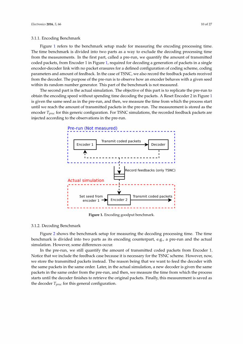
Figure 1 refers to the benchmark setup made for measuring the encoding processing time.The time benchmark is divided into two parts as a way to exclude the decoding processing timefrom the measurements. In the first part, called a pre-run, we quantify the amount of transmittedcoded packets, from Encoder 1 in Figure 1, required for decoding a generation of packets in a singleencoder-decoder link with no packet erasures for a defined configuration of coding scheme, codingparameters and amount of feedback. In the case of TSNC, we also record the feedback packets receivedfrom the decoder. The purpose of the pre-run is to observe how an encoder behaves with a given seedwithin its random number generator. This part of the benchmark is not measured.

The second part is the actual simulation. The objective of this part is to replicate the pre-run toobtain the encoding speed without spending time decoding the packets. A Reset Encoder 2 in Figure 1is given the same seed as in the pre-run, and then, we measure the time from which the process startuntil we reach the amount of transmitted packets in the pre-run. The measurement is stored as theencoder Tproc for this generic configuration. For TSNC simulations, the recorded feedback packets areinjected according to the observations in the pre-run.

Figure 1. Encoding goodput benchmark.

3.1.2. Decoding Benchmark

Figure 2 shows the benchmark setup for measuring the decoding processing time. The timebenchmark is divided into two parts as its encoding counterpart, e.g., a pre-run and the actualsimulation. However, some differences occur.

In the pre-run, we still quantify the amount of transmitted coded packets from Encoder 1.Notice that we include the feedback case because it is necessary for the TSNC scheme. However, now,we store the transmitted packets instead. The reason being that we want to feed the decoder withthe same packets in the same order. Later, in the actual simulation, a new decoder is given the samepackets in the same order from the pre-run, and then, we measure the time from which the processstarts until the decoder finishes to retrieve the original packets. Finally, this measurement is saved asthe decoder Tproc for this general configuration.


Figure 2. Decoding goodput benchmark.

3.2. Energetic Expenditure

In large-scale networks where several Raspis might be deployed, both average power and energyper bit consumption of the devices are relevant parameters that impact the network performance fora given coding scheme. Hence, we consider a study of these energy expenditure parameters for theencoding and decoding. We define these metrics and propose a setup to measure them.

The average power specifies the rate at which energy is consumed in the Raspi. Thus, for a givenenergy value in the device battery without any external supplies, this metric permits one to inferthe amount of time for which the Raspi can operate autonomously before draining out its battery.For the energy per bit consumption, it indicates how much energy is expended to effectively transmitor receive one bit of information taking into account the encoding or decoding operations, respectively.

For our energy measurement campaign, we automate the setup presented in Figure 3 tosequentially run a series of simulations for a given configuration of a coding scheme and its parameters,to estimate the energetic expenditure in both of our Raspi models. The energy measurement setupgoal is to quantify the energy consumption of the Raspi over long periods of processing time to obtainaccurate results. A representative sketch of the setup is shown on the computer monitor in Figure 3.

The energy measurement setup presents a Raspi device whose power supply is an Agilent 66319DDirect Current (DC) source, instead of a conventional power chord supply. To compute the power, wejust need to measure the current, since the Raspi feeds from a fixed input voltage of 5 V set by theAgilent device, but its electric current demand is variable. Hence, the measured variable is the currentconsumed by the device for this fixed input voltage. The output of the measurements are later sent toa workstation where the raw measurement data are processed.

Figure 3. Energy measurement setup.

To identify each experiment, we classified the electrical current samples into two groups basedon the magnitude. In our measurements, the groups to be reported are the idle current Iidle and theprocessing current Iproc. The former is the current the Raspi requires while in idle state, meaning thatno processing is being carried out. The latter stands for the current needed during the encoding or


decoding processing of the packets. Measurements are taken either when Iidle or Iproc are observed.For the processing currents, its current measurements are made while the goodput benchmarks arerunning for a given configuration of a coding scheme with its parameters. For each configuration,103 simulations from the goodput benchmarks are carried out during the period of time where Iproc

occurs. We remark that a simulation is the conveying of g linearly-independent coded packets. Finally,for each configuration, each set of current measurements is enumerated to map it with its averagepower value and the corresponding goodput measurements. At post-processing, from the averagepower expenditure and the results from the goodput measurements, it is possible to extract the energyper bit consumption. We elaborate further on this post-processing in the next subsections.

3.2.1. Average Power Expenditure

To extract the average power for a given configuration in our setup, we first calculate the averagecurrent in the idle state Iidle,avg and the processing state Iproc,avg for all of the available sample for thegiven configuration. Regardless of the current type, the average value of the sample set of a givennumber of samples Ns is:

Iavg =1

Ns

Ns

∑k = 1

Ik [Ampere] (15)

With the average current from (15), we compute the average current used for processing withrespect to the idle state, by subtracting Iidle,avg from Iproc,avg. Then, the result is multiplied by thesupply voltage to obtain the average power during the considered configuration, given as:

Pavg = Vsupply(Iproc,avg − Iidle,avg) [Watt] (16)

3.2.2. Energy per Bit Consumption

To get this metric for a given configuration, we express the energy as the product of theaverage power by the processing time Tproc (s/byte) obtained from the goodput measurement for thesame configuration. In this way, we can relate the processing time with the goodput, the packet andthe generation size as shown:

Eb = PavgTproc,bit = Pavg ×Tproc

8gB=

Pavg

8Rproc[Joule] (17)

4. Measurements and Discussion

With the methodology and setups from the previous sections, we proceed to obtain themeasurements for the Raspi 1 and 2 devices. We consider the following set of parameters forour study: For all of the codes, we use g = [16, 32, 64, 128, 256, 512] and q = [2, 28].For the single-core implementations and cases when the generation size is varied,B = 1600 bytes. We consider another setup where only the packet size varies, B = [64, 128,256, 512, 1024, 2048, 4096, 8192, 16, 384, 32, 768, 65, 536, 131, 072] bytes with a generation size fixed ong = [16, 128] to see the performance of the Raspis in low and high packet size regimes. The thirdsetup we considered used B = 1536 bytes for the optimized multicore implementation. SRLNC wasmeasured with the densities d = [0.02, 0.1]. For TSNC, we considered excess packets, e = [8, 16],so that the budget is b = g + e. In all our measurement reports, to simplify their review, we firstpresent the results for the Raspi 1 and later continue with the Raspi 2.

4.1. Goodput

For the goodput, we separate the results according to their time benchmarks as we did in Section 3.We proceed first with the measurements related to the encoder and later review the case of the decoder.


4.1.1. Encoding

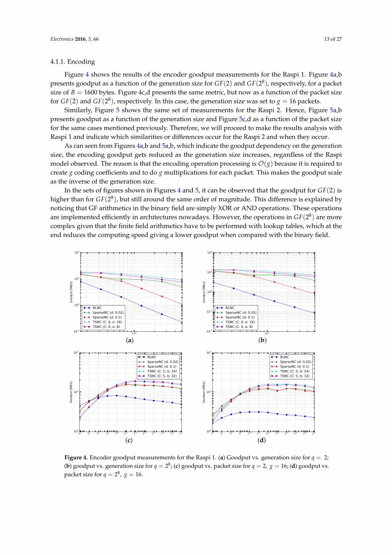
Figure 4 shows the results of the encoder goodput measurements for the Raspi 1. Figure 4a,bpresents goodput as a function of the generation size for GF(2) and GF(28), respectively, for a packetsize of B = 1600 bytes. Figure 4c,d presents the same metric, but now as a function of the packet sizefor GF(2) and GF(28), respectively. In this case, the generation size was set to g = 16 packets.

Similarly, Figure 5 shows the same set of measurements for the Raspi 2. Hence, Figure 5a,bpresents goodput as a function of the generation size and Figure 5c,d as a function of the packet sizefor the same cases mentioned previously. Therefore, we will proceed to make the results analysis withRaspi 1 and indicate which similarities or differences occur for the Raspi 2 and when they occur.

As can seen from Figures 4a,b and 5a,b, which indicate the goodput dependency on the generationsize, the encoding goodput gets reduced as the generation size increases, regardless of the Raspimodel observed. The reason is that the encoding operation processing is O(g) because it is required tocreate g coding coefficients and to do g multiplications for each packet. This makes the goodput scaleas the inverse of the generation size.

In the sets of figures shown in Figures 4 and 5, it can be observed that the goodput for GF(2) ishigher than for GF(28), but still around the same order of magnitude. This difference is explained bynoticing that GF arithmetics in the binary field are simply XOR or AND operations. These operationsare implemented efficiently in architectures nowadays. However, the operations in GF(28) are morecomplex given that the finite field arithmetics have to be performed with lookup tables, which at theend reduces the computing speed giving a lower goodput when compared with the binary field.

102

Generation size

10-1

100

101

102

Goodput [M

B/s]

RLNCSparseNC (d: 0.02)SparseNC (d: 0.1)TSNC (C: 0, e: 16)TSNC (C: 0, e: 8)

(a)102

Generation size

10-2

10-1

100

101

102

Goodput [M

B/s]


(b)

26 27 28 29 210 211 212 213 214 215 216 217

Packet size [B]

100

101

102

Goodput [M

B/s]

RLNCSparseNC (d: 0.02)SparseNC (d: 0.1)TSNC (C: 5, b: 24)TSNC (C: 5, b: 32)

(c)26 27 28 29 210 211 212 213 214 215 216 217

Packet size [B]

100

101

102

Goodput [M

B/s]


(d)

Figure 4. Encoder goodput measurements for the Raspi 1. (a) Goodput vs. generation size for q = 2;(b) goodput vs. generation size for q = 28; (c) goodput vs. packet size for q = 2, g = 16; (d) goodput vs.packet size for q = 28, g = 16.


102

Generation size

100

101

102

Goodput [M

B/s

]


(a)102

Generation size

10-1

100

101

102

Goodput [M

B/s]


(b)

26 27 28 29 210 211 212 213 214 215 216 217

Packet size [B]

100

101

102

103

Goodput [M

B/s]


(c)26 27 28 29 210 211 212 213 214 215 216 217

Packet size [B]

100

101

102

Goodput [M

B/s]


(d)

Figure 5. Encoder goodput measurements for the Raspi 2. (a) Goodput vs. generation size for q = 2;(b) goodput vs. generation size for q = 28; (c) goodput vs. packet size for q = 2, g = 16;(d) goodput vs. packet size for q = 28, g = 16.

In Figures 4a,b and 5a,b, it can be seen that the goodput trends of five codes are a function ofthe generation size: RLNC, SRLNC with d = [0.02, 0.1] and TSNC, with an extra parameter thatwe mention. We define C as the number of density regions in the TSNC transmission process.The maximum number of possible regions depends on the generation size (12). The larger thegeneration, the more density regions may be formed and the more density changes are possible.Throughout this paper, TSNC is configured to use the maximum number of density regions possible.As there can be at least C = 1 density region in a transmission, we use C = 0 to indicate the maximumpossible density regions. This is used for TSNC in plots where the generation size is not fixed. For theplots in the mentioned figures from the encoder goodput measurements, RLNC presents the lowestperformance in terms of goodput and TSNC with e = 16, the highest regardless of the Raspi model.Given that the processing time depends on the amount of coded packets required to be created, RLNCis the slowest to process since it must use all of the g original packets. Later, sparse codes process thedata at a larger rate since less packets are being mixed when creating a coded packet. The caveat ofthese schemes is that the sparser the code, the more probable the occurrences of linearly-dependentpackets are. Therefore, basically, the sparser the codes, the more overhead due to the transmissionsof linearly-dependent packets. Excluding the coding coefficients overhead, the overhead due totransmissions of linearly-dependent packets might be high for the sparse schemes. For example, if weconsider TSNC with e = 16 and g = 16 in Figure 4a, the budget in this case permits one to send upto 32 packets, which is 2× the generation size for an overhead of 100% excluding the overhead fromappending the coding coefficients. This happens because TSNC has been allowed to add too muchredundancy in this case. For RLNC, this is not the case, since the occurrence of linearly-dependentcoded packets is small, because all coding coefficients are used. Even for GF(2), the average amount ofredundant packets for RLNC has been proven to be 1.6 packets after g have been transmitted [41,42],


but less than the cases where sparse codes are utilized. Overall, we observe that there is a trade-offbetween goodput and linearly-dependent coded packets’ transmission overhead.

For Figures 4c,d and 5c,d, we see the packet size effect in the encoding goodput in both Raspimodels and for a fixed generation size. For TSNC in this case, we allow for five density changes duringthe generation transmission and again consider the same budgets as before. In all of the cases, weobserve that there is an optimal packet size with which to operate. When reviewing the specificationsof the Raspi 1, it uses an L1 cache of 16 KiB. Hence, the trends in the packet size can be explained inthe following way: For low packet sizes, the data processing does not overload the Central ProcessingUnit (CPU) of the Raspi, so the goodput progressively increases given that we process more data asthe packet size increases. However, after a certain packet size, the goodput gets affected, since thecache starts to saturate. The packets towards the cache needs to have more processing. Beyond thiscritical packet size, the CPU just queues processing, which incurs larger delay reducing the goodput.

If we consider the previous effect when reviewing the trends in the mentioned figures, in all ofthe models, we observe that the maximum coding performance is not at 16 KiB, but at a smaller valuedepending on the model, field size and coding scheme considered. The reason is that the CPU needsto allocate computational resources to other processes from the different tasks running in the Raspi.Then, given that there are various tasks from other applications for proper functioning running in theRaspi at the same time as coding, the cache space is filled also with the data from these tasks, thusdiminishing the cache space available for coding operations.

For the Raspi 1 model, we observe in Figure 4c that the critical packet size for RLNC using GF(2)occurs at 1 KiB, whereas for the sparse codes, it is close to 8 KiB in most cases for GF(2). This differencetakes place since the sparse codes mix less packets than RLNC, which turns into less data loading inthe cache for doing computations. For a density of d = 0.1, a packet size of B = 8 KiB and g = 16packets, we observe that roughly dgde = 2 packets are inserted in the cache when calculating a codedpacket with this sparse code. Loading this into the cache, this stands for 16 KiB, which is the cache size.A similar effect occurs for the other sparse codes. However, for RLNC given that it is a dense codesince d→ 1, RLNC packets load data from all of the g = 16 coding coefficients, which accounts for the16 KiB of the cache size. In Figure 4d, although the ideal packet size remains the same for RLNC andthe sparse codes, the final goodput is lower due to the field size effect.

The effects mentioned for the Raspi 1 were also observed for the Raspi 2 as mentioned previously.Still, the Raspi 2 achieves roughly 5× to 7× gains in terms of encoding speed when comparing thegoodputs in Figures 4 and 5, given that it has an ARM Cortex A7 (v7) CPU and twice the RandomAccess Memory (RAM) size than the ARM1176JZF-S (v6) core of the Raspi 1 model.

In Figure 5c,d, we observe that the packet size for the maximum RLNC goodput has shiftedtowards 8 KiB, indicating that the Raspi 2 is able to handle 16× 8 KiB = 128 KiB. This is possiblebecause the Raspi 2 has a shared L2 cache of 256 KiB allowing it to still allocate some space for thedata to be processed while achieving a maximum goodput of 105 MB/s.

4.1.2. Decoding

Similar to the encoding goodput, in this section, we review decoder goodput in terms ofperformance and configurations. Figure 6 shows the results of the decoder goodput measurements forthe Raspi 1 and Figure 7 for the Raspi 2.

In Figures 6 and 7, we observe the same generation and packet size effects reported in theencoding case. However, we do observe in Figures 6a,b and 7a,b that doubling the generation sizedoes not reduce the goodput by a factor of four. In principle, given that Gaussian eliminationscales as O(g3) (and thus, the processing time), we would expect the goodput to scale asO(Rproc,dec) = O(g/g3) = O(g−2). This would imply that doubling the generation size shouldreduce the goodput by a factor of four, which is not the case. Instead, the goodput is only reduced bya factor of two. This is only possible if the Gaussian elimination is O(g2). A study in [23] for RLNCspeeds in commercial devices indicated that this is effectively the case. The reason is that the g2 scaling


factor in the scaling law of the Gaussian elimination is much higher than the g3 scaling for g < 512.Particularly, this factor relates to the number of field elements in a packet size as mentioned in [23].

Another difference with the encoding goodput resulting in the same figures is that eventhough TSNC with e = 16 packets provides the fastest encoding, it does not happen to be thesame for the decoding. For this very sparse scheme, the decoding is affected by the amount oflinearly-dependent packets generated, which leads to a higher delay in some cases (particularly ing = [64, 128]). For other generation sizes, the performance of sparse codes is similar.

102

Generation size

10-1

100

101

102

Goodput [M

B/s]


(a)

102

Generation size

10-2

10-1

100

101

Goodput [M

B/s]


(b)

26 27 28 29 210 211 212 213 214 215 216 217

Packet size [B]

100

101

102

Goodput [M

B/s]


(c)

26 27 28 29 210 211 212 213 214 215 216 217

Packet size [B]

100

101

Goodput [M

B/s]


(d)

Figure 6. Decoder goodput measurements for the Raspi 1. (a) Goodput vs. generation size for q = 2;(b) goodput vs. generation size for q = 28; (c) goodput vs. packet size for q = 2, g = 16;(d) goodput vs. packet size for q = 28, g = 16.

102

Generation size

100

101

102

103

Goodput [M

B/s]


(a)

102

Generation size

10-1

100

101

102

Goodput [M

B/s]


(b)

Figure 7. Cont.


26 27 28 29 210 211 212 213 214 215 216 217

Packet size [B]

101

102

103

Goodput [M

B/s]


(c)

26 27 28 29 210 211 212 213 214 215 216 217

Packet size [B]

100

101

102

Goodput [M

B/s]


(d)

Figure 7. Decoder goodput measurements for the Raspi 2. (a) Goodput vs. generation size for q = 2;(b) goodput vs. generation size for q = 28; (c) goodput vs. packet size for q = 2, g = 16; (d) goodput vs.packet size for q = 28, g = 16.

4.2. Average Power

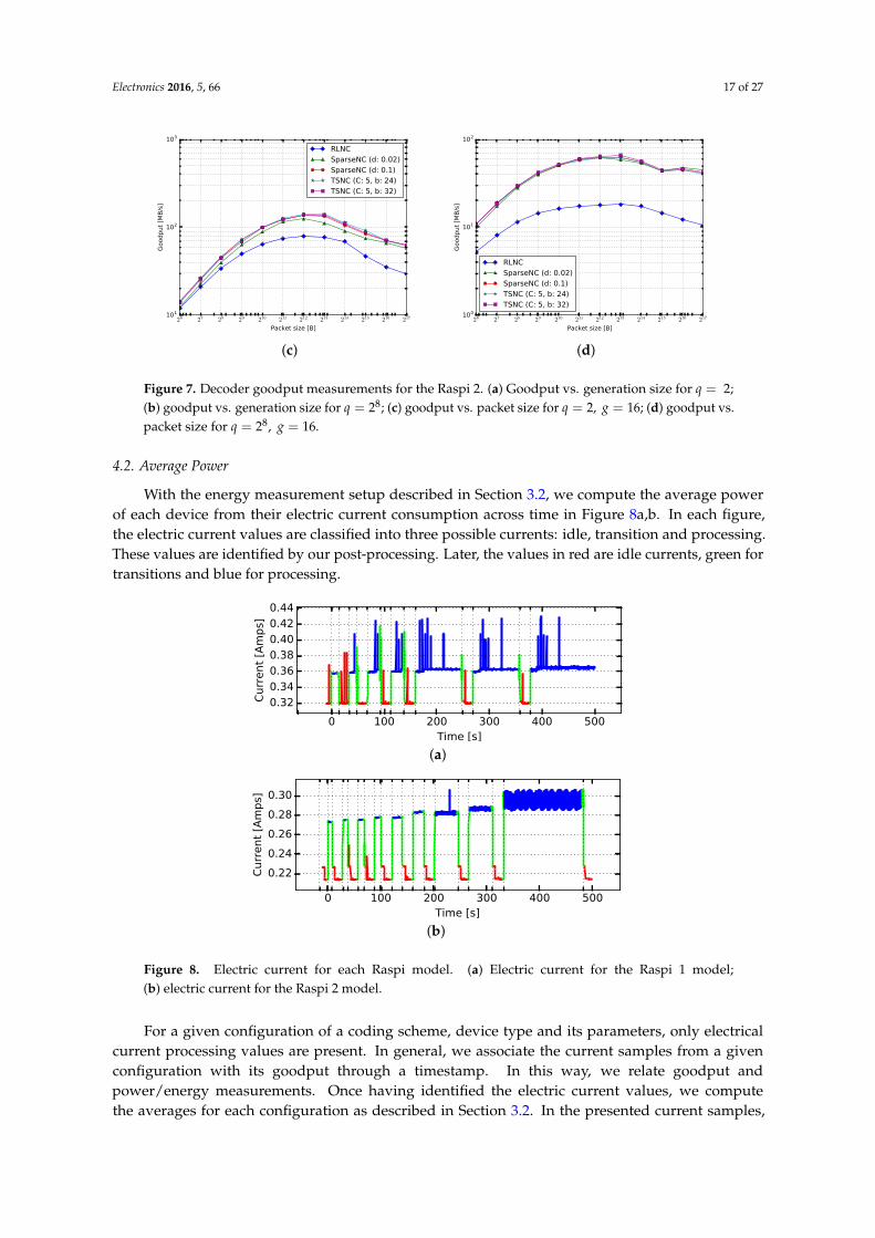
With the energy measurement setup described in Section 3.2, we compute the average powerof each device from their electric current consumption across time in Figure 8a,b. In each figure,the electric current values are classified into three possible currents: idle, transition and processing.These values are identified by our post-processing. Later, the values in red are idle currents, green fortransitions and blue for processing.

0 100 200 300 400 500Time [s]

0.32

0.34

0.36

0.38

0.40

0.42

0.44

Current [Amps]

(a)

0 100 200 300 400 500Time [s]

0.22

0.24

0.26

0.28

0.30

Current [Amps]

(b)

Figure 8. Electric current for each Raspi model. (a) Electric current for the Raspi 1 model;(b) electric current for the Raspi 2 model.

For a given configuration of a coding scheme, device type and its parameters, only electricalcurrent processing values are present. In general, we associate the current samples from a givenconfiguration with its goodput through a timestamp. In this way, we relate goodput andpower/energy measurements. Once having identified the electric current values, we computethe averages for each configuration as described in Section 3.2. In the presented current samples,


we observe the presence of bursty noise. Nevertheless, by taking the average as described in (15),we remove this contribution in the average processing current.

By reviewing the processing current samples in Figure 8a,b, we observe that the averageprocessing current does not change significantly for each Raspi model in all of the shown configurations.Therefore, we approximate the electric current consumption for the devices and compute the averagepower as indicated in (16). The results are shown in Table 1.

Table 1. Average power for the Raspi models.

Raspi Model Iidle,avg (A) Iproc,avg (A) Pavg (W)

Raspi 1 0.320 0.360 0.200Raspi 2 0.216 0.285 0.345

From Table 1, we notice that the power expenditure for both models is almost the same. Thus, theenergy behavior is mostly dependent on the goodput trends, since the power is just a scaling constant.

4.3. Energy per Bit

With power and goodput measurements, we compute the energy per bit of thepreviously-mentioned cases as described in (17). The trends of the energy per bit are the inverse ofthe goodput since both metrics are related by an inverse law. As made with the goodput, we separatethe result descriptions according to the operation carried out by the Raspi: encoding and decoding.Besides this, we differentiate between the models in our study. The energy per bit consumptionremoves the dependency on the amount of packets, helping to normalize the results and indicatingenergy consumption on a fair basis for all of the configurations and coding operations involved inthe study.

4.3.1. Encoding

Figures 9 and 10 show the encoding energy per bit measurements for the Raspi 1 and 2models, respectively. We now proceed to analyze first the Raspi 1 case pointing out proper differenceswith the Raspi 2 when applicable.

In Figure 9a,b, we see the dependency of the energy per bit processed on the generation size forthe Raspi 1 model. In these types of plots, incrementing the generation size incurs more processingtime per byte sent, which leads to more processing time per bit sent. For RLNC, the energy trendsscale as the processing time scales, which is O(g). For sparse codes, this trend is scaled by the density,thus for sparse, we have O(dgde), which can be appreciated in the same figures. We do also noticethat using GF(2) is energy-wise efficient on a per-bit basis since less operations are used to performthe GF arithmetics, which reduces the amount of energy spent.

In Figure 9c,d for the same device, we exhibit the relationship between the energy per bit processedon the packet size, which is the inverse of the goodput vs. the packet size scaling law. We set g = 128 inthis case to observe energy per bit consumption in the regime where the processing time is considerable.As we notice again in this case, GF(2) presents as the field with the smallest energy per bit consumptiongiven that is the one that has the least complex operations. The trends for the energy can be explainedas follows: As the packet size increases, we process more coded bits at the same time, which increasesthe encoding speed, until we hit the critical packet size. After this value, we spend more time queueingdata towards the cache besides the processing, which increases the time spent per processed bit and,thus, the energy.

In Figure 10a–d, we show the encoding energy per bit consumption for the Raspi 2. We clearlysee that the effects discussed for the Raspi 1 also apply as well for the Raspi 2. Moreover, given thatthe average power is in the same order, but the Raspi 2 is a faster device, the energy costs for theRaspi 2 are 2× less than the Raspi 1 when referring to variable generation sizes and a fixed packet size.


Furthermore, these costs are one order of magnitude less for the Raspi 2 with respect to the Raspi 1regarding the case of a fixed generation size and a variable packet size. This makes the Raspi 2achieve a minimum encoding energy consumption per bit processed of 0.2 nJ for the binary field in thementioned regime.

102

Generation size

10-4

10-3

10-2

10-1

Energy per bit [uJ/bit]

RLNCSparseNC (d: 0.02)SparseNC (d: 0.1)TSNC (C: 0, e: 16.0)TSNC (C: 0, e: 8.0)

(a)

102

Generation size

10-4

10-3

10-2

10-1

100



(b)

26 27 28 29 210 211 212 213 214 215 216 217

Packet size [Bytes]

10-4

10-3

10-2

10-1


RLNCSparseNC (d: 0.02)SparseNC (d: 0.1)TSNC (C: 8, b: 136.0)TSNC (C: 8, b: 144.0)

(c)

26 27 28 29 210 211 212 213 214 215 216 217

Packet size [Bytes]

10-3

10-2

10-1



(d)

Figure 9. Encoder energy measurements for the Raspi 1. (a) Energy per bit vs. generation size for q = 2;(b) energy per bit vs. generation size for q = 28; (c) energy per bit vs. packet size for q = 2, g = 128;(d) energy per bit vs. packet size for q = 28, g = 128.

102

Generation size

10-4

10-3

10-2

10-1



(a)

102

Generation size

10-4

10-3

10-2

10-1



(b)

Figure 10. Cont.


26 27 28 29 210 211 212 213 214 215 216 217

Packet size [Bytes]

10-4

10-3

10-2



(c)

26 27 28 29 210 211 212 213 214 215 216 217

Packet size [Bytes]

10-4

10-3

10-2

10-1



(d)

Figure 10. Encoder energy measurements for the Raspi 2. (a) Energy per bit vs. generation sizefor q = 2; (b) energy per bit vs. generation size for q = 28; (c) energy per bit vs. packet size forq = 2, g = 128; (d) energy per bit vs. packet size for q = 28, g = 128.

4.3.2. Decoding

In Figure 11a–d, we show the encoding energy per bit consumption for the Raspi 1. Again, wenotice very similar behavior and trends as previously reviewed for the encoding energy perbit expenditure. In this case, we focus on performance among the coding schemes since the behaviorand trends were previously explained for the encoding case. Later, we introduce the decoding energyresults for the Raspi 2 doing relevant comparisons with the Raspi 1.

Some differences occur due to the nature of decoding. In this situation, the reception oflinearly-dependent coded packets just increases the decoding delay, therefore reducing the performanceof some coding schemes in terms of the energy per bit consumption. For example, we notice thatusing SRLNC with d = 0.02 outperforms TSNC with C = 0 and e = 16, for most of the cases of thevariable generation size curves and in all of the cases of the variable packet size curves of Figure 11.This is a clear scenario, where the decoding delay is energy-wise susceptible to the transmissions oflinearly-dependent coded packets. With the Raspi 1, decoding energies per processed bit of 2 nJ orsimilar are possible.

102

Generation size

10-4

10-3

10-2

10-1



(a)

102

Generation size

10-3

10-2

10-1

100



(b)

Figure 11. Cont.


26 27 28 29 210 211 212 213 214 215 216 217

Packet size [Bytes]

10-3

10-2

10-1



(c)

26 27 28 29 210 211 212 213 214 215 216 217

Packet size [Bytes]

10-3

10-2

10-1



(d)

Figure 11. Encoder energy measurements for the Raspi 1. (a) Energy per bit vs. generation sizefor q = 2; (b) energy per bit vs. generation size for q = 28; (c) energy per bit vs. packet size forq = 2, g = 128; (d) energy per bit vs. packet size for q = 28, g = 128.

Finally, in Figure 12a–d; we introduce the decoding energy per bit consumption for the Raspi 2.Here, we obtain a reduction of an order of magnitude in energy per processed bit due to the speedof the Raspi 2. For example, it can be seen that for the binary field with g = 16 packets, we achievea decoding energy consumption per bit processed close to 0.1 nJ in practical systems.

102

Generation size

10-4

10-3

10-2

10-1



(a)

102

Generation size

10-4

10-3

10-2

10-1



(b)

26 27 28 29 210 211 212 213 214 215 216 217

Packet size [Bytes]

10-4

10-3

10-2



(c)

26 27 28 29 210 211 212 213 214 215 216 217

Packet size [Bytes]

10-4

10-3

10-2

10-1



(d)

Figure 12. Decoder energy measurements for the Raspi 2. (a) Energy per bit vs. generation sizefor q = 2; (b) energy per bit vs. generation size for q = 28; (c) energy per bit vs. packet size forq = 2, g = 128; (d) energy per bit vs. packet size for q = 28, g = 128.


4.4. Multicore Network Coding

To review the performance of NC in a multicore architecture, we implemented the algorithmdescribed in Section 2.4 on the Raspi 2 Model B, which features four ARMv7 cores in a BroadcomBCM2836 System on Chip (SOC) with a 900-MHz clock. Each core has a 32-KiB L1 data cache anda 32-KiB L1 instruction cache. The cores share a 512-KiB L2 cache. All of the measured results,including the baseline results, were obtained with NEON enabled. The Raspi 2 has a NEONextension instruction set, which provides 128-bit SIMD instructions that speed the computations.Figures 13–15 show the encoding and decoding goodput in MB per second for different generation sizes,g = [1024, 128, 16], respectively. For g = [128, 16], the displayed results are the mean valuesover 1000 measurements, while for g = 1024, they are the mean values over 100 measurements.The size of each coded packet was fixed to 1536 bytes, since that is the typical size of an Ethernetframe. The blocked operations were performed dividing the matrices in squared sub-blocks of16, 32 , 64, . . . , 1024 operands (words in the Galois field) in height and width. The figures show onlyblock sizes of 16× 16 and 128× 128 operands, since with bigger block sizes, the operands do not fit inthe cache. Several test cases are considered and detailed.

4.4.1. Baseline Encoding

The baseline results involve no recording of the Direct Acyclic Graph (DAG) and are performedin a by-the-book fashion. The encoder uses only one thread. The difference between the non-blockedand blocked encoding schemes is that in the blocked scheme, the matrix multiplications are performeddividing the matrices into sub-blocks in order to make the algorithm cache efficient, as described inSection 2.4.

4.4.2. Encoding Blocked

The encoding results are obtained using the method described in Section 2.4. The time recordedincludes the dependencies resolving, creation of the DAG and the task scheduling. In practice, it wouldsuffice to calculate and store this information only once per generation size.

4.4.3. Decoding Blocked

The difference between encoding and decoding is that the decoding task also involves the matrixinversion. Similarly, as with the encoding results, the time recorded includes the dependenciesresolving, the creation of the DAG and the task scheduling. However, to decode, these calculations arealso made for inverting the matrix of coding coefficients.

For g = 1024, the blocked baseline measurements outperforms the non-blocked variant.This means that making the matrix multiplication algorithm cache efficient brings an increase ingoodput by a factor of 3.24. When using the algorithm described in Section 2.4, encoding with fourcores is on average 3.9× faster than with one core. Similarly, decoding with four codes is 3.9× faster,on average, than decoding with a single core. Figure 13 shows that the implemented algorithm, byexploiting cache efficiency and only three extra cores provides a 13× gain compared with traditionalnon-blocked algorithms. With g = 1024, the matrix inversion becomes more expensive than at smallergenerations sizes. Therefore, the decoding goodput is 58% of the encoding goodput.

For g = 128, the differences between the baselines operations show that a blocked algorithm is 8%faster than the non-blocked variant. Encoding with four cores is 2.89× faster than with a single core.Due to the smaller matrix sizes, the gain when using blocked operations in the baselines is not thatsignificant when compared with g = 1024. For the same reason, the matrix inversion is less expensive.As a consequence, the decoding goodput is 46% of the encoding goodput.


Base enc. Base blocked enc. Multithread enc. Multithread dec.Strategy

0.0

0.2

0.4

0.6

0.8

1.0

1.2

Goodput

[MB

/s]

Threads

1.02.04.0

Figure 13. Encoding and decoding performance for g = 1024. Block size: 128× 128.


0

2

4

6

8

10

Goodput

[MB

/s]

Threads

1.02.04.0



0

5

10

15

20

25

30

35

Goodput

[MB

/s]

Threads

1.02.04.0



When g = 16, the gains of blocked operations are negligible compared with the non-blocked ones.The reason behind this behavior is that all of the data fits in the L1 cache. For the scheduled version,since the problem to solve is so small, the gain when using four cores is a factor of 2.45 compared witha single core and 1.46 compared with two cores. Therefore, the practical benefits in using four coresinstead of two are reduced.

The differences in goodput, for all generation sizes, between the blocked baseline and thesingle threaded scheduled measurements are due the time spent resolving the dependencies andthe scheduling overhead. These effects are negligible for big generation sizes, while considerable forsmall matrices. For instance, Figure 15 shows that the encoding speed when using one core with thedescribed algorithm is 78% the encoding speed without the recording and calculation of the DAG.

4.4.4. Comparison of the Load of Matrix Multiplications and Inversions

To compare how much slower the matrix multiplication is with respect to the matrix inversionfor different generation sizes, we ran a set of tests. We used a single core to perform the operations.We changed the generation sizes, performed matrices multiplications and matrix inversions andmeasured the time spent doing so, which we name Tmult and Tinv. We calculate the ratio betweenthese two measured times defined as r = Tmult

Tinv. Table 2 summarizes the results. The bigger the matrix

size, the smaller is the calculated ratio. This means that when the problems are bigger, the decodinggoodput decreases compared with the encoding goodput.

Table 2. Multiplication and inversion run-times for different generation sizes with one thread.

g Tmult (ms) Tinv (ms) r

16 1.495 0.169 8.8

32 5.365 0.514 10.4

64 20.573 2.024 10.1

128 81.357 11.755 6.9

256 326.587 75.451 4.3

512 1354.012 540.469 2.5

1024 5965.284 4373.329 1.3

5. Conclusions

Given the usefulness of the Raspi as a low-complex processing node in large-scale networks andnetwork coding techniques against state-of-the-art routing, we provide a performance evaluation ofnetwork coding schemes focusing on processing speed and energy consumption for two Raspi models.The evaluation includes algorithms that exploit both SIMD instructions and multicore capabilities ofthe Raspi 2. Our measurements show that processing speeds of more than 80 Mbps and 800 Mbps areattainable for the Raspi Model 1 and 2, respectively, for a wide range of network coding configurationsand maintaining a processing energy below 1 nJ/bit (or even an order of magnitude lower) in similarconfigurations. For the use of multithreading, we quantify processing gains ranging from 2× forg = 16 to 13× for g = 1024 when employing four threads each in a different core. Future workin the use of Raspi devices will focus on considering: (i) the performance of the Raspi in scenarioswith synthetic packet losses; (ii) wireless networks where real packet losses can occur; and (iii) othertopologies, such as broadcast or the cooperative scenario, to compare with theoretical results in orderto evaluate the performance of different network codes with the Raspi.

Acknowledgments: This research has been partially financed by the Marie Curie Initial Training Network (ITN)CROSSFIRE project (Grant No. EU-FP7-CROSSFIRE-317126) from the European Commission FP7 framework, theGreen Mobile Cloud project (Grant No. DFF-0602-01372B), the TuneSCode project (Grant No. DFF-1335-00125),


both granted by the Danish Council for Independent Research (Det Frie Forskningsråd), and by the GermanResearch Foundation (DFG) within the Collaborative Research Center SFB 912–HAEC.

Author Contributions: All authors contributed equally to the work.

Conflicts of Interest: The authors declare no conflict of interest.

Abbreviations

The following abbreviations are used in this manuscript:

6LoWPAN IPv6 over low power Wireless Personal Area NetworksARM advanced RISC machineBLAS basic linear algebra subprogramsCPU central processing unitD2D device to deviceDAG direct acyclic graphDC direct currentdof degrees of freedomGB GigabyteGF Galois fieldGPU graphic processing unitIoT Internet of ThingsIP Internet ProtocolLAN local area networkLDPC low density parity checkMAC medium access controlNC network codingNFS network file systemOS operating systemPC personal computerQoE quality of experienceRAM random access memoryRaspi Raspberry PiRLNC random linear network codingSCP secure copySIMD single instruction multiple dataSMP symmetric multiprocessorSOC system on chipSRLNC sparse random linear network codingSSH secure shellTelnet TelnetTSNC tunable sparse network codingUSB Universal Serial Bus

References

1. Evans, D. The Internet of Things: How the Next Evolution of the Internet Is Changing Everything;CISCO White Papers; CISCO: San Jose, CA, USA, 2011; Volume 1, pp. 1–11.

2. Al-Fuqaha, A.; Guizani, M.; Mohammadi, M.; Aledhari, M.; Ayyash, M. Internet of things: A survey onenabling technologies, protocols, and applications. IEEE Commun. Surv. Tutor. 2015, 17, 2347–2376.

3. Vujovic, V.; Maksimovic, M. Raspberry Pi as a Wireless Sensor node: Performances and constraints.In Proceedings of the 2014 37th International Convention on Information and Communication Technology,Electronics and Microelectronics (MIPRO), Opatija, Croatia, 26–30 May 2014; pp. 1013–1018.

4. Kruger, C.P.; Abu-Mahfouz, A.M.; Hancke, G.P. Rapid prototyping of a wireless sensor network gatewayfor the internet of things using off-the-shelf components. In Proceedings of the 2015 IEEE InternationalConference on Industrial Technology (ICIT), Seville, Spain, 17–19 March 2015; pp. 1926–1931.

5. Mahmoud, Q.H.; Qendri, D. The Sensorian IoT platform. In Proceedings of the 2016 13th IEEE AnnualConsumer Communications Networking Conference (CCNC), Las Vegas, NV, USA, 9–12 January 2016;pp. 286–287.


6. Wirtz, H.; Rüth, J.; Serror, M.; Zimmermann, T.; Wehrle, K. Enabling ubiquitous interaction withsmart things. In Proceedings of the 2015 12th Annual IEEE International Conference on Sensing,Communication, and Networking (SECON), Seattle, WA, USA, 22–25 June 2015; pp. 256–264.

7. Alletto, S.; Cucchiara, R.; Fiore, G.D.; Mainetti, L.; Mighali, V.; Patrono, L.; Serra, G. An indoorlocation-aware system for an IoT-based smart museum. IEEE Internet Things J. 2016, 3, 244–253.

8. Jalali, F.; Hinton, K.; Ayre, R.; Alpcan, T.; Tucker, R.S. Fog computing may help to save energy incloud computing. IEEE J. Sel. Areas Commun. 2016, 34, 1728–1739.

9. Ueyama, J.; Freitas, H.; Faical, B.S.; Filho, G.P.R.; Fini, P.; Pessin, G.; Gomes, P.H.; Villas, L.A. Exploiting theuse of unmanned aerial vehicles to provide resilience in wireless sensor networks. IEEE Commun. Mag.2014, 52, 81–87.

10. Ahlswede, R.; Cai, N.; Li, S.Y.; Yeung, R.W. Network information flow. IEEE Trans. Inf. Theory 2000,46, 1204–1216.

11. Koetter, R.; Médard, M. An algebraic approach to network coding. IEEE/ACM Trans. Netw. 2003,11, 782–795.

12. Gallager, R.G. Low-density parity-check codes. IRE Trans. Inf. Theory 1962, 8, 21–28.13. Reed, I.S.; Solomon, G. Polynomial codes over certain finite fields. J. Soc. Ind. Appl. Math. 1960, 8, 300–304.14. Ho, T.; Médard, M.; Koetter, R.; Karger, D.R.; Effros, M.; Shi, J.; Leong, B. A random linear network coding

approach to multicast. IEEE Trans. Inf. Theory 2006, 52, 4413–4430.15. Chachulski, S.; Jennings, M.; Katti, S.; Katabi, D. Trading structure for randomness in wireless

opportunistic routing. SIGCOMM Comput. Commun. Rev. 2007, 37, 169–180.16. Katti, S.; Rahul, H.; Hu, W.; Katabi, D.; Médard, M.; Crowcroft, J. XORs in the air: Practical wireless

network coding. IEEE/ACM Trans. Netw. 2008, 16, 497–510.17. Pedersen, M.V.; Fitzek, F.H. Implementation and performance evaluation of network coding for cooperative

mobile devices. In Proceedings of the 2008 IEEE International Conference on Communications Workshops(ICC Workshops’ 08), Beijing, China, 19–23 May 2008; pp. 91–96.

18. Pedersen, M.; Heide, J.; Fitzek, F. Kodo: An open and research oriented network coding library.In Networking 2011 Workshops; Lecture Notes in Computer Science; Springer: Berlin/Heidelberg, Germany,2011; Volume 6827, pp. 145–152.

19. Hundebøll, M.; Ledet-Pedersen, J.; Heide, J.; Pedersen, M.V.; Rein, S.A.; Fitzek, F.H. Catwoman:Implementation and performance evaluation of IEEE 802.11 based multi-hop networks using networkcoding. In Proceedings of the 2012 76th IEEE Vehicular Technology Conference (VTC Fall), Québec City,QC, Canada, 3–6 September 2012; pp. 1–5.

20. Johnson, D.; Ntlatlapa, N.; Aichele, C. Simple pragmatic approach to mesh routing using BATMAN.In Proceedings of the 2nd IFIP International Symposium on Wireless Communications and InformationTechnology in Developing Countries, CSIR, Pretoria, South Africa, 6–7 October 2008.

21. Pahlevani, P.; Lucani, D.E.; Pedersen, M.V.; Fitzek, F.H. Playncool: Opportunistic network coding for localoptimization of routing in wireless mesh networks. In Proceedings of the 2013 IEEE Globecom Workshops(GC Wkshps), Atlanta, GA, USA, 9–13 December 2013; pp. 812–817.

22. Krigslund, J.; Hansen, J.; Hundebøll, M.; Lucani, D.; Fitzek, F. CORE: COPE with MORE in WirelessMeshed Networks. In Proceedings of the 2013 77th IEEE Vehicular Technology Conference (VTC Spring),Dresden, Germany, 2–5 June 2013; pp. 1–6.

23. Paramanathan, A.; Pedersen, M.; Lucani, D.; Fitzek, F.; Katz, M. Lean and mean: Network coding forcommercial devices. IEEE Wirel. Commun. Mag. 2013, 20, 54–61.

24. Seferoglu, H.; Markopoulou, A.; Ramakrishnan, K.K. I2NC: Intra- and inter-session network coding forunicast flows in wireless networks. In Proceedings of the 30th IEEE International Conference on ComputerCommunications ( INFOCOM), Shanghai, China, 10–15 April 2011; pp. 1035–1043.

25. Paramanathan, A.; Pahlevani, P.; Thorsteinsson, S.; Hundebøll, M.; Lucani, D.; Fitzek, F. Sharing the Pi:Testbed Description and Performance Evaluation of Network Coding on the Raspberry Pi. In Proceedingsof the 2014 IEEE 79th Vehicular Technology Conference, Seoul, Korea, 18–21 May 2014.

26. Chou, P.A.; Wu, Y.; Jain, K. Practical network coding. In Proceedings of the 41st Annual AllertonConference on Communication, Control, and Computing, Monticello, IL, USA, 1–3 October 2003.

27. Fragouli, C.; Le Boudec, J.Y.; Widmer, J. Network coding: An instant primer. ACM SIGCOMM Comput.Commun. Rev. 2006, 36, 63–68.


28. Pedersen, M.V.; Lucani, D.E.; Fitzek, F.H.P.; Soerensen, C.W.; Badr, A.S. Network coding designs suited forthe real world: What works, what doesn’t, what’s promising. In Proceedings of the 2013 IEEE InformationTheory Workshop (ITW), Seville, Spain, 9–13 September 2013; pp. 1–5.

29. Sorensen, C.W.; Badr, A.S.; Cabrera, J.A.; Lucani, D.E.; Heide, J.; Fitzek, F.H.P. A Practical View on TunableSparse Network Coding. In Proceedings of the 21th European Wireless Conference European Wireless,Budapest, Hungary, 20–22 May 2015; pp. 1–6.

30. Feizi, S.; Lucani, D.E.; Médard, M. Tunable sparse network coding. In Proceedings of the 2012 InternationalZurich Seminar on Communications (IZS), Zurich, Switzerland, 29 February–2 March 2012; pp. 107–110.

31. Feizi, S.; Lucani, D.E.; Sorensen, C.W.; Makhdoumi, A.; Medard, M. Tunable sparse network coding formulticast networks. In Proceedings of the 2014 International Symposium on Network Coding (NetCod),Aalborg Oest, Denmark, 27–28 June 2014; pp. 1–6.

32. Shojania, H.; Li, B.; Wang, X. Nuclei: GPU-Accelerated Many-Core Network Coding. In Proceedingsof the IEEE 28th Conference on Computer Communications (INFOCOM 2009), Rio de Janeiro, Brazil,20–25 April 2009; pp. 459–467.

33. Shojania, H.; Li, B. Parallelized progressive network coding with hardware acceleration. In Proceedings ofthe 2007 Fifteenth IEEE International Workshop on Quality of Service, Evanston, IL, USA, 21–22 June 2007;pp. 47–55.

34. Wunderlich, S.; Cabrera, J.; Fitzek, F.H.; Pedersen, M.V. Network coding parallelization based on matrixoperations for multicore architectures. In Proceedings of the 2015 IEEE International Conference onUbiquitous Wireless Broadband (ICUWB), Montreal, QC, Canada, 4–7 October 2015; pp. 1–5.

35. Lawson, C.L.; Hanson, R.J.; Kincaid, D.R.; Krogh, F.T. Basic linear algebra subprograms for Fortran usage.ACM Trans. Math. Softw. (TOMS) 1979, 5, 308–323.

36. Dumas, J.G.; Giorgi, P.; Pernet, C. Dense linear algebra over word-size prime fields: The FFLAS andFFPACK packages. ACM Trans. Math. Softw. (TOMS) 2008, 35, 19.

37. Dumas, J.G.; Gautier, T.; Giesbrecht, M.; Giorgi, P.; Hovinen, B.; Kaltofen, E.; Saunders, B.D.; Turner, W.J.;Villard, G. LinBox: A generic library for exact linear algebra. In Proceedings of the 2002 InternationalCongress of Mathematical Software, Beijing, China, 17–19 August 2002; pp. 40–50.

38. Golub, G.H.; Van Loan, C.F. Matrix Computations; JHU Press: Baltimore, MD, USA, 2012; Volume 3.39. Dongarra, J.; Faverge, M.; Ltaief, H.; Luszczek, P. High performance matrix inversion based on LU

factorization for multicore architectures. In Proceedings of the 2011 ACM International Workshop onMany Task Computing on Grids and Supercomputers (MTAGS ’11), Seattle, WA, USA, 14 November 2011;ACM: New York, NY, USA, 2011; pp. 33–42.

40. Sparse Network Codes Implementation Based in the Kodo Library. Available online: https://github.com/chres/kodo/tree/sparse-feedback2 (accessed on 2 September 2016).

41. Trullols-Cruces, O.; Barcelo-Ordinas, J.M.; Fiore, M. Exact decoding probability under random linearnetwork coding. IEEE Commun. Lett. 2011, 15, 67–69.

42. Zhao, X. Notes on “Exact decoding probability under random linear network coding”. IEEE Commun. Lett.2012, 16, 720–721.

Sample Availability: The testbed and measurements in this publication are both available from the authors.

© 2016 by the authors; licensee MDPI, Basel, Switzerland. This article is an open accessarticle distributed under the terms and conditions of the Creative Commons Attribution(CC-BY) license (http://creativecommons.org/licenses/by/4.0/).

https://github.com/chres/kodo/tree/sparse-feedback2

https://github.com/chres/kodo/tree/sparse-feedback2

http://creativecommons.org/

http://creativecommons.org/licenses/by/4.0/.

On Goodput and Energy Measurements of Network Coding ... · electronics Article On Goodput and...

Documents

Transcript of On Goodput and Energy Measurements of Network Coding ... · electronics Article On Goodput and...