ON GIRARD’S “CANDIDATS DE REDUCTIBILITE”´jean/sngirard.pdf · ON GIRARD’S “CANDIDATS DE...
83
ON GIRARD’S “CANDIDATS DE REDUCTIBILIT ´ E” Jean H. Gallier Department of Computer and Information Science University of Pennsylvania Philadelphia, PA 19104 Chapter in Logic and Computer Science, P. Odifreddi, editor, Academic Press, 1989 November 13, 2012 This research was partially supported by ONR under Grant No. N00014-88-K-0593.
Transcript of ON GIRARD’S “CANDIDATS DE REDUCTIBILITE”´jean/sngirard.pdf · ON GIRARD’S “CANDIDATS DE...

ON GIRARD’S “CANDIDATS DE REDUCTIBILITE”
Jean H. Gallier
Department of Computer and Information ScienceUniversity of PennsylvaniaPhiladelphia, PA 19104
Chapter in Logic and Computer Science,P. Odifreddi, editor, Academic Press, 1989
November 13, 2012
This research was partially supported by ONR under Grant No. N00014-88-K-0593.
ON GIRARD’S “CANDIDATS DE REDUCTIBILITE”
Jean H. Gallier
Abstract: We attempt to elucidate the conditions required on Girard’s candi-
dates of reducibility (in French, “candidats de reductibilite”) in order to establish
certain properties of various typed lambda calculi, such as strong normalization
and Church-Rosser property. We present two generalizations of the candidates
of reducibility, an untyped version in the line of Tait and Mitchell, and a typed
version which is an adaptation of Girard’s original method. As an applica-
tion of this general result, we give two proofs of strong normalization for the
second-order polymorphic lambda calculus under �⌘-reduction (and thus under
�-reduction). We present two sets of conditions for the typed version of the
candidates. The first set consists of conditions similar to those used by Stenlund
(basically the typed version of Tait’s conditions), and the second set consists of
Girard’s original conditions. We also compare these conditions, and prove that
Girard’s conditions are stronger than Tait’s conditions. We give a new proof
of the Church-Rosser theorem for both �-reduction and �⌘-reduction, using the
modified version of Girard’s method. We also compare various proofs that have
appeared in the literature (see section 11). We conclude by sketching the exten-
sion of the above results to Girard’s higher-order polymorphic calculus F!
, and
in appendix 1, to F!
with product types.
i

1 Introduction 1
1 Introduction
In this article, we attempt to elucidate the conditions required on Girard’s candidates of
reducibility (in French, “candidats de reductibilite”) in order to establish certain properties
of various typed lambda calculi, such as strong normalization and Church-Rosser property.
We present two generalizations of the candidates of reducibility, an untyped version in the
line of Tait and Mitchell [37, 24], and a typed version which is an adaptation of Girard’s
original method [9, 10]. As an application of this general result, we give two proofs of
strong normalization for the second-order polymorphic lambda calculus under �⌘-reduction
(and thus under �-reduction). We present two sets of conditions for the typed version
of the candidates: a set of conditions similar to those used by Stenlund [35], (basically
the typed version of Tait’s conditions, Tait 1973 [37]), and Girard’s original conditions
(Girard [10], [11]). We also compare these conditions, and prove that Girard’s conditions
are stronger than Tait’s conditions. We give a new proof of the Church-Rosser theorem for
both �-reduction and �⌘-reduction, using the modified version of Girard’s method. We also
compare various proofs that have appeared in the literature (see section 11). We conclude by
sketching the extension of the above results to Girard’s higher-order polymorphic calculus
F!
, and in appendix 1, to F!
with product types.
It is worth noting that the generalized method of candidates plays an important role in
Breazu-Tannen and Gallier [4], where conservation results conjectured in Breazu-Tannen [3]
are proved about the combination of algebraic rewriting with �⌘-reduction in polymorphic
�-calculi.
Familiarity with the polymorphic typed lambda calculus is not assumed for reading
this article. This explains why we have included some rather lengthy introductory sections.
An expert should probably proceed directly to section 6. On the other hand, a certain
familiarity with the simply-typed lambda calculus will help. Good references on the lambda
calculus include Barendregt [1], Hindley and Seldin [15], Stenlund [35], Girard [11], and Huet
[16, 18]. An extensive discussion of the role and importance of type theory and an exposition
of related results are given in Scedrov [32]. Another excellent introduction to type systems
and their relevance to programming language theory appears in Mitchell [25].
2 Syntax of the Second-Order Polymorphic Lambda Calculus
Our presentation of the Girard/Reynolds second-order lambda calculus [9, 30, 11] is heavily
inspired by Breazu-Tannen and Coquand [2]. Let V be a countably infinite set of type
variables, X a countably infinite set of term variables (for short, variables), and B a set of
base types.
2 ON GIRARD’S “CANDIDATS DE REDUCTIBILITE”
Definition 2.1 The set T of second-order polymorphic type expressions (for short, types)
is defined inductively as follows:
t 2 T , whenever t 2 V,� 2 T , whenever � 2 B,(� ! ⌧) 2 T , whenever �, ⌧ 2 T , and
8t. � 2 T , whenever t 2 V and � 2 T .
In omitting parentheses, we follow the usual convention that! associates to the right,
that is, �1 ! �2 ! . . .�n�1 ! �
n
abbreviates (�1 ! (�2 ! . . . (�n�1 ! �
n
) . . .)). The
subset of T consisting of the type expressions built up inductively from B using only the
type constructor! is called the set of simple types. Obviously, simple types cannot contain
type variables or quantifiers.
Next, we define polymorphic raw terms. Let ⌃ be a set of constant symbols and
Type:⌃ ! T a function assigning a closed polymorphic type (i.e., a type expression con-
taining no free type variable) to every symbol in ⌃.
Definition 2.2 The set P⇤ of polymorphic lambda raw ⌃-terms (for short, polymorphic
raw terms) is defined inductively as follows:
c 2 P⇤, whenever c 2 ⌃,
x 2 P⇤, whenever x 2 X ,
(MN) 2 P⇤, whenever M,N 2 P⇤,
(�x:�. M) 2 P⇤, whenever x 2 X , � 2 T , and M 2 P⇤,
(M�) 2 P⇤, whenever � 2 T and M 2 P⇤,
(⇤t. M) 2 P⇤, whenever t 2 V and M 2 P⇤.
The set of free variables in M will be denoted as FV (M), and the set of free type
variables in M as FV(M). The set of bound variables in M will be denoted as BV (M),
and the set of bound type variables in M as BV(M). The same notation is also used to
denote the sets of free and bound variables in a type.
In omitting parentheses, we follow the usual convention that application associates to
the left, that is, M1M2 . . .Mn�1Mn
is an abbreviation for ((. . . (M1M2) . . .Mn�1)Mn
). The
subset of P⇤ consisting of all terms built up using only the first four clauses of definition
2.2 and only simple types is called the set of simply typed raw terms.
Every polymorphic raw term corresponds to an untyped lambda term obtained by
erasing the types. This technique will be useful in proving strong normalization for the
second-order polymorphic lambda calculus. Thus, we define untyped lambda terms and the
Erase function as follows.
Let ⌃ be a set of constant symbols.

3 Substitution and ↵-equivalence 3
Definition 2.3 The set ⇤ of untyped lambda ⌃-terms (for short, lambda terms) is defined
inductively as follows:
c 2 ⇤, whenever c 2 ⌃,
x 2 ⇤, whenever x 2 X ,
(MN) 2 ⇤, whenever M,N 2 ⇤,
(�x. M) 2 ⇤, whenever x 2 X and M 2 ⇤.
The function Erase:P⇤! ⇤ is defined recursively as follows:
Erase(c) = c, whenever c 2 ⌃,
Erase(x) = x, whenever x 2 X ,
Erase(MN) = Erase(M)Erase(N),
Erase(�x:�. M) = �x. Erase(M),
Erase(M�) = Erase(M),
Erase(⇤t. M) = Erase(M).
Not all polymorphic raw terms are acceptable, only those that type-check. In order
to type-check a raw term, one needs to make assumptions about the types of the (term)
variables free in M . This can be done by introducing type assignments. Then, type-
checking a raw term is done using a proof system working on certain expressions called type
judgments. However, substitution plays a crucial role in specifying the inference rules of
this proof system, and so, we now focus our attention on substitutions.
3 Substitution and ↵-equivalence
We first define the notion of a substitution on polymorphic raw terms.
Definition 3.1 A substitution is a function ':X [ V ! P⇤ [ T such that, '(x) 6= x for
only finitely many x 2 X [ V, '(x) 2 P⇤ for all x 2 X , and '(t) 2 T for all t 2 V. The
finite set {x 2 X [V | '(x) 6= x} is called the domain of the substitution and is denoted by
dom('). If dom(') = {x1, . . . , xn
} and '(xi
) = ui
for every i, 1 i n, the substitution
' is also denoted by [u1/x1, . . . , un
/xn
].
Given any substitution ', any variable y 2 X [V, and any term u 2 P⇤[T , '[y := u]
denotes the substitution such that, for all z 2 X [ V,
'[y := u](z) =
⇢u, if y = z;
'(z), if z 6= y.
We also denote '[x := x] as '�x
. The result of applying a substitution to a raw term or a
type is defined recursively as follows.
4 ON GIRARD’S “CANDIDATS DE REDUCTIBILITE”
Definition 3.2 Given any substitution ':X [ V ! P⇤ [ T , the function b':P⇤ [ T !P⇤ [ T extending ' is defined recursively as follows:
b'(x) = '(x), x 2 X ,
b'(t) = '(t), t 2 V,b'(f) = f, f 2 ⌃,
b'(�) = �, � 2 B,b'(� ! ⌧) = b'(�)! b'(⌧), �, ⌧ 2 T ,
b'(8t. �) = 8t. d'�t
(�), � 2 T , t 2 V,b'(PQ) = b'(P )b'(Q), P,Q 2 P⇤,
b'(M�) = b'(M)b'(�), M 2 P⇤,� 2 T ,
b'(�x:�. M) = �x: b'(�). d'�x
(M), M 2 P⇤,� 2 T , x 2 X ,
b'(⇤t. M) = ⇤t. d'�t
(M), M 2 P⇤, t 2 V.
Given a polymorphic raw term M or a type �, we also denote b'(M) as '(M)
and b'(�) as '(�). Also, if dom(') = {x1, . . . , xn
} ✓ X and ' = [M1/x1, . . . ,Mn
/xn
],
then b'(M) is denoted as M [M1/x1, . . . ,Mn
/xn
]. If dom(') = {t1, . . . , tn} ✓ V and
' = [�1/t1, . . . ,�n
/tn
], then b'(M) is denoted as M [�1/t1, . . . ,�n
/tn
] (If � is a type, then
b'(�) is denoted as �[�1/t1, . . . ,�n
/tn
]).
A substitution of untyped lambda terms is defined as a function ':X ! ⇤ with finite
domain.
Definition 3.3 The extension b':⇤! ⇤ of a substitution ':X ! ⇤ is defined recursively
as follows:
b'(x) = '(x), x 2 X ,
b'(f) = f, f 2 ⌃,
b'(PQ) = b'(P )b'(Q), P,Q 2 ⇤,
b'(�x. M) = �x. d'�x
(M), M 2 ⇤, x 2 X .
The notational conventions used for substitutions on polymorphic raw terms are also
used for substitutions on untyped terms. In particular, if M is any untyped lambda term,
we also denote b'(M) as '(M).
We now have to face the painful task of dealing with ↵-conversion and variable capture
in substitutions. The motivation for ↵-conversion is that we want terms that only di↵er by
the names of their bound variables to have the same behavior (and meaning).

3 Substitution and ↵-equivalence 5
Example 3.4 For example, we would like to consider the terms M1 = ⇤t1. �x1: t1. x1
and M2 = ⇤t2. �x2: t2. x2 to be equivalent. They both represent the “polymorphic identity
function”. This can be handled by defining an equivalence relation ⌘↵
which relates terms
that di↵er only by renaming of their bound variables.
Definition 3.5 The relation �!↵
of immediate ↵-reduction is defined by the following
proof system:
Axioms:
8t. � �!↵
8v. �[v/t] for all v 2 V s.t. v /2 FV(�) [ BV(�)�x:�. M �!
↵
�y:�. M [y/x] for all y 2 X s.t. y /2 FV (M) [BV (M)
⇤t. M �!↵
⇤v. M [v/t] for all v 2 V s.t. v /2 FV(M) [ BV(M)
Inference Rules:
� �!↵
⌧
(� ! �) �!↵
(⌧ ! �)
� �!↵
⌧
(� ! �) �!↵
(� ! ⌧)
� �!↵
⌧
8t. � �!↵
8t. ⌧
M �!↵
N
MQ �!↵
NQ
M �!↵
N
PM �!↵
PN
M �!↵
N
M� �!↵
N�
� �!↵
⌧
M� �!↵
M⌧
M �!↵
N
�x:�. M �!↵
�x:�. N
� �!↵
⌧
�x:�. M �!↵
�x: ⌧. M
M �!↵
N
⇤t. M �!↵
⇤t. N
We define ↵-reduction as the reflexive and transitive closure⇤�!
↵
of �!↵
. Finally, we de-
fine ↵-conversion, also called ↵-equivalence, as the least equivalence relation ⌘↵
containing
�!↵
(⌘↵
= (�!↵
[ �!�1↵
)⇤).1
We have the following lemma showing that ↵-equivalence is “congruential” with re-
spect to the term (and type) constructor operations.
1 Warning: �!↵ is not symmetric!
6 ON GIRARD’S “CANDIDATS DE REDUCTIBILITE”
Lemma 3.6 The following properties hold:
If M1 ⌘↵
M2 and N1 ⌘↵
N2, then M1N1 ⌘↵
M2N2.
If M1 ⌘↵
M2 and �1 ⌘↵
�2, then M1�1 ⌘↵
M2�2.
If M1 ⌘↵
M2 and �1 ⌘↵
�2, then �x:�1. M1 ⌘↵
�x:�2. M2.
If M1 ⌘↵
M2, then ⇤t. M1 ⌘↵
⇤t. M2.
Proof . Straightforward by induction.
Lemma 3.6 allows us to consider the term (and type) constructors as operating on
⌘↵
-equivalence classes. Let us denote the equivalence class of a term M modulo ⌘↵
as
[M ], and the equivalence class of a type � modulo ⌘↵
as [�]. We extend application, type
application, abstraction, and type abstraction, to equivalence classes as follows:
[M1][M2] = [M1M2],
[M ][�] = [M�],
[�x: [�]. [M ]] = [�x:�. M ],
[⇤t. [M ]] = [⇤t. M ].
From now on, we will usually identify a term or a type with its ↵-equivalence class
and simply write M for [M ] and � for [�].
In view of the above, ↵-equivalence should also be extended to substitutions as well. By
this, we mean that we should expect that if M1 ⌘↵
M2 and N1 ⌘↵
N2, then M1[N1/x] ⌘↵
M2[N2/x]. However, this may not be true due to the problem of variable capture. As an
illustration, let M1 = �y:�. x, M2 = �w:�. x, and N1 = N2 = w. We have M1 ⌘↵
M2
and of course N1 ⌘↵
N2, but M1[N1/x] = (�y:�. x)[w/x] = �y:�. w and M2[N2/x] =
(�w:�. x)[w/x] = �w:�. w. However, �y:�. w and �w:�. w are not ↵-equivalent. What
went wrong is that when w was substituted for x in M2 = �w:�. x, it became bound in
the result �w:�. w. We say that w was captured . In order to fix this problem, we need
to only allow substitutions that do not cause variable capture. This can be achieved in
several ways. One solution is to redefine substitution so that bound variables involved in
variable capture are renamed. Essentially, ↵-conversion is incorporated into substitution.
We find this solution rather unclean, and instead, we will define when a term is safe for a
substitution, and use ↵-conversion to get around variable capture.
Given a substitution ':X [ V ! P⇤ [ T , we let FV (') =S
x2dom(') FV ('(x)), and
FV(') =S
x2dom(') FV('(x)).

3 Substitution and ↵-equivalence 7
Definition 3.7 Given a substitution ':X [ V ! P⇤ [ T , given any term M or type �,
safe(',M) and safe(',�) are defined recursively as follows:
safe(', x) = true, x 2 X ,
safe(', t) = true, t 2 V,safe(', f) = true, f 2 ⌃,
safe(',�) = true, � 2 B,safe(',� ! ⌧) = safe(',�) and safe(', ⌧), �, ⌧ 2 T ,
safe(', 8t. �) = safe('�t
,�) and t /2 FV('), � 2 T , t 2 V,safe(', PQ) = safe(', P ) and safe(', Q), P,Q 2 P⇤,
safe(',M�) = safe(',M) and safe(',�), M 2 P⇤,� 2 T ,
safe(',�x:�. M) = safe('�x
,�) and safe('�x
,M) and x /2 FV ('),
M 2 P⇤,� 2 T , x 2 X ,
safe(',⇤t. M) = safe('�t
,M) and t /2 FV('), M 2 P⇤, t 2 V.
When safe(',M) holds we say that M is safe for ', and when safe(',�) holds we
say that � is safe for '.
Given any substitution ' and any term M (or type �), it is immediately seen that
there is some term M 0 (or type �0) such that M ⌘↵
M 0 (� ⌘↵
�0) and M 0 is safe for ' (�0
is safe for '). From now on, it is assumed that terms and types are ↵-renamed before a
substitution is applied, so that the substitution is safe. It is natural to extend ↵-equivalence
to substitutions as follows.
Definition 3.8 Given any two substitutions ' and '0 such dom(') = dom('0), we write
' ⌘↵
' i↵ '(x) ⌘↵
'0(x) for every x 2 dom(').
We have the following lemma.
Lemma 3.9 For any two substitutions ' and '0, terms M , M 0, and types � and �0, if M ,
M 0, �, �0 are safe for ' and '0, ' ⌘↵
'0, M ⌘↵
M 0, and � ⌘↵
�0, then '(M) ⌘↵
'0(M 0),
and '(�) ⌘↵
'0(�0).
Proof . A very tedious induction on terms with many cases corresponding to the definition
of ↵-equivalence.
Corollary 3.10 (i) If (�x:�1. M1)N1 ⌘↵
(�y:�2. M2)N2, M1 is safe for [N1/x], and M2
is safe for [N2/y], then M1[N1/x] ⌘↵
M2[N2/y]. (ii) If (⇤t. M1)⌧1 ⌘↵
(⇤v. M2)⌧2, M1 is
safe for [⌧1/t], and M2 is safe for [⌧2/v], then M1[⌧1/t] ⌘↵
M2[⌧2/v].

8 ON GIRARD’S “CANDIDATS DE REDUCTIBILITE”
We are now ready to present the proof system for type-checking raw terms.
4 Type Assignments and Type-Checking
First, we need the notion of a type assignment.
Definition 4.1 A type assignment is a partial function �:X ! T with a finite domain
denoted as dom(�). Thus, a type assignment � is a finite set of pairs {x1:�1, . . . , xn
:�n
}where the variables are pairwise distinct. Given a type assignment � and a pair hx,�iwhere x 2 X and � 2 T , provided that x /2 dom(�), we write �, x:� for � [ {hx,�i}.
In order to determine whether a raw term type-checks, we attempt to construct a
proof of a typing judgment using the proof system described below.
Definition 4.2 A typing judgment of type � is an expression of the form � .M :�, where
� is a type assignment, M is a polymorphic raw term, and � is a type.
The proof system for deriving typing judgments is the following:
Axioms:
� . c:Type(c), c 2 ⌃ (constants)
� . x:�(x), x 2 dom(�) (variables)
Inference Rules:� .M :� ! ⌧ � .N :�
� .MN : ⌧(application)
�, x:� .M : ⌧
� . (�x:�. M):� ! ⌧(abstraction)
� .M : 8t. �� .M⌧ :�[⌧/t]
(type application)
where � is safe for the substitution [⌧/t]
� .M :�
� . (⇤t. M): 8t. �(type abstraction)
where in this last rule, t /2 FV(�(x)) for every x 2 dom(�) \ FV (M).
If � .M :� is provable using the above proof system, we say that M type-checks with
type � under � and we write ` � .M :�. We say that the raw term M type-checks under
4 Type Assignments and Type-Checking 9
� i↵ there exists some type � such that � .M :� is derivable. Finally, we say that the raw
term M type-checks (or is typable) i↵ there is some � and some � such that � . M :� is
derivable.
Note that the terms M1 and M2 of example 3.4 both type-check, since it is easily
shown that ` . ⇤t1. �x1: t1. x1: 8t1. (t1 ! t1) and ` . ⇤t2. �x2: t2. x2: 8t2. (t2 ! t2).
This example suggests that ↵-equivalence should be extended to typing judgments as
well. Indeed, . ⇤t1. �x1: t1. x1: 8t1. (t1 ! t1) and . ⇤t2. �x2: t2. x2: 8t3. (t3 ! t3) should be
considered equivalent. We extend ⌘↵
to typing judgments as follows.
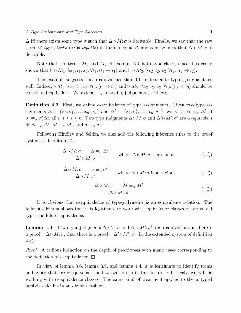
Definition 4.3 First, we define ↵-equivalence of type assignments. Given two type as-
signments � = {x1:�1, . . . , xn
:�n
} and �0 = {x1:�01, . . . , xn
:�0n
}, we write � ⌘↵
�0 i↵
�i
⌘↵
�0i
for all i, 1 i n. Two type judgments �.M :� and �0 .M 0:�0 are ↵-equivalent
i↵ � ⌘↵
�0, M ⌘↵
M 0, and � ⌘↵
�0.
Following Hindley and Seldin, we also add the following inference rules to the proof
system of definition 4.2.
� .M :� � ⌘↵
�0
�0 .M :�where � .M :� is an axiom (⌘0
↵
)
� .M :� � ⌘↵
�0
� .M :�0 where � .M :� is an axiom (⌘00↵
)
� .M :� M ⌘↵
M 0
� .M 0:�(⌘000
↵
)
It is obvious that ↵-equivalence of type-judgments is an equivalence relation. The
following lemma shows that it is legitimate to work with equivalence classes of terms and
types modulo ↵-equivalence.
Lemma 4.4 If two type judgments � .M :� and �0 .M 0:�0 are ↵-equivalent and there is
a proof ` � .M :�, then there is a proof ` �0 .M 0:�0 (in the extended system of definition
4.3).
Proof . A tedious induction on the depth of proof trees with many cases corresponding to
the definition of ↵-equivalence.
In view of lemma 3.6, lemma 3.9, and lemma 4.4, it is legitimate to identify terms
and types that are ↵-equivalent, and we will do so in the future. E↵ectively, we will be
working with ↵-equivalence classes. The same kind of treatment applies to the untyped
lambda calculus in an obvious fashion.

10 ON GIRARD’S “CANDIDATS DE REDUCTIBILITE”
The following lemma shows that the notion of substitution given by definition 3.2 is
type preserving when applied to terms that type-check.
Given a type assignment � = {x1:�1, . . . , xn
:�n
} and a substitution ✓:V ! T , let
✓(�) = {x1: ✓(�1), . . . , xn
: ✓(�n
)}.
Lemma 4.5 (i) For any term M and any substitution ':X ! P⇤ s.t. FV (M) ✓ dom('),
if M type-checks with proof ` �.M : ⌧ , and there is some � such that for every x 2 FV (M),
'(x) type-checks with some proof ` � . '(x):�(x) and M is safe for ', then '(M) type-
checks with some proof ` � . '(M): ⌧ . (ii) For any term M 2 P⇤ and any substitution
✓:V ! T , if M type-checks with proof ` � .M :� and �, M , and � are safe for ✓, then,
✓(M) type-checks with some proof ` ✓(�) . ✓(M): ✓(�).
Proof . Both proofs are tedious but not di�cult. They are left to the courageous readers.
Definition 4.6 Given any contexts �,�, a type-preserving substitution is a function ' :
dom(�) ! P⇤ such that, for every x 2 dom(�), ` � . '(x) : �(x). Such a substitution is
denoted as ' : �! �.
Another useful and tedious lemma shows that substitution of raw terms is preserved
under erasing.
Lemma 4.7 (i) For all raw M,N 2 P⇤, Erase(M [N/x]) = Erase(M)[Erase(N)/x]. (ii)
For every raw term M 2 P⇤ and type ⌧ 2 T , Erase(M [⌧/t]) = Erase(M).
Proof . The proof proceeds by cases and it is tedious but not di�cult.
We are finally ready to define the notion of reduction.
5 Reduction and Conversion
It is convenient to define reduction on raw terms, and verify that it is type-preserving when
applied to a term that type-checks. Actually, we will define reduction on ↵-equivalence
classes and use lemma 3.6 and corollary 3.10 to ensure that this definition makes sense.
Thus, in what follows, terms and types are identified with their ⌘↵
-equivalence class. In
particular, if we consider an equivalence class of the form [(�x:�. M)N ], we can assume
that M has been ↵-renamed so that M is safe for the substitution [N/x], and similarly for
a class of the form [(⇤t. M)⌧ ].

5 Reduction and Conversion 11
Definition 5.1 The relation �!�
8 of immediate reduction is defined in terms of the four
relations �!�
, �!⌘
, �!⌧�
, and �!⌧⌘
, defined by the following proof system:
Axioms:
(�x:�. M)N �!�
M [N/x], provided that M is safe for [N/x] (�)
�x:�. (Mx) �!⌘
M, provided that x /2 FV (M) (⌘)
(⇤t. M)⌧ �!⌧�
M [⌧/t], provided that M is safe for [⌧/t] (type �)
⇤t. (Mt) �!⌧⌘
M, provided that t /2 FV(M) (type ⌘)
Inference Rules: For each kind of reduction �!r
where r 2 {�, ⌘, ⌧�, ⌧⌘},
M �!r
N
MQ �!r
NQ
M �!r
N
PM �!r
PNfor all P,Q 2 P⇤ (congruence)
M �!r
N
M� �!r
N�for all � 2 T (type congruence)
M �!r
N
�x:�. M �!r
�x:�. Nx 2 X ,� 2 T (⇠)
M �!r
N
⇤t. M �!r
⇤t. Nt 2 V (type ⇠)
We define �!�
8 = �!�
[ �!⌘
[ �!⌧�
[ �!⌧⌘
, and reduction as the reflexive and
transitive closure⇤�!
�
8 of �!�
8 . We also define immediate conversion !�
8 such that
!�
8 = �!�
8 [ �!�1�
8 , and conversion as the reflexive and transitive closure⇤ !
�
8 of
!�
8 .
The following lemma shows that reduction is type-preserving.
Lemma 5.2 Given any two raw terms M,N 2 P⇤, if M type-checks with proof ` �.M :�
and M �!�
8 N , then N also type-checks with some proof ` � .N :�.
Proof . Again, the proof proceeds by cases and it is tedious but not di�cult.
It is evident that lemma 5.2 also holds for⇤�!
�
8 .
Reduction and conversion can also be defined for the untyped lambda calculus. The
reduction relation⇤�!
�
is defined by only retaining the � and ⌘ reduction axioms of
definition 5.1, and the inference rules not involving types. The notion of conversion⇤ !
�
is defined from �!�
in the usual way. It is easy to see that an analog of lemma 3.9 holds
12 ON GIRARD’S “CANDIDATS DE REDUCTIBILITE”
for untyped �-terms. When we need to distinguish between a �-reduction step and a �8-
reduction step, we add the name of the calculus as a subscript. For example, �!�,�
is a
�-conversion step in the untyped lambda calculus �, whereas �!�,�
8 is a �-conversion step
in the polymorphic lambda calculus �8.
We have the following lemma showing how a reduction step �!�
8 is mapped to a
reduction step⇤�!
�
by the Erase function.
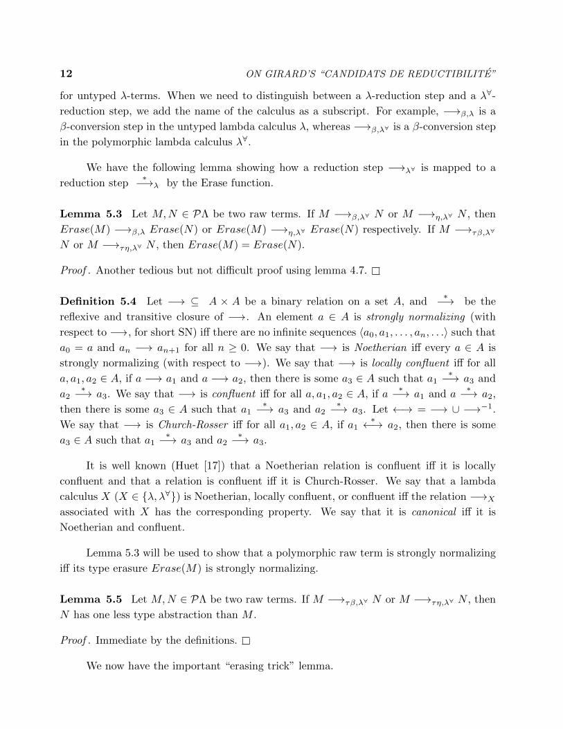
Lemma 5.3 Let M,N 2 P⇤ be two raw terms. If M �!�,�
8 N or M �!⌘,�
8 N , then
Erase(M) �!�,�
Erase(N) or Erase(M) �!⌘,�
8 Erase(N) respectively. If M �!⌧�,�
8
N or M �!⌧⌘,�
8 N , then Erase(M) = Erase(N).
Proof . Another tedious but not di�cult proof using lemma 4.7.
Definition 5.4 Let �! ✓ A ⇥ A be a binary relation on a set A, and⇤�! be the
reflexive and transitive closure of �!. An element a 2 A is strongly normalizing (with
respect to �!, for short SN) i↵ there are no infinite sequences ha0, a1, . . . , an, . . .i such that
a0 = a and an
�! an+1 for all n � 0. We say that �! is Noetherian i↵ every a 2 A is
strongly normalizing (with respect to �!). We say that �! is locally confluent i↵ for all
a, a1, a2 2 A, if a �! a1 and a �! a2, then there is some a3 2 A such that a1⇤�! a3 and
a2⇤�! a3. We say that �! is confluent i↵ for all a, a1, a2 2 A, if a
⇤�! a1 and a⇤�! a2,
then there is some a3 2 A such that a1⇤�! a3 and a2
⇤�! a3. Let ! = �! [ �!�1.
We say that �! is Church-Rosser i↵ for all a1, a2 2 A, if a1⇤ ! a2, then there is some
a3 2 A such that a1⇤�! a3 and a2
⇤�! a3.
It is well known (Huet [17]) that a Noetherian relation is confluent i↵ it is locally
confluent and that a relation is confluent i↵ it is Church-Rosser. We say that a lambda
calculus X (X 2 {�,�8}) is Noetherian, locally confluent, or confluent i↵ the relation �!X
associated with X has the corresponding property. We say that it is canonical i↵ it is
Noetherian and confluent.
Lemma 5.3 will be used to show that a polymorphic raw term is strongly normalizing
i↵ its type erasure Erase(M) is strongly normalizing.
Lemma 5.5 Let M,N 2 P⇤ be two raw terms. If M �!⌧�,�
8 N or M �!⌧⌘,�
8 N , then
N has one less type abstraction than M .
Proof . Immediate by the definitions.
We now have the important “erasing trick” lemma.

6 An Untyped Version of The Candidates of Reducibility 13
Lemma 5.6 Let M 2 P⇤ be any raw term. If there is an infinite sequence of �!�
8
reductions from M , then there is an infinite sequence of �!�
reductions from Erase(M).
Proof . First, observe that any infinite sequence of �!�
8 reductions from M must contain
a subsequence consisting of infinitely many �!�,�
8 or �!⌘,�
8 reductions, since otherwise
some term in this sequence would be the head of an infinite sequence of �!⌧�,�
8 or �!⌧⌘,�
8
reductions, contradicting lemma 5.5. But then, by lemma 5.3, the infinite sequence of
�!�
8 reductions from M maps by Erase to an infinite sequence of �!�
reductions from
Erase(M).
Thus, lemma 5.6 implies that a polymorphic raw term is strongly normalizing i↵ its
type erasure Erase(M) is strongly normalizing. In the next section, it will be shown that
if M is a raw term that type-checks, then Erase(M) is strongly normalizing, thus showing
that M itself is strongly normalizing.2 The following lemma will also be needed.
Lemma 5.7 Let M1,M2, N1, N2 2 ⇤ be untyped lambda terms. If M1⇤�!
�
M2 and
N1⇤�!
�
N2, then M1[N1/x]⇤�!
�
M2[N2/x].
Proof . We use two inductions, one on the structure of M1, and the other on the length of
reduction sequences. The details are quite tedious.
6 An Untyped Version of The Candidates of Reducibility
Originally, the “candidats de reductibilite” were defined by Girard as sets of typed (poly-
morphic) lambda terms with certain closure properties (Girard 1970 [9], Girard 1972 [10]).
Soon after Girard, Tait observed that Girard’s brilliant device could be simplified if the
candidates are defined as certain sets of untyped lambda terms, and if a certain “erasing
trick” is used (Tait 1973 [37]).3 Roughly thirteen years after Tait, Mitchell independently
noticed that an untyped version of the candidates is more flexible to work with, and he gave
his own version generalizing Tait’s version (Mitchell 1986 [24]).
Before we proceed with the technical details, we will attempt to reveal some of the
intuitions underlying the proof. We believe that this is best accomplished by first restricting
our attention to the simply typed lambda calculus. The problem is to show that every simply
typed term that type-checks is strongly normalizing.
2 It is interesting to note that Tait [37] used an erasing trick in his proof, but the definition of hiserasing function is di↵erent from the one given here.
3 Interestingly, the erasing trick was known to Girard himself, since it appears in his thesis, Girard1972 [10]. However, he did not make use of it in his proof of strong normalization.

14 ON GIRARD’S “CANDIDATS DE REDUCTIBILITE”
A natural way of attacking the problem is to attempt a proof by induction on the
size of terms. The base case of a (typed) variable or a (typed) constant works out nicely,
since no reduction applies. The case of a lambda abstraction M = �x:�. N also works fine,
because if any reduction applies to M , then it must in fact apply to N , and N has strictly
smaller size than M , so the induction hypothesis applies. Di�culties arise in case of an
application of the form (�x:�. M)N . The induction hypothesis applies to both �x:�. M
and N , but there is another possibility of reduction, namely (�x:�.M)N �!�
M [N/x], and
unfortunately, M [N/x] is not necessarily strictly smaller than (�x:�. M)N . Tait’s clever
solution for overcoming this problem (Tait [36]) is essentially to strengthen the induction
hypothesis. He does so by defining by induction on types the class of “computable” (or
“reducible”) terms. Let us denote the set of simply typed terms of type � (that type-check)
as ST�
, and the subset of all SN terms in ST�
as SN�
. For every simple type �, the set [[�]]
is a subset of ST�
defined as follows:
(1) [[�]] = SN�
, for every base type �;
(2) [[(� ! ⌧)]] = {M 2 ST(�!⌧) | 8N 2 [[�]], MN 2 [[⌧ ]]}.
One can then prove by induction on types that
[[�]] ✓ SN�
, (a)
that is, all terms in [[�]] are SN. In order to finish the proof, it is su�cient to show that
ST�
✓ [[�]], (b)
since (a) and (b) together prove that ST�
= SN�
.
The way to prove (b) is to proceed by induction on the size of terms. Note that
the problematic case of an application MN (where M 2 ST�!⌧
) is now easy: by the
induction hypothesis, M 2 [[(� ! ⌧)]] and N 2 [[�]], and by the definition of [[(� ! ⌧)]], we
have MN 2 [[⌧ ]]. This time, the di�cult case is to prove that for every term of the form
�x:�. M , where M 2 ST⌧
, �x:�. M 2 [[(� ! ⌧)]]. We need to show that for every N 2 [[�]],
(�x:�. M)N 2 [[⌧ ]]. Since (�x:�. M)N �!�
M [N/x], if we could show that M [N/x] 2 [[⌧ ]]
and that whenever M [N/x] 2 [[⌧ ]], then (�x:�. M)N 2 [[⌧ ]], we would be able to conclude.
This can be done, but it is necessary to strengthen the induction hypothesis. Roughly,
the idea is show that for every term M 2 ST�
, for every substitution ' assigning to each
variable of type ⌧ in M some term in [[⌧ ]], then '(M) 2 [[�]]. Then, we have our result by
choosing ' to be the identity substitution.
Now, it turns out that the sets of the form [[�]] have certain closure properties (proper-
ties (S1), (S2) of definition 6.9) that make the various induction steps go through. Girard’s
6 An Untyped Version of The Candidates of Reducibility 15
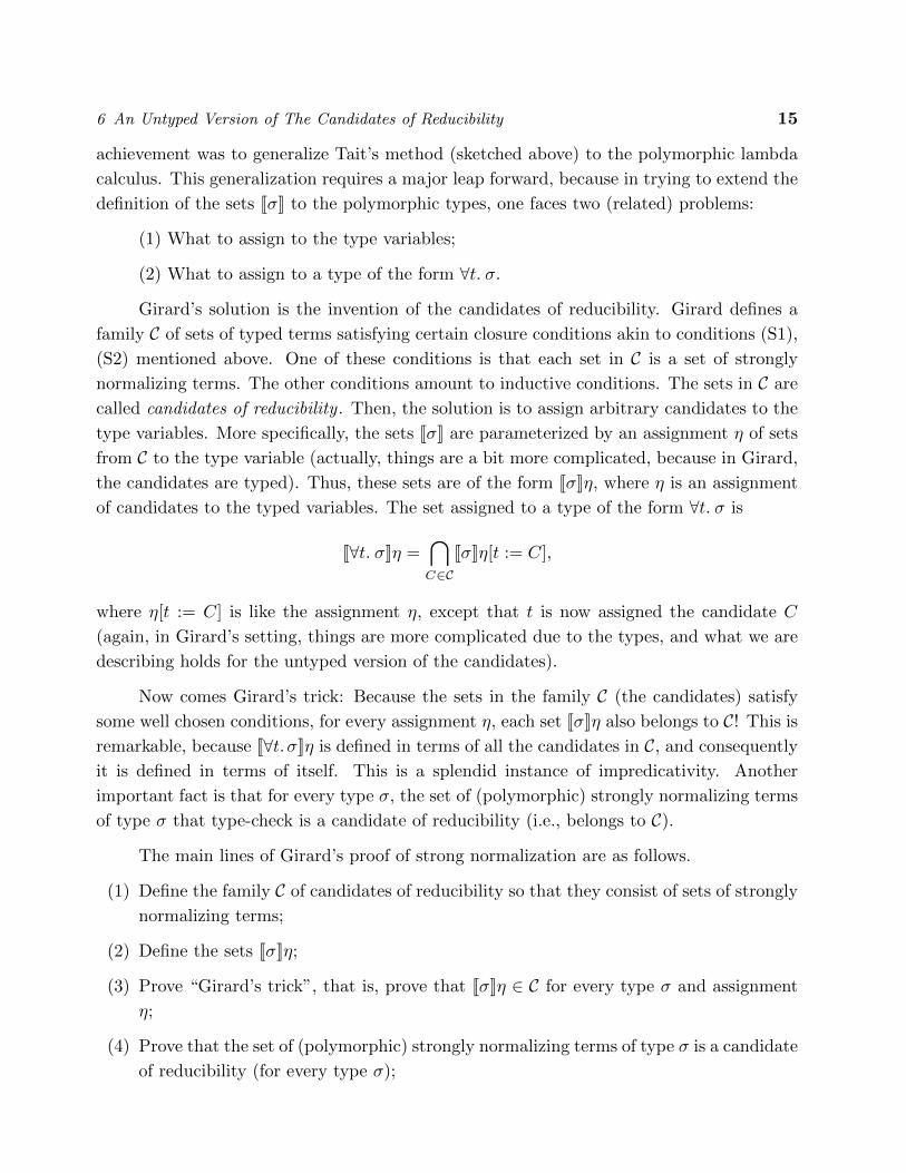
achievement was to generalize Tait’s method (sketched above) to the polymorphic lambda
calculus. This generalization requires a major leap forward, because in trying to extend the
definition of the sets [[�]] to the polymorphic types, one faces two (related) problems:
(1) What to assign to the type variables;
(2) What to assign to a type of the form 8t. �.
Girard’s solution is the invention of the candidates of reducibility. Girard defines a
family C of sets of typed terms satisfying certain closure conditions akin to conditions (S1),
(S2) mentioned above. One of these conditions is that each set in C is a set of strongly
normalizing terms. The other conditions amount to inductive conditions. The sets in C are
called candidates of reducibility . Then, the solution is to assign arbitrary candidates to the
type variables. More specifically, the sets [[�]] are parameterized by an assignment ⌘ of sets
from C to the type variable (actually, things are a bit more complicated, because in Girard,
the candidates are typed). Thus, these sets are of the form [[�]]⌘, where ⌘ is an assignment
of candidates to the typed variables. The set assigned to a type of the form 8t. � is
[[8t. �]]⌘ =\
C2C[[�]]⌘[t := C],
where ⌘[t := C] is like the assignment ⌘, except that t is now assigned the candidate C
(again, in Girard’s setting, things are more complicated due to the types, and what we are
describing holds for the untyped version of the candidates).
Now comes Girard’s trick: Because the sets in the family C (the candidates) satisfy
some well chosen conditions, for every assignment ⌘, each set [[�]]⌘ also belongs to C! This isremarkable, because [[8t.�]]⌘ is defined in terms of all the candidates in C, and consequently
it is defined in terms of itself. This is a splendid instance of impredicativity. Another
important fact is that for every type �, the set of (polymorphic) strongly normalizing terms
of type � that type-check is a candidate of reducibility (i.e., belongs to C).
The main lines of Girard’s proof of strong normalization are as follows.
(1) Define the family C of candidates of reducibility so that they consist of sets of strongly
normalizing terms;
(2) Define the sets [[�]]⌘;
(3) Prove “Girard’s trick”, that is, prove that [[�]]⌘ 2 C for every type � and assignment
⌘;
(4) Prove that the set of (polymorphic) strongly normalizing terms of type � is a candidate
of reducibility (for every type �);

16 ON GIRARD’S “CANDIDATS DE REDUCTIBILITE”
(5) Prove that for every (polymorphic) term M of type � that type-checks, M 2 [[�]]⌘, for
every assignment ⌘.
By choosing the assignment ⌘ so that it assigns to the type variables the sets of terms
that are strongly normalizing, we obtain the desired result: every term that type-checks is
strongly normalizing.
It should be noted that in order to prove (5), one needs a substantially strengthened
induction hypothesis (see lemma 6.8).
We will now prove strong normalization using an untyped version of the candidates
of reducibility, following Mitchell and Tait. We go one step further and define a kind of
abstract version of the candidates of reducibility. This way, it is easier to pinpoint the
ingredients that are crucial to proofs using this concept. We first describe what we referred
to as “Girard’s trick”.
Definition 6.1 Given two sets S and T of (untyped) lambda terms, we let [S ! T ] be
the set of (untyped) lambda terms defined as follows:
[S ! T ] = {M 2 ⇤ | 8N 2 S, MN 2 T}.
We refer to the operation ! on sets of lambda terms defined above as the function space
constructor .
Definition 6.2 Let C be a nonempty family of sets of (untyped) lambda terms having the
following properties:
(1) Every C 2 C is nonempty.
(2) C is closed under the function space constructor.
(3) Given any C-indexed family (AC
)C2C of sets in C, then
TC2C AC
2 C.
A family satisfying the above conditions is called a T -closed family .4
We shall prove shortly that such families exist.
Let C be a T -closed family. Given any assignment ⌘:B[V ! C of sets in C to the type
variables and the base types, we can associate certain sets of lambda terms to the types
inductively as explained below. In the following definition, given any set C 2 C and any
type variable t, ⌘[t := C] denotes the assignment such that, for all v 2 V,
⌘[t := C](v) =
⇢C, if v = t;
⌘(v), if v 6= t.
4 In all rigor, we also have to assume that every C 2 C is closed under ↵-equivalence.

6 An Untyped Version of The Candidates of Reducibility 17
Definition 6.3 Given any assignment ⌘:B [ V ! C, for every type �, the set [[�]]⌘ is
defined as follows:
[[t]]⌘ = ⌘(t), whenever t 2 B [ V,
[[(� ! ⌧)]]⌘ = [[[�]]⌘ ! [[⌧ ]]⌘] (where! is the function space contructor defined earlier);
[[8t. �]]⌘ =T
C2C [[�]]⌘[t := C].
The following technical lemma will be useful later.
Lemma 6.4 Given any two assignments ⌘1:B [ V ! C and ⌘2:B [ V ! C, for every type
�, if ⌘1 and ⌘2 agree on FV(�) and B, then [[�]]⌘1 = [[�]]⌘2.
Proof . Easy induction on the structure of types.
The next result constitutes the essence of “Girard’s trick”.
Lemma 6.5 (Girard) If C is a T -closed family, for every assignment ⌘:B [ V ! C, forevery type �, then [[�]]⌘ 2 C.
Proof . The lemma is proved by induction on the structure of types. The case of a type
variable or a base type t is obvious since by the definition [[t]]⌘ = ⌘(t).
For a type (� ! ⌧), by the induction hypothesis we have [[�]]⌘ 2 C and [[⌧ ]]⌘ 2 C, andby condition (2) of T -closed families, we also have [[[�]]⌘ ! [[⌧ ]]⌘] 2 C.
For a type 8t. �, by the induction hypothesis, for every assignment µ:B [ V ! C,[[�]]µ 2 C. Thus, for every C 2 C we also have [[�]]⌘[t := C] 2 C, since ⌘[t := C] is an
assignment. By condition (3) of T -closed families, we haveT
C2C [[�]]⌘[t := C] 2 C.
The following technical lemma will be needed later.
Lemma 6.6 Given any two types �, ⌧ , for every assignment ⌘:B [ V ! C, if � is safe for
[⌧/t] then [[�[⌧/t]]]⌘ = [[�]]⌘[t := [[⌧ ]]⌘].
Proof . Straightforward induction on the structure of �.
In order to use lemma 6.5 in proving properties of polymorphic lambda calculi, we
need to define T -closed families satisfying some additional properties.
Definition 6.7 We say that a family C of sets of untyped lambda terms is a family of
candidates of reducibility i↵ it is T -closed and satisfies the conditions listed below.5 For
every set C 2 C:
5 Again, we also have to assume that every C 2 C is closed under ↵-equivalence.
18 ON GIRARD’S “CANDIDATS DE REDUCTIBILITE”
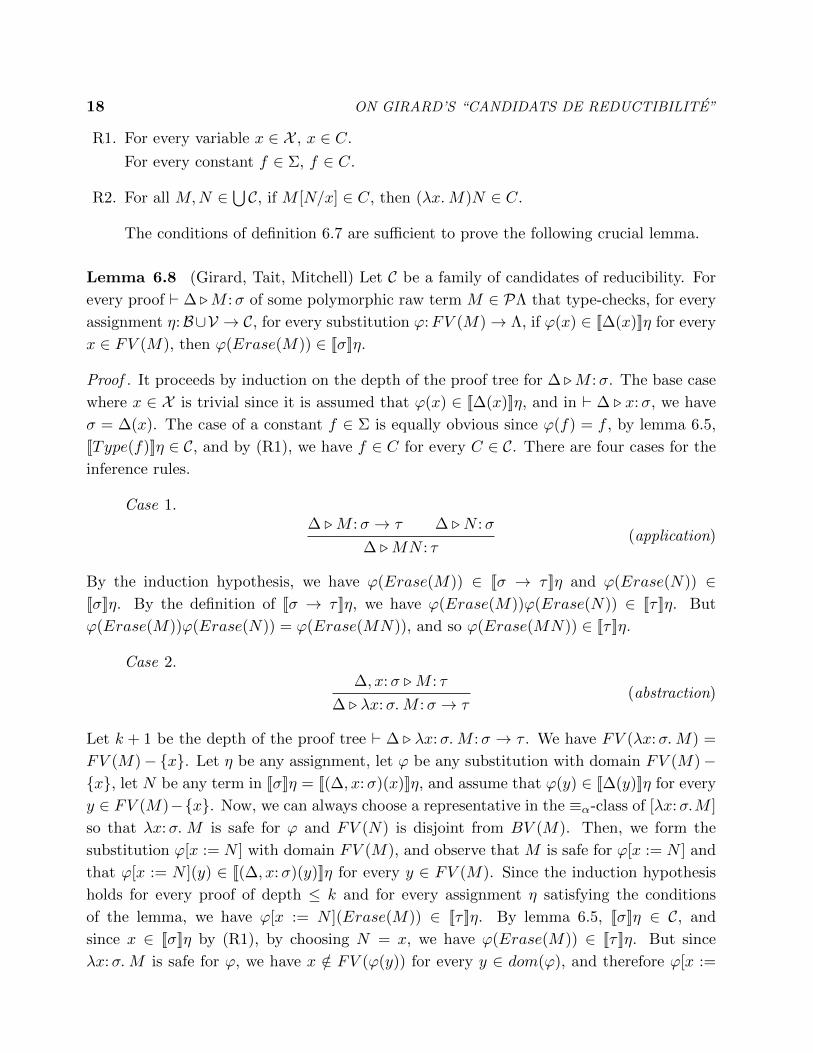
R1. For every variable x 2 X , x 2 C.
For every constant f 2 ⌃, f 2 C.
R2. For all M,N 2S
C, if M [N/x] 2 C, then (�x. M)N 2 C.
The conditions of definition 6.7 are su�cient to prove the following crucial lemma.
Lemma 6.8 (Girard, Tait, Mitchell) Let C be a family of candidates of reducibility. For
every proof ` � .M :� of some polymorphic raw term M 2 P⇤ that type-checks, for every
assignment ⌘:B[V ! C, for every substitution ':FV (M)! ⇤, if '(x) 2 [[�(x)]]⌘ for every
x 2 FV (M), then '(Erase(M)) 2 [[�]]⌘.
Proof . It proceeds by induction on the depth of the proof tree for � .M :�. The base case
where x 2 X is trivial since it is assumed that '(x) 2 [[�(x)]]⌘, and in ` � . x:�, we have
� = �(x). The case of a constant f 2 ⌃ is equally obvious since '(f) = f , by lemma 6.5,
[[Type(f)]]⌘ 2 C, and by (R1), we have f 2 C for every C 2 C. There are four cases for the
inference rules.
Case 1.� .M :� ! ⌧ � .N :�
� .MN : ⌧(application)
By the induction hypothesis, we have '(Erase(M)) 2 [[� ! ⌧ ]]⌘ and '(Erase(N)) 2[[�]]⌘. By the definition of [[� ! ⌧ ]]⌘, we have '(Erase(M))'(Erase(N)) 2 [[⌧ ]]⌘. But
'(Erase(M))'(Erase(N)) = '(Erase(MN)), and so '(Erase(MN)) 2 [[⌧ ]]⌘.
Case 2.�, x:� .M : ⌧
� . �x:�. M :� ! ⌧(abstraction)
Let k + 1 be the depth of the proof tree ` � . �x:�. M :� ! ⌧ . We have FV (�x:�. M) =
FV (M)� {x}. Let ⌘ be any assignment, let ' be any substitution with domain FV (M)�{x}, let N be any term in [[�]]⌘ = [[(�, x:�)(x)]]⌘, and assume that '(y) 2 [[�(y)]]⌘ for every
y 2 FV (M)�{x}. Now, we can always choose a representative in the ⌘↵
-class of [�x:�.M ]
so that �x:�. M is safe for ' and FV (N) is disjoint from BV (M). Then, we form the
substitution '[x := N ] with domain FV (M), and observe that M is safe for '[x := N ] and
that '[x := N ](y) 2 [[(�, x:�)(y)]]⌘ for every y 2 FV (M). Since the induction hypothesis
holds for every proof of depth k and for every assignment ⌘ satisfying the conditions
of the lemma, we have '[x := N ](Erase(M)) 2 [[⌧ ]]⌘. By lemma 6.5, [[�]]⌘ 2 C, and
since x 2 [[�]]⌘ by (R1), by choosing N = x, we have '(Erase(M)) 2 [[⌧ ]]⌘. But since
�x:�. M is safe for ', we have x /2 FV ('(y)) for every y 2 dom('), and therefore '[x :=

6 An Untyped Version of The Candidates of Reducibility 19
N ](Erase(M)) = '(Erase(M))[N/x].6 Thus, '(Erase(M))[N/x] 2 [[⌧ ]]⌘. Since N 2 [[�]]⌘
and '(Erase(M)) 2 [[⌧ ]]⌘, by lemma 6.5, we have N 2S
C and '(Erase(M)) 2S
C. Thus,we can apply (R2) to '(Erase(M))[N/x] 2 [[⌧ ]]⌘, and we have (�x.'(Erase(M)))N 2 [[⌧ ]]⌘.
It is easily verified that �x.'(Erase(M)) = '(Erase(�x:�.M)) (using the fact that �x:�.M
is safe for '). Since '(Erase(�x:�.M))N 2 [[⌧ ]]⌘ holds for every N 2 [[�]]⌘, by the definition
of [[� ! ⌧ ]]⌘, we have '(Erase(�x:�. M)) 2 [[� ! ⌧ ]]⌘.7
Case 3.� .M : 8t. �
� .M⌧ :�[⌧/t](type application)
By the induction hypothesis, '(Erase(M)) 2 [[8t. �]]⌘. Since [[8t. �]]⌘ =T
C2C [[�]]⌘[t := C],
we have '(Erase(M)) 2 [[�]]⌘[t := C] for every C 2 C. Since by lemma 6.5, [[⌧ ]]⌘ 2 C,by setting C = [[⌧ ]]⌘, we have '(Erase(M)) 2 [[�]]⌘[t := [[⌧ ]]⌘]. However, by lemma 6.6,
[[�[⌧/t]]]⌘ = [[�]]⌘[t := [[⌧ ]]⌘], and so '(Erase(M⌧)) = '(Erase(M)) 2 [[�[⌧/t]]]⌘.
Case 4.� .M :�
� . ⇤t. M : 8t. �(type abstraction)
where in this rule, t /2 FV(�(x)) for every x 2 dom(�) \ FV (M).
Let k + 1 be the depth of the proof tree for � . ⇤t. M : 8t. �. Since t /2 FV(�(x)) for
every x 2 dom(�) \ FV (M), by lemma 6.4, we have [[�(x)]]⌘ = [[�(x)]]⌘[t := C] for every
C 2 C. Since the induction hypothesis holds for every proof tree of depth k, for every ⌘,
and for every ' satisfying the conditions of the lemma, it holds for every C 2 C when applied
to the proof tree ` � .M :�, to every ⌘[t := C], and to every ' such that '(x) 2 [[�(x)]]⌘
for every x 2 FV (M).8 Thus, '(Erase(M)) 2 [[�]]⌘[t := C] for every C 2 C, that is,
'(Erase(⇤t. M)) = '(Erase(M)) 2 [[8t. �]]⌘, since [[8t. �]]⌘ =T
C2C [[�]]⌘[t := C].
Remark : It should be observed that lemma 6.8 still holds if condition (R2) of definition
6.7 is changed to:
R20. For all M,N 2 ⇤, if M [N/x] 2 C, then (�x. M)N 2 C.
6 This subtle point seems to have been overlooked in all proofs that we have read, including Girard’soriginal proof(s). The problem is that '[x := N ](Erase(M)) = '(Erase(M))[N/x] may be false ifx appears in '(y) for some y 2 dom(')!
7 Observe that this step of the proof is possible because we can apply the induction hypothesis toevery substitution of the form '[x := N ] where N is any term in [[�]]⌘. This is why we need theuniversal quantification on the substitution ' in the statement of the lemma. Without it, the proofwould not go through.
8 Observe that this step of the proof is possible because we can apply the induction hypothesis toevery assignment of the form ⌘[t := C] where C is any set in C. This is why we need the universalquantification on the assignment ⌘ in the statement of the lemma. Without it, the proof would notgo through.

20 ON GIRARD’S “CANDIDATS DE REDUCTIBILITE”
The di↵erence between (R2) and (R20) is that in (R2)M and N belong toS
C, whereasin (R20), M and N are arbitrary terms. Our motivation for using (R2) is that one can take
advantage of the fact that M,N 2S
C in establishing (R2).
By choosing ' to be the identity, lemma 6.8 implies that Erase(M) 2 [[�]]⌘ for every
term that type-checks. Thus, in order to prove properties of terms of the form Erase(M)
where M type-checks, one needs to know how to generate families of candidates of reducibil-
ity satisfying some given properties. For this, it appears that it is necessary to strengthen
conditions (R1) and (R2). Girard provided su�cient conditions (Girard [9], Girard [10]).
Here, we give some slightly more general conditions adapted from Mitchell ([24]) and Tait
([37]).
Definition 6.9 Let S be a nonempty set of (untyped) lambda terms. We say that S is
closed i↵ whenever Mx 2 S where x 2 X , then M 2 S. A subset C ✓ S is saturated i↵ the
following conditions hold:9
S1. For every variable x 2 X , for all n � 0 and all N1, . . . , Nn
2 S, xN1 . . . Nn
2 C.
For every constant f 2 ⌃, for all n � 0 and all N1, . . . , Nn
2 S, fN1 . . . Nn
2 C.
S2. For all M,N 2 S, for all n � 0 and all N1, . . . , Nn
2 S, if M [N/x]N1 . . . Nn
2 C, then
(�x. M)NN1 . . . Nn
2 C.
The following result shows the significance of saturated subsets of a closed set of
lambda terms.
Lemma 6.10 (Girard, Tait, Mitchell) Let S be a nonempty closed set of (untyped) lambda
terms, let C be the family of all saturated subsets of S, and assume that S 2 C (i.e. S is a
saturated subset of itself). Then C is a family of candidates of reducibility.
Proof . Since S 2 C, C is nonempty. Clearly, by condition (S1) of saturated sets in the case
n = 0, each saturated set is nonempty. Let C and D be any two saturated subsets of S.
Recall that [C ! D] = {M | 8N 2 C, MN 2 D}. We need to show that [C ! D] is a
saturated subset of S.
For every M 2 [C ! D], by (S1), since there is some variable x 2 C, Mx 2 D, and
since S is closed, we have M 2 S. Thus [C ! D] is a subset of S.
Since D is saturated, by (S1) for every variable x 2 X and for all m � 0 and all
N1, . . . , Nm
, N 2 S, we have xN1 . . . Nm
N 2 D. Since this holds for every N 2 C, we have
9 We also have to assume that every saturated subset of S is closed under ↵-equivalence.
6 An Untyped Version of The Candidates of Reducibility 21
xN1 . . . Nn
2 [C ! D].10 The second case of (S1) for a constant in ⌃ is similar. Thus, (S1)
holds for [C ! D].
For every N 2 S, all m � 0, all N1, . . . , Nm
2 S, assume that M [N/x]N1 . . . Nm
2[C ! D]. This means that for every P 2 C, M [N/x]N1 . . . Nm
P 2 D. Since D is saturated,
by (S2), (�x. M)NN1 . . . Nm
P 2 D, and since this is true for every P 2 C, we have
(�x. M)NN1 . . . Nm
2 [C ! D].11 This shows that (S2) holds for [C ! D].
Finally, it is clear that properties (S1) and (S2) of saturated subsets of S are closed
under arbitrary intersections, and so for any C-indexed family (AC
)C2C of saturated subsets
of S,T
C2C AC
is also a saturated subset of S.
Remark . Besides implying (R1) and (R2) respectively, conditions (S1) and (S2) ensure
that [C ! D] also satisfies (S1) and (S2) if C and D do. It should be noted that if we are
interested in the version of the candidates in which condition (R20) is used, then lemma
6.10 holds if the clause M,N,N1, . . . , Nn
2 S in condition (S2) of definition 6.9 is changed
to N 2 S, M,N1, . . . , Nn
2 ⇤, obtaining the condition (S20). Conditions (S1) and (S20) are
essentially Mitchell’s conditions [24].
It is interesting to note that the reason why lemma 6.10 holds is that (S1) and (S2)
have certain “right-invariant” properties.
Definition 6.11 Define a predicate � on ⇤ to be right-invariant i↵ for every M,N 2 ⇤, if
�(M) then �(MN). Let S� = {M 2 ⇤ | �(M)}. A binary relation ⇢ on ⇤ is right-invariant
i↵ for every M1,M2, N 2 ⇤, if ⇢(M1,M2) then ⇢(M1N,M2N). A set C ✓ ⇤ is closed under
⇢ i↵ for every M,N 2 ⇤, if M 2 C and ⇢(M,N), then N 2 C.
Lemma 6.12 If S� ✓ C for every set in a family C and � is right-invariant, then S�
is also a subset of every set of the form [C ! D] with C,D 2 C, and a subset of every
intersectionT
C2C AC
.
Proof . Let M be any term in ⇤. We have to show that if �(M) holds then M 2 [C ! D].
Since � is right-invariant, for every N 2 C we have �(MN). Since S� ✓ D, we have
MN 2 D. This shows that M 2 [C ! D]. Obviously, S� is also a subset of every
intersectionT
C2C AC
.
Lemma 6.13 If ⇢ is right-invariant and every set in a family C is closed under ⇢, then
every set of the form [C ! D] with C,D 2 C is closed under ⇢ and every intersectionTC2C AC
is closed under ⇢.
10 Note how we have used the fact that (S1) holds for all n � 0, and applied (S1) with n = m + 1 forany arbitrary m. The proof would not go through if (S1) was assumed only for n = 0.
11 Again, note how we have used the fact that (S2) holds for all n � 0.

22 ON GIRARD’S “CANDIDATS DE REDUCTIBILITE”
Proof . If M1 2 [C ! D], M2 2 ⇤ and ⇢(M1,M2), by right-invariance ⇢(M1N,M2N) for
every N 2 C. Since M1N 2 D and D is closed under ⇢, we have M2N 2 D. But this shows
that M2 2 [C ! D], i.e., [C ! D] is closed under ⇢. It is obvious that every intersectionTC2C AC
is closed under ⇢.
Lemma 6.12 can be applied to � defined such that for every M 2 ⇤, �(M) i↵ 9u 2X[⌃, 9N1, . . . , Nm
2 ⇤, M = uN1 . . . Nm
. In this case � corresponds to (S1). Lemma 6.13
can be applied to ⇢ defined such that ⇢(M1,M2) i↵ 9M,N 2 ⇤, 9N1, . . . , Nm
2 ⇤, M1 =
M [N/x]N1 . . . Nm
, and M2 = (�x. M)NN1 . . . Nm
. In this case ⇢ corresponds to (S2).
Thus, it seems that the way to obtain the conditions (Si) from the conditions (Ri) is
to make the (Ri) right-invariant. Indeed, this is the way to handle other type constructors,
such as products and existential types. We have the following lemma generalizing lemma
6.10.
Lemma 6.14 Let S be a nonempty closed set of (untyped) lambda terms, let F� be a
family of right-invariant predicates on ⇤, and F⇢
a family of right-invariant binary relations
on ⇤. Let C be the family of all subsets C of S such that:
(1) S� ✓ C, for every � 2 F�;
(2) C is closed under ⇢, for every ⇢ 2 F⇢
.
Then C is closed under the function space constructor and under intersections of the
formT
C2C AC
.
Proof . Similar to lemma 6.10, using lemma 6.12 and lemma 6.13.
After this short digression, we state the fundamental result about the method of
candidates.
Theorem 6.15 (Girard, Tait, Mitchell) Let S be a nonempty closed set of (untyped)
lambda terms, let C be the family of all saturated subsets of S, and assume that S 2 C(i.e. S is a saturated subset of itself). For every polymorphic raw term M 2 P⇤, if M
type-checks, then Erase(M) 2 S.
Proof . By lemma 6.10, C is a family of candidates of reducibility. We now apply lemma 6.8
to any assignment (for example, the constant assignment with value S) and to the identity
substitution, which is legitimate since by (S1), every variable belongs to every saturated
set.12
12 Actually, given any term M , we may need to perform some ↵-renaming on M to get an M
0 such thatM
0 is safe for the identity substitution. Lemma 6.8 then yields the fact that Erase(M 0) 2 S. But S
is closed under ⌘↵, and so Erase(M) 2 S.

6 An Untyped Version of The Candidates of Reducibility 23
Thus, in order to apply theorem 6.15, one needs to have useful examples of closed sets
S that are saturated. This is the purpose of the next lemma.
Lemma 6.16 (Girard, Tait, Mitchell) (i) The set SN�
of (untyped) lambda terms that
are strongly normalizing under �-reduction is a closed saturated set. (ii) The set SN�⌘
of (untyped) lambda terms that are strongly normalizing under �⌘-reduction is a closed
saturated set. (iii) The set of lambda terms M such that confluence holds under �-reduction
from M and all of its subterms is a closed saturated set. (iv) The set of lambda terms M
such that confluence holds under �⌘-reduction from M and all of its subterms is a closed
saturated set.
Proof . (i)-(ii) Verifying closure is easy: if Mx is SN, then M must be SN, since other-
wise an infinite reduction sequence from M would yield an infinite reduction from Mx.
Verifying (S1) is also straightforward, since the existence of an infinite reduction sequence
from uN1 . . . Nm
implies that there is some infinite reduction sequence from some Ni
, con-
tradicting the assumption that each Ni
is SN. Verifying (S2) is a little harder. We prove
that if N is SN and there is an infinite reduction sequence from (�x. M)NN1 . . . Nm
, then
there is an infinite reduction sequence from M [N/x]N1 . . . Nm
.13 The proof is slightly more
complicated in the case of �⌘-reduction than it is in the case of �-reduction alone, because
of possible head ⌘-reductions.
Consider any infinite reduction sequence from (�x. M)NN1 . . . Nm
. There are three
di↵erent possible patterns:
(1) every term in this sequence is of the form (�x. M 0)N 0N 01 . . . N
0m
, where M⇤�!
�
M 0,
N⇤�!
�
N 0, and Ni
⇤�!�
N 0i
for i = 1, . . . ,m, or
(2) there is a step (�x. M 0)N 0N 01 . . . N
0m
�!�
M 0[N 0/x]N 01 . . . N
0m
in this sequence, for
some M 0, N 0, N 01, . . . , N
0m
, such that M⇤�!
�
M 0, N⇤�!
�
N 0, and Ni
⇤�!�
N 0i
for
i = 1, . . . ,m, or
(3) M⇤�!
�
M 01x, and there is a step
(�x. (M 01x))N
0N 01 . . . N
0m
�!⌘
M 01N
0N 01 . . . N
0m
,
for some N 0, N 01, . . . , N
0m
, such that N⇤�!
�
N 0, and Ni
⇤�!�
N 0i
, for i = 1, . . . ,m.
In case (1), it is clear that the given infinite reduction sequence defines uniquely
some independent finite or infinite reduction sequences originating from each of M , N ,
N1, . . . , Nm
. Since N is assumed to be SN, one of the sequences originating from M ,
13 This proof is inspired by Tait [37].

24 ON GIRARD’S “CANDIDATS DE REDUCTIBILITE”
N1, . . . , Nm
must be infinite, and by lemma 5.7, we obtain an infinite reduction sequence
from M [N/x]N1 . . . Nm
.
In case (2), there are some terms M 0, N 0, N 01, . . . , N
0m
, such that M⇤�!
�
M 0,
N⇤�!
�
N 0, and Ni
⇤�!�
N 0i
for i = 1, . . . ,m, and M 0[N 0/x]N 01 . . . N
0m
is the head of
some infinite reduction sequence ⇡. Using lemma 5.7, we can form the reduction sequence
(�x. M)NN1 . . . Nm
�!�
M [N/x]N1 . . . Nm
⇤�!�
M 0[N 0/x]N 01 . . . N
0m
,
which can be extended to an infinite reduction sequence using ⇡.
In case (3), since M⇤�!
�
M 01x, using lemma 5.7, we have a reduction
(�x. M)NN1 . . . Nm
�!�
M [N/x]N1 . . . Nm
⇤�!�
M 01[N/x]N 0N 0
1 . . . N0m
.
However, because in (3) we have an ⌘-reduction step, x /2 FV (M 01), and so M 0
1[N/x] = M 01.
Thus, M 01[N/x]N 0N 0
1 . . . N0m
= M 01N
0N 01 . . . N
0m
. Since there is an infinite reduction from
M 01N
0N 01 . . . N
0m
, we have an infinite reduction from M [N/x]N1 . . . Nm
.
(iii)-(iv) The proof will be given in section 7 for the typed case.
We can apply theorem 6.15 to the set SN�⌘
, which, by lemma 6.16, is closed and
saturated, and we obtain the following corollary to theorem 6.15.
Lemma 6.17 For every polymorphic raw term M , if M type-checks then Erase(M) is
strongly normalizable under �⌘-reduction.
Using lemma 5.6, we have:
Lemma 6.18 Every polymorphic raw term M that type-checks is strongly normalizable
under �⌘-reduction.
Applying theorem 6.15 to the set of terms M such that confluence holds (under �-
reduction or �⌘-reduction) from M and all of its subterms, which, by lemma 6.16, is closed
and saturated, we have:
Lemma 6.19 (Mitchell) The reduction relation �!�
(�⌘-reduction) is confluent on terms
of the form Erase(M), where M type-checks. The result also holds for �-reduction.
Unfortunately, we have not been unable to show that lemma 6.19 implies that �!�
8
is confluent on polymorphic terms that type-check. However, this result can be established
using a typed version of the candidates of reducibility.

7 A Typed Version of The Candidates of Reducibility 25
7 A Typed Version of The Candidates of Reducibility
We now describe a typed version of the “candidats de reductibilite”, as originally defined
by Girard (Girard 1970 [9], Girard 1972 [10]). We will present two sets of conditions for the
typed candidates. The first set consists of conditions similar to those used by Stenlund [35],
(basically the typed version of Tait’s conditions, Tait 1973 [37]), and the second set consists
of Girard’s original conditions (Girard [10], [11]). We also compare these conditions, and
prove that Girard’s conditions are stronger than Tait’s conditions.
Rather than using explicitly typed polymorphic terms as in Girard [10], we work with
provable typing judgments.
Definition 7.1 For every type �, let PT�
be the set of all provable typing judgments of
type � (the provable typing judgments of the form � .M :� for arbitrary � and M).
In order to reduce the amount of notation, if S is a set of provable typing judgments
of type �, rather than writing � .M :� 2 S, we will write � .M 2 S.
Given any two types �, ⌧ 2 T and any two sets S ✓ PT�
and T ✓ PT⌧
, we let
[S ! T ] be the subset of PT�!⌧
defined as follows:
[S ! T ] = {� .M 2 PT�!⌧
| 8�0 .N, if � ✓ �0 and �0 .N 2 S, then �0 .MN 2 T}.
We also refer to the operation ! on sets of provable typing judgments defined above as the
function space constructor .
Definition 7.2 Let C = (C�
)�2T be a T -indexed family where each C
�
is a nonempty set
of subsets of PT�
, and the following properties hold:
(1) For every � 2 T , every C 2 C�
is a nonempty subset of PT�
.
(2) For every �, ⌧ 2 T , for every C 2 C�
and every D 2 C⌧
, we have [C ! D] 2 C�!⌧
.
(3) For every 8t. �, ⌧ 2 T , for every family (A⌧,C
)⌧2T ,C2C⌧ , where each set A
⌧,C
is in
C�[⌧/t], we have
{� .M 2 PT 8t. � | 8⌧ 2 T , � .M⌧ 2\
C2C⌧
A⌧,C
} 2 C8t. �.
A family satisfying the above conditions is called a T -closed family .

26 ON GIRARD’S “CANDIDATS DE REDUCTIBILITE”
Definition 7.3 Let C be a T -closed family. A pair h✓, ⌘i where ✓:V ! T is a type
substitution and ⌘:B [ V !S
C is a candidate assignment i↵ ⌘(t) 2 C✓(t) for every t 2 V
and ⌘(�) 2 C�
for every � 2 B.
We can associate certain sets of provable typing judgments to the types inductively
as explained below.
Definition 7.4 Given any candidate assignment h✓, ⌘i, for every type �, the set [[�]]✓⌘ is
a subset of PT✓(�) defined as follows:
[[t]]✓⌘ = ⌘(t), whenever t 2 B [ V,[[(� ! ⌧)]]✓⌘ = [[[�]]✓⌘ ! [[⌧ ]]✓⌘],
[[8t. �]]✓⌘ = {� .M 2 PT✓(8t. �) | 8⌧ 2 T ,
� .M⌧ 2\
C2C⌧
[[�]]✓[t := ⌧ ]⌘[t := C]}.
Strictly speaking, [[�]]✓⌘ is defined for the ⌘↵
-class [�] of �. Thus, it can be assumed
that � is safe for ✓. For a type 8t. �, this implies that t /2 FV(✓(v)) for every v 2 dom(✓),
and consequently that ✓[t := ⌧ ](�) = ✓(�)[⌧/t]. This shows that the sets of terms involved
in the intersection are indeed of the right type ✓(�)[⌧/t].
The following technical lemma will be useful later.
Lemma 7.5 Given any two candidate assignments h✓1, ⌘1i and h✓2, ⌘2i, for every type �,
if ✓1, ✓2 agree on FV(�), and ⌘1, ⌘2 agree on FV(�) and B, then [[�]]✓1⌘1 = [[�]]✓2⌘2.
Proof . Easy induction on the structure of types.
We now have a typed version of “Girard’s trick”.
Lemma 7.6 (Girard) If C is a T -closed family, for every candidate assignment h✓, ⌘i, forevery type �, then [[�]]✓⌘ 2 C
✓(�).
Proof . The lemma is proved by induction on the structure of types. The proof is similar
to the proof of lemma 6.5. The only case worth mentioning is the case of a universal
type. Given a type 8t. � and a candidate assignment h✓, ⌘i, using ↵-renaming, it can be
assumed that 8t. � is safe for ✓. By the induction hypothesis, [[�]]✓⌘ 2 C✓(�). Thus, for
every ⌧ 2 T and for every C 2 C✓[t:=⌧ ](�), we also have [[�]]✓[t := ⌧ ]⌘[t := C] 2 C
✓[t:=⌧ ](�).
However, ✓[t := ⌧ ](�) = ✓(�)[⌧/t] as we observed earlier since 8t. � is safe for ✓. Thus,
[[�]]✓[t := ⌧ ]⌘[t := C] 2 C✓(�)[⌧/t], and we conclude by condition (3) of T -closed families.
The following technical lemma will be needed later.

7 A Typed Version of The Candidates of Reducibility 27
Lemma 7.7 Given any two types �, ⌧ , for every candidate assignment h✓, ⌘i,
[[�[⌧/t]]]✓⌘ = [[�]]✓[t := ✓(⌧)]⌘[t := [[⌧ ]]✓⌘].
Proof . Straightforward induction on the structure of �.
In order to use lemma 7.6 in proving properties of polymorphic lambda calculi, we
need to define T -closed families satisfying some additional properties.
Definition 7.8 We say that a T -indexed family C is a family of sets of candidates of
reducibility i↵ it is T -closed and satisfies the conditions listed below:14
R0. Whenever � .M 2 C and � ✓ �0, then �0 .M 2 C.
R1. For every � 2 T , for every set C 2 C�
, � . x 2 C, for every x:� 2 �,
For every � = Type(f), for every set C 2 C�
, � . f 2 C, for every f 2 ⌃.
R2. (i) For all �, ⌧ 2 T , for every C 2 C⌧
, for all �,�0, if
� .M 2[
C⌧
,
�0 .N 2[
C�
, and
�0 .M [N/x] 2 C, then
�0 . (�x:�. M)N 2 C.
(ii) For all �, ⌧ 2 T , for every C 2 C�[⌧/t], if
� .M 2[
C�
and
� .M [⌧/t] 2 C, then
� . (⇤t. M)⌧ 2 C.
As in the untyped case, (R0), (R1), and (R2), are all we need to prove the following
fundamental result.
Lemma 7.9 (Girard) Let C = (C�
)�2T be a T -indexed family of sets of candidates of
reducibility. For every � . M 2 PT�
, for every candidate assignment h✓, ⌘i, for every
substitution ':� ! �, if ✓(�) . '(x) 2 [[�(x)]]✓⌘ for x 2 FV (M), then ✓(�) . '(✓(M)) 2[[�]]✓⌘.
Proof . It is similar to the proof of lemma 6.8 and proceeds by induction on the depth of
the proof tree for � .M :�. The only cases worth considering are type abstraction and type
14 Again, we also have to assume that every C 2 C is closed under ↵-equivalence.

28 ON GIRARD’S “CANDIDATS DE REDUCTIBILITE”
application, the other two being essentially unchanged, except that (R0) is needed in the
case of �-abstraction.
Case 3.� .M : 8t. �
� .M⌧ :�[⌧/t](type application)
First, by suitable ↵-renaming, it can be assumed that M⌧ is safe for ' and ✓, and that 8t.�is safe for ✓. By the induction hypothesis, ✓(�) . '(✓(M)) 2 [[8t. �]]✓⌘. By the definition of
[[8t. �]]✓⌘, we have
✓(�) . '(✓(M))� 2 [[�]]✓[t := �]⌘[t := C],
for every � 2 T and C 2 C�
. Since 8t.� is safe for ✓, as observed before, we have ✓(�)[�/t] =
✓[t := �](�). Since by lemma 7.6, [[⌧ ]]✓⌘ 2 C✓(⌧), by setting � = ✓(⌧) and C = [[⌧ ]]✓⌘, we have
✓(�) . '(✓(M))✓(⌧) 2 [[�]]✓[t := ✓(⌧)]⌘[t := [[⌧ ]]✓⌘].
Since 8t.� is safe for ✓ and ' and ✓ have disjoint domains, we have '(✓(M))✓(⌧) = '(✓(M⌧))
and ✓(�)[✓(⌧)/t] = ✓(�[⌧/t]), and so
✓(�) . '(✓(M⌧)) 2 [[�]]✓[t := ✓(⌧)]⌘[t := [[⌧ ]]✓⌘].
However, by lemma 7.7, [[�[⌧/t]]]✓⌘ = [[�]]✓[t := ✓(⌧)]⌘[t := [[⌧ ]]✓⌘], and so
✓(�) . '(✓(M⌧)) 2 [[�[⌧/t]]]✓⌘.
Case 4.� .M :�
� . ⇤t. M : 8t. �(type abstraction)
where in this rule, t /2 FV(�(x)) for every x 2 dom(�) \ FV (M).
Let k + 1 be the depth of the proof tree for � . ⇤t. M : 8t. �. Since t /2 FV(�(x)) forevery x 2 dom(�) \ FV (M), by lemma 7.5, we have [[�(x)]]✓⌘ = [[�(x)]]✓[t := ⌧ ]⌘[t := C],
for every ⌧ 2 T and every C 2 C⌧
. By the induction hypothesis,
✓(�) . '(✓[t := ⌧ ](M)) 2 [[�]]✓[t := ⌧ ]⌘[t := C],
for every ⌧ 2 T and every C 2 C⌧
. By suitable ↵-renaming, it can be assumed that
⇤t. M is safe for ' and ✓, that 8t. � is safe for ✓, and that t /2 FV(�(x)) for every
x 2 dom(�). Then, ✓[t := ⌧ ](�) = ✓(�), and as observed before, ✓[t := ⌧ ](M) = ✓(M)[⌧/t],
✓[t := ⌧ ](�) = ✓(�)[⌧/t], and since ' and ✓[t := ⌧ ] have disjoint domains, we have
✓(�) . '(✓(M))[⌧/t] 2 [[�]]✓[t := ⌧ ]⌘[t := C],

8 Families of Sets of Saturated Sets 29
for every ⌧ 2 T and every C 2 C⌧
. In particular, since t 2 T , by choosing ⌧ = t, we
have ✓(�) . '(✓(M)) 2 [[�]]✓⌘[t := C]. Since by lemma 7.6, [[�]]✓⌘[t := C] 2 C✓(�), we have
'(✓(M)) 2S
C✓(�). Thus, by (R2)(ii), we have
✓(�) . (⇤t. '(✓(M)))⌧ 2 [[�]]✓[t := ⌧ ]⌘[t := C],
that is
✓(�) . '(✓(⇤t. M))⌧ 2 [[�]]✓[t := ⌧ ]⌘[t := C],
for every ⌧ 2 T and every C 2 C⌧
. By definition 7.4, this means that
✓(�) . '(✓(⇤t. M)) 2 [[8t. �]]✓⌘.
Remark : As in the remark just after lemma 6.8, it should be observed that lemma 7.9
still holds if condition (R2) of definition 7.8 is relaxed so that in (R2)(i),S
C⌧
is replaced
by PT⌧
,SC�
by PT�
, and in (R2)(ii),S
C�
is replaced by PT�
. The relaxed conditions
will be called (R20)(i) and and (R20)(ii).
In order to prove that families of sets of candidates of reducibility exist, one needs
conditions stronger that (R1) and (R2). First, we give conditions adapted from Tait and
Mitchell.
8 Families of Sets of Saturated Sets
The definition of the saturated sets given in the untyped case (definition 6.9) is adapted as
follows.
Definition 8.1 Let S = (S�
)�2T be a T -indexed family such that each S
�
is a nonempty
subset of PT�
. We say that S is closed i↵ for all �, ⌧ 2 T , for every x 2 X , if�.M 2 PT�!⌧
and �, x:� .Mx 2 S⌧
, then � .M 2 S�!⌧
, and for every t 2 V, if � .M 2 PT 8t. � and
� .Mt 2 S�
, then � .M 2 S8t. �. The family Sat(S) = (Sat(S)�
)�2T of sets of saturated
subsets of S is defined such that for every � 2 T , Sat(S)�
consists of those subsets C ✓ S�
such that the following conditions hold:15
S0. Whenever � .M 2 C and � ✓ �0, then �0 .M 2 C.
15 We also have to assume that every saturated subset of S is closed under ↵-equivalence.

30 ON GIRARD’S “CANDIDATS DE REDUCTIBILITE”
S1. For every type � 2 T , for every C 2 Sat(S)�
, for all n � 0, for allN1, . . . , Nn
2 T [P⇤,
for every u 2 X [ ⌃, if
� . uN1 . . . Nn
2 PT�
, and
� .Ni
2 S⇠i for some ⇠
i
whenever Ni
is a term (1 i n), then
� . uN1 . . . Nn
2 C.
S2. (i) For all �, ⌧ 2 T , for every C 2 Sat(S)⌧
, for all n � 0, for all N1, . . . , Nn
2 T [P⇤,
for all �,�0, if
� .M 2 S⇠
for some ⇠,
�0 .M [N/x]N1 . . . Nn
2 C,
�0 .N 2 S�
, and
�0 .Ni
2 S⇠i for some ⇠
i
whenever Ni
is a term (1 i n), then
�0 . (�x:�. M)NN1 . . . Nn
2 C.
(ii) For all �, ⌧ 2 T , for every C 2 Sat(S)�
, for all n � 0, for all N1, . . . , Nn
2 T [P⇤,
if
� .M [⌧/t]N1 . . . Nn
2 C,
� .M 2 S⇠
for some ⇠, and
� .Ni
2 S⇠i for some ⇠
i
whenever Ni
is a term (1 i n), then
� . (⇤t. M)⌧N1 . . . Nn
2 C.
We have the following typed version of lemma 6.10.
Lemma 8.2 (Girard, Tait, Mitchell) Let S = (S�
)�2T be a closed family where each S
�
is a nonempty subset of PT�
, let C be the T -indexed family of sets of saturated subsets of
S, and assume that S�
2 C�
for every � 2 T (i.e. S�
is a saturated subset of itself). Then
C is a family of sets of candidates of reducibility.
Proof . It is similar to the proof of lemma 6.10. One point worth mentioning is the necessity
of allowingN1 . . . Nn
to be terms or types, in order to prove closure condition (3) of definition
7.2.
We now consider the conditions used by Girard in [10] and [11], and their relationship
to Tait and Mitchell’s conditions.
9 Families of Sets of Girard Sets 31
9 Families of Sets of Girard Sets
Girard’s conditions basically assert that complete induction holds for certain simple terms
w.r.t. �!�
8 .
Definition 9.1 A simple term is a term that is not an abstraction. Thus, a term M
is simple i↵ it is either a variable x, a constant f 2 ⌃, an application MN , or a type
application M⌧ .
The idea behind this definition is that for a simple term M , for every term N , if
MN �!�
8 Q, then either M �!�
8 M 0 and Q = M 0N , or N �!�
8 N 0 and Q = MN 0.
Definition 9.2 Let S = (S�
)�2T be a T -indexed family such that each S
�
is a nonempty
subset of PT�
. A subset C of S�
is a Girard set of type � i↵ the following conditions hold:16
CR0. Whenever � .M 2 C and � ✓ �0, then �0 .M 2 C.
CR1. If � .M 2 C, then M is SN w.r.t �!�
8 ;
CR2. If � .M 2 C and M �!�
8 N , then � .N 2 C;
CR3. For every simple term �.M 2 PT�
, if �.N 2 C for every N such that M �!�
8 N ,
then � .M 2 C.
Note that (CR3) implies that all simple irreducible terms are in C. We shall prove a
lemma analogous to lemma 8.2 for families of sets of Girard subsets, but first, we establish
a precise connection between Girard sets and saturated sets. We prove that conditions
(CR1), (CR2) and (CR3) imply conditions (S1) and (S2).
Lemma 9.3 Let S = (S�
)�2T be a family where each S
�
is a Girard subset of PT�
.
Every Girard subset of S is a saturated set, i.e., satisfies conditions (S1), (S2).
Proof . We first make the following observation. For every term M , it is clear that there are
only finitely many terms N such that M �!�
8 N . Thus, for every SN term M , by Konig’s
lemma, the tree of reduction sequences from M is finite. Thus, for every SN term M , the
depth of the reduction tree from M is well defined, and we denote it as �(M).
We now prove (S1). For every u 2 X [ ⌃, assume that
� . uN1 . . . Nn
2 PT�
, and
� .Ni
2 S⇠i for some ⇠
i
whenever Ni
is a term (1 i n).
16 We also have to assume that every Girard subset of S is closed under ↵-equivalence.

32 ON GIRARD’S “CANDIDATS DE REDUCTIBILITE”
We prove by complete induction on � = �(N1)+ . . .+ �(Nn
) that �.uN1 . . . Nn
2 C. Since
uN1 . . . Nn
is a simple term, we can do this by using (CR3).
The base case � = 0 holds, since then uN1 . . . Nn
is simple and irreducible. For the
induction step, note that uN1 . . . Nn
�!�
8 Q implies that Q = uN1 . . . N0i
. . . Nn
, where
Ni
�!�
8 N 0i
. Also, ifNi
�!�
8 N 0i
, by (CR2) we have�.N 0i
2 S⇠i , and since �(N 0
i
) < �(Ni
),
the induction hypothesis implies that � .uN1 . . . N0i
. . . Nn
2 C. Using (CR3), we conclude
that � . uN1 . . . Nn
2 C.
We also prove (S2). Assume that for some �,�0,
� .M 2 S⇠
for some ⇠,
�0 .M [N/x]N1 . . . Nn
2 C,
�0 .N 2 S�
, and
�0 .Ni
2 S⇠i for some ⇠
i
whenever Ni
is a term (1 i n).
We want to prove that �0 . (�x:�. M)NN1 . . . Nn
2 C. Since (�x:�. M)NN1 . . . Nn
is
a simple term, we can do this by using (CR3). Since the terms M,N,N1, . . . , Nn
are
SN, we prove by complete induction on � = �(M) + �(N) + �(N1) + . . . + �(Nn
) that if
�0 .M [N/x]N1 . . . Nn
2 C then �0 . (�x:�. M)NN1 . . . Nn
2 C.
The base case � = 0 holds by (CR3), since then the only possible reduction is
(�x:�. M)NN1 . . . Nn
�!�
8 Q where Q = M [N/x]N1 . . . Nn
, but �0 . Q 2 C by hypoth-
esis. Otherwise, we just prove that �0 . Q 2 C whenever (�x:�. M)NN1 . . . Nn
�!�
8 Q.
If Q = M [N/x]N1 . . . Nn
, then we know that �0 . M [N/x]N1 . . . Nn
2 C, by the hy-
pothesis. Otherwise, either Q = (�x:�. M 0)NN1 . . . Nn
where M �!�
8 M 0, or Q =
(�x:�. M)N 0N1 . . . Nn
where N �!�
8 N 0, or Q = (�x:�. M)NN1 . . . N0i
. . . Nn
where
Ni
�!�
8 N 0i
, or Q = M 0NN1 . . . Nn
where M = M 0x and where x /2 FV (M 0).
In the last case, note that Q = M 0NN1 . . . Nn
= (M 0x)[N/x]N1 . . . Nn
since x /2FV (M 0), and since M = M 0x, we have �0 .M [N/x]N1 . . . Nn
2 C, by the hypothesis.
In the other cases, by (CR2), we have � .M 0 2 S⇠
, �0 .N 0 2 S�
, and �0 .N 0i
2 S⇠i .
Using (CR2) (and a simple induction on the number of reduction steps when N �!�
8 N 0),
since �0 .M [N/x]N1 . . . Nn
2 C, we also have �0 .M 0[N/x]N1 . . . Nn
2 C when M �!�
8
M 0, �0 .M [N 0/x]N1 . . . Nn
2 C when N �!�
8 N 0, and �0 .M [N/x]N1 . . . N0i
. . . Nn
2 C
when Ni
�!�
8 N 0i
(Note that this step of the proof seems to have been overlooked in other
published proofs, as pointed out to us by Pierre Louis Curien and Roberto Di Cosmo).
Since �(M 0) < �(M), �(N 0) < �(N), and �(N 0i
) < �(Ni
), the induction hypothesis
implies that �0 . (�x:�. M 0)NN1 . . . Nn
2 C, �0 . (�x:�. M)N 0N1 . . . Nn
2 C, and �0 .

9 Families of Sets of Girard Sets 33
(�x:�.M)NN1 . . . N0i
. . . Nn
2 C. Using (CR3), it follows that �0 . (�x:�.M)NN1 . . . Nn
2C.
The case where
� .M [⌧/t]N1 . . . Nn
2 C,
� .M 2 S⇠
for some ⇠, and
� .Ni
2 S⇠i for some ⇠
i
whenever Ni
is a term (1 i n)
is handled similarly. We show that if � .M [⌧/t]N1 . . . Nn
2 C, then � .Q 2 C whenever
� . (⇤t. M)⌧N1 . . . Nn
�!�
8 Q.
We now prove the analogous to lemma 8.2 for Girard sets.
Lemma 9.4 Let S = (S�
)�2T be a closed family where each S
�
is a nonempty subset of
PT�
, let C be the T -indexed family of sets of Girard subsets of S, and assume that S�
2 C�
for every � 2 T (i.e. S�
is a Girard subset of itself). Then C is a family of candidates of
reducibility.
Proof . We need to check that C satisfies the conditions of definition 7.8. By lemma 9.3, the
sets in each C�
satisfy conditions (S1) and (S2), which obviously imply (R1) and (R2). It
remains to show that C is T -closed. We need to prove properties (1), (2), (3), of definition
7.2. This is done by induction on types.
Property (1) is an immediate consequence of (S1). We will verify condition (2), leaving
(3) as an exercise.
Let C and D be any two Girard sets. We need to show that [C ! D] is a Girard set.
Assume that the type of the terms in [C ! D] is � ! ⌧ .
For every �.M 2 [C ! D], since �, x:�.x 2 C by (S1), by the definition of [C ! D],
we have �, x:� .Mx 2 D, and since S is closed, we have � .M 2 S�!⌧
. Thus, [C ! D]
is a subset of S�!⌧
. Since x is obviously SN, �, x:� . Mx 2 D, and (CR1) holds for D
because it is a Girard set, it follows that M is SN. Thus, [C ! D] satisfies (CR1).
Assume that M �!�
8 M 0, where � .M 2 [C ! D]. For every �0 such that � ✓ �0
and �0 .N 2 C, we have �0 .MN 2 D and MN �!�
8 M 0N . By (CR2) applied to D, we
have �0 .M 0N 2 D. Thus, by the definition of [C ! D], we have � .M 0 2 [C ! D].
It remains to verify (CR3). Let � .M be any simple term of type �, and assume that
� . Q 2 [C ! D] whenever M �!�
8 Q. We want to prove that � . M 2 [C ! D]. By
the definition of [C ! D], this will be the case if we can show that for every �0 such that
� ✓ �0 and �0 .N 2 C, then �0 .MN 2 D.

34 ON GIRARD’S “CANDIDATS DE REDUCTIBILITE”
We prove by complete induction on �(N) that �0 . MN 2 D. Since MN is simple,
we can do this by using (CR3). Because M is simple, observe that MN �!�
8 U implies
that either
(a) U = M 0N and M �!�
8 M 0, or
(b) U = MN 0 and N �!�
8 N 0.
In case (a), since we have assumed that � .Q 2 [C ! D] whenever M �!�
8 Q, we
have � .M 0 2 [C ! D], and thus �0 .M 0N 2 D since �0 .N 2 C.
In case (b), since �0 . N 2 C and N �!�
8 N 0, by (CR2) applied to C we have
�0 . N 0 2 C, we also have �(N 0) < �(N), and by the induction hypothesis, this yields
�0 .MN 0 2 D. We can conclude that �0 .MN 2 D by application of (CR3) to D. Hence,
we have shown that [C ! D] also satisfies (CR3), and consequently it is a Girard set.
Having shown that both closed families of saturated sets and closed families of Girard
sets yield families of sets of candidates of reducibility, we can prove the typed version of
Girard’s fundamental theorem.
10 Girard’s Fundamental Theorem
The fundamental theorem holds for both saturated and Girard sets.
Theorem 10.1 (Girard) Let S = (S�
)�2T be a closed family where each S
�
is a nonempty
subset of PT�
. Let C be either the T -indexed family of sets of saturated subsets of S, or
the family of Girard subsets of S, and assume that S�
2 C�
for every � 2 T . For every
� .M 2 PT�
, we have � .M 2 S�
.
Proof . By lemma 8.2 or lemma 9.4, C is a family of sets of candidates of reducibility. We
now apply lemma 7.9 to any assignment (for example, the assignment with value ⌘(t) = St
),
the identity type substitution, and the identity term substitution, which is legitimate since
by (S1), every variable belongs to every saturated set.17
Remark : As in the untyped case, if we are interested in the version of the candi-
dates using conditions (R20)(i) and (R20)(ii), then lemma 8.2 holds if conditions (S2)(i)
and (S2)(ii) of definition 8.1 are relaxed in the obvious way (for example, S⇠
is replaced by
PT⇠
).
The next lemma is a typed version of lemma 6.16 and gives interesting examples of
closed families of Girard sets and saturated sets.
17 Actually, some ↵-renaming may have to be performed on M and � so that they are both safe for thetype and term identity substitution.

10 Girard’s Fundamental Theorem 35
Lemma 10.2 (Girard, Tait, Mitchell) (i) The T -indexed family SN�
such that for every
� 2 T , SN�,�
is the set of provable typing judgments � . M :� such that M is strongly
normalizing under �-reduction, is a closed family of Girard and saturated sets. (ii) The
T -indexed family SN�⌘
such that for every � 2 T , SN�⌘,�
is the set of provable typing
judgments � . M :� such that M is strongly normalizing under �⌘-reduction, is a closed
family of Girard and saturated sets. (iii) The T -indexed family consisting for every � 2 Tof the set of provable typing judgments � . M :� such that confluence under �-reduction
holds from M and all of its subterms, is a closed family of Girard and saturated sets. (iv)
The T -indexed family consisting for every � 2 T of the set of provable typing judgments
� .M :� such that confluence under �⌘-reduction holds from M and all of its subterms, is
a closed family of Girard and saturated sets.
Proof . (i)-(ii) The verification that SN�
and SN�⌘
are closed families of Girard sets is
obvious. The verification that they are closed families of saturated sets is essentially identical
to the proof of lemma 6.16. Verifying (S2)(ii) in the case of type abstraction is similar to
the other case (S2)(i) but a bit simpler, since types cannot be �⌘-reduced.
(iii)-(iv) The verification that these sets are Girard sets is similar to the verification
that they are saturated sets and is omitted. The verification that they are saturated sets is
done in appendix 2.
One should note that because the conditions for being a Girard set are stronger than
the conditions for being a saturated set, it is trivial to show that SN�⌘
is a closed family of
Girard sets, whereas, showing that it is a closed family of saturated sets requires more work
(namely, part of lemma 6.16). Applying theorem 10.1 to the set SN�⌘
, which, by lemma
9.4 is a closed family of Girard sets (or by lemma 8.2, a closed family of saturated sets), we
obtain the following corollary to theorem 10.1.
Lemma 10.3 Every term M that type-checks is strongly normalizing under �⌘-reduction.
Interestingly, using parts (iii)-(iv) of lemma 10.2, we obtain a new proof of the fact
that �!�
8 is confluent on terms that type-check. Girard (Girard [10]) proved this result
(for �-reduction) using an adaptation of Tait and Matin Lof’s proof of confluence for the
untyped lambda calculus.
Lemma 10.4 Confluence holds under �⌘-reduction for terms M that type-check. Con-
fluence also holds under �-reduction for terms that type-check.
It is interesting to note that Lemma 10.4 fails for raw terms. The following example
shows what goes wrong.
36 ON GIRARD’S “CANDIDATS DE REDUCTIBILITE”
Consider the term M = �x:�.(�y: ⌧.y)x where � 6= ⌧ . Clearly, M does not type-check,
and we have two reductions
�x:�. (�y: ⌧. y)x �!�
�x:�. x and �x:�. (�y: ⌧. y)x �!⌘
�y: ⌧. y,
and there is no way to achieve confluence since � 6= ⌧ . Thus, �!�
8 is not confluent on all
raw terms, only those that type-check.
However, the polymorphic lambda calculus �8 is Church-Rosser and strongly normaliz-
ing on terms that type-check. What is interesting about this new proof of the Church-Rosser
property is that it makes an essential use of the type structure. This observation was made
by Statman in the context of logical relations [34] (for the simply typed lambda calculus).
11 A Comparison of Proofs
The purpose of this section is to compare various proofs that have appeared in the literature.
These proofs are considered in chronological order.
1. Girard’s proof(s) (1970, 1972).
The method of candidates of reducibility was invented by Girard in order to settle
entirely proof theoretically a famous open problem in proof theory known as Takeuti’s
conjecture. Girard’s “tour de force”, settling positively Takeuti’s conjecture for higher-
order intuitionistic logic by purely proof theoretic means, is first accomplished in Girard [9].
Takeuti’s conjecture is the generalization of Gentzen’s cut elimination theorem to (classical)
higher-order logic (for details on Takeuti’s conjecture, the reader should consult Girard [12]).
Girard’s proof of Takeuti’s conjecture (in [9]) consists in exploiting the “formulae as types”
analogy, first observed by Curry and Howard. Roughly speaking, a proof (in a Prawitz-style
deduction system) is coded as a certain kind of lambda term, and the formula occurring as
the conclusion of the proof is considered to be the type of the term. What is remarkable
about this correspondence proof – lambda term, formula – type, is that the process of
normalizing a proof (eliminating certain redundancies having to do with an introduction
rule followed by an elimination rule for the same logical connective) corresponds to �-
reduction applied to the term representing the proof. Thus, if one succeeds in defining a
typed lambda calculus in which terms represent proofs in a natural deduction system, and
�-conversion corresponds to proof normalization, if in addition one is able to prove strong
normalization for this typed lambda calculus, then one has shown strong normalization for
proofs in the natural deduction system.
Girard’s achievement was to define a typed lambda calculus, system F, which corre-
sponds to second-order propositional intuitionistic logic, and to prove strong normalization

11 A Comparison of Proofs 37
for system F. In order to prove strong normalization, Girard invented the method of can-
didates of reducibility. Girard also used the method of candidates of reducibility to prove
Takeuti’s conjecture for higher-order intuitionistic logic.
System F is actually more general than the calculus that we have presented, since it
includes product types and existentially quantified types. In [9], candidates of reducibility
are sets of typed terms satisfying certain conditions technically rather di↵erent from con-
ditions (R1) and (R2) given in definition 7.8. We will not list these conditions here, but
instead present the conditions given in Girard’s thesis [10] and his class notes [11] later in
this section.
Reading [9] is quite challenging, because a lot of extremely original material is pre-
sented in a short space, and also because the notations used are not the most illuminating.
Nevertheless, the method of the candidates emerges very clearly and with great power.
In his thesis [10], Girard extends system F to a typed lambda calculus named F!
.
The system F!
encodes proofs in higher-order intuitionistic logic, whereas system F only
encodes the second-order fragment of this logic. The system F!
also includes product types,
existential types, and even disjunctive types. The method of candidates of reducibility is
extended to F!
, and strong normalization is shown, as well as the Church-Rosser theorem
(by the method of Tait and Martin Lof). Much more is done in the thesis, but we are pri-
marily focusing on the method of candidates of reducibility. A simpler (and more readable)
version of this proof for system F is given in Girard [11].
Both in [10] and [11], Girard uses a typed version of the candidates satisfying some
interesting conditions. Girard defines a simple term as a term that is not an abstraction.
Thus, a term M is simple i↵ it is either a variable x, an application MN , or a type
application M⌧ . A candidate of reducibility of type � is a set C of terms of type � such
that:
CR1. If M 2 C, then M is SN;
CR2. If M 2 C and M �!�
8 N , then N 2 C;
CR3. If M is a simple term and if N 2 C for every N such that M �!�
8 N , then M 2 C.
Note that (CR3) implies that all variables of type � are in C (what we call (R1)
in definition 7.8). Girard defines what he calls reducibility with parameters, as we do in
definition 7.4, except that he uses a notation that we find a little confusing. Given a type �,
if FV(�) = {t1, . . . , tn} is the set of free type variables in �, instead of our type substitution
✓:V ! T he uses a sequence U = hU1, . . . , Un
i of types, and instead of our assignment
⌘:V !S
C, he uses a sequence C = hC1, . . . , Cn
i of candidates, each Ci
being of type
38 ON GIRARD’S “CANDIDATS DE REDUCTIBILITE”
Ui
. Then, what we denote as [[�]]✓⌘ is denoted by Girard as RED(�[C1/t1, . . . , Cn
/tn
]).
RED(�[C1/t1, . . . , Cn
/tn
]) is a certain set of terms of type ✓(�), in Girard’s notation of
type �[U1/t1, . . . , Un
/tn
].
One of the problems that we have with this notation is that it is di�cult to distinguish
between actual substitution, as in �[U1/t1, . . . , Un
/tn
], and assigning candidates to the type
variables, as in RED(�[C1/t1, . . . , Cn
/tn
]). The notation RED(�[C1/t1, . . . , Cn
/tn
]) is also
slightly ambiguous since it does not refer to the type substitution [U1/t1, . . . , Un
/tn
], which
is nevertheless indispensable to know where to pick the Ci
’s from. We prefer the notation
[[�]]✓⌘.
It is interesting to note that the intriguing condition (CR2) is needed to show that
(CR3) holds for sets of the form [C ! D], and to show that Girard’s conditions are stronger
than conditions (S1) and (S2). Also, Girard does not need (S2) (from definition 8.1) in his
proof of lemma 7.9, because he uses (CR1), (CR2), (CR3) and the fact that if a term
M is SN, then there is an upper bound on the length of reduction sequences from M , as
discussed in section 9. In e↵ect, Girard uses (CR1), (CR2), (CR3) as a substitute for what
we call (R2) in definition 7.8, in his proof of lemma 7.9. As we showed in section 9, Girard’s
conditions are stronger than conditions (S1) and (S2). We also remark that formulating
lemma 7.9 in Girard’s notation is rather cumbersome.
2. Stenlund’s version (1972).
In [35], Stenlund presents a version of the proof of strong normalization for second-
order intuitionistic logic using the method of candidates of reducibility (the theory of
species). His proof is basically a typed version of Tait’s proof discussed next. Stenlund
eliminates condition (i) on page 247 of Tait [37] because it is redundant, and uses essen-
tially our (S1) and (S2) of definition 7.8. The sets [[�]]✓⌘ are defined basically as we do in
definition 7.4. Stenlund’s notation is easier to follow that Tait (and Girard), but lemma 7.7
is also not mentioned. The fact that in conditions (S1) and (S2), the expressions N1, . . . , Nn
must be allowed to be types as well as terms seems to have been overlooked. Nevertheless,
this proof is fairly readable.
3. Tait’s version (1973).
In [37], Tait proves a realizability result analogous to our lemma 6.8 for second-order
intuitionistic logic (what he calls the theory of species) using the method of candidates of
reducibility. As a consequence, Tait obtains a version of the proof of strong normalization
for second-order intuitionistic logic (this is slightly more general than strong normalization
for second-order propositional intuitionistic logic, which corresponds to system F). Tait
takes advantage of the erasing trick, and he defines the candidates as sets of untyped

11 A Comparison of Proofs 39
lambda terms. Actually, Tait’s erasing function is not quite the one we use, because Tait
uses conditions slightly di↵erent from our (S1), (S2) of definition 6.7. Tait assume that
the untyped lambda calculus has a special constant K. Let SN denote the set of untyped
lambda terms that are strongly normalizable. Then, a candidate of reducibility C is defined
as a subset of SN satisfying the following properties:
(i) If M 2 C and M �!�
N , then N 2 C;
(ii) For all n � 0 and all M,N1, . . . , Nn
2 ⇤, for every N 2 SN , if M [N/x]N1 . . . Nn
2 C,
then (�x. M)NN1 . . . Nn
2 C.
(iii) For all n � 0 and all N1, . . . , Nn
2 SN , KN1 . . . Nn
2 C.
Condition (i) is Girard’s (CR2), (ii) is basically our (S2), and (iii) is basically our
(S1). Tait then proves Girard’s trick (lemma 6.5) and lemma 6.8. He concludes by using
the erasing trick that if M type-checks, then it is SN. As we see it, condition (i) is never
used anywhere and appears to be redundant.
There are other technical di↵erences with Girard’s proof. First, Tait expands the
language of types by adding a base type C for every candidate of reducibility C in C. Then,Tait defines [[�]] for all closed types over this extended language. There is no need for
an explicit assignment ⌘, since the new base types correspond to candidates in C. The
definition of [[8t. �]] is worth noting:
[[8t. �]] = {M 2 ⇤ | 8C 2 C, MK 2 [[�[C/t]]]},
where K is the special constant added to the untyped lambda calculus. Tait uses the
following erasing function:
Erase0(c) = c, whenever c 2 ⌃,
Erase0(x) = x, whenever x 2 X ,
Erase0(MN) = Erase0(M)Erase0(N),
Erase0(�x:�. M) = �x. Erase0(M),
Erase0(M�) = Erase0(M)K,
Erase0(⇤t. M) = �t. Erase0(M).
The di↵erence between this erase function and ours is that we have Erase(⇤t. M) =
Erase(M), that is, the type abstraction is deleted, and we have Erase(M�) = Erase(M),
whereas Tait uses the special constant K. Finally, in order to formulate and prove lemma
6.8, even though Tait was able to get away from using an explicit type assignment ⌘, he
is now forced to consider such assignments in the form of substitutions, which, in our
opinion, is rather confusing. Given a raw term M that type-checks with proof � .M :�, if

40 ON GIRARD’S “CANDIDATS DE REDUCTIBILITE”
FV(M) = {t1, . . . , tn}, Tait considers substitutions [T1/t1, . . . , Tn
/tn
] of closed types for the
free type variables inM , and formsM0 = M [T1/t1, . . . , Tn
/tn
] and �0 = �[T1/t1, . . . , Tn
/tn
].
In e↵ect, the substitution [T1/t1, . . . , Tn
/tn
] plays the role of our assignment ⌘.18 Tait then
proceeds basically as we do.
It should be noted that Tait does not actually justify the validity of the use of his
erasing trick, and our lemma 6.6 is hidden in (2) on page 248 (however, Girard does prove
explicitly a lemma analogous to our lemma 7.7). We also believe that case (3) in the proof
of 4.2 on page 250 is erroneous, but it can be fixed easily (along the line of our proof).
4. Fortune, Leivant, O’Donnell’s version (1983).
This version of the proof [8] can be considered as a typed version of Tait’s proof for
system F. Although it is not stated explicitly that the candidates are typed, this is the
case since the conditions (G1), (G2), (G2’), (G3) on page 174 of [8] involve types and type
abstraction. These conditions are basically our conditions (S1), (S2) of definition 8.1. As
in Tait [37], the language of types is expanded by adding a base type C for every candidate
of reducibility C in C. The sets [[�]] are only defined for closed types over this extended
language (As far as we can see, definition 6.3.2 has no provision for assigning anything to
the type variables). The definition of [[8t. �]] is almost as in Tait:
[[8t. �]] = {M 2 P⇤ | 8C 2 C, MC 2 [[�[C/t]]]}.
However, we believe that there is a subtle problem with this clause of definition 6.3.2
(page 174) which invalidates the subsequent results. The problem is that in clause (S4) of
definition 6.3.2, the sets {M 2 P⇤ | 8C 2 C, MC 2 [[�[C/t]]]} are always empty, since
the constants C do not belong to the original language, but yet the grounds (definition
6.3.1, page 173-174) are defined over the original language. Tait’s argument does not su↵er
from this problem because [[8t. �]] is a set of (untyped) terms over the original language
({M 2 ⇤ | 8C 2 C, MK 2 [[�[C/t]]]}). Unfortunately, in Fortune, Leivant, O’Donnell,
since [[8t. �]] = ;, the subsequent lemmas are invalidated. Another minor problem arises
from definition 6.4.1. Given a term M that type-checks, a type instance of M is a term
M 0 obtained by substituting in M base types for the free type variables. This substitution
essentially plays the role of our ⌘. An instance of M is a substitution instance '(M 0)
of M 0, where ' is a substitution of terms for the free variables (similar to our '). But
then, according to these definitions, it is not true that every term M is an instance of
itself, because M 0 cannot contain any type variables. In particular, if M contains free type
variables, since M 0 does not, '(M 0) will never be equal to M for any term substitution '.
18 It would be su�cient to consider substitutions of constants corresponding to the candidates.

11 A Comparison of Proofs 41
Thus, as is, theorem 6.4.2 only holds for terms with no free type variables (but it is also
false, due to the problem with definition 6.3.2). It seems di�cult to fix the problem with
definition 6.3.2 other than by using Girard’s original definition of [[8t. �]]. Indeed, “easy”
attempts to fix definition 6.3.2 seem to spoil the proof of lemma 6.3.1.
The next three versions are actually sketches of proofs, and they do not go through
the various induction steps (and there are quite a few!).
5. Mitchell’s version (1986).
In [24], Mitchell sketches a proof of strong normalization for system F, in which he
introduces the erasing function Erase of definition 2.3, and an untyped version of the
candidates of reducibility. Mitchell also introduces conditions (S1), (S2’) (essentially our
definition 6.9) and makes the clever observation that the range of applicability of the method
can be broadened by relativizing the definition of saturated sets to a closed set S which is
not necessarily SN (the set of lambda terms that are strongly normalizing). The definition
of [[�]]⌘ given in definition 6.3 comes from lemma 4 of [24], and definition 6.9 is basically
a reformulation of Mitchell’s conditions. Mitchell states theorem 6.15, but does not state
explicitly lemma 6.8, nor lemma 6.6.19 Although lacking proofs, this paper is quite readable.
6. Huet’s version (1987).
In [18], Huet sketches a proof of strong normalization for system F, using an untyped
version of the candidates and the erasing trick, but using a special constant in condition (S1),
as in Tait [37]. This proof was found by Coquand and Huet independently of Mitchell.20
In our opinion, the role of the assignment ⌘ should be made more explicit in the definition
of [[�]]⌘, and lemma 6.8 should be stated. Lemma 6.6 is not mentioned.
7. Scedrov’s versions (1987, 1988).
In Scedrov [31], a very elegant and simple proof of normalization for �8 is presented.
This proof is obtained by noticing two interesting facts. The first fact is that if one is
simply interested in normalization (as opposed to strong normalization), then one can drop
condition (S2) in the definition of the saturated sets, and instead require closure under
�-conversion. Then, one can prove a version of lemma 6.8 stating that for every term M
that type-checks, Erase(M) is normalizable. The second fact already noted by Girard in
his thesis ([10]), is that if Erase(M)⇤�!
�
Q, then there is some term P 2 P⇤ such that
Erase(P ) = Q and M⇤�!
�
8 P . These two facts together yield normalization for all terms
that type-check.
19 However, Val Breazu-Tannen is in possession of some notes by Mitchell in which such a lemma isstated.
20 Private communication from Thierry Coquand.

42 ON GIRARD’S “CANDIDATS DE REDUCTIBILITE”
In [32], Scedrov gives an informal exposition of the proof of strong normalization for
�8. His version is basically an expanded version of Mitchell’s sketch, using the erasing trick.
In our opinion, the role of the assignment ⌘ should be made more explicit in the definition
of [[�]]⌘, and lemma 3.1 from [32] (our lemma 6.8) should be stated more clearly.
8. Related Proofs.
Other proofs of normalization or strong normalization for various natural deduction
systems based on Girard’s method have been published. Since they are not specifically
about polymorphic lambda calculi, we will simply list them without further comments.
Prawitz [29] proves strong normalization for classical first-order logic (natural deduction),
and intuitionistic second-order logic (natural deduction). It interesting to observe that the
notion of strong validity introduced in section 3.2 of Appendix A, and in section B.2 of
Appendix B of [29], is essentially equivalent to the definition of the sets [[�]]⌘. Martin-Lof
proves normalization results for various proof systems, including the Theory of Intuitionistic
Iterated Inductive Definitions, Second-Order Intuitionistic Logic, and Intuitionistic Simple
Type Theory [21, 22, 23]. The result in [23] is significantly strengthened in Girard [10]. We
should also mention that Leivant [20] has given an interesting semantic generalization of
Girard’s technique. This allows him to prove various properties of terms in �8, including
normalization, strong normalization, and solvability. Finally, in the case of the simply-typed
lambda calculus, a radically di↵erent proof of strong normalization has been given by de
Vrijer [40].
12 Syntax of the Higher-Order Polymorphic Lambda Calculus F!
In this section, we extend �8 to the system F!
, by allowing type variables to have higher-
order types. The system F!
was first defined by Girard [10]. Our presentation is inspired
by Pfenning [27].
In �8, all type variables implicitly have the same base type. By allowing type variables
to have higher-order types, we obtain a richer class of types and terms. In order to avoid
confusions, we will say that a type is of a certain kind , rather than saying that a type is
of a certain type. There is a distinguished kind that we will denote by ?, which, in the
formula–as–type analogy of Curry and Howard, corresponds to the type of truth values.
Some authors also denote this special kind as Type, which, to us, seems an unfortunate
choice. Church and Andrews denote this kind as o. In the formula–as–type analogy, the
types of kind ? correspond to formulae, and terms have types of kind ?, since in this analogy,
terms correspond to proofs.
Let BK be a set of base kinds containing the special kind ?.

12 Syntax of the Higher-Order Polymorphic Lambda Calculus F! 43
Definition 12.1 The set K of kinds is defined inductively as follows:
K 2 K, whenever K 2 BK, and
(K1 ! K2) 2 K, whenever K1,K2 2 K.
In omitting parentheses, we follow the usual convention that! associates to the right,
that is, K1 ! K2 ! . . .Kn�1 ! K
n
abbreviates (K1 ! (K2 ! . . . (Kn�1 ! K
n
) . . .)). It
should be noted that in Girard [10], kinds are called orders.
Let V be a countably infinite set of type variables, and let T C be a set of type con-
structors. It is assumed that every set of type constructors contains the special symbols )and ⇧
K
for every K 2 K. The type constructors are assigned kinds by a kind signature.
Definition 12.2 A kind signature is a function ⌅: T C ! K assigning a kind to every type
constructor in T C, and such that ⌅()) = ?! (?! ?), and ⌅(⇧K
) = (K ! ?)! ?.
The type constructor ) is the function type constructor, which, in the formula–as–
type analogy, corresponds to logical implication (�), and ⇧K
constructs types of polymor-
phic functions. The idea behind the type constructor ⇧K
is due to Church who used it as a
constant to serve as a universal quantifier (with lambda abstraction, see below). First-order
function and predicate symbols can be handled by viewing a many-sorted function symbol
f of rank n as a type constructor of kind K1 ! . . . ! Kn
! Kn+1, where K
i
2 BK and
Ki
6= ? (1 i n+1), and a many-sorted predicate symbol of rank n as a type constructor
of kind K1 ! . . .! Kn
! ?, where where Ki
2 BK and Ki
6= ? (1 i n).
We now define raw types. Raw types do not necessarily “kind-check”, and this will
be taken care of by “kinding rules”.
Definition 12.3 The set T of raw type expressions (for short, raw types) is defined in-
ductively as follows:
t 2 T , whenever t 2 V,� 2 T , whenever � 2 T C,(�t:K. �) 2 T , whenever t 2 V, � 2 T , and K 2 K, and
(�⌧) 2 T , whenever �, ⌧ 2 T .
Since ) and ⇧K
belong to T C, by the last clause, (() �)⌧) and (⇧K
�) are raw
types for all �, ⌧ 2 T , and all K 2 K. For simplicity of notation, (() �)⌧) is denoted as
(� ) ⌧), and (⇧K
�) as ⇧K
�. In omitting parentheses, we follow the usual convention that
application associates to the left. The subset of T consisting of the raw types of kind ? is
the set of types that can actually be the types of terms. A raw type of the form ⇧K
(�t:K.�)
will also be denoted as 8t:K. �. It should be noted that in Girard [10], types are called
operators.
44 ON GIRARD’S “CANDIDATS DE REDUCTIBILITE”
Next, we define the polymorphic raw terms. Let X be a countably infinite set of term
variables (for short, variables), and let ⌃ be a set of constant symbols. The constants are
assigned types by a type signature.
Definition 12.4 A type signature is a function ⇥:⌃! T assigning a closed type (a type
with no free type variables) to every symbol in ⌃. A further restriction will be imposed
later, namely that ⇥(f) is of kind ? for every f 2 ⌃.
Definition 12.5 The set P⇤ of polymorphic lambda raw ⌃-terms (for short, raw terms)
is defined inductively as follows:
c 2 P⇤, whenever c 2 ⌃,
x 2 P⇤, whenever x 2 X ,
(MN) 2 P⇤, whenever M,N 2 P⇤,
(�x:�. M) 2 P⇤, whenever x 2 X , � 2 T , and M 2 P⇤,
(M�) 2 P⇤, whenever � 2 T and M 2 P⇤,
(⇤t:K.M) 2 P⇤, whenever t 2 V, K 2 K, and M 2 P⇤.
The set of free variables in M will be denoted as FV (M), and the set of free type
variables in M as FV(M). The set of bound variables in M will be denoted as BV (M),
and the set of bound type variables in M as BV(M). The same notation is also used to
denote the sets of free and bound variables in a type.
In omitting parentheses, we follow the usual convention that application associates to
the left, that is, M1M2 . . .Mn�1Mn
is an abbreviation for ((. . . (M1M2) . . .Mn�1)Mn
).
Not all types are acceptable, only those that kind-check. Similarly, not all polymorphic
raw terms are acceptable, only those that type-check. In order to kind-check a raw type
and to type-check a raw term, one needs to make assumptions about the kinds and the
types of the free variables. This can be done by introducing contexts. Then, kind-typing
a raw type, or type-checking a raw term is done using a proof system working on certain
expressions called judgments. However, substitution plays a crucial role in specifying the
inference rules of this proof system, and so, we now focus our attention on substitutions.
13 Substitution and ↵-equivalence
We first define the notion of a substitution on raw types and raw terms.
Definition 13.1 A substitution is a function ':X [ V ! P⇤[ T such that, '(x) 6= x for
only finitely many x 2 X [ V, '(x) 2 P⇤ for all x 2 X , and '(t) 2 T for all t 2 V. The
13 Substitution and ↵-equivalence 45
finite set {x 2 X [V | '(x) 6= x} is called the domain of the substitution and is denoted by
dom('). If dom(') = {x1, . . . , xn
} and '(xi
) = ui
for every i, 1 i n, the substitution
' is also denoted by [u1/x1, . . . , un
/xn
].
Given any substitution ', any variable y 2 X [V, and any term u 2 P⇤[T , '[y := u]
denotes the substitution such that, for all z 2 X [ V,
'[y := u](z) =
⇢u, if y = z;
'(z), if z 6= y.
We also denote '[x := x] as '�x
. The result of applying a substitution to a raw term or a
type is defined recursively as follows.
Definition 13.2 Given any substitution ':X [ V ! P⇤ [ T , the function b':P⇤ [ T !P⇤ [ T extending ' is defined recursively as follows:
b'(x) = '(x), x 2 X ,
b'(t) = '(t), t 2 V,b'(f) = f, f 2 ⌃,
b'(�) = �, � 2 T C,b'(�t:K. �) = �t:K. d'�t
(�), � 2 T ,K 2 K, t 2 V,b'(�⌧) = b'(�)b'(⌧), �, ⌧ 2 T ,
b'(PQ) = b'(P )b'(Q), P,Q 2 P⇤,
b'(M�) = b'(M)b'(�), M 2 P⇤,� 2 T ,
b'(�x:�. M) = �x: b'(�). d'�x
(M), M 2 P⇤,� 2 T , x 2 X ,
b'(⇤t:K.M) = ⇤t:K. d'�t
(M), M 2 P⇤,K 2 K, t 2 V.
Given a polymorphic raw term M or a type �, we also denote b'(M) as '(M)
and b'(�) as '(�). Also, if dom(') = {x1, . . . , xn
} ✓ X and ' = [M1/x1, . . . ,Mn
/xn
],
then b'(M) is denoted as M [M1/x1, . . . ,Mn
/xn
]. If dom(') = {t1, . . . , tn} ✓ V and
' = [�1/t1, . . . ,�n
/tn
], then b'(M) is denoted as M [�1/t1, . . . ,�n
/tn
] (If � is a type, then
b'(�) is denoted as �[�1/t1, . . . ,�n
/tn
]).
As for �8, we have to deal with ↵-conversion and variable capture in substitutions.
Example 13.3 We would like to consider the terms M1 = ⇤t1: ?. �x1: t1. x1 and M2 =
⇤t2: ?.�x2: t2.x2 to be equivalent. They both represent the “polymorphic identity function.”
This can be handled by defining an equivalence relation ⌘↵
that relates terms that di↵er
only by renaming of their bound variables.

46 ON GIRARD’S “CANDIDATS DE REDUCTIBILITE”
Definition 13.4 The relation �!↵
of immediate ↵-reduction is defined by the following
proof system:
Axioms:
�t:K. � �!↵
�v:K. �[v/t] for all v 2 V s.t. v /2 FV(�) [ BV(�)�x:�. M �!
↵
�y:�. M [y/x] for all y 2 X s.t. y /2 FV (M) [BV (M)
⇤t:K.M �!↵
⇤v:K.M [v/t] for all v 2 V s.t. v /2 FV(M) [ BV(M)
Inference Rules:� �!
↵
⌧
�⇢ �!↵
⌧⇢
� �!↵
⌧
⇢� �!↵
⇢⌧
� �!↵
⌧
(� ) �) �!↵
(⌧ ) �)
� �!↵
⌧
(� ) �) �!↵
(� ) ⌧)
� �!↵
⌧
⇧K
� �!↵
⇧K
⌧
� �!↵
⌧
�t:K. � �!↵
�t:K. ⌧
M �!↵
N
MQ �!↵
NQ
M �!↵
N
PM �!↵
PN
M �!↵
N
M� �!↵
N�
� �!↵
⌧
M� �!↵
M⌧
M �!↵
N
�x:�. M �!↵
�x:�. N
� �!↵
⌧
�x:�. M �!↵
�x: ⌧. M
M �!↵
N
⇤t:K.M �!↵
⇤t:K. N
We define ↵-reduction as the reflexive and transitive closure⇤�!
↵
of �!↵
. Finally, we de-
fine ↵-conversion, also called ↵-equivalence, as the least equivalence relation ⌘↵
containing
�!↵
(⌘↵
= (�!↵
[ �!�1↵
)⇤).21
The following lemma shows that ↵-equivalence is “congruential” with respect to the
term (and type) constructor operations.
21 Warning: �!↵ is not symmetric!
13 Substitution and ↵-equivalence 47
Lemma 13.5 The following properties hold:
If �1 ⌘↵
⌧1 and �2 ⌘↵
⌧2, then �1�2 ⌘↵
⌧1⌧2.
If �1 ⌘↵
�2, then �t:K. �1 ⌘↵
�t:K. �2.
If M1 ⌘↵
M2 and N1 ⌘↵
N2, then M1N1 ⌘↵
M2N2.
If M1 ⌘↵
M2 and �1 ⌘↵
�2, then M1�1 ⌘↵
M2�2.
If M1 ⌘↵
M2 and �1 ⌘↵
�2, then �x:�1. M1 ⌘↵
�x:�2. M2.
If M1 ⌘↵
M2, then ⇤t:K.M1 ⌘↵
⇤t:K.M2.
Proof . Straightforward by induction.
The above lemma allows us to consider the term (and type) constructors as operating
on ⌘↵
-equivalence classes. Let us denote the equivalence class of a term M modulo ⌘↵
as
[M ], and the equivalence class of a type � modulo ⌘↵
as [�]. We extend application, type
application, abstraction, and type abstraction, to equivalence classes as follows:
[�1][�2] = [�1�2],
[�t:K. [�]] = [�t:K. �],
[M1][M2] = [M1M2],
[M ][�] = [M�],
[�x: [�]. [M ]] = [�x:�. M ],
[⇤t:K. [M ]] = [⇤t:K.M ].
From now on, we will usually identify a term or a type with its ↵-equivalence class
and simply write M for [M ] and � for [�].
Given a substitution ':X [ V ! P⇤ [ T , we let FV (') =S
x2dom(') FV ('(x)), and
FV(') =S
x2dom(') FV('(x)).
Definition 13.6 Given a substitution ':X [ V ! P⇤ [ T , given any term M or type �,
safe(',M) and safe(',�) are defined recursively as follows:
safe(', x) = true, x 2 X ,
safe(', t) = true, t 2 V,safe(', f) = true, f 2 ⌃,
safe(',�) = true, � 2 T C,safe(',�t:K. �) = safe('�t
,�) and t /2 FV('), � 2 T ,K 2 K, t 2 V,
48 ON GIRARD’S “CANDIDATS DE REDUCTIBILITE”
safe(',�⌧) = safe(',�) and safe(', ⌧), �, ⌧ 2 T ,
safe(', PQ) = safe(', P ) and safe(', Q), P,Q 2 P⇤,
safe(',M�) = safe(',M) and safe(',�), M 2 P⇤,� 2 T ,
safe(',�x:�. M) = safe('�x
,�) and safe('�x
,M) and x /2 FV ('),
M 2 P⇤,� 2 T , x 2 X ,
safe(',⇤t:K.M) = safe('�t
,M) and t /2 FV('), M 2 P⇤, t 2 V.
When safe(',M) holds we say that M is safe for ', and when safe(',�) holds we
say that � is safe for '.
Given any substitution ' and any term M (or type �), it is immediately seen that
there is some term M 0 (or type �0) such that M ⌘↵
M 0 (� ⌘↵
�0) and M 0 is safe for ' (�0
is safe for '). From now on, it is assumed that terms and types are ↵-renamed before a
substitution is applied, so that the substitution is safe. It is natural to extend ↵-equivalence
to substitutions as follows.
Definition 13.7 Given any two substitutions ' and '0 such dom(') = dom('0), we write
' ⌘↵
' i↵ '(x) ⌘↵
'0(x) for every x 2 dom(').
We have the following lemma.
Lemma 13.8 For any two substitutions ' and '0, terms M , M 0, and types � and �0, if M ,
M 0, �, �0 are safe for ' and '0, ' ⌘↵
'0, M ⌘↵
M 0, and � ⌘↵
�0, then '(M) ⌘↵
'0(M 0),
and '(�) ⌘↵
'0(�0).
Proof . A very tedious induction on terms with many cases corresponding to the definition
of ↵-equivalence.
Corollary 13.9 (i) If (�t:K.�1)⌧1 ⌘↵
(�v:K.�2)⌧2, �1 is safe for [⌧1/t], and �2 is safe for
[⌧2/v], then �1[⌧1/t] ⌘↵
�2[⌧2/v]. (ii) If (�x:�1. M1)N1 ⌘↵
(�y:�2. M2)N2, M1 is safe for
[N1/x], and M2 is safe for [N2/y], then M1[N1/x] ⌘↵
M2[N2/y]. (iii) If (⇤t:K. M1)⌧1 ⌘↵
(⇤v:K.M2)⌧2, M1 is safe for [⌧1/t], and M2 is safe for [⌧2/v], then M1[⌧1/t] ⌘↵
M2[⌧2/v].
We are now ready to present the proof system for kind-checking raw types and type-
checking raw terms.
14 Contexts, Kind-Checking, and Type-Checking
First, we need the notion of a context.
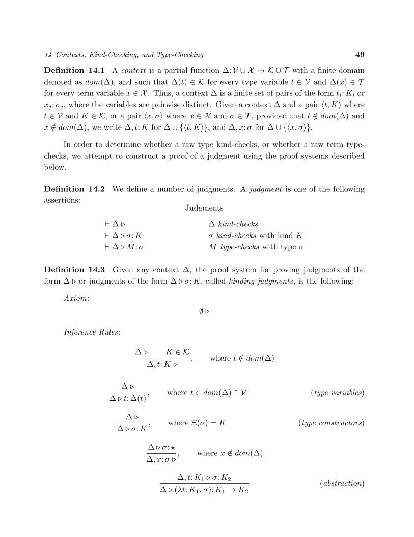
14 Contexts, Kind-Checking, and Type-Checking 49
Definition 14.1 A context is a partial function �:V [ X ! K [ T with a finite domain
denoted as dom(�), and such that �(t) 2 K for every type variable t 2 V and �(x) 2 Tfor every term variable x 2 X . Thus, a context � is a finite set of pairs of the form t
i
:Ki
or
xj
:�j
, where the variables are pairwise distinct. Given a context � and a pair ht,Ki wheret 2 V and K 2 K, or a pair hx,�i where x 2 X and � 2 T , provided that t /2 dom(�) and
x /2 dom(�), we write �, t:K for � [ {ht,Ki}, and �, x:� for � [ {hx,�i}.
In order to determine whether a raw type kind-checks, or whether a raw term type-
checks, we attempt to construct a proof of a judgment using the proof systems described
below.
Definition 14.2 We define a number of judgments. A judgment is one of the following
assertions:Judgments
` � . � kind-checks
` � . �:K � kind-checks with kind K
` � .M :� M type-checks with type �
Definition 14.3 Given any context �, the proof system for proving judgments of the
form � . or judgments of the form � . �:K, called kinding judgments, is the following:
Axiom:
; .
Inference Rules:
� . K 2 K�, t:K .
, where t /2 dom(�)
� .
� . t:�(t), where t 2 dom(�) \ V (type variables)
� .
� . �:K, where ⌅(�) = K (type constructors)
� . �: ?
�, x:� ., where x /2 dom(�)
�, t:K1 . �:K2
� . (�t:K1. �):K1 ! K2(abstraction)

50 ON GIRARD’S “CANDIDATS DE REDUCTIBILITE”
where t /2 FV(�(x)) for every x 2 dom(�) \ X
� . �:K1 ! K2 � . ⌧ :K1
� . �⌧ :K2(application)
� . �: ? � . ⌧ : ?
� . � ) ⌧ : ?())
� . �:K ! ?
� .⇧K
�: ?(⇧)
A context � kind-checks i↵ � . is provable. When a judgment � . �:K is provable,
we say that the type � kind-checks with kind K. It is not di�cult to show that if � . �:K
is provable, then � kind-checks. From now on, we assume that ⇥:⌃ ! T satisfies the
following property: if ⇥(f) = �, then . �: ? (recall that � has no free variables).
We extend ⌘↵
to (kinding) judgments as follows.
Definition 14.4 First, we define ↵-equivalence of contexts. Given two contexts � =
� [ {x1:�1, . . . , xn
:�n
} and �0 = � [ {x1:�01, . . . , xn
:�0n
}, where all pairs in � are of the
form t:K, t 2 V , K 2 K, we write � ⌘↵
�0 i↵ �i
⌘↵
�0i
for all i, 1 i n. Two kinding
judgments � . �:K and �0 . �0:K are ↵-equivalent i↵ � ⌘↵
�0 and � ⌘↵
�0.
In order to be able to manipulate ⌘↵
-equivalence classes of types, we add the following
inference rules to the proof system of definition 14.3.
� . �:K � ⌘↵
�0
�0 . �:K(⌘0
↵
)
� . �:K � ⌘↵
�0
� . �0:K(⌘00
↵
)
It it is not di�cult to show that if two kinding judgments � . �:K and �0 . �0:K
are ⌘↵
-equivalent and there is a proof ` � . �:K, then there is a proof ` �0 . �0:K.
Consequently, it is legitimate to identify ⌘↵
-equivalent types and contexts, and we will do
so from now on.
The types that kind-check form a simply-typed lambda calculus with set BK of base
types. Any two types that are �⌘-convertible will be considered equivalent. Thus, we review
the conversion rules for this calculus.
It is convenient to define reduction on raw types, and verify that it is kind-preserving
when applied to a type that kind-checks.
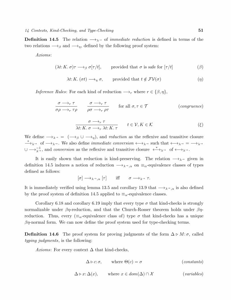
14 Contexts, Kind-Checking, and Type-Checking 51
Definition 14.5 The relation �!�
! of immediate reduction is defined in terms of the
two relations �!�
and �!⌘
, defined by the following proof system:
Axioms:
(�t:K. �)⌧ �!�
�[⌧/t], provided that � is safe for [⌧/t] (�)
�t:K. (�t) �!⌘
�, provided that t /2 FV(�) (⌘)
Inference Rules: For each kind of reduction �!r
where r 2 {�, ⌘},
� �!r
⌧
�⇢ �!r
⌧⇢
� �!r
⌧
⇢� �!r
⇢⌧for all �, ⌧ 2 T (congruence)
� �!r
⌧
�t:K. � �!r
�t:K. ⌧t 2 V,K 2 K (⇠)
We define �!�
! = (�!�
[ �!⌘
), and reduction as the reflexive and transitive closure⇤�!
�
! of �!�
! . We also define immediate conversion !�
! such that !�
! = �!�
!
[ �!�1�
! , and conversion as the reflexive and transitive closure⇤ !
�
! of !�
! .
It is easily shown that reduction is kind-preserving. The relation �!�
! given in
definition 14.5 induces a notion of reduction �!�
!,↵
on ⌘↵
-equivalence classes of types
defined as follows:
[�] �!�
!,↵
[⌧ ] i↵ � �!�
! ⌧.
It is immediately verified using lemma 13.5 and corollary 13.9 that �!�
!,↵
is also defined
by the proof system of definition 14.5 applied to ⌘↵
-equivalence classes.
Corollary 6.18 and corollary 6.19 imply that every type � that kind-checks is strongly
normalizable under �⌘-reduction, and that the Church-Rosser theorem holds under �⌘-
reduction. Thus, every (⌘↵
-equivalence class of) type � that kind-checks has a unique
�⌘-normal form. We can now define the proof system used for type-checking terms.
Definition 14.6 The proof system for proving judgments of the form � . M :�, called
typing judgments, is the following:
Axioms: For every context � that kind-checks,
� . c:�, where ⇥(c) = � (constants)
� . x:�(x), where x 2 dom(�) \ X (variables)

52 ON GIRARD’S “CANDIDATS DE REDUCTIBILITE”
Inference Rules:� .M :� ) ⌧ � .N :�
� .MN : ⌧(application)
�, x:� .M : ⌧
� . (�x:�. M):� ) ⌧(abstraction)
� .M :⇧K
� � . ⌧ :K
� .M⌧ :�⌧(type application)
�, t:K .M :�t
� . (⇤t:K.M):⇧K
�(type abstraction)
where in this rule, t /2 FV(�), and t /2 FV(�(x)) for every x 2 dom(�) \ X .
� . ⌧ : ? � .M :� �⇤ !
�
! ⌧
� .M : ⌧(type conversion)
If � .M :� is provable using the above proof system, we say that M type-checks with
type � under � and we write ` � .M :�. We say that the raw term M type-checks (or is
typable) i↵ there is some � and some � such that � .M :� is derivable. It is not di�cult
to show that if a typing judgment � .M :� is provable, then � kind-checks and � . �: ? is
provable.
In order to deal with ⌘↵
-equivalence, we define ⌘↵
-equivalent typing judgments as
follows.
Definition 14.7 Two typing judgments � . M :� and �0 . M 0:�0 are ↵-equivalent i↵
� ⌘↵
�0, M ⌘↵
M 0, and � ⌘↵
�0.
We also add the following inference rules to the proof system of definition 14.6.
� .M :� � ⌘↵
�0
�0 .M :�(⌘0
↵
)
� .M :� M ⌘↵
M 0
� .M 0:�(⌘00
↵
)
� .M :� � ⌘↵
�0
� .M :�0 (⌘000↵
)
Clearly, if � . M :� is provable, then � . �: ? and � . are also provable. It is not
di�cult to show that if two typing judgments � . M :� and �0 . M 0:�0 are ↵-equivalent
and there is a proof ` � .M :�, then there is a proof ` �0 .M 0:�0. Thus, it is legitimate to
work with equivalence classes of types, terms, and contexts, modulo ⌘↵
-equivalence. This
is also true for substitutions.

14 Contexts, Kind-Checking, and Type-Checking 53
Example 14.8 The following is a proof that M = ⇤t: ?. �x: t. x type-checks with type
8u: ?. (u) u) = ⇧?
(�u: ?. (u) u)).
t: ?, x: t . x: t
t: ? . (�x: t. x): (t) t) (t) t)⇤ !
�
! (�u: ?. (u) u))t
t: ? . (�x: t. x): (�u: ?. (u) u))t
. (⇤t: ?. �x: t. x):⇧?
(�u: ?. (u) u)).
Remark . It is also possible to formulate the typing rules for F!
by choosing 8 as a
primitive instead of ⇧. For instance, this is the choice adopted in Girard [10]. In this case,
we have the following two rules that replace type application and type abstraction:
� .M : 8t:K. � � . ⌧ :K
� .M⌧ :�[⌧/t](type application’)
�, t:K .M :�
� . (⇤t:K.M): 8t:K. �(type abstraction’)
where in this rule, t /2 FV(�(x)) for every x 2 dom(�) \ X .
Let F 0!
be this new system. Recall that if ⇧ is chosen as a primitive, then 8t:K. �
is an abbreviation for ⇧K
(�t:K. �). Then, using the fact that (�t:K. �)t �!�
! �, that
(�t:K. �)⌧ �!�
! �[⌧/t], and the type conversion rule, it is immediately verified by induc-
tion on the depth of proofs that every judgment � .M :� provable in F 0!
is also provable
in F!
(translating 8t:K. � in F 0!
to ⇧K
(�t:K. �) in F!
). Conversely, using the fact that
for every t /2 FV(�), 8t:K. (�t) = ⇧K
(�t:K. (�t)) �!⌘
⇧K
�, �⌧ = (�t)[⌧/t], and the type
conversion rule, it is immediately verified by induction on the depth of proofs that every
judgment � . M :� provable in F!
is also provable in F 0!
. Thus, the two proof systems
are equivalent. In the absence of ⌘-conversion (on types), it is an interesting exercise to
show that every proof in F!
can be converted into a proof in F 0!
(it can be shown that
⇧K
(�t:K. (�t)) and ⇧K
� are equivalent in F 0!
). Thus, F!
and F 0!
are also equivalent in
the absence of ⌘-conversion.
We can define the concept of the order of a kind or of a type. This will enable us to
define subsets of F!
.
Definition 14.9 The order of a kind K 2 K is defined inductively as follows:
ord(K) = 0, K 2 BK � {?}ord(?) = 1
ord(K1 ! K2) = max(ord(K1) + 1, ord(K2)).
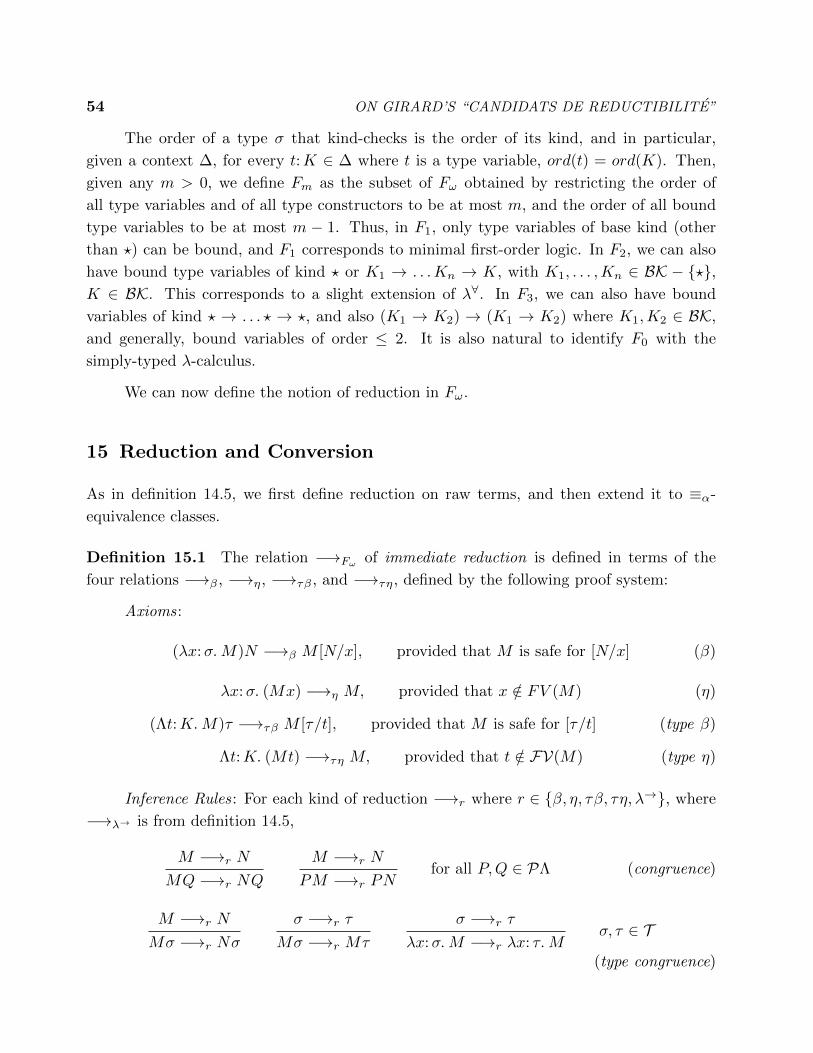
54 ON GIRARD’S “CANDIDATS DE REDUCTIBILITE”
The order of a type � that kind-checks is the order of its kind, and in particular,
given a context �, for every t:K 2 � where t is a type variable, ord(t) = ord(K). Then,
given any m > 0, we define Fm
as the subset of F!
obtained by restricting the order of
all type variables and of all type constructors to be at most m, and the order of all bound
type variables to be at most m � 1. Thus, in F1, only type variables of base kind (other
than ?) can be bound, and F1 corresponds to minimal first-order logic. In F2, we can also
have bound type variables of kind ? or K1 ! . . .Kn
! K, with K1, . . . ,Kn
2 BK � {?},K 2 BK. This corresponds to a slight extension of �8. In F3, we can also have bound
variables of kind ? ! . . . ? ! ?, and also (K1 ! K2) ! (K1 ! K2) where K1,K2 2 BK,
and generally, bound variables of order 2. It is also natural to identify F0 with the
simply-typed �-calculus.
We can now define the notion of reduction in F!
.
15 Reduction and Conversion
As in definition 14.5, we first define reduction on raw terms, and then extend it to ⌘↵
-
equivalence classes.
Definition 15.1 The relation �!F! of immediate reduction is defined in terms of the
four relations �!�
, �!⌘
, �!⌧�
, and �!⌧⌘
, defined by the following proof system:
Axioms:
(�x:�. M)N �!�
M [N/x], provided that M is safe for [N/x] (�)
�x:�. (Mx) �!⌘
M, provided that x /2 FV (M) (⌘)
(⇤t:K.M)⌧ �!⌧�
M [⌧/t], provided that M is safe for [⌧/t] (type �)
⇤t:K. (Mt) �!⌧⌘
M, provided that t /2 FV(M) (type ⌘)
Inference Rules : For each kind of reduction �!r
where r 2 {�, ⌘, ⌧�, ⌧⌘,�!}, where�!
�
! is from definition 14.5,
M �!r
N
MQ �!r
NQ
M �!r
N
PM �!r
PNfor all P,Q 2 P⇤ (congruence)
M �!r
N
M� �!r
N�
� �!r
⌧
M� �!r
M⌧
� �!r
⌧
�x:�. M �!r
�x: ⌧. M�, ⌧ 2 T
(type congruence)
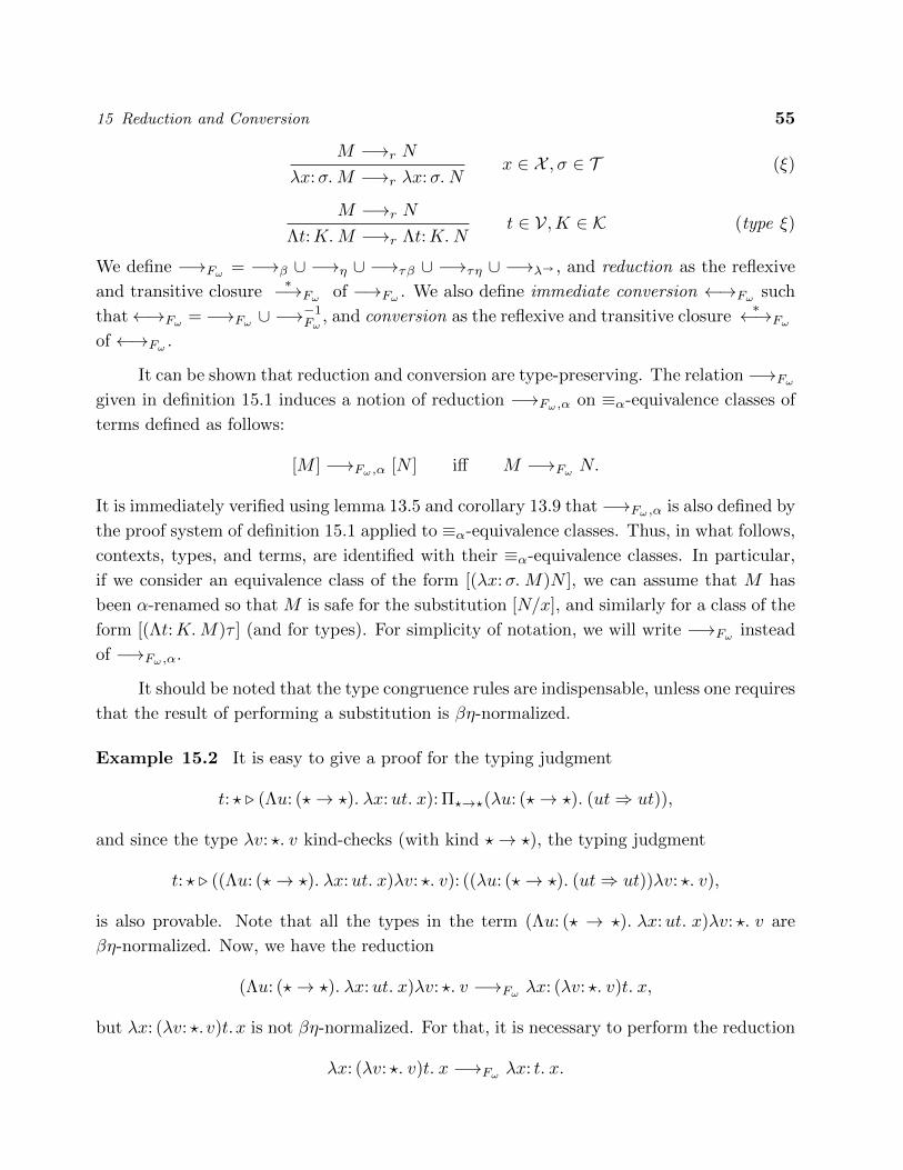
15 Reduction and Conversion 55
M �!r
N
�x:�. M �!r
�x:�. Nx 2 X ,� 2 T (⇠)
M �!r
N
⇤t:K.M �!r
⇤t:K. Nt 2 V,K 2 K (type ⇠)
We define �!F! = �!
�
[ �!⌘
[ �!⌧�
[ �!⌧⌘
[ �!�
! , and reduction as the reflexive
and transitive closure⇤�!
F! of �!F! . We also define immediate conversion !
F! such
that !F! = �!
F! [ �!�1F!
, and conversion as the reflexive and transitive closure⇤ !
F!
of !F! .
It can be shown that reduction and conversion are type-preserving. The relation �!F!
given in definition 15.1 induces a notion of reduction �!F!,↵
on ⌘↵
-equivalence classes of
terms defined as follows:
[M ] �!F!,↵
[N ] i↵ M �!F! N.
It is immediately verified using lemma 13.5 and corollary 13.9 that �!F!,↵
is also defined by
the proof system of definition 15.1 applied to ⌘↵
-equivalence classes. Thus, in what follows,
contexts, types, and terms, are identified with their ⌘↵
-equivalence classes. In particular,
if we consider an equivalence class of the form [(�x:�. M)N ], we can assume that M has
been ↵-renamed so that M is safe for the substitution [N/x], and similarly for a class of the
form [(⇤t:K.M)⌧ ] (and for types). For simplicity of notation, we will write �!F! instead
of �!F!,↵
.
It should be noted that the type congruence rules are indispensable, unless one requires
that the result of performing a substitution is �⌘-normalized.
Example 15.2 It is easy to give a proof for the typing judgment
t: ? . (⇤u: (?! ?). �x:ut. x):⇧?!?
(�u: (?! ?). (ut) ut)),
and since the type �v: ?. v kind-checks (with kind ?! ?), the typing judgment
t: ? . ((⇤u: (?! ?). �x:ut. x)�v: ?. v): ((�u: (?! ?). (ut) ut))�v: ?. v),
is also provable. Note that all the types in the term (⇤u: (? ! ?). �x:ut. x)�v: ?. v are
�⌘-normalized. Now, we have the reduction
(⇤u: (?! ?). �x:ut. x)�v: ?. v �!F! �x: (�v: ?. v)t. x,
but �x: (�v: ?. v)t.x is not �⌘-normalized. For that, it is necessary to perform the reduction
�x: (�v: ?. v)t. x �!F! �x: t. x.
56 ON GIRARD’S “CANDIDATS DE REDUCTIBILITE”
We also have the reduction sequence
(�u: (?! ?). (ut) ut))�v: ?. v �!F! ((�v: ?. v)t) (�v: ?. v)t)
⇤�!F! (t) t).
Note that the typing judgment t: ? . (�x: t. x): (t) t) is provable.
16 The Method of Candidates
We now generalize the method of candidates to F!
. The proof that we sketch is modelled
after Girard’s original proof, and only di↵ers in the notation and in the fact that we present
it in a slightly more general setting, using T -closed families, and closed families of Girard
sets. As pointed out by Thierry Coquand, it is possible to prove strong normalization for F!
using an untyped version of the candidates and the erasing trick. However, the typed version
seems necessary when the system F!
is enriched, for example with first-order rewriting, and
we present the typed version. The main complication is that we now have new types formed
by �-abstraction and application. Thus, it is necessary to define candidates of reducibility
by induction on the kind of types. As before, let C�
denote the set of candidates of type �.
For types of kind ?, basically nothing changes. For a type � of kind K1 ! K2, a candidate
of type � is any function
f :[
⌧ :K1
{⌧}⇥ C⌧
![
⌧ :K1
C�⌧
such that f(⌧, C) 2 C�⌧
for every C 2 C⌧
and satisfying a technical condition listed in
definition 16.2.
Actually, there is a problem with this definition, namely that types may contain type
variables, and in order for these types to kind-check, we need to assume that the type
variables have been assigned kinds. There are two ways to overcome this problem. The first
solution, which is the solution adopted by Coquand in his proof of normalization for the
theory of constructions [5], is to define the notion of a candidate of type � . �:K, where
� . �:K kind-checks. In this approach, we deal with families C�.�:K of sets of candidates
indexed by provable kinding judgments. Roughly, a candidate C of type � . �:K is a set
of provable typing judgments of the form �0 .M :� where � ✓ �0, and satisfying certain
properties as in definition 7.8. If this approach is followed, it is also necessary to define
[[� . �:K]]✓⌘, as opposed to simply [[�]]✓⌘. The proof can be carried out, but the notation
is quite formidable.
However, in F!
, since the fact that a type kind-checks only depends on assigning kinds
to types variables, and kinds are independent of the types, there is a second simpler solution
16 The Method of Candidates 57
(adopted by Girard). This second solution is to relativize the definition of a family of sets
of candidates to a global kind assignment :V ! K. This way, we can deal with types �
that kind-check under some context that agrees with on V. We also assume that is
extended to the type constructors, so that it agrees with ⌅ on T C. The above discussion
leads to the following definition.
Definition 16.1 Given a kind assignment :V ! K, we let T |
be the set of all types
� that “kind-check under ”, that is, such that � . �:K is provable for some kind K 2 Kand some context � whose restriction to V agrees with . Given :V ! K, for every type
� 2 T |
of kind ?, we let PT�
be the set of all provable typing judgments of the form
� .M :�, where � is any context whose restriction to V agrees with .
We will use the abbreviation � .M 2 S for � .M :� 2 S when S is a subset of PT�
.
We also use the notation �:K 2 T |
to express the fact that � kind-checks with kind K
under , and �, . M :� to mean that �0 . M :� is provable for some (finite) context �0
such that � ✓ �0 and the restriction of �0 to V agrees with .
Given any two types �, ⌧ 2 T |
of kind ? and any two sets S ✓ PT�
and T ✓ PT⌧
,
we let [S ) T ] be the subset of PT�)⌧
defined as before:
[S ) T ] = {� .M 2 PT�)⌧
| 8�0 .N, if � ✓ �0 and �0 .N 2 S, then �0 .MN 2 T}.
Given a kind assignment :V ! K, a T |
-closed family is defined as follows.
Definition 16.2 Let C = (C�
)�2T | be a T |
-indexed family where for each �, if � is of
kind ? then C�
is a nonempty set of subsets of PT�
, else if � is of kind K1 ! K2 then C�
is
a nonempty set of functions fromS
⌧ :K1{⌧}⇥ C
⌧
toS
⌧ :K1C�⌧
, and the following properties
hold:
(1) For every � 2 T |
of kind ?, every C 2 C�
is a nonempty subset of PT�
.
(2) For every �, ⌧ 2 T |
of kind ?, for every C 2 C�
and D 2 C⌧
, we have [C ) D] 2 C�)⌧
.
(3) For every � 2 T |
of kind K ! ?, for every ⌧ 2 T |
of kind K, for every family
(A⌧,C
)⌧2T |,C2C⌧
, where each set A⌧,C
is in C�⌧
, we have
{� .M 2 PT ⇧K�
| 8(⌧ :K) 2 T |
, �, .M⌧ 2\
C2C⌧
A⌧,C
} 2 C⇧K�
.
(4) For every � 2 T |
of kind K1 ! K2,
C�
= {f :[
⌧ :K12T |
{⌧}⇥ C⌧
58 ON GIRARD’S “CANDIDATS DE REDUCTIBILITE”
A family satisfying the above conditions is called a T |
-closed family .
Definition 16.3 Let C be a T |
-closed family. A pair h✓, ⌘i where ✓:V ! T |
is a
substitution and ⌘: T C [ V !S
C is a candidate assignment i↵ for every t 2 V , (t) = K
implies that ✓(t):K 2 T |
, ⌘(t) 2 C✓(t), and ⌘(�) 2 C
�
for every � 2 T C.
We can associate certain sets of provable typing judgments to the types inductively
as explained below.
Definition 16.4 Given any candidate assignment h✓, ⌘i, for every type � 2 T |
, we define
[[�]]✓⌘ as follows:
[[t]]✓⌘ = ⌘(t), whenever t 2 T C [ V;[[(� ) ⌧)]]✓⌘ = [[[�]]✓⌘ ) [[⌧ ]]✓⌘];
[[⇧K
�]]✓⌘ = {� .M 2 PT✓(⇧K�) | 8(⌧ :K) 2 T |
,
�, .M⌧ 2\
C2C⌧
[[�]]✓⌘(⌧, C)};
[[�⌧ ]]✓⌘ = [[�]]✓⌘(✓(⌧), [[⌧ ]]✓⌘);
[[�t:K. �]]✓⌘ = �⌧�C 2 C⌧ :K . [[�]]✓[t := ⌧ ]⌘[t := C].
In the last clause of this definition, �⌧�C 2 C⌧ :K . [[�]]✓[t := ⌧ ]⌘[t := C] denotes the function
f such that f(⌧, C) = [[�]]✓[t := ⌧ ]⌘[t := C] for every C 2 C⌧
such that ⌧ 2 T |
is of kind
K.
The following technical lemmas will be useful later.
Lemma 16.5 Given any candidate assignments h✓1, ⌘1i and h✓2, ⌘2i, for every � 2 T |
, if
✓1, ✓2 agree on FV(�), and ⌘1, ⌘2 agree on FV(�) and T C, then [[�]]✓1⌘1 = [[�]]✓2⌘2.
Proof . Easy induction on the structure of types.
Lemma 16.6 Given any two types �, ⌧ 2 T |
, for every candidate assignment h✓, ⌘i,
[[�[⌧/t]]]✓⌘ = [[�]]✓[t := ✓(⌧)]⌘[t := [[⌧ ]]✓⌘].
Proof . Straightforward induction on the structure of �.
The following lemma is crucial and shows that [[�]]✓⌘ actually has a constant value on
the equivalence class of � modulo �!-convertibility.
16 The Method of Candidates 59
Lemma 16.7 For every candidate assignment h✓, ⌘i, for every two types �,�0 2 T |
, if
�⇤ !
�
! �0, then [[�]]✓⌘ = [[�0]]✓⌘.
Proof . It is su�cient to prove that if �⇤�!
�
! �0, then [[�]]✓⌘ = [[�0]]✓⌘. The proof proceeds
by induction on the proof that �⇤�!
�
! �0. The only nontrivial cases are � and ⌘-conversion,
and those are handled using lemma 16.6 and lemma 16.5.
We now have a version of “Girard’s trick” for F!
.
Lemma 16.8 (Girard) If C is a T |
-closed family, for every candidate assignment h✓, ⌘i,for every type �, then [[�]]✓⌘ 2 C
✓(�).
Proof . The lemma is proved by induction on the structure of types. The only case worth
mentioning is the case of a typed �-abstraction. By ↵-renaming, it can be assumed that
�t:K.� is safe for ✓. In this case, we use lemma 16.7 and the fact that (�t:K.✓(�))⌧ �!�
!
✓(�)[⌧/t], and that because �t:K. � is safe for ✓, ✓(�)[⌧/t] = ✓[t := ⌧ ](�).
In order to use lemma 16.8 in proving properties of polymorphic lambda calculi, we
need to define T |
-closed families satisfying some additional properties.
Definition 16.9 We say that a T |
-indexed family C is a family of sets of candidates of
reducibility i↵ it is T |
-closed and satisfies the conditions listed below.22
R0. Whenever � .M 2 C and � ✓ �0, then �0 .M 2 C.
R1. For every �: ? 2 T |
, for every set C 2 C�
, � . x 2 C, for every x:� 2 �,
For every �: ? 2 T |
where � = ⇥(f), for every set C 2 C�
, � . f 2 C, for every
f 2 ⌃.
R2. (i) For all �: ?, ⌧ : ? 2 T |
, for every C 2 C⌧
, for all �,�0, if
� .M 2[
C⌧
,
�0 .N 2[
C�
, and
�0 .M [N/x] 2 C, then
�0 . (�x:�. M)N 2 C.
(ii) For every � 2 T |
of kind K ! ?, every ⌧ 2 T |
of kind K, for every C 2 C�⌧
,
for all �,�0, if
� .M 2[
C�t
and
�0 .M [⌧/t] 2 C, then
�0 . (⇤t:K.M)⌧ 2 C.
Lemma 7.9 generalizes to F!
as follows.
22 Again, we also have to assume that every C 2 C is closed under ↵-equivalence.

60 ON GIRARD’S “CANDIDATS DE REDUCTIBILITE”
Lemma 16.10 (Girard) Let C = (C�
)�2T | be a family of sets of candidates of reducibility.
For every � . M 2 PT�
, for every candidate assignment h✓, ⌘i, for every substitution
':�! �, if ✓(�), . '(x) 2 [[�(x)]]✓⌘ for x 2 FV (M), then ✓(�), . '(✓(M)) 2 [[�]]✓⌘.
Proof . It is similar to the proof of lemma 7.9 and proceeds by induction on the depth of
the proof tree for � .M :�. Type conversion is handled using lemma 16.7. We only sketch
the verification for two of the other cases.
Case 1.�, t:K .M :�t
� . (⇤t:K.M):⇧K
�(type abstraction)
where in this rule, t /2 FV(�), and t /2 FV(�(x)) for every x 2 dom(�) \ X .
Given any ⌧ 2 T |
, the induction hypothesis applies to �, t:K . M :�t and to any
candidate assignment h✓[t := ⌧ ], ⌘[t := C]i where C 2 C⌧
and ⌧ :K 2 T |
(and by suitable ↵-
renaming, t /2 FV(�(x)) for every x 2 dom(�), and the safeness conditions for substitution
hold). Thus, ✓[t := ⌧ ](�) = ✓(�), and due to the proviso on the inference rule, ✓[t :=
⌧ ](�) = ✓(�), and ✓[t := ⌧ ](M) = ✓(M)[⌧/t]. Thus, we have
✓(�), . '(✓(M))[⌧/t] 2 [[�t]]✓[t := ⌧ ]⌘[t := C].
In particular, this holds for ⌧ = t, and so ✓(�), . '(✓(M)) 2SC✓(�t). Then, by (R2)(ii),
✓(�), . (⇤t:K. '(✓(M)))⌧ 2 [[�t]]✓[t := ⌧ ]⌘[t := C],
that is, ✓(�), . '(✓(⇤t:K.M))⌧ 2 [[�t]]✓[t := ⌧ ]⌘[t := C].
Again, due to the the proviso on the rule, [[�]]✓[t := ⌧ ]⌘[t := C] = [[�]]✓⌘, and since
[[�t]]✓[t := ⌧ ]⌘[t := C] = [[�]]✓[t := ⌧ ]⌘[t := C](✓[t := ⌧ ](t), [[t]]✓[t := ⌧ ]⌘[t := C])
and [[t]]✓[t := ⌧ ]⌘[t := C] = C, ✓[t := ⌧ ](t) = ⌧ , we have
[[�t]]✓[t := ⌧ ]⌘[t := C] = [[�]]✓⌘(⌧, C).
Thus, ✓(�), . '(✓(⇤t:K. M))⌧ 2 [[�]]✓⌘(⌧, C) for all C 2 C⌧
such that ⌧ :K 2 T |
, which
proves that
✓(�) . '(✓(⇤t:K.M)) 2 [[⇧K
�]]✓⌘.
Case 2.� .M :⇧
K
� � . ⌧ :K
� .M⌧ :�⌧(type application)

16 The Method of Candidates 61
By the induction hypothesis, ✓(�), . '(✓(M)) 2 [[⇧K
�]]✓⌘, and so
✓(�), . '(✓(M))� 2 [[�]]✓⌘(�, C)
for every C 2 C�
where �:K 2 T |
. By choosing � = ✓(⌧), C = [[⌧ ]]✓⌘, and using the fact
that '(✓(M))✓(⌧) = '(✓(M⌧)) and [[�⌧ ]]✓⌘ = [[�]]✓⌘(✓(⌧), [[⌧ ]]✓⌘), we have
✓(�), . '(✓(M⌧)) 2 [[�⌧ ]]✓⌘,
as desired.
As for �8, in order to show the existence of families of candidates of reducibility, we
need stronger conditions. One can define saturated sets as in section 8, or Girard sets as in
section 9. We shall present the version of the Girard sets, leaving the other version as an
exercise to the reader.
A simple term is defined as in definition 9.1, that is, a term M is simple i↵ it is either
a variable x, a constant f 2 ⌃, an application MN , or a type application M⌧ .
Definition 16.11 Let S = (S�
)�:?2T | be a family such that each S
�
is a nonempty
subset of PT�
.23 For every type �: ? 2 T |
, a subset C of S�
is a Girard set of type � i↵
the following conditions hold:24
CR0. Whenever � .M 2 C and � ✓ �0, then �0 .M 2 C.
CR1. If � .M 2 C, then M is SN w.r.t. �!F! ;
CR2. If � .M 2 C and M �!F! N , then � .N 2 C;
CR3. For every simple term �.M 2 PT�
, if �.N 2 C for every N such that M �!F! N ,
then � .M 2 C.
Note that (CR3) implies that all simple irreducible terms are in C. Also, (CR1),
(CR2), and (CR3) are defined w.r.t. �!F! , which means that �⌘-reduction on types is
taken into account. This is crucial for proving strong normalization.
Definition 16.12 Let S = (S�
)�:?2T | be a family such that each S
�
is a nonempty
subset of PT�
. We say that S is closed i↵ for all �: ?, ⌧ : ? 2 T |
, for every x 2 X , if
� .M 2 PT�)⌧
and �, x:� .Mx 2 S⌧
, then � .M 2 S�)⌧
, and for every t:K 2 T |
and
�:K 2 T |
, if � .M 2 PT ⇧K�
and �, t:K .Mt 2 S�t
then � .M 2 S⇧K�
.
We have the following generalization of lemma 9.4.
23 Note that S = (S�)�:?2T | is not a T |-indexed family. It is indexed by the set of types of kind ?.24 We also have to assume that every Girard subset of S is closed under ↵-equivalence.

62 ON GIRARD’S “CANDIDATS DE REDUCTIBILITE”
Lemma 16.13 (Girard) Let S = (S�
)�:?2T | be a closed family where each S
�
is a
nonempty subset of PT�
, and let C be the T |
-indexed family such that for each �: ? 2 T |
,
C�
is the set of Girard subsets of S�
, and for �:K1 ! K2 2 T |
, C�
is defined as in clause
(4) of definition 16.2. If S�
2 C�
for every �: ? 2 T |
(i.e. S�
is a Girard subset of itself),
then C is a family of sets of candidates of reducibility.
Proof . It is similar to the proof of lemmas 9.3 and 9.4. A subtlety arises in proving that
(R2) holds. We proceed as in the proof that (S2) holds (given in lemma 9.3), that is, we
show that � . Q 2 C whenever (�x:�. M)N �!F! Q, and that � . Q 2 C whenever
(⇤t:K.M)⌧ �!F! Q, assuming that M and N are SN. However, � or ⌧ can be �⌘-reduced,
and we also need to prove that �⌘-reduction on types (�!�
!) is strongly normalizing.
Fortunately, this is a special case of corollary 6.18, as observed earlier.
It is also necessary to verify conditions (1), (2), (3), (4) of definition 16.2. This is
done by induction on kinds, and for the kind ? by induction on types. Verifying (1), (2),
(3) is done as in lemma 9.4. We still need to check (4), that for a type �:K1 ! K2 2 T |
,
C�
is nonempty. This is done by induction on K1 ! K2. The base case holds since
can�
= S�
2 C�
for every �: ? 2 T |
. For �:K1 ! K2 2 T |
, for every ⌧ :K1 2 T |
, since
�⌧ :K2 2 T |
, by the induction hypothesis there is some function can�⌧
2 C�⌧
, and so the
function can�
such that can�
(⌧, C) = can�⌧
for every C 2 C⌧
(⌧ :K1 2 T |
) is in C�
.
We now have a version of Girard’s fundamental theorem for F!
.
Theorem 16.14 (Girard) Let S = (S�
)�:?2T | be a closed family where each S
�
is a
nonempty subset of PT�
, let C be the T |
-indexed family of sets defined in lemma 16.13,
and assume that S�
2 C�
for every �: ? 2 T |
. For every �.M 2 PT�
, we have �.M 2 S�
.
Proof . By lemma 16.13, C is a family of sets of candidates of reducibility. We now apply
lemma 16.10 to any assignment (for example, the assignment with value ⌘(t) = cant
), the
identity type substitution, and the identity term substitution, which is legitimate since by
(CR3), every variable belongs to every Girard set.25
Remark : Thierry Coquand pointed out to us that because �⌘-reduction on types
(�!�
!) is strongly normalizing, an untyped version of the candidates using the erasing
trick works for F!
. The function Erase:P⇤! ⇤ for F!
is defined recursively as follows:
Erase(c) = c, whenever c 2 ⌃,
Erase(x) = x, whenever x 2 X ,
Erase(MN) = Erase(M)Erase(N),
Erase(�x:�. M) = �x. Erase(M),
25 Actually, some ↵-renaming may have to be performed on M and � so that they are both safe for thetype and term identity substitution.

16 The Method of Candidates 63
Erase(M�) = Erase(M),
Erase(�t:K.M) = Erase(M).
However, obtaining the confluence property using the erasing trick is an open problem.
The next lemma is a generalization of lemma 10.2 and gives interesting examples of closed
families of Girard sets.
Lemma 16.15 (i) The family SN�
such that for every �: ? 2 T |
, SN�,�
is the set
of typing judgments � . M :� provable in F!
such that M is strongly normalizing under
�-reduction, is a closed family of Girard sets. (ii) The family SN�⌘
such that for every
�: ? 2 T |
, SN�⌘,�
is the set of typing judgments � .M :� provable in F!
such that M is
strongly normalizing under �⌘-reduction, is a closed family of Girard sets. (iii) The family
consisting for every �: ? 2 T |
of the set of typing judgments � .M :� provable in F!
such
that confluence under �-reduction holds from M and all of its subterms, is a closed family
of Girard sets. (iv) The family consisting for every �: ? 2 T |
of the set of typing judgments
� .M :� provable in F!
such that confluence under �⌘-reduction holds from M and all of
its subterms, is a closed family of Girard sets.
Proof . (i)-(ii) It is trivial to verify that closure and (CR0)–(CR3) hold. (iii)-(iv) The proof
is similar to the one given in appendix 2.
It should be noted that the fact that the above results are relativized to a type assign-
ment is really not a restriction. Indeed, we could assume that the set of type variables
is partitioned into a family of countable sets, one for each kind. Thus, we can assume that
we are dealing with a single .
The system F!
can be extended in several ways. For example, product types and
existential types can be added. In fact, such an extension is studied in Girard’s thesis [10],
including disjunctive types. Strong normalization still holds. Another way of extending
F!
is to allow a richer class of kinds and types. This can be achieved by allowing term
variables in types and the formation of new types by �-abstraction over these variables. At
the same time, richer kinds are allowed, namely dependent products. Such a system, the
theory of constructions, was invented by Coquand [5, 7]. The theory of constructions is
also investigated in Huet and Coquand [6]. A related system, LF, has been investigated by
Harper, Honsell, and Plotkin [13, 14]. Strong normalization holds for these systems. For
the theory of construction, the proof uses Girard’s method of candidates of reducibility and
follows the general scheme used in the proof of strong normalization for F!
, but it is more
complex because types may contain terms. The problem is that it is no longer possible to
prove first that �⌘-reduction is strongly normalizing on types. Roughly, one needs to define
[[� . �:K]]✓⌘ and [[� .K:Kind]]✓⌘. For details, the interested (and perseverant) reader is
referred to Coquand [5]. A proof of strong normalization for the theory of constructions is

64 ON GIRARD’S “CANDIDATS DE REDUCTIBILITE”
also given in Seldin [33], which also contains an extensive study of type systems including
�8 and the theory of constructions. For LF, a proof of strong normalization consists in
mapping LF into the simply-typed lambda calculus. For details, the reader should consult
[14]. Other interesting work on the theory of constructions and F!
appears in Paulin-
Morhing [26], where it is shown how programs and their proofs can be extracted. Related
work is done in Pfenning [28].
Acknowledgment. I am grateful to Jean Yves Girard for providing invaluable inspi-
ration, advice, and encouragement. I also wish to thank Val Breazu-Tannen, Pierre Louis
Curien, Bob Harper, Zhaohui Luo, and Kathleen Milsted, for looking at this paper very
carefully and for their help and advice with the correctness and the presentation. Val caught
some bugs and gave me advice for simplifying the notation, Bob and Kathleen read the en-
tire manuscript and contributed a large number of improvements. Zhaohui Luo pointed out
to me the necessity of condition (CR2), which I had overlooked in earlier versions. Pierre
Louis Curien and Roberto Di Cosmo reported a gap in the proof of lemma 9.3. Finally,
I wish to thank Thierry Coquand, Gerard Huet, Tomas Isakowitz, John Mitchell, Frank
Pfenning, Andre Scedrov, Wayne Snyder, and Rick Statman, for their comments.
17 Appendix 1: Product Types in F!
In this section, we extend the system F!
by allowing product types. An even more general
system with disjunctive and existential types was investigated by Girard [10].
In the formula–as–type analogy, product types correspond to conjunctions, and the
typing rules correspond to the introduction and elimination rules for conjunction. We will
be dealing with product types with surjective pairing.
The definition of the kinds given in definition 12.1 remains unchanged. However, it
is assumed that every set T C of type constructors contains the special symbols ⇥, ) and
⇧K
for every K 2 K. The type constructor ⇥ is the product type constructor. The type
constructors are assigned kinds by a kind signature.
Definition 17.1 A kind signature is a function ⌅: T C ! K assigning a kind to every
type constructor in T C, and such that ⌅()) = ? ! (? ! ?), ⌅(⇥) = ? ! (? ! ?), and
⌅(⇧K
) = (K ! ?)! ?.
The definition of raw types remains unchanged, but since ⇥ belongs to every set T Cof type constructors, more raw types are allowed. The definition is repeated for the reader’s
convenience.
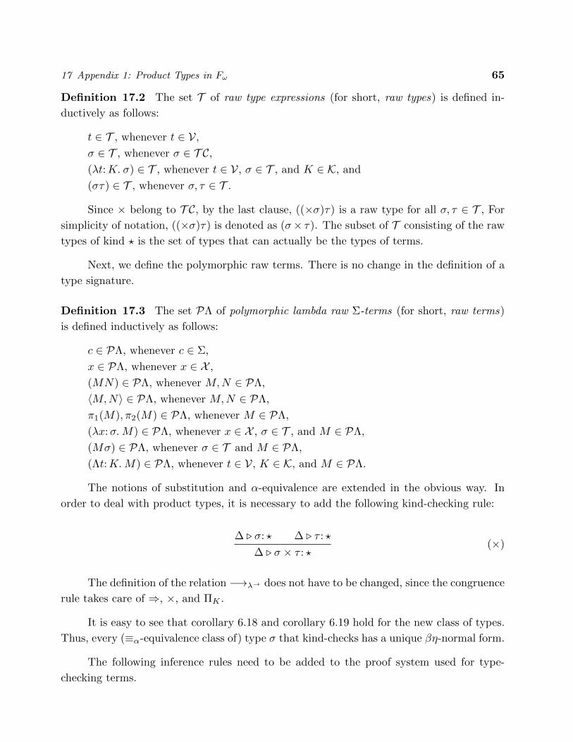
17 Appendix 1: Product Types in F! 65
Definition 17.2 The set T of raw type expressions (for short, raw types) is defined in-
ductively as follows:
t 2 T , whenever t 2 V,� 2 T , whenever � 2 T C,(�t:K. �) 2 T , whenever t 2 V, � 2 T , and K 2 K, and
(�⌧) 2 T , whenever �, ⌧ 2 T .
Since ⇥ belong to T C, by the last clause, ((⇥�)⌧) is a raw type for all �, ⌧ 2 T , For
simplicity of notation, ((⇥�)⌧) is denoted as (�⇥ ⌧). The subset of T consisting of the raw
types of kind ? is the set of types that can actually be the types of terms.
Next, we define the polymorphic raw terms. There is no change in the definition of a
type signature.
Definition 17.3 The set P⇤ of polymorphic lambda raw ⌃-terms (for short, raw terms)
is defined inductively as follows:
c 2 P⇤, whenever c 2 ⌃,
x 2 P⇤, whenever x 2 X ,
(MN) 2 P⇤, whenever M,N 2 P⇤,
hM,Ni 2 P⇤, whenever M,N 2 P⇤,
⇡1(M),⇡2(M) 2 P⇤, whenever M 2 P⇤,
(�x:�. M) 2 P⇤, whenever x 2 X , � 2 T , and M 2 P⇤,
(M�) 2 P⇤, whenever � 2 T and M 2 P⇤,
(⇤t:K.M) 2 P⇤, whenever t 2 V, K 2 K, and M 2 P⇤.
The notions of substitution and ↵-equivalence are extended in the obvious way. In
order to deal with product types, it is necessary to add the following kind-checking rule:
� . �: ? � . ⌧ : ?
� . � ⇥ ⌧ : ?(⇥)
The definition of the relation �!�
! does not have to be changed, since the congruence
rule takes care of ), ⇥, and ⇧K
.
It is easy to see that corollary 6.18 and corollary 6.19 hold for the new class of types.
Thus, every (⌘↵
-equivalence class of) type � that kind-checks has a unique �⌘-normal form.
The following inference rules need to be added to the proof system used for type-
checking terms.
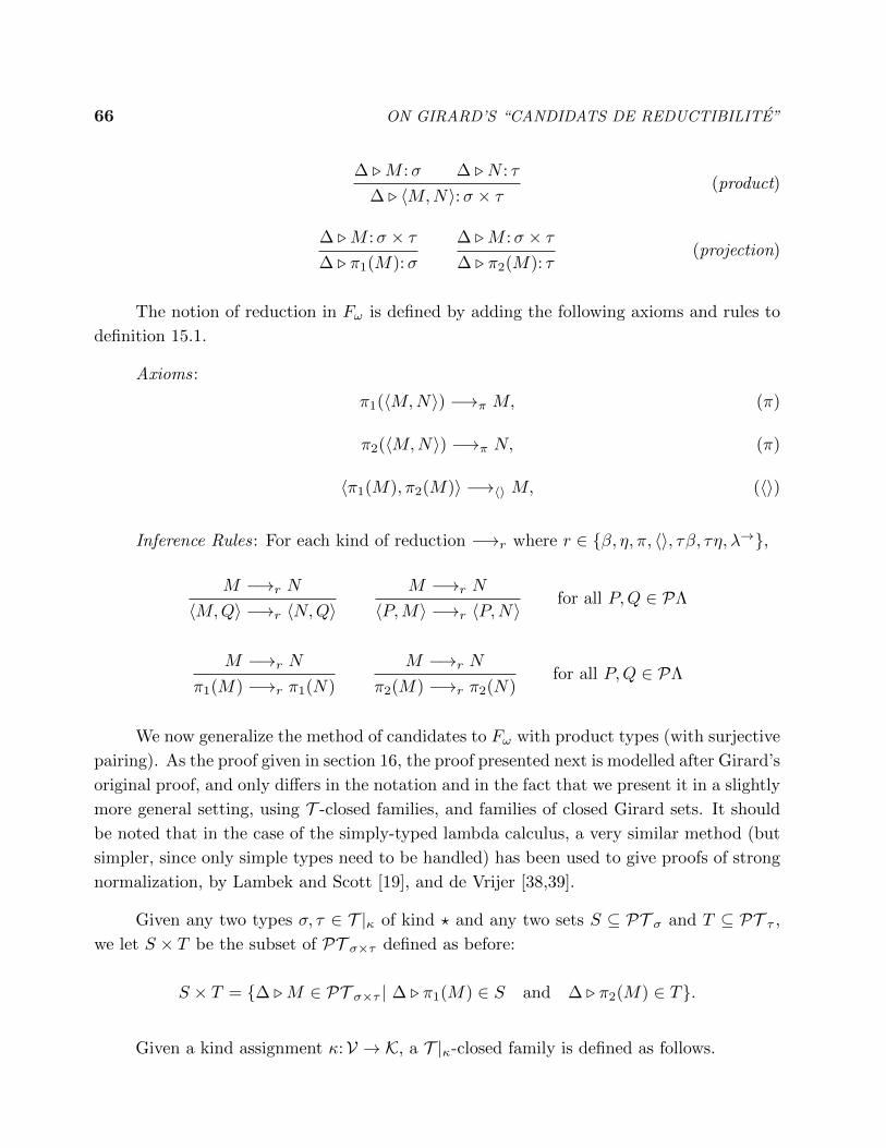
66 ON GIRARD’S “CANDIDATS DE REDUCTIBILITE”
� .M :� � .N : ⌧
� . hM,Ni:� ⇥ ⌧(product)
� .M :� ⇥ ⌧
� . ⇡1(M):�
� .M :� ⇥ ⌧
� . ⇡2(M): ⌧(projection)
The notion of reduction in F!
is defined by adding the following axioms and rules to
definition 15.1.
Axioms:
⇡1(hM,Ni) �!⇡
M, (⇡)
⇡2(hM,Ni) �!⇡
N, (⇡)
h⇡1(M),⇡2(M)i �!hi M, (hi)
Inference Rules: For each kind of reduction �!r
where r 2 {�, ⌘,⇡, hi, ⌧�, ⌧⌘,�!},
M �!r
N
hM,Qi �!r
hN,QiM �!
r
N
hP,Mi �!r
hP,Nifor all P,Q 2 P⇤
M �!r
N
⇡1(M) �!r
⇡1(N)
M �!r
N
⇡2(M) �!r
⇡2(N)for all P,Q 2 P⇤
We now generalize the method of candidates to F!
with product types (with surjective
pairing). As the proof given in section 16, the proof presented next is modelled after Girard’s
original proof, and only di↵ers in the notation and in the fact that we present it in a slightly
more general setting, using T -closed families, and families of closed Girard sets. It should
be noted that in the case of the simply-typed lambda calculus, a very similar method (but
simpler, since only simple types need to be handled) has been used to give proofs of strong
normalization, by Lambek and Scott [19], and de Vrijer [38,39].
Given any two types �, ⌧ 2 T |
of kind ? and any two sets S ✓ PT�
and T ✓ PT⌧
,
we let S ⇥ T be the subset of PT�⇥⌧
defined as before:
S ⇥ T = {� .M 2 PT�⇥⌧
| � . ⇡1(M) 2 S and � . ⇡2(M) 2 T}.
Given a kind assignment :V ! K, a T |
-closed family is defined as follows.

17 Appendix 1: Product Types in F! 67
Definition 17.4 Let C = (C�
)�2T | be a T |
-indexed family where for each �, if � is of
kind ? then C�
is a nonempty set of subsets of PT�
, else if � is of kind K1 ! K2 then C�
is
a nonempty set of functions fromS
⌧ :K1{⌧}⇥ C
⌧
toS
⌧ :K1C�⌧
, and the following properties
hold:
(1) For every � 2 T |
of kind ?, every C 2 C�
is a nonempty subset of PT�
.
(2) For every �, ⌧ 2 T |
of kind ?, for every C 2 C�
and D 2 C⌧
, we have [C ) D] 2 C�)⌧
.
(3) For every � 2 T |
of kind K ! ?, for every ⌧ 2 T |
of kind K, for every family
(A⌧,C
)⌧2T |,C2C⌧
, where each set A⌧,C
is in C�⌧
, we have
{� .M 2 PT ⇧K�
| 8(⌧ :K) 2 T |
, �, .M⌧ 2\
C2C⌧
A⌧,C
} 2 C⇧K�
.
(4) For every � 2 T |
of kind K1 ! K2,
C�
= {f :[
⌧ :K12T |
{⌧}⇥ C⌧
![
⌧ :K12T |
C�⌧
such that f(⌧, C) 2 C�⌧
for every C 2 C⌧
, and
f(⌧1, C) = f(⌧2, C) whenever ⌧1⇤ !
�
! ⌧2}.
(5) For every �, ⌧ 2 T |
of kind ?, for every C 2 C�
and D 2 C⌧
, we have C ⇥D 2 C�⇥⌧
.
A family satisfying the above conditions is called a T |
-closed family .
We associate certain sets of provable typing judgments to the types inductively as
explained below.
Definition 17.5 Given any candidate assignment h✓, ⌘i, for every type � 2 T |
, we define
[[�]]✓⌘ as follows:
[[t]]✓⌘ = ⌘(t), whenever t 2 T C [ V;[[(� ) ⌧)]]✓⌘ = [[[�]]✓⌘ ) [[⌧ ]]✓⌘];
[[� ⇥ ⌧ ]]✓⌘ = [[�]]✓⌘ ⇥ [[⌧ ]]✓⌘;
[[⇧K
�]]✓⌘ = {� .M 2 PT✓(⇧K�) | 8(⌧ :K) 2 T |
,
�, .M⌧ 2\
C2C⌧
[[�]]✓⌘(⌧, C)};
[[�⌧ ]]✓⌘ = [[�]]✓⌘(✓(⌧), [[⌧ ]]✓⌘);
[[�t:K. �]]✓⌘ = �⌧�C 2 C⌧ :K . [[�]]✓[t := ⌧ ]⌘[t := C].

68 ON GIRARD’S “CANDIDATS DE REDUCTIBILITE”
In the last clause of this definition, �⌧�C 2 C⌧ :K . [[�]]✓[t := ⌧ ]⌘[t := C] denotes the function
f such that f(⌧, C) = [[�]]✓[t := ⌧ ]⌘[t := C] for every C 2 C⌧
such that ⌧ 2 T |
is of kind
K.
Lemma 16.5, 16.6, and 16.7 are unchanged. It is also easy to prove the following
version of “Girard’s trick” for F!
with product types.
Lemma 17.6 (Girard) If C is a T |
-closed family, for every candidate assignment h✓, ⌘i,for every type �, then [[�]]✓⌘ 2 C
✓(�).
One more condition needs to be added to the conditions of definition 16.9
Definition 17.7 We say that a T |
-indexed family C is a family of sets of candidates of
reducibility i↵ it is T |
-closed and satisfies the conditions listed below.26
R0. Whenever � .M 2 C and � ✓ �0, then �0 .M 2 C.
R1. For every �: ? 2 T |
, for every set C 2 C�
, � . x 2 C, for every x:� 2 �,
For every �: ? 2 T |
where � = ⇥(f), for every set C 2 C�
, � . f 2 C, for every
f 2 ⌃.
R2. (i) For all �: ?, ⌧ : ? 2 T |
, for every C 2 C⌧
, for all �,�0, if
� .M 2[
C⌧
,
�0 .N 2[
C�
, and
�0 .M [N/x] 2 C, then
�0 . (�x:�. M)N 2 C.
(ii) For every � 2 T |
of kind K ! ?, every ⌧ 2 T |
of kind K, for every C 2 C�⌧
,
for all �,�0, if
� .M 2[
C�t
and
�0 .M [⌧/t] 2 C, then
�0 . (⇤t:K.M)⌧ 2 C.
R3. For all �: ?, ⌧ : ? 2 T |
, for every C 2 C�
and D 2 C⌧
, if � .M 2 C and � .N 2 D,
then � . hM,Ni 2 C ⇥D.
We now have a version of lemma 16.10 for F!
with product types.
26 Again, we also have to assume that every C 2 C is closed under ↵-equivalence.
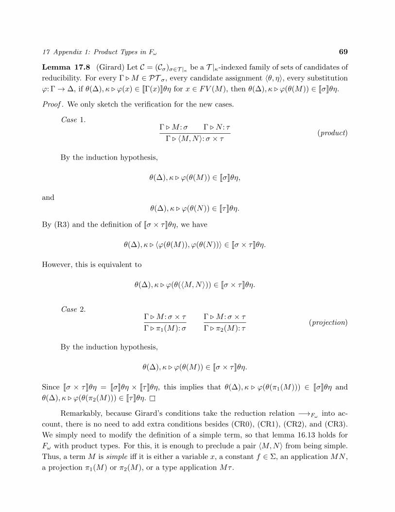
17 Appendix 1: Product Types in F! 69
Lemma 17.8 (Girard) Let C = (C�
)�2T | be a T |
-indexed family of sets of candidates of
reducibility. For every � .M 2 PT�
, every candidate assignment h✓, ⌘i, every substitution
':�! �, if ✓(�), . '(x) 2 [[�(x)]]✓⌘ for x 2 FV (M), then ✓(�), . '(✓(M)) 2 [[�]]✓⌘.
Proof . We only sketch the verification for the new cases.
Case 1.� .M :� � .N : ⌧
� . hM,Ni:� ⇥ ⌧(product)
By the induction hypothesis,
✓(�), . '(✓(M)) 2 [[�]]✓⌘,
and
✓(�), . '(✓(N)) 2 [[⌧ ]]✓⌘.
By (R3) and the definition of [[� ⇥ ⌧ ]]✓⌘, we have
✓(�), . h'(✓(M)),'(✓(N))i 2 [[� ⇥ ⌧ ]]✓⌘.
However, this is equivalent to
✓(�), . '(✓(hM,Ni)) 2 [[� ⇥ ⌧ ]]✓⌘.
Case 2.� .M :� ⇥ ⌧
� . ⇡1(M):�
� .M :� ⇥ ⌧
� . ⇡2(M): ⌧(projection)
By the induction hypothesis,
✓(�), . '(✓(M)) 2 [[� ⇥ ⌧ ]]✓⌘.
Since [[� ⇥ ⌧ ]]✓⌘ = [[�]]✓⌘ ⇥ [[⌧ ]]✓⌘, this implies that ✓(�), . '(✓(⇡1(M))) 2 [[�]]✓⌘ and
✓(�), . '(✓(⇡2(M))) 2 [[⌧ ]]✓⌘.
Remarkably, because Girard’s conditions take the reduction relation �!F! into ac-
count, there is no need to add extra conditions besides (CR0), (CR1), (CR2), and (CR3).
We simply need to modify the definition of a simple term, so that lemma 16.13 holds for
F!
with product types. For this, it is enough to preclude a pair hM,Ni from being simple.
Thus, a term M is simple i↵ it is either a variable x, a constant f 2 ⌃, an application MN ,
a projection ⇡1(M) or ⇡2(M), or a type application M⌧ .
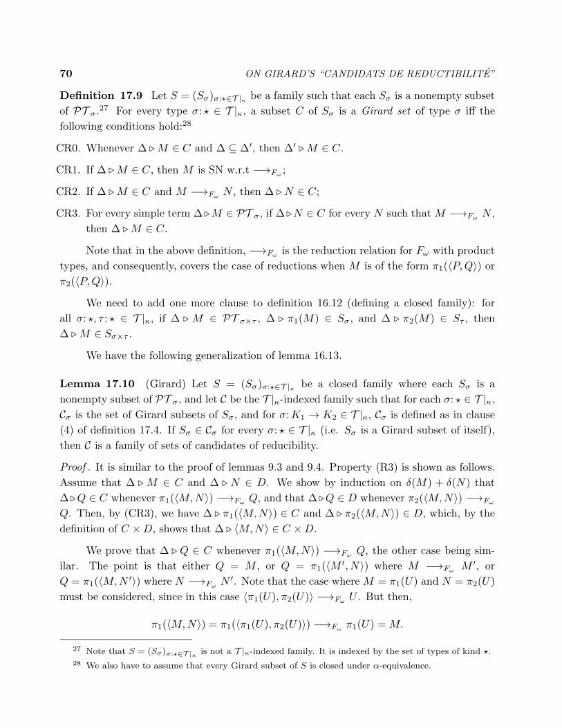
70 ON GIRARD’S “CANDIDATS DE REDUCTIBILITE”
Definition 17.9 Let S = (S�
)�:?2T | be a family such that each S
�
is a nonempty subset
of PT�
.27 For every type �: ? 2 T |
, a subset C of S�
is a Girard set of type � i↵ the
following conditions hold:28
CR0. Whenever � .M 2 C and � ✓ �0, then �0 .M 2 C.
CR1. If � .M 2 C, then M is SN w.r.t �!F! ;
CR2. If � .M 2 C and M �!F! N , then � .N 2 C;
CR3. For every simple term �.M 2 PT�
, if �.N 2 C for every N such that M �!F! N ,
then � .M 2 C.
Note that in the above definition, �!F! is the reduction relation for F
!
with product
types, and consequently, covers the case of reductions when M is of the form ⇡1(hP,Qi) or⇡2(hP,Qi).
We need to add one more clause to definition 16.12 (defining a closed family): for
all �: ?, ⌧ : ? 2 T |
, if � . M 2 PT�⇥⌧
, � . ⇡1(M) 2 S�
, and � . ⇡2(M) 2 S⌧
, then
� .M 2 S�⇥⌧
.
We have the following generalization of lemma 16.13.
Lemma 17.10 (Girard) Let S = (S�
)�:?2T | be a closed family where each S
�
is a
nonempty subset of PT�
, and let C be the T |
-indexed family such that for each �: ? 2 T |
,
C�
is the set of Girard subsets of S�
, and for �:K1 ! K2 2 T |
, C�
is defined as in clause
(4) of definition 17.4. If S�
2 C�
for every �: ? 2 T |
(i.e. S�
is a Girard subset of itself),
then C is a family of sets of candidates of reducibility.
Proof . It is similar to the proof of lemmas 9.3 and 9.4. Property (R3) is shown as follows.
Assume that � . M 2 C and � . N 2 D. We show by induction on �(M) + �(N) that
�.Q 2 C whenever ⇡1(hM,Ni) �!F! Q, and that �.Q 2 D whenever ⇡2(hM,Ni) �!
F!
Q. Then, by (CR3), we have � . ⇡1(hM,Ni) 2 C and � . ⇡2(hM,Ni) 2 D, which, by the
definition of C ⇥D, shows that � . hM,Ni 2 C ⇥D.
We prove that � . Q 2 C whenever ⇡1(hM,Ni) �!F! Q, the other case being sim-
ilar. The point is that either Q = M , or Q = ⇡1(hM 0, Ni) where M �!F! M 0, or
Q = ⇡1(hM,N 0i) where N �!F! N 0. Note that the case where M = ⇡1(U) and N = ⇡2(U)
must be considered, since in this case h⇡1(U),⇡2(U)i �!F! U . But then,
⇡1(hM,Ni) = ⇡1(h⇡1(U),⇡2(U)i) �!F! ⇡1(U) = M.
27 Note that S = (S�)�:?2T | is not a T |-indexed family. It is indexed by the set of types of kind ?.28 We also have to assume that every Girard subset of S is closed under ↵-equivalence.

17 Appendix 1: Product Types in F! 71
In the first case, the hypothesis yields � . M 2 C. In the other two cases, by (CR2) we
have � . M 0 2 C and � . N 0 2 D , and since �(M 0) < �(M) and �(N 0) < �(N), we use
the induction hypothesis and (CR3). The base case where M and N are irreducible follows
from (CR3).
It is also necessary to verify conditions (1), (2), (3), (4), (5) of definition 17.4. This is
done by induction on kinds, and for the kind ? by induction on types. The only new case is
case (5). Given that C ✓ S�
and D ✓ S⌧
, the fact that C⇥D ✓ S�⇥⌧
follows from the new
closure condition (on ⇥). We need to prove that (CR1), (CR2), and (CR3) hold for C ⇥D,
given that they hold for C and D. Let � .M :�⇥ ⌧ be a term in C ⇥D, where C 2 C�
and
D 2 C⌧
. By the definition of C ⇥D, � . ⇡1(M) 2 C (and � . ⇡2(M) 2 D). Since all terms
in C are SN, ⇡1(M) is SN. But then, M itself is necessary SN since any infinite reduction
from M yields an infinite reduction from ⇡1(M).
Assume that M �!F! M 0. Then, ⇡1(M) �!
F! ⇡1(M 0) and ⇡2(M) �!F! ⇡2(M 0).
Since ⇡1(M) 2 C and ⇡2(M) 2 D, by (CR2) applied to C and D, we have ⇡1(M 0) 2 C and
⇡2(M 0) 2 D. By the definition of C ⇥D, we have � .M 0 2 C ⇥D, and (CR2) holds.
Now, assume that M is simple, and that whenever M �!F! Q, then � .Q 2 C ⇥D.
We want to prove that � .M 2 C ⇥D. Note that ⇡1(M) and ⇡2(M) are also simple, and
that because M is simple,
(⇤) ⇡1(M) �!F! R implies that R = ⇡1(Q) where M �!
F! Q, and similarly for ⇡2(M).
Since we assumed that � . Q 2 C ⇥ D, we have � . ⇡1(Q) 2 C and � . ⇡2(Q) 2D. By (CR3) applied to C and D and (⇤), since ⇡1(M) and ⇡2(M) are simple, we have
� . ⇡1(M) 2 C and � . ⇡2(M) 2 D. By the definition of C ⇥D, we have � .M 2 C ⇥D,
and (CR3) holds.
We now have a version of Girard’s fundamental theorem for F!
with product types.
Theorem 17.11 (Girard) Let S = (S�
)�:?2T | be a closed family where each S
�
is a
nonempty subset of PT�
, let C be the T |
-indexed family of sets defined in lemma 17.10,
and assume that S�
2 C�
for every �: ? 2 T |
. For every �.M 2 PT�
, we have �.M 2 S�
.
Proof . By lemma 17.10, C is a family of sets of candidates of reducibility. We now apply
lemma 17.8 to any assignment (for example, the assignment with value ⌘(t) = cant
), the
identity type substitution, and the identity term substitution, which is legitimate since by
(CR3), every variable belongs to every Girard set.29
29 Actually, some ↵-renaming may have to be performed on M and � so that they are both safe for thetype and term identity substitution.

72 ON GIRARD’S “CANDIDATS DE REDUCTIBILITE”
The next lemma shows that F!
with product types is strongly normalizing and con-
fluent under both �-reduction and �⌘-reduction.
Lemma 17.12 (i) The family SN�
such that for every �: ? 2 T |
, SN�,�
is the set
of typing judgments � . M :� provable in F!
such that M is strongly normalizing under
�-reduction, is a closed family of Girard sets. (ii) The family SN�⌘
such that for every
�: ? 2 T |
, SN�⌘,�
is the set of typing judgments � .M :� provable in F!
such that M is
strongly normalizing under �⌘-reduction, is a closed family of Girard sets. (iii) The family
consisting for every �: ? 2 T |
of the set of typing judgments � .M :� provable in F!
such
that confluence under �-reduction holds from M and all of its subterms, is a closed family
of Girard sets. (iv) The family consisting for every �: ? 2 T |
of the set of typing judgments
� .M :� provable in F!
such that confluence under �⌘-reduction holds from M and all of
its subterms, is a closed family of Girard sets.
Proof . (i)-(ii) It is trivial to verify that closure and (CR0)–(CR3) hold. (iii)-(iv) The
proof is similar to the one given in appendix 2, with a few more cases involving pairs and
projections.
18 Appendix 2
This appendix contains the details that were omitted in the proof of lemma 10.2.
Proof of lemma 10.2. We need to prove that the family of sets in (iii) and (iv) is a closed
family of saturated sets.
Closure is obvious since if confluence holds from Mx and all of its subterms, then it
holds from M .
Verifying (S1) is easy and uses the fact that if confluence holds from N1, . . . , Nn
and
all of their subterms, then confluence holds from each uN1 . . . Nk
and all of its subterms,
where u 2 X [ ⌃ and 1 k n. This is because reductions must apply withing the Ni
’s.
Since confluence from u is trivial, confluence from each subterm of uN1 . . . Nn
follows from
the assumption on N1, . . . , Nn
.
Proving (S2) is very tedious. Assume that confluence holds from M [N/x]N1 . . . Nn
and all of its subterms (and that confluence holds from N , which is implied by (S2)).
Thus, confluence holds from M,N,N1, . . . , Nn
. We need to show that confluence holds
from (�x:�. M)NN1 . . . Nn
and all of its subterms.
First, we show confluence from every subterm of �x:�.M . Since confluence holds from
every subterm of M , the only nontrivial case is the case where M⇤�!
�
8 (M 01x), for some

18 Appendix 2 73
term M 01 such that x /2 FV (M 0
1). In this case, we can have reductions of the form
�x:�. M⇤�!
�
8 �x:�. (M 01x) �!⌘
M 01
⇤�!�
8 P1,
where M⇤�!
�
8 M 01x. There are four cases to consider.
Case 1.
�x:�. M⇤�!
�
8 �x:�. (M 01x) �!⌘
M 01
⇤�!�
8 P1
and
�x:�. M⇤�!
�
8 �x:�. (M 001 x) �!⌘
M 001
⇤�!�
8 P2,
where M⇤�!
�
8 M 01x and M
⇤�!�
8 M 001 x. Since confluence holds from M , there are reduc-
tions P1x⇤�!
�
8 Q and P2x⇤�!
�
8 Q for some Q.
If both reductions are of the form P1x⇤�!
�
8 P3x and P2x⇤�!
�
8 P3x, for some P3
such that Q = P3x, P1⇤�!
�
8 P3, and P2⇤�!
�
8 P3, then confluence holds.
If P2⇤�!
�
8 P3 and P1x⇤�!
�
8 P3x is of the form
P1x⇤�!
�
8 (�y:�. Q1)x �!�
Q1[x/y]⇤�!
�
8 P3x,
since x /2 FV (M 001 ) due to the ⌘-step, and since �y:�. Q1 ⌘↵
�x:�. Q1[x/y], we have
x /2 FV (P3) and
P1⇤�!
�
8 �y:�. Q1⇤�!
�
8 �x:�. (P3x) �!⌘
P3.
Confluence holds, since P2⇤�!
�
8 P3.
The subcase where P1⇤�!
�
8 P3 and
P2x⇤�!
�
8 (�y:�. Q2)x �!�
Q2[x/y]⇤�!
�
8 P3x,
is symmetric.
If both
P1x⇤�!
�
8 (�y:�. Q1)x �!�
Q1[x/y]⇤�!
�
8 Q,
and
P2x⇤�!
�
8 (�y:�. Q2)x �!�
Q2[x/y]⇤�!
�
8 Q,
since �y:�. Q1 ⌘↵
�x:�. Q1[x/y] and �y:�. Q2 ⌘↵
�x:�. Q2[x/y], we have
P1⇤�!
�
8 �y:�. Q1⇤�!
�
8 �x:�. Q
and
P2⇤�!
�
8 �y:�. Q2⇤�!
�
8 �x:�. Q.
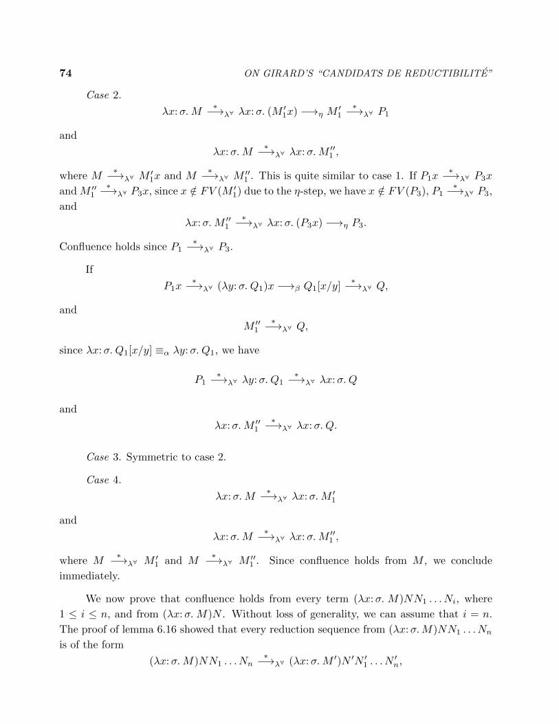
74 ON GIRARD’S “CANDIDATS DE REDUCTIBILITE”
Case 2.
�x:�. M⇤�!
�
8 �x:�. (M 01x) �!⌘
M 01
⇤�!�
8 P1
and
�x:�. M⇤�!
�
8 �x:�. M 001 ,
where M⇤�!
�
8 M 01x and M
⇤�!�
8 M 001 . This is quite similar to case 1. If P1x
⇤�!�
8 P3x
andM 001
⇤�!�
8 P3x, since x /2 FV (M 01) due to the ⌘-step, we have x /2 FV (P3), P1
⇤�!�
8 P3,
and
�x:�. M 001
⇤�!�
8 �x:�. (P3x) �!⌘
P3.
Confluence holds since P1⇤�!
�
8 P3.
If
P1x⇤�!
�
8 (�y:�. Q1)x �!�
Q1[x/y]⇤�!
�
8 Q,
and
M 001
⇤�!�
8 Q,
since �x:�. Q1[x/y] ⌘↵
�y:�. Q1, we have
P1⇤�!
�
8 �y:�. Q1⇤�!
�
8 �x:�. Q
and
�x:�. M 001
⇤�!�
8 �x:�. Q.
Case 3. Symmetric to case 2.
Case 4.
�x:�. M⇤�!
�
8 �x:�. M 01
and
�x:�. M⇤�!
�
8 �x:�. M 001 ,
where M⇤�!
�
8 M 01 and M
⇤�!�
8 M 001 . Since confluence holds from M , we conclude
immediately.
We now prove that confluence holds from every term (�x:�. M)NN1 . . . Ni
, where
1 i n, and from (�x:�. M)N . Without loss of generality, we can assume that i = n.
The proof of lemma 6.16 showed that every reduction sequence from (�x:�.M)NN1 . . . Nn
is of the form
(�x:�. M)NN1 . . . Nn
⇤�!�
8 (�x:�. M 0)N 0N 01 . . . N
0n
,

18 Appendix 2 75
or
(�x:�. M)NN1 . . . Nn
⇤�!�
8 (�x:�. M 0)N 0N 01 . . . N
0n
�!�
M 0[N 0/x]N 01 . . . N
0n
⇤�!�
8 Q,
or
(�x:�. M)NN1 . . . Nn
⇤�!�
8 (�x:�. (M 01x))N
0N 01 . . . N
0n
�!⌘
M 01N
0N 01 . . . N
0n
⇤�!�
8 Q,
where in (1)-(2) M⇤�!
�
8 M 0, in (3) M⇤�!
�
8 M 01x, and in all cases N
⇤�!�
8 N 0, and
Ni
⇤�!�
8 N 0i
, for every i, 1 i n. We have seven main cases.
Case 1.
(�x:�. M)NN1 . . . Nn
⇤�!�
8 (�x:�. M 0)N 0N 01 . . . N
0n
and
(�x:�. M)NN1 . . . Nn
⇤�!�
8 (�x:�. M 00)N 00N 001 . . . N 00
n
.
Since confluence holds from M,N,N1 . . . Nn
(for N , this is implied by (S2)), we have re-
duction sequences M 0 ⇤�!�
8 M 000, M 00 ⇤�!�
8 M 000, N 0 ⇤�!�
8 N 000, N 00 ⇤�!�
8 N 000, and
N 0i
⇤�!�
8 N 000i
, N 00i
⇤�!�
8 N 000i
, for every i, 1 i n, and thus reductions
(�x:�. M 0)N 0N 01 . . . N
0n
⇤�!�
8 (�x:�. M 000)N 000N 0001 . . . N 000
n
and
(�x:�. M 00)N 00N 001 . . . N 00
n
⇤�!�
8 (�x:�. M 000)N 000N 0001 . . . N 000
n
.
Case 2.
(�x:�. M)NN1 . . . Nn
⇤�!�
8 (�x:�. M 0)N 0N 01 . . . N
0n
and
(�x:�. M)NN1 . . . Nn
⇤�!�
8 (�x:�. M 00)N 00N 001 . . . N 00
n
�!�
M 00[N 00/x]N 001 . . . N 00
n
⇤�!�
8 P2.
This time, we also have reduction sequences
(�x:�. M)NN1 . . . Nn
�!�
M [N/x]N1 . . . Nn
⇤�!�
8 M 0[N 0/x]N 01 . . . N
0n
and
(�x:�. M)NN1 . . . Nn
�!�
M [N/x]N1 . . . Nn
⇤�!�
8 M 00[N 00/x]N 001 . . . N 00
n
⇤�!�
8 P2.
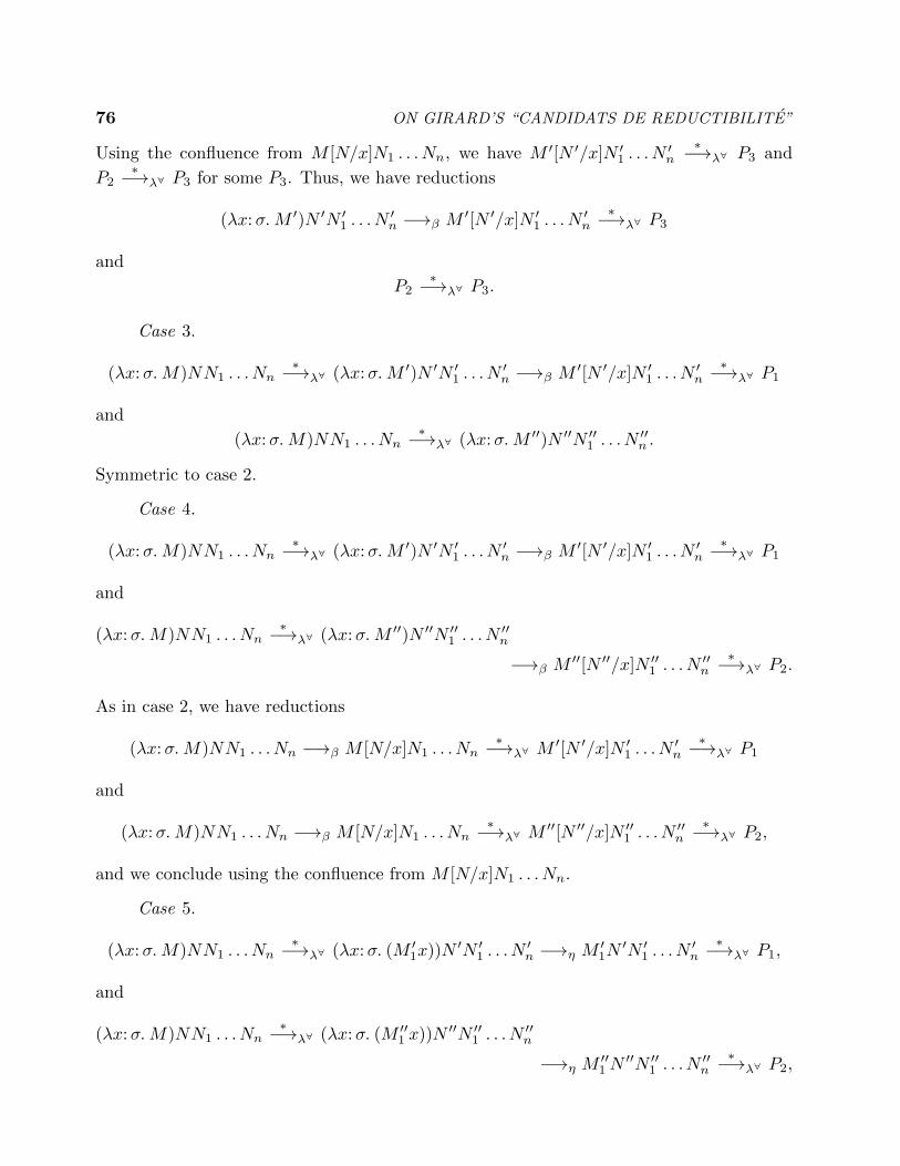
76 ON GIRARD’S “CANDIDATS DE REDUCTIBILITE”
Using the confluence from M [N/x]N1 . . . Nn
, we have M 0[N 0/x]N 01 . . . N
0n
⇤�!�
8 P3 and
P2⇤�!
�
8 P3 for some P3. Thus, we have reductions
(�x:�. M 0)N 0N 01 . . . N
0n
�!�
M 0[N 0/x]N 01 . . . N
0n
⇤�!�
8 P3
and
P2⇤�!
�
8 P3.
Case 3.
(�x:�. M)NN1 . . . Nn
⇤�!�
8 (�x:�. M 0)N 0N 01 . . . N
0n
�!�
M 0[N 0/x]N 01 . . . N
0n
⇤�!�
8 P1
and
(�x:�. M)NN1 . . . Nn
⇤�!�
8 (�x:�. M 00)N 00N 001 . . . N 00
n
.
Symmetric to case 2.
Case 4.
(�x:�. M)NN1 . . . Nn
⇤�!�
8 (�x:�. M 0)N 0N 01 . . . N
0n
�!�
M 0[N 0/x]N 01 . . . N
0n
⇤�!�
8 P1
and
(�x:�. M)NN1 . . . Nn
⇤�!�
8 (�x:�. M 00)N 00N 001 . . . N 00
n
�!�
M 00[N 00/x]N 001 . . . N 00
n
⇤�!�
8 P2.
As in case 2, we have reductions
(�x:�. M)NN1 . . . Nn
�!�
M [N/x]N1 . . . Nn
⇤�!�
8 M 0[N 0/x]N 01 . . . N
0n
⇤�!�
8 P1
and
(�x:�. M)NN1 . . . Nn
�!�
M [N/x]N1 . . . Nn
⇤�!�
8 M 00[N 00/x]N 001 . . . N 00
n
⇤�!�
8 P2,
and we conclude using the confluence from M [N/x]N1 . . . Nn
.
Case 5.
(�x:�. M)NN1 . . . Nn
⇤�!�
8 (�x:�. (M 01x))N
0N 01 . . . N
0n
�!⌘
M 01N
0N 01 . . . N
0n
⇤�!�
8 P1,
and
(�x:�. M)NN1 . . . Nn
⇤�!�
8 (�x:�. (M 001 x))N
00N 001 . . . N 00
n
�!⌘
M 001 N
00N 001 . . . N 00
n
⇤�!�
8 P2,

18 Appendix 2 77
where M⇤�!
�
8 M 01x, M
⇤�!�
8 M 001 x. Because of the ⌘-steps, x /2 FV (M 0
1) and x /2FV (M 00
1 ), and thus M 01[N
0/x] = M 01 and M 00
1 [N00/x] = M 00
1 , and we have reductions
(�x:�. M)NN1 . . . Nn
�!�
M [N/x]N1 . . . Nn
⇤�!�
8 M 01N
0N 01 . . . N
0n
⇤�!�
8 P1,
and
(�x:�. M)NN1 . . . Nn
�!�
M [N/x]N1 . . . Nn
⇤�!�
8 M 001 N
00N 001 . . . N 00
n
⇤�!�
8 P2,
and we conclude using the confluence from M [N/x]N1 . . . Nn
.
Case 6.
(�x:�. M)NN1 . . . Nn
⇤�!�
8 (�x:�. (M 01x))N
0N 01 . . . N
0n
�!⌘
M 01N
0N 01 . . . N
0n
⇤�!�
8 P1,
and
(�x:�. M)NN1 . . . Nn
⇤�!�
8 (�x:�. M 001 N
00)N 001 . . . N 00
n
�!�
M 001 [N
00/x]N 001 . . . N 00
n
⇤�!�
8 P2,
where M⇤�!
�
8 M 01x, M
⇤�!�
8 M 001 . Since we have an ⌘-reduction step, x /2 FV (M 0
1),
which implies that M 01[N
0/x] = M 01, and we have
(�x:�. M)NN1 . . . Nn
�!�
M [N/x]N1 . . . Nn
⇤�!�
8 M 01N
0N 01 . . . N
0n
⇤�!�
8 P1,
and
(�x:�. M)NN1 . . . Nn
⇤�!�
M [N/x]N1 . . . Nn
⇤�!�
8 M 001 [N
00/x]N 001 . . . N 00
n
⇤�!�
8 P2.
We conclude using the confluence from M [N/x]N1 . . . Nn
.
Case 7. Symmetric to case 6.
Proving that confluence holds from (⇤t. M)⌧N1 . . . Nn
and all its subterms assuming
that confluence holds from M [⌧/t]N1 . . . Nn
and all its subterms is similar to the previous
proof, except that there are no reductions from ⌧ .

78 ON GIRARD’S “CANDIDATS DE REDUCTIBILITE”
19 References
[1] Barendregt, H. The Lambda Calculus. Its Syntax and Semantics, Revised Edition,
North-Holland, Amsterdam, 1984.
[2] Breazu-Tannen, V., and Coquand, Th., Extensional models for polymorphism, Theor.
Comput. Sci. 59(1,2), 1988, 85-114.
[3] Breazu-Tannen, V., Combining Algebra and Higher-Order Types, In 3rd Annual Sym-
posium on Logic In Computer Science, IEEE Computer Society, Edinburgh, Scotland,
July 1988, 82-90.
[4] Breazu-Tannen, V., and Gallier, J.H., Polymorphic Rewriting Conserves Algebraic
Strong Normalization and Confluence, 16th International Colloquium on Automata,
Languages and Programming, ed. by G. Ausiello, M. Dezani-Ciancaglini, and S.
Ronchi Della Rocca, LNCS No. 372, Springer Verlag, July 1989, 137-150.
[5] Coquand, Th., Une Theorie des Constructions, These de 3eme Cycle, Universite de
Paris VII (1985).
[6] Coquand, Th., and Huet, G., The Calculus of Constructions, Information and Com-
putation 76(2/3), 1988, 95-120.
[7] Coquand, Th. Mathematical investigation of a calculus of constructions, In: Logic
and Computer Science, P. Odifreddi, editor, 1990.
[8] Fortune, S., Leivant, D., and O’Donnell, M., The expressiveness of simple and second-
order type structures, J.ACM 30(1), 1983, 151-185.
[9] Girard, J.Y., Une extension de l’interpretation de Godel a l’analyse, et son application
a l’elimination des coupures dans l’analyse et la theorie des types, Proc. 2nd Scand.
Log. Symp., 1970, ed. J.E. Fenstad, North-Holland, Amsterdam, 1971, 63-92.
[10] Girard, J.Y., Interpretation functionelle et elimination des coupures de l’arithmetique
d’ordre superieur, These d’Etat, Universite de Paris VII (1972).
[11] Girard, J.Y., Lafont, Y., and Taylor, P., Proofs and Types, Cambridge University
Press, 1989.
[12] Girard, J.Y., Proof Theory and Logical Complexity, Studies in proof theory, Bib-
liopolis, Napoli, 1987.
[13] Harper, R., Honsell, F., and Plotkin, G., A Framework for Defining Logics, In 2nd
Annual Symposium on Logic In Computer Science, IEEE Computer Society, Ithaca,
New York, June 1987, 194-204.
19 References 79
[14] Harper, R., Honsell, F., and Plotkin, G., A Framework for Defining Logics, draft sub-
mitted for publication, Department of Computer Science, Carnegie Mellon University,
Pittsburgh, PA 15213, 1989.
[15] Hindley, J.R., and Seldin, J.P., Introduction to Combinators and Lambda Calculus,
Cambridge University Press, 1986.
[16] Huet, G., Resolution d’Equations dans les Langages d’Ordre 1, 2, . . . ,!, These d’Etat,
Universite de Paris VII (1976).
[17] Huet, G., “Confluent Reductions: Abstract Properties and Applications to Term
Rewriting Systems,” J.ACM 27:4, 1980, 797-821.
[18] Huet, G., Deduction and Computation, Lecture Notes, Department of Computer
Science, Carnegie Mellon University, Pittsburgh, PA 15213, 1987.
[19] Lambek, J., and Scott, P.J., Introduction to Higher Order Categorical Logic, Cam-
bridge University Press, 1986.
[20] Leivant, D., Typing and Computational Properties of Lambda Expressions, Theoret-
ical Computer Science 44, 1986, 51-68.
[21] Martin-Lof, P., Hauptsatz for the Intuitionistic Theory of Iterated Inductive Defi-
nitions, Proc. 2nd Scand. Log. Symp., 1970, ed. J.E. Fenstad, North-Holland,
Amsterdam, 1971, 179-216.
[22] Martin-Lof, P., Hauptsatz for the Theory of Species, Proc. 2nd Scand. Log. Symp.,
1970, ed. J.E. Fenstad, North-Holland, Amsterdam, 1971, 217-233.
[23] Martin-Lof, P., Hauptsatz for Intuitionistic Simple Type Theory, In Logic, Method-
ology and Philosophy of Science IV, ed. by P. Suppes, L. Henkin, A. Joja, and Gr.C.
Moisil, North-Holland, Amsterdam, 1973, 279-290.
[24] Mitchell, J.C., A type-inference approach to reduction properties and semantics of
polymorphic expressions, In Proc. 1986 ACM Symposium on Lisp and Functional
Programming, ACM, New York, August 1986, 308-319.
[25] Mitchell, J.C., Type Systems for Programming Languages, to appear in Handbook
of Theoretical Computer Science, ed. by J. van Leeuwen, A. Meyer, and D. Perrin,
North-Holland, 1990.
[26] Paulin-Morhing, C., Extraction de programmes dans le calcul des constructions, These
d’Etat, Universite de Paris VII, 1989.
19 References 81
[40] de Vrijer, R.C., Exactly estimating functionals and strong normalization, Proceedings
of the Koninklijke Nederlandse Akademie van Wetenschappen, Series A, Volume 90,
No. 4, December 18, 1987, 479-493.

80 ON GIRARD’S “CANDIDATS DE REDUCTIBILITE”
[27] Pfenning, F., Partial Polymorphic Type Inference and Higher-Order Unification, In
1988 ACM Conference on Lisp and Functional Programming, ACM, Snowbird, Utah,
July 25-27, 1988, 153-163.
[28] Pfenning, F., Elf, A language for logic definition and verified metaprogramming, In 4th
Annual Symposium on Logic In Computer Science, IEEE Computer Society, Asilomar,
California, June 1989, 313-322.
[29] Prawitz, D., Ideas and Results in Proof Theory, Proc. 2nd Scand. Log. Symp., 1970,
ed. J.E. Fenstad, North-Holland, Amsterdam, 1971, 235-307.
[30] Reynolds, J., Towards a theory of type structure. In Proc. sur la Programmation,
LCNS No. 19, Springer Verlag, NY, 1974, 408-425.
[31] Scedrov, A, Normalization revisited, In: Categories in Logic and Computer Science,
Proceedings of a Summer Research Conference, Boulder, Colorado, June 1987, ed. by
J.W. Gray and A. Scedrov, Contemporary Mathematics, Vol. 92, Amer. Math. Soc.,
Providence, RI, 1989, 357-369.
[32] Scedrov, A., A guide to polymorphic types, In: Logic and Computer Science, P.
Odifreddi, editor, 1990.
[33] Seldin, J.P., Mathesis: The Mathematical Foundations of Ulysses, Technical Report
RADC-TR-87-223, Odyssey Research Associates, 1987.
[34] Statman, R., Logical Relations and the Typed �-Calculus, Information and Control
65, 3-2, 1985, 85-97.
[35] Stenlund, S., Combinators, Lambda Terms, and Proof Theory, D. Reidel, Dordrecht,
Holland, 1972.
[36] Tait, W.W., Intensional interpretation of functionals of finite type I, J. Symbolic Logic
32, 1967, 198-212.
[37] Tait, W.W., A realizability interpretation of the theory of species, In Logic Collo-
quium, ed. R. Parikh, LNCS No. 453, Springer Verlag, 1975, 240-251.
[38] de Vrijer, R.C., Surjective Pairing and Strong Normalization: Two Themes in Lambda
Calculus, Doctoral thesis, Amsterdam, the Netherlands, 1987.
[39] de Vrijer, R.C., Strong Normalization in N -HA!
p
, Proceedings of the Koninklijke
Nederlandse Akademie van Wetenschappen, Series A, Volume 90, No. 4, December
18, 1987, 473-478.