Technical ReportDoc ID: TR-1-2013

06-March-2013(Last revision: 23-February-2016)

On formulating quadraticfunctions in optimizationmodels.

Author: Erling D. Andersen

Convex quadratic constraints quite frequently appear in optimization problems andhence it is important to know how to formulate them efficiently. In this note it isargued that reformulating them to separable form is advantageous because it makes theconvexity check trivial and usually leads to a faster solution time requiring less storage.The suggested technique is particularly applicable in portfolio optimization where afactor model for the covariance matrix is employed.

Moreover, we discuss how to formulate quadratic constraints using quadratic conesand the benefits of doing that.

1 Introduction

Consider the quadratic optimization problem

minimize cTxsubject to 1

2xTQx+ aTx+ b ≤ 0

(1)

where Q is symmetricQ = QT .

Normally there are some structure in the Q matrix e.g. Q may be a low rank matrix or have a factorstructure. The problem (1) is said to be separable if Q is a diagonal matrix. Subsequently it isdemonstrated how the problem (1) always can be reformulated to have a separable structure.

For simplicity it is assumed that the problem (1) only has one constraint. However, it should beobvious how to extend the suggested techniques to a problem with an arbitrary number of constraints.Moreover, it is important to note that the techniques outlined are applicable to problems with aquadratic objective as well. Indeed the problem

minimize cTx+ 12x

TQx (2)

is equivalent tominimize cTx+ tsubject to 1

2xTQx ≤ t

(3)

which has the form (1).

2 The convexity assumption

The problem (1) is an easy problem to solve if it is a convex problem. It is well known that theproblem (1) is convex if and only if the quadratic function

f(x) = xTQx (4)

is convex. Furthermore, the following statements are equivalent.

www.mosek.com Page 1 of 6

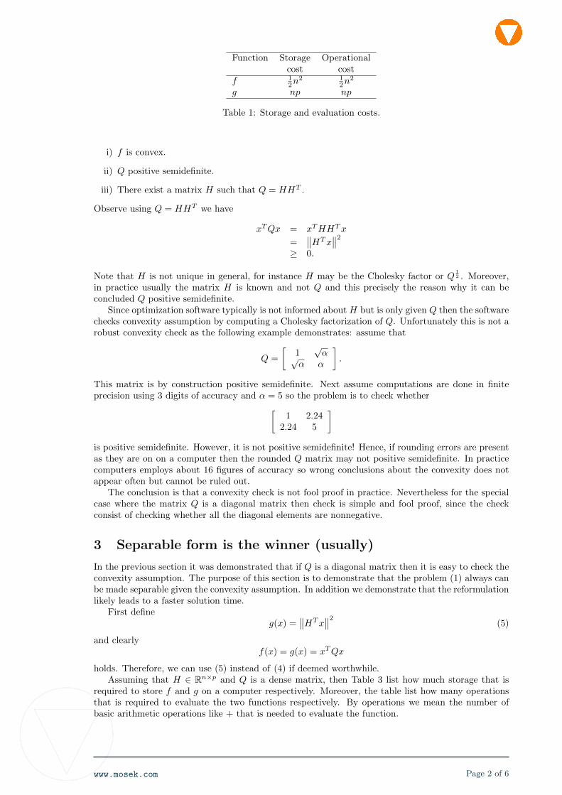
Function Storage Operationalcost cost

f 12n

2 12n

2

g np np

Table 1: Storage and evaluation costs.

i) f is convex.

ii) Q positive semidefinite.

iii) There exist a matrix H such that Q = HHT .

Observe using Q = HHT we have

xTQx = xTHHTx

=∥∥HTx

∥∥2≥ 0.

Note that H is not unique in general, for instance H may be the Cholesky factor or Q12 . Moreover,

in practice usually the matrix H is known and not Q and this precisely the reason why it can beconcluded Q positive semidefinite.

Since optimization software typically is not informed about H but is only given Q then the softwarechecks convexity assumption by computing a Cholesky factorization of Q. Unfortunately this is not arobust convexity check as the following example demonstrates: assume that

Q =

[1√α√

α α

].

This matrix is by construction positive semidefinite. Next assume computations are done in finiteprecision using 3 digits of accuracy and α = 5 so the problem is to check whether[

1 2.242.24 5

]is positive semidefinite. However, it is not positive semidefinite! Hence, if rounding errors are presentas they are on on a computer then the rounded Q matrix may not positive semidefinite. In practicecomputers employs about 16 figures of accuracy so wrong conclusions about the convexity does notappear often but cannot be ruled out.

The conclusion is that a convexity check is not fool proof in practice. Nevertheless for the specialcase where the matrix Q is a diagonal matrix then check is simple and fool proof, since the checkconsist of checking whether all the diagonal elements are nonnegative.

3 Separable form is the winner (usually)

In the previous section it was demonstrated that if Q is a diagonal matrix then it is easy to check theconvexity assumption. The purpose of this section is to demonstrate that the problem (1) always canbe made separable given the convexity assumption. In addition we demonstrate that the reformulationlikely leads to a faster solution time.

First defineg(x) =

∥∥HTx∥∥2 (5)

and clearlyf(x) = g(x) = xTQx

holds. Therefore, we can use (5) instead of (4) if deemed worthwhile.Assuming that H ∈ Rn×p and Q is a dense matrix, then Table 3 list how much storage that is

required to store f and g on a computer respectively. Moreover, the table list how many operationsthat is required to evaluate the two functions respectively. By operations we mean the number ofbasic arithmetic operations like + that is needed to evaluate the function.

www.mosek.com Page 2 of 6

Table 3 shows that if p is much smaller than n, then using the formulation (5) saves a huge amountof storage and work. This observation can be used to reformulate (1) to

minimize cTxsubject to 1

2yT y + aTx+ b ≤ 0,

HTx− y = 0.(6)

The formulation (6) is larger than (1) because p additional linear equalities and variables havebeen added. However, if p is much smaller than n, then the formulation (6) requires much less storagewhich in most cases leads to a much faster solution times.

Before continuing then let us take a look at an important special case. Assume a vector v is knownsuch that

Hv = a

For instance if H is nonsingular, then v exists and can be computed as H−1a. It many practicalapplications a v will be trivially known.

Now if we letHTx− y = −v

then‖y‖2 =

∥∥HTx+ v∥∥2

= xTHHTx+ vT v + 2xTHv= xTQx+ 2aTx+ vT v

Therefore, problem (6) and

minimize cTxsubject to 0.5yT y − 0.5vT v + b ≤ 0,

HTx− y = v.(7)

is equivalent. The reformulation (7) is sparser than (6) in the constraint matrix because the problemno longer contains a and may therefore be preferable.

Now let us consider a slight generalization i.e. let us assume that

Q = D +HHT (8)

where D is positive semidefinite matrix. This implies Q is positive semidefinite. Furthermore, D isassumed to be simple e.g. a diagonal matrix. Using the structure in (8) then (1) can be cast as

minimize cTxsubject to 1

2 (xTDx+ yT y) + aTx+ b ≤ 0,HTx− y = 0.

(9)

In portfolio optimization arising in finance n may be 1000 and p is less than, say 50. In that case (9)will require about 10 times less storage compared to (1) assuming Q is dense. This will translate intodramatic faster solution times.

4 Conic reformulation

It is always possible and often worthwhile to reformulate convex quadratic and quadratically con-strained optimization problems on conic form. In this section we will discuss that possibility.

We will use the definitionsKq := {x ∈ Rn | x1 ≥ ‖x2:n‖}

andKr := {x ∈ Rn | 2x1x2 ≥ ‖x3:n‖2 , x1, x2 ≥ 0}.

Hence, Kq is the quadratic cone and Kr is the rotated quadratic cone.Let us first consider the conic reformulation of (6) which is

minimize cTxsubject to t+ aTx+ b = 0,

HTx− y = −h,s = 1, s

ty

∈ Kr.

(10)

www.mosek.com Page 3 of 6

or more compactlyminimize cTxsubject to t+ aTx+ b = 0, 1

tHTx+ h

∈ Kr.(11)

Next consider (7) which is infeasible if

0.5vT v − b < 0.

Now assume that is not the case then (7) can be stated on the form

minimize cTxsubject to HTx− y = −v,

t =√

0.5vT v − b,[ty

]∈ Kq

(12)

or compactlyminimize cTx

subject to

[ √0.5vT v − bHTx+ v

]∈ Kq.

(13)

Next let us consider the problem (9) which can be reformulated as a conic quadratic optimization

problem as follows. First we scale the x variable by D− 12 i.e. we replace x by D− 1

2 x to obtain

minimize cTD− 12x

subject to 12 (xTx+ yT y) + aTx+ b ≤ 0,

HTD− 12x− y = 0.

(14)

which equivalent to the conic quadratic problem

minimize cTD− 12 x

subject to t+ aTD− 12 x+ b = 0,

HTD− 12 x− y = 0,

1txy

∈ Kr.

(15)

When the optimal solution to (15) is computed then original solution can obtained from

x = D− 12 x.

5 Linear least squares problems with inequalities

An example of generalized linear least square problem is

minimize∥∥HTx+ h

∥∥subject to Ax ≥ b.

(16)

Here we will discuss how to reformulate that as a conic optimization problem.The problem (16) can be seen as a quadratic optimization problem because minimizing∥∥HTx+ h

∥∥or ∥∥HTx+ h

∥∥2 = xTHHTx+ 2hTHx+ hTh

is equivalent. Therefore, the problem (16) may be stated as the quadratic optimization problem

minimize xTHHTx+ 2hTHx+ hThsubject to Ax ≥ b.

(17)

www.mosek.com Page 4 of 6

The conic quadratic reformulation of (16) is trivial because it is

minimize tsubject to Ax ≥ b,[

tHTx+ h

]∈ Kq.

(18)

whereas the conic reformulation of (17) is

minimize t+ 2hTHx+ hThsubject to Ax ≥ b, 0.5

tHTx

∈ Kr.(19)

Now the question is should (18) or (19) be preferred? Consider the following problem

minimize ‖x‖subject to

∑nj=1 xj ≥ α,

x ≥ 0.(20)

For n = 10 and α = 104, then MOSEK version 7 requires 22 iterations to solve (19) whereas only6 iterations are required to solve the formulation (18) where the accuracy of the reported solution isabout the same in both cases. If α is reduced to 1 the two methods formulation are equally good interms of the number iterations. This confirms our experience that the formulation (18) usually leadsto the best results. The reason for this is might be that the norm is a nicer function than the squarednorm in the sense that the norm of something is closer to one than the squared norm.

We therefore offer the advice that a least square objective as in (16) is not converted to a quadraticproblem which then is converted to a conic problem. Rather it should directly be stated on its naturalconic quadratic form (18).

6 On the numerical benefits of a conic reformulation

In this section we will demonstrate that a conic reformulation of quadratic constraint often leads to abetter scaling.

Consider the quadratic constraintsxTx ≤ 10−12

andxTx ≤ 1012.

The conic reformulations aret = 10−6,[

tx

]∈ Kq

andt = 106,[

tx

]∈ Kq.

respectively. Observe, the numbers appearing in the conic reformulation is much closer to one andhence the problems are much better scaled.

Next consider the quadratic constraint

10−2x21 + 10−4x22 + 10−8x23 ≤ 10−8

which has the conic quadratic reformulation

t = 10−4,y1 = 10−1x1,y2 = 10−3x2,y3 = 10−4x3,[ty

]∈ Kq

www.mosek.com Page 5 of 6

Observe that the conic reformulation is better scaled. Indeed the relative difference between thebiggest and smallest number is reduced by 3 orders of magnitude by doing the conic reformulation.

Finally, we may use the substitutiony = 10−2y

to obtaint = 10−2,y1 = 101x1,y2 = 10−1x2,y3 = 10−2x3,[ty

]∈ Kq

which improves the scaling further.Clearly, the conic reformulation is bigger because there are more variables and hence may take

longer time to solve. However, the additional constraints and variables are very sparse and normallythis means only slightly higher computational costs per iteration. On other the reformulation maylead to fewer so in many cases the solution time will be shorter after reformulation.

7 Conclusion

In this note we have showed that when a quadratic function occur in an optimization problem thenthere might be different ways of representing them. Moreover, given a suitable structure in thequadratic term then a reformulation to separable form may lead to much more effective representation.In addition the reformulation leads to a much simpler and fool proof convexity check.

Finally, we have discussed how to formulate quadratic constraints using quadratic cones. In par-ticular we argued when a least least square objective or least squares type constraints occur then theyshould not be converted to quadratic form and then converted to conic form. Rather the least squareterms should be represented naturally in conic framework without squaring the term.

www.mosek.com Page 6 of 6

Mosek ApS

Fruebjergvej 32100 CopenhagenDenmark

www.mosek.com

info@mosek.com

“the fast path to optimum”

MOSEK ApS provides optimization software which help our clientsto make better decisions. Our customer base consists of financial in-stitutions and companies, engineering and software vendors, amongothers.

The company was established in 1997 by Erling D. Andersen andKnud D. Andersen and it specializes in creating advanced softwarefor solution of mathematical optimization problems. In particular,the company focuses on solution of large-scale linear, quadratic, andconic optimization problems.