On Evolutionary Approaches to Wind Turbine Placementwith Geo-Constraints

Daniel LückeheDepartment of Geoinformation

Jade University of AppliedSciences

Oldenburg, Germanydaniel.lueckehe

@uni-oldenburg.de

Markus WagnerOptimisation and Logistics

University of AdelaideAdelaide, Australiamarkus.wagner

@adelaide.edu.au

Oliver KramerDepartment of Computing

ScienceUniversity of OldenburgOldenburg, Germany

oliver.kramer@uni-oldenburg.de

ABSTRACTWind turbine placement, i.e., the geographical planning ofwind turbine locations, is an important first step to an ef-ficient integration of wind energy. The turbine placementproblem becomes a difficult optimization problem due tovarying wind distributions at different locations and due tothe mutual interference in the wind field known as wakeeffect. Artificial and environmental geological constraintsmake the optimization problem even more difficult to solve.In our paper, we focus on the evolutionary turbine placementbased on an enhanced wake effect model fed with real-worldwind distributions. We model geo-constraints with real-world data from OpenStreetMap. Besides the realistic mod-eling of wakes and geo-constraints, the focus of the paperis on the comparison of various evolutionary optimizationapproaches. We propose four variants of evolution strate-gies with turbine-oriented mutation operators and compareto state-of-the-art optimizers like the CMA-ES in a detailedexperimental analysis on three benchmark scenarios.

Categories and Subject DescriptorsG.1.6 [Optimization]: Constrained optimization; I.2.8[Artificial Intelligence]: Problem Solving, Control Meth-ods, and Search

KeywordsWind Power, Wind Farm Layout, Evolutionary Optimiza-tion, Self-Adaptation, CMA-ES

1. INTRODUCTIONRenewable energy plays an increasing role in the energy

supply world-wide. The integration of geo-information intoplanning processes becomes more and more important, re-sulting in a complex geo-planning problem with many con-straints. In particular, the effective integration of wind en-

Permission to make digital or hard copies of all or part of this work for personal orclassroom use is granted without fee provided that copies are not made or distributedfor profit or commercial advantage and that copies bear this notice and the full cita-tion on the first page. Copyrights for components of this work owned by others thanACM must be honored. Abstracting with credit is permitted. To copy otherwise, or re-publish, to post on servers or to redistribute to lists, requires prior specific permissionand/or a fee. Request permissions from permissions@acm.org.

GECCO ’15, July 11 - 15, 2015, Madrid, Spainc© 2015 ACM. ISBN 978-1-4503-3472-3/15/07. . . $15.00

DOI: http://dx.doi.org/10.1145/2739480.2754690

ergy is significantly influenced by the locations of wind tur-bines. Wind turbine placement optimization is the processof determining the placement of wind turbines within a spec-ified land or offshore area, such that the output power ofthe wind farm is maximized. An optimized placement re-sult allows wind farm installations to maximize their cost-effectiveness, thereby increasing their competitiveness in theenergy market. However, the optimal placement of wind tur-bines considering geo-constraints is a complex optimizationproblem that is hard to solve by exact methods. The solu-tion space is non-linear with respect to how sited turbinesinteract when considering wake loss and energy capture, inparticular when facing constraints. In this paper, we em-ploy evolutionary heuristics to solve the turbine placementproblem.

Objective of this paper is to model a realistic wind turbineplacement scenario by taking into account realistic wake ef-fects, real-world wind data from a meteorological service,and geo-constraints from a topological map service. On thebasis of this model, we define three benchmark scenariosand analyze turbine-oriented heuristics while comparing tostate-of-the-art optimization algorithms like the covariancematrix adaptation evolution strategy (CMA-ES).

This paper is structured as follows. In Section 2, wepresent related work on turbine placement with evolutionaryalgorithms. Our enhanced wind model based on COSMO-DE data and Kusiak and Song’s wake effects [10] is intro-duced in Section 3. In Section 4 we describe how Open-StreetMap data is modeled as geo-constraints. The evolu-tionary heuristics we employ for optimization are introducedin Section 5, followed by an experimental analysis on threebenchmark scenarios in Section 6. Conclusions are drawn inSection 7.

2. RELATED WORKFor a very comprehensive overview on the single-objective

wind farm layout problem, we refer the interested reader tothe recent article by Herbert-Acero et al. [8]. For example,Wan et al. [19, 20] use cell-based approaches and comparedifferent bio-inspired algorithms, each applied to the sameset of wind farm models and parameters. An alternative tocell placement was explored in [10]: each turbine’s locationis a decision variable pair of real-valued, spatial (x, y) coor-dinates. In that paper, a simple evolution strategy (ES) [3]is used to optimize very small wind farms. In general, anES is effective because it is easily parallelized and it self-

1223

adapts the extent to which it perturbs decision variableswhen generating a new potential solution. The more pow-erful CMA-ES has been used for the same problem in [18].Despite being computationally expensive, it allows for the ef-fective optimization of huge layouts for up to 1000 turbines.In [17] a random local search was presented that combinesa problem-specific operator with an asymptotic speed-up ofthe computation time of the wake effects. Compared to theCMA-ES approach, the problem-specific local search pro-duced higher quality placements in shorter time.

Many of the recent approaches make simplifying assump-tions regarding the realism of the wake models. Even insome of the recent work, wakes are either completely ig-nored, and e.g., assumed to be constant or highly simplified.Nevertheless, we observe a trend towards the use of morerealistic models, such as the Jensen [15] wake model. There,the wake effects decrease quadratically with the distance be-tween the turbines. However, to make this model computa-tionally viable, the model is simplified. For example, Kusiakand Song [10] suggest to discretize the wind directions. Notonly are the resulting predictions less accurate, the modelintroduces many local optima which make the optimizationan unnecessarily taxing task. To the best of our knowledge,this issue has not been reported in literature before, whichis why we highlight and solve this later-on.

3. WIND MODELIn this section, we introduce the employed wind model.

For a given vector

xi = (x1, x2, · · · , xN ) = (xt1, yt1, x

t2, y

t2, · · · , xtN/2, ytN/2) (1)

of N/2 turbine locations ti = (xti, yti) with the length N , the

model yields the power output of the corresponding settingwith wind turbines. The model is based on the approachfrom Kusiak and Song [10] and our objective is to create amore realistic representation. For this purpose, we use powercurves from a real wind turbine by Enercon and wind datafrom the German weather prediction model COSMO-DE bythe German Weather Service.

3.1 Wind Power CalculationIn order to compute the power output E of a turbine i at

position ti = (xi, yi) for a given wind direction θ, the windspeed distribution pv(v, k(ti, θ), c(ti, θ)) has to be multipliedwith the turbine power curve βi(v), where v is the windspeed. The Weibull parameter k(·) and c(·) are functionsdepending on position and wind direction. For one winddirection it applies:

Eθ(ti, θ) =

∫ ∞0

βi(v) · pv(v, k(ti, θ), c(ti, θ))dv. (2)

The output E for one turbine i considering all wind direc-tions is:

E(ti) =

∫ 360

0

pθ(ti, θ) · Eθ(ti, θ)dθ (3)

with the distribution pθ(·) of wind angles depending on posi-tion and wind direction. We solve these integrals like Kusiakand Song with a combination of an analytical solution andwith the Riemann sum, because a purely analytical form isdifficult to obtain [10]. This causes a discretization of thewind speed and the wind direction. Using the existing solu-tion for this integral leads to a linear power curve βi(v) for

the wind turbine:

β(v) =

0 v < vcut-in, vcut-out ≤ vλ · v + η vcut-in ≤ v < vrated

Prated vrated ≤ v < vcut-out

(4)

While vcut-in is the wind speed the turbine starts to pro-duce power, vrated denotes the minimal wind speed to getthe maximum power from the turbine, and vcut-out is thespeed when the turbine switches off for safety reasons. Inour paper, we use the parameters of the Enercon E101wind turbine, which we determined from the manufacturer’sdatasheet [5]: λ = 277.0 kW·s/m, η = −551.6 kW, Prated =3050 kW, vcut-in = 2 m/s, vrated = 13 m/s, vcut-out = 28 m/s.

3.2 Wind Analysis DataWe use the COSMO-DE analysis data from the German

Weather Service [4] as the basis for the wind potential pre-diction for a position ti. This data provides a rotated lat-itude / longitude grid over Germany with 419lat · 459lon =192, 321 points. The distance between every grid point isapproximately 2.8 km. Between the points, we will use abilinear interpolation. For every data point, there are 50different levels of height. As we use one turbine with theheight of 135 m, we linearly interpolate from the model lev-els 46 and 47 with the height of approximately 180 m and120 m – the levels in the COSMO-DE model are not at afixed height.

In this work, we use the data of COSMO-DE 2012, whichprovides hourly wind vectors. We sort these vectors ac-cording to their wind direction θ and fit a Weibull distri-bution [21] for every wind direction θ. We employ the max-imum likelihood estimation for fitting the distribution. Theresult is a Weibull function pv(v, k(ti, θ), c(ti, θ)) represent-ing the wind distribution for every position ti and angle θ.

0°

45°

90°

180°

270°

100

300400

500600

> 18 m /s

15 - 18 m /s

12 - 15 m /s

9 - 12 m /s

6 - 9 m /s

3 - 6 m /s

0 - 3 m /s

Figure 1: Example of a wind distribution at a loca-tion in Lower Saxony, Germany.

Figure 1 shows an exemplary wind rose that illustrates awind distribution as an example based on the COSMO-DEdata in decimal degrees at 53.410◦, 8.074◦ and with heightlevel 46 in Lower Saxony, Germany. The wind rose illus-trates the distribution of wind directions (from where thewind comes at corresponding angle), and their frequency(represented by the length of the bars), and the correspond-ing wind speed (represented by color). The detailed winddata is employed for an accurate wake model that will beintroduced in the following.

3.3 Wake ModelLike Kusiak and Song [10], we use the Jensen [15] wake

model. Figure 2 shows the structure for one turbine.

1224

2RΔx

Δy

2R +

κΔ

x

turbine

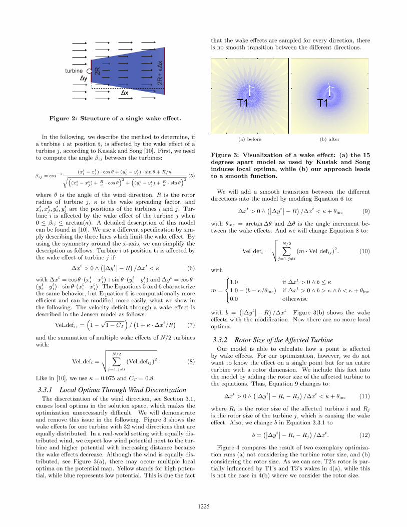
Figure 2: Structure of a single wake effect.

In the following, we describe the method to determine, ifa turbine i at position ti is affected by the wake effect of aturbine j, according to Kusiak and Song [10]. First, we needto compute the angle βij between the turbines:

βij = cos−1 (xti − xtj) · cos θ + (yti − ytj) · sin θ + R/κ√(

(xti − xtj) +Rκ · cos θ

)2+((yti − ytj) +

Rκ · sin θ

)2(5)

where θ is the angle of the wind direction, R is the rotorradius of turbine j, κ is the wake spreading factor, andxti, x

tj , y

ti , y

tj are the positions of the turbines i and j. Tur-

bine i is affected by the wake effect of the turbine j when0 ≤ βij ≤ arctan(κ). A detailed description of this modelcan be found in [10]. We use a different specification by sim-ply describing the three lines which limit the wake effect. Byusing the symmetry around the x-axis, we can simplify thedescription as follows. Turbine i at position ti is affected bythe wake effect of turbine j if:

∆xt > 0 ∧(∣∣∆yt∣∣−R) /∆xt < κ (6)

with ∆xt = cos θ ·(xti−xtj)+sin θ ·(yti−ytj) and ∆yt = cos θ ·(yti−ytj)−sin θ·(xti−xtj). The Equations 5 and 6 characterizethe same behavior, but Equation 6 is computationally moreefficient and can be modified more easily, what we show inthe following. The velocity deficit through a wake effect isdescribed in the Jensen model as follows:

Vel defij =(

1−√

1− CT)/(1 + κ ·∆xt/R

)(7)

and the summation of multiple wake effects of N/2 turbineswith:

Vel defi =

√√√√ N/2∑j=1,j 6=i

(Vel defij)2. (8)

Like in [10], we use κ = 0.075 and CT = 0.8.

3.3.1 Local Optima Through Wind DiscretizationThe discretization of the wind direction, see Section 3.1,

causes local optima in the solution space, which makes theoptimization unnecessarily difficult. We will demonstrateand remove this issue in the following. Figure 3 shows thewake effects for one turbine with 32 wind directions that areequally distributed. In a real-world setting with equally dis-tributed wind, we expect low wind potential next to the tur-bine and higher potential with increasing distance becausethe wake effects decrease. Although the wind is equally dis-tributed, see Figure 3(a), there may occur multiple localoptima on the potential map. Yellow stands for high poten-tial, while blue represents low potential. This is due the fact

that the wake effects are sampled for every direction, thereis no smooth transition between the different directions.

(a) before (b) after

Figure 3: Visualization of a wake effect: (a) the 15degrees apart model as used by Kusiak and Songinduces local optima, while (b) our approach leadsto a smooth function.

We will add a smooth transition between the differentdirections into the model by modifing Equation 6 to:

∆xt > 0 ∧(∣∣∆yt∣∣−R) /∆xt < κ+ θinc (9)

with θinc = arctan ∆θ and ∆θ is the angle increment be-tween the wake effects. And we will change Equation 8 to:

Vel defi =

√√√√ N/2∑j=1,j 6=i

(m ·Vel defij)2. (10)

with

m =

1.0 if ∆xt > 0 ∧ b ≤ κ1.0− (b− κ/θinc) if ∆xt > 0 ∧ b > κ ∧ b < κ+ θinc

0.0 otherwise

with b =(∣∣∆yt∣∣−R) /∆xt. Figure 3(b) shows the wake

effects with the modification. Now there are no more localoptima.

3.3.2 Rotor Size of the Affected TurbineOur model is able to calculate how a point is affected

by wake effects. For our optimization, however, we do notwant to know the effect on a single point but for an entireturbine with a rotor dimension. We include this fact intothe model by adding the rotor size of the affected turbine tothe equations. Thus, Equation 9 changes to:

∆xt > 0 ∧(∣∣∆yt∣∣−Ri −Rj) /∆xt < κ+ θinc (11)

where Ri is the rotor size of the affected turbine i and Rjis the rotor size of the turbine j, which is causing the wakeeffect. Also, we change b in Equation 3.3.1 to

b =(∣∣∆yt∣∣−Ri −Rj) /∆xt. (12)

Figure 4 compares the result of two exemplary optimiza-tion runs (a) not considering the turbine rotor size, and (b)considering the rotor size. As we can see, T2’s rotor is par-tially influenced by T1’s and T3’s wakes in 4(a), while thisis not the case in 4(b) where we consider the rotor size.

1225

(a) Rotor size not considered (b) Rotor size considered

Figure 4: Two sectors of a larger map (a) withoutand (b) with consideration of the affected turbines’rotor size.

4. GEOGRAPHICAL DATABesides a detailed wind model, we consider data from

OpenStreetMap [6] for a realistic geo-planning scenario. Thegeo-information adds constraints to our wind turbine place-ment optimization problem. In this section, we introduceOpenStreetMap and define three scenarios for the experi-ments.

4.1 OpenStreetMapOpenStreetMap is a community-driven project, which was

started in 2004 with the objective to create a license freeworld map. It contains geographical like positions of streetsand buildings. Neis et al. [14] come to the conclusion that“[...] at least in countries, in which the OSM project is welldeveloped, the data is becoming comparable in quality toother geodata from commercial providers [...]”. The datais provided in easily processable XML files containing thegeo-information. The overall amount of data is more than400 GByte. For Germany 3.6 GByte geodata are available.In our simulation model, we dynamically load the relevantdata for the corresponding sector and use the information todefine constrained areas on the target. We model that theminimum distance between a turbine i and a street shouldbe 1.5 · hi and 500 m to a building which is a good practice.

On the map plots in the remainder of this paper, yellowlines stands for streets, grey areas illustrate buildings andthe constrainted areas around streets and buildings are vi-sualized in red.

4.2 ScenariosIn this section, we introduce our scenarios to test the op-

timization algorithms. We focus on onshore wind farms. InLower Saxony most wind farms consist of fewer than 30 tur-bines [16], and we define scenarios with this in mind. Evenat this scale, a wind farm consisting of 20 Enercon E-101wind turbines with 3000 kW and 60% of full load hours pro-duces about 315 GWh/a. An output increase by 1% willincrease the value of the produced energy on the basis of aprice of 0.10 EUR/kWh by 315 000 EUR per year.

In the scenarios we define multiple constraints: (1) theOpenStreetMap data results in areas that are unavailablefor the placement of turbines, and (2) we require like Man-well [12] a minimum safety distance depending on the rotorsize r between every turbine i and j of 8 ·max(ri, rj).

(a) Scenario 2 (b) Scenario 3

Figure 5: Illustration of benchmark Scenarios 2and 3.

Scenario 1. In Scenario 1, the task is to place 25 turbineson an empty map of size msize = (3.0, 3.0) leading to an areaof 9 km2. The wind distribution is very similar to Figure 1.In addition, the potential in the right upper corner is slightlyhigher than on the rest of the map. A turbine will producenearly 700 kW in mean per year at this position if it is notinfluenced by wake effects.

Scenario 2. In the upper right corner of Scenario 2 in Fig-ure 5(a) Leerhafe, a part of the city Wittmund in LowerSaxony, can be seen. The scenario has the coordinates indecimal degrees 53.5015◦−53.5317◦, 7.7346◦−7.7836◦, withsize msize = (3.3, 3.3) leading to an area of 10.9 km2. It con-tains 250 buildings and 64 streets consisting of 489 parts.All these elements lead to constraints. As the scenario isnext to the position of the wind rose in Figure 1, the winddistribution is very similar to it.

Scenario 3. Scenario 3 on Figure 5(b) has many con-strained areas. It lies at the position 53.4023◦ −53.4433◦, 8.0743◦−8.1412◦. It employs sizemsize = (4.5, 4.5)resulting in an area of 20.3 km2 and contains 185 buildingsand 229 streets consisting of 1493 parts. Its wind distribu-tion can be seen in Figure 1.

5. EVOLUTIONARY STRATEGIESThe turbine placement problem is a continuous black-

box optimization problem f : RN → R with constraintsg : RN → B, i.e., a candidate solution x ∈ RN encodes thegeo-positions of N/2 turbines that can be feasible (g(x) = 0)w. r. t. geo-constraints or not (g(x) = 1). In our implemen-tation, a fitness function evaluation f first invokes a run ofthe geo-constraints module, and in case of feasibility a runof the wake model module determines the total power of thewind park. As fitness function f to maximize, we use thesum of the power output E of every turbine:

f(x) =

N/2∑i=1

E(ti). (13)

where ti is defined as in Equation 1. For optimization, weemploy evolution strategies, as they are strong blackbox op-timization heuristics in continuous solution spaces. In thissection, we present the optimization variants we employ inthe experimental section, and describe how solutions areinitialized and how constraints are handled. We use six

1226

strategies that can be categorized into two groups. Onegroup is formed by the strategies that optimize the solutionvector x without any knowledge about which value repre-sents which turbine. For this category we use the state forthe art CMA-ES and an adaptive (1 + 1)-ES. In the othergroup the strategies modify individual turbines. These ap-proaches use the knowledge which values represents whichturbine and coordinate. For this category we use a replacingstrategy, a deterministic (1 + 1)-ES, an adaptive (1 + 1)-ESand a new self-adaptive approach.

5.1 Constraint HandlingInfeasible solutions from the geo-constraints get a low fit-

ness, i.e., if g(x) = 1, we assign f(x) = 0. This is a variantof death penalty that does not require a modification of theoptimization algorithm with a feasibility control loop whilegenerating offspring candidate solutions. This type of deathpenalty is similar the approach by Morales and Quezada [13].

5.2 InitializationThe initialization of the turbine locations can play an im-

portant part in the optimization. We experiment with chess-board and random initialization to create the initial solutionx0. Chessboard initialization places the turbines equidis-tantly on a grid also taking into account the geo-constraints.If there is an infeasible area, the final chess pattern will looklike a chessboard with missing fields. Random initializationplaces the turbines randomly on the map but only at validpositions taking into account the geo-constraints, if applica-ble.

5.3 Holistic ApproachesIn the following, we introduce the optimization approach

we employ in the following experiments. As stated before,our optimization approaches can be classified into holisticones that treat the turbine placement task as N -dimensionaloptimization problem, and turbine-oriented approaches thatuse evolutionary operators oriented to the coordinates ti ofspecific turbines that are randomly chosen.

5.3.1 Adaptive (1 + 1)N -ESThe first holistic optimization approach is a simple (1+1)-

ES [3] with Gaussian mutation

x′ = x + σ · N (0, 1) (14)

and Rechenberg’s step size control [3], which works as fol-lows. The (1 + 1)-ES runs for a number Gr of generations.During this period, step size σ is kept constant and the num-ber Gs of successful mutations is counted. From Gs, thesuccess probability can be estimated as Ps = Gs/Gr. Stepsize σ is increased according to σ′ = σ · τ , if Ps > 1/5,and decreased otherwise, with τ > 1. We use τ = 1.1, whichturned out to be the best choice in preliminary experiments.The (1 + 1)-ES accepts the new candidate solution x′, if itsfitness is better than or equal to the fitness of x, i.e., iff(x′) ≥ f(x). The ES terminates after G generations.

5.3.2 CMA-ESUsing a CMA-ES [7] for optimizing wind turbines on an

empty map with various kinds of border shapes was alreadyconducted by Wagner et al. [18]. Their experiments showedthat the optimization results of the CMA-ES outperformedthe optimization module of the industry tool OpenWind [1].

The CMA-ES starts with an initial solution x0. The initialstandard deviation σ0 is set to σ0 = 10.0 corresponding to10 m. A small standard deviation makes constraint viola-tions less likely and prevents the CMA-ES to some extentfrom problems with infeasible mutations x′ while adjustingits covariance matrix C.

5.4 Turbine-oriented ApproachesThe mutation operators of turbine-oriented approaches

concentrate on the locations ti of subsets of turbines i ∈ T ,in particular they concentrate on only one turbine for eachmutation operator execution.

5.4.1 Adaptive (1 + 1)1-ESA special case of our turbine-oriented approaches is the

adaptive (1 + 1)1-ES that randomly selects one turbine i atlocation ti from the set of turbines {1, . . . , N/2}. From thisturbine, only one coordinate (xi or yi) is randomly selectedand subject to Gaussian mutation, see Equation 14. Like incase of the holistic adaptive (1 + 1)N -ES, Rechenberg’s stepsize control is employed.

5.4.2 ReplacingThe replacing optimization is a simple optimization ap-

proach. In every step, the algorithms removes randomlyone chosen turbine i at the position ti from the solution xand replaces the turbine i at a randomly chosen new posi-tion t′i to create a new solution x′. If the fitness functionvalue f(x′) is greater than f(x) the new solution is pickedas basis for the next step. So it is a very basic (1 + 1)-ESbut without any step size control.

5.4.3 Deterministic (1 + 1)t-ESLuckehe et al. [11] proposed a turbine-oriented determin-

istic (1 + 1)-ES to place and optimize iteratively turbineson a map with constraints. We use the optimization part ofthis approach and combine it with the initial solutions x0.In this approach, the (1 + 1)t-ES picks in every generationone turbine i with the position ti, and mutates it by movingi to a new position t′i. It applies:

t′i = ti + σ(g) ·msize · N (0, 1) (15)

with the step size:

σ(g) = 1.0−((

1.0− 1

G

)· gG

)(16)

where g is the actual number of generation and G the totalnumber of generations. After the mutation, the strategyevaluates the new solution and selects the solution with thehighest fitness function value.

5.4.4 Self-Adaptive (1 + λ)-ESWe want to improve the results by using a self-adaptive

(1 + λ)-ES. A self-adaptive step size σ ∈ [0, 1] should makeit possible to react more flexibly to the scenarios. New posi-tions are created like in Equation 15. We also want to extendthe options for the strategy, and we do this as follows. First,we add the capability to move multiple turbines at the sametime and not consecutively. How many turbines n shall bemoved at the same time is controlled self-adaptively. Thesecond new option for the strategy is to remove one turbineti from solution x and replace it at a new position t′i. The

1227

probability p ∈ [0, 1] that controls how often the strategymove or replace a turbine is also operated self-adaptively.

As step size σ and probability p are bound constrained,we employ the operator by Back and Schutz [2] for intervalconstrained self-adaptation:

σ′ =

(1 +

1− pp· eτ ·N (0,1)

)−1

. (17)

The parameter τ controls the magnitude of mutations. Wechoose the setting τ = 0.22 like proposed in [2]. The numbern of turbines to change in one step will be unchanged n′ = nwith the probability 2/3 and increased or decreased by 1with probability 1/6 with constraint n ≥ 1. In initial tests,a population size of 50 showed a good performance.

6. EXPERIMENTAL RESULTSIn this section, we experimentally analyze the optimiza-

tion variants introduced in the previous section on the threescenarios presented in Section 4.2.

6.1 Comparison of Evolutionary AlgorithmsTable 1 shows the results of the two initialization vari-

ants combined with the six introduced optimization algo-rithms on benchmark Scenario 1, which does not have geo-constraints. The row Init. shows the fitness at initialization.The figures show the mean fitness with corresponding stan-dard deviation and the best fitness achieved in 25 runs. Boldvalues show the best results achieved for Scenario 1, in which25 turbines have to be placed (N = 50).

Init. Chess RandomAlgo. Mean ± Std Max Mean ± Std MaxInit. 14679.9± 0.0 14679.9 14136.4±207.2 14573.6

(1+1)N 15169.1± 60.8 15281.6 14892.5±126.6 15083.3CMA 15356.5± 48.6 15418.9 15359.5±110.9 15449.6(1+1)1 15408.8± 22.2 15446.6 15461.4± 32.6 15510.6Rep. 15438.2± 25.1 15482.8 15443.8± 25.1 15505.5(1+1)t 15532.1±10.2 15552.0 15527.5±13.4 15551.0(1+λ) 15525.6± 17.3 15557.4 15524.6± 18.9 15556.4

Table 1: Experimental results of Scenario 1. Se-lected corresponding statistical test can be found inTable 4.

We can observe that all optimization heuristics achievea significant improvement in comparison to the initial so-lutions. The (1 + 1)t-ES achieves the best results in av-erage with a small standard deviation. The self-adaptive(1 + λ)-ES achieves the second best mean result, but at thesame time the best maximum of all strategies. The class ofholistic optimizers is outperformed by all turbine-orientedmethods, which is probably due to the fact that it treatsthe whole optimization problem in a holistic fashion, i.e.,all N variables at once, although strong dependencies existbetween the turbines. The (1 + 1)N -ES achieves the worstresults of all strategies and is outperformed by the CMA-ES,which has much stronger capabilities in adapting its Gaus-sian mutations. The replace strategy achieves higher windpotentials than the (1 + 1)1-ES in the chessboard initializa-tion case, and vice versa in the random intialization case.Both strategies are less specialized than the deterministic(1+1)t-ES and the self-adaptive turbine-oriented (1+λ)-ESand perform worse, but still clearly outperform the holisticvariants in mean and in the maximum achieved values. The

statistical significance of the most important observationsare confirmed with a Wilcoxon signed rank-sum test [9], seeTable 4.

Init. Chess RandomAlgo. Mean ± Std Max Mean ± Std MaxInit. 10944.2± 0.0 10944.2 10626.5±145.2 10875.3

(1+1)N 11221.3± 33.0 11287.3 11084.6±126.6 11280.2CMA 11359.7± 12.5 11386.6 11348.4± 89.8 11475.2(1+1)1 11399.3± 17.5 11444.5 11437.8± 47.8 11502.5Rep. 11484.0± 9.7 11505.0 11480.8± 12.1 11506.5(1+1)t 11524.1± 8.4 11538.2 11524.6± 6.6 11535.6(1+λ) 11516.5± 11.7 11537.2 11519.9± 9.7 11536.6

Table 2: Experimental results of Scenario 2.

Table 2 shows the experimental comparison of all evolu-tionary approaches on benchmark Scenario 2. This bench-mark problem is an N = 36-dimensional problem with 18turbines. We observe a similar behavior of the algorithms incomparison to Scenario 1. Again, the deterministic (1 + 1)t-ES and the self-adaptive (1 + λ)-ES outperform the otherapproaches. Further, we can observe that the replace strat-egy is better than the (1 + 1)1-ES for both initializationschemes, which is probably due to the highly constrainedsolution space.

Init. Chess RandomAlgo. Mean ± Std Max Mean ± Std MaxInit. 10537.7± 0.0 10537.7 10491.3±200.9 10815.4

(1+1)N 10675.3± 32.7 10774.6 10814.4±144.4 11098.4CMA 10831.0± 29.9 10859.1 11008.2±105.4 11187.8(1+1)1 10889.7± 51.5 11083.8 11083.6± 88.2 11234.1Rep. 11261.5± 9.9 11286.9 11261.8± 11.9 11280.5(1+1)t 11288.9± 8.0 11301.6 11286.0± 6.9 11300.7(1+λ) 11286.5± 9.8 11302.7 11283.8± 9.1 11295.8

Table 3: Experimental results of Scenario 3.

Last, we show the experimental results on Scenario 3 inTable 3. This problem employs the most constraints with17 turbines resulting in an N = 34-dimensional problem.Again, (1 + 1)t-ES and (1 + λ)-ES perform best, i.e., withchessboard initialization, the (1 + 1)t-ES achieves the bestmean result, but the (1 + λ)-ES reaches the highest fitness.With random initialization, the (1+1)t-ES achieves the bestmean and best overall fitness. Although the mean resultsare better, the (1 + 1)t-ES does not perform significantlydifferent than the (1 + λ)-ES, see the Wilcoxon test in Ta-ble 4. Further, we can observe that the quality of the replacestrategy is close to the two best turbine-oriented optimizers,probably because of the same argument like in Scenario 2,i.e., because of the highly constrained solution space.

CMA (1 + 1)t (1 + λ)

CMA +/+ /+ +/+ /+

(1 + 1)t +/+ /+ −/+ /−(1 + λ) +/+ /+ −/− /−

Table 4: Statistical significance of comparison be-tween selected experiments of Tables 1 to 3.

Table 4 shows an analysis of the statistical significanceof selected experiments of Tables 1 to 3 employing theWilcoxon signed rank-sum test. The runs of the CMA-ES,

1228

the (1 + 1)t-ES and the (1 + λ)-ES are compared to eachother on the three scenarios, corresponding to order of sce-narios. If the p-value is lower than 0.05, the difference of theruns is statistically significant with a significance level of 5%,indicated by ’+’, otherwise indicated by ’-’. The upper righttriangle of the table shows the results for chessboard initial-ization, while the lower left part shows the correspondingresults for random initialization.

In general, when comparing chessboard and random ini-tialization, random tends to result in higher standard de-viations. This is probably because of the varying startingconditions. Interestingly, there is no significant differencebetween chessboard and random initialization for the bestoptimization strategies (1 + 1)t-ES and (1 +λ)-ES resultingin a p-value greater than 0.05. For the (1 + 1)N -ES and the(1 + 1)1-ES, the initialization makes a significant difference.

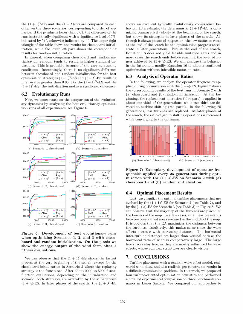
6.2 Evolutionary RunsNow, we concentrate on the comparison of the evolution-

ary dynamics by analyzing the best evolutionary optimiza-tion runs of all experiments, see Figure 6.

5000 15000 25000

14800

15200

15600

(1+ 1)N

CMA(1+ 1)t

(1+ 1)1

Rep.(1+ λ)

(a) Scenario 1, chessboard

5000 15000 2500014000

14400

14800

15200

15600

(1+ 1)N

CMA(1+ 1)t

(1+ 1)1

Rep.(1+ λ)

(b) Scenario 1, random

5000 15000 25000

11000

11200

11400

11600

(1+ 1)N

CMA(1+ 1)t

(1+ 1)1

Rep.(1+ λ)

(c) Scenario 2, chessboard

5000 15000 2500010400

10800

11200

11600

(1+ 1)N

CMA(1+ 1)t

(1+ 1)1

Rep.(1+ λ)

(d) Scenario 2, random

5000 15000 25000

10600

10800

11000

11200

11400

(1+ 1)N

CMA(1+ 1)t

(1+ 1)1

Rep.(1+ λ)

(e) Scenario 3, chessboard

5000 15000 25000

10200

10600

11000

11400

(1+ 1)N

CMA(1+ 1)t

(1+ 1)1

Rep.(1+ λ)

(f) Scenario 3, random

Figure 6: Development of best evolutionary runswhen optimizing Scenarios 1, 2, and 3 with chess-board and random initialization. On the y-axis weshow the energy output of the wind farm after xfitness evaluations.

We can observe that the (1 + 1)1-ES shows the fastestprocess at the very beginning of the search, except for thechessboard initialization in Scenario 3 where the replacingstrategy is the fastest one. After about 2000 to 5000 fitnessfunction evaluations, depending on the initialization andscenario, both strategies are overtaken by the self-adaptive(1 + λ)-ES. In later phases of the search, the (1 + λ)-ES

shows an excellent typically evolutionary convergence be-havior. Interestingly, the deterministic (1 + 1)t-ES is opti-mizing comparatively slowly at the beginning of the search,but shows its strengths in later phases of the search. Al-though it shows phases of stagnation, the low mutation ratesat the end of the search let the optimization progress accel-erate in later generations. But at the end of the search,Equation 16 does not yield feasible mutation rates and inmost cases the search ends before reaching the level of fit-ness achieved by (1 + λ)-ES. We will analyze this behaviorin the future and modify Equation 16 to allow a continuedoptimization without infeasible mutation rates.

6.3 Analysis of Operator RatiosIn the following, we analyze the operator frequencies ap-

plied during optimization with the (1+λ)-ES. Figure 7 showsthe corresponding results of the best runs in Scenario 2 with(a) chessboard and (b) random initialization. At the be-ginning, the replacement operation (blue part) is applied inabout one third of the generations, while two third are de-voted to turbine shifting (red parts). In the following 25generations, less turbines are replaced. At later phases ofthe search, the ratio of group shifting operations is increasedwhile converging to the optimum.

5x25 10x25 15x25 20x250

5

10

15

20

25

(a) Scenario 2 (chessboard)

5x25 10x25 15x25 20x250

5

10

15

20

25

(b) Scenario 2 (random)

Figure 7: Exemplary development of operator fre-quencies applied every 25 generations during opti-mization with the (1 + λ)-ES on Scenario 2 with (a)chessboard and (b) random initialization.

6.4 Optimal Placement ResultsLast, we visualize the optimal turbine placements that are

evolved by the (1 + 1)t-ES for Scenario 2 (see Table 2), andby the (1+λ)-ES for Scenario 3 (see Table 3) in Figure 8. Wecan observe that the majority of the turbines are placed atthe borders of the map. In a few cases, small feasible islandsbetween constrained areas are used in the middle of the map.It is obvious that the EA maximizes the distances betweenthe turbines. Intuitively, this makes sense since the wakeeffects decrease with increasing distance. The horizontalinter-turbine distances are larger than vertical ones as thehorizontal ratio of wind is comparatively large. The largefree spaces stay free, as they are mostly influenced by wakeeffects, whose complex structures are clearly visible.

7. CONCLUSIONSTurbine placement with a realistic wake effect model, real-

world wind data, and also realistic geo-constraints results ina difficult optimization problem. In this work, we proposedfour turbine-oriented optimization heuristics and performeda detailed experimental comparison on three benchmark sce-narios in Lower Saxony. We compared our approaches to

1229

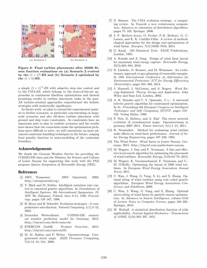
(a) Scenario 2 (b) Scenario 3

Figure 8: Final turbine placements after 25000 fit-ness function evaluations on (a) Scenario 2 evolvedby the (1 + 1)t-ES and (b) Scenario 3 optimized bythe (1 + λ)-ES.

a simple (1 + 1)N -ES with adaptive step size control andto the CMA-ES, which belongs to the state-of-the-art ap-proaches in continuous blackbox optimization and showedpromising results in turbine placement tasks in the past.All turbine-oriented approaches outperformed the holisticstrategies with statistically significance.

As future work, we plan to extend the experimental analy-sis to further scenarios, in particular concentrating on large-scale scenarios and also off-shore turbine placement withground and ship route constraints. As constraints have animportant part to play in realistic scenarios and the resultshave shown that the constraints make the optimization prob-lems more difficult to solve, we will concentrate on more ad-vanced constraint handling techniques in the future, rangingfrom penalty function to meta-modeling of the constraintboundary.

AcknowledgementsWe thank the German Weather Service for providing theCOSMO-DE data and the Ministry for Science and Cultureof Lower Saxony for supporting this work with the PhDprogram System Integration of Renewable Energy (SEE).

References[1] AWS Truepower. AWS Openwind, 2008.

http://awsopenwind.org/.

[2] T. Back and M. Schutz. Intelligent mutation rate con-trol in canonical genetic algorithms. In Foundations ofIntelligent Systems, 9th International Symposium, IS-MIS ’96, Zakopane, Poland, June 9-13, 1996, Proceed-ings, pages 158–167, 1996.

[3] H. Beyer and H. Schwefel. Evolution strategies - A com-prehensive introduction. Natural Computing, 1(1):3–52,2002.

[4] Deutscher Wetterdienst. COSMO-DE: numeri-cal weather prediction model for Germany, 2012.http://tinyurl.com/dwd-cosmo-de.

[5] ENERCON GmbH. Product Overview, 2015.http://tinyurl.com/enercon101.

[6] M. M. Haklay and P. Weber. Openstreetmap: User-generated street maps. IEEE Pervasive Computing,7(4):12–18, Oct. 2008.

[7] N. Hansen. The CMA evolution strategy: a compar-ing review. In Towards a new evolutionary computa-tion. Advances in estimation of distribution algorithms,pages 75–102. Springer, 2006.

[8] J. F. Herbert-Acero, O. Probst, P.-E. Rethore, G. C.Larsen, and K. K. Castillo-Villar. A review of method-ological approaches for the design and optimization ofwind farms. Energies, 7(11):6930–7016, 2014.

[9] G. Kanji. 100 Statistical Tests. SAGE Publications,London, 1993.

[10] A. Kusiak and Z. Song. Design of wind farm layoutfor maximum wind energy capture. Renewable Energy,35(3):685–694, 2010.

[11] D. Luckehe, O. Kramer, and M. Weisensee. An evolu-tionary approach to geo-planning of renewable energies.In 28th International Conference on Informatics forEnvironmental Protection: ICT for Energy Effieciency(EnviroInfo), pages 501–508, 2014.

[12] J. Manwell, J. McGowan, and A. Rogers. Wind En-ergy Explained: Theory, Design and Application. JohnWiley and Sons Ltd, London, 2002.

[13] A. K. Morales and C. V. Quezada. C.v.: A universaleclectic genetic algorithm for constrained optimization.In In: Proceedings 6th European Congress on IntelligentTechniques and Soft Computing (EUFIT, pages 518–522. Verlag Mainz, 1998.

[14] P. Neis, D. Zielstra, and A. Zipf. The street networkevolution of crowdsourced maps: Openstreetmap ingermany 2007–2011. Future Internet, 4(1):1–21, 2011.

[15] H. Neustadter. Method for evaluating wind turbinewake effects on wind farm performance. Journal of So-lar Energy Engineering, pages 107–240, 1985.

[16] The Wind Power. Wind farms in Lower Saxony, Ger-many, 2015. http://tinyurl.com/parks-lower-saxony.

[17] M. Wagner, J. Day, and F. Neumann. A fast and effec-tive local search algorithm for optimizing the placementof wind turbines. Renewable Energy, 51(0):64–70, 2013.

[18] M. Wagner, K. Veeramachaneni, F. Neumann, and U.-M. O’Reilly. Optimizing the layout of 1000 wind tur-bines. In European Wind Energy Association AnnualEvent, 2011.

[19] C. Wan, J. Wang, G. Yang, X. Li, and X. Zhang. Op-timal siting of wind turbines using real coded geneticalgorithms. European Wind Energy Association Con-ference and Exhibition, 2009.

[20] C. Wan, J. Wang, G. Yang, and X. Zhang. Optimalmicro-siting of wind farms by particle swarm optimiza-tion. In Advances in Swarm Intelligence, volume 6145of Lecture Notes in Computer Science, pages 198–205.Springer, 2010.

[21] W. Weibull. A statistical distribution function of wideapplicability. Journal Applied Mechanics - Transactionsof ASME, 3(18):293–297, 1951.

1230