Bulletin Number 95-1

ECONOMIC DEVELOPMENT CENTER

ON ENDOGENOUS GROWTH: THE IMPLICATIONS 01ENVIRONMENTAL EXTERNALITIES

Elamin H. Elbasha and Terry Ro<

ECONOMIC DEVELOPMENT CENTER

Department of Economics, MinneapolisDepartment of Agricultural and Applied Economics, St. Paul

UNIVERSITY OF MINNESOTA

February 19S

On Endogenous Growth: The Implications of Environmental Externalities

Elamin H. Elbasha and Terry L. Roe*

January 27, 1995

Abstract

This paper uses an endogenous growth model to examine the interaction between trade, economicgrowth, and the environment. We find that whether trade enhances or retards growth depends on therelation between factor intensities of exportable, importable, and R&D and the relative abundanceof the factor R&D uses more intensively. Depending on the intertemporal elasticity of substitution,the long-run rate of economic growth changes with environmental externalities. Concerns about theenvironment can explain a significant part of cross-country difference in growth rates. For theempirically reported range of the elasticity of intertemporal substitution, countries which care moreabout the environment grow faster. The effects of trade on the environment and welfare depend onthe elasticities of supply for the two traded goods, the terms of trade effect on growth, and pollutionintensities. The decentralized and Pareto optimal growth rates are, in general, different. The marketgrowth rate is bigger than the optimal rate the larger the degree of monopoly power in the innovationsector and the stronger the effects of environmental externalities. The policy implications of thisdivergence are discussed. We also consider numerical exercises to broaden the insights from theanalytical results and allow for incorporating pollution abatement (Journal ofEconomic LiteratureClassification Numbers: F11, 031, 041, Q20).

Key Words

Endogenous growth, environment, innovation, trade.

*Graduate Student and Professor, respectively, Department of Agricultural and Applied Economics, Universityof Minnesota. Funding for this research was provided by USAID/EPAT/MUCIA.

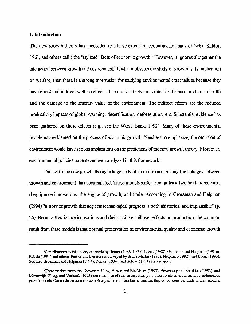
I. Introduction

The new growth theory has succeeded to a large extent in accounting for many of (what Kaldor,

1961, and others call ) the "stylized" facts of economic growth.' However, it ignores altogether the

interaction between growth and environment. 2 If what motivates the study of growth is its implication

on welfare, then there is a strong motivation for studying environmental externalities because they

have direct and indirect welfare effects. The direct effects are related to the harm on human health

and the damage to the amenity value of the environment. The indirect effects are the reduced

productivity impacts of global warming, desertification, deforestation, etc. Substantial evidence has

been gathered on these effects (e.g., see the World Bank, 1992). Many of these environmental

problems are blamed on the process of economic growth. Needless to emphasize, the omission of

environment would have serious implications on the predictions of the new growth theory. Moreover,

environmental policies have never been analyzed in this framework.

Parallel to the new growth theory, a large body of literature on modeling the linkages between

growth and environment has accumulated. These models suffer from at least two limitations. First,

they ignore innovations, the engine of growth, and trade. According to Grossman and Helpman

(1994) "a story of growth that neglects technological progress is both ahistorical and implausible" (p.

26). Because they ignore innovations and their positive spillover effects on production, the common

result from these models is that optimal preservation of environmental quality and economic growth

'Contributions to this theory are made by Romer (1986, 1990), Lucas (1988), Grossman and Helpman (1991 a),Rebelo (1991) and others. Part of this literature is surveyed by Sala-i-Martin (1990), Helpman (1992), and Lucas (1993).See also Grossman and Helpman (1994), Romer (1994), and Solow (1994) for a review.

2There are few exceptions, however. Hung, Victor, and Blackburn (1993), Bovenberg and Smulders (1993), andMarrewijk, Ploeg, and Verbeek (1993) are examples of studies that attempt to incorporate environment into endogenousgrowth models. Our model structure is completely different from theirs. Besides they do not consider trade in their models.

1

are competitive objectives. This result is in contradiction with what many economists believe (e.g.,

see World Bank, 1992). Second, they tend to place emphasis on analyzing optimal growth only (even

though economies do not behave optimally) rather than also considering a market driven dynamic

equilibrium.3 Studies that use market analysis concentrate on the cost of environmental policy and

ignore externalities which are at the heart of environmental economics.4

These gaps need to be filled. We need to have a better understanding of the linkages between

innovations, trade, economic growth, and environmental quality. In other words, we are in need of

a framework that integrates the theory of endogenous economic growth, the theory of international

trade, and environmental economics. It should enable us to answer questions like the following. What

are the implications of introducing environmental considerations in a standard endogenous growth

model? Does environment slow or accelerate growth? What are the repercussions of trade? Dose

trade liberalization increases the long-run rate of economic growth? Dose it improve or worsen the

quality of the environment? Is trade welfare improving as it is oftentimes true in the absence of

environmental externalities? Faced with environmental externalities, how can an economy optimally

innovate and grow over time? Is a competitive equilibrium Pareto optimal and, if not, what are the

policy implications? Are there first-best policies? If first best policies are not available, would there

be second-best policies?

This paper attempts to model the link between innovations, trade, growth, and environmental

'Examples from this category are: Keeler, Spence, and Zechkauser (1971); D'Arge and Kogiku (1972); Gruuver(1976); Krautkraemer (1985); and Nordhaus (1991a, 1991b, 1992, 1993). An exception is Tahvonen and Kuuluvainen(1993) who analyze competitive equilibrium. In their model, however, technological change and trade issues are ignored.

4Examples are: Jorgenson and Wilcoxen (1990a, 1990b, 1993a, 1993b), Blitzer et al. (1993), Manne and Richels(1990), Burniaux et al. (1992). There is also a growing literature on the empirical aspects of growth and environment nexus.(See for example Grossman and Krueger (1993, 1994), Skafik and Bandyopadhyay, 1992). One major limitation of this workis that the estimated relationship is not derivable from a theoretical model.

2

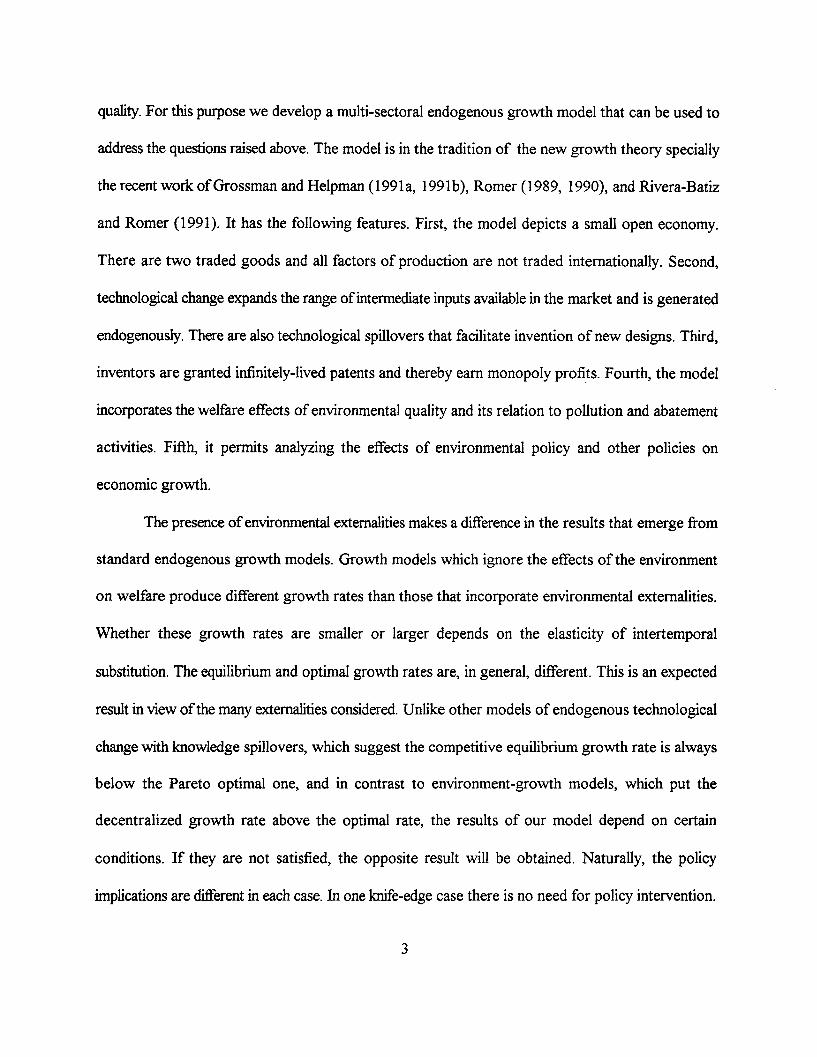
quality. For this purpose we develop a multi-sectoral endogenous growth model that can be used to

address the questions raised above. The model is in the tradition of the new growth theory specially

the recent work of Grossman and Helpman (1991a, 199 1b), Romer (1989, 1990), and Rivera-Batiz

and Romer (1991). It has the following features. First, the model depicts a small open economy.

There are two traded goods and all factors of production are not traded internationally. Second,

technological change expands the range of intermediate inputs available in the market and is generated

endogenously. There are also technological spillovers that facilitate invention of new designs. Third,

inventors are granted infinitely-lived patents and thereby earn monopoly profits. Fourth, the model

incorporates the welfare effects of environmental quality and its relation to pollution and abatement

activities. Fifth, it permits analyzing the effects of environmental policy and other policies on

economic growth.

The presence of environmental externalities makes a difference in the results that emerge from

standard endogenous growth models. Growth models which ignore the effects of the environment

on welfare produce different growth rates than those that incorporate environmental externalities.

Whether these growth rates are smaller or larger depends on the elasticity of intertemporal

substitution. The equilibrium and optimal growth rates are, in general, different. This is an expected

result in view of the many externalities considered. Unlike other models of endogenous technological

change with knowledge spillovers, which suggest the competitive equilibrium growth rate is always

below the Pareto optimal one, and in contrast to environment-growth models, which put the

decentralized growth rate above the optimal rate, the results of our model depend on certain

conditions. If they are not satisfied, the opposite result will be obtained. Naturally, the policy

implications are different in each case. In one knife-edge case there is no need for policy intervention.

We explore several policies that could align the two growth paths. Whether trade enhances or

frustrates growth depends on the relation between factor intensities of the two final output sectors

and that of the research and development sector and the relative abundance of the factor that R&D

uses more intensively. The effects of trade on environment and welfare are ambiguous. They depend

on a number of conditions that will be shown.

The paper is organized as follows. The model is presented in Section II. The "competitive"

equilibrium and the determinants of sustained growth are derived in Section III. We also study the

effects of consumers' attitude toward the environment on growth. In Section IV, the solution to a

social planner's problem is discussed and compared to the market solution. We also derive the

conditions under which the two solutions are different. Section V focuses on how intervention can

secure optimal allocations of resources.

The model of Section II assumes firms cannot control pollution even if they wish to. Section

VI extends this model to incorporate the ability of firms to control pollution. In this model there is

an effluent charge on pollution emitted into the environment. Technological knowledge reduces the

cost of controlling pollution. Because of the difficulty of finding analytical solutions, we solve the

model numerically. In Section VII we summarize our results and provide concluding remarks.

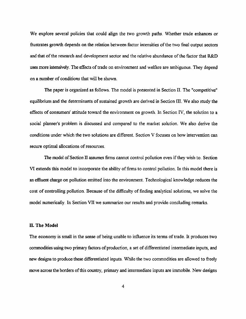
II. The Model

The economy is small in the sense of being unable to influence its terms of trade. It produces two

commodities using two primary factors of production, a set of differentiated intermediate inputs, and

new designs to produce these differentiated inputs. While the two commodities are allowed to freely

move across the borders of this country, primary and intermediate inputs are immobile. New designs

are assumed to be nontradable. We will also assume that exchange of knowledge is not possible.

Consumers. There are many identical infinitely-lived consumers who get utility from the two traded

goods and the environment. Momentary utility of a representative consumer is given by5

(C ' C l-. Q90 - 1{ (C :+CI-*)Q")1 -1-I, for 0 < o < 0 o 1-, =- 1 - a(1)4 log Cy + (1- 0) log C, + plog Q, for o = I

0 . 4 : 1, A O0 4 (1-oa)< 1, pl(-o) < 1,

where Ci is consumption of commodity i (i = Z, Y) and Q is a variable measuring the quality of the

environment and will be described in more details later. Throughout this paper all Greek letters and

A's are parameters. All other variables should be thought of as functions of time unless otherwise

noted. We drop the time symbol to simplify the exposition. Consumers are endowed with two primary

factors of production, capital (K) and labor (L) whose supply is fixed every period6.

Final output sectors. There are two sectors that produce final output. Each sector consists of a large

number of identical firms. At the beginning of each period they rent labor and capital from consumers,

and a set of differentiated inputs from the intermediate inputs sectors. Production functions of the two

traded goods are given by

Y=A K,'L £D, A >0, a = 1, >0, = 1,2,3 (2)L-1

5This utility function exhibits the following properties (i) the elasticity of the marginal rate of substitution betweenconsumption and environmental quality with respect to consumption, [alog (U6/U, )/ alog Cj, is equal to one; (ii) theelasticity of the marginal utility of consuming commodity i is constant; (iii) the elasticity of the marginal utility ofenvironmental quality is constant and equal to 1-(1-a); and (iv) it satisfies Inada conditions: lim U, = °, lim U, = 0,lim UQ = , and lim UQ = 0. This is the only functional form compatible with steady state. Ci-0 co

Q-o Q-6Elbasha (1995) analyzes the implications of environmental externalities in three classes of endogenous growth

models that allow factor accumulation. All these are, however, closed economy models.

5

z A.KP'L.PD A.0, . 1, > 0, i = 1. 2 3, (3)it-

where K, is capital used in producing commodity i, Li is labor used in the production of good i, and

Di (i = y, z) denotes an index of differentiated inputs and is determined according to7

D,= [fX )bdj], 0 < 6 < 1, (4)

where M(t) denotes the measure (number) of differentiated products available at time t and X(j) is

the amount of differentiated input j. The set of brands available at time t, {i: i e [0, M(t)]}, is assumed

to be continuous. We also assume that both commodities Y and Z have the same intensity in D (i.e.

a3 = 033). This, together with the constant returns to scale restrictions, imply c( + a2 = P1 + P2.

Intermediate inputs Sectors. Each brand j e [0, M(t)] of differentiated inputs is produced by a single

firm. Firms have to obtain a license to use the blueprints for producing a brand from the R&D sector

before production starts . Once the license is acquired a firm can produce as much quantity ofX(j)

it wishes according to the following Cobb-Douglas technology

X(j) = A, [Kx(j)] [L(j)]l", A > 0, 1 > I > 0, j [0,M], (5)

where Lx(j) and KX(j) denote labor and capital used to produce X(j), respectively. The above

specification restricts the technology to be the same in all intermediate inputs sectors.

R&D sector. Research and development are undertaken in this sector. Firms use labor, capital, and

a public good (knowledge capital) to produce new blueprints and thereby add to the set of available

7This is the famous Dixit and Stiglitz 's (1977) formulation of horizontal product differentiation. Ethier (1982)reinterpreted equation (5) as a production function instead of a utility function as in Dixit and Stiglitz (1977).

6

brands. So, product development in the R&D sector evolves according to

M = AK.L M, A. > 0, 1 > 8 > 0, (6)

where a dot over a variable stands for the time derivative of that variable, Km is capital, Lm is labor

used in R&D sector, and M, the measure of differentiated inputs, is assumed to be proportional to

knowledge capital. We choose units of measure appropriately such that the factor of proportionality

is one.

Environmental quality. To avoid adding another state variable to the system, we model the quality

of the environment as a flow variable. We offer two formulations. First, environmental quality is

determined by the following geometric index

Q = AE E, AQ > 0, y E < 0, (7)

where Ey and E, denote total emissions from sectors Y and Z, respectively. Emission levels are

assumed to be proportional to the respective aggregate quantities of Y and Z produced. One can

think of Y as denoting agriculture which contaminates the water system and Z as industry which

generates air pollution. The quality of the environment is, therefore, given by the inverse of the

geometric index of water and air pollution. In the second approach, we assume that use of

differentiated intermediate inputs generates pollution which impairs the ability of people to enjoy the

quality of the environment. We choose the following functional form to describe this

Q = [fX(t)(j)dj]-1, > 0. (7')

We assume agents are atomistic and take prices and the quality of the environment as given.

7

Market Structure. The markets for the two traded goods (Y and Z), labor, capital, and new designs

from the R&D sector are perfectly competitive. However, each producer of a differentiated input sells

its output in an imperfectly competitive market.

I. Equilibrium Analysis

We define equilibrium in the following way. An equilibrium is paths for prices and quantities such that

1. Consumers makes consumption and asset accumulation decisions treating prices, interest

rate, and environmental quality as exogenous functions of time.

2. Final output producers choose quantities of labor and capital taking output prices, prices

of primary and intermediate factors, and the measure of intermediate inputs as given.

3. Intermediate inputs producers maximize profits taking as given the price of labor and

capital, final output prices, the downward-sloping demand for their products, the number of

differentiated inputs, and the initial cost of obtaining a design.

4. Firms in the R&D sector choose labor and capital to create new designs taking as given the

price of new designs, prices of primary factors, and the stock of knowledge as given.

5. All markets clear.

We assume that all agents have perfect foresight so that at each moment of time the entire

path of prices is known. We will also assume that our small economy operates within its cone of

diversification ruling out specialization in the production ofZ and Y.

Profit maximization in the final good sectors requires equating unit costs to prices. That is8,

8Intermediate inputs producers cannot price discriminate between sectors because the price elasticities ofdemand are the same in the two sectors, see equation (12) below. The unit cost functions in equations (8) and (9) arederived as min wL L, + wk K+ pd Di s.t. (2) and Y = 1 for i =y, and s.t. (3) and Z= 1 for i= z. That in equation (10) is

8

Py, = Wk w (8)

PI P2 P3P = Wk WL Pd (9)PV (9)

a 8-1

Pd= If$Mpx(j)"-dj ] (10)

where wk denotes the price of capital, wL is price of labor, Pd is price of the index D, px(j) is price of

intermediate inputs j, and py and p, are prices of commodity Y and Z, respectively. Notice that in

deriving the unit cost functions we have chosen the constants of the production functions

appropriately.

Equilibrium in the R&D sector requires equating the price of a design to its unit cost. That

is,

e 1-8

P. W WL (11)A/M

where p. is the price of a new design and Am' = Am 0 (1-0)1'.

Applying Shephard's lemma to the unit cost function in equation (10), we can derive the

demand for Xk() as

1 6 1

x,j) = pO)-'D, [If p,(s)6-'ds] , i = y, z, j e [O,M]. (12)

Each firm in the intermediate goods sectors, acting monopolistically, maximizes profits taking into

obtained by minimizing f0Mp(i) X(i) di s.t. (4) and D = 1.

account the demand functions in equation (12). Profits are maximized by following the mark-up over

marginal cost pricing rule

P = W = WL v j E [O,M]. (13)b

Therefore, price, quantity, and hence the level of profits are the same for all firms operating in the

intermediate inputs sectors. Using this fact in equation (10) yields

6-1

P, = PM , (10')

where px denotes the common equilibrium price in the intermediate inputs sectors.

The cost functions in equations (8), (9), (10'), and (13) can be solved for input prices. The

solutions for the price of labor and capital are given by

In this equilibrium we will assume that world prices and the rate of innovation, M/M, are constant

over time. Hence, equations (14) and (15) imply

PL _*k _z 3(1-6) (16)

L = P.) p 1 M (14)

-wi 8g (16)(1

where g = /M. ThisM with equation (11), yields(15)

In this equilibrium we will assume that world prices and the rate of innovation, M/M, are constant

over time. Hence, equations (14) and (15) imply

10

P. [C(A- 8) - 81P1 . (17)

From the unit cost functions, using Shephard's lemma, we obtain the following input-output

coefficients:

P p P, , P= - PP

by = Lby =, , bb = n , b = 0P ,by =Wk Wk Wk Wk WL

(18)PZ XPa Py Pz

bz = p2 -P b = (1-l) P, bk- = (1-0)- , b = a" , b = p3WL WL WL Px Px

where by denotes per unit input i used in the production of good j, i = k, L, x and j = y, z, x, m.

Substituting these in the resource constraints, making use of the identity pxXM = pd(D + DO = c3pyY

+ 33pz Z, and rearranging gives

(ac+6al )p yY + (P+an+ P3pZ + ep.Mg = wkK (19)

[Ca,+(1- )a3] pyY + [P,+6(1-)P 13 PZ + (1-6) pM g = WLL. (20)

Since g, p, and py are constant, equations (19) and (20) suggest that both Y and Z grow at the same

rate of growth as that of wE and wk. That is,

- 2;- (1-g. (21)Y Z 6

Adding equations (19) and (20) and making use of some of the restrictions on the parameters yields

11

[1- a&(1 - )](pZ + pY) = wK + wL - p.Mg

Because firms are allowed to freely enter into and exit from R&D, in equilibrium, the price

of a new design is equivalent to the value of a firm in the intermediate inputs sectors. To maintain

asset market equilibrium, the rate of return from holding equities (i.e. dividends plus changes in the

value of the firms) should be equal to the rate of return on a one period loan. Thus, in equilibrium the

following no-arbitrage condition is satisfied

S + -= r, (23)Pm Pm

where x denotes the profit level of a firm in the intermediate inputs sectors, and r is the rate of

interest on loans. Using the fact that x/pm= (1-8)pxX/pm = (1-6)pdD/Mpm= (1-6)a 3(pyY +PzZ)/Mpm,

with equations (17) and (22), we can rewrite the above condition as

(1-), (wL + wK - pMg) a,(1-8)+ [ - l]g = r. (23')[1-a3(1-8)] Mp. 8

Utilizing equation (1), the consumer's indirect utility function is

[(EQ )/p Pzl"0 1'1-- 1V(E,pYpQ) = [(EQ)/p

(C Cz I-o _ 1Max s.t. pC + pzCz =

E,1-0Y

12

(22)

where E stands for expenditure. The solution to the consumer's problem is given by solving the

following dynamic problem

Max " V(E,pYp.,Q) e-t dt{E(t))

s.t. E + A(t) = ra(t) + wK + wLL

where a(t) denotes nonhuman wealth at time t. Application of the Maximum Principles results in the

following relation

o- - (- o)= r - p. (25)E Q

Due to the nature of the utility function, and because consumers have perfect information and rational

expectations (perfect foresight in this case), changes in the quality of the environment affect the path

of consumption over time. It is interesting to note that even though consumers take Q as given, its

evolution affects their behavior. Notice that if o = 1 (i.e. the utility is of the logarithmic form) or if

the utility is additively separable in Q, the second term in equation (25) will disappear and so the

consumption path will not be affected by Q.

We assume that our small country cannot lend or borrow from the outside world. Hence,

,trade is always in balance

E = pY + pz. (26)

Differentiating equation (26) with respect to time and making use of equation (21) gives

E _ (1- 8))-- =g. (27)

E

13

We can also combine equations (7) or (7') and (21) to obtain

- . (28)

if equation (7) applies or

Q _ (E - 1)- (28')Q

when (7') is the relevant equation. Substituting equations (27) and (28) into equation (25) and

rearranging yields

a 3(1-8)r = p + 1' a (29)

where T = o - p(1-o)(ey+E). If instead we use equation (28') we get r = p + T' a 3(1-6)g/6, where

Y' = o - p(1-o)(e-1)8/(1-6)Ea 3. Solving for wL/wk from equations (14) and (15) and combining

equations (11), (23'), and (29) and rearranging gives the growth rate of innovation in terms of the

parameters of the model, endowments, and exogenous variables

8 1AA .P'1 6 1 [(P)l-1K + L] - p

Pg P, (30)

1 + A + (7(F-1)

where A = a3(1-6)/[1-a 3(1-6)]. If equation (7') applies, we will have I' instead of T in the growth

formula. It should be noted that the integral in the consumer's utility function is always finite provided

c3(1I-)(1-)g/6 < p. The transversality condition associated with the consumer's problem ensures

the satisfaction of this inequality. The fact that we looked only for interior solution to the R&D sector

14

problem implicitly imposes a restriction on the growth formula in equation (30): growth has to be

strictly positive. We assume our parameters satisfy this and the condition required for boundedness

of the utility function. Both the numerator and denominator in equation (30) are taken to be positive.

In this model the effects of environmental externalities are captured by the parameters - g(Ey

+ e) if equation (7) applies or g(€-1)86/a 3(1-8) if equation (7') is the relevant equation. We adopt

the assumption that the effects of environmental externalities are mild relative to expenditure on

consumption i.e. 1 > - g(Ey + e) if equation (7) applies and 1 > gI(E-1)6/Ea 3(1-8) if we have equation

(7') instead. In other words, we assume consumers value consumption more than environmental

quality.

Claim. If consumers value consumption more than environmental quality, T > 0, and , 7'

is greater, equal to, or less than one as a is greater, equal to, or less than one; respectively.

Proof Rearrange the formulas for Y and T' the result is obvious.

The comparative static results of the growth rate are summarized by the following propositions.

Proposition 1. Growth is higher (i) the larger is the country's endowment of K andL, (ii) the

more productive is R&D (higher A'" ), (iii) the smaller the rate of time preference, (iv) the larger

the elasticity of intertemporal substitution (I/a), or (v) the smaller the elasticity of substitution (

lower 6) provided 7 s 19.

Proof The denominator in equation (30) is positive. Differentiating that equation with respect

to the relevant variable we get (i) ag/aK = A'm(py /pz) 1ey" ~'~P) /(denominator) > 0, ag/aL = A'm(py

/p ((x-diP) /(denominator) > 0; (ii) ag/9A'm = 1/(denominator) > 0; (iii) ag/ap = -1/(denominator) <

9According to Lerner (1934) price minus marginal cost divided by price measures the degree of market power. Inour case, this is given by 1 - 8. Therefore, an increase in the degree of market power (i.e. lower 6) increases growth.

15

0; (iv) ag/ao = [- g/(denominator)2 ]aW/ao. But aT/oa > 0. hence, ag/ao < 0; (v) dg/86 =

[denominator (numerator - A ) + a3(TY-1)/8 2]/(denominator)2, where 0 = (p, /p) 1-eoY(.1-1) K + (py

/p)-e/(•-p) L. But 8A/56 < 0 and (numerator - AQ) > 0. Hence, ag/a6 < 0.

Proposition 2. With the source of environmental externalities as described by equation (7),

environmental quality decays at a constant rate along the balanced growth path. If instead pollution

is governed by equation (7), environmental quality decays, stays constant, or improves at a constant

rate as e is less, equal to, or greater than one; respectively.

Proof. See equation (28) and (28').

II.1 The effects of environmental externalities on growth

Let the quality of the environment be given by equation (7). Then, taking environment into account

slows growth if the elasticity of intertemporal substitution (1/o) is greater than one. This can easily

be seen from the growth formula in equation (30). If agents ignore the effects of the environment (i.e.

t = 0), the denominator of equation (30) will be smaller and hence growth will be higher. This result

implies that countries in which consumers care more about the effects of environmental externalities

grow faster than those which don't. Moreover, growth is lower, the more profound are the effects

of the environment on consumer's utility (i.e. lower g), provided a < 1. If a > 1, the opposite result

will be obtained: growth varies positively with agents care about the effects of environment. It may

be interesting to note that if a = 1 (i.e. the case of a logarithmic utility) or if the utility function is

additively separable, the environment doesn't affect the growth rate under the competitive conditions

assumed. Changes in the elasticities of environmental quality with respect to pollution levels (ey and

e) have the opposite qualitative effects on growth compared to changes in Ct. We have proved the

following proposition.

16

Proposition 3. Care about the environment slows, doesn't affect, or promotes growth if and

only if the elasticity of intertemporal substitution (I/a) is greater, equal to, or less than one;

respectively. If the quality of the environment is given by equation (7), the above results hold only

if E < 1. When e > 1, we obtain the opposite qualitative result. If e = 1, environment does not affect

growth.

To get a feeling of the importance of incorporating environment in this endogenous growth

model follow this simple numerical exercise. Let a 3(1-6)/6 = 1, A'm = 0.075, py = pz = L = K = 1, 6

= 1/3, 65 + eZ = -1, 0 = 1.8, and p = 0.025. Choose g = 0 and use equation (30) to compute g as

2.17%. If p = 0.9, then g = 3.16%. Therefore, about 1% difference in growth rates across countries

can be explained by concern about the environment. Needless to emphasize, we could have chosen

the parameters in a way that would magnify this disparity.

111.2 The terms of trade effects

Assume that commodity Y is exported and Z is imported. Normalize the initial terms of trade to one,

and to neutralize the effects of endowments, suppose K = L. Then we have the following proposition.

Proposition 4. Let R&D be capital intensive (i.e. 0> 1/2). Then an improvement in the terms

of trade (i.e. higher p, /p) enhances (retards) growth if Y is less (more) capital intensive than Z.

Proof. If we differentiate equation (30) and use the above restrictions we arrive at:

sign[dg/a(py/p)] = sign[(a 1 - P3 ) (0 - 1/2)]. The proof follows immediately.

The intuition behind this result is simple. Stopler-Samuelson theorem suggests a fall in wk and

a rise in wL as a result of the rise in py/pa if Y is less capital intensive than Z. Hence the demand for

capital in R&D (which is capital intensive) increases and so does the growth rate. The above result

suggests that improvements in the terms of trade boosts growth only if whatever factor intensity R&D

17

has, exportables have less of it than importables. This can be seen more clearly if we consider the two

polar cases (i) R&D is extremely labor intensive (i.e 6 = 0) and (ii) R&D is extremely capital intensive

(i.e. 0 = 1 ). Substitute these values of 6 in the growth formula and the result would become

transparent.

Now let us relax our assumption on endowments and initial terms of trade. We obtain the following

more general result.

Proposition 5. If exportables are more (less) capital intensive than importables, then an

improvement in the terms of trade promotes (retards) growth if and only if the capital-labor ratio

in the R&D sector is less (more) than the endowments ratio of capital to labor.

Proof. Differentiating the growth rate with respect to the terms of trade we get:

sign[ag/a(py/p)] = sign{(a, - P, ) [K(p, /p) 1/ (" 1-l ) - 6/(1-6)]}. But in equilibrium, (py /p•i)/(1-1P) =

WL/Wk and 6 = wkKm and wL Lm = (1-6). Therefore, sign[ag/a(py/p)] = sign[(a 1 - P ) (K/L - Km

/Lm)].

This result suggests an easy empirical test for the terms of trade effects on growth. It requires

data on factor intensities in the import, export, and R&D sectors and the scarcity of capital relative

to labor.

II.3 The effects of trade on growth

There are at least two approaches which we can follow in order to analyze the effects of trade on

growth. The first approach requires computing both the autarky and trade equilibria and comparing

the growth rates. The second approach utilizes some results from trade theory about the properties

of the two equilibria to investigate the effects of trade. Trade theory tells us that the relative price of

the imported commodity (suppose it is Z) is always higher in autarky than in the free trade

18

equilibrium. Then the effects of opening this economy to international trade can be investigated by

analyzing the effects of a rise in the relative price (p/p) on the equilibrium studied above. While the

first approach is more direct and quantitatively oriented, the second one is more appealing because

it doesn't require computing the autarky equilibrium in order to derive qualitative results about the

effects of different trade regimes. Since in this section we are interested only in qualitative results we

opt for the second approach.'" Then according to Proposition 5, trade enhances growth if exportables

are more (less) capital intensive than importables and the post trade capital-labor ratio in the R&D

sector is less (more) than the ratio of the endowments of capital to labor.

111.4 The effects of trade on environment

Like that on growth, the effects of trade on the environment can be analyzed by considering a rise in

the relative price p/p,. Using equation (7), the quality of the environment can be written as

Q = AQYi Z M (7")

where i = yM ( 1-8 )""• a and Z = ZlM (1-8) 38.

Differentiating equation (7") with respect to py and converting the resulting equation in elasticity form

we arrive at

Q = [e•,, + 6. + (, 1-8) (31)

where C( is commodity Ys price elasticity of variable i, i = Z, Y, Q. From equations (14), (15), (19),

and (20) we can derive expressions for (y, zy, and ,my. The signs of these expressions are, in

general, ambiguous. Intuition suggests C, is positive and (y is negative. Even if this is true the sign

o~In the numerical exercise of Section VI, we follow the first approach.

19

of y is still ambiguous. Notice that the last term involves Cmy which may be positive or negative.

Notice also that this term (Cy = t g gy) becomes dominant as time goes on. Therefore, if Cm is

positive (the case where trade enhances growth), in the long-run trade worsens the quality of the

environment. If, however, this country decides to open its borders for trade in period zero, then trade

improves the quality of the environment if and only if Cyy < - e~ /Ey y. But the environment will

continue to deteriorate at a higher or a lower rate thereafter depending on whether trade enhances

or retards growth. So, the time at which a country opens its boarders to trade also matters. The

second formulation of the environment also gives rise to ambiguous results.

11.5 The welfare effects of trade: Gains or losses?

In this equilibrium trade has two opposing effects on welfare. On one hand we have the usual static

gains from trade. Using Roy's identity, the fall in the price of the imported good can be shown to

result in higher utility. It may also have positive dynamic effects on welfare through the growth

channel. On the other hand trade may worsen the quality of the environment and hence negatively

affect welfare. The overall welfare effect of trade is, therefore, ambiguous. It depends on which effect

is more dominating. In a later exercise we will use numerical values to investigate those effects.

IV. The social planner's problem

The social planner's problem for this country can be written as

Max f0o" V(E,py,p,Q) ep t dt

s.t.

(2),(3),(4),(5),(6),(7 or 7'),(26)

Xy(j) + X(j) = X(0), j e [O,M]

20

Ly + L, + IM Lx(i) di + L,= L

Ky,+ KYz+ f M K(i) di + K= K

M(0) > 0 given.

The optimal growth rate of innovation is given by (the derivations are in Appendix I)

3(1 -6•) A / Pep-.jP _.)u1-P1)A (. '-) [(!Y ' K + L] - p

g = o( -)(32)

6

if equation (7) applies or

'- Y) K + L] - pPz Pz

g= P Z(32')

A 7 + (P'- I)6

where A' = [(e-1)/E + a 3(1-8)/6]/(1-p), if equation (7') is the relevant equation.

Proposition 6. The optimal growth rate has the followingproperties. It is higher (i) the larger

the country's endowment of labor and capital, (ii) the more productive is R&D, (iii) the smaller the

rate of time preference, (iv) the less consumers value the effects of the environment (lower p)

provided a < 1, (v) the larger the intertemporal elasticity of substitution (smaller a), or (vi) the

smaller the elasticity of substitution between any two differentiatedproducts (smaller 6).

Moreover, what we have said about the terms of trade effects in competitive equilibrium also applies

here.

If a 3(1-6)/6 = 1, the equilibrium presented above is of the balanced growth type in which Y,

Z, and M grow at the same rate. This is obvious from equations (21): if a 3(1-6)/6 = 1, we will have

21

Y and Z growing at the rate g. If this condition is satisfied and if equation (7) applies, we will have

g < gm i.e. the decentralized growth rate is always smaller than the Pareto optimal one. To see that

we just need to note that 0 < A < a 3(1-6)/8 = 1. To prove that A < a 3(1-6)/6, suppose the opposite:

A >_ a3(1-6)/8. This implies 6 > 1 - a 3(1-6), or a 3 > 1 an obvious contradiction. Therefore, equation

(30) has a bigger denominator and a smaller numerator than equation (32). This also suggests that

if F = 1 + A - a3(1-6)/86 0, g < gm. This implies that for the market rate to be higher than the

Pareto optimal rate a necessary condition would be r < 0. But 9T /86 < 0. So for the market rate to

be higher than the optimal rate, it is necessary to have strong monopoly power. More generally we

have the following proposition.

Proposition 7. The decentralized equilibrium growth rate is less than (equal to) [greater

than] the Pareto optimal rate if and only if zero is less than (equal to) [greater than] F[ac(1- 6) D/6

- p] + a(l- 6) (1-I)/6.

Proof. Subtract equation (32) from equation (30). You will get sign (g - g ) = - sign {r

[a 3(1-6)0/8 - p] + a 3(1-8)0T (1-P)/6}.

Proposition (7) reveals that the market rate tends to be bigger than the optimal rate the smaller

is 6 and . But Y is smaller the more strong are the effects of environmental externalities on

consumers welfare i.e. the bigger is -p(Ey + e) provided o > 1. Therefore, the market rate is bigger

than the optimal rate, the larger is the degree of monopoly power and the more important are

environmental externalities.

Many studies in the literature are concerned about whether growth and the environment are

substitutes or complements. Because they implicitly view environment as an end in itself, their natural

conclusion would be growth should grind to a halt if it harms the environment. In this paper and

22

economics more generally, neither growth nor the environment are ends in themselves, but they are

means to achieve an end (i.e. enhance welfare). So, even if (as we specify here) growth and

environment are substitutes (see equation (7)), the above proposition tells us how it is possible to

have the competitive growth rate being below the optimal rate and so optimal preservation of the

environment requires measures to enhance growth. We can look at this issue from a different angel.

As we have shown earlier, if a > 1, then growth varies positively with g. In other words, the

important implication is valuing the environment and growth go hand in hand.

The second approach to the environment teaches a very important lesson about the

relationship between innovation, growth, and environmental quality. Technological change in this

economy enables agents to use less and less of the dirty intermediate inputs and so, depending on

whether these intermediate inputs substitute perfectly in generating pollution, the quality of the

environment can be sustained at a constant rate.

V. Policy Implications

The divergence of the decentralized equilibrium growth path from the Pareto optimal one calls for

government intervention. As expected, however, not all kinds of government intervention are

desirable. In this section we attempt to find some 'desirable' policy instruments as well as showing the

danger behind choosing the wrong type and magnitude of policy variables. We hasten to note that

because the relationship between the competitive and optimal growth path is ambiguous it is easy to

make mistakes in choosing a desirable policy instrument. To elaborate, suppose the optimal growth

rate is below the decentralized growth rate. Then all growth-boosting policies are among the wrong

choice set.

23

For the rest of the paper we analyze only the case where the environment is given by equation

(7). Our analyses in this section are restricted to the case of balanced growth equilibrium. For this

purpose we take the condition a3(l-8)/8 = 1 to be satisfied. As has been shown earlier, under this

condition, the decentralized balanced growth path is always below the Pareto optimal path. This

suggests that we should consider as candidates for 'desirable' policy instruments only those which

boost growth. It is natural to look for first-best policies. These are by definition designed to remove

all distortions. They include a subsidy to R&D sector to internalize the externality from knowledge

creation, a subsidy to the intermediate inputs sector to equate marginal cost to prices, and an emission

tax on final output producers to internalize pollution externalities. With optimal choice of levels of

these taxes and subsidies, the optimal allocations can be attained through a decentralized competitive

market driven equilibrium. Instead of analyzing first-best policies we will concentrate only on second-

best policies. There are two reasons for this choice. First, in reality not all these instruments (four of

them in this case) will be available for policy makers. There may be only a subset of them at their

disposal. We are, therefore, left in the realm of second-best world. Second, if growth is the most

important variable of interest, only one policy instrument is needed to align the two growth paths.

All the policies considered below are sustained through lump-sum transfers. We adopt the

following strategy in calculating optimal policies. We introduce the policy change and compute the

policy-ridden growth rate. Then we equate that rate with the optimal growth rate and solve for the

optimal level of the policy variable.

(1) A subsidy to R&D. Suppose the government pays an ad valorem subsidy, Xm, to the R&D sector

per each new design. This has obvious immediate effects on growth since it increases M. The optimal

subsidy rate is given by

24

xm a[Q(lf- 1)+ ] -. (33)

(2) Trade policy: (i) An subsidy to Y. Let commodity Y be less capital intensive than Z and to make

the calculations simple assume R&D is extremely capital intensive (i.e. 0 = 1). Suppose the

government pays an ad valorem subsidy, X,, to the exporters of good Y. The objective of the

subsidy would be to encourage more production of Y and less of Z (which is more capital intensive)

so that less of it is produced domestically and consequently less of capital is used in Z and more of

it will be available to R&D. An excise subsidy to the producers of Y would do the same. The optimal

subsidy rate would be

p (A+()gm + p - AK PiK-iS = ( pAL '- ] - 1 (34)

(ii) A subsidy to the importers of Z can achieve the same objective and so is an excise tax on the

production of Z. Let Xz denote the subsidy rate. Its optimal rate should be set to

pX (A +Y)gm + p - AK i1-Pix p =-( A-- ] . (35)pz AL

(3) Tax on capital used in Z: this tax has the same qualitative effects as a fall in the price of good Z.

The optimal tax rate is given by

x = (), (A +f)g m + p - AK (36)py AL

(4) Output subsidy to the intermediate inputs sector.

Suppose the government decides to pay an ad valorem subsidy to each producer of Xi. The optimal

25

subsidy rate would be

x=_ (Pyg__ - 1 (37)XI (-g l--.X1 8)'a3-S 9Pg.)

(5) Environmental policy. Since the objective is discourage production of Z and force it to release

more capital resources to R&D we consider only the effect of a per unit emission tax, T,, on sector

Z. The effects of this tax are similar to a fall in the price ofZ. Optimal tax on emissions from Z should

be set equal to

(A + l )g,+p - AK P1 (1-T, = p "- P-[ AL ] (38)

VI. Numerical Application

We maintain most of the specifications in the previous sections. The only change we make here is to

introduce pollution abatement and its relation to innovation. Total amount of emissions of each sector

is determined by

E, = AY - E,. A, >0 (39)

E, = AZ - E, A > 0 (40)

where Eck is pollution controlled by sector k, k = y, z, and all other variables are defined earlier.

Abatement technologies are given by

E, = A.,KyL M, v, > 0, v + vL < 1, i = 1, 2 (41)

26

Ex = A, KvL z VM, v t> 0, vl + v , < 1, i = 1, 2

We assume abatement technologies in both sectors exhibits decreasing returns to scale. This

specification gives rise to increasing marginal cost functions for controlling pollution. It also suggests

that cost curves drift downward as more technological knowledge (higher M in this case) becomes

available. This seems to be a plausible assumption that is implicit in the few studies which address the

issue of pollution abatement and technical change (e.g., Dowing and White, 1986 and Magat, 1978).

Incorporating pollution control in this model adds more reality to our story but it doesn't

come without cost. We couldn't find a closed form solution. We resort to numerical analysis. For this

purpose we need to have numerical values for certain important parameters. Our choices for the

parameters of the model are given in Table 1 in Appendix II. Several assumptions are hidden behind

these values. First, a3(1-5)/6 = 1. Thus the resulting equilibrium of the balanced growth type in

which Y, Z, E, M, and 1/Q all grow at the same constant rate. Second, aI > 01 indicating that sector

Y is more capital intensive than sector Z. Third, R&D is assumed to be capital intensive (since 0 =

0.9 > 1 - 0 = 0.1) whereas intermediate inputs sectors are labor intensive (because qr = 0.1). Fourth,

controlling pollution in sector Y requires a capital intensive technology whereas pollution abatement

in sector Z is carried through a labor intensive technology.

Our previous analysis suggests that if Y is the imported commodity, the above restrictions

imply trade promotes growth. It also suggests that the decentralized growth path is below the optimal

path. Even though the current model is different ( it is an extension of the previous model by

incorporating pollution abatement), we conjecture these results will still hold. The model is solved,

using Mathematica, for three steady state equilibria: autarky, trade, and Pareto optimal allocations.

27

(42)

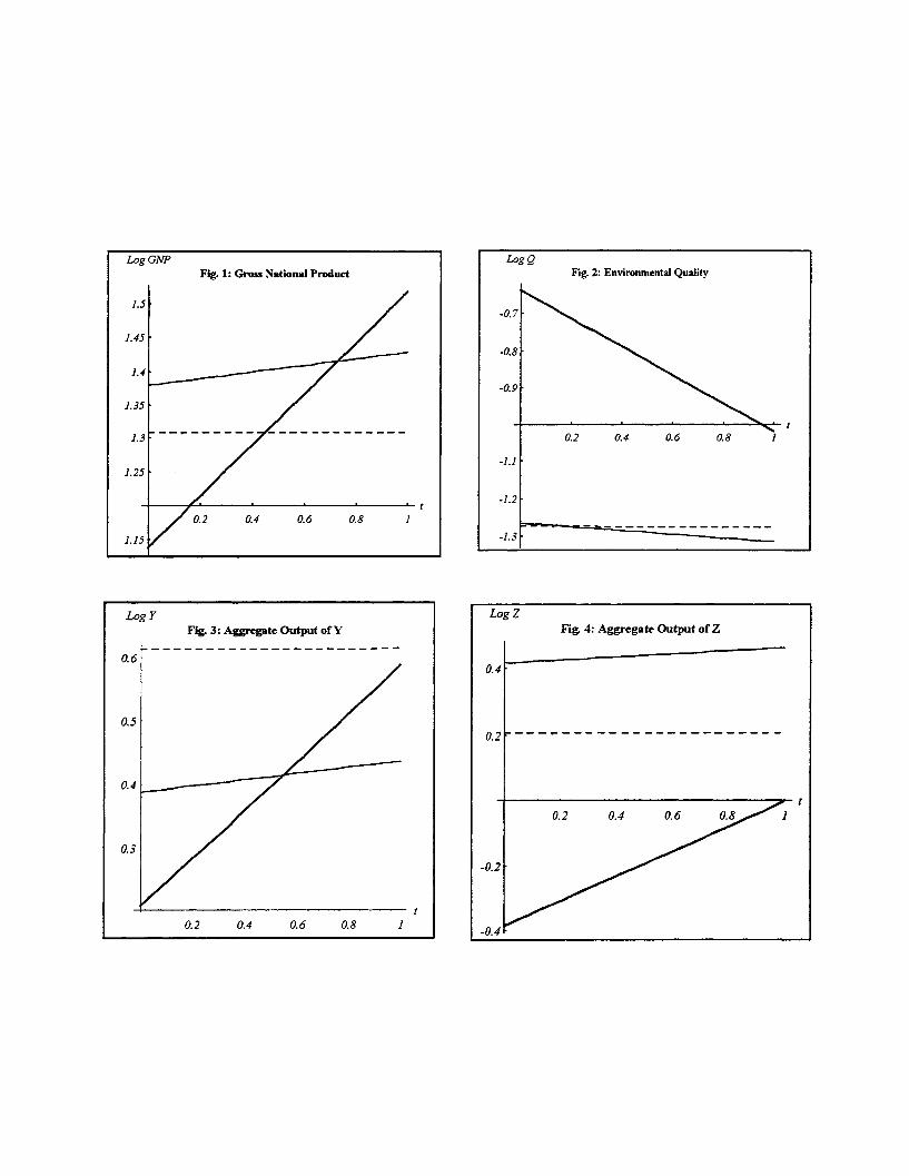
The solutions for some variables of interest are given in Table 2 and their behavior overtime is

depicted in Figures 1-6 in Appendix II. It should be noted that the thick lines represent Pareto optimal

equilibrium, dashed lines stand for autarky equilibrium, and the thick lines denote trade equilibrium.

As expected trade promotes growth since the growth rate under trade is greater than that

under autarky. Both growth rates are, however, smaller than the Pareto optimal rate. Trade worsens

the quality of the environment. This can be seen more clearly from Fig. 2. The overall effects on

welfare of opening the economy to trade are positive: welfare under trade is higher than welfare for

a closed economy. Not surprisingly, welfare is maximized under Pareto equilibrium. Under trade the

economy consumes more than it produces of commodity Y and so imports Y and exports Z.

Figures 7-8 depict the effects of environmental policy on growth. As it is clear from Figure

7, growth increases monotonically with pollution taxes on sector Y. This should be expected in light

of the fact that Y is more capital intensive than Z, and the tax forces it to release more capital so as

to be used in R&D which is capital intensive. An emission tax on sector Z has the opposite effect.

This is clear from Figure 8.

VII. Conclusions

In this paper we have developed an endogenous growth model of a small open economy that

incorporates the welfare effects of environmental quality and its relation to pollution and pollution

abatement activities. Several conclusions emerge from the analysis of this model. First, long-run

growth increases with (i) the country's endowments, (ii) the degree of openness provided whatever

factor intensity R&D has, exportables have less of it than importables, and (iii) the degree of market

power of patents' holders. Second, the effects of the environment on growth depend on the elasticity

28

of intertemporal substitution of consumption. If it is greater than one, environment slows growth. If

it is, however, less than one, environment increases growth. It is worth mentioning that the empirical

literature puts the elasticity ofintertemporal substitution below one. Concerns about the environment

can explain the large differences in growth rates across countries. Third, the effects of trade on

environment and welfare are ambiguous. They depend on price elasticities of supply of traded goods,

the terms of trade effects on growth, and pollution intensities. Numerical exercises, however, suggest

trade worsens the quality of the environment but improves welfare. Fourth, because there is a positive

externality from knowledge creation and negative externality from pollution, the competitive growth

rate can be greater or smaller than the Pareto optimal rate. In one razor edge equilibrium, the two

rates are equal. In the balanced growth equilibrium, the decentralized growth rate is below the Pareto

optimal rate. The market rate of growth is likely to be greater than the optimal rate the larger the

degree of monopoly power and the stronger the effects of environmental externalities. Many policy

instruments can be used to align the two growth paths. The choice of the policy variable depends on

the relationship between the Pareto optimal and market rates of innovation. If the former is greater

than the latter, it is imperative to design policies that increase the profitability ofR&D and decrease

the profitability of sectors which compete more intensively with R&D for resources. We analyzed two

ways in which technological change affects pollution. In the first, technological change increases the

stock of knowledge and that makes it less costly for firms to control pollution. In the second,

technological change augments productivity and hence reduces the need for polluting inputs.

29

Appendix I: The social planner's problem

Case (1): Environmental quality is given by equation (7). In an optimal allocation all the quantities:

X(j), X(j), and Lx(j) will be the same for all i = y, z and j E [O,M]. This enables us to rewrite the social

planner's problem as

Max Jo" V(E,py,p,Q) e-' tdt

s.t.

(2), (3), (6), (7), (26)

Dy + Dz = XM(1i-Y

X = AKx'Lxl,-

L =Ly+ L+ L +Lm

K = K, + Ky+ K, +

M(O) > 0 given.

where L. and K. denote labor and capital used in all intermediate inputs sectors, respectively.

The current value Hamiltonian of this problem can be written as follows

EQ 1-[ _] -1

H = + P.(pyY*+pzZ-E) + PQ(AQY Z - Q) + ry(AyKy 'LyD Y) +1-a

r.(AzKPLP DI-Z) + pd(XM ('Y1 6-D-D) + w(L-LY-L-L-Lm) +

i(K-Ky-K -K -Ka) + xA m K Lm M + x (AKLq - X),

where pN, ry, r px , Pd, Wk, WvL, and X denote the shadow prices associated with the relevant

constraints.

F.O.Cs are

(1) H = p + - = 0

(2) paH + = - rP = 0

dE

(4) M-I =E 1-0Q"(t-o)-- _ .0aQ

rs ryY _ 0ai- rY

aD, D

(6) aH r

8K1 K,rH rY _

(8) = 6 - w = 0(9) aH x (A.l)

SKx KS

(10) = •, - w, = o0

L L0I I

8H rz(12) -a = p (--- - = 0

8 z Lz

(14) = (1-8 )M = 08Lz LZ(14) 7 Lw =aLM LaS 1- _

(15) - = PM -~ =3X(16) i = pX - MD M

& M M

We find it instructive to compare these optimality conditions to some of the competitive equilibrium

conditions. If we substitute the demand for labor and capital from equations (A. 1.5 - A. 1.15) in the

production function for Y, Z, X, and Mi we arrive at the following

6-1 -_-8 - 1-0-" -" : ' (A.2)r, = wk WL Pd r, = WWL P, dP= W 'WL Pd = M X - A.M

Compare these to equations (8), (9), (10'), (11), and (13). We see here the social planner adjust prices

to account for externalities and noncompetitiveness. The noncompetitiveness is corrected for in the

equation for px. Here the marginal cost of producing the X is equated to the shadow price of X. There

is no mark-up over marginal cost as in the market solution. To see more clearly how pollution is

corrected manipulate equations (A. 1.1 - A. 1.4) to get an identity that is valid if

r, = [l1( ey+e)]p.py and r, = [1+(eY+e)p]p.p (A.3)

So, foreign prices of Y and Z are adjusted for pollution externalities.

Let M grows at the constant rate g, and both Y and Z grow at the rate g (not necessarily

constant). The above equations, with the fact that sectoral allocations for labor and capital are

constant in all sectors and equations (A. 1.3), (A. 1.7), and (A. 1.8) imply

WL Wk (A.4)w L w k

where Y = o + (1-o)P.(E+rl) andg is given by

303(1-5)S= ---- g. (A.5)

Equations (A.2), (A.4), and (A.5) can be combined to obtain

. [ - l]gm. (A.6)

Using equations (A.1.5 - A.1.15) in the resource constraints and rearranging gives the national

income as

rYY + rZ + XMg. = wLL +wkJ.

This result with equation (A.5) enables us to rewrite equation (A. 1.16) as

x (1-8)a3 / w ,- = P - - Am-{(L)[L + (-)K]- g }. (A.8)Swk WL

From (A.3) and the cost functions in (A.2) we can obtain (w/wL) = (p/p)1Y"(-p1). Combing equations

(A.6) and (A.8) and making use of this result we arrive at the growth rate of innovation in terms of

the parameters of the model and exogenous variables as given by equation (32) in the text.

Case (2): Environmental quality is given by equation (7). The current value Hamiltonian would be

the same except for one modification: equation (7') requires Q = Aq XlM(E-' ' . The equations that

need to be changed in the F.O.Cs are

(1') OH _

Oy(li = pePy - r O =

(2) H _ PeP- r = Oaz

(15/) OH (Dy Dz) pQ (A.1')(1'6 - = P~d-Px = 0ax x X

-PQ (1-8) (Dy+Dz) PQQ(16) i = p - - Pd

eM M X M

The cost function will be given as before by the equations in (A.2) except for Pd. Using equations

(A. 1.1', 2'), (A. 1.3-6), and (A. 1.15') we get the following relation for pd

Pd = M a (A. 10)«3-P

Since sectorial demands for labor and capital are constant in steady state X is also constant. This

implies that Q grows at (e-1)gn/e. Manipulating equations (A.1.1'), (A.1.2'), (A.1.3), (A.1.4),

(A.7)

differentiating the resulting expression with respect to time, and using the fact that E grows at a 3(1-

8)g/68 with the last result we obtain

.-. -- gM (A.10)

where ' = o -a (1-o)(e-1)8(1-6)Ea3.

equations (A. 1.1') and (A. 1.2') tells us that ry/r = py/p. Using this with the cost functions gives

(wk/WL) = (py/pz)/(• 1 l) . Hence, both wk and wL grow at the same rate which we can obtain by

differentiating equation (A. 1.7) with respect to time and observing that Ky is constant in the steady

state. Thus,

L Wk 3( ) (A. 11)

WL Wk 6

which with the cost function for R&D sector yields

- (1-T')•1- - 1. (A.12)Ix 6

Equation (A. 1.15') can be manipulated as follows. pX = - PQQ + pd(Dy + D) = - pQQ + a3(rY+ rzZ).

But from equations (A.1.1'), (A.1.2'), (A.1.3), and (A.1.4) we get pQQ = gppE = t(ryY+ rZ). Then

pxX = (a 3 - tg)( ryY+ rZ). From the resource constraint we will be able to get: wkwL - XMg =

pxX + (1-a 3 )( ryY+ rzZ) = (1-[)( ryY+ rZ). Using this result in equation (A. 1.16') we get

S,/(WkK +WLL)-- -g- p -g g, (A.13)

where A' = [(E-1)/E + a 3(1-8)/5]/(1-t). Equating (A.12) and (A. 13) and rearranging we obtain the

growth rate as in equations (32') in the text.

Appendix H: Tables and Figures

Table 1: Parameters.

4 p p e , A a a a3 A P P3 3 A2 6

.5 .5 1.2 .47 -.5 -.5 1 .5 .25 .25 2.8 .25 .5 .25 2.8 .2 .1

A, Aw ,, v ,, v ,, A A 0, 6 Am p, p, t,, T, A K L

2 3 .25 .1 .2 .15 1 1 .8 .25 1 1.6 .03 .02 1.3 4 1

Table 2: Steady State Values.

1Variables with superscript 0 are constant over time, with + are growing at the common growth rate, and thosewith a minus superscript are growing at negative the growth rate.

Variables" Autarky Trade Pareto Optimal

Equilibrium Equilibrium Equilibrium

Growth Rateo .00129 .0493 .3805

Output ofY, 1.8467 1.4745 1.2303

Output ofZ, 1.2265 1.5168 .6809

Environmental Qualify .2797 .2823 .5282

GNP + 3.6954 3.9734 3.1194

Emissions from Y '3.5618 2.8139 2.1131

Emissions from Z '3.5869 4.4571 1.6957

Emissions Controlled by Y+ .1316 .135 .3475

Emissions Controlled by Z! .0926 .0932 .3471

Interest Rateo .4716 .5341

Price of Capital+ .2777 .2461

Price of Labor+ 1.5522 1.7726

Price of a New Design0 1.566 1.4698

Consumption ofY+ '1.8467 1.9507 1.1599

Consumption ofZ+ 1.2265 1.2191 .7249

Welfareo -.4934 -.3171 -.0348

Log YFig. 3: Aggregate Output of Y

t

Log ZFig. 4: Aggregate Output of Z

t

0.2 0.4 0.6 0.8 1

I

n~ fl fl ~ fl2

Log EcyFig. 5: Pollution Controlled by Sector Y

-0.8

-1

-1.2

-1.4

-1.6

-1.8

Log EczFig. 6: Pollution Controlled by Sector Z

-0.75

-1

-1.25

-1.5

-1.75

-2.25

0.2 0.4 0.6 0.8 1

GrowthFig. 7: Growth VS Pollution Tax On Sector Y

Towy6 7

GrowthFig. 8: Growth VS Pollution Tax On Sector Z

Towz2 3 4 5

W.1 h %y U. v

-

-I

References

Blitzer, et al. (1993) "Growth and Welfare Losses From Carbon Emissions Restrictions: A GeneralEquilibrium Analysis for Egypt", Energy Journal 14, No. 1, 57-81.

Bovenberg A.L., and S. Smulders (1993) "Environmental Quality and Pollution-Saving TechnologicalChange in a Two-Sector Endogenous Growth Model", Center for Economic Research,Tilburg University, the Netherlands.

Burniaux, J.M., G. Nicoletti, and J. Oliveira-Martins (1992) "GREEN: A Global Model forQuantifying the Costs of Policies to Curb CO2 Emissions", OECD Economic Studies 19, 49-92.

d'Arge, R.C., and K.C. Kogiku (1973) "Economic Growth and the Environment", Review ofEconomic Studies 40, 61-77.

Dixit A., and J. Stiglitz (1977) "Monopolistic Competition and Optimum Product Diversity",American Economic Review 67, 297-308.

Dowing, P.B., and L.J. White (1986) "Innovation in Pollution Control", Journal of EnvironmentalEconomics and Management 13, 18-29.

Elbasha, E. (1995) "Endogenous Growth and the Environment", work in progress.

Ethier, W. (1982) "National and International Returns to scale in the Modem Theory of InternationalTrade", American Economic Review 72, 389-405.

Grossman G., and E. Helpman (1991a) Innovation and Growth in the Global Economy, MIT Press,Cambridge, Mass.

Grossman G., and E. Helpman (1991b) "Growth and Welfare in Small Open Economy" in: E.Helpman and A. Razin, eds., International Trade and Trade Policy, MIT Press, Cambridge,Mass.

Grossman G., and E. Helpman (1994) "Endogenous Innovation in the Theory of Growth", Journalof Economic Perspectives 8, 23-44.

Grossman G., and A. Krueger (1994) "Economic Growth and The Environment", Woodrow WilsonSchool, Princeton University, Princeton, New Jersey.

Grossman G., and A. Krueger (1993) "Environmental Impacts of a North American Free TradeAgreement', in P. Garber, ed., the U.S.-Mexico Free Trade Agreement, MIT Press,Cambridge, Mass., 13-56.

Gruver, G.W. (1976) "Optimal Investment in Pollution Control Capital in a Neoclassical Growth

Context", Journal of Environmental Economics and Management 3, 165-177.

Helpman, E. (1992) "Endogenous Macroeconomic Growth Theory", European Economic Review36, 237-67.

Hoeller, P., A. Dean, and J. Nicolaisen (1991) "Macroeconomic Implications of ReducingGreenhouse Gas Emissions: A survey of Empirical Studies", OECD Economic Studies 16,45-78.

Hung, V., P. Chung, and K. Blackburn (1993) "Endogenous growth, Environment, and R&D",Fondazine Eni Enrico Mattei, Milano, Italy.

Jorgenson, D.W., and P.J. Wilcoxen (1990a) "Environmental Regulation and U.S. EconomicGrowth", The Rand Journal of Economics 21, no. 2, 314-340.

Jorgenson, D.W., and P.J. Wilcoxen (1990b) "Intertemprol General Equilibrium Modelling of U.S.Environmental Regulation", Journal of Policy modeling 12, no. 4, 715-744.

Jorgenson, D.W., and P.J. Wilcoxen (1993a) "Reducing U.S. Carbon Dioxide Emissions: The Costof Alternative Instruments", Journal of Policy Modeling 15, no. 1.

Jorgenson, D.W., and P.J. Wilcoxen (1993b) "Energy, Environment, and Economic Growth", inKneese, A.V. and J.L. Sweeny (1993), eds, Handbook of Natural Resource and EnergyEconomics, vol. III, 1267-1349, Elsevier Science Publishers B.V.

Kaldor, N. (1961) "Capital Accumulation and Economic Growth", in: F. Lutz, ed., The Theory ofCapital, Macmillan, London.

Keeler, E., M. Spence, and R. Zeckhauser (1971) "The Optimal Control of Pollution", Journal ofEconomic Theory 4, 19-34.

Krautkraemer, J.A. (1985) "Optimal Growth, Resource Amenities and Preservation of NaturalEnvironments", Review of Economic Studies 52, 153-170.

Lerner, AP. (1934) "The Concept of Monopoly and the Measurement of Monopoly Power", Reviewof Economic Studies 1, 157-175.

Lucas, R.E. (1993) "Making a Miracle", Econometrica 61, 251-272.

Lucas, RE. (1988) "On the Mechanics of Economic Development", Journal ofMonetary Economics22, 3-42.

Magat, W.A. (1978) "Pollution Control and Technological Advance: A Dynamic Model of the Firm",Journal of Environment Economics and Management 5, 1-25.

Manne, A.S., and R.G. Richels (1992) Buying Greenhouse Insurance, MIT Press, Cambridge, Mass.

Marrewijk, C., F. Ploeg, and J. Verbeek (1993) "Is Growth Bad for the Environment? Pollution,Abatement, and Endogenous Growth", Working Paper, World Bank, Washington, D.C.

Nordhaus, W. (1991a) "To Slow or Not to Slow: The Economics of Greenhouse Effects", TheEconomic Journal 101, no. 6, 920-37.

Nordhaus, W. (199 b) "A Sketch of the Economics of the Greenhouse Effect", American EconomicReview 81, 146-150.

Nordhaus, W. (1992) "An Optimal Transition Path for Controlling Greenhouse Gases", Science 258,1315-1319.

Nordhaus, W. (1993) "How Much Should we Invest In Preserving our Current Climate?, in: Giersch,ed., Economic Progress and Environment Concerns, Springer-Verlag, Berlin.

Rebelo, S. (1991) "Long-Run Policy Analysis and Long-Run Growth", Journal of Political Economy99, 500-521.

Rivera-Batiz, L., and P. Romer (1991) "Economic Integration and Endogenous Growth", QuarterlyJournal of Economics 106, 531-556.

Romer, P. (1986) " Increasing Returns and Long-Run Growth", Journal of Political Economy 94,1002-37.

Romer, P. (1989) "Capital Accumulation in the Theory of Long Growth", in : R. Barro, ed., ModernBusiness Cycle Theory, Harvard University Press, Cambridge, Mass.

Romer, P. (1990) "Endogenous Technological Change", Journal of Political Economy 98, S71-S102.

Romer, P. (1994) "The Origins of Endogenous Growth", Journal of Economic Perspectives 8, 3 -22.

Sala-i-Martin, X. (1990) "Lecture notes on economic growth II", NBER Working Papers No. 3655.

Shafik, N., and S. Bandyopadhyay (1992) "Economic Growth and Environmental Quality: Time-Series and Cross-Country Evidence", Background paper for World Development Report1992, World Bank, Washington D.C.

Solow, R. (1994) "Perspective on Growth Theory", Journal of Economic Perspectives 8, 45 - 54.

Tahvonen, 0., and J. Kuuluvainen (1993) "Economic growth, Pollution, and Renewable Resources",Journal of Environment Economics and Management 24, 101-118.

World Bank (1992) Development and the Environment, World Development Report, OxfordUniversity Press, New York.

RECENT BULLETINS

89-4 Rosenzweig, Mark and Hans Binswanger, "Wealth, Weather Risk and the Composition andProfitability: of Agricultural Investments," June.

89-5 McGuire, Mark F. and Vernon W. Ruttan, "Lost Directions: U.S. Foreign Assistance Policy Since NewDirections," August.

89-6 Coggins, Jay, "On the Welfare Consequences of Political Activity," August.

89-7 Ramaswami, Bharat and Terry Roe, "Incompleteness in Insurance: An Analysis of the MultiplicativeCase," September.

89-8 Rosenzweig, Mark and Kenneth Wolpin, "Credit Market Constraints, Consumption Smoothingand the Accumulation of Durable Production Assets in Low-Income Countries: Investments inBullocks in India," September.

89-9 Pitt, Mark and Mark Rosenzweig, "The Selectivity of Fertility and the Determinants of Human CapitalInvestments: Parametric and Semi-Parametric Estimates," October.

89-10 Ruttan, Vernon, "What Happened to Political Development," November.

90-1 Falconi, Cesar and Terry Roe, "Economics of Food Safety: Risk, Information, and the Demand andSupply of Health," July.

90-2 Roe, Terry and Theodore Graham-Tomasi, "Competition Among Rent Seeking Groups in GeneralEquilibrium," September.

91-1 Mohtadi, Hamid and Terry Roe, "Political Economy of Endogenous Growth," January.

91-2 Ruttan, Vernon W., "The Future of U.S. Foreign Economic Assistance," February.

92-1 Kim, Sunwoong and Hamid Mohtadi, "Education, Job Signaling, and Dual Labor Markets in DdBigCountries," January.

92-2 Mohtadi, Hamid and Sunwoong Kim, "Labor Specialization and Endogenous Growth," January.

92-3 Roe, Terry, "Political Economy of Structural Adjustment: A General Equilibrium - Interest GroupPerspective." April 1992.

92-4 Mohtadi, Hamid and Terry Roe, "Endogenous Growth, Health and the Environment." July 1992.

93-1 Hayami, Yujiro and Vernon W. Ruttan, "Induced Technical and Institutional Change Evaluation andReassessment." February 1993.

93-2 Guyomard, Herv6 and Louis Pascal Mahe, "Producer Behaviour Under Strict Rationing and Quasi-Fixed Factors." September 1993.

94-1 Tsur, Yacov and Amos Zemel, "Endangered Species and Natural Resource Exploitation: Extinction Vs.Coexistence." May 1994.

94-2 Smale, Melinda and Vernon W. Ruttan, "Cultural Endowments, Institutional Renovation and TechnicalInnovation: The Groupements Naam of Yatenga, Burkina Faso." July 1994

94-3 Roumasset, James, "Explaining Diversity in Agricultural Organization: An Agency Perspective." August1994.

95-1 Elbasha, Elamin H. and Terry L. Roe, "On Endogenous Growth: The Implications of EnvironmentalExternalities." February 1995.