On Detectability Of Networked Discrete Event Systems

Wayne State University

Wayne State University Dissertations

1-1-2017

On Detectability Of Networked Discrete EventSystemsYazeed SasiWayne State University,

Follow this and additional works at: http://digitalcommons.wayne.edu/oa_dissertations

Part of the Electrical and Computer Engineering Commons

This Open Access Dissertation is brought to you for free and open access by DigitalCommons@WayneState. It has been accepted for inclusion inWayne State University Dissertations by an authorized administrator of DigitalCommons@WayneState.

Recommended CitationSasi, Yazeed, "On Detectability Of Networked Discrete Event Systems" (2017). Wayne State University Dissertations. 1870.http://digitalcommons.wayne.edu/oa_dissertations/1870

http://digitalcommons.wayne.edu/?utm_source=digitalcommons.wayne.edu%2Foa_dissertations%2F1870&utm_medium=PDF&utm_campaign=PDFCoverPages

http://digitalcommons.wayne.edu/?utm_source=digitalcommons.wayne.edu%2Foa_dissertations%2F1870&utm_medium=PDF&utm_campaign=PDFCoverPages

http://digitalcommons.wayne.edu/oa_dissertations?utm_source=digitalcommons.wayne.edu%2Foa_dissertations%2F1870&utm_medium=PDF&utm_campaign=PDFCoverPages

http://digitalcommons.wayne.edu/oa_dissertations?utm_source=digitalcommons.wayne.edu%2Foa_dissertations%2F1870&utm_medium=PDF&utm_campaign=PDFCoverPages

http://network.bepress.com/hgg/discipline/266?utm_source=digitalcommons.wayne.edu%2Foa_dissertations%2F1870&utm_medium=PDF&utm_campaign=PDFCoverPages

http://digitalcommons.wayne.edu/oa_dissertations/1870?utm_source=digitalcommons.wayne.edu%2Foa_dissertations%2F1870&utm_medium=PDF&utm_campaign=PDFCoverPages

ON DETECTABILITY OF NETWORKED DISCRETE EVENT SYSTEMS

by

YAZEED SASI

DISSERTATION

Submitted to the Graduate School

of Wayne State University,

Detroit, Michigan

in partial fulfillment of the requirements

for the degree of

DOCTOR OF PHILOSOPHY

2017

MAJOR: ELECTRICAL ENGINEERING

Approved By:

______________________________________

Advisor Date

______________________________________

______________________________________

______________________________________

© COPYRIGHT BY

YAZEED SASI

2017

All Rights Reserved

ii

DEDICATION

I dedicate this dissertation to my parents who have worked hard to support me. Also, to all my

siblings and friends.

iii

ACKNOWLEDGEMENTS

I am very fortunate to work under the supervision of Professor Feng Lin, one of the greatest

names in the area of discrete event systems. Professor Lin’s guidance was the candle that led my

way through the Ph.D. journey. Therefore, I am very grateful and thankful for his ultimate support.

Also, I would like to thank my committee members, Associate Professor Caisheng Wang,

Professor Hao Ying, and Professor Nabil Chalhoub, for their valuable comments and suggestions.

I would like also to thank my friend Processor Abdurrahman Hakemi for his support. Also, I want

to thank my friend Saleh Emparik for his support and cheering; you will be always living in my

heart. Finally, special thanks go to my Father, Sasi Omran, the man who is behind me all the time.

https://www.facebook.com/abdurrahman.hakemi

iv

TABLE OF CONTENTS

DEDICATION............................................................................................................................... ii

ACKNOWLEDGEMENTS ........................................................................................................ iii

LIST OF FIGURES .................................................................................................................... vii

LIST OF TABLES ....................................................................................................................... ix

CHAPTER 1 INTRODUCTION ................................................................................................. 1

1.1 Overview of Discrete Event Systems .................................................................................... 2

1.1.1 Modeling of Discrete Event System ............................................................................... 2

1.1.2 Detectability of Discrete Event Systems ........................................................................ 4

1.2 Problems and Motivation ...................................................................................................... 6

1.3 Dissertation Organization ...................................................................................................... 7

CHAPTER 2 RELATED WORK................................................................................................ 9

CHAPTER 3 NETWORKED DISCRETE EVENT SYSTEMS AND OBSERVATION .... 17

3.1 Mathematical Background .................................................................................................. 17

3.2 Network Detectability of Discrete Event Systems .............................................................. 26

3.2.1 Definitions of Network Detectabilities ......................................................................... 28

3.2.2 Checking Network Detectabilities ................................................................................ 29

3.2.3 An Algorithm to Check Network Detectabilities of Discrete Event Systems .............. 34

3.3 An Illustrative Example ...................................................................................................... 36

CHAPTER 4 D-DETECTABILITY OF NETWORKED DISCRETE EVENT SYSTEMS 40

v

4.1 Definitions of Networked D-detectabilities. ....................................................................... 40

4.2 Checking Network D-detectabilities ................................................................................... 42

4.3 An Algorithm to Check Network D-detectabilities of Discrete Event Systems ................. 47

4.4 Illustrative Examples ........................................................................................................... 49

CHAPTER 5 PROPERTIES OF NETWORK DETECTABILITY ...................................... 55

5.1 Properties ............................................................................................................................. 55

5.2 Illustrative Examples ........................................................................................................... 58

CHAPTER 6 I-DETECTABILITY OF NETWORKED DISCRETE EVENT SYSTEMS 61

6.1 Mathematical Background and Network I-observer ........................................................... 62

6.2 Definitions of Network I-Detectabilities ............................................................................. 65

6.3 Checking Network I-detectabilities ..................................................................................... 65

6.3.1 Checking Network I-detectabilities with Observation Losses ..................................... 66

6.3.2 Checking Network I-detectabilities without Observation Losses. ............................... 68

6.4 An Algorithm to Check Network I-detectabilities of Discrete Event Systems with

Observation Losses. .................................................................................................................. 72

CHAPTER 7 NETWORK CO-DETECTABILITY ................................................................ 74

7.1 Mathematical Background .................................................................................................. 75

7.2 Definitions of Network Co-Detectabilities ......................................................................... 77

7.3 Checking Network Co-detectabilities ................................................................................. 78

7.4 An Algorithm to Check Network Co-detectabilities of Discrete Event Systems ............... 80

vi

CHAPTER 8 CONCLUSION .................................................................................................... 82

REFERENCES ............................................................................................................................ 83

ABSTRACT ................................................................................................................................. 95

AUTOBIOGRAPHICAL STATEMENT ................................................................................. 97

vii

LIST OF FIGURES

Figure 1. System classification. ...................................................................................................... 3

Figure 2. Printer as a discrete event system. ................................................................................... 4

Figure 3. A networked discrete event system. ................................................................................ 6

Figure 4. Discrete event system G of Example 2.......................................................................... 24

Figure 5. 𝐺𝐿=LOSS(G) of Example 2 .......................................................................................... 25

Figure 6. Observer 𝐺𝐿, 𝑜𝑏𝑠 = 𝑂𝐵𝑆(𝐺𝐿) of Example 2 ................................................................ 25

Figure 7. Networked observer 𝐺𝐷𝐿, 𝑜𝑏𝑠=DL(OBS(𝐺𝐿)) of Example 2 ...................................... 26

Figure 8. The discrete event system G of Example 3 ................................................................... 36

Figure 9. 𝐺𝐿 = 𝐿𝑂𝑆𝑆(𝐺) of Example 3. ...................................................................................... 37

Figure 10. Observer 𝐺𝐿, 𝑜𝑏𝑠 of the system in Example 3 ............................................................ 37

Figure 11. Networked observer 𝐺𝐷𝐿, 𝑜𝑏𝑠 of the system in Example 3 ........................................ 38

Figure 12. The modified discrete event system G' of Example 3 ................................................. 38

Figure 13. Observer 𝐺′𝐿, 𝑜𝑏𝑠 of the modified system in Example 3 ............................................ 39

Figure 14. Networked observer 𝐺′𝐷𝐿, 𝑜𝑏𝑠 of the modified system in Example 3 ....................... 39

Figure 15. A discrete event system G representing a nuclear reactor ......................................... 49

Figure 16. Automaton 𝐺𝐿 of the system in Example 4 ................................................................. 49

Figure 17. Observer 𝐺𝐿, 𝑜𝑏𝑠 of the system in Example 4 ............................................................ 50

Figure 18. Networked observer 𝐺𝐷𝐿, 𝑜𝑏𝑠 of the system in Example 4 ........................................ 50

Figure 19. Discrete event system G of the factory........................................................................ 51

Figure 20. Networked observer 𝐺𝐷𝐿, 𝑜𝑏𝑠 , for the first few states, with 𝑁 = 1 .......................... 52

Figure 21. Networked observer 𝐺𝐷𝐿, 𝑜𝑏𝑠 , for the first few states, with 𝑁 = 2 .......................... 54

Figure 22. Networked observer 𝐺𝐷𝐿, 𝑜𝑏𝑠𝑁 for N ≥ 2 of Example 6 .......................................... 59

viii

Figure 23. Networked discrete event system G of Example 6 .................................................... 60

Figure 24. Networked observers 𝐺𝐷𝐿, 𝑜𝑏𝑠𝑁 for N=1,2 of Example 6 ........................................ 60

Figure 25. Example 8. ................................................................................................................... 67

Figure 26. Network I-Observer for Example 8. ............................................................................ 68

Figure 27. Network I-Observer for Example 9 N=1. .................................................................... 71

Figure 28. Network I-Observer for Example 9 N=0. .................................................................... 72

ix

LIST OF TABLES

Table 1. Some operations on languages. ....................................................................................... 18

Table 2. Logic connectives. .......................................................................................................... 18

1

CHAPTER 1 INTRODUCTION

Discrete event systems have been studied for more than three decades. During this time,

the theory of discrete event systems has developed in many aspects. Supervisory control is the

main control theory developed for discrete event systems [1-6]. The supervisory control is based

on the concept of controllability and observability. The controllability requires that all events to

be disabled must be controllable [3]. The observability requires that whenever there are two strings

that look the same to the supervisor, the control action after them must be consistent [7].

Controllability and observability characterize the existence condition for a supervisor. Several

extensions to basic supervisory control theory have been investigated [8]. Examples include

decentralized control [2, 9], on-line control [10], limited or variable lookahead control [11], and

robust and adaptive control [12]. In order to control or supervise a discrete event system, we need

to estimate the current state of the system. State estimate problems of discrete event systems are

first investigated by Wonham [13], Ramadge [14], and Ozveren and Willsky [15]. Since then it

has become one of the important problems in discrete event systems. If we cannot determine which

state the system is in, then we want to know the set of all possible state that the system may be in.

We call this set “state estimate”. There are many examples to show the importance of state

estimation. For example, the state estimate of a train is important, if at some point, two trains have

to use the same railroad. We need to make sure that we can accurately estimate the state of each

train (train’s location) in order to avoid collision. Another important application for state

estimation is in medicine, where estimating the disease stage is very important. Therefore, the first

question to ask is: Can we determine which state the system is currently in? If the answer is “no”,

then the second question is: Can we distinguish safe states from unsafe states? Detectability theory

attempts to answer these and other questions. In this dissertation, we investigate detectability of

2

networked discrete event systems, which ensures that the states of a discrete event system can

always be detected when delays and losses are introduced into the system.

1.1 Overview of Discrete Event Systems

1.1.1 Modeling of Discrete Event System

The system can be defined as, according to IEEE Standard Dictionary of Electrical and

Electronic Terms, a set of components act together to perform a specific function not possible with

individual parts [1]. The system in general can classified into dynamic and static systems. In

dynamic systems, the output of the system depends on the past values of input. In contrast, the

output of the system is independent of the previous values of the input in case of static systems.

Dynamic systems can be either time-varying or time-invariant systems. In time-invariant dynamic

systems the output of the systems does not depend on time explicitly. Most of the systems we deal

with in system analysis are classified as time-invariant dynamic systems. Depending on the nature

of the system, time-invariant dynamic systems can be further classified to linear or nonlinear

systems. Furthermore, nonlinear time invariant dynamic systems can be classified to continuous-

state and discrete-state. Figure 1 illustrates system classification.

Discrete event system can be classified as a nonlinear time-invariant dynamic system.

Discrete event system is a system that moves from one state to another when an event occurs.

Discrete event systems are called event driven systems because the system stays in one of its states

until the occurrence of the next event. One of the methods used to describe a discrete event system

is the automaton.

Many systems can be modeled as discrete event systems that consist of discrete states and

discrete events [16-18]. For example, the printer can be in three possible states: working, idle, and

broken-down state. Transition from working state to idle state can happen when the printer finishes

the current task, so we call that the event that causes the printer to change its state form working

3

state to idle state. The transitions between states are called events of the discrete event system. The

system generates infinite sequences of events known as strings. A set of strings is defined as

language. The set of all strings started from the initial state is defined as prefix-closed language.

Likewise, if the language ended in a marked state, we call it marked language.

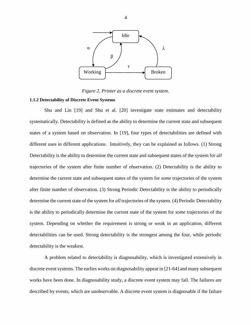
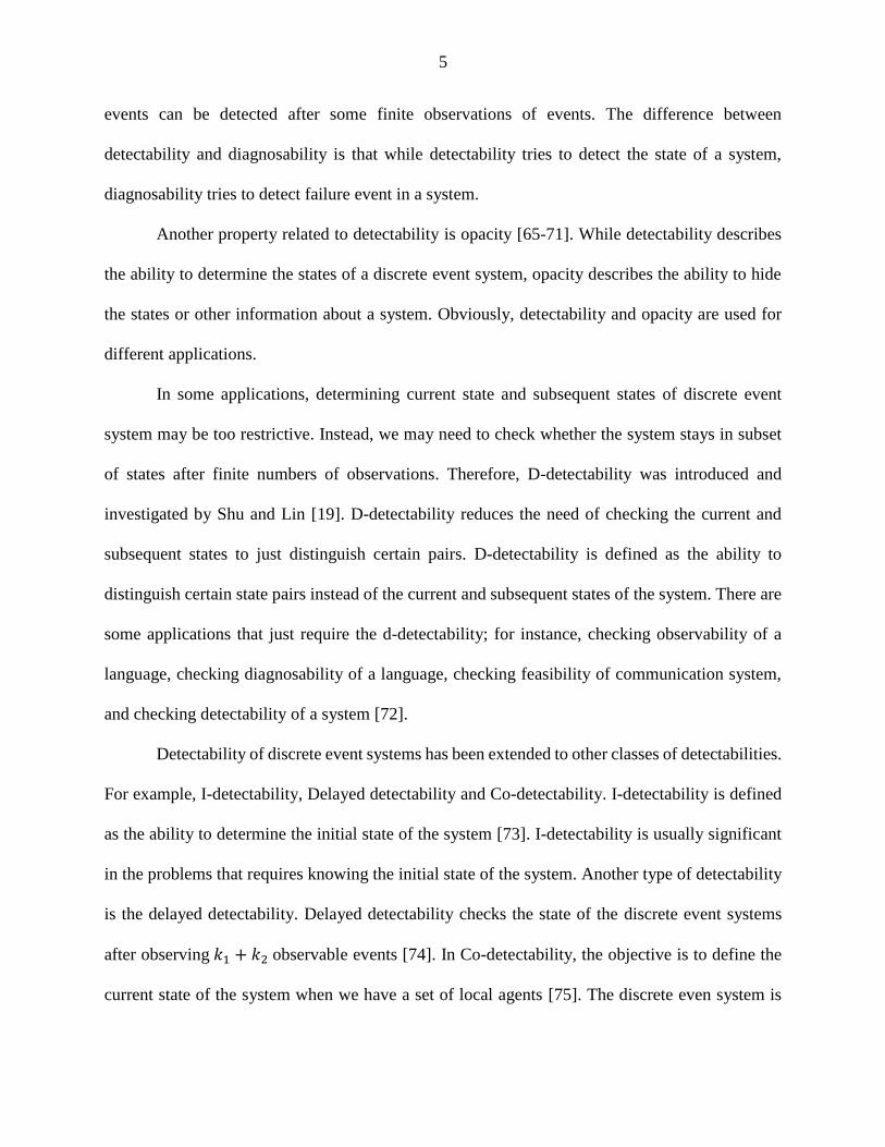
Figure 2 shows how printer can be viewed as a discrete event system. In this discrete event

system, the states are: working state, idle state, and broken state. The events are: 𝛼, 𝛽, 𝜆, and 𝜏.

Figure 1. System classification.

Linear

Time-varying

Systems

Static Dynamic

Time-invariant

Nonlinear

Continuous-

state

Discrete-state

(DES)

4

1.1.2 Detectability of Discrete Event Systems

Shu and Lin [19] and Shu et al. [20] investigate state estimates and detectability

systematically. Detectability is defined as the ability to determine the current state and subsequent

states of a system based on observation. In [19], four types of detectabilities are defined with

different uses in different applications. Intuitively, they can be explained as follows. (1) Strong

Detectability is the ability to determine the current state and subsequent states of the system for all

trajectories of the system after finite number of observation. (2) Detectability is the ability to

determine the current state and subsequent states of the system for some trajectories of the system

after finite number of observation. (3) Strong Periodic Detectability is the ability to periodically

determine the current state of the system for all trajectories of the system. (4) Periodic Detectability

is the ability to periodically determine the current state of the system for some trajectories of the

system. Depending on whether the requirement is strong or weak in an application, different

detectabilities can be used. Strong detectability is the strongest among the four, while periodic

detectability is the weakest.

A problem related to detectability is diagnosability, which is investigated extensively in

discrete event systems. The earlies works on diagnosability appear in [21-64] and many subsequent

works have been done. In diagnosability study, a discrete event system may fail. The failures are

described by events, which are unobservable. A discrete event system is diagnosable if the failure

Idle

Broken Working

α

f β

τ

λ

Figure 2. Printer as a discrete event system.

5

events can be detected after some finite observations of events. The difference between

detectability and diagnosability is that while detectability tries to detect the state of a system,

diagnosability tries to detect failure event in a system.

Another property related to detectability is opacity [65-71]. While detectability describes

the ability to determine the states of a discrete event system, opacity describes the ability to hide

the states or other information about a system. Obviously, detectability and opacity are used for

different applications.

In some applications, determining current state and subsequent states of discrete event

system may be too restrictive. Instead, we may need to check whether the system stays in subset

of states after finite numbers of observations. Therefore, D-detectability was introduced and

investigated by Shu and Lin [19]. D-detectability reduces the need of checking the current and

subsequent states to just distinguish certain pairs. D-detectability is defined as the ability to

distinguish certain state pairs instead of the current and subsequent states of the system. There are

some applications that just require the d-detectability; for instance, checking observability of a

language, checking diagnosability of a language, checking feasibility of communication system,

and checking detectability of a system [72].

Detectability of discrete event systems has been extended to other classes of detectabilities.

For example, I-detectability, Delayed detectability and Co-detectability. I-detectability is defined

as the ability to determine the initial state of the system [73]. I-detectability is usually significant

in the problems that requires knowing the initial state of the system. Another type of detectability

is the delayed detectability. Delayed detectability checks the state of the discrete event systems

after observing 𝑘1 + 𝑘2 observable events [74]. In Co-detectability, the objective is to define the

current state of the system when we have a set of local agents [75]. The discrete even system is

6

called co-detectable if at least one local agent can determine the current state of the system after

finite number of observations. We need Co-detectability when we have distributed systems.

1.2 Problems and Motivation

All detectabilities investigated so far assume that communications between the

agent/supervisor and the plant are reliable and instantaneous. In other words, there is no delay

and/or loss in communication. This assumption may be true for non-networked discrete event

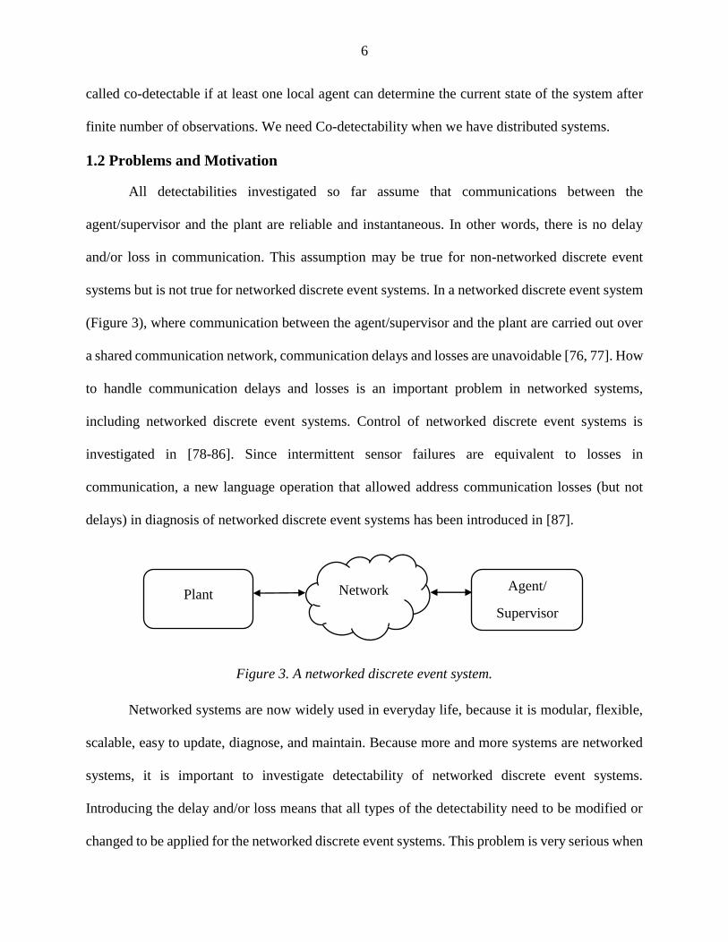
systems but is not true for networked discrete event systems. In a networked discrete event system

(Figure 3), where communication between the agent/supervisor and the plant are carried out over

a shared communication network, communication delays and losses are unavoidable [76, 77]. How

to handle communication delays and losses is an important problem in networked systems,

including networked discrete event systems. Control of networked discrete event systems is

investigated in [78-86]. Since intermittent sensor failures are equivalent to losses in

communication, a new language operation that allowed address communication losses (but not

delays) in diagnosis of networked discrete event systems has been introduced in [87].

Networked systems are now widely used in everyday life, because it is modular, flexible,

scalable, easy to update, diagnose, and maintain. Because more and more systems are networked

systems, it is important to investigate detectability of networked discrete event systems.

Introducing the delay and/or loss means that all types of the detectability need to be modified or

changed to be applied for the networked discrete event systems. This problem is very serious when

Agent/

Supervisor

Plant Network

Figure 3. A networked discrete event system.

7

the supervisor misses to detect an event that may take the whole system to a prohibited state and

cause the system to stop or crash. To prevent unpleasant consequences, we must be able to detect

the discrete event system even under the case of delays and losses.

We assume that the communication channel satisfies FIFO (first in first out) property. In

other words, messages may be delayed, but the order in which they will be received is same as the

order they are sent. This assumption is made in all works in networked discrete event systems. It

is a reasonable assumption if messages are sent using a single channel. On the other hand, if this

assumption is violated, then it will be very difficult, if not impossible, to estimate the state of the

system from the sequence of events observed, because order is most essential in event sequences.

1.3 Dissertation Organization

The remaining dissertation is organized into three chapters and can be summarized as

follows.

In chapter 2, we conduct literature review about what have been done in the area of

detectability of discrete event system to give an idea about the subject.

In chapter 3, we introduced different notations used to formalize networked discrete event

systems. We assume that the systems can be nondeterministic. We also consider both

communication delays and losses. We review how to estimate states under communication delays

and losses. Moreover, we define network detectability and strong network detectability. We derive

necessary and sufficient conditions for network detectability and strong network detectability. We

develop algorithms to check whether a discrete event system is network detectable and/or strongly

network detectable.

In chapter 4, we investigate D-detectability of networked discrete event systems. Four

types of networked D-detectabilities are defined along with the algorithm to check the different

8

types of networked D-detectabilities. We give an example of power distribution system as

networked discrete event system.

In chapter 5, we discuss various properties of networked discrete event systems. We also

give some examples to illustrate these properties. Most of the properties are valid for both

networked detectability and D-detectability.

In chapter 6, we investigate I-detectability of networked discrete event systems. This

chapter consists of four sections. First, mathematical background required for investigating

network I-detectability. Second, definitions of I-detectabilities of networked discrete event

systems. Third, checking I-detectabilities of networked discrete event systems. Last, an algorithm

to check I-detectabilities of networked discrete event systems.

In chapter 7, we study co-detectability of networked discrete event systems. Like chapter

6, this chapter consists of mathematical background required for investigating network co-

detectability, definitions of co-detectabilities of networked discrete event systems, checking I-

detectabilities of networked discrete event systems, and an algorithm to check I-detectabilities of

networked discrete event systems.

In chapter 8, we conclude and summarize our work and point out the main contribution of

our dissertation.

9

CHAPTER 2 RELATED WORK

State estimation problems of discrete event systems was first investigated in 1986 by

Ramadge [14], and since then it becomes one of important problems. Ramadge used a

nondeterministic automaton model for a discrete event system to determine the current state of the

system from a sequence of past events. The scheme has demonstrated valuable in the theoretic

examination of number of fundamental supervisory control issues [88-90]. The motivation to study

state estimation problem for the author came from the importance of state estimate in supervisory

control. In [14], weak observability, strong observability, and coobservability are investigated. In

weak observability, there is no two different states in 𝐺 that have the same sets of event and output

trajectories. Strong observability, on the other hand, is defined as there is no different states in 𝐺

that have common event sequence that can generate a common output sequence [14]. Ramadge

started with a nondeterministic automaton 𝐺 = (𝑄, ∑, 𝛿), which means that the initial state is

unknown. He concluded that pair (G, h) is trackable if for each pair (𝜎, 𝑞) ∈ ∑×𝑄 if 𝑞1, 𝑞2 ∈

𝛿(𝜎, 𝑞) with 𝑞1 ≠ 𝑞2, then h(𝑞1) ≠ h(𝑞2). Therefore, the next state can be uniquely determined

when we know the current state, the next event and the next output. Also, the author introduced

the observation algebra; a subset 𝐴 of 𝑄 is said to be an observation algebra for 𝐺 if for each 𝜎 ∈

∑

𝑆 ∈ 𝐴 implies δ(σ, S) ∈ A

The conception of observation algebra can be used to solve some tracking problems with minimum

of oracle consultations.

In 1988, Caines et al. [91] presented a dynamical logic observer to estimate the current

state of input-state-output automaton. the main reason of the paper is to show that Artificial

Intelligence and Systems and Control Theory are related [92, 93]. The author used simple

10

dynamical systems represented by partially observed automata to explore the state estimation

problems. The state estimations have been constructed from automata using two forms,

construction of classical dynamical system and the construction of dynamical logic system. In

classical dynamical system, the system creates a sequence of state estimates. Dynamical logic

system, on the other hand, creates sequences of propositions that properly describe the properties

of state of the automaton. The paper is basically divided into four main parts. The first part

discusses the dynamical observer problem for finite automata. In this section, a deterministic state

output finite automaton has been used to model the dynamical observers. Moreover, the section

suggests several definitions related to the dynamical observers. The second part of the paper

presents the dynamical logic systems. Also, this section introduces some definitions to define some

properties of the dynamical logic observers. Third section presents the main theorem that links the

observability of input-state-output automaton with the existence of a convergent classical

dynamical observer and the existence of a convergent dynamical logic observer [94]. Furthermore,

this section shows the general design procedure of the classical dynamical observer for the system

output automaton using the notation of DAG observer tree. In the fourth section of the paper, the

authors give an example to explain the state estimation problem using the concepts presented in

their paper. In conclusion, the paper presented a new conception of a dynamic logic systems or

DLS. The paper presented new type of observers, dynamical logic observers. The dynamic logic

observer is a DLS designed to yield a state estimates for dynamic system whose dynamics can be

specified in the dynamical axioms of DLS [91].

In 1990, Özveren and Willsky [15] introduced concepts of observability and resiliency for

discrete event systems [16, 95, 96]. The paper consists of three main sections, and we will try to

briefly summarize these sections. In the first section, the authors presented the mathematical

11

background needed to pursue further in the paper. The authors characterized the notions of state

observability, persistent states and always-observability, indistinguishability, and observability

with delay. Also, the section suggests algorithms to construct suitable observers. The second

section, however, discusses the observer implementation and complexity. The main objective of

this section is to argue the complexity of the constructed observer. The computation complexity

of the observer discussed can be executed polynomial time, but the cardinality of the state space

could be exponential in some cases. The third section of the paper talks about the resiliency of the

observers constructed in section one. For example, the authors wanted to know how resilient the

observer is in case there is an error in the output string we observe. The authors showed that if the

system is observable, then the error propagation will never occur; this means the observer is always

resilient. In summary, the authors had developed polynomial algorithms to check the observability

and build resilient observers; the observer 𝑂𝑅 is always resilient as long as the system is

observable. However, the cardinality of the observer’s state space can be exponential.

In [20] Shu, Lin, and Ying defined the detectability in discrete event systems by the

observation of some event observation and/or some state observation. They assume that the state

of the system is not known in the beginning. Detectability of discrete event systems is very

important especially when it comes to medical application [97, 98]. The paper is divided into two

sections. The first section was to define the basics of the discrete event systems, and how many

system can be modeled by the discrete event systems. The discrete event system is modeled using

automaton of the generator.

𝐺 = (𝑄, ∑, 𝛿)

where 𝑄 is the set of discrete states, ∑ the set of events, and 𝛿: 𝑄× ∑ → 𝑄 the transition function.

As it has been mentioned before, the state estimation used is based on observation of some events

12

and/or some states. The event observation is described projection 𝑃: ∑∗ → ∑𝑜∗ . The output

observation, on the other hand, is described by output map ℎ: 𝑄 → 𝑌. To simplify things, the

authors assume that the automaton G is deadlock free so that at least one event is defined for the

system at any time. The second section of the paper was designated for state estimation and

detectabilities. In this section, the authors defined four properties of the detectabilities. Strong

detectability, weak detectability, strong periodic detectability, and weak periodic detectability

were defined. Moreover, the authors constructed an observer to check the four types of

detectabilities. The observer is used to check detectability through four criterions. The necessary

and sufficient conditions for the four types of detectability were driven and tested by constructing

an observer. The observer constructed has an exponential complexity, so more time is required to

check the detectability of the system.

In [19], Shu and Lin modified the work proposed in [20], and they used a nondeterministic

automaton instead of deterministic automaton. However, [19] presented some extra work; for

example, the authors devolved a technique, which called detector, to check strong detectability

and periodic strong detectability with the polynomial complexity instead of exponential

complexity. Another contribution of [19] was introducing D-detectability, which relaxes the

requirement of estimating the current of the system to just distinguishing certain pairs of state. this

type of detectability is useful in the case where determining the current state and subsequent states

is too restrictive. The paper has three main sections. In the first section, the authors started with

nondeterministic automaton, and they redefined detectability, detectability, strong periodic

detectability, and periodic detectability. The problem of checking these four types of detectability

has been solved by constructing a 𝐺𝑜𝑏𝑠 observer. Constructing 𝐺𝑜𝑏𝑠 can be done by changing all

the unobservable events in the automaton to empty string and converting the nondeterministic

13

automaton to a deterministic automaton. By construction the observer, Shu and Lin checked the

four types of detectabilities. Polynomial algorithms were the main topic for the second section of

the paper. In this section, a detector, 𝐺𝑑𝑒𝑡, for checking detectability was proposed because the

computational complexity of the constructing the observer is exponential. The detector reduces the

computational complexity from exponential to polynomial, and that was a great contribution in

this paper. The last section for this paper was about d-detectability. D-detectability is an extension

of the detectability. In D-detectability, the requirement for determining the current state of the

discrete event system is relaxed to just distinguishing certain pairs of states of the system. The

authors also defined four types of D-detectability (strong D-detectability, D-detectability, strong

periodic D-detectability, and periodic D-detectability). Briefly, the work provided in [19] has

added some extra effort to [20]. For example, a nondeterministic discrete event system automaton

has been used instead of deterministic discrete event system automaton. Also, the computation

complexity of checking strong detectability and strong periodic detectability is reduced to

polynomial by constructing a detector. Another contribution of this paper is introducing D-

detectability, an extended form of detectability.

Shu and Lin also published an IEEE paper [73] in 2013; the paper investigated the initial

state estimation or I-detectability of the discrete event systems. I-detectability defined as the ability

of estimating the initial state of the system. I-detectability is important in some applications such

as offline fault diagnosis [99, 100]. The importance of initial state detectability comes from the

fact that sometimes we may need to determine the state of the system after the occurrence of a

failure, so it would be easy to fix the system. In [73] two types of I-detectabilities are defined:

weak I-detectability and strong I detectability. Besides, I-observer was constructed to check strong

I-detectability and weak I-detectability. Authors also constructed the I-detector to check I-

14

detectability in polynomial complexity. In the first section of the paper, an introduction to the

modeling of the discrete event system has been provided, and definitions for I-detectability are

given. The second section in this paper was about I-observer and I-detector. I-observer has been

constructed to check both types of initial state detectabilities. Because the computational

complexity for I-observer was exponential, I-detector has been also constructed to reduce

complexity to polynomial. However, Constructing I-observer and I-detector are more complex

than constructing 𝐺𝑜𝑏𝑠 and 𝐺𝑑𝑒𝑡 because more modifications are required to be applied to the

discrete event systems. In the last section, the authors introduced closed-loop I-detectability. When

we have weakly I-detectable system, the system is called closed-loop strongly detectable if we can

come up with appropriate controller to attain that. The authors developed an algorithm to check if

the system is closed-loop detectable or not.

In 2013, delayed detectability of discrete event systems was proposed by Shu and Lin in

[74]. The authors extended the detectability problem to delayed detectability. The delayed

detectability investigates system state at event 𝑘1𝑡ℎ after observing 𝑘1 + 𝑘2 observable events.

The paper is divided into four parts. In part one, the authors introduced the discrete event system,

and they used nondeterministic automaton to model the discrete event system. However, there

were two assumptions used to describe the automaton: First, the automaton is deadlock free.

Second, no loops in the automaton contain only unobservable events. Moreover, the authors

defined the delayed detectability, or (𝑘1, 𝑘2)-detectability, as “A discrete event system 𝐺 is

(𝑘1, 𝑘2)-detectable if after 𝑘1 event observations, we can determine the state of the system after

𝑘2 steps of delays for all trajectories” [9]. In the second part of the paper, various properties of

delayed detectability were investigated and proved. Also, in order to check whether the system is

delayed detectable or not, an observer has been constructed to check the delayed detectability.

15

Because the computation complexity of the observer is exponential (bounded by 2|𝑄|), a detector

𝐺𝑑𝑒𝑡 has been constructed. The cardinality of state space of the detector is bounded by |𝑄|2 + 1.

In the third part, however, the authors suggested four algorithms to check whether a system is

(𝑘1, 𝑘2)-detectable or not for a given 𝑘1 and 𝑘2. In the fourth part of the paper, the relation between

delayed detectability with observability, diagnosability, and detectability are discussed. In

summary, the paper investigated the delayed detectability. Also, the authors provided the proofs

for various properties of delayed detectability. Another important contribution for this paper is that

it provided efficient polynomial algorithm to check delayed detectability.

In [75], Shu and Lin investigated co-detectability or decentralized detectability. Co-

detectability is an extension for the detectability. Co-detectability investigates the detectability of

the discrete event systems when we have a set of local agents, and each agent has limited

observations. Co-detectability can be defined as the ability to determine the current state of the

system after limited number of observations using at least one local agent. It is very important to

point out that the agents do not communicate among themselves. There are four types of co-

detectabilities, and they are co-detectability, strong co-detectability, strong periodic co-

detectability, and periodic co-detectability. The paper consists of two parts. The first part was to

introduce and defined each type of co-detectability. For example, co-detectability was defined as

“the discrete event system is called co-detectable if the current state and subsequent states of the

system is known to at least one agent for some trajectories of the systems after finite number of

observations”. In the second part of the paper, a co-observer was introduced to check co-

detectability of the discrete event systems. Based on the co-observer, theorems to check all types

of co-detectabilities of the discrete event systems were introduced. Moreover, the authors

constructed a co-detector to check the strong versions of co-detectabilities in polynomial

16

complexity because the cardinality of the state space of the co-observer is exponential. Overall,

the paper extended the detectability of centralized discrete event systems to decentralized discrete

event systems. Various types of co-detectabilities were defined and checked using co-observer.

Also, to reduce computation complexity, a co-detector was constructed to check strong co-

detectability and strong periodic co-detectability in the polynomial complexity. The author

suggested to investigate the case when there is some communication between the agents as a future

work.

17

CHAPTER 3 NETWORKED DISCRETE EVENT SYSTEMS AND

OBSERVATION

3.1 Mathematical Background

In a networked discrete event system, the agent/supervisor and the plant are connected via

a communication network. We assume that the networked discrete event system is modeled by a

nondeterministic automaton [1, 7, 101]:

𝐺 = (𝑄, ∑, 𝛿, 𝑄0)

where 𝑄 is the finite state set, ∑ is the finite event set, δ：𝑄×∑ → 2𝑄 is nondeterministic transition

function, and 𝑄0 is the set of possible initial state. The language generated by 𝐺 is denoted by 𝐿(𝐺)

[102]. Language is defined as the set of all possible trajectories over ∑. Language is a special type

of set, and all set operations are applicable on the languages. If ∑ = {𝑎, 𝑏, 𝑐}, we can have:

𝐿1 = {휀, 𝑎, 𝑎𝑏𝑏, 𝑏𝑎𝑏𝑏𝑐},

𝐿2 = {𝑎𝑙𝑙 𝑝𝑜𝑠𝑠𝑖𝑏𝑙𝑒 𝑠𝑡𝑟𝑖𝑛𝑔𝑠 𝑜𝑓 𝑙𝑒𝑛𝑔ℎ𝑡 3 𝑤𝑖𝑡ℎ 𝑒𝑣𝑒𝑛𝑡 𝑎} =

{𝑎𝑎𝑎, 𝑎𝑎𝑏, 𝑎𝑎𝑐, 𝑎𝑏𝑎, 𝑎𝑏𝑏, 𝑎𝑏𝑐, 𝑎𝑐𝑎, 𝑎𝑐𝑏, 𝑎𝑐𝑐},

or 𝐿3 = ∑∗ = {휀, 𝑎, 𝑏, 𝑐, 𝑎𝑎, 𝑎𝑏, 𝑎𝑐, 𝑏𝑎, 𝑏𝑏, 𝑏𝑐, 𝑐𝑎, 𝑐𝑏, 𝑐𝑐, … }

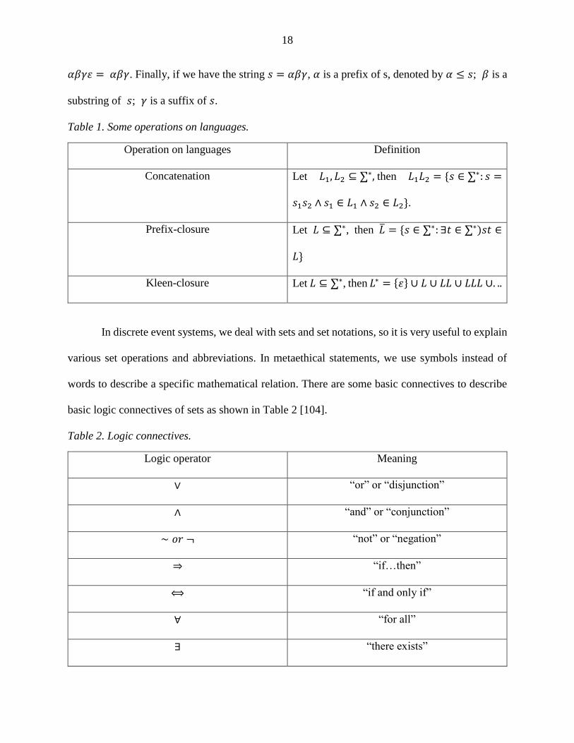
however, there are some operations that apply to just languages, and these include Concatenation,

Prefix-closure, Kleen-closure. Table 1 shows some operations that can be applied to languages.

The events are classified into observable events ∑𝑜 and unobservable events ∑𝑢𝑜. We use

∑∗ to represent all possible strings over ∑. A string is defined as a finite sequence of events [103].

There are some basic operations that can be made over a string. For example, assume we have two

strings 𝛼𝛽𝛾 and 𝛿휂𝜆, then there are some basic operations that can be done of these strings. First,

concatenation of the last two strings will be 𝛼𝛽𝛾𝛿휂𝜆. Second, there is an identity element for any

string, and that element is empty string. Empty string is usually represented by "휀", so 휀𝛼𝛽𝛾 =

18

𝛼𝛽𝛾휀 = 𝛼𝛽𝛾. Finally, if we have the string 𝑠 = 𝛼𝛽𝛾, 𝛼 is a prefix of s, denoted by 𝛼 ≤ 𝑠; 𝛽 is a

substring of 𝑠; 𝛾 is a suffix of 𝑠.

Table 1. Some operations on languages.

Operation on languages Definition

Concatenation Let 𝐿1, 𝐿2 ⊆ ∑∗, then 𝐿1𝐿2 = {𝑠 ∈ ∑∗: 𝑠 =

𝑠1𝑠2 ∧ 𝑠1 ∈ 𝐿1 ∧ 𝑠2 ∈ 𝐿2}.

Prefix-closure Let 𝐿 ⊆ ∑∗, then �̅� = {𝑠 ∈ ∑∗: ∃𝑡 ∈ ∑∗)𝑠𝑡 ∈

𝐿}

Kleen-closure Let 𝐿 ⊆ ∑∗, then 𝐿∗ = {휀} ∪ 𝐿 ∪ 𝐿𝐿 ∪ 𝐿𝐿𝐿 ∪. ..

In discrete event systems, we deal with sets and set notations, so it is very useful to explain

various set operations and abbreviations. In metaethical statements, we use symbols instead of

words to describe a specific mathematical relation. There are some basic connectives to describe

basic logic connectives of sets as shown in Table 2 [104].

Table 2. Logic connectives.

Logic operator Meaning

∨ “or” or “disjunction”

∧ “and” or “conjunction”

∼ 𝑜𝑟 ¬ “not” or “negation”

⇒ “if…then”

⟺ “if and only if”

∀ “for all”

∃ “there exists”

19

∈ “belongs to”

∉ “does not belong to”

− “difference”

⊂ “subset”

|𝑠𝑒𝑡| “cardinality”

|𝑠𝑡𝑟𝑖𝑛𝑔| “length of string”

∪ “union”

∩ “intersection”

× “product”

2𝐴 “power set”

∅ “empty set”

There are some properties of empty string "휀" and empty set

∅. We can summaries these properties as shown below [1]:

1. The empty string does not belong to the empty set, that is,

휀 ∉ ∅.

2. {휀} is a nonempty language that contain just empty string, that is, ∅ ≠ {휀}.

3. ∅∗ = {휀}, and {휀} = {휀}∗.

4. If 𝐿 = ∅ then �̅� = ∅ (𝐿 = ∅ ⇒ �̅� = ∅), also 𝐿 = ∅ ⇔ �̅� = ∅ is true.

5. If 𝐿 ≠ ∅ then 휀 ∈ �̅� (𝐿 ≠ ∅ ⇒ 휀 ∈ �̅�), also (𝐿 ≠ ∅ ⇔ 휀 ∈ �̅�) is true.

Because we deal with sets when we deal with discrete event systems, it is important to

mention basic set axioms. There are six axioms of set theory. These axioms can be summarize as

following [104]:

20

1. The axiom of containment: if all elements in a set 𝐴 is also elements in set 𝐵, then 𝐴 is a

subset of 𝐵 denoted as 𝐴 ⊂ 𝐵,

𝐴 ⊂ 𝐵 ⟺ ∀𝑎(𝑎 ∈ 𝐴 ⇒ 𝑎 ∈ 𝐵).

It is important to mention that any set is a subset of itself.

2. The axiom of extension: two sets, 𝐴 and 𝐵, are equal if and only if each both sets have the

same elements:

𝐴 = 𝐵 ⟺ ∀𝑥((𝑥 ∈ 𝐴 ⟹ 𝑥𝐵) ∧ (𝑥 ∈ 𝐵 ⟹ 𝑥 ∈ 𝐴)).

3. The axiom of intersection: for any two sets, 𝐴 and 𝐵, the class of elements that are in

belonging to both sets 𝐴 and 𝐵 is also a set:

∀(𝐴, 𝐵) ∃ 𝑀 (𝑦 ∈ 𝑀 ⟺ 𝑦 ∈ 𝐴 ∧ 𝑦 ∈ 𝐵).

4. The axiom of union: for any two sets, 𝐴 and 𝐵, the class of elements that belonging to either

𝐴 or to 𝐵 is also a set:

∀(𝐴, 𝐵) ∃ 𝑀 (𝑦 ∈ 𝑀 ⟺ 𝑦 ∈ 𝐴 ∨ 𝑦 ∈ 𝐵).

5. The empty set: the empty set is a set that has no elements. It also called null or void set. We

denote that set by ∅.

6. Power set axiom: for a set 𝐶, there is a special class, the collection of all subsets of the set 𝐶.

∀𝐶 ∃ 𝑃(𝐶)(∀𝐵((𝐵 ∈ (𝑃(𝐶)) ⟺ (𝐵 ⟺ 𝐴)))

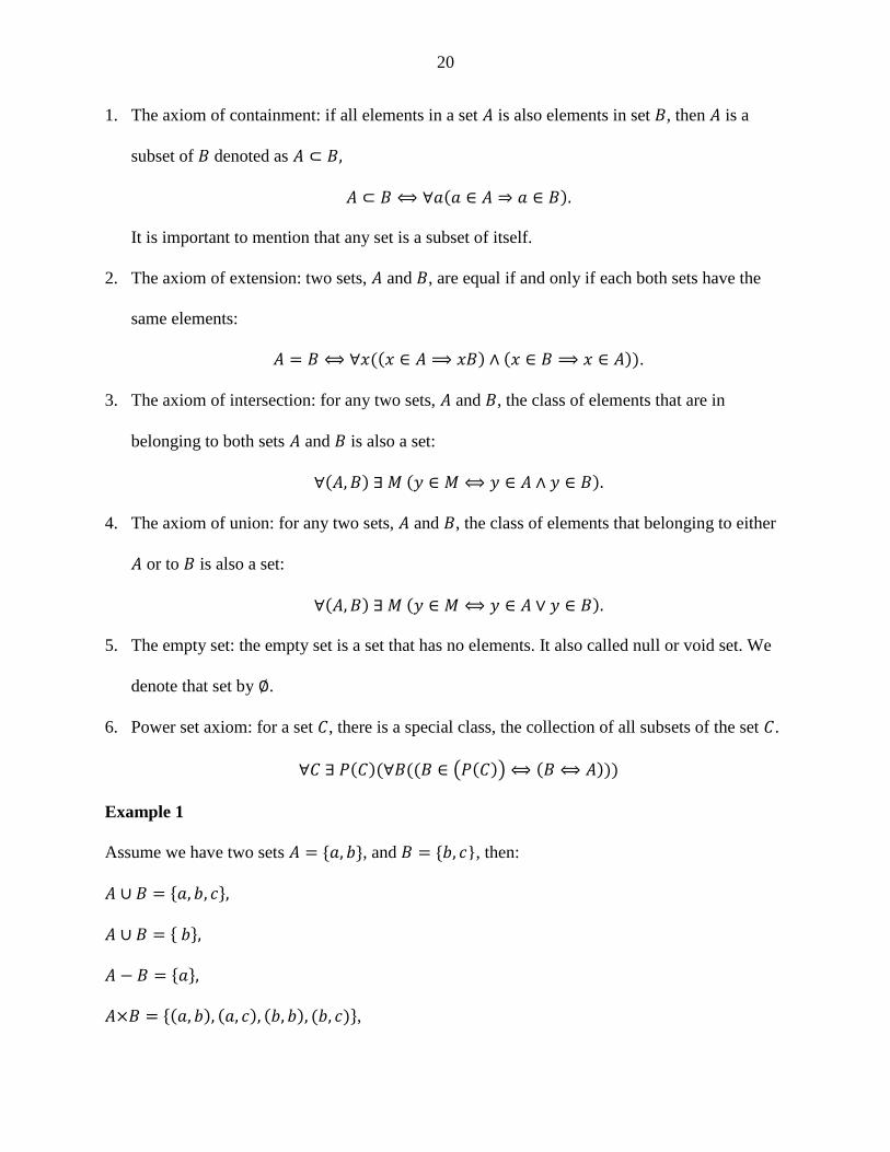
Example 1

Assume we have two sets 𝐴 = {𝑎, 𝑏}, and 𝐵 = {𝑏, 𝑐}, then:

𝐴 ∪ 𝐵 = {𝑎, 𝑏, 𝑐},

𝐴 ∪ 𝐵 = { 𝑏},

𝐴 − 𝐵 = {𝑎},

𝐴×𝐵 = {(𝑎, 𝑏), (𝑎, 𝑐), (𝑏, 𝑏), (𝑏, 𝑐)},

21

|𝐴×𝐵| = 4,

and 2𝐴 = {∅, {𝑎}, {𝑏}, {𝑎, 𝑏}}.

Another type of operation that can be done over strings and languages is projection or

natural projection. Given a large set of events ∑𝑙 and small sets of events ∑𝑠 such that ∑𝑠 ⊂ ∑𝑙.

Projection on strings is a mapping from large set of events ∑𝑙 to small set of events ∑𝑠 [1].

𝑃: ∑𝑙∗ → ∑𝑠

∗

where

𝑃(휀) = 휀

𝑃(𝜎) = {𝜎 if 𝜎 ∈ ∑𝑠

휀 if 𝜎 ∈ ∑𝑙 − ∑𝑠

𝑃(𝑠𝜎)= 𝑃(𝑠)𝑃(𝜎)

Projection deletes all the events that do not belong to the small event set ∑𝑠. If ∑𝑙 = {𝛼, 𝛽, 𝜇},

∑𝑠 = {𝛼, 𝛽}, and 𝐿 = {𝜇, 𝜇𝛽𝛼𝛽, 𝛽𝜇𝛽𝛼𝛽𝜇𝛽}, then 𝑃(𝐿) = {휀, 𝛽𝛼𝛽, 𝛽𝛽𝛼𝛽𝛽}.

The inverse projection can be defined as 𝑃−1(𝑡) = {𝑠 ∈ ∑𝑙∗ ∶ 𝑃(𝑠) = 𝑡}. There are several

properties for projection (𝑃) and invers projection (𝑃−1) that can be summarize in the following

[1]:

1. 𝑃(𝑃−1(𝐿)) = 𝐿

2. 𝐿 ⊆ 𝑃(𝑃−1(𝐿))

3. 𝑃(𝐴 ∪ 𝐵) = 𝑃(𝐴) ∪ 𝑃(𝐵)

4. 𝑃(𝐴 ∩ 𝐵) ⊆ 𝑃(𝐴) ∩ 𝑃(𝐵)

5. 𝑃−1(𝐴 ∪ 𝐵) = 𝑃−1(𝐴) ∪ 𝑃−1(𝐵)

6. 𝑃−1(𝐴 ∩ 𝐵) = 𝑃−1(𝐴) ∩ 𝑃−1(𝐵)

7. 𝑃(𝐴𝐵) = 𝑃(𝐴)𝑃(𝐵)

22

8. 𝑃−1(𝐴𝐵) = 𝑃−1(𝐴)𝑃−1(𝐵)

9. 𝐴 ⊆ 𝐵 ⇒ 𝑃(𝐴) ⊆ 𝑃(𝐵) ∧ 𝑃−1(𝐴) ⊆ 𝑃−1(𝐵)

We used δ to denote the set of all transitions in 𝐺: 𝛿 = {(𝑞, 𝜎, 𝑞′): 𝑞′ ∈ 𝛿(𝑞, 𝜎)}. The set

of observable transitions is denoted by 𝛿𝑜 = {(𝑞, 𝜎, 𝑞′) ∈ 𝛿: 𝜎 ∈ ∑𝑜} . The set of unobservable

transitions is denoted by 𝛿𝑢𝑜 = {(𝑞, 𝜎, 𝑞′) ∈ 𝛿: 𝜎 ∈ ∑𝑢𝑜} . Some observable transitions may be

lost in communication. These transitions are denoted by 𝛿𝐿 (δ𝐿 ⊆ δ𝑜) [79, 103].

We denote the observation mapping under the communication losses by 휃𝐿. After

occurrence of the string 𝑠 in the system, the agent/supervisor will observe 휃𝐿(𝑠). Assume the

string 𝑠 = 𝜎1 … 𝜎𝑖 … 𝜎𝑘, 휃𝐿(𝑠) is obtained by replacing 𝜎𝑖 with empty string (ε) if the

corresponding transition is (𝑞𝑖, 𝜎𝑖, 𝛿(𝑞𝑖, 𝜎𝑖)) ∈ 𝛿𝑢𝑜, with 𝜎𝑖 if (𝑞𝑖, 𝜎𝑖, 𝛿(𝑞𝑖, 𝜎𝑖)) ∈ 𝛿𝑜 − 𝛿𝐿, and

with ε or 𝜎𝑖 if (𝑞𝑖, 𝜎𝑖, 𝛿(𝑞𝑖, 𝜎𝑖)) ∈ 𝛿𝐿. Since 휃𝐿(𝑠) is not unique, 휃𝐿 is the mapping from 𝐿(𝐺) to

2∑0∗ [79]:

휃𝐿: 𝐿(𝐺) → 2∑0∗.

We denote the delayed observation with delays bounded by N steps as 휃𝐷𝑁. For sting 𝑠 ∈ 𝐿(𝐺)

휃𝐷𝑁(𝑠) = {𝑠−𝑖: 𝑖 = 0,1 … , 𝑁},

where 𝑠−𝑖 is the prefix of 𝑠 with the last 𝑖 events removed. If a string 𝑠 ∈ 𝐿(𝐺) occurred,

observation delays will change 𝑠 to one of the strings in 휃𝐷𝑁(𝑠), because the last events may not be

observed yet. 휃𝐷𝑁 is not a unique [79], that is

휃𝐷𝑁: ∑∗ → 2∑∗

.

We will remove superscript 𝑁 if it is understood: 휃𝐷 = 휃𝐷𝑁. With both communication delays and

losses, the observation mapping is described by the composition of 휃𝐿 and 휃𝐷 , denoted as 휃𝐷𝐿

[79]:

휃𝐷𝐿 = 휃𝐿 ∘ 휃𝐷.

23

After observing a string 𝑡, the set of all possible states that the system may be in is called state

estimate after 𝑡, which is defined as follows.

𝐸(𝑡) = {𝑞 ∈ 𝑄: (∃𝑠 ∈ 𝐿(𝐺))𝑡 ∈ 휃𝐷𝐿(𝑠) ∧ 𝛿(𝑞0, 𝑠) = 𝑞}

To obtain state estimate, we do the following. We first construct automaton 𝐺𝐿 to describe the

communication losses [79]:

𝐺𝐿 = 𝐿𝑂𝑆𝑆(𝐺) = (𝑄, ∑0, 𝛿𝑙𝑜𝑠𝑠, 𝑄0),

where 𝛿𝑙𝑜𝑠𝑠 = {(𝑞, 𝜎, 𝑞′): (𝑞, 𝜎, 𝑞′) ∈ 𝛿𝑜} ∪ {(𝑞, 휀, 𝑞′): (𝑞, 𝜎, 𝑞′) ∈ 𝛿𝑢𝑜 ∪ 𝛿𝐿}.

From 𝐺𝐿, we can build the observer 𝐺𝐿,𝑜𝑏𝑠 as

𝐺𝐿,𝑜𝑏𝑠 = 𝑂𝐵𝑆(𝐺𝐿) = (𝑋, ∑0, 𝜉, 𝑥0) = 𝐴𝑐(2𝑄 , ∑0, 𝜉, 𝑈𝑅({𝑄0})).

where 𝐴𝑐(. ) denotes the accessible part, state 𝑥 ∈ 𝑋 is a subset of 𝑄, and 𝑥0 = 𝑈𝑅({𝑄0}) is the

unobservable reach of 𝑄0, defined as

𝑈𝑅(𝑥) = {𝑞 ∈ 𝑄: (∃𝑞′ ∈ 𝑥)𝑞 ∈ 𝛿(𝑞′, 휀)}.

The transition function is defined as

𝜉(𝑥, 𝜎) = 𝑈𝑅({𝑞 ∈ 𝑄: (∃𝑞′ ∈ 𝑥)𝑞 ∈ 𝛿(𝑞′, 𝜎)}).

Next, we extend each state 𝑥 ∈ 𝑋 to 𝑦 = 𝑅(𝑥). 𝑅(𝑥) denotes the set of states that can be reached

within N steps in G, that is,

𝑅(𝑥) = {𝑞 ∈ 𝑄: (∃𝑞′ ∈ 𝑥)(∃𝑠 ∈ ∑∗)|𝑠| ≤ 𝑁 ∧ 𝛿(𝑞′, 𝑠) = 𝑞}

Finally, the networked observer is defined as

𝐺𝐷𝐿,𝑜𝑏𝑠 = 𝐷𝐿(𝑂𝐵𝑆(𝐺𝐿)) = (𝑌, ∑0, 휁, 𝑦0).

In 𝐺𝐷𝐿,𝑜𝑏𝑠, the state set 𝑌 is defined as follows. Denote 𝑋 = {𝑥1, 𝑥2, 𝑥3, … … 𝑥𝑚}, then 𝑌 =

{𝑦1, 𝑦2, 𝑦3, … … 𝑦𝑚} with 𝑦𝑖 = 𝑅(𝑥𝑖). The transition function 휁: 𝑌×∑0 → 𝑌 is defined for 𝑦𝑖, 𝑦𝑗 ∈

𝑌 and ∈ ∑0, as

휁 = {(𝑦𝑖, 𝜎, 𝑦𝑗): (𝑥𝑖 , 𝜎, 𝑥𝑗) ∈ 𝜉}

24

The networked observer can be used to find state estimates. In fact, it is proven in [79]

that

𝐸(𝑡) = 휁(𝑦0, 𝑡)

As in [19, 20, 73], we accept the following assumption

[1] The networked discrete event system 𝐺 is deadlock free [73]

(∀𝑞 ∈ 𝑄)(∃𝜎 ∈ ∑)𝛿(𝑞, 𝜎)!

This means that for any state there is at least one event is defined.

[2] No loops in 𝐺 that contain only unobservable events [73]

¬(∃𝑞 ∈ 𝑄)(∃𝑠 ∈ ∑𝑢𝑜∗ )𝑠 ≠ 휀 ∧ 𝑞 ∈ 𝛿(𝑞, 𝑠).

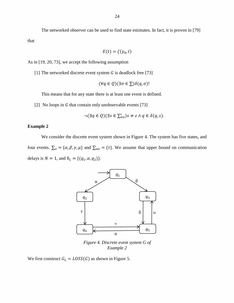
Example 2

We consider the discrete event system shown in Figure 4. The system has five states, and

four events. ∑𝑜 = {𝛼, 𝛽, 𝛾, 𝜇} and ∑𝑢𝑜 = {𝜏}. We assume that upper bound on communication

delays is 𝑁 = 1, and δ𝐿 = {(𝑞1, 𝛼, 𝑞2)}.

We first construct 𝐺𝐿 = 𝐿𝑂𝑆𝑆(𝐺) as shown in Figure 5.

τ

α

γ

β

α

𝑞1

𝑞3 𝑞2

𝑞5 𝑞4

β

µ

Figure 4. Discrete event system G of

Example 2

25

We then construct the observer 𝐺𝐿,𝑜𝑏𝑠 = 𝑂𝐵𝑆(𝐺𝐿) as shown in Figure 6. In 𝐺𝐿,𝑜𝑏𝑠,

𝑋 = {{𝑞1, 𝑞2, 𝑞4}, {𝑞2, 𝑞4}, {𝑞3}, {𝑞4}, {𝑞5}}.

Finally, we construct the networked observer as shown in Figure 7. In 𝐺𝐷𝐿,𝑜𝑏𝑠,

𝑌 = {{𝑞1, 𝑞2, 𝑞3, 𝑞4, 𝑞5}, {𝑞2, 𝑞4, 𝑞5}, {𝑞3, 𝑞4, 𝑞5}, {𝑞3, 𝑞5}, {𝑞4, 𝑞5}}.

α γ

α β

𝑞1, 𝑞2, 𝑞4

𝑞3 𝑞2, 𝑞4

𝑞5

𝑞4

γ

γ

β

µ

ε

α

γ

β

α

𝑞1

𝑞3 𝑞2

𝑞5 𝑞4

β

µ

ε

Figure 5. 𝐺𝐿=LOSS(G) of Example 2

Figure 6. Observer 𝐺𝐿,𝑜𝑏𝑠 = 𝑂𝐵𝑆(𝐺𝐿) of

Example 2

26

Form the networked observer, we know that, for example, if 𝑡 = 𝛼𝜈µ is observed, then the

state estimate

𝐸(𝑡) = 휁(𝑦0, 𝑡) = {𝑞3, 𝑞5}.

3.2 Network Detectability of Discrete Event Systems

Determining the state of a discrete event system is very important, and it is needed in many

applications. The importance of the detectability of discrete event systems varies depending on the

type of the system. For example, detecting the current state of nuclear reactor is more important

than detecting the current state of a printer. The detectability that has been discussed in many

papers is non-networked detectability. In other words, there are no delay and loss involved in the

discrete event system. In the practical systems, delay or loss of the events or control commands

may occur especially when we have networked discrete event systems. Taking the delay and loss

in consideration, we need to redefine the four types of detectabilities: detectability, strong

detectability, periodic detectability, and strong periodic detectability.

α γ

α β

𝑞1, 𝑞2, 𝑞3, 𝑞4, 𝑞5

𝑞3, 𝑞5 𝑞2, 𝑞4, 𝑞5

𝑞3, 𝑞4, 𝑞5

𝑞4, 𝑞5

γ

γ

β

µ

Figure 7. Networked observer

𝐺𝐷𝐿,𝑜𝑏𝑠=DL(OBS(𝐺𝐿)) of Example 2

27

Detectability of discrete event systems was first studied in the mid of 80s in [14, 91]. In

these papers, problems like current state and initial state estimation have been introduced and

studied. In the 1990, the stability current state detectability was studied by [15]. Many papers have

been published after that in [19, 20, 73, 79], and various estimation problems have been discussed.

For example, the four types of detectability, generalized detectability, D-detectability, I-

detectability are investigated in these published papers.

The delay and loss in the events or control commands happen when we have a networked

discrete event system because of the real-time network used to connect the entire system nodes.

There are many advantages of using the networked control systems, such as reducing the

complexity of the system, increasing the simplicity of the system by making it easy to add/remove

nodes, and simplifying the test/diagnose of the system. However, networked discrete event systems

introduce delay and loss, so modifications are made to redefine the detectability in networked

discrete event systems.

The applications usually define what type of detectability we need to use. For example,

defining the current state and subsequent states of the system is required in applications like

monitoring the nuclear reactor’s state, so that we prevent the reactor to access to undesired or

unwanted state.

In this section, we define and investigate detectability of networked discrete event systems,

called network detectability. Depending on the requirements of applications, we consider four

types of network detectabilities: strong network detectability, strong periodic network

detectability, (weak) periodic network detectability, and (weak) network detectability.

We will use the following notations in our work: The set of all possible infinite

strings/trajectories of 𝐺 is denoted by 𝐿𝜔(𝐺) [19, 102]. For a string 𝑠 ∈ 𝐿𝜔(𝐺), we denote the set

28

of all its prefixes by 𝑃𝑟(𝑠). Also, for any finite string 𝑤, we use |𝑤| to denote the length of this

string. For any set 𝑋, we use |𝑋| to denote the number of elements in 𝑋 (cardinality).

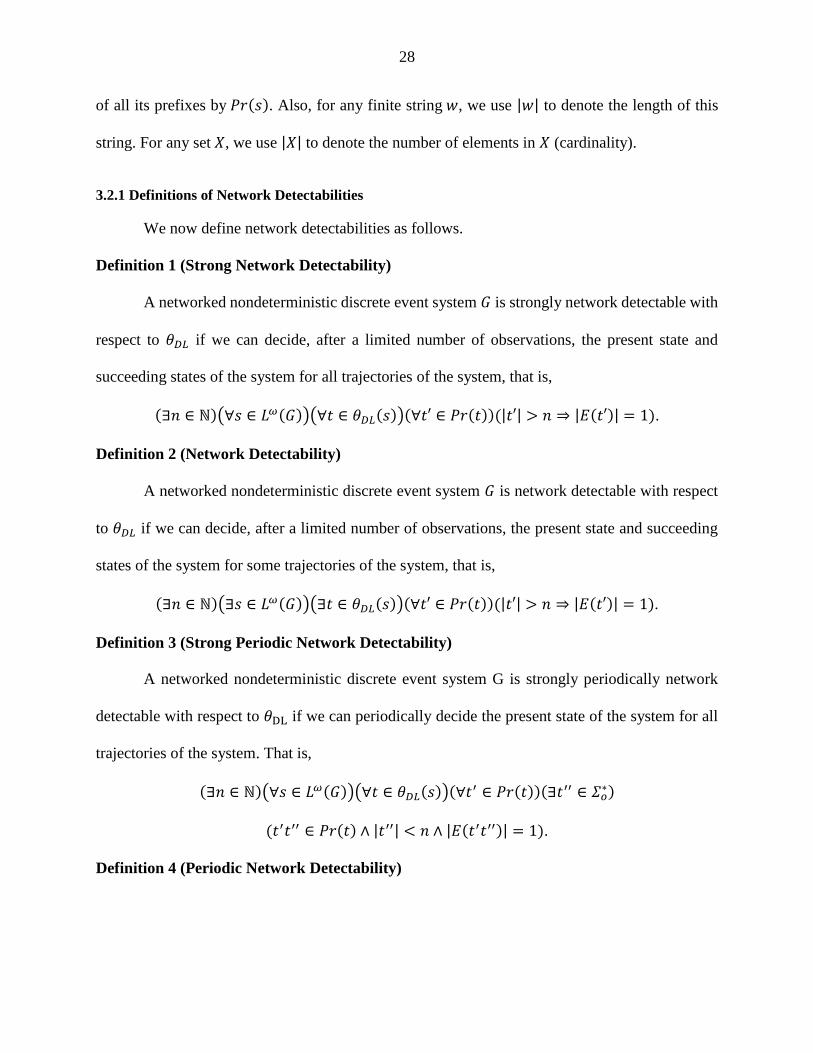
3.2.1 Definitions of Network Detectabilities

We now define network detectabilities as follows.

Definition 1 (Strong Network Detectability)

A networked nondeterministic discrete event system 𝐺 is strongly network detectable with

respect to 휃𝐷𝐿 if we can decide, after a limited number of observations, the present state and

succeeding states of the system for all trajectories of the system, that is,

(∃𝑛 ∈ ℕ)(∀𝑠 ∈ 𝐿𝜔(𝐺))(∀𝑡 ∈ 휃𝐷𝐿(𝑠))(∀𝑡′ ∈ 𝑃𝑟(𝑡))(|𝑡′| > 𝑛 ⇒ |𝐸(𝑡′)| = 1).

Definition 2 (Network Detectability)

A networked nondeterministic discrete event system 𝐺 is network detectable with respect

to 휃𝐷𝐿 if we can decide, after a limited number of observations, the present state and succeeding

states of the system for some trajectories of the system, that is,

(∃𝑛 ∈ ℕ)(∃𝑠 ∈ 𝐿𝜔(𝐺))(∃𝑡 ∈ 휃𝐷𝐿(𝑠))(∀𝑡′ ∈ 𝑃𝑟(𝑡))(|𝑡′| > 𝑛 ⇒ |𝐸(𝑡′)| = 1).

Definition 3 (Strong Periodic Network Detectability)

A networked nondeterministic discrete event system G is strongly periodically network

detectable with respect to 휃DL if we can periodically decide the present state of the system for all

trajectories of the system. That is,

(∃𝑛 ∈ ℕ)(∀𝑠 ∈ 𝐿𝜔(𝐺))(∀𝑡 ∈ 휃𝐷𝐿(𝑠))(∀𝑡′ ∈ 𝑃𝑟(𝑡))(∃𝑡′′ ∈ 𝛴𝑜∗)

(𝑡′𝑡′′ ∈ 𝑃𝑟(𝑡) ∧ |𝑡′′| < 𝑛 ∧ |𝐸(𝑡′𝑡′′)| = 1).

Definition 4 (Periodic Network Detectability)

29

A networked nondeterministic discrete event system G is periodically network detectable

with respect to 휃DL if we can periodically decide the present state of the system for some

trajectories of the system. That is,

(∃𝑛 ∈ ℕ)(∃𝑠 ∈ 𝐿𝜔(𝐺))(∃𝑡 ∈ 휃𝐷𝐿(𝑠))(∀𝑡′ ∈ 𝑃𝑟(𝑡))(∃𝑡′′ ∈ 𝛴𝑜∗)

(𝑡′𝑡′′ ∈ 𝑃𝑟(𝑡) ∧ |𝑡′′| < 𝑛 ∧ |𝐸(𝑡′𝑡′′)| = 1).

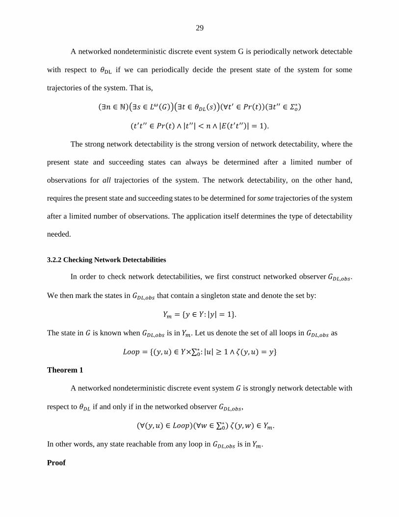
The strong network detectability is the strong version of network detectability, where the

present state and succeeding states can always be determined after a limited number of

observations for all trajectories of the system. The network detectability, on the other hand,

requires the present state and succeeding states to be determined for some trajectories of the system

after a limited number of observations. The application itself determines the type of detectability

needed.

3.2.2 Checking Network Detectabilities

In order to check network detectabilities, we first construct networked observer 𝐺𝐷𝐿,𝑜𝑏𝑠.

We then mark the states in 𝐺𝐷𝐿,𝑜𝑏𝑠 that contain a singleton state and denote the set by:

𝑌𝑚 = {𝑦 ∈ 𝑌: |𝑦| = 1}.

The state in 𝐺 is known when 𝐺𝐷𝐿,𝑜𝑏𝑠 is in 𝑌𝑚. Let us denote the set of all loops in 𝐺𝐷𝐿,𝑜𝑏𝑠 as

𝐿𝑜𝑜𝑝 = {(𝑦, 𝑢) ∈ 𝑌×∑0∗ : |𝑢| ≥ 1 ∧ 휁(𝑦, 𝑢) = 𝑦}

Theorem 1

A networked nondeterministic discrete event system 𝐺 is strongly network detectable with

respect to 휃𝐷𝐿 if and only if in the networked observer 𝐺𝐷𝐿,𝑜𝑏𝑠,

(∀(𝑦, 𝑢) ∈ 𝐿𝑜𝑜𝑝)(∀𝑤 ∈ ∑0∗ ) 휁(𝑦, 𝑤) ∈ 𝑌𝑚.

In other words, any state reachable from any loop in 𝐺𝐷𝐿,𝑜𝑏𝑠 is in 𝑌𝑚.

Proof

30

Note that

(∃𝑛 ∈ ℕ)(∀𝑠 ∈ 𝐿𝜔(𝐺))(∀𝑡 ∈ 휃𝐷𝐿(𝑠))(∀𝑡′ ∈ 𝑃𝑟(𝑡))(|𝑡′| > 𝑛 ⇒ |𝐸(𝑡′)| = 1)

⇔ (∃𝑛 ∈ ℕ)(∀𝑠 ∈ 𝐿𝜔(𝐺))(∀𝑡′ ∈ 𝑃𝑟(휃𝐷𝐿(𝑠)))(|𝑡′| > 𝑛 ⇒ |𝐸(𝑡′)| = 1)

We first prove the “if” part by showing that if 𝐺 is not strongly network detectable, then

(∀(𝑦, 𝑢) ∈ 𝐿𝑜𝑜𝑝)(∀𝑤 ∈ ∑0∗ ) 휁(𝑦, 𝑤) ∈ 𝑌𝑚 is not true.

Suppose that the networked discrete event system 𝐺 is not strongly detectable with respect

to 휃𝐷𝐿, then:

(∀𝑛 ∈ ℕ)(∃𝑠 ∈ 𝐿𝜔(𝐺))(∃𝑡′ ∈ 𝑃𝑟(휃𝐷𝐿(𝑠)))(|𝑡′| > 𝑛 ∧ |𝐸(𝑡′)| ≠ 1).

Let 𝑛 be sufficiently large, then, the string 𝑡′ must go through at least one loop in the networked

observer 𝐺𝐷𝐿,𝑜𝑏𝑠. Define first loop by (𝑦, 𝑢) ∈ 𝐿𝑜𝑜𝑝. Clearly, 𝑡′ will pass 𝑦 first, that is, (∃𝑤 ∈

∑0∗ )(∃𝑣 ∈ ∑0

∗ ) 𝑡′ = 𝑣𝑤 ∧ 휁(𝑦0, 𝑣) = 𝑦. For such 𝑡′, we have 휁(𝑦0, 𝑡′) = 휁(𝑦0, 𝑣𝑤) = 휁(𝑦, 𝑤).

Moreover, |𝐸(𝑡)| ≠ 1 ⇒ |휁(𝑦, 𝑤)| ≠ 1 ⇒ 휁(𝑦, 𝑤) ∉ 𝑌𝑚. Hence,

(∃(𝑦, 𝑢) ∈ 𝐿𝑜𝑜𝑝)(∃𝑤 ∈ ∑0∗ )휁(𝑦, 𝑤) ∉ 𝑌𝑚,

that is, (∀(𝑦, 𝑢) ∈ 𝐿𝑜𝑜𝑝)(∀𝑤 ∈ ∑0∗ ) 휁(𝑦, 𝑤) ∈ 𝑌𝑚 is not true.

We next prove the “only if” part by showing that if (∀(𝑦, 𝑢) ∈ 𝐿𝑜𝑜𝑝)(∀𝑤 ∈ ∑0∗ ) 휁(𝑦, 𝑤) ∈

𝑌𝑚 is not true, then G is not strongly network detectable.

Assume (∀(𝑦, 𝑢) ∈ 𝐿𝑜𝑜𝑝)(∀𝑤 ∈ ∑0∗ ) 휁(𝑦, 𝑤) ∈ 𝑌𝑚 is not true, that is,

(∃(𝑦, 𝑢) ∈ 𝐿𝑜𝑜𝑝)(∃𝑤 ∈ ∑0∗ )휁(𝑦, 𝑤) ∉ 𝑌𝑚.

Let 𝜐 to be any string heading to y from the initial state, that is, 휁(𝑦0, 𝜐) = 𝑦. For any 𝑛 ∈ 𝑁, there

exist s∈ 휃𝐷𝐿−1(𝜐𝑢𝑛𝑤. . . ) ∩ 𝐿𝜔(𝐺) and 𝑡′ = 𝜐𝑢𝑛𝑤 ∈ 𝑃𝑟(휃𝐷𝐿(𝑠)) such that 휁(𝑦0, 𝑡′) =

휁(𝑦0, 𝜐𝑢𝑛𝑤) = 휁(𝑦, 𝑢𝑛𝑤) = 휁(𝑦, 𝑤) ∉ 𝑌𝑚. Hence,

(∀𝑛 ∈ ℕ)(∃𝑠 ∈ 𝐿𝜔(𝐺))(∃𝑡′ ∈ 𝑃𝑟(휃𝐷𝐿(𝑠)))(|𝑡′| > 𝑛 ∧ 휁(𝑦0, 𝑡′) ∉ 𝑌𝑚)

⇒ (∀𝑛 ∈ ℕ)(∃𝑠 ∈ 𝐿𝜔(𝐺))(∃𝑡′ ∈ 𝑃𝑟(휃𝐷𝐿(𝑠)))(|𝑡′| > 𝑛 ∧ |휁(𝑦0, 𝑡′)| ≠ 1)

31

⇒ (∀𝑛 ∈ ℕ)(∃𝑠 ∈ 𝐿𝜔(𝐺))(∃𝑡′ ∈ 𝑃𝑟(휃𝐷𝐿(𝑠)))(|𝑡′| > 𝑛 ∧ |𝐸(𝑡′)| ≠ 1)

Therefore, the 𝐺 is not strongly detectable with respect to 휃𝐷𝐿.

∎

Theorem 2

A networked nondeterministic discrete event system 𝐺 is network detectable with respect

to 휃𝐷𝐿 if and only if in the networked observer 𝐺𝐷𝐿,𝑜𝑏𝑠,

(∃(𝑦, 𝑢) ∈ 𝐿𝑜𝑜𝑝)(∀𝑤 ∈ Pr (𝑢)) 휁(𝑦, 𝑤) ∈ 𝑌𝑚.

In other words, there are loops in 𝐺𝐷𝐿,𝑜𝑏𝑠 which are completely inside 𝑌𝑚.

Proof

We first prove “if” part by showing that if (∃(𝑦, 𝑢) ∈ 𝐿𝑜𝑜𝑝)(∀𝑤 ∈ 𝑃𝑟 (𝑢)) 휁(𝑦, 𝑤) ∈ 𝑌𝑚

is true, then 𝐺 is network detectable.

Assume that (∃(𝑦, 𝑢) ∈ 𝐿𝑜𝑜𝑝)(∀𝑤 ∈ 𝑃𝑟 (𝑢)) 휁(𝑦, 𝑤) ∈ 𝑌𝑚 is true. Let 𝜐 to be any string

heading to y from the initial state, that is, 휁(𝑦0, 𝜐) = 𝑦. For such 𝜐, there exists s∈

휃𝐷𝐿−1(𝜐𝑢𝑢𝑢. . . ) ∩ 𝐿𝜔(𝐺), 𝑡 = 𝜐𝑢𝑢𝑢. . . ∈ 휃𝐷𝐿(𝑠), and 𝑛 = |𝜐| ∈ ℕ such that for all 𝑡′ ∈ 𝑃𝑟(𝑡),

|𝑡′| > 𝑛 ⇒ 𝑡′ = 𝜐𝑢𝑗𝑤, for some 𝑗 ∈ ℕ and 𝑤 ∈ 𝑃𝑟 (u). Hence, 𝐸(𝑡′) = 휁(𝑦0, 𝑡′) =

휁(𝑦0, 𝜐𝑢𝑗𝑤) = 휁(𝑦, 𝑢𝑗𝑤) = 휁(𝑦, 𝑤) ∈ 𝑌𝑚. Therefore,

(∃𝑛 ∈ ℕ)(∃𝑠 ∈ 𝐿𝜔(𝐺))(∃𝑡 ∈ 휃𝐷𝐿(𝑠))(∀𝑡′ ∈ 𝑃𝑟(𝑡))(|𝑡′| > 𝑛 ⇒ 𝐸(𝑡′) ∈ 𝑌𝑚

⇒ (∃𝑛 ∈ ℕ)(∃𝑠 ∈ 𝐿𝜔(𝐺))(∃𝑡 ∈ 휃𝐷𝐿(𝑠))(∀𝑡′ ∈ 𝑃𝑟(𝑡))(|𝑡′| > 𝑛 ⇒ |𝐸(𝑡′)| = 1).

That is, 𝐺 is network detectable with respect to 휃𝐷𝐿.

We next prove the “only if” part by showing if 𝐺 is detectable with respect to 휃𝐷𝐿, then

(∃(𝑦, 𝑢) ∈ 𝐿𝑜𝑜𝑝)(∀𝑤 ∈ 𝑃𝑟 (u)) 휁(𝑦, 𝑤) ∈ 𝑌𝑚 is true.

Suppose that 𝐺 is detectable with respect to 휃𝐷𝐿, that is,

(∃𝑛 ∈ ℕ)(∃𝑠 ∈ 𝐿𝜔(𝐺))(∃𝑡 ∈ 휃𝐷𝐿(𝑠))(∀𝑡′ ∈ 𝑃𝑟(𝑡))(|𝑡′| > 𝑛 ⇒ |𝐸(𝑡′)| = 1).

32

Then such 𝑡 must go through at least one loop in 𝐺𝐷𝐿,𝑜𝑏𝑠. Denote a loop after 𝑛 transitions

by (𝑦, 𝑢) ∈ 𝐿𝑜𝑜𝑝. Let 𝜐 to the prefix of 𝑡 that leads to 𝑦, that is, 휁(𝑦0, 𝜐) = 𝑦. Since |𝐸(𝑡′)| = 1 ⇒

|휁(𝑦0, 𝑡′)| = 1 ⇒ 휁(𝑦0, 𝑡′) ∈ 𝑌𝑚, all states in the loop are in 𝑌𝑚. In other words,

(∃(𝑦, 𝑢) ∈ 𝐿𝑜𝑜𝑝)(∀𝑤 ∈ 𝑃𝑟 (𝑢)) 휁(𝑦, 𝑤) ∈ 𝑌𝑚.

∎

Theorem 3

A networked nondeterministic discrete event system G is strongly periodically network

detectable with respect to 휃DL if and only if in the networked observer 𝐺𝐷𝐿,𝑜𝑏𝑠,

(∀(𝑦, 𝑢) ∈ 𝐿𝑜𝑜𝑝)(∃𝑤 ∈ Pr (u)) 휁(𝑦, 𝑤) ∈ 𝑌𝑚,

that is, every loop in 𝐺𝐷𝐿,𝑜𝑏𝑠 must contain at least one state belonging to 𝑌𝑚.

Proof

We first need to prove the “if” part by showing that if G is not strongly periodically

detectable, then (∀(𝑦, 𝑢) ∈ 𝐿𝑜𝑜𝑝)(∃𝑤 ∈ 𝑃𝑟 (u)) 휁(𝑦, 𝑤) ∈ 𝑌𝑚 is not true.

Suppose that the networked discrete event system G is not strongly periodically network

detectable with respect to 휃DL, then,

(∀𝑛 ∈ ℕ)(∃𝑠 ∈ 𝐿𝜔(𝐺))(∃𝑡 ∈ 휃𝐷𝐿(𝑠))(∃𝑡′ ∈ 𝑃𝑟(𝑡))(∀𝑡′′ ∈ 𝛴𝑜∗)

(𝑡′𝑡′′ ∈ 𝑃𝑟(𝑡) ∧ |𝑡′′| < 𝑛 ⇒ |𝐸(𝑡′)| ≠ 1).

Take 𝑛 = |𝑌| + 1. By the above equation,

(∃𝑠 ∈ 𝐿𝜔(𝐺))(∃𝑡 ∈ 휃𝐷𝐿(𝑠))(∃𝑡′ ∈ 𝑃𝑟(𝑡))(∀𝑡′′ ∈ 𝛴𝑜∗)

(𝑡′𝑡′′ ∈ 𝑃𝑟(𝑡) ∧ |𝑡′′| < |𝑌| + 1 ⇒ |𝐸(𝑡′)| ≠ 1).

Consider the next 𝑛 = |𝑌| + 1 states after 𝑡′ in 𝐺𝐷𝐿,𝑜𝑏𝑠 on the path of 𝑡′′, since |𝐸(𝑡′)| ≠ 1 all

these states do not belong to 𝑌𝑚. Since the path of 𝑡′′ is greater than |𝑌|, it must contain a loop.

Denote this loop by (𝑦, 𝑢) ∈ 𝐿𝑜𝑜𝑝. Since all states visited by (𝑦, 𝑢) do not belong to 𝑌𝑚,

33

(∃(𝑦, 𝑢) ∈ 𝐿𝑜𝑜𝑝)(∀𝑤 ∈ 𝑃𝑟 (u)) 휁(𝑦, 𝑤) ∉ 𝑌𝑚.

That is,

(∀(𝑦, 𝑢) ∈ 𝐿𝑜𝑜𝑝)(∃𝑤 ∈ 𝑃𝑟 (u)) 휁(𝑦, 𝑤) ∈ 𝑌𝑚

is not true.

Next, we prove the “only if” part by showing that if (∀(𝑦, 𝑢) ∈ 𝐿𝑜𝑜𝑝)(∃𝑤 ∈

𝑃𝑟 (u)) 휁(𝑦, 𝑤) ∈ 𝑌𝑚 is not true, then 𝐺 is not strongly periodically network detectable.

Suppose that (∀(𝑦, 𝑢) ∈ 𝐿𝑜𝑜𝑝)(∃𝑤 ∈ 𝑃𝑟 (u)) 휁(𝑦, 𝑤) ∈ 𝑌𝑚 is not true, that is,

(∃(𝑦, 𝑢) ∈ 𝐿𝑜𝑜𝑝)(∀𝑤 ∈ 𝑃𝑟 (u)) 휁(𝑦, 𝑤) ∉ 𝑌𝑚 .

Let 𝜐 to be any string heading to y from the initial state, that is, 휁(𝑦0, 𝜐) = 𝑦. In this case, for all

𝑛 ∈ ℕ, there exists s∈ 휃𝐷𝐿−1(𝜐𝑢𝑢𝑢. . . ) ∩ 𝐿𝜔(𝐺), 𝑡 = 𝜐𝑢𝑢𝑢 … ∈ 휃𝐷𝐿(𝑠) , and 𝑡′ = 𝜐 such that we

can let 𝑡′′ to travel the loop (𝑦, 𝑢) sufficient number of times so that the following is true


(𝑡′𝑡′′ ∈ 𝑃𝑟(𝑡) ∧ |𝑡′′| < 𝑛 ⇒ 휁(𝑦0, 𝑡′𝑡′′) = 휁(𝑦, 𝑡′′) ∉ 𝑌𝑚)

Which implies


(𝑡′𝑡′′ ∈ 𝑃𝑟(𝑡) ∧ |𝑡′′| < 𝑛 ⇒ |𝐸(𝑡′)| ≠ 1).

In other words, 𝐺 is not strongly periodically network detectable with respect to 휃𝐷𝐿.

∎

Theorem 4

A networked nondeterministic discrete event system G is periodically network detectable

with respect to 휃DL if and only if in the networked observer 𝐺𝐷𝐿,𝑜𝑏𝑠,

(∃(𝑦, 𝑢) ∈ 𝐿𝑜𝑜𝑝)(∃𝑤 ∈ Pr (u)) 휁(𝑦, 𝑤) ∈ 𝑌𝑚,

That is, there are loops in 𝐺𝐷𝐿,𝑜𝑏𝑠 that include at least one state belonging to 𝑌𝑚.

34

Proof

We first prove “only if” part. Suppose that 𝐺 is periodically detectable with reference to

휃𝐷𝐿, that is,


(𝑡′𝑡′′ ∈ 𝑃𝑟(𝑡) ∧ |𝑡′′| < 𝑛 ∧ |𝐸(𝑡′)| = 1).

Then 𝑡 must go through a loop in 𝐺𝐷𝐿,𝑜𝑏𝑠 in which |𝐸(𝑡′)| = 1 is true for some 𝑡′′.

Designate this loop by (𝑦, 𝑢) ∈ 𝐿𝑜𝑜𝑝, then

(∃𝑡′′ ∈ 𝛴𝑜∗)𝑆𝑃(𝐸(𝑡′𝑡′′)) ∩ 𝑇𝑠𝑝𝑒𝑐 = ∅ ⇒ (∃𝑤 ∈ 𝑃𝑟 (u)) 휁(𝑦, 𝑤) ∈ 𝑌𝑚.

Therefore, (∃(𝑦, 𝑢) ∈ 𝐿𝑜𝑜𝑝)(∃𝑤 ∈ 𝑃𝑟 (u)) 휁(𝑦, 𝑤) ∈ 𝑌𝑚.

We next prove the “if” part. Suppose that (∃(𝑦, 𝑢) ∈ 𝐿𝑜𝑜𝑝)(∃𝑤 ∈ Pr (u)) 휁(𝑦, 𝑤) ∈ 𝑌𝐷 is

true. Let 𝜐 to be any string heading to y from the initial state, that is, 휁(𝑦0, 𝜐) = 𝑦. In this case,

there exists 𝑛 = |𝜐𝑢| ∈ ℕ, 𝑠 ∈ 휃𝐷𝐿−1(𝜐𝑢𝑢𝑢. . . ) ∩ 𝐿𝜔(𝐺), and 𝑡 = 𝜐𝑢𝑢𝑢 … ∈ 휃𝐷𝐿(𝑠) such that


(𝑡′𝑡′′ ∈ 𝑃𝑟(𝑡) ∧ |𝑡′′| < 𝑛 ∧ 휁(𝑦0, 𝑡′𝑡′′) ∈ 𝑌𝑚),

where 𝑡′𝑡′′ = 𝜐𝑢𝑗𝑤 for some j ∈ ℕ. Therefore,


(𝑡′𝑡′′ ∈ 𝑃𝑟(𝑡) ∧ |𝑡′′| < 𝑛 ∧ |𝐸(𝑡′)| = 1).

In other words, 𝐺 is periodically network detectable with respect to 휃𝐷𝐿.

∎

3.2.3 An Algorithm to Check Network Detectabilities of Discrete Event Systems

In summary, we can check network detectabilities using the following algorithm.

Algorithm 1

35

Input: A networked nondeterministic discrete event system 𝐺

An observation mapping 휃𝐷𝐿 with delays bounded by 𝑁.

Output: Network detectable (= yes or no)

Strongly network detectable (= yes or no)

Periodically network detectable (= yes or no)

Strongly periodically network detectable (= yes or no)

Step 1: 𝐺𝐿 = 𝐿𝑂𝑆𝑆(𝐺);

Step 2: 𝐺𝐿,𝑜𝑏𝑠 = 𝑂𝐵𝑆(𝐺𝐿);

Step 3: 𝐺𝐷𝐿,𝑜𝑏𝑠 = 𝐷𝐿(𝑂𝐵𝑆(𝐺𝐿));

Step 4: 𝑌𝑚 = {𝑦 ∈ 𝑌: |𝑦| = 1};

Step 5: 𝐿𝑜𝑜𝑝 = {(𝑦, 𝑢) ∈ 𝑌×∑0∗ : |𝑢| ≥ 1 ∧ 휁(𝑦, 𝑢) = 𝑦};

Step 6: If (∀(𝑦, 𝑢) ∈ 𝐿𝑜𝑜𝑝)(∀𝑤 ∈ ∑0∗ )휁(𝑦, 𝑤) ∈ 𝑌𝑚 is true, then

Strongly network detectable = yes;

else

Strongly network detectable = no;

Step 7: If (∃(𝑦, 𝑢) ∈ 𝐿𝑜𝑜𝑝)(∀𝑤 ∈ 𝑃𝑟 (𝑢)) 휁(𝑦, 𝑤) ∈ 𝑌𝑚 is true, then

Network detectable = yes;

else

Network detectable = no.

Step 8: If (∀(𝑦, 𝑢) ∈ 𝐿𝑜𝑜𝑝)(∃𝑤 ∈ 𝑃𝑟 (𝑢)) 휁(𝑦, 𝑤) ∈ 𝑌𝑚 is true, then

Strongly periodically network detectable = yes;

else

Strongly periodically network detectable = no;

36

Step 9: If (∃(𝑦, 𝑢) ∈ 𝐿𝑜𝑜𝑝)(∃𝑤 ∈ 𝑃𝑟 (𝑢)) 휁(𝑦, 𝑤) ∈ 𝑌𝑚 is true, then

Periodically network detectable = yes;

else

Periodically network detectable = no.

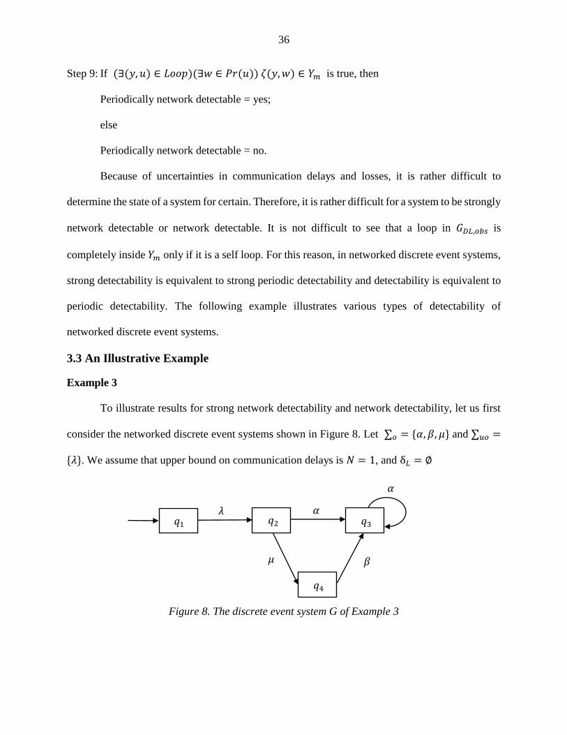
Because of uncertainties in communication delays and losses, it is rather difficult to

determine the state of a system for certain. Therefore, it is rather difficult for a system to be strongly

network detectable or network detectable. It is not difficult to see that a loop in 𝐺𝐷𝐿,𝑜𝑏𝑠 is

completely inside 𝑌𝑚 only if it is a self loop. For this reason, in networked discrete event systems,

strong detectability is equivalent to strong periodic detectability and detectability is equivalent to

periodic detectability. The following example illustrates various types of detectability of

networked discrete event systems.

3.3 An Illustrative Example

Example 3

To illustrate results for strong network detectability and network detectability, let us first

consider the networked discrete event systems shown in Figure 8. Let ∑𝑜 = {𝛼, 𝛽, 𝜇} and ∑𝑢𝑜 =

{𝜆}. We assume that upper bound on communication delays is 𝑁 = 1, and δ𝐿 = ∅

Figure 8. The discrete event system G of Example 3

𝑞1 𝑞2 𝑞3

𝑞4

𝜆 𝛼

𝛼

𝛽 𝜇

37

We construct 𝐺𝐿, observer 𝐺𝐿,𝑜𝑏𝑠, and the networked observer d 𝐺𝐷𝐿,𝑜𝑏𝑠 as in Figure 9, 10,

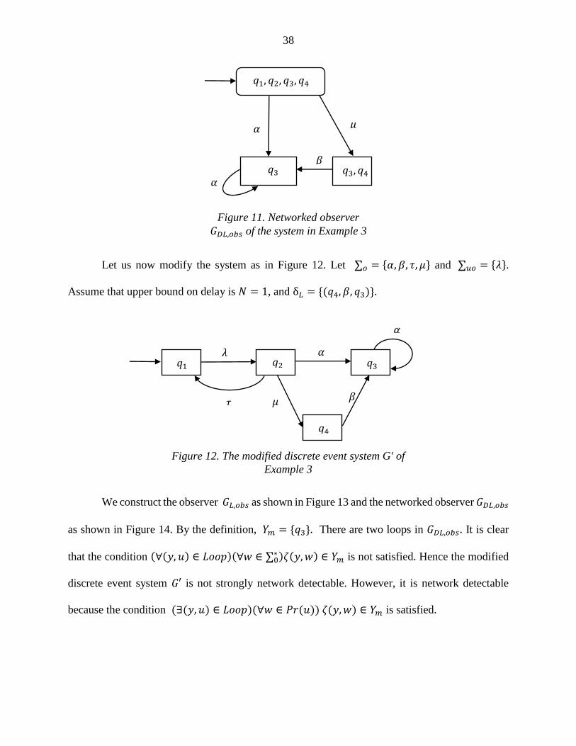
and 11 respectively. By definition, 𝑌𝑚 = {𝑞3}. There is only one loop in Figure 10. Clearly,

condition (∀(𝑦, 𝑢) ∈ 𝐿𝑜𝑜𝑝)(∀𝑤 ∈ ∑0∗ )휁(𝑦, 𝑤) ∈ 𝑌𝑚 is satisfied. Therefore, the system 𝐺 shown

in Figure 8 is strongly network detectable and hence also strong periodic network detectable.

Figure 10. Observer 𝐺𝐿,𝑜𝑏𝑠 of the

system in Example 3

𝑞1 𝑞2 𝑞3

𝑞4

𝛼

𝛼

𝛽 𝜇

휀

Figure 9. 𝐺𝐿 = 𝐿𝑂𝑆𝑆(𝐺) of Example 3.

𝑞1, 𝑞2

𝑞4 𝑞3

𝜇

𝛽

𝛼

𝛼

38

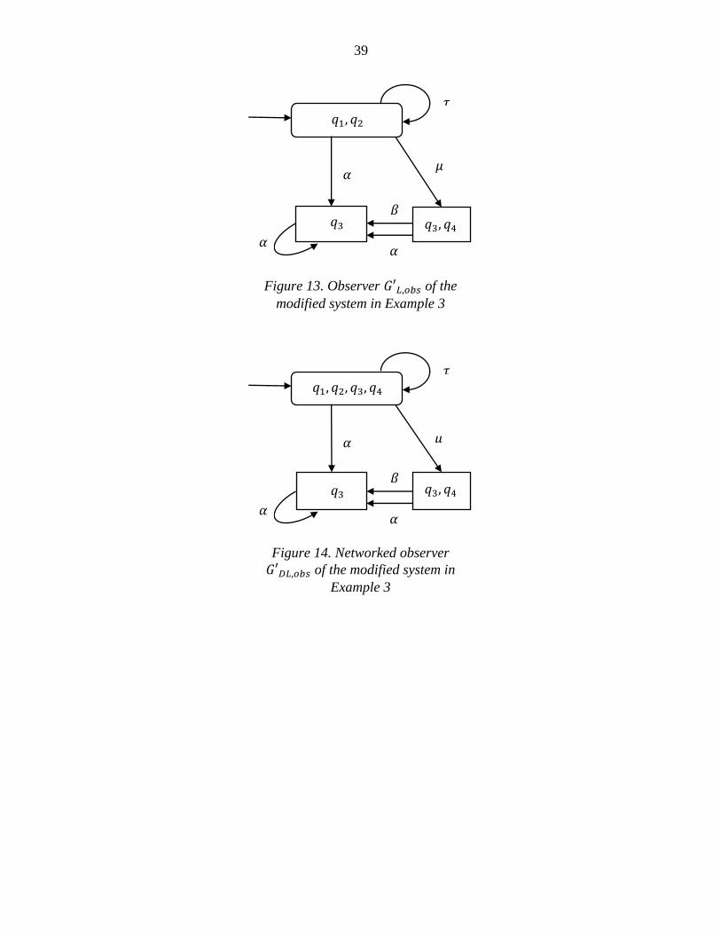
Let us now modify the system as in Figure 12. Let ∑𝑜 = {𝛼, 𝛽, 𝜏, 𝜇} and ∑𝑢𝑜 = {𝜆}.

Assume that upper bound on delay is 𝑁 = 1, and δ𝐿 = {(𝑞4, 𝛽, 𝑞3)}.

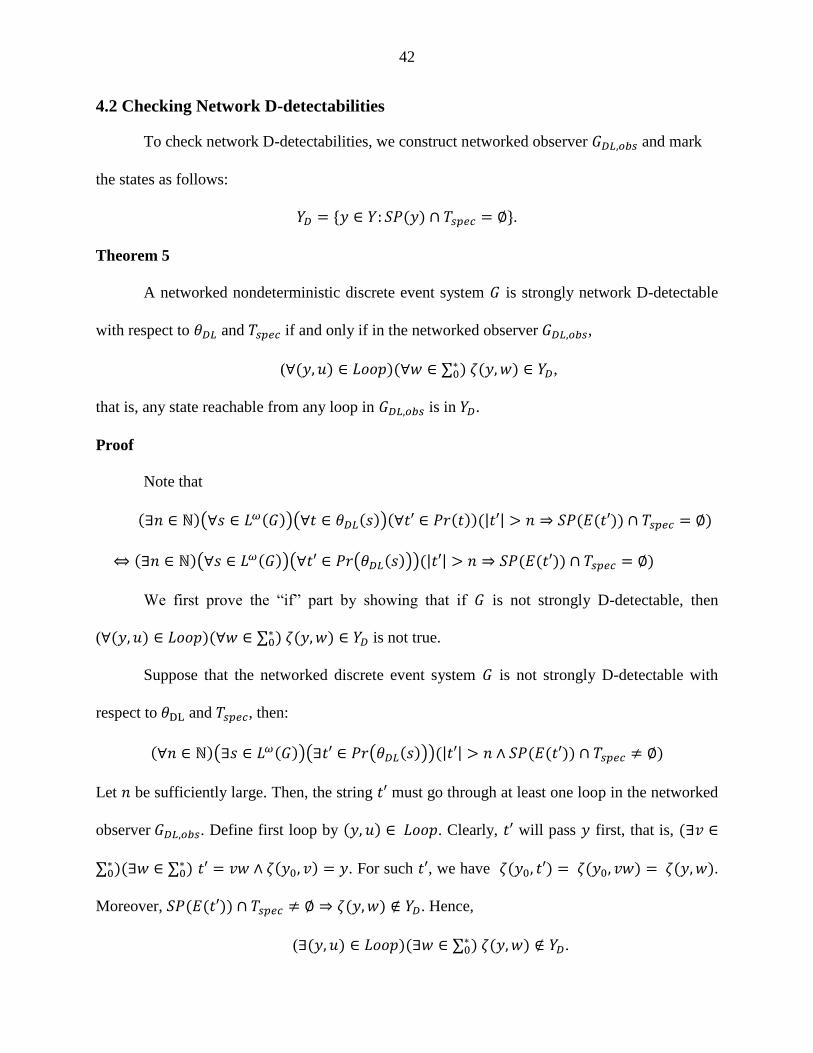
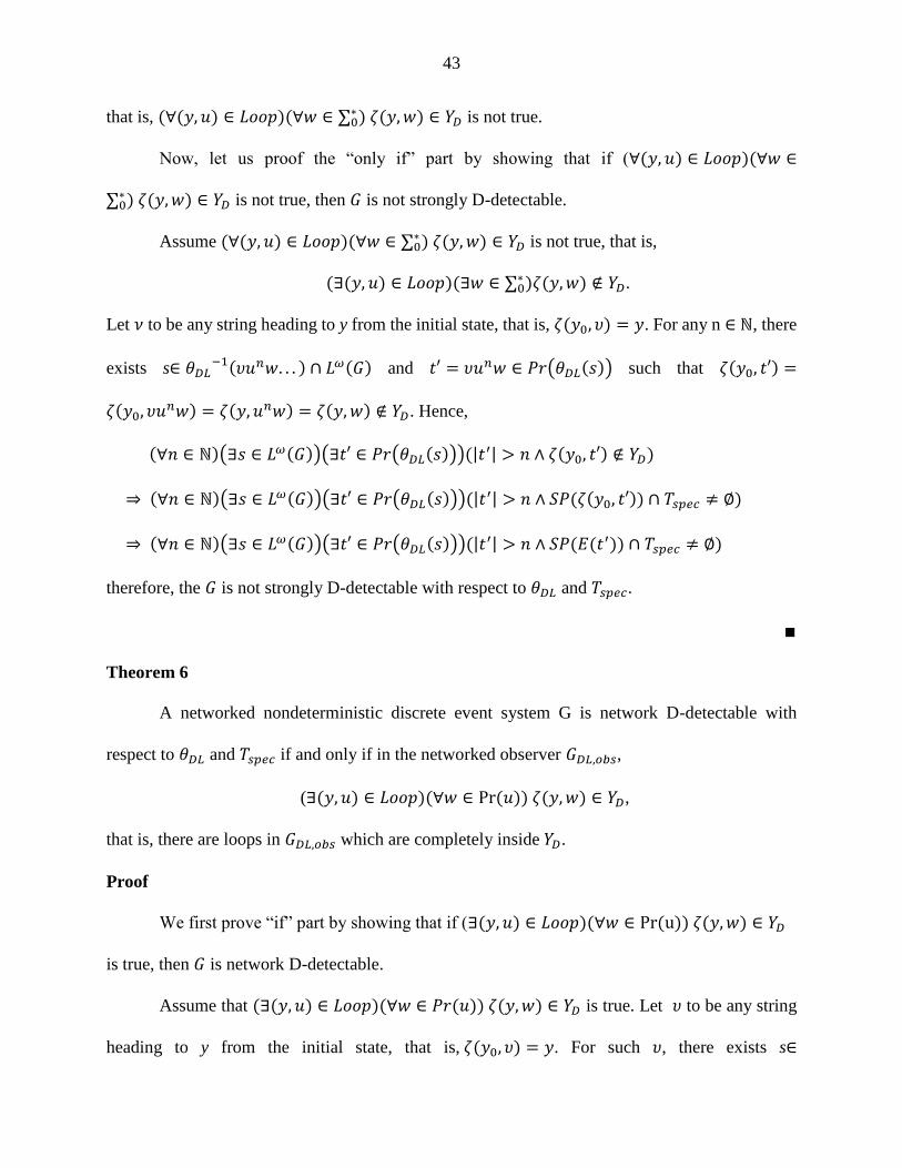
We construct the observer 𝐺𝐿,𝑜𝑏𝑠 as shown in Figure 13 and the networked observer 𝐺𝐷𝐿,𝑜𝑏𝑠

as shown in Figure 14. By the definition, 𝑌𝑚 = {𝑞3}. There are two loops in 𝐺𝐷𝐿,𝑜𝑏𝑠. It is clear

that the condition (∀(𝑦, 𝑢) ∈ 𝐿𝑜𝑜𝑝)(∀𝑤 ∈ ∑0∗ )휁(𝑦, 𝑤) ∈ 𝑌𝑚 is not satisfied. Hence the modified

discrete event system 𝐺′ is not strongly network detectable. However, it is network detectable

because the condition (∃(𝑦, 𝑢) ∈ 𝐿𝑜𝑜𝑝)(∀𝑤 ∈ 𝑃𝑟 (𝑢)) 휁(𝑦, 𝑤) ∈ 𝑌𝑚 is satisfied.


𝐺𝐷𝐿,𝑜𝑏𝑠 of the system in Example 3

Figure 12. The modified discrete event system G' of

Example 3

𝑞1, 𝑞2, 𝑞3, 𝑞4

𝑞3, 𝑞4 𝑞3

𝜇

𝛽

𝛼

𝛼

𝑞1 𝑞2 𝑞3

𝑞4

𝜆 𝛼

𝛼

𝛽 𝜇 𝜏

39

𝑞1, 𝑞2

𝑞3, 𝑞4 𝑞3

𝜇

𝛽

𝛼

𝛼

𝜏

𝛼

Figure 13. Observer 𝐺′𝐿,𝑜𝑏𝑠 of the

modified system in Example 3

𝑞1, 𝑞2, 𝑞3, 𝑞4

𝑞3, 𝑞4 𝑞3

𝜇

𝛽

𝛼

𝛼

𝜏

𝛼


𝐺′𝐷𝐿,𝑜𝑏𝑠 of the modified system in

Example 3

40

CHAPTER 4 D-DETECTABILITY OF NETWORKED DISCRETE EVENT

SYSTEMS

Due to uncertainty in communication delays and losses, it is hard to identify the state of a

networked discrete event system exactly. Hence, it is more likely that we will use network D-

detectability in practice. Network D-detectability can be defined as the ability to distinguish certain

pairs of states instead of identifying the current state. To this end, we define the set of all state

pairs as

𝑇 = {(𝑞, 𝑞′): 𝑞 ∈ 𝑄 ∧ 𝑞′ ∈ 𝑄}.

We specify the set of state pairs to be distinguished as a subset of 𝑇, that is,

𝑇𝑠𝑝𝑒𝑐 ⊆ 𝑇.

𝑇𝑠𝑝𝑒𝑐 is called a specification. The requirement of network D-detectability is that any state pair in

the specification 𝑇𝑠𝑝𝑒𝑐 needs to be distinguished after a finite number of observations. D-

detectability can be used to define stability [105-107] of discrete event systems by choosing

𝑇𝑠𝑝𝑒𝑐 = (𝑄 − 𝑄𝑠)×𝑄, where 𝑄𝑠 is the set of stable states [19].

If the state estimate is a subset 𝑄′ ⊆ 𝑄 , the set of indistinguishable state pairs is defined

as:

𝑆𝑃(𝑄′) = {(𝑞, 𝑞′): 𝑞 ∈ 𝑄′ ∧ 𝑞′ ∈ 𝑄′}𝑐 .

The set of indistinguishable state pairs after observing 𝑠 ∈ ∑∗ is given by:

𝑆𝑃(𝐸(휃𝐷𝐿(𝑠))) = {(𝑞, 𝑞′): 𝑞 ∈ 𝐸(휃𝐷𝐿(𝑠)) ∧ 𝑞′ ∈ 𝐸(휃𝐷𝐿(𝑠))}.

The following are the definitions of network D-detectabilities in terms of 𝑇𝑠𝑝𝑒𝑐 and

𝑆𝑃(𝐸(휃𝐷𝐿(𝑠))).

4.1 Definitions of Networked D-detectabilities.

We now define network D-detectabilities as follows.

41

Definition 5 (Strong Network D-detectability)

A networked nondeterministic discrete event system 𝐺 is said to be strongly network D-

detectable with respect to 휃𝐷𝐿 and 𝑇𝑠𝑝𝑒𝑐 if all state pairs in 𝑇𝑠𝑝𝑒𝑐 are distinguishable all the time,

after a finite number of observations, for all trajectories of the system. Formally,

(∃𝑛 ∈ ℕ)(∀𝑠 ∈ 𝐿𝜔(𝐺))(∀𝑡 ∈ 휃𝐷𝐿(𝑠))(∀𝑡′ ∈ 𝑃𝑟(𝑡))(|𝑡′| > 𝑛 ⇒ 𝑆𝑃(𝐸(𝑡′)) ∩ 𝑇𝑠𝑝𝑒𝑐 = ∅).

Definition 6 (Network D-detectability)

A networked nondeterministic discrete event system 𝐺 is said to be network D-detectable

with respect to 휃𝐷𝐿 and 𝑇𝑠𝑝𝑒𝑐 if all state pairs in 𝑇𝑠𝑝𝑒𝑐 are distinguishable all the time, after a finite

number of observations, for some trajectories of the system. Formally,

(∃𝑛 ∈ ℕ)(∃𝑠 ∈ 𝐿𝜔(𝐺))(∃𝑡 ∈ 휃𝐷𝐿(𝑠))(∀𝑡′ ∈ 𝑃𝑟(𝑡))(|𝑡′| > 𝑛 ⇒ 𝑆𝑃(𝐸(𝑡′)) ∩ 𝑇𝑠𝑝𝑒𝑐 = ∅).

Definition 7 (Strong Periodic Network D-Detectability)

A networked nondeterministic discrete event system 𝐺 is said to be strongly periodically

network D-detectable with respect to 휃𝐷𝐿 and 𝑇𝑠𝑝𝑒𝑐 if all state pairs in 𝑇𝑠𝑝𝑒𝑐 are periodically

distinguishable for all trajectories of the system. Formally,


(𝑡′𝑡′′ ∈ 𝑃𝑟(𝑡) ∧ |𝑡′′| < 𝑛 ∧ 𝑆𝑃(𝐸(𝑡′𝑡′′)) ∩ 𝑇𝑠𝑝𝑒𝑐 = ∅).

Definition 8 (Periodic Network D-Detectability)

A networked nondeterministic discrete event system 𝐺 is said to be periodically network

D-detectable with respect to 휃𝐷𝐿 and 𝑇𝑠𝑝𝑒𝑐 if all state pairs in 𝑇𝑠𝑝𝑒𝑐 are periodically distinguishable

for some trajectories of the system. That is,



42

4.2 Checking Network D-detectabilities

To check network D-detectabilities, we construct networked observer 𝐺𝐷𝐿,𝑜𝑏𝑠 and mark

the states as follows:

𝑌𝐷 = {𝑦 ∈ 𝑌: 𝑆𝑃(𝑦) ∩ 𝑇𝑠𝑝𝑒𝑐 = ∅}.

Theorem 5

A networked nondeterministic discrete event system 𝐺 is strongly network D-detectable

with respect to 휃𝐷𝐿 and 𝑇𝑠𝑝𝑒𝑐 if and only if in the networked observer 𝐺𝐷𝐿,𝑜𝑏𝑠,

(∀(𝑦, 𝑢) ∈ 𝐿𝑜𝑜𝑝)(∀𝑤 ∈ ∑0∗ ) 휁(𝑦, 𝑤) ∈ 𝑌𝐷,

that is, any state reachable from any loop in 𝐺𝐷𝐿,𝑜𝑏𝑠 is in 𝑌𝐷.

Proof

Note that

(∃𝑛 ∈ ℕ)(∀𝑠 ∈ 𝐿𝜔(𝐺))(∀𝑡 ∈ 휃𝐷𝐿(𝑠))(∀𝑡′ ∈ 𝑃𝑟(𝑡))(|𝑡′| > 𝑛 ⇒ 𝑆𝑃(𝐸(𝑡′)) ∩ 𝑇𝑠𝑝𝑒𝑐 = ∅)

⇔ (∃𝑛 ∈ ℕ)(∀𝑠 ∈ 𝐿𝜔(𝐺))(∀𝑡′ ∈ 𝑃𝑟(휃𝐷𝐿(𝑠)))(|𝑡′| > 𝑛 ⇒ 𝑆𝑃(𝐸(𝑡′)) ∩ 𝑇𝑠𝑝𝑒𝑐 = ∅)

We first prove the “if” part by showing that if 𝐺 is not strongly D-detectable, then

(∀(𝑦, 𝑢) ∈ 𝐿𝑜𝑜𝑝)(∀𝑤 ∈ ∑0∗ ) 휁(𝑦, 𝑤) ∈ 𝑌𝐷 is not true.

Suppose that the networked discrete event system 𝐺 is not strongly D-detectable with

respect to 휃DL and 𝑇𝑠𝑝𝑒𝑐, then:

(∀𝑛 ∈ ℕ)(∃𝑠 ∈ 𝐿𝜔(𝐺))(∃𝑡′ ∈ 𝑃𝑟(휃𝐷𝐿(𝑠)))(|𝑡′| > 𝑛 ∧ 𝑆𝑃(𝐸(𝑡′)) ∩ 𝑇𝑠𝑝𝑒𝑐 ≠ ∅)

Let 𝑛 be sufficiently large. Then, the string 𝑡′ must go through at least one loop in the networked

observer 𝐺𝐷𝐿,𝑜𝑏𝑠. Define first loop by (𝑦, 𝑢) ∈ 𝐿𝑜𝑜𝑝. Clearly, 𝑡′ will pass 𝑦 first, that is, (∃𝑣 ∈

∑0∗ )(∃𝑤 ∈ ∑0

∗ ) 𝑡′ = 𝑣𝑤 ∧ 휁(𝑦0, 𝑣) = 𝑦. For such 𝑡′, we have 휁(𝑦0, 𝑡′) = 휁(𝑦0, 𝑣𝑤) = 휁(𝑦, 𝑤).

Moreover, 𝑆𝑃(𝐸(𝑡′)) ∩ 𝑇𝑠𝑝𝑒𝑐 ≠ ∅ ⇒ 휁(𝑦, 𝑤) ∉ 𝑌𝐷. Hence,

(∃(𝑦, 𝑢) ∈ 𝐿𝑜𝑜𝑝)(∃𝑤 ∈ ∑0∗ ) 휁(𝑦, 𝑤) ∉ 𝑌𝐷.

43

that is, (∀(𝑦, 𝑢) ∈ 𝐿𝑜𝑜𝑝)(∀𝑤 ∈ ∑0∗ ) 휁(𝑦, 𝑤) ∈ 𝑌𝐷 is not true.

Now, let us proof the “only if” part by showing that if (∀(𝑦, 𝑢) ∈ 𝐿𝑜𝑜𝑝)(∀𝑤 ∈

∑0∗ ) 휁(𝑦, 𝑤) ∈ 𝑌𝐷 is not true, then 𝐺 is not strongly D-detectable.

Assume (∀(𝑦, 𝑢) ∈ 𝐿𝑜𝑜𝑝)(∀𝑤 ∈ ∑0∗ ) 휁(𝑦, 𝑤) ∈ 𝑌𝐷 is not true, that is,

(∃(𝑦, 𝑢) ∈ 𝐿𝑜𝑜𝑝)(∃𝑤 ∈ ∑0∗ )휁(𝑦, 𝑤) ∉ 𝑌𝐷.

Let 𝜈 to be any string heading to y from the initial state, that is, 휁(𝑦0, 𝜐) = 𝑦. For any n ∈ ℕ, there

exists s∈ 휃𝐷𝐿−1(𝜐𝑢𝑛𝑤. . . ) ∩ 𝐿𝜔(𝐺) and 𝑡′ = 𝜐𝑢𝑛𝑤 ∈ 𝑃𝑟(휃𝐷𝐿(𝑠)) such that 휁(𝑦0, 𝑡′) =

휁(𝑦0, 𝜐𝑢𝑛𝑤) = 휁(𝑦, 𝑢𝑛𝑤) = 휁(𝑦, 𝑤) ∉ 𝑌𝐷. Hence,

(∀𝑛 ∈ ℕ)(∃𝑠 ∈ 𝐿𝜔(𝐺))(∃𝑡′ ∈ 𝑃𝑟(휃𝐷𝐿(𝑠)))(|𝑡′| > 𝑛 ∧ 휁(𝑦0, 𝑡′) ∉ 𝑌𝐷)

⇒ (∀𝑛 ∈ ℕ)(∃𝑠 ∈ 𝐿𝜔(𝐺))(∃𝑡′ ∈ 𝑃𝑟(휃𝐷𝐿(𝑠)))(|𝑡′| > 𝑛 ∧ 𝑆𝑃(휁(𝑦0, 𝑡′)) ∩ 𝑇𝑠𝑝𝑒𝑐 ≠ ∅)

⇒ (∀𝑛 ∈ ℕ)(∃𝑠 ∈ 𝐿𝜔(𝐺))(∃𝑡′ ∈ 𝑃𝑟(휃𝐷𝐿(𝑠)))(|𝑡′| > 𝑛 ∧ 𝑆𝑃(𝐸(𝑡′)) ∩ 𝑇𝑠𝑝𝑒𝑐 ≠ ∅)

therefore, the 𝐺 is not strongly D-detectable with respect to 휃𝐷𝐿 and 𝑇𝑠𝑝𝑒𝑐.

∎

Theorem 6

A networked nondeterministic discrete event system G is network D-detectable with

respect to 휃𝐷𝐿 and 𝑇𝑠𝑝𝑒𝑐 if and only if in the networked observer 𝐺𝐷𝐿,𝑜𝑏𝑠,

(∃(𝑦, 𝑢) ∈ 𝐿𝑜𝑜𝑝)(∀𝑤 ∈ Pr (𝑢)) 휁(𝑦, 𝑤) ∈ 𝑌𝐷,

that is, there are loops in 𝐺𝐷𝐿,𝑜𝑏𝑠 which are completely inside 𝑌𝐷.

Proof

We first prove “if” part by showing that if (∃(𝑦, 𝑢) ∈ 𝐿𝑜𝑜𝑝)(∀𝑤 ∈ Pr (u)) 휁(𝑦, 𝑤) ∈ 𝑌𝐷

is true, then 𝐺 is network D-detectable.

Assume that (∃(𝑦, 𝑢) ∈ 𝐿𝑜𝑜𝑝)(∀𝑤 ∈ 𝑃𝑟 (𝑢)) 휁(𝑦, 𝑤) ∈ 𝑌𝐷 is true. Let 𝜐 to be any string

heading to y from the initial state, that is, 휁(𝑦0, 𝜐) = 𝑦. For such 𝜐, there exists s∈

44

휃𝐷𝐿−1(𝜐𝑢𝑢𝑢. . . ) ∩ 𝐿𝜔(𝐺), 𝑡 = 𝜐𝑢𝑢𝑢. . . ∈ 휃𝐷𝐿(𝑠), and 𝑛 = |𝜐| ∈ ℕ such that for all 𝑡′ ∈ 𝑃𝑟(𝑡),

|𝑡′| > 𝑛 ⇒ 𝑡′ = 𝜐𝑢𝑗𝑤, for some 𝑗 ∈ ℕ and 𝑤 ∈ 𝑃𝑟 (u). Hence, 휁(𝑦0, 𝑡′) = 휁(𝑦0, 𝜐𝑢𝑗𝑤) =

휁(𝑦, 𝑢𝑗𝑤) = 휁(𝑦, 𝑤) ∈ 𝑌𝐷. Therefore,

(∃𝑛 ∈ ℕ)(∃𝑠 ∈ 𝐿𝜔(𝐺))(∃𝑡 ∈ 휃𝐷𝐿(𝑠))(∀𝑡′ ∈ 𝑃𝑟(𝑡))(|𝑡′| > 𝑛 ⇒ 휁(𝑦, 𝑤) ∈ 𝑌𝐷)

⇒ (∃𝑛 ∈ ℕ)(∃𝑠 ∈ 𝐿𝜔(𝐺))(∃𝑡 ∈ 휃𝐷𝐿(𝑠))(∀𝑡′ ∈ 𝑃𝑟(𝑡))(|𝑡′| > 𝑛 ⇒ 𝑆𝑃(휁(𝑦, 𝑤)) ∩ 𝑇𝑠𝑝𝑒𝑐 = ∅)

⇒ (∃𝑛 ∈ ℕ)(∃𝑠 ∈ 𝐿𝜔(𝐺))(∃𝑡 ∈ 휃𝐷𝐿(𝑠))(∀𝑡′ ∈ 𝑃𝑟(𝑡))(|𝑡′| > 𝑛 ⇒ 𝑆𝑃(𝐸(𝑡′)) ∩ 𝑇𝑠𝑝𝑒𝑐 = ∅)

Hence, 𝐺 is network D-detectable with respect to 휃𝐷𝐿.

We next prove the “only if” part by showing if 𝐺 is D-detectable with respect to 휃𝐷𝐿, then

(∃(𝑦, 𝑢) ∈ 𝐿𝑜𝑜𝑝)(∀𝑤 ∈ 𝑃𝑟 (u)) 휁(𝑦, 𝑤) ∈ 𝑌𝐷 is true.

Suppose that 𝐺 is D-detectable with respect to 휃𝐷𝐿, that is,

(∃𝑛 ∈ ℕ)(∃𝑠 ∈ 𝐿𝜔(𝐺))(∃𝑡 ∈ 휃𝐷𝐿(𝑠))(∀𝑡′ ∈ 𝑃𝑟(𝑡))(|𝑡′| > 𝑛 ⇒ 𝑆𝑃(𝐸(𝑡′)) ∩ 𝑇𝑠𝑝𝑒𝑐 = ∅)

Then such 𝑡 must go through at least one loop in 𝐺𝐷𝐿,𝑜𝑏𝑠. Denote a loop after 𝑛 transitions

by (𝑦, 𝑢) ∈ 𝐿𝑜𝑜𝑝. Let 𝜐 to the prefix of 𝑡 that leads to 𝑦, that is, 휁(𝑦0, 𝜐) = 𝑦. Since 𝑆𝑃(𝐸(𝑡′)) ∩

𝑇𝑠𝑝𝑒𝑐 = ∅ ⇒ 𝑆𝑃(휁(𝑦0, 𝑡′)) ∩ 𝑇𝑠𝑝𝑒𝑐 = ∅ ⇒ 휁(𝑦0, 𝑡′) ∈ 𝑌𝐷, all states in the loop are in 𝑌𝐷. In other

words,

(∃(𝑦, 𝑢) ∈ 𝐿𝑜𝑜𝑝)(∀𝑤 ∈ Pr (u)) 휁(𝒴, 𝑤) ∈ 𝑌𝐷 is true.

∎

Theorem 7

A networked nondeterministic discrete event system 𝐺 is strongly periodically network D-

detectable with respect to 휃𝐷𝐿 and 𝑇𝑠𝑝𝑒𝑐 if and only if in the networked observer 𝐺𝐷𝐿,𝑜𝑏𝑠,

(∀(𝑦, 𝑢) ∈ 𝐿𝑜𝑜𝑝)(∃𝑤 ∈ Pr (𝑢)) 휁(𝑦, 𝑤) ∈ 𝑌𝐷,

that is, every loop in 𝐺𝐷𝐿,𝑜𝑏𝑠 must contain at least one state belonging to 𝑌𝐷.

45

Proof

We first need to prove the “if” part by showing that if G is not strongly periodically D-

detectable, then (∀(𝑦, 𝑢) ∈ 𝐿𝑜𝑜𝑝)(∃𝑤 ∈ 𝑃𝑟 (u)) 휁(𝑦, 𝑤) ∈ 𝑌𝐷 is not true.

Suppose that the networked discrete event system G is not strongly periodically network

D-detectable with respect to 휃DL and 𝑇𝑠𝑝𝑒𝑐, then,


(𝑡′𝑡′′ ∈ 𝑃𝑟(𝑡) ∧ |𝑡′′| < 𝑛 ⇒ 𝑆𝑃(𝐸(𝑡′𝑡′′)) ∩ 𝑇𝑠𝑝𝑒𝑐 ≠ ∅).

Take 𝑛 = |𝑌| + 1. By the above equation,

(∃𝑠 ∈ 𝐿𝜔(𝐺))(∃𝑡 ∈ 휃𝐷𝐿(𝑠))(∃𝑡′ ∈ 𝑃𝑟(𝑡))(∀𝑡′′ ∈ 𝛴𝑜∗)

(𝑡′𝑡′′ ∈ 𝑃𝑟(𝑡) ∧ |𝑡′′| < |𝑌| + 1 ⇒ 𝑆𝑃(𝐸(𝑡′𝑡′′)) ∩ 𝑇𝑠𝑝𝑒𝑐 ≠ ∅).

Consider the next 𝑛 = |𝑌| + 1 states after 𝑡′ in 𝐺𝐷𝐿,𝑜𝑏𝑠 on the path of 𝑡′′, since 𝑆𝑃(𝐸(𝑡′𝑡′′)) ∩

𝑇𝑠𝑝𝑒𝑐 ≠ ∅, all these states do not belong to 𝑌𝐷. Since the path of 𝑡′′ is greater than |𝑌|, it must

contain a loop. Denote this loop by (𝑦, 𝑢) ∈ 𝐿𝑜𝑜𝑝. Since all states visited by (𝑦, 𝑢) do not belong

to 𝑌𝐷,

(∃(𝑦, 𝑢) ∈ 𝐿𝑜𝑜𝑝)(∀𝑤 ∈ 𝑃𝑟 (u)) 휁(𝑦, 𝑤) ∉ 𝑌𝐷.

That is,

(∀(𝑦, 𝑢) ∈ 𝐿𝑜𝑜𝑝)(∃𝑤 ∈ 𝑃𝑟 (u)) 휁(𝑦, 𝑤) ∈ 𝑌𝐷

is not true.

Next, we prove the “only if” part by showing that if (∀(𝑦, 𝑢) ∈ 𝐿𝑜𝑜𝑝)(∃𝑤 ∈

𝑃𝑟 (u)) 휁(𝑦, 𝑤) ∈ 𝑌𝐷 is not true, then 𝐺 is not strongly periodically network D-detectable.

Suppose that (∀(𝑦, 𝑢) ∈ 𝐿𝑜𝑜𝑝)(∃𝑤 ∈ 𝑃𝑟 (u)) 휁(𝑦, 𝑤) ∈ 𝑌𝐷 is not true, that is,

(∃(𝑦, 𝑢) ∈ 𝐿𝑜𝑜𝑝)(∀𝑤 ∈ 𝑃𝑟 (u)) 휁(𝑦, 𝑤) ∉ 𝑌𝐷 .

46

Let 𝜐 to be any string heading to y from the initial state, that is, 휁(𝑦0, 𝜐) = 𝑦. In this case, for all

𝑛 ∈ ℕ, there exists s∈ 휃𝐷𝐿−1(𝜐𝑢𝑢𝑢. . . ) ∩ 𝐿𝜔(𝐺), 𝑡 = 𝜐𝑢𝑢𝑢 … ∈ 휃𝐷𝐿(𝑠) , and 𝑡′ = 𝜐 such that we

can let 𝑡′′ to travel the loop (𝑦, 𝑢) sufficient number of times so that the following is true


(𝑡′𝑡′′ ∈ 𝑃𝑟(𝑡) ∧ |𝑡′′| < 𝑛 ⇒ 휁(𝑦0, 𝑡′𝑡′′) = 휁(𝑦, 𝑡′′) ∉ 𝑌𝐷)

Which implies


(𝑡′𝑡′′ ∈ 𝑃𝑟(𝑡) ∧ |𝑡′′| < 𝑛 ⇒ 𝑆𝑃(𝐸(𝑡′𝑡′′)) ∩ 𝑇𝑠𝑝𝑒𝑐 ≠ ∅).

In other words, 𝐺 is not strongly periodically network D-detectable with respect to 휃𝐷𝐿 and

𝑇𝑠𝑝𝑒𝑐.

∎

Theorem 8

A networked nondeterministic discrete event system 𝐺 is periodically network D-

detectable with respect to 휃𝐷𝐿 and 𝑇𝑠𝑝𝑒𝑐 if and only if in the networked observer 𝐺𝐷𝐿,𝑜𝑏𝑠,

(∃(𝑦, 𝑢) ∈ 𝐿𝑜𝑜𝑝)(∃𝑤 ∈ Pr (𝑢)) 휁(𝑦, 𝑤) ∈ 𝑌𝐷,

that is, there are loops in 𝐺𝐷𝐿,𝑜𝑏𝑠 that include no less than one state belonging to 𝑌𝐷.

Proof

We first prove “only if” part. Suppose that 𝐺 is periodically D-detectable with reference to

휃𝐷𝐿 and 𝑇𝑠𝑝𝑒𝑐, that is,



47

Then 𝑡 must go through a loop in 𝐺𝐷𝐿,𝑜𝑏𝑠 in which 𝑆𝑃(𝐸(𝑡′𝑡′′)) ∩ 𝑇𝑠𝑝𝑒𝑐 = ∅ is true for

some 𝑡′′. Designate this loop by (𝑦, 𝑢) ∈ 𝐿𝑜𝑜𝑝, then

(∃𝑡′′ ∈ 𝛴𝑜∗)𝑆𝑃(𝐸(𝑡′𝑡′′)) ∩ 𝑇𝑠𝑝𝑒𝑐 = ∅ ⇒ (∃𝑤 ∈ 𝑃𝑟 (u)) 휁(𝑦, 𝑤) ∈ 𝑌𝐷.

Therefore, (∃(𝑦, 𝑢) ∈ 𝐿𝑜𝑜𝑝)(∃𝑤 ∈ 𝑃𝑟 (u)) 휁(𝑦, 𝑤) ∈ 𝑌𝐷.

We next prove the “if” part. Suppose that (∃(𝑦, 𝑢) ∈ 𝐿𝑜𝑜𝑝)(∃𝑤 ∈ 𝑃𝑟 (u)) 휁(𝑦, 𝑤) ∈ 𝑌𝐷 is

true. Let 𝜐 to be any string heading to y from the initial state, that is, 휁(𝑦0, 𝜐) = 𝑦. In this case,

there exists 𝑛 = |𝜐𝑢| ∈ ℕ, 𝑠 ∈ 휃𝐷𝐿−1(𝜐𝑢𝑢𝑢. . . ) ∩ 𝐿𝜔(𝐺), and 𝑡 = 𝜐𝑢𝑢𝑢 … ∈ 휃𝐷𝐿(𝑠) such that


(𝑡′𝑡′′ ∈ 𝑃𝑟(𝑡) ∧ |𝑡′′| < 𝑛 ∧ 휁(𝑦0, 𝑡′𝑡′′) ∈ 𝑌𝐷),

where 𝑡′𝑡′′ = 𝜐𝑢𝑗𝑤 for some j ∈ ℕ. Therefore,



In other words, 𝐺 is periodically network D-detectable with respect to 휃𝐷𝐿 and 𝑇𝑠𝑝𝑒𝑐.

∎

4.3 An Algorithm to Check Network D-detectabilities of Discrete Event Systems

In summary, we can check network D-detectabilities using the following algorithm.

Algorithm 2



A specification 𝑇𝑠𝑝𝑒𝑐 ⊆ 𝑇.

Output: Network D-detectable (= yes or no)

Strongly network D-detectable (= yes or no)

Periodically network D-detectable (= yes or no)

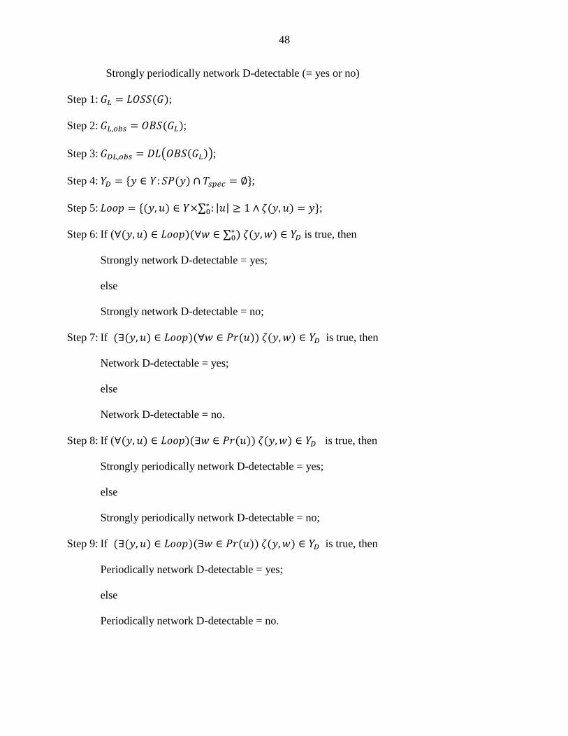
48

Strongly periodically network D-detectable (= yes or no)

Step 1: 𝐺𝐿 = 𝐿𝑂𝑆𝑆(𝐺);

Step 2: 𝐺𝐿,𝑜𝑏𝑠 = 𝑂𝐵𝑆(𝐺𝐿);

Step 3: 𝐺𝐷𝐿,𝑜𝑏𝑠 = 𝐷𝐿(𝑂𝐵𝑆(𝐺𝐿));

Step 4: 𝑌𝐷 = {𝑦 ∈ 𝑌: 𝑆𝑃(𝑦) ∩ 𝑇𝑠𝑝𝑒𝑐 = ∅};

Step 5: 𝐿𝑜𝑜𝑝 = {(𝑦, 𝑢) ∈ 𝑌×∑0∗ : |𝑢| ≥ 1 ∧ 휁(𝑦, 𝑢) = 𝑦};

Step 6: If (∀(𝑦, 𝑢) ∈ 𝐿𝑜𝑜𝑝)(∀𝑤 ∈ ∑0∗ ) 휁(𝑦, 𝑤) ∈ 𝑌𝐷 is true, then

Strongly network D-detectable = yes;

else

Strongly network D-detectable = no;

Step 7: If (∃(𝑦, 𝑢) ∈ 𝐿𝑜𝑜𝑝)(∀𝑤 ∈ 𝑃𝑟 (𝑢)) 휁(𝑦, 𝑤) ∈ 𝑌𝐷 is true, then

Network D-detectable = yes;

else

Network D-detectable = no.

Step 8: If (∀(𝑦, 𝑢) ∈ 𝐿𝑜𝑜𝑝)(∃𝑤 ∈ 𝑃𝑟 (𝑢)) 휁(𝑦, 𝑤) ∈ 𝑌𝐷 is true, then

Strongly periodically network D-detectable = yes;

else

Strongly periodically network D-detectable = no;

Step 9: If (∃(𝑦, 𝑢) ∈ 𝐿𝑜𝑜𝑝)(∃𝑤 ∈ 𝑃𝑟 (𝑢)) 휁(𝑦, 𝑤) ∈ 𝑌𝐷 is true, then

Periodically network D-detectable = yes;

else

Periodically network D-detectable = no.

49

4.4 Illustrative Examples

Example 4

Let us consider the discrete event system shown in Figure 15. The system represents a

nuclear reactor with six states, and each state represents the speed of nuclear reaction from very

slow (𝑞1) to very high (𝑞6). The transition from state to state requires an event 𝛼 or 𝛽 to happen.

Physically, α and β represent the removing and inserting of the control rods of the reactor to a

known position. Assume that ∑𝑜 = {𝛼1, 𝛼2, 𝛼4, 𝛼5, 𝛽1, 𝛽2, 𝛽4, 𝛽5, 𝛽6} and ∑𝑢𝑜 = {𝛼3, 𝛽3} because

of sensor failure. Also, assume that upper bound on communication delays is 𝑁 = 1, and δ𝐿 =

{(𝑞3, 𝛽2, 𝑞2), (𝑞2, 𝛼2, 𝑞3)}. The specification is given by

𝑇𝑠𝑝𝑒𝑐 = {(𝑞1, 𝑞5), (𝑞1, 𝑞6), (𝑞2, 𝑞5), (𝑞2, 𝑞6)}

The specification above used to distinguish the safe states {𝑞1, 𝑞2} from the dangerous states

{𝑞5, 𝑞6}.

Figure 16. Automaton 𝐺𝐿 of the system in Example 4

Figure 15. A discrete event system G representing a nuclear

reactor

𝛼4 𝛼3 𝛼2 𝛼1

𝛽5 𝛽4 𝛽3 𝛽2 𝛽1

𝑞1 𝑞2 𝑞3 𝑞4 𝑞5 𝑞6

𝛼5

𝛽6

휀

𝛼4 휀 𝛼2 𝛼1

𝛽5 𝛽4 휀 𝛽2 𝛽1

𝑞1 𝑞2 𝑞3 𝑞4 𝑞5 𝑞6

𝛼5

𝛽6

휀

50

Using Algorithm 2, we calculate 𝐺𝐿, 𝐺𝐿,𝑜𝑏𝑠, and networked observer 𝐺𝐷𝐿,𝑜𝑏𝑠 as shown in

Figures 16, 17, and 18 respectively.

The marked states are calculated as

𝑌𝐷 = {{𝑞1, 𝑞2}, {𝑞1, 𝑞2, 𝑞3, 𝑞4}, {𝑞4, 𝑞5, 𝑞6}, {𝑞4, 𝑞5, 𝑞6}}

By Algorithm 2, we conclude:

Strongly network D-detectable = no;

Network D-detectable = yes;

Strongly periodically network D-detectable = no;

Periodically network D-detectable = yes;

𝑞3, 𝑞4

𝛼4 𝛼2 𝛼1

𝛽5 𝛽4 𝛽2 𝛽1

𝑞1 𝑞2, 𝑞3, 𝑞4 𝑞5

5

𝑞6

𝛼5

𝛽6

𝛼4

Figure 17. Observer 𝐺𝐿,𝑜𝑏𝑠 of the system in Example 4

𝑞2, 𝑞3, 𝑞4, 𝑞5

𝛼4 𝛼2 𝛼1

𝛽5 𝛽4 𝛽2 𝛽1

𝑞1, 𝑞2 𝑞1, 𝑞2, 𝑞3, 𝑞4 𝑞4, 𝑞5, 𝑞6 𝑞4, 𝑞5, 𝑞6

𝛼5

𝛽6

𝛼4

Figure 18. Networked observer 𝐺𝐷𝐿,𝑜𝑏𝑠 of the system in Example 4

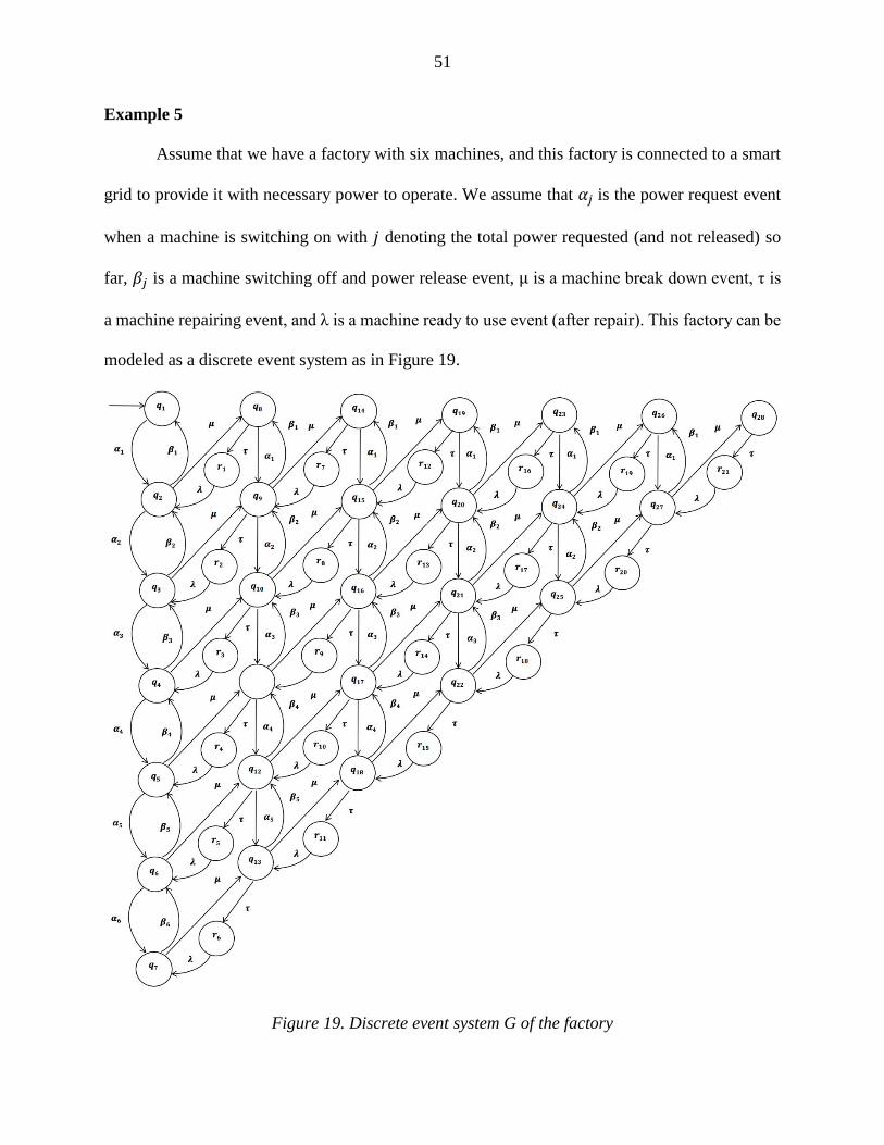
51

Example 5

Assume that we have a factory with six machines, and this factory is connected to a smart

grid to provide it with necessary power to operate. We assume that 𝛼𝑗 is the power request event

when a machine is switching on with 𝑗 denoting the total power requested (and not released) so

far, 𝛽𝑗 is a machine switching off and power release event, µ is a machine break down event, τ is

a machine repairing event, and λ is a machine ready to use event (after repair). This factory can be

modeled as a discrete event system as in Figure 19.

Figure 19. Discrete event system G of the factory

52

Each 𝑞𝑖 state represents a unique state of the system; for example, 𝑞1 represents the state

of the system where there are no machines working, and 𝑞5 represents the state of the system where

there are four machines working. Similarly, 𝑟𝑖 states are transient states where some machines have

just been repaired. For example, 𝑟8 is the state of the system where there are one machine working

and two being repaired.

Figure 20. Networked observer 𝐺𝐷𝐿,𝑜𝑏𝑠 , for the first few states, with 𝑁 = 1

53

We assume there is no loss in events, i.e., only the delay can affect the system. Also, assume

that the upper bound on observation delays 𝑁 = 1. We construct 𝐺𝐷𝐿,𝑜𝑏𝑠 observer as shown in

Figure 20. Note that we only show some states in 𝐺𝐷𝐿,𝑜𝑏𝑠 in order to make it easy to read.

To better schedule the power production, the power supplier would like to know how much

power the factory is consuming (which is roughly proportional to the number of machines

working). Hence, we group different sets of states as follows:

𝑄0 = {𝑞1, 𝑞8, 𝑞14, 𝑞19, 𝑞23, 𝑞26, 𝑞28, 𝑟1, 𝑟7, 𝑟12, 𝑟16, 𝑟19}; no machines is working.

𝑄1 = {𝑞2, 𝑞9, 𝑞15, 𝑞20, 𝑞24, 𝑞27, 𝑟2, 𝑟8, 𝑟13, 𝑟17, 𝑟20}; one machine is working.

𝑄2 = {𝑞3, 𝑞10, 𝑞16, 𝑞21, 𝑞25, 𝑟3, 𝑟9, 𝑟14, 𝑟18}; two machines are working.

𝑄3 = {𝑞4, 𝑞11, 𝑞17, 𝑞22, 𝑟4, 𝑟10, 𝑟15}; three Machines are working.

𝑄4 = {𝑞5, 𝑞12, 𝑞18, 𝑟5, 𝑟11}; four Machines are working.

𝑄5 = {𝑞6, 𝑞13, 𝑟6}; five machines are working.

𝑄6 = {𝑞7}; six machines are working.

Due to communications delays, the power supplier may not know the exact power

consumption of the factory. However, it would like at least to distinguish states in 𝑄𝑗 from state

in 𝑄𝑗+3. Hence, the specification is given by

𝑇𝑠𝑝𝑒𝑐={(𝑄0×𝑄3)∪ (𝑄0×𝑄4)∪ (𝑄0×𝑄5) ∪ (𝑄0×𝑄6) ∪ (𝑄1×𝑄4) ∪ (𝑄1×𝑄5) ∪ (𝑄1×𝑄6) ∪

(𝑄2×𝑄5) ∪ (𝑄2×𝑄6) ∪ (𝑄3×𝑄6)}

For 𝑁 = 1, we can successfully distinguish all the state pairs specified by 𝑇𝑠𝑝𝑒𝑐. Therefore,

the networked discrete event system is strongly network D-detectable. Is this still possible if 𝑁 =

2? Let us construct 𝐺𝐷𝐿,𝑜𝑏𝑠 for 𝑁 = 2 as in Figure 21. We notice that we can distinguish some but

not all the state pairs specified by 𝑇𝑠𝑝𝑒𝑐. Therefore, the discrete event system is only network D-

detectable.

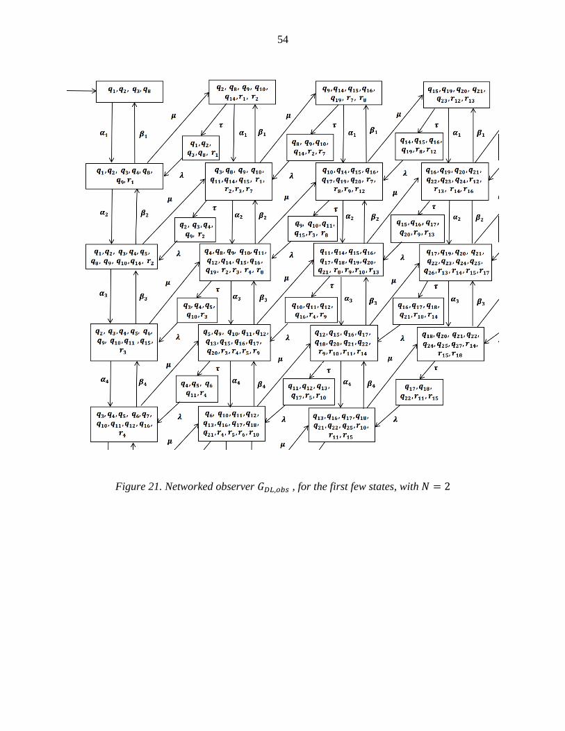
54

Figure 21. Networked observer 𝐺𝐷𝐿,𝑜𝑏𝑠 , for the first few states, with 𝑁 = 2

55

CHAPTER 5 PROPERTIES OF NETWORK DETECTABILITY

Intuitively, we see that if the upper bound on communication delays N increases, then there

are more uncertainties in the state estimate (that is, the state estimate is larger). Let us formally

prove this as follows. We use 𝐺𝐷𝐿,𝑜𝑏𝑠𝑁 to denote the network observer with observation delays

bounded by N. Note that communication losses are specified by transitions in 𝛿𝐿 and hence are

independent of N.

5.1 Properties

Lemma 1

For a networked discrete event system 𝐺, let

𝐺𝐷𝐿,𝑜𝑏𝑠𝑁 = (𝑌𝑁 , ∑0, 휁, 𝑦0

𝑁)

where 𝑌𝑁 = {𝑦1𝑁 , 𝑦2

𝑁 , … , 𝑦𝑚𝑁} and

𝐺𝐷𝐿,𝑜𝑏𝑠𝐾 = (𝑌𝐾, ∑0, 휁, 𝑦0

𝐾)

where 𝑌𝐾 = {𝑦1𝐾, 𝑦2

𝐾, … , 𝑦𝑚𝐾}. If 𝑁 ≤ 𝐾, then for 𝑖 = 1,2, … , 𝑚,

𝑦𝑖𝑁 ⊆ 𝑦𝑖

𝐾.

Proof:

By definition,

𝑦𝑖𝑁 = 𝑅𝑁(𝑥𝑖) = {𝑞 ∈ 𝑄: (∃𝑞′ ∈ 𝑥)(∃𝑠 ∈ ∑∗)|𝑠| ≤ 𝑁 ∧ 𝛿(𝑞′, 𝑠) = 𝑞}

Also

𝑦𝑖𝐾 = 𝑅𝐾(𝑥𝑖) = {𝑞 ∈ 𝑄: (∃𝑞′ ∈ 𝑥)(∃𝑠 ∈ ∑∗)|𝑠| ≤ 𝐾 ∧ 𝛿(𝑞′, 𝑠) = 𝑞}

If 𝐾 ≥ 𝑁, then |𝑠| ≤ 𝑁 ⇒ |𝑠| ≤ 𝐾. Hence

(∃𝑞′ ∈ 𝑥)(∃𝑠 ∈ ∑∗)|𝑠| ≤ 𝑁 ∧ 𝛿(𝑞′, 𝑠) = 𝑞 ⇒ (∃𝑞′ ∈ 𝑥)(∃𝑠 ∈ ∑∗)|𝑠| ≤ 𝐾 ∧ 𝛿(𝑞′, 𝑠) = 𝑞

Therefore,

𝑦𝑖𝑁 ⊆ 𝑦𝑖

𝐾

56

∎

Proposition 1

For a networked discrete event system 𝐺, the network observer is same for all 𝑁 ≥ |𝑄| −

1, that is, for 𝑁 ≥ |𝑄| − 1

𝐺𝐷𝐿,𝑜𝑏𝑠𝑁 = 𝐺𝐷𝐿,𝑜𝑏𝑠

|𝑄|−1 ,

Proof

Denote

𝐺𝐷𝐿,𝑜𝑏𝑠𝑁 = (𝑌𝑁 , ∑0, 휁, 𝑦0

𝑁)

where 𝑌𝑁 = {𝑦1𝑁 , 𝑦2

𝑁 , … , 𝑦𝑚𝑁} and

𝐺𝐷𝐿,𝑜𝑏𝑠|𝑄|−1 = (𝑌|𝑄|−1, ∑0, 휁, 𝑦0

|𝑄|−1)

where 𝑌|𝑄|−1 = {𝑦1|𝑄|−1, 𝑦2

|𝑄|−1, … , 𝑦𝑚|𝑄|−1}. We need to prove that, for 𝑁 ≥ |𝑄| − 1,

𝑦𝑖𝑁 = 𝑦𝑖

|𝑄|−1.

Since the total number of states in 𝐺 is |𝑄|, if a state can be reached from a state in 𝑥𝑖, it can be

reached in |𝑄| − 1 steps. Therefore, for 𝑁 ≥ |𝑄| − 1, 𝑦𝑖𝑁 = 𝑅𝑁(𝑥𝑖) = 𝑅|𝑄|−1(𝑥𝑖) = 𝑦𝑖

|𝑄|−1.

∎

Proposition 2

If a network discrete event system 𝐺 is network detectable when the observation delays are

bounded by 𝑁, then 𝐺 is network detectable when the observation delays are bounded by 𝑖, for

all 𝑖 ≤ 𝑁.

Proof

By Lemma 1,

if 𝑁 ≥ 𝑖, then for 𝑗 = 1, 2, … , 𝑚,

57

𝑦𝑗𝑖 ⊆ 𝑦𝑗

𝑁

This means that 𝑦𝑗𝑖 is a subset of 𝑦𝑗

𝑁, that is, the cardinality |𝑦𝑗𝑁| is greater or equal to |𝑦𝑗

𝑖|.

Therefore, if the 𝐺𝐷𝐿,𝑜𝑏𝑠𝑁 is network detectable, 𝐺𝐷𝐿,𝑜𝑏𝑠

𝑖 is for sure network detectable.

∎

The same is true for strong network detectability, network D-detectability, strong network

D-detectability, periodic network D-detectability, and strong periodic network D-detectability.

We say that (the graph of) a network discrete event system 𝐺 is strongly connected if any

state in 𝐺 can be reached from any other state in 𝐺. In other words, for any pair of states 𝑞1, 𝑞2,

there exists a path from 𝑞1 to 𝑞2:

(∀𝑞1, 𝑞2 ∈ 𝑄)(∃𝑠 ∈ ∑∗)𝑞2 ∈ 𝛿(𝑞1, 𝑠)

Proposition 3

If a network discrete event system 𝐺 is strongly connected and the bound on

communication delays 𝑁 ≥ 1, then 𝐺 is not network detectable. If 𝐺 is strongly connected and the

bound on communication delays 𝑁 ≥ |𝑄| − 1, then 𝐺 is not network D-detectable.

Proof

In this case, 𝑦 = 𝑅𝑁(𝑥) = 𝑄. In other words, |𝑦| = |𝑄| > 1. The network discrete event

system is not detectable.

∎

The same is true for strong network detectability, network D-detectability, strong network

D-detectability, periodic network D-detectability, and strong periodic network D-detectability.

The following result is for strong network detectability only

58

Proposition 4

Assume that the upper bound on observation delays 𝑁 ≥ 1. Then a networked

nondeterministic discrete event system 𝐺 is strongly network detectable with respect to 𝛩𝐷𝐿 only

if all loops in G are self-loops, each containing only one state and there are no transitions leaving

the state.

Proof:

Suppose that there exist a loop that contains more than one state or contains one state but

has a transition leaving the state. Denote the state in the loop by 𝑞1 ∈ 𝑄. Then

(∃𝑞1 ∈ 𝑄)(∃𝜎 ∈ ∑)𝑞2 ∈ 𝛿(𝑞1, 𝜎) ∧ 𝑞2 ≠ 𝑞1

Denote the corresponding loop in 𝐺𝐷𝐿,𝑜𝑏𝑠 as (𝑦, 𝑢). Since 𝑁 ≥ 1, 𝑞2, 𝑞1 ∈ 𝑦. In other words, 𝑦 ∉

𝑌𝑚. Therefore,

(∃(𝑦, 𝑢) ∈ 𝐿𝑜𝑜𝑝)(∃휀 ∈ ∑𝑜∗ )휁(𝑦, 휀) = 𝑦 ∉ 𝑌𝑚.

By Theorem 1, 𝐺 is not strongly network detectable with respect to Θ𝐷𝐿.

∎

Let us illustrate the above results by following examples.

5.2 Illustrative Examples

Example 6

Let us consider the same system as in Example 1, where ∑𝑜 = {𝛼, 𝛽, 𝛾, 𝜇}, ∑𝑢𝑜 = {𝜏}., and

δ𝐿 = {(𝑞1, 𝛼, 𝑞2)}. In Example 1, we assume that upper bound on communication delays is 𝑁 =

1. Let us now increase the upper bound to 𝑁 = 2,3,4, …. We note that the networked observer

𝐺𝐷𝐿,𝑜𝑏𝑠𝑁 is same for all 𝑁 ≥ 2, which is shown in Figure 22.

Comparing 𝐺𝐷𝐿,𝑜𝑏𝑠1 in Figure 7 and 𝐺𝐷𝐿,𝑜𝑏𝑠

2 in Figure 22, it is clear that the conclusion of

Lemma 1 holds, that is, for all 𝑖 = 1,2,3,4,5,

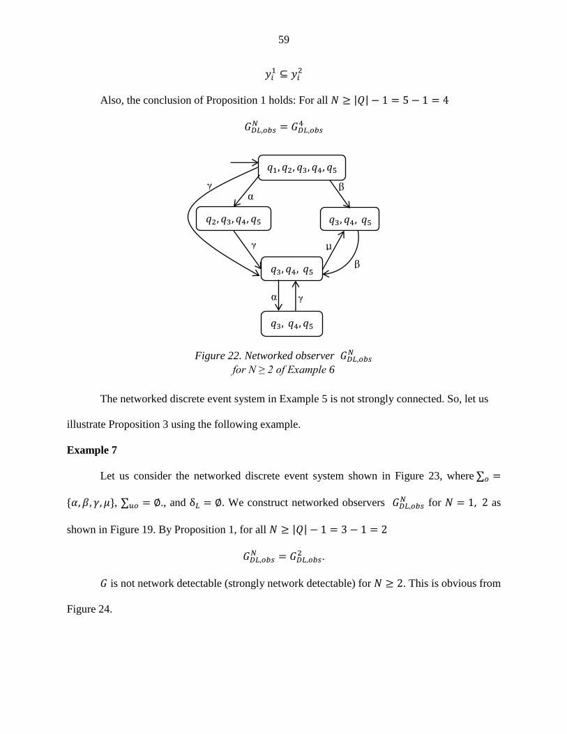
59

𝑦𝑖1 ⊆ 𝑦𝑖

2

Also, the conclusion of Proposition 1 holds: For all 𝑁 ≥ |𝑄| − 1 = 5 − 1 = 4


4

The networked discrete event system in Example 5 is not strongly connected. So, let us

illustrate Proposition 3 using the following example.

Example 7

Let us consider the networked discrete event system shown in Figure 23, where ∑𝑜 =

{𝛼, 𝛽, 𝛾, 𝜇}, ∑𝑢𝑜 = ∅., and δ𝐿 = ∅. We construct networked observers 𝐺𝐷𝐿,𝑜𝑏𝑠𝑁 for 𝑁 = 1, 2 as

shown in Figure 19. By Proposition 1, for all 𝑁 ≥ |𝑄| − 1 = 3 − 1 = 2


2 .

𝐺 is not network detectable (strongly network detectable) for 𝑁 ≥ 2. This is obvious from

Figure 24.

α γ

α β

𝑞1, 𝑞2, 𝑞3, 𝑞4, 𝑞5

𝑞3, 𝑞4, 𝑞5 𝑞2, 𝑞3, 𝑞4, 𝑞5

𝑞3, 𝑞4, 𝑞5

𝑞3, 𝑞4, 𝑞5

γ

γ

β

µ

Figure 22. Networked observer 𝐺𝐷𝐿,𝑜𝑏𝑠𝑁

for N ≥ 2 of Example 6

60

Figure 23. Networked discrete

event system G of Example 7

Figure 24. Networked observers 𝐺𝐷𝐿,𝑜𝑏𝑠𝑁 for N=1,2 of Example 7

γ

µ α

𝑞1

𝑞2 𝑞3

β

γ

µ α

𝑞1, 𝑞2

𝑞1, 𝑞2, 𝑞3 𝑞1, 𝑞3

β

γ

µ α

𝑞1, 𝑞2, 𝑞3

𝑞1, 𝑞2, 𝑞3 𝑞1, 𝑞2, 𝑞3

β

a. N=1 b. N=2

61

CHAPTER 6 I-DETECTABILITY OF NETWORKED DISCRETE EVENT

SYSTEMS

In our pervious chapters, we talked about state estimation of the current state of the system.

current state estimation is important for some types of the system, such as determining the current

state of a train. However, in some cases, it is important to know the initial state of the system

instead of current state. Initial state detectability, or simply I-detectability, is very important when

we need to determine the state of the system after a failure. When a failure happens in a system, it

is required to know the initial state of the system that led to that failure to be able the repair it. Like

in debugging a software, the programmer needs to know the last instruction executed before the

results are not as expected. I-detectability is required whenever we need to determine the state of

the system in some past time. checking I-detectability of a system is not always possible because

it depends on the system itself. For some systems, I-detectability can be checked for all trajectories

of the system, and this called strong I-detectable. However, in other cases, we can only determine

I-detectability for some trajectories of the system, and we call it weak I-detectability. Formally, I-

detectability is defined as the ability to detect the initial state of the system after finite number of

event observations. In [73], Shu and Lin, has investigated I-detectability of discrete event systems.

They formally defined weak and strong I-detectabilities as following:

Weak I-Detectability [73]

A nondeterministic discrete event system G is weakly I-detectable with respect to 𝑃 if we

can determine, after a finite event observation, the initial state of the system for some trajectories

of the system. That is

(∃𝑛 ∈ ℕ)(∃𝑠 ∈ 𝐿𝜔(𝐺))(∀𝑢 ∈ Pr(𝑠))|𝑃(𝑢)| > 𝑛 ⇒ |𝐼(𝑄0, 𝑃(𝑢))| = 1.

Strong I-Detectability [73]

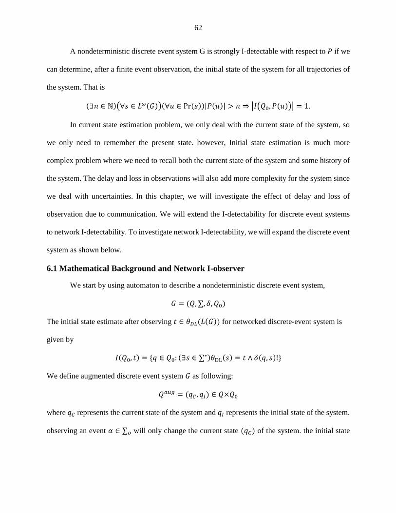
62

A nondeterministic discrete event system G is strongly I-detectable with respect to 𝑃 if we

can determine, after a finite event observation, the initial state of the system for all trajectories of

the system. That is

(∃𝑛 ∈ ℕ)(∀𝑠 ∈ 𝐿𝜔(𝐺))(∀𝑢 ∈ Pr(𝑠))|𝑃(𝑢)| > 𝑛 ⇒ |𝐼(𝑄0, 𝑃(𝑢))| = 1.

In current state estimation problem, we only deal with the current state of the system, so

we only need to remember the present state. however, Initial state estimation is much more

complex problem where we need to recall both the current state of the system and some history of

the system. The delay and loss in observations will also add more complexity for the system since

we deal with uncertainties. In this chapter, we will investigate the effect of delay and loss of

observation due to communication. We will extend the I-detectability for discrete event systems

to network I-detectability. To investigate network I-detectability, we will expand the discrete event

system as shown below.

6.1 Mathematical Background and Network I-observer

We start by using automaton to describe a nondeterministic discrete event system,

𝐺 = (𝑄, ∑, 𝛿, 𝑄0)

The initial state estimate after observing 𝑡 ∈ 휃𝐷𝐿(𝐿(𝐺)) for networked discrete-event system is

given by

𝐼(𝑄0, 𝑡) = {𝑞 ∈ 𝑄0: (∃𝑠 ∈ ∑∗)휃DL(𝑠) = 𝑡 ∧ 𝛿(𝑞, 𝑠)!}

We define augmented discrete event system 𝐺 as following:

𝑄𝑎𝑢𝑔 = (𝑞𝐶 , 𝑞𝐼) ∈ 𝑄×𝑄0

where 𝑞𝐶 represents the current state of the system and 𝑞𝐼 represents the initial state of the system.

observing an event 𝛼 ∈ ∑𝑜 will only change the current state (𝑞𝐶) of the system. the initial state

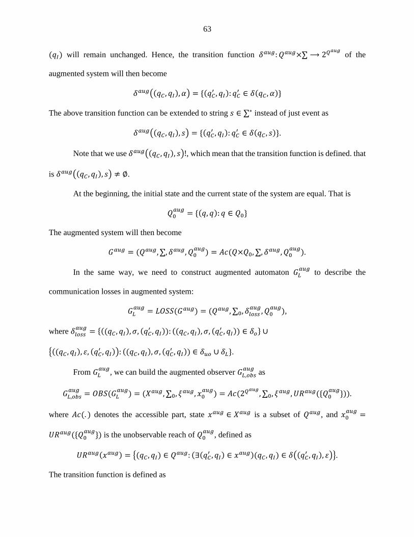
63

(𝑞𝐼) will remain unchanged. Hence, the transition function 𝛿𝑎𝑢𝑔: 𝑄𝑎𝑢𝑔×∑ ⟶ 2𝑄𝑎𝑢𝑔 of the

augmented system will then become

𝛿𝑎𝑢𝑔((𝑞𝐶 , 𝑞𝐼), 𝛼) = {(𝑞𝐶′ , 𝑞𝐼): 𝑞𝐶

′ ∈ 𝛿(𝑞𝐶 , 𝛼)}

The above transition function can be extended to string 𝑠 ∈ ∑∗ instead of just event as

𝛿𝑎𝑢𝑔((𝑞𝐶 , 𝑞𝐼), 𝑠) = {(𝑞𝐶′ , 𝑞𝐼): 𝑞𝐶

′ ∈ 𝛿(𝑞𝐶 , 𝑠)}.

Note that we use 𝛿𝑎𝑢𝑔((𝑞𝐶 , 𝑞𝐼), 𝑠)!, which mean that the transition function is defined. that

is 𝛿𝑎𝑢𝑔((𝑞𝐶 , 𝑞𝐼), 𝑠) ≠ ∅.

At the beginning, the initial state and the current state of the system are equal. That is

𝑄0𝑎𝑢𝑔

= {(𝑞, 𝑞): 𝑞 ∈ 𝑄0}

The augmented system will then become

𝐺𝑎𝑢𝑔 = (𝑄𝑎𝑢𝑔, ∑, 𝛿𝑎𝑢𝑔, 𝑄0𝑎𝑢𝑔

) = 𝐴𝑐(𝑄×𝑄0, ∑, 𝛿𝑎𝑢𝑔, 𝑄0𝑎𝑢𝑔

).

In the same way, we need to construct augmented automaton 𝐺𝐿𝑎𝑢𝑔

to describe the

communication losses in augmented system:

𝐺𝐿𝑎𝑢𝑔

= 𝐿𝑂𝑆𝑆(𝐺𝑎𝑢𝑔) = (𝑄𝑎𝑢𝑔, ∑0, 𝛿𝑙𝑜𝑠𝑠𝑎𝑢𝑔

, 𝑄0𝑎𝑢𝑔

),

where 𝛿𝑙𝑜𝑠𝑠𝑎𝑢𝑔

= {((𝑞𝐶 , 𝑞𝐼), 𝜎, (𝑞𝐶′ , 𝑞𝐼)): ((𝑞𝐶 , 𝑞𝐼), 𝜎, (𝑞𝐶

′ , 𝑞𝐼)) ∈ 𝛿𝑜} ∪

{((𝑞𝐶 , 𝑞𝐼), 휀, (𝑞𝐶′ , 𝑞𝐼)): ((𝑞𝐶 , 𝑞𝐼), 𝜎, (𝑞𝐶

′ , 𝑞𝐼)) ∈ 𝛿𝑢𝑜 ∪ 𝛿𝐿}.

From 𝐺𝐿𝑎𝑢𝑔

, we can build the augmented observer 𝐺𝐿,𝑜𝑏𝑠𝑎𝑢𝑔

as

𝐺𝐿,𝑜𝑏𝑠𝑎𝑢𝑔

= 𝑂𝐵𝑆(𝐺𝐿𝑎𝑢𝑔

) = (𝑋𝑎𝑢𝑔, ∑0, 𝜉𝑎𝑢𝑔, 𝑥0𝑎𝑢𝑔

) = 𝐴𝑐(2𝑄𝑎𝑢𝑔, ∑0, 𝜉𝑎𝑢𝑔, 𝑈𝑅𝑎𝑢𝑔({𝑄0

𝑎𝑢𝑔})).

where 𝐴𝑐(. ) denotes the accessible part, state 𝑥𝑎𝑢𝑔 ∈ 𝑋𝑎𝑢𝑔 is a subset of 𝑄𝑎𝑢𝑔, and 𝑥0𝑎𝑢𝑔

=

𝑈𝑅𝑎𝑢𝑔({𝑄0𝑎𝑢𝑔

}) is the unobservable reach of 𝑄0𝑎𝑢𝑔

, defined as

𝑈𝑅𝑎𝑢𝑔(𝑥𝑎𝑢𝑔) = {(𝑞𝐶 , 𝑞𝐼) ∈ 𝑄𝑎𝑢𝑔: (∃(𝑞𝐶′ , 𝑞𝐼) ∈ 𝑥𝑎𝑢𝑔)(𝑞𝐶 , 𝑞𝐼) ∈ 𝛿((𝑞𝐶

′ , 𝑞𝐼), 휀)}.


64

𝜉𝑎𝑢𝑔(𝑥𝑎𝑢𝑔, 𝛼) = 𝑈𝑅𝑎𝑢𝑔({(𝑞𝐶 , 𝑞𝐼) ∈ 𝑄𝑎𝑢𝑔: (∃(𝑞𝐶′ , 𝑞𝐼) ∈ 𝑥𝑎𝑢𝑔)(𝑞𝐶 , 𝑞𝐼) ∈ 𝛿((𝑞𝐶

′ , 𝑞𝐼), 𝜎)}).

Next, we extend each state 𝑥𝑎𝑢𝑔 ∈ 𝑋𝑎𝑢𝑔 to 𝑦𝑎𝑢𝑔 = 𝑅(𝑥𝑎𝑢𝑔). 𝑅(𝑥𝑎𝑢𝑔) denotes the set of states

that can be reached within N steps in 𝐺𝑎𝑢𝑔, that is,

𝑅(𝑥𝑎𝑢𝑔) = {(𝑞𝐶 , 𝑞𝐼) ∈ 𝑄𝑎𝑢𝑔: (∃(𝑞𝐶′ , 𝑞𝐼) ∈ 𝑥𝑎𝑢𝑔)(∃𝑠 ∈ ∑∗)|𝑠| ≤ 𝑁 ∧ 𝛿((𝑞𝐶

′ , 𝑞𝐼), 𝑠) = (𝑞𝐶 , 𝑞𝐼)}

Finally, the augmented networked I-observer 𝐺𝐷𝐿,𝑜𝑏𝑠𝑎𝑢𝑔

is defined as

𝐺𝐷𝐿,𝑜𝑏𝑠𝑎𝑢𝑔

= 𝐷𝐿(𝑂𝐵𝑆(𝐺𝐿𝑎𝑢𝑔

)) = (𝑌𝑎𝑢𝑔, ∑0, 휁𝑎𝑢𝑔, 𝑦0𝑎𝑢𝑔

).

In 𝐺𝐷𝐿,𝑜𝑏𝑠𝑎𝑢𝑔

, the state set 𝑌𝑎𝑢𝑔 is defined as follows. Denote 𝑋𝑎𝑢𝑔 = {𝑥1𝑎𝑢𝑔

, 𝑥2𝑎𝑢𝑔

, 𝑥3𝑎𝑢𝑔

, … … 𝑥𝑚𝑎𝑢𝑔

},

then 𝑌𝑎𝑢𝑔 = {𝑦1𝑎𝑢𝑔

, 𝑦2𝑎𝑢𝑔

, 𝑦3𝑎𝑢𝑔

, … … 𝑦𝑚𝑎𝑢𝑔

} with 𝑦𝑖𝑎𝑢𝑔

= 𝑅(𝑥𝑖𝑎𝑢𝑔

). The transition function

휁𝑎𝑢𝑔: 𝑌𝑎𝑢𝑔×∑0 → 𝑌𝑎𝑢𝑔 is defined for 𝑦𝑖𝑎𝑢𝑔

, 𝑦𝑗𝑎𝑢𝑔

∈ 𝑌𝑎𝑢𝑔 and ∈ ∑0, as

휁𝑎𝑢𝑔 = {(𝑦𝑖𝑎𝑢𝑔

, 𝜎, 𝑦𝑗𝑎𝑢𝑔

): (𝑥𝑖𝑎𝑢𝑔

, 𝜎, 𝑥𝑗𝑎𝑢𝑔

) ∈ 𝜉𝑎𝑢𝑔}

Theorem 9

The initial state estimation after observing 𝑡 ∈ 휃𝐷𝐿(𝐿(𝐺)) is given by

𝐼(𝑄0, 𝑡) = {𝑞𝐼 ∈ 𝑄0: (∃𝑞𝐶 ∈ 𝑄)(𝑞𝐼, 𝑞𝐶) ∈ 휁𝑎𝑢𝑔(𝑦0𝑎𝑢𝑔

, 𝑡)}

Proof

From the definition of the transition function, for 𝑠 ∈ ∑∗, we have

𝑞𝐶 ∈ 𝛿(𝑞𝐼 , 𝑠) ⇔ (𝑞𝐼 , 𝑞𝐶) ∈ 𝛿𝑎𝑢𝑔((𝑞𝐼 , 𝑞𝐼), 𝑠)

After observing 𝑡 ∈ 휃𝐷𝐿(𝐿(𝐺)), then

𝐼(𝑄0, 𝑡) = {𝑞𝐼 ∈ 𝑄0: (∃𝑠 ∈ ∑∗)휃DL(𝑠) = 𝑡 ∧ 𝛿(𝑞𝐼 , 𝑠)!}

= {𝑞𝐼 ∈ 𝑄0: (∃𝑞𝐶 ∈ 𝑄)(∃𝑠 ∈ ∑∗)휃DL(𝑠) = 𝑡 ∧ 𝑞𝐶 ∈ 𝛿(𝑞𝐼 , 𝑠)}

= {𝑞𝐼 ∈ 𝑄0: (∃𝑞𝐶 ∈ 𝑄)(∃𝑠 ∈ ∑∗)휃DL(𝑠) = 𝑡

∧ (𝑞𝐼 , 𝑞𝐶) ∈ 𝛿𝑎𝑢𝑔((𝑞𝐼 , 𝑞𝐼), 𝑠)}

= {𝑞𝐼 ∈ 𝑄0: (∃𝑞𝐶 ∈ 𝑄)(𝑞𝐼, 𝑞𝐶) ∈ 휁𝑎𝑢𝑔(𝑦0𝑎𝑢𝑔

, 𝑡)}

65

∎

6.2 Definitions of Network I-Detectabilities

We now define network I-detectabilities as follows.

Definition 9 (Network Weak I-Detectability)

A networked nondeterministic discrete event system G is weakly I-detectable with respect

to 휃𝐷𝐿if we can determine, after a finite event observation, the initial state of the system for some

trajectories of the system. That is

(∃𝑛 ∈ ℕ)(∃𝑠 ∈ 𝐿𝜔(𝐺))(∃𝑡 ∈ 휃𝐷𝐿(𝑠))(∀𝑡′ ∈ 𝑃𝑟(𝑡))(|𝑡′| > 𝑛 ⇒ |𝐼(𝑄0, 𝑡′)| = 1).

Definition 10 (Network Strong I-Detectability)

A networked nondeterministic discrete event system G is strongly I-detectable with respect

to 휃𝐷𝐿if we can determine, after a finite event observation, the initial state of the system for all

trajectories of the system. That is

(∃𝑛 ∈ ℕ)(∀𝑠 ∈ 𝐿𝜔(𝐺))(∀𝑡 ∈ 휃𝐷𝐿(𝑠))(∀𝑡′ ∈ 𝑃𝑟(𝑡))(|𝑡′| > 𝑛 ⇒ |𝐼(𝑄0, 𝑡′)| = 1).

6.3 Checking Network I-detectabilities

The I-observability of the networked discrete event system will not be affected by the

delays of the event observation. In other words, the effect of delays will just delay the observer

from sensing the initial state one step depending on the upper delay bound N. therefore, the I-

observer used to detect the initial state in [73] can be used to detect and observe the initial state

detectability for networked discrete event systems. Only observation losses can affect I-

detectabilities. To check network I-detectability of discrete event systems, we have the following

two cases.

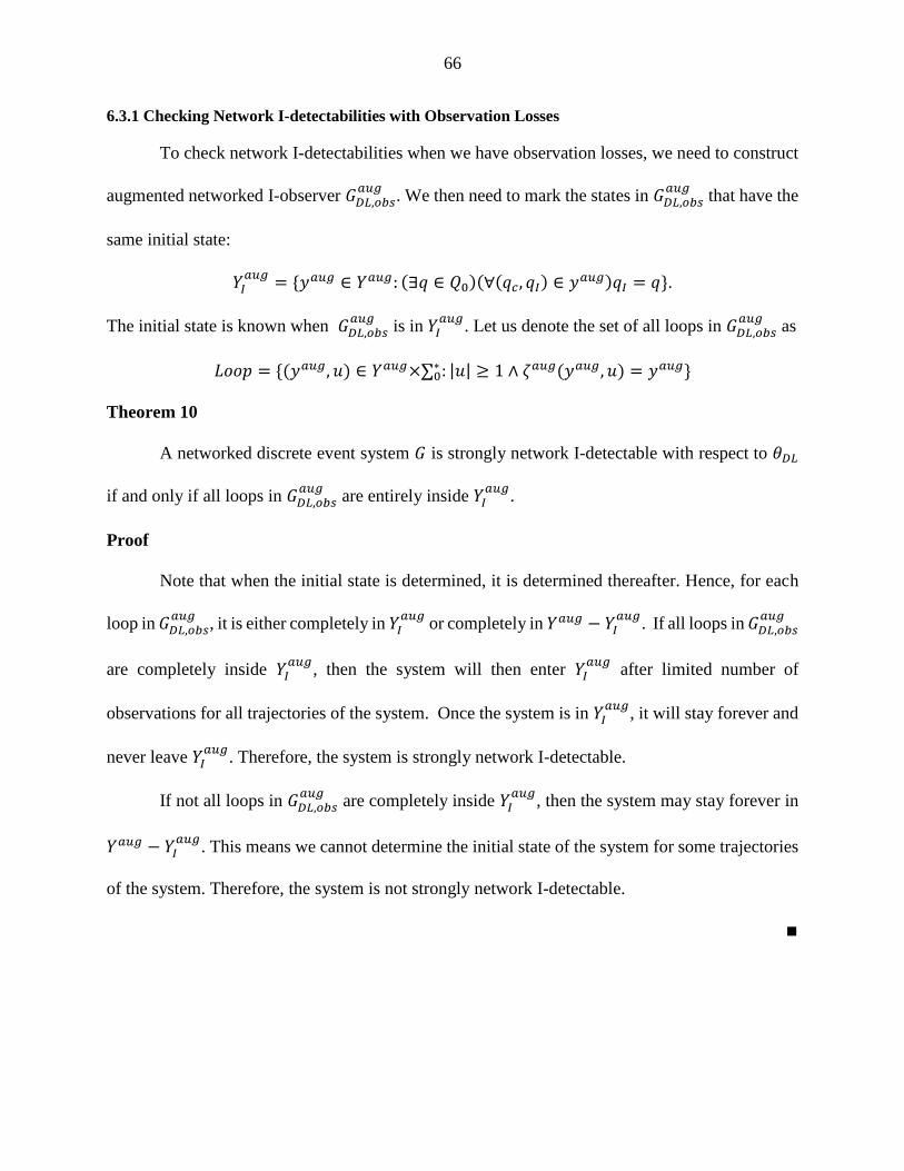
66

6.3.1 Checking Network I-detectabilities with Observation Losses

To check network I-detectabilities when we have observation losses, we need to construct

augmented networked I-observer 𝐺𝐷𝐿,𝑜𝑏𝑠𝑎𝑢𝑔

. We then need to mark the states in 𝐺𝐷𝐿,𝑜𝑏𝑠𝑎𝑢𝑔

that have the

same initial state:

𝑌𝐼𝑎𝑢𝑔

= {𝑦𝑎𝑢𝑔 ∈ 𝑌𝑎𝑢𝑔: (∃𝑞 ∈ 𝑄0)(∀(𝑞𝑐, 𝑞𝐼) ∈ 𝑦𝑎𝑢𝑔)𝑞𝐼 = 𝑞}.

The initial state is known when 𝐺𝐷𝐿,𝑜𝑏𝑠𝑎𝑢𝑔

is in 𝑌𝐼𝑎𝑢𝑔

. Let us denote the set of all loops in 𝐺𝐷𝐿,𝑜𝑏𝑠𝑎𝑢𝑔

as

𝐿𝑜𝑜𝑝 = {(𝑦𝑎𝑢𝑔, 𝑢) ∈ 𝑌𝑎𝑢𝑔×∑0∗ : |𝑢| ≥ 1 ∧ 휁𝑎𝑢𝑔(𝑦𝑎𝑢𝑔, 𝑢) = 𝑦𝑎𝑢𝑔}

Theorem 10

A networked discrete event system 𝐺 is strongly network I-detectable with respect to 휃𝐷𝐿

if and only if all loops in 𝐺𝐷𝐿,𝑜𝑏𝑠𝑎𝑢𝑔

are entirely inside 𝑌𝐼𝑎𝑢𝑔

.

Proof

Note that when the initial state is determined, it is determined thereafter. Hence, for each

loop in 𝐺𝐷𝐿,𝑜𝑏𝑠𝑎𝑢𝑔

, it is either completely in 𝑌𝐼𝑎𝑢𝑔

or completely in 𝑌𝑎𝑢𝑔 − 𝑌𝐼𝑎𝑢𝑔

. If all loops in 𝐺𝐷𝐿,𝑜𝑏𝑠𝑎𝑢𝑔

are completely inside 𝑌𝐼𝑎𝑢𝑔

, then the system will then enter 𝑌𝐼𝑎𝑢𝑔

after limited number of

observations for all trajectories of the system. Once the system is in 𝑌𝐼𝑎𝑢𝑔

, it will stay forever and

never leave 𝑌𝐼𝑎𝑢𝑔

. Therefore, the system is strongly network I-detectable.

If not all loops in 𝐺𝐷𝐿,𝑜𝑏𝑠𝑎𝑢𝑔

are completely inside 𝑌𝐼𝑎𝑢𝑔

, then the system may stay forever in

𝑌𝑎𝑢𝑔 − 𝑌𝐼𝑎𝑢𝑔

. This means we cannot determine the initial state of the system for some trajectories

of the system. Therefore, the system is not strongly network I-detectable.

∎

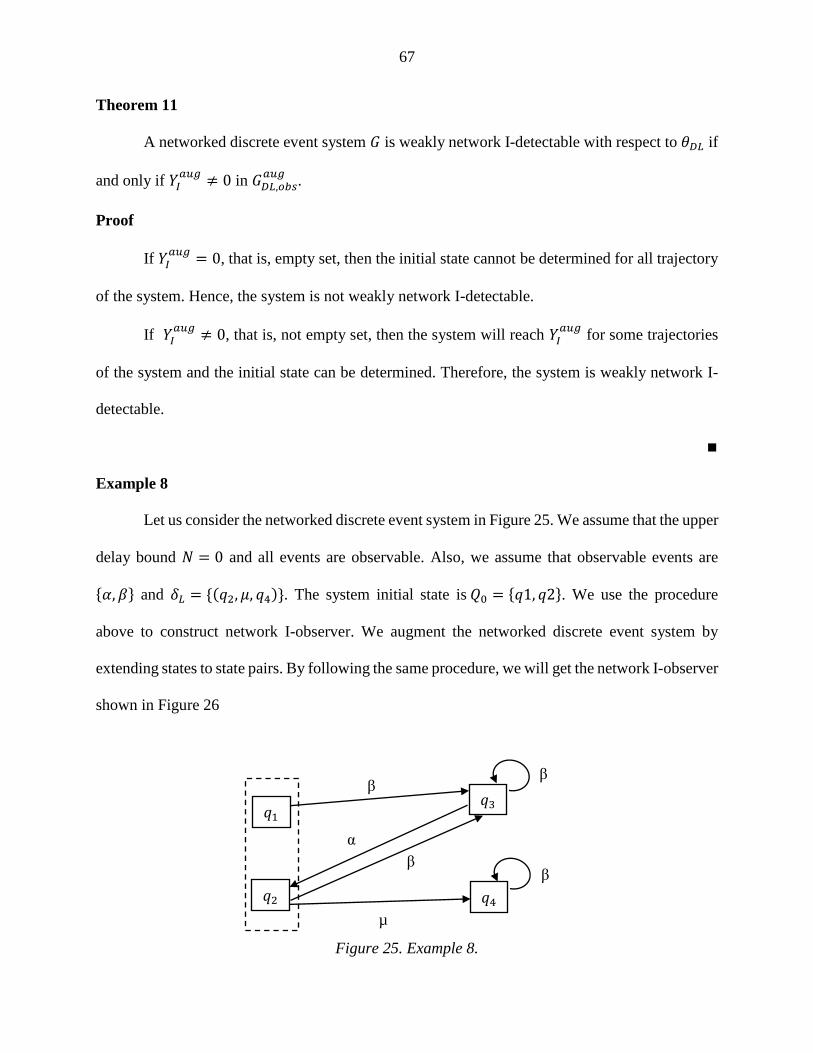
67

Theorem 11

A networked discrete event system 𝐺 is weakly network I-detectable with respect to 휃𝐷𝐿 if

and only if 𝑌𝐼𝑎𝑢𝑔

≠ 0 in 𝐺𝐷𝐿,𝑜𝑏𝑠𝑎𝑢𝑔

.

Proof

If 𝑌𝐼𝑎𝑢𝑔

= 0, that is, empty set, then the initial state cannot be determined for all trajectory

of the system. Hence, the system is not weakly network I-detectable.

If 𝑌𝐼𝑎𝑢𝑔

≠ 0, that is, not empty set, then the system will reach 𝑌𝐼𝑎𝑢𝑔

for some trajectories

of the system and the initial state can be determined. Therefore, the system is weakly network I-

detectable.

∎

Example 8

Let us consider the networked discrete event system in Figure 25. We assume that the upper

delay bound 𝑁 = 0 and all events are observable. Also, we assume that observable events are

{𝛼, 𝛽} and 𝛿𝐿 = {(𝑞2, 𝜇, 𝑞4)}. The system initial state is 𝑄0 = {𝑞1, 𝑞2}. We use the procedure

above to construct network I-observer. We augment the networked discrete event system by

extending states to state pairs. By following the same procedure, we will get the network I-observer

shown in Figure 26

β β

β

𝑞1

𝑞2

𝑞3

𝑞4

β

α

µ

Figure 25. Example 8.

68

6.3.2 Checking Network I-detectabilities without Observation Losses.

The I-detectability of a networked discrete event systems will not be affected by

observation delays. In other words, when there are no observation losses, network I-detectabilities

are equivalent to I-detectabilities. Hence, the I-observer used for checking I-detectabilities [73]

can be used to check network I-detectabilities. This is formally proved as follows.

Theorem 12

Assume that there are no observation losses in the system, that is, 𝛿𝑙𝑜𝑠𝑠 = ∅ and 𝛿𝑙𝑜𝑠𝑠𝑎𝑢𝑔

= ∅.

𝐺 is weakly network I-detectable if and only if 𝐺 is weakly I-detectable.

Proof

To prove that weakly network I-detectability (𝐴) is equivalent to weakly I-detectability

(𝐵), we need to prove that 𝐴 ⇔ 𝐵, where, by the definitions, 𝐴 and 𝐵 are as follows:

𝐴: (∃𝑛 ∈ ℕ)(∃𝑠 ∈ 𝐿𝜔(𝐺))(∃𝑡 ∈ 휃𝐷𝐿(𝑠))(∀𝑡′ ∈ 𝑃𝑟(𝑡))(|𝑡′| > 𝑛 ⇒ |𝐼(𝑄0, 𝑡′)| = 1)

Figure 26. Network I-Observer for Example 8.

(𝑞3, 𝑞1), (𝑞3, 𝑞2), (𝑞4, 𝑞1), (𝑞4, 𝑞2)

(𝑞1, 𝑞1), (𝑞2, 𝑞2), (𝑞4, 𝑞2)

(𝑞3, 𝑞1), (𝑞3, 𝑞2) (𝑞4, 𝑞2)

(𝑞2, 𝑞1), (𝑞2, 𝑞2), (𝑞4, 𝑞2), (𝑞4, 𝑞1)

β µ

β

α

(𝑞4, 𝑞1), (𝑞4, 𝑞2)

β µ

β

β α

µ β

69

𝐵: (∃𝑛 ∈ ℕ)(∃𝑠 ∈ 𝐿𝜔(𝐺))(∀𝑢 ∈ Pr(𝑠))|𝑃(𝑢)| > 𝑛 ⇒ |𝐼(𝑄0, 𝑃(𝑢))| = 1

(𝐴 ⇒ 𝐵)

Assume that 𝐴 is true, since

(∃𝑡 ∈ 휃𝐷𝐿(𝑢) = {𝑃(𝑢), 𝑃(𝑢−1), 𝑃(𝑢−2), … , 𝑃(𝑢−𝑁)})(|𝑡| > 𝑛 ⇒ |𝐼(𝑄0, 𝑡)| = 1)

In particular, for 𝑡 = 𝑃(𝑢)

|𝑡| > 𝑛 ⇒ |𝐼(𝑄0, 𝑡)| = 1, that is,

|𝑃(𝑢)| > |𝐼(𝑄0, 𝑡)| = 1

Hence 𝐵 is true.

(𝐴 ⇒ 𝐵)

Assume that 𝐵 is true, then

(∀𝑢 ∈ Pr(𝑠))(|𝑃(𝑢)| > 𝑛 ⇒ |𝐼(𝑄0, 𝑃(𝑢))| = 1)

(∀𝑢−1 ∈ Pr(𝑠))(|𝑃(𝑢−1)| > 𝑛 ⇒ |𝐼(𝑄0, 𝑃(𝑢))| = 1)

(∀𝑢−2 ∈ Pr(𝑠))(|𝑃(𝑢−2)| > 𝑛 ⇒ |𝐼(𝑄0, 𝑃(𝑢))| = 1)

(∀𝑢−𝑁 ∈ Pr(𝑠))(|𝑃(𝑢−𝑁)| > 𝑛 ⇒ |𝐼(𝑄0, 𝑃(𝑢))| = 1)

This implies

(∀𝑢 ∈ Pr(𝑠))(∀𝑡 ∈ {𝑃(𝑢), 𝑃(𝑢−1), 𝑃(𝑢−2), … , 𝑃(𝑢−𝑁)})(|𝑡| > 𝑛 ⇒ |𝐼(𝑄0, 𝑡)| = 1)

That is, 𝐴 is true.

If 𝛿𝑙𝑜𝑠𝑠 is equal to ∅, then 휃𝐷𝐿(𝑠) = {𝑃(𝑠), 𝑃(𝑠−1), 𝑃(𝑠−2), … , 𝑃(𝑠−𝑁)}. This means that

the projection will be equal natural. Therefore, 𝐴 will be a weakly network I-detectable. That

proves (𝐴 ⇒ 𝐵).

If (∃𝑛 ∈ ℕ)(∃𝑠 ∈ 𝐿𝜔(𝐺))(∀𝑢 ∈ Pr(𝑠))|𝑃(𝑢)| > 𝑛 ⇒ |𝐼(𝑄0, 𝑃(𝑢))| = 1 is a weakly I-

detectable and if the system introduced to a delay, it will take larger 𝑛 (𝑛 + 𝑁) for the system to

reach |𝐼(𝑄0, 𝑃(𝑢))| = 1.

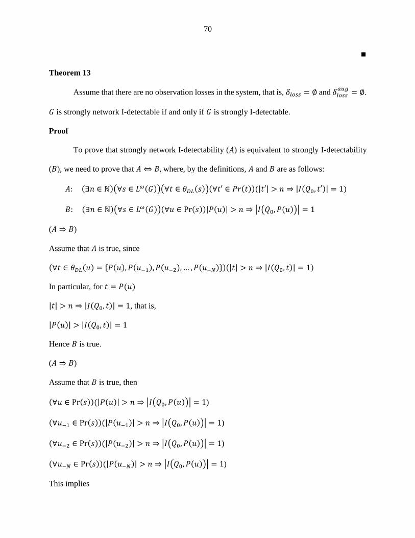
70

∎

Theorem 13

Assume that there are no observation losses in the system, that is, 𝛿𝑙𝑜𝑠𝑠 = ∅ and 𝛿𝑙𝑜𝑠𝑠𝑎𝑢𝑔

= ∅.

𝐺 is strongly network I-detectable if and only if 𝐺 is strongly I-detectable.

Proof

To prove that strongly network I-detectability (𝐴) is equivalent to strongly I-detectability

(𝐵), we need to prove that 𝐴 ⇔ 𝐵, where, by the definitions, 𝐴 and 𝐵 are as follows:

𝐴: (∃𝑛 ∈ ℕ)(∀𝑠 ∈ 𝐿𝜔(𝐺))(∀𝑡 ∈ 휃𝐷𝐿(𝑠))(∀𝑡′ ∈ 𝑃𝑟(𝑡))(|𝑡′| > 𝑛 ⇒ |𝐼(𝑄0, 𝑡′)| = 1)

𝐵: (∃𝑛 ∈ ℕ)(∀𝑠 ∈ 𝐿𝜔(𝐺))(∀𝑢 ∈ Pr(𝑠))|𝑃(𝑢)| > 𝑛 ⇒ |𝐼(𝑄0, 𝑃(𝑢))| = 1

(𝐴 ⇒ 𝐵)

Assume that 𝐴 is true, since

(∀𝑡 ∈ 휃𝐷𝐿(𝑢) = {𝑃(𝑢), 𝑃(𝑢−1), 𝑃(𝑢−2), … , 𝑃(𝑢−𝑁)})(|𝑡| > 𝑛 ⇒ |𝐼(𝑄0, 𝑡)| = 1)

In particular, for 𝑡 = 𝑃(𝑢)

|𝑡| > 𝑛 ⇒ |𝐼(𝑄0, 𝑡)| = 1, that is,

|𝑃(𝑢)| > |𝐼(𝑄0, 𝑡)| = 1

Hence 𝐵 is true.

(𝐴 ⇒ 𝐵)

Assume that 𝐵 is true, then

(∀𝑢 ∈ Pr(𝑠))(|𝑃(𝑢)| > 𝑛 ⇒ |𝐼(𝑄0, 𝑃(𝑢))| = 1)

(∀𝑢−1 ∈ Pr(𝑠))(|𝑃(𝑢−1)| > 𝑛 ⇒ |𝐼(𝑄0, 𝑃(𝑢))| = 1)

(∀𝑢−2 ∈ Pr(𝑠))(|𝑃(𝑢−2)| > 𝑛 ⇒ |𝐼(𝑄0, 𝑃(𝑢))| = 1)

(∀𝑢−𝑁 ∈ Pr(𝑠))(|𝑃(𝑢−𝑁)| > 𝑛 ⇒ |𝐼(𝑄0, 𝑃(𝑢))| = 1)

This implies

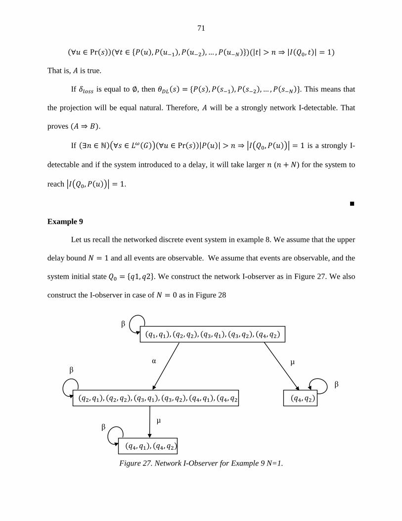
71

(∀𝑢 ∈ Pr(𝑠))(∀𝑡 ∈ {𝑃(𝑢), 𝑃(𝑢−1), 𝑃(𝑢−2), … , 𝑃(𝑢−𝑁)})(|𝑡| > 𝑛 ⇒ |𝐼(𝑄0, 𝑡)| = 1)

That is, 𝐴 is true.

If 𝛿𝑙𝑜𝑠𝑠 is equal to ∅, then 휃𝐷𝐿(𝑠) = {𝑃(𝑠), 𝑃(𝑠−1), 𝑃(𝑠−2), … , 𝑃(𝑠−𝑁)}. This means that

the projection will be equal natural. Therefore, 𝐴 will be a strongly network I-detectable. That

proves (𝐴 ⇒ 𝐵).

If (∃𝑛 ∈ ℕ)(∀𝑠 ∈ 𝐿𝜔(𝐺))(∀𝑢 ∈ Pr(𝑠))|𝑃(𝑢)| > 𝑛 ⇒ |𝐼(𝑄0, 𝑃(𝑢))| = 1 is a strongly I-

detectable and if the system introduced to a delay, it will take larger 𝑛 (𝑛 + 𝑁) for the system to

reach |𝐼(𝑄0, 𝑃(𝑢))| = 1.

∎

Example 9

Let us recall the networked discrete event system in example 8. We assume that the upper

delay bound 𝑁 = 1 and all events are observable. We assume that events are observable, and the

system initial state 𝑄0 = {𝑞1, 𝑞2}. We construct the network I-observer as in Figure 27. We also

construct the I-observer in case of 𝑁 = 0 as in Figure 28

(𝑞2, 𝑞1), (𝑞2, 𝑞2), (𝑞3, 𝑞1), (𝑞3, 𝑞2), (𝑞4, 𝑞1), (𝑞4, 𝑞2)

(𝑞1, 𝑞1), (𝑞2, 𝑞2), (𝑞3, 𝑞1), (𝑞3, 𝑞2), (𝑞4, 𝑞2)

(𝑞4, 𝑞2)

β

β

µ α

β

(𝑞4, 𝑞1), (𝑞4, 𝑞2)

µ β

Figure 27. Network I-Observer for Example 9 N=1.

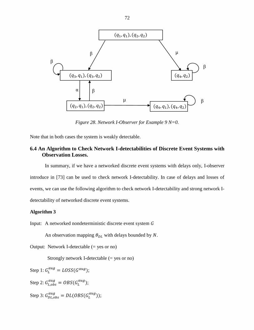
72

Note that in both cases the system is weakly detectable.

6.4 An Algorithm to Check Network I-detectabilities of Discrete Event Systems with

Observation Losses.

In summary, if we have a networked discrete event systems with delays only, I-observer

introduce in [73] can be used to check network I-detectability. In case of delays and losses of

events, we can use the following algorithm to check network I-detectability and strong network I-

detectability of networked discrete event systems.

Algorithm 3



Output: Network I-detectable (= yes or no)

Strongly network I-detectable (= yes or no)

Step 1: 𝐺𝐿𝑎𝑢𝑔

= 𝐿𝑂𝑆𝑆(𝐺𝑎𝑢𝑔);

Step 2: 𝐺𝐿,𝑜𝑏𝑠𝑎𝑢𝑔

= 𝑂𝐵𝑆(𝐺𝐿𝑎𝑢𝑔

);

Step 3: 𝐺𝐷𝐿,𝑜𝑏𝑠𝑎𝑢𝑔

= 𝐷𝐿(𝑂𝐵𝑆(𝐺𝐿𝑎𝑢𝑔

));

(𝑞3, 𝑞1), (𝑞3, 𝑞2)

(𝑞1, 𝑞1), (𝑞2, 𝑞2)

(𝑞4, 𝑞2)

β

β µ

α

β

(𝑞2, 𝑞1), (𝑞2, 𝑞2)

µ

β

(𝑞4, 𝑞1), (𝑞4, 𝑞2) β

Figure 28. Network I-Observer for Example 9 N=0.

73

Step 4: 𝑌𝐼𝑎𝑢𝑔

= {𝑦𝑎𝑢𝑔 ∈ 𝑌𝑎𝑢𝑔: (∃𝑞 ∈ 𝑄0)(∀(𝑞𝑐, 𝑞𝐼) ∈ 𝑦𝑎𝑢𝑔)𝑞𝐼 = 𝑞};

Step 5: 𝐿𝑜𝑜𝑝 = {(𝑦𝑎𝑢𝑔, 𝑢) ∈ 𝑌𝑎𝑢𝑔×∑0∗ : |𝑢| ≥ 1 ∧ 휁𝑎𝑢𝑔(𝑦𝑎𝑢𝑔, 𝑢) = 𝑦𝑎𝑢𝑔};

Step 6: If (∀(𝑦𝑎𝑢𝑔, 𝑢) ∈ 𝐿𝑜𝑜𝑝)(∀𝑤 ∈ ∑0∗ )휁𝑎𝑢𝑔(𝑦𝑎𝑢𝑔, 𝑤) ∈ 𝑌𝐼

𝑎𝑢𝑔 is true, then

Strongly network I-detectable = yes;

else

Strongly network I-detectable = no;

Step 7: If (∃(𝑦𝑎𝑢𝑔, 𝑢) ∈ 𝐿𝑜𝑜𝑝)(∀𝑤 ∈ 𝑃𝑟 (𝑢)) 휁𝑎𝑢𝑔(𝑦𝑎𝑢𝑔, 𝑤) ∈ 𝑌𝐼𝑎𝑢𝑔

is true, then

Network I-detectable = yes;

else

Network I-detectable = no.

74

CHAPTER 7 NETWORK CO-DETECTABILITY

In some applications, the observer is decentralized, so we have a set of local agents each

with limited observations. While the agents are not sharing date among themselves, if we can

determine the current and subsequent states all trajectories, then we have a system with strong co-

detectability. As you may know, every discrete event system is a unique case. Hence, it is hard

sometimes to detect the current and subsequent states for some systems for all trajectories of the

system. In such case, we may have a discrete event system with a weak co-detectability. In case of

multi-agents, determining the current and subsequent states of the system can be achieved with the

aid of limited observations of each agent. Co-detectability requires that we can determine the state

of the system by at least one agent. Formally, co-detectability can be defined as following:

We assume that I is the index of agents 𝐼 = {1,2,3, … 𝑛}.

𝑃𝑖 is the natural projection for an agent 𝐴𝑖.

𝑃𝑖 : ∑∗ → ∑𝑖,𝑜∗

𝑃𝑖 (𝜎) = {𝜎 𝑖𝑓 𝜎 ∈ ∑𝑖,𝑜

휀 𝑖𝑓 𝜎 ∉ ∑𝑖,𝑜 𝑃𝑖 (𝑠𝜎) = {

𝑃𝑖 (𝑠)𝜎 𝑖𝑓 𝜎 ∈ ∑𝑖,𝑜

𝑃𝑖 (𝑠) 𝑖𝑓 𝜎 ∉ ∑𝑖,𝑜

and

𝑅𝑖(𝑄′, 𝑡) is the set of all possible states after observing 𝑡 ∈ ∑𝑖,𝑜∗ for an agent 𝐴𝑖.

In this chapter, we investigate network co-detectability of discrete event systems. We

assume loss/delay between each agent and system. Therefore, this will introduce uncertainty in

detecting the current and subsequent states of the system.

Weak Co-detectability [75]

A discrete event system G is (weakly) co-detectable if, after a finite number of

observations, the current state and subsequent states of the system is known to at least one agent

for some trajectories of the system. Formally,

75

(∃𝑛 ∈ ℕ)(∃𝑠 ∈ 𝐿𝜔(𝐺))(∀𝑡 ∈ Pr(𝑠))|𝑃(𝑡)| > 𝑛 ⇒ (∃𝑖 ∈ 𝐼)|𝑅𝑖(𝑄0, 𝑃𝑖((𝑡))| = 1.

Strong Co-detectability [75]

A discrete event system G is strongly co-detectable if, after a finite number of observations,

the current state and subsequent states of the system is known to at least one agent for all

trajectories of the system. Formally,

(∃𝑛 ∈ ℕ)(∀𝑠 ∈ 𝐿𝜔(𝐺))(∀𝑡 ∈ Pr(𝑠))|𝑃(𝑡)| > 𝑛 ⇒ (∃𝑖 ∈ 𝐼)|𝑅𝑖(𝑄0, 𝑃𝑖((𝑡))| = 1.

Weak Periodic Co-detectability [75]

A discrete event system G is (weakly) periodically co-detectable if the current state of the

system is known periodically to at least one agent for some trajectories of the system. Formally,

(∃𝑛 ∈ ℕ)(∃𝑠 ∈ 𝐿𝜔(𝐺))(∀𝑡 ∈ Pr(𝑠))(∃𝑡′ ∈ ∑∗)𝑡𝑡′ ∈ Pr(𝑠) ∧

|𝑃(𝑡′)| < 𝑛 ∧ (∃𝑖 ∈ 𝐼)|𝑅𝑖(𝑄0, 𝑃𝑖((𝑡𝑡′))| = 1.

Strong Periodic Co-detectability [75]

A discrete event system G is strongly periodically co-detectable if the current state of the

system is known periodically to at least one agent for all trajectories of the system. Formally,

(∃𝑛 ∈ ℕ)(∀𝑠 ∈ 𝐿𝜔(𝐺))(∀𝑡 ∈ Pr(𝑠))(∃𝑡′ ∈ ∑∗)𝑡𝑡′ ∈ Pr(𝑠) ∧

|𝑃(𝑡′)| < 𝑛 ∧ (∃𝑖 ∈ 𝐼)|𝑅𝑖(𝑄0, 𝑃𝑖((𝑡𝑡′))| = 1.

7.1 Mathematical Background

The current state of the system will determine by these agents without sharing data. The

partial sensing capability for a specific agent 𝐴𝑖 is represented as observable events ∑𝑖,𝑜.

Obviously, the observable event of the networked discrete event system will be the union of all

observable events of the agents:

∑𝑜 = ⋃ ∑𝑖,𝑜

𝑖∈𝐼

76

We assume each agent 𝐴𝑖 has the same upper bound on delay. We denote that as 𝑁. This

assumption is made for simplicity.

The delay and lose projection for any agent 𝐴𝑖 is denoted as

휃𝑖,𝐷𝐿 = 휃𝑖,𝐿 ∘ 휃𝑖,𝐷

where

휃𝑖,𝐷: ∑∗ → 2∑∗.

and

휃𝑖,𝐿: 𝐿(𝐺) → 2∑∗𝑖,𝑜

We build the network observer for each agent as follows

𝐺𝑖,𝐿 = 𝐿𝑂𝑆𝑆(𝐺) = (𝑄, ∑𝑖,𝑜 , 𝛿𝑖,𝑙𝑜𝑠𝑠, 𝑄0),

where

𝛿𝑖,𝑙𝑜𝑠𝑠 = {(𝑞, 𝜎, 𝑞′): (𝑞, 𝜎, 𝑞′) ∈ 𝛿𝑖,𝑜} ∪ {(𝑞, 휀, 𝑞′): (𝑞, 𝜎, 𝑞′) ∈ 𝛿𝑖,𝑢𝑜 ∪ 𝛿𝑖,𝐿}.

We used δ to denote the set of all transitions in 𝐺: 𝛿 = {(𝑞, 𝜎, 𝑞′): 𝑞′ ∈ 𝛿(𝑞, 𝜎)}. The set

of observable transitions for an agent 𝐴𝑖 is denoted by 𝛿𝑖,𝑜 = {(𝑞, 𝜎, 𝑞′) ∈ 𝛿: 𝜎 ∈ ∑𝑖,𝑜} . The set of

unobservable transitions is denoted by 𝛿𝑖,𝑢𝑜 = {(𝑞, 𝜎, 𝑞′) ∈ 𝛿: 𝜎 ∈ ∑𝑖,𝑢𝑜} . Some observable

transitions may be lost in communication. These transitions are denoted by 𝛿𝑖,𝐿 (δ𝑖,𝐿 ⊆ δ𝑖,𝑜) [79,

103].

From 𝐺𝑖,𝐿, we can build the observer 𝐺𝐿,𝑜𝑏𝑠 as

𝐺𝑖,𝐿,𝑜𝑏𝑠 = 𝑂𝐵𝑆(𝐺𝑖,𝐿) = (𝑋𝑖, ∑𝑖,𝑜, 𝜉𝑖, 𝑥𝑖,0) = 𝐴𝑐(2𝑄 , ∑𝑖,𝑜 , 𝜉𝑖 , 𝑈𝑅𝑖({𝑄0})).

where 𝐴𝑐(. ) denotes the accessible part, state 𝑥𝑖 ∈ 𝑋𝑖 is a subset of 𝑄, and 𝑥𝑖,0 = 𝑈𝑅𝑖({𝑄0}) is the

unobservable reach of 𝑄0, defined as

𝑈𝑅𝑖(𝑥) = {𝑞 ∈ 𝑄: (∃𝑞′ ∈ 𝑥)𝑞 ∈ 𝛿𝑖,𝑙𝑜𝑠𝑠(𝑞′, 휀)}.


77

𝜉𝑖(𝑥, 𝜎) = 𝑈𝑅𝑖({𝑞 ∈ 𝑄: (∃𝑞′ ∈ 𝑥)𝑞 ∈ 𝛿𝑖,𝑙𝑜𝑠𝑠(𝑞′, 𝜎)}).

Next, we extend each state 𝑥𝑖 ∈ 𝑋𝑖 to 𝑦𝑖 = 𝑅(𝑥𝑖). 𝑅(𝑥𝑖) denotes the set of states that can be

reached within N steps in G, that is,

𝑅(𝑥𝑖) = {𝑞 ∈ 𝑄: (∃𝑞′ ∈ 𝑥𝑖)(∃𝑠 ∈ ∑∗)|𝑠| ≤ 𝑁 ∧ 𝛿(𝑞′, 𝑠) = 𝑞}

Finally, the networked observer is defined as

𝐺𝑖,𝐷𝐿,𝑜𝑏𝑠 = 𝐷𝐿(𝑂𝐵𝑆(𝐺𝑖,𝐿)) = (𝑌𝑖, ∑𝑖,𝑜, 휁𝑖 , 𝑦𝑖,0).

In 𝐺𝑖,𝐷𝐿,𝑜𝑏𝑠, the state set 𝑌𝑖 is defined as follows. Denote 𝑋 = {𝑥1, 𝑥2, 𝑥3, … … 𝑥𝑛}, then 𝑌𝑖 =

{𝑦1, 𝑦2, 𝑦3, … … 𝑦𝑛} with 𝑦𝑗 = 𝑅(𝑥𝑗). The transition function 휁𝑖: 𝑌𝑖×∑𝑖,𝑜 → 𝑌𝑖 is defined for

𝑦𝑗 , 𝑦𝑘 ∈ 𝑌𝑖 and ∈ ∑0, as

휁𝑖 = {(𝑦𝑗 , 𝜎, 𝑦𝑘): (𝑥𝑗 , 𝜎, 𝑥𝑘) ∈ 𝜉𝑖}

The networked observer can be used to find state estimates. In fact, it is proven by Lin

(2014) that

𝐸𝑖(𝑡) = 휁𝑖(𝑦𝑖,0, 𝑡)

We assume that the number of local agents is 𝑛. We also assume that there is an imaginary super-

agent that observes 𝐴. When this agent does not observe anything, this means no other agent can.

𝐺𝑐𝑜,𝐷𝐿,𝑜𝑏𝑠 = (𝑌, ∑𝑜 , 휁𝑐𝑜 , 𝑦0) = 𝐴𝑐(2𝑄×2𝑄×2𝑄× …×2𝑄 , ∑𝑜 , 휁𝑐𝑜 , 𝑦0)

where

𝑦0 = ( 𝑦0(1), 𝑦0(2), 𝑦0(3), … 𝑦0(𝑛), , 𝑦0(𝑛 + 1))

= (𝑈𝑅1(𝑄0), 𝑈𝑅2(𝑄0), 𝑈𝑅3(𝑄0), … 𝑈𝑅𝑧(𝑄0), 𝑈𝑅(𝑄0))

휁𝑐𝑜 is also a vector of 𝑛 + 1 elements.

7.2 Definitions of Network Co-Detectabilities

Now we define network co-detectabilities as follows.

Definition 11 (Network Co-detectability)

78

A networked discrete event system G is (weakly) network co-detectable if, after a finite

number of observations, the current state and subsequent states of the system is known to at least

one agent for some trajectories of the system. that is,

(∃𝑛 ∈ ℕ)(∃𝑠 ∈ 𝐿𝜔(𝐺))(∃𝑡 ∈ 휃𝐷𝐿(𝑠))(∀𝑡′ ∈ 𝑃𝑟(𝑡))(|𝑡′| > 𝑛 ⇒ (∃𝑖 ∈ 𝐼)|𝐸𝑖(𝑃𝑖(𝑡′))| = 1

Definition 12 (Strong Network Co-detectability)

A networked discrete event system G is strongly network co-detectable if, after a finite

number of observations, the current state and subsequent states of the system is known to at least

one agent for all trajectories of the system. that is,

(∃𝑛 ∈ ℕ)(∀𝑠 ∈ 𝐿𝜔(𝐺))(∀𝑡 ∈ 휃𝐷𝐿(𝑠))(∀𝑡′ ∈ 𝑃𝑟(𝑡))(|𝑡′| > 𝑛 ⇒ (∃𝑖 ∈ 𝐼)|𝐸𝑖(𝑃𝑖(𝑡′))| = 1

Definition 13 (Weak Network Periodic Co-detectability)

A networked discrete event system G is (weakly) periodically network co-detectable if the current

state of the system is known periodically to at least one agent for some trajectories of the system.

Formally,


(𝑡′𝑡′′ ∈ 𝑃𝑟(𝑡) ∧ |𝑡′′| < 𝑛 ∧ (∃𝑖 ∈ 𝐼)|𝐸𝑖(𝑃𝑖(𝑡′𝑡′′))| = 1).

Definition 14 (Strong Network Periodic Co-detectability)

A networked discrete event system G is strongly periodically network co-detectable if the current

state of the system is known periodically to at least one agent for all trajectories of the system.

Formally,


(𝑡′𝑡′′ ∈ 𝑃𝑟(𝑡) ∧ |𝑡′′| < 𝑛 ∧ (∃𝑖 ∈ 𝐼)|𝐸𝑖(𝑃𝑖(𝑡′𝑡′′))| = 1).

7.3 Checking Network Co-detectabilities

79

In order to check network co-detectabilities, we first construct networked observer

𝐺𝑐𝑜,𝐷𝐿,𝑜𝑏𝑠. We then mark the states in 𝐺𝑐𝑜,𝐷𝐿,𝑜𝑏𝑠 that contain a singleton state and denote the set

by:

𝑌𝑚 = {𝑦 ∈ 𝑌: (∃𝑦(𝑖))|𝑦(𝑖)| = 1 ∧ (1 ≤ 𝑖 ≤ 𝑛)}.

The state in 𝐺 is known when 𝐺𝑐𝑜,𝐷𝐿,𝑜𝑏𝑠 is in 𝑌𝑚. If that is the case, then there is at least one agent

that knows the current state of the system. We depend on loops to check co-detectabilities.

Therefore, Let us denote the set of all loops in 𝐺𝑐𝑜,𝐷𝐿,𝑜𝑏𝑠 as

𝐿𝑜𝑜𝑝 = {(𝑦, 𝑢) ∈ 𝑌×∑0∗ : |𝑢| ≥ 1 ∧ 휁𝑐𝑜(𝑦, 𝑢) = 𝑦}

Theorem 14

A networked nondeterministic discrete event system 𝐺 is strongly network co-detectable

with respect of a set of remote agents if and only if in the networked co-observer 𝐺𝑐𝑜,𝐷𝐿,𝑜𝑏𝑠,

(∀(𝑦, 𝑢) ∈ 𝐿𝑜𝑜𝑝)(∀𝑤 ∈ ∑0∗ ) 휁𝑐𝑜(𝑦, 𝑤) ∈ 𝑌𝑚.

In other words, any state reachable from any loop in 𝐺𝑐𝑜,𝐷𝐿,𝑜𝑏𝑠 is in 𝑌𝑚.

Theorem 15

A networked nondeterministic discrete event system 𝐺 is network co-detectable with

respect of a set of remote agents if and only if in the networked co-observer 𝐺𝑐𝑜,𝐷𝐿,𝑜𝑏𝑠,

(∃(𝑦, 𝑢) ∈ 𝐿𝑜𝑜𝑝)(∀𝑤 ∈ Pr (𝑢)) 휁𝑐𝑜(𝑦, 𝑤) ∈ 𝑌𝑚.

In other words, there are loops in 𝐺𝑐𝑜,𝐷𝐿,𝑜𝑏𝑠 which are completely inside 𝑌𝑚.

Theorem 16

A networked nondeterministic discrete event system G is strongly periodically network co-

detectable with respect of a set of remote agents if and only if in the networked co-observer

𝐺𝑐𝑜,𝐷𝐿,𝑜𝑏𝑠,

(∀(𝑦, 𝑢) ∈ 𝐿𝑜𝑜𝑝)(∃𝑤 ∈ Pr (u)) 휁𝑐𝑜(𝑦, 𝑤) ∈ 𝑌𝑚,

80

that is, every loop in 𝐺𝑐𝑜,𝐷𝐿,𝑜𝑏𝑠 must contain at least one state belonging to 𝑌𝑚.

Theorem 17

A networked nondeterministic discrete event system G is periodically network co-

detectable with respect of a set of remote agents if and only if in the networked co-observer

𝐺𝑐𝑜,𝐷𝐿,𝑜𝑏𝑠,

(∃(𝑦, 𝑢) ∈ 𝐿𝑜𝑜𝑝)(∃𝑤 ∈ Pr (u)) 휁𝑐𝑜(𝑦, 𝑤) ∈ 𝑌𝑚,

That is, there are loops in 𝐺𝑐𝑜,𝐷𝐿,𝑜𝑏𝑠 that include at least one state belonging to 𝑌𝑚.

Proofs for theorems 14, 15, 16, and 17 are similar to the proofs of theorems 1, 2, 3, and 4.

Therefore, proofs are omitted.

7.4 An Algorithm to Check Network Co-detectabilities of Discrete Event Systems

In summary, we can check network co-detectability, strong network co-detectability,

periodically network co-detectability, and strongly periodically network co-detectability using the

following algorithm

Algorithm 4


An observation mapping for each agent 휃𝑖,𝐷𝐿 with delays bounded by 𝑁𝑖.

Output: Network co-detectable (= yes or no)

Strongly network co-detectable (= yes or no)

Periodically network co-detectable (= yes or no)

Strongly periodically network co-detectable (= yes or no)

Step 1: 𝐺𝑖,𝐿 = 𝐿𝑂𝑆𝑆(𝐺);

Step 2: 𝐺𝑖,𝐿,𝑜𝑏𝑠 = 𝑂𝐵𝑆(𝐺𝑖,𝐿);

Step 3: 𝐺𝑐𝑜,𝐷𝐿,𝑜𝑏𝑠 = (𝑌, ∑𝑜 , 휁𝑐𝑜 , 𝑦0);

81

Step 4: 𝑌𝑚 = {𝑦 ∈ 𝑌: |𝑦| = 1};

Step 5: 𝑌𝑚 = {𝑦 ∈ 𝑌: (∃𝑦(𝑖))|𝑦(𝑖)| = 1 ∧ (1 ≤ 𝑖 ≤ 𝑛)};

Step 6: If (∀(𝑦, 𝑢) ∈ 𝐿𝑜𝑜𝑝)(∀𝑤 ∈ ∑0∗ ) 휁𝑐𝑜(𝑦, 𝑤) ∈ 𝑌𝑚 is true, then

Strongly network co-detectable = yes;

else

Strongly network co-detectable = no;

Step 7: If (∃(𝑦, 𝑢) ∈ 𝐿𝑜𝑜𝑝)(∀𝑤 ∈ 𝑃𝑟 (𝑢)) 휁𝑐𝑜(𝑦, 𝑤) ∈ 𝑌𝑚 is true, then

Network co-detectable = yes;

else

Network co-detectable = no.

Step 8: If (∀(𝑦, 𝑢) ∈ 𝐿𝑜𝑜𝑝)(∃𝑤 ∈ Pr (u)) 휁𝑐𝑜(𝑦, 𝑤) ∈ 𝑌𝑚 is true, then

Strongly periodically network co-detectable = yes;

else

Strongly periodically network co-detectable = no;

Step 9: If (∃(𝑦, 𝑢) ∈ 𝐿𝑜𝑜𝑝)(∃𝑤 ∈ Pr (u)) 휁𝑐𝑜(𝑦, 𝑤) ∈ 𝑌𝑚 is true, then

Periodically network co-detectable = yes;

else

Periodically network co-detectable = no.

82

CHAPTER 8 CONCLUSION

In this dissertation, we have defined network detectability, network D-detectability,

network I-detectability, and network co-detectability of discrete event systems. We derived

necessary and sufficient conditions for network detectability, network D-detectability, network I-

detectability, and network co-detectability. We developed algorithms to check all types of network

detectabilities. We also discussed and proved some properties of networked discrete event systems.

Also, many examples have been given to illustrate different types of network detectabilities.

83

REFERENCES

[1] C. Cassandras and S. Lafortune, Introduction to Discrete Event Systems, 2nd ed.: Springer,

2007.

[2] F. Lin and W. Wonham, "Decentralized supervisory control of discrete-event systems,"

Information Sciences vol. 44, pp. 199-224, 1988.

[3] P. Ramadge and W. Wonham, "Supervisory control of a class of discrete event processes,"

SIAM journal on control and optimization, vol. 25, pp. 206-230, 1987.

[4] R. Cieslak, C. Desclaux, A. S. Fawaz, and P. Varaiya, "Supervisory control of discrete-

event processes with partial observations," IEEE transactions on automatic control, vol.

33, pp. 249-260, 1988.

[5] A. F. Vaz and W. M. Wonham, "On supervisor reduction in discrete event systems," On

supervisor reduction in discrete event systems, vol. 44, pp. 475-491, 1986.

[6] J. N. Tsitsiklis, "On the control of discrete-event dynamical systems," Decision and

Control, 1987. 26th IEEE Conference on, vol. 26, pp. 419-422, 1987.

[7] F. Lin and W. Wonham, "On observability of discrete-event systems," Information

Sciences, vol. 44, pp. 173-198, 1988.

[8] J. S. Ostroff and W. M. Wonham, "A temporal logic approach to real time control," In

Decision and Control, 1985 24th IEEE Conference on, vol. 24, pp. 656-657, 1985.

[9] K. Rudie and W. Wonham, "Think globally, act locally: decentralized supervisory control,"

IEEE Transactions on Automatic Control vol. 37, pp. 1692-1708, 1992.

[10] M. Heymann and F. Lin, "On-line control of partially observed discrete event systems,"

Discrete Event Dynamic Systems: Theory and Applications vol. 4, pp. 221-236, 1994.

84

[11] S. Chung, S. Lafortune, and F. Lin, "Limited lookahead policies in supervisory control of

discrete event systems," IEEE Transactions on Automatic Control vol. 37, pp. 1921-1935,

1992.

[12] F. Lin, "Robust and adaptive supervisory control of discrete event systems," IEEE

Transactions on Automatic Control vol. 38, pp. 1848-1852, 1993.

[13] W. M. Wonham, "Towards an Abstract Internal Model Principle," IEEE Transactions on

Systems, Man, and Cybernetics, vol. 6, pp. 735-740, 1976.

[14] P. Ramadge, "Observability of discrete event systems," In 1986 25th IEEE Conference on

Decision and Control, vol. 25, pp. 1108-1112, 1986.

[15] C. Ozveren and A. Willsky, "Observability of discrete event dynamic systems," IEEE

Transactions on Automatic Control vol. 35, pp. 797-806, 1990.

[16] M. E. Merchant, "Production: A dynamic challenge: What's needed is flexibility Â¿ The

ability to manufacture efficiently a constantly changing variety of products," IEEE

spectrum, vol. 20, pp. 36-39, 1983.

[17] G. A. Frank, D. L. Franke, and W. F. Ingogly, "An architecture design and assessment

system," VLSI Design, vol. 6, pp. 30-50, 1985.

[18] W. B. Gevarter, "Expert systems: limited but powerful," IEEE, 1983.

[19] S. Shu and F. Lin, "Generalized detectability for discrete event systems," Systems &

Control Letters vol. 60, pp. 310-317, 2011.

[20] S. Shu, F. Lin, and H. Ying, "Detectability of discrete event systems," IEEE Transactions

on Automatic Control, vol. 52, pp. 2356-2359, 2007.

85

[21] M. Sampath, R. Sengupta, S. Lafortune, K. Sinnamohideen, and D. Teneketzis,

"Diagnosability of discrete event systems," IEEE Transactions on Automatic Control, vol.

40, pp. 1555-1575, 1995.

[22] M. Sampath, R. Sengupta, S. Lafortune, K. Sinnamohideen, and D. Teneketzis, "Failure

diagnosis using discrete event models," IEEE Transactions on Control System Technology,

vol. 4, pp. 105-124, 1996.

[23] T. S. Yoo and S. Lafortune, "Polynomial-time verification of diagnosability of partially

observed discrete-event systems," IEEE Transactions on automatic control, vol. 47, pp.

1491-1495, 2002.

[24] S. Jiang, Z. Huang, V. Chandra, and R. Kumar, "A polynomial algorithm for testing

diagnosability of discrete-event systems," EEE Transactions on Automatic Control, vol.

46, pp. 1318-1321, 2001.

[25] F. Lin, "Diagnosability of discrete event systems and its applications," Discrete Event

Dynamic Systems, vol. 4, pp. 197-212, 1994.

[26] R. Debouk, S. Lafortune, and D. Teneketzis, "Coordinated decentralized protocols for

failure diagnosis of discrete event systems," Decision and Control, 1998. Proceedings of

the 37th IEEE conference on, vol. 4, pp. 3763-3768, 1998.

[27] D. Thorsley and D. Teneketzis, "Diagnosability of stochastic discrete-event systems,"

IEEE Transactions on Automatic Control, vol. 50, pp. 476-492, 2005.

[28] M. Sampath, S. Lafortune, and D. Teneketzis, "Active diagnosis of discrete-event

systems," IEEE Transactions on Automatic Control, vol. 43, pp. 908-929, 1998.

[29] O. Contant, S. Lafortune, and D. Teneketzis, "Diagnosability of discrete event systems

with modular structure," Discrete Event Dynamic Systems, vol. 16, pp. 9-37, 2006.

86

[30] M. V. Moreira, T. C. Jesus, and J. C. Basilio, "Polynomial time verification of decentralized

diagnosability of discrete event systems," IEEE Transactions on Automatic Control, vol.

56, pp. 1679-1684, 2011.

[31] W. Qiu and R. Kumar, "Decentralized failure diagnosis of discrete event systems," IEEE

Transactions on Systems, Man, and Cybernetics-Part A: Systems and Humans, vol. 36, pp.

384-395, 2006.

[32] Y. Pencolé, "Diagnosability analysis of distributed discrete event systems," In Proceedings

of the 16th European Conference on Artificial Intelligence, pp. 38-42, 2004.

[33] S. Jiang and R. Kumar, "Failure diagnosis of discrete-event systems with linear-time

temporal logic specifications," IEEE Transactions on Automatic Control, vol. 49, pp. 934-

945, 2004.

[34] A. Ramirez-Trevino, E. Ruiz-Beltran, I. Rivera-Rangel, and E. Lopez-Mellado, "Online

fault diagnosis of discrete event systems. A Petri net-based approach," IEEE Transactions

on Automation Science and Engineering, vol. 4, pp. 31-39, 2007.

[35] A. Paoli and S. Lafortune, "Safe diagnosability for fault-tolerant supervision of discrete-

event systems," Automatica, vol. 41, pp. 1335-1347, 2005.

[36] F. Basile, P. Chiacchio, and G. De Tommasi, "An efficient approach for online diagnosis

of discrete event systems," IEEE Transactions on Automatic Control, vol. 54, pp. 748-759,

2009.

[37] S. Haar, A. Benveniste, E. Fabre, and C. Jard, "Partial order diagnosability of discrete event

systems using Petri net unfoldings," In Decision and Control, 2003. Proceedings. 42nd

IEEE Conference on, vol. 4, pp. 3748-3753, 2003.

87

[38] A. Benveniste, E. Fabre, S. Haar, and C. Jard, "Diagnosis of asynchronous discrete-event

systems: a net unfolding approach," IEEE Transactions on Automatic Control, vol. 48, pp.

714-727, 2003.

[39] T. Jéron, H. Marchand, S. Pinchinat, and M. O. Cordier, "Supervision patterns in discrete

event systems diagnosis," In Discrete event systems, 2006 8th international workshop on.

IEEE, pp. 262-268, 2006.

[40] A. Ramírez-Treviño, E. Ruiz-Beltran, I. Rivera-Rangel, and E. Lopez-Mellado,

"Diagnosability of discrete event systems: a petri net based approach," In Robotics and

Automation, 2004. Proceedings. ICRA'04. 2004 IEEE International Conference on. IEEE,

vol. 1, pp. 541-546, 2004.

[41] Y. Wang, T. S. Yoo, and S. Lafortune, "Diagnosis of discrete event systems using

decentralized architectures," Discrete Event Dynamic Systems, vol. 17, pp. 233-263, 2007.

[42] S. Jiang, R. Kumar, and H. E. Garcia, "Diagnosis of repeated/intermittent failures in

discrete event systems," IEEE transactions on robotics and automation, vol. 19, pp. 310-

323, 2003.

[43] S. Lafortune, D. Teneketzis, M. Sampath, R. Sengupta, and K. Sinnamohideen, "Failure

diagnosis of dynamic systems: An approach based on discrete event systems," In American

Control Conference, 2001. Proceedings of the 2001. IEEE, vol. 3, pp. 2058-2071, 2001.

[44] L. K. Carvalho, M. V. Moreira, and J. C. Basilio, "Generalized robust diagnosability of

discrete event systems," IFAC Proceedings Volumes, vol. 44, pp. 8737-8742, 2011.

[45] M. P. Cabasino, A. Giua, and C. Seatzu, "Diagnosability of discrete-event systems using

labeled Petri nets," IEEE Transactions on Automation Science and Engineering, vol. 11,

pp. 144-153, 2014.

88

[46] T. S. Yoo and S. Lafortune, "NP-completeness of sensor selection problems arising in

partially observed discrete-event systems," IEEE Transactions on Automatic Control, vol.

47, pp. 1495-1499, 2002.

[47] G. Lamperti and M. Zanella, "Diagnosis of discrete-event systems from uncertain temporal

observations," Artificial Intelligence, vol. 137, pp. 91-163, 2002.

[48] S. Bavishi and E. K. Chong, "Automated fault diagnosis using a discrete event systems

framework," In Intelligent Control, 1994., Proceedings of the 1994 IEEE International

Symposium on, pp. 213-218, 1994.

[49] M. O. Cordier, L. Travé-Massuyes, and X. Pucel, "Comparing diagnosability in continuous

and discrete-event systems," In Proceedings of the 17th International Workshop on

Principles of Diagnosis, vol. (DX-06), pp. 55-60, 2006.

[50] J. Chen and R. Kumar, "Polynomial test for stochastic diagnosability of discrete-event

systems," IEEE Transactions on Automation Science and Engineering, vol. 10, pp. 969-

979, 2013.

[51] S. H. Zad, R. H. Kwong, and W. M. Wonham, "Fault diagnosis in discrete-event systems:

Incorporating timing information," IEEE Transactions on Automatic Control, vol. 50, pp.

1010-1015, 2005.

[52] R. Kumar and S. Takai, "Inference-based ambiguity management in decentralized

decision-making: Decentralized diagnosis of discrete-event systems," IEEE Transactions

on Automation Science and Engineering, vol. 6, pp. 479-491, 2009.

[53] F. Lin and T. W. Lin, "Diagnosability of discrete event systems and its applications to

circuit testing," In Circuits and Systems, 1993., Proceedings of the 36th Midwest

Symposium on. IEEE, pp. 344-347, 1993.

89

[54] A. Paoli and S. Lafortune, "Safe diagnosability of discrete event systems," In Decision and

Control, 2003. Proceedings. 42nd IEEE Conference on, vol. 3, pp. 2658-2664, 2003.

[55] J. Zaytoon and S. Lafortune, "Overview of fault diagnosis methods for discrete event

systems," Annual Reviews in Control, vol. 37, pp. 308-320, 2013.

[56] J. C. Basilio and S. Lafortune, "Robust codiagnosability of discrete event systems," In

American Control Conference. IEEE, vol. ACC'09, pp. 2202-2209, 2009.

[57] J. Lunze and J. Schröder, "State observation and diagnosis of discrete-event systems

described by stochastic automata," Discrete Event Dynamic Systems, vol. 11, pp. 319-369,

2001.

[58] E. Kilic, "Diagnosability of fuzzy discrete event systems," Information Sciences, vol. 178,

pp. 858-870, 2008.

[59] Y. Pencolé and M. O. Cordier, "A formal framework for the decentralised diagnosis of

large scale discrete event systems and its application to telecommunication networks,"

Artificial Intelligence, vol. 164, pp. 121-170, 2005.

[60] Y. L. Chen and G. Provan, "Modeling and diagnosis of timed discrete event systems-a

factory automation example," American Control Conference, 1997. Proceedings of the

1997. IEEE, vol. 1, pp. 31-36, 1997.

[61] R. Debouk, S. Lafortune, and D. Teneketzis, "On the effect of communication delays in

failure diagnosis of decentralized discrete event systems," In Decision and Control, 2000.

Proceedings of the 39th IEEE Conference on, vol. 3, pp. 2245-2251, 2000.


Framework and model reduction," In Decision and Control, 1998. Proceedings of the 37th

IEEE Conference on, vol. 4, pp. 3769-3774, 1998.

90

[63] F. Liu and D. Qiu, "Diagnosability of fuzzy discrete-event systems: A fuzzy approach,"

IEEE Transactions on Fuzzy Systems, vol. 17, pp. 372-384, 2009.

[64] S. H. Zad, R. H. Kwong, and W. M. Wonham, "Fault diagnosis in timed discrete-event

systems," In Decision and Control, 1999. Proceedings of the 38th IEEE Conference on,

vol. 2, pp. 1756-1761, 1999.

[65] J. Dubreil, P. Darondeau, and H. Marchand, "Supervisory control for opacity," IEEE

Transactions on Automatic Control, vol. 55, pp. 1089-1100, 2010.

[66] R. Jacob, J. Lesage, and J. Faure, "Opacity of discrete event systems: models, validation

and quantification," IFAC-PapersOnLine vol. 48, pp. 174-181, 2015.

[67] F. Lin, "Opacity of discrete event systems and its applications," Automatica vol. 47, pp.

496-503, 2011.

[68] A. Saboori and C. Hadjicostis, "Notions of security and opacity in discrete event systems,"

Proceedings of the 46th IEEE Conference on Decision and Control pp. 5056-5061, 2007.

[69] A. Saboori and C. Hadjicostis, "Opacity-enforcing supervisory strategies for secure

discrete event systems," Proceedings of the 47th IEEE Conference on Decision and

Control, pp. 889-894, 2008.

[70] A. Saboori and C. Hadjicostis, "Verification of initial-state opacity in security applications

of discrete event systems," Information Sciences, vol. 246, pp. 115-132, 2013.

[71] Ben-Kalefa and F. Lin, "Supervisory control for opacity of discrete event systems,"

Communication, Control, and Computing (Allerton), 2011 49th Annual Allerton

Conference on. IEEE, pp. 1113-1119, 2011.

91

[72] W. Wang, S. Lafortune, and F. Lin, "An algorithm for calculating indistinguishable states

and clusters in finite-state automata with partially observable transitions," Systems &

Control Letters, vol. 56, pp. 656-661, 2007.

[73] S. Shu and F. Lin, "I-Detectability of Discrete-Event Systems," IEEE Transactions on

Automation Science and Engineering, vol. 10, pp. 187-196, 2013.

[74] S. Shu and F. Lin, "Delayed Detectability of Discrete Event Systems," IEEE Transactions

on Automatic Control, vol. 58, pp. 862-875, 2013.

[75] S. Shu and F. Lin, "Co-Detectability of Multi-Agent Discrete Event Systems," Proceedings

of 2011 Chinese Control and Decision Conference, pp. 1708-1713, 2011.

[76] R. Gupta and M. Chow, "Networked control system: Overview and research trends," IEEE

Transactions on Industrial Electronics, vol. 57, pp. 2527-2535, 2010.

[77] J. Hespanha, P. Naghshtabrizi, and Y. Xu, "A survey of recent results in networked control

systems," Proceedings of IEEE, vol. 95, pp. 138-162, 2007.

[78] S. Balemi, "Input/output discrete event processes and communication delays," Discrete

Event Dynamic Systems, vol. 4, pp. 41-85, 1994.

[79] F. Lin, "Control of networked discrete event systems: dealing with communication delays

and losses," SIAM Journal of Control and Optimization vol. 52, pp. 1276-1298, 2014.

[80] S. Park and K. Cho, "Supervisory control of discrete event systems with communication

delays and partial observations," Systems & Control Letters vol. 56, pp. 106-112, 2007.

[81] K. Rudie, S. Lafortune, and F. Lin, "Minimal communication in a distributed discrete event

system," IEEE Transactions on Automatic Control vol. 48, pp. 1965-1970, 2003.

92

[82] W. Wang, S. Lafortune, and F. Lin, "On the minimization of communication in networked

systems with a central station," Discrete Event Dynamic Systems: Theory and Applications

vol. 18, pp. 415-443, 2008.

[83] W. Wang, S. Lafortune, and F. Lin, "Minimization of communication of event occurrences

in acyclic discrete event systems," IEEE Transactions on Automatic Control, vol. 53, pp.

2197-2202, 2008.

[84] W. Wang, S. Lafortune, and F. Lin, "Minimization of dynamic sensor activation in discrete

event systems for the purpose of control," IEEE Transactions on Automatic Control, vol.

55, pp. 2447-2461, 2010.

[85] S. Park and K. Cho, "Decentralized supervisory control of discrete event systems with

communication delays based on conjunctive and permissive decision structure,"

Automatica, vol. 43, pp. 738-743, 2007.

[86] F. Lin, K. Rudie, and S. Lafortune, "Minimal communication for essential transitions in a

distributed discrete-event system," IEEE Transactions on Automatic Control vol.

52, pp. 1495-1502, 2007.

[87] L. Carvalho, J. Basilio, and M. Moreira, "Robust diagnosability of discrete event systems

subject to intermittent sensor failures," Proceedings of the 10th International Workshop on

Discrete Event Systems vol. 43, pp. 84-89, 2010.

[88] W. M. Wonham and P. J. Ramadge, "Modular supervisory control of discrete-event

systems," Mathematics of control, signals and systems vol. 1, pp. 13-30, 1988.

[89] P. J. Ramadge, "Control and supervision of discrete event processes," Ph.D Electrical

Engineering University of Toronto, 1983.

93

[90] W. M. Wonham and P. J. Ramadge, "On the supremal controllable sublanguage of a given

language," SIAM Journal on Control and Optimization, vol. 25, pp. 637-659, 1987.

[91] P. E. Caines, R. Greiner, and S. Wang, "Dynamical logic observers for finite automata," In

Decision and Control, 1988., Proceedings of the 27th IEEE Conference on, pp. 226-233,

1988.

[92] S. J. Rosenschein, "Formal theories of knowledge in AI and robotics," New generation

computing, vol. 3, pp. 345-357, 1985.

[93] S. J. Rosenschein and L. P. Kaelbling, "The synthesis of digital machines with provable

epistemic properties," Proceedings of the 1986 Conference on Theoretical aspects of

reasoning about knowledge, pp. 83-98, 1986.

[94] P. E. Caines, Linear stochastic systems vol. 11. New York: Wiley, 1988.

[95] G. Tadmor and O. Maimon, "Control of large discrete event systems: constructive

algorithms," IEEE Transactions on Automatic Control, vol. 34, pp. 1164-1168, 1989.

[96] L. Tobias and J. Scoggins, "Time-based air-traffic management using expert systems,"

IEEE Control Systems Magazine, vol. 7, pp. 23-29, 1987.

[97] F. Lin and H. Ying, "Modeling and control of fuzzy discrete event systems," IEEE

Transactions on Systems, Man, and Cybernetics, Part B (Cybernetics), vol. 32, pp. 408-

415, 2002.

[98] F. Lin, H. Ying, X. Luan, R. D. MacArthur, J. A. Cohn, D. Barth-Jones, et al., "Theory for

a control architecture of fuzzy discrete event systems for decision making," In Proceedings

of the 44th IEEE Conference on Decision and Control, 2005.

94


framework and model reduction," IEEE Transactions on Automatic Control, vol. 48, pp.

1199-1212, 2003.

[100] S. Jiang and R. Kumar, "Diagnosis of repeated failures for discrete event systems with

linear-time temporal-logic specifications," IEEE Transactions on Automation Science and

Engineering, vol. 3, pp. 47-59, 2006.

[101] M. Heymann and F. Lin, "Discrete-event control of nondeterministic systems," IEEE

Transactions on Automatic Control, vol. 43, pp. 3-17, 1998.

[102] J. G. Thistle and W. M. Wonham, "Control of infinite behavior of finite automata," SIAM

Journal on Control and Optimization, vol. 32, pp. 1075-1097, 1994.

[103] N. Ha, "Discrete-event systems abstractions for on-line and real-time hierarchical control,"

Doctor of Philosophy school of computer science and engineering Nanyang Technological

University 2016.

[104] V. Mitin, D. Romanov, and M. Polis, Modern advanced mathematics for engineers. New

York: John wiley & sons, INC, 2001.

[105] Y. Brave, "On stabilization of discrete event processes," in: Proceedings of CDC, pp.

2737–2743, 1989.

[106] C. M. Ozveren and A. S. Willsky, "Output stabilizability of discrete-event dynamic

systems," IEEE Transactions on Automatic Control, vol. 36, pp. 925-935, 1991.

[107] Y. Brave and M. Heymann, "Stabilization of discrete-event processes," International

Journal of Control, vol. 51, pp. 1101-1117, 1990.

95

ABSTRACT

ON DETECTABILITY OF NETWORKED DISCRETE EVENT SYSTEMS

by

YAZEED SASI

December 2017

Advisor: Dr. Feng Lin

Major: Electrical Engineering

Degree: Doctor of Philosophy

Detectability of discrete event systems, the ability to determine the current and subsequent

states, is very important in supervisory control and many other applications. So far only

detectability of non-networked discrete event systems has been defined and investigated. Non-

networked discrete event systems assume all the communication to be carried out on time without

any delays or losses. The assumption of reliable link is true when the distance of communication

is short; however, it is often violated in networked systems. In my dissertation, I investigate the

detectability for the networked discrete event systems. Because applications vary, we investigate

the four types of the network detectabilities: detectability, strong detectability, periodic

detectability, and strong periodic detectability. In addition, I will investigate the network D-

detectability, which is the ability to just distinguish certain pairs of states. As in non-networked

discrete event systems, I will extend the network detectability to network I-Detectability, and

network Co-detectability. Network I-detectability is defined as the ability of determining the initial

state of the system after finite numbers of event of observations when the system is subject to

communication delays and losses. Network Co-detectability, on the other hand, is defined as the

96

ability of determining the current state and subsequent states of the system with at least one agent

under communication delays losses. In each case, I will define and prove the necessary and

sufficient condition for the detectabilities if possible. In some cases, methods to check types of

network detectabilities are developed. Examples are also given to illustrate different types of

results.

97

AUTOBIOGRAPHICAL STATEMENT

Yazeed Sasi

Education

Yazeed Sasi received his B.Sc.Eng. degree in electrical engineering from El-Fateh University

(currently known as Tripoli University), Tripoli, Libya, in 2005. He received his M.Sc. degree in

electrical engineering from Wayne State University, Detroit, USA, in 2010. He is currently a PhD

candidate at Wayne State University, Detroit, USA.

From 2005 to 2006, he worked for Waha Oil Company, Tripoli, Libya. He then worked as a

teaching assistant in El-Fateh University from 2006 to 2008. His research interests are in the area

of discrete event systems and control.

He is a member of Tau Beta Pi - The Engineering Honor Society. He is also a member of Golden

Key International Honour Society.

Journal Paper

Y. Sasi, and F. Lin, “Detectability of networked discrete event systems,” Conditionally accepted

by Discrete Event Dynamic Systems.

On Detectability Of Networked Discrete Event Systems

Documents

Transcript of On Detectability Of Networked Discrete Event Systems