
On design of low order H-infinity controllers - DiVA
155
Linköping studies in science and technology. Dissertations. No. 1371 On design of low order H-infinity controllers Daniel Ankelhed Department of Electrical Engineering Linköping University, SE–581 83 Linköping, Sweden Linköping 2011
Transcript of On design of low order H-infinity controllers - DiVA

Linköping studies in science and technology. Dissertations.No. 1371
On design of low order H-infinitycontrollers
Daniel Ankelhed
Department of Electrical EngineeringLinköping University, SE–581 83 Linköping, Sweden
Linköping 2011

Cover illustration: An illustration of the feasible set for an H∞ synthesis prob-lem when the system has one state. Any point in the interior corresponds to acontroller with one state, i.e., a so-called full order controller. A point on thecurved boundary corresponds to a controller with zero states, i.e., a so-calledstatic controller or reduced order controller.
Linköping studies in science and technology. Dissertations.No. 1371
On design of low order H-infinity controllers
Daniel Ankelhed
[email protected] of Automatic Control
Department of Electrical EngineeringLinköping UniversitySE–581 83 Linköping
Sweden
ISBN 978-91-7393-157-1 ISSN 0345-7524
Copyright © 2011 Daniel Ankelhed
Printed by LiU-Tryck, Linköping, Sweden 2011

To U. Ché


Abstract
When designing controllers with robust performance and stabilization require-ments, H-infinity synthesis is a common tool to use. These controllers are oftenobtained by solving mathematical optimization problems. The controllers thatresult from these algorithms are typically of very high order, which complicatesimplementation. Low order controllers are usually desired, since they are con-sidered more reliable than high order controllers. However, if a constraint onthe maximum order of the controller is set that is lower than the order of the so-called augmented system, the optimization problem becomes nonconvex and itis relatively difficult to solve. This is true even when the order of the augmentedsystem is low.
In this thesis, optimization methods for solving these problems are considered.In contrast to other methods in the literature, the approach used in this thesis isbased on formulating the constraint on the maximum order of the controller as arational function in an equality constraint. Three methods are then suggested forsolving this smooth nonconvex optimization problem.
The first two methods use the fact that the rational function is nonnegative. Theproblem is then reformulated as an optimization problem where the rationalfunction is to be minimized over a convex set defined by linear matrix inequali-ties (LMIs). This problem is then solved using two different interior point meth-ods.
In the third method the problem is solved by using a partially augmented La-grangian formulation where the equality constraint is relaxed and incorporatedinto the objective function, but where the LMIs are kept as constraints. Again,the feasible set is convex and the objective function is nonconvex.
The proposed methods are evaluated and compared with two well-known meth-ods from the literature. The results indicate that the first two suggested methodsperform well especially when the number of states in the augmented system isless than 10 and 20, respectively. The third method has comparable performancewith two methods from literature when the number of states in the augmentedsystem is less than 25.
v


Populärvetenskaplig sammanfattning
Robust reglering är ett verktyg som används för att konstruera regulatorer tillsystem som har stora krav på tålighet mot parametervariationer och störningar.En metod för att konstruera dessa typer av robusta regulatorer är så kallad H-oändlighetssyntes. För att använda denna metod utgår man vanligen från ennominell modell av systemet som man utökar med olika viktfunktioner sommotsvaras av de krav på robusthet för parameterosäkerheter och störningar somställs på systemet. Detta får som följd att det utökade systemet ofta får mycket hö-gre komplexitet än det nominella systemet. Regulatorns komplexitet blir i regellika hög som det utökade systemets komplexitet. Inför man en övre gräns förden grad av komplexitet som tolereras, resulterar detta i mycket kompliceradeoptimeringsproblem som måste lösas för att en regulator ska kunna konstrueras,även i de fall då det nominella systemet har låg komplexitet. Att ha en regulatormed låg komplexitet är önskvärt då det förenklar implementering.
I denna avhandling föreslås tre metoder för att lösa denna typen av optimer-ingsproblem. Dessa tre metoder jämförs med två andra metoder beskrivna i lit-teraturen. Slutsatsen är att de föreslagna metoderna uppnår bra resultat så längesom systemen inte har alldeles för hög komplexitet.
vii


Acknowledgments
Wow, I have finally come to the end of this road! It has been a long trip and Iwould be lying if I said that I have enjoyed every part of it. However, I am so gladthat I made it all the way.
First, I would like to greatly thank my supervisors Anders Hansson and AndersHelmersson. Without your guidance and encouragement this trip would havebeen truly impossible.
Thank you Lennart Ljung for letting me join the automatic control group andthank you Svante Gunnarsson, Ulla Salaneck, Åsa Karmelind and Ninna Stens-gård for keeping track of everything here.
Extra thanks go to Anders Hansson, Anders Helmersson, Sina Khoshfetrat Paka-zad, Daniel Petersson and Johanna Wallén for your thorough proofreading of themanuscript of this thesis. Without your comments, this thesis would certainlybe painful to read. Writing the thesis would not have been so easy without theLATEX support from Gustaf Hendeby, Henrik Tidefelt and David Törnqvist. Thankyou!
A special thank you goes to Janne Harju Johansson with whom I shared officeduring my first three years here in the group. We started basically at the sametime and had many enjoyable discussions about courses, research, rock music,fiction literature or just anything. I would also like to give special thanks to mycolleagues André Carvalho Bittencourt, Sina Khoshfetrat Pakazad, Emre Özkanand Lubos Vaci. You always come up with fun ideas involving BBQ (regardlessof the temperature being minus a two digit value or not), drinking beer, visitrestaurants, watching great(?) movies or just hanging out. I would also like tothank the whole automatic control group for contributing to the nice atmosphere.The discussions in the coffee room can really turn a dull day into a great one!
I would also like to take the opportunity to thank my family. My parents Yvonneand Göte for your endless support, love and encouragement. Lars, always in agood mood and willing to help with anything. Joakim, Erik, Johanna and Jacob,when this book is finished I will hopefully have more time to spend time withyou.
Last, I would like to thank the Swedish research council for financial supportunder contract no. 60519401.
Linköping, May 2011
Daniel Ankelhed
ix


Contents
Notation xv
I Background
1 Introduction 31.1 Background . . . . . . . . . . . . . . . . . . . . . . . . . . . . . . . 3
1.1.1 Robust control . . . . . . . . . . . . . . . . . . . . . . . . . . 31.1.2 Previous work related to low order control design . . . . . 41.1.3 Controller reduction methods . . . . . . . . . . . . . . . . . 61.1.4 Motivation . . . . . . . . . . . . . . . . . . . . . . . . . . . . 6
1.2 Goals . . . . . . . . . . . . . . . . . . . . . . . . . . . . . . . . . . . 71.3 Publications . . . . . . . . . . . . . . . . . . . . . . . . . . . . . . . 71.4 Contributions . . . . . . . . . . . . . . . . . . . . . . . . . . . . . . 81.5 Thesis outline . . . . . . . . . . . . . . . . . . . . . . . . . . . . . . 9
2 Linear systems and H∞ synthesis 112.1 Linear system representation . . . . . . . . . . . . . . . . . . . . . . 11
2.1.1 System description . . . . . . . . . . . . . . . . . . . . . . . 122.1.2 Controller description . . . . . . . . . . . . . . . . . . . . . 122.1.3 Closed loop system description . . . . . . . . . . . . . . . . 12
2.2 The H∞ norm . . . . . . . . . . . . . . . . . . . . . . . . . . . . . . 132.3 H∞ controller synthesis . . . . . . . . . . . . . . . . . . . . . . . . . 152.4 Gramians and balanced realizations . . . . . . . . . . . . . . . . . . 182.5 Recovering the matrix P from X and Y . . . . . . . . . . . . . . . . 192.6 Obtaining the controller . . . . . . . . . . . . . . . . . . . . . . . . 202.7 A general algorithm for H∞ synthesis . . . . . . . . . . . . . . . . . 20
3 Optimization 213.1 Nonconvex optimization . . . . . . . . . . . . . . . . . . . . . . . . 21
3.1.1 Local methods . . . . . . . . . . . . . . . . . . . . . . . . . . 213.1.2 Global methods . . . . . . . . . . . . . . . . . . . . . . . . . 22
3.2 Convex optimization . . . . . . . . . . . . . . . . . . . . . . . . . . 22
xi
xii CONTENTS
3.3 Definitions . . . . . . . . . . . . . . . . . . . . . . . . . . . . . . . . 223.3.1 Convex sets and functions . . . . . . . . . . . . . . . . . . . 223.3.2 Cones . . . . . . . . . . . . . . . . . . . . . . . . . . . . . . . 233.3.3 Generalized inequalities . . . . . . . . . . . . . . . . . . . . 243.3.4 Logarithmic barrier function and the central path . . . . . 24
3.4 First order optimality conditions . . . . . . . . . . . . . . . . . . . 253.5 Unconstrained optimization . . . . . . . . . . . . . . . . . . . . . . 26
3.5.1 Newton’s method . . . . . . . . . . . . . . . . . . . . . . . . 263.5.2 Line search . . . . . . . . . . . . . . . . . . . . . . . . . . . . 283.5.3 Hessian modifications . . . . . . . . . . . . . . . . . . . . . 293.5.4 Newton’s method with Hessian modification . . . . . . . . 303.5.5 Quasi-Newton methods . . . . . . . . . . . . . . . . . . . . 30
3.6 Constrained optimization . . . . . . . . . . . . . . . . . . . . . . . . 323.6.1 Newton’s method for nonlinear equations . . . . . . . . . . 333.6.2 Central path . . . . . . . . . . . . . . . . . . . . . . . . . . . 333.6.3 A generic primal-dual interior point method . . . . . . . . 35
3.7 Penalty methods and augmented Lagrangian methods . . . . . . . 353.7.1 The quadratic penalty method . . . . . . . . . . . . . . . . . 353.7.2 The augmented Lagrangian method . . . . . . . . . . . . . 36
4 The characteristic polynomial and rank constraints 394.1 A polynomial criterion . . . . . . . . . . . . . . . . . . . . . . . . . 394.2 Replacing the rank constraint . . . . . . . . . . . . . . . . . . . . . 404.3 Problem reformulations . . . . . . . . . . . . . . . . . . . . . . . . . 42
4.3.1 An optimization problem formulation . . . . . . . . . . . . 424.3.2 A reformulation of the LMI constraints . . . . . . . . . . . . 42
4.4 Computing the characteristic polynomial of I − XY and its deriva-tives . . . . . . . . . . . . . . . . . . . . . . . . . . . . . . . . . . . . 434.4.1 Derivative calculations . . . . . . . . . . . . . . . . . . . . . 434.4.2 Computational complexity . . . . . . . . . . . . . . . . . . . 454.4.3 Derivatives of quotient . . . . . . . . . . . . . . . . . . . . . 45
4.5 Formulating a dynamic controller problem as a static controllerproblem . . . . . . . . . . . . . . . . . . . . . . . . . . . . . . . . . . 46
II Methods
5 A primal logarithmic barrier method 515.1 Introduction . . . . . . . . . . . . . . . . . . . . . . . . . . . . . . . 515.2 Problem formulation . . . . . . . . . . . . . . . . . . . . . . . . . . 525.3 Using the logarithmic barrier formulation . . . . . . . . . . . . . . 525.4 An extra barrier function . . . . . . . . . . . . . . . . . . . . . . . . 535.5 Outlining a barrier based method . . . . . . . . . . . . . . . . . . . 54
5.5.1 Initial point calculation . . . . . . . . . . . . . . . . . . . . . 555.5.2 Solving the main, nonconvex problem . . . . . . . . . . . . 555.5.3 Stopping criteria . . . . . . . . . . . . . . . . . . . . . . . . 57

CONTENTS xiii
5.6 The logarithmic barrier based algorithm . . . . . . . . . . . . . . . 575.6.1 Optimality of the solution . . . . . . . . . . . . . . . . . . . 575.6.2 Finding the controller . . . . . . . . . . . . . . . . . . . . . 585.6.3 Algorithm performance . . . . . . . . . . . . . . . . . . . . 58
5.7 Chapter summary . . . . . . . . . . . . . . . . . . . . . . . . . . . . 58
6 A primal-dual method 616.1 Introduction . . . . . . . . . . . . . . . . . . . . . . . . . . . . . . . 616.2 Problem formulation . . . . . . . . . . . . . . . . . . . . . . . . . . 626.3 Optimality conditions . . . . . . . . . . . . . . . . . . . . . . . . . . 636.4 Solving the KKT conditions . . . . . . . . . . . . . . . . . . . . . . 64
6.4.1 Central path . . . . . . . . . . . . . . . . . . . . . . . . . . . 646.4.2 Symmetry transformation . . . . . . . . . . . . . . . . . . . 646.4.3 Definitions . . . . . . . . . . . . . . . . . . . . . . . . . . . . 656.4.4 Computing the search direction . . . . . . . . . . . . . . . . 666.4.5 Choosing a positive definite approximation of the Hessian 676.4.6 Uniqueness of symmetric search directions . . . . . . . . . 686.4.7 Computing step lengths . . . . . . . . . . . . . . . . . . . . 68
6.5 A Mehrotra predictor-corrector method . . . . . . . . . . . . . . . . 696.5.1 Initial point calculation . . . . . . . . . . . . . . . . . . . . . 696.5.2 The predictor step . . . . . . . . . . . . . . . . . . . . . . . . 706.5.3 The corrector step . . . . . . . . . . . . . . . . . . . . . . . . 71
6.6 The primal-dual algorithm . . . . . . . . . . . . . . . . . . . . . . . 716.6.1 Finding the controller . . . . . . . . . . . . . . . . . . . . . 716.6.2 Algorithm performance . . . . . . . . . . . . . . . . . . . . 71
6.7 Chapter summary . . . . . . . . . . . . . . . . . . . . . . . . . . . . 72
7 A partially augmented Lagrangian method 737.1 Introduction . . . . . . . . . . . . . . . . . . . . . . . . . . . . . . . 737.2 Problem formulation . . . . . . . . . . . . . . . . . . . . . . . . . . 747.3 The partially augmented Lagrangian . . . . . . . . . . . . . . . . . 757.4 Calculating the search direction . . . . . . . . . . . . . . . . . . . . 76
7.4.1 Calculating the derivatives . . . . . . . . . . . . . . . . . . . 767.4.2 Hessian modifications . . . . . . . . . . . . . . . . . . . . . 76
7.5 An outline of the algorithm . . . . . . . . . . . . . . . . . . . . . . 777.6 Chapter summary . . . . . . . . . . . . . . . . . . . . . . . . . . . . 78
III Results and Conclusions
8 Numeric evaluations 838.1 Evaluation setup . . . . . . . . . . . . . . . . . . . . . . . . . . . . . 84
8.1.1 COMPleib . . . . . . . . . . . . . . . . . . . . . . . . . . . . 848.1.2 Hifoo . . . . . . . . . . . . . . . . . . . . . . . . . . . . . . 848.1.3 Hinfstruct . . . . . . . . . . . . . . . . . . . . . . . . . . . 85
8.2 The barrier method and the primal-dual method . . . . . . . . . . 858.2.1 Benchmarking problems . . . . . . . . . . . . . . . . . . . . 86

xiv CONTENTS
8.2.2 Evaluated methods . . . . . . . . . . . . . . . . . . . . . . . 868.2.3 The tests . . . . . . . . . . . . . . . . . . . . . . . . . . . . . 868.2.4 An in-depth study of AC8 and ROC8 . . . . . . . . . . . . . 878.2.5 Concluding the results . . . . . . . . . . . . . . . . . . . . . 908.2.6 Concluding remarks on the evaluation . . . . . . . . . . . . 94
8.3 The quasi-Newton method . . . . . . . . . . . . . . . . . . . . . . . 958.3.1 Benchmarking problems . . . . . . . . . . . . . . . . . . . . 958.3.2 Evaluated methods . . . . . . . . . . . . . . . . . . . . . . . 958.3.3 The tests . . . . . . . . . . . . . . . . . . . . . . . . . . . . . 968.3.4 A case study, AC6 . . . . . . . . . . . . . . . . . . . . . . . . 978.3.5 Extensive study . . . . . . . . . . . . . . . . . . . . . . . . . 978.3.6 Concluding remarks on the evaluation . . . . . . . . . . . . 1008.3.7 A comparison with the other methods . . . . . . . . . . . . 100
8.4 The partially augmented Lagrangian method . . . . . . . . . . . . 1008.4.1 Benchmarking problems . . . . . . . . . . . . . . . . . . . . 1018.4.2 Evaluated methods . . . . . . . . . . . . . . . . . . . . . . . 1018.4.3 The tests . . . . . . . . . . . . . . . . . . . . . . . . . . . . . 1018.4.4 Results and conclusions . . . . . . . . . . . . . . . . . . . . 102
9 Conclusions and further work 1059.1 Summary . . . . . . . . . . . . . . . . . . . . . . . . . . . . . . . . . 1059.2 Conclusions . . . . . . . . . . . . . . . . . . . . . . . . . . . . . . . 1069.3 Future work . . . . . . . . . . . . . . . . . . . . . . . . . . . . . . . 107
IV Tables with additional results
A Barrier, primal-dual and Hifoo 111A.1 Contents . . . . . . . . . . . . . . . . . . . . . . . . . . . . . . . . . 111A.2 Notation . . . . . . . . . . . . . . . . . . . . . . . . . . . . . . . . . 111
B The quasi-Newton method, AC6 119B.1 Contents . . . . . . . . . . . . . . . . . . . . . . . . . . . . . . . . . 119B.2 Notation . . . . . . . . . . . . . . . . . . . . . . . . . . . . . . . . . 119
C Barrier, primal-dual and quasi-Newton 121C.1 Contents . . . . . . . . . . . . . . . . . . . . . . . . . . . . . . . . . 121C.2 Quantifying the results . . . . . . . . . . . . . . . . . . . . . . . . . 121
Bibliography 125

Notation
Abbreviations
Abbreviation Meaning
BFGS Broyden, Fletcher, Goldfarb, ShannonBMI Bilinear matrix inequalityKKT Karush-Kuhn-TuckerLMI Linear matrix inequalityLQG Linear quadratic GaussianLTI Linear time-invariantNLP nonlinear problem/programNT Nesterov-ToddSDP Semidefinite program
SOCP Second order cone programSQP Sequential quadratic programmingSSP Sequential semidefinite programmingSVD Singular value decomposition
Sets
Notation Meaning
R Set of real numbersR+ Set of nonnegative real numbersR++ Set of positive real numbersRn Set of real-valued vectors with n rows
Rn×m Set of real-valued matrices with n rows andm columnsSn Set of symmetric matrices of size n × n
Sn+ The positive semidefinite cone of symmetric matrices
Sn++ The positive definite cone of symmetric matrices∅ The empty set
xv

xvi Notation
Symbols, operators and functions
Notation Meaning
H∞ H-infinityA � (�) 0 The matrix A is positive (semi)definiteA ≺ (�) 0 The matrix A is negative (semi)definiteA �K (�K ) 0 Generalized (strict) inequality with respect to the
cone Kx ≥ (>) 0 Element-wise (strict) inequalityAT Transpose of matrix AA−1 Inverse of matrix AA⊥ Orthogonal complement of matrix AAij Component (i, j) of matrix Axi The ith element of vector xx(i) Value of x at iteration i
det(A) Determinant of a matrix A ∈ Rn×nIn Identity matrix of size n × n〈A, B〉 Inner product of A and B‖x‖p p-norm of vector x‖A‖F Frobenius norm of matrix A‖G(s)‖∞ The H∞ norm of the continuous LTI system G(s)trace(A) Trace of a matrix ArangeA Range of a matrix A
kerA Kernel of a matrix AA ⊗ B Kronecker product of matrix A and BA ⊗s B Symmetric Kronecker product of matrix A and Bvec(A) Vectorization of matrix Asvec(A) Symmetric vectorization of matrix A ∈ Ssmat(a) The inverse operator of svec for a vector avech(A) Half-vectorization of matrix A ∈ Rn×n∇xf (x) The gradient of function f (x) with respect to x∇2xxf (x) The hessian of function f (x) with respect to x
min(a, b) The smallest of the scalars a and bargminx f (x) The minimizing argument of f (x)
diag(A) The diagonal elements of Ablkdiag(A, B, . . .) Block diagonal matrix with submatrices A, B, . . .
dom f (x) The domain of function f (x)

Part I
Background
1


1Introduction
In this thesis, the problem of designing low order H∞ controllers for continuouslinear time-invariant (LTI) systems is addressed. This chapter is structured asfollows. In Section 1.1 we discuss the motivation for the thesis and present im-portant work in the past that are related to this work. In Section 1.2 questionsare listed which we aim to answer in this thesis. A list of publications is givenin Section 1.3, where the author is the main contributor, and the contributionsare summarized in Section 1.4. We conclude this chapter with Section 1.5 bypresenting the outline of the remaining chapters of the thesis.
1.1 Background
We begin by a brief overview of the history of robust control. Then we presentwhat has been done in the past that is related to design of low order H∞ con-trollers, and we also very briefly discuss controller reduction methods. We con-clude this section with the motivation for the thesis.
1.1.1 Robust control
The development of robust control theory emerged during the 1980s and and acontributory factor certainly was the fact that the robustness of linear quadraticGaussian (LQG) controllers can get arbitrarily bad as reported in Doyle [1978].A few years later an important step in the development towards a robust controltheory was taken by Zames [1981], who introduced the concept of H∞ theory.
The H∞ synthesis, which is an important tool when solving robust control prob-lems, was a cumbersome problem to solve until a technique was presented inDoyle et al. [1989], which is based on solving two Riccati equations. Using this
3

4 1 Introduction
method, the robust design tools became much easier to use and gained popularity.Quite soon thereafter, in Gahinet and Apkarian [1994] and Iwasaki and Skelton[1994], linear matrix inequalities (LMIs) were found to be a suitable tool for solv-ing these kinds of problems. Also related problems, such as gain scheduling syn-thesis, see e.g. Packard [1994] and Helmersson [1995], fit into the LMI framework.In parallel to the theory for solving problems using LMIs, see e.g. the survey pa-pers by Vandenberghe and Boyd [1996] and Todd [2001], numerical methods forsolving LMIs were being developed.
Typical applications for robust control include systems that have high require-ments for robustness to parameter variations and high requirements for distur-bance rejection. The controllers that result from these algorithms are typicallyof very high order, which complicates implementation. However, if a constrainton the maximum order of the controller is set, that is lower than the order ofthe plant, the problem is no longer convex and is then relatively hard to solve.These problems become very complex, even when the order of the system to becontrolled is low. This motivates the use of efficient special purpose algorithmsthat can solve these kinds of problems.
1.1.2 Previous work related to low order control design
In Hyland and Bernstein [1984] necessary conditions for a reduced order con-troller to stabilize a system were stated. In Gahinet and Apkarian [1994] it wasshown that in order to find a reduced order controller using the LMI formulation,a rank constraint had to be satisfied. In Fu and Luo [1997] it was shown that thisproblem is so-called NP-hard. Many researchers were now focused on the issueof finding efficient methods to solve this hard problem.
The DK-iteration procedure became a popular method to solve robust controlproblems, see e.g. Doyle [1985]. In Iwasaki [1999] a similar method for low orderH∞ synthesis was presented, which solved the associated BMIs by fixing somevariables and optimizing on others in an alternating manner. The problems to besolved in each step were LMIs. One problem with these methods is that conver-gence is not guaranteed.
In Grigoriadis and Skelton [1996] an alternating projections algorithm was pre-sented. The algorithm seeks to locate an intersection of a convex set of LMIs and arank constraint. However, only local convergence is guaranteed for the low ordercase. Similar methods are presented in Beran [1997]. Other algorithms that ap-peared around this time were e.g. a min/max algorithm in Geromel et al. [1998],the XY-centering algorithm in Iwasaki and Skelton [1995], the potential reduc-tion algorithm in David [1994]. For a survey on static output feedback methods,see Syrmos et al. [1997].
Also some global methods began to appear. In Beran [1997] a branch and boundalgorithm for solving bilinear matrix inequalities (BMIs) was presented, whichdivides the set into several smaller ones where upper and lower bounds on theoptimal value are calculated. Similar approaches were presented in e.g. Goh et al.[1995], VanAntwerp et al. [1997] and Tuan and Apkarian [2000] and in the ref-

1.1 Background 5
erences therein. In Apkarian and Tuan [1999, 2000] an algorithm was presentedfor minimization of a nonconvex function over convex sets defined by LMIs. Theproblem was solved using a modified Frank-Wolfe method, see Frank and Wolfe[1956], combined with branch and bound methods.
Mesbahi and Papavassilopoulos [1997] showed how to compute lower and upperbound on the order of a dynamical output feedback controller that stabilizes agiven system by solving two semi-definite programs. In El Ghaoui et al. [1997],a cone complementarity linearization method was presented. In each iteration itsolved a problem involving a linearized nonconvex objective function subject toLMI constraints. Another method based on linearization is Leibfritz [2001].
A primal-dual method with a trust-region framework for solving nonconvex ro-bust control problems was suggested in Apkarian and Noll [2001]. A modi-fied version of the augmented Lagrangian method, the partially augmented La-grangian method was used in Fares et al. [2001] to solve a robust control prob-lem where the search direction was calculated using a modified Newton methodand a trust-region method. In Fares et al. [2002] the same formulation was usedbut solved using a sequential semidefinite programming approach. In Apkarianet al. [2003] and Apkarian et al. [2004] the low order H∞ problem was consid-ered, where in each iteration a convex SDP was solved in order to find a searchdirection.
A barrier method for solving problems involving BMIs was presented in Koc-vara et al. [2005] which is an extension of the so-called PBM method in Ben-Taland Zibulevsky [1997] to semidefinite programming. It uses a modified New-ton method to calculate the search direction. If ill-conditioning of the Hessianis detected, a slower but more robust trust-region method is used instead. Themethod was implemented in the software PENBMI. Other methods that attackthe BMI problem using local methods are e.g. Leibfritz and Mostafa [2002], Holet al. [2003] Kanev et al. [2004] and Thevenet et al. [2005]. For another overviewof earlier work in robust control, the introduction of Kanev et al. [2004] is recom-mended.
In Orsi et al. [2006], a method similar to the alternating projection algorithm inGrigoriadis and Skelton [1996] for finding intersections of sets defined by rankconstraints and LMIs is proposed. The method is implemented in the softwareLMIrank, see Orsi [2005].
In Apkarian and Noll [2006a] a nonsmooth, multi directional search approachwas considered that did not use the LMI formulation in Gahinet and Apkarian[1994] but instead searched directly in the controller parameter space. However,the method they used for solving this nonsmooth problem seem to have beenabandoned in favor for an approach using subgradient calculus, see e.g. Clarke[1990]. This approach was presented in Apkarian and Noll [2006b] and in 2010 itresulted in the code Hinfstruct, which is part of the Robust Control Tool-box in Matlab® version 7.11. In parallel, a code package for H-infinity fixedorder optimization, Hifoo, was being developed that considered the same non-

6 1 Introduction
smooth problem formulation as in Apkarian and Noll [2006b] but with anotherapproach. It was presented in Burke et al. [2006] and parts of its code are basedon gradient sampling, see Burke et al. [2005]. Further developments of Hifoowere presented in Gumussoy and Overton [2008a] and as presented in the paperby Arzelier et al. [2011] it now also includes methods for H2 controller synthesis.An advantage with these kind of nonsmooth methods, compared to LMI-basedmethods, is that they seem better fitted to handle systems with large dimensions.Another approach that directly minimizes an appropriate nonsmooth functionof the controller parameters is presented in Mammadov and Orsi [2005]. How-ever, it uses a different objective function compared to Burke et al. [2006] andApkarian and Noll [2006b].
New sufficient LMI conditions for low order controller design were presented inTrofino [2009], however some degree of conservatism was introduced due to theconditions only being sufficient. An algorithm that combines a randomization al-gorithm with a coordinate descent cross-decomposition algorithm is presented inArzelier et al. [2011]. The first part of the algorithm randomizes a set of feasiblepoints while the second part optimizes on a group of variables while keeping theother group of variables fixed and vice versa.
1.1.3 Controller reduction methods
A completely different approach worth mentioning is to compute the full ordercontroller and then apply model reduction techniques to get a low order con-troller. Some references on this approach are e.g. Enns [1984], Zhou [1995], God-dard and Glover [1998], and Kavranoğlu and Al-Amer [2001]. The results inGumussoy and Overton [2008a] indicate that controller reduction methods per-form best when the controller order is close to the order of the system. However,when the controller order is low compared to the order of the system, the resultsis in clear favor of optimization based methods such as Hifoo.
1.1.4 Motivation
To conclude the overview of related published work the following can be said.Several approaches to low order H∞ controller synthesis have been proposed inthe past. All methods have their advantages and disadvantages. None of theglobal methods have polynomial time complexity due to the NP-hardness of theproblem. As a result, these approaches require a large computational effort evenfor problems of modest size. Most of the local methods, on the other hand, arecomputationally fast but may not converge to the global optimum. The reasonfor this is the inherent nonconvexity of the problem. Some problem formulationsare “less” nonconvex than others, e.g. Apkarian et al. [2003], in the sense that itis only the objective function that is nonconvex while the constraints are convex.However, a drawback with the approach in Apkarian et al. [2003] is that thesystem is augmented with extra states in the case that a dynamic controller, i.e.,a controller with nonzero states, is searched for.
In Helmersson [2009] it was shown that the matrix rank constraint used in H∞

1.2 Goals 7
controller synthesis can be formulated as a polynomial constraint. This allowsnew approaches for low order H∞ controller design where a nonconvex functionis to be minimized over a convex set defined by LMIs. The order of the controllerin these approaches is decided by using a specific coefficient in a polynomial asobjective function instead of augmenting the system as is done in e.g. Apkarianet al. [2003]. Hopefully, this results in lower computational complexity and betterresults. In this thesis three different optimization algorithms for low order H∞controller synthesis will be investigated that use the formulation in Helmersson[2009].
1.2 Goals
In this thesis we aim to answer the following questions.
1. Which are currently the state of the art methods for low order H∞ controllersynthesis?
2. When using the reformulation of the rank constraint of a matrix as a quo-tient of two polynomials, see Helmersson [2009], in tandem with the classi-cal LMI formulation of the H∞ controller synthesis problem in Gahinet andApkarian [1994], what approaches can be used for solving the resulting op-timization problems? How well do these methods perform?
3. What are the advantages and disadvantages of using the LMI formulation ofthe H∞ controller synthesis problem compared to using nonsmooth meth-ods, e.g. the methods in Apkarian and Noll [2006b] and Gumussoy andOverton [2008a]?
1.3 Publications
The thesis is based on the following publications, where the author in the maincontributor.
D. Ankelhed, A. Helmersson, and A. Hansson. A primal-dual method forlow order H-infinity controller synthesis. In Proceedings of the 2009 IEEEConference on Decision and Control, Shanghai, China, Dec 2009.
D. Ankelhed, A. Helmersson, and A. Hansson. Additional numerical re-sults for the quasi-Newton interior point method for low order H-infinitycontroller synthesis. Technical Report LiTH-ISY-R-2964, Department of Au-tomatic Control, Linköping university, Sweden, 2010. URL http://www.control.isy.liu.se/publications/doc?id=2313.
D. Ankelhed, A. Helmersson, and A. Hansson. A quasi-Newton interior pointmethod for low order H-infinity controller synthesis. Accepted for publica-tion in IEEE Transactions on Automatic Control, 2011a.
D. Ankelhed. An efficient implementation of gradient and Hessian calcula-tions of the coefficients of the characteristic polynomial of I - XY. Techni-

8 1 Introduction
cal Report LiTH-ISY-R-2997, Department of Automatic Control, Linköpinguniversity, Sweden, 2011. URL http://www.control.isy.liu.se/publications/doc?id=2387.
D. Ankelhed, A. Helmersson, and A. Hansson. A partially augmented La-grangian algorithm for low order H-infinity controller synthesis using ratio-nal constraints. Submitted to the 2011 IEEE Conference on Decision andControl, December 2011b.
Some of the results in this thesis has previously been published in
D. Ankelhed. On low order controller synthesis using rational constraints.Licentiate thesis no. 1398, Department of Electrical Engineering, LinköpingUniversity, SE-581 83 Linköping, Sweden, Mar 2009.
Additionally, some work not directly related to this thesis has been published in
D. Ankelhed, A. Helmersson, and A. Hansson. Suboptimal model reduc-tion using LMIs with convex constraints. Technical Report LiTH-ISY-R-2759, Department of Electrical Engineering, Linköping University, SE-581 83Linköping, Sweden, Dec 2006. URL http://www.control.isy.liu.se/publications/doc?id=1889.
1.4 Contributions
Below the main contributions of the thesis are listed.
• A new algorithm for low order H∞ controller design based on a primal-dualmethod is presented. The algorithm was introduced in Ankelhed [2009]and Ankelhed et al. [2009]. The algorithm was implemented and evaluatedand the results are compared with a well-known method from the litera-ture.
• A new algorithm for low order H∞ controller design based on a primal log-barrier method is presented. The algorithm was introduced in Ankelhed[2009] and solves the same problem as the primal-dual algorithm above.The method was implemented and evaluated and the results are comparedwith the primal-dual method above and a well-known method from theliterature.
• A modified version of the primal-dual algorithm is presented that clearlylowers the required computational time. This work was first presented inAnkelhed et al. [2011a], where exact Hessian calculations are replaced withBFGS updating formulae. The algorithm was implemented and the resultsfrom an extended numerical evaluation was published in Ankelhed et al.[2010], and a summary of the results is presented in the thesis.
• A computationally efficient implementation of the gradient and Hessiancalculations of the coefficients in the characteristic polynomial of the matrixI − XY is presented. This work was first published in Ankelhed [2011].

1.5 Thesis outline 9
• A new algorithm for low order H∞ controller design based on a partiallyaugmented Lagrangian method is presented. The algorithm was imple-mented and evaluated and the results were compared with two methodsfrom the literature. This work was first published in Ankelhed et al. [2011b]and uses the efficient implementation for gradient and Hessian calculationsthat was published in Ankelhed [2011] in order to lower the required com-putational time.
1.5 Thesis outline
The thesis is divided into three parts. The aim of the first part is to cover thebackground for the thesis.
• In Chapter 2, the focus lies on H∞ synthesis for linear systems.
• In Chapter 3 optimization preliminaries are presented. The focus is onminimization of a nonconvex objective function subject to semidefinite con-straints.
• In Chapter 4 it is described how a quotient of coefficients of the charac-teristic polynomial of a special matrix are connected to its rank. This is acommon theme for all suggested methods in the thesis.
The second part of the thesis presents the suggested methods for design of loworder H∞ controllers.
• In Chapter 5 a primal logarithmic barrier method for H∞ synthesis is pre-sented.
• In Chapter 6 a primal-dual method for H∞ synthesis is presented. A modi-fication of this method is also described.
• In Chapter 7 a partially augmented Lagrangian method for H∞ synthesis ispresented.
The third part of the thesis presents the results and conclusions of the thesis.
• In Chapter 8 the numerical evaluations of the suggested methods are pre-sented. The other methods used in the evaluation are also described.
• In Chapter 9 conclusions and suggested future research are presented.


2Linear systems and H∞ synthesis
In this chapter, basic theorems related to linear systems and H∞ synthesis arepresented. This includes defining the performance measure for a system andreformulating this to an LMI (linear matrix inequality) framework and how torecover the controller parameters once the problem involving the LMIs has beensolved. We also briefly mention the concept of balanced realizations. The chapteris concluded by summarizing its contents in a general algorithm for H∞ synthesis.
Some references in the field of robust control are e.g. Zhou et al. [1996], Skoges-tad and Postlethwaite [1996] and for the LMI formulations we refer to Gahinetand Apkarian [1994] and Dullerud and Paganini [2000]. More details on bal-anced realizations and gramians can be found in e.g. Glover [1984] and Skoges-tad and Postlethwaite [1996].
Denote with Sn the set of real symmetric n×nmatrices and Rm×n is the set of realm × n matrices, while Rn denotes a real vector of dimension n × 1. The notationA � 0 (A � 0) and A ≺ 0 (A � 0) means A is a positive (semi)definite matrixand negative (semi)definite matrix, respectively. If A is a symmetric matrix, thenotation A ∈ Sn++ (A ∈ Sn+) and A � 0 (A � 0) are equivalent.
2.1 Linear system representation
In this section we will introduce notations for linear systems that are controlledby linear controllers and derive the equations that describe the closed loop sys-tem.
11
12 2 Linear systems and H∞ synthesis
2.1.1 System description
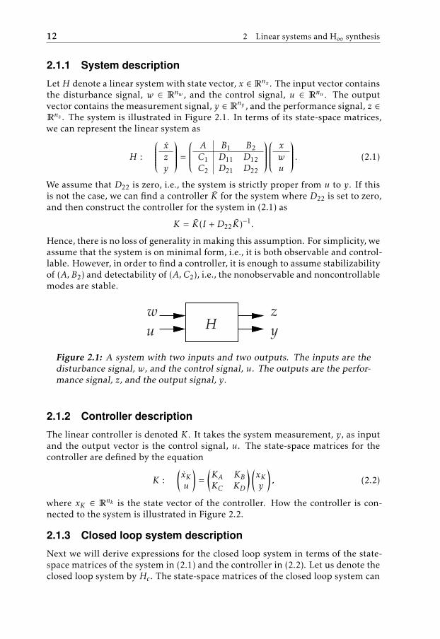
Let H denote a linear system with state vector, x ∈ Rnx . The input vector containsthe disturbance signal, w ∈ Rnw , and the control signal, u ∈ Rnu . The outputvector contains the measurement signal, y ∈ Rny , and the performance signal, z ∈Rnz . The system is illustrated in Figure 2.1. In terms of its state-space matrices,
we can represent the linear system as
H :
xzy
=
A B1 B2C1 D11 D12C2 D21 D22
xwu
. (2.1)
We assume that D22 is zero, i.e., the system is strictly proper from u to y. If thisis not the case, we can find a controller K for the system where D22 is set to zero,and then construct the controller for the system in (2.1) as
K = K(I + D22K)−1.
Hence, there is no loss of generality in making this assumption. For simplicity, weassume that the system is on minimal form, i.e., it is both observable and control-lable. However, in order to find a controller, it is enough to assume stabilizabilityof (A, B2) and detectability of (A, C2), i.e., the nonobservable and noncontrollablemodes are stable.
Hw
u
z
y
Figure 2.1: A system with two inputs and two outputs. The inputs are thedisturbance signal, w, and the control signal, u. The outputs are the perfor-mance signal, z, and the output signal, y.
2.1.2 Controller description
The linear controller is denoted K . It takes the system measurement, y, as inputand the output vector is the control signal, u. The state-space matrices for thecontroller are defined by the equation
K :(xKu
)=
(KA KBKC KD
) (xKy
), (2.2)
where xK ∈ Rnk is the state vector of the controller. How the controller is con-nected to the system is illustrated in Figure 2.2.
2.1.3 Closed loop system description
Next we will derive expressions for the closed loop system in terms of the state-space matrices of the system in (2.1) and the controller in (2.2). Let us denote theclosed loop system by Hc. The state-space matrices of the closed loop system can

2.2 The H∞ norm 13
H
K
w
yu
z
Figure 2.2: A standard setup for H∞ controller synthesis, with the system Hcontrolled through feedback by the controller K .
be derived by combining (2.1) and (2.2) to obtain the following.
u = KCxK + KDy = KCxK + KDC2x + KDD21w
xK = KAxK + KBy = KAxK + KBC2x + KBD21w
x = Ax + B1w + B2u = (A + B2KDC2)x + B2KCxK + (B1 + B2KDD21)w
z = C1x + D11w + D12u
= (C1 + D12KDC2)x + D12KCxK + (D11 + D12KDD21)w
From the equations above we obtain the closed loop expression as
Hc :
xxKz
=
A + B2KDC2 B2KC B1 + B2KDD21KBC2 KA KBD21
C1 + D12KDC2 D12KC D11 + D12KDD21
xxKw
. (2.3)
Denoting the closed loop system states xC =(xxK
)and using the above matrix
partitioning, we can write (2.3) as
Hc :(xCz
)=
(AC BCCC DC
) (xCw
), (2.4)
where xC ∈ Rnx+nk . Using the system matrices in (2.4) we can write the transferfunction of Hc in terms of its system matrices AC , BC , CC , DC as
Hc(s) = CC(sI − AC)−1BC + DC . (2.5)
2.2 The H∞ norm
In this section we introduce the concept of H∞ norm and conditions in terms oflinear matrix inequalities (LMIs) of its upper bound. First, we define the follow-ing.
Definition 2.1 (H∞ norm of a system). Let the transfer function of a stable lin-ear system be given byH(s) = C(sI−A)−1B+D, where A, B, C, D are its state-space
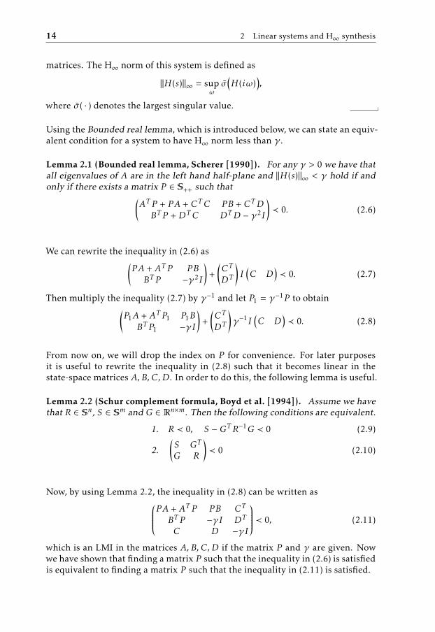
14 2 Linear systems and H∞ synthesis
matrices. The H∞ norm of this system is defined as
‖H(s)‖∞ = supωσ(H(iω)
),
where σ ( · ) denotes the largest singular value.
Using the Bounded real lemma, which is introduced below, we can state an equiv-alent condition for a system to have H∞ norm less than γ .
Lemma 2.1 (Bounded real lemma, Scherer [1990]). For any γ > 0 we have thatall eigenvalues of A are in the left hand half-plane and ‖H(s)‖∞ < γ hold if andonly if there exists a matrix P ∈ S++ such that(
AT P + P A + CT C P B + CTDBT P + DT C DTD − γ2I
)≺ 0. (2.6)
We can rewrite the inequality in (2.6) as(P A + AT P P BBT P −γ2I
)+
(CT
DT
)I(C D
)≺ 0. (2.7)
Then multiply the inequality (2.7) by γ−1 and let P1 = γ−1P to obtain(P1A + AT P1 P1B
BT P1 −γI
)+
(CT
DT
)γ−1I
(C D
)≺ 0. (2.8)
From now on, we will drop the index on P for convenience. For later purposesit is useful to rewrite the inequality in (2.8) such that it becomes linear in thestate-space matrices A, B, C, D. In order to do this, the following lemma is useful.
Lemma 2.2 (Schur complement formula, Boyd et al. [1994]). Assume we havethat R ∈ Sn, S ∈ Sm and G ∈ Rn×m. Then the following conditions are equivalent.
1. R ≺ 0, S − GT R−1G ≺ 0 (2.9)
2.(S GT
G R
)≺ 0 (2.10)
Now, by using Lemma 2.2, the inequality in (2.8) can be written asP A + AT P P B CT
BT P −γI DT
C D −γI
≺ 0, (2.11)
which is an LMI in the matrices A, B, C, D if the matrix P and γ are given. Nowwe have shown that finding a matrix P such that the inequality in (2.6) is satisfiedis equivalent to finding a matrix P such that the inequality in (2.11) is satisfied.
2.3 H∞ controller synthesis 15
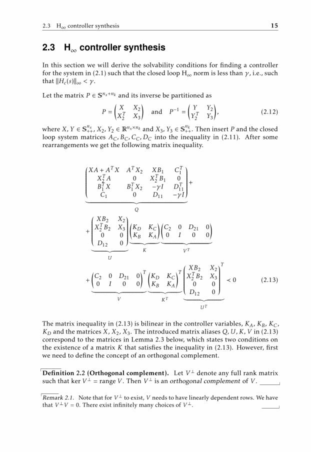
2.3 H∞ controller synthesis
In this section we will derive the solvability conditions for finding a controllerfor the system in (2.1) such that the closed loop H∞ norm is less than γ , i.e., suchthat ‖Hc(s)‖∞ < γ .
Let the matrix P ∈ Snx+nk and its inverse be partitioned as
P =(X X2XT2 X3
)and P −1 =
(Y Y2Y T2 Y3
), (2.12)
where X, Y ∈ Snx++, X2, Y2 ∈ Rnx×nk and X3, Y3 ∈ Snk++. Then insert P and the closed
loop system matrices AC , BC , CC , DC into the inequality in (2.11). After somerearrangements we get the following matrix inequality.
XA + ATX ATX2 XB1 CT1XT2 A 0 XT2 B1 0BT1 X BT1 X2 −γI DT
11C1 0 D11 −γI
︸ ︷︷ ︸Q
+
+
XB2 X2XT2 B2 X3
0 0D12 0
︸ ︷︷ ︸U
(KD KCKB KA
)︸ ︷︷ ︸
K
(C2 0 D21 00 I 0 0
)︸ ︷︷ ︸
V T
+(C2 0 D21 00 I 0 0
)T︸ ︷︷ ︸
V
(KD KCKB KA
)T︸ ︷︷ ︸
KT
XB2 X2XT2 B2 X3
0 0D12 0
T
︸ ︷︷ ︸UT
≺ 0 (2.13)
The matrix inequality in (2.13) is bilinear in the controller variables, KA, KB, KC ,KD and the matrices X, X2, X3. The introduced matrix aliases Q,U, K, V in (2.13)correspond to the matrices in Lemma 2.3 below, which states two conditions onthe existence of a matrix K that satisfies the inequality in (2.13). However, firstwe need to define the concept of an orthogonal complement.
Definition 2.2 (Orthogonal complement). Let V ⊥ denote any full rank matrixsuch that kerV ⊥ = rangeV . Then V ⊥ is an orthogonal complement of V .
Remark 2.1. Note that for V⊥ to exist, V needs to have linearly dependent rows. We havethat V⊥V = 0. There exist infinitely many choices of V⊥.

16 2 Linear systems and H∞ synthesis
Lemma 2.3 (Elimination lemma, Gahinet and Apkarian [1994]). Given matri-ces Q ∈ Sn, U ∈ Rn×m, V ∈ Rn×p, there exists a K ∈ Rm×p such that
Q + UKV T + V KTU T ≺ 0, (2.14)
if and only if
U⊥QU⊥T ≺ 0 and V ⊥QV ⊥T ≺ 0, (2.15)
where U⊥ is an orthogonal complement of U and V ⊥ is an orthogonal comple-ment of V . If U⊥ or V ⊥ does not exist, the corresponding inequality disappears.
In order to apply Lemma 2.3 to the inequality in (2.13), we need to derive theorthogonal complements U⊥ and V ⊥. Note that U in (2.13) can be factorized as
U =
XB2 X2XT2 B2 X3
0 0D12 0
=(P 00 I
) B2 00 I0 0D12 0
.and an orthogonal complement U⊥ can now be constructed as
U⊥ =
B2 00 I0 0D21 0
⊥ (
P −1 00 I
).
By using Lemma 2.3 and performing some rearrangements, the inequality (2.13)is now equivalent to the two LMIs(
NX 00 I
)T XA + ATX XB1 CT1BT1 X −γI DT
11C1 D11 −γI
(NX 00 I
)≺ 0
(NY 00 I
)T AY + YAT YCT1 B1C1Y −γI D11BT1 DT
11 −γI
(NY 00 I
)≺ 0,
(2.16)
where NX and NY denote any bases of the nullspaces of(C2 D21
)and
(BT2 DT12
)respectively. Now, the LMIs in (2.16) are coupled by the relation of X and Ythrough (2.12), which can be simplified after using the following lemma.
Lemma 2.4 (Packard [1994]). Suppose X, Y ∈ Snx++ and nk being a nonnegativeinteger. Then the following statements are equivalent.
1. There exist X2, Y2 ∈ Rnx×nk and X3, Y3 ∈ Rnk such that
P =(X X2XT2 X3
)� 0 and P −1 =
(Y Y2Y T2 Y3
)� 0. (2.17)
2.3 H∞ controller synthesis 17
2. The following inequalities hold.(X II Y
)� 0 and rank
(X II Y
)≤ nx + nk . (2.18)
Remark 2.2. Note that the first inequality in (2.18) implies that Y � 0. The factorization(X II Y
)=
(I Y −1
0 I
) (X − Y −1 0
0 Y
) (I 0Y −1 I
)(2.19)
implies that
rank(X II Y
)= rank(X − Y −1) + rank(Y ) = rank(XY − I) + nx.
Using this fact, the second inequality in (2.18) is equivalent to
rank(XY − I) ≤ nk . (2.20)
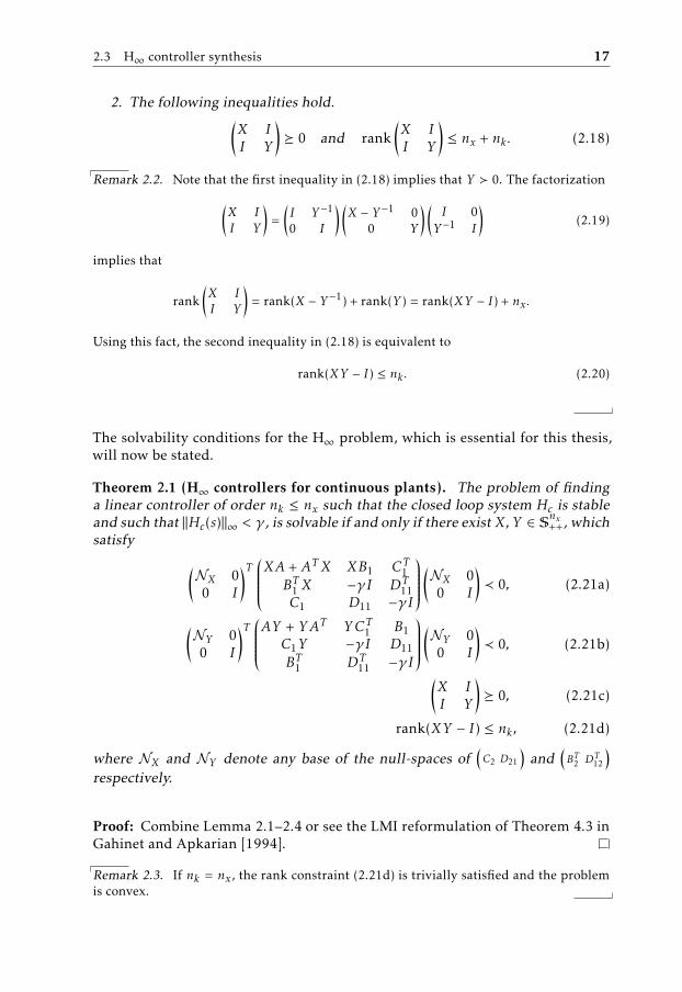
The solvability conditions for the H∞ problem, which is essential for this thesis,will now be stated.
Theorem 2.1 (H∞ controllers for continuous plants). The problem of findinga linear controller of order nk ≤ nx such that the closed loop system Hc is stableand such that ‖Hc(s)‖∞ < γ , is solvable if and only if there exist X, Y ∈ Snx++, whichsatisfy (
NX 00 I
)T XA + ATX XB1 CT1BT1 X −γI DT
11C1 D11 −γI
(NX 00 I
)≺ 0, (2.21a)
(NY 00 I
)T AY + YAT YCT1 B1C1Y −γI D11BT1 DT
11 −γI
(NY 00 I
)≺ 0, (2.21b)
(X II Y
)� 0, (2.21c)
rank(XY − I) ≤ nk , (2.21d)
where NX and NY denote any base of the null-spaces of(C2 D21
)and
(BT2 DT12
)respectively.
Proof: Combine Lemma 2.1–2.4 or see the LMI reformulation of Theorem 4.3 inGahinet and Apkarian [1994].
Remark 2.3. If nk = nx, the rank constraint (2.21d) is trivially satisfied and the problemis convex.

18 2 Linear systems and H∞ synthesis
2.4 Gramians and balanced realizations
It is well known that for a linear system, there exist infinitely many realizationsand for two realizations of the same system, there exists a nonsingular transfor-mation matrix T that connects the representations. Let A, B, C, D and A, B, C, Dbe the system matrices for two realizations of the same system. Then there exista nonsingular transformation matrix T such that
A = T AT −1, B = T B, C = CT −1, D = D. (2.22)
The two systems have the same input-output properties, but are represented dif-ferently. The state vectors are connected by the relation x = T x.
Definition 2.3 (Controllability and observability gramians). Let A, B, C, D bethe system matrices for a stable linear system H of order nx. Then there existX, Y ∈ Snx++ that satisfy
XA + ATX + BBT = 0, AY + YAT + CT C = 0, (2.23)
where X and Y are called the controllability and observability gramians, respec-tively.
The gramians are often used in model reduction algorithms and can be inter-preted as a measure of controllability and observability of a system. For moredetails, see e.g. Glover [1984] or Skogestad and Postlethwaite [1996].
Definition 2.4 (Balanced realization). A system is said to be in a balanced re-alization if the controllability and observability gramians are equal and diago-nal matrices, i.e., X = Y = Σ, where Σ = diag(σ1, . . . , σn). The diagonal entries{σ1, . . . , σn} are called the Hankel singular values.
For any stable linear system, a transformation matrix T can be computed thatbrings the system to a balanced realization by using (2.22). The procedure isdescribed in e.g. Glover [1984], and is stated in Algorithm 1 for convenience.
Actually, we can perform a more general type of a balanced realization aroundany X0, Y0 ∈ S
nx++ which is described in Definition 2.5.
Definition 2.5 (Balanced realization around X0,Y0). Given any X0, Y0 ∈ Snx++
which need not necessarily be solutions to (2.23), it is possible to calculate a trans-formation T such that (2.25) holds. Then the realization described by (2.24) is aBalanced realization around X0, Y0.
The balancing procedure around X0, Y0 is the same as normal balancing, thusAlgorithm 1 can be used for the same purpose.

2.5 Recovering the matrix P from X and Y 19
Algorithm 1 Transforming a system into a balanced realization, Glover [1984]
Assume that the matrices X, Y ∈ Snx++ and the system matrices A, B, C, D are
given.1: Perform a Cholesky factorization of X and Y such that
X = RTXRX and Y = RTYRY .
2: Then perform a singular value decomposition (SVD) such that
RYRTX = UΣV T ,
where Σ is a diagonal matrix with the singular values along the diagonal.
3: The state transformation can now be calculated as
T = Σ−1/2V T RX .
4: The system matrices for a balanced realization of the system are given by
A = T AT −1, B = T B, C = CT −1, D = D. (2.24)
The controllability gramian and observability gramian are given by
X = T −TXT −1 = Σ, Y = T Y T T = Σ. (2.25)
2.5 Recovering the matrix P from X and Y
Assume that we have found X, Y ∈ Snx++ that satisfy (2.21). We now wish to con-struct a P such that (2.17) holds. First note the equality
P −1 =(Y Y2Y T2 Y3
)=
((X − X2X
−13 XT2 )−1 −X−1X2(X3 − XT2 X−1X2)−1
−X−13 XT2 (X − X2X
−13 XT2 )−1 (X3 − XT2 X−1X2)−1
),
(2.26)
which is verified by multiplying the expression in (2.26) by the matrix
P =(X X2XT2 X3
)from the left. Using the fact that the (1, 1) elements in (2.26) are equal, the fol-lowing equality must hold.
X − Y −1 = X2X−13 XT2 (2.27)
Now we intend to find X2 ∈ Rnx×nk and X3 ∈ Rnk×nk that satisfy the equality in(2.27). Perform a Cholesky factorization of X and Y such that X = RTXRX andY = RTYRY . Then we have that
RTXRX − R−1Y R
−TY = X2X
−13 XT2 ,

20 2 Linear systems and H∞ synthesis
which after multiplication by RY from the left and by RTY from the right becomes
RYRTXRXR
TY − I = RYX2X
−13 XT2 R
TY .
Then use a singular value decomposition RYRTX = UΣV T to obtain
U (Σ2 − I)U T = U Γ 2U T = RYX2X−13 XT2 R
TY , (2.28)
where
Σ =(Σnk 00 Inx−nk
), Γ 2 = Σ2 − Inx and Γ =
(Γnk 00 0
).
Let the transformation matrix be T = Σ−1/2V T RX which balances the system, i.e.,we have that T −TXT −1 = T Y T T = Σ. Now we can choose
X3 = Σnk and X2 = T T(Γnk0
),
which satisfy (2.17) and (2.28).
2.6 Obtaining the controller
In the previous section we recovered the matrix variable P . The controller state-space matrices KA, KB, KC , KD can be obtained by solving the following convexoptimization problem, which was suggested in Beran [1997].
minimized,KA,KB,KC ,KD
d
subject to F(P ) ≺ dI(2.29)
Where F(P ) is defined as the left hand side of the matrix inequality in (2.13).Since we have used Theorem 2.1, we know that the optimal value d∗ of the prob-lem in (2.29) satisfies d∗ < 0 and that the closed loop system has an H∞ norm thatis less than γ , i.e., we have that
‖Hc(s)‖∞ < γ.
2.7 A general algorithm for H∞ synthesis
Now we summarize the contents of this chapter in an algorithm for H∞ synthesisusing an LMI approach in Algorithm 2.
Algorithm 2 Algorithm for H∞ synthesis using LMIsAssume that γ , nk and system matrices A, B, C, D are given.
1: Find X, Y ∈ Snx++ that satisfy (2.21).2: Recover P from X and Y as described in Section 2.5.3: Solve (2.29) to get the controller system matrices KA, KB, KC , KD .

3Optimization
An optimization problem is defined by an objective function and a set of con-straints. The aim is to minimize the objective function while satisfying the con-straints. In this chapter, optimization preliminaries are presented and somemethods that can be used to solve optimization problems are outlined. The pre-sentation closely follows relevant sections in Boyd and Vandenberghe [2004] andNocedal and Wright [2006]. Those familiar with the subject may want to skipdirectly to the next chapter.
3.1 Nonconvex optimization
In a nonconvex optimization problem, the objective function or the feasible setor both are nonconvex. There is no efficient method to solve a general nonconvexoptimization problem, so specialized methods are often used to solve them. It isnot possible in general to predict how difficult it is to solve a nonconvex problemand even small problems with few variables may be hard to solve. Nonconvexoptimization is a very active research topic today.
3.1.1 Local methods
One approach to use when solving nonconvex optimization problems is to use lo-cal methods. A local method searches among the feasible points in a local neigh-borhood for the optimal point. The drawback for this kind of methods is that asolution that is found may not be the global optimum, and that it may be verysensitive to the choice of the starting point, which in general must be provided orfound using some heuristics. There are parameters that may have to be tuned forthese algorithms to work. All methods that are presented in this thesis are localmethods.
21
22 3 Optimization
3.1.2 Global methods
In contrast to local methods, global methods find the global minimum of a non-convex minimization problem. It can be very hard to construct such methodsand they tend to be very complex and time consuming in general, and thus notefficient in practice. This of course does not mean that global methods cannot besuccessful for certain subclasses of nonconvex optimization problems. However,we will not consider or analyze any global methods in this thesis.
3.2 Convex optimization
Convex optimization problems belong to a subgroup of nonlinear optimizationproblems, where both the objective function is convex and the feasible set is con-vex. This in turn gives some very useful properties. A locally optimal point for aconvex optimization problem is the global optimum, see Boyd and Vandenberghe[2004]. Convex problems are in general easy to solve in comparison to nonconvexproblems. However, it may not always be the case due to e.g. large scale issues,numerical issues or both.
3.3 Definitions
In this section we present some definitions and concepts that are commonly usedin optimization and later on in this thesis.
3.3.1 Convex sets and functions
In this section, convex sets and functions are defined, which are important con-cepts in optimization since they imply some very useful properties.
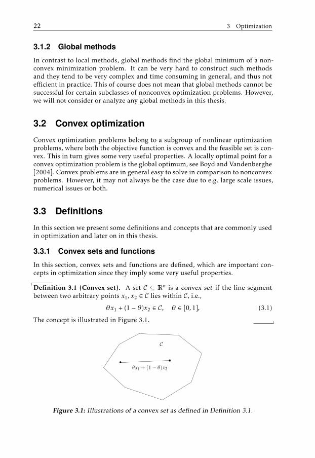
Definition 3.1 (Convex set). A set C ⊆ Rn is a convex set if the line segment
between two arbitrary points x1, x2 ∈ C lies within C, i.e.,
θx1 + (1 − θ)x2 ∈ C, θ ∈ [0, 1], (3.1)
The concept is illustrated in Figure 3.1.
θx1 + (1 − θ)x2
C
Figure 3.1: Illustrations of a convex set as defined in Definition 3.1.

3.3 Definitions 23
With the definition of a convex set, we can continue with the definition of a con-vex function.
Definition 3.2 (Convex function). A function f : Rn → R is a convex functionif dom f is a convex set and if for all x1, x2 ∈ dom f we have that
f(θx1 + (1 − θ)x2
)≤ θf (x1) + (1 − θ)f (x2), θ ∈ [0, 1]. (3.2)
In plain words, this means that the line segment between the points(x1, f (x1)
)and
(x2, f (x2)
)lies above the graph of f as illustrated in Figure 3.2.
(x1, f (x1)
) (x2, f (x2)
)θ f (x1) + (1 − θ) f (x2)
f(θx1 + (1 − θ)x2
)
f
x1 x2
Figure 3.2: Illustrations of a convex function as defined in Definition 3.2.
3.3.2 Cones
In this section we define a special kind of sets, referred to as cones.
Definition 3.3 (Cone). A set K ⊆ Rn is a cone, if for every x ∈ K we have that
θx ∈ K, θ ≥ 0. (3.3)
Definition 3.4 (Convex cone). A cone K ⊆ Rn is a convex cone, if it is convex orequivalently, if for arbitrary points x1, x2 ∈ K we have
θ1x1 + θ2x2 ∈ K, θ1, θ2 ≥ 0. (3.4)
Cones provide the foundation for defining generalized inequalities, but beforewe explain this concept, we first need to define a proper cone.
Definition 3.5 (Proper cone). A convex cone K is a proper cone, if the followingproperties are satisfied:

24 3 Optimization
• K is closed.
• K is solid, i.e., it has nonempty interior.
• K is pointed, i.e., x ∈ K and −x ∈ K implies x = 0.
3.3.3 Generalized inequalities
Definition 3.6 (Generalized inequality). A generalized inequality �K with re-spect to a proper cone K is defined as
x1 �K x2 ⇔ x1 − x2 ∈ K. (3.5)
The strict generalized inequality (�K) is defined analogously. From now on, theindex K is dropped when the cone is implied from context. We remark that theset of positive semidefinite matrices is a proper cone.
Example 3.1Let A be a real symmetric matrix of dimension n × n, i.e., A ∈ Sn. If the propercone K is defined as the set of positive semidefinite matrices, then A � 0 meansthat A lies strictly in the cone K which is equivalent to that all eigenvalues of Aare strictly positive.
Now we define an optimization problem with matrix inequality constraints usingthe concepts described previously in this chapter.
minimizex
f0(x)
subject to fi(x) � 0, i ∈ I ,hi(x) = 0, i ∈ E ,
(3.6)
where f0 : Rn → R, fi : Rn → Smi , hi : Rn → R
mi , and where � denotes positivesemidefiniteness. The functions are smooth and real-valued and E and I are twofinite sets of indices.
3.3.4 Logarithmic barrier function and the central path
Definition 3.7 (Generalized logarithm for Sm+ ). The function
ψ(X) = log detX (3.7)
is a Generalized logarithm for the cone Sm+ with degree m.
The Central path is a concept that emerged as the barrier methods became pop-ular, mostly used in the context of convex optimization. It is also referred to asThe barrier trajectory.

3.4 First order optimality conditions 25
Definition 3.8 (Central path, logarithmic barrier formulation). The Centralpath of the problem (3.6) is the set of points x∗(µ), µ ≥ 0, that solves the followingoptimization problems.
minimizex
f0(x) − µ∑i∈I
ψ(fi(x)).
subject to hi(x) = 0, i ∈ E .(3.8)
This proposes a way to solve (3.6) by iteratively solving (3.8) for a sequence ofvalues µk that approaches zero. The optimal point in iteration k can be used asan initial point in iteration k+1, see e.g. Boyd and Vandenberghe [2004].
Note that the central path might not be unique in case that the problem is notconvex.
3.4 First order optimality conditions
In this section, the first order necessary conditions for x∗ to be a local minimizerare stated. When presenting these conditions, the following definition is useful.
Definition 3.9 (Lagrangian function). The Lagrangian function (or just La-grangian for short) for the problem in (3.6) is
L(x, Z, v) = f0(x) −∑i∈I〈Zi , fi(x)〉 −
∑i∈E〈νi , hi(x)〉 (3.9)
where Zi ∈ Smi+ , νi ∈ Rmi and 〈A, B〉 = trace(AT B) denotes the inner product
between A and B.
Assume that the point x∗ satisfy assumptions about regularity, see e.g. Forsgrenet al. [2002] or Forsgren [2000] for the semidefinite case. We are now ready tostate the first-order necessary conditions for (3.6) that must hold at x∗ for it to bean optimum.
Theorem 3.1 (First order necessary conditions for optimality, Boyd and Van-denberghe [2004]). Suppose x∗ ∈ Rn is any local solution of (3.6), and thatthe functions fi , hi in (3.6) are continuously differentiable. Then there exists La-grange multipliers Z∗i ∈ S
mi , i ∈ I and ν∗i ∈ Rmi , i ∈ E, such that the following
conditions are satisfied at (x∗, Z∗, ν∗)
∇xL(x∗, Z∗, ν∗) = 0, (3.10a)
hi(x∗) = 0, i ∈ E , (3.10b)
fi(x∗) � 0, i ∈ I , (3.10c)
Z∗i fi(x∗) = 0, i ∈ I , (3.10d)
Z∗i � 0, i ∈ I . (3.10e)

26 3 Optimization
The conditions (3.10) are sometimes referred to as the Karush-Kuhn-Tucker con-ditions or the KKT conditions for short. See Karush [1939] or Kuhn and Tucker[1951] for early references.
3.5 Unconstrained optimization
In this section we will present useful background theory for solving the uncon-strained optimization problem
minimizex∈Rn
f (x), (3.11)
where f : Rn → R is twice continuously differentiable. We assume that theproblem has at least one local optimum x∗.
There exist several kinds of methods to solve problems like (3.11), e.g. trust-region methods, line search methods and derivative-free optimization methods,see e.g. Nocedal and Wright [2006], Bertsekas [1995]. We will describe Newton’smethod, which is a line search method. Newton’s method is thoroughly describedin e.g. Nocedal and Wright [2006], Boyd and Vandenberghe [2004], Bertsekas[1995].
The following theorem defines a necessary characteristic for a locally optimalpoint of the unconstrained problem in (3.11).
Theorem 3.2 (First order necessary conditions, Nocedal and Wright [2006]).If x∗ is a local minimizer and f (x) is continuously differentiable in an open neigh-borhood of x∗, then ∇f (x∗) = 0.
3.5.1 Newton’s method
Assume a point xk ∈ dom f (x) is given. Then the second order Taylor approxima-tion (or model) Mk(p) of f (x) at xk is defined as
Mk(p) = f (xk) + ∇f (xk)T p +
12pT∇2f (xk)p. (3.12)
Definition 3.10. The Newton direction pNK is defined by
∇2f (xk)pNk = −∇f (xk). (3.13)
The Newton direction has some interesting properties. If ∇2f (xk) � 0:
• pNk minimizes Mk(p) in (3.12), as illustrated in Figure 3.3.
• ∇f (xk)T pNk = −∇f (xk)T
(∇2f (xk)
)−1∇f (xk) < 0 unless ∇f (xk) = 0, i.e., the
Newton step is a descent direction unless xk is a local optimum.

3.5 Unconstrained optimization 27
(xk, f (xk)
)Mk(p)
f (x)
f (x)(xk + pN
k , f (xk + pNk )
)(
x∗, f (x∗))
x
Figure 3.3: The function f (x) and its second order Taylor approximationMk(p). The Newton step pNk is the minimizer of Mk(p). The optimum x∗
minimizes f (x).
If ∇2f (xk) � 0, the Newton step does not minimize Mk(p) and is not guaran-teed be a descent direction. If that is the case, let Bk be a positive definite ap-proximation of ∇2f (x), i.e. Bk ∈ S++, and choose the search direction by solvingBkp
Mk = −∇f (xk). Then pMk is guaranteed to be a descent direction and minimizes
the convex quadratic model
MBk (p) = f (xk) + ∇f (xk)
T p +12pT Bkp. (3.14)
Some methods to obtain approximations Bk ∈ S++ of the Hessian will be pre-sented in Section 3.5.3.
Definition 3.11 (Newton decrement). The Newton decrement Λ(xk) is definedas
Λ(xk) =(∇f (xk)
T B−1k ∇f (xk)
)1/2= (−∇f (xk)
T pMk )1/2. (3.15)
The Newton decrement is useful as a stopping criterion. Let MBk (p) be the convex
quadratic model of f at xk . Then
f (xk) − infpMBk (p) = f (xk) −MB
k (pMk ) =12Λ(xk)
2, (3.16)
and we see that Λ(xk)2/2 can be interpreted as an approximation of f (xk)−p∗, i.e.,a measure of distance from optimality based on the modified quadratic convexapproximation of f at xk .

28 3 Optimization
3.5.2 Line search
When a descent direction pMk is determined, we want to find the minimum of thefunction along that direction. Since MB
k (p) is only an approximation, pMk will notnecessarily minimize f (xk+p). The problem of minimizing the objective functionalong the search direction can be stated as
minimizeα∈(0,1]
f (xk + αpMk ), (3.17)
which is called exact line search. An approximate method, but cheaper in compu-tation than exact line search, is Backtracking line search. The idea is not to solve(3.17) exactly, but just to reduce f enough, according to some criterion. The pro-cedure is outlined in Algorithm 3 and illustrated in Figure 3.4.
α = 0 α0
f (xk) + α∇ f (xk)T pk
f (xk) + αβ∇ f (xk)T pk
f (xk + αpk)
α
f
Figure 3.4: The figure illustrates Backtracking line search. The curve showsthe function f along the descent direction. The lower dashed line shows thelinear extrapolation of f and the upper dashed line has a slope of factor βsmaller. The condition for accepting a point is that α ≤ α0.
Algorithm 3 Backtracking line search
Given a descent direction pk for f (xk), β ∈ (0, 0.5), γ ∈ (0, 1).α := 1while f (xk + αpk) > f (xk) + βα∇f (xk)T doα := γα
end while

3.5 Unconstrained optimization 29
3.5.3 Hessian modifications
As mentioned in Section 3.5.1, it is important that the Hessian approximation Bkin (3.14) is positive definite for the calculated step to be a descent direction. Thereare several ways to modify the Hessian in order to achieve this. The main idea isto make the smallest modification possible in order not to change the curvaturemore than necessary. We will describe some of these methods in this section.
Eigenvalue computation
A straight-forward approach would be to calculate the eigenvalues of the Hessian∇2f (x) and choose the approximation to be
B = ∇2f (xk) + dI � 0, d ≥ 0, (3.18)
where d > λmin
(∇2f (xk)
).
Cholesky factorization
Another suggestion would be to try and calculate the Cholesky factors R of (3.18),
RT R = ∇2f (xk) + dI � 0, (3.19)
starting with d = 0 and successively trying greater values until we succeed. Thiswill guarantee (with quite high accuracy) that RT R > 0 since Cholesky factoriza-tion can only be carried out on a positive definite matrix. The disadvantage ofthis method is that we do not beforehand know which d that is appropriate, andtherefore we might have to make many tries before we succeed. A similar butsomewhat more elaborate procedure is described in [Nocedal and Wright, 2006,Appendix B].
Modified symmetric indefinite factorization
For any symmetric matrix B it is possible to calculate the factorization
P T BP = LDLT , (3.20)
which is called the symmetric indefinite factorization or LDL factorization, seee.g. Golub and Van Loan [1996]. The matrix L is a lower triangular matrix, Pis a permutation matrix and D is a block diagonal matrix with block sizes of1 × 1 and 2 × 2, which makes it tridiagonal. A procedure that is presented inCheng and Higham [1998] is to then calculate a modification matrix F such thatL(D +F)LT is positive definite. In order to calculate this modification matrix, onefirst computes the eigenvalue factorization
D = QDQT , (3.21)
and then calculates the modification matrix
F = QEQT ,

30 3 Optimization
where the diagonal matrix E is defined by
Eii =
0, if Dii ≥ δ,δ − Dii , if Dii < δ,
i = 1, 2, . . . (3.22)
The matrix F is now the minimal matrix in Frobenius norm such that D + F � δI .Note that since D is tridiagonal, calculating the eigenvalue factorization in (3.21)is computationally cheap.
3.5.4 Newton’s method with Hessian modification
Now we outline a method in Algorithm 4, which is based on Algorithm 9.5 inBoyd and Vandenberghe [2004]. The stopping criterion used is the Newton decre-ment, defined in Definition 3.11.
Algorithm 4 Newton’s method with Hessian modification
Given a starting point x0 ∈ dom f , tolerance ε > 0loop
Compute the Newton step by solving BkpMk = −∇f (xk) with approximate
Hessian Bk � 0.Compute the Newton decrement Λ(xk).if Λ(xk) < Λtol then
Exit loop.end ifChoose step size αk by using Backtracking line search.Update iterate. xk+1 := xk + αkp
Mk .
Set k := k + 1.end loop
3.5.5 Quasi-Newton methods
Quasi-Newton methods only require the gradient of the objective function to besupplied at each iteration. By measuring the change in gradient they updatethe Hessian estimate from the previous iterate in a way that is good enough toproduce superlinear convergence.
Especially in cases where the Hessian is unavailable or computationally expen-sive to calculate, quasi-Newton methods are efficient to use. Among the quasi-Newton methods, the BFGS method (named after its discoverers Broyden [1970],Fletcher [1970], Goldfarb [1970], Shanno [1970]) is perhaps the most well-knownand most popular. According to Nocedal and Wright [2006] it is presently con-sidered to be the most effective of all quasi-Newton updating formulae.
BFGS updating
The BFGS updating formulae is derived in a quite intuitive way in Nocedal andWright [2006], where also additional details are given. Below we will brieflysummarize the main ideas in the derivation.

3.5 Unconstrained optimization 31
Suppose we have formed the convex quadratic approximate model of the objec-tive function as in (3.14). The minimizer of the convex quadratic model MB
k (p)can be written explicitly as
pk = −B−1k ∇fk
and is used as the search direction to update the iterate as
xk+1 = xk + αpk .
where the step length α is chosen in a way such that it satisfies the Wolfe condi-tions, see Nocedal and Wright [2006]. Define the vectors
sk = xk+1 − xk , yk = ∇fk+1 − ∇fk . (3.23)
and let the inverse of Bk be denoted Hk . By requiring that ∇pMBk (sk) = ∇fk+1 in
(3.14) we get that
Hk+1yk = sk , (3.24)
which is usually referred to as the secant equation. Since we require that Hk+1 ∈S++, the equation (3.24) is feasible only if yk and sk satisfy the curvature condi-tion,
yTk sk > 0, (3.25)
which follows from multiplying (3.24) by yTk . The inverse Hessian update Hk+1is now obtained as the minimizer to the following optimization problem.
minimizeH
‖H − Hk‖W
subject to Hyk = sk , H ∈ S++
(3.26)
where W is any matrix satisfying Wsk = yk and ‖A‖W = ‖W 1/2AW 1/2‖F is theweighted Frobenius norm. The objective function in (3.26) reflects the desirethat the updated (inverse) Hessian should in some sense be close to the (inverse)Hessian in the previous iteration. The unique solution to (3.26) is given by
Hk+1 =(I −
skyTk
yTk sk
)Hk
(I −
yksTk
yTk sk
)+sks
Tk
yTk sk(3.27)
and by applying the Sherman-Morrison-Woodbury formula (see e.g. [Nocedaland Wright, 2006, Appendix A]) on (3.27) we obtain
Bk+1 = Bk −Bksks
Tk Bk
sTk Bksk+yky
Tk
yTk sk(3.28)
which is the formula that probably is the most known and used for BFGS updat-ing. Other references on BFGS are e.g. the books by Fletcher [1987] and Dennis,Jr. and Schnabel [1983], where the second book of the two also describes an up-date of the Cholesky factor of Bk .

32 3 Optimization
Damped BFGS updating
The curvature condition (3.25) will not always hold for nonconvex functions f (x)or if we do not choose step sizes according to the Wolfe conditions. In those casesone can modify the BFGS update by modifying the definition of yk . Below wewill briefly describe this modified procedure which is known as damped BFGSupdating, which is described in [Nocedal and Wright, 2006, Procedure 18.2].
Given the symmetric and positive definite matrix Bk , define sk and yk as in (3.23)and let
rk = θkyk + (1 − θk)Bksk , (3.29)
where θ is defined as follows.
θk =
1 if sTk yk ≥ 0.2sTk Bksk ,(0.8sTk Bksk)/(s
Tk Bksk − s
Tk yk) if sTk yk < 0.2sTk Bksk
(3.30)
Then obtain the updated Hessian estimate Bk+1 using the formula
Bk+1 = Bk −Bksks
Tk Bk
sTk Bksk+rkr
Tk
rTk sk, (3.31)
which is similar to (3.28) but with yk replaced by rk . This guarantees that Bk+1 ispositive definite and one can verify, using the equations above, that when θk , 1we have
sTk rk = 0.2sTk Bksk > 0. (3.32)
3.6 Constrained optimization
We now turn to constrained optimization. The approach we will present hereis the primal-dual approach. As the name suggests, the approach uses both theoriginal primal variables as well as dual variables. One way to derive this ap-proach is to start from the KKT conditions (3.10) and add slack variables Si tothe inequalities. We get the following equations
∇xL(x∗, Z∗, ν∗) = 0, (3.33a)
hi(x∗) = 0, i ∈ E , (3.33b)
fi(x∗) − S∗i = 0, i ∈ I , (3.33c)
Z∗i S∗i = 0, i ∈ I . (3.33d)
Z∗i � 0, S∗i � 0, i ∈ I , (3.33e)
and we note that this is now a collection of equality constraints, except for theinequality constraints (3.33e). Below we will describe a method for finding asolution to a system of equations.

3.6 Constrained optimization 33
3.6.1 Newton’s method for nonlinear equations
Recall from Section 3.5 that Newton’s method is based on the principle of mini-mizing a second order model, which is created by taking the first three terms ofthe Taylor series approximation, see (3.12), of the function around the current it-erate xk . The Newton step is the vector that minimizes that model. When solvingnonlinear equations, Newton’s method is derived in a similar way, the differenceis that a linear model is used.
Assume that r : Rn → Rn and that we want to find x∗ such that r(x∗) = 0. Assume
we have a point xk such that r(xk) ≈ 0. Denote the Jacobian of r as J(x) and wecan create a linear model Mk(p) of r(xk + p) as
Mk(p) = r(xk) + J(xk)p. (3.34)
If we choose pk = −J(xk)−1r(xk) we see that Mk(pk) = 0 and this choice of pkis Newton’s method in its pure form. A structured description is given in Algo-rithm 5.
Algorithm 5 Newton’s method for nonlinear equations
Given x0for k = 0, 1, 2, . . . do
Calculate a solution pk to the Newton equations J(xk)pk = −r(xk).xk+1 := xk + pk
end for
If any positivity constraints are present, such as (3.33e), we can use line searchtechniques to find a feasible point along the search direction.
Remark 3.1. Note that Newton’s method for nonlinear equations can be extended to func-tions r : Sn → S
n by applying standard differential calculus for matrices.
Remark 3.2. Note that the domain and range of the function defined by the left handside of (3.33) are not the same spaces, since the product in (3.33d) is not symmetric ingeneral. This means that Newton’s method is not directly applicable. A solution is toapply a symmetry transformation to the left hand side in (3.33d) before Newton’s methodis applied. We will come back to this issue in Section 6.4.2.
3.6.2 Central path
With Remark 3.2 in mind, the KKT system in (3.33) can be solved by applyingNewton’s method for equations while ignoring the inequality in (3.33e). However,the inequality in (3.33e) should be taken into consideration when computing thestep length. Unfortunately, due to (3.33d), only very short steps can be taken. Asa result the convergence will be very slow. In order to be able to take longer steps,we can relax the condition in (3.33d). A way to do this relaxation is to use thecentral path.

34 3 Optimization
Definition 3.12 (Central path, primal-dual formulation). The central path isdefined as the set of solution points, parameterized by µ, for which
∇xL(x, Z, ν) = 0, (3.35a)
hi(x) = 0, i ∈ E , (3.35b)
fi(x) − Si = 0, i ∈ I , (3.35c)
ZiSi = µIni , i ∈ I . (3.35d)
Zi � 0, Si � 0, i ∈ I , (3.35e)
where µ ≥ 0 and where L(x, Z, ν) is defined in Definition 3.9.
The idea is to start with a µ = µ0 and let µ tend to zero, in order to make the limitsolution satisfy the KKT conditions. Methods following this principle are calledpath-following methods.
Example 3.2Consider the convex optimization problem
minimizex
cT x
subject to F(x) = F0 +m∑i=1
xiFi � 0(3.36)
where c, x ∈ Rn and Fi ∈ Sn+,∀i. Assume that (3.36) is strictly feasible. Using Defi-nition 3.12, the central path for (3.36) is the set of solution points, parameterizedby µ, for which
∇xL(x, Z)i = ci − trace(ZFi) = 0, ∀iF(x) − S = 0,
ZS = µI,
Z � 0, S � 0,
(3.37)
where Z, S ∈ Sn. If we now instead use Definition 3.8, the central path of (3.36)is the set of solution points x∗(µ) that solves
minimizex
cT x − µ log det F(x). (3.38)
Since (3.38) is a convex problem, by using Theorem 3.1 or Theorem 3.2 we knowthat global minimizers satisfy
ci − µ trace(F−1(x)Fi) = 0, ∀i,F(x) � 0.
(3.39)
By introducing a slack variable S � 0 and defining the dual variable Z = µF−1(x),we actually obtain exactly the same equations as in (3.37) which shows that thetwo definitions coincide for the problem in (3.36).
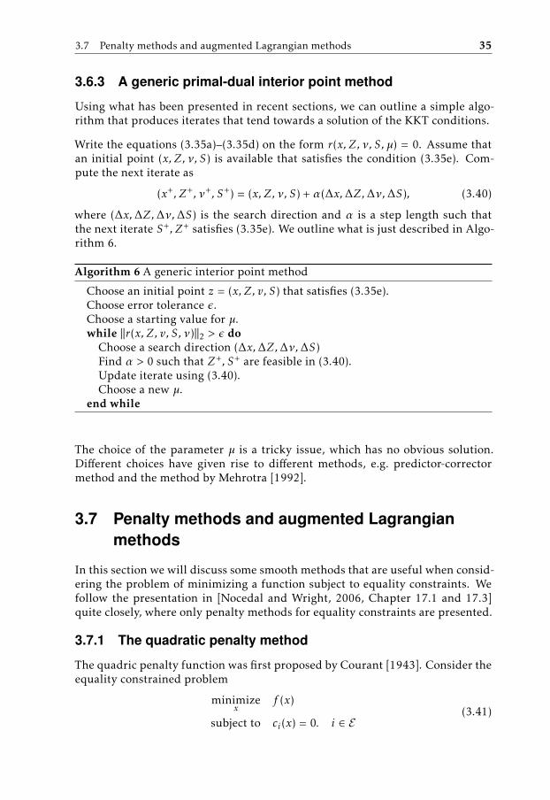
3.7 Penalty methods and augmented Lagrangian methods 35
3.6.3 A generic primal-dual interior point method
Using what has been presented in recent sections, we can outline a simple algo-rithm that produces iterates that tend towards a solution of the KKT conditions.
Write the equations (3.35a)–(3.35d) on the form r(x, Z, ν, S, µ) = 0. Assume thatan initial point (x, Z, ν, S) is available that satisfies the condition (3.35e). Com-pute the next iterate as
(x+, Z+, ν+, S+) = (x, Z, ν, S) + α(∆x,∆Z,∆ν,∆S), (3.40)
where (∆x,∆Z,∆ν,∆S) is the search direction and α is a step length such thatthe next iterate S+, Z+ satisfies (3.35e). We outline what is just described in Algo-rithm 6.
Algorithm 6 A generic interior point method
Choose an initial point z = (x, Z, v, S) that satisfies (3.35e).Choose error tolerance ε.Choose a starting value for µ.while ||r(x, Z, v, S, ν)||2 > ε do
Choose a search direction (∆x,∆Z,∆ν,∆S)Find α > 0 such that Z+, S+ are feasible in (3.40).Update iterate using (3.40).Choose a new µ.
end while
The choice of the parameter µ is a tricky issue, which has no obvious solution.Different choices have given rise to different methods, e.g. predictor-correctormethod and the method by Mehrotra [1992].
3.7 Penalty methods and augmented Lagrangianmethods
In this section we will discuss some smooth methods that are useful when consid-ering the problem of minimizing a function subject to equality constraints. Wefollow the presentation in [Nocedal and Wright, 2006, Chapter 17.1 and 17.3]quite closely, where only penalty methods for equality constraints are presented.
3.7.1 The quadratic penalty method
The quadric penalty function was first proposed by Courant [1943]. Consider theequality constrained problem
minimizex
f (x)
subject to ci(x) = 0. i ∈ E(3.41)

36 3 Optimization
We can formulate a related problem by using a quadratic penalty function as in
minimizex
f (x) +µ
2
∑i∈E
c2i (x), (3.42)
where µ is a the penalty parameter. By squaring the equality constraint violationsand scaling them by µ/2, the minimizer of (3.42) will tend towards being a feasi-ble solution of (3.41) as µ → ∞. An approach would be to consider a sequenceof increasing values {µk} as k → ∞ and for each value of µk , solve (3.42) usingunconstrained optimization. Each solution xk obtained using µk would serve as agood starting point for the following minimization problem when searching forthe minimizer µk+1. If µk → ∞ as k → ∞ it can be proved that every limit pointx∗ of the sequence {xk} is a global solution of the problem (3.41), see [Nocedaland Wright, 2006, Theorem 17.1].
3.7.2 The augmented Lagrangian method
Sometimes also referred to as the method of multipliers, the augmented Lagrang-ian method was proposed independently by Hestenes [1969] and Powell [1969].They were considering an equality constrained optimization problem and it wasshown that the numerical properties were improved compared to using regularpenalty methods, e.g. the one presented in Section 3.7.1. More details regardingmultiplier and penalty methods can be found in the books by Bertsekas [1982,1995], Fletcher [1987], Nocedal and Wright [2006] and the survey paper by Rock-afellar [1993].
Motivation and definition
When using quadratic penalty methods, the minimizers of the problem (3.42)do not quite satisfy the equality constraints of (3.41) unless in the limit whereµk →∞. The augmented Lagrangian method was shown to produce approximateminimizers that more closely satisfy the equality constraints in (3.41), even formoderate values of the penalty parameters µk .
The augmented Lagrangian for the optimization problem (3.41) is defined as
LA(x, λ, µ) = f (x) +∑i∈E
λici(x) +µ
2
∑i∈E
c2i (x), (3.43)
where λi is an estimate the of Lagrange multiplier. We can see that the augmentedLagrangian (3.43) differs from the quadratic penalty function by including a sumof λici(x).
Algorithmic framework
If xk is the approximate minimizer of LA(x, λk , µk) then by the optimality condi-tions for unconstrained minimization, Theorem 3.2, we have that
∇xLA(x, λ) = ∇xf (x) +∑i∈E
(λki + µkci(x)
)∇ci(x) ≈ 0, (3.44)

3.7 Penalty methods and augmented Lagrangian methods 37
which we can compare to the first optimality condition for constrained optimiza-tion, Theorem 3.1, for (3.41) which is
∇xL(x, λ) = ∇xf (x) +∑i∈E
λi∇ci(x) ≈ 0. (3.45)
where we can draw the conclusion that at the optimum xk of (3.43), we have that
λi ≈ λki + µkci(xk), ∀i ∈ E . (3.46)
This suggests an updating rule for the Lagrange multiplier estimates
λk+1i = λki + µkci(xk), ∀i ∈ E . (3.47)
We will now summarize the ideas from this section in Algorithm 7, see also [No-cedal and Wright, 2006, Framework 17.3].
Algorithm 7 An augmented Lagrangian method for equality constraints
Choose µ0 > 0, tolerance τ0 > 0, starting point xs0 and λ0.for k = 0, 1, 2, . . . do
Start at xsk and minimize LA(x, λk , µk) approximately to find xk such that‖∇xLA(xk , λk , µk)‖ ≤ τk .if some convergence test for (3.41) is satisfied then
Stop with approximate solution xk .end ifCalculate the updated Lagrange multipliers λk+1 using (3.47).Choose new penalty parameter µk+1 ≥ µk .Let the starting point for the next iteration be xsk+1 = xk .Set tolerance for next iteration, τk+1.
end for
This completes the chapter of optimization preliminaries.


4The characteristic polynomial and
rank constraints
The approach to low order H∞ control in this thesis involves the characteristicpolynomial of the matrix I − XY in (2.21d). In this chapter we will explain howthe rank constraint of a matrix can be expressed as a quotient of coefficients ofits characteristic polynomial. As a consequence this enables gradient methods tobe applied to the resulting smooth optimization problem. The reference on thistopic is Helmersson [2009].
The chapter is structured as follows. We begin in Section 4.1 by presenting twolemmas regarding properties of the coefficients of the characteristic polynomial.In Section 4.2 we present a modified version of Theorem 2.1, and in Section 4.3we will reformulate the solvability conditions of Theorem 2.1 as an optimiza-tion problem. In Section 4.4 we will describe how to compute the coefficientsof the characteristic polynomial of I − XY and their derivatives. The chapter isconcluded by showing how the problem of finding a dynamic controller (i.e., acontroller with nonzero number of states) can be equivalently rewritten as a prob-lem of finding a static controller (i.e., a controller with no states). Additionally,some advantages and disadvantages of using such an approach in the context oflow order H∞ controller synthesis will be discussed.
4.1 A polynomial criterion
The characteristic polynomial of a matrix Z ∈ Rnx×nx is defined by
det(λI − Z) =nx∑i=0
ci(Z)λi , (4.1)
39

40 4 The characteristic polynomial and rank constraints
where the coefficients ci(Z) are polynomial functions of the elements in the ma-trix Z. Then we have that e.g.
cnx (Z) = 1, cnx−1(Z) = − trace(Z) and c0 = (−1)nx det(Z).
Some other nontrivial properties of the coefficients of the characteristic polyno-mial in the case where the matrix Z is positive semidefinite are presented inLemma 4.1 and Lemma 4.2 below.
Lemma 4.1 (Helmersson [2009]). Let Z ∈ Rnx×nx be a matrix with real non-negative eigenvalues, λi(Z) ≥ 0, and let ci(−Z), i = 1, 2, . . . , nx, be the coefficientsof the characteristic polynomial of −Z as defined in (4.1). Then, the followingstatements are equivalent if nk < nx:
1. cnx−nk−1(−Z) = 0,
2. rankZ ≤ nk .
Lemma 4.2 (Helmersson [2009]). Let Z ∈ Rnx×nx be a matrix with real nonneg-ative eigenvalues ordered by λ1(Z) ≥ λ2(Z) ≥ . . . ≥ λnx (Z) ≥ 0 and assume thatcnx−nk (−Z) , 0. Then, for nk < nx, the following relations hold:
1nk + 1
nx∑i=nk+1
λi(Z) ≤cnx−nk−1(−Z)
cnx−nk (−Z)≤
nx∑i=nk+1
λi(Z), (4.2)
or equivalently
cnx−nk−1(−Z)
cnx−nk (−Z)≤
nx∑i=nk+1
λi(Z) ≤ (nk + 1)cnx−nk−1(−Z)
cnx−nk (−Z). (4.3)
Remark 4.1. For future reference, note that the quotient in (4.2) is nonnegative if Z ispositive semidefinite.
From experience, better numeric properties are obtained by using the quotient in(4.2) instead of only the nominator when searching for matrices Z with low rank.Insights on this can be gained from noting that the quotient in (4.2) is boundedboth from above and from below by the sum of eigenvalues of Z that should bezero for rankZ ≤ nk to hold.
4.2 Replacing the rank constraint
Let us define Z = XY − I , where X, Y ∈ Snx . The following corollary can beproved.
Corollary 4.1. Assume that X, Y ∈ Snx satisfy(X II Y
)� 0, or equivalently, XY − I � 0.
Then the following statements are equivalent:
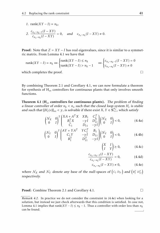
4.2 Replacing the rank constraint 41
1. rank(XY − I) = nk ,
2.cnx−nk−1(I − XY )
cnx−nk (I − XY )= 0, and cnx−nk (I − XY ) , 0.
Proof: Note that Z = XY − I has real eigenvalues, since it is similar to a symmet-ric matrix. From Lemma 4.1 we have that
rank(XY − I) = nk ⇔
rank(XY − I) ≤ nkrank(XY − I) > nk − 1
⇔
cnx−nk−1(I − XY ) = 0cnx−nk (I − XY ) , 0
which completes the proof.
By combining Theorem 2.1 and Corollary 4.1, we can now formulate a theoremfor synthesis of H∞ controllers for continuous plants that only involves smoothfunctions.
Theorem 4.1 (H∞ controllers for continuous plants). The problem of findinga linear controller of order nk < nx such that the closed loop system Hc is stableand such that ‖Hc(s)‖∞ < γ , is solvable if there exist X, Y ∈ Snx++, which satisfy(
NX 00 I
)T XA + ATX XB1 CT1BT1 X −γI DT
11C1 D11 −γI
(NX 00 I
)≺ 0, (4.4a)
(NY 00 I
)T AY + YAT YCT1 B1C1Y −γI D11BT1 DT
11 −γI
(NY 00 I
)≺ 0, (4.4b)
(X II Y
)� 0, (4.4c)
cnx−nk−1(I − XY )
cnx−nk (I − XY )= 0, (4.4d)
cnx−nk (I − XY ) , 0, (4.4e)
where NX and NY denote any base of the null-spaces of(C2 D21
)and
(BT2 DT12
)respectively.
Proof: Combine Theorem 2.1 and Corollary 4.1.
Remark 4.2. In practice we do not consider the constraint in (4.4e) when looking for asolution, but instead we just check afterwards that this condition is satisfied. In case not,Lemma 4.1 implies that rank(XY − I) ≤ nk − 1. Thus a controller with order less than nkcan be found.

42 4 The characteristic polynomial and rank constraints
4.3 Problem reformulations
In this section we will formulate the problem of finding X, Y that satisfy (4.4)as a minimization problem. We will also show how to reformulate the LMIs in(4.4a)–(4.4c) in a more compact way.
4.3.1 An optimization problem formulation
Recall from Remark 4.1 that the quotient in (4.4d) is nonnegative as long as wehave Z = XY − I � 0. This implies that the problem of finding X, Y such that theconditions in (4.4) are satisfied can be formulated as the following optimizationproblem, where nk and γ is given.
minimizeX,Y
cnx−nk−1(I − XY )
cnx−nk (I − XY )
subject to (X, Y ) ∈ X,(4.5)
where X denotes the convex set defined by the LMIs in (4.4a)–(4.4c). If the solu-tion X∗, Y ∗ to the problem in (4.5) is such that the conditions in (4.4d) and (4.4e)hold, we have that X∗, Y ∗ satisfy (4.4).
4.3.2 A reformulation of the LMI constraints
Let us define the half-vectorization operator as follows.
Definition 4.1 (Half-vectorization). Let
A =
a11 a12 . . . a1na21 a22 . . . a2n...
. . ....
an1 an2 . . . ann
.Then
vech(A) =(a11 a21 . . . an1 a22 . . . an2 a33 . . . ann
)T,
i.e., the operator vech stacks the columns of A from the diagonal elements down-wards in a column vector. See Lütkepohl [1996] for properties and details.
Remark 4.3. Note that vech(A) does not require A to be symmetric. However, if it is not,some information will be lost.
For X, Y ∈ Snx let us make the variable substitution
x =(vech(X)vech(Y )
)∈ Rm, (4.6)
where m = nx(nx + 1). By choosing appropriate symmetric matrices A(j)i and C(j)

4.4 Computing the characteristic polynomial of I − XY and its derivatives 43
we can rewrite the problem in (4.5) equivalently as
minimizex
cnx−nk−1(x)
cnx−nk (x)(4.7a)
subject to C(j) −m∑i=1
A(j)i xi � 0, j = 1, 2, 3, (4.7b)
where ci(x) = ci(I − XY ) is an abuse of notation. Note that (4.7b) replaces theLMIs (4.4a)–(4.4c). The index j corresponds to each of the three LMIs. Thisproblem formulation will be used in Chapter 5 and Chapter 6 when we assumethat a value of γ is given.
Remark 4.4. Note that the nonstrict matrix inequality in (4.4c) is replaced by a strictmatrix inequality in (4.7b). The LMI in (4.4c) is strictly feasible. To see this, let e.g. X =Y = αI, α > 1. Thus by solving the optimization problem in (4.7) with strict inequalitiesand interpreting minimize as seeking an infimum we will obtain a solution to problem in(4.5) involving a nonstrict inequality, see Section 2.5 in Boyd et al. [1994].
4.4 Computing the characteristic polynomial ofI − XY and its derivatives
To determine the characteristic polynomial of a square matrix Z symbolically, onecalculates det(λI − Z) using basic linear algebra. However, when Z is of higherdimension, it might not be efficient to use the symbolic derivation of the charac-teristic polynomial. Instead numeric approaches can be used, e.g. the Matlabcommand poly or the implementation suggested in Berkowitz [1984]. However,the calculations of the gradient and Hessian of the coefficients in the characteris-tic polynomial are not as straight-forward to calculate and will be explained inthe next few sections.
4.4.1 Derivative calculations
In this section, we will present how to compute the derivatives of a coefficientof the characteristic polynomial with respect to Xij and Yij for the special casewhen Z = I − XY .
Gradient calculations
The gradient expressions are derived in [Helmersson, 2009, Section 3.1]. A sim-plified presentation is provided below.

44 4 The characteristic polynomial and rank constraints
Let Ci ∈ Rnx×nx and define
Cnx = 0,
Cnx−1 = I,
Cnx−2 = Z + cnx−1(Z)I,
...
Ck = Ck+1Z + ck+1(Z)I,
...
C0 = C1Z + C1(Z)I.
Then the first-order derivatives of a coefficient ck(Z) in (4.1) are given by
∂ck∂Xij
= traceCkEijY , (4.8a)
∂ck∂Yij
= traceCkXEij , (4.8b)
with the matrix Eij defined as
Eij =
eieTj , if i = j,
eieTj + eje
Ti , if i , j,
(4.9)
where ei , ej ∈ Rnx are the ith and jth unit vectors respectively. The expressionsin (4.8) can be simplified using the fact that traceABC = traceCAB = traceBCAfor matrices A, B, C with compatible dimensions. For instance if i , j we get that
∂ck∂Xij
= eTj YCkei + eTi YCkej , (4.10)
which is the same as extracting two elements from the product of Y and Ck andsumming them.
Hessian calculations
The Hessian expressions are derived in [Helmersson, 2009, Section 3.2]. It holdsthat
∂2ck∂Xij∂Xpq
= (traceCnx−1EpqY )(traceZnx−k−2EijY ) − traceCnx−1EpqYZnx−k−2EijY
+ . . .
+ (traceCk+2EpqY )(traceZEijY ) − traceCk+2EpqYZEijY
+ (traceCk+1EpqY )(trace EijY ) − traceCk+1EpqY EijY

4.4 Computing the characteristic polynomial of I − XY and its derivatives 45
∂2ck∂Yij∂Ypq
= (traceCnx−1XEpq)(traceZnx−k−2XEij ) − traceCnx−1XEpqZnx−k−2XEij
+ . . .
+ (traceCk+2XEpq)(traceZXEij ) − traceCk+2XEpqZXEij
+ (traceCk+1XEpq)(traceXEij ) − traceCk+1XEpqXEij
∂2ck∂Xij∂Ypq
= (traceCnx−1XEpq)(traceZnx−k−2EijY ) − traceCnx−1XEpqZnx−k−2EijY
+ . . .
+ (traceCk+2XEpq)(traceZEijY ) − traceCk+2XEpqZEijY
+ (traceCk+1XEpq)(trace EijY ) − traceCk+1XEpqEijY
+ traceCkEijEpq
The number of terms in each expression is dependent on k. For k = nx−1 thefirst two expressions contain no terms at all, while the third expression will con-tain only one term, which corresponds to searching for a zeroth-order controller(nk = 0) while k=nx−2 corresponds to a first-order controller (nk =1). The smallerk is, the more terms will enter the expressions.
4.4.2 Computational complexity
When implementing the gradient and Hessian calculations, it is important to uti-lize the structure of the problem. A careless, straightforward implementationthat carries out all the matrix multiplications might end up using O(n5
x) opera-tions for the gradient calculations and O(n7
x) operations for the Hessian calcu-lations, see Ankelhed [2011]. By utilizing the structure in the problem, e.g. byusing the trace manipulations as in (4.10), it is possible to reduce this complex-ity at least down to O(n3
x) and O(n4x) for the gradient and Hessian calculations,
respectively. For more details on implementational issues, refer to Helmersson[2009] and Ankelhed [2011].
4.4.3 Derivatives of quotient
In the previous section we showed how to calculate the gradient and Hessian ofone coefficient. However the gradient and Hessian of the quotient of two coeffi-cients are needed. These are obtained by applying differential calculus as follows.First define the quotient c(x) as
c(x) =cnx−nk−1(x)
cnx−nk (x).
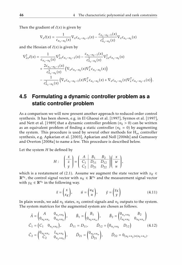
46 4 The characteristic polynomial and rank constraints
Then the gradient of c(x) is given by
∇x c(x) =1
cnx−nk (x)∇xcnx−nk−1(x) −
cnx−nk−1(x)
c2nx−nk (x)
∇xcnx−nk (x)
and the Hessian of c(x) is given by
∇2xx c(x) =
1cnx−nk (x)
∇2xxcnx−nk−1(x) −
cnx−nk−1(x)
c2nx−nk (x)
∇2xxcnx−nk (x)
+2cnx−nk−1(x)
c3nx−nk (x)
(∇xcnx−nk (x)∇Tx cnx−nk (x)
)− 1
c2nx−nk (x)
(∇xcnx−nk−1(x)∇Tx cnx−nk (x) + ∇xcnx−nk (x)∇Tx cnx−nk−1(x)
).
4.5 Formulating a dynamic controller problem as astatic controller problem
As a comparison we will now present another approach to reduced order controlsynthesis. It has been shown, e.g. in El Ghaoui et al. [1997], Syrmos et al. [1997],and Nett et al. [1989] that a dynamic controller problem (nk > 0) can be writtenas an equivalent problem of finding a static controller (nk = 0) by augmentingthe system. This procedure is used by several other methods for H∞ controllersynthesis, e.g. Apkarian et al. [2003], Apkarian and Noll [2006b] and Gumussoyand Overton [2008a] to name a few. This procedure is described below.
Let the system H be defined by
H :
xzy
=
A B1 B2C1 D11 D12C2 D21 D22
xwu
,which is a restatement of (2.1). Assume we augment the state vector with xK ∈Rnk , the control signal vector with uK ∈ Rnk and the measurement signal vector
with yK ∈ Rnk in the following way.
x =(xxK
), u =
(uKu
), y =
(yKy
)(4.11)
In plain words, we add nk states, nk control signals and nk outputs to the system.The system matrices for the augmented system are chosen as follows.
A =(
A 0nx×nk0nk×nx 0nk×nk
), B1 =
(B1
0nk×nw
), B2 =
(0nx×nk B2Ink×nk 0nk×nu
)C1 =
(C1 0nz×nk
), D11 = D11, D12 =
(0nz×nk D12
)(4.12)
C2 =(0nk×nx Ink×nkC2 0ny×nk
), D21 =
(0nk×nwD21
), D22 = 0(nk+ny )×(nk+nu ).

4.5 Formulating a dynamic controller problem as a static controller problem 47
Then assume that we have synthesized a static output feedback controller K forthe system in (4.12). The control signal u is then computed as
u = K y =(KA KBKC KD
)y, (4.13)
where the way the submatrices in K are labeled will be apparent later. This re-sults in the closed loop system equations
˙x = Ax + B1w + B2u
=(A + B2KDC2 B2KC
KBC2 KA
)x +
(B1 + B2KDD21
KBD21
)w,
z = C1x + D11w + D12u
=(C1 + D12KDC2 D12KC
)x +
(D11 + D12KDD21
)w.
The above expressions are equal to the expressions in (2.3). This means that byaugmenting the system and synthesizing a static controller u = K y, we can obtaina dynamic controller for the nonaugmented system using the exact same matricesin the controller, but arranged as suggested by the partitioning in (4.13).
The augmented system contains more states than the nonaugmented system. Thisis not a desired property if we use Theorem 4.1 to synthesize a controller since thedimensions of the variables X and Y increase, which in turn increases the compu-tational burden. However, the dimensions of the matrix K do not increase, whichmakes this procedure suitable for methods that do not involve matrix variablesof the kind that are used in Theorem 4.1. Some references on such methods aree.g. Gumussoy and Overton [2008a] and Apkarian and Noll [2006a], Apkarianand Noll [2006b] and Mammadov and Orsi [2005].
This concludes the background part of this thesis. In the next part we will presentthe suggested methods for low order H∞ controller synthesis.


Part II
Methods
49


5A primal logarithmic barrier method
In this chapter we will describe a primal barrier method that is adapted to theproblem of finding a feasible x for the problem in (4.7). For convex problems,better convergence is obtained from methods using the primal-dual frameworkaccording to Potra and Wright [2000]. However, we consider a primal log-barriermethod mostly because of its straight-forward implementation, see e.g. Boyd andVandenberghe [2004]. The method presented in this chapter consists of bothsolving linear and nonlinear SDPs in order to find a solution. The approach issomewhat ad hoc and some parts are based on empirical results more than asolid theoretical foundation. However, the algorithm has shown to perform quitewell.
This chapter is structured as follows. We begin in Section 5.1 by presenting pub-lished work related to logarithmic barrier methods. Then we present the prob-lem formulation in Section 5.2. We continue by adapting a barrier method tothe problem in Section 5.3–Section 5.5. We summarize all parts of the method inAlgorithm 8 in Section 5.6 and conclude the chapter by a summary in Section 5.7.
5.1 Introduction
The barrier method emerged as a popular interior point algorithm for convexoptimization as early as in the 1960s, and its early history is described in detailin [Fiacco and McCormick, 1968, Chapter 1.2]. Other related techniques are themethod of centers, see Liêu and Huard [1966], and penalty (or exterior point)methods, see [Fiacco and McCormick, 1968, Chapter 4]. The interest for barriermethods decreased in the 1970s due to concerns about ill-conditioning for highvalues of the barrier parameter.
51

52 5 A primal logarithmic barrier method
When the paper on a polynomial-time projective algorithm in Karmarkar [1984]was published, researchers really began to focus on interior point methods. Thebarrier method regained interest when it was pointed out in Gill et al. [1986] thatit had close connection with Karmarkar’s algorithm. Nesterov and Nemirovski[1994] developed the theory of self-concordance, which was shown to be thekey property of a barrier function for the method to achieve polynomial-timecomplexity. They extended the framework for primal logarithmic barrier algo-rithms to also include semidefinite programming (SDP) problems and second-order cone programming (SOCP) problems. A survey paper on interior-pointmethods for convex, conic and general nonlinear optimization can be found inNemirovski and Todd [2008] and a survey paper on numerical methods for large-scale nonlinear optimization in Gould et al. [2005].
As mentioned in the introduction for the thesis, barrier methods have been usedin several algorithms for design of low order H∞ controllers, e.g. Kocvara et al.[2005], Leibfritz and Mostafa [2002], Hol et al. [2003], Thevenet et al. [2005]and Stingl [2006]. However they considered the BMI formulation of the problemin (2.13) as a starting point for their method instead of the LMI formulation in(2.21). The algorithm in Kocvara et al. [2005] was implemented in the softwarePENBMI which is a special version of PENNON. PENNON can be used for gen-eral nonlinear and semidefinite problems, see Kocvara and Stingl [2003].
5.2 Problem formulation
As described in Chapter 4, the problem of finding an H∞ controller of ordernk such that the closed loop system satisfy ‖Hc(s)‖∞ ≤ γ can be formulated assolving the following nonconvex semidefinite program, which is a restatement of(4.7).
minimizex
cnx−nk−1(x)
cnx−nk (x)(5.1a)
subject to Fj (x) = C(j) −m∑i=1
A(j)i xi � 0, j = 1, 2, 3 (5.1b)
If the solution x∗ to (5.1) is such that cnx−nk−1(x)/cnx−nk (x) = 0 and cnx−nk (x) , 0,then x∗ satisfies (4.4) and we can obtain the controller by continuing from step 2in Algorithm 2 from Chapter 2.
5.3 Using the logarithmic barrier formulation
Using Definition 3.8, we can state that the central path for the problem in (5.1) isthe solutions x∗(t), t ≥ 0 to the following minimization problems,
minimizex
tcnx−nk−1(x)
cnx−nk (x)−
∑j=1,2,3
log det Fj (x), (5.2)

5.4 An extra barrier function 53
where we have made the variable substitution t = 1/µ in (3.8) and multiplied by t.The idea for obtaining an approximate solution to (5.1) is to solve (5.2) iterativelyfor a sequence of increasing values of tk . The point x∗(tk−1) can be used in thenext iteration as a starting point for the problem of finding x∗(tk).
It is important to note that since the objective function in (5.1) is a nonconvexfunction, a solution to (5.2) might not be a global solution and thus as t →∞, thesequence x∗(t) might not approach a global solution of the problem (5.1).
5.4 An extra barrier function
In some cases, the problem in (5.2) is unbounded from below, even if the optimalpoint is attainable for the problem in (5.1). This can happen if the set defined bythe inequalities in (5.1b) is not bounded. We can introduce an extra constraintsuch that the set becomes bounded and such that the optimum of the originalproblem in (5.1) is not affected. Consider the following lemma.
Lemma 5.1. For X, Y ∈ Snx , the following constraints define a bounded set.(X II Y
)� 0, (5.3)
trace(X + Y ) < M. (5.4)
where 0 < M < ∞ is an arbitrary constant.
Proof: From the inequality in (5.3) and the nonstrict Schur complement formulain Boyd et al. [1994] follows that X � 0. This and the inequality in (5.4) implythat
0 < Xii < M, i = 1, . . . , nx,
which means that each diagonal element is bounded. Since X � 0, we have foreach submatrix X ∈ S2 of X defined by
X =(Xii XjiXji Xjj
), 1 ≤ i < j ≤ nx,
that X � 0. By using Lemma 2.2, this implies that
Xii − X2ij /Xjj > 0,
which is equivalent to the requirement that
−√XiiXjj < Xij <
√XiiXjj ,
and we have that
−M < Xij < M.
This shows that each element in X is bounded. A similar argument proves thateach element in Y is bounded.

54 5 A primal logarithmic barrier method
To make sure that the set defined by the inequalities in (4.4a)–(4.4c) is bounded,we can use Lemma 5.1 and add the inequality in (5.4) with M chosen as a largenumber. This corresponds to a fourth LMI for the problem in (5.1). The constantM should be chosen large enough such that the solution to the modified problemis the same as the solution to the original problem.
To derive the fourth LMI for the problem in (5.1), write the inequality in (5.4) as
M − trace(X + Y ) > 0. (5.5)
Then by using the half-vectorization operator vech, see Definition 4.1, we makethe variable substitution
x =(vech(X)vech(Y )
).
By defining
IXY =(vech(Inx )vech(Inx )
), (5.6)
we can write the inequality in (5.5) as
F4(x) = M − ITXY x > 0.
Now we can construct an extra logarithmic barrier function as
ψ4(x) = − log F4(x), (5.7)
which is added to (5.2) and results in the following modified problem.
minimizex
B(x, t) = tcnx−nk−1(x)
cnx−nk (x)−
∑j=1,2,3
log det Fj (x) − log F4(x). (5.8)
One must make sure that the extra barrier function does not create any falseoptimum. This may happen if the true optimum lies outside the extra barrier. Incase that happens, we can enlarge the extra barrier, i.e., increase M, and solveagain. However, M = 104 seems to work well in numerical evaluations.
5.5 Outlining a barrier based method
We will now focus on the problem in (5.8) and outline a barrier based methodfor solving it iteratively as t → ∞. In the limit, the solution x∗ to the problem in(5.8) will approach a local optimum of the problem in (5.1). The method inter-changeably uses Algorithm 4 in Section 3.5.4 and a standard linear SDP solverfor finding the initial point. The decision of when to switch between the methodsis motivated by a mix of theory, intuition and experimental results. The impactof balancing the system, as described in Section 2.4, has appeared to be of greatimportance for the algorithm to work efficiently, and therefore has a central rolein the algorithm.

5.5 Outlining a barrier based method 55
5.5.1 Initial point calculation
Since Newton’s method (Algorithm 4) is applied to the problem in (5.8), it needsto be initialized with a feasible starting point. An initial point x0 can be calcu-lated by solving the following problem, which is also a heuristic method for ob-taining low rank solutions, as mentioned in e.g. Iwasaki [1999], Orsi et al. [2006],and Fazel et al. [2001].
x0 = argminx
ITXY x(
= trace(X + Y ))
(5.9a)
subject to Fj (x) = C(j) −m∑i=1
A(j)i xi � 0, j = 1, 2, 3. (5.9b)
This is the same optimization problem as in (5.1) but with another objective func-tion. The problem in (5.9) is a standard linear SDP, and it can be solved using thesoftware packages SDPT3, Toh et al. [2006], and YALMIP, Löfberg [2004].
After solving the problem in (5.9), the system is balanced around X0, Y0, as de-scribed in Section 2.4, in order to make the problem better conditioned. Then,the problem is reformulated using the new system matrices and the initial pointcalculation is done again.
5.5.2 Solving the main, nonconvex problem
Now we have a feasible starting point, and we can apply Newton’s method (Algo-rithm 4), to the, now numerically balanced, problem in (5.8). However, we stillneed to discuss the choice of t, and especially how to initialize t.
In order to simplify notation in later sections, we introduce the following defini-tions. Let
f (x) =cnx−nk−1(x)
cnx−nk (x)and φ(x) = −
∑j=1,2,3
log det Fj (x) − log F4(x). (5.10)
Choosing the barrier parameter
When starting the algorithm, we need to choose an initial value of the barrierparameter, t0. In [Boyd and Vandenberghe, 2004, page 570], a method is sug-gested which is based on a minimization of a measure of fulfilling the optimalityconditions for being on the central path with respect to t. The result is
t0 = argmint
(t∇xf (x0) + ∇xφ(x0)
)TH−1
(t∇xf (x0) + ∇xφ(x0)
)(5.11)
where x0 is the initial point and H � 0 is some matrix that defines a norm, forinstance the Hessian
∇2xxB(x, t) = t∇2
xxf (x0) + ∇2xxφ(x0)
could be used, where B(x, t) is defined in (5.8). The problem is, ∇2xxf (x0) need
not be positive definite, which may cause problems. One may assume that in the

56 5 A primal logarithmic barrier method
beginning, t is usually small, and could be approximated as zero. This will alsoguarantee that the minimization problem is convex, since we then have that
∇2xxB(x, 0) = ∇2
xxφ(x0) � 0.
Here, the extra barrier in (5.7) need not be included, because its contributioncan be approximated as zero, if M is chosen appropriately big. If we simplifynotation by writing ∇f0 = ∇xf (x0) and ∇φ0 = ∇xφ(x0), the problem in (5.11) canthen be written as
t0 = argmint
t2(∇f0)TH−1∇f0 + 2t∇f T0 H−1∇φ0 + (∇φ0)TH−1∇φ0, (5.12)
which is a scalar quadratic problem. The solution can be written explicitly as
t0 = −∇f0H−1∇φ0
∇f T0 H−1∇f0. (5.13)
For k ≥ 1, the barrier parameter is updated in a standard way as
tk = µtk−1, (5.14)
where µ = 10 has shown to work quite well.
Interference of bad scaling
We must make sure that the extra barrier, which was described in Section 5.4,will not interfere with the convergence of the algorithm to an optimal point ofthe original problem in (5.1) that we want to solve. Consequently, we test if
ITXY x > kMM,
where 0 < kM < 1. When this condition is satisfied, it is assumed that this is dueto bad scaling, since M is chosen to be big enough. Then we balance the problemaround Xk , Yk and restart the algorithm once again by choosing an initial pointas described in Section 5.5.1, and proceed from there.
Dealing with the nonconvexity
When using a Newton method, to get a descent direction, the Hessian must bepositive definite, as described in Section 3.5.1. If that is not the case, one may useany of the methods presented in Section 3.5.3 to create an approximate Hessianthat is positive definite. An alternative to these methods is to use some specialproperties of the problem. Since the constraints define a convex set, the barrierfunction is convex, and hence the Hessian of the barrier function will be positivedefinite. The total Hessian will be
∇2xxB(x, t) = t∇2
xxf (x) + ∇2xxφ(x), (5.15)
where the first term on the right hand side might be indefinite but the second oneis always positive definite. Therefore, we can modify the Hessian as
H(x, t, a) = taH t∇2xxf (x) + ∇2
xxφ(x), (5.16)

5.6 The logarithmic barrier based algorithm 57
where 0 < tH < 1 and a is a non-negative integer chosen such that H(x, t, a) � 0.We know that at least in the limit, a→∞, this will be true.
5.5.3 Stopping criteria
The presented algorithm consists of inner and outer iterations. The inner itera-tions are described by Algorithm 4, where the stopping criterion is some functionof the Newton decrement, Λ(x). For each outer iteration, the solution of (5.8)gives a point on the central path. The stopping criteria are as follows.
1. The algorithm is exceeding the maximum number of inner or outer itera-tions. This is the case if the algorithm has slow or no progress, thus thealgorithm terminates. A solution to this problem could be to reformulatethe problem, e.g. increase the performance measure γ , and restart the algo-rithm. However, this needs to be done manually.
2. The extra barrier is interfering as discussed in the previous section, i.e.,
ITXY x > kMM, 0 < kM < 1.
Re-balance the problem around the current iterate (Xk , Yk) and restart thealgorithm by following the procedure described in Section 5.5.1, and pro-ceed from there.
3. The objective function value is close to zero,
cnx−nk−1(x)
cnx−nk (x)< ε,
i.e., we have found an optimum to the problem (5.1) with accuracy ε.
5.6 The logarithmic barrier based algorithm
Now all parts of the algorithm have been described, and we can put them togetherinto a complete algorithm, which is presented as Algorithm 8.
5.6.1 Optimality of the solution
Note that the optimality conditions are not necessarily satisfied when this algo-rithm finishes. This is due to the inner loop stopping criterion, which is a direc-tional derivative. The only KKT condition for the unconstrained problem is thatthe gradient should be zero, which need not be true just because a directionalderivative is.
However, the point x∗ need not be optimal, just sufficiently good. When the algo-rithm finishes with success, the achieved solution is always feasible for (5.1) andthe objective function is sufficiently small, i.e., near zero, which means that wehave found a solution (with accuracy ε), to the original feasibility problem (4.4).

58 5 A primal logarithmic barrier method
5.6.2 Finding the controller
When we have found a local optimal point x∗ or equivalently, (X∗, Y ∗), we nowneed to find a controller, which is a convex problem. To do so we proceed fromStep 2 in Algorithm 2, i.e., recover the variable P as described in Section 2.5.
5.6.3 Algorithm performance
The performance of the algorithm will be investigated in Chapter 8, where wewill apply Algorithm 8 to a set of test problems. Comparisons will be made witha primal-dual method, which will be described in Chapter 6, as well as with amethod from literature, Hifoo, which is briefly presented in Section 8.1.2.
5.7 Chapter summary
In this chapter a primal logarithmic barrier method for design of low order H∞controllers is suggested. The algorithm is initialized by solving a semidefinite pro-gramming problem corresponding to a heuristic for finding low rank solutions.In each outer iteration the main algorithm attempts so find a local minimum to anunconstrained problem using Newton’s method with a line search. As the barrierparameter tends to infinity, the aim is to find a feasible solution that correspondsto a low order controller with performance measure γ . A numerical evaluationof the algorithm is presented in Chapter 8.

5.7 Chapter summary 59
Algorithm 8 The barrier algorithm
Given performance criteria γ and system matrices A, B, C, D, formulate theproblem.Choose parameter M.Calculate an initial point x0, as in Section 5.5.1.Calculate an initial value t0, of the barrier parameter as in Section 5.5.2.kinner := 0, kouter := 0while cnx−nk−1(xk)/cnx−nk (xk) < ε dokouter := kouter + 1while 1 do
Calculate gradient, gk = ∇xB(xk , tk) and Hessian Hk = H(xk , tk , ak).Find integer ak ≥ 0 such that Hk � 0, according to (5.16).Solve for the Newton step: Hkpk = −gk .Perform backtracking line search to find α.xk+1 := xk + αpkCalculate Newton decrement: Λ =
√−gkpkkinner := kinner + 1if Λ < Λtol then
Satisfying tolerance for the Newton decrement, exit inner loop.end ifif kinner ≥ kinner, max then
Abort, too many inner iterations.end if
end while (Inner loop)if kouter ≥ kouter, max then
Abort, too many outer iterations.end ifCheck for bad scaling, see Section 5.5.2. Re-balance and restart if necessary.t := µt
end while (Outer loop)Success!


6A primal-dual method
In this chapter we will describe a primal-dual interior point method for low orderH∞ controller synthesis. The method appears in two versions that are named theprimal-dual method and the quasi-Newton method. The second method is basedon the first one and the main difference is that the Hessian calculations are carriedout using damped BFGS updating.
The presentation in this chapter is based on relevant chapters in Nocedal andWright [2006] and Todd et al. [1998].
This chapter is structured as follows. We begin in Section 6.1 by presentingpublished work for solving semidefinite programming problems with focus onprimal-dual methods. Then we present the problem formulation in Section 6.2and the optimality conditions in Section 6.3. In Section 6.4 and Section 6.5 we de-scribe the different parts of a Mehrotra primal-dual method. We summarize ourmethod in Algorithm 9 in Section 6.6 and conclude the chapter by a summary inSection 6.7.
6.1 Introduction
Since primal-dual methods are also interior point methods, they share their earlyhistory with primal logarithmic barrier methods, which is briefly presented inSection 5.1. In Meggido [1988] a framework for primal-dual algorithms wasdescribed, which was originally published in 1987. Mehrotra [1992] presenteda practical algorithm for linear programming that remains the basis for mostcurrent software. This work was extended to semidefinite programming (SDP)and second-order cone programming (SOCP) in the work by Nesterov and Todd[1997, 1998].
61
62 6 A primal-dual method
Forsgren and Gill [1998] and Vanderbei and Shanno [1999] present methods thatextend primal-dual interior theory for linear and quadratic programming to non-convex nonlinear programming. For a survey on interior point methods for non-linear optimization, see Forsgren et al. [2002].
A method for solving nonconvex semidefinite programming was proposed inJarre [2000]. It combines features of trust-region methods, sequential quadraticprogramming (SQP) methods and predictor-corrector interior point methods. InFreund et al. [2007] a sequential semidefinite programming (SSP) method waspresented, which generalizes the SQP method for standard nonlinear programs.This method have some parts in common with primal-dual methods for semidef-inite programming.
One approach for solving nonconvex semidefinite programming problems is Kan-zow et al. [2005], which is a successive linearization method for nonlinear semi-definite programs with a trust-region framework. Another approach is presentedin Correa and Hector Ramirez [2005], which is a method inspired by the SQPmethod. It solves a quadratic SDP in each iteration to get the search directionand then uses a nondifferentiable merit function combined with a line searchstrategy.
Algorithms for solving optimization problems defined on a subset of the coneof symmetric positive matrices are presented in Burer and Monteiro [2003] andJournée et al. [2010]. Those algorithms rely on the factorization X = Y Y T , whereY ∈ Rn×r and r < n, hence resulting in low rank solutions of the problem.
In Yamashita et al. [2011], a primal-dual interior point method is presented thatminimizes a nonconvex function subject to linear semidefinite constraints. Theysuggest two versions of their method, where one uses an exact Hessian while theother uses a BFGS update of the Hessian. The approach in this chapter is similar,however we were unaware of this work until very recently.
For a reference on primal-dual interior point methods for linear programming,see e.g. the book by Wright [1997]. For a survey of sequential quadratic program-ming, see Boggs and Tolle [1995], for a survey on semidefinite optimization, seeTodd [2001] and for a more general survey on interior point methods for opti-mization, see Nemirovski and Todd [2008].
6.2 Problem formulation
As described in Chapter 4, the problem of finding an H∞ controller of ordernk such that the closed loop system satisfy ‖Hc(s)‖∞ ≤ γ can be formulated assolving the following nonconvex semidefinite program, which is a restatement of

6.3 Optimality conditions 63
(4.7) or (5.1).
minimizex
cnx−nk−1(x)
cnx−nk (x)(6.1a)
subject to C(j) −m∑i=1
A(j)i xi � 0, j = 1, 2, 3. (6.1b)
If the solution x∗ to (6.1) is such that cnx−nk−1(x)/cnx−nk (x) = 0 and cnx−nk (x) , 0,this means that x∗ satisfies (4.4) and we can obtain the controller by continuingfrom step 2 in Algorithm 2 from Chapter 2. To keep the notation simple, define
f (x) =cnx−nk−1(x)
cnx−nk (x),
and merge the three semidefinite constraints in (6.1b) into one constraint by plac-
ing the matrices C(j) and A(j)i in block diagonal matrices consisting of three blocks,
one for each value of j. This results in
minimizex
f (x)
subject to C −m∑i=1
Aixi � 0.(6.2)
Note that the constraints are merged to simplify notation. It is advisable to utilizethe block structure in order not to increase the number of variables at a later stagewhen dual and slack variables are introduced.
6.3 Optimality conditions
The first-order necessary conditions for optimality, see Theorem 3.1, have a verycentral role in primal-dual methods. The Karush-Kuhn-Tucker conditions for(6.2) are given by
df (x)dxi
+ 〈Ai , Z〉 = 0, i = 1, . . . , m (6.3a)
C −m∑i=1
Aixi − S = 0, (6.3b)
ZS = 0, (6.3c)
Z � 0, S � 0, (6.3d)
where Z ∈ Sp is a dual variable and S ∈ Sp is a slack variable of appropriatedimension p. Note that (6.3a) consists of m scalar equations, while (6.3b)–(6.3c)are matrix equations. Since f (x) is a nonconvex function, these are only necessaryand not sufficient conditions for an optimal solution of (6.2).

64 6 A primal-dual method
6.4 Solving the KKT conditions
As mentioned previously, the main idea of primal-dual methods is to find a solu-tion to the KKT conditions. The way it is usually done is to search for solutionsalong the central path.
6.4.1 Central path
The central path (as defined in Definition 3.12) for the problem in (6.2) is thesolution points for
df (x)dxi
+ 〈Ai , Z〉 = 0, i = 1, . . . , m (6.4a)
C −m∑i=1
Aixi − S = 0, (6.4b)
ZS = νI, (6.4c)
Z � 0, S � 0, (6.4d)
where ν ≥ 0. The difference from (6.3) is the third equation. When solving theequations for the KKT conditions in (6.3), we generate a sequence of iterates
x(k) = (x(k), Z(k), S(k)),
that solve (6.4a)–(6.4c) for values of ν that tend to zero. The iterates need notnecessarily be feasible, except for (6.4d), which always must hold.
6.4.2 Symmetry transformation
Since the domain and range of the function defined by the left hand side ofthe equation in (6.4c) is not the same space, we cannot directly apply Newton’smethod, as described in Section 3.6.1, to the system of equations defined by(6.4a)–(6.4c). A solution for this is to use the symmetry transformation in Zhang[1998] which is defined as
HP (M) =12
(PMP −1 + (PMP −1)T ) (6.5)
for a given invertible matrix P . It is shown that if M is similar to a symmetricpositive definite matrix, then
HP (M) = νI ⇔ M = νI.
This means that (6.4c) can be replaced by
HP (ZS) = νI (6.6)
without affecting the definition of the central path, since ZS is similar to thepositive definite matrix S1/2ZS1/2. The equations in (6.4a), (6.4b) and (6.6) canbe written as F(x) = 0 for some F and x. Now we can apply Newton’s method fornonlinear equations to F(x). We denote the step that minimizes the linear model

6.4 Solving the KKT conditions 65
as (∆x,∆Z,∆S) and obtain the follow equations that define the step.
df (x)dxi
+ 〈Ai , Z〉 +ddxi∇Tx f (x)∆x + 〈Ai ,∆Z〉 = 0, i = 1, . . . , m (6.7a)
C −m∑i=1
Aixi − S −m∑i=1
Ai∆xi − ∆S = 0, (6.7b)
HP (ZS) +HP (∆ZS + Z∆S) − νI = 0. (6.7c)
The scaling matrix P which is used in the symmetrization operator, can be chosenin several ways which has given rise to different methods, e.g. the Nesterov-Todd(NT) method, given in Nesterov and Todd [1997, 1998], the AHO method in Al-izadeh et al. [1998] and the H..K..M method, see Helmberg et al. [1996], Kojimaet al. [1997], Monteiro [1997]. For a presentation of how to calculate these scalingmatrices and some numerical experiments using them, see Todd et al. [1998].
In this work, we chose the Nesterov-Todd (NT) scaling matrix since it has shownto perform well in applications, see e.g. Todd et al. [1998]. To compute the NTscaling matrix, begin by Cholesky factorizing Z and S as
Z = LLT , S = RRT , (6.8)
and let UDV T = RT L be the SVD of RT L. Then the NT scaling matrix is given by
P = LVD−1/2. (6.9)
As can be seen here, the scaling matrix depends on Z and S and must thereforebe recalculated in each iteration.
6.4.3 Definitions
Before we move on, we define the symmetric vectorization operator svec and thesymmetric Kronecker product.
Definition 6.1 (svec). The operator svec : Sn → Rn(n+1)/2 is defined by
svec(U ) = (u11,√
2u21, . . . ,√
2un1, u22,√
2u32, . . . ,√
2un2, . . . , unn)T , (6.10)
i.e., svec is an operator that maps symmetric matrices into vectors. The factor√
2is introduced so that svec is an isometry between S
n×n and Rn(n+1)/2 with their
respective standard inner products. Let the inverse of svec be denoted smat.
Note that the operator svec is different from the operator vech in Definition 4.1,since svec scales the nondiagonal entries by
√2.
Example 6.1Let us illustrate the operator svec by a simple example. If we let
U =
1 2 32 4 53 5 6
,

66 6 A primal-dual method
then
svec(U ) =(1, 2√
2, 3√
2, 4, 5√
2, 6)T,
and the inner products
〈U,U〉 = trace(U TU ) = 129,
〈svec(U ), svec(U )〉 = svec(U )T svec(U ) = 129,
are the same.
Definition 6.2 (Symmetric Kronecker product). Let A and B be two real ma-trices of dimension n × n. The symmetric Kronecker product of A and B is thendefined as
A ⊗S B =12U (A ⊗ B + B ⊗ A)U T , (6.11)
where U ∈ Rn(n+1)×n2is a matrix created in the following way. If we label the
rows of U in the order (1, 1), (2, 1), . . . , (n, 1), (2, 2), (3, 2), . . . , (n, 2), (3, 3) . . . , (n, n)and its columns in the order (1, 1), (2, 1), . . . , (n, 1), (1, 2), . . . , (n, 2), (1, 3), . . . , (n, n),then
U(i,j),(k,l) =
1 if i = j = k = l,
1/√
2 if i = k , j = l, or i = l , j = k,
0 otherwise.
See e.g. the appendix of Todd et al. [1998] for properties and details regardingthe symmetric Kronecker product.
Example 6.2When n = 3, the matrix U in (6.11) is given by
U =
1 0 0 0 0 0 0 0 00 1/
√2 0 1/
√2 0 0 0 0 0
0 0 1/√
2 0 0 0 1/√
2 0 00 0 0 0 1 0 0 0 00 0 0 0 0 1/
√2 0 1/
√2 0
0 0 0 0 0 0 0 0 1
.
6.4.4 Computing the search direction
To compute the Newton step (∆x,∆Z,∆S), it is convenient to express the linearsystems of equations in the standard matrix vector form. Using the previouslydefined symmetric vectorization operator and symmetric Kronecker product, we
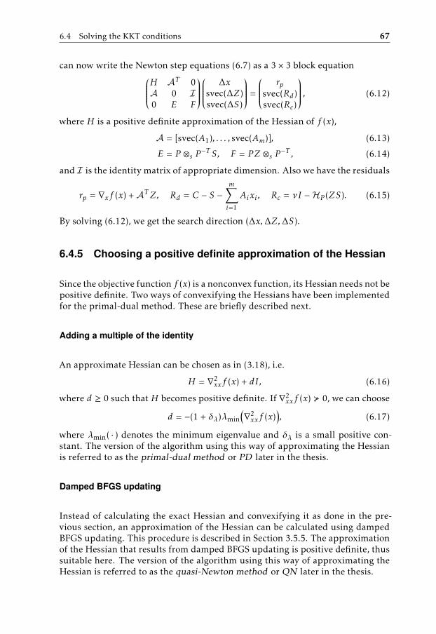
6.4 Solving the KKT conditions 67
can now write the Newton step equations (6.7) as a 3 × 3 block equationH AT 0A 0 I0 E F
∆xsvec(∆Z)svec(∆S)
=
rpsvec(Rd)svec(Rc)
, (6.12)
where H is a positive definite approximation of the Hessian of f (x),
A = [svec(A1), . . . , svec(Am)], (6.13)
E = P ⊗s P −T S, F = P Z ⊗s P −T , (6.14)
and I is the identity matrix of appropriate dimension. Also we have the residuals
rp = ∇xf (x) + AT Z, Rd = C − S −m∑i=1
Aixi , Rc = νI − HP (ZS). (6.15)
By solving (6.12), we get the search direction (∆x,∆Z,∆S).
6.4.5 Choosing a positive definite approximation of the Hessian
Since the objective function f (x) is a nonconvex function, its Hessian needs not bepositive definite. Two ways of convexifying the Hessians have been implementedfor the primal-dual method. These are briefly described next.
Adding a multiple of the identity
An approximate Hessian can be chosen as in (3.18), i.e.
H = ∇2xxf (x) + dI, (6.16)
where d ≥ 0 such that H becomes positive definite. If ∇2xxf (x) � 0, we can choose
d = −(1 + δλ)λmin
(∇2xxf (x)
), (6.17)
where λmin( · ) denotes the minimum eigenvalue and δλ is a small positive con-stant. The version of the algorithm using this way of approximating the Hessianis referred to as the primal-dual method or PD later in the thesis.
Damped BFGS updating
Instead of calculating the exact Hessian and convexifying it as done in the pre-vious section, an approximation of the Hessian can be calculated using dampedBFGS updating. This procedure is described in Section 3.5.5. The approximationof the Hessian that results from damped BFGS updating is positive definite, thussuitable here. The version of the algorithm using this way of approximating theHessian is referred to as the quasi-Newton method or QN later in the thesis.

68 6 A primal-dual method
6.4.6 Uniqueness of symmetric search directions
To prove that the symmetric search directions that we obtain from solving (6.12)are unique, we show that the only solution to the 3 × 3 block equationH AT 0
A 0 I0 E F
∆xsvec(∆Z)svec(∆S)
= 0 (6.18)
is the trivial zero solution. Since P is an invertible matrix and Z, S � 0, by Theo-rem 3.2 in Todd et al. [1998], we have that E−1F � 0. Further, we can assume thatE and F are invertible, by using properties of the symmetric Kronecker product(see Appendix of Todd et al. [1998] for details). Using block Gaussian eliminationwe can reduce (6.18) to a Schur complement equation
(H +AT E−1FA)∆x = 0. (6.19)
Since H � 0 and AT E−1FA � 0 regardless of the rank of A, (H + AT E−1FA) � 0is invertible and the only solution to (6.19) is the trivial solution. Now the secondblock equation of (6.18) gives that ∆S = − smat(A∆x) = 0, and the third onegives that ∆Z = −E−1F∆S = 0. This shows that the solution to (6.12) exists andis unique.
6.4.7 Computing step lengths
Once a search direction (∆x,∆Z,∆S) is found, the next step is to determine howfar to go in that direction. Step lengths 0 < α ≤ 1 and 0 < β ≤ 1 are chosen suchthat
Z(k+1) = Z(k) + α∆Z � 0, S(k+1) = S(k) + β∆S � 0, (6.20)
i.e., such that the positive definiteness is maintained for the symmetric variablesZ and S. The variable x is updated as
x(k+1) = x(k) + β∆x.
We use the fraction to boundary rule, see e.g. Nocedal and Wright [2006], whichmeans that we do not let the next iterate end up at the boundary of semidefinite-ness, but instead only near it. One way to do this is to choose the step lengthsas
α(k) = min(1,
−τ (k)
λ−min(L−1∆ZL−T )
), β(k) = min
(1,
−τ (k)
λ−min(R−1∆SR−T )
), (6.21)
with L and R chosen as in (6.8) and where λ−min(A) denotes the minimum eigen-value of A. If all eigenvalues are positive the term is ignored, i.e., the step lengthis chosen to be 1, regardless of the value of the min( · , · ) expressions. The param-eter τ is chosen based on the step lengths taken in the previous iteration, i.e., bysetting
τ (k+1) = 0.9 + 0.09 min(α(k), β(k)), (6.22)

6.5 A Mehrotra predictor-corrector method 69
Z1
Z2
Z
Z + ∆Z
(a)
Z1
Z2
Z
Z + ∆Z
Z + α∆Z
Z + α∆Z
(b)
Figure 6.1: The two figures above illustrate the case where the cone is R2+.
To the left, the full step does not take us outside of the cone. In the figureto the right we apply the fraction to boundary rule. If τ = 1, the resultingstep length parameter is α and we end up at the boundary. The number α iscalculated using τ < 1 and we end up at some distance from the boundaryinstead.
where α(k) and β(k) are the step lengths in the kth iteration. An initial valueτ (0) = 0.98 has shown to work well. The fraction to boundary rule is illustratedin Figure 6.1.
6.5 A Mehrotra predictor-corrector method
In this section we will describe the steps of an algorithm based on Mehrotra’salgorithm, see Mehrotra [1992], however we follow the presentation in the papersby Todd et al. [1998] and Toh et al. [1999] which extend Mehrotra’s algorithm tosemidefinite programming.
6.5.1 Initial point calculation
Always when solving optimization problems, a good initial point is important.For convex problems it will have an impact on the number of iterations needed,and for nonconvex problems it also determines which KKT-point the algorithmwill converge to.
The initial point calculation used for the primal-dual method is based on what issuggested in Toh et al. [1999] and will be described below.
Assume the matrices Ai and C are block-diagonal of the same structure, each
consisting of L blocks of square matrices of dimensions n1, n2, . . . , nL. Let A(j)i

70 6 A primal-dual method
and C(j) denote the jth block of Ai and C, respectively. Then the initial point canbe chosen as
x(0) = 1,
Z(0) = blkdiag(ξ1In1, ξ2In2
, . . . , ξLInL ),
S(0) = blkdiag(η1In1, η2In2
, . . . , ηLInL ),
(6.23)
where 1 is a column vector containing ones, Inj is the identity matrix with dimen-sion nj and
ξj = nj max1≤i≤m
1 + |bi |
1 + ||A(j)i ||F
, ηj =1 + max[maxi{||A
(j)i ||F}, ||C
(j)||F]√nj
,
where b is referring to the linear objective function which in our case is
b =(vech(In)vech(In)
)(6.24)
so that
bT x = trace(X + Y ), (6.25)
i.e., we follow the heuristics for minimizing rank as mentioned in e.g. Iwasaki[1999], Orsi et al. [2006], and Fazel et al. [2001]. The only difference from Tohet al. [1999] is that the authors suggest x(0) = 0, but our choice has shown to workbetter in our applications. By multiplying the identity matrix Inj by the factorsξj and ηj for each j, the initial point has a better chance of having the same orderof magnitude as an optimal solution of the SDP according to Toh et al. [1999].
Note that the assumption that Ai and C are block-diagonal is valid since wemerged three constraints into one, as explained in Section 6.2.
6.5.2 The predictor step
Set ν = 0 in (6.15), solve the system of equations in (6.12) and denote the solution(∆xaff,∆Zaff,∆Saff). This step is sometimes called the predictor step or affinescaling step. Then calculate step lengths αaff, βaff as done in (6.21). Define µ andµaff as
µ = 〈Z, S〉/p, (6.26)
µaff = 〈Z + αaff∆Zaff, S + βaff∆Saff〉/p, (6.27)
and the centering parameter σ as
σ =(µaff
µ
)e, (6.28)
The exponent e is chosen according to
e =
max(1, 3 min(αaff, βaff)2
)if µ > 10−6,
1 if µ ≤ 10−6,(6.29)

6.6 The primal-dual algorithm 71
which is a heuristic suggested in Toh et al. [1999] that does not have a solid ana-lytical justification, but appears to work well in practice.
Note that the algorithm does not update the iterate with the predictor step. It isonly used to calculate the centering parameter, σ , which is needed for the com-putation of the corrector step, which will be described next.
6.5.3 The corrector step
The search direction is now calculated by solving (6.12) again but replacing Rcwith
Rs = σµI − HP (ZS) − HP (∆Zaff∆Saff), (6.30)
where µ and σ are calculated as in (6.26) and (6.28) respectively. The previouslycalculated predictor step (∆Zaff,∆Saff) is used in a second-order correction, seeTodd et al. [1998], where it is assumed that the predictor step is a decent approx-imation of the corrector step. This will result inH AT 0
A 0 I0 E F
∆xsvec(∆Z)svec(∆S)
=
rpsvec(Rd)svec(Rs)
, (6.31)
with the submatrices and vectors defined in (6.13)–(6.15). The coefficient matrixin (6.31) is the same as in the calculation of the predictor step in (6.12), and hencethe cost of solving the second system can be made relatively small since the samematrix factorization can be used in both cases.
6.6 The primal-dual algorithm
By summarizing the last few sections we can now state an algorithm as Algo-rithm 9. Define the residual
r(x, Z, S, ν) =
rp(x, Z)
svec(Rd(S, x)
)svec
(Rc(Z, S, ν)
) (6.32)
with ν = 0, where rp, Rd and Rc are calculated as in (6.15). This expression isused in a stopping criterion in the algorithm.
6.6.1 Finding the controller
If the algorithm finishes with f (x) = 0, we can recover the controller parametersby solving a convex problem. To do so we proceed from Step 2 in Algorithm 2 inChapter 2, i.e., recover the variable P as described in Section 2.5.
6.6.2 Algorithm performance
The performance of the algorithm is evaluated in Chapter 8 where two evalu-ations are made. In the first evaluation, the primal-dual method is comparedwith the primal logarithmic barrier method from Chapter 5 and with a method

72 6 A primal-dual method
Algorithm 9 The primal-dual algorithm
Calculate the initial point (x(0), Z(0), S(0)) as explained in Section 6.5.1.Set τ (0) = 0.98, k := 0.
while ||r(x(k), Z(k), S(k), 0)||2 < rtol doif k > kmax then
Abort, too many iterations.end if
Predictor step:Set (x, Z, S) = (x(k), Z(k), S(k)).Solve (6.12) for (∆xaff,∆Zaff,∆Saff) with ν = 0.Calculate step lengths αaff, βaff using (6.21).Calculate µ and µaff using (6.26) and (6.27).Set centering parameter to σ = (µaff/µ)e where e is calculated as in (6.29).
Corrector step:Solve (6.31) for (∆x,∆Z,∆S).Calculate step lengths α, β using (6.21).Set (x(k+1), Z(k+1), S(k+1)) = (x + β∆x, Z + α∆Z, S + β∆S).Calculate τ (k+1) using (6.22).Set k := k + 1.
end while
from literature, Hifoo, which is briefly presented in Section 8.1.2. In the secondevaluation, the quasi-Newton method is compared with Hifoo.
6.7 Chapter summary
I this chapter a primal-dual method for design of low order H∞ controllers issuggested. The starting point of the algorithm is chosen based on heuristics forfinding low rank solutions. When the starting point has been chosen, a Mehrotrapredictor-corrector is applied to the problem. When the algorithm finishes withsuccess, the KKT conditions are satisfied to a specified accuracy, and a controllerof low order with performance measure γ is found. A numerical evaluation ofthe algorithm is presented in Chapter 8.
7A partially augmented Lagrangian
method
In this chapter we will present a partially augmented Lagrangian method for loworder H∞ synthesis. It is a similar method to the augmented Lagrangian methodthat was presented in Section 3.7.2, but partially refers to the fact that some, andin our case only one of the constraints is relaxed while the others are kept asconstraints. References on the standard augmented Lagrangian method can befound in Section 3.7.2.
One main difference in the approach as compared to the algorithms that werepresented in Chapter 5 and Chapter 6 is that this algorithm explicitly tries tominimize the performance measure γ instead of finding a controller that satisfiesa pre-specified value. Parts of this chapter was also presented in Ankelhed et al.[2011b].
This chapter is structured as follows. In Section 7.1 we present published workrelated to partially augmented Lagrangian methods. Then the problem formu-lation is presented in Section 7.2, and how the partially augmented Lagrangianmethod is applied is described in Section 7.3. In Section 7.4 we present howthe search direction is calculated, and in Section 7.5 the suggested algorithm isoutlined. In Section 7.6 the chapter is summarized.
7.1 Introduction
In Conn et al. [1991] the problem of minimizing an augmented Lagrangian func-tion subject to simple bound constraints was considered. In Conn et al. [1996]the work was extended to include linear inequality constraints, where also localand global convergence of the algorithm were proved.
73
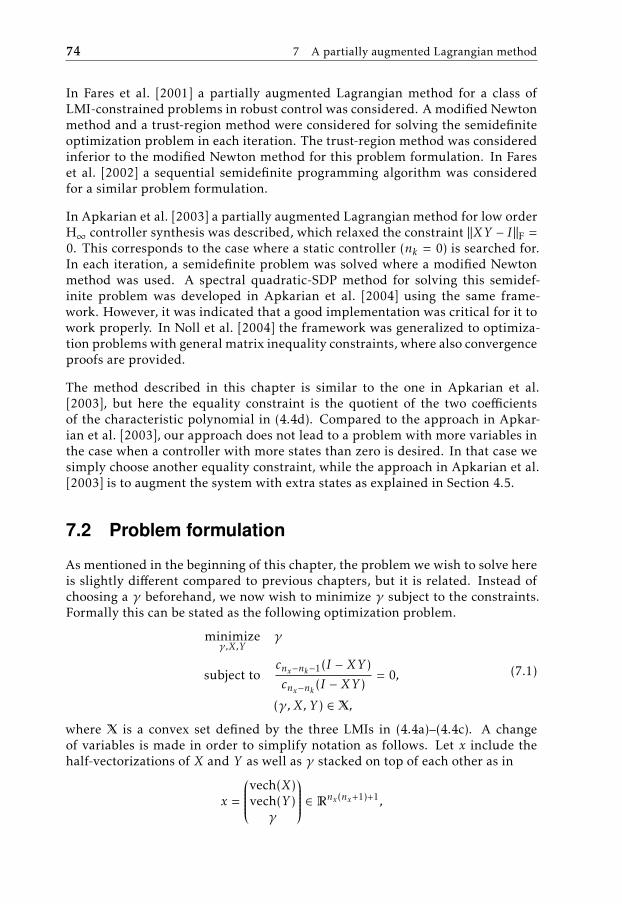
74 7 A partially augmented Lagrangian method
In Fares et al. [2001] a partially augmented Lagrangian method for a class ofLMI-constrained problems in robust control was considered. A modified Newtonmethod and a trust-region method were considered for solving the semidefiniteoptimization problem in each iteration. The trust-region method was consideredinferior to the modified Newton method for this problem formulation. In Fareset al. [2002] a sequential semidefinite programming algorithm was consideredfor a similar problem formulation.
In Apkarian et al. [2003] a partially augmented Lagrangian method for low orderH∞ controller synthesis was described, which relaxed the constraint ‖XY − I‖F =0. This corresponds to the case where a static controller (nk = 0) is searched for.In each iteration, a semidefinite problem was solved where a modified Newtonmethod was used. A spectral quadratic-SDP method for solving this semidef-inite problem was developed in Apkarian et al. [2004] using the same frame-work. However, it was indicated that a good implementation was critical for it towork properly. In Noll et al. [2004] the framework was generalized to optimiza-tion problems with general matrix inequality constraints, where also convergenceproofs are provided.
The method described in this chapter is similar to the one in Apkarian et al.[2003], but here the equality constraint is the quotient of the two coefficientsof the characteristic polynomial in (4.4d). Compared to the approach in Apkar-ian et al. [2003], our approach does not lead to a problem with more variables inthe case when a controller with more states than zero is desired. In that case wesimply choose another equality constraint, while the approach in Apkarian et al.[2003] is to augment the system with extra states as explained in Section 4.5.
7.2 Problem formulation
As mentioned in the beginning of this chapter, the problem we wish to solve hereis slightly different compared to previous chapters, but it is related. Instead ofchoosing a γ beforehand, we now wish to minimize γ subject to the constraints.Formally this can be stated as the following optimization problem.
minimizeγ,X,Y
γ
subject tocnx−nk−1(I − XY )
cnx−nk (I − XY )= 0,
(γ, X, Y ) ∈ X,
(7.1)
where X is a convex set defined by the three LMIs in (4.4a)–(4.4c). A changeof variables is made in order to simplify notation as follows. Let x include thehalf-vectorizations of X and Y as well as γ stacked on top of each other as in
x =
vech(X)vech(Y )
γ
∈ Rnx(nx+1)+1,

7.3 The partially augmented Lagrangian 75
where vech is defined in Definition 4.1. This is similar to what is done in Sec-tion 4.3.2 but the difference is that we include γ in x, since γ is now an optimiza-tion variable. This results in the following equivalent problem formulation.
minimizex
bT x
subject tocnx−nk−1(x)
cnx−nk−1(x)= 0,
x ∈ X,
(7.2)
where b is the last unit vector, i.e.
bT =(0 . . . 0 1
),
such that bT x = γ . We realize that stating the equivalence of (X, Y , γ) ∈ X tox ∈ X is abuse of notation.
7.3 The partially augmented Lagrangian
After defining c(x) as
c(x) =cnx−nk−1(x)
cnx−nk (x),
the problem in (7.2) is approached by using the partially augmented Lagrangianmethod, where the equality constraint is relaxed and added to the objective func-tion in the following way.
minimizex
Φ(x, λ, µ) = bT x + λc(x) +µ
2c2(x)
subject to x ∈ X,(7.3)
where λ is a Lagrangian multiplier and µ is a penalty multiplier. As mentionedearlier in the chapter, the word partially refers to the fact that only the equalityconstraint is used in the augmentation while the LMIs are kept as constraints.This is a nonconvex problem, since c(x) is a nonconvex function. However X isa convex set which makes the problem somewhat less difficult to solve than ageneral nonconvex problem.
Similarly to the augmented Lagrangian method in Section 3.7.2, the idea is toapproximately solve (7.3) for a sequence of increasing values of µk using New-ton’s method. However, since the optimization problem in (7.3) still includesconstraints, we must make sure that the next point also satisfies the constraints.How to calculate a search direction that accomplishes this is the topic of nextsection.
76 7 A partially augmented Lagrangian method
7.4 Calculating the search direction
To calculate the search direction, approximate Φ(x + p, λ, µ) by a quadratic func-tion related to the first three terms in the Taylor series expansion around thepoint x. Similarly to what is done in regular Newton methods, we intend to finda step direction p that minimizes this second order model, but the difference isthat we also require that x + p ∈ X, i.e. that the next point also lies in the feasibleset. This problem can be formulated as
argminp
∇xΦ(x, λ, µ)T p +12pTH(x, λ, µ)p
subject to x + p ∈ X,(7.4)
which can be reformulated as a conic programming problem that can be solvedusing e.g. YALMIP, Löfberg [2004] with SDPT3, Toh et al. [1999]. The sym-metric matrix H(x, λ, µ, δ) is a positive definite approximation of the Hessian ofΦ(x, λ, µ).
7.4.1 Calculating the derivatives
Differentiating Φ(x, λ, µ) with respect to x we get
∇xΦ(x, λ, µ) = b + λ∇x c(x) + µc(x)∇x c(x),
∇xxΦ(x, λ, µ) =(λ + µc(x)
)∇2xx c(x) + µ∇x c(x)∇Tx c(x),
where the gradient and Hessian of c(x), are derived in Section 4.4.3.
Since the constraint function c(x) is nonconvex, the Hessian ∇2xx c(x) is not always
positive definite which in turn might lead to that ∇2xxΦc(x, λ, µ) is not necessarily
positive definite, which has to be dealt with. Two common ways are to either useNewton methods in which the Hessian is convexified or to use trust-region meth-ods where the nonconvexity is dealt with by optimizing over a limited region ineach iteration. The authors of Apkarian et al. [2003] advice against using trust-region methods since the complexity of such a method is too big in their case.Since we use a similar approach to theirs, we proceed by suggesting two differentways to calculate and convexify the Hessian ∇xxΦ(x, λ, µ).
7.4.2 Hessian modifications
Two options for convexifying the Hessian are to
1. Use BFGS to approximate the Hessian, see Section 3.5.5. There is no needto convexify, since the BFGS approximation is positive definite.
2. Calculate the exact Hessian and then use the modified symmetric indefi-nite factorization so that it becomes positive definite as explained in Sec-tion 3.5.3. This was done in Apkarian et al. [2003], however they calculatedthe Gauss-Newton approximation instead of the exact Hessian.

7.5 An outline of the algorithm 77
We have tried both options listed above and found that the second alternativewas the one that performed best. The parameter δ in (3.22) was chosen as
δ = 10−4‖∇2xxΦ‖∞,
where the matrix norm ‖A‖∞ denotes the largest row sum of A.
7.5 An outline of the algorithm
The algorithm can be outlined as follows.
1. Initial phase.
(a) Find a good point to balance the system around, see Definition 2.5.With IXY defined as in (5.6), solve the convex SDP
minimizex
ITXY x(
= trace(X + Y ))
subject to x ∈ X,
i.e., use the heuristics for minimizing rank as mentioned in e.g. Orsiet al. [2006], Iwasaki [1999] and Fazel et al. [2001].
(b) Balance the plant system around this solution to get good numericproperties, as explained in Section 2.4.
(c) Find a starting point by solving the convex SDP
minimizex
bT x + ITXY x
subject to x ∈ X(7.5)
and denote the solution (X(0), Y (0)). The objective function in (7.5) re-flects our desire to find a low rank solution that, at the same time, hasa low value of γ .
(d) Set k := 0. Choose starting values for λ(0) and µ(0), the parametersρ > 1 and 0 < ρ0 < 1 and the tolerance ε.
2. Optimization phase.Set k := k + 1 and let pX , pY ∈ Snx , pγ ∈ R.
(a) Using λ = λ(k−1) and µ = µ(k−1)), solve (7.4) for the solution
p =
vech(pX )vech(pY )
pγ
,which is the step direction.
(b) Update the variables as
X(k) = X(k−1) + αpX , Y (k) = Y (k−1) + αpY , γ (k) = γ (k−1) + αpγ ,

78 7 A partially augmented Lagrangian method
or equivalently
x(k) = x(k−1) + αp,
where α = 0.98.
3. Update phase.Update the Lagrangian multiplier λ using the following update rule.
λ(k) = λ(k−1) + µ(k−1) c(x(k)) (7.6)
If c(x(k)) > ε, update µ as follows.
µ(k) =
ρµ(k−1) if c(x(k)) > ρ0 c(x(k−1))µ(k−1) if c(x(k)) ≤ ρ0 c(x(k−1))
(7.7)
The first option in (7.7) reflects our thought that the decrease in the equal-ity constraint function value was not enough. Therefore we increase thepenalty parameter. The second option reflects our content with the value ofthe constraint function, and we leave the penalty parameter at its currentvalue.
4. Terminating phase.If c(x(k)) > ε, go to phase 2, otherwise we check the following.
• if γ (k) < 0.99γ (k−1) for three consequent iterates, it is likely we areclose enough to a local optimum. Proceed to phase 5.
• Otherwise, the objective function value is still decreasing, hence wecontinue the optimization, i.e., go back to phase 2.
5. Recover controller phase.Recover the matrix P from X and Y as explained in Section 2.5 and con-struct an nkth order H∞ controller as explained in Section 2.6.
Remark 7.1. Note that in the optimization phase, one normally choose α in the interval0 < α ≤ 1 by performing a line search. However, we noticed that very small step-lengthsα were taken which resulted in bad performance that might be caused by the Maratoseffect. A solution could be to use a watchdog strategy to remedy this, but we have chosento simply use α = 0.98 which seem to work well. For more details on the Maratos effectand watchdog strategies, see Nocedal and Wright [2006].
The performance of the algorithm will be investigated in Chapter 8, where wewill apply the algorithm to a set of problems. Comparisons will be made with themethods Hifoo and Hinfstruct, which are briefly presented in Section 8.1.2and Section 8.1.3, respectively.
7.6 Chapter summary
In this chapter a partially augmented Lagrangian algorithm for design of loworder H∞ controllers is suggested. The algorithm calculates the search direction

7.6 Chapter summary 79
in each iteration by solving a convexified conic problem. A numerical evaluationis presented in Chapter 8.


Part III
Results and Conclusions
81


8Numeric evaluations
In this chapter we will present the numeric evaluations of the suggested methodsin chapters 5–7. This chapter consists of the following sections.
• In Section 8.1 we describe the benchmark problem library COMPleib andtwo methods from the literature, Hifoo and Hinfstruct, which will becompared with our suggested methods.
• In Section 8.2 we evaluate the barrier method from Chapter 5 and theprimal-dual method from Chapter 6. This version of the primal-dual me-thod calculates a positive definite approximation of the Hessian by addinga multiple of the identity, as described in Section 6.4.5.
• In Section 8.3 we evaluate the primal-dual method from Chapter 6 thatuses damped BFGS updating to approximate the Hessian as described inSection 6.4.5. This method is labeled the quasi-Newton method or QN inorder to distinguish it from the above mentioned version of the primal-dualmethod.
• In Section 8.4 we evaluate the partially augmented Lagrangian methodfrom Chapter 7.
The reason why the evaluations are presented separately, instead of all together,is that they were carried out at different points in time. Also the software that weuse in the different sections of the evaluation are different versions.
83

84 8 Numeric evaluations
8.1 Evaluation setup
Before the evaluation of the methods, we will present the evaluation setup. Acore element of the evaluation is the problem library COMPleib, which will bepresented next. After that follows a brief presentation of two methods from theliterature, Hifoo and Hinfstruct, that are used in the evaluation for compari-son.
8.1.1 COMPleib
Evaluation of the methods will be done using the benchmark problem libraryCOMPleib (Constrained matrix-optimization problem library), which is present-ed in Leibfritz [2004, 2006]. This library contains problems collected from theengineering literature and also pure academic problems. The set of problemsinclude e.g. models of aircraft, helicopters, jet engines and reactors. The difficultyof solving these problems varies, as well as the dimensions of the problems. Thelibrary is easily obtainable from a web page, which makes it a natural choicewhen choosing benchmark problems.
8.1.2 HIFOO
Hifoo1 (H-infinity fixed-order optimization) is a software package that can berun in Matlab. Hifoo is described in Gumussoy and Overton [2008a], Burkeet al. [2006] Gumussoy et al. [2009]. The supporting package Hanso, which isused for nonconvex, nonsmooth optimization, uses a hybrid algorithm that com-bines a quasi-Newton algorithm (BFGS) for the initial phase and a local bundlephase which tries to verify local optimality for the best points that BFGS finds.If the bundle phase does not succeed, a gradient sampling phase, see Burke et al.[2005], is used to improve the approximation of the local minimizer, and it re-turns a rough local optimality measure. One of the options available is to runHifoo in fast mode, where the output is the best controller found after the BFGSphase of the algorithm.
Hifoo first chooses three random starting points with which the algorithm isinitialized. Then it tries to find stabilizing controllers before it optimizes locallywith respect to the closed loop H∞ norm. Both optimization problems are nons-mooth and nonconvex. The latter optimization problem can be written as
minimizeKA,KB,KC ,KD
‖Hc(s)‖∞
where KA, KB, KC , KD and Hc(s) are defined by (2.2)–(2.5). When Hifoo has fin-ished the optimization, the controller with the best H∞ norm of the three candi-dates is the output. Due to randomization of the initial points and the random-ization in the gradient sampling phase, see Gumussoy and Overton [2008a], theexperiments are not repeatable with the same result each time. In Gumussoy andOverton [2008a,b] the authors suggest that Hifoo is evaluated by running it tentimes on each problem and choosing the best result. The results from applying
1Available from: http://www.cs.nyu.edu/overton/software/hifoo/.

8.2 The barrier method and the primal-dual method 85
Hifoo 2.0 on the system AC6 are found in Table B.2 in Appendix B, which is anextract from Ankelhed et al. [2010].
In Gumussoy and Overton [2008a], Hifoo is shown to perform very well com-pared to several other methods, and it has also been used several times in differ-ent applications, e.g. Robu et al. [2010], Dotta et al. [2009] and Wildschek et al.[2009].
The current version of the software is Hifoo 3.0, and it has been extended to alsoinclude H2 controller synthesis, see Arzelier et al. [2011]. Since some parts of theevaluation here were carried out at earlier points in time, the version of Hifoodiffers between the different evaluations.
8.1.3 HINFSTRUCT
Hinfstruct is included in the Robust Control Toolbox in Matlab, ver-sion 7.11 (R2010b), and based on the paper by Apkarian and Noll [2006b]. Themethod uses subgradient calculus, see Clarke [1990], to solve the problem by firstminimizing the spectral abscissa of the closed loop system to find parameters fora stable controller. These parameters are then used as a starting point when op-timizing locally to minimize the H∞ norm. Thus Hinfstruct uses the sameproblem formulations as Hifoo but solves them in a different way. Since thissoftware was released in the fall of 2010, it is only used in the evaluation of ourlatest contribution, the partially augmented Lagrangian method in Section 8.4.
Hinfstruct is a deterministic technique which does not involve any random el-ements, however extra starting points can be randomized upon request. Accord-ing to Apkarian [2011], Hinfstruct should be initialized with two extra startingpoints when comparing its performance with Hifoo, since Hifoo uses three ran-domized starting points. However it is claimed that running Hinfstruct tentimes is not needed. An extensive comparison of Hinfstruct and Hifoo canbe found in Apkarian [2010]. More details on Hinfstruct can be found on theinternet2.
8.2 The barrier method and the primal-dual method
In this section we present the evaluation of the barrier method from Chapter 5and the primal-dual method from Chapter 6 that calculates a positive definiteapproximation of the Hessian by adding a multiple of the identity, as describedin Section 6.4.5.
All experiments in this section were performed on a Dell Optiplex GX620 with2GB RAM, Intel P4 640 (3.2 GHz) CPU running under Windows XP usingMatlab, version 7.4 (R2007a).
2See: http://pierre.apkarian.free.fr/Software.html.

86 8 Numeric evaluations
8.2.1 Benchmarking problems
We chose to focus on two sets of problems in the benchmark library COMPleib.The first set is the aircraft (AC) problems. The AC problems were chosen becausethey are often used in articles for benchmarking purposes. This kind of problemscan be stabilized by a static controller, i.e., a controller with no states. The prob-lems AC10, AC13 and AC14 have quite high number of states, and therefore arevery complex to solve. The methods of this thesis were applied to these problems,but they failed due to large scale issues. However, Hifoo manages to find a ze-roth and first order controller for AC10, if initialized by a stable controller, aspresented in Gumussoy and Overton [2008a]. The optimal H∞ norm of AC1 isalmost zero, regardless of the order of the controller. For this reason it was notincluded in the comparisons in this section, even though the barrier method, theprimal-dual method and Hifoomanage to find controllers for this system.
The second set is the reduced order controller (ROC) problems. The ROC prob-lems were chosen because they are interesting in the sense that they cannot bestabilized by static output feedback controllers. Therefore a dynamic controlleris required, i.e., a controller with at least nc states, where nc can be found inTable 8.8.
8.2.2 Evaluated methods
In this evaluation the following methods are compared.
• The barrier method from Chapter 5. The following parameter values wereused.
ε = 10−4, Λtol = 10−4, M = 104, tH = 0.1,
km = 0.1, kouter, max = 15, kinner, max = 103
• The primal-dual method from Chapter 6 that calculates a positive definiteapproximation of the Hessian by adding a multiple of the identity, as de-scribed in Section 6.4.5. The following parameter values were used.
rtol = 10−5, δλ = 10−4, kmax = 1000
• Hifoo 1.0 with Hanso 1.0 using default values of the parameters. For abrief description of Hifoo see Section 8.1.2.
8.2.3 The tests
First, the full order controller (nominal controller) was computed. In these com-putations γ was minimized, which is a convex problem since there is no rankconstraint. Note that the controller found this way may not always be stable,even though the closed loop system is. The nominal controller was computed us-ing the Control System Toolbox in Matlab, using the hinfsyn command, withthe ’lmi’ option. The minimized upper bound on the performance measure ob-tained using the nominal controller is denoted γ∗ and the achieved closed loop

8.2 The barrier method and the primal-dual method 87
performance is denoted ‖H ∗c‖∞.
Secondly, a reduced order controller was searched for, by first trying the sameγ as the full order controller, and then decreasing the order of the controller byone each time. Then the performance measure was relaxed, i.e., by increasing γ .This was done in four steps, 5 %, 10 %, 20 % and 50 % increase of γ . For each ofthese steps, controllers were searched for with decreasing order. An increase ofthe upper bound of the H∞ norm, γ , by more than 50% was considered not to berelevant, since the sacrificed performance is too big.
The evaluation of Hifoowas performed as follows. For each system, controller oforders from nx−1 down to nc was searched for. For each order, Hifoowas appliedten times, see Section 8.1.2 for a motivation. The median closed loop performance‖Hc‖∞ was calculated, sorted and placed in the appropriate group depending onits deviation from the nominal performance measure, γ∗. The different groupswere 0%, 5%, 10%, 20% and 50%, analogously to what was done when evaluatingthe other two methods. The reason for choosing the median value is that for thebenchmarking problem sets used, it requires as much time or more to run Hifooonce, as required to run the barrier method or the primal-dual method, as can beseen in Tables A.1–A.6 in Appendix A.
The required time for the algorithms to run was computed using the commandcputime. By using the command norm(H,inf,1e-6) the H∞ norm was com-puted, where H is the plant and the third argument is the tolerance used in thenorm calculations (1e-2 by default).
None of the methods that were investigated found a lower order controller forAC12 or ROC4 within +50 % of γ∗, which is why we have excluded those systemsfrom the tables of results.
Remark 8.1. We are aware of that this way of comparing the methods may favor the bar-rier method and the primal-dual method. However it is difficult to design objective testswhen the methods have different approaches to finding low order H∞ controllers as is thecase here.
8.2.4 An in-depth study of AC8 and ROC8
We will now take a deeper look into how the evaluation was done in two cases.The first system in the study is AC8, followed by ROC8.
AC8
The system AC8 has nine states, four inputs and five outputs. The system can,as we will see, be stabilized by a zeroth order controller but the closed loop H∞norm will increase dramatically compared to a full order controller.
The barrier methodThe barrier method was applied to the problem AC8. The results are summarizedin Table 8.1, which is an extract from Table A.1. The barrier method starts byusing heuristics to find a good starting point, as described in Section 5.5.1. The

88 8 Numeric evaluations
starting point evaluated this way has shown to solve the problem completely forseveral cases in this study, however, this is not the case for this system. Thebarrier method is able to find a third order controller with the same value of γas the nominal controller, i.e. γ = 1.6220. This is a drop in controller order ofsix states without any impact on the performance. If we are satisfied with a 10 %performance loss, we can get a controller of first order. Not until γ is increasedby 50 %, a zeroth order controller can be found.
Table 8.1: The table shows the results from running the barrier method on AC8. Inthe leftmost column the nominal performance data is listed. The second column fromthe right shows the required time to find the controller, and the rightmost columnthe number of iterations (#It) and restarts (#Rs) required.
AC8, nx = 9 γ nk ||Hc ||∞ t(s) #It(#Rs)
γ∗ = 1.6220 +0 % (1.6220) 3 1.6216 573.5 432(1)||H∗c ||∞ = 1.6194 +5 % (1.7031) 2 1.6923 618.5 737(1)
+10 % (1.7842) 1 1.7456 107.6 254(1)+50 % (2.4330) 0 2.1088 73.6 331(1)
The primal-dual methodFor AC8, the primal-dual method did not perform as good as the barrier method.The results are summarized in Table 8.2, which is an extract from Table A.3. If weaccept an increase in γ by 5 %, the method found a controller of order five, andan increase of 20 % resulted in a controller of order one. Similar to the barriermethod, an increase in γ by 50 % resulted in that the primal-dual method founda zeroth order controller. The conclusion for AC8 is that the barrier methodperformed better, even though the primal-dual method found the zeroth orderfaster than the barrier method.
Table 8.2: The table shows the results from running the primal-dual method onAC8. In the leftmost column the nominal performance data is listed. The second col-umn from the right shows the required time to find the controller, and the rightmostcolumn the number of iterations (#It) required.
AC8, nx = 9 γ nk ||Hc ||∞ t(s) #It
γ∗ = 1.6220 +5 % (1.7031) 5 1.6787 354.3 130||H∗c ||∞ = 1.6194 +20 % (1.9464) 1 1.8654 99.2 139
+50 % (2.4330) 0 2.2806 18.4 34
HifooHifoo was also applied to AC8. The results are summarized in Table 8.3, whichis an extract from Table A.5. Without any performance loss the method was ableto find a fourth order controller, i.e., one order more was required compared tothe barrier method. When the required performance was relaxed by 5 %, Hifoofound a controller of order one, which is one order lower than what the barrier

8.2 The barrier method and the primal-dual method 89
method managed for this system. When the performance requirement was re-laxed by 50 %, the order of the controller dropped down to zero.
Table 8.3: The table shows the results from running Hifoo on AC8. In the leftmostcolumn the nominal performance data is listed. The rightmost column shows therequired time to find the controller.
AC8, nx = 9 γ nk ||Hc ||∞ t(s)
γ∗ = 1.6220 +0 % (1.6220) 4 1.6202 429.3||H∗c ||∞ = 1.6194 +5 % (1.7031) 1 1.6516 130.2
+50 % (2.4330) 0 2.0050 30.4
ROC8
We now turn to another system, ROC8, which is a sixth order system with fourinputs and four outputs that requires a controller of order at least three to bestabilized.
The barrier methodThe efficiency of the heuristics that the barrier method uses becomes evident hereas it found a fifth order controller for ROC8 after 2.5 s using zero iterations of themain algorithm. It was needed to relax the performance requirement by 50 % inorder to drop the order down to four. The results are shown in Table 8.4, whichis an extract from Table A.2.
Table 8.4: The table shows the results from running the barrier method on ROC8. Inthe leftmost column the nominal performance data is listed. The second column fromthe right shows the required time to find the controller, and the rightmost columnthe number of iterations (#It) and restarts (#Rs) that were required.
ROC8, nx = 6 γ nk ||Hc ||∞ t(s) #It(#Rs)
γ∗ = 3.4876 +0 % (3.4876) 5 3.4870 1.7 0(0)||H∗c ||∞ = 3.4870 +50 % (5.2314) 4 5.2291 1.6 0(0)
The primal-dual methodFor ROC8, the primal-dual method found a fifth order controller after 8.8 s usingonly 14 iterations without any performance loss. By relaxing the performance by10 % the order dropped down to four, and to order three at 20 %. The results aresummarized in Table 8.5, which is an extract from Table A.4.
HifooWhen Hifoo was run on ROC8, the fifth order controller with no performanceloss was not found. (It was not found consistently, since we are looking at medianvalues.) A fourth order controller with 5 % performance loss and a third orderone with 10 % respectively were found. The results are summarized in Table 8.6,which is an extract from Table A.6.
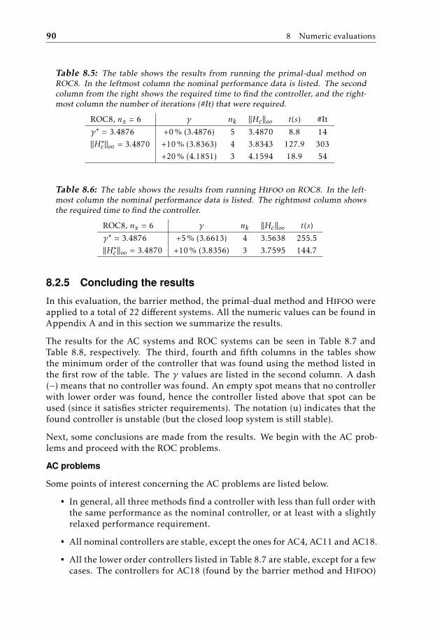
90 8 Numeric evaluations
Table 8.5: The table shows the results from running the primal-dual method onROC8. In the leftmost column the nominal performance data is listed. The secondcolumn from the right shows the required time to find the controller, and the right-most column the number of iterations (#It) that were required.
ROC8, nx = 6 γ nk ||Hc ||∞ t(s) #It
γ∗ = 3.4876 +0 % (3.4876) 5 3.4870 8.8 14||H∗c ||∞ = 3.4870 +10 % (3.8363) 4 3.8343 127.9 303
+20 % (4.1851) 3 4.1594 18.9 54
Table 8.6: The table shows the results from running Hifoo on ROC8. In the left-most column the nominal performance data is listed. The rightmost column showsthe required time to find the controller.
ROC8, nx = 6 γ nk ||Hc ||∞ t(s)
γ∗ = 3.4876 +5 % (3.6613) 4 3.5638 255.5||H∗c ||∞ = 3.4870 +10 % (3.8356) 3 3.7595 144.7
8.2.5 Concluding the results
In this evaluation, the barrier method, the primal-dual method and Hifoo wereapplied to a total of 22 different systems. All the numeric values can be found inAppendix A and in this section we summarize the results.
The results for the AC systems and ROC systems can be seen in Table 8.7 andTable 8.8, respectively. The third, fourth and fifth columns in the tables showthe minimum order of the controller that was found using the method listed inthe first row of the table. The γ values are listed in the second column. A dash(−) means that no controller was found. An empty spot means that no controllerwith lower order was found, hence the controller listed above that spot can beused (since it satisfies stricter requirements). The notation (u) indicates that thefound controller is unstable (but the closed loop system is still stable).
Next, some conclusions are made from the results. We begin with the AC prob-lems and proceed with the ROC problems.
AC problems
Some points of interest concerning the AC problems are listed below.
• In general, all three methods find a controller with less than full order withthe same performance as the nominal controller, or at least with a slightlyrelaxed performance requirement.
• All nominal controllers are stable, except the ones for AC4, AC11 and AC18.
• All the lower order controllers listed in Table 8.7 are stable, except for a fewcases. The controllers for AC18 (found by the barrier method and Hifoo)

8.2 The barrier method and the primal-dual method 91
Table 8.7: The table summarizes the evaluations of all three tested methods on theAC problems. See Section 8.2.5 for details.
System γ Barr.(nk) PD(nk) Hifoo (nk)
AC2, nx=5 +0 % (0.1115) 0 0 0
AC3, nx=5 +0 % (2.9701) 1 1 -+5 % (3.1186) 3
+10 % (3.2671) 2+20 % (3.564) 0 0 1
+50 % (4.4551) 0
AC4, nx=4 +0 % (0.5579) 1 2 2 (u)(u) +5 % (0.5858) 1 1 (u)
AC5, nx=4 +0 % (658.8393) 1 1 -+5 % (691.7813) 0 0 0
AC6, nx=7 +0 % (3.4328) 2 - -+5 % (3.6045) 1 3
+10 % (3.7761) 1+20 % (4.1194) 0 0 0
AC7, nx=9 +0 % (0.0384) 6 - -+5 % (0.0403) 5 2 2
+10 % (0.0422) 3+20 % (0.0461) 2+50 % (0.0576) 1 1
AC8, nx=9 +0 % (1.6220) 3 - 4+5 % (1.7131) 2 5 1
+10 % (1.7842) 1+20 % (1.9464) 1+50 % (2.4330) 0 0 0
AC9, nx=10 +0 % (1.0004) 3 - -+5 % (1.0504) 2 3 0
+10 % (1.1004) 0
AC11, nx=5 +0 % (2.8121) 1 1 -(u) +5 % (2.9527) 0 1 (u)
+50 % (4.2181) 0 0
AC15, nx=4 +0 % (14.8759) 1 1 -+5 % (15.6197) 0 0 0
AC16, nx=4 +0 % (14.8851) 0 0 0
AC17, nx=4 +0 % (6.6125) 0 0 0
AC18, nx=10 +0 % (5.3967) 8 (u) - -(u) +10 % (5.9364) 7 (u)
+20 % (6.4760) 5 (u)+50 % (8.0950) 6 (u) 1 (u)
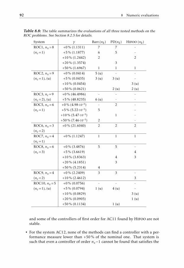
92 8 Numeric evaluations
Table 8.8: The table summarizes the evaluations of all three tested methods on theROC problems. See Section 8.2.5 for details.
System γ Barr.(nk) PD(nk) Hifoo (nk)
ROC1, nx=8 +0 % (1.1311) 7 7 -(nc=1) +5 % (1.1877) 6 5 -
+10 % (1.2442) 2 2+20 % (1.3574) 3+50 % (1.6967) 1 1 1
ROC2, nx=9 +0 % (0.0414) 5 (u) - -(nc=1), (u) +5 % (0.0435) 3 (u) 3 (u) -
+10 % (0.0454) 3 (u)+50 % (0.0621) 2 (u) 2 (u)
ROC3, nc=9 +0 % (46.4986) - - -(nc=2), (u) +5 % (48.8235) 6 (u) - -
ROC5, nx=6 +0 % (4.98·10−5) - 2 -(nc=1) +5 % (5.22·10−5) 5 -
+10 % (5.47·10−5) 1 -+50 % (7.46·10−5) 2 -
ROC6, nx=3 +0 % (21.6040) 2 2 2(nc=2)
ROC7, nx=4 +0 % (1.1247) 1 1 1(nc=1)
ROC8, nx=6 +0 % (3.4876) 5 5 -(nc=3) +5 % (3.6619) 4
+10 % (3.8363) 4 3+20 % (4.1851) 3+50 % (5.2314) 4
ROC9, nx=4 +0 % (2.2409) 3 3 -(nc=2) +10 % (2.4612) 3
ROC10, nx=5 +0 % (0.0756) - - -(nc=1), (u) +5 % (0.0794) 1 (u) 4 (u) -
+10 % (0.0829) 3 (u)+20 % (0.0905) 1 (u)+50 % (0.1134) 1 (u)
and some of the controllers of first order for AC11 found by Hifoo are notstable.
• For the system AC12, none of the methods can find a controller with a per-formance measure lower than +50 % of the nominal one. That system issuch that even a controller of order nx−1 cannot be found that satisfies the
8.2 The barrier method and the primal-dual method 93
constraints.
• For almost all controllers found by the barrier method, the heuristics forfinding the initial point actually finds a solution to the problem. This meansthat Algorithm 8 does not need to run, hence the problem is solved veryfast.
• According to Gumussoy and Overton [2008a], Hifoo is able to find con-trollers for AC10. The barrier method and the primal-dual method cannotfind controllers for AC10, due to large-scale issues.
ROC problems
For the ROC problems, it is worthwhile to point out the following.
• The nominal controllers for ROC2, ROC3 and ROC10 are unstable.
• Neither of the three methods, that are investigated here, manage to finda controller for ROC2 that is stable. The closed loop system is of coursestable, though.
• The barrier method is the only method that finds a controller for ROC3,even though the controller is unstable.
• For ROC5, the barrier method and the primal-dual method find controllersthat are sufficiently good, while Hifoo does not.
• The heuristics used in the barrier method manage to find solutions for manyof the ROC problems, similar as for the AC problems, and hence solvesthese problems very fast.
Quantifying the results
In this section we will attempt to quantify the results by grading the differentmethods. We will take two aspects into account: the ability to find low ordercontrollers with no or little performance loss and the ability to find the lowestorder controller with at most 50 % performance loss. If a method has the bestresult for a system, with respect to one of the criteria above, it will get one point.If several methods have equal result, these methods get one point each. We willbase the grading on Table 8.7 and Table 8.8.
Prioritizing performanceThe grading with respect to performance is done as follows. We look at the +0 %row for each system and give a point to the method that found the lowest ordercontroller. If several methods have the same order, each method gets a point. Ifno method found a controller with +0 % performance loss, continue to +5 %, andso on. For example, all methods get a point for AC2, the barrier and the primal-dual method get points for AC3, but only the barrier method gets a point for AC4.The results from this grading procedure can be seen in Table 8.9. The results areclearly in favor of the barrier method, followed by the primal-dual method andlast, Hifoo.

94 8 Numeric evaluations
Table 8.9: Grading with respect to closed loop performance. See Section 8.2.5 fordetails on the grading procedure.
Method Grade
The barrier method 21The primal-dual method 13Hifoo 5
Prioritizing lowest orderThe grading with performance with respect to lowest order is performed as fol-lows. For each system, we look at the controller with the lowest order, but at thesame time having the least drop in performance. If several methods have foundcontrollers with the same order and performance, each of them get a point. Forexample, for AC7 the primal-dual method and Hifoo get a point each. For AC9,Hifoo gets a point. The results from this grading procedure can be seen in Ta-ble 8.10. The results indicate that all three methods are equally good at findingthe lowest order controllers within +50 % of the nominal peformance.
Table 8.10: Grading with respect to lowest order of the controller. See Section 8.2.5for details on the grading procedure.
Method Grade
The barrier method 15The primal-dual method 16Hifoo 14
8.2.6 Concluding remarks on the evaluation
• For some systems, ROC3 and ROC5, Hifoo cannot find any controllerwithin at least 50 % of the nominal performance, while the barrier methodsucceeds in both cases, and the primal-dual method succeeds in the ROC5case.
• Hifoo has shown to be able to solve problems with large dimensions asreported in Gumussoy and Overton [2008a]. This certainly favors Hifoowhen systems of this kind are addressed.
• The interface for Hifoo is more developed than the interfaces for the bar-rier method and the primal-dual method. Since it is not needed to supply avalue of γ when running, Hifoo certainly has an edge in terms of simplicityfor the user.
• The random elements in Hifoo can cause unexpected and unreliable re-sults. A solution for that is to calculate a large batch of controllers for thesystem to be controlled so that the random elements have less impact onthe results. This, however, requires more computational time.

8.3 The quasi-Newton method 95
• The approach in the barrier method is somewhat ad hoc, but to the authorit is quite remarkable that the performance is as good as it is, compared tothe primal-dual method and Hifoo.
• The framework for the primal-dual method is thoroughly studied in theliterature, so the fact that it performs quite well is not a big surprise.
• The barrier method is the best method at finding lower order controllerswhen performance is prioritized. The primal-dual method is second bestfollowed by Hifoo. This statement is supported by the results in Table 8.9.
• When the aim is to find the lowest order controller that has a closed loopH∞ norm no worse than +50 % of the nominal value, then the conclusionis that the barrier method, the primal-dual method and Hifoo performequally well. This statement is supported by the results in Table 8.10.
This concludes the evaluation of the barrier method and the primal-dual method.
8.3 The quasi-Newton method
In this section we present the evaluation of the quasi-Newton method from Chap-ter 6 that calculates a positive definite approximation of the Hessian by usingdamped BFGS updating.
All experiments in this section were performed on a Dell Optiplex GX620 with2GB RAM, Intel P4 640 (3.2 GHz) CPU running under Windows XP usingMatlab, version 7.4 (R2007a).
8.3.1 Benchmarking problems
We have chosen to evaluate this method on a total of 48 different systems fromthe benchmarking problem library COMPleib with the number of states rangingfrom 4 to 24. These systems are AC1-18, ROC1-10, NN11, REA3, CM1, EB1-4,HE6, HE7, JE2-3, AGS, BDT1, IH, CSE1, TG1, WEC1-3 and DLR1. Some systemsresulted in too complex matrix computations for the quasi-Newton method tohandle and therefore no controller was calculated for these systems. These sys-tems are AC10, AC13-14, and JE2. This results in 44 systems being part of theevaluation.
8.3.2 Evaluated methods
In this evaluation the following methods are compared.
• The quasi-Newton method (QN for short).
• Hifoo 2.0 with Hanso 1.01. For a brief description of Hifoo, see Sec-tion 8.1.2. Both default mode and fast mode are evaluated.

96 8 Numeric evaluations
8.3.3 The tests
The tests were carried out as follows. First, the full order controller (nominalcontroller) was computed. In these computations γ was minimized, which is aconvex problem since there is no rank constraint involved. This controller wascomputed using the Control System Toolbox in Matlab, using the hinfsyn com-mand, with the ’lmi’ option. The minimized upper bound on the performancemeasure obtained using the nominal controller is denoted γ∗ and the achievedclosed loop performance is denoted ‖H ∗c‖∞.
Define a vector of multipliers
γ =(1 1.05 1.1 1.2 1.35 1.5 2 3 5 10
),
where each element in the vector γ refers to different degrees of relaxations of theperformance requirement, i.e. +5 %, +10 %, etc. An increase of the upper boundof the H∞ norm, γ , by more than a factor 10 is considered not to be of any interesthere because the performance we sacrifice then is too much.
The quasi-Newton primal-dual method was applied in order to find reduced or-der controllers with nc ≤ nk ≤ nk,max states, where nc is a lower bound on thenumber of states of the controller required to stabilize the system and wherenk,max = min(10, nx−1). Let γ = γ∗γi , where 1 ≤ i ≤ 10 is the index of the vectorγ and i = 1 at start. This procedure is described by Algorithm 10.
Algorithm 10 An algorithm for iterating through orders and performance
Calculate nominal controller and calculate γ∗ = ‖H ∗c‖∞.Set i := 1, nk := min(10, nx−1).while nk ≥ nc and i ≤ 10 do
Apply the QN algorithm using γ = γ∗γnif success, save controller, set nk := nk−1else, set i := i+1end if
end while
If the QN algorithm is successful, a controller of a lower order is found. If not,the performance requirement is relaxed (i is increased). Note however that theabove algorithm of iterating through orders and performance is just one way ofevaluating the QN algorithm, and that no initial controller is needed to run thealgorithm, just a value of γ .
The evaluation of Hifoo was performed as follows. For each system, controllersof orders from nk,max down to nc were searched for. For each order, Hifoo wasapplied ten times and the closed loop H∞ norm and the computational timewas saved for each run. The reason for applying it ten times is explained inSection 8.1.2.
The minimum and median H∞ norm that was achieved by Hifoo for each systemand controller order (nk) was calculated. These are denoted min and med. The as-

8.3 The quasi-Newton method 97
sociated required computational time is sum of the required time for all ten runs,while for the median H∞ norm the mean time of these ten runs are calculated.
The required time for the algorithms to run was computed using the commandcputime. Using the command norm(Gc,inf,1e-6) the H∞ norm was com-puted, where Gc is the closed loop system and the third argument is the toleranceused in the calculations. Note that we take all the time needed into account, evenQN runs that fail to find a controller.
Remark 8.2. In contrast to the evaluation of the barrier method and the primal-dualmethod in Section 8.2.3, this way of evaluating the methods may favor Hifoo. The reasonis that the quasi-Newton method is now applied without any knowledge of the closed loopH∞ norm that may be achieved. In order to even out the odds somewhat, we tolerate ahigher level of relaxation of the performance requirement in this evaluation compared tothe evaluation in Section 8.2. However, in cases where the closed loop H∞ norm when us-ing a reduced order controller is close to the closed loop H∞ norm when using a full-ordercontroller it may instead favor the quasi-Newton method. Though, without any knowl-edge of the system it is impossible to draw any conclusions regarding this issue.
8.3.4 A case study, AC6
For the system AC6 with seven states (nx = 7), the closed loop H∞ norms arelisted in Table 8.11. The time required to compute the results was 218 s usingthe QN algorithm and 50033 s using Hifoo in default mode, i.e., almost a factorof 230. When using Hifoo in fast mode, the required time is 8221 s, i.e. almosta factor of 38 compared to QN. Figure 8.1 and Figure 8.2 illustrate the achievednorms for the system AC6 using Hifoo default mode and fast mode, respectively.
In Table 8.11 we can see that the minimum values from Hifoo are lower thanthose from QN in 3 out of 7 cases, while ending in a draw in 3 cases resulting ina win ratio of 64 % for Hifoo and 36 % for QN. However, if we use the medianvalues, the win ratio is only 43 % for Hifoo, but then the time required should bedivided by 10, resulting in a factor ≈ 4 in time compared to QN. For Hifoo fastmode the H∞ norms are higher in general as expected, but for nk = 2 the normis actually lower than what is achieved when using default mode, which is theresult of the nonconvexity of the problem combined with the nondeterministicbehavior of Hifoo.
In Appendix B an extract from Ankelhed et al. [2010] is presented. It shows de-tailed results from the evaluation of the quasi-Newton method and Hifoo, nor-mal mode for the system AC6.
8.3.5 Extensive study
The quasi-Newton algorithm, Hifoo default and fast modes were applied to atotal of 44 systems, as mentioned in Section 8.3.1. Note that the same tuningparameters in the quasi-Newton algorithm were used for all systems in the study,i.e., no individual tuning for different systems was done.
For each system in this study the win percent values were calculated and aver-

98 8 Numeric evaluations
0 1 2 3 4 5 6 73.4
3.5
3.6
3.7
3.8
3.9
4
4.1
4.2
nk: number of states
||H
c|| ∞
Compleib system AC6
QNHifoo.medHifoo.minNom. H∞
Figure 8.1: The plot shows the closed loop H∞ norm for the quasi-Newton method (QN) algorithm and Hifoo default mode, when applied toCOMPleib system AC6.
0 1 2 3 4 5 6 73.4
3.5
3.6
3.7
3.8
3.9
4
4.1
4.2
nk: number of states
||H
c|| ∞
Compleib system AC6
QNHifoo.medHifoo.minNom. H∞
Figure 8.2: The plot shows the closed loop H∞ norm for the quasi-Newtonmethod (QN) algorithm and Hifoo fast mode, when applied to COMPleibsystem AC6.

8.3 The quasi-Newton method 99
aged over all systems. In cases where the quasi-Newton algorithm cannot find acontroller but Hifoo can, it was assumed a win for the latter. If the difference innorm obtained by the different methods was less than 1% it was declared a draw,so that minor numerical differences are not a big factor in the results. Also, anycalculated controller that resulted in an unstable closed loop system, regardlessof the used method, was counted as a failure.
The results from applying the algorithms on all 44 systems used in the evalua-tion can be seen in Ankelhed et al. [2010], but are summarized in Table 8.12 andTable 8.13. We can see that the default mode of Hifoo is better than the quasi-Newton algorithm in 61 % of the cases when the minimum H∞ norm of the tenruns are chosen, but the required time is more than a factor of 17 of what is re-quired by the quasi-Newton algorithm. However, if we compare the median H∞norm of the ten runs instead, the number is only 55 % of the cases but the re-quired time is now approximately 1.7 times more compared to the quasi-Newtonalgorithm.
As for the fast mode option of Hifoo, the required time is about a quarter neededcompared to the default mode, but the difference in the results is quite small. Thebest achieved norm is approximately the same but the median values are better.
Table 8.11: Results from computing controllers for the COMPleib system AC6 with7 states. The best results (within an interval of 1 % of the best value if there are severalclose to each other) for each controller order are marked with bold font. Requiredcomputational time is 218 s for the quasi-Newton method (QN), 50033 s for Hifoodefault mode and 8221 s for Hifoo fast mode.
Hifoo, Default mode Hifoo, Fast mode
nk QN, ‖H‖∞ ‖H‖med∞ ‖H‖min
∞ ‖H‖med∞ ‖H‖min
∞6 3.4325 3.5301 3.4967 3.6132 3.55195 3.4328 3.5349 3.4481 3.6119 3.54444 3.5944 3.5602 3.5019 3.6709 3.62733 3.5948 3.5851 3.5069 3.7186 3.55392 3.5831 3.5960 3.5725 3.7023 3.56011 3.7649 3.6438 3.5859 3.7863 3.67720 4.1189 4.1140 4.1140 4.1140 4.1140
Table 8.12: Summary for all systems when comparing the quasi-Newton method(QN) and Hifoo, default mode. More details can be found in Section 8.3.5.
QN Hifoo, min Hifoo, med
Average win, min 39 % 61 % -Average win, med 45 % - 55 %Time required 8.25 · 104 s 1.44 · 106 s 1.44 · 105 s
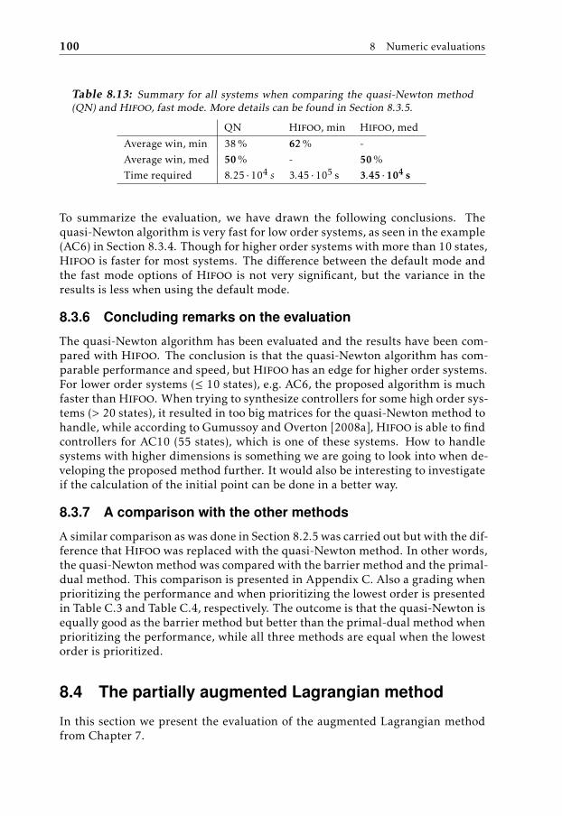
100 8 Numeric evaluations
Table 8.13: Summary for all systems when comparing the quasi-Newton method(QN) and Hifoo, fast mode. More details can be found in Section 8.3.5.
QN Hifoo, min Hifoo, med
Average win, min 38 % 62 % -Average win, med 50 % - 50 %Time required 8.25 · 104 s 3.45 · 105 s 3.45 · 104 s
To summarize the evaluation, we have drawn the following conclusions. Thequasi-Newton algorithm is very fast for low order systems, as seen in the example(AC6) in Section 8.3.4. Though for higher order systems with more than 10 states,Hifoo is faster for most systems. The difference between the default mode andthe fast mode options of Hifoo is not very significant, but the variance in theresults is less when using the default mode.
8.3.6 Concluding remarks on the evaluation
The quasi-Newton algorithm has been evaluated and the results have been com-pared with Hifoo. The conclusion is that the quasi-Newton algorithm has com-parable performance and speed, but Hifoo has an edge for higher order systems.For lower order systems (≤ 10 states), e.g. AC6, the proposed algorithm is muchfaster than Hifoo. When trying to synthesize controllers for some high order sys-tems (> 20 states), it resulted in too big matrices for the quasi-Newton method tohandle, while according to Gumussoy and Overton [2008a], Hifoo is able to findcontrollers for AC10 (55 states), which is one of these systems. How to handlesystems with higher dimensions is something we are going to look into when de-veloping the proposed method further. It would also be interesting to investigateif the calculation of the initial point can be done in a better way.
8.3.7 A comparison with the other methods
A similar comparison as was done in Section 8.2.5 was carried out but with the dif-ference that Hifoo was replaced with the quasi-Newton method. In other words,the quasi-Newton method was compared with the barrier method and the primal-dual method. This comparison is presented in Appendix C. Also a grading whenprioritizing the performance and when prioritizing the lowest order is presentedin Table C.3 and Table C.4, respectively. The outcome is that the quasi-Newton isequally good as the barrier method but better than the primal-dual method whenprioritizing the performance, while all three methods are equal when the lowestorder is prioritized.
8.4 The partially augmented Lagrangian method
In this section we present the evaluation of the augmented Lagrangian methodfrom Chapter 7.
8.4 The partially augmented Lagrangian method 101
All experiments were performed on a DellOptiplexGX620 with 2GB RAM, In-tel P4 640 (3.2 GHz) CPU running under Windows XP using Matlab, version7.11 (R2010b).
8.4.1 Benchmarking problems
A collection of systems with different number of states ranging from 4 to 24 werechosen from the benchmarking library COMPleib. These are AC2, AC5, AC18,CM1, EB4, JE3 and IH.
8.4.2 Evaluated methods
In this evaluation the following methods are compared.
• The augmented Lagrangian method.
• Hifoo 3.0 with Hanso 2.0.
• Hinfstruct (from Matlab version 7.11).
For a brief description of Hifoo and Hinfstruct, see Section 8.1.
8.4.3 The tests
Since all methods in this evaluation attempts to minimize the closed loop H∞norm in the optimization while searching for a stabilizing controller, the evalua-tion procedure in this section is quite straight-forward. Next, the obtained closedloop H∞ norms and required computational times are compared.
The results from the evaluation is presented in Table 8.14, where the H∞ normsand required computational times for the respective methods are displayed. Notethat the same settings were used throughout the whole evaluation for the aug-mented Lagrangian method. Cases where the augmented Lagrangian methodhad numerical problems are marked by ∗. Hifoo was run ten times for everycombination of system and controller order using the default settings. The rea-son for applying it ten times is explained in Section 8.1.2. The best H∞ normfrom these ten runs is displayed in Table 8.14 while the required time is the sumof all ten runs. The options for Hinfstruct were modified in order to add twoextra randomized starting points for reasons that are explained in Section 8.1.3.
The upper part of Table 8.14 shows the results from when controllers of eitherorder zero or three were synthesized in order to evaluate both static output feed-back controllers and reduced order feedback controllers. In cases where only thestatic output feedback controller is shown it is due to the fact that the higher or-der controllers turned out to have the same performance, thus there is no gain inusing these results.
Since the computational complexity of Hifoo and Hinfstruct depend on thenumber of parameters in the controller while the augmented Lagrangian methoddoes not, we chose to also include a system (IH) which has 11 input signals and10 output signals in order to check if the results would differ. The number of

102 8 Numeric evaluations
decision variables for Hinfstruct and Hifoo is n2k + nkny + nunk + nuny while
for the augmented Lagrangian method it is nx(nx + 1) + 1, which means that thenumber of decision variables in our method is not affected by the number ofstates of the controller (nk), inputs (nu) or outputs (ny), while the other methodsare. The results of this evaluation are shown in the lower part of Table 8.14. Forthis example we also synthesized controllers of higher order than for the otherexamples.
As comparison we also included the results from the quasi-Newton method inTable 8.14. These results are taken from Ankelhed et al. [2010].
Table 8.14: Results from evaluation on a collection of systems from COMPleib.The first column displays the system name, the order of the system, the number ofinputs and outputs and the order of the controller that was synthesized. The sec-ond, third, forth and fifth columns show the H∞ norm and required time for theaugmented Lagrangian method (AL), Hinfstruct (HS), Hifoo (HF) and the quasi-Newton method (QN) respectively. Cases where the augmented Lagrangian methodhad numerical problems are marked by ∗.
Sys, (nx,nu ,ny ,nk) ‖ · ‖AL∞ , tAL ‖ · ‖HS
∞ , tHS ‖ · ‖HF∞ , tHF ‖ · ‖QN
∞ , tQN
AC2 (5,3,3,0) 0.11, 19.1 s 0.11, 3.47 s 0.11, 168 s 0.11, 2.89 sAC5 (4,2,2,0) 670, 20.8 s 665, 1.80 s 669, 24.8 s 691, 3.81 sAC5 (4,2,2,3) 660∗, 10.3 s 658, 3.88 s 643, 1100 s 664, 3.70 sAC18 (10,2,2,0) 14.8, 37.4 s 10.7, 2.97 s 12.6, 124 s Fail, -AC18 (10,2,2,3) 8.09, 36.9 s 6.51, 8.22 s 6.54, 3860 s 18.4, 13.9 sCM1 (20,1,2,0) 0.84, 278 s 0.82, 1.91 s 0.82, 125 s 0.82, 142 sEB4 (20,1,1,0) 2.46∗, 460 s 2.06, 3.94 s 2.06, 10.5 s 2.32, 647 sEB4 (20,1,1,3) 2.14, 370 s 1.82, 7.78 s 1.82, 1160 s 2.05, 192 sJE3 (24,3,6,0) 8.74, 645 s 5.10, 5.31 s 5.10, 4880 s 9.62, 1080 sJE3 (24,3,6,3) 2.89∗, 1403 s 2.90, 11.6 s 2.89, 5910 s 3.11, 1210 s
IH (21,11,10,0) 1.88, 367 s 1.59, 38.0 s 1.90, 2450 s 0.00045, 255 sIH (21,11,10,1) 1.86, 523 s 1.80, 43.0 s 1.80, 2410 s 0.00058, 288 sIH (21,11,10,3) 1.49, 373 s 1.57, 51.0 s 1.74, 2170 s 0.00018, 386 sIH (21,11,10,5) 1.39∗, 868 s 1.15, 65.3 s 1.69, 2620 s 0.00021, 374 sIH (21,11,10,7) 1.61∗, 169 s 0.79, 86.2 s 1.72, 2450 s 0.00023, 1030 s
8.4.4 Results and conclusions
The results in the upper part of Table 8.14 indicate that the augmented Lagrang-ian method achieves comparable results in most cases. However Hinfstructobtains the best results overall and is by far the fastest algorithm. However itdoes not always find the best result of the three methods. Hifoo achieves goodresults, but it requires a lot of computational time.
The results in the lower part of Table 8.14 shows that even if the number of pa-rameters in the controller are many, Hinfstruct achieves better results than the
8.4 The partially augmented Lagrangian method 103
augmented Lagrangian method in all cases but one. For these problems Hifoodoes not perform as well as for the problems in the upper part of the table andthe required time is far more than required by the other methods. However, iftime is an issue, either using fast mode or just running it once would reduce therequired computational time.
The remarkable point for the results regarding the system IH, is that the quasi-Newton method finds controllers in all cases that obtains a closed loop H∞ normthat is almost zero, e.g. 0.00045 for the controller with zero states. In this casethis can be explained by the fact that the full order controller has an H∞ normthat is almost zero. Since the quasi-Newton method starts from the performancemeasure obtained using the full order controller and then relaxes it, it tries tofind lower order controllers that, to begin with, has the same H∞ norm. In thiscase there is even a controller with zero states that obtains this H∞ norm. Thiscontroller seem to be very hard to find for the other three methods that attemptsto minimize the H∞ norm during the optimization. This indicates that the quasi-Newton method has an edge in cases where the obtainable H∞ norm for a loworder controller is close to the full order controller.


9Conclusions and further work
In this chapter we present conclusions regarding evaluation of the suggestedmethods together with some concluding remarks. Some directions for future re-search are also suggested.
9.1 Summary
We have developed and implemented three different methods for solving the non-convex problem related to low order H∞ controller synthesis using linear matrixinequalities with a rank constraint.
The approach used in the thesis is based on formulating the rank constraint inthe classical LMI formulation as a rational equation. By using the fact that thequotient in this equation is nonnegative on the feasible set, we can reformulatethis as an optimization problem where a nonconvex rational function is to beminimized over a convex set defined by linear matrix inequalities.
To solve this optimization problem, we have proposed three different methods,namely a barrier method, a primal-dual method and a partially augmented La-grangian method. A slight modification of the primal-dual method resulted in anadditional method called the quasi-Newton method. These methods have beenevaluated on a set of different examples and compared with two methods in theliterature, Hifoo and Hinfstruct.
105

106 9 Conclusions and further work
9.2 Conclusions
The following conclusions can be drawn. These conclusions answer the questionsin Section 1.2.
• The barrier method performs well, at least for systems with 10 states or lessas is seen in the evaluation in Section 8.2.
• The quasi-Newton method has shown to perform well for systems witharound 20 states or less as seen in the evaluation in Section 8.3.
• The quasi-Newton method achieves slightly better performance than theprimal-dual method and has similar performance as the barrier method, asindicated by the comparison in Section 8.3.7. However, the quasi-Newtonmethod requires less computational time than both the other methods.
• The partially augmented Lagrangian method achieves good results for sys-tems of around 25 states or less as seen in the evaluation in Section 8.4. Formost systems this method performs better than the quasi-Newton method.Thus the partially augmented Lagrangian method obtains the best resultsoverall among the suggested methods.
• Under certain circumstances, as for the system IH in Section 8.4, the quasi-Newton method achieves better results than the partially augmented La-grangian method, Hinfstruct and Hifoo.
• The barrier method, the primal-dual method and the quasi-Newton methodrequire an upper bound on the performance, γ , before the algorithms canstart. This is in general a disadvantage compared to the partially augment-ed Lagrangian method, Hifoo and Hinfstruct. To some extent this can bedealt with by using e.g. Algorithm 10 (An algorithm for iterating throughorders and performance).
• All the suggested methods in this thesis use symmetric matrix variablessince their approach is based on Theorem 2.1. The size of these variablesgrows with the square of the order of the system. This fact makes thesemethods less suitable for systems of higher order.
• Methods that do not use approaches involving symmetric matrix variables,like Hifoo and Hinfstruct, seem better fitted for synthesizing low ordercontrollers for systems of very high order. The reason for this is that thenumber of variables in these methods are equal to the number of free pa-rameters in the controller. However, the associated optimization problemsare not only nonconvex, but also nonsmooth and therefore difficult to solve.
• The evaluation in this thesis indicate that Hinfstruct obtains the best re-sults overall, but not in all cases. Hifoo is a good alternative, but may re-quire considerable computational time if it needs to be run 10 times. Theseare two of the best software packages for low order H∞ controller synthesisthat are available.

9.3 Future work 107
9.3 Future work
Since all suggested methods are local methods, the initial point is important forthe performance of the algorithms. It would be interesting to look further intohow to choose the initial point in a better way.
In cases where the barrier method does not find a local minimum and γ needsto be increased, warmstarting procedures could be implemented. Here we coulduse the point at which the algorithm terminated as a starting point in the newproblem since the new problem is merely a relaxation of the previous one.
The impact of using other scaling matrices P for the primal-dual algorithm wouldbe interesting to investigate.
A more efficient algorithm for calculating the derivatives of the coefficients of thecharacteristic polynomial was presented in Ankelhed [2011]. This algorithm wasused together with a modified symmetric indefinite factorization in the partiallyaugmented Lagrangian algorithm. It would be interesting to use this combinationin the barrier method and in the primal-dual method to investigate what resultsthat can be achieved.
The primal-dual method, the quasi-Newton method and the partially augmentedLagrangian method do not use a merit function combined with a line search. Byusing a proper merit function and implementing a line search with step lengthsthat satisfy the Wolfe conditions, better convergence properties of the algorithmscould be obtained, see Nocedal and Wright [2006].
The termination criterion that is used in the partially augmented Lagrangianmethod is ad hoc and could be replaced with a more elaborate one, e.g. the onein Noll et al. [2004].
It would be interesting to apply a trust-region method to the problem formula-tions in e.g. (4.7) and (7.2) and investigate what performance that can be achieved.


Part IV
Tables with additional results
109

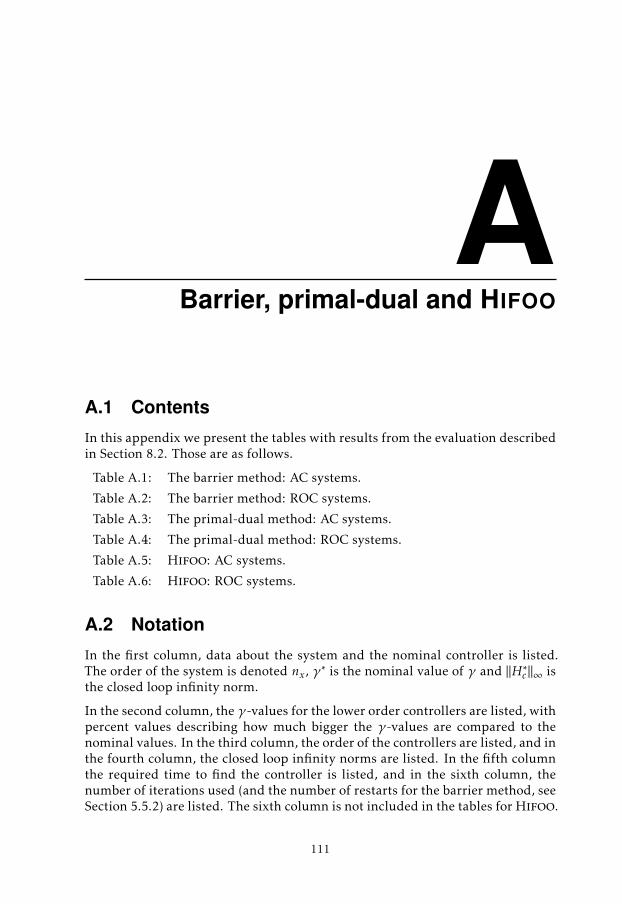
ABarrier, primal-dual and HIFOO
A.1 Contents
In this appendix we present the tables with results from the evaluation describedin Section 8.2. Those are as follows.
Table A.1: The barrier method: AC systems.
Table A.2: The barrier method: ROC systems.
Table A.3: The primal-dual method: AC systems.
Table A.4: The primal-dual method: ROC systems.
Table A.5: Hifoo: AC systems.
Table A.6: Hifoo: ROC systems.
A.2 Notation
In the first column, data about the system and the nominal controller is listed.The order of the system is denoted nx, γ∗ is the nominal value of γ and ‖H ∗c‖∞ isthe closed loop infinity norm.
In the second column, the γ-values for the lower order controllers are listed, withpercent values describing how much bigger the γ-values are compared to thenominal values. In the third column, the order of the controllers are listed, and inthe fourth column, the closed loop infinity norms are listed. In the fifth columnthe required time to find the controller is listed, and in the sixth column, thenumber of iterations used (and the number of restarts for the barrier method, seeSection 5.5.2) are listed. The sixth column is not included in the tables for Hifoo.
111

112 A Barrier, primal-dual and Hifoo
Table A.1: Results from running the barrier method on the AC problems.
AC2, nx = 5 γ nk ||Hc ||∞ t(s) #It(#Rs)γ∗ = 0.1115 +0 % (0.1115) 0 0.1115 1.8 0(0)||H∗c ||∞ = 0.1115
AC3, nx = 5γ∗ = 2.9701 +0 % (2.9701) 1 2.9700 2.2 0(0)||H∗c ||∞ = 2.9601 +20 % (3.5641) 0 3.4783 16.8 338(0)
AC4, nx = 4γ∗ = 0.5579, (u) +0 % (0.5579) 1 0.5577 6.2 69(2)||H∗c ||∞ = 0.5575
AC5, nx = 4γ∗ = 658.8 +0 % (658.8393) 1 658.8390 2.0 0(0)||H∗c ||∞ = 658.2 +5 % (691.7813) 0 666.8880 10.2 277(0)
AC6, nx = 7γ∗ = 3.4328 +0 % (3.4328) 2 3.4328 2.7 0(0)||H∗c ||∞ = 3.4314 +20 % (4.1194) 0 4.1155 68.8 648(0)
AC7, nx = 9γ∗ = 0.0384 +0 % (0.0384) 6 0.0383 3.0 0(0)||H∗c ||∞ = 0.0380 +5 % (0.0403) 5 0.0400 3.0 0(0)
+10 % (0.0422) 3 0.0413 2.6 0(0)+20 % (0.0461) 2 0.437 2.7 0(0)
AC8, nx = 9γ∗ = 1.6220 +0 % (1.6220) 3 1.6216 573.5 432(1)||H∗c ||∞ = 1.6194 +5 % (1.7031) 2 1.6923 618.5 737(1)
+10 % (1.7842) 1 1.7456 107.6 254(1)+50 % (2.4330) 0 2.1088 73.6 331(1)
AC9, nx = 10γ∗ = 1.0004 +0 % (1.0004) 3 1.0004 4.0 0(0)||H∗c ||∞ = 1.0003 +5 % (1.0504) 2 1.0312 3.5 0(0)
AC11, nx = 5γ∗ = 2.8121, (u) +0 % (2.8121) 1 2.8120 2.1 0(0)||H∗c ||∞ = 2.8111 +50 % (4.2181) 0 4.1211 1.6 0(0)
AC15, nx = 4γ∗ = 14.8759 +0 % (14.8759) 1 14.8759 2.0 0(0)||H∗c ||∞ = 14.8714 +5 % (15.6197) 0 15.5977 1.6 0(0)
AC16, nx = 4γ∗ = 14.8851 +0 % (14.8851) 0 14.8849 1.6 0(0)||H∗c ||∞ = 14.8666
AC17, nx = 4γ∗ = 6.6125 +0 % (6.6125) 0 6.6124 1.5 0(0)||H∗c ||∞ = 6.6124
AC18, nx = 10γ∗ = 5.3967, (u) +0 % (5.3967) 8 5.4004, (u) 4.4 0(0)||H∗c ||∞ = 5.3938 +10 % (5.9364) 7 5.9121, (u) 3.6 0(0)
+50 % (8.0950) 6 7.8395, (u) 3.5 0(0)

A.2 Notation 113
Table A.2: Results from running the barrier method on the ROC problems.
ROC1, nx = 8 γ nk ||Hc ||∞ t(s) #It(#Rs)γ∗ = 1.1311 +0 % (1.1311) 7 1.1311 5.6 0(0)||H∗c ||∞ = 1.1304 +5 % (1.1877) 6 1.1686 1.9 0(0)
+10 % (1.2442) 2 1.2440 134.4 276(0)+50 % (1.6967) 1 1.5716 66.9 271(0)
ROC2, nx = 9γ∗ = 0.0414, (u) +0 % (0.0414) 5 0.0413, (u) 2.7 0(0)||H∗c ||∞ = 0.0413 +5 % (0.0435) 3 0.0427, (u) 2.3 0(0)
ROC3, nx = 9γ∗ = 46.4986, (u) +5 % (48.8235) 6 48.7953, (u) 4.5 0(0)||H∗c ||∞ = 46.4906
ROC5, nx = 6γ∗ = 4.98·10−5 +5 % (5.22·10−5) 5 1.85·10−5 20.4 37(1)||H∗c ||∞ = 4.05·10−5 +50 % (7.46·10−5) 2 6.72·10−5 2.5 0(0)
ROC6, nx = 3γ∗ = 21.604 +0 % (21.6040) 2 21.5550 1.4 0(0)||H∗c ||∞ = 21.557
ROC7, nx = 4γ∗ = 1.1247 +0 % (1.1247) 1 1.1247 1.5 0(0)||H∗c ||∞ = 1.1233
ROC8, nx = 6γ∗ = 3.4876 +0 % (3.4876) 5 3.4870 1.7 0(0)||H∗c ||∞ = 3.4870 +50 % (5.2314) 4 5.2291 1.6 0(0)
ROC9, nx = 4γ∗ = 2.2409 +0 % (2.2409) 3 2.2409 1.7 0(0)||H∗c ||∞ = 2.2375
ROC10, nx = 5γ∗ = 0.0756, (u) +5 % (0.0794) 1 0.0791, (u) 2.2 0(0)||H∗c ||∞ = 0.0754

114 A Barrier, primal-dual and Hifoo
Table A.3: Results from running the primal-dual method on the AC problems.
AC2, nx = 5 γ nk ||Hc ||∞ t(s) #Itγ∗ = 0.1115 +0 % (0.1115) 0 0.1115 2.5 11||H∗c ||∞ = 0.1115
AC3, nx = 5γ∗ = 2.9701 +0 % (2.9701) 1 2.9700 7.8 44||H∗c ||∞ = 2.9601 +20 % (3.5641) 0 3.5637 30.7 306
AC4, nx = 4γ∗ = 0.5579, (u) +0 % (0.5579) 2 0.5575 5.5 41||H∗c ||∞ = 0.5575 +5 % (0.5858) 1 0.5844 9.0 108
AC5, nx = 4γ∗ = 658.8 +0 % (658.8393) 1 658.7662 21.7 251||H∗c ||∞ = 658.2 +5 % (691.7813) 0 670.7818 3.1 18
AC6, nx = 7γ∗ = 3.4328 +5 % (3.6045) 1 3.6038 110.3 279||H∗c ||∞ = 3.4314 +20 % (4.1194) 0 4.1161 12.6 33
AC7, nx = 9γ∗ = 0.0384 +5 % (0.0403) 2 0.0400 254.8 245||H∗c ||∞ = 0.0380 +50 % (0.0576) 1 0.0568 87.5 149
AC8, nx = 9γ∗ = 1.6220 +5 % (1.7031) 5 1.6787 354.3 130||H∗c ||∞ = 1.6194 +20 % (1.9464) 1 1.8654 99.2 139
+50 % (2.4330) 0 2.2806 18.4 34
AC9, nx = 10γ∗ = 1.0004 +5 % (1.0504) 3 1.0298 454.9 200||H∗c ||∞ = 1.0003 +10 % (1.1004) 0 1.0954 120.2 185
AC11, nx = 5γ∗ = 2.8121, (u) +0 % (2.8121) 1 2.8120 7.4 56||H∗c ||∞ = 2.8111 +5 % (2.9527) 0 2.9478 3.7 30
AC15, nx = 4γ∗ = 14.8759 +0 % (14.8759) 1 14.8758 3.9 34||H∗c ||∞ = 14.8714 +5 % (15.6197) 0 15.5450 2.8 26
AC16, nx = 4γ∗ = 14.8851 +0 % (14.8851) 0 14.8849 2.5 23||H∗c ||∞ = 14.8666
AC17, nx = 4γ∗ = 6.6125 +0 % (6.6125) 0 6.6124 2.2 13||H∗c ||∞ = 6.6124
AC18, nx = 10γ∗ = 5.3967, (u) - - - - -||H∗c ||∞ = 5.3938
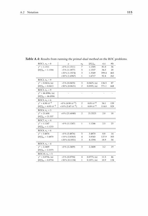
A.2 Notation 115
Table A.4: Results from running the primal-dual method on the ROC problems.
ROC1, nx = 8 γ nk ||Hc ||∞ t(s) #Itγ∗ = 1.1311 +0 % (1.1311) 7 1.1305 81.0 36||H∗c ||∞ = 1.1304 +5 % (1.1877) 5 1.1537 34.3 20
+20 % (1.3574) 3 1.3549 399.4 465+50 % (1.6967) 1 1.6717 92.4 262
ROC2, nx = 9γ∗ = 0.0414, (u) +5 % (0.0435) 3 0.0425, (u) 136.5 87||H∗c ||∞ = 0.0413 +50 % (0.0621) 2 0.0595, (u) 771.1 668
ROC3, nx = 9γ∗ = 46.4986, (u) - - - - -||H∗c ||∞ = 46.4906
ROC5, nx = 6γ∗ = 4.98·10−5 +0 % (4.98·10−5) 2 8.85·10−6 34.1 159||H∗c ||∞ = 4.05·10−5 +10 % (5.47·10−5) 1 8.89·10−6 114.0 929
ROC6, nx = 3γ∗ = 21.604 +0 % (21.6040) 2 21.5523 2.0 18||H∗c ||∞ = 21.557
ROC7, nx = 4γ∗ = 1.1247 +0 % (1.1247) 1 1.1246 2.5 23||H∗c ||∞ = 1.1233
ROC8, nx = 6γ∗ = 3.4876 +0 % (3.4876) 5 3.4870 8.8 14||H∗c ||∞ = 3.4870 +10 % (3.8363) 4 3.8343 127.9 303
+20 % (4.1851) 3 4.1594 18.9 54
ROC9, nx = 4γ∗ = 2.2409 +0 % (2.2409) 3 2.2408 3.2 19||H∗c ||∞ = 2.2375
ROC10, nx = 5γ∗ = 0.0756, (u) +5 % (0.0794) 4 0.0775, (u) 11.5 46||H∗c ||∞ = 0.0754 +50 % (0.1134) 1 0.1071, (u) 10.9 134

116 A Barrier, primal-dual and Hifoo
Table A.5: Results from running Hifoo on the AC examples.
AC2, nx = 5 γ nk ||Hc ||∞ t(s)γ∗ = 0.1115 +0 % (0.1115) 0 0.1115 5.2||H∗c ||∞ = 0.1115
AC3, nx = 5γ∗ = 2.9701 +5 % (3.1186) 3 3.0373 197.3||H∗c ||∞ = 2.9601 +10 % (3.2671) 2 3.2199 141.1
+20 % (3.5641) 1 3.4331 38.7+50 % (4.4551) 0 3.6535 22.8
AC4, nx = 4γ∗ = 0.5579, (u) +0 % (0.5579) 2 0.5573, (u) 37.8||H∗c ||∞ = 0.5575 +5 % (0.5858) 1 0.5589, (u) 33.0
AC5, nx = 4γ∗ = 658.8393 +5 % (691.7813) 0 689.7123 1.2||H∗c ||∞ = 658.2496
AC6, nx = 7γ∗ = 3.4328 +5 % (3.6045) 3 3.5783 441.1||H∗c ||∞ = 3.4314 +10 % (3.7761) 1 3.6610 265.3
+20 % (4.1194) 0 4.1140 67.9
AC7, nx = 9γ∗ = 0.0384 +5 % (0.0403) 2 0.0400 71.0||H∗c ||∞ = 0.0380 +50 % (0.0576) 1 0.0525 18.5
AC8, nx = 9γ∗ = 1.6220 +0 % (1.6220) 4 1.6202 429.3||H∗c ||∞ = 1.6194 +5 % (1.7031) 1 1.6516 130.2
+50 % (2.4330) 0 2.0050 30.4
AC9, nx = 10γ∗ = 1.0004 +5 % (1.0504) 0 1.0054 150.8||H∗c ||∞ = 1.0003
AC11, nx = 5γ∗ = 2.8121, (u) +5 % (2.9527) 1 2.8281, (u) 89.1||H∗c ||∞ = 2.8111 +50 % (4.2181) 0 3.5283 14.2
AC15, nx = 4γ∗ = 14.8759 +5 % (15.6197) 0 15.1702 35.9||H∗c ||∞ = 14.8714
AC16, nx = 4γ∗ = 14.8851 +0 % (14.8851) 0 14.8728 15.4||H∗c ||∞ = 14.8666
AC17, nx = 4γ∗ = 6.6125 +0 % (6.6125) 0 6.6124 0.8||H∗c ||∞ = 6.6124
AC18, nx = 10γ∗ = 5.3967, (u) +20 % (6.4760) 5 6.4722, (u) 385.2||H∗c ||∞ = 5.3938 +50 % (8.0950) 1 7.7691, (u) 48.2

A.2 Notation 117
Table A.6: Results from running Hifoo on the ROC examples.
ROC1, nx = 8 γ nk ||Hc ||∞ t(s)γ∗ = 1.1311 +10 % (1.2442) 2 1.2438 56.1||H∗c ||∞ = 1.1304 +50 % (1.6967) 1 1.4256 21.3
ROC2, nx = 9γ∗ = 0.0414, (u) +10 % (0.0455) 3 0.0448, (u) 310.4||H∗c ||∞ = 0.0413 +50 % (0.0621) 2 0.0506, (u) 147.2
ROC3, nx = 9γ∗ = 46.4986, (u) - - - -||H∗c ||∞ = 46.4906
ROC5, nx = 6γ∗ = 4.98·10−5 - - - -||H∗c ||∞ = 4.05·10−5
ROC6, nx = 3γ∗ = 21.604 +0 % (21.6040) 2 21.5437 62.0||H∗c ||∞ = 21.557
ROC7, nx = 4γ∗ = 1.1247 +0 % (1.1247) 1 1.1224 18.0||H∗c ||∞ = 1.1233
ROC8, nx = 6γ∗ = 3.4876 +5 % (3.6619) 4 3.5638 255.5||H∗c ||∞ = 3.4870 +10 % (3.8363) 3 3.7595 144.7
ROC9, nx = 4γ∗ = 2.2409 +10 % (2.4649) 3 2.4175 162.9||H∗c ||∞ = 2.2375
ROC10, nx = 5γ∗ = 0.0756, (u) +10 % (0.0832) 3 0.0826, (u) 62.7||H∗c ||∞ = 0.0754 +20 % (0.0907) 1 0.0878, (u) 31.0

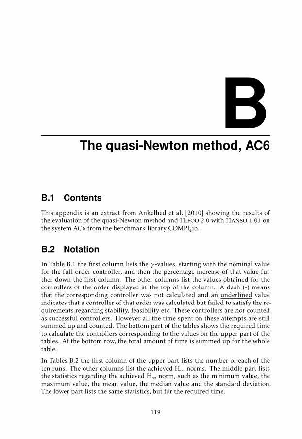
BThe quasi-Newton method, AC6
B.1 Contents
This appendix is an extract from Ankelhed et al. [2010] showing the results ofthe evaluation of the quasi-Newton method and Hifoo 2.0 with Hanso 1.01 onthe system AC6 from the benchmark library COMPleib.
B.2 Notation
In Table B.1 the first column lists the γ-values, starting with the nominal valuefor the full order controller, and then the percentage increase of that value fur-ther down the first column. The other columns list the values obtained for thecontrollers of the order displayed at the top of the column. A dash (-) meansthat the corresponding controller was not calculated and an underlined valueindicates that a controller of that order was calculated but failed to satisfy the re-quirements regarding stability, feasibility etc. These controllers are not countedas successful controllers. However all the time spent on these attempts are stillsummed up and counted. The bottom part of the tables shows the required timeto calculate the controllers corresponding to the values on the upper part of thetables. At the bottom row, the total amount of time is summed up for the wholetable.
In Tables B.2 the first column of the upper part lists the number of each of theten runs. The other columns list the achieved H∞ norms. The middle part liststhe statistics regarding the achieved H∞ norm, such as the minimum value, themaximum value, the mean value, the median value and the standard deviation.The lower part lists the same statistics, but for the required time.
119

120 B The quasi-Newton method, AC6
Table B.1: The table shows the results obtained when applying the quasi-Newtonmethod on COMPleib system AC6, 7 states.
γ / k 6 5 4 3 2 1 03.433 3.432 3.433 2.795·101 - - - -+5% - - 3.594 3.595 3.583 3.687 -+10% - - - - - 3.765 4.891+20% - - - - - - 4.119
t [s]+0% 3.652·101 3.497·101 3.456·101
+5% 8.422 1.019·101 9.078 3.217·101
+10% 8.594 3.208·101
+20% 1.163·101
Total: 2.182·102s
Table B.2: The table shows the results obtained when applying Hifoo, normalmode on COMPleib system AC6, 7 states.
Run / k 6 5 4 3 2 1 01 3.525 3.533 3.545 3.567 3.579 3.600 4.1142 3.516 3.556 3.544 3.604 3.585 3.658 4.1143 3.549 3.563 3.568 3.507 3.759 3.653 4.1144 3.528 3.597 3.564 3.541 3.573 3.586 4.1145 3.533 3.555 3.502 3.812 3.601 3.649 4.1146 3.577 3.519 3.685 3.596 3.699 3.753 4.1147 3.507 3.479 3.568 3.575 3.582 3.638 4.1148 3.497 3.537 3.529 3.596 3.591 3.804 4.1149 3.551 3.448 3.556 3.599 3.658 3.612 4.11410 3.544 3.528 3.633 3.546 3.630 3.616 4.114min 3.497 3.448 3.502 3.507 3.573 3.586 4.114max 3.577 3.597 3.685 3.812 3.759 3.804 4.114mean 3.533 3.532 3.569 3.594 3.626 3.657 4.114med 3.530 3.535 3.560 3.585 3.596 3.644 4.114std 2.371·10−2 4.260·10−2 5.271·10−2 8.275·10−2 6.186·10−2 6.934·10−2 4.296·10−5
t [s]tmin 1.249·103 8.141·102 8.086·102 6.695·102 3.620·102 3.883·102 5.470·101
tmax 1.408·103 1.143·103 9.928·102 7.649·102 5.868·102 4.810·102 1.662·102
tmean 1.337·103 1.030·103 8.704·102 7.095·102 5.198·102 4.350·102 1.018·102
tmed 1.331·103 1.049·103 8.599·102 7.020·102 5.336·102 4.358·102 9.108·101
tstd 4.916·101 8.688·101 4.849·101 3.042·101 6.350·101 2.893·101 3.691·101
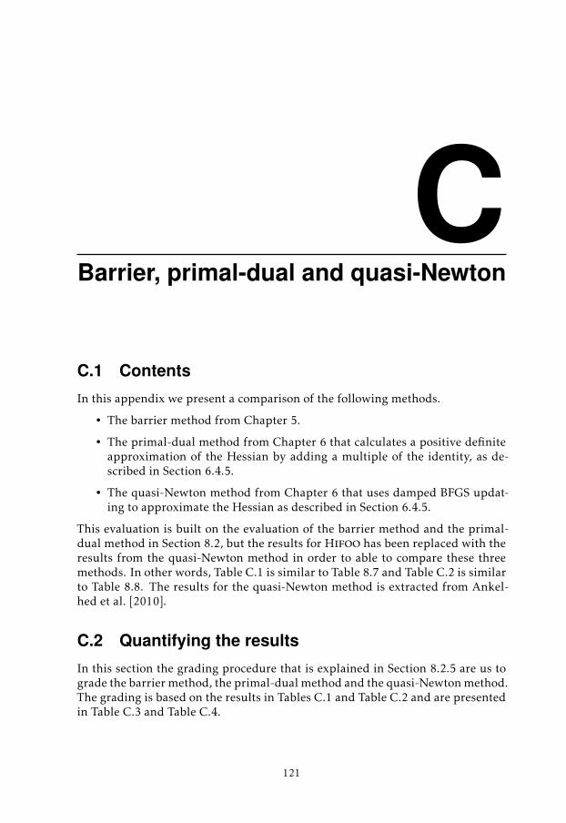
CBarrier, primal-dual and quasi-Newton
C.1 Contents
In this appendix we present a comparison of the following methods.
• The barrier method from Chapter 5.
• The primal-dual method from Chapter 6 that calculates a positive definiteapproximation of the Hessian by adding a multiple of the identity, as de-scribed in Section 6.4.5.
• The quasi-Newton method from Chapter 6 that uses damped BFGS updat-ing to approximate the Hessian as described in Section 6.4.5.
This evaluation is built on the evaluation of the barrier method and the primal-dual method in Section 8.2, but the results for Hifoo has been replaced with theresults from the quasi-Newton method in order to able to compare these threemethods. In other words, Table C.1 is similar to Table 8.7 and Table C.2 is similarto Table 8.8. The results for the quasi-Newton method is extracted from Ankel-hed et al. [2010].
C.2 Quantifying the results
In this section the grading procedure that is explained in Section 8.2.5 are us tograde the barrier method, the primal-dual method and the quasi-Newton method.The grading is based on the results in Tables C.1 and Table C.2 and are presentedin Table C.3 and Table C.4.
121
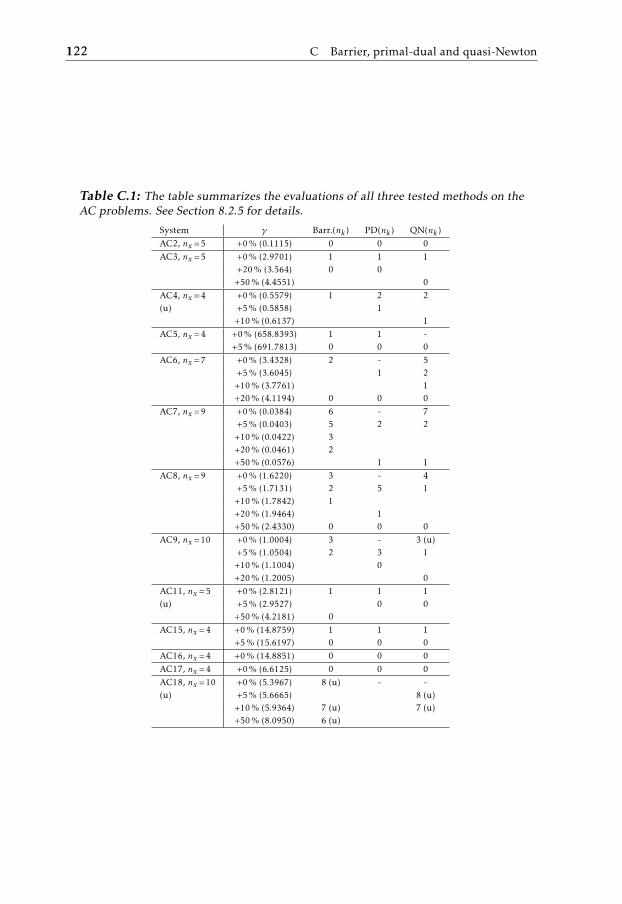
122 C Barrier, primal-dual and quasi-Newton
Table C.1: The table summarizes the evaluations of all three tested methods on theAC problems. See Section 8.2.5 for details.
System γ Barr.(nk ) PD(nk ) QN(nk )AC2, nx =5 +0 % (0.1115) 0 0 0AC3, nx =5 +0 % (2.9701) 1 1 1
+20 % (3.564) 0 0+50 % (4.4551) 0
AC4, nx =4 +0 % (0.5579) 1 2 2(u) +5 % (0.5858) 1
+10 % (0.6137) 1AC5, nx =4 +0 % (658.8393) 1 1 -
+5 % (691.7813) 0 0 0AC6, nx =7 +0 % (3.4328) 2 - 5
+5 % (3.6045) 1 2+10 % (3.7761) 1+20 % (4.1194) 0 0 0
AC7, nx =9 +0 % (0.0384) 6 - 7+5 % (0.0403) 5 2 2
+10 % (0.0422) 3+20 % (0.0461) 2+50 % (0.0576) 1 1
AC8, nx =9 +0 % (1.6220) 3 - 4+5 % (1.7131) 2 5 1
+10 % (1.7842) 1+20 % (1.9464) 1+50 % (2.4330) 0 0 0
AC9, nx =10 +0 % (1.0004) 3 - 3 (u)+5 % (1.0504) 2 3 1
+10 % (1.1004) 0+20 % (1.2005) 0
AC11, nx =5 +0 % (2.8121) 1 1 1(u) +5 % (2.9527) 0 0
+50 % (4.2181) 0AC15, nx =4 +0 % (14.8759) 1 1 1
+5 % (15.6197) 0 0 0AC16, nx =4 +0 % (14.8851) 0 0 0AC17, nx =4 +0 % (6.6125) 0 0 0AC18, nx =10 +0 % (5.3967) 8 (u) - -(u) +5 % (5.6665) 8 (u)
+10 % (5.9364) 7 (u) 7 (u)+50 % (8.0950) 6 (u)

C.2 Quantifying the results 123
Table C.2: The table summarizes the evaluations of all three tested methods on theROC problems. See Section 8.2.5 for details.
System γ Barr.(nk ) PD(nk ) QN(nk )ROC1, nx =8 +0 % (1.1311) 7 7 6(nc =1) +5 % (1.1877) 6 5 5
+10 % (1.2442) 2 4+20 % (1.3574) 3 2+50 % (1.6967) 1 1
ROC2, nx =9 +0 % (0.0414) 5 (u) - 4 (u)(nc =1), (u) +5 % (0.0435) 3 (u) 3 (u) 3 (u)
+50 % (0.0621) 2 (u) 2 (u)ROC3, nc =9 +0 % (46.4986) - - -(nc =2), (u) +5 % (48.8235) 6 (u) - 6 (u)ROC5, nx =6 +0 % (4.98·10−5) - 2 1(nc =1) +5 % (5.22·10−5) 5
+10 % (5.47·10−5) 1+50 % (7.46·10−5) 2
ROC6, nx =3 +0 % (21.6040) 2 2 2(nc =2)ROC7, nx =4 +0 % (1.1247) 1 1 1(nc =1)ROC8, nx =6 +0 % (3.4876) 5 5 5(nc =3) +10 % (3.8363) 4
+20 % (4.1851) 3 3+50 % (5.2314) 4
ROC9, nx =4 +0 % (2.2409) 3 3 3(nc =2)ROC10, nx =5 +0 % (0.0756) - - 1 (u)(nc =1), (u) +5 % (0.0794) 1 (u) 4 (u)
+50 % (0.1134) 1 (u)
Table C.3: Grading with respect to closed loop performance. See Section 8.2.5 fordetails on the grading procedure.
Method GradeThe barrier method 18The primal-dual method 11The quasi-Newton method 16
Table C.4: Grading with respect to lowest order of the controller. See Section 8.2.5for details on the grading procedure.
Method GradeThe barrier method 15The primal-dual method 17The quasi-Newton method 17

124 C Barrier, primal-dual and quasi-Newton
Bibliography
F. Alizadeh, J.A. Haeberly, and M.L. Overton. Primal-dual interior-point meth-ods for semidefinite programming: Convergence rates, stability and numericalresults. SIAM Journal on Optimization, 8(3):746–768, 1998. ISSN 1052-6234.Cited on page 65.
D. Ankelhed. On low order controller synthesis using rational constraints. Licen-tiate thesis no. 1398, Department of Electrical Engineering, Linköping Univer-sity, SE-581 83 Linköping, Sweden, Mar 2009. Cited on page 8.
D. Ankelhed. An efficient implementation of gradient and Hessian calcula-tions of the coefficients of the characteristic polynomial of I - XY. Techni-cal Report LiTH-ISY-R-2997, Department of Automatic Control, Linköpinguniversity, Sweden, 2011. URL http://www.control.isy.liu.se/publications/doc?id=2387. Cited on pages 8, 9, 45, and 107.
D. Ankelhed, A. Helmersson, and A. Hansson. Suboptimal model reduc-tion using LMIs with convex constraints. Technical Report LiTH-ISY-R-2759, Department of Electrical Engineering, Linköping University, SE-581 83Linköping, Sweden, Dec 2006. URL http://www.control.isy.liu.se/publications/doc?id=1889. Not cited.
D. Ankelhed, A. Helmersson, and A. Hansson. A primal-dual method for loworder H-infinity controller synthesis. In Proceedings of the 2009 IEEE Con-ference on Decision and Control, Shanghai, China, Dec 2009. Cited on page8.
D. Ankelhed, A. Helmersson, and A. Hansson. Additional numerical results forthe quasi-Newton interior point method for low order H-infinity controllersynthesis. Technical Report LiTH-ISY-R-2964, Department of Automatic Con-trol, Linköping university, Sweden, 2010. URL http://www.control.isy.liu.se/publications/doc?id=2313. Cited on pages 8, 85, 97, 99, 102,119, and 121.
D. Ankelhed, A. Helmersson, and A. Hansson. A quasi-Newton interior point
125

126 Bibliography
method for low order H-infinity controller synthesis. Accepted for publicationin IEEE Transactions on Automatic Control, 2011a. Cited on page 8.
D. Ankelhed, A. Helmersson, and A. Hansson. A partially augmented Lagrangianalgorithm for low order H-infinity controller synthesis using rational con-straints. Submitted to the 2011 IEEE Conference on Decision and Control,December 2011b. Cited on pages 9 and 73.
P. Apkarian. Comparison of HINFSTRUCT Matlab Robust Control ToolboxR2010b and HIFOO 3.0 with HANSO 2.0, 2010. URL http://pierre.apkarian.free.fr/Benchv3.pdf. Cited on page 85.
P. Apkarian. E-mail correspondance, 2011. Cited on page 85.
P. Apkarian and D. Noll. A prototype primal-dual LMI-interior algorithm fornonconvex robust control problems. Technical Report 01-08, Toulouse, 2001.Cited on page 5.
P. Apkarian and D. Noll. Controller design via nonsmooth multidirectionalsearch. SIAM Journal on Control and Optimization, 44(6):1923–1949, 2006a.ISSN 0363-0129. Cited on pages 5 and 47.
P. Apkarian and D. Noll. Nonsmooth H∞ synthesis. IEEE Transactions on Auto-matic Control, 51(1):71–86, 2006b. Cited on pages 5, 6, 7, 46, 47, and 85.
P. Apkarian and H.D. Tuan. Concave programming in control theory. Journal ofGlobal Optimization, 15(4):343–370, 1999. Cited on page 5.
P. Apkarian and H.D. Tuan. Robust control via concave minimization local andglobal algorithms. IEEE Transactions on Automatic Control, 45(2):299–305,2000. ISSN 0018-9286. Cited on page 5.
P. Apkarian, D. Noll, and H.D. Tuan. Fixed-order H-infinity control design via apartially augmented Lagrangian method. International Journal of Robust andNonlinear Control, 13(12):1137–1148, 2003. ISSN 1049-8923. Cited on pages5, 6, 7, 46, 74, and 76.
P. Apkarian, D. Noll, J.-B. Thevenet, and H.D. Tuan. A spectral quadratic-SDPmethod with applications to fixed-order H2 and H∞ synthesis. In Proceed-ings of 2004 5th Asian Control Conference, volume 2, pages 1337–1345, 2004.Cited on pages 5 and 74.
D. Arzelier, G. Deaconu, S. Gumussoy, and D. Henrion. H2 for Hifoo. Submittedto the IFAC World Congress on Automatic control, August 2011. Cited onpages 6 and 85.
A. Ben-Tal and M. Zibulevsky. Penalty/barrier multiplier methods for convexprogramming problems. SIAM Journal on Optimization, 7(2):347–366, 1997.Cited on page 5.
E.B. Beran. Methods for optimization-based fixed-order control design. Ph.D. Dis-

Bibliography 127
sertation, Technical University of Denmark, Denmark, September 1997. Citedon pages 4 and 20.
S.J. Berkowitz. On computing the determinant in small parallel time using asmall number of processors. Information Processing Letters, 18(3):147 – 150,1984. ISSN 0020-0190. Cited on page 43.
D.P. Bertsekas. Constrained optimization and Lagrange multiplier methods. Aca-demic Press, Inc., New York, USA, 1982. ISBN 0-12-093480-9. Cited on page36.
D.P. Bertsekas. Nonlinear programming. Athena Scientific, Belmont, Mas-sachusetts, USA, 1995. ISBN 1-886529-14-0. Cited on pages 26 and 36.
P.T. Boggs and J.W. Tolle. Sequential quadratic programming. Acta Numerica, 4:1–51, 1995. Cited on page 62.
S. Boyd and L. Vandenberghe. Convex optimization. Cambridge University Press,New York, NY, USA, 2004. ISBN 0521833787. Cited on pages 21, 22, 25, 26,30, 51, and 55.
S. Boyd, L. El Ghaoui, E. Feron, and V. Balakrishnan. Linear matrix inequalitiesin system and control theory. SIAM Studies in Applied Mathematics. SIAM,1994. ISBN 0-89871-334-X. Cited on pages 14, 43, and 53.
C. G. Broyden. The convergence of a class of double-rank minimization algo-rithms, parts 1 and 2. IMA Journal of Applied Mathematics, 6(1):76–90 and222–231, 1970. Cited on page 30.
S. Burer and R.D.C. Monteiro. A nonlinear programming algorithm for solv-ing semidefinite programs via low-rank factorization. Mathematical Program-ming, Series B, 95(2):329–357, 2003. Cited on page 62.
J.V. Burke, A.S. Lewis, and M.L. Overton. A robust gradient sampling algorithmfor nonsmooth, nonconvex optimization. SIAM Journal on Optimization, 15(3):751–779, 2005. Cited on pages 6 and 84.
J.V. Burke, D. Henrion, A.S. Lewis, and M.L. Overton. HIFOO - A MATLAB pack-age for fixed-order controller design and H-infinity optimization. In IFAC Pro-ceedings of the 5th Symposium on Robust Control Design, Toulouse, France,July 2006. Cited on pages 6 and 84.
S.H. Cheng and N.J. Higham. A modified cholesky algorithm based on a symmet-ric indefinite factorization. SIAM Journal on Matrix Analysis and Applications,19(4):1097–1110, 1998. Cited on page 29.
F.H. Clarke. Optimization and nonsmooth analysis. SIAM Class. Appl. Math. 5.SIAM, Philadelphia, 1990. Cited on pages 5 and 85.
A.R. Conn, N. Gould, and Ph.L. Toint. A globally convergent augmentedlagrangian algorithm for optimization with general constraints and simple

128 Bibliography
bounds. SIAM Journal on Numerical Analysis, 28(2):545–572, 1991. Citedon page 73.
A.R. Conn, N. Gould, A. Sartenaer, and Ph.L. Toint. Convergence properties ofan augmented Lagrangian algorithm for optimization with a combination ofgeneral equality and linear constraints. SIAM Journal on Optimization, 6(3):674–703, 1996. Cited on page 73.
R. Correa and C. Hector Ramirez. A global algorithm for nonlinear semidefiniteprogramming. SIAM Journal on Optimization, 15(1):303–318, 2005. Cited onpage 62.
R. Courant. Variational methods for the solution of problems with equilibriumand vibration. Bulletin of the American Mathematical Society, 49:1–23, 1943.Cited on page 35.
J. David. Algorithms for analysis and design of robust controllers. Ph.D. Disser-tation, K.U. Leuven, March 1994. Cited on page 4.
J.E. Dennis, Jr. and R.B. Schnabel. Numerical methods for unconstrained opti-mization and nonlinear equations. Prentice-Hall, Englewood Cliffs, New Jersey,1983. Cited on page 31.
D. Dotta, A.S. e Silva, and I.C. Decker. Design of power system controllers bynonsmooth, nonconvex optimization. In 2009 IEEE Power and Energy SocietyGeneral Meeting, PES ’09, 2009. Cited on page 85.
J.C. Doyle. Guaranteed margins for LQG regulators. IEEE Transactions on Auto-matic Control, 23(4):756–757, 1978. Cited on page 3.
J.C. Doyle. Structured uncertainty in control system design. In IEEE Proceedingsof the 24th Conference on Decision and Control, pages 260–265, Fort Laud-erdale, Florida, December 1985. Cited on page 4.
J.C. Doyle, K. Glover, P.P. Khargonekar, and B.A. Francis. State-space solutionsto standard H2 and H∞ control problems. IEEE Transactions on AutomaticControl, 34(8):831–47, 1989. ISSN 0018-9286. Cited on page 3.
G.E. Dullerud and F.G. Paganini. A course in robust control theory: A convexapproach. Springer-Verlag, 2000. ISBN 0387989455. Cited on page 11.
L. El Ghaoui, F. Oustry, and M. AitRami. A cone complementarity linearization al-gorithm for static output-feedback and related problems. IEEE Transactions onAutomatic Control, 42(8):1171–1176, 1997. ISSN 0018-9286. Cited on pages 5and 46.
D.F. Enns. Model reduction for control system design. Ph.D. Dissertation, Stan-ford University, 1984. Cited on page 6.
B. Fares, P. Apkarian, and D. Noll. An augmented Lagrangian method for a classof LMI-constrained problems in robust control theory. International Journal ofControl, 74(4):248–360, 2001. Cited on pages 5 and 74.
Bibliography 129
B. Fares, D. Noll, and P. Apkarian. Robust control via sequential semidefiniteprogramming. SIAM Journal on Control and Optimization, 40(6):1791–1820,2002. ISSN 0363-0129. Cited on pages 5 and 74.
M. Fazel, H. Hindi, and S.P. Boyd. A rank minimization heuristic with applicationto minimum order system approximation. In Proceedings of the AmericanControl Conference, volume 6, pages 4734–4739, Viginia, June 2001. Cited onpages 55, 70, and 77.
A.V. Fiacco and G.P. McCormick. Nonlinear programming: Sequential uncon-strained minimization techniques. Research Analysis Corporation, 1968. ISBN0471258105. Cited on page 51.
R. Fletcher. A new approach to variable metric algorithms. The Computer Jour-nal, 13(3):317–322, 1970. Cited on page 30.
R. Fletcher. Practical methods of optimization. John Wiley & Sons, New York,1987. ISBN 0471915475. Cited on pages 31 and 36.
A. Forsgren. Optimality conditions for nonconvex semidefinite programming.Mathematical Programming, 88:105–128, 2000. ISSN 0025-5610. Cited onpage 25.
A. Forsgren and P.E. Gill. Primal-dual interior methods for nonconvex nonlinearprogramming. SIAM Journal on Optimization, 8(4):1132–1152, 1998. Citedon page 61.
A. Forsgren, P.E. Gill, and M.H. Wright. Interior methods for nonlinear optimiza-tion. SIAM Review, 44(4):525–597, 2002. Cited on pages 25 and 62.
M. Frank and P. Wolfe. An algorithm for quadratic programming. Naval ResearchLogistics Quarterly, 3(1-2):95–110, 1956. ISSN 1931-9193. Cited on page 5.
R.W. Freund, F. Jarre, and C.H. Vogelbusch. Nonlinear semidefinite program-ming: Sensitivity, convergence, and an application in passive reduced-ordermodeling. Mathematical Programming, 109(2-3):581–611, 2007. Cited on page62.
M. Fu and Z.-Q. Luo. Computational complexity of a problem arising in fixedorder output feedback design. Systems and Control Letters, 30(5):209–215,1997. Cited on page 4.
P. Gahinet and P. Apkarian. A linear matrix inequality approach to H∞ con-trol. International Journal of Robust and Nonlinear Control, 4(4):421–48, 1994.ISSN 1049-8923. Cited on pages 4, 5, 7, 11, 16, and 17.
J.C. Geromel, C.C. de Souza, and R.E. Skelton. Static output feedback controllers:stability and convexity. IEEE Transactions on Automatic Control, 43(1):120–125, Jan 1998. Cited on page 4.
P.E. Gill, W. Murray, M.A. Saunders, J.A. Tomlin, and M.H. Wright. On projectednewton barrier methods for linear programming and an equivalence to Kar-

130 Bibliography
markar’s projective method. Mathematical Programming, 36(2):183–209, 1986.Cited on page 52.
K. Glover. All optimal Hankel-norm approximations of linear multivariable sys-tems and their L∞-error bounds. International Journal of Control, 39(6):1115–1193, 1984. Cited on pages 11, 18, and 19.
P.J. Goddard and K. Glover. Controller approximation: Approaches for preserv-ing H∞ performance. IEEE Transactions on Automatic Control, 36:858–871,1998. Cited on page 6.
K.-C. Goh, M.G. Safonov, and G.P. Papavassilopoulos. Global optimization for thebiaffine matrix inequality problem. Journal of Global Optimization, 7:365–380,1995. ISSN 0925-5001. Cited on page 4.
D. Goldfarb. A family of variable-metric methods derived by variational means.Mathematics of Computations, 24:23–26, 1970. Cited on page 30.
G.H. Golub and C.F. Van Loan. Matrix computations (3rd ed.). Johns HopkinsUniversity Press, 1996. ISBN 0801854148. Cited on page 29.
N. Gould, D. Orban, and P. Toint. Numerical methods for large-scale nonlinearoptimization. Acta Numerica, 14:299–361, 2005. Cited on page 52.
K.M. Grigoriadis and R.E. Skelton. Low-order control design for LMI problemsusing alternating projection methods. Automatica, 32(8):1117–25, 1996. ISSN0005-1098. Cited on pages 4 and 5.
S. Gumussoy and M.L. Overton. Fixed-order H∞ controller design via HIFOO,a specialized nonsmooth optimization package. In Proceedings of the 2008American Control Conference, pages 2750–2754, Seattle, 2008a. Cited onpages 6, 7, 46, 47, 84, 85, 86, 93, 94, and 100.
S. Gumussoy and M.L. Overton. Timings for numerical experimentson benchmark examples for fixed order H-infinity controller design,2008b. URL http://www.cs.nyu.edu/overton/papers/pdffiles/acc08times.pdf. Cited on page 84.
S. Gumussoy, D. Henrion, M. Millstone, and M.L. Overton. Multiobjective robustcontrol with HIFOO 2.0. In Proceedings of the IFAC Symposium on RobustControl Design, pages 144–149, Haifa, Israel, June 2009. Cited on page 84.
C. Helmberg, F. Rendl, R.J. Vanderbei, and H. Wolkowicz. An interior-pointmethod for semidefinite programming. SIAM Journal on Optimization, 6(2):342–361, 1996. Cited on page 65.
A. Helmersson. Methods for robust gain scheduling. PhD thesis, Linköping Uni-versity, SE-581 83 Linköping, Sweden, Dec 1995. Cited on page 4.
A. Helmersson. On polynomial coefficients and rank constraints. Techni-cal Report LiTH-ISY-R-2878, Department of Automatic Control, Linköping

Bibliography 131
university, Sweden, 2009. URL http://www.control.isy.liu.se/publications/doc?id=2119. Cited on pages 6, 7, 39, 40, 43, 44, and 45.
M.R. Hestenes. Multiplier and gradient methods. Journal of Optimization Theoryand Applications, 4:303–320, 1969. ISSN 0022-3239. Cited on page 36.
C.W.J. Hol, C.W. Scherer, E.G. Van Der Meché, and O.H. Bosgra. A nonlinear SDPapproach to fixed-order controller synthesis and comparison with two othermethods applied to an active suspension system. European Journal of Control,9(1):13–28, 2003. Cited on pages 5 and 52.
D.C. Hyland and D.S. Bernstein. Optimal projection equations for fixed-orderdynamic compensation. IEEE Transactions on Automatic Control, AC-29(11):1034–1037, 1984. Cited on page 4.
T. Iwasaki. The dual iteration for fixed-order control. IEEE Transactions on Au-tomatic Control, 44(4):783–788, April 1999. Cited on pages 4, 55, 70, and 77.
T. Iwasaki and R.E. Skelton. All controllers for the general H-infinity controlproblem: LMI existence conditions and state space formulas. Automatica, 30(8):1307–1317, 1994. Cited on page 4.
T. Iwasaki and R.E. Skelton. XY-centring algorithm for the dual LMI problem: anew approach to fixed-order control design. International Journal of Control,62(6):1257–1272, 1995. Cited on page 4.
F. Jarre. An interior method for nonconvex semidefinite programs. Optimizationand Engineering, 1(4):347–372, 2000. ISSN 1573-2924. Cited on page 62.
M. Journée, F. Bach, P.-A. Absil, and R. Sepulchre. Low-rank optimization on thecone of positive semidefinite matrices. SIAM Journal on Optimization, 20(5):2327–2351, 2010. Cited on page 62.
S. Kanev, C. Scherer, M. Verhaegen, and B. De Schutter. Robust output-feedbackcontroller design via local BMI optimization. Automatica, 40(7):1115–1127,2004. Cited on page 5.
C. Kanzow, C. Nagel, H. Kato, and M. Fukushima. Successive linearization meth-ods for nonlinear semidefinite programs. Computational optimization and ap-plication, 31(3):251–273, 2005. ISSN 1573-2894. Cited on page 62.
N. Karmarkar. A new polynomial-time algorithm for linear programming. Com-binatorica, 4(4):373–395, 1984. Cited on page 52.
W. Karush. Minima of functions of several variables with inequalities as sideconditions. Master’s thesis, Department of Mathematics, University of Chicago,Chicago, IL, USA, 1939. Cited on page 26.
D. Kavranoğlu and S.H. Al-Amer. New efficient frequency domain algorithm forH∞ approximation with applications to controller reduction. IEEE Proceed-ings: Control Theory and Applications, 148(5):383–390, 2001. Cited on page6.

132 Bibliography
M. Kocvara and M. Stingl. PENNON: a code for convex nonlinear and semidefi-nite programming. Optimization methods and software, 18(3):317–333, 2003.Cited on page 52.
M. Kocvara, F. Leibfritz, M. Stingl, and D. Henrion. A nonlinear SDP algorithmfor static output feedback problems in COMPleib. In Proceedings of the IFACWorld Congress on Automatic Control, Prague, Czech Republic, July 2005.Cited on pages 5 and 52.
M. Kojima, S. Shindoh, and S. Hara. Interior-point methods for the monotonesemidefinite linear complementarity problem in symmetric matrices. SIAMJournal on Optimization, 7(1):86–125, 1997. Cited on page 65.
H.W. Kuhn and A.W. Tucker. Nonlinear programming. In Proceedings of theSecond Berkeley Symposium on Mathematical Statistics and Probability, pages481–492, Berkeley, CA, 1951. University of California Press. Cited on page 26.
F. Leibfritz. An LMI-based algorithm for designing suboptimal static H2/H∞output feedback controllers. SIAM Journal on Control and Optimization, 39(6):1711–35, 2001. ISSN 0363-0129. Cited on page 5.
F. Leibfritz. COMPleib: COnstraint Matrix optimization Problem library - a col-lection of test examples for nonlinear semidefinite programs, control systemdesign and related problems. Technical report, Department of Mathematics,Univ. Trier, Germany, 2004. Cited on page 84.
F. Leibfritz. COMPleib: COnstrained Matrix optimization Problem library, 2006.Available from http://www.complib.de/. Cited on page 84.
F. Leibfritz and E.M.E. Mostafa. An interior point constrained trust regionmethod for a special class of nonlinear semidefinite programming problems.SIAM Journal on Optimization, 12(4):1048–1074, 2002. Cited on pages 5and 52.
B. Liêu and P. Huard. La méthode des centres dans un espace topologique. Nu-merische Mathematik, 8(1):56–67, 1966. Cited on page 51.
J. Löfberg. YALMIP: A toolbox for modeling and optimization in MATLAB. InProceedings of the CACSD Conference, Taipei, Taiwan, 2004. Available fromhttp://users.isy.liu.se/johanl/yalmip/. Cited on pages 55 and 76.
H. Lütkepohl. Handbook of matrices. John Wiley & Sons, Ltd, 1996. ISBN0471966886. Cited on page 42.
M.A. Mammadov and R. Orsi. A nonsmooth optimization approach to H∞ syn-thesis. In Proceedings of the 44th IEEE Conference on Decision and Controland the European Control Conference, CDC-ECC’05, pages 6893–6898, 2005.Cited on pages 6 and 47.
N. Meggido. Pathways to the optimal set in linear programming, in: N. Megiddo(Eds.), Progress in mathematical programming: Interior-point and related
Bibliography 133
methods, pages 131–158 (Chapter 8). Springer-Verlag New York, Inc., NY, USA,1988. ISBN 0-387-96847-4. Cited on page 61.
S. Mehrotra. On the implementation of a primal-dual interior point method.SIAM Journal on Optimization, 2(4):575–601, 1992. Cited on pages 35, 61,and 69.
M. Mesbahi and G.P. Papavassilopoulos. Solving a class of rank minimizationproblems via semi-definite programs, with applications to the fixed order out-put feedback synthesis. In Proceedings of the American Control Conference,Albuqeurque, New Mexico, 1997. Cited on page 5.
R.D.C. Monteiro. Primal-dual path-following algorithms for semidefinite pro-gramming. SIAM Journal on Optimization, 7(3):663–678, 1997. Cited on page65.
A.S. Nemirovski and M.J. Todd. Interior-point methods for optimization. ActaNumerica, 17:191–234, 2008. Cited on pages 52 and 62.
Yu.E. Nesterov and A.S. Nemirovski. Interior point polynomial methods in con-vex programming: Theory and applications. SIAM, Philadelphia, PA, 1994.Cited on page 52.
Yu.E. Nesterov and M.J. Todd. Self-scaled barriers and interior-point methods forconvex programming. Mathematics of Operations Research, 22(1):1–42, 1997.Cited on pages 61 and 65.
Yu.E. Nesterov and M.J. Todd. Primal-dual interior-point methods for self-scaledcones. SIAM Journal on Optimization, 8(2):324–364, 1998. Cited on pages 61and 65.
C.N. Nett, D.S. Bernstein, and W.M. Haddad. Minimal complexity control lawsynthesis, Part 1: Problem formulation and reduction to optimal static out-put feedback. In American Control Conference, 1989, pages 2056–2064, Pitts-burgh, PA, USA, June 1989. Cited on page 46.
J. Nocedal and S.J. Wright. Numerical optimization. Springer, 2nd edition, 2006.ISBN 0-387-30303-0. Cited on pages 21, 26, 29, 30, 31, 32, 35, 36, 37, 61, 68,78, and 107.
D. Noll, M. Torki, and P. Apkarian. Partially augmented lagrangian method formatrix inequality constraints. SIAM Journal on Optimization, 15(1):161–184,2004. Cited on pages 74 and 107.
R. Orsi. LMIrank: software for rank constrained LMI problems, 2005. Availablefrom http://users.rsise.anu.edu.au/~robert/lmirank/. Cited onpage 5.
R. Orsi, U. Helmke, and J.B. Moore. A Newton-like method for solving rank con-strained linear matrix inequalities. Automatica, 42(11):1875–82, 2006. ISSN0005-1098. Cited on pages 5, 55, 70, and 77.

134 Bibliography
A. Packard. Gain scheduling via linear fractional transformations. Systems &Control letters, 22(2):79–92, 1994. Cited on pages 4 and 16.
F.A. Potra and S.J. Wright. Interior-point methods. Journal of Computational andApplied Mathematics, 124(1-2):281–302, 2000. Cited on page 51.
M.J.D. Powell. A method for nonlinear constraints in minimization problems.Optimization, pages 283–298, 1969. Cited on page 36.
B. Robu, V. Budinger, L. Baudouin, C. Prieur, and D. Arzelier. Simultaneous H∞vibration control of fluid/plate system via reduced-order controller. In Pro-ceedings of the 49th IEEE Conference on Decision and Control (CDC), pages3146–3151, Dec. 2010. Cited on page 85.
R.T. Rockafellar. Lagrange multipliers and optimality. SIAM Review, 35(2):183–238, 1993. Cited on page 36.
C. Scherer. The Riccati inequality and state-space H∞-optimal control. Ph.D.Dissertation, Universität Würzburg, Germany, 1990. Cited on page 14.
D.F. Shanno. Conditioning of quasi-Newton methods for function minimization.Mathematics of Computations, 24:647–656, 1970. Cited on page 30.
S. Skogestad and I. Postlethwaite. Multivariable feedback control: Analysis anddesign. John Wiley & Sons, Inc., New York, NY, USA, 1996. ISBN 0471943304.Cited on pages 11 and 18.
M. Stingl. On the solution of nonlinear semidefinite programs by augmentedLagrangian methods. PhD thesis, Friedrich-Alexander University of Erlangen-Nuremberg, Erlangen, Germany, 2006. Cited on page 52.
V.L. Syrmos, C.T. Abdallah, P. Dorato, and K. Grigoriadis. Survey paper: Staticoutput feedback-a survey. Automatica, 33:125–137, February 1997. ISSN 0005-1098. Cited on pages 4 and 46.
J.-B. Thevenet, P. Apkarian, and D. Noll. Reduced-order output feedback controldesign with specSDP, a code for linear / nonlinear SDP problems. In Proceed-ings of the 5th International Conference on Control and Automation, ICCA’05,pages 465–470, 2005. Cited on pages 5 and 52.
M.J. Todd. Semidefinite optimization. Acta Numerica, 10:515–560, 2001. Citedon pages 4 and 62.
M.J. Todd, K.C. Toh, and R.H. Tütüncü. On the Nesterov–Todd direction insemidefinite programming. SIAM Journal on Optimization, 8(3):769–796,1998. Cited on pages 61, 65, 66, 68, 69, and 71.
K.C. Toh, M.J. Todd, and R.H. Tütüncü. SDPT3 — a Matlab software packagefor semidefinite programming. Optimization Methods and Software, 11(1-4):545–581, 1999. Cited on pages 69, 70, 71, and 76.
K.C. Toh, R.H Tütüncü, and M.J Todd. SDPT3, 2006. Available from http://www.math.nus.edu.sg/~mattohkc/sdpt3.html. Cited on page 55.

Bibliography 135
A. Trofino. Sufficient LMI conditions for the design of static and reduced ordercontrollers. In Proceedings of the IEEE Conference on Decision and Control,pages 6668–6673, 2009. Cited on page 6.
H.D. Tuan and P. Apkarian. Low nonconvexity-rank bilinear matrix inequalities:Algorithms and applications in robust controller and structure designs. IEEETransactions on Automatic Control, 45(11):2111–2117, 2000. Cited on page 4.
J.G. VanAntwerp, R.D. Braatz, and N.V. Sahinidis. Globally optimal robust con-trol for systems with time-varying nonlinear perturbations. Computers andChemical Engineering, 21(Supplement 1):S125 – S130, 1997. Cited on page 4.
L. Vandenberghe and S. Boyd. Semidefinite programming. SIAM Review, 38(1):49–95, 1996. Cited on page 4.
R.J. Vanderbei and D.F. Shanno. An interior-point algorithm for nonconvex non-linear programming. Computational Optimization and Applications, 13(1-3):231–252, 1999. Cited on page 62.
A. Wildschek, R. Maier, M. Hromcik, T. Hanis, A. Schirrer, M. Kozek, C. Wester-mayer, and M. Hemedi. Hybrid controller for gust load alleviation and ridecomfort improvement using direct lift control flaps. In In 3rd European Con-ference for Aerospace Sciences (EUCASS) 2009, Versailles, France, 2009. Citedon page 85.
S.J. Wright. Primal-dual interior-point methods. Society for Industrial and Ap-plied Mathematics, Philadelphia, PA, USA, 1997. ISBN 0-89871-382-X. Citedon page 62.
H. Yamashita, H. Yabe, and K. Harada. A primal-dual interior point method fornonlinear semidefinite programming. Mathematical Programming, pages 1–33, 2011. ISSN 0025-5610. Cited on page 62.
G. Zames. Feedback and optimal sensitivity: Model reference transformations,multiplicative seminorms, and approximate inverses. IEEE Transactions onAutomatic Control, 26(2):301–320, Apr 1981. ISSN 0018-9286. Cited on page3.
Y. Zhang. On extending some primal–dual interior-point algorithms from linearprogramming to semidefinite programming. SIAM Journal on Optimization, 8(2):365–386, 1998. Cited on page 64.
K. Zhou. A comparative study of H∞ controller reduction methods. In Proceed-ings of the American Control Conference 1995, volume 6, pages 4015–4019,June 1995. Cited on page 6.
K. Zhou, J.C. Doyle, and K. Glover. Robust and optimal control. Prentice-Hall,Inc., Upper Saddle River, NJ, USA, 1996. ISBN 0-13-456567-3. Cited on page11.


PhD DissertationsDivision of Automatic Control
Linköping University
M. Millnert: Identification and control of systems subject to abrupt changes. ThesisNo. 82, 1982. ISBN 91-7372-542-0.A. J. M. van Overbeek: On-line structure selection for the identification of multivariablesystems. Thesis No. 86, 1982. ISBN 91-7372-586-2.B. Bengtsson: On some control problems for queues. Thesis No. 87, 1982. ISBN 91-7372-593-5.S. Ljung: Fast algorithms for integral equations and least squares identification problems.Thesis No. 93, 1983. ISBN 91-7372-641-9.H. Jonson: A Newton method for solving non-linear optimal control problems with gen-eral constraints. Thesis No. 104, 1983. ISBN 91-7372-718-0.E. Trulsson: Adaptive control based on explicit criterion minimization. Thesis No. 106,1983. ISBN 91-7372-728-8.K. Nordström: Uncertainty, robustness and sensitivity reduction in the design of singleinput control systems. Thesis No. 162, 1987. ISBN 91-7870-170-8.B. Wahlberg: On the identification and approximation of linear systems. Thesis No. 163,1987. ISBN 91-7870-175-9.S. Gunnarsson: Frequency domain aspects of modeling and control in adaptive systems.Thesis No. 194, 1988. ISBN 91-7870-380-8.A. Isaksson: On system identification in one and two dimensions with signal processingapplications. Thesis No. 196, 1988. ISBN 91-7870-383-2.M. Viberg: Subspace fitting concepts in sensor array processing. Thesis No. 217, 1989.ISBN 91-7870-529-0.K. Forsman: Constructive commutative algebra in nonlinear control theory. ThesisNo. 261, 1991. ISBN 91-7870-827-3.F. Gustafsson: Estimation of discrete parameters in linear systems. Thesis No. 271, 1992.ISBN 91-7870-876-1.P. Nagy: Tools for knowledge-based signal processing with applications to system identi-fication. Thesis No. 280, 1992. ISBN 91-7870-962-8.T. Svensson: Mathematical tools and software for analysis and design of nonlinear controlsystems. Thesis No. 285, 1992. ISBN 91-7870-989-X.S. Andersson: On dimension reduction in sensor array signal processing. Thesis No. 290,1992. ISBN 91-7871-015-4.H. Hjalmarsson: Aspects on incomplete modeling in system identification. Thesis No. 298,1993. ISBN 91-7871-070-7.I. Klein: Automatic synthesis of sequential control schemes. Thesis No. 305, 1993.ISBN 91-7871-090-1.J.-E. Strömberg: A mode switching modelling philosophy. Thesis No. 353, 1994. ISBN 91-7871-430-3.K. Wang Chen: Transformation and symbolic calculations in filtering and control. ThesisNo. 361, 1994. ISBN 91-7871-467-2.T. McKelvey: Identification of state-space models from time and frequency data. ThesisNo. 380, 1995. ISBN 91-7871-531-8.J. Sjöberg: Non-linear system identification with neural networks. Thesis No. 381, 1995.ISBN 91-7871-534-2.R. Germundsson: Symbolic systems – theory, computation and applications. ThesisNo. 389, 1995. ISBN 91-7871-578-4.
P. Pucar: Modeling and segmentation using multiple models. Thesis No. 405, 1995.ISBN 91-7871-627-6.H. Fortell: Algebraic approaches to normal forms and zero dynamics. Thesis No. 407,1995. ISBN 91-7871-629-2.A. Helmersson: Methods for robust gain scheduling. Thesis No. 406, 1995. ISBN 91-7871-628-4.P. Lindskog: Methods, algorithms and tools for system identification based on priorknowledge. Thesis No. 436, 1996. ISBN 91-7871-424-8.J. Gunnarsson: Symbolic methods and tools for discrete event dynamic systems. ThesisNo. 477, 1997. ISBN 91-7871-917-8.M. Jirstrand: Constructive methods for inequality constraints in control. Thesis No. 527,1998. ISBN 91-7219-187-2.U. Forssell: Closed-loop identification: Methods, theory, and applications. Thesis No. 566,1999. ISBN 91-7219-432-4.A. Stenman: Model on demand: Algorithms, analysis and applications. Thesis No. 571,1999. ISBN 91-7219-450-2.N. Bergman: Recursive Bayesian estimation: Navigation and tracking applications. ThesisNo. 579, 1999. ISBN 91-7219-473-1.K. Edström: Switched bond graphs: Simulation and analysis. Thesis No. 586, 1999.ISBN 91-7219-493-6.M. Larsson: Behavioral and structural model based approaches to discrete diagnosis. The-sis No. 608, 1999. ISBN 91-7219-615-5.F. Gunnarsson: Power control in cellular radio systems: Analysis, design and estimation.Thesis No. 623, 2000. ISBN 91-7219-689-0.V. Einarsson: Model checking methods for mode switching systems. Thesis No. 652, 2000.ISBN 91-7219-836-2.M. Norrlöf: Iterative learning control: Analysis, design, and experiments. Thesis No. 653,2000. ISBN 91-7219-837-0.F. Tjärnström: Variance expressions and model reduction in system identification. ThesisNo. 730, 2002. ISBN 91-7373-253-2.J. Löfberg: Minimax approaches to robust model predictive control. Thesis No. 812, 2003.ISBN 91-7373-622-8.J. Roll: Local and piecewise affine approaches to system identification. Thesis No. 802,2003. ISBN 91-7373-608-2.J. Elbornsson: Analysis, estimation and compensation of mismatch effects in A/D convert-ers. Thesis No. 811, 2003. ISBN 91-7373-621-X.O. Härkegård: Backstepping and control allocation with applications to flight control.Thesis No. 820, 2003. ISBN 91-7373-647-3.R. Wallin: Optimization algorithms for system analysis and identification. Thesis No. 919,2004. ISBN 91-85297-19-4.D. Lindgren: Projection methods for classification and identification. Thesis No. 915,2005. ISBN 91-85297-06-2.R. Karlsson: Particle Filtering for Positioning and Tracking Applications. Thesis No. 924,2005. ISBN 91-85297-34-8.J. Jansson: Collision Avoidance Theory with Applications to Automotive Collision Mitiga-tion. Thesis No. 950, 2005. ISBN 91-85299-45-6.E. Geijer Lundin: Uplink Load in CDMA Cellular Radio Systems. Thesis No. 977, 2005.ISBN 91-85457-49-3.M. Enqvist: Linear Models of Nonlinear Systems. Thesis No. 985, 2005. ISBN 91-85457-64-7.T. B. Schön: Estimation of Nonlinear Dynamic Systems — Theory and Applications. The-sis No. 998, 2006. ISBN 91-85497-03-7.

I. Lind: Regressor and Structure Selection — Uses of ANOVA in System Identification.Thesis No. 1012, 2006. ISBN 91-85523-98-4.J. Gillberg: Frequency Domain Identification of Continuous-Time Systems Reconstruc-tion and Robustness. Thesis No. 1031, 2006. ISBN 91-85523-34-8.M. Gerdin: Identification and Estimation for Models Described by Differential-AlgebraicEquations. Thesis No. 1046, 2006. ISBN 91-85643-87-4.C. Grönwall: Ground Object Recognition using Laser Radar Data – Geometric Fitting,Performance Analysis, and Applications. Thesis No. 1055, 2006. ISBN 91-85643-53-X.A. Eidehall: Tracking and threat assessment for automotive collision avoidance. ThesisNo. 1066, 2007. ISBN 91-85643-10-6.F. Eng: Non-Uniform Sampling in Statistical Signal Processing. Thesis No. 1082, 2007.ISBN 978-91-85715-49-7.E. Wernholt: Multivariable Frequency-Domain Identification of Industrial Robots. ThesisNo. 1138, 2007. ISBN 978-91-85895-72-4.D. Axehill: Integer Quadratic Programming for Control and Communication. ThesisNo. 1158, 2008. ISBN 978-91-85523-03-0.G. Hendeby: Performance and Implementation Aspects of Nonlinear Filtering. ThesisNo. 1161, 2008. ISBN 978-91-7393-979-9.J. Sjöberg: Optimal Control and Model Reduction of Nonlinear DAE Models. ThesisNo. 1166, 2008. ISBN 978-91-7393-964-5.D. Törnqvist: Estimation and Detection with Applications to Navigation. Thesis No. 1216,2008. ISBN 978-91-7393-785-6.P-J. Nordlund: Efficient Estimation and Detection Methods for Airborne Applications.Thesis No. 1231, 2008. ISBN 978-91-7393-720-7.H. Tidefelt: Differential-algebraic equations and matrix-valued singular perturbation.Thesis No. 1292, 2009. ISBN 978-91-7393-479-4.H. Ohlsson: Regularization for Sparseness and Smoothness — Applications in SystemIdentification and Signal Processing. Thesis No. 1351, 2010. ISBN 978-91-7393-287-5.S. Moberg: Modeling and Control of Flexible Manipulators. Thesis No. 1349, 2010.ISBN 978-91-7393-289-9.J. Wallén: Estimation-based iterative learning control. Thesis No. 1358, 2011. ISBN 978-91-7393-255-4.