Math. Nachr. 106 (1982) 261-269

On Defining the Convolution of Distributions

By BRIAN FISHER of Leicester

(Eingegangen am 24.9.1980)

Definition 1. Let f and g be functions in L,( --, -) and L,( -33, -) respec- tively. Then the convolution f*g is defined by

f*g= J f ( t ) g(x-t) dt . w

-_

It follows from the definition that (1 ) f*g=g*f

(2) ( f*g) ‘= f*g’= f ’*g . and if feg’ and f ’ *g exist then

Further, if @ is an arbitrary function in the space K of infinitely differentiable functions with bounded support -

((f*g)tx), @ @ I ) = J @(XI f f ( t ) &-t) dt dx

= J’ 9(Y) J-f(t) @ ( Y + t ) dt dy

--_ -- - -0 --

which for convenience we will write as

((f*s)Wt W)) = (g(y), ( f (x) , @(Z+Y))) 9

even though the infinitely differentiable function ( f ( x ) , @ (z+ y)) does not neces- sarily have bounded support.

This leads us to the following definition for the convolut,ion feg of certain distributions f and g, see for example GELFAND and SHILOV [3].

Definition 2. Let f and g be distributions satisfying either of t,he following conditions : (a) either f or g has bounded support, (b) the supports of f and g are bounded on the same side. Then the convolution f*g is defined by

( ( f *g) (x) , @W= (9(Y), ( f ( X ) , @ (x+?/))) for arbitrary test function @ in K .

262 Fisher, On Defining the Convolution of Distributions

Note that with this definition if f has bounded support, then (&), @ (r+y)) is in K and so (g(y), (f(x), @ (x+y)) ) is meaningful. If on the other hand either g has bounded support or the supports of f and g are bounded on the same side, then the intersection of the supports of g(3) and ( f (z) , @ (x+y)) is bounded and so (g(?y). ( fcx) . ds (s+y))) is again meaningful.

It follows that if the convolution f+g exists by this definition then equations ( I ) and (2) always hold.

Now let T be an infinitely dfferentiable function satisfying the following condi- t ions :

0) (ii)

( i i i )

( i r ) For

T ( Z ) = Z ( - x ) ,

T(5) = 1 for 15; 5 - ,

0 S T ( Z ) 5 1 . 1

2 T ( x ) = O for 1x1 21. an arbitrary distriliution f we will define the distribution f,, by

f n ( 4 =fW d x h ) . The following definition was given by JONES [4] .when he extended the a,liove

definitions for the coin-elution of distributions so that further convolut'ions could be defined.

Definition 3. Let f and g be distributions. Then the convolution f+g is defined as the limit of the sequence ( f ,L*g,} , provjdmg the limit, h exists in the sense that

lini ( f T L : b g n , @) = ( h , @) 11 - -

for all test functions 0 in h'.

both f,, and gn have bounded supports.

(3) lmgn z = x = s g n z * l

and noted that equations ( 2 ) did not hold for this convolution since

Sote that in this definition the convolution fp2;gg,L exists by definition 2 since

\\'ith this definition JONES proved that

(lssgn z)'= 1 , l'rsgn s= 0, l*(sgn 2)' = 2 . However, it is possible for equations ( 2 ) to hold since it was proved in [l] that

(4) x-I*d = 0

for .s = 0, 1, , , , , r - 1 and r = 1, 2 , . . . For these convolut'ions equations (2) are easily seen to be satisfied.

On the other hand it is possible for the convolution f *g to exist (so that ( f * g ) ' exists) but for the convolutions f ' r g and f*g' not to exist. As an example it wae proved in [2] that

( r ! ) ? z2r + 1

(2rf l)! s'*(sgn x, x') =

Fisher, On Defining the Convolution of Diatributions 263

for r = 1, 2, . . . The convolutions (x‘)’a(sgn x.xr) and xr*(sgn x.~‘)’ however do not exist for r=1 , 2, . . .

Of course if the convolution f*g exists by definition 3 then the convolution is commutative.

We will now give another definition for the convolution of two distributions f and g which extends definitions I and 2. To distinguish this convolution from the convolutiongivenindefinition 3 we will denote it by f @ g . Although this definition leads to some convolutions which are not commutative, it has the useful property that whenever the convolution f 0 g exists the convolution f 0 g’ exists and

(f 0 9)’ = f 0 9’ *

Definition 4. Let f and g be distributions. Then the convolution f 0 g is defined as the limit of the sequence {f,*g}, providing the limit F, exists in the sense that

lim (fn*g, @) = (h, @) n--

(5)

for all teat functions @ in K. In this definition f,(x) = f (x) t ( x /n ) as above and the convolution f,.g is in the

sense of definition 2, the distribution f, having bounded support. Thus equation (5) can be replaced by

where the infinitely differentiable function ( fn(x) , @ (x+y)) is in R since f, has bounded support.

Theorem 1. Let f and g be functions in L,( -03, -) and L,( -w, m) respectively. Then the convolution f @ g exists and

f o g = f * g .

Proof . We have

for n greater than some N . Thus if ds is an arbitrary test function in K

I(f*g> @)-(fn*g, 0) €.sup I @ ( x ) ~

lim (fn*g, 0) = (f:i.g, @)

f @ g = f * g .

and it, follows that

n -- or equivalently

This completes the proof of the theorem.

The next theorem shows that definition 3 is also an extension of definition 2 . This theorem therefore shows that definition 3 is an extension of definition 1.

2 64 Fisher, On Defining the Convolution of Distributions

Theorem 2. Let f and g be distributions satisfying either condition (a) or condition (b) of definition 2 . Then the convolution f @ g exists and

f o g = f * g .

Proof . Suppose first of all that the support of f is bounded. Then f = f n for large enough n and so

lim ( f n * g , @I = (f.9, @I n - -

for all test functions @ in K . Now suppose that the support of g is contained in the boundedinterval (a, b ) and

let @ be an arbitrary test function in K with its support contained in the bounded interval (c, d ) . Then

(f*g-fn*g, @)= (g(y), (f(s) - f n ( s ) , @ ( x + Y ) ) ) b d -#

= J g(y) J f(., [1 - + d n ) I @ (x+y) dx dy=O a c -u

for large enough n and so

lim (f,*g, @I = (f.9, @) n- -

for all test functions @ in K . Finally suppose that the supports off anL g are bounded on the same side, say

on the left, 80 that the supports off and g are contained in the half-bounded inter- vals (a, =) and (b , -) reepectively. Then if @ is an arbitrary test function in K with its support contained in the bounded interval (c, d ) - d - u

(f*g-fn*g, J g ( Y ) J f(s) [ l - t ( x / n ) l @ ( z + Y ) d x d y . b c --Y

Now f(z) = 0 if s <a and so

d --Y

J f ( s ) [ ~ - t ( s / n ) ] @ ( z + y ) dz=O C - Y

if y=-d-a. Thus d - a d -ll

b c --Y ( f*g-fn*g, J g(y) j [ l - - t ( s / n ) l @ ( x + Y ) dzdy=o

for large enough n and so

for all test functions @in K . It follows that for all possibilities the convolution f 0 g exjsts and

f @ g = f * g .

This completes the proof of t,he theorem.

Fisher, On Defining the Convolntion of Distributions 265

Theorem 3. Let f and g be distributiorw and suppose that the convolution f g exists. Then the convolution f Og’ exists and

(f 0 g) ’=f 0 9’

(fa*S)’=fn*S’ *

Proof . Since the convolution fn*g exists by definition 2 we have

Thus ( ( f o g)’ , @) = - (f o 9, 0’) = - lim (fn*g, 0’)

n- - = lim ( ( f , * g ) ’ , @)= lim (fn*g’, @)

n- - n- - for arbitrary test function @ in K . It follows that the convolution f @ g’ exists and

( f @ g ) ’ = f 0 9 ’ *

This completes the proof of the theorem.

Theorem 4. Let f be an odd distribution. Then the convolution f 0 1 exists and f @ l = O .

Proof . Since the convolution fn$l exists by definition 2, equation (1 ) holds and so

( f n * l , @) = ( I * f n , @)

= ( f n k ) , (1, @ ( x+Y) ) ) for arbitrary test function 0 in K . If the support of @ is contained in the interval

b --z (a, 6 )

(1, @ (z+y))= J @

Cfn*1, @)= ( fn(Y) , C)

dy=O Y

a -2

where c is a constant independent of x. Thus

and since f, is an odd distribution it follows that

( fn (y ) , ~ ) = O = ( f n * l , @I *

Letting n tend to infinity we see that f @ 1 = O., This completes the proof of the theorem.

Particular cases of the theorem are

(6) sgn x 0 1 = 0 , z2r + 1 @ i = O

for r = 0, +- 1, k 2, . . . and more generally

(sgn x, 1x1”) 0 i = o for all real 2. There are of course many other cases.

Comparing equations (3) and (6) we see that

sgn x*1 #sgn x 0 1 .

266 Fisher. On Defining the Convolution of Distributions

Theorem 8. The convolution x’~ 0 sgn x exists and

2XLr+l

2 r f 1 x?r @ sgn 2 =

for r = O , 1, 2, . . . P r o o f . \Ye will write

(x?’),, =x%(x/n) .

((x2‘),*sgn x, @(x)) = ((yJjJl, (sgn x, (9 (x+y)))

Equation (1) again holds for the convolution ( x ” ) ~ ~ xs : g n x and so

71 b - g

= f (y”jn J sgn x * @ (a+y) dx dy -n a -u

for arbitrary test function @ in K with support contained in the interval (a , b) . Making the substitution x =t -y we have

b !& / ( y ~ ’ ) ) ~

= /- @(t ) j - ( y ” ) ) l spn ( t -9) dy dt

x . @ (x+y) till: d y = [ ( ! /2r )71 J sgn ( t - y ) . @(t) dt dy - ,1 f l - -U - I1 a

b 11

r; - I1

on changing the order of integration. Now if 2n =- /y/ 11 t n

- n - 71 t n

- t 1 t

-I - t

and so b

U

It follows that z X : r + I

X l r 0 sgn x = 2r+ 1

completing the proof of the theorem. A particular case of theorem 5 is

I 0 sgn x = 2z

Fisher, On Defining the Convolution of Distributions 267

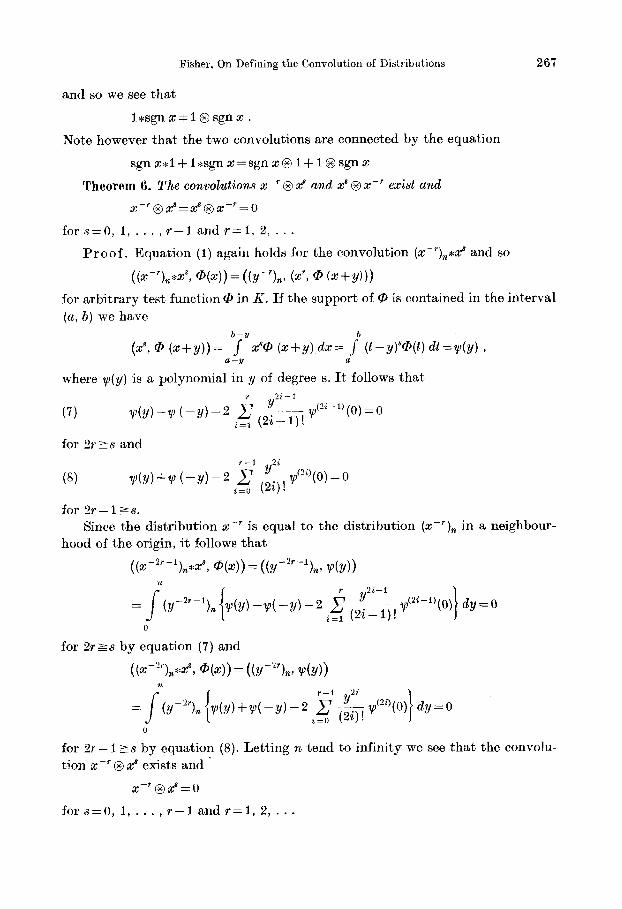
and so we see that

l s s g n x + l @ s g n x .

Note however that the two convolutions are connected by the equation

sgn xhl + lssgn x=sgn x @ 1 + 1 @ sgn x Theorem 6. The convolutions xPr 0 x8 and x8 0 xPr exist and

x -r @ x* =xs 0 x-+- = 0

for s=O, 1, . . . , r -1 and r = l , 2, . . . P r o o f . Equation (1) again holds for the convolution (x-'),xx8 and SO

((X-7),*xR, @(x))= ((y-p),, (ZS, 0 (z+y)))

for arbitrary test function Q, in K . If the support of @ is contained in the interval (a, b ) we have

b - u b

(x8, @ (x+y))= J xsO (x+y) dx= I' (t-y)%?(t) d t=y (y ) , a --Y a

where y(y) is a polynomial in 9 of degree s. It follows that

for 2r z,s and

for 2r - 1 zs.

hood of the origin, it follows that Since the distribution x - ~ is equal to the distribution (x - ' )~ in a neighbour-

((x-2r-l),*28, @(x)) = ((y--),, y ( y ) )

0

for 2 r z s by equation (7) and

for 2r - i --IS by equation (8). Letting rb tend to infinity we see that the convolu- tion x-'@x8 exists and .

x-' ox" = 0

for s=0, 1 , . . . , r - 1 and r = l , 2, . . .

268 Fisher, On Defining the Convolutiun of Distributions

Next we have

((58)n*5-r, @(5))= (y-', (W),, di (z+y)))

for arbitrary test function @ in K . If the support of di is contained in the interval (a, b ) we have

b-U I #

( ( x 8 ) , , @ (s+Y))= J ( 2 ) n Q (%+Y) dx= J ( ( f - g ) 8 ) n @ ( t ) d t = ~ g t ( y ) *

(I-U a

1 1

'I 2 This time y,(y) is a polynomial only if b - ~ n s y s a + - n and y,(y) = 0 if

y z b + n or y s a - n . Thus for all n=-4 lal, 4 Ibl we have y,(y) satisfies equation (7) in the interval ( - n / 4 , % / 4 ) for 2 r z s and satisfies equation (8) in the interval ( - n I 4 , n i 4 ) for 2r - 1 z s . Further y*(y)=O for 19, z5nI4 and so for 2 r s s

( ( 5 8 ) , t * 5 - 2 r - 1 , @(5))= (y-?? y&))

8114

where

as ?E. tends to infinity and

If 2r=-.s then I1 obviously converges to zero as n tends to infinity and if 2 r = ~ 514 b

I , = j- v-2r-1 f (( (t/n - W)'L')% - ( ( t / n + v)"),} @(t) dt dv , I / ,* fl

where

(Wn - w ) " ) , ~ - ( ( t /n+w) ' r ) .

= ( t i n - W ) ' ' ~ Z (t/n - w) - ( t / n + ~ ) ' ~ t ( t / n + r )

converges uniformly to zero with 1/4 sv 5 514 and a st s b . It follows that

for 2r 2 s and all test functions 0 in K .

Fisher, On Defining the Convolution of Distributions 269

r--i YZi y-2r c __ y p ( 0 ) dy-0 s (2i)! J2= - 2

514 b j" vbZr

114 a {(( t /n-v)8)n+ ((t/n+v)'),) @(t) dt dv . - -2r+ 1 -

If 2r - 1 =-s then J, obviously converges to zero as n tends to infinity and if 2r - 1 = s 514 b

J,=

((t /n-v)2'-i)n+ ( t / n + ~ ) ~ ' - ~ ) ~

v-2' j"{(( t /n-v)2r-1)n+(( t /n+v)2r-~) , ) @(t) dt dv , 114 a

where

converges uniformly to zero with 1/4 sv 5 5/4 and a st s b . It follows that

for 2r - 1 zs and all test functions @ in K . We have therefore proved that the convolution x* 0 x - ~ exists and

x a @ z - r = o

for s = 0, 1, 2, . . . , r - 1 and r = 1, 2, . . . This completes the proof of the theorem. Comparing the results of this theorem with equation (4) we Bee that definitions

3 and 4 are in agreement for the convolutions of the distributions zE and x - ~ .

References

[l] B. FISHER, The convolution x-'*xs, Glasgow Math. J., 17, 53-6, (1976). [2] -, A result on the convolution of distributions, Proc. Edinburgh Math. SOC., 19, 393-5, (1975). [3] I. M. GELFAND and G. E. S m o v , Generalized functions, Vol. I, (1964). [4] D. S. JONES, The convolution of generalized functions, Quart. J. Math. Oxford Ser. (2), 24,

145-63, (1973).

Department of Mathematics The University Leicester LEI 7RH Great Britain