On Crossing Numbers of Geometric Proximity Graphs

Bernardo M. Abrego∗ Ruy Fabila-Monroy† Silvia Fernandez-Merchant∗

David Flores-Penaloza‡ Ferran Hurtado§ Vera Sacristan§ Maria Saumell§

Abstract

Let P be a set of n points in the plane. A geometric proximity graph on P is a graph wheretwo points are connected by a straight-line segment if they satisfy some prescribed proximityrule. We consider four classes of higher order proximity graphs, namely, the k-nearest neighborgraph, the k-relative neighborhood graph, the k-Gabriel graph and the k-Delaunay graph. Fork = 0 (k = 1 in the case of the k-nearest neighbor graph) these graphs are plane, but for highervalues of k in general they contain crossings. In this paper we provide lower and upper boundson their minimum and maximum number of crossings. We give general bounds and we alsostudy particular cases that are especially interesting from the viewpoint of applications. Thesecases include the 1-Delaunay graph and the k-nearest neighbor graph for small values of k.

Keywords Proximity graphs; geometric graphs; crossing number.

1 Introduction and basic notation

A geometric graph on a point set P is a pair G = (P,E) in which the vertex set P is assumed to bein general position, i.e., no three points are collinear, and the set E of edges consists of straight-linesegments with endpoints in P . Notice that the focus is more on the drawing rather than on theunderlying graph, as carefully pointed out by Brass, Moser and Pach in their survey book ([6], page373).

A proximity graph is a graph G = (V,E) in which the nodes represent geometric objects in agiven set, typically points, and two nodes are adjacent when the corresponding objects are consid-ered to be neighbors according to some specific proximity criterion. A geometric proximity graphis a geometric graph in which the adjacency is decided by some neighborhood rule; they are alsosometimes called proximity drawings [18]. Examples of these graphs are the k-nearest neighborgraph, k-NNG(P ), in which every point is joined with a directed segment to its k closest neighbors,and the k-Delaunay graph, k-DG(P ), in which pi and pj are connected with a segment if there issome circle through pi and pj that contains at most k points from P in its interior. Other similardefinitions are given later in this paper.

Proximity graphs have been widely used in applications in which extracting shape or structurefrom a point set is a required tool or even the main goal, as is the case of computer vision, pattern

∗Department of Mathematics, California State University, Northridge, CA,{bernardo.abrego,silvia.fernandez}@csun.edu.

†Departamento de Matematicas, CINVESTAV, Mexico DF, Mexico, ruyfabila@math.cinvestav.edu.mx.‡Departamento de Matematicas, Facultad de Ciencias, Universidad Nacional Autonoma de Mexico,

dflorespenaloza@gmail.com.§Departament de Matematica Aplicada II, Universitat Politecnica de Catalunya, Barcelona, Spain,

{ferran.hurtado,vera.sacristan,maria.saumell}@upc.edu. Partially supported by projects MTM2009-07242 andGen. Cat. DGR 2009SGR1040.

1

recognition, visual perception, geographic information systems, instance-based learning, and datamining [13, 19, 26]. In the area of graph drawing [5, 12, 14] the main goal is to realize —or todraw— a given combinatorial graph as a geometric proximity graph, which leads to problems oncharacterizing the graphs that admit such a representation and designing efficient algorithms toconstruct the drawing whenever possible (see the survey [18] in this respect).

Usually graphs are drawn in the plane with points as nodes and Jordan arcs as edges. Whentwo edges share an interior point, we say that there is a crossing. Both as a natural aestheticmeasure for graph drawing and as a fundamental issue in the mathematical context, the number ofcrossings is a parameter that has been attracting extensive study. Given a graph G, the crossingnumber of G, denoted by cr(G), is the minimum number of edge crossings in any drawing of G; ifthis number is 0, we say that the graph is planar. The rectilinear crossing number of G, denoted bycr(G), is the smallest number of crossings in any drawing of G in which the edges are representedby straight-line segments.

Computing the crossing number of a graph is an NP-hard problem [9], and both the generic andrectilinear crossing numbers of very fundamental graphs, such as the complete graph Kn and thecomplete bipartite graph Km,n are still unknown [29, 11]. These problems have been attracting agreat amount of attention and recently a continuous chain of improvements has led progressivelyto narrow the gap between the lower and upper bounds [15, 3, 2]. There are also several resultson the numbers of crossings that are sensitive to the size of the graph —particulary the crossinglemma [4, 17, 6]—, or to the exclusion of some configurations [6, 20, 22, 28, 8].

In this paper we study the crossing numbers of several higher order geometric proximity graphsrelated to Delaunay graphs. If P is a set of points in the plane, each of the proximity graphs weconsider is a geometric graph on P that has some number of crossings that will be denoted by £ ( ),and we investigate how this number varies when all possible point sets P in general position, with|P | = n, are considered. The generic conclusion that may be derived from our research is that thisfamily of graphs has a relatively small number of crossings.

The fact that this specific issue has not been investigated previously is somehow surprising. Asan explanation, one may first consider that 0-order proximity graphs, which have attracted most ofthe research and are better understood, are planar. On the other hand, regarding the applications inshape analysis, the data are what they are, and the user would not have the possibility of movingthe points around to decrease the number of crossings. It is worth mentioning here that, whilehigher order proximity graphs were introduced and studied about twenty years ago [24, 25], therehas been a renewal of interest on them, especially for low orders, as they offer a flexibility whichis desirable in several applications. For example, the Delaunay triangulation (DT) is unique, whileone can extract a large number of different triangulations from the 1-Delaunay graph, all of them“close” to DT, which may be preferable under some criterion (see for example the papers [16, 1]and the numerous references there).

From the viewpoint of proximity drawings, it is desirable to have a small number of crossings,and hence we study its minimum value. On the other hand, we also consider the shape analysissituation in which choosing the points is not possible, which leads to study how large the numberof crossings can be, i.e., its maximum value.

For example, consider the k-nearest neighbor graph of point sets P with |P | = n. We introduceand study the rectilinear crossing number and the worst crossing number defined respectively as

cr(k-NNG(n)) = min|P |=n

£ (k-NNG(P )),

wcr(k-NNG(n)) = max|P |=n

£ (k-NNG(P )).

We define analogous parameters for the k-relative neighborhood graph, k-RNG(P ), in which

2

pi, pj are adjacent if the open intersection of the circles centered at pi and pj with radius |pipj |contains at most k points from P ; the k-Gabriel graph, k-GG(P ), in which pi and pj are adjacentif the closed circle with diameter pipj contains at most k points from P different from pi, pj ; andthe k-Delaunay graph, k-DG(P ). It is well known that

(k + 1)-NNG(P) ⊆ k-RNG(P ) ⊆ k-GG(P ) ⊆ k-DG(P ). (1)

Notice that, when the rectilinear crossing number of a combinatorial graph is considered, wedraw the same graph on top of different points sets, while here we study a specific kind of proximitygraph on top of different point sets, but the underlying combinatorial graphs may be different formany of these sets. Another somehow subtle issue that deserves a specific comment is the fact thatthe combinatorial graph obtained from a proximity drawing may have a smaller crossing numberthan the rectilinear crossing number of its proximity drawing. This is clearer with an example: Weprove in this paper that cr(1-DG(n)) = n − 4; this means that 1-DG(P ) contains at least n − 4crossings for any set P of n points, and that for some point set Q this number is achieved. Thegraph on Figure 1 (left) is the 1-Delaunay graph of its vertex set (the six shown points) and has 2crossings; however, the combinatorial graph can be drawn on top of a different set and have onlyone crossing (Figure 1, right). Obviously the latter is not the 1-Delaunay graph of its vertex set.

b b′

d f ′c

f

d′ c′

e e′

a a′

Figure 1: The graph on the left is a 1-Delaunay graph; black edges belong to 0-DG. The graph onthe right is isomorphic.

A substantial part of our research focus on the 1-Delaunay graph and on the graphs k-NNG(P )with small k, widely used in classification scenarios, as these are the most interesting situationsfrom the viewpoint of applications [1, 7, 10, 16]. We present these results in Subsections 2.1 and 2.2.In Subsection 2.3 we look at the number of crossings for large values of k. Throughout the paperwe assume that point sets P are in general position in an extended sense meaning: no three pointsare collinear, no four points are concyclic and, for each p ∈ P, the set of its k nearest points in Pis well-defined, i.e., has cardinality k, for any k ≥ 1.

Throughout the paper we denote by V (G) (respectively, E(G)) the set of vertices (respectively,edges) of a given graph G, and by v(G) (respectively, e(G)) the cardinality of this set. If v is avertex in V (G), we denote by dG(v) the degree of v in G. We consider a generic set P of n pointsin general position, and we denote by h the size of the convex hull of P .

2 Results

Given the number of results in the paper and the length of some proofs, in this section we onlystate our bounds deferring the proofs to the subsequent section.

3

2.1 1-Delaunay graphs

In this subsection we carry out a detailed analysis of the number of crossings in a 1-Delaunay graph.We study the general case and also the particular case where all points are in convex position. Ourcontributions are presented in Table 1. Note that we establish the exact value of the rectilinearcrossing number of the 1-Delaunay graph for both the general case and the convex case.

general case convex case

cr n− 4 6n− 3bn2 c − 19

wcr n2 + Θ(n) ≤wcr≤ 4n2 + Θ(n) n2

2 + Θ(n) ≤wcr≤ 7n2

8 + Θ(n)

Table 1: 1-Delaunay graphs.

As shown in [1], the number of elements in E(1-DG(P ))−E(0-DG(P )) is linear. Since 0-DG(P )is maximal planar, this immediately yields that every 1-Delaunay graph contains a linear numberof crossings. More accurate observations lead to the following bound:

Theorem 2.1.1. For every point set P, £ (1-DG(P )) ≥ n− 4.

Proposition 2.1.2. There exists a point set Q such that £ (1-DG(Q)) = n− 4.

If P is in convex position, the bounds can be strengthened:

Theorem 2.1.3. For every set P in convex position, £ (1-DG(P )) ≥ 6n− 3bn2 c − 19.

Proposition 2.1.4. There exists a point set Q in convex position such that £ (1-DG(Q)) = 6n −3bn

2 c − 19.

In principle, every pair of edges in E(1-DG(P )) − E(0-DG(P )) might cross, so the number ofcrossings in 1-DG(P ) could be quadratic. In the following lines we provide quadratic upper boundson the number of crossings of 1-DG(P ), and show that in some cases this parameter is indeedquadratic.

Theorem 2.1.5. For every set of points P, £ (1-DG(P )) ≤ 4n2 + Θ(n).

Proposition 2.1.6. There exists a point set Q such that £ (1-DG(Q)) = n2 + Θ(n).

For the convex case we prove tighter bounds:

Theorem 2.1.7. For every set of points P in convex position, £ (1-DG(P )) ≤ 7n2/8 + Θ(n).

Proposition 2.1.8. There exists a set of points Q in convex position such that £ (1-DG(Q)) =n2/2 + Θ(n).

2.2 k-nearest neighbor graphs for small values of k

We provide bounds on the rectilinear crossing number of the k-nearest neighbor graph k-NNG fork ≤ 10. Due to the inclusion relations satisfied by the graphs we investigate, the lower bounds alsohold for the rectilinear crossing number of the other proximity graphs if we shift the value of k oneunit down (see (1)).

Our results are summarized in Table 2. It is interesting noticing that, even though the lowerbounds do not rely on specific properties of k-NNG but on generic results, for many values of k weare able to construct point sets attaining these bounds.

4

Theorem 2.2.1. The rectilinear crossing number of k-NNG, when k ∈ {1, 2, . . . , 10}, satisfies theequalities and inequalities shown in Table 2.

k cr(k-NNG(n))

1 0

2 0

3 0

4 0, for n ≥ 14

5 0, for n ≥ 44

6 ≤ 58, for n ≥ 39

7 n/2 + Θ(1)

8 n + Θ(1)

9 13n/6 + 50/3 ≤ cr≤ 31n/13 + Θ(1)

10 10n/3 + 50/3 ≤ cr≤ 4n + Θ(1)

Table 2: cr(k-NNG(n)) for the first values of k.

As for the worst crossing number, we will give bounds for all k in Subsection 2.3, and we canimprove on these only minimally for small k. Thus we omit those details.

2.3 General bounds

In this subsection we are interested in the number of crossings in the graphs under study when thevalue of k is large. We have derived bounds for both the rectilinear crossing number and the worstcrossing number of all graphs (see Table 3). Observe that in all cases we can specify the exact orderof magnitude of these parameters up to multiplicative constants.

k-NNG(n) k-RNG(n) k-GG(n) k-DG(n)

cr ≥ 12831827k3n 128

31827k3n 12831827k3n 1024

31827k3n

cr≤ 19π2 k3n π

9(2π/3−√3/2)3k3n 64

9π2 k3n 649π2 k3n

wcr≥ 13k3n 1

3k3n 14k2n2 1

2k2n2

wcr≤ k3n 9k3n 3k2n2 3k2n2

Table 3: Dominant terms of the general bounds. Some of the bounds only hold for “intermediate”values of k. We refer to the precise statements in the rest of the subsection.

2.3.1 Rectilinear crossing number

Our lower bounds for the rectilinear crossing numbers follow from an improved version of thecrossing lemma given in [21].

Theorem 2.3.1. If k ≥ 13, then

5

i) cr(k-NNG(n)) ≥ 12831827k3n,

ii) cr(k-RNG(n)) ≥ 12831827k3n,

iii) cr(k-GG(n)) ≥ 12831827k3n.

If 6 ≤ k < n2 − 1, then

iv) cr(k-DG(n)) ≥ 102431827k3n.

As already observed in [1], if k ≥ n2 − 1, then k-DG(P ) is the complete graph.

For the upper bounds we use a suitable construction proposed in [23]. This construction is thecurrent asymptotically best example of a graph with fixed number of edges and minimum numberof crossings. In the next proposition we show that it can be seen as a proximity graph.

Proposition 2.3.2. If ω(1) ≤ k ≤ o(n), there exists a point set Q such that

i) £ (k-NNG(Q)) ≤ 19π2 k3n(1 + o(1)),

ii) £ (k-RNG(Q)) ≤ π9(2π/3−√3/2)3

k3n(1 + o(1)),

iii) £ (k-GG(Q)) ≤ 649π2 k3n(1 + o(1)),

iv) £ (k-DG(Q)) ≤ 649π2 k3n(1 + o(1)).

2.3.2 Worst crossing number

Any upper bound on the number of edges of some higher order proximity graph can be used toproduce an upper bound on its worst crossing number. For k-Delaunay graphs, it has been provedthat the number of edges is at most 3(k + 1)n− 3(k + 1)(k + 2) [1]. In the worst scenario, all pairsof edges might cross, so the number of crossings is no more than 9

2k2n2 + o(k2n2). In the followingtheorem we improve this bound:

Theorem 2.3.3. For every point set P, if k < n/2 − 1, then £ (k-GG(P )) ≤ £ (k-DG(P )) ≤(3k2 + 6k + 3)n2 + (−6k3 − 21k2 − 51

2 k − 212 )n + (3k4 + 15k3 + 57

2 k2 + 512 k + 9).

The preceding bounds are tight up to a multiplicative constant:

Proposition 2.3.4. If k = o(n), there exists a point set Q such that £ (k-GG(Q)) = k2n2/4 +o(k2n2).

Proposition 2.3.5. If k = o(n), there exists a point set Q such that £ (k-DG(Q)) = k2n2/2 +o(k2n2).

For k-relative neighborhood graphs, it can be shown that the number of edges is bounded fromabove by 3kn + 3n (see Appendix), which yields an upper bound of 9k2n2 + o(k2n2) for the worstcrossing number. We have proved that the order of magnitude of this parameter is lower providedthat k = o(n):

Theorem 2.3.6. For every point set P, £ (k-RNG(P )) ≤ (9k2 + 18k + 9)kn.

Finally, the number of edges of k-NNG is no greater than kn. In this case Theorem 2.3.7 andProposition 2.3.8 show that the worst crossing number is also cubic in k and linear in n:

Theorem 2.3.7. For every point set P, £ (k-NNG(P )) ≤ (2k2 − 3k + 1)kn/2.

Proposition 2.3.8. If k = o(n), there exists a point set Q such that £ (k-RNG(Q)) ≥ £ (k-NNG(Q)) =k3n/3 + o(k3n).

6

3 Proofs

3.1 Proofs of the results in Subsection 2.1

Let us introduce some notation. We partition the edges of the 1-Delaunay graph into two groups:we say that an edge is blue if it also appears in 0-DG(P ) and we say that it is red otherwise. Weset eb = e (0-DG(P )) and er = e (1-DG(P )) − e (0-DG(P )). Note that a red edge pipj correspondsto an element in E(0-DG(P r {pl})) for some pl ∈ P. We say that pipj is generated by pl. Observethat the fact that pipj is generated by pl is equivalent to the existence of a disk through pi andpj containing pl and no other point in P , which implies that pipl and pjpl belong to E(0-DG(P )).Thus pipj is generated by at most two points. (See [1].)

In the figures of this subsection the blue edges will be represented in black and the red edgeswill be represented in gray.

3.1.1 Proof of Theorem 2.1.1

Since the graph 0-DG(P ) is maximal planar, each red edge induces at least one crossing in 1-DG(P ).We prove that the number of red edges in 1-DG(P ) is at least n − 4 (see Theorem 3.1.5). Part ofour proof follows the lines of previous techniques used in [1].

Let us introduce some notation. Let H and I be the convex and interior points of P. Forconvenience, sets are denoted with a capital letter and their cardinalities with the correspondinglower case letter (thus h and i denote the cardinality of H and I respectively).

For a point p ∈ P , let dG(p) denote the degree of p in G, where G = 0-DG(P ), and let d∗(p) bethe value 2 plus the number of points of I that are in the convex hull of P r {p}.

Our proof requires several remarks, already stated in [1]:

Lemma 3.1.1. The set of red edges generated by exactly two points induces a perfect matching onthe triangles of 0-DG(P ). Moreover, two so matched triangles are adjacent triangles of 0-DG(P ) inconvex position.

Lemma 3.1.2. The number of red edges generated by an element p ∈ P is:

• dG(p)− d∗(p), if p ∈ H;

• dG(p)− 3, if p ∈ I.

Lemma 3.1.3. If pl ∈ I is in the convex hull of both P r {pi} and P r {pj}, for some pair ofpoints pi, pj ∈ H, then pi and pj are consecutive vertices in the convex hull of P . Furthermore, thetriangle 4pipjpl is empty, and the line through pi and pl separates 4pipjpl from the rest of P , asdoes the line through pj and pl.

Lemma 3.1.4. Each element of I can contribute to d∗(pi) and d∗(pj) for at most two pointspi, pj ∈ H, provided that n ≥ 5.

By Lemma 3.1.4, we may partition I into I0 ∪ I1 ∪ I2, where Ij is the set of elements of I thatcontribute to d∗ for exactly j points.

Notice that, if pl ∈ I2 contributes to d∗ for pi and pj , then, by Lemma 3.1.3, the points pi, pj ,and pl together with any other point of P are not in convex position. Hence 4pipjpl is a triangleof 0-DG(P ) that does not participate in the matching given by Lemma 3.1.1. Such a triangle iscalled special triangle.

7

We wish to bound the number of red edges in 1-DG(P ). By Lemma 3.1.2,

er =∑

p∈H

(dG(p)− d∗(p)) +∑

p∈I

(dG(p)− 3)− ξ =

= 4n− 6− (i +∑

p∈H

d∗(p))− ξ, (2)

where is ξ the number of times a red edge is overcounted in the summation (which happenswhen two points induce the same edge). Since the set of red edges generated by the removal of twopoints induces a matching in the triangles of 0-DG(P ), we may now introduce a new equation:

ξ =4− i2 −m

2, (3)

where 4 is the number of triangles in 0-DG(P ) (thus 4 = h + 2i− 2), and m is the number ofnon-special triangles in 0-DG(P ) not matched by a red edge generated by two points.

Substituting (3) in (2) and using that∑

p∈H d∗(p) = 2h + i1 + 2i2, we obtain that

er = n− 5 + i0 +12

(h− i2 + m) .

Since i0 ≥ 0, h− i2 ≥ 0, and m ≥ 0, we have that er ≥ n− 5, and er = n− 5 if and only if:

i0 = 0, h = i2, and m = 0. (4)

We make some observations about the structure of P in the case where (4) is satisfied andintroduce some useful notation.

Note that any point that contributes to d∗ for some other point of H is in the second convexlayer of P . Therefore if we assume that i0 = 0, then P has exactly two convex layers, and thesecond one is given by the set I = I2 ∪ I1. We say that each point pl ∈ I2 is associated to twopoints of H: those points for whom q contributes to d∗. Similarly, each point pl ∈ I1 is associatedto the point pi ∈ H for which pl contributes to d∗(pi).

With these last observations we are ready to prove a lower bound on the number of red edges.

Theorem 3.1.5. The graph 1-DG(P ) contains at least n− 4 red edges.

Proof. Suppose by means of a contradiction that er = n− 5 and thus (4) holds.

We distinguish two cases.

First we assume that every edge of the convex hull of I is an edge of 0-DG(P ). In this caseevery triangle having exactly one point of H as a vertex is entirely contained between the firstand second convex layers of P ; see Figure 2 (left). No two of these triangles are matched, becausethe four vertices of two such adjacent triangles are not in convex position. As m = 0 and thespecial triangles cannot be matched, we infer that every triangle having exactly one point of H asa vertex is matched with one triangle contained in the second convex layer of P . However, thereare i triangles of the first type and i − 2 triangles of the second type. Thus i0 = 0, h = i2, andm = 0 cannot simultaneously hold in this case.

8

pi

pm

pj

pl

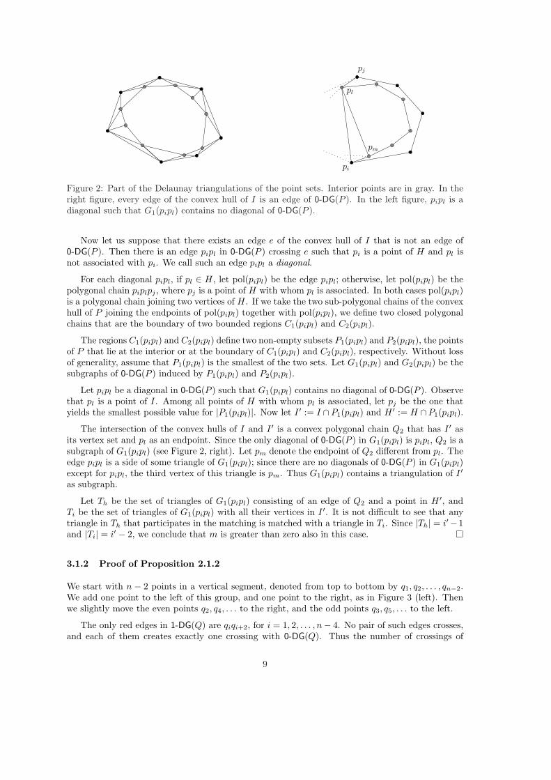
Figure 2: Part of the Delaunay triangulations of the point sets. Interior points are in gray. In theright figure, every edge of the convex hull of I is an edge of 0-DG(P ). In the left figure, pipl is adiagonal such that G1(pipl) contains no diagonal of 0-DG(P ).

Now let us suppose that there exists an edge e of the convex hull of I that is not an edge of0-DG(P ). Then there is an edge pipl in 0-DG(P ) crossing e such that pi is a point of H and pl isnot associated with pi. We call such an edge pipl a diagonal.

For each diagonal pipl, if pl ∈ H, let pol(pipl) be the edge pipl; otherwise, let pol(pipl) be thepolygonal chain piplpj , where pj is a point of H with whom pl is associated. In both cases pol(pipl)is a polygonal chain joining two vertices of H. If we take the two sub-polygonal chains of the convexhull of P joining the endpoints of pol(pipl) together with pol(pipl), we define two closed polygonalchains that are the boundary of two bounded regions C1(pipl) and C2(pipl).

The regions C1(pipl) and C2(pipl) define two non-empty subsets P1(pipl) and P2(pipl), the pointsof P that lie at the interior or at the boundary of C1(pipl) and C2(pipl), respectively. Without lossof generality, assume that P1(pipl) is the smallest of the two sets. Let G1(pipl) and G2(pipl) be thesubgraphs of 0-DG(P ) induced by P1(pipl) and P2(pipl).

Let pipl be a diagonal in 0-DG(P ) such that G1(pipl) contains no diagonal of 0-DG(P ). Observethat pl is a point of I. Among all points of H with whom pl is associated, let pj be the one thatyields the smallest possible value for |P1(pipl)|. Now let I ′ := I ∩ P1(pipl) and H ′ := H ∩ P1(pipl).

The intersection of the convex hulls of I and I ′ is a convex polygonal chain Q2 that has I ′ asits vertex set and pl as an endpoint. Since the only diagonal of 0-DG(P ) in G1(pipl) is pipl, Q2 is asubgraph of G1(pipl) (see Figure 2, right). Let pm denote the endpoint of Q2 different from pl. Theedge pipl is a side of some triangle of G1(pipl); since there are no diagonals of 0-DG(P ) in G1(pipl)except for pipl, the third vertex of this triangle is pm. Thus G1(pipl) contains a triangulation of I ′

as subgraph.

Let Th be the set of triangles of G1(pipl) consisting of an edge of Q2 and a point in H ′, andTi be the set of triangles of G1(pipl) with all their vertices in I ′. It is not difficult to see that anytriangle in Th that participates in the matching is matched with a triangle in Ti. Since |Th| = i′−1and |Ti| = i′ − 2, we conclude that m is greater than zero also in this case.

3.1.2 Proof of Proposition 2.1.2

We start with n − 2 points in a vertical segment, denoted from top to bottom by q1, q2, . . . , qn−2.We add one point to the left of this group, and one point to the right, as in Figure 3 (left). Thenwe slightly move the even points q2, q4, . . . to the right, and the odd points q3, q5, . . . to the left.

The only red edges in 1-DG(Q) are qiqi+2, for i = 1, 2, . . . , n− 4. No pair of such edges crosses,and each of them creates exactly one crossing with 0-DG(Q). Thus the number of crossings of

9

1-DG(Q) is n− 4.

3.1.3 Proof of Theorem 2.1.3

Let p1, . . . , pn denote the points in P in clockwise order. Note that all edges of type pipi+2 are in1-DG(P ), and that the total number of crossings between two edges of this family is n. Let G′ bethe graph obtained from 1-DG(P ) by removing these edges and the ones in the convex hull of P.Since er ≥ 2n − bn

2 c − 5 (see [1]), G′ contains at least 2n − bn2 c − 8 edges. Each of them induces

two crossings with the edges that have been removed.

Let G′p be a maximal planar subgraph of G′. It is easy to see that G′p contains at most n − 5edges. Thus there are at least n−bn

2 c− 3 edges in G′ but not in G′p, each of which induces at leastone crossing with an edge of G′p.

Adding everything up, the graph 1-DG(P ) has no less than 6n− 3bn2 c − 19 crossings.

3.1.4 Proof of Proposition 2.1.4

Consider two horizontal lines such that each point in one line has a counterpart in the other linewith the same abscissa. Add one point to the left of both lines such that its ordinate is the averageof the ordinates of the lines. If the positions of the points are carefully chosen, it is possible toperturb them so that the point set is in convex position and 1-DG(Q) contains only the edges drawnin Figure 3 (middle). Easy calculations show that, in this case, the number of crossings of the graphis 6n− 3bn

2 c − 19.

Figure 3: Left: point set whose 1-Delaunay graph has n− 4 crossings. Middle: point set in convexposition whose 1-Delaunay graph has 6n− 3bn

2 c− 19 crossings. Right: point set in convex positionwhose 1-Delaunay graph has n2/2 + Θ(n) crossings.

3.1.5 Proof of Theorem 2.1.5

Theorem 2.3.3 says that at most 12n2 − 63n + 81 crossings are present in 1-DG(P ). In this proofwe improve the dominant term of this bound to 4n2.

A crossing in 1-DG(P ) is caused either by a red edge and a blue one or by a pair of red edges. Wedenote the cardinal number of the first and second sets of crossings by r⊗ b and r⊗ r, respectively.We derive upper bounds for r ⊗ b and r ⊗ r.

The bound for r ⊗ b is given in Lemma 3.1.9 and requires several technical lemmas and obser-vations:Observation 3.1.6. Let pipj , plpm be two crossing edges. Either every circle through pi, pj containspl or pm, or every circle through pl, pm contains pi or pj .

10

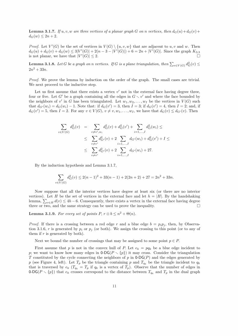
Lemma 3.1.7. If u, v, w are three vertices of a planar graph G on n vertices, then dG(u)+dG(v)+dG(w) ≤ 2n + 2.

Proof. Let V ′(G) be the set of vertices in V (G) \ {u, v, w} that are adjacent to u, v and w. ThendG(u) + dG(v) + dG(w) ≤ 3|V ′(G)|+ 2(n− 3− |V ′(G)|) + 6 = 2n + |V ′(G)|. Since the graph K3,3

is not planar, we have that |V ′(G)| ≤ 2.

Lemma 3.1.8. Let G be a graph on n vertices. If G is a plane triangulation, then∑

v∈V (G) d2G(v) ≤

2n2 + 33n.

Proof. We prove the lemma by induction on the order of the graph. The small cases are trivial.We next proceed to the inductive step.

Let us first assume that there exists a vertex v′ not in the external face having degree three,four or five. Let G′ be a graph containing all the edges in G r v′ and where the face bounded bythe neighbors of v′ in G has been triangulated. Let w1, w2, . . . , wI be the vertices in V (G) suchthat dG′(wi) = dG(wi)− 1. Note that: if dG(v′) = 3, then I = 3; if dG(v′) = 4, then I = 2; and, ifdG(v′) = 5, then I = 2. For any v ∈ V (G), v 6= v, w1, . . . , wI , we have that dG(v) ≤ dG′(v). Then

∑

v∈V (G)

d2G(v) =

∑

v 6=v′,wi

d2G(v) + d2

G(v′) +∑

i=1,...,I

d2G(wi) ≤

≤∑

v 6=v′d2

G′(v) + 2∑

i=1,...,I

dG′(wi) + d2G(v′) + I ≤

≤∑

v 6=v′d2

G′(v) + 2∑

i=1,...,I

dG′(wi) + 27.

By the induction hypothesis and Lemma 3.1.7,

∑

v∈V (G)

d2G(v) ≤ 2(n− 1)2 + 33(n− 1) + 2(2n + 2) + 27 = 2n2 + 33n.

Now suppose that all the interior vertices have degree at least six (or there are no interiorvertices). Let H be the set of vertices in the external face and let h = |H|. By the handshakinglemma,

∑v∈H d(v) ≤ 4h− 6. Consequently, there exists a vertex in the external face having degree

three or two, and the same strategy can be used to prove the inequality.

Lemma 3.1.9. For every set of points P, r ⊗ b ≤ n2 + Θ(n).

Proof. If there is a crossing between a red edge r and a blue edge b = pipj , then, by Observa-tion 3.1.6, r is generated by pi or pj (or both). We assign the crossing to this point (or to any ofthem if r is generated by both).

Next we bound the number of crossings that may be assigned to some point p ∈ P.

First assume that p is not in the convex hull of P. Let ek = pqk be a blue edge incident top; we want to know how many edges in 0-DG(P r {p}) it may cross. Consider the triangulationT constituted by the cycle connecting the neighbors of p in 0-DG(P ) and the edges generated byp (see Figure 4, left). Let Tp be the triangle containing p and Tqk

be the triangle incident to qk

that is traversed by ek (Tqk= Tp if qk is a vertex of Tp). Observe that the number of edges in

0-DG(P r {p}) that ek crosses correspond to the distance between Tqkand Tp in the dual graph

11

of T . Observe also that, if qk and ql are two different vertices that are adjacent to p in 0-DG(P )and are not vertices of Tp, we have that Tqk

6= Tql. Then it is easy to see that the configuration

of the dual graph maximizing the sum of distances between Tqkand Tp, for all qk neighbor of p in

0-DG(P ) (and not vertex of Tp), is a tree rooted at Tp. Consequently, at most∑dG(p)−3

ν=1 ν crossings(where G = 0-DG(P )) are assigned to p.

Next suppose that p is a vertex of the convex hull of P . Let q1, q2, . . . , qdG(p) be the neighbors ofp in 0-DG(P ) in radial order around p (G = 0-DG(P )). Let qτ be the first point that belongs to theconvex hull of P r {p} but does not belong to the convex hull of P (if there is not such qτ , we setqτ = qdG(p)). Let us look at the triangulation of the polygon pq1q2 . . . qτp given by the red edges.In order to determine the number of edges in 0-DG(P r{p}) that an edge pqk (k ∈ {2, 3, . . . , τ −1})crosses we can use the same argument as before, except that in this case Tp is defined as the trianglehaving p as a vertex. Next we can look at the next point that belongs to the convex hull of P r{p}but does not belong to the convex hull of P (let us denote it by qι) and apply the same argumentto the edges of the polygon pqτqτ+1 . . . qιp. We proceed in this way until we reach qdG(p). Then itis not difficult to see that the number of crossing that may be assigned to p is less than or equal to∑dG(p)−2

ν=1 ν.

Now the result follows from Lemma 3.1.8.

p

p

qk

q1

q2

qd(p)

qτ

Figure 4: Crossings assigned to p. In the right figure, p is an interior point of P ; in the leftfigure, it belongs to the convex hull of P . The dashed edges correspond to the dual graphs of thetriangulations given by the red edges.

Next we give an upper bound for r ⊗ r, which, combined with the bound just seen, completesthe proof of Theorem 2.1.5.

Lemma 3.1.10. For every set of points P, r ⊗ r ≤ 3n2 + Θ(n).

Proof. Let the red crossing graph be the graph whose vertices are the red edges of 1-DG(P ) andwhere two vertices are adjacent if their corresponding edges cross. First we will prove that er ≤3n− h− 6, that is, that the red crossing graph has no more than 3n− h− 6 vertices. Afterwardswe will see that every red crossing graph has no 4-clique. Then we can apply Turan’s theorem [27],which states that any Kr+1-free graph on m vertices has at most (1− 1

r )m2

2 edges. This yields theresult.

First we bound the number of vertices of the red crossing graph.

Let H be the set of points in the convex hull of P , I be the set of interior points of P , andIj (j ∈ {0, 1, 2}) be the set of interior points of P appearing in the convex hull of P r {p} for jdistinct points p ∈ H. We denote the cardinal number of these sets by the corresponding lower caseletter. For p ∈ H, let d∗(p) be the value 2 plus the number of points of the convex hull of P r {p}

12

which are not vertices of the convex hull of P . Finally, let ξ be the number of red edges that aregenerated by two distinct points of P . We have already seen that

er = 4n− 6− (i +∑

p∈H

d∗(p))− ξ.

Using that∑

p∈H d∗(p) = 2h + i1 + 2i2, we obtain that

er = 2n− 6 + i0 − i2 − ξ.

Substituting i0 ≤ n− h, i2 ≥ 0, and ξ ≥ 0, we can conclude

er ≤ 3n− h− 6.

Next we prove that the red crossing graph is K4-free.

By Observation 3.1.6, if two red edges pipj , plpm cross, either every circle through pi, pj containspl or pm, or viceversa. If every circle through pi, pj contains pl or pm, we say that plpm constrainspipj .

Let pipj , plpm, and pspt be three pairwise crossing red edges. Since all the endpoints of theseedges are distinct, every edge can only be constrained by one of the other two. Thus, without lossof generality, we can assume that plpm constrains pipj , pspt constrains plpm, and pipj constrainspspt. Now suppose that there exists a red edge pupv that crosses pipj , plpm, and pspt. Then pupv

must be constrained by pipj , plpm, and pspt, which is impossible because at least one circle throughpu, pv only contains one point from P .

3.1.6 Proof of Proposition 2.1.6

We use the construction described in Proposition 2.3.5 for the particular case k = 1. The number ofcrossings involving two points from the middle group and either two points from the upper groupor two points from the lower group is 2

(n−4

2

).

3.1.7 Proof of Theorem 2.1.7

First of all we need a technical result.

Lemma 3.1.11. If G is a graph such that v(G) = n and e(G) ≤ n − 5, then∑

v∈V (G) d2G(v) ≤

e2(G) + 3e(G).

Proof. The proof of the lemma is by induction on the order of the graph. As in the proof ofLemma 3.1.8, the small cases are trivial, so we proceed to the inductive step.

Observe that there exists a vertex v′ in the graph having degree zero or one. We distinguishtwo cases.

First assume that v′ has degree zero. If G has no edges, the result trivially holds. Otherwise,let uw be an edge of G and let G′ be defined as the graph Gr v′ r uw. We have

∑

v∈V (G)

d2G(v) =

∑

v 6=v′,u,w

d2G(v) + d2

G(v′) + d2G(u) + d2

G(w) =

=∑

v 6=v′,u,w

d2G′(v) + (dG′(u) + 1)2 + (dG′(w) + 1)2 =

=∑

v∈V (G′)

d2G′(v) + 2((dG′(u) + dG′(w)) + 2

13

Applying the induction hypothesis and using the fact that dG′(u) + dG′(w) ≤ e(G′) + 1,

∑

v∈V (G)

d2G(v) ≤ (e(G)− 1)2 + 3(e(G)− 1) + 2e(G) + 2 = e2(G) + 3e(G).

Next suppose that v′ has degree one. Let u be the vertex adjacent to v′ in G and G′ be the graphGr v′. Then,

∑

v∈V (G)

d2G(v) =

∑

v 6=v′,u

d2G(v) + d2

G(v′) + d2G(u) =

∑

v 6=v′,u

d2G′(v) + 1 + (dG′(u) + 1)2 =

=∑

v∈V (G′)

d2G′(v) + 2dG′(u) + 2 ≤ (e(G)− 1)2 + 3(e(G)− 1) + 2(e(G)− 1) + 2 ≤

≤ e2(G) + 3e(G).

Now we are ready to prove Theorem 2.1.7.

If P is in convex position, then eb = 2n− 3. Since, in general, er ≤ 3n− h− 6 (see the proof ofLemma 3.1.10), in the convex case we have that er ≤ 2n− 6.

Let pi, pi+1, and pi+2 be three consecutive points in the convex hull of P . Let us suppose thatwe momentarily remove from 1-DG(P ) the edges pipi+1, pi+1pi+2, and pipi+2 for all i. Let eb′ ander′ respectively be the number of blue and red edges in 1-DG(P ) after these removals. It is notdifficult to see that n/2− 3 ≤ eb′ ≤ n− 5 and er′ ≤ 2n− 9− eb′ .

For all i, the edges pipi+1 are not involved in any crossing. The edges of the form pipi+2

participate in a total number of at most 5n− 18 crossings, as pairs of edges of this type generate ncrossings, and each of the (at most) 2n− 9 remaining edges in 1-DG(P ) induces two crossings withthem. Let r′ ⊗ r′ denote the number of crossings between two red edges that are not of the formpipi+2. Then

£ (1-DG(P )) ≤ r ⊗ b + r′ ⊗ r′ + 5n− 18.

Let G = 0-DG(P ) and G′ be the graph on P consisting of the edges of G not of the form pipi+1

or pipi+2. As we have seen in Lemma 3.1.9,

r ⊗ b ≤∑

p∈P

dG(p)−2∑ν=1

ν =12

∑

p∈P

(d2G(p)− 3dG(p) + 2).

Notice that, for all p ∈ P , dG(p) = dG′(p) + 4. Hence

r ⊗ b ≤ 12

∑

v∈P

(d2G′(v) + 5dG′(v) + 6).

By Lemma 3.1.11,

r ⊗ b ≤ e2b′

2+

13eb′

2+ 3n.

Next we bound r′ ⊗ r′. Recall that er′ ≤ 2n − 9 − eb′ . Following the same argument as in theproof of Lemma 3.1.10, we obtain

r′ ⊗ r′ ≤ (2n− 9− eb′)2

3.

14

Thus, putting everything together,

£ (1-DG(P )) ≤ 5e2b′

6+

(252− 4n

3

)eb′ +

(4n2

3− 4n + 9

)=: f(eb′).

For n large enough, the maximum value of the function f(eb′) in the domain [n/2− 3, n− 5] isachieved in the lower extreme of the interval and is equal to 7n2/8 + 15n/4 − 21. This completesthe proof.

3.1.8 Proof of Proposition 2.1.8

Consider a set of n− 2 points on a circle together with 2 points close to its center, as in Figure 3(right). In the graph 1-DG(Q) each point in the circular chain is adjacent to both central points.Therefore the number of crossings of 1-DG(Q) is greater than

(n−2

2

).

3.2 Proof of the results in Subsection 2.2

In this subsection we prove the results in Table 2. The arrows in the figures have been suppressedfor the sake of readability.

Proposition 3.2.1. For any n ≥ 2, cr(1-NNG(n)) = 0.

Proof. For any n-point set P, the graph 1-NNG(P ) is plane, so it has no crossings.

Proposition 3.2.2. For any n ≥ 3, cr(2-NNG(n)) = 0.

Proof. Let Q be the set of vertices of a slightly perturbed (so that no four points are concyclic)regular n-gon. Then, in 2-NNG(Q), each vertex is adjacent to its two contiguous vertices in theboundary of the polygon. Thus 2-NNG(Q) is a plane graph.

Proposition 3.2.3. For any n ≥ 4, cr(3-NNG(n)) = 0.

Proof. Consider the examples of plane 3-NNG(Q) for |Q| = 4, 5, 6, 7 in Figure 5. Let Qi (i ∈{4, 5, 6, 7}) denote the example with i points. If n = 4l + j, with l ∈ N and j ∈ {0, 1, 2, 3}, weconstruct an n-point set made up of l − 1 copies of Q4 and one copy of Q4+j . If these clusters arefar enough from each other, the three nearest neighbor graph of the resulting set of points do notcontain edges whose endpoints belong to two different clusters. Consequently, the graph is plane.

Figure 5: Point sets of cardinality 4, 5, 6 and 7 whose 3-NNG is plane.

Proposition 3.2.4. For any n ≥ 14, cr(4-NNG(n)) = 0.

15

Proof. If n is even, first we place the vertices of a (slightly perturbed) regular n/2-gon. Afterwardswe add an interior n/2-gon such that each vertex is very close to the midpoint of one of the edgesof the exterior polygon (see Figure 6, left). If n ≥ 8, the four nearest neighbor graph of this set ofpoints contains the boundaries of both polygons and the edges connecting each point in the exteriorpolygon to its two closest points in the interior polygon.

If n is odd, consider the previous construction with n − 1 points and add a new point closeto the center. If n ≥ 15, the four nearest neighbor graph is augmented by only four new edges,namely, the ones connecting the new point to its four nearest neighbors, which are all in the interiorpolygon (see Figure 6, right). Hence no crossing is created.

Figure 6: Point sets of cardinality 10 and 17 whose 4-NNG is plane.

Proposition 3.2.5. For any n ≥ 44, cr(5-NNG(n)) = 0.

Proof. We start considering values of n of the form n = 4l, with l ≥ 13. We place the following fourgroups of l points (i ∈ {1, 2, . . . , l}):

pi =1

2 sin(π/l)

(cos

(2πi

l

), sin

(2πi

l

)),

qi =

(1

2 tan(π/l)+√

32

) (cos

(2πi

l+

π

l

), sin

(2πi

l+

π

l

)),

ri =1

2 sin(π/l)(1− 2 sin(π/l))

(cos

(2πi

l

), sin

(2πi

l

)),

si =

(1

2 tan(π/l)+√

32

)(1 + 2 sin(π/l))

(cos

(2πi

l+

π

l

), sin

(2πi

l+

π

l

)).

These points correspond to four regular and concentric l-gons with increasing radius (see Fig-ure 7). Easy calculations show that |pipi+1| = |pi+1qi| = |qipi| = 1, |piri| = |riri+1| and|qiqi+1| = |qisi|. In order to break the last two equalities we slightly decrease the radius of thethird and fourth polygons. We also perturb the points to reach a general position.

The five nearest neighbor graph of the resulting set of points has the edges shown in Figure 7.In particular, it is plane. If l < 13, the adjacencies change and the graph contains several crossings.However, for l = 11 and l = 12 these crossings can be removed by decreasing a bit the radius of thethird circle. So we have proved that for any n ≥ 44, n ≡ 0 (mod 4), there exist an n-point set Qn

whose five nearest neighbor graph is plane.

If n = 4l + j, with l ≥ 11 and j ∈ {1, 2, 3}, we can add j points close to the center of the setQ4l in such a way that the five nearest neighbor graph remains plane.

16

pi

si+1

qi+1

qi

pi+1

ri+1

siri

Figure 7: Set of 56 points whose 5-NNG is plane.

Proposition 3.2.6. For any n ≥ 39, cr(6-NNG(n)) ≤ 58.

Proof. Let us first assume that n = 13l, with l ≥ 3.

Consider a group of l regular and concentric 13-gons R1, R2, . . . , Rl. The polygon Ri, for i ∈{2, 3, . . . , l−1}, is rotated by an angle of π/13 with respect to the polygon Ri−1, while Rl is rotatedby an angle slightly larger than π/13 with respect to Rl−1 to break ties. The radius of R1 is 0.9,and the radius of Ri for i > 2 is 1.386i−1. The points are perturbed so that they are in generalposition. See Figure 8.

Regardless of the value of l, the six nearest neighbor graph of this set of points has 52 crossings,as the crossings only involve vertices from R1, Rl−2, Rl−1 and Rl. This settles the problem forvalues of n that are multiple of 13.

If n = 13l + j, with l ≥ 3 and j ∈ {1, 2, . . . , 12}, we add j consecutive points of the polygonRl+1. The six nearest neighbor graph of the new point set has 6 extra crossings.

Proposition 3.2.7. For any n ≥ 11,

i) cr(7-NNG(n)) ≥ n2 + 6,

ii) cr(8-NNG(n)) ≥ n + 503 ,

iii) cr(9-NNG(n)) ≥ 13n6 + 50

3 ,

iv) cr(10-NNG(n)) ≥ 10n3 + 50

3 ,

Proof. For every set of points P, the number of edges of k-NNG(P ) is at least kn/2, since eachvertex has degree k or greater. Now the first bound follows from the well-known fact that, for anygraph G, its crossing number satisfies that cr(G) ≥ e(G)− (3v(G)− 6). The remaining bounds area corollary of the following result:

17

Figure 8: Set of 78 points whose 6-NNG has 52 crossings.

Theorem 3.2.8. [21] The crossing number of any graph G with v(G) ≥ 3 vertices and e(G) edgessatisfies

cr(G) ≥ 73e(G)− 25

3(v(G)− 2).

Proposition 3.2.9. For any n ≥ 8, cr(7-NNG(n)) ≤ n2 + Θ(1).

Proof. If n ≤ 24, the result is trivial.

If n = 25l with l ≥ 1, we place l regular and concentric 25-gons R1, R2, . . . , Rl (see Figure 9,left). The polygons Ri such that i = 4j + 1 or i = 4j + 2 for some j ≥ 0 have all the sameorientation, while the remaining polygons are rotated by an angle of π/25 with respect to them.For all i, the radius of Ri is 1.27i. The points are perturbed to attain general position.

Ignoring some crossings that occur near the boundaries, the seven nearest neighbor graph ofthis point set contains n/2 crossings (or (n − 25)/2, depending on the parity of l), because thecrossings only take place between consecutive 25-gons of the form R2j+1, R2j+2, and, for each pair,the number of such crossings is 25. The crossings near the boundaries only contribute an additivefactor of constant size.

Finally, if n = 25l + j, with l ≥ 1 and j ∈ {1, 2, . . . , 24}, we add j consecutive points of thepolygon Rl+1. This only adds a constant number of extra crossings.

Proposition 3.2.10. For any n ≥ 9, cr(8-NNG(n)) ≤ n + Θ(1).

Proof. We also use concentric polygons. For constant values of n the bound is trivial, and forn = 26l + j we use the same strategy as in previous cases, so here we focus on the case wheren = 26l.

18

Figure 9: Left: point set whose 7-NNG has n/2 + Θ(1) crossings. Right: point set whose 8-NNGhas n + Θ(1) crossings.

We consider l regular and concentric 26-gons R1, R2, . . . , Rl with the same orientation (seeFigure 9, right). For all i, the radius of Ri is 1.3i. The points are infinitesimally perturbed.

The eight nearest neighbor graph of this point set has n+Θ(1) crossings. The linear term comesfrom the fact that in the region between any pair of consecutive 26-gons there are 26 crossings.The constant term comes from some additional crossings that take place near the boundaries of thepoint set.

Proposition 3.2.11. For any n ≥ 10, cr(9-NNG(n)) ≤ 31n/13 + Θ(1).

Proof. We propose the construction in Figure 10. A careful analysis of the drawing yields that thenine nearest neighbor graph of the point set has 31n/13+Θ(

√n) crossings. The term Θ(

√n) comes

from crossings that take place near the boundary of the point set. Since the 9 nearest neighborsof each point are well-defined, the point positions can be slightly perturbed without modifying theset of nearest neighbors of each point. Thus we can rearrange the points in circular strips, whereeach strip contains exactly the minimum number of points ensuring that the adjacencies in the ninenearest neighbor graph do not change. This reduces the number of crossings to 31n/13 + Θ(1). Weomit further details due to the high complexity of the point set.

Proposition 3.2.12. For any n ≥ 11, cr(10-NNG(n)) ≤ 4n + Θ(1).

Proof. Our construction is shown in Figure 11. It can be seen that the ten nearest neighbor graphof the point set contains 4n+Θ(

√n) crossings. Using the same strategy as in the previous example,

we can modify the construction to obtain a new set of points whose 10-NNG has 4n+Θ(1) crossings.

19

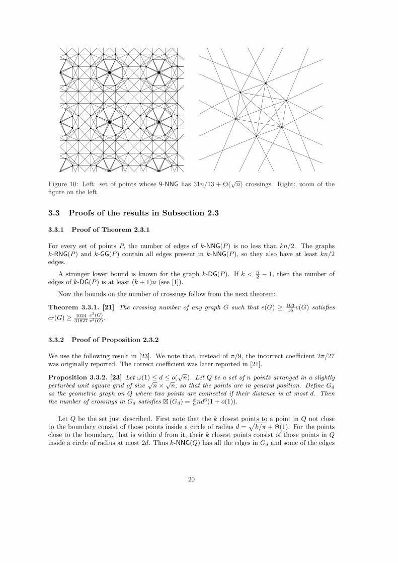
Figure 10: Left: set of points whose 9-NNG has 31n/13 + Θ(√

n) crossings. Right: zoom of thefigure on the left.

3.3 Proofs of the results in Subsection 2.3

3.3.1 Proof of Theorem 2.3.1

For every set of points P, the number of edges of k-NNG(P ) is no less than kn/2. The graphsk-RNG(P ) and k-GG(P ) contain all edges present in k-NNG(P ), so they also have at least kn/2edges.

A stronger lower bound is known for the graph k-DG(P ). If k < n2 − 1, then the number of

edges of k-DG(P ) is at least (k + 1)n (see [1]).

Now the bounds on the number of crossings follow from the next theorem:

Theorem 3.3.1. [21] The crossing number of any graph G such that e(G) ≥ 10316 v(G) satisfies

cr(G) ≥ 102431827

e3(G)v2(G) .

3.3.2 Proof of Proposition 2.3.2

We use the following result in [23]. We note that, instead of π/9, the incorrect coefficient 2π/27was originally reported. The correct coefficient was later reported in [21].

Proposition 3.3.2. [23] Let ω(1) ≤ d ≤ o(√

n). Let Q be a set of n points arranged in a slightlyperturbed unit square grid of size

√n × √n, so that the points are in general position. Define Gd

as the geometric graph on Q where two points are connected if their distance is at most d. Thenthe number of crossings in Gd satisfies £ (Gd) = π

9 nd6(1 + o(1)).

Let Q be the set just described. First note that the k closest points to a point in Q not closeto the boundary consist of those points inside a circle of radius d =

√k/π + Θ(1). For the points

close to the boundary, that is within d from it, their k closest points consist of those points in Qinside a circle of radius at most 2d. Thus k-NNG(Q) has all the edges in Gd and some of the edges

20

Figure 11: Point set whose 10-NNG has 4n + Θ(√

n) crossings.

in G2d whose endpoints are within d of the boundary. Thus

£ (k-NNG(Q)) ≤ π

9nd6(1 + o(1)) +

(π

9n(2d)6(1 + o(1))− π

9(√

n− 2d)2(2d)6(1 + o(1)))≤

≤ π

9nd6(1 + o(1)) + Θ(

√nd7) =

π

9nd6(1 + o(1)) =

19π2

k3n(1 + o(1)).

Except for a similar analysis for the points close to the boundary, two points in Q are neighbors

in k-RNG(Q) if their distance is at most d =√

k/(2π/3−√3/2) + Θ(1). Similarly, two points are

neighbors in k-GG(Q) or in k-DG(Q) if their distance is at most d = 2√

k/π. The result follows bythe Proposition and by noting that the extra crossings caused by the points close to the boundaryare at most o(nd6).

3.3.3 Proof of Theorem 2.3.3

Let e be an edge of k-DG(P ). Let us see that there are many edges in k-DG(P ) that do not cross e.

For the sake of simplicity, let us assume that e is horizontal. The line extending e divides Pminus the endpoints of e into two groups. Let Pa and Pb respectively denote the set of points aboveand below the line. We set |Pa| = l. Observe that |Pb| = n− l − 2.

Let us first assume that |Pa| ≥ k + 2 and |Pb| ≥ k + 2. Let p1, p2, . . . , pl denote the points in Pa

sorted from top to bottom. If i ∈ [2, k+2] and j ∈ [1, i−1], then pi is adjacent to pj in k-DG(P ). Itsuffices to consider the circle through pi and pj tangent to the horizontal line containing pi. Fromall points in P , this circle can only contain {p1, p2, . . . , pi−1} \ {pj} in its interior. Notice that theedges pip1, pip2, . . . , pipi−1 do not cross e.

If i ∈ [k + 3, l], we consider the same family of circles. More precisely, we consider a circletangent to the horizontal line through pi growing until its interior contains k + 1 points from Pa

(it could happen that the interior of the circle goes from having k points from Pa to having k + 2points from Pa; this case is similar). Then in k-DG(P ) these k + 1 points are connected to pi andall these edges do not cross e.

In conclusion, there exist (k + 1)(k + 2)/2 + (l− (k + 2))(k + 1) edges between points in Pa notcrossing e. By analogous arguments, there exist (k +1)(k +2)/2+ (n− l− 2− (k +2))(k +1) edges

21

between points in Pb not crossing e. This adds up to a total number of (k + 1)(n− k − 4) edges.

It remains to settle the case where either |Pa| < k + 2 or |Pb| < k + 2. Let us suppose that|Pa| < k + 2; since k < n/2 − 1, we have that |Pb| ≥ k + 1. Arguing as in the previous case, wefind (l − 1)l/2 + (k + 1)(k + 2)/2 + (n− l − 2− (k + 2))(k + 1) edges that do not cross e. It is notdifficult to see that, for any l < k + 2, this number is always greater than (k + 1)(n− k − 4).

In summary, since k-DG(P ) contains at most 3(k+1)n−3(k+1)(k+2) edges, e crosses no morethan 3(k + 1)n− 3(k + 1)(k + 2)− 1− (k + 1)(n− k − 4) edges in k-DG(P ). Hence the number ofcrossings of k-DG(P ) is upper bounded by 1

2 (3(k + 1)n− 3(k + 1)(k + 2)) (3(k + 1)n− 3(k + 1)(k +2)− 1− (k + 1)(n− k − 4)).

3.3.4 Proof of Proposition 2.3.4

Refer to Figure 12 (left). The upper chain contains n − k − 1 points on a circle C such that thedistance between consecutive points is constant. Let qi, qi+1 be two such consecutive points. Letl be the line through qi+1 perpendicular to −−−→qiqi+1, and let d be the distance between l and thecenter of C. The lower chain forms a convex chain seen from the upper chain and contains k + 1points that are at distance less than d from the center of C. This ensures that the closed diskwith diameter given by qi and some point from the lower chain does not contain any point fromthe upper chain different from qi. Thus in k-GG(Q) each point from the upper group is adjacent toeach point from the lower group. Notice that the construction can be perturbed to attain generalposition.

3.3.5 Proof of Proposition 2.3.5

Refer to Figure 12 (right). The number of points in the upper group is k + 1, and the lower groupcontains the same number of points. The rest of points are placed in the middle group. In k-DG(Q)each point qi in the middle group is connected to all upper and lower points, as it suffices to considerfamilies of increasing circles through qi with center at the vertical line through qi. This constructioncan be perturbed so that it becomes non-degenerate.

Figure 12: Left: set of points whose k-GG has k2n2/4 + o(k2n2) crossings. Right: set of pointswhose k-DG has k2n2/2 + o(k2n2) crossings.

3.3.6 Proof of Theorem 2.3.6

Lemma 3.3.3. In any angular sector with apex p ∈ P and amplitude α ≤ π/3, the only points thatcan be connected to p in the graph k-RNG(P ) are the k + 1 closest points to p that are contained inthe sector.

22

Proof. Let p1, p2, . . . be the points of P that are contained in the sector sorted by increasing distanceto p. For each i ≥ 2, the points p1, p2, . . . , pi−1 are contained in the intersection of the two diskscentered at p, pi with radius |ppi| (see Figure 13, left). Consequently, p and pi are not connectedin k-RNG(P ) if i− 1 > k.

Let e = pipj be an edge in k-RNG(P ). We define the lens associated to e as the open intersectionof the circles centered at pi and pj with radius |pipj |∗.

Now let us define a charging scheme that assigns every crossing in k-RNG(P ) to each of the twoinvolved edges e satisfying that at least one of the endpoints of the other edge is contained in thelens associated to e. Since each crossing defines a quadrilateral having at least one obtuse angle,the crossing is (at least) assigned to the edge opposite to this angle.

Let e be an edge in k-RNG(P ). The lens associated to e contains at most k points in P. ByLemma 3.3.3, each of them is adjacent to no more than 3k + 3 points in P such that the edge thatconnects them crosses e. Consequently, at most 3k2 + 3k crossings may be assigned to e.

Since each vertex in P has degree at most 6k + 6 (see Lemma 3.3.3), the number of edges ofk-RNG(P ) does not exceed 3kn + 3n, which yields the theorem.

3.3.7 Proof of Theorem 2.3.7

The proof of Theorem 2.3.7 requires several technical lemmas. The first one is a corollary ofLemma 3.3.3:

Lemma 3.3.4. In any angular sector with apex p ∈ P and amplitude α ≤ π/3, the only points thatcan be connected to p in the graph k-NNG(P ) are the k closest points to p that are contained in thesector.

Lemma 3.3.5. Let pi, pj , pl, pm be four elements of P, with |pipj | < |pipl| < |pipm|. If pjpm crossespipl, then |pjpl| < |pjpm|.

Proof. Let Ci,l and Cj,l respectively be the circles centered at pi and pj containing pl in theboundary (see Figure 13, middle). These circles have a non empty intersection and, since pi, pj ,and pl are not aligned, Ci,l is not contained in Cj,l, nor Cj,l is contained in Ci,l. Let q be theintersection point between Ci,l and the ray starting at pj and passing through pi. We have that|pjq| > |pjpl|. Therefore the ray starting at pj and passing through pi intersects Cj,l before Ci,l.This property is maintained for all rays starting at pj and contained in the wedge induced by theangle ∠pipjpl. In particular, it is maintained for the ray starting at pj and containing pm. Sincepm lies outside Ci,l, pm is not contained in Cj,l, so |pjpl| < |pjpm|.

Lemma 3.3.6. Let pi, pj , pl be three elements of P, with |pipj | < |pipl|. Then all points pm suchthat pjpm crosses pipl, |pipl| < |pipm|, |pmpi| > |pmpj |, and |pmpl| > |pmpj | are contained in anangular sector with apex pi and amplitude at most π/3.

Proof. Without loss of generality, we assume that the line through pi and pl is vertical, pi is abovepl, and pj is to the left of this line. The other situations are symmetric.

Let C be the circle centered at pi and containing pl in the boundary. Let li,j and lj,l respec-tively be the bisectors of pipj and pjpl. A point pm satisfying the hypothesis of the lemma lie onthe intersection R of the following four regions: the exterior of C, the semiplane opposite to pi

∗Unfortunately, it is standard in the computational geometry literature that a lens is incorrectly called a lune.

23

r

pi

pl

pj

C

q t

t′

R

li,j

lj,l

p

piα pi pl

pm

pj

Ci,l

Cj,l

q

Figure 13: Left: an angular sector with apex p and amplitude α ≤ π/3. Middle: four pointssatisfying the hypothesis of Lemma 3.3.5. Right: the region R in Lemma 3.3.6.

determined by li,j , the semiplane opposite to pl determined by lj,l, and the wedge induced by theangle ∠pipjpl (see Figure 13, right).

If pj has greater or equal ordinate than pi, it is not difficult to see that region R is empty.Observe that R is also empty if li,j or lj,l do not intersect the arc of C determined by the wedgeinduced by ∠pipjpl. Therefore the lemma clearly holds in these cases.

Let us now suppose that pj has smaller ordinate than pi, li,j intersects the arc of C determinedby the wedge induced by ∠pipjpl in a point q, and lj,l intersects the arc of C determined by thewedge induced by ∠pipjpl in a point r. Let t be the intersection of li,j and lj,l. In order for R notto be empty t must lie outside C. Let us assume that we are in this situation.

Consider the wedge formed by the ray starting at pj and passing through q together with theray starting from pj and passing through r. Observe that R is contained in this wedge. We willend the proof by showing that this wedge has angle at most π/3. Let t′ be the intersection of thebisector of pipl with the the arc of C determined by the wedge induced by ∠pipjpl. Notice that∠pjpiq > ∠pjpit

′ > ∠plpit′. By analogous arguments, ∠pjplr > ∠piplt

′. Since ∠plpit′ and ∠piplt

′

are angles of the equilateral triangle formed by pi, pl, and t′, then ∠pjpiq and ∠pjplr are greaterthan π/3. This implies that ∠pipjq and ∠plpjr are greater than π/3, since ∠pjpiq = ∠pipjq and∠plpjr = ∠pjplr. Given that ∠pipjq + ∠qpjr + ∠rpjpl < π, we conclude that ∠qpjr < π/3.

Now we are ready to prove Theorem 2.3.7.

Consider two crossing edges in k-NNG(P ) involving vertices pi, pj , pl, pm. We assign the crossingto each of the pairs of edges {−−→pipl,

−−→pipj} satisfying: (i) one of the two crossing edges is −−→pipl; (ii)|pipj | < |pipl| (so −−→pipj ∈ E(k-NNG(P ))).

Let us show that this assignment is consistent. The quadrilateral defined by the vertices involvedin the crossing has at least one obtuse angle. Then the crossing is assigned to the pair of directededges consisting of the edge opposite to this obtuse angle (which is a diagonal of the quadrilateral)and one edge with the same origin and lying in one side of the quadrilateral.

We devise a charging scheme that divides the weight of each crossing by the number of pairs ofedges the crossing is assigned to. We say that a crossing is simple if it is only assigned to one pairof edges, and we say that it is multiple otherwise. In the following we find the maximum weightthat a pair of edges can receive.

Let pj and pl be two of the k nearest neighbors of pi, with |pipj | < |pipl|. Each crossing assignedto {−−→pipl,

−−→pipj} can be associated with a vertex adjacent to pj in k-NNG(P ) (the fourth point involvedin the crossing). We want to bound the maximum number of such vertices. Let w be the wedge

24

induced by ∠pipjpl. If w has amplitude at most 2π/3, then, by Lemma 3.3.4, the maximum numberof crossings that may be assigned to {−−→pipl,

−−→pipj} is 2k. Otherwise we partition w into three wedgesw1, w2, and w3 as follows: w1 is bounded by the half-line with origin at pj and direction givenby −−→pjpi and has amplitude pi/3; w3 is bounded by the half-line with origin at pj and directiongiven by −−→pjpl and has amplitude pi/3; w2 consists of the part of w not covered by w1 and w3. Forν ∈ {1, 2, 3}, let nν be the number of vertices in wν that create a crossing assigned to {−−→pipl,

−−→pipj}.A direct application of Lemma 3.3.4 yields that nν ≤ k for ν ∈ {1, 2, 3}. Furthermore, since pi

is a point in w1 adjacent to pj , we have that n1 ≤ k − 1. Finally, consider the k closest pointsto pj contained in w3, which, by Lemma 3.3.4, are the only candidates to be connected to pj ink-NNG(P ). Observe that pl belongs to this set: otherwise, by Lemma 3.3.5, there would be k pointspm such that |pipl| > |pipm|, which is absurd because −−→pipl ∈ E(k-NNG(P )). Thus n3 ≤ k − 1. Inconclusion, the maximum number of crossings that may be assigned to {−−→pipl,

−−→pipj} is 3k − 2.

Next we analyze the maximum number of simple crossings that may be assigned to {−−→pipl,−−→pipj}.

Let pm be a vertex in P such that the edge pjpm (with some orientation) causes a crossing assignedto {−−→pipl,

−−→pipj}. If |pipm| < |pipl|, then the crossing is also assigned to {−−→pipl,−−→pipm}. If |pipm| > |pipl|

and −−−→pjpm ∈ E(k-NNG(P )), then, by Lemma 3.3.5, |pjpl| < |pjpm| and the crossing is also assignedto {−−−→pjpm,−−→pjpl}. If |pipm| > |pipl|, −−−→pmpj ∈ E(k-NNG(P )), and |pmpj | > |pmpi| or |pmpj | > |pmpl|,then the crossing is also assigned to {−−−→pmpj ,

−−→pmpi} or {−−−→pmpj ,−−→pmpl}. Therefore three necessary

conditions for pm to cause a simple crossing assigned to {−−→pipl,−−→pipj} are: (i) |pipm| > |pipl|; (ii)−−−→pmpj ∈ E(k-NNG(P )); (iii) |pmpi| > |pmpj | and |pmpl| > |pmpj |. By Lemmas 3.3.6 and 3.3.4, there

are at most k such points.

To conclude, in the worst case k simple crossings and 2k−2 crossings of weight 1/2 are assignedto {−−→pipl,

−−→pipj}. Thus any pair of edges in k-NNG(P ) receives weight at most 2k − 1.

3.3.8 Proof of Proposition 2.3.8

Consider the set Q = {q1, q2, . . . , qn}, where qi = (2i, 0). Let us slightly perturb the configurationso that the points are in convex position. The k nearest neighbors of each point qi such that i > kare qi−1, qi−2, . . . , qi−k. Therefore, if i ∈ [k + 1, n − k], then qi is connected in k-NNG(Q) to its kpredecessors and k successors in the “line”.

Let −−→qiqj , −−→qlqm be two crossing edges such that j < m < i < l. We assign this crossing to qj . Sup-pose that j ∈ [k+1, n−k]. Then the crossings between−−→qiqj and the following edges are assigned to qj :−−−−−→qj+1qj−1,

−−−−−→qj+2qj−1, . . . ,−−−−−−−→qj+k−1qj−1,

−−−−−→qj+1qj−2,−−−−−→qj+2qj−2, . . . ,

−−−−−−−→qj+k−2qj−2, . . . ,−−−−−→qj+1qi+1,

−−−−−→qj+2qi+1, . . . ,−−−−−−−→qi+k+1qi+1. This adds up to∑k−1

ν=i+k+1−j ν crossings. Since i might take values from j−k to j− 2,the total number of crossings assigned to qj is

j−2∑

i=j−k

k−1∑

ν=i+k+1−j

ν =k−1∑ν=1

ν2 =k3

3− k2

2+

k

6.

Given that j is an index in [k+1, n−k], the preceding charging scheme guarantees that k-NNG(Q)contains (n− 2k)

(k3/3− k2/2 + k/6

)crossings. Notice that the crossings we have not account for

in this argument have order o(k3n).

References

[1] M. Abellanas, P. Bose, J. Garcıa, F. Hurtado, C. M. Nicolas, and P. Ramos. On structuraland graph theoretic properties of higher order Delaunay graphs. Internat. J. Comput. Geom.Appl., 19(6):595–615, 2009.

25

[2] B. M. Abrego, M. Cetina, S. Fernandez-Merchant, J. Leanos, and G. Salazar. 3-symmetricand 3-decomposable drawings of Kn. Discrete Appl. Math., to appear.

[3] B. M. Abrego, S. Fernandez-Merchant, J. Leanos, and G. Salazar. A central approach tobound the number of crossings in a generalized configuration. Electron. Notes Discrete Math.,30:273–278, 2008.

[4] M. Ajtai, V. Chvatal, M. M. Newborn, and E. Szemeredi. Crossing-free subgraphs. Ann.Discrete Math., 12:9–12, 1982.

[5] G. Di Battista, P. Eades, R. Tamassia, and I. G. Tollis. Graph Drawing: Algorithms for theVisualization of Graphs. Prentice Hall, 1998.

[6] P. Brass, W. Moser, and J. Pach. Graph drawings and geometric graphs. Chapter in ResearchProblems in Discrete Geometry, pp. 373–416. Springer, 2005.

[7] R. O. Duda, P. E. Hart, and D. G. Stork. Pattern Classification. John Wiley & Sons, 2001.

[8] V. Dujmovic, K. Kawarabayashi, B. Mohar, and D. R. Wood. Improved upper bounds on thecrossing number. Proc. SoCG ’08, 375–384, 2008.

[9] M. R. Garey and D. S. Johnson. Crossing number is NP-complete. SIAM J. Algebra Discr.,4:312–316, 1983.

[10] J. Gudmundsson, M. Hammar, and M. van Kreveld. Higher order Delaunay triangulations.Comput. Geom., 23:85–98, 2002.

[11] R. K. Guy. A combinatorial problem. Bull. Malayan Math. Soc., 7:68–72, 1960.

[12] I. Herman, G. Melancon, and M. S. Marshall. Graph visualization and navigation in informa-tion visualization: A survey. IEEE T. VLSI Syst., 6:24–43, 2000.

[13] J. W. Jaromczyk and G. T. Toussaint. Relative neighborhood graphs and their relatives. Proc.IEEE, 80(9):1502–1517, 1992.

[14] M. Junger and P. Mutzel. Graph Drawing Software. Springer-Verlag, 2004.

[15] E. de Klerk, D. V. Pasechnik, and A. Schrijver. Reduction of symmetric semidefinite programsusing the regular ∗-representation. Math. Program., Ser. B, 109:613–624, 2007.

[16] M. van Kreveld, M. Loffler, and R. I. Silveira. Optimization for first order Delaunay triangu-lations. Comput. Geom., 43(4):377–394, 2010.

[17] F. T. Leighton. Complexity Issues in VLSI. MIT Press, 1983.

[18] G. Liotta. Proximity drawings. Chapter in Handbook of Graph Drawing and Visualization.Chapman & Hall/CRC Press, in preparation.

[19] A. Okabe, B. Boots, K. Sugihara, and S. N. Chiu. Spatial Tessellations: Concepts and Appli-cations of Voronoi Diagrams. John Wiley & Sons, 2000.

[20] J. Pach, ed. Towards a Theory of Geometric Graphs. Amer. Math. Soc., 2004.

[21] J. Pach, R. Radoicic, G. Tardos, and G. Toth. Improving the crossing lemma by finding morecrossings in sparse graphs. Discrete Comput. Geom., 36:527–552, 2006.

[22] J. Pach, J. Spencer, and G. Toth. New bounds on crossing numbers. Discrete Comput. Geom.,24:623–644, 2000.

26

[23] J. Pach and G. Toth. Graphs drawn with few crossings per edge. Combinatorica, 17(3):427–439, 1997.

[24] T.-H. Su and R.-Ch. Chang. The K-Gabriel graphs and their applications. Proc. SIGAL’90.LNCS, vol. 450, pp. 66–75. Springer, 1990.

[25] T.-H. Su and R.-Ch. Chang. Computing the k-relative neighborhood graphs in Euclideanplane. Pattern Recogn., 24:231–239, 1991.

[26] G. Toussaint. Geometric proximity graphs for improving nearest neighbor methods in instance-based learning and data mining. Internat. J. Comput. Geom. Appl., 15(2):101–150, 2005.

[27] P. Turan. On an extremal problem in graph theory. Matematicko Fizicki Lapok, 48:436–452,1941.

[28] D. R. Wood and J. A. Telle. Planar decompositions and the crossing number of graphs withan excluded minor. New York J. Math., 13:117–146, 2007.

[29] K. Zarankiewicz. On a problem of P. Turan concerning graphs. Fund. Math., 41:137–145, 1954.

27