On Control under Communication Constraints in Autonomous...
112
On Control under Communication Constraints in Autonomous Multi-robot Systems ALBERTO SPERANZON Licentiate Thesis Stockholm, Sweden 2004
Transcript of On Control under Communication Constraints in Autonomous...
On Control under Communication Constraints inAutonomous Multi-robot Systems
ALBERTO SPERANZON
Licentiate ThesisStockholm, Sweden 2004
TRITA-S3-REG-0403ISSN 1404-2150ISBN 91-7283-885-X
KTH Signals, Sensors and SystemsSE-100 44 Stockholm
SWEDEN
Academic thesis, which with the approval of Kungliga Tekniska Hogskolan, will bepresented for public review in fulfillment of the requirements for a Licentiate ofEngineering in Automatic Control. The public review will be held on 2004/11/12at Royal Institute of Technology, Stockholm, Room V2, Teknikringen 76.
c© Alberto Speranzon, 2004
Tryck: Universitetsservice US AB
iii
Abstract
Multi-robot systems have important applications, such as space explorations, un-derwater missions, and surveillance operations. In most of these cases robots needto exchange data through communication. Limitations in the communication sys-tem however impose constraints on the design of coordination strategies. In thisthesis we present three papers on cooperative control problems in which differentcommunication constraints are considered.
The first paper describes a rendezvous problem for a team of robots that ex-changes position information through communication. A local control law for eachrobot should steer the team to a common meeting point when communicated dataare quantized. The robots are not equipped with any sensors so the positions ofother teammates are not measured. Two different types of quantized communi-cation are considered: uniform and logarithmic. Logarithmic quantization is oftenpreferable since it requires that fewer bits are communicated compared to when uni-form quantization is used. For a class of feasible communication topologies, controllaws that solve the rendezvous problem are derived.
A hierarchical control structure is proposed in the second paper, for modellingautonomous underwater vehicles employed in finding a minimum of a scalar field.The controller is composed of two layers. The upper layer is the team controller,which is modeled as discrete-event system. It generates waypoints based on thesimplex search optimization algorithm. The waypoints are used as target pointsby the lower control layer, which continuously steers each vehicle from the currentto the next waypoint. It is shown that the communication of measurements isneeded at each step for the team controller to generate unique waypoints. A protocolis proposed to reduce the amount of data to be exchanged, motivated by thatunderwater communication is costly in terms of energy.
In the third paper, a probabilistic pursuit–evasion game is considered as an ex-ample to study constrained communication in multi-robot systems. This system canbe used to model search-and-rescue operations and multi-robot exploration. Com-munication protocols based on time-triggered and event-triggered synchronizationschemes are considered. It is shown that by limiting the communication to eventswhen the probabilistic map updated by the individual pursuer contains new infor-mation, as measured by a map entropy, the utilization of the communication linkcan be considerably improved compared to conventional time-triggered communi-cation.


v
Acknowledgements
First of all I would like to thanks my supervisor Karl Henrik Johansson for hisguidance, inspiring discussions and support throughout my research. Without hisnever ending patience this thesis would probably not exists today.
I owe my gratitude to Bo Wahlberg who accepted me as a graduate studentat the Automatic Control Group. He also gave valuable comments on the thesismanuscript. I am also particularly grateful to Mikael Johansson, who has read andcommented several parts.
The main part of the thesis consists in three papers. I am indebted to the coau-thors of these. They are stated on the first page of each paper and their affiliationis included in the first chapter of the thesis. The coauthors are Fabio Fagnani, KarlHenrik Johansson, Jorge Silva, Joao Borges de Sousa and Sandro Zampieri.
I would like to thanks Joao Pedro Hespanha for introducing me to the problemon probabilistic pursuit–evasion games during his short visit at KTH.
I am grateful to Shankar Sastry and Rene Vidal for providing the photo ofan experiment on pursuit–evasion, Joao de Sousa for the photo of the underwatervehicle, and Paul S. Schenker for the photo of the collaborative platforms of JPL.
I would like to take the opportunity to thank Henning Schmidt and JochenGiese for all the interesting discussions we had, not only about research.
To all the friends I met here in Stockholm, who have given me many greatmoments far away from robots and control systems: thank you.
Special thanks go to my family in Italy whose love and support made the distancebetween us appear much less than it really is.
Most of all I would like to thank my wife Jovita for her continuous presence,support and encouragement. I must express my adoration of my daughter, Alice,who is the greatest joy of our life.
The research described in this thesis has been sponsored by the European Com-mission through the RECSYS project IST-2001-32515 and the Swedish ResearchCouncil. The support is gratefully acknowledged.


Contents
Contents vii
1 Introduction 3
1.1 Multi-robot systems under communication constraints . . . . . . . . 3
1.2 Motivating examples . . . . . . . . . . . . . . . . . . . . . . . . . . . 5
1.3 Main contributions of the thesis . . . . . . . . . . . . . . . . . . . . . 7
1.4 Remark on notation . . . . . . . . . . . . . . . . . . . . . . . . . . . 10
1.5 Other publications . . . . . . . . . . . . . . . . . . . . . . . . . . . . 10
1.6 Affiliation of the coauthors of the papers in the thesis . . . . . . . . 11
References . . . . . . . . . . . . . . . . . . . . . . . . . . . . . . . . . . . . 13
I Background 15
2 Control under communication constraints 17
2.1 Digital communication system . . . . . . . . . . . . . . . . . . . . . . 17
2.2 Communication limitations in the control problem . . . . . . . . . . 21
3 Autonomous multi-robot systems 27
3.1 Single-robot models . . . . . . . . . . . . . . . . . . . . . . . . . . . 27
3.2 Multi-robots mathematical model . . . . . . . . . . . . . . . . . . . . 31
4 Multi-robot systems with communication constraints 35
4.1 Team decision theory . . . . . . . . . . . . . . . . . . . . . . . . . . . 36
4.2 Consensus problems . . . . . . . . . . . . . . . . . . . . . . . . . . . 39
4.3 Towards a theory for multi-robot systems . . . . . . . . . . . . . . . 40
References 44
vii

viii Contents
II Papers 45
5 Paper A: On Multi-Vehicle Rendezvous Under Quantized Com-munication 475.1 Introduction . . . . . . . . . . . . . . . . . . . . . . . . . . . . . . . . 495.2 Problem formulation . . . . . . . . . . . . . . . . . . . . . . . . . . . 495.3 Two-vehicles rendezvous . . . . . . . . . . . . . . . . . . . . . . . . . 525.4 n-vehicles rendezvous . . . . . . . . . . . . . . . . . . . . . . . . . . . 565.5 Simulation results . . . . . . . . . . . . . . . . . . . . . . . . . . . . 595.6 Conclusions . . . . . . . . . . . . . . . . . . . . . . . . . . . . . . . . 59References . . . . . . . . . . . . . . . . . . . . . . . . . . . . . . . . . . . . 65
6 Paper B: Hierarchical control architecture for a team of under-water vehicles in search missions 676.1 Introduction . . . . . . . . . . . . . . . . . . . . . . . . . . . . . . . . 696.2 Hierarchical multi-vehicle model . . . . . . . . . . . . . . . . . . . . 706.3 Team controller . . . . . . . . . . . . . . . . . . . . . . . . . . . . . . 726.4 Communication issues . . . . . . . . . . . . . . . . . . . . . . . . . . 766.5 Vehicle controller . . . . . . . . . . . . . . . . . . . . . . . . . . . . . 786.6 Simulation . . . . . . . . . . . . . . . . . . . . . . . . . . . . . . . . . 796.7 Conclusions . . . . . . . . . . . . . . . . . . . . . . . . . . . . . . . . 80References . . . . . . . . . . . . . . . . . . . . . . . . . . . . . . . . . . . . 84
7 Paper C: On Some Communication Schemes for DistributedPursuit–Evasion Games 857.1 Introduction . . . . . . . . . . . . . . . . . . . . . . . . . . . . . . . . 877.2 Pursuit–Evasion with Communication . . . . . . . . . . . . . . . . . 877.3 Entropy-triggered synchronization . . . . . . . . . . . . . . . . . . . 897.4 Bandwidth limitations . . . . . . . . . . . . . . . . . . . . . . . . . . 917.5 Simulation results . . . . . . . . . . . . . . . . . . . . . . . . . . . . 937.6 Conclusions and future work . . . . . . . . . . . . . . . . . . . . . . 947.7 Acknowledgments . . . . . . . . . . . . . . . . . . . . . . . . . . . . . 95References . . . . . . . . . . . . . . . . . . . . . . . . . . . . . . . . . . . . 100
IIIConclusions 101
8 Conclusions and future work 103
List of Figures
1.1 Multi-robot application: search-and-rescue scenario. (Photograph pro-vided by courtesy of the Robotics and Intelligent Machines Laboratory,Berkeley, USA).[VSK+02]. . . . . . . . . . . . . . . . . . . . . . . . . . . 4
1.2 Multi-robot application: cooperative bar lifting. (Photograph providedby courtesy of Jet Propulsion Laboratory, Pasadena, USA). . . . . . . . 5
1.3 Example 1. Formation control. . . . . . . . . . . . . . . . . . . . . . . . 6
1.4 Example 2. Collaborative tracking. . . . . . . . . . . . . . . . . . . . . . 7
1.5 Example 3. Collaborative map building. . . . . . . . . . . . . . . . . . . 8
2.1 Block diagram of control systems interconnected via a communicationchannel. . . . . . . . . . . . . . . . . . . . . . . . . . . . . . . . . . . . . 18
2.2 General block diagram of a digital communication system. . . . . . . . . 19
2.3 Control system with communication channel modeled as random delay. 22
2.4 Control system with communication channel modeled as data drop (solidline). Data are dropped when the switch is in position 0. . . . . . . . . . 23
2.5 A 2D quantizer. Vi represents a quantization region and qi is the quan-tized value associated to the quantization region Vi. . . . . . . . . . . . 24
2.6 Two different types of quantizers: uniform and logarithmic. . . . . . . . 24
2.7 Control system with communication modeled as quantization. . . . . . . 25
3.1 Unicycle robot. . . . . . . . . . . . . . . . . . . . . . . . . . . . . . . . . 28
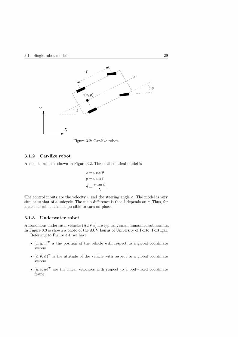
3.2 Car-like robot. . . . . . . . . . . . . . . . . . . . . . . . . . . . . . . . . 29
3.3 Underwater robot ISURUS. (Photograph provided by courtesy of theUnderwater Systems and Technology Laboratory, University of Porto,Portugal). . . . . . . . . . . . . . . . . . . . . . . . . . . . . . . . . . . . 30
3.4 Underwater robot. . . . . . . . . . . . . . . . . . . . . . . . . . . . . . . 31
3.5 Hierarchical controller . . . . . . . . . . . . . . . . . . . . . . . . . . . . 32
4.1 Multi-robot system with communication channels depicted. The solidarrows represent wireless communication channels and empty arrowsrepresent the sensor and actuation signals. The T/R blocks representthe transmitters and receivers of the digital communication systems. . . 36
4.2 Example of a partially nested information structure. . . . . . . . . . . . 38
1

2 List of Figures
4.3 Example of n = 11 robots in a formation control problem. The headingof the formation is the average of the single robot heading. . . . . . . . 39
5.4 For large quantization step δ the value of k1(δ) tends to zero. . . . . . . 555.5 Three different communication topologies for n = 3. Solid lines denote
uniformly quantized communication channels, and dashed lines logarith-mically quantized communication channels. . . . . . . . . . . . . . . . . 56
5.6 Trajectories for three vehicles for the three different topologies of fig-ure 5.5. In the simulations we assumed the uniform quantization errorequal to zero. . . . . . . . . . . . . . . . . . . . . . . . . . . . . . . . . . 62
5.7 Performance comparison of the difference communication topologies. . . 636.8 Autonomous Underwater Vehicle used in the PISCIS project at Porto
University. . . . . . . . . . . . . . . . . . . . . . . . . . . . . . . . . . . . 706.9 Hierarchical control structure for n vehicles. . . . . . . . . . . . . . . . . 716.10 A triangular grid with aperture d over a two-dimensional scalar field
depicted by its level curves. The solid line triangle illustrates the statez of the discrete-event system evolving on the grid. . . . . . . . . . . . . 73
6.11 Decentralized hierarchical control structure for n = 2 vehicles with acommunication channel. . . . . . . . . . . . . . . . . . . . . . . . . . . . 75
6.12 Motion of the AUV’s and communicated date for two different scenarios.In dotted line is shown the current simplex. With the arrowed solid line isrepresented the communication of raw measurement, while with a dashedline is represented the transmission of a message. In deash-dotted line isshown the trajectory of the AUV’s toward the destination vertexes. . . . 77
6.13 Trajectories of two AUV’s controlled by the hierarchical control algo-rithm proposed in the paper. . . . . . . . . . . . . . . . . . . . . . . . . 81
6.14 The figures show the simplex, the trajectories of the AUV’s and a movingscalar field at different time steps. The scalar field, shown through levelcurves, is a quadratic function with superimposed white noise. . . . . . 81
7.15 At a synchronization time τ ∈ T , each pursuer Pi broadcasts yi(τ) tothe network and receives Yi(τ) = yj(τ)j 6=i. . . . . . . . . . . . . . . . 90
7.16 Vector quantization K = Q(M) of probabilistic map M . . . . . . . . . . 927.17 Capture time T ∗ for hundred Monte Carlo experiments and the three
proposed synchronization schemes. The dashed line is the mean capturetimes T
∗and the dashed-dotted is line the standard deviations. The
map size is n2c = 242. . . . . . . . . . . . . . . . . . . . . . . . . . . . . . 95
7.18 Number of synchronization instances S for the same hundred MonteCarlo experiments as in Figure 7.17. . . . . . . . . . . . . . . . . . . . . 96
7.19 Capture time T ∗ for hundred Monte Carlo experiments. In this case thesize of the map is n2
c = 322. . . . . . . . . . . . . . . . . . . . . . . . . . 97
Chapter 1Introduction
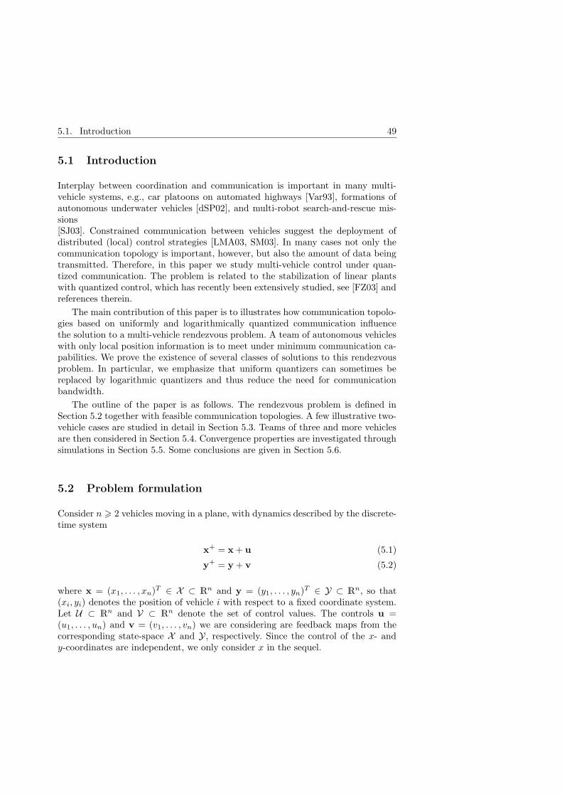
Strategies for multi-robot systems to perform particular tasks very often rely onthe presence of a communication network, which links the different components ofthe system. Limitations of such communication links impose constraints that mustbe taken into account in development of the strategies. The papers collected in thisthesis deal with the design of controllers when the task to be performed and thecommunication limitations are specifications of the problem.
The purpose of this introduction is to motivate the problems considered in thepapers. In the following we discuss the general problem of controlling a team ofrobots with communication limitations and three motivating examples are pre-sented. Summaries of the three papers and their main contributions are includedat the end of this chapter.
1.1 Multi-robot systems under communication constraints
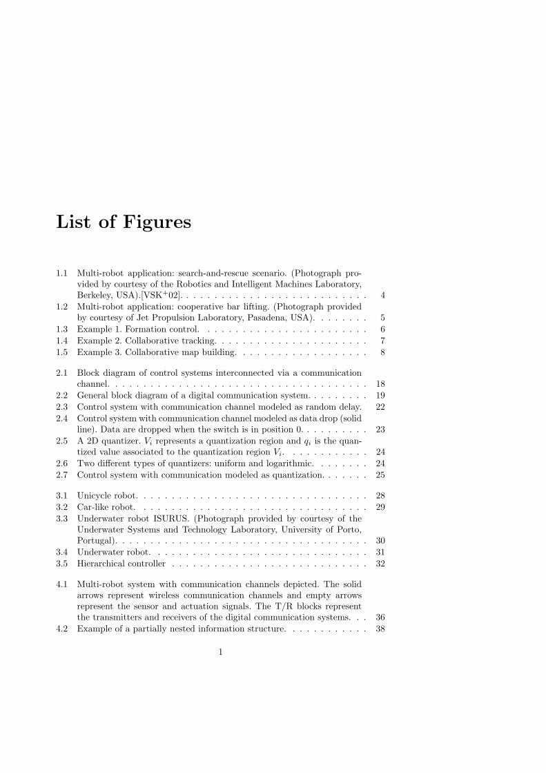
Over the past decade, a significant shift of focus has occurred in the field of mobilerobotics as researchers have begun to investigate problems involving many, ratherthan single, robots. Several new robotics application areas, such as underwater andspace exploration, service robotics in public and private domains can benefit fromthe use of multi-robot systems. Multi-robot systems can often deal with tasks thatare difficult, or even impossible, to be accomplished by an individual robot. A teamof robots may also provide redundancy, efficiency, cheaper deployment beyond whatis possible with single robots. Let us consider two typical applications of multi-robotsystems.
The first (see Figure 1.1) is a search-and-rescue operation where a team of robotsis deployed in an unknown or partially known hazardous environment, where ahuman being or an object should be found. As shown in Figure 1.1, a team ofground mobile robots equipped with sensors are coordinated, together with aerial
3
4 Chapter 1. Introduction
Figure 1.1: Multi-robot application: search-and-rescue scenario. (Photograph pro-vided by courtesy of the Robotics and Intelligent Machines Laboratory, Berkeley,USA).[VSK+02].
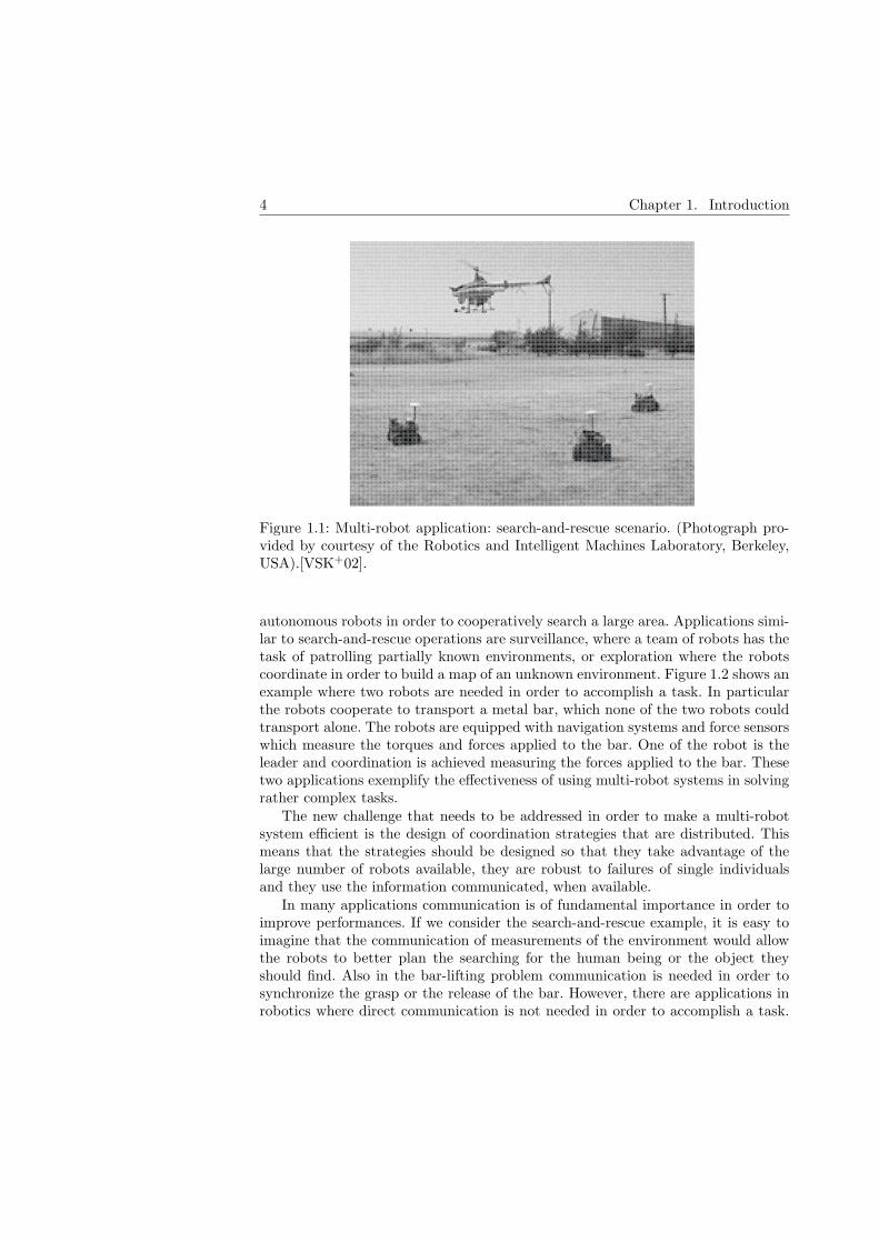
autonomous robots in order to cooperatively search a large area. Applications simi-lar to search-and-rescue operations are surveillance, where a team of robots has thetask of patrolling partially known environments, or exploration where the robotscoordinate in order to build a map of an unknown environment. Figure 1.2 shows anexample where two robots are needed in order to accomplish a task. In particularthe robots cooperate to transport a metal bar, which none of the two robots couldtransport alone. The robots are equipped with navigation systems and force sensorswhich measure the torques and forces applied to the bar. One of the robot is theleader and coordination is achieved measuring the forces applied to the bar. Thesetwo applications exemplify the effectiveness of using multi-robot systems in solvingrather complex tasks.
The new challenge that needs to be addressed in order to make a multi-robotsystem efficient is the design of coordination strategies that are distributed. Thismeans that the strategies should be designed so that they take advantage of thelarge number of robots available, they are robust to failures of single individualsand they use the information communicated, when available.
In many applications communication is of fundamental importance in order toimprove performances. If we consider the search-and-rescue example, it is easy toimagine that the communication of measurements of the environment would allowthe robots to better plan the searching for the human being or the object theyshould find. Also in the bar-lifting problem communication is needed in order tosynchronize the grasp or the release of the bar. However, there are applications inrobotics where direct communication is not needed in order to accomplish a task.

1.2. Motivating examples 5
Figure 1.2: Multi-robot application: cooperative bar lifting. (Photograph providedby courtesy of Jet Propulsion Laboratory, Pasadena, USA).
The transportation of the bar, when no grasping or releasing actions are needed, isan example.
In this thesis we will consider the design and analysis of distributed strategieswhen robots can exchange data. The presence of a communication network connect-ing robots, however, imposes limitations since data needs to be quantized to be sentover the network, it can be received with large delays due to bandwidth limitationsof the channels or it can be lost due to noise in the environment or because the net-work is congested, etc. Thus a new design problem arises: how do we design controlstrategies that coordinate a team of robots under communication constraints? Inthis thesis we presents three papers in which three different coordination problemsare considered under various communication constraints: quantization (Paper A),noisy channel (Paper B), bandwidth limitation (Paper C).
1.2 Motivating examples
We consider here three motivating examples which are related to the coordinationproblems addressed in the papers.
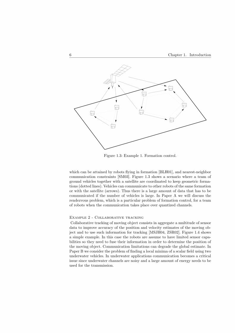
Example 1 - Formation control
Formation control problems arise in those applications where a team of robotshave to maintain specific geometries. The need of keeping specific formations couldbe motivated by sensor fusion constraints, as for example in a team of spacecraftsemployed to create a large interferometer [Lin03], energy consumption limitations,
6 Chapter 1. Introduction
Figure 1.3: Example 1. Formation control.
which can be attained by robots flying in formation [BLH01], and nearest-neighborcommunication constraints [SM03]. Figure 1.3 shows a scenario where a team ofground vehicles together with a satellite are coordinated to keep geometric forma-tions (dotted lines). Vehicles can communicate to other robots of the same formationor with the satellite (arrows). Thus there is a large amount of data that has to becommunicated if the number of vehicles is large. In Paper A we will discuss therendezvous problem, which is a particular problem of formation control, for a teamof robots when the communication takes place over quantized channels.
Example 2 - Collaborative tracking
Collaborative tracking of moving object consists in aggregate a multitude of sensordata to improve accuracy of the position and velocity estimates of the moving ob-ject and to use such information for tracking [MSJH04, ZSR02]. Figure 1.4 showsa simple example. In this case the robots are assume to have limited sensor capa-bilities so they need to fuse their information in order to determine the position ofthe moving object. Communication limitations can degrade the global estimate. InPaper B we consider the problem of finding a local minima of a scalar field using twounderwater vehicles. In underwater applications communication becomes a criticalissue since underwater channels are noisy and a large amount of energy needs to beused for the transmission.

1.3. Main contributions of the thesis 7
Figure 1.4: Example 2. Collaborative tracking.
Example 3 - Collaborative map building
Collaborative map building is another common problem for multi-robot systems, inwhich robots are employed in building a map of an unknown environment [FBKT00].In Figure 1.5 robots are deployed in a structured environment such as a house ora factory, and they exchange information in order to build a complete map. In thiscase it is crucial to consider the quantity of data transmitted over the network,because of bandwidth constraints and traffic congestion. In Paper C we discussproblems related to collaborative map building.
1.3 Main contributions of the thesis
This thesis contains the three papers listed below.
Paper A: On multi-vehicle rendezvous under quantized communication.
Multi-vehicle rendezvous can be considered as a formation control problem whereall members of the group eventually meet at a single unspecified location. In this pa-per we assume the vehicles do not perform any active sensing of the neighborhood,but they can exchange information through quantized communication channels. Wealso assume the vehicles can communicate with any other vehicle. In order to havean efficient utilization of the bandwidth some data is transmitted through logarith-mically quantized channels. We derive some communication topologies i.e., a graphassociated to the system that gives the type of quantized channel utilized betweenpairs of vehicles. We prove that for such communication topologies the relative dis-

8 Chapter 1. Introduction
PSfrag replacements
Complete Map
Local Map 1
Local Map 2
Local Map 3
Local Map 4
Local Map 5
Figure 1.5: Example 3. Collaborative map building.
tance between vehicles converges to a neighborhood of the origin.
Paper A is based on the following publications:
K. H. Johansson, A. Speranzon, and S. Zampieri: “On quantization and com-munication topologies in multi-vehicle rendezvous”. Submitted to 16th IFACWorld Congress, Prague, Czech Republic, 2005
F. Fagnani, K. H. Johansson, A. Speranzon, and S. Zampieri: “On multi-vehicle rendezvous under quantized communication”. International Sympo-sium on Mathematical Theory of Networks and Systems, Leuven, Belgium,2004
Paper B: On collaborative optimization and communication for a team of au-tonomous underwater vehicle.
A hierarchical control structure is proposed in the second paper, for modellingautonomous underwater vehicles employed in finding a minimum of a scalar field.The controller is composed of two layers. The upper layer is the team controllerwhich is modeled as discrete-event system. It generates waypoints based on thesimplex search optimization algorithm. The waypoints are used as target points bythe lower control layer, which continuously steer each vehicle from the current tothe next waypoint. It is shown that the communication of measurements is needed

1.3. Main contributions of the thesis 9
at each step for the team controller to generate unique waypoints. A protocol isproposed to reduces the amount of data to be exchanged, motivated by that under-water communication is costly in terms of energy.
Paper B is based on the following publications:
J.B. de Sousa, K.H. Johansson, A. Speranzon, and J. Silva: “A control archi-tecture for multiple submarines in coordinated search missions”. Submitted to16th IFAC World Congress, Prague, Czech Republic, 2005
J. Silva, A. Speranzon, J.B. de Sousa, and K. H. Johansson: “Hierarchicalsearch strategy for a team of autonomous vehicles”, International Symposiumon Intelligent Autonomous Vehicles, Lisbon, 2004
A. Speranzon, J. Silva, J.B. de Sousa, and K. H. Johansson: “On collabora-tive optimization and communication for a team of autonomous underwatervehicles”, Reglermote, Gothenburg, 2004.
Paper C: On some communication schemes for distributed pursuit–evasion games.
Pursuit–evasion game is a typical problem in game theory that can be used as modelfor multi-robot search-rescue problems, exploration, etc. In this paper we considerthe probabilistic set-up introduced by Hespanha et al. [HKS99] where all pursuerscontributes to build a global probabilistic map, which is the probability of the evaderto be in one of the possible cells the environment has been divided in, given all themeasurements taken by all pursuers. Such model is extended and made distributed.Each pursuer builds a local probabilistic map which is communicated with otherpursuers (synchronized) only when enough information has been collected by eachpursuers. We compare two possible communication strategies: periodic communi-cation and event-based communication. The event that triggers the communicationis the entropy of the probabilistic map i.e., the information content of the map.This idea can be related to the difference of periodic and event-based sampling.Communication of probabilistic maps with limited bandwidth is discussed in theend of the paper.
Paper C is based on the following publications:
A. Speranzon, and K. H. Johansson: “On some communication schemes fordistributed pursuit-evasion games”. IEEE Conference on Decision and Con-trol, Maui, HI, 2003
A. Speranzon, and K. H. Johansson: “Distributed pursuit-evasion game: eval-uation of some communication schemes”. Symposium on Autonomous Intelli-gent Networks and Systems. Menlo Park, CA, 2003

10 Chapter 1. Introduction
A. Speranzon, and K. H. Johansson: “On localization and communicationissues in pursuit-evasion game”. IROS, Workshop on Cooperative Robotics.Lausanne, Switzerland, 2002
1.4 Remark on notation
The thesis consists of three separated papers, therefore the notation throughout thethesis in not consistent, but is introduced separately in each paper.
1.5 Other publications
The author of the thesis has been co-author of other publications in the field ofrobotics and automatic control and some have influenced the contents of this thesis.They include the following:
M. Mazo, A. Speranzon, K.H. Johansson, X. Hu: “Multi-robot tracking of amoving object using directional sensors”. IEEE International Conference onRobotics and Automation, 2004.
E. Pagello, A. D’Angelo, C. Ferrari, R. Polesel, R. Rosati, A. Speranzon:“Emergent behaviors of a robot team performing cooperative tasks”. AdvancedRobotics, Vol. 15, No. 1, 3-20, 2003.
C. Altafini, A. Speranzon, K.H. Johansson: “Hybrid Control of a Truck andTrailer Vehicle”. In Hybrid Systems: Computation and Control, C.J. Tomlinand M.R. Greenstreet, Ed. - Lecture Notes in Computer Science, Springer-Verlag. 2002.
P. de Pascalis, M. Ferraresso, M. Lorenzetti, A. Modolo, M. Peluso, R. Polesel,R. Rosati, N. Scattolin, A. Speranzon, W. Zanette: “Golem Team in Middle-Sized Robots League”. In RoboCup-2000: Robot Soccer World Cup IV, P.Stone, T. Balch, and G. Kraetszchmar, Ed. - Springer-Verlag, Berlin, 2001.
C. Altafini, A. Speranzon, B. Wahlberg: “A Feedback Control Scheme forReversing a Truck and Trailer Vehicle”. IEEE Transactions on Robotics andAutomation, Dec. 2001.
R. Polesel, R. Rosati, A. Speranzon, C. Ferrari, E. Pagello: “Using Colli-sion Avoidance Algorithms for Designing Multi-robot Emergent Behaviors”.IEEE/RSJ International Conference on Intelligent Robots and Systems, 2000.
1.6. Affiliation of the coauthors of the papers in the thesis 11
1.6 Affiliation of the coauthors of the papers in the thesis
Fabio FagnaniDipartimento di Matematica,Politecnico di Torino,Corso Duca degli Abruzzi 24,10129 Torino, [email protected]
Karl Henrik JohanssonRoyal Institute of TechnologyDept. of Signals, Sensors and SystemsQsquldas vag 10100-44 Stockholm, [email protected]
Jorge SilvaInstituto Superiorde Engenharia do Porto,Rua Dr. Antonio Bernardinode Almeida 431,4200-072 Porto, [email protected]
Joao B. De SousaFaculdade de Engenhariada Universidade do Porto,Rua Dr. Roberto Frias,44200-465 Porto, [email protected]
Sandro ZampieriDipartimento di Ingegneriadell’Informazione,Universita di Padova,via Gradenigo 6/A,35131 Padova, [email protected]


References
[BLH01] R.W. Beard, J. Lawton, and F.Y. Hadaegh. A coordination architecturefor spacecraft formation control. IEEE Transaction on Control SystemsTechnology, 9:777–790, 2001.
[FBKT00] D. Fox, W. Burgard, H. Kruppa, and S. Thrun. A probabilistic approachto collaborative multi-robot localization. Special issue of AutonomousRobots on Heterogeneous Multi-Robot Systems, 3, 2000.
[HKS99] J.P. Hespanha, H. J. Kim, and S. Sastry. Multiple-agent probabilisticpursuit–evasion games. In IEEE Conference on Decision and Control,volume 3, pages 2432–2437, 1999.
[Lin03] C.A. Lindensmith. Technology plan for the Terrestrial Planet Finder.Technical report, Jet Propulsion Laboratory, California Institute ofTechnology, Pasadena, California, 2003.
[MSJH04] M. Mazo, A. Speranzon, K.H. Johansson, and X. Hu. Multi-robot track-ing of a moving object using directional sensors. In IEEE InternationalConference on Robotics and Automation, 2004.
[SM03] R. O. Saber and R. M. Murray. Flocking with obstacle avoidance: co-operation with limited communication in mobile networks. In Proc. ofthe 42nd IEEE Conference on Decision and Control, HI, USA, 2003.
[VSK+02] R. Vidal, O. Shakernia, J. Kim, D. Shim, and S. Sastry. Probabilisticpursuit-evasion games: Theory, implementation and experimental eval-uation. IEEE Transactions on Robotics and Automation, 2002.
[ZSR02] F. Zhao, J. Shin, and J. Reich. Information-driven dynamic sensor col-laboration for tracking applications. IEEE Signal Processing Magazine,2002.
13


Part I
Background
15


Chapter 2Control under communication
constraints
“In control and communication we are always fighting nature’stendency to degrade the organized and to destroy the meaningful”
- N. Wiener
In recent years a certain interest has been developed on control problems in whichthe communication is an essential component [Mit01]. A block diagram of such asystem is shown in Figure 2.1. For these systems, control design objectives such asregulation, tracking, etc. need to be addressed considering the limitations imposedby communication channels linking the different components (cf. Figure 2.1).
In the following we describe in some detail the digital communication channelhighlighting the constraints that it imposes. We then discuss how such constraintscan be modeled from a control perspective in order to incorporate them in thedesign of controllers.
2.1 Digital communication system
A block diagram of a digital communication system is shown in Figure 2.2. Theproblem of communication is how to design the transmitter and receiver (shownin dashed line in Figure 2.2), so that symbols selected at the source can be repro-duced at the destination either exactly or approximately. The reason why it is adifficult problem is due to the presence of the noise η in the channel and bandwidthconstraints. The noise degrades the information sent over the channel and specificdesign of the transmitter and receiver are needed in order to reliably communicatesymbols. The noise comes from many different sources, such as thermal noise inthe components, interference or degradation due to signal attenuation, amplitude
17

18 Chapter 2. Control under communication constraints
PSfrag replacements
CommunicationChannel
Controller
ControllerControllerController
Plant
Plant
Plant
Figure 2.1: Block diagram of control systems interconnected via a communicationchannel.
and phase distortion or multi-path distortion, which is caused by the existence ofmore than one propagation path between the transmitter and the receiver. Band-width constraints are generally caused by physical limitations of the medium andelectronic components used to implement the different parts of the transmitter andreceiver.
We will review in the following the main properties, and limitation of a digitalcommunication
The source is modeled as a discrete-time stochastic process, Xn with alphabetX and probability mass function p(xn) = Pr[Xn = xn] for xn ∈ X . We also assumethat the random variables Xn are independent and identical distributed (i.i.d.)1.We assume that the source alphabet X has cardinality M .
The transmitter operates on the symbol in order to produce a signal compatiblewith the channel, adding some redundancy used at the receiver to correct possi-ble errors. The transmitter is composed of a source and channel encoder and amodulator.
For a digital memoryless communication system, a source encoder is defined asthe mapping2
c : X → D∗ : x 7→ c(x) (2.1)
where x is a realization of X The source codeword c(x) is a string of length m ofsymbols chosen from a discrete alphabet D with card(D) = d. The mapping c isusually chosen so that the symbol x is converted into a codeword c(x) that haslittle or no redundancy. Roughly speaking the M symbols produced by the sourceare mapped into M source codewords, which represent a compressed version of theoriginal symbols.
The channel encoders add redundancy in a controlled fashion, so that errorscaused by channel noise η can be detected and possibly corrected at the receiver
1In the following we neglect the time dependence of Xn since we have assumed the randomvariables being i.i.d.
2For a set A we defined An = (a1, . . . , an)| ai ∈ A, i = 1, . . . , n and A∗ = ∪∞
n=0An.

2.1. Digital communication system 19
PSfrag replacements
Source Sourceencoder
Channelencoder Modulator
Channel
DemodulatorChanneldecoder
Sourcedecoder
Destination
η
Transmitter
Receiver
x
x
c(.)
c−1(.)
α(.)
α−1(.)
k(.)
k−1(.)
Discrete channel
Figure 2.2: General block diagram of a digital communication system.
side. Let IM = 0, . . . ,M−1 be an index set representing theM source codewords.A channel encoder can be defined as the mapping
α : IM → ZN .
where Z is the channel alphabet. The encoder α maps M different source codewordsinto M channel codewords, which are all represented by N bits. This map definesa (M,N) block channel code3.
The modulator converts digital data into a signal waveform transmitted overthe channel. Formally, it is defined by the mapping
k : JM → S : j 7→ sj(t)
where JM = 0, . . . ,M − 1 is a representation of the channel codewords andsj(t) ∈ S = s0(t), . . . , sM−1(t) is a continuous-time representation of the j-thchannel symbol.
The channel is merely the medium used to transmit the signal sj(t). Generallyit is air, water, wire, etc.
The receiver shown in Figure 2.2 performs the inverse operation of the trans-mitter. In particular the demodulator maps a received signal waveform sj(t) to
an index j, which corresponds to the channel codeword α−1(j). Such codeword iscorrected by the channel decoder and mapped back to the source codeword x. Atransmission error occurs when x 6= x.
The design of the transmitter and receiver, so that reliable communicationis achieved, can be split into the design of source encoder/decoder, channel en-coder/decoder and modulator/demodulator. The design objectives of each compo-nent are
3Notice that here we have restricted ourselves to block codes. It is possible to generalize toother codes, see [CT91].

20 Chapter 2. Control under communication constraints
Source encoder/decoder: find a representation of the input symbols x0, . . . , xM−1with minimal redundancy from which the original symbols can be recon-structed,
Channel encoder/decoder: add redundancy so that large number of errors canbe detected and corrected,
Modulator/demodulator: choose a set of continuous-time waveformss0(t), . . . , sM−1(t) such that is possible to discriminate which signal hasbeen sent.
Next we present two fundamental theorems of digital communication, namelythe Shannon’s Source Coding Theorem and Shannon’s Channel Coding Theorem [Sha48].First, however, let us introduce some notation, which is also used in the second partof the thesis.
The entropy H(X) of a discrete random variable X is
H(X) = −∑
x∈X
p(x) log p(x).
The entropy is as a measure (in bits) of the uncertainty of a random variable. Letc represents a source encoder as in (2.1). Then the expected length of the sourcecode (the ensemble of all source codewords) is defined as
L =∑
x∈X
p(x)`(x)
where `(x) is the length of the codeword c(x) in symbols. Let us define the (average)rate R of the source code as
Rs = L log d.
where d is the cardinality of the source code alphabet D. The rate Rs is measuredin bits per source symbol. We can then state the following theorem.
Theorem 2.1 (Shannon’s Source Coding Theorem) For a discrete memory-less source with entropy H a lossless source code of rate Rs exists if Rs > H. Alossless code does not exists for any Rs < H.
This means that for a binary source coding the average source code length isbounded below by the entropy of the source.
Let us assume the source code is lossless and let X = X1, . . . , XN be a se-quence of N random variables and x = (x1, . . . , xN ) a sequence of symbols4.
The rate Rc for the (M,N) block channel code is defined as
Rc =logM
N
4In the following we will denote with capital boldface letters finite sequences of random vari-ables and with small boldface letters finite sequences of symbols.
2.2. Communication limitations in the control problem 21
measured in bits per channel use. A rate Rc is said to be achievable if there existsa sequence of (M,N) block codes such that the average probability of error
Pe =∑
x∈XN
Pr[X 6= x|X = x
]p(x)→ 0 as N →∞.
Let the digital channel be the system composed by modulator, channel anddemodulator. If we denote with Zn the input variable to the digital channel, namelychannel codewords, and with Yn the out variable with Zn ∈ Z and Yn ∈ Y, then adiscrete channel is described by the following conditional probability
p(y|z) = Pr[Y = y|Z = z].
In particular for a discrete memoryless channel we can write
p(y|z) =
N∏
i=1
p(yi|zi).
The capacity of the the digital memoryless channel is defined as
C = maxp(z)
I(Y ;Z)
= maxp(z)
∑
z∈Z
∑
y∈Y
p(y|z)p(z) logp(y|z)∑
z∈Z p(y|z)p(z)
where p(z) is the probability mass function for Z ∈ Z. We can state the followingtheorem.
Theorem 2.2 (Shannon’s Channel Coding Theorem) Let C be the capacityof a discrete memoryless channel the all rates Rc < C are achievable. No rateRc > C is achievable.
The capacity C of a channel can be considered as the maximum of all achievablerates. The capacity can be computed for various channel models and depends onthe noise affecting the channel.
The important consequence of this theorem is that there is an upper-bound onthe maximum rate at which we can transmit reliably and such rate depends on thechannel.
2.2 Communication limitations in the control problem
The two theorems we have reviewed in the previous section state what are the lim-itations, in a digital communication system, that need to be considered in orderto reliably communicate a message from the source to the destination. In practice,

22 Chapter 2. Control under communication constraints
PSfrag replacements
Plant
Controller
Random delayu(k)
x(k)
x(k − rs(k))
Figure 2.3: Control system with communication channel modeled as random delay.
in order to achieve low probability of error, coding strategies require to generatelong channel codewords. This directly influences the complexity of the channel en-coder/decoder which can determine the message to be delayed. Bandwidth limita-tions impose a maximum rate at which the messages can be sent and large messagesneed to be split into smaller sub-messages. If the communication system is shared,message dropping or delays can occur.
These limitations on delays, loss, and quantization, originated by the digitalcommunication systems, impose constraint in the design of distributed controllers.All these constraints are not typically encounter in the standard design of, onlyrecently researchers have addressed these problems in the contest of control undercommunication constraints. In the following we review some models of simple con-trol systems when the communication system imposes random time delays, loss ofdata and quantization.
2.2.1 Random delays
Delays in the control loop are undesirable since, in general, they reduce the stabilityof the system. When the delays are bounded, the control system can be modeledas a finite dimensional discrete-time jump-linear system with jumps modeled as afinite state Markov chain. In particular, for a linear, as shown in Figure 2.3, wehave
x(k + 1) = Ax(k) +Bu(k)
u(k) = Krs(k)x(k − rs(k))
where rs(k) is modeled as a finite state Markov process [XHH00, Nil98].
2.2. Communication limitations in the control problem 23
PSfrag replacements
Plant
Controller
Memory
x(k)
x(k − 1)
d(k)u(k)01
Figure 2.4: Control system with communication channel modeled as data drop (solidline). Data are dropped when the switch is in position 0.
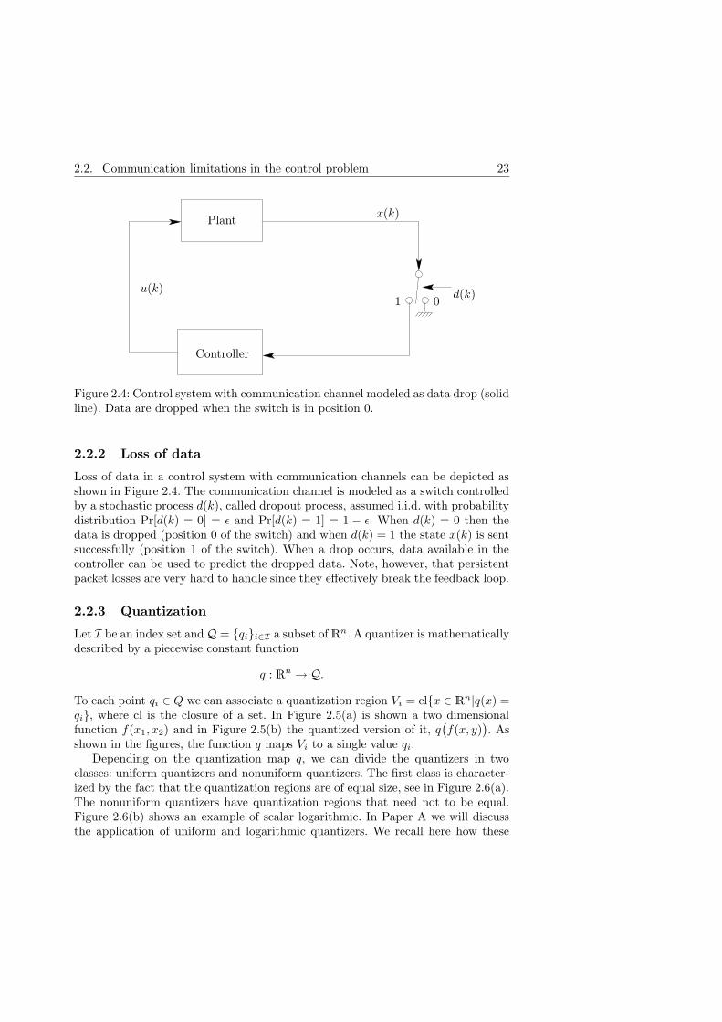
2.2.2 Loss of data
Loss of data in a control system with communication channels can be depicted asshown in Figure 2.4. The communication channel is modeled as a switch controlledby a stochastic process d(k), called dropout process, assumed i.i.d. with probabilitydistribution Pr[d(k) = 0] = ε and Pr[d(k) = 1] = 1 − ε. When d(k) = 0 then thedata is dropped (position 0 of the switch) and when d(k) = 1 the state x(k) is sentsuccessfully (position 1 of the switch). When a drop occurs, data available in thecontroller can be used to predict the dropped data. Note, however, that persistentpacket losses are very hard to handle since they effectively break the feedback loop.
2.2.3 Quantization
Let I be an index set andQ = qii∈I a subset of Rn. A quantizer is mathematicallydescribed by a piecewise constant function
q : Rn → Q.
To each point qi ∈ Q we can associate a quantization region Vi = clx ∈ Rn|q(x) =
qi, where cl is the closure of a set. In Figure 2.5(a) is shown a two dimensionalfunction f(x1, x2) and in Figure 2.5(b) the quantized version of it, q
(f(x, y)
). As
shown in the figures, the function q maps Vi to a single value qi.Depending on the quantization map q, we can divide the quantizers in two
classes: uniform quantizers and nonuniform quantizers. The first class is character-ized by the fact that the quantization regions are of equal size, see in Figure 2.6(a).The nonuniform quantizers have quantization regions that need not to be equal.Figure 2.6(b) shows an example of scalar logarithmic. In Paper A we will discussthe application of uniform and logarithmic quantizers. We recall here how these

24 Chapter 2. Control under communication constraints
−6−4
−20
24
6
−6−4
−20
24
6−100
−80
−60
−40
−20
0
20
40
60
80
100
x1x2
f(x1, x2)
Vi
(a) Function f(x1, x2).
−6−4
−20
24
6
−5
0
5
26
26.5
27
27.5
28
q(f(x1, x2)
)
x1x2
•qi
Vi
(b) Quantized function, q(f(x, y)).
Figure 2.5: A 2D quantizer. Vi represents a quantization region and qi is the quan-tized value associated to the quantization region Vi.
PSfrag replacements
R
Q
Vi
(a) Uniform quantizer. The scalar case.
PSfrag replacements
R
Q
Vi
(b) Logarithmic quantizer. The scalar case.
Figure 2.6: Two different types of quantizers: uniform and logarithmic.
maps are defined. Let δ > 0 be the quantization step. A scalar uniform quantizeris a map qu : R→ Q such that
qu(x) = δ⌊xδ
⌋.
The quantization regions for a scalar uniform quantizer are the intervals Vi =[−δ/2 + iδ, δ/2 + iδ], i = Z.
A logarithmic quantizer is a map q` : R→ Q such that
q`(x) = exp(qu(lnx)).
The quantization regions for a scalar logarithmic quantizer are the intervals Vi =[exp(−δ/2 + iδ), exp(δ/2 + iδ)], i = Z.
2.2. Communication limitations in the control problem 25
PSfrag replacements
Plant
Quantizer
Controller
x(k)
q(x(k)
)
u(k) = g(q(x(k))
)
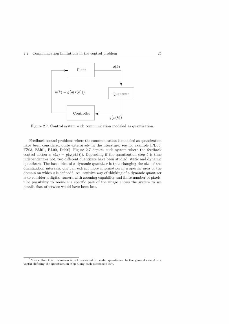
Figure 2.7: Control system with communication modeled as quantization.
Feedback control problems where the communication is modeled as quantizationhave been considered quite extensively in the literature, see for example [PB03,FZ03, EM01, BL00, Del90]. Figure 2.7 depicts such system where the feedbackcontrol action is u(k) = g(q(x(k))). Depending if the quantization step δ is timeindependent or not, two different quantizers have been studied: static and dynamicquantizers. The basic idea of a dynamic quantizer is that changing the size of thequantization intervals, one can extract more information in a specific area of thedomain on which q is defined5. An intuitive way of thinking of a dynamic quantizeris to consider a digital camera with zooming capability and finite number of pixels.The possibility to zoom-in a specific part of the image allows the system to seedetails that otherwise would have been lost.
5Notice that this discussion is not restricted to scalar quantizers. In the general case δ is avector defining the quantization step along each dimension Rn.


Chapter 3Autonomous multi-robot systems
“If you want to be incrementally better: Be competitive. If youwant to be exponentially better: Be cooperative.”
- Anonymous
A multi-robot system is a collection of robots which cooperate to solve a commontask. Such systems exhibit many advantages compared to single-robot solutions,such as flexibility, robustness, feasibility, efficiency [DGR00, Par00, KYC+96]. Thepossibility of splitting the robots in groups [SVS04] performing tasks at differentlocations, the ability of completing a task even if some robot breaks down [GC01],the capability of fusing sensor data in order to obtain better information about theenvironment [MSJH04], are few examples of the potential of multi-robot systemcompared to single-robot solutions. However, in order to design cooperative controlstrategies for multi-robot systems with such properties, a mathematical model ofthe system and the task is needed. In the following we present mathematical modelsof common mobile robot platform and then review some mathematical models formulti-robot systems that have some relationships with the models used in threepapers included in the thesis.
3.1 Single-robot models
We review here some common mathematical models of single robots.
3.1.1 Unicycle robot
A unicycle robot is composed of two independently actuated wheels and a smallpassive castor wheel used to keep the balance. The simplest kinematic model for
27

28 Chapter 3. Autonomous multi-robot systems
(a) Unicycle robot used by the Padova teamduring the Robocup world cup champi-onship in 1999. The platform is a modi-fied version of a Pioneer robot of ActivMe-dia. [PDF+03].
PSfrag replacements
(x, y)
Castor wheel
Fixed wheel
X
Y
θ
(z1, z2)
L
(b) The unicycle model.
Figure 3.1: Unicycle robot.
the unicycle is given by
x = v cos θ
y = v sin θ
θ = ω
where (x, y) is the center point of the front wheel axis and θ is the orientation ofthe unicycle, see Figure 3.1(b). All quantities are respect a global coordinate frame.The input signals v and ω are the translational and angular velocities, respectively.The unicycle model is used to describe many indoor robots, such as the robotshown in Figure 3.1(a) as well as outdoor mobile robots with skid-steer capabilities(caterpillar-like robots).
3.1. Single-robot models 29
PSfrag replacements
(x, y)
L
φ
X
Y θ
Figure 3.2: Car-like robot.
3.1.2 Car-like robot
A car-like robot is shown in Figure 3.2. The mathematical model is
x = v cos θ
y = v sin θ
θ =v tanφ
L.
The control inputs are the velocity v and the steering angle φ. The model is verysimilar to that of a unicycle. The main difference is that θ depends on v. Thus, fora car-like robot it is not possible to turn on place.
3.1.3 Underwater robot
Autonomous underwater vehicles (AUV’s) are typically small unmanned submarines.In Figure 3.3 is shown a photo of the AUV Isurus of University of Porto, Portugal.
Referring to Figure 3.4, we have
• (x, y, z)T is the position of the vehicle with respect to a global coordinatesystem,
• (φ, θ, ψ)T is the attitude of the vehicle with respect to a global coordinatesystem,
• (u, v, w)T are the linear velocities with respect to a body-fixed coordinateframe,
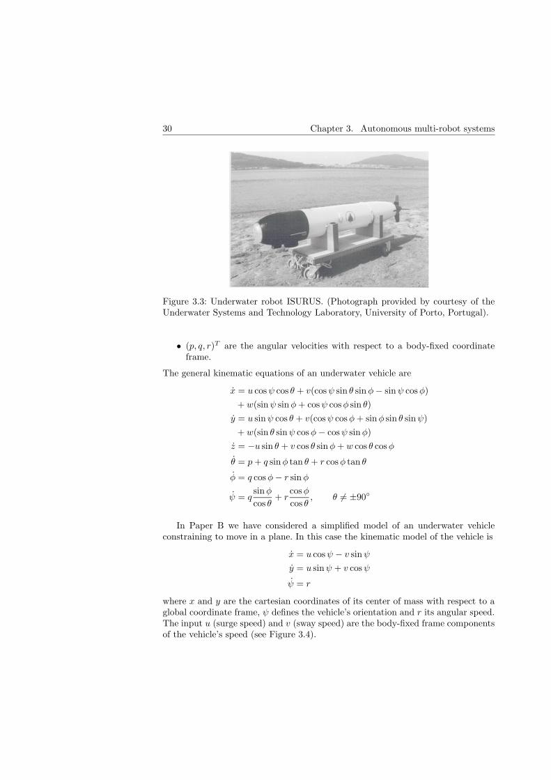
30 Chapter 3. Autonomous multi-robot systems
Figure 3.3: Underwater robot ISURUS. (Photograph provided by courtesy of theUnderwater Systems and Technology Laboratory, University of Porto, Portugal).
• (p, q, r)T are the angular velocities with respect to a body-fixed coordinateframe.
The general kinematic equations of an underwater vehicle are
x = u cosψ cos θ + v(cosψ sin θ sinφ− sinψ cosφ)
+ w(sinψ sinφ+ cosψ cosφ sin θ)
y = u sinψ cos θ + v(cosψ cosφ+ sinφ sin θ sinψ)
+ w(sin θ sinψ cosφ− cosψ sinφ)
z = −u sin θ + v cos θ sinφ+ w cos θ cosφ
θ = p+ q sinφ tan θ + r cosφ tan θ
φ = q cosφ− r sinφ
ψ = qsinφ
cos θ+ r
cosφ
cos θ, θ 6= ±90
In Paper B we have considered a simplified model of an underwater vehicleconstraining to move in a plane. In this case the kinematic model of the vehicle is
x = u cosψ − v sinψ
y = u sinψ + v cosψ
ψ = r
where x and y are the cartesian coordinates of its center of mass with respect to aglobal coordinate frame, ψ defines the vehicle’s orientation and r its angular speed.The input u (surge speed) and v (sway speed) are the body-fixed frame componentsof the vehicle’s speed (see Figure 3.4).

3.2. Multi-robots mathematical model 31
PSfrag replacements
xb
yb
zb
X
Y
Z
u (surge)
p (roll)w (heave)
r (yaw)
v (sway)q (pitch)
(x, y, z)
Figure 3.4: Underwater robot.
3.2 Multi-robots mathematical model
In the previous sections, we have described typical mathematical models for single-robot systems. For multi-robot systems several mathematical models have beenproposed in the literature. We will review here some of these models that haveimportant connections with those proposed in the papers included in this thesis.
3.2.1 Formation graph
The idea of associating a graph to a team of robots to model the interactionsamong robots is quite natural. In such model, each robot of the system can beviewed as a vertex of a graph G = (V, E). An edge exists between two vertices ifthe robots associated to those vertexes interact in some way. Algebraic propertiesof the matrices associated to the graph G can be used to analyze the properties ofthe overall multi-robot system. In particular, in Paper A, we associated to a multi-robot system a graph which represents the local interaction between the robots,and specifically an exchange of information. Examples, in the literature, includedeployment and coverage tasks as in [CMB04], or the problem of organizing therobots in formations as in [OSM02].
3.2.2 Hierarchical structure
A hierarchical control structure can be used to model multi-robot systems [DLS95].Each robot is described by three different layers: an upper layer which is modeledby a discrete-event system, a lower layer which is represented by a continuous-timesystem and an interface which interconnects the two layers, as shown in Figure 3.5.The upper layer, which we call here team controller, is responsible for generating
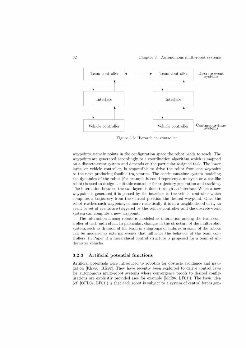
32 Chapter 3. Autonomous multi-robot systems
PSfrag replacements
Team controllerTeam controller
Vehicle controller Vehicle controller
InterfaceInterface
Discrete-eventsystems
Continuous-timesystems
Figure 3.5: Hierarchical controller
waypoints, namely points in the configuration space the robot needs to reach. Thewaypoints are generated accordingly to a coordination algorithm which is mappedon a discrete-event system and depends on the particular assigned task. The lowerlayer, or vehicle controller, is responsible to drive the robot from one waypointto the next producing feasible trajectories. The continuous-time system modelingthe dynamics of the robot (for example it could represent a unicycle or a car-likerobot) is used to design a suitable controller for trajectory generation and tracking.The interaction between the two layers is done through an interface. When a newwaypoint is generated it is passed by the interface to the vehicle controller whichcomputes a trajectory from the current position the desired waypoint. Once therobot reaches such waypoint, or more realistically it is in a neighborhood of it, anevent or set of events are triggered by the vehicle controller and the discrete-eventsystem can compute a new waypoint.
The interaction among robots is modeled as interaction among the team con-troller of each individual. In particular, changes in the structure of the multi-robotsystem, such as division of the team in subgroups or failures in some of the robotscan be modeled as external events that influence the behavior of the team con-trollers. In Paper B a hierarchical control structure is proposed for a team of un-derwater vehicles.
3.2.3 Artificial potential functions
Artificial potentials were introduced to robotics for obstacle avoidance and navi-gation [Kha86, RK92]. They have recently been exploited to derive control lawsfor autonomous multi-robot systems where convergence proofs to desired config-urations are explicitly provided (see for example [McI96, LF01]). The basic idea(cf. [OFL04, LF01]) is that each robot is subject to a system of central forces gen-
3.2. Multi-robots mathematical model 33
erated by artificial potential fields. In particular there are inter-robot forces that arenegative when the relative distance between two robots is less than a fixed thresh-old and vanishe when the robots are far from each other. Robots are also subjectto forces directed towards some other robots which represent virtual leaders of thegroup. A controlled dissipative force is also applied to each robot and is designedsuch that it is zero when the robot is moving at the desired speed. Thus a teamof robot embedded in such artificial potential fields can be analyzed as a system ofvirtual forces and a controller is designed based on the inter-robot forces.
In Paper C a probabilistic pursuit–evasion game is considered. Each pursuerscreate probabilistic maps, which can be considered as an artificial potential field,in order to move in an unknown environment.


Chapter 4Multi-robot systems with
communication constraints
“The most important thing in communication is to hear what isn’tbeing said.”
- P.F. Drucker
A multi-robot system with communication constraints is a special case of distributedcontrol system with subsystems interconnected with digital communication chan-nels. A block diagram showing three robots connected via communication links isshown Figure 4.1. A particular restriction, compared with the general distributedsystem discussed in previous chapters (see Figure 2.1) is that only controllers ex-change data.
The design of controllers for multi-robot systems has been mostly focused onthe development of cooperative strategies, where a team of robots accomplish agiven task [LF01, FBKT00, HKS99, BA98]. Communication, when present, hasbeen considered as a system property and limitations have seldom been accountedfor in the design. As the applications grow in complexity the limitations becomemore important; for example, when the number of robots is large or when therobots are deployed in particular environments, such as underwater or in space.A general theory for control design of multi-robot systems under communicationconstraints is not existing and few results are available in the literature. We willpresent here two interesting frameworks for modeling these type of problems whentopological communication constraints are considered, namely constraints on “whocan communicate with who”.
35

36 Chapter 4. Multi-robot systems with communication constraints
PSfrag replacements
Actuator Actuator
Actuator
Sensor Sensor
Sensor
Controller Controller
Controller
T/R T/R
T/R
Robot 1 Robot 2
Robot 3
Figure 4.1: Multi-robot system with communication channels depicted. The solidarrows represent wireless communication channels and empty arrows represent thesensor and actuation signals. The T/R blocks represent the transmitters and re-ceivers of the digital communication systems.
4.1 Team decision theory
The problem of designing control strategies for a team of robots when communi-cation constraints are topological can be related to the problem studied in teamdecision theory [Chu72, HC72, Wit68]. We summarize here the model and someimportant results developed.
Let us consider a team of n robots. There are five basic ingredients of decisiontheory.
1. The state of the world ξ = (ξ1, . . . , ξn) ∈ Ω is capture by a vector of randomvariables defined on a suitable probability space. The vector ξ represents allthe uncertainties in the problem under consideration, e.g. unknown initialconditions, measurement noise, uncertain parameters, etc.
2. A set of decision variables u = (u1, . . . , un) ∈ U , each representing the decision

4.1. Team decision theory 37
of one robot.
3. A measurable function J(ξ, u), called payoff function.
4. A set of information functions z = η(ξ, u) ∈ Z, so that z = (η1(ξ, u), . . . , ηn(ξ, u).In other words zi represents the information known to the robot i. This in-cludes information communicated by other robots. The set η1, . . . , ηn isknown as the information structure.
5. A set of strategies γ = (γ1, . . . , γn) ∈ Γ, where γi is a mapping from thezi-space to the ui-space. Robot i must choose actions ui = γi(zi) based onhis local information, hence the problem is decentralized.
The dynamic team decision problem is
minγ∈Γ
E[J(ξ, γ(η(ξ, u)))
].
The reason why the problem is called dynamic is because z = η(ξ, u). If z = η(ξ)the problem is said to be static. In the simplest case the information functions arelinear in ξ and in the control actions other member have taken, namely
zi = Hiξ +∑
j
Di,juj , ∀i ∈ I.
where Hi and Di,j are matrices of appropriate dimensions and are known to eachrobot. The information structure in this case is defined as the matrices Hi and Di,j ,with i, j ∈ I. Roughly speaking the information structure is a formal notion of “whoknows what”. Notice that no dynamics in the topology is allowed i.e., Hi and Di,j
are not time dependent.
Since we interested in modeling causal systems, we assume
Di,j 6= 0⇒ Dj,i = 0 ∀i, j ∈ I, i 6= j.
Thus if the control action of j affects the information of i, then the control actionof i cannot affect the information of j i.e., we have in mind here a discrete-timedynamic situation in which the current actions can affect, at most, information inthe succeeding, but not current, stage. This means that we can graphically representthe information structure by a precedence diagram. Let us consider an example.
Example 4.1Consider the multi-robot system of Figure 4.2a. The information structure can berepresented by the precedence diagram of Figure 4.2b, showing how the informationof each robot influences the information of the others. The information is then given
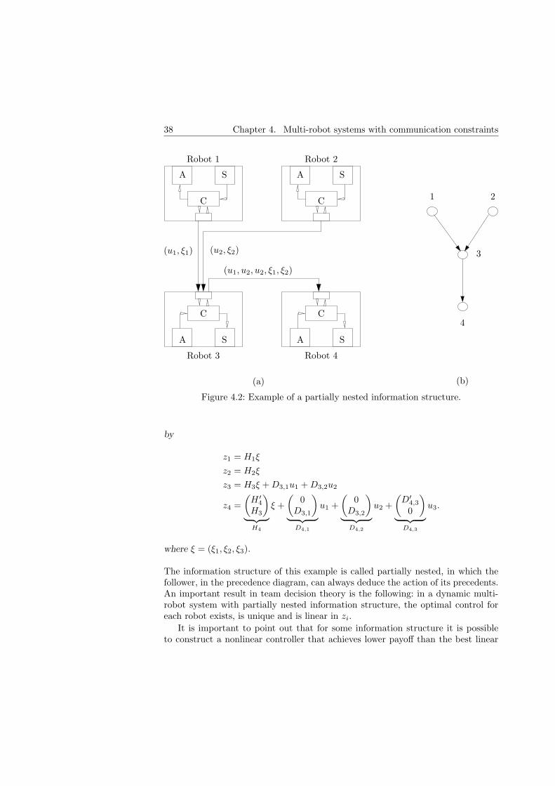
38 Chapter 4. Multi-robot systems with communication constraints
PSfrag replacements 1 2
3
4
Robot 1 Robot 2
Robot 3 Robot 4
CC
CC
AA
AA
SS
SS
(a) (b)
(u1, ξ1) (u2, ξ2)
(u1, u2, u2, ξ1, ξ2)
Figure 4.2: Example of a partially nested information structure.
by
z1 = H1ξ
z2 = H2ξ
z3 = H3ξ +D3,1u1 +D3,2u2
z4 =
(H ′
4
H3
)
︸ ︷︷ ︸H4
ξ +
(0
D3,1
)
︸ ︷︷ ︸D4,1
u1 +
(0
D3,2
)
︸ ︷︷ ︸D4,2
u2 +
(D′
4,3
0
)
︸ ︷︷ ︸D4,3
u3.
where ξ = (ξ1, ξ2, ξ3).
The information structure of this example is called partially nested, in which thefollower, in the precedence diagram, can always deduce the action of its precedents.An important result in team decision theory is the following: in a dynamic multi-robot system with partially nested information structure, the optimal control foreach robot exists, is unique and is linear in zi.
It is important to point out that for some information structure it is possibleto construct a nonlinear controller that achieves lower payoff than the best linear
4.2. Consensus problems 39
PSfrag replacements
(a) (b) (c)
Figure 4.3: Example of n = 11 robots in a formation control problem. The headingof the formation is the average of the single robot heading.
one (see [Wit68]). Thus only for specific communication topologies it is possible tocompute the control strategies that optimize the payoff.
4.2 Consensus problems
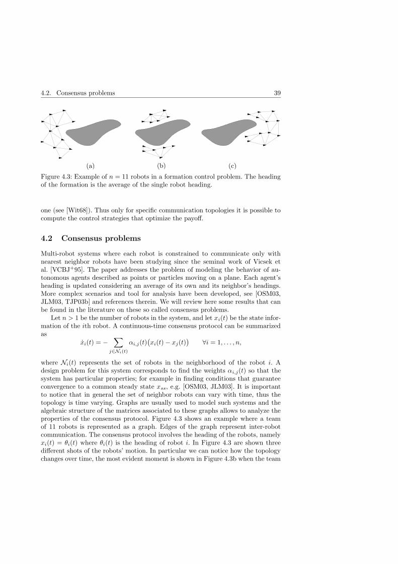
Multi-robot systems where each robot is constrained to communicate only withnearest neighbor robots have been studying since the seminal work of Vicsek etal. [VCBJ+95]. The paper addresses the problem of modeling the behavior of au-tonomous agents described as points or particles moving on a plane. Each agent’sheading is updated considering an average of its own and its neighbor’s headings.More complex scenarios and tool for analysis have been developed, see [OSM03,JLM03, TJP03b] and references therein. We will review here some results that canbe found in the literature on these so called consensus problems.
Let n > 1 be the number of robots in the system, and let xi(t) be the state infor-mation of the ith robot. A continuous-time consensus protocol can be summarizedas
xi(t) = −∑
j∈Ni(t)
αi,j(t)(xi(t)− xj(t)
)∀i = 1, . . . , n,
where Ni(t) represents the set of robots in the neighborhood of the robot i. Adesign problem for this system corresponds to find the weights αi,j(t) so that thesystem has particular properties; for example in finding conditions that guaranteeconvergence to a common steady state xss, e.g. [OSM03, JLM03]. It is importantto notice that in general the set of neighbor robots can vary with time, thus thetopology is time varying. Graphs are usually used to model such systems and thealgebraic structure of the matrices associated to these graphs allows to analyze theproperties of the consensus protocol. Figure 4.3 shows an example where a teamof 11 robots is represented as a graph. Edges of the graph represent inter-robotcommunication. The consensus protocol involves the heading of the robots, namelyxi(t) = θi(t) where θi(t) is the heading of robot i. In Figure 4.3 are shown threedifferent shots of the robots’ motion. In particular we can notice how the topologychanges over time, the most evident moment is shown in Figure 4.3b when the team

40 Chapter 4. Multi-robot systems with communication constraints
splits in two independent groups to avoid an obstacle (shown in gray). Figure 4.3cshows the robots forming again a single group and heading in the same direction.
Let Gpp∈P be all the possible graphs with n vertices, parameterized by theindex p ∈ P with P a suitable index set. Let σ : 1, 2, . . . → P denote a switchingsignal. Then it is possible to prove that the consensus is achieved, namely
limt→∞
θi(t) = θss ∀i = 1, . . . , n,
if the graphs Gσ(t) are connected most of the time [JLM03]. Moreover in [Jad03]it is proved that a necessary and sufficient condition for the robots to convergeto a steady state is that the switching of topologies converges in finite time to aconnected topology, and no more switches occur. Namely ∃T > 0 such that
Gσ(T ) = GM , M ∈ P
with GM connected and σ(t) = M for all t > T . The main limitation of theseresults, at this point of the development, is the lack of general existence conditionsi.e., given a consensus problem we do not know if there exists a time T > 0 suchthat the topologies will be connected or if the topologies are connected most of thetime.
Consensus problem have been used in literature to solve different types of prob-lems, e.g. formation [GHM03, FM02], rendezvous [LMA03] and flocking [TJP03a,TJP03b] problems.
4.3 Towards a theory for multi-robot systems
The development of systematic methods for the analysis and design of controllersfor multi-robot systems under communication constraint has become a very impor-tant research area since applications have become more demanding, both from thecomplexity of the tasks that have to be solve and the amount of data exchangedby the robots. Team decision theory and consensus problems are two possible ap-proaches for studying multi-robot systems under communication constraints. How-ever, the limitations imposed by the communication system, in both approaches,are restricted to topological constraints. In Chapter 2 we have listed other impor-tant limitations the communication channel imposes such as time delays, loss ofdata and quantization. Towards the development of general tools for multi-robotsystems, in the papers included in the thesis we have studied the effects of some ofthese limitations to specific multi-robot tasks.
References
[BA98] T. Balch and R C. Arkin. Behavior-based formation control for multi-robot teams. IEEE Transaction on Robotics and Automation, 14:926–939, 1998.
[BL00] R.W. Brockett and D. Liberzon. Quantized feedback stabilization oflinear systems. IEEE Transaction on Automatic Control, 45(7):1279–1289, 2000.
[Chu72] K.C. Chu. Team decision theory and information structures in optimalcontrol problems - part 2. IEEE Transaction on Automatic Control,17(17):22–28, February 1972.
[CMB04] J. Cortes, S. Martinez, and F. Bullo. Spatially-distributed coverage op-timization and control with limited-range interactions. ESAIM: Con-trol, Optimisation, and Calculus of Variations, 2004. Submitted.
[CT91] T.M. Cover and J.A. Thomas. Elements of information theory. WileyInterscience, 1991.
[Del90] D.F. Delchamps. Stabilizing a liner system with quantized state feed-back. IEEE Transaction on Automatic Control, 35:916–924, 1990.
[DGR00] B.R. Donald, L. Gariepy, and D. Rus. Distributed manipulation ofmultiple objects using ropes. In IEEE International Conference onRobotics and Automation, pages 450–457, 2000.
[DLS95] N.G. Datta, J. Lygeros, and S. Sastry. Hierarchical hybrid control:a case study”, pages 166–190. Lecture Notes in Computer Science,Springer, 1995.
[EM01] N. Elia and S. J. Mitter. Stabilization of linear systems with limitedinformation. IEEE Transaction on Automatic and Control, 46(9):1384–1400, 2001.
41
42 References
[FBKT00] D. Fox, W. Burgard, H. Kruppa, and S. Thrun. A probabilistic ap-proach to collaborative multi-robot localization. Special issue of Au-tonomous Robots on Heterogeneous Multi-Robot Systems, 3, 2000.
[FM02] J.A. Fax and R.M. Murray. Information flow and cooperative controlof vehicles formations. In IFAC World Congress, 2002.
[FZ03] F. Fagnani and S. Zampieri. Stability analysis and synthesis for scalarlinear systems with quantized feedback. IEEE Transaction on Auto-matic and Control, 48(9):1569–1584, 2003.
[GC01] K. Goldberg and B. Chen. Collaborative control of robot motion: Ro-bustness to error. In IEEE/RSJ International Conference on Robotsand Systems, 2001.
[GHM03] V. Gupta, B. Hassibi, and R. Murray. Stability analysis of stochasticvarying formation of dynamic agents. In IEEE Conference on Decisionand Control, 2003.
[HC72] Y. Ho and K.C. Chu. Team decision theory and information structuresin optimal control problems - part 1. IEEE Transaction on AutomaticControl, 17(1):15–22, February 1972.
[HKS99] J.P. Hespanha, H. J. Kim, and S. Sastry. Multiple-agent probabilisticpursuit–evasion games. In IEEE Conference on Decision and Control,volume 3, pages 2432–2437, 1999.
[Jad03] A. Jadbabaie. On coordination strategies for mobile agents with chang-ing nearest neighbor sets. In IEEE Mediterranian Conference on Con-trol and Automation, 2003.
[JLM03] A. Jadbabaie, J. Lin, and A.S. Morse. Coordination of groups of mobileautonomous agents using nearest neighbor rules. IEEE Transactionson Automatic Control, 48(6):988–1001, 2003.
[Kha86] O. Khatib. Real time obstacle avoidance for manipulators and mobilerobots. International Journal of Robotics Research, 5:90–99, 1986.
[KYC+96] O. Khatib, K. Yokoi, K. Chang, R. Holmberg, and A. Casal. Vehi-cle/arm coordination and mobile manipulator decentralized coopera-tion. In IEEE/RSJ International Conference on Intelligent Robots andSystems, pages 546–553, 1996.
[LF01] N.E. Leonard and E. Fiorelli. Virtual leaders, artificial potentials andcoordinated control of groups. In IEEE Conference on Decision andControl, pages 2968–2973, 2001.

43
[LMA03] J. Lin, A. S. Morse, and B. D. O. Anderson. The multi-agent ren-dezvous problem. In Proc. of the 42nd IEEE Conference on Decisionand Control, HI, USA, 2003.
[McI96] C.R. McInnes. Potential function methods for autonomous spacecraftguidance and control. Advances in Astronautical Sciences, pages 2093–2109, 1996.
[Mit01] S.J. Mitter. Control with limited information. European Journal ofControl, 7(1), 2001.
[MSJH04] M. Mazo, A. Speranzon, K.H. Johansson, and X. Hu. Multi-robottracking of a moving object using directional sensors. In IEEE Inter-national Conference on Robotics and Automation, 2004.
[Nil98] J. Nilsson. Real-time control systems with delays. PhD thesis, LundInstitute of Technology, 1998.
[OFL04] P. Ogren, E. Fiorelli, and N.E. Leonard. Cooperative control of mobilesensor networks: Adaptive gradient climbing in a distributed environ-ment. IEEE Transaction on Automatic and Control, 2004.
[OSM02] R. Olfati-Saber and R.M. Murray. Graph rigidity and distributed for-mation stabilization of multi-vehicle systems. In IEEE Conference onDecision and Control, 2002.
[OSM03] R. Olfati Saber and M. Murray. Flocking with obstacle avoidance:cooperation with limited communication in mobile networks. In IEEEConference on Decision and Control, 2003.
[Par00] L. Parker. Current state of the art in distributed robot systems.In Berhen J. Parker L., Bekey G., editor, Distributed AutonomousRobotics Systems 4. Springer, 2000.
[PB03] B. Picasso and A. Bicchi. Stabilization of LTI systems with quantizedstate-quantized input static feedback. In A. Pnueli and O. Maler, ed-itors, Hybrid Systems: Computation and Control, volume LNCS 2623of Lecture Notes in Computer Science. Springer-Verlag, 2003.
[PDF+03] E. Pagello, A. D’Angelo, C. Ferrari, R. Polesel, R. Rosati, and A. Sper-anzon. Emergent behaviors of a robot team performing cooperativetasks. Advanced Robotics, 15(1):3–20, 2003.
[RK92] E. Rimon and D.E. Koditschek. Exact robot navigation using artificialpotential functions. IEEE Transactions on Robotics and Automation,8:501–508, 1992.

44 References
[Sha48] C.E. Shannon. A mathematical theory of communication. Bell SystemTechnical Journal, 27:379–423,623–656, 1948.
[SVS04] J. Sousa, P. Varaiya, and T. Simsek. Distributed control of teamsof unmanned air vehicles. In Mathematical Theory of Networks andSystems, 2004.
[TJP03a] H.G. Tanner, A. Jadbabaie, and G.J. Pappas. Stable flocking of mobileagents, part i: fixed topology. In IEEE Conference on decision andcontrol, 2003.
[TJP03b] H.G. Tanner, A. Jadbabaie, and G.J. Pappas. Stable flocking of mobileagents, part ii: dynamic topology. In IEEE Conference on decision andcontrol, 2003.
[VCBJ+95] T Vicsek, A. Czirok, Eshel Ben-Jaco, I. Cohen, and O. Shochet. Noveltype of phase transition in a system of self-driven particles. PhysicalReview Letters, 75:1226–1229, 1995.
[Wit68] H.S. Witsenhausen. A counterexample in stochastic optimum control.SIAM Journal of Control, 6(1):131–147, 1968.
[XHH00] L. Xiao, A. Hassibi, and J.P. How. Control with random communi-cation delays via a discrete-time jump system approach. In AmericanControl Conference, 2000.

Part II
Papers
45

Paper A
On Multi-Vehicle Rendezvous
Under Quantized Communication
F. Fagnani, K.H. Johansson, A. Speranzon, S. Zampieri
Abstract
A rendezvous problem for a team of autonomous vehicles, which communicate overquantized channels, is analyzed. The paper illustrates how communication topolo-gies based on uniform and logarithmic quantization influence the performance. Sincea logarithmic quantizer in general imposes fewer bits to be communicated comparedto a uniform quantizer, the results indicate estimates of lower limits on the amountof information that needs to be exchanged in order for the vehicles to meet. Simu-lation examples illustrate the results.
Keyworkds: Quantized communication, Rendezvous, Multi-vehicle system.
5.1. Introduction 49
5.1 Introduction
Interplay between coordination and communication is important in many multi-vehicle systems, e.g., car platoons on automated highways [Var93], formations ofautonomous underwater vehicles [dSP02], and multi-robot search-and-rescue mis-sions[SJ03]. Constrained communication between vehicles suggest the deployment ofdistributed (local) control strategies [LMA03, SM03]. In many cases not only thecommunication topology is important, however, but also the amount of data beingtransmitted. Therefore, in this paper we study multi-vehicle control under quan-tized communication. The problem is related to the stabilization of linear plantswith quantized control, which has recently been extensively studied, see [FZ03] andreferences therein.
The main contribution of this paper is to illustrates how communication topolo-gies based on uniformly and logarithmically quantized communication influencethe solution to a multi-vehicle rendezvous problem. A team of autonomous vehicleswith only local position information is to meet under minimum communication ca-pabilities. We prove the existence of several classes of solutions to this rendezvousproblem. In particular, we emphasize that uniform quantizers can sometimes bereplaced by logarithmic quantizers and thus reduce the need for communicationbandwidth.
The outline of the paper is as follows. The rendezvous problem is defined inSection 5.2 together with feasible communication topologies. A few illustrative two-vehicle cases are studied in detail in Section 5.3. Teams of three and more vehiclesare then considered in Section 5.4. Convergence properties are investigated throughsimulations in Section 5.5. Some conclusions are given in Section 5.6.
5.2 Problem formulation
Consider n > 2 vehicles moving in a plane, with dynamics described by the discrete-time system
x+ = x + u (5.1)
y+ = y + v (5.2)
where x = (x1, . . . , xn)T ∈ X ⊂ Rn and y = (y1, . . . , yn)T ∈ Y ⊂ R
n, so that(xi, yi) denotes the position of vehicle i with respect to a fixed coordinate system.Let U ⊂ R
n and V ⊂ Rn denote the set of control values. The controls u =
(u1, . . . , un) and v = (v1, . . . , vn) we are considering are feedback maps from thecorresponding state-space X and Y, respectively. Since the control of the x- andy-coordinates are independent, we only consider x in the sequel.
50
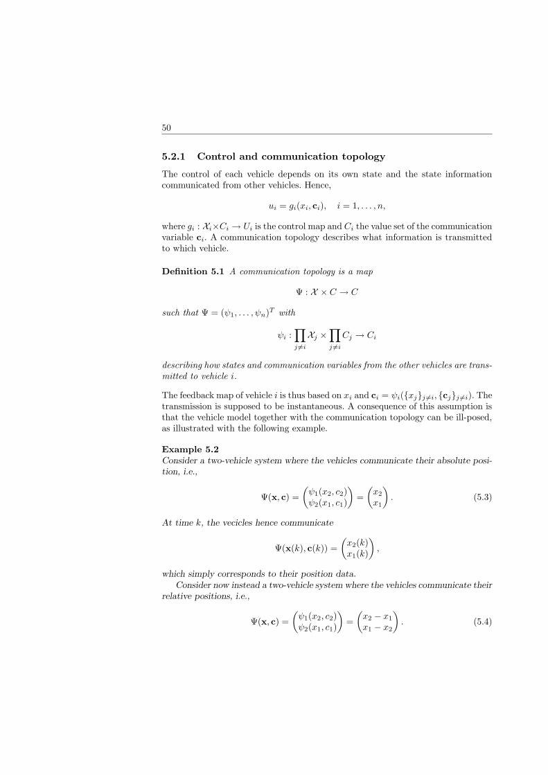
5.2.1 Control and communication topology
The control of each vehicle depends on its own state and the state informationcommunicated from other vehicles. Hence,
ui = gi(xi, ci), i = 1, . . . , n,
where gi : Xi×Ci → Ui is the control map and Ci the value set of the communicationvariable ci. A communication topology describes what information is transmittedto which vehicle.
Definition 5.1 A communication topology is a map
Ψ : X × C → C
such that Ψ = (ψ1, . . . , ψn)T with
ψi :∏
j 6=i
Xj ×∏
j 6=i
Cj → Ci
describing how states and communication variables from the other vehicles are trans-mitted to vehicle i.
The feedback map of vehicle i is thus based on xi and ci = ψi(xjj 6=i, cjj 6=i). Thetransmission is supposed to be instantaneous. A consequence of this assumption isthat the vehicle model together with the communication topology can be ill-posed,as illustrated with the following example.
Example 5.2Consider a two-vehicle system where the vehicles communicate their absolute posi-tion, i.e.,
Ψ(x, c) =
(ψ1(x2, c2)ψ2(x1, c1)
)=
(x2
x1
). (5.3)
At time k, the vecicles hence communicate
Ψ(x(k), c(k)) =
(x2(k)x1(k)
),
which simply corresponds to their position data.Consider now instead a two-vehicle system where the vehicles communicate their
relative positions, i.e.,
Ψ(x, c) =
(ψ1(x2, c2)ψ2(x1, c1)
)=
(x2 − x1
x1 − x2
). (5.4)
5.2. Problem formulation 51
At time k, the vehicles should then communicate
Ψ(x(k), c(k)) =
(x2(k)− x1(k)x1(k)− x2(k)
),
which is not possible. This fact can be easily seen from that at time k = 0, eachvehicle know only their initial position x1(0) = x10 and x2(0) = x20, respectively,so its impossible to communicate the differences
Ψ(x(0), c(0)) =
(x2(0)− x1(0)x1(0)− x2(0)
).
Hence, the communication topology with relative positions is not feasible in thesense that it cannot be realized.
We consider only topologies that are physically realizable, i.e., feasible communica-tion topologies according to the following definition.
Definition 5.2 A communication topology is feasible if there exists a surjectivemap f : X → C such that
c = Ψ(x, c) ⇒ c = f(x).
The notion of feasibility for a communication topology given here is related tothe concept of deadlock-freeness introduced in [AT92] for decentralized stochasticsystems.
Example 2 (cont’d). It easy to see that (5.3) yields a feasible communicationtopology, while (5.4) is unfeasible.
5.2.2 Quantized communication
We further restrict the communication by imposing that communicated data arequantized. In particular, uniform and logarithmic quantizations are considered. Re-call the following definitions of scalar uniform and logarithmic quantizers.
Definition 5.3 Let δ be a positive parameter. A uniform quantizer is a map qu :R→ R such that
qu(x) = δ⌊xδ
⌋.
Notice that the error due to the quantization of a variable x is bounded by δ i.e.,
|qu(x)− x| 6 δ. (5.5)
Definition 5.4 Let δ be a positive parameter. A logarithmic quantizer is a mapq` : R→ R such that
q`(x) = exp(qu(lnx)).
52
The quantization error for a logarithmic quantizer is bounded as
|ql(x)− x| 6 δ|x|. (5.6)
We are interested in how communication topology and quantization of trans-mitted data influence the performance of the multi-vehicle system. Therefore, weconsider classes of maps Ψδ composed of various configurations of uniform and loga-rithmic quantizers. For simplicity, we suppose that all quantizers are parameterizedin a single quantization parameter δ.
Example 5.3For a two-vehicle system, a uniformly quantized communication topology is givenby
Ψδ(x, c) =
(ψ1(x2, c2)ψ2(x1, c1)
)=
(qu(x2)qu(x1)
).
5.2.3 Rendezvous
We are interested in the convergence to a multi-vehicle formation under quantizedcommunication topology. Especially, we pose the following rendezvous problem.
Definition 5.5 A feedback map g = (g1, . . . , gn) and a communication topology Ψδ
solve the rendezvous problem if for all initial states x0 ∈ X , and for all ε > 0, thereexists δ = δ(ε) such that
xi − xj → Bε
with i < j and i, j = 1, . . . , n.
A solution to the rendezvous problem is able to make the vehicles converge arbi-trarily close to a meeting point. Note that the meeting point is not pre-specified,but is only restricted to be close to the hyperplane x1 = · · · = xn.
If the communication is not quantized, then the rendezvous problem is readilysolved also in the case with no communication, i.e., when Ψ is empty. In this case, adecentralized deadbeat controller provides a solution. We consider such a solutiontrivial, since it enforces the vehicles to meet in the origin. It is instead desirable tohave the meeting point close to the initial position of the vehicles. In next section, wepresent a linear quadratic control problem for the two-vehicle system that addressthis problem and that also suggest a natural extension to the quantized case.
5.3 Two-vehicles rendezvous
Let the communication topology of a two-vehicle system be
Ψ0(x, c) =
(ψ1(x1, c1)ψ1(x2, c2)
)=
(x1
x2
).
5.3. Two-vehicles rendezvous 53
Let z = x1 − x2 be the output of the system (5.1) when n = 2. In order to avoidaggressive solution such as the dead-beat control we need to penalize the controlinput. Thus we consider an LQ problem with cost
J(u1, u2) =∞∑
t=0
z2 + u21 + u2
2
=
∞∑
t=0
(x1 + x2)2 + u2
1 + u22.
The resulting state feedback u = Kx gives the closed-loop system
x+1 = x1 − k(x1 − x2)
x+2 = x2 − k(x2 − x1), (5.7)
with k = 1/(1 +√
3). It corresponds to
z+ = (1− 2k)z,
which is asymptotically stable, meaning that the difference x1 − x2 tends to zeroasymptotically. Note that (5.7) it is not asymptotically stabile. The two vehicles,in general, will thus rendezvous at a point different from the origin.
The linear feedback K computed above is used to design controllers when thecommunication topology is composed of various configurations of uniform and log-arithmic quantizers.
5.3.1 Uniform-uniform quantization
Proposition 5.1 The feasible communication topology
Ψδ =
(ψ1(x2, c2)ψ2(x1, c1)
)=
(qu(x2)qu(x1)
)(5.8)
and the feedback
u1 = g1(x1, c1) = −k(x1 − c1)u2 = g2(x2, c2) = −k(x2 − c2) (5.9)
solve the rendezvous problem
Proof. Let us consider the difference z = x1 − x2. We introduce the followingLyapunov function V(z) = |z|. Thus the increment ∆V(z) = V(z+) − V(z) =|z+| − |z| is such that
∆V(z) = |z − 2kz − c1 + c2| − |z|6 −2k|z|+ 2kδ
54
where we have substituted c1 = ψ1 and c2 = ψ2 given in (5.8) and used (5.5). Hence∆V(z) < 0 if |z| > δ. If we choose δ = ε, then z will asymptotically converge to Bε.Thus the communication topology (5.8) and feedback (5.9) solves the rendezvousproblem.
Notice that instead of posing a deterministic LQ problem, we can consider astochastic LQ problem where the quantization error of the uniform quantizer isapproximated by additive white noise, namely
qu(x) = x+ e
and where e is white noise uniformly distributed in [−δ, δ] and Ee2 = δ2/12. Thisapproach yields the same feedback control as above.
5.3.2 Uniform-logarithmic quantization
Proposition 5.2 The feasible communication topology
Ψδ =
(ψ1(x2, c2)ψ2(x1, c1)
)=
(q`(qu(x1)− x2)
qu(x1)
)(5.10)
and the feedback
u1 = g1(x1, c1) = −k c1u2 = g2(x2, c2) = −k(x2 − c2) (5.11)
solve the rendezvous problem
Proof. Let us consider the difference z = x1−x2. As in the proof of Proposition 5.1,
∆V(z) = |z − k(c1 − x2 + c2)| − |z|6 −2k|z|+ k|z|δ + 2kδ + kδ2
where c1 and c2 are given by the communication topology map Ψδ defined in (5.10)and where we used (5.6). ∆V(z) < 0 if
|z| > 2δ(1 + δ)
2− δ .
If we choose δ = −1/2− ε/4−√
4 + 20ε+ ε2/4, z converges asymptotically to Bε.Thus the communication topology (5.10) and feedback (5.11) solves the rendezvousproblem.
The effect of the logarithmic quantization can be approximate as multiplicativenoise acting on the system. If, for simplicity, we neglect the presence of uniformquantization, then we have
x+1 = x1 + k11(x1 − x2)(1 + e)
x+2 = x2 + k22(x2 − x1)

5.3. Two-vehicles rendezvous 55
0 2 4 6 8 100
0.05
0.1
0.15
0.2
0.25
0.3
0.35
0.4k1(δ)
δ(a) k1(δ) as function of δ
0 2 4 6 8 100.3
0.35
0.4
0.45
0.5
0.55
0.6k2(δ)
δ(b) k2(δ) as function of δ
Figure 5.4: For large quantization step δ the value of k1(δ) tends to zero.
where e is white noise uniformly distributed in [−δ, δ] and variance Ee2(t) = δ2/12.Let z = x1 − x2, we consider an optimal control problem with cost
J(u1, u2) = E∞∑
t=0
z2 + u21(1 + e) + u2
2
= E∞∑
t=0
z2 + (u1, u2)
(1 + δ2
12 00 1
)
︸ ︷︷ ︸R
(u1
u2
)
and dynamics
z+ = z + (11)︸︷︷︸B
(u1
u2
)+ u1e.
The feedback law is linear and given by
K = (R+BTPB + Ω(P ))−1BTP
where P is the solution of a generalized Riccati difference equation and Ω(P ) is thefollowing matrix
Ω(P ) =
(1 + δ2
12 00 0
),
see [BD98]. The optimal feedback is
k1(δ) = k + aδ2 +O(δ4)
k2(δ) = k + bδ2 +O(δ4)
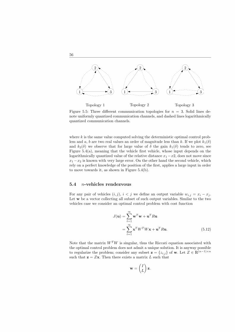
56
PSfrag replacements
1 11
2 22
33 3
c1c2c3
Topology 1 Topology 2 Topology 3
Figure 5.5: Three different communication topologies for n = 3. Solid lines de-note uniformly quantized communication channels, and dashed lines logarithmicallyquantized communication channels.
where k is the same value computed solving the deterministic optimal control prob-lem and a, b are two real values an order of magnitude less than k. If we plot k1(δ)and k2(δ) we observe that for large value of δ the gain k1(δ) tends to zero, seeFigure 5.4(a), meaning that the vehicle first vehicle, whose input depends on thelogarithmically quantized value of the relative distance x1−x2, does not move sincex1−x2 is known with very large error. On the other hand the second vehicle, whichrely on a perfect knowledge of the position of the first, applies a large input in orderto move towards it, as shown in Figure 5.4(b).
5.4 n-vehicles rendezvous
For any pair of vehicles (i, j), i < j we define an output variable wi,j = xi − xj .Let w be a vector collecting all subset of such output variables. Similar to the twovehicles case we consider an optimal control problem with cost function
J(u) =
∞∑
t=1
wT w + uTRu
=
∞∑
t=1
xTWTWx + uTRu. (5.12)
Note that the matrix W TW is singular, thus the Riccati equation associated withthe optimal control problem does not admit a unique solution. It is anyway possibleto regularize the problem; consider any subset z = zi,j of w. Let Z ∈ R
(n−1)×n
such that z = Zx. Then there exists a matrix L such that
w =
(IL
)z.

5.4. n-vehicles rendezvous 57
Minimizing the cost function (5.12) subject to the dynamics (5.1) is equivalent tominimizing the cost
J(u) =
∞∑
t=1
zT (I + LTL)z + uTRu (5.13)
subject to dynamics z+ = z + Zu.
Proposition 5.3 The state feedback that minimizes the cost (5.13) when R = rIis u = Kz with
K = −k(nI − 1)ZT (ZZT )−1, k =n+√n2 + 4nr
n(2r + n+√n2 + 4nr)
. (5.14)
where 1 is the n× n unit matrix.
Proof. See appendix.
The matrix W can be interpreted as the incident matrix of a complete digraph G =(V,E), with card(V ) = n, where edges between vertices represent communicationbetween vehicles. The matrix Z is the incident matrix of a directed tree in the graphG. Each pair of edges (i, j) and (j, i), i < j represents a quantized communicationchannel between vehicle i and vehicle j.
5.4.1 Uniform quantization topology
Proposition 5.4 The communication topology
ci = ψ1
(xjj 6=i, cjj 6=i
)=(qu(xj)j 6=i
).
and feedback
ui = −k(n− 1)xi + k
n∑
j=1 j 6=i
qu(xj),
with k as in (5.14), solves the rendezvous problem.Proof. Similar to the proof of Proposition 8.
5.4.2 Uniform-logarithm quantization topologies
Since the logarithmic quantized channels are more efficient, because less bits needto be transmitted compared with uniform quantized channels, we would like to havea communication topology with as many link as possible. Let n = 3, we considertopologies where the digraph G has a tree representing uniformly quantized channelsand the remaining edges representing logarithmically quantized channels. Since wehave tree vehicles the number of possible directed trees, up to a re-labeling of thevertices are three as shown in Figure 5.5.
58
Proposition 5.5 The communication topologies
c1 =(q`(c3,1 − x3), q`(c3,2 − x3)
)
c2 = ((q`(c3,1 − x3), q`(c3,2 − x3)
)(5.15)
c3 =(qu(x1), qu(x2)
)
c1 =(q`(c3,1 − x3), q`(c3,2 − x3)
)
c2 = ((q`(c3,1 − x3), q`(c3,2 − x3)
)
c3 =(qu(x1), qu(x2)
)
c1 =(q`(c2,1 − x2), q`(c3,2 − x3)
)
c2 = ((qu(x1), q`(c3,2 − x3)
)
c3 =(q`(c2,1 − x2), qu(x2)
).
and the feedback control laws
ui(t) = −ki,1ci,1 − ki,2ci,2 ∀i = 1, . . . , 3 (5.16)
with ki,j, i = 1, 2, 3 and j = 1, 2 elements of the matrix K defined in (5.14) withn = 3, solve the rendezvous problem.
Proof. Assume the communication topology is the first one (see Figure 5.5). Weprove the statement for such case, the other can be proved in a similar way. LetR = I then for this case
K = k
2 −1−1 2−1 −1
We introduce the Lyapunov function V(zi,j) = |zi,j |, with zi,j ∈ z1,3, z2,3 Let∆V(zi,j) = V(z+
i,j)− V(zi,j), then we have
∆V(z1,3) 6 −3k|z1,3|+ 2kδ2 + 2kδ|z1,3|+ kδ2
+ kδ|z2,3|+ 3kδ
∆V(z2,3) 6 −3k|z2,3|+ 2kδ2 + 2kδ|z2,3|+ kδ2
+ kδ|z1,3|+ 3kδ.
Thus we have ∆V(z1,3) < 0 and ∆V(z2,3) < if
|z1,3| >3δ(1 + δ) + δ|z2,3|
3− 2δ
|z2,3| >3δ(1 + δ) + δ|z1,3|
3− 2δ.
For any ε > 0 there exists δ = −1/2− ε/2 +√
1 + 6ε+ ε2/2 such that z1,3 and z2,3
asymptotically converges to the ball Bε. Thus the communication topology (5.15)and the feedback (5.16) solve the rendezvous problem.
5.5. Simulation results 59
5.5 Simulation results
A simulation study have been done for the three-vehicle case. In Figures 5.6(a)-5.6(c) with solid lines are shown the trajectories of the three vehicles for the threedifferent communication topologies of Figure 5.5. In dashed line are shown thetrajectories when the communication is without quantization (perfect). As we cannotice the three vehicles rendezvous, but trajectories are very different dependingon the topology. If we consider the time evolution of z1,2 = x1 − x2 and z2,3 =x2 − x3 and shown in Figure (5.7(a)) (in Figure (5.7(b)) are shown similar timeevolutions for the relative distances in the y-coordinate), we can notice that vehiclescommunicating using the topology 1 (cf., Figure 5.5) rendezvous slowly than whencommunicating using the other two topologies. This behavior can be explainedconsidering that the third vehicle knows with higher accuracy the position of the twovehicles V1, V2 while these two last have a very rough information of their relativedistance to the vehicle V3, due to the logarithmically quantized communication.This results in slower performance, compare to the remaining topologies.
5.6 Conclusions
In this paper we have considered the “multi-vehicle” rendezvous problem underquantized communication topologies. In particular results have been derived fortwo and three vehicles systems for different topologies and various configurations ofuniform and logarithmic quantizers. Some simulation results showing the behaviorof the different topologies have been studied in order to verify the results. The tra-jectories followed by the vehicles seem to depend upon the communication topologyused.
Appendix
Proof Proposition 5.3Let L be the matrix such that
W =
(IL
)Z
The matrix W T is the incidence matrix of the complete oriented graph G. Since thegraph is complete, there is an edge between any vertex i and j with i 6= j and thedegree1 of each vertex is n− 1 where n is number of vertices. The matrix W TW isthe Laplacian matrix of the complete graph G, as defined for example in [GR01].The Laplacian matrix W TW , since the graph is complete, is such that
(WTW )ij =
n− 1 = deg(vi) if i = j
−1 otherwise.
1The degree of a vertex of an oriented graph is the total number of edges arriving and departingfrom that vertex

60
Thus we can write the Laplacian as W TW = nI − 1. Notice that
ZT (I + LTL)Z = W TW = nI − 1.
We now prove show that we can find α > 0 such that S = α(I+LTL), is a solutionof the Riccati equation associated to the optimal control problem with cost (5.13)and dynamics z+ = z + Zu. The Riccati equation is
SZ(R+ ZTSZ)−1ZTS = I + LTL
If we substitute we get that
αn(I + LTL)Z(R+ αZTn(I + LTL)Z)−1ZTαn(I + LTL) = I + LTL.
Multiplying on the right and the left the previous expression with ZT and Z re-spectively and since ZT (I + LTL)Z = nI − 1, we get
α(nI − 1)(rI + α(nI − 1)
)−1
︸ ︷︷ ︸Γ
α(nI − 1) = nI − 1. (5.17)
Notice that Γ can be written as
Γ =((r + αn)I − α1)−1 =
1
r + αn
(I +
∞∑
i=1
(αn
r + αn
)i
1i
).
Since 1i = ni−1
1, computing the sum of the geometric series we have that
Γ = γ(α)(I + β(α)1
)
with
γ(α) =1
r + αn, β(α) =
αn
(−n2 + n)α+ r.
The Riccati equation (5.17) becomes
α2γ(α)n(nI − 1
)=(nI − 1
)
from which we can compute
α =1
2+
1
2n
√n2 + 4nr. (5.18)
The feedback K is then given by
K = −(rI + ZTSZ)−1ZTS.
If we consider KZ, using the fact that ZTSZ = α(nI − 1) and (5.18) then
KZ = γ(α)(I + β(α)1
)α(nI − 1
)= −k
(nI − 1
)
5.6. Conclusions 61
with
k = αγ(α) =n+√n2 + 4nr
n(2r + n+√n2 + 4nr)
.
The feedback K is then
K = −k(nI − 1)ZT (ZZT )−1

62
−1000 −500 0 500 1000 1500200
400
600
800
1000
1200
1400
1600
1800Trajectories of the three vehiles on the plane
1
2
3
(a) Vehicles’ trajectories with communicationtopology 1 (see Figure 5.5).
−1000 −500 0 500 1000 1500200
400
600
800
1000
1200
1400
1600
1800Trajectories of the three vehiles on the plane
1
2
3
(b) Vehicles’ trajectories with communicationtopology 2 (see Figure 5.5).
−1000 −500 0 500 1000 1500200
400
600
800
1000
1200
1400
1600
1800Trajectories of the three vehiles on the plane
1
2
3
(c) Vehicles’ trajectories with communicationtopology 3 (see Figure 5.5).
Figure 5.6: Trajectories for three vehicles for the three different topologies of fig-ure 5.5. In the simulations we assumed the uniform quantization error equal tozero.

5.6. Conclusions 63
0 2 4 6 8 10 12
200
400
600
800
1000x1−x
2
t
0 2 4 6 8 10 12
0
100
200
300
400
500
600
700x2−x
3
t
Perfect communication
Topology 1
Topology 2
Topology 3
Perfect communication
Topology 1
Topology 2
Topology 3
(a) Differences x1(t)−x2(t) and x2(t)−x3(t) for the three vehicles correspond-ing to the trajectories of Figures 5.6(a)– 5.6(c).
0 2 4 6 8 10 120
50
100
150
200
250 y1−y
3
t
0 2 4 6 8 10 12
−1200
−1000
−800
−600
−400
−200
0
y2−y
3
t
Perfect communication
Case 1
Case 2
Case 3
Perfect communication
Case 1
Case 2
Case 3
(b) Differences y1(t)−y2(t) and y2(t)−y3(t) for the three vehicles correspond-ing to the trajectories of Figures 5.6(a)– 5.6(c).
Figure 5.7: Performance comparison of the difference communication topologies.

References
[AT92] M.S. Andersland and D. Teneketsis. Information structures, causality andnonsequential stochastic control I: design-independent properties. SIAMJournal of Control and Optimization, 30(6):1447–1475, 1992.
[BD98] A. Beghi and D. D’Alessandro. Discrete-time optimal control withcontrol-dependent noise and generalized Riccati difference equation. Au-tomatica, 34(8):1031–1034, 1998.
[dSP02] J. B. de Sousa and F. L. Pereira. On coordinated control strategies fornetworked dynamic control systems: an application to AUV’s. In Proceed-ings of International Symposium of Mathematical Theory of Networks andSystems, 2002.
[FZ03] F. Fagnani and S. Zampieri. Stability analysis and synthesis for scalarlinear systems with quantized feedback. IEEE Transaction on Automaticand Control, 48(9):1569–1584, 2003.
[GR01] C. Godisl and G. Royle. Algebraic Graph Theory. Springer, 2001.
[LMA03] J. Lin, A. S. Morse, and B. D. O. Anderson. The multi-agent rendezvousproblem. In Proc. of the 42nd IEEE Conference on Decision and Control,HI, USA, 2003.
[SJ03] A. Speranzon and K. H. Johansson. On some communication schemes fordistributed pursuit–evasion games. In Proc. of the 42nd IEEE Conferenceon Decision and Control, HI, USA, 2003.
[SM03] R. O. Saber and R. M. Murray. Flocking with obstacle avoidance: coop-eration with limited communication in mobile networks. In Proc. of the42nd IEEE Conference on Decision and Control, HI, USA, 2003.
[Var93] P. Varaiya. Smart cars on smart roads: Problems of control. IEEE Trans-action on Automatic and Control, 38(2):195–207, 1993.
65


Paper B

Hierarchical Control Architecture
for a Team of Underwater Vehicles
in Search Missions
A. Speranzon, J. Silva, J. B. de Sousa, K.H. Johansson
Abstract
A multi-vehicle search strategy for finding an optimum of a scalar based on thesimplex search algorithm is proposed. The strategy is described as hierarchicalscheme with two layers. A team controller (upper layer) is described by a discrete-event system. The output of this layer is a set of waypoints for the vehicles and itis used by the vehicle controller (lower layer) to drive each vehicle to the next way-point. The vehicles can communicate sensor data. Since underwater communicationis costly in terms of energy, a protocol that reduces the average communication loadis considered. Simulations are carried out in order to evaluate the performance ofthe search strategy for varying fields and levels of measurement noise.
Keyworkds: Discrete-event systems, Simplex optimization, Multi-robot system,Minimum communication.
6.1. Introduction 69
6.1 Introduction
The problem of coordination and control of multiple heterogeneous vehicles hasrecently attracted the attention of researchers in control engineering and computerscience. There are several aspects to this problem such as sensing capabilities, lay-ered control strategies, stability of geometric formations and control under com-munication constraints, just to name a few. In this paper we are concerned with aspecific multi-vehicle control problem: given a scalar field, coordinate the motionsof a set of vehicles with sampling capabilities to find its minimum (maximum) ina given region. Here we report our investigations concerning the implementation ofthe fixed-size simplex search algorithm [SHH62]. The simplex algorithm is a directsearch method used in many practical optimization problems. Its simplicity androbustness properties [NM65, LRWW98] makes it an interesting algorithm for min-imum search applications with multiple vehicles. The simplex method is usuallyapplied in situations where the cost of gradient estimation is high. The methodbehaves as a gradient descent method even if no explicit gradient calculation isneeded. In spite of its wide application, there are few cases for which it possible toprove convergence of the simplex algorithm, for a scalar field with dimension twoor higher. It was, actually, shown that the original Nelder-Mead algorithm [NM65](in which the size of the simplex can change over time) can converge to a non-stationary point even for quite smooth and strictly convex functions [McK99]. Thesimplex algorithm is useful to improve an initial estimate of the solution in fewiterations without explicit estimation of the gradient and with few function eval-uations. An informal description of a multi-vehicle search strategy based on thesimplex algorithm is proposed in [dSP02]. Here we formalize the search strategyand discuss some of its properties. Our objective is to use the simplex algorithmto progress towards a minimum and to get as close as possible to it. In order toimprove the estimate of the solution obtained with the simplex algorithm we canalso resort to other kinds of search strategies combined with dynamic estimation. Itis not the objective of this paper to analyze the final phase of the search procedure,but we plan to use the proposed algorithm as part of a global search strategy. Opti-mization algorithms have been used as the inspiration for other multi-vehicle searchstrategies. Bachmayer et al. [BL02] use a pure gradient-based method for scenarioswhere a vehicle platoon searches the minimum of a convex and smooth scalar fields.Burian et al. [BYBS96] report results with mixed strategies and present illustrativeexamples using real data, such as depth profiles of a lake. However, these resultsare drawn for single vehicle operation.
The main contributions of this paper are the definition of a new motion coordina-tion strategy for the vehicles performing the search operation and a communicationsprotocol for the implementation of the simplex algorithm.
Our work is mainly motivated by the PISCIS project [CMdS+03] at the Un-derwater Systems and Technology Laboratory (USTL), Porto University, but theresults can be applied also to other vehicles and scenarios. The PISCIS project offersan experimental testbed consisting of two small size autonomous underwater vehi-

70 References
Figure 6.8: Autonomous Underwater Vehicle used in the PISCIS project at PortoUniversity.
cles (Figure 6.8) with environmental sensors and acoustic modems for underwatercommunications.
The paper is organized as follows. A general hierarchical model for the multi-vehicle control system is presented in Section 6.2. It consists of two parts: a teamcontroller and a vehicle controller. In Section 6.3 we describe how to map the simplexalgorithm to such hierarchical control structure. We first construct a team controllerthat implements the simplex search algorithm. Starting from the construction ofsuch team controller we then extend it to the case of two independent team con-trollers which synchronize thought a communication channel. Since communicationunderwater requires a large amount of power we discuss some communication is-sues in Section 6.4. In Section 6.5 we describe the dynamic model of the underwatervehicles. Simulation results are reported in Section 6.6 and some conclusions aredrawn in Section 6.7.
6.2 Hierarchical multi-vehicle model
Consider a compact convex set Ω ⊂ R2 containing the origin. Define a field through
a scalar-valued map V : Ω → R with a global minimum at the origin. Let n > 2vehicles be positioned in pi ∈ Ω, i = 1, . . . , n. Each vehicle can take measurementsand communicate them to the other vehicles. Based on the measurements the vehi-cles are supposed to find the minimum of V . In practice there are limitations on howoften measurements can be taken and how accurate the communication is. We pro-pose a hierarchical control strategy [Var00, DLS95, Var72] with two layers: an upperlayer, called team controller, modeled by a discrete-event system and a lower layermodeled by a continuous-time control system called vehicle controller, as shown inFigure 6.9. The discrete layer generates waypoints for the autonomous underwa-ter vehicles (AUV’s) according to an optimization algorithm. The continuous layeruses waypoints as target points to be reached by the AUV’s. The continuous-layertherefore generates feasible trajectories for the AUV’s which connects waypoints.
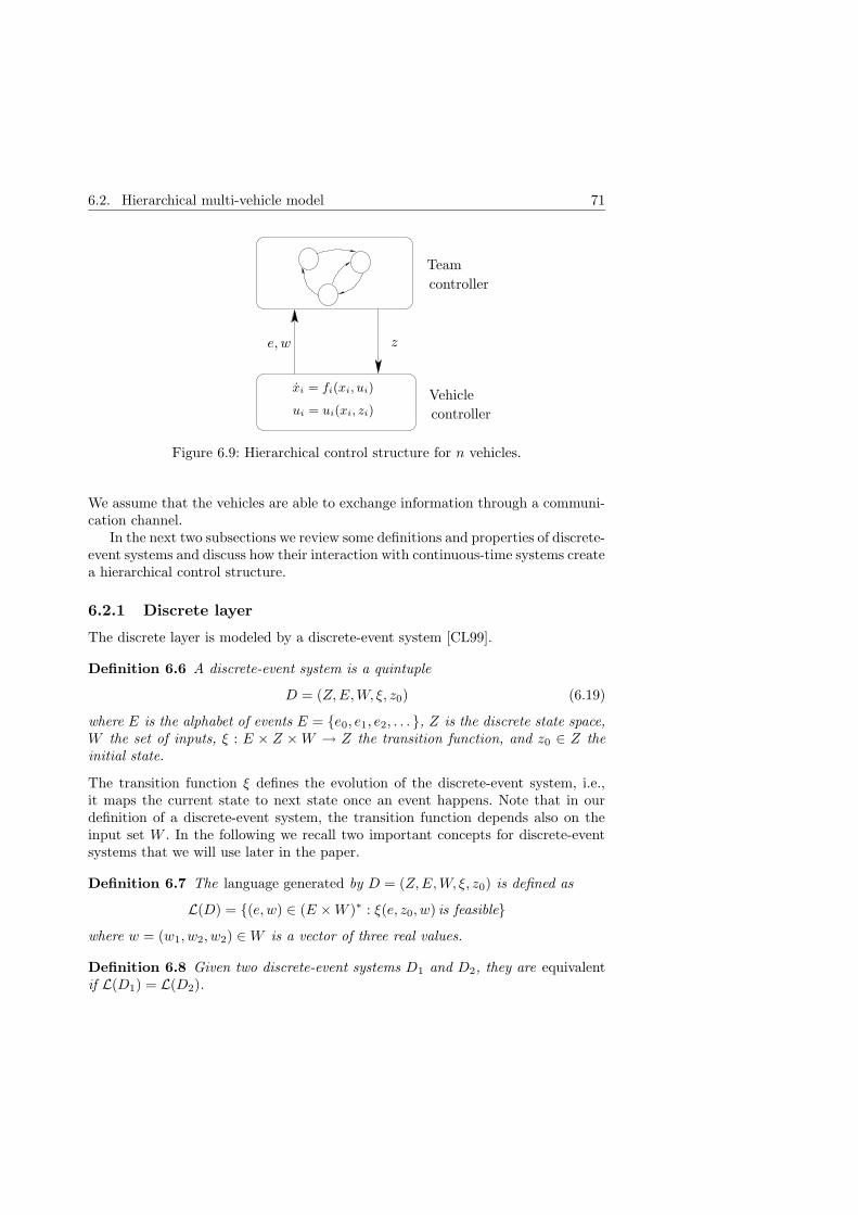
6.2. Hierarchical multi-vehicle model 71
PSfrag replacements
e, w z
xi = fi(xi, ui)
ui = ui(xi, zi)
Team
controller
Vehicle
controller
Figure 6.9: Hierarchical control structure for n vehicles.
We assume that the vehicles are able to exchange information through a communi-cation channel.
In the next two subsections we review some definitions and properties of discrete-event systems and discuss how their interaction with continuous-time systems createa hierarchical control structure.
6.2.1 Discrete layer
The discrete layer is modeled by a discrete-event system [CL99].
Definition 6.6 A discrete-event system is a quintuple
D = (Z,E,W, ξ, z0) (6.19)
where E is the alphabet of events E = e0, e1, e2, . . . , Z is the discrete state space,W the set of inputs, ξ : E × Z ×W → Z the transition function, and z0 ∈ Z theinitial state.
The transition function ξ defines the evolution of the discrete-event system, i.e.,it maps the current state to next state once an event happens. Note that in ourdefinition of a discrete-event system, the transition function depends also on theinput set W . In the following we recall two important concepts for discrete-eventsystems that we will use later in the paper.
Definition 6.7 The language generated by D = (Z,E,W, ξ, z0) is defined as
L(D) = (e, w) ∈ (E ×W )∗ : ξ(e, z0, w) is feasiblewhere w = (w1, w2, w2) ∈W is a vector of three real values.
Definition 6.8 Given two discrete-event systems D1 and D2, they are equivalentif L(D1) = L(D2).

72 References
6.2.2 Continuous layer
The continuous layer represents the dynamics of the vehicles and the continuous-time control algorithms. Each vehicle i = 1, . . . , n is described by a control system
xi = fi(xi, ui), ui ∈ Ui
where fi : Xi × Ui → Ω defines the dynamics of the individual vehicles with con-tinuous state xi and admissible continuous controls in Ui. The control ui is a statefeedback that depends on both the continuous state and the state of the discrete-event system in the discrete layer zi i.e.,
ui = ui(xi, zi).
The interactions between the two layers are described in the following.
6.3 Team controller
The search strategy described in this paper is based on the simplex algorithmwhich we describe in some detail in the next subsection. We then show how itis possible to design a team controller, modeled as a discrete-event system, thatexecutes the simplex algorithm. An equivalent implementation with communicatingteam controllers is then designed.
6.3.1 Simplex search
The simplex algorithm is a direct search method used in many practical optimiza-tion problems. It is usually applied in situations where the cost of function evalua-tion is high and gradient calculation is difficult, as happens in scalar field corruptedby noise or time-varying. The algorithm is useful to improve an initial estimate ofthe solution with few function evaluations. Its simplicity and robustness proper-ties [LRWW98, NM65], make it an interesting algorithm for minimum search appli-cations with multiple vehicles. Notice that the widely used gradient based methodscannot cope with the existence of noise in the field. Moreover, the main objectivein this kind of application is not an algorithm which converges in few iterations butone which enhances the synergy between the vehicles given the problem constraints.
Let us define a triangular grid G ∈ Ω as depicted in Figure 6.10, with apertured > 0. Introduce an arbitrary point p0 ∈ Ω and a base of vectors given by b1, b2such that bT1 b1 = bT2 b2 = d2 and bT1 b2 = d2 cosπ/3. The grid is then equal to
G = p ∈ Ω| p = p0 + kb1 + `b2, k, ` ∈ Z.
A simplex z = (z1, z2, z3) ∈ G3 is defined by three neighboring vertices of G, whichbelong to a triangle.

6.3. Team controller 73
PSfrag replacements
d
Figure 6.10: A triangular grid with aperture d over a two-dimensional scalar fielddepicted by its level curves. The solid line triangle illustrates the state z of thediscrete-event system evolving on the grid.
We suppose, without loss of generality, that V (z3) > V (zi), i = 1, 2. Given asimplex z = (z1, z2, z3) the next simplex, z′, is generated from z by reflecting z3with respect to the other vertices, namely
z 7→ z′ = S(z1, z2, z′3) z′3 = z1 + z2 − z3 (6.20)
where S(.) defines the following simplex algorithm:
1: z(0)← (z1(0), z2(0), z3(0))2: k ← 03: while true do4: i← arg maxi V (zi(k))5: z′i ← zj + zh − zi with j, h ∈ 1, 2, 3
and j 6= h, j 6= i, h 6= i6: z′j ← zj
7: z′h ← zh
8: z(k + 1)← (z′1, z′2, z
′3)
9: k ← k + 110: if k > 2 ∧ z(k) = z(k − 2) then11: stop12: end if13: end while
Notice that the algorithm terminates at time instance k = N with N > 2, ifz(N) = z(N−2). Since the algorithm is deterministic, it follows that a continuationafter step N would lead to an oscillation between the two discrete states z(N) andz(N − 1).
Definition 6.9 A fixed point χ for the simplex algorithm is a pair of two simplexesthat makes the algorithm to terminate. Thus
χ = (z(k − 1), z(k)
)∈ G3 × G3 : z(k − 2) = z(k), k > 2.
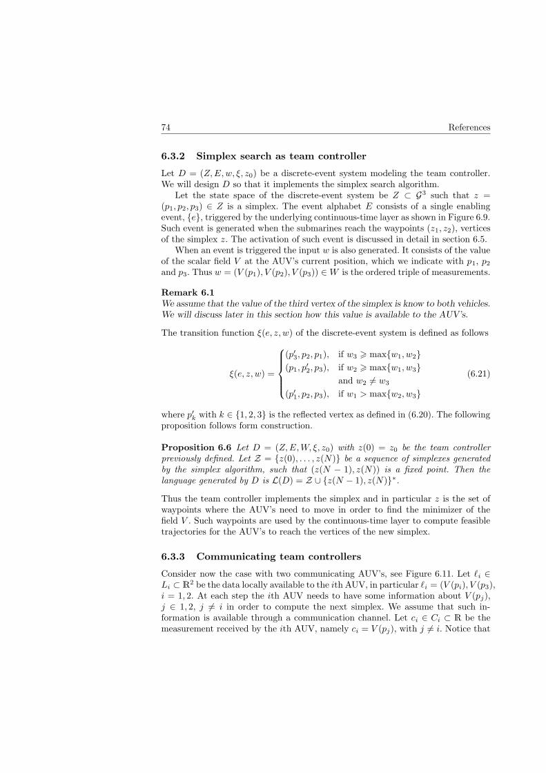
74 References
6.3.2 Simplex search as team controller
Let D = (Z,E,w, ξ, z0) be a discrete-event system modeling the team controller.We will design D so that it implements the simplex search algorithm.
Let the state space of the discrete-event system be Z ⊂ G3 such that z =(p1, p2, p3) ∈ Z is a simplex. The event alphabet E consists of a single enablingevent, e, triggered by the underlying continuous-time layer as shown in Figure 6.9.Such event is generated when the submarines reach the waypoints (z1, z2), verticesof the simplex z. The activation of such event is discussed in detail in section 6.5.
When an event is triggered the input w is also generated. It consists of the valueof the scalar field V at the AUV’s current position, which we indicate with p1, p2
and p3. Thus w = (V (p1), V (p2), V (p3)) ∈W is the ordered triple of measurements.
Remark 6.1We assume that the value of the third vertex of the simplex is know to both vehicles.We will discuss later in this section how this value is available to the AUV’s.
The transition function ξ(e, z, w) of the discrete-event system is defined as follows
ξ(e, z, w) =
(p′3, p2, p1), if w3 > maxw1, w2(p1, p
′2, p3), if w2 > maxw1, w3
and w2 6= w3
(p′1, p2, p3), if w1 > maxw2, w3
(6.21)
where p′k with k ∈ 1, 2, 3 is the reflected vertex as defined in (6.20). The followingproposition follows form construction.
Proposition 6.6 Let D = (Z,E,W, ξ, z0) with z(0) = z0 be the team controllerpreviously defined. Let Z = z(0), . . . , z(N) be a sequence of simplexes generatedby the simplex algorithm, such that (z(N − 1), z(N)) is a fixed point. Then thelanguage generated by D is L(D) = Z ∪ z(N − 1), z(N)∗.
Thus the team controller implements the simplex and in particular z is the set ofwaypoints where the AUV’s need to move in order to find the minimizer of thefield V . Such waypoints are used by the continuous-time layer to compute feasibletrajectories for the AUV’s to reach the vertices of the new simplex.
6.3.3 Communicating team controllers
Consider now the case with two communicating AUV’s, see Figure 6.11. Let `i ∈Li ⊂ R
2 be the data locally available to the ith AUV, in particular `i = (V (pi), V (p3),i = 1, 2. At each step the ith AUV needs to have some information about V (pj),j ∈ 1, 2, j 6= i in order to compute the next simplex. We assume that such in-formation is available through a communication channel. Let ci ∈ Ci ⊂ R be themeasurement received by the ith AUV, namely ci = V (pj), with j 6= i. Notice that

6.3. Team controller 75
PSfrag replacements
e, w z e, w z
x1 = f1(x1, u1)
u1 = u1(x1, z1)
x2 = f2(x2, u2)
u2 = u2(x2, z2)
D1 D2Channel
Team controllerTeam controller
Vehicle controller Vehicle controller
Figure 6.11: Decentralized hierarchical control structure for n = 2 vehicles with acommunication channel.
when the two AUV’s have exchanged measurements they have available the data(li, ci).
We, then,define the following two team controllers that generate waypoints forthe AUV’s
Di =(Z,Ei, (Li, Ci), ξi, z0
), i = 1, 2 (6.22)
The event alphabet contains a common enabling event, triggered by the continuous-time layer, thus Ei = e. In other words, the two AUV’s observe the same enablingevent e which is triggered when both vehicles have reached their previously com-puted waypoint. The transition function ξi is defined as follows
ξ1(e, z1, (`1, c1)) =
(p′3, p2, p1), if V (p3) > maxV (p1), c1(p1, p
′2, p3), if c1 > maxV (p1), V (p3)
and c1 6= V (p3)
(p′1, p2, p3), if V (p1) > maxV (p3), c1
(6.23)
and,
ξ2(e, z2, (`2, c2)) =
(p′3, p2, p1), if V (p3) > maxV (p2), c2(p1, p
′2, p3), if V (p2) > maxV (p3), c2
and V (p2) 6= V (p3)
(p′1, p2, p3), if c2 > maxV (p2), V (p3)
(6.24)
76 References
Proposition 6.7 The team controller D and the team controller obtained by com-posing D1 and D2 are language equivalent: L(D) = L(D1‖D2).
The result follows by construction. The parallel composition of D1 and D2 is thediscrete-event system
Dp = D1‖D2 =(Z × Z, e, (L1 ∪ C1) ∪ (L2 ∪ C2), ξp, (z0, z0)
).
where the initial state z0 is the same simplex for both AUV’s. Note that (L1∪C1)∪(L2 ∪ C2) = W , defined as for the centralized scheme. Since the enabling event eis observed by both discrete-event system then the transition function ξp is definedas follows
ξp(e, (z1, z2), w) =(ξ1(e, z1, w), ξ2(e, z2, w)
)
with w ∈ W and where (z1, z2) ∈ Z × Z. Since the AUV’s know the position ofeach other and ξ1 = ξ2 it follows that if the initial condition z0 is the same for D1
and D2 then their future states are the same, i.e. z1(k) = z2(k) for all k > 0. Thisimplies that ξ(e, z1, w) = ξ(e, z2, w), thus ξp(e, (z1, z2), w) represents a single stateof Z. Then we conclude that L(Dp) = L(D).
Remark 6.2The team controllers specify how the discrete-event systems compute a new simplex.However, they do not define which AUV moves to the reflected point. Such decisionis implicitly defined by the transition functions ξi (cf. equations (6.23) and (6.24))if we interpret the next state ξi(e, zi, (`i, ci)) as an ordered tuple, namely the nextwaypoint for the ith AUV is the ith element of ξi(e, zi, (`i, ci)), with i = 1, 2.
6.4 Communication issues
Underwater communication is very costly in terms of energy since the SNR is gen-erally very low [PSRS01]. From the transition functions (6.23) and (6.24) we noticethat both AUV’s need to know the value of the field V at all the three vertices of thecurrent simplex in order to generate the next simplex. This is achieved transmit-ting measurement using underwater acoustic modems. We propose a communicationprotocols in which measurements and very short (in term of bits/symbols) synchro-nization codes are used. In doing this the average data rate is decreased compareto a protocol where the raw measurements are communicated.
If the communicated data are not available then the discrete event systems D1
and D2 are non-deterministic. This fact follows from that there are three possiblestates z′i = ξi(e, zi, (`i, ∅)), that can be reached.
We consider the following communication strategy. At each step the first AUVsends its measurement, V (p1) to the second. This AUV then replies using a messageγk depending on the comparison of the field’s value at the vertices of the currentsimplex. Summarizing we have

6.4. Communication issues 77
PSfrag replacements
p′3
p1
p2
p3V (p1)γ1
(a)
PSfrag replacements
p′3p1
p2
p3
V (p1)
γ1
p′3
p1
p2
p3V (p1)γ2
(b)
PSfrag replacements
p′3p1
p2
p3
V (p1)
γ1
p′3p1
p2
p3
V (p1)
γ2
p′3
p1
p2
p3V (p1)γ3
(c)
Figure 6.12: Motion of the AUV’s and communicated date for two different sce-narios. In dotted line is shown the current simplex. With the arrowed solid lineis represented the communication of raw measurement, while with a dashed lineis represented the transmission of a message. In deash-dotted line is shown thetrajectory of the AUV’s toward the destination vertexes.
message conditionγ1 V (p3) is the largestγ2 V (p2) is the largestγ3 V (p1) is the largest
The messages γk need tp be designed very small, in term of bits/symbols, comparedwith a measurement.
Observe that the second AUV, after receiving V (p1), knows the field’s value atall vertices of the current simplex, thus it can determine uniquely the message γk,k = 1, . . . , 3.
The team controllers require the AUV’s to know the value of the field V at thecommon point p3 at each step. The communication strategy suggested, implicitlyassigns the role of master to one of the two AUV’s. Thus this constraint can berelaxed and it is necessary that only the master always knows the field’s value atthat point. We consider as example a possible case that could occur. Suppose V (p3)is the largest value. This case is shown in Figure 6.12(a). The field assumes largestvalue at p3. Thus the next simplex is p1, p2, p
′3. With the communication protocol
proposed, the vehicle in p2 receives the measurement taken by the vehicle in p1,namely V (p1), shown with a solid arrows line. At this point the vehicle in p2 hasall the measurements available and computes which vertex of the current simplexshould be reflected. The message γ3 is then communicate the the vehicle in p1. Thetransition functions ξi give
ξ2(e, p2, V (p1), V (p2), V (p3)) = (p′3, p2, p1)
78 References
and,
ξ1(e, p1, V (p1), γ3, V (p3)) = (p′3, p2, p1).
Thus the next simplex is the ordered triple (p′3, p2, p1). This means that vehicle inp1 will need to move to p′3 and vehicle p2 should remain standing still.
At the next step the value of V (p1) is known only to the vehicle in p2, butafter the communication of V (p′3) it can compute which of the vertexes should bereflected and transmit back the corresponding message.
The other two cases, shown in Figure 6.12(b) and Figure 6.12(c), follow similarly.
6.5 Vehicle controller
A complete nonlinear model of a Autonomous Underwater Vehicles can be foundin [Fos94]. In this work we consider the problem of controlling the AUV’s on aplane. The nonlinear model of the system is
xi = V cosψi
yi = V sinψi
ψi = ri i = 1, 2
where (xi, yi)T is the position of the ith AUV with respect to a global coordinate
frame, ψi is the yaw angle and ri is the yaw rate. The velocity V is assumed constant.The guidance in the horizontal plane is achieved using a “line of sight” control law:at each time step the vehicle is commanded to head towards the reference waypointzi. The continuous-time controller for the yaw is a PID
ri(xi, zi) = kpεi + ki
∫ t
0
εi(τ)dτ − kd
dψi
dt
where
εi = ∠(zi − (xi, yi)T )− ψi
The event e is generated when the vehicles reach the assigned waypoints. Dueto the vehicles’ control limitations, in practice, it is not possible to assure that thevehicles will reach the exact waypoint. To overcome this difficulty, when a vehiclereaches a neighborhood of radius δ of the assigned vertex of the simplex, a newmeasurement is taken and the event e is triggered. Therefore, the values are notalways sampled at the exact grid intersections. Additionally, position estimationerrors may lead to sampling being done even further from the desired point. MonteCarlo simulations, reported in the following section, have been performed in orderto test the robustness properties of the algorithm performing.
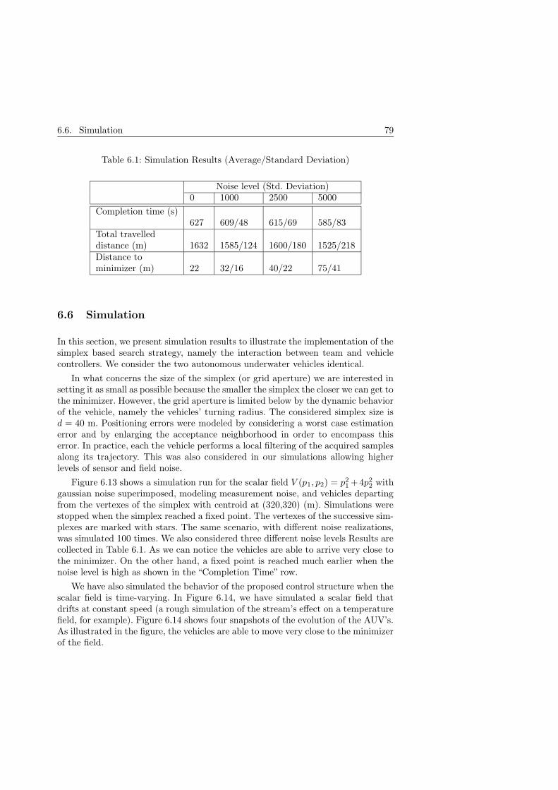
6.6. Simulation 79
Table 6.1: Simulation Results (Average/Standard Deviation)
Noise level (Std. Deviation)0 1000 2500 5000
Completion time (s)627 609/48 615/69 585/83
Total travelleddistance (m) 1632 1585/124 1600/180 1525/218Distance tominimizer (m) 22 32/16 40/22 75/41
6.6 Simulation
In this section, we present simulation results to illustrate the implementation of thesimplex based search strategy, namely the interaction between team and vehiclecontrollers. We consider the two autonomous underwater vehicles identical.
In what concerns the size of the simplex (or grid aperture) we are interested insetting it as small as possible because the smaller the simplex the closer we can get tothe minimizer. However, the grid aperture is limited below by the dynamic behaviorof the vehicle, namely the vehicles’ turning radius. The considered simplex size isd = 40 m. Positioning errors were modeled by considering a worst case estimationerror and by enlarging the acceptance neighborhood in order to encompass thiserror. In practice, each the vehicle performs a local filtering of the acquired samplesalong its trajectory. This was also considered in our simulations allowing higherlevels of sensor and field noise.
Figure 6.13 shows a simulation run for the scalar field V (p1, p2) = p21 +4p2
2 withgaussian noise superimposed, modeling measurement noise, and vehicles departingfrom the vertexes of the simplex with centroid at (320,320) (m). Simulations werestopped when the simplex reached a fixed point. The vertexes of the successive sim-plexes are marked with stars. The same scenario, with different noise realizations,was simulated 100 times. We also considered three different noise levels Results arecollected in Table 6.1. As we can notice the vehicles are able to arrive very close tothe minimizer. On the other hand, a fixed point is reached much earlier when thenoise level is high as shown in the “Completion Time” row.
We have also simulated the behavior of the proposed control structure when thescalar field is time-varying. In Figure 6.14, we have simulated a scalar field thatdrifts at constant speed (a rough simulation of the stream’s effect on a temperaturefield, for example). Figure 6.14 shows four snapshots of the evolution of the AUV’s.As illustrated in the figure, the vehicles are able to move very close to the minimizerof the field.

80 References
6.7 Conclusions
In this paper we have considered the problem of finding the minimizer of a scalarfield using a team of autonomous underwater vehicles. We proposed a hierarchicalcontrol strategy in which the high level consists of a team controller, modeled asa discrete-event system, which generates waypoints according to the simplex algo-rithm. The low level consists of a vehicle controller which generates continuous-timecontrol commands that move the AUV’s between waypoints.
A communication protocol have been designed in order to reduce the averagebit-rate. Simulation results have been carried out to show how the hierarchicalcontrol system moves the AUV’s towards the minimizer of a time-invariant and atime-varying vector field.
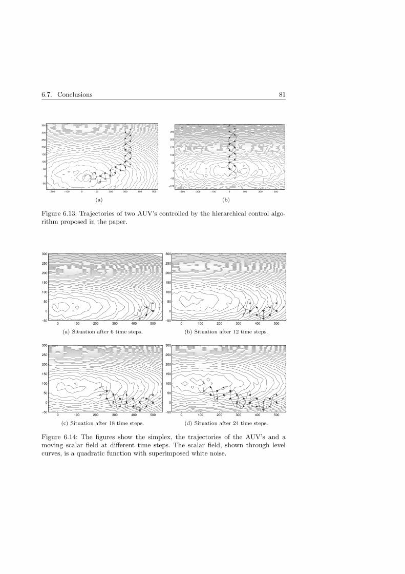
6.7. Conclusions 81
−200 −100 0 100 200 300 400 500
−50
0
50
100
150
200
250
300
350
(a)
−300 −200 −100 0 100 200 300
−100
−50
0
50
100
150
200
250
(b)
Figure 6.13: Trajectories of two AUV’s controlled by the hierarchical control algo-rithm proposed in the paper.
0 100 200 300 400 500−50
0
50
100
150
200
250
300
(a) Situation after 6 time steps.
0 100 200 300 400 500−50
0
50
100
150
200
250
300
(b) Situation after 12 time steps.
0 100 200 300 400 500−50
0
50
100
150
200
250
300
(c) Situation after 18 time steps.
0 100 200 300 400 500−50
0
50
100
150
200
250
300
(d) Situation after 24 time steps.
Figure 6.14: The figures show the simplex, the trajectories of the AUV’s and amoving scalar field at different time steps. The scalar field, shown through levelcurves, is a quadratic function with superimposed white noise.

References
[BL02] Ralf Bachmayer and Naomi Ehrich Leonard. Vehicle networks for gra-dient descent in a sampled environment. In IEEE Conference on De-cision and Control, 2002.
[BYBS96] E. Burian, D. Yoerger, A. Bradley, and H. Singh. Gradient search withautonomous underwater vehicles using scalar measurements. In IEEESymp. Autonomous Underwater Vehicle Technology, pages 86–89, 1996.
[CL99] C.G. Cassandras and S. Lafortune. Introduction to Discrete EventSystems. Kluwer Academic, 1999.
[CMdS+03] N. Cruz, A. Matos, J.B. de Sousa, F.L. Pereira, J. Silva, E.P. Silva,J. Coimbra, and E.B. Dias. Operations with multiple autonomousunderwater vehicles: the piscis project. In Proceedings of the SecondAnnual Symposium on Autonomous Intelligent Networks and Systems,2003.
[DLS95] N.G. Datta, J. Lygeros, and S. Sastry. Hierarchical hybrid control:a case study”, pages 166–190. Lecture Notes in Computer Science,Springer, 1995.
[dSP02] J. Borges de Sousa and Fernando Lobo Pereira. On coordinated con-trol strategies for networked dynamic control systems - an applicationto auvs. In Proceedings of International Symposium of MathematicalTheory of Networks and Systems (MTNS), 2002.
[Fos94] T. I. Fossen. Guidance and Control of Ocean Vehicles. John Wiley andSons Ltd., 1994.
[LRWW98] Jeffrey C. Lagarias, James A. Reeds, Margaret H. Wright, and Paul E.Wright. Convergence properties of the nedler-mead simplex in lowdimensions. SIAM Journal of Optimization, 9(1):112–147, 1998.
83
84 References
[McK99] K.I.M. McKinnon. Convergence of the nelder mead simplex method toa nonstationary point. SIAM Journal of Optimization, 148-158, 1999.
[NM65] J.A. Nelder and R. Mead. A simplex method for function minimization.Computing Journal, 7:308–313, 1965.
[PSRS01] J. Proakis, E. Sozer, J. Rice, and M. Stojanovic. Shallow water acousticnetworks. IEEE Communications Magazine, 39(11):114–119, 2001.
[SHH62] W. Spendley, G.R. Hext, and F.R. Himsworth. Sequential applica-tions of simplex designs in optimization and evolutionary operation.Technometrics, 4:441–461, 1962.
[Var72] P. Varaiya. Theory of hierarchical, multilevel systems. IEEE Transac-tion on Automatic Control, 17(2):280–281, 1972.
[Var00] P. Varaiya. A question about hierarchical systems. In In T. Djaferisand I. Schick, editors, System theory: modeling, analysis and control.Kluwer, 2000.

Paper C

On Some Communication Schemes
for Distributed Pursuit–Evasion
Games
A. Speranzon, K.H. Johansson
Abstract
A probabilistic pursuit-evasion game from the literature is used as an exampleto study constrained communication in multi-robot systems. Communication pro-tocols based on time-triggered and event-triggered synchronization schemes areconsidered. It is shown that by limiting the communication to events when theprobabilistic map updated by the individual pursuer contains new information, asmeasured through a map entropy, the utilization of the communication link can beconsiderably improved compared to conventional time-triggered communication.
Keyworkds: Probabilistic map, Relative entropy, Time- and Event-triggered com-munication.

7.1. Introduction 87
7.1 Introduction
Multi-robot systems have many advantages compared to single-robot systems, in-cluding improved flexibility, sensing, and reliability. For most mobile robot systems,one needs to address challenges related to sensor noise, self-localization, and partialknowledge of the environment. For a multi-robot system, the inter-robot commu-nication adds to this list. In practice, every communication channel has a limitedbandwidth, which is due to the physical laws on the achievable data rate and tothat channels might be shared with other users. The performance of the multi-robotsystem is often highly dependent on the utilization of the communication network.Still, integrated design of communication protocols has so far gained little attentionin the literature of multi-robot systems, cf., [BA94, TBF98].
The main contribution of this paper is to illustrate how information theory [Sha48,CT91] can be used in the design of a multi-robot system, in order to optimizethe communication utilization with respect to a control performance. We let apursuit–evasion game [Isa67, BO95, HKS99, HP02] with several pursuers serve asa prototype system, since it is a good representative for many multi-robot tasks.In particular we consider a probabilistic approach for pursuit–evasion where eachpursuer build a probabilistic map of the environment [HKS99, HKA00]. Map en-tropy is used as an information measure of the probabilistic map. It establishes anevent-triggered communication scheme for the pursuers, which is compared with atime-triggered scheme with periodic communications. The considered multi-robotproblem can be viewed as a realistic benchmark problem for the design of inte-grated control and communication systems. Recent work in that area has focusedmainly on stabilizability under limited communication, e.g., [WB99, Mit00]. Fora stochastic control system, the advantage of event-triggered control compared totime-triggered was discussed by Astrom and Bernhardsson [AB02]. For distributedreal-time systems, design specifications sometimes lead to that a time-triggeredscheme is instead preferable, as advocated by Kopetz [Kop93].
The paper is organized as follow. In Section 7.2 we extend the pursuit–evasionmodel of Hespanha et al. [HKS99] by introducing an explicit broadcasting com-munication protocol for the pursuer, in which they synchronize their probabilisticmaps by broadcasting the current map to each other. Two particular communica-tion schemes are discussed in Section 7.3: time-triggered and event-triggered. Thesynchronization events are in the latter based on the probabilistic map entropy. InSection 7.4 quantization is utilized to cope with bandwidth limitations. It is shownthat the map entropy can be used to quantize the probabilistic map in an efficientway. Simulation results are presented in Section 7.5.
7.2 Pursuit–Evasion with Communication
We consider a pursuit–evasion game with np > 1 pursuers, P1, . . . , Pnp, and one
randomly moving evader. Following Hespanha et al. [HKS99], we suppose that the
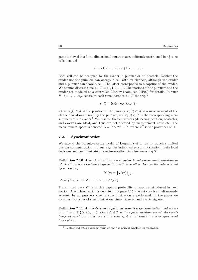
88 References
game is played in a finite-dimensional square space, uniformly partitioned in n2c <∞
cells denoted
X = 1, 2, . . . , nc × 1, 2, . . . , nc
Each cell can be occupied by the evader, a pursuer or an obstacle. Neither theevader nor the pursuers can occupy a cell with an obstacle, although the evaderand a pursuer can share a cell. The latter corresponds to a capture of the evader.We assume discrete time t ∈ T = 0, 1, 2, . . . . The motions of the pursuers and theevader are modeled as a controlled Markov chain, see [HP02] for details. PursuerPi, i = 1, . . . , np, senses at each time instance t ∈ T the triple
zi(t) = si(t),oi(t), ei(t)
where si(t) ∈ X is the position of the pursuer, oi(t) ⊂ X is a measurement of theobstacle locations sensed by the pursuer, and ei(t) ∈ X is the corresponding mea-surement of the evader2. We assume that all sensors (detecting position, obstacles,and evader) are ideal, and thus are not affected by measurement noise etc. Themeasurement space is denoted Z = X × 2X ×X , where 2X is the power set of X .
7.2.1 Synchronization
We extend the pursuit–evasion model of Hespanha et al. by introducing limitedpursuer communication. Pursuers gather individual sensor information, make localdecisions and communicate at synchronization time instances τ ∈ T .
Definition 7.10 A synchronization is a complete broadcasting communication inwhich all pursuers exchange information with each other. Denote the data receivedby pursuer Pi
Yi(τ) =yj(τ)
j 6=i
where yj(τ) is the data transmitted by Pi.
Transmitted data Y i is in this paper a probabilistic map, as introduced in nextsection. A synchronization is depicted in Figure 7.15: the network is simultaneouslyaccessed by all pursuers when a synchronization is performed. In the paper weconsider two types of synchronization: time-triggered and event-triggered.
Definition 7.11 A time-triggered synchronization is a synchronization that occursat a time τt ∈ ∆, 2∆, . . . , where ∆ ∈ T is the synchronization period. An event-triggered synchronization occurs at a time τe ∈ T , at which a pre-specified eventtakes place.
2Boldface indicates a random variable and the normal typeface its realization.
7.3. Entropy-triggered synchronization 89
7.2.2 Probabilistic Map
The probabilistic map for a pursuer is the probability mass function for the positionof the evader conditioned on the available data up to time t.
Definition 7.12 An element of the probabilistic map of pursuer Pi is given by
pit+1(xe, Zt) = P (xe(t+ 1) = xe|Zi
t = Zt) (7.25)
where Zit ∈ zi(0), . . . , zi(t), is the sequence of measurements taken by pursuer Pi
up to time t and xe(t) ∈ X is the position of the evader at time t.
The probabilistic map is a square matrix, where each element is given by equation(7.25). The map is updated through a two-step algorithm: a measurement stepin which P (xe(t) = xe|Zi
t = Zt) is computed using the current measurements,and a prediction step in which pi
t+1(xe, Zt) is computed using an evader motionmodel, see [HKS99] for details. The game starts with an a-priori probabilistic mappi0|−1(xe, ∅) that we assume to be the uniform distribution.
7.2.3 Control Policy
Let ui(t) denote the control action of Pi, which gives the position of Pi at timet+ 1. We consider greedy control policies with constrained motion for the pursuer,i.e.,
ui(t) = arg maxv∈N (si)
pit+1(v, Zt, Yt) (7.26)
where N (si) are all neighboring cells of the current position si of Pi. Thus, at t thecontrol policy moves Pi to a neighboring cell v, which maximizes the conditionalprobability of finding the evader at t+ 1. The greedy policy does not maximize thelocal probabilistic map pi
t+1, but the probabilistic map pit+1 which we let depend
also on the probabilistic maps received through the network; hence the greedypolicy (7.26) depends on the local measurement Zt and communicated data Yt. Thefusion of probabilistic maps at a synchronization time is computed as a normalizedproduct of all maps, i.e., as an independent opinion pool [Ber85]. This is basedon an assumption that the pursuers are far from each other between consecutivesynchronization instances. Measurements are thus considered to be approximatelyindependent, cf., [HK02].
7.3 Entropy-triggered synchronization
In this section we introduce an event-triggered synchronization scheme based onthe map entropy. We use the notation
mix(t) = pi
t+1(x, Zt, Yt)

90 References
PSfrag replacements
P1 Pi Pnp
Sync Sync Sync
Sync (period or event)
Y1(τ) Yi(τ)
y1(τ) yi(τ)
Ynp(τ)
ynp(τ)
Figure 7.15: At a synchronization time τ ∈ T , each pursuer Pi broadcasts yi(τ) tothe network and receives Yi(τ) = yj(τ)j 6=i.
for element x = (k, `) ∈ X of the probabilistic map of Pi and we letM i(t) denote thecorresponding matrix. Inspired by information theory [CT91] we make the followingdefinitions.
Definition 7.13 The map entropy H of a probabilistic map M is
H(M) = − 1
2 log nc
∑
x∈X
mx logmx
Definition 7.14 The relative map entropy D of two probabilistic maps M and Nis
D(M ||N) =∑
x∈X
mx logmx
nx
In particular, the relative map entropy between the probabilistic map M and theuniform probabilistic map N = n−2
c 1nc×ncis given by
D(M ||N) =1−H(M)
2 log nc
In the following we consider two event-triggered synchronization schemes: one basedon the map entropy and the other based on the relative map entropy.
7.3.1 Synchronization based on dynamic threshold
Let a synchronization event be triggered whenever H(M i(t)) < λ(t), where λ(t) isthe synchronization threshold. The threshold is updated according to
λ(t+ 1) =
α λ(τk), if t+ 1 = τk;λ(t), otherwise.
with λ(0) = λ0 > 0
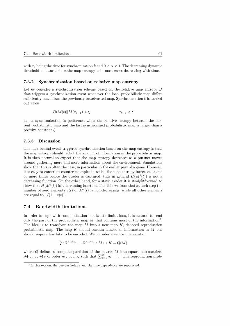
7.4. Bandwidth limitations 91
with τk being the time for synchronization k and 0 < α < 1. The decreasing dynamicthreshold is natural since the map entropy is in most cases decreasing with time.
7.3.2 Synchronization based on relative map entropy
Let us consider a synchronization scheme based on the relative map entropy Dthat triggers a synchronization event whenever the local probabilistic map differssufficiently much from the previously broadcasted map. Synchronization k is carriedout when
D(M(t)||M(τk−1) > ξ τk−1 < t
i.e., a synchronization is performed when the relative entropy between the cur-rent probabilistic map and the last synchronized probabilistic map is larger than apositive constant ξ.
7.3.3 Discussion
The idea behind event-triggered synchronization based on the map entropy is thatthe map entropy should reflect the amount of information in the probabilistic map.It is then natural to expect that the map entropy decreases as a pursuer movesaround gathering more and more information about the environment. Simulationsshow that this is often the case, in particular in the earlier part of a game. However,it is easy to construct counter examples in which the map entropy increases at oneor more times before the evader is captured; thus in general H(M i(t)) is not adecreasing function. On the other hand, for a static evader it is straightforward toshow that H(M i(t)) is a decreasing function. This follows from that at each step thenumber of zero elements z(t) of M i(t) is non-decreasing, while all other elementsare equal to 1/(1− z(t)).
7.4 Bandwidth limitations
In order to cope with communication bandwidth limitations, it is natural to sendonly the part of the probabilistic map M that contains most of the information3.The idea is to transform the map M into a new map K, denoted reproductionprobabilistic map. The map K should contain almost all information in M butshould require less bits to be encoded. We consider a vector quantization
Q : Rnc×nc → R
nc×nc : M 7→ K = Q(M)
where Q defines a complete partition of the matrix M into square sub-matricesM1, . . . ,MN of order n1, . . . , nN such that
∑Ni=1 ni = nc. The reproduction prob-
3In this section, the pursuer index i and the time dependence are suppressed.
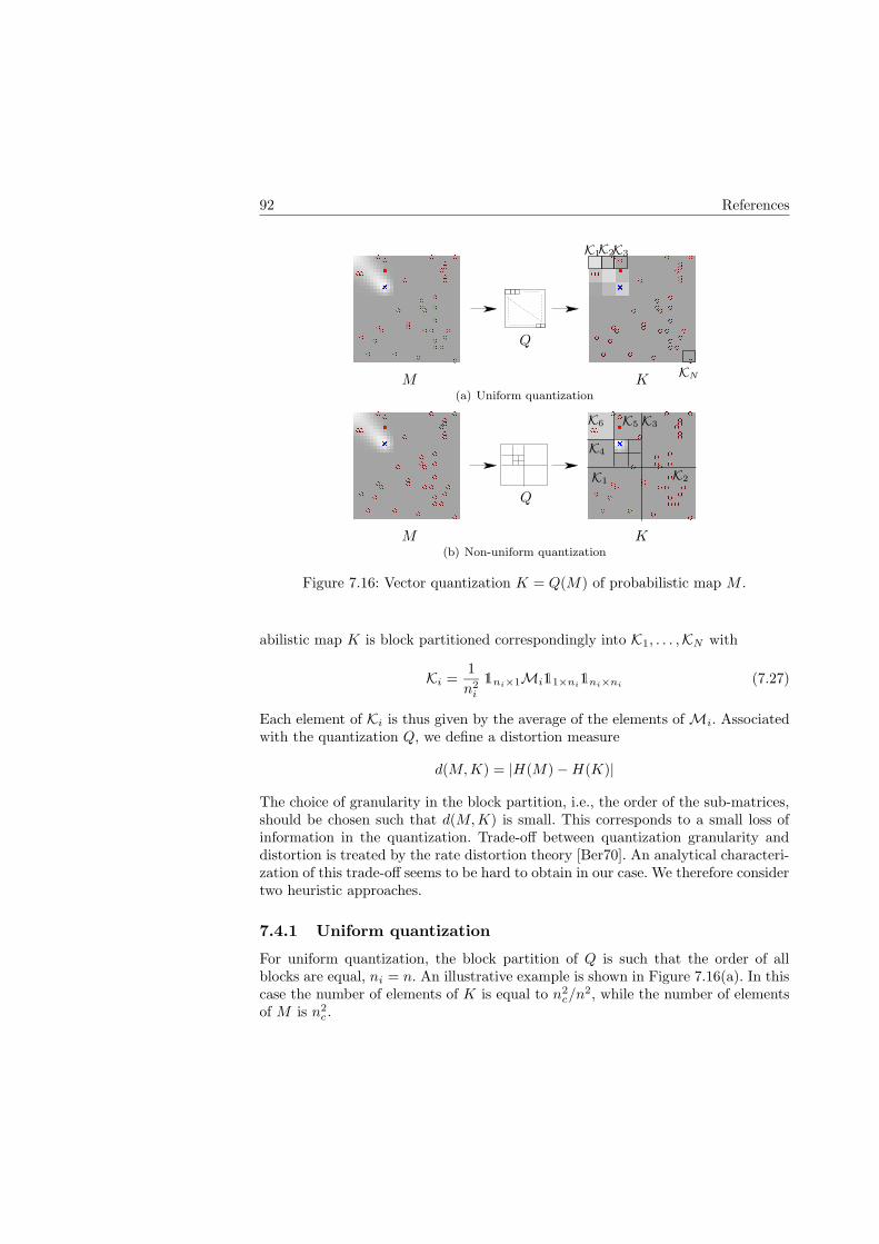
92 ReferencesPSfrag replacements
Q
M K
C
K1K2K3
KNK6
(a) Uniform quantization
PSfrag replacements
Q
M K
C
K1 K2
K3
KN
K6
K4
K5
(b) Non-uniform quantization
Figure 7.16: Vector quantization K = Q(M) of probabilistic map M .
abilistic map K is block partitioned correspondingly into K1, . . . ,KN with
Ki =1
n2i
1ni×1Mi11×ni1ni×ni
(7.27)
Each element of Ki is thus given by the average of the elements ofMi. Associatedwith the quantization Q, we define a distortion measure
d(M,K) = |H(M)−H(K)|
The choice of granularity in the block partition, i.e., the order of the sub-matrices,should be chosen such that d(M,K) is small. This corresponds to a small loss ofinformation in the quantization. Trade-off between quantization granularity anddistortion is treated by the rate distortion theory [Ber70]. An analytical characteri-zation of this trade-off seems to be hard to obtain in our case. We therefore considertwo heuristic approaches.
7.4.1 Uniform quantization
For uniform quantization, the block partition of Q is such that the order of allblocks are equal, ni = n. An illustrative example is shown in Figure 7.16(a). In thiscase the number of elements of K is equal to n2
c/n2, while the number of elements
of M is n2c .

7.5. Simulation results 93
7.4.2 Non-uniform quantization
A possible non-uniform quantization is illustrated in Figure 7.16(b). This corre-sponds to a “divide-and-conquer” scheme, which is known as vector quantizationwith QuadTree map [GG91]. The partitionM1, . . . ,MN imposed by the quantiza-tion Q is in this case carried out recursively, such that
dimM1 =1
4dimM
dimMi+1 =
dimMi, if i mod 3 = 0;14 dimMi, otherwise
(7.28)
In each recursion step, the current block is divided into four sub-matrices. Three ofthem are quantized using (7.27), while the remaining sub-block is partitioned intofour sub-blocks, and so on. The recursion stops when the smallest block has reacheda preassigned dimension n. Compared with uniform quantization, one advantage ofthe non-uniform quantization is the possibility of an on-line termination of thequantization if the loss of information is too high, i.e., if the distortion measured(M,K) is too large. Solving the recursion (7.28), we find that the number ofvalues to transmit is in the order of log n2
c + n2.
7.5 Simulation results
Sets of hundred Monte Carlo simulations have been performed in order to eval-uate the proposed synchronization and quantization strategies. The capture timeT ∗ and the number of synchronization instances S are used as performance in-dices. Figures 7.17 and 7.18 show the results for a game with two pursuers and oneevader on a grid with n2
c = 242 cells. Three different synchronization schemes arecompared: time-triggered, event–triggered based on dynamic threshold, and event-triggered based on relative map entropy. The time-triggered synchronization has asynchronization period of ∆ = 20. We see in Figure 7.17 that the capture time T ∗ isvarying considerably over the set of experiments. The mean capture time T
∗is sim-
ilar for all synchronization schemes as indicated by the dashed lines (dashed-dottedlines indicate the standard deviations). The result is collected in the following table:
Synchronization schemes T∗
STime-triggered 68 3.9Event-triggered dynamic threshold 64 2.1Event-triggered relative map en-tropy
66 2.6
Note that the mean number of synchronization times S is much smaller for theevent-triggered schemes than for the time-triggered, while the average capture timeT
∗is about the same. Hence, event-triggered synchronization allows a more efficient

94 References
utilization of the communication channel. This fact is also illustrated in Figure 7.18.The main difference between the two event-triggered schemes is mainly the distri-bution of synchronization times. We see that when using relative map entropy thepursuers tend to communicate more regularly. This is due to that new informa-tion is available quite regularly for the pursuers and this information triggers thesynchronization events in this scheme. In Figure 7.19 the uniform and non-uniformquantization strategies are compared. The results are for a game with two pursuersand one evader on an environment that consists of n2
c = 322 cells. The synchroniza-tion is time-triggered with period ∆ = 20. The quantization map Q has been chosenso that the dimension of the sub-matrices Ki is n2 = 82. Figure 7.19 shows T ∗ forthe following cases: no quantization (n = 1), uniform quantization with n = 8 andnon-uniform quantization with n = 8. The experimental results are collected in thefollowing table:
Quantization T∗
d(M,K) VUniform (n = 1) 91 0. 1024Uniform (n = 8) 141 0.1 16Non-uniform (n = 8) 120 0.04 70
Here d(M,K) denotes the average distortion over all experiments and V the averagenumber of broadcasted matrix elements at each synchronization. Note that V is oneto two magnitudes smaller for the quantized cases compared to the non-quantizedcase. Still the mean capture time is only about 50% larger. The uniform quantiza-tion compared with the non-uniform quantization has quite high average distortiond(M,K). This implies a relevant loss of information that makes T
∗larger in this
case. On the other hand the average number of transmitted data V is considerablyreduced.
7.6 Conclusions and future work
In this paper, we have presented communication protocols based on time-triggeredand event-triggered synchronization for a distributed pursuit–evasion game. Theevent-triggered schemes were based on the entropy of the probabilistic map. Simu-lations showed that by limiting the communication to certain events, the utilizationof the communication link can be considerably improved compared to conventionaltime-triggered communication with uniformly distributed synchronization times.Two vector quantization maps were considered in order to cope with bandwidthlimitations. A distortion measure based on the map entropy was introduced toevaluate the compression of the probabilistic map. The communication schemes de-veloped in the paper can be applied in cases when a probabilistic map has to be sentthrough a network channel to a decision maker. This is common in mobile robotics:examples include localization of robots using occupancy grids [ME85, TBF98]. Arelated problem of our current interest is optimal localization of mobile sensors,
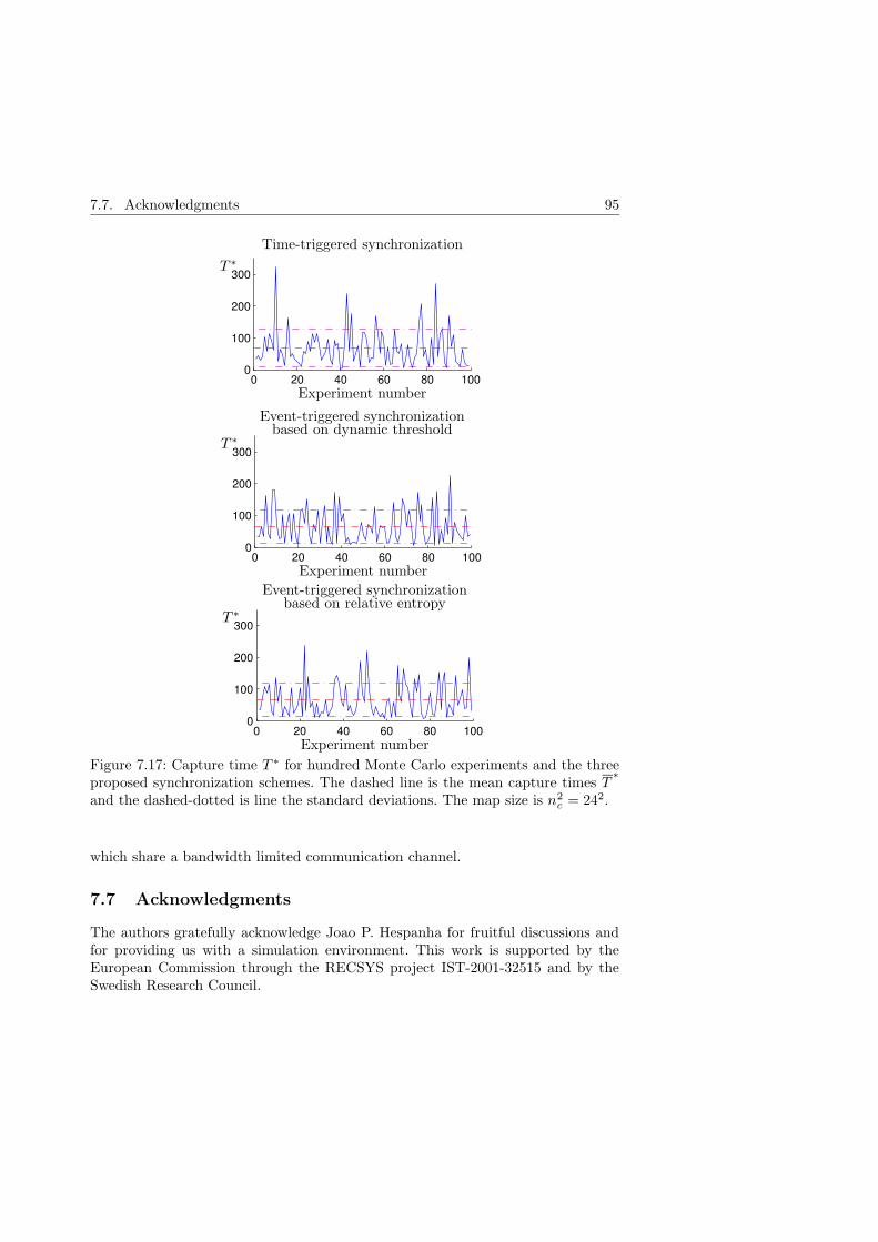
7.7. Acknowledgments 95
0 20 40 60 80 1000
100
200
300
0 20 40 60 80 1000
100
200
300
0 20 40 60 80 1000
100
200
300PSfrag replacements
T ∗
T ∗
T ∗
Time-triggered synchronization
Event-triggered synchronizationbased on dynamic threshold
Event-triggered synchronizationbased on relative entropy
Experiment number
Experiment number
Experiment number
Figure 7.17: Capture time T ∗ for hundred Monte Carlo experiments and the threeproposed synchronization schemes. The dashed line is the mean capture times T
∗
and the dashed-dotted is line the standard deviations. The map size is n2c = 242.
which share a bandwidth limited communication channel.
7.7 Acknowledgments
The authors gratefully acknowledge Joao P. Hespanha for fruitful discussions andfor providing us with a simulation environment. This work is supported by theEuropean Commission through the RECSYS project IST-2001-32515 and by theSwedish Research Council.
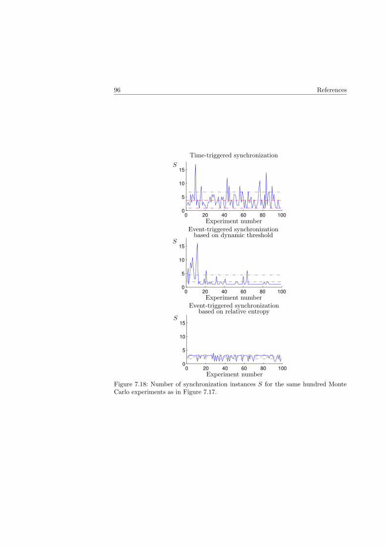
96 References
0 20 40 60 80 1000
5
10
15
0 20 40 60 80 1000
5
10
15
0 20 40 60 80 1000
5
10
15PSfrag replacements S
S
S
Time-triggered synchronization
Event-triggered synchronizationbased on dynamic threshold
Event-triggered synchronizationbased on relative entropy
Experiment number
Experiment number
Experiment number
Figure 7.18: Number of synchronization instances S for the same hundred MonteCarlo experiments as in Figure 7.17.

7.7. Acknowledgments 97
0 20 40 60 80 1000
200
400
600
800
0 20 40 60 80 1000
200
400
600
800
0 20 40 60 80 1000
200
400
600
800
PSfrag replacements
T ∗
T ∗
T ∗
Uniform quantization, (n = 1)
Uniform quantization, (n = 8)
Non-uniform quantization, (n = 8)
Trial number
Trial number
Trial number
Figure 7.19: Capture time T ∗ for hundred Monte Carlo experiments. In this casethe size of the map is n2
c = 322.


References
[AB02] K.J. Astrom and B.M. Bernhardsson. Comparison of Riemann andLebesgue sampling for first order stochastic systems. In IEEE Conferenceon Decision and Control, 2002.
[BA94] T. Balch and R.C. Arkin. Communication in reactive multiagent roboticsystems. Autonomous Robots, pages 27–52, 1994.
[Ber70] T. Berger. Rate distortion theory. Prentice-Hall, NJ, 1970.
[Ber85] J.O. Berger. Statistical decision theory and bayesian analysis. Springer-Verlag, Berlin, 1985.
[BO95] T. Basar and J.G. Olsder. Dynamic noncooperative game theory. Aca-demic Press, 2nd edition, 1995.
[CT91] T.M. Cover and J.A. Thomas. Elements of information theory. WileyInterscience, 1991.
[GG91] A. Gersho and R.M. Gray. Vector quantization and data compression.Kluwer, 1991.
[HK02] J.P. Hespanha and H. Kizilocak. Efficient computation of dynamic prob-abilistic maps. In Mediterranean Conference on Control and Automation,2002.
[HKA00] J.P. Hespanha, H.H. Kizilocak, and Y.S. Ateskan. Probabilistic mapbuilding for aircraft-tracking radars. Technical report, University ofSouthern California, Los Angeles, CA, 2000.
[HKS99] J.P. Hespanha, H. J. Kim, and S. Sastry. Multiple-agent probabilisticpursuit–evasion games. In IEEE Conference on Decision and Control,volume 3, pages 2432–2437, 1999.
99

100 References
[HP02] JP. Hespanha and M. Prandini. Optimal pursuit under partial informa-tion. In Mediterranean Conference on Control and Automation, 2002.
[Isa67] R. Isaac. Differential Games. Robert E. Kriger Publisher Company, 2edition, 1967.
[Kop93] H. Kopetz. Should responsive systems be event triggered or time trig-gered? IEICE Transaction on Information and Systems, pages 1525–1532,1993.
[ME85] H.P. Moravec and A.E. Elfes. High resolution maps from wide anglesonar. In IEEE International Conference on Robotics and Automation,1985.
[Mit00] S.K. Mitter. Control with limited information: the role of systems theoryand information theory. IEEE Information Theory Society Newsletter,4(50):122–131, 2000.
[Sha48] C.E. Shannon. A mathematical theory of communication. Bell SystemTechnical Journal, 27:379–423,623–656, 1948.
[TBF98] S. Thrun, W. Burgard, and D. Fox. A probabilistic approach to con-current mapping and localization for mobile robots. Machine Learning,31:29–53, 1998.
[WB99] W.S. Wong and R.W. Brockett. Systems with finite communicationbandwidth constraints ii: stabilization with limited information feedback.IEEE Transaction on Automatic Control, 44(5):1049–1052, 1999.

Part III
Conclusions
101


Chapter 8Conclusions and future work
This chapter briefly summarizes the key ideas presented in the three papers. Eachsummary ends with some future research directions.
Paper A
In Paper A we have studied the rendezvous problem for a team of robots that com-municate over quantized channels. Two different types of communication channelsare considered: uniformly and logarithmically quantized. The second one is prefer-able since in general less bits need to be communicated compared to the uniformquantized. For a class of feasible communication topologies, control laws that solvesthe rendezvous problem are derived. A stochastic approximation of the logarithmicquantization as multiplicative noise is also considered. The analysis, limited to thecase of two vehicles, shows that when the quantization error becomes very large, theinformation communicated over logarithmically quantized channels does not affectthe control action of the vehicle that receives it.
The communication topologies seem to influence the performances, for examplethe speed of convergence to the rendezvous point. A theoretical analysis that wouldallow the comparison between topologies seems to be a needed step. A possibleway to address this problem could be the stochastic approximation of the logarith-mic quantizer. Formation control under quantized communication, where complexgeometries are consider is a interesting future research direction. Furthermore wewould like to explore the possibility of having time-varying communication topolo-gies.
Paper B
A hierarchical control structure for a team of autonomous underwater vehicles em-ployed in finding the minimizer of a scalar field is discussed. The controller is com-
103

104 Chapter 8. Conclusions and future work
posed of two layers. The upper layer is the team controller which is modeled asdiscrete-event system. It generates waypoints based on the simplex search opti-mization algorithm. The waypoints are used as target points by the lower controllayer, which continuously steer each vehicle from the current to the next waypoint.Since underwater communication is costly in terms of energy, a protocol whichreduces the amount of data to be exchanged is also designed.
The hierarchical control structure seems to be promising for modeling multi-robot systems. The possibility of dividing the design problem in layers and includingthe communication as a part of the discrete layer seems to help in tackle the limita-tions it imposes in a easier way. Verification that specifications are fulfilled when wehave interaction among different layers is an important direction to be investigated.In particular specifications of interest regard the capability of the system to handlereconfiguration of the vehicles, to recover from faults in the communication and ve-hicles. In the paper we have studied only a particular example and a generalizationto other optimization algorithms would strength the framework.
Paper C
A distributed probabilistic pursuit–evasion game is considered in this paper. Theenvironment is divided in cells and a probabilistic map i.e., a map that associate toeach cell a value which is the probability the evader to be there, is constructed. Thepursuers can synchronize their probabilistic maps through a common communica-tion channel. The problem we address is the dependence of the capture time withthe frequency of the synchronization. Two different approaches are compared: time-triggered synchronization and event-triggered synchronization. The first is drivenby a clock with fixed frequency, the second depends on the information contentof the probabilistic map. Monte Carlo simulations show that the event-triggeredsynchronization do not increase the capture time despite the fact that the synchro-nization happens seldom. A discussion on how to cope with possible bandwidthlimitations during synchronization is also included.
There are many robotics problem where the robots build probabilistic maps.For example in mapping an environment or for navigation, occupancy grids arestill used. A possible future work direction could be the analysis of the proposedcommunication schemes in such applications. Further analysis is also needed forthe investigation of event-based and time-triggered communication. It would beinteresting to trade-off how often and how much you communicate.