1

On Clutter Ranks of Frequency Diverse RadarWaveforms

Yimin Liu, Member, IEEE, Le Xiao, Xiqin Wang, and Arye Nehorai, Fellow, IEEE

Abstract—Frequency diverse (FD) radar waveforms are attrac-tive in radar research and practice. By combining two typical FDwaveforms, the frequency diverse array (FDA) and the stepped-frequency (SF) pulse train, we propose a general FD waveformmodel, termed the random frequency diverse multi-input-multi-output (RFD-MIMO) in this paper. The new model can be appliedto specific FD waveforms by adapting parameters. Furthermore,by exploring the characteristics of the clutter covariance matrix,we provide an approach to evaluate the clutter rank of the RFD-MIMO radar, which can be adopted as a quantitive metric forthe clutter suppression potentials of FD waveforms. Numericalsimulations show the effectiveness of the clutter rank estimationmethod, and reveal helpful results for comparing the cluttersuppression performance of different FD waveforms.

Index Terms—Frequency diverse waveform, radar clutter,moving target indication, MIMO radar.

I. INTRODUCTION

WAVEFORM diversity has led to many interesting andpromising concepts in the research and practice of the

radar community in the past decade. By exploring waveformadaptivity in different domains, such as the spatial (antennabeampattern), temporal, spectral, code, and polarization do-mains, remarkable improvements have been realized in radarabilities, such as high resolution imaging, target recognition,clutter suppression, and electronic-counter-countermeasures(ECCM) [1]. Among the different kinds of diverse waveforms,frequency diverse (FD) waveforms are attractive due to theirease of use in system implementation [2], efficiency in wide-bandwidth synthesis [3], and robust in spectral compatibilityand resilience [4].

In 2006, a new array antenna, named the frequency diversearray (FDA), was introduced in [5]. By linearly [5] or ran-domly [6] (called LFDA or RFDA, respectively) assigning thecarrier frequencies of array elements, an FDA can providea beampattern which depends on both direction and range,and brings important benefits like transmit beamforming [7],target range-direction estimation [8], and jamming resistance[9], to list a few. Moreover, FDA-based algorithms enableadvantages in clutter or interference discrimination, and in

Y. Liu, L. Xiao, and X. Wang are with the Department ofElectronic Engineering, Tsinghua University, Beijing, 100084, China.e-mail: yiminliu@tsinghua.edu.cn, xiaol13@mails.tsinghua.edu.cn,wangxq ee@tsinghua.edu.cn.

A. Nehorai is with the Department of Electrical and Systems Engi-neering, Washington University, St. Louis, MO 63130 USA. e-mail: neho-rai@ese.wustl.edu.

The work of Y. Liu was supported by the National Natural ScienceFoundation of China (Grant No. 61571260 and 61201356). The work ofA. Nehorai was supported by the AFSOR (Grant No. FA9550-11-1-0210).Corresponding e-mail: yiminliu@tsinghua.edu.cn.

moving target detection. By using an FDA, the clutter inforward-looking radar was alleviated [10]. In [11], clutterwhose delay was outside of one pulse repetition interval (PRI)was successfully discriminated, hence the target detectionperformance of an airborne multi-input-multi-output (MIMO)radar was improved. However, quantitive metrics of FDAradars’ clutter suppression performance are still inadequate.

As defined in the IEEE Radar Standard P686/D2 (January2008), frequency diversity radar is “a radar that operates atmore than one frequency, using either parallel channels orsequential groups of pulses”. Following this definition, theFDA can be regarded as one kind of FD waveform that isdistributed in the spatial-spectral domain. Similarly, anotherkind of widely-used waveform, stepped-frequency (SF) pulsetrain [12], can be regarded as FD waveforms distributed inthe temporal-spectral domain. In the SF pulse train, the carrierfrequencies of pulses in a coherent processing interval (CPI)shift linearly [13] or randomly [14] (termed linear SF (LSF),or random SF (RSF)). Basic LSF pulse train can synthesize alarge bandwidth to achieve a very high range resolution [3].Furthermore, if the carrier frequencies of successive pulsesshift randomly, as in the RSF pulse trains, the ambiguity func-tions will become thumbtack-like, which implies an uncoupledhigh resolution in both range and velocity [3]. Moreover, theECCM performances of RSF radars are also outstanding, dueto its frequency agility [2].

Although some algorithms have been proposed for cluttersuppression [15] [16], the corresponding performance evalua-tions for the SF, especially RSF radars, still need research.In this paper, we try to provide general quantitive infor-mation about the clutter suppression potential of the FDradar waveforms. A new FD waveform model, named therandom-frequency-diverse-MIMO (RFD-MIMO), is proposedby integrating the FDA and SF pulse train. Because thecarrier frequencies of the array elements and pulses in RFD-MIMO vary agilely, the new waveform is diverse in a 3D(spatial-temporal-spectral) domain. Moreover, this model canbe applied to existing FD waveforms by adapting the modelparameters. Furthermore, the clutter rank, defined as the rankof a radar’s clutter covariance matrix (CCM), is evaluatedbased on this model. As introduced in [17] and [18], theclutter rank can quantify the averaged clutter suppressionperformance of a radar. Hence the results of this paper canbe regarded as a quantitive metric of the clutter suppressionpotential that can be achieved by the coherent processingof a frequency diversity radar. It should be noted that thisstudy focuses on coherent approaches to clutter suppression,and the intention is different from conventional works which

arX

iv:1

603.

0818

9v1

[cs

.IT

] 2

7 M

ar 2

016

2

Transmitted signal

dT dR

R receiving elementsL transmitting elements

Multi

Carrier

Receiver

Multi

Carrier

Receiver

Multi

Carrier

Receiver

Multi

Carrier

Receiver

Baseband samples

dT dR

Fig. 1. A brief schematic of an RFD-MIMO radar. Each brick corresponds to a pulse in the waveform, and different colors signify different carrier frequencies.The rows and columns of the bricks represent the pulses and transmitting elements, respectively.

employed the de-correlated radar cross section (RCS) responseproperties. In addition, unlike traditional clutter rank studies,such as [18] and [19], the main challenge encountered by thiswork was the disordered phase relationships between arrayelements and pulses, caused by the frequency diversity. Themain contributions of this paper are as follows.

1) We propose a general model, named RFD-MIMO, of FDradar waveforms. In this model, the carrier frequencyof each transmitting array element and each pulse canbe assigned an arbitrary value, and each receiving arrayelement can receive all the possible carrier frequenciessimultaneously.

2) We construct the target and clutter model of the RFD-MIMO waveform. Based on this model, we derive theexpressions of the FDA, SF, and FD-MIMO radars’clutter.

3) By exploring the features of an RFD-MIMO’s CCM,we derive an approximation of the new FD waveform’sclutter rank. We find that the frequency diversity radar’sCCM is sparse, and can be permuted to a block diagonalmatrix, which notably reduces the complexity of theclutter rank estimation.

4) We substantiate the clutter rank estimation of RFD-MIMO to specific FD radar waveforms, and quantifythe clutter suppression potentials of different frequencydiversity radars. The results reveal that, first, in radarsusing FDA or SF pulse trains, random carrier frequencyassignments have advantages in clutter suppression overtheir linear counterparts. Second, wideband pulses andMIMO antennas are more suitable for target detectionin heavy clutter scenarios.

The rest of this paper is organized as follows. Section IIpresents the radar schematic, and constructs the system andsignal models of the RFD-MIMO waveform. In Section III,by exploring the CCM, we derive an estimation approachfor the clutter rank of the new waveform. In Section IV,discussion and numerical results for radars with specific FDwaveforms are provided as substantiations of the providedmethod. Conclusions are drawn in the last section.

Notations: The important and frequently used notations are

TABLE IGLOSSARY OF NOTATIONS

Notation Discriptionc The speed of lightt The time variableZ The set of all integersC The set of all complex numbersfc The initial carrier frequency∆f The frequency incrementdT The distance between transmitting antenna elementsdR The distance between receiving antenna elementsT The pulse repetition interval (PRI)L The number of transmitting antenna elementsR The number of receiving antenna elementsP The number of pulses in a pulse trainG The frequency diverse code matrixGQ The augmented frequency diverse code matrix

with pulse bandwidth Q∆fMQ The set composed of all the unique entries in GQ

l The transmitting array element index vectorr The receiving array element index vectorp The pulse index vectorq The sub-band index vectorD The clutter range regionV The clutter velocity regionA The clutter direction sine regionC The clutter rankLFD The frequency diversity loss (FDL)R{·} The rank of a matrixvec{·} Column vectorization of a matrix[·]a,b The ath row, bth column entry of a matrix[·]a The ath entry(column) of a vector(matrix)| · | The number of unique elements of a vector/matrix/set| · |2 The l2-norm of a scalar/vector〈·〉 The difference between the maximum and minimum

entries in a vector/matrix/setb·c The largest integer which is no larger than an argumentd·e The smallest integer which is no less than an argument(·)T , (·)H The transpose and Hermitian of an argument(·)∗ The element-wise complex conjugation of an argumentI‖m{·} The column vector composed of row indices corresponding

to a vector/matrix’s entries which equal to mI=m{·} The column vector composed of column indices

corresponding to a vector/matrix’s entries which equal to m1A×B An A×B matrix (vector) with all-one entries⊗, � The Kronecker and Hadamard products~ The Khrati-Rao product⊕ The stretched sum (defined in Section II)

listed in Table I.

3

II. SYSTEM AND SIGNAL MODELS

In this section, we first formulate the RFD-MIMO radarwaveform as a general model of FD waveforms, and then givethe expression of the echoes from targets and clutter for theRFD-MIMO and specific frequency diversity radars.

A. General Model

As introduced in [6], the FDA can be regarded as anFD waveform which is distributed in the spatial-spectraldomain. Beyond this, we introduce a pulse train into thewaveform to expand it from 2D (spatial-spectral) diversity to3D (spatial-temporal-spectral) diversity. The system schematicof a radar with RFD-MIMO waveform is shown in Fig.1. In the RFD-MIMO radar, the transmitting and receivingantennas are colocated. There are L array elements, indexedby l = 0, 1, . . . , L − 1, in the transmitting antenna, andR array elements, indexed by r = 0, 1, . . . , R − 1, in thereceiving antenna. The elements in both antennas are equallyseparated, with the inter-element distances of the transmittingand receiving antennas being dT and dR, respectively.

In the RFD-MIMO radar, every transmitting element canbe assigned an arbitrary carrier frequency which is chosenfrom a candidate frequency set. The carrier frequency of everyelement can (but is not necessarily required to) vary frompulse to pulse. Thus a carrier frequency in the waveform isequal to an initial frequency (fc) plus an integral multiple of afrequency increment (∆f ). The integer is named the frequencydiverse code (FDC), and for all the P pulses (indexed byp = 0, 1, . . . , P − 1) in the pulse train, there are PL integers,which can be arranged into a frequency diverse code matrix(FDCM), G ∈ ZP×L. Then the carrier frequency transmittedby the lth array element in the pth pulse is

fp,l = fc + ∆f [G]p,l. (1)

For the signal of each pulse, both narrowband and widebandcases are considered. In narrowband cases, each pulse isassumed as monotone, with the same frequency as its carrierfrequency. In wideband cases, following the convention in[20], it is supposed that all the pulses have the same bandwidthB, which can be divided into Q sub-bands (Q is an integer,and B = Q∆f ); the signal of every sub-band can be regardedas a monotone multiplied by a modulation coefficient.

Then the transmitted signal of the pth pulse, lth arrayelement, and qth (q = 0, 1, . . . Q− 1) sub-band is

sp,l,q(t) = βp,l,q · exp(j2π(fc + ∆f([G]p,l + q)

)t), (2)

where βp,l,q is the modulation coefficient. According to (2), theFDCM can be expanded to an augmented-FDCM (a-FDCM),given by

GQ = G⊕ q, (3)

where q = [0, 1, . . . , Q− 1]T . In (3), ⊕ is the stretched sumoperator, where A⊕B = A⊗ 1size(B) + 1size(A) ⊗B 1.

1The definition of size(·) follows the eponymous MATLABr routine whichreturns the size of a matrix.

Transmitting ANT #0

R receiver columns

Transmitting ANT #1

R receiver columns

Transmitting ANT #L-1

R receiver columns

Pu

lse #

0P

uls

e #P

-1

P×Q

row

s

L blocks for transmitting elements

Q s

ub

ban

ds

Q s

ub

ban

ds

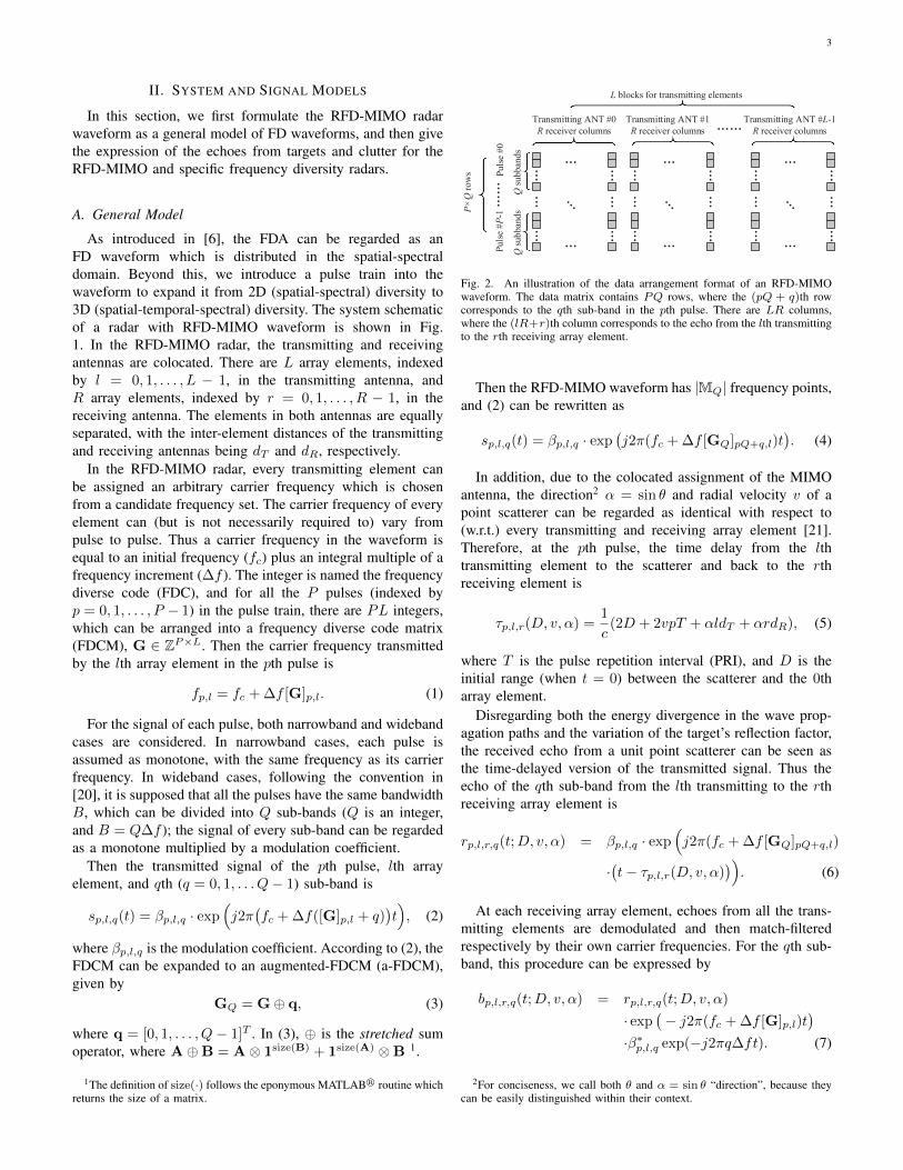
Fig. 2. An illustration of the data arrangement format of an RFD-MIMOwaveform. The data matrix contains PQ rows, where the (pQ + q)th rowcorresponds to the qth sub-band in the pth pulse. There are LR columns,where the (lR+r)th column corresponds to the echo from the lth transmittingto the rth receiving array element.

Then the RFD-MIMO waveform has |MQ| frequency points,and (2) can be rewritten as

sp,l,q(t) = βp,l,q · exp(j2π(fc + ∆f [GQ]pQ+q,l)t

). (4)

In addition, due to the colocated assignment of the MIMOantenna, the direction2 α = sin θ and radial velocity v of apoint scatterer can be regarded as identical with respect to(w.r.t.) every transmitting and receiving array element [21].Therefore, at the pth pulse, the time delay from the lthtransmitting element to the scatterer and back to the rthreceiving element is

τp,l,r(D, v, α) =1

c(2D + 2vpT + αldT + αrdR), (5)

where T is the pulse repetition interval (PRI), and D is theinitial range (when t = 0) between the scatterer and the 0tharray element.

Disregarding both the energy divergence in the wave prop-agation paths and the variation of the target’s reflection factor,the received echo from a unit point scatterer can be seen asthe time-delayed version of the transmitted signal. Thus theecho of the qth sub-band from the lth transmitting to the rthreceiving array element is

rp,l,r,q(t;D, v, α) = βp,l,q · exp(j2π(fc + ∆f [GQ]pQ+q,l)

·(t− τp,l,r(D, v, α)

)). (6)

At each receiving array element, echoes from all the trans-mitting elements are demodulated and then match-filteredrespectively by their own carrier frequencies. For the qth sub-band, this procedure can be expressed by

bp,l,r,q(t;D, v, α) = rp,l,r,q(t;D, v, α)

· exp(− j2π(fc + ∆f [G]p,l)t

)·β∗p,l,q exp(−j2πq∆ft). (7)

2For conciseness, we call both θ and α = sin θ “direction”, because theycan be easily distinguished within their context.

4

Substituting (6) into (7) gives the match-filtered sub-bandecho:

bp,l,r,q(D, v, α) = ‖βp,l,q‖22· exp

(− j 2π

c(fc + ∆f [GQ]pQ+q,l)

·(2D + 2vpT + αldT + αrdR)), (8)

which is time-invariant. In one pulse train, the number ofbaseband samples (termed the measurement dimension) isPQLR. All the PQLR samples can be arranged into a(PQ)×(LR) data matrix, whose (pQ+q)th row and (lR+r)thcolumn entry is bp,l,r,q(D, v, α). This data arrangement formatis illustrated in Fig. 2.

As shown in (8), the baseband echoes of an RFD-MIMOradar depend simultaneously on the scatterer’s range, ve-locity, and direction. Thus by vectorizing the data matrix,u(D, v, α) ∈ C(PQLR)×1 can be denoted as the range-velocity-direction steering vector, where

[u(D, v, α)](lR+r)PQ+pQ+q = bp,l,r,q(D, v, α). (9)

Furthermore, (8) also shows that the range-velocity-direction steering vector u(D, v, α) can be decomposed intothe Hadamard products of the modulation vector β, the rangesteering vector uD(D), the velocity steering vector uV(v), andthe direction steering vector uA(α):

u(D, v, α) = β � uD(D)� uV(v)� uA(α), (10)

where

[β](lR+r)PQ+pQ+q = ‖βp,l,q‖22,∀r = 0, 1, . . . , R− 1, (11)

uD(D) = vec{

exp(−j 4π

cD(fc+∆fGQ)⊗11×R)}, (12)

uV(v) = vec{

exp(− j 4π

cTv(fc + ∆fGQ

)�(p⊗ 1Q×L)⊗ (11×R)

)}, (13)

and

uA(α) = vec{

exp(− j 2π

cα(fc + ∆fGQ ⊗ 11×R)

�((dT1

PQ×1 ⊗ lT )⊕ (dRrT ))}. (14)

In the above equations, p = [0, 1 . . . , P − 1]T , l =[0, 1, . . . , L− 1]T , and r = [0, 1, . . . , R− 1]T .

In moving target indication (MTI) [2], clutter, which isdefined as the unwanted echo, is usually regarded as a super-imposition of received echoes from scatterers whose ranges,velocities, and directions are in a certain region (the clutterregion). In this work, we denote D, V, and A as the clutterrange, velocity, and direction regions, respectively. Hence theclutter echo vector can be calculated by

rC =

∫D

∫V

∫Aρ(D, v, α) · u(D, v, α)dDdvdα, (15)

where ρ(D, v, α) is the clutter reflection density of the range-velocity-direction coordinate {D, v, α}, as shown in Fig. 3.

The three-fold integral interval in (15) is determined asfollows.

V

The clutter

region

A

Direction

Velocity

Fig. 3. A simple illustration of the clutter range-velocity-direction region,and the clutter reflection density.

1) Clutter range region. Due to the clutter distribution fea-tures in practice [2] and the narrowband assumption ofeach sub-band, clutter is usually combined with echoesfrom scatterers located over a large range. However, ascan be seen in (12), the values of the range steering vec-tors are identical3 for scatterers with range differencesthat are multiples of c/(2∆f). Thus the clutter rangeregion is

D =[0,

c

2∆f

].

2) Clutter velocity region. Because the unambiguous targetvelocity is inversely proportional to the PRI in pulsedradars [2], the clutter velocity region should be a subsetof the unambiguous interval of velocity:

V ⊆[− c

4fcT,

c

4fcT

].

3) Clutter direction region. As introduced in [21], for a col-located MIMO radar, the clutter direction region shouldbe a subset of the unambiguous interval of direction:

A ⊆ [− c

2dRfc,

c

2dRfc].

Moreover, the integral in (15) can be approximated in adiscrete mode by summing up the echoes from all the voxelsin the clutter region. Assuming there are NC voxels, each ofwhich has a reflection amplitude ρn (n = 1, 2 . . . , NC), thenthe clutter echo vector can be re-written as

rC = C · ρ, (16)

where ρ = [ρ1, ρ2, . . . , ρNC]T , and C is the clutter steering

matrix (CSM), whose nth column is the steering vector of therange-velocity-direction coordinate {Dn, vn, αn}.

B. Application to Specific Frequency Diverse Waveforms

The system and signal model presented in last subsectioncan be applied to specific FD waveforms by adapting corre-sponding parts of the model, such as P , Q, L, R, dR, and GQ.Applications to FDA, SF, and frequency diverse MIMO (FD-MIMO) radar waveforms will be derived in this subsection.

3The phase factor −j4πfcD/c can be regarded as a part of the scatterer’sreflection amplitude, because it remains constant w.r.t. different p, q, r, andl.

5

1) FDA: In radars using FDA antennas, different arrayelements transmit and receive different carrier frequencieswhich can be shifted linearly [5] (linear FDA, LFDA ) orrandomly [6] (random FDA, RFDA). The range-directiondependent beampatterns are synthesized by processing thereceived echo.

In the FDA, the carrier frequencies of array elements arekept invariant throughout the operation. Thus the RFD-MIMOcan be applied by the following steps.

First, reduce the FDCM, G, to a row vector of L entries,gT . Second, if the signal of a single pulse is wideband, thea-FDCM will be expressed by

GQ = q⊕ gT . (17)

Because most research works about the FDA has focusedon the beampatterns, the system models are usually formulatedwith one pulse, which makes the target velocity unobservable.Thus in (13), the variable P should set to 1, and the velocitysteering vector uV(v) should be trivialized as an all-one vector.

Moreover, each array element in an FDA transmits andreceives with its own carrier frequency, thus in (5), l = r anddT = dR. In addition, the clutter direction region should beadapted to A ⊆ [−c/(4dRfc), c/(4dRfc)]. Hence the directionsteering vector can be expressed by

uA(α) = vec{

exp(− j 4π

cα(fc + ∆f(q⊕ gT )

)�(dT1

Q×1 ⊗ lT ))}. (18)

Finally, the integral in (15) should be calculated on only theclutter range region and clutter direction region. Therefore, theclutter model of an FDA radar is

rC =

∫D

∫Aρ(D,α) · β � uD(D)� uA(α)dDdα.

2) SF pulse train: The applications to LSF and RSF pulsetrains are straightforward. In radars with LSF or RSF pulsetrains, the antennas are usually configured as single-input-single-output (SISO). Thus the FDCM should be reduced to acolumn vector g with P entries, which represents the carrierfrequencies of all pulses in a pulse train. For pulses withbandwidth Q∆f , the a-FDCM is given by

GQ = g ⊕ q. (19)

The single element antenna makes the target’s directionunobservable in this instance. Hence in the waveform model,L = R = 1, dR = dR = 0, and the direction steering vectoruD(D) should be replaced by an all-one vector, 1(PQ)×1. Withthe above steps, the steering vectors of LSF and RSF pulsetrains are range-velocity dependent:

u(D, v) = β � uD(D)� uV(v), (20)

where

uD(D) = vec{

exp(− j 4π

cD(fc + ∆fg ⊗ q)

)},(21)

uV(v) = vec{

exp(− j 4π

cTv(fc + ∆fg ⊗ q)

�(p⊗ 1Q×1))}. (22)

Because it differs from that of an FDA radar, the clutterecho vector should be calculated by integrals on the clutterrange region and clutter velocity region:

rC =

∫D

∫Vρ(D, v) · β � uD(D)� uV(v)dDdv.

3) FD-MIMO and its space-time adaptive processing(STAP) applications: The MIMO technique has been appliedto the FDA waveform to improve the measurement dimension[20]. The FD-MIMO waveform is quite similar to the originalRFD-MIMO model. However, most researches on FD-MIMOis focused on the range-direction dependent beampattern.Therefore, the a-FDCM of an FD-MIMO waveform can bewritten as

GQ = q⊕ gT . (23)

As the steering vector, the application can be accomplishedby changing the velocity steering vector into an all-one vector,and removing the variable v from the parameters of thesteering vector.

However, in ground moving target indication (MTI) applica-tions [17], such as space-time adaptive processing for airborneradars [11], the pulse train is introduced in the waveform,and the ground clutter’s spatial frequency is assumed tobe linearly proportional to the temporal frequency [17]. Forthe most commonly studied side-looking mode antennas, therelationship between the spatial and temporal frequencies is

v = α · vp, (24)

where vp is the platform velocity. Thus the velocity steeringvector can be embedded into the direction steering vector,and the clutter model of an FD-MIMO radar with STAPapplications can be formulated by substituting (24) into (15):

rC =

∫D

∫Aρ(D, 0, α)·β�uD(D)�uV(αvp)�uA(α)dDdα,

where A is the direction region covered by the array element.

III. CLUTTER RANK ESTIMATION

Clutter rank, defined as the rank of a radar’s CCM, is animportant parameter for the quantification of target detectionperformance in clutter environments [17], [18]. A small clutterrank relative to the whole measurement dimension means thatthe radar has a greater ability to suppress the clutter [18].In this section, we explore the futures of the RFD-MIMO’sCCM and CSM, and then give a theorem for the clutter rankestimation of the new waveform.

A. Features of the CCM and CSM

According to the definition of the CCM, we have that

RC = E{rCr

HC

}= CE

{ρρH

}CH . (25)

From the basic properties of matrices [22], the clutter rank isgiven by

C , R{RC}≤ min

{R{C},R

{E{ρρH}

}}≤ R{C}, (26)

6

which means the clutter rank of a radar is no larger than therank of its CSM. The equality in the third row of (26) is validif the covariance matrix of the clutter reflection amplitudes,E{ρρH}, is full rank. Furthermore, the rank of the CSM is

R{C} = R{CCH}

= R{ NC∑n=1

u(Dn, vn, αn)uH(Dn, vn, αn)}.

Then, the clutter rank estimation is relaxed to the rankestimation of the Gramian matrix of the CSM’s Hermitian.Moreover, the summation in the above equation can be calcu-lated by integrals on the clutter range, velocity, and directionregions:

CCH =

∫D

∫V

∫Au(Dn, vn, αn)uH(Dn, vn, αn)dDdvdα.

(27)By substituting (10) into (27), CCH can be decomposed

into the Hadamard products of four matrices:

CCH = (ββH)�∫DuD(D)uHD (D)dD︸ ︷︷ ︸

RD

�∫VuV(v)uHV (v)dv︸ ︷︷ ︸

RV

�∫AuA(α)uHA (α)dα︸ ︷︷ ︸

RA

= (ββH)�RD �RV �RA, (28)

where ββH is rank-1, and RD, RV, and RA are all(PQLR)× (PQLR) matrices. Moreover, with the followinglemma, it can be shown that the second component of (28),RD, has good features which can simplify the clutter rankestimation.

Lemma 1: The ath, bth entry of RD, [RD]a,b, is non-zero,if and only if

[GQ]Ir(a),Ic(a) = [GQ]Ir(b),Ic(b), (29)

where

Ir(x) = x− (PQ) · bx/(PQ)c,Ic(x) = bx/(PQ)c.

Proof: According to the definition of RD in (28),

[RD]a,b =

∫D[uD(D)]a[uD(D)]∗bdD

=

∫De−j

4πc DzdD,

where z ∈ Z and z = [GQ]Ir(a),Ic(a) − [GQ]Ir(b),Ic(b). If thecondition given in (29) is satisfied,

[RD]a,b =

∫ c2∆f

0

e−j4π∆fc D·0dD =

c

2∆f.

Otherwise, if

[GQ]Ir(a),Ic(a) 6= [GQ]Ir(b),Ic(b), (30)

z becomes a non-zero integer. According to the Cauchy’sintegral theorem [23],

[RD]a,b =

∫ c2∆f

0

e−j4π∆fc D·zdD = 0.

Lemma 1 is proven. �Lemma 1 and (28) mean that many entries of CCH are zero.

Meanwhile, because RD is symmetric, the rest of the non-zeroentries can be permuted into a block diagonal matrix by rowand column swapping, where each diagonal block correspondsto a frequency point, fc+m∆f (m ∈MQ). Moreover, becausethe rank of a matrix remains unchanged during the row andcolumn swapping, R{CCH} can be decomposed to the sumof several smaller matrices’ ranks:

R{CCH} =∑m∈MQ

R{RCm

}, (31)

where RCm is the diagonal block corresponding to the fre-quency point fc +m∆f .

0 50 100 150 200 250 300 350 400 450 500

Colu

mn I

ndex

0

50

100

150

200

250

300

350

400

450

500

Row Index

0 50 100 150 200 250 300 350 400 450 500

Colu

mn I

ndex

0

50

100

150

200

250

300

350

400

450

500

0.1

0.2

0.3

0.4

0.5

0.6

0.7

0.8

0.9

1

Fig. 4. An example of the entries’ magnitudes in CCH , before (upper half)and after (lower half) row and column swapping.

Fig. 4 shows an example for the sparse and symmetricfeatures of CCH . In this example, the RFD-MIMO waveformhad four different carrier frequencies and 16 monotone pulsesin one CPI. The numbers of transmitting and receiving arrayelements were four and eight, respectively. The upper half ofFig. 4 shows the entries’ magnitudes in the original CCH ,and the lower half displays those of the permuted matrix. Itcan be clearly seen that after the row and column swapping,the permuted CCH has a block diagonal structure of fourdiagonal blocks.

In accordance with the row and column swapping, eachRCm can be decomposed to a Hadamard product of twomatrices:

RCm = RVm �RAm , (32)

where

RVm =

∫VuVm(v)uHVm(v)dv, (33)

RAm =

∫AuAm(α)uHAm(α)dα. (34)

7

In (33-34), uVm and uAm are sub-velocity and sub-directionsteering vectors, given by

uVm(v) = exp(− j 4π

cv(fc +m∆f)

·((T bI

‖m(GQ)

Qc)⊗ 1R×1

)), (35)

uAm(α) = exp(− j 2π

cα(fc +m∆f)

·((dTI=

m(GQ))⊕ (dRr))). (36)

With above derivations, CCH can be expressed by smallmatrices, such as RVm and RAm , whose dimensions arenotably reduced from the original ones. In addition, eachRVm and RAm depends only on a single frequency point,fc + m∆f . These features allow the clutter rank estimationof a diverse waveform to be accomplished in a “frequencypoint by frequency point” manner, which greatly reduces thecomplexity of the original problem.

B. Rank Estimation

The integrals in (33) and (34) can be approximated in matrixform, by discretizing the clutter velocity region and clutterdirection region into NV velocity grids and NA direction grids,respectively:

RVm = CVmCHVm ,

RAm = CAmCHAm ,

where[CVm ]n = uVm(vn), n = 1, 2, . . . , NV, (37)

[CAm ]n = uAm(αn), n = 1, 2, . . . , NA. (38)

Take the rank estimation of RVm as an example. Accord-ing to the basic properties of matrices [22], R{RVm} =R{CVm}. Furthermore, (35) and (37) show that the columnsof CVm can be regarded as complex sinusoids sampled on themth temporal sampling aperture, which is defined as the setcomposed of all the unique entries in vector T bI‖m(GQ)/Qc,in increasing order.

Some characteristics of the sampling apertures shouldbe noted. First, if the a-FDCM has multiple non-identicalcolumns, the sampling apertures corresponding to differentfrequency points may overlap. Second, each sampling aperturecan be divided into sub-apertures by splitting two successivesampling instants into two sub-apertures when the gap betweenthese two instants is larger than the Nyquist sampling interval,c/(2(fc +m∆f)〈V〉). All the sub-apertures corresponding tothe frequency point, fc+m∆f , are gathered as a set, Tm(V).

From the above discussion, an approximation of R{RVm}can be provided with the help of prolate spheroidal wave func-tion (PSWF) theory [24]. According to PSWF theory, complexsinusoids, whose energies are mostly confined in a certain“time(T )-frequency(W )” region, can be well approximated bylinear combinations of dWT +1e orthogonal functions. In ourcase, the “frequencies” of the complex sinusoids, uVm(vn),vary in an extent of 2(fc + m∆f)〈V〉/c. The “time” should

Normalized Extent of Clutter Velocity Region0 0.1 0.2 0.3 0.4 0.5 0.6 0.7 0.8 0.9 1

Norm

alizedRank

0

0.1

0.2

0.3

0.4

0.5

0.6

0.7

0.8

0.9

1

|G| = 1

Linear, |G| = 4

Linear, |G| = 8

Linear, |G| = 16

Random, |G| = 4

Random, |G| = 8

Random, |G| = 16

Fig. 5. The normalized UVm and the ranks of RVm , for different normalizedextents of clutter velocity region.

be counted separately for every sub-aperture in the Tm(V).Then we have the following lemma.

Lemma 2: The rank of RVm can be approximated by

R{RVm} ≈ UVm , min{|I‖m{GQ}|, RVm(V), RVm(V)

},

(39)where

RVm(V) = d2c

(fc +m∆f)〈V〉〈T bI‖m{GQ}Q

c〉e+ 1, (40)

and

RVm(V) =∑

T ∈Tm(V)

d2c

(fc +m∆f)〈V〉〈T 〉e+ 1. (41)

In equation (39), the first and second terms in the functionmin{·} are needed because the maximal number of linearlydependent signals with identical sampling instants is no largerthan the number of the sampling instants, and cannot bereduced by introducing new sampling instants.

An example of R{RVm} and UVm is provided in Fig. 5. Inthis example, we formulated an RFD-MIMO waveform with32 transmitting array elements, 8 receiving array elements,and 128 monotone pulses. Both linear and random carrierfrequency assignments were considered. The numbers of car-rier frequencies were set as |G| = 1 (the fixed-frequencycase, expressed similarly hereinafter), 4, 8, and 16. In thissimulation, the extent of the clutter velocity region varied fromzero to one times the unambiguous extent of velocity. BothR{RAm} and UVm were normalized by the numbers of uniquesampling instants in the temporal sampling aperture, and areindicated by symbols and dotted/dashed lines, respectively.The different colors indicate to different carrier frequencynumbers. The circles and triangles represent linear and randomcarrier frequency assignments, respectively. In this simulation,the approximations given by Lemma 2 matched the true rankswell. In addition, other phenomena could be seen: The fixed-frequency waveforms had the smallest rank; the larger thecarrier frequency number, the faster the normalized rank grew;

8

Normalized Extent of Clutter Direction Region0 0.1 0.2 0.3 0.4 0.5 0.6 0.7 0.8 0.9 1

Norm

alizedRank

0

0.1

0.2

0.3

0.4

0.5

0.6

0.7

0.8

0.9

1

|G| = 1

Linear, |G| = 4

Linear, |G| = 8

Linear, |G| = 16

Random, |G| = 4

Random, |G| = 8

Random, |G| = 16

Fig. 6. The normalized UAm and the normalized ranks of RAm , for differentnormalized extents of clutter direction region.

and the ranks of random carrier frequency assignments weresmaller than those of the linear ones.

The rank estimation of RAm can be derived in a similarway. As shown in (36) and (38), the columns of CAm can beregarded as the discrete samples of complex sinusoids whose“frequencies” vary in an extent of (fc + m∆f)〈A〉/c. More-over, the sampling instants are distributed on the mth spatialsampling aperture, which is determined by 〈(dTI=

m{GQ})⊕(dRr)〉. The Nyquist sampling interval in the spatial domainis c/((fc +m∆f)〈AdR〉). Thus the sampling instants corre-sponding to fc +m∆f can be divided to sub-apertures, all ofwhich are gathered as a set, Sm(A). With the above definitions,we have the following lemma.

Lemma 3: The rank of RAm can be approximated by

R{RAm} ≈ UAm

, min{|(dTI=

m{GQ})⊕ (dRr)|, RAm(A),

RAm(A)}, (42)

where

RAm(A) = d1c

(fc +m∆f)〈A〉〈(dTI=m{GQ})⊕ (dRr)〉e+ 1,

(43)and

RAm(A) =∑

S∈Sm(A)

d1c

(fc +m∆f)〈A〉〈S〉e+ 1. (44)

An example of R{RAm} and UAm is given in Fig. 6.The simulation setup and legends are the same as those inFig. 5, except the pulse number is 32 and the transmittingelements number is 128. Although the system configurationswere similar to those of the simulation for R{RVm}, theresults were different. In this example, the clutter ranks corre-sponding to different carrier frequency numbers had only smalldifferences between each other, for both linear and randomcarrier frequency assignments.

The reason can be briefly explained as follows: In theMIMO antenna, the spatial sampling aperture of each fre-

quency point is the stretched sum of the transmitting aperture(dTI=

m{GQ}) and the receiving aperture (dRr). Because dTis usually several times larger than dR, the discontinuity ofentries in I=

m{GQ} leads to a wide gap between spatialsampling instants. Hence when 〈A〉 is small, the spatialsampling aperture begins to divide into small sub-apertures.These sub-apertures are composed of integer multiples ofR sampling instants, and the distances between neighboringsampling instants are dR. Therefore, the rank is approximatelyproportional to the number of sampling instants, regardless ofthe number and the assignment of carrier frequencies.

With Lemma 2 and Lemma 3, we have the following lemmafor the rank of RCm .

Lemma 4: The ranks of the diagonal blocks, RCm , satisfythe following inequalities:

UCm ≤ R{RCm} ≤ min{Km,UVmUAm}, (45)

whereUCm , min

{Km,UVm + UAm − 1

}, (46)

and Km is the dimension of RCm .Proof: The proof can be found in Appendix A. �With the above preparation, we deduce the following the-

orem for the clutter rank estimation of the RFD-MIMOwaveform:

Theorem 1: If the covariance matrix of the clutter reflectionamplitudes is full rank, then the clutter rank of an RFD-MIMOradar, C, satisfies the following inequalities:∑

m∈MQ

UCm ≤ C ≤∑m∈MQ

min{Km,UVmUAm}, (47)

where UVm , UAm , and UCm are defined in (39), (42), and (46),respectively.

Proof: The proof of Theorem 1 can be accomplishedstraightforwardly by combining (31) and Lemma 4. �

IV. APPLICATIONS AND DISCUSSION

Due to the flexible configuration of the a-FDCM, the RFD-MIMO waveform is a general model for FD waveforms whosecarrier frequencies can vary for different array elements and/orpulses. In this section, we will give the rank estimation forspecific kinds of FD waveforms by the corollaries of Theorem1.

A. Metrics of Clutter Suppression Performance

As concluded in [18], a higher clutter rank relative to themeasurement dimension means that the clutter spreads over alarger portion of the whole signal space, leaving fewer clutter-free dimensions for the target detection. In this section, wewill compare the normalized clutter rank (NCR, defined asthe clutter rank, C, normalized by the measurement dimension,PQLR) between different FD radar waveforms, to show thecorresponding clutter suppression potentials. The reasons forchoosing the NCR are as follows.

First, as explained in Appendix B, the SCNRopt, definedas the optimal output signal-to-clutter-noise-ratio which canbe achieved by linear filtering, is approximately proportional

9

to the target energy which is spread in the orthogonal com-plement of the CCM’s eigenspace:

SCNRopt ≈1

σ2‖P⊥RC

· u(D, v, α)‖22, (48)

where P⊥RCis the projection matrix.

Numerical investigations (not analytically proven yet)showed that the averaged (w.r.t. all the unambiguous extents oftarget range, velocity, and direction) target power distributedon the CCM’s eigenspace is linearly proportional to thenormalized clutter rank (NCR):

meanD,v,α

{‖P⊥RC

· u(D, v, α)‖22}∝ 1− C

PQLR. (49)

The result in (49) implies that the averaged SCNRopt can bepredicted by the difference between the quantity 1 and theNCR.

Furthermore, the frequency diversity loss (FDL), defined asthe ratio between the SCNRopt of an FD waveform and theSCNRopt of a fixed-frequency waveform, can be expressedby the NCR:

LFD ≈1− CFD/(PQLR)

1− C0/(PQLR), (50)

where LFD is the FDL, and CFD and C0 are the clutter ranksof the fixed-frequency and the FD waveforms for the sameclutter environment4.

B. Frequency Diverse Array

As introduced in subsection II-B1, the applications of theRFD-MIMO to FDA can be accomplished by adapting thematrix G to a row vector gT . Thus according to Theorem1, the clutter rank of an FDA radar can be evaluated by thefollowing corollary.

Corollary 1: (Frequency Diverse Array) For an FDA radarwith a clutter direction region A, the clutter rank is

C ≈∑m∈MQ

min{|I=m{q⊕ gT }|,

d2c

(fc +m∆f)〈dTI=m{q⊕ gT }〉 · 〈A〉e+ 1,∑

S∈Sm(A)

d2c

(fc +m∆f)〈A〉〈S〉e+ 1}. (51)

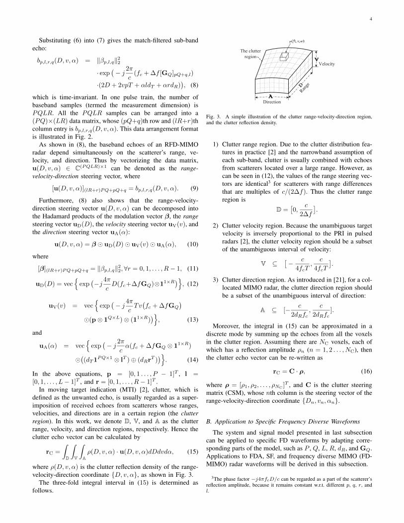
The NCRs of both LFDA and RFDA are illustrated in Fig.7. In this example, there were L = 256 array elements, andthe carrier frequency of each element was selected from aset of |G| = 1, 4, and 8 integers. Both monotone (Q = 1)and wideband (Q = 16) pulses were simulated. The clutterrank C and its approximation given in (51) were calculatedand then normalized by the measurement dimension PQLR.In the figure, the NCRs for different system configurationsare indicated by different symbols, and the approximationsare plotted by dashed and dotted lines for the LFDA and theRFDA, respectively.

4It should be noted that in this work, the clutter suppression is accomplishedby coherent processing, thus the results defer from the traditional incoherentcases. In addition, clutter whose delay is larger than one CPI is unconsidered.

Normalized Extent of Clutter Direction Region0 0.1 0.2 0.3 0.4 0.5 0.6 0.7 0.8 0.9 1

Norm

alizedRank

0

0.1

0.2

0.3

0.4

0.5

0.6

0.7

0.8

0.9

1

|G| = 1

Linear, Q = 1, |G| = 4

Linear, Q = 1, |G| = 8

Linear, Q = 16, |G| = 4

Linear, Q = 16, |G| = 8

Random, Q = 1, |G| = 4

Random, Q = 1, |G| = 8

Random, Q = 16, |G| = 4

Random, Q = 16, |G| = 8

Fig. 7. NCRs and their approximations for the FDA radar waveforms.

It is shown that the fixed-frequency (|G| = 1) waveformshave the lowest NCRs, and that the lower the carrier frequencynumber, the smaller the NCR. In addition, the NCRs ofwideband pulse waveforms (Q = 16) are much smaller thanthose of the monotone (Q = 1) ones. Furthermore, the LFDAhas a higher NCR than the RFDA, especially when 〈A〉 is inthe intermediate portion of the normalized extent of the clutterdirection region. This phenomenon will be further discussedin subsection IV-E, together with the SF pulse trains.

C. Stepped-Frequency Pulse Train

Coherent clutter suppression and moving target indicationare long-term problems for the SF, especially for the RSF(also known as frequency agile coherent [25]) radars [2]. WithTheorem 1, we can provide quantitative predictions of theclutter suppression performance for SF radars. According tothe appliaction steps given in subsection II-B2, we have thefollowing corollary.

Corollary 2: (Stepped-Frequency) For an SF radar withclutter velocity region V, the clutter rank is

C ≈∑m∈MQ

min{∣∣I‖m{g ⊕ q}

∣∣,d2c

(fc +m∆f)〈V〉〈T bI‖m{g ⊕ q}

Qc〉e+ 1,∑

T ∈Tm(V)

d2c

(fc +m∆f)〈V〉〈T 〉e+ 1}. (52)

The NCRs and their approximations for both the LSF andthe RSF radars are illustrated in Fig. 8. The pulse number was256, and the carrier frequency of each pulse was selected froma set of |G| = 1, 4, and 8 integers. Both monotone (Q = 1)and wideband (Q = 16) pulse waveforms were simulated.Results are shown with legends similar to those in Fig. 7.

The results revealed by Fig. 8 are analogous to Fig. 7: Fixed-frequency radars have the lowest NCRs; the higher the carrierfrequency number, the larger the NCR; the NCRs of widebandpulse waveforms are much smaller than those of monotone

10

Normalized Extent of Clutter Velocity Region0 0.1 0.2 0.3 0.4 0.5 0.6 0.7 0.8 0.9 1

Norm

alizedRank

0

0.1

0.2

0.3

0.4

0.5

0.6

0.7

0.8

0.9

1

|G| = 1

Linear, Q = 1, |G| = 4

Linear, Q = 1, |G| = 8

Linear, Q = 16, |G| = 4

Linear, Q = 16, |G| = 8

Random, Q = 1, |G| = 4

Random, Q = 1, |G| = 8

Random, Q = 16, |G| = 4

Random, Q = 16, |G| = 8

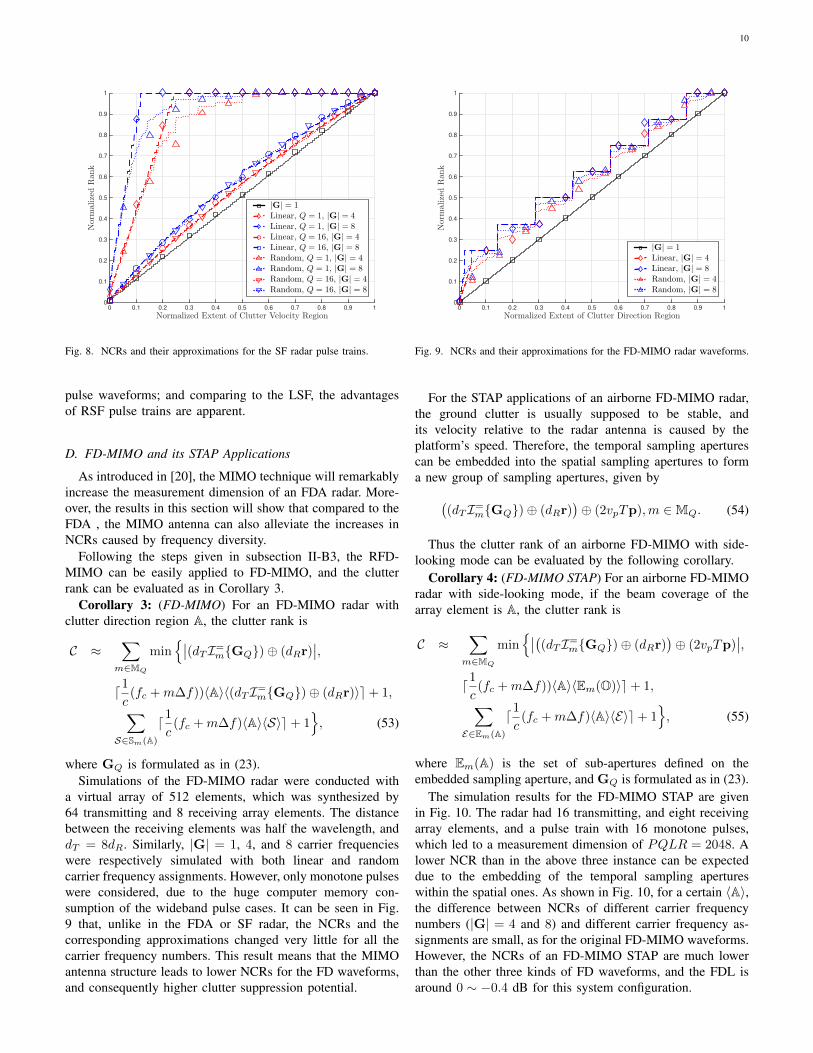
Fig. 8. NCRs and their approximations for the SF radar pulse trains.

pulse waveforms; and comparing to the LSF, the advantagesof RSF pulse trains are apparent.

D. FD-MIMO and its STAP Applications

As introduced in [20], the MIMO technique will remarkablyincrease the measurement dimension of an FDA radar. More-over, the results in this section will show that compared to theFDA , the MIMO antenna can also alleviate the increases inNCRs caused by frequency diversity.

Following the steps given in subsection II-B3, the RFD-MIMO can be easily applied to FD-MIMO, and the clutterrank can be evaluated as in Corollary 3.

Corollary 3: (FD-MIMO) For an FD-MIMO radar withclutter direction region A, the clutter rank is

C ≈∑m∈MQ

min{∣∣(dTI=

m{GQ})⊕ (dRr)∣∣,

d1c

(fc +m∆f))〈A〉〈(dTI=m{GQ})⊕ (dRr)〉e+ 1,∑

S∈Sm(A)

d1c

(fc +m∆f)〈A〉〈S〉e+ 1}, (53)

where GQ is formulated as in (23).Simulations of the FD-MIMO radar were conducted with

a virtual array of 512 elements, which was synthesized by64 transmitting and 8 receiving array elements. The distancebetween the receiving elements was half the wavelength, anddT = 8dR. Similarly, |G| = 1, 4, and 8 carrier frequencieswere respectively simulated with both linear and randomcarrier frequency assignments. However, only monotone pulseswere considered, due to the huge computer memory con-sumption of the wideband pulse cases. It can be seen in Fig.9 that, unlike in the FDA or SF radar, the NCRs and thecorresponding approximations changed very little for all thecarrier frequency numbers. This result means that the MIMOantenna structure leads to lower NCRs for the FD waveforms,and consequently higher clutter suppression potential.

Normalized Extent of Clutter Direction Region0 0.1 0.2 0.3 0.4 0.5 0.6 0.7 0.8 0.9 1

Norm

alizedRank

0

0.1

0.2

0.3

0.4

0.5

0.6

0.7

0.8

0.9

1

|G| = 1

Linear, |G| = 4

Linear, |G| = 8

Random, |G| = 4

Random, |G| = 8

Fig. 9. NCRs and their approximations for the FD-MIMO radar waveforms.

For the STAP applications of an airborne FD-MIMO radar,the ground clutter is usually supposed to be stable, andits velocity relative to the radar antenna is caused by theplatform’s speed. Therefore, the temporal sampling aperturescan be embedded into the spatial sampling apertures to forma new group of sampling apertures, given by(

(dTI=m{GQ})⊕ (dRr)

)⊕ (2vpTp),m ∈MQ. (54)

Thus the clutter rank of an airborne FD-MIMO with side-looking mode can be evaluated by the following corollary.

Corollary 4: (FD-MIMO STAP) For an airborne FD-MIMOradar with side-looking mode, if the beam coverage of thearray element is A, the clutter rank is

C ≈∑m∈MQ

min{∣∣((dTI=

m{GQ})⊕ (dRr))⊕ (2vpTp)

∣∣,d1c

(fc +m∆f))〈A〉〈Em(O)〉e+ 1,∑E∈Em(A)

d1c

(fc +m∆f)〈A〉〈E〉e+ 1}, (55)

where Em(A) is the set of sub-apertures defined on theembedded sampling aperture, and GQ is formulated as in (23).

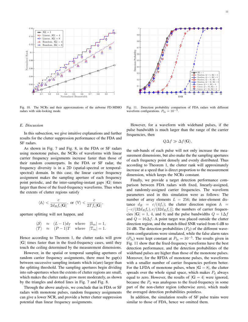
The simulation results for the FD-MIMO STAP are givenin Fig. 10. The radar had 16 transmitting, and eight receivingarray elements, and a pulse train with 16 monotone pulses,which led to a measurement dimension of PQLR = 2048. Alower NCR than in the above three instance can be expecteddue to the embedding of the temporal sampling apertureswithin the spatial ones. As shown in Fig. 10, for a certain 〈A〉,the difference between NCRs of different carrier frequencynumbers (|G| = 4 and 8) and different carrier frequency as-signments are small, as for the original FD-MIMO waveforms.However, the NCRs of an FD-MIMO STAP are much lowerthan the other three kinds of FD waveforms, and the FDL isaround 0 ∼ −0.4 dB for this system configuration.

11

Normalized Beamwidth0 0.1 0.2 0.3 0.4 0.5 0.6 0.7 0.8 0.9 1

Norm

alizedRank

0

0.02

0.04

0.06

0.08

0.1

0.12

0.14

0.16

|G| = 1

Linear, |G| = 4

Linear, |G| = 8

Random, |G| = 4

Random, |G| = 8

Fig. 10. The NCRs and their approximations of the airborne FD-MIMOradars with side-looking mode.

E. Discussion

In this subsection, we give intuitive explanations and furtherresults for the clutter suppression performance of the FDA andSF radars.

As shown in Fig. 7 and Fig. 8, in the FDA or SF radarsusing monotone pulses, the NCRs of waveforms with linearcarrier frequency assignments increase faster than those oftheir random counterparts. In the FDA or SF radar, thefrequency diversity is in a 2D (spatial-spectral or temporal-spectral) domain. In this case, the linear carrier frequencyassignment makes the sampling aperture of each frequencypoint periodic, and the inter-sampling-instant gaps |G| timeslarger than those of the fixed-frequency waveforms. Thus whenthe extents of clutter regions satisfy

〈A〉 < c

2dRfc|G|, or 〈V〉 < c

2Tfc|G|,

aperture splitting will not happen, and

〈S〉 ≈ (L− 1)dT where |Sm| = 1,〈T 〉 ≈ (P − 1)T where |Tm| = 1.

Hence according to Theorem 1, the clutter ranks will grow|G| times faster than in the fixed-frequency cases, until theytouch the ceiling determined by the measurement dimensions.

However, in the spatial or temporal sampling apertures ofrandom carrier frequency assignments, there must be gap(s)between successive sampling instants which is(are) larger thanthe splitting threshold. The sampling apertures begin dividinginto sub-apertures when the extents of clutter regions are small,which makes the clutter ranks grow more moderately, as shownby the triangles and dotted lines in Fig. 7 and Fig. 8.

Through the above analysis, we conclude that in FDA or SFradars with monotone pulses, random frequency assignmentscan give a lower NCR, and provide a better clutter suppressionpotential than linear frequency assignments.

SNR6 8 10 12 14 16 18 20 22 24

Det

ecti

on P

robab

lity

0

0.1

0.2

0.3

0.4

0.5

0.6

0.7

0.8

0.9

1

|G| = 1

Random, Q = 1, |G| = 4

Random, Q = 1, |G| = 8

Random, Q = 16, |G| = 4

Random, Q = 16, |G| = 8

Linear, Q = 1, |G| = 8

Linear, Q = 16, |G| = 4

Linear, Q = 16, |G| = 8

Fig. 11. Detection probability comparison of FDA radars with differentwaveform configurations. Pfa = 10−5.

However, for a waveform with wideband pulses, if thepulse bandwidth is much larger than the range of the carrierfrequencies, then

Q∆f � ∆f〈G〉,

the sub-bands of each pulse will not only increase the mea-surement dimensions, but also make the the sampling aperturesof each frequency point densely and evenly distributed. Thusaccording to Theorem 1, the clutter rank will approximatelyincrease at a speed that is direct proportion to the measurementdimension, which keeps the NCRs constant.

Finally, we provide a target detection performance com-parison between FDA radars with fixed, linearly-assigned,and randomly-assigned carrier frequencies. The waveformparameters used in this simulation were as follows: Thenumber of array elements L = 256; the inter-element dis-tance dR = c/(4fc); the clutter direction region A =[−c/(32dRfc), c/(32dRfc)]; the numbers of carrier frequen-cies |G| = 1, 4, and 8; and the pulse bandwidths Q = 1∆fand Q = 16∆f . A point target was placed outside the clutterdirection region, and the match-filted SNR varied from 6 dB to24 dB. The detection probabilities (Pd) of the different wave-form configurations were simulated, while the false alarm rates(Pfa) were kept constant at Pfa = 10−5. The results given inFig. 11 show that the fixed-frequency waveforms have the bestdetection performance, and the detection probabilities of thewideband pulses are higher than those of the monotone pulses.Moreover, for the RFDA of monotone pulses, the waveformswith a smaller number of carrier frequencies perform better.For the LFDA of monotone pulses, when |G = 8|, the clutterspreads over the whole signal space, which makes Pd alwaysequal to zero. However, the results of |G = 4| were ignored,because the Pd was analogous to the fixed-frequency in somepart of the non-clutter region (otherwise zero), which madethe averaged detection probabilities pointless.

In addition, the simulation results of SF pulse trains weresimilar to those of FDA, hence we omitted them.

12

V. CONCLUSION

In this paper, we constructed a new FD radar waveform,named RFD-MIMO, by combining two FD waveforms, theFDA and the SF pulse train. The RFD-MIMO can be adoptedas a general model, and applied to specific FD waveforms byeasy adaptions. Furthermore, by exploring the block diagonalfeatures of the CCM, we proposed an effective approachto estimate the clutter rank of the new waveform model.Then the clutter suppression performances of typical FDwaveforms were quantitively evaluated by the corollaries of theapproach. Numerical results verified the estimation approach,and revealed two properties of the frequency diversity radars’sclutter: The random carrier frequency assignments are moreadvantageous than their linear counterparts in the coherentclutter suppression of FDA or SF radars, and wideband pulsesand MIMO antennas are more suitable for frequency diversityradars to detect targets in clutter.

APPENDIX A

For the first inequality in (45), the integrals in (33) and (34)can be approximated by summations:

RCm =

∫V

∫A

(uVm � uAm)(uAm � uAm)Hdvdα

≈ (VH ~AH)H(VH ~AH), (56)

where V = CHVm

, A = CHAm

, and

R{RCm} = R{V ~A}. (57)

In the case that R{RVm}+R{RAm} − 1 ≤ Km, if

R{V ~A} = R{RCm} < R{RVm}+R{RAm} − 1 , U,(58)

every subset of U columns in V ~A is linearly dependent.Thus ∃c ∈ CU×1, which satisfies that

(ΛU{V}~ ΛU{A}) · c = 0, (59)∀U ⊆ {0, 1, . . . ,Km − 1}, and|U| = U,

where ΛU{V} and ΛU{A} are subsets of U columns in Vand A with a same column index set, U. Because (59) equalsto that vec{ΛU{V}(diag{c}ΛU{A}H)} = 0,

0 = R{ΛU{V}(diag{c}ΛU{A}H)}≥ R{ΛU{V}}+R{ΛU{A}} − U,

which means

R{ΛU{V}}+R{ΛU{A}} ≤ R{V}+R{A} − 1. (60)

According to the formulations of the columns in V, eachentry of the column index set, {0, 1, . . . ,Km−1}, correspondsto a sampling instant in the temporal sampling aperture. ThusV’s column index set can be divided into two subsets. Thefirst one, termed V, corresponds to all the unique samplinginstants; the other, termed V, corresponds to the redundantinstants, each of which is a replica of an entry in V. SubsetsA and A are defined similarly. Furthermore, from the formatproperties of the temporal and spatial sampling apertures, wehave that

|V ∩ A| ≥ 1. (61)

Moreover, in the approximation in (56), the clutter directionand velocity regions are divided into uniform grids, whichmakes V and A Vandermonde matrices. It has been provenin [26] that, for a Vandermonde matrix, its Kruskal-rank(determined when every subset of Kruskal-rank columns inthe matrix is linearly independent and at least one subsetof Kruskal-rank+1 columns is linearly dependent) equalsits rank. Thus every subset of R{V} columns in ΛV{V}and every subset of R{A} columns in ΛA{A} are linearlyindependent. Then it can be verified that the column indexset,

U′ , (V ∩ A) ∪ V ∪ A, (62)

where V, A are arbitrary sets, and

V ⊆ V \ (V ∩ A), |V| = R{V} − |V ∩ A|,A ⊆ A \ (V ∩ A), |A| = R{A} − |V ∩ A|,

satisfies|U′| ≤ U, (63)

andR{ΛU′{V}} = R{V},R{ΛU′{A}} = R{A}. (64)

Equation (63) and (64) violate the result in (60), which is aninference of the assumptions in (58). Hence the first inequalityin (45) in proven.

The second inequality in (45) is straightforward, due to theproperty that the rank of a Hadamard product of two matricesis no larger than the product of the two matrices’ ranks [22].

Lemma 4 is proven.

APPENDIX B

According to the optimal receiver theory [27], the optimallinear receiver filtering is the one which achieves the highestoutput SCNR for a specific waveform and clutter. For a pointtarget with range D, velocity v, and direction α, if the receivernoise is additive white Gaussian with a noise power σ2, theoptimal clutter suppression performance can be achieved byoptimizing the filtered SCNR w.r.t. the filter coefficient vectorw:

w = arg maxw

‖wHu(D, v, α)‖22wH (RC + σ2I)w

, (65)

where w ∈ C(PQLR)×1.By minimum variance distortionless response (MVDR)

beamforming [27], (65) can be solved analytically, where theoptimized SCNR is expressed by

SCNRopt = uH(D, v, α)(RC + σ2I)−1u(D, v, α). (66)

In (66), the inversion of the matrix RC +σ2I can be calcu-lated by eigen-decomposition. Because the eigenvectors of RC

are also those of RC + σ2I, the eigenspace of RC + σ2I canbe divided into the clutter-subspace and the noise-subspace,where the clutter-subspace is spanned by the eigenvectors ofRC, {vi}Ci=1:

RC =

C∑i=1

λivivHi . (67)

13

In (67), {λi,vi} is the ith eigenvalue-eigenvector pair of RC.Moreover, the dimension of noise-subspace is PQLR−C, andits orthogonal bases, termed {vi}PQLRi=C+1, can be constructed viaGram-Schmidt orthogonalization:

RC + σ2I =

C∑i=1

(λi + σ2)vivHi +

PQLR∑i=C+1

σ2vivHi . (68)

Substituting (68) into (66), the maximized output SCNR is

SCNRopt =

C∑i=1

1

λi + σ2‖vHi u(D, v, α)‖22 +

1

σ2

PQLR∑i=C+1

‖vHi u(D, v, α)‖22. (69)

In (67), λi equals the eigen-spectral distribution of theclutter power, which can be considered as dominantly large,compared to the noise power in practice [17]. Thus 1/(λi +σ2), the coefficient of the first part in the right side of (69),approaches zero. Therefore, SCNRopt can be approximatedby

SCNRopt ≈ 1

σ2

PQLR∑i=C+1

‖vHi u(D, v, α)‖22

=1

σ2‖P⊥RC

· u(D, v, α)‖22. (70)

ACKNOWLEDGMENT

The authors would like to thank Mr. James Ballard for theproofreading.

REFERENCES

[1] F. Gini, A. De Maio, and L. Patton, Waveform Design and Diversity forAdvanced Radar Systems. Institution of Engineering and Technology,London, 2012.

[2] M. I. Skolnik, “Introduction to Radar Systems, Third Edition,” McGraw-Hill Electrical Engineering Series, no. 2, 2002.

[3] D. Wehner, High Resolution Radar. Artech House (Boston), 1995.[4] W. Dahm, “Technology horizons a vision for air force science &

technology during 2010-2030,” USAF HQ, Arlington, VA, 2010.[5] P. Antonik, M. C. Wicks, H. D. Griffiths, and C. J. Baker, “Frequency

diverse array radars,” IEEE Conference on Radar, 2006.[6] Y. Liu, “Range azimuth indication using a random frequency frequency

diverse array,” in To be presented at the IEEE International Conferenceon Acoustics, Speech, and Signal Processing (ICASSP), 2016.

[7] W.-Q. Wang, “Range-angle dependent transmit beampattern synthesisfor linear frequency diverse arrays,” IEEE Trans. on Antennas andPropagation, vol. 61, no. 8, pp. 4073–4081, 2013.

[8] W.-Q. Wang and H. Shao, “Range-angle localization of targets by adouble-pulse frequency diverse array radar,” IEEE Journal of SelectedTopics in Signal Processing, vol. 8, no. 1, pp. 106–114, 2014.

[9] J. Xu, S. Zhu, and G. Liao, “Space-time-range adaptive processing forairborne radar systems,” IEEE Sensors Journal, vol. 15, no. 3, pp. 1602–1610, 2015.

[10] P. Baizert, T. B. Hale, M. A. Temple, and M. C. Wicks, “Forward-looking radar GMTI benefits using a linear frequency diverse array,”Electronics Letters, vol. 42, no. 22, pp. 1311–1312, 2006.

[11] J. Xu, S. Zhu, and G. Liao, “Range ambiguous clutter suppression forairborne FDA-STAP radar,” IEEE Journal of Selected Topics in SignalProcessing, vol. 9, no. 8, pp. 1620–1631, 2015.

[12] N. Levanon, “Stepped-frequency pulse-train radar signal,” IEEProceedings-Radar, Sonar and Navigation, vol. 149, no. 6, pp. 297–309, 2002.

[13] T. H. Einstein, “Generation of high resolution radar range profiles andrange profile auto-correlation functions using stepped-frequency pulsetrain,” Massachusetts Institute of Technology, Lincoln Laboratory, Tech.Rep., 1984.

[14] S. R. Axelsson, “Analysis of random step frequency radar and compari-son with experiments,” IEEE Trans. on Geoscience and Remote Sensing,vol. 45, no. 4, pp. 890–904, 2007.

[15] G. Gill, “Step frequency waveform design and processing for detectionof moving targets in clutter,” in IEEE Radar Conference. IEEE, 1995,pp. 573–578.

[16] A. N. Gaikwad, D. Singh, and M. Nigam, “Application of clutterreduction techniques for detection of metallic and low dielectric targetbehind the brick wall by stepped frequency continuous wave radar inultra-wideband range,” IET Radar, Sonar & Navigation, vol. 5, no. 4,pp. 416–425, 2011.

[17] R. Klemm, Principles of Space-Time Adaptive Processing. IET, 2002,no. 159.

[18] N. Goodman, J. M. Stiles et al., “On clutter rank observed by arbitraryarrays,” IEEE Trans. on Signal Processing, vol. 55, no. 1, pp. 178–186,2007.

[19] G. Wang and Y. Lu, “Clutter rank of STAP in MIMO radar withwaveform diversity,” IEEE Trans. on Signal Processing, vol. 58, no. 2,pp. 938–943, 2010.

[20] P. F. Sammartino, C. J. Baker, and H. D. Griffiths, “Frequency diverseMIMO techniques for radar,” IEEE Trans. on Aerospace and ElectronicSystems, vol. 49, no. 1, pp. 201–222, 2013.

[21] J. Li and P. Stoica, MIMO Radar Signal Processing. Wiley OnlineLibrary, 2009.

[22] J. E. Gentle, Matrix Algebra: Theory, Computations, and Applicationsin Statistics. Springer Science & Business Media, 2007.

[23] W. Rudin, Real and Complex Analysis. Tata McGraw-Hill Education,1987.

[24] H. J. Landau and H. O. Pollak, “Prolate spheroidal wave functions,fourier analysis and uncertainty-III: The dimension of the space of es-sentially time-and band-limited signals,” Bell System Technical Journal,vol. 41, no. 4, pp. 1295–1336, 1962.

[25] P. Ghelfi, F. Scotti, F. Laghezza, and A. Bogoni, “Phase coding of rfpulses in photonics-aided frequency-agile coherent radar systems,” IEEEJournal of Quantum Electronics, vol. 48, no. 9, pp. 1151–1157, 2012.

[26] N. D. Sidiropoulos and X. Liu, “Identifiability results for blind beam-forming in incoherent multipath with small delay spread,” IEEE Trans.on Signal Processing, vol. 49, no. 1, pp. 228–236, 2001.

[27] H. L. Van Trees, Detection, Estimation, and Modulation Theory, Opti-mum Array Processing. John Wiley & Sons, 2004.