On certain mathematical aspects of nonlinear acoustics ... · Fluid g. 1.1: Schematic of a power...

Vanja Nikolic

On certain mathematical aspects of nonlinear acoustics:well-posedness, interface coupling, and shape optimization

DISSERTATION

submitted in fulfillment of the requirements for the degree of

Doktor der Technischen Wissenschaften

Alpen-Adria-Universitat Klagenfurt

Fakultat fur Technische Wissenschaften

MentorUniv.-Prof. Dipl.-Ing. Dr. Barbara KaltenbacherAlpen-Adria-Universitat KlagenfurtInstitut fur Mathematik

1st EvaluatorUniv.-Prof. Dipl.-Ing. Dr. Barbara KaltenbacherAlpen-Adria-Universitat KlagenfurtInstitut fur Mathematik

2nd EvaluatorDistinguished University Professor Irena LasieckaUniversity of MemphisDepartment of Mathematics

Klagenfurt, August 2015

Affidavit

I hereby declare in lieu of an oath that

the submitted academic paper is entirely my own work and that no auxiliary materialshave been used other than those indicated,

I have fully disclosed all assistance received from third parties during the process ofwriting the paper, including any significant advice from supervisors,

any contents taken from the works of third parties or my own works that have beenincluded either literally or in spirit have been appropriately marked and the respectivesource of the information has been clearly identified with precise bibliographical references(e.g. in footnotes),

to date, I have not submitted this paper to an examining authority either in Austria orabroad and that

the digital version of the paper submitted for the purpose of plagiarism assessment isfully consistent with the printed version.

I am aware that a declaration contrary to the facts will have legal consequences.

(Signature) (Place, date)

Abstract

The research presented in this thesis is motivated by many applications of high intensityfocused ultrasound, ranging from kidney stone treatments, welding, and heat therapy tosonochemistry, where a better understanding of the physical effects through mathematicalanalysis and optimization is expected to lead to improvement in precision and reduction ofrisks.

A significant part of the thesis is dedicated to the question of well-posedness for theWestervelt equation with strong nonlinear damping of q-Laplace type under practically relevantNeumann as well as absorbing boundary conditions. We prove local in time well-posednessthrough a fixed point approach under the assumption that the initial and boundary data aresufficiently small. We also obtain short time well-posedness for the problem modeling theinterface coupling of acoustic regions, since this is a common occurrence in applications, e.g.lithotripsy.

Secondly, higher interior regularity for the model in question, as well as for the coupledsystem, is achieved by employing the difference quotient approach. We also show that theresult can be extended up to the boundary of the subdomains , i.e. the solution to the coupledproblem exhibits piecewise H2-regularity in space, provided that the gradient of the acousticpressure is essentially bounded in space and time on the whole domain. This result is ofimportance in future numerical approximations of the present problem, as well as in shapeoptimization problems governed by this model.

The last part of the thesis is dedicated to the shape sensitivity analysis for an optimizationproblem arising in lithotripsy. The goal is to find the optimal shape of a focusing acoustic lensso that the desired acoustic pressure at a kidney stone is achieved. We follow the variationalapproach to calculating the shape derivative of the cost functional which does not requirecomputing the shape derivative of the state variable; however, assumptions of certain spatialregularity of the primal and the adjoint state are needed to obtain the derivative, in particularto express it in its strong form in terms of boundary integrals.

Acknowledgements

First and foremost I thank my advisor Professor Barbara Kaltenbacher. It was a privilegeto witness first hand her mathematical knowledge and ideas. Her welcoming demeanor, energy,and enthusiasm for research turned my work into such an enjoyable experience.

I am truly grateful to Professor Irena Lasiecka for dedicating her valuable time to read andreview this thesis.

My research was made possible by the financial support I received from the AustrianScience Fund (FWF) under grant P24970, as well as by the support of the Karl PopperKolleg ”Modeling-Simulation-Optimization”, which is funded by the Alpen-Adria-UniversitatKlagenfurt and by the Carinthian Economic Promotion Fund (KWF); I am genuinely gratefulfor this.

During the course of my work, I spent a week with the research group of Professor VolkerSchulz at the University of Trier where I participated in some very interesting and challengingdiscussions related to the problem presented in Chapter 6. I sincerely thank him for thisopportunity.

Throughout the time I spent at the Institute of Mathematics in Klagenfurt, I felt welcomedand at home; I am thankful to all the members of the Institute for making it such a friendlyand stimulating place to work. In particular, I thank my fellow PhD students - Romana, Eva,Sara, Malwina, Michela, Elli, Rainer, Jorge, and Aditya - for sticking together and also forremembering that there is more to life than research.

A special thank-you is devoted to my office mate Rainer Brunnhuber. I could always relyon him to answer my questions with patience, enthusiasm, and knowledge.

My family has supported me wholeheartedly in this and all other endeavors in my life, Iam eternally grateful to them.

Finally, I thank Bane for being the constant source of warmth, encouragement, and humorin my life.

Contents

1 Introduction 3

2 Westervelt’s equation 72.1 Governing equations . . . . . . . . . . . . . . . . . . . . . . . . . . . . . . . . . 7

2.1.1 Mathematical point of view . . . . . . . . . . . . . . . . . . . . . . . . . 82.2 Westervelt’s equation with strong nonlinear damping . . . . . . . . . . . . . . . 9

2.2.1 q-Laplacian . . . . . . . . . . . . . . . . . . . . . . . . . . . . . . . . . . 92.2.2 Different nonlinear damping terms . . . . . . . . . . . . . . . . . . . . . 10

2.3 Interface coupling in nonlinear acoustics . . . . . . . . . . . . . . . . . . . . . . 10

3 Theoretical preliminaries 133.1 Sets of classes C l and C l,1 . . . . . . . . . . . . . . . . . . . . . . . . . . . . . . 133.2 Sobolev embeddings . . . . . . . . . . . . . . . . . . . . . . . . . . . . . . . . . 133.3 Traces . . . . . . . . . . . . . . . . . . . . . . . . . . . . . . . . . . . . . . . . . 143.4 Fundamental theorems . . . . . . . . . . . . . . . . . . . . . . . . . . . . . . . . 153.5 A local existence result for ordinary differential equations . . . . . . . . . . . . 153.6 Helpful inequalities . . . . . . . . . . . . . . . . . . . . . . . . . . . . . . . . . . 16

3.6.1 Inequalities involving q-Laplacian . . . . . . . . . . . . . . . . . . . . . . 17

4 Local well-posedness results 194.1 Dirichlet boundary conditions . . . . . . . . . . . . . . . . . . . . . . . . . . . . 194.2 Neumann as well as absorbing boundary conditions . . . . . . . . . . . . . . . . 20

4.2.1 Partially linearized model . . . . . . . . . . . . . . . . . . . . . . . . . . 214.2.2 Well-posedness for the fully nonlinear model . . . . . . . . . . . . . . . . 35

4.3 Well-posedness for the acoustic-acoustic coupling problem . . . . . . . . . . . . 38

5 Higher regularity 415.1 Difference quotients . . . . . . . . . . . . . . . . . . . . . . . . . . . . . . . . . 415.2 Higher interior regularity . . . . . . . . . . . . . . . . . . . . . . . . . . . . . . 42

5.2.1 Neumann problem for the Westervelt equation . . . . . . . . . . . . . . 445.3 Interior regularity for the coupled problem . . . . . . . . . . . . . . . . . . . . . 45

5.3.1 Neumann problem for the coupled system . . . . . . . . . . . . . . . . . 465.4 Boundary regularity for the coupled problem . . . . . . . . . . . . . . . . . . . 46

5.4.1 Neumann problem for the coupled system . . . . . . . . . . . . . . . . . 51

6 Sensitivity analysis for shape optimization of a focusing lens 536.1 Problem formulation . . . . . . . . . . . . . . . . . . . . . . . . . . . . . . . . . 53

6.1.1 Analysis of the state equation . . . . . . . . . . . . . . . . . . . . . . . . 556.1.2 Analysis of the adjoint problem . . . . . . . . . . . . . . . . . . . . . . . 55

1

Contents

6.2 Elements of shape optimization . . . . . . . . . . . . . . . . . . . . . . . . . . . 586.3 Existence of optimal shapes . . . . . . . . . . . . . . . . . . . . . . . . . . . . . 606.4 State equation on the domain with perturbed lens . . . . . . . . . . . . . . . . 64

6.4.1 Continuity of the state with respect to domain perturbations . . . . . . 656.5 Auxiliary results . . . . . . . . . . . . . . . . . . . . . . . . . . . . . . . . . . . 706.6 Computation of the shape derivative . . . . . . . . . . . . . . . . . . . . . . . . 74

6.6.1 Strong shape derivative . . . . . . . . . . . . . . . . . . . . . . . . . . . 76

Conclusion and outlook 83

Notational convention 85

Index 95

2

CHAPTER 1

Introduction

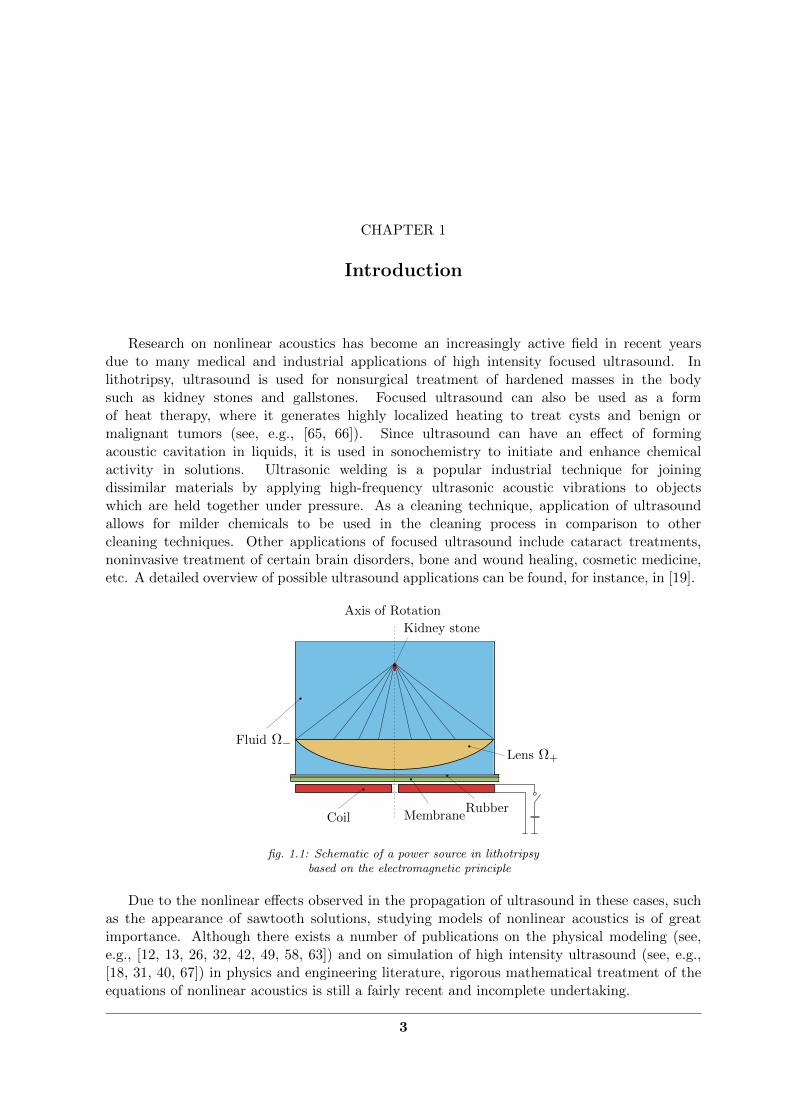
Research on nonlinear acoustics has become an increasingly active field in recent yearsdue to many medical and industrial applications of high intensity focused ultrasound. Inlithotripsy, ultrasound is used for nonsurgical treatment of hardened masses in the bodysuch as kidney stones and gallstones. Focused ultrasound can also be used as a formof heat therapy, where it generates highly localized heating to treat cysts and benign ormalignant tumors (see, e.g., [65, 66]). Since ultrasound can have an effect of formingacoustic cavitation in liquids, it is used in sonochemistry to initiate and enhance chemicalactivity in solutions. Ultrasonic welding is a popular industrial technique for joiningdissimilar materials by applying high-frequency ultrasonic acoustic vibrations to objectswhich are held together under pressure. As a cleaning technique, application of ultrasoundallows for milder chemicals to be used in the cleaning process in comparison to othercleaning techniques. Other applications of focused ultrasound include cataract treatments,noninvasive treatment of certain brain disorders, bone and wound healing, cosmetic medicine,etc. A detailed overview of possible ultrasound applications can be found, for instance, in [19].

Coil MembraneRubber

Kidney stone

Axis of Rotation

Lens Ω+

Fluid Ω−

fig. 1.1: Schematic of a power source in lithotripsybased on the electromagnetic principle

Due to the nonlinear effects observed in the propagation of ultrasound in these cases, suchas the appearance of sawtooth solutions, studying models of nonlinear acoustics is of greatimportance. Although there exists a number of publications on the physical modeling (see,e.g., [12, 13, 26, 32, 42, 49, 58, 63]) and on simulation of high intensity ultrasound (see, e.g.,[18, 31, 40, 67]) in physics and engineering literature, rigorous mathematical treatment of theequations of nonlinear acoustics is still a fairly recent and incomplete undertaking.

3

Chapter 1. Introduction

The work in this thesis is motivated, e.g., by lithotripsy, where mathematical analysis,numerical simulation, and optimization are expected to lead to a better understanding andcontrol of the physical effects and thus to a substantial reduction of lesions and a decrease incomplication risks during treatment.

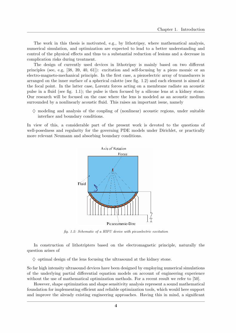
The design of currently used devices in lithotripsy is mainly based on two differentprinciples (see, e.g, [38, 39, 40, 61]): excitation and self-focusing by a piezo mozaic or anelectro-magneto-mechanical principle. In the first case, a piezoelectric array of transducers isarranged on the inner surface of a spherical calotte (see fig. 1.2) and each element is aimed atthe focal point. In the latter case, Lorentz forces acting on a membrane radiate an acousticpulse in a fluid (see fig. 1.1); the pulse is then focused by a silicone lens at a kidney stone.Our research will be focused on the case where the lens is modeled as an acoustic mediumsurrounded by a nonlinearly acoustic fluid. This raises an important issue, namely

♦ modeling and analysis of the coupling of (nonlinear) acoustic regions, under suitableinterface and boundary conditions.

In view of this, a considerable part of the present work is devoted to the questions ofwell-posedness and regularity for the governing PDE models under Dirichlet, or practicallymore relevant Neumann and absorbing boundary conditions.

fig. 1.2: Schematic of a HIFU device with piezoelectric excitation

In construction of lithotripters based on the electromagnetic principle, naturally thequestion arises of

♦ optimal design of the lens focusing the ultrasound at the kidney stone.

So far high intensity ultrasound devices have been designed by employing numerical simulationsof the underlying partial differential equation models on account of engineering experiencewithout the use of mathematical optimization methods. For a recent result we refer to [50].

However, shape optimization and shape sensitivity analysis represent a sound mathematicalfoundation for implementing efficient and reliable optimization tools, which would here supportand improve the already existing engineering approaches. Having this in mind, a significant

4

part of the present work is dedicated to the mathematically rigorous derivation of first ordersensitivities in the context of the respective governing PDE model, which will serve as a basisfor developing an effective optimization algorithm.

Contents of the chapters

Chapter 2 introduces the most popular model in nonlinear acoustics - Westervelt’sequation, as well as the model we will be working with which has an added strong nonlineardamping term of q-Laplace type. We will present the governing equations and lay out theinherent difficulties of working with this model.

Chapter 3 contains an overview of certain well-known theoretical results concerningSobolev spaces and ODE existence theory as well as a number of helpful inequalities, whichare all often employed in the rest of the thesis.

Chapter 4 is dedicated to the question of well-posedness for the Westervelt equation withstrong nonlinear damping. Unlike [9], we investigate this model under Neumann as well asabsorbing boundary conditions. Additionally, advantages of introducing lower order linear andnonlinear damping terms are investigated. Moreover, well-posedness in case of acoustic-acousticcoupling, as relevant in devices following schematic from figure 1.1, is shown. The resultspresented here are based on the following work:

V. Nikolic, Local existence results for the Westervelt equation with nonlinear damping andNeumann as well as absorbing boundary conditions, Journal of Mathematical Analysisand Applications, vol. 427, issue 2, 1131–1167, 2015.

Chapter 5 deals with the question of higher interior regularity for the Westervelt equationwith strong nonlinear damping as well as for the system of these models coupled throughinterface conditions. Regularity up to the boundary/interface is also obtained under theassumption that the gradient of the acoustic pressure stays essentially bounded in time andspace; this represents the foundation for the shape sensitivity analysis in the next chapter.Chapter 5 is based on the following work:

V. Nikolic and B. Kaltenbacher, On higher regularity for the Westervelt equation withstrong nonlinear damping, arXiv:1506.02125 [math.AP], and submitted.

Chapter 6 provides shape sensitivity analysis for the problem of finding the optimal shapeof a focusing lens in lithotripsy (cf. fig. 1.1) and gives an answer to the question of existence ofsuch optimal shapes. Shape derivative is obtained through a variational approach introducedby Ito, Kunisch and Peichl in [30], which does not require shape differentiability of the statevariable. This chapter relies on the following result:

V. Nikolic and B. Kaltenbacher, Sensitivity analysis for shape optimization of a focusingacoustic lens in lithotripsy, arXiv:1506.02781 [math.AP], and submitted.

Comment on the notation. Throughout the thesis, we will employ the dot notation fordifferentiation (also known as Newton’s notation) with respect to the time variable, i.e. u andu will denote the first and the second time derivative of a function u.

5

Chapter 1. Introduction

6

CHAPTER 2

Westervelt’s equation

In this chapter, we will present the most commonly used mathematical model in nonlinearacoustics - Westervelt’s equation. It is named after the American physicist Peter Westervelt(1919–2015), renowned for, among other things, introducing the concept of the parametricarray in [63]. Westervelt’s equation originated as a by-product of this discovery.

2.1 Governing equations

The propagation of waves is described by the following quantities (see, for example, [39,Chapter 5]):

time and spatial variation of the density %∼ = massvolume [kg/m3],

pressure u∼ = forcecross section [N/m2],

velocity v∼ = distancetime [m/s].

These quantities can be decomposed into their mean (whose time and - in case of homogeneousfluids - also space derivatives vanish) and alternating part as follows:

%∼ = %0 + %, u∼ = u0 + u, v∼ = v0 + v.

Here % denotes the acoustic density and u the acoustic pressure, and v is the acoustic particlevelocity. For the derivation of the Westervelt equation, zero mean velocity is assumed, i.e.v∼ = v. The acoustic field in a fluid can be fully described by the following equations:

Navier-Stokes equation for momentum conservation:

%(v + (v · ∇)v) +∇u = µV ∆v + (µV3

+ ηV )∇(∇ · v),

here µV denotes the shear viscosity and ηV the bulk viscosity; under the assumption that∇× v = 0 the equation reduces to

%(v + (v · ∇)v) +∇u = (4µV

3+ ηV )∆v;

the equation of continuity (conservation of mass):

∇ · (%v) = −%;

7

Chapter 2. Westervelt’s equation

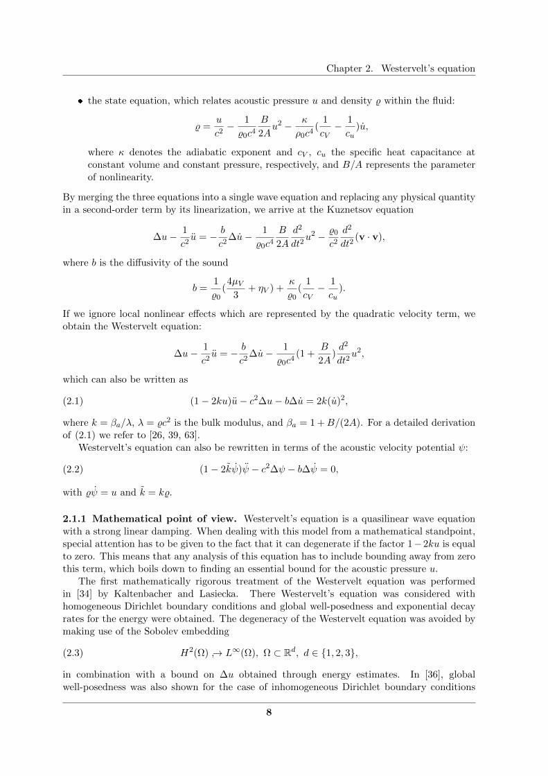
the state equation, which relates acoustic pressure u and density % within the fluid:

% =u

c2− 1

%0c4

B

2Au2 − κ

ρ0c4(

1

cV− 1

cu)u,

where κ denotes the adiabatic exponent and cV , cu the specific heat capacitance atconstant volume and constant pressure, respectively, and B/A represents the parameterof nonlinearity.

By merging the three equations into a single wave equation and replacing any physical quantityin a second-order term by its linearization, we arrive at the Kuznetsov equation

∆u− 1

c2u = − b

c2∆u− 1

%0c4

B

2A

d2

dt2u2 − %0

c2

d2

dt2(v · v),

where b is the diffusivity of the sound

b =1

%0(4µV

3+ ηV ) +

κ

%0(

1

cV− 1

cu).

If we ignore local nonlinear effects which are represented by the quadratic velocity term, weobtain the Westervelt equation:

∆u− 1

c2u = − b

c2∆u− 1

%0c4(1 +

B

2A)d2

dt2u2,

which can also be written as

(1− 2ku)u− c2∆u− b∆u = 2k(u)2,(2.1)

where k = βa/λ, λ = %c2 is the bulk modulus, and βa = 1 +B/(2A). For a detailed derivationof (2.1) we refer to [26, 39, 63].

Westervelt’s equation can also be rewritten in terms of the acoustic velocity potential ψ:

(1− 2kψ)ψ − c2∆ψ − b∆ψ = 0,(2.2)

with %ψ = u and k = k%.

2.1.1 Mathematical point of view. Westervelt’s equation is a quasilinear wave equationwith a strong linear damping. When dealing with this model from a mathematical standpoint,special attention has to be given to the fact that it can degenerate if the factor 1−2ku is equalto zero. This means that any analysis of this equation has to include bounding away from zerothis term, which boils down to finding an essential bound for the acoustic pressure u.

The first mathematically rigorous treatment of the Westervelt equation was performedin [34] by Kaltenbacher and Lasiecka. There Westervelt’s equation was considered withhomogeneous Dirichlet boundary conditions and global well-posedness and exponential decayrates for the energy were obtained. The degeneracy of the Westervelt equation was avoided bymaking use of the Sobolev embedding

H2(Ω) → L∞(Ω), Ω ⊂ Rd, d ∈ 1, 2, 3,(2.3)

in combination with a bound on ∆u obtained through energy estimates. In [36], globalwell-posedness was also shown for the case of inhomogeneous Dirichlet boundary conditions

8

2.2. Westervelt’s equation with strong nonlinear damping

and in [35] the results were extended to the Neumann problem for the Westervelt equation; inboth cases the equation was kept away from degenerating by employing (2.3).

Due to this need to steer clear of degeneracy, for the Westervelt equation only solutionswhich are very smooth, i.e. H2-regular in space, can be shown to exist. However, since oneof our central tasks is to study the interface coupling of acoustic regions, which is a commonoccurrence in applications, achieving this regularity over the whole domain will be too high ofa demand. As we will see, these acoustic regions will possess different material parameters andthe normal derivative of the acoustic pressure will jump over the joint interface, thus makingH2-regularity of the acoustic pressure over the whole domain impossible.

2.2 Westervelt’s equation with strong nonlinear damping

As a way of relaxing regularity of solutions, and having acoustic-acoustic coupling in mind,Westervelt’s equation is considered with an added strong nonlinear damping term:

(2.4) (1− 2ku)u− c2∆u− div(b((1− δ) + δ|∇u|q−1)∇u) = 2k(u)2

with δ ∈ (0, 1), q ≥ 1, q > d − 1, d ∈ 1, 2, 3. For this model, which was first introduced in[9], degeneracy can be avoided by the means of the embedding

W 1,q+1(Ω) → L∞(Ω), Ω ⊂ Rd, d ∈ 1, 2, 3, q > d− 1,

in combination with a bound on |u(t)|W 1,q+1(Ω), which can be obtained through energyestimates. Using this model therefore allows to show existence of W 1,q+1-regular in spaceweak solutions, and in turn well-posedness of the acoustic-acoustic coupling problem.

Introduction of the q-Laplace term to the Westervelt equation is, on the other hand,motivated by models for power-law fluids (see, e.g., [62]), where the effective viscosity isproportional to certain power of the shear rate, which is used in the relation

shear stress = shear rate times effective viscosity.

The shear rate is always a spatial derivative of the velocity, which in its turn (via the linearizedversion of the Navier-Stokes equation) can be rewritten in terms of the pressure gradient. Thisis a physical motivation behind the appearance of the gradient of pressure under the q-powerin the model.

2.2.1 q-Laplacian. In comparison to (2.1), equation (2.4) has a new important feature,namely a damping term obtained by applying the q-Laplace operator

∆qu := −div(|∇u|q−1∇u),(2.5)

q ≥ 1, to the first time derivative of u:

∆qu := −div(|∇u|q−1∇u).

In the special case of q = 1, (2.5) reduces to the standard Laplacian.Working with the new model (2.4) implies handling this q-Laplace damping term in terms

of analysis, numerics and optimization, which is a nontrivial task. The q-Laplace equation,given by

−∆qu = f,(2.6)

9


and the parabolic q-Laplace equation

u−∆qu = f,(2.7)

where f belongs to an appropriate function space, have been extensively studied in the pastwith respect to regularity (see, for example, [46, 60, 16, 21] and references given therein) andnumerical treatment (see, for instance, [17, 6, 47, 7]).

Regarding shape optimization problems which are governed by q-Laplace type equations,the few existing results seem to trace back to [10], where the continuity of the solution to aDirichlet problem was considered with respect to domain perturbations. For a recent account,we refer to [11], where the optimal placement of a Dirichlet region in a domain, governedby (2.6), was studied. However, investigations on the interface coupling of q-Laplace typeequations, in terms of numerics and optimization, seem to be lacking in the mathematicalliterature.

Results on hyperbolic equations with damping of q-Laplace type are sparse and so far havebeen mostly concerned with local and global well-posedness. In [64, 54] a wave equation witha q-Laplace damping and a nonlinear source was considered and global well-posedness wasshown. Global existence and asymptotic behavior were achieved in [25] for a nonlinear waveequation with a q-Laplace damping term. However, other features of (2.4), such as the potentialdegeneracy, were not present in [25] and [64, 54].

In [9], equation (2.4) was investigated for the first time, under homogeneous Dirichletboundary conditions and local in time well-posedness was obtained, as well as the short timewell-posedness for an interface coupling of these models under homogeneous Dirichlet boundaryconditions on the outer boundary.

A shape optimization problem governed by the Westervelt equation (2.1) was recentlyconsidered in [37]; however, there are seemingly no considerations in literature of shapeoptimization problems governed by hyperbolic equations with q-Laplace damping terms orcoupled systems of these types of models (save for our work in [53] which will be presentedhere).

2.2.2 Different nonlinear damping terms. In [9, 51], the possibility of adding differentnonlinear damping terms to the Westervelt equation (2.1) was also investigated, namely addinga q-Laplace damping term

(1− 2ku)u− c2∆u− div(b((1− δ) + δ|∇u|q−1)∇u) = 2k(u)2,(2.8)

as well as

ψ − c2

1− 2kψ∆u− bdiv(((1− δ) + δ|∇ψ|q−1)∇ψ) = 0;(2.9)

the second model is motivated by the acoustic velocity potential formulation (2.2). However, forthese models only local existence of solutions could be shown, but not well-posedness, mainlybecause it was not possible to obtain higher order energy estimates. In this way, model (2.4)turned out to be the most ”well-behaved”. For more details on (2.8) and (2.9), we refer to [9,Section 3 and 6] and [51, Section 4 and 5].

2.3 Interface coupling in nonlinear acoustics

Coupling of acoustic regions over a joint interface is an important occurrence in highintensity focused ultrasound applications, e.g. in lithotripsy, where an acoustic lens, which

10

2.3. Interface coupling in nonlinear acoustics

focuses the ultrasound, is immersed in an acoustic fluid medium (see fig. 1.1). Naturally, thequestion of modeling and well-posedness in this context arises.

The case of the acoustic-acoustic coupling can be modeled by the presence of spatiallyvarying coefficients, with possible jumps over interfaces between subdomains, in the weak formof the equation (2.4) (see [5] for the linear, and [9] and [51] for the nonlinear case):

(2.10)

Find u such that∫ T0

∫Ω

1λ(x)(1− 2k(x)u)uφ+ 1

%(x)∇u · ∇φ+ b(x)(1− δ(x))∇u · ∇φ

+b(x)δ(x)|∇u|q−1∇u · ∇φ− 2k(x)λ(x) (u)2φ dx ds = 0

holds for all test functions φ ∈ X,

with (u, u)|t=0 = (u0, u1), and appropriately chosen test space X (which will be specified in theforthcoming chapters together with assumptions on the coefficients). In this model b denotesthe quotient between the diffusivity and the bulk modulus, while other coefficients retain theirmeaning. For notational brevity, we emphasized the space dependence of coefficients in (2.10),while omitting space and time dependence of u and the test function in the notation.

In the next chapter, we will tackle the question of local in time well-posedness for thismodel, and later on it will also appear as a governing model when optimizing the shape of thefocusing lens.

We also briefly mention that the focusing lens in lithotripsy can be modeled as an elasticmedium, which leads to the problem of an elastic-acoustic coupling. This more advanced model,was considered in [9]:

%(x)ψ − BT 1

1− 2k(x)φ[c](x)Bψ + BT

(((1− δ(x)) + δ(x)|Bψ|q−1)[b](x)Bψ

)= 0,(2.11)

under homogeneous Dirichlet boundary conditions and suitable assumptions on the spatiallyvarying coefficients. Here ψ denotes the acoustic velocity potential, φ stands for the gradientpart in the Helmholtz decomposition of ψ, ψ = ∇φ +∇ ×A , and the first order differentialoperator B is given by

B =

∂x1 0 0 0 ∂x3 ∂x2

0 ∂x2 0 ∂x3 0 ∂x1

0 0 ∂x3 ∂x2 ∂x1 0

T

.

For this model local in time well-posedness was obtained in [9] under Dirichlet boundaryconditions.

11


12

CHAPTER 3

Theoretical preliminaries

In this chapter, we will collect certain well-known theoretical results which will be oftenemployed throughout the rest of the thesis as well as a number of helpful inequalities.

3.1 Sets of classes C l and C l,1

Going forward, we will be working with either Lipschitz domains or at several instancesC1,1-regular domains. We recall their definition here:

Definition 3.1. [[23], Definition 1.2.1.1] Let l,m ∈ N, 1 ≤ l,m ≤ ∞ and let Ω be an opensubset of Rd. We say that its boundary Γ is continuous (respectively Lipschitz, continuouslydifferentiable, of class C l,1, m times continuously differentiable) if for every x ∈ Γ there existsa neighborhood U of x in Rd and new orthogonal coordinates (y1, . . . , yd) such that

(i) U is a hypercube in the new coordinates:

U = (y1, . . . , yd) : −aj < yj < aj , 1 ≤ j ≤ d;

(ii) there exists a continuous (respectively Lipschitz, continuously differentiable, of class C l,1,m times continuously differentiable) function ϕ, defined in

U ′ = (y1, . . . , yd−1) : −aj < yj < aj , 1 ≤ j ≤ d− 1,

and such that

|ϕ(y′)| ≤ ad2, for every y′ = (y1, . . . , yd−1) ∈ U ′,

Ω ∩ U = y = (y′, yd) ∈ U : yd < ϕ(y′),Γ ∩ U = y = (y′, yd) ∈ U : yd = ϕ(y′).

A C l,1-mapping with a C l,1-inverse is called a C l,1-diffeomorphism.

Theorem 3.2. [[14], Theorem 2.6] Let Ω be a Lipschitzian domain in Rd. Then for all integersl ≥ 0, W l+1,∞(Ω) = C l,1(Ω) algebraically and topologically.

3.2 Sobolev embeddings

In the remaining of the thesis, we will employ a number of Sobolev embeddings, which wefor that reason recall here. For a thorough introduction and results on Sobolev spaces we referthe reader to [1].

13

Chapter 3. Theoretical preliminaries

Definition 3.3. [[4], Definition 7.3.6] Let X and Y be two Banach spaces over the domain Ωwith X ⊂ Y . We say that the space X is continuously embedded in Y and write X → Y if

‖u‖X ≤ CΩX,Y ‖u‖Y , ∀u ∈ X.(3.1)

The space X is compactly embedded in Y , denoted X →→ Y , if (3.1) holds and each boundedsequence in X has a convergent subsequence in Y .

Theorem 3.4. [[4], Theorem 7.3.7] Let Ω ⊂ Rd be a Lipschitz domain. The followingcontinuous embeddings hold:

if l < dr , then W l,r(Ω) → Lq(Ω) for any q ≤ r?, 1

r? = 1r −

ld ,

if l = dr , then W l,r(Ω) → Lq(Ω) for any q <∞,

if l > dr , then W l,r(Ω) → C l−[ d

r]−1,β(Ω), where

β =

[dr ] + 1− d

r , if dr 6= integer,

any positive number < 1, if dr = integer.

Theorem 3.5. [[4], Theorem 7.3.8] Let Ω ⊂ Rd be a Lipschitz domain. The following compactembeddings hold:

if l < dr , then W l,r(Ω) →→ Lq(Ω) for any q < r?, 1

r? = 1r −

ld ,

if l = dr , then W l,r(Ω) →→ Lq(Ω) for any q <∞,

if l > dr , then W l,r(Ω) →→ C l−[ d

r]−1,β(Ω), where β ∈ [0, [dr ] + 1− d

r ).

In particular, the following embeddings hold and will be often employed throughout the thesis:

H1(Ω) →→ L4(Ω), with the norm CΩH1,L4 ,(3.2)

Lr(Ω) → Lq(Ω), r ≥ q, with the norm CΩLr,Lq ,(3.3)

W 1,q+1(Ω) → L∞(Ω), q > d− 1, with the norm CΩW 1,q+1,L∞ .(3.4)

3.3 Traces

We also briefly recall the results on the density of smooth functions, as well as the conceptof traces in Sobolev spaces. For an in-depth survey of this topic, we refer to [1] and [44].

Theorem 3.6. (Meyers-Serin, [[44], Theorem 10.15]) Let Ω ⊂ Rd be an open set and let 1 ≤r <∞. Then the space C∞(Ω) ∩W 1,r(Ω) is dense in W 1,r(Ω).

Note that the Meyers-Serrin theorem does not hold for functions in W 1,∞(Ω).

Theorem 3.7. [[23], Theorem 1.5.1.3] Let Ω be a bounded open subset of Rd with a Lipschitzboundary Γ. Then the mapping

u 7→ u|Γ,

which is defined for u ∈ C(Ω), has a unique continuous extension as an operator from W 1,r(Ω)

onto W 1− 1r,r(Γ), 1 < r < ∞. This operator has a right continuous inverse which does not

depend on r.

14

3.4. Fundamental theorems

The extended operator is called the trace operator and will be in future denoted by trΓ.

Theorem 3.8. [[23], Theorem 1.5.1.2] Let Ω be a bounded open subset of Rd with a C1,1

boundary Γ. Assume that l− 1r is not an integer, 1 < r <∞, l ≤ 2, l− 1

r = l0 + σ, 0 < σ < 1,and l0 is a nonnegative integer. Then the mapping

u 7→ ∂u

∂n|Γ,

which is defined for u ∈ C1(Ω), has a unique continuous extension as an operator from W l,r(Ω)

onto W l−1− 1r,r(Γ). This operator has a right continuous inverse which does not depend on r.

Theorem 3.9. [[15], Theorem 3.42]) Let Ω be a class C1 open set and let u ∈W 1,r(Ω). Thenthere exists a sequence un ⊂ C∞(Ω) ∩W 1,r(Ω) that converges to u in W 1,r(Ω) and satisfiestrΓun = trΓu.

3.4 Fundamental theorems

Let us collect here three fundamental theorems which we will reference in the forthcomingchapters.

Theorem 3.10. (Dominated convergence theorem, [[20], Theorem 4, Appendix E]) Assumethe functions fm∞m=1 are integrable and fm → f a.e. Suppose also that |fm| ≤ g a.e. forsome summable function g. Then ∫

Rdfm dx→

∫Rdf dx.

Theorem 3.11. (Banach’s fixed-point theorem, [[55], Theorem 1.12]) A contractive mappingT : X → X on a Banach space X has a unique fixed point u, i.e. T (u) = u.

Theorem 3.12. (Bolzano-Weierstrass, [[55], Theorem 1.8]) Every lower (respectively upper)semicontinuous function X → R on a compact set attains its minimum (respectively maximum)on this set.

3.5 A local existence result for ordinary differential equations

As an auxiliary problem in Chapter 4, we will encounter an initial-value problem of thefollowing type:

(3.5)u = f(t, u(t)) for a.e. t ∈ [0, T ]

u(0) = u0,

where the right hand side f : (0,+∞)× Rk → Rk will be a Caratheodory mapping:

Definition 3.13. [[55], Chapter 1] Considering integers j,m0, . . . ,mj we say that a mappinga : (0, T )×Rm1× . . .×Rmj → Rm0 is a Caratheodory mapping if a(·, r1, . . . , rj) : (0, T )→ Rm0

is measurable for all (r1, . . . , rj) ∈ Rm1 × . . . × Rmj and a(t, ·) : Rm1 × . . . × Rmj → Rm0 iscontinuous for a.e. t ∈ (0, T ).

By solution on a time interval [0, T ] of (3.5) we will call an absolutely continuous mappingu : [0, T ]→ Rk such that the equation in (3.5) holds a.e. on [0, T ] and u(0) = u0. The followingshort-time existence result holds:

15


Theorem 3.14. [[55], Theorem 1.44] Let f : (0,+∞)× Rk → Rk be a Caratheodory mapping.Then there exists T > 0 such that the initial-value problem (3.5) has a solution on the interval[0, T ].

3.6 Helpful inequalities

Finally, we gather here essential inequalities which we will rely upon throughout the restof the thesis.

In the case of problems with inhomogeneous Neumann boundary data it is often necessaryto employ Poincare’s inequality valid for functions in W 1,q+1(Ω). We recall such inequality(see, e.g., [44, Theorem 12.23]), namely that there exists a constant CP > 0 depending on qand Ω such that

|ϕ− 1

|Ω|

∫Ωϕdx|Lq+1(Ω) ≤ CP |∇ϕ|Lq+1(Ω),(3.6)

for all ϕ ∈W 1,q+1(Ω).Throughout the thesis, we will assume that t ∈ [0, T ], where T is a finite time horizon.

From (3.6) we can obtain

|u(t)|W 1,q+1(Ω) ≤ (1 + CP )|∇u(t)|Lq+1(Ω) + CΩ1

∣∣∣ ∫Ωu(t) dx

∣∣∣,(3.7)

and by replacing u with u also

|u(t)|W 1,q+1(Ω) ≤ (1 + CP )|∇u(t)|Lq+1(Ω) + CΩ2 |u(t)|L2(Ω),(3.8)

a.e. in time, where CΩ1 = |Ω|−

qq+1 and CΩ

2 = |Ω|−q−1

2(q+1) . By employing the embedding (3.4)and estimate (3.7), we can as well obtain

|u(t)|L∞(Ω) ≤CΩW 1,q+1,L∞ |u(t)|W 1,q+1(Ω)

≤CΩW 1,q+1,L∞

[(1 + CP )|∇u(t)|Lq+1(Ω) + CΩ

1

∣∣∣ ∫Ωu(t) dx

∣∣∣]≤CΩ

W 1,q+1,L∞

[(1 + CP )|∇u0 +

∫ t

0∇u(s) ds|Lq+1(Ω) + CΩ

1 |u0|L1(Ω)

+ CΩ2

∫ t

0|u(t)|L2(Ω) ds

]≤CΩ

W 1,q+1,L∞

[(1 + CP )(|∇u0|Lq+1(Ω) + (tq

∫ t

0|∇u|q+1

Lq+1(Ω)ds)1/q+1)

+ CΩ1 |u0|L1(Ω) + CΩ

2

∫ t

0|u(t)|L2(Ω) ds

],

which leads to the estimate

‖u‖L∞(0,T ;L∞(Ω)) ≤CΩW 1,q+1,L∞

[(1 + CP )(|∇u0|Lq+1(Ω) + T

qq+1 ‖∇u‖Lq+1(0,T ;Lq+1(Ω)))

+ CΩ1 |u0|L1(Ω) + CΩ

2 T‖u‖L∞(0,T ;L2(Ω))

],

(3.9)

that will be employed when dealing with the possible degeneracy of the factor 1 − 2ku. Toobtain these estimates, we have assumed that u is sufficiently regular in time and space so that

16

3.6. Helpful inequalities

the right hand sides make sense.We will also frequently make use of Young’s inequality in the ε-form

xy ≤ εxr + C(ε, r)yrr−1 (x, y > 0, ε > 0, 1 < r <∞),(3.10)

with C(ε, r) = (r − 1)rrr−1 ε−

11−r .

3.6.1 Inequalities involving q-Laplacian. Let us also recall several useful inequalities thatwe will need when handling the q-Laplace damping term. They can be found in [46, Chapter10] and [47, Appendix]. From now on, Cq will be used to denote a generic constant dependingonly on q. For any x, y ∈ Rd and η ≥ 0 it holds

||x|q−1x− |y|q−1y| ≤ Cq|x− y|1−η(|x|+ |y|)q−1+η, q > 0,(3.11)

(3.12)(|x|q−1x− |y|q−1y) · (x− y) ≥ 2−1|x− y|2(|x|q−1 + |y|q−1)

≥ 21−q|x− y|q+1 ≥ 0, q ≥ 1,

4

(q + 1)2||x|

q−12 x− |y|

q−12 y|2 ≤ (|x|q−1x− |y|q−1y) · (x− y), q ≥ 1,(3.13)

||x|q−1x− |y|q−1y| ≤ q(|x|q−1

2 + |y|q−1

2 )||x|q−1

2 x− |y|q−1

2 y|, q ≥ 1.(3.14)

From (3.11) we also get

||x|q − |y|q| ≤ Cq |x− y|1−η(|y|q−1+η + |x|q−1+η),(3.15)

for 0 ≤ η ≤ 1, q > 1.In several instances, we will utilize the following representation formula for vectors x, y ∈ Rd(cf. [46, Chapter 10]):

(3.16)

|x|q−1x− |y|q−1y

= (x− y)

∫ 1

0|y + σ(x− y)|q−1 dσ + (q − 1)

∫ 1

0L(y + σ(x− y), (x− y) dσ,

where

(3.17) L(x, y) = |x|q−3(x · y)x

as well as the inequality

|y + σ(x− y)|q−1 ≤ |y|q−1 + |x|q−1, σ ∈ [0, 1].(3.18)

With the notation (3.17), as a simple consequence of (3.11), we have for vectors x, y, z, w andany η ≥ 0, q > 2 that

(3.19)

|L(x, y)− L(z, w)|= |(x · y)(|x|q−3x− |z|q−3z) + |z|q−3((y − w) · x+ w · (x− z))z|≤Cq|x− z|1−η(|x|q−3+η + |z|q−3+η)|x||y|+ |z|q−2(|y − w||x|+ |w||x− z|).

17


18

CHAPTER 4

Local well-posedness results for the Westervelt equation withnonlinear damping

In this chapter, we will investigate the Westervelt equation with strong nonlinear damping(2.4), under practically relevant absorbing and Neumann boundary conditions. Our researchinto this area is motivated by many applications of high intensity focused ultrasound wherethe need for realistic boundary conditions is evident. Typically in acoustics one faces theproblem of a physically unbounded domain which should then be truncated for numericalcomputations. Absorbing boundary conditions are used as a way of avoiding reflections on theartificial boundary Γ of the computational domain. Ultrasound excitation, e.g. by piezoelectrictransducers (see fig. 1.2), can be modeled by Neumann boundary conditions on the rest of theboundary Γ = ∂Ω \ Γ. At the end of this chapter we will also consider the acoustic-acousticcoupling arising when focusing is done by an acoustic lens immersed in a fluid, cf. fig. 1.1.

4.1 Dirichlet boundary conditions

Before we proceed to the case of Neumann and absorbing boundary conditions, let usrecall the local well-posedness result for the Dirichlet problem, obtained by Brunnhuber,Kaltenbacher, and Radu in [9]. We assume Ω ⊂ Rd, d ∈ 1, 2, 3 to be an open, connected,bounded set with Lipschitz boundary and consider the following problem:

(1− 2ku)u− c2∆u− bdiv (((1− δ) + δ|∇u|q−1)∇u) = 2k(u)2 in Ω× (0, T ],

u = 0 on ∂Ω× (0, T ],

(u, u) = (u0, u1) on Ω× t = 0,

(4.1)

with the following assumptions on the coefficients and the exponent q:

c2, b > 0, δ ∈ (0, 1), k ∈ R, q > d− 1, q ≥ 1.(4.2)

The weak formulation reads as

(4.3)

∫ T

0

∫Ω(1− 2ku)uφ+ c2∇u · ∇φ+ b(1− δ)∇u · ∇φ

+bδ|∇u|q−1∇u · ∇φ− 2k(u)2φ dx ds = 0

holds for all test functions φ ∈ X = L2(0, T ;W 1,q+10 (Ω)),

with (u, u) = (u0, u1). The following well-posedness result holds:

19

Chapter 4. Local well-posedness results

Proposition 4.1. [[9], Theorem 2.3] Let assumptions (4.2) hold. For any T > 0 there is aκT > 0 such that for all u0, u1 ∈W 1,q+1

0 (Ω) with

|u1|2L2(Ω) + |∇u0|2L2(Ω) + |∇u1|2L2(Ω) + |∇u1|q+1Lq+1(Ω)

+ |∇u0|2Lq+1(Ω) ≤ κ2T ,

there exists a weak solution u ∈ W ⊂ X = H2(0, T ;L2(Ω)) ∩W 1,∞(0, T ;W 1,q+10 (Ω)) of (4.1),

and

W = v ∈ X : ‖v‖L2(0,T ;L2(Ω)) ≤ m ∧ ‖∇v‖L∞(0,T ;L2(Ω)) ≤ m∧‖∇v‖Lq+1(0,T ;Lq+1(Ω)) ≤ M ∧ (v, v) = (u0, u1),

with2|k|CΩ

W 1,q+10 ,L∞

(κT + Tqq+1 M) < 1,

and m sufficiently small, and u is unique in W.

In [9], the issue of possible degeneracy of the Westervelt equation due to the factor 1− 2kuis resolved by the means of the embedding W 1,q+1

0 (Ω) → L∞(Ω), valid for q > d− 1, and thefollowing estimate

|u(x, t)| ≤CΩW 1,q+1

0 ,L∞|∇u(t)|Lq+1(Ω)

≤CΩW 1,q+1

0 ,L∞|∇u0 +

∫ t

0∇u ds |Lq+1(Ω)

≤CΩW 1,q+1

0 ,L∞

(|∇u0|Lq+1(Ω) +

(tq∫ t

0

∫Ω|∇u(y, s)|q+1 dy ds

) 1q+1),

which leads to the bound

(4.4)1− a0 < 1− 2ku < 1 + a0,

a0 := 2|k|CΩW 1,q+1

0 ,L∞(|∇u0|Lq+1(Ω) + T

qq+1 ‖∇u‖Lq+1(0,T ;Lq+1(Ω))).

Due to the embedding W 1,q+1(Ω) → C0,1− d

q+1 (Ω), we also know that u is Holder continuous

in space, i.e. u ∈ C0,1(0, T ;C0,1− d

q+1 (Ω)).

4.2 Neumann as well as absorbing boundary conditions

In this section ∂Ω is assumed to be a disjoint union of Γ and Γ. We denote by n the outwardunit normal vector. In our case, the design of the nonlinear absorbing and inhomogeneousNeumann boundary conditions is influenced by the presence of the nonlinear strong dampingin the equation (2.4). We will study initial boundary value problems of the following type:

(1− 2ku)u− c2∆u− bdiv(((1− δ) + δ|∇u|q−1)∇u) + βu

= 2k(u)2 in Ω× (0, T ],

c2 ∂u∂n + b((1− δ) + δ|∇u|q−1)∂u∂n = g on Γ× (0, T ],

αu+ c2 ∂u∂n + b((1− δ) + δ|∇u|q−1)∂u∂n = 0 on Γ× (0, T ],

(u, u) = (u0, u1) on Ω× t = 0,

(4.5)

20

4.2. Neumann as well as absorbing boundary conditions

(1− 2ku)u− c2∆u− bdiv(((1− δ) + δ|∇u|q−1)∇u) + γ|u|q−1u

= 2k(u)2 in Ω× (0, T ],



(u, u) = (u0, u1) on Ω× t = 0.

(4.6)

Compared to the Westervelt equation with strong nonlinear damping (2.4) we havediscussed so far, these equations have additional lower order damping terms. We assume thatparameters β and γ are nonnegative; the case β = γ = 0 reduces them back to (2.4). We willin this way also look into the possible introduction of these lower order linear and nonlineardamping terms to equation (2.4), this becomes beneficial when deriving energy estimates.

The additional difficulty as compared to the Dirichlet case lies in not being able to usePoincare’s inequality for functions in W 1,q+1

0 (Ω), therefore we always have to find appropriateestimates of the zero order space derivative terms of u to be combined with the first orderones and employed in the trace estimates of the g terms arising from multiplication with uand u. As a matter of fact, we will try to tune these combinations to minimize the restrictionson T and on the norms of the data. This will lead to different combinations in the casesβ = γ = 0 (Propositions 4.3, 4.6, Theorem 4.10), β > 0 (Proposition 4.7, Theorem 4.12), γ > 0(Proposition 4.8, Theorem 4.13).

Our results will hold for α assumed to be nonnegative, and they remain valid also in caseΓ = ∅, that is to say, with Neumann boundary conditions on the whole boundary. Note thatin the case of b = 0 and α = c the absorbing conditions prescribed in (4.5) and (4.6) wouldreduce to the standard linear absorbing boundary conditions of the form u+ c∂u∂n = 0.

In what is to follow, we will denote by Ctr1 the norm of the trace mapping

trΓ : W 1,q+1(Ω)→W1− 1

q+1,q+1

(Γ),

and by Ctr2 the norm of the trace mapping trΓ : H1(Ω)→ H−1/2(Γ) (with Ctr1 = Ctr2 for q = 1).

We will begin by looking at problems (4.5) and (4.6) with β = γ = 0 (in other words, aninitial-boundary value problem for the equation (2.4)):

(1− 2ku)u− c2∆u− bdiv(((1− δ) + δ|∇u|q−1)∇u) = 2k(u)2 in Ω× (0, T ],



(u, u) = (u0, u1) on Ω× t = 0,

(4.7)

and then later on consider the addition of lower order damping terms.

4.2.1 Partially linearized model. Following the approach in [9], we will first consider apartially linearized version of the PDE in (4.7), where nonlinearity remains only in the damping

21


term:

(4.8)

au− c2∆u− bdiv(((1− δ) + δ|∇u|q−1)∇u) + fu = 0 in Ω× (0, T ]



(u, u) = (u0, u1) on Ω× t = 0,

and prove local well-posedness for this model first.

Definition 4.2. (Weak solution) Let a ∈ L∞(0, T ;L∞(Ω)), a ∈ L∞(0, T ;L2(Ω)), f ∈L∞(0, T ;L4(Ω)), u0 ∈ H1(Ω), u1 ∈ L2(Ω) and g ∈ L

q+1q (0, T ;W

− qq+1

, q+1q (Γ)). We say that

u ∈ v : v ∈ H1(0, T ;H1(Ω)) ∧ v ∈ Lq+1(0, T ;W 1,q+1(Ω))

is a weak solution of (4.8) if the following identity holds

−∫ T

0

∫Ωu(aw + aw) dx ds+

∫ T

0

∫Ω

c2∇u · ∇w + b((1− δ) + δ|∇u|q−1)∇u · ∇w

dx ds

+ α

∫ T

0

∫Γuw dx ds

= −∫ T

0

∫Ωfuw dx ds+

∫ T

0

∫Γgw dx ds−

∫Ωa(0)u1w(0) dx,

and u(0) = u0, for all w ∈ H1(0, T ;W 1,q+1(Ω)), w(T ) = 0.

Proposition 4.3. Let T > 0, c2, b > 0, α ≥ 0, δ ∈ (0, 1), q ≥ 1 and assume that

(i) a ∈ L∞(0, T ;L∞(Ω)), a ∈ L∞(0, T ;L2(Ω)), 0 < a ≤ a(x, t) ≤ a,

f ∈ L∞(0, T ;L4(Ω)),

g ∈ Lq+1q (0, T ;W

− qq+1

, q+1q (Γ)),

u0 ∈ H1(Ω), u1 ∈ L2(Ω),

with

‖f − 1

2a‖L∞(0,T ;L2(Ω)) ≤ b < min

b(1− δ)2(CΩ

H1,L4)2,

a

4T (CΩH1,L4)2

.(4.9)

Then (4.8) has a unique weak solution in the sense of Definition 4.2,

(4.10)u ∈ X := v : v ∈ H1(0, T ;H1(Ω)) ∩W 1,∞(0, T ;L2(Ω))

∧ v ∈ Lq+1(0, T ;W 1,q+1(Ω)),

and u satisfies the energy estimate

(4.11)

[a4− b(CΩ

H1,L4)2T − ε0]‖u‖2L∞(0,T ;L2(Ω)) +

c2

4‖∇u‖2L∞(0,T ;L2(Ω)) +

α

2‖u‖2

L2(0,T ;L2(Γ))

+[b(1− δ)

2− b(CΩ

H1,L4)2]‖∇u‖2L2(0,T ;L2(Ω)) +

[bδ2− ε1

]‖∇u‖q+1

Lq+1(0,T ;Lq+1(Ω))

≤ a2|u1|2L2(Ω) +

c2

2|∇u0|2L2(Ω) +

1

4ε0(Ctr1 C

Ω2 )2‖g‖2

L1(0,T ;W− qq+1 ,

q+1q (Γ))

+ C(ε1, q + 1)(Ctr1 (1 + CP ))q+1q ‖g‖

q+1q

Lq+1q (0,T ;W

− qq+1 ,

q+1q (Γ))

,

22


for some constants

(4.12) 0 < ε0 <a

4− b(CΩ

H1,L4)2T, 0 < ε1 <bδ

2,

and depends Holder continuously (in X) on the initial and boundary data. Moreover, if a is

time independent, then au ∈ Lq+1q (0, T ; (W 1,q+1(Ω))?).

Remark 4.4. In case Γ = ∅, estimate (4.11) and all forthcoming estimates hold with α set tozero.

Proof. Consider the problem of finding u such that

(4.13)

∫Ω

a(t)u(t)w + c2∇u(t) · ∇w + b((1− δ) + δ|∇u(t)|q−1)∇u(t) · ∇w

dx

+ α

∫Γu(t)w dx

= −∫

Ωf(t)u(t)w dx+

∫Γg(t)w dx, ∀w ∈W 1,q+1(Ω), a.e. t ∈ [0, T ],

with initial conditions (u0, u1).We will use the standard Faedo-Galerkin method (see for instance [20, Section 7.2] for the

case of second-order linear hyperbolic equations and [9, Section 2] for the problem (4.8) withhomogeneous Dirichlet boundary conditions), where we will first construct approximations ofthe solution, and then by obtaining energy estimates guarantee weak convergence of theseapproximations.

Step 1: Galerkin approximations. We start by proving existence and uniqueness of asolution for a finite-dimensional approximation of (4.13). We choose smooth functions wm =wm(x), m ∈ N such that

wmm∈N is an orthonormal basis of L2a(Ω),

wmm∈N is a basis of W 1,q+1(Ω),

wm|Γm∈N is an orthonormal basis of L2(Γ),

where L2a is the weighted L2-space based on the inner product

〈f, g〉L2a(Ω) :=

∫Ωafg dx,

with a = 1T

∫ T0 a(t) dt. Next, we construct a sequence of finite dimensional subspaces Vn of

L2a(Ω) ∩W 1,q+1(Ω),

Vn = spanw1, w2, . . . , wn.

Clearly, Vn ⊆ Vn+1, Vn ⊆ L2a(Ω) ∩W 1,q+1(Ω) and

⋃n∈N Vn = W 1,q+1(Ω). Let

un(t) =n∑j=1

rj(t)wj .

23


Let u0,nn∈N, u1,nn∈N be sequences such that

(4.14)u0,n ∈ Vn, u0,n → u0 in H1(Ω),

u1,n ∈ Vn, u1,n → u1 in L2(Ω).

We can now consider a sequence of discretized versions of (4.13):∫Ω

a(t)un(t)wj + c2∇un(t) · ∇wj + b((1− δ) + δ|∇un(t)|q−1)∇un(t) · ∇wj

dx

+ α

∫Γun(t)wj dx(4.15)

= −∫

Ωf(t)un(t)wj dx+

∫Γg(t)wj dx, for all j = 1, . . . , n, a.e. t ∈ [0, T ],

with un(0) = u0,n, un(0) = u1,n.For each n ∈ N, we face an initial-value problem for a second order system for (rj)j=1,...,n of

n nonlinear ordinary differential equations. After reformulating it as a first order system,according to the existence result for solutions of ordinary differential equations given inTheorem 3.14, we can conclude that there exists a solution of (4.15) on some sufficientlyshort time interval [0, Tn], Tn ≤ T . The energy estimate we will derive next (with the righthand side independent of n) will allow us to extend the solution to the whole [0, T ].

Step 2: Energy estimate. Testing (4.15) with wn = un(t) ∈ Vn and integrating with respectto time results in

(4.16)

1

2

[∫Ωa (un)2 dx+ c2|∇un|2L2(Ω)

]t0

+ α

∫ t

0

∫Γ|un|2 dx ds

+ b

∫ t

0

∫Ω

((1− δ) + δ|∇un|q−1

)|∇un|2 dx ds

= −∫ t

0

∫Ω

(f − 1

2a) (un)2 dx ds+

∫ t

0

∫Γgun dx ds

≤‖f − 1

2a‖L∞(0,T ;L2(Ω))

∫ t

0|un|2L4(Ω) ds+

∫ t

0

∫Γgun dx ds.

For estimating the boundary integral appearing on the right side, we will make use of duality

between W1− 1

q+1,q+1

(Γ) and W− qq+1

, q+1q (Γ), and estimate (3.8) to obtain∫ t

0

∫Γgun dx ds

≤∫ t

0|un(s)|

W1− 1

q+1 ,q+1(Γ)|g(s)|

W− qq+1 ,

q+1q (Γ)

ds

≤Ctr1∫ t

0|un(s)|W 1,q+1(Ω)|g(s)|

W− qq+1 ,

q+1q (Γ)

ds

≤Ctr1∫ t

0

[(1 + CP )|∇un(s)|Lq+1(Ω) + CΩ

2 |un(s)|L2(Ω)

]|g(s)|

W− qq+1 ,

q+1q (Γ)

ds(4.17)

≤ ε1‖∇un‖q+1Lq+1(0,T ;Lq+1(Ω))

+ ε0‖un‖2L∞(0,T ;L2(Ω))

+ C(ε1, q + 1)(Ctr1 (1 + CP ))q+1q ‖g‖

q+1q

Lq+1q (0,T ;W

− qq+1 ,

q+1q (Γ))

24


+1

4ε0(Ctr1 C

Ω2 )2‖g‖2

L1(0,T ;W− qq+1 ,

q+1q (Γ))

,

with ε0, ε1 > 0. By taking the essential supremum with respect to t in (4.16) and employingthe embedding H1(Ω) →→ L4(Ω) (see (3.2)), as well as the inequality

‖u‖2L2(0,T ;L2(Ω)) ≤ T‖u‖2L∞(0,T ;L2(Ω),(4.18)

we obtain the estimate

(4.19)

[a4− b(CΩ

H1,L4)2T − ε0]‖un‖2L∞(0,T ;L2(Ω)) +

c2

4‖∇un‖2L∞(0,T ;L2(Ω))

+[b(1− δ)

2− b(CΩ

H1,L4)2]‖∇un‖2L2(0,T ;L2(Ω)) +

α

2‖un‖2L2(0,T ;L2(Γ))

+[bδ

2− ε1

]‖∇un‖q+1

Lq+1(0,T ;Lq+1(Ω))

≤ C(ε1, q + 1)(Ctr1 (1 + CP ))q+1q ‖g‖

q+1q

Lq+1q (0,T ;W

− qq+1 ,

q+1q (Γ))

+a

2|u1,n|2L2(Ω)

+1

4ε0(Ctr1 C

Ω2 )2‖g‖2

L1(0,T ;W− qq+1 ,

q+1q (Γ))

+c2

2|∇u0,n|2L2(Ω).

We choose ε0, ε1 small enough so that coefficients appearing in the estimate remain positive.

Since we assumed that g ∈ Lq+1q (0, T ;W

− qq+1

, q+1q (Γ)), we can conclude that the sequence of

Galerkin approximations(un)n∈N is bounded in the space

X := v : v ∈ H1(0, T ;H1(Ω)) ∩W 1,∞(0, T ;L2(Ω)) ∧ v ∈ Lq+1(0, T ;W 1,q+1(Ω)).

Estimate for aun. Let v ∈W 1,q+1(Ω). We can decompose it as follows:

v = vn + zn, vn ∈ Vn, zn ∈ V⊥L2a

n .

It can be shown that |vn|W 1,q+1(Ω) ≤ |v|W 1,q+1(Ω) (see [9, Section 2]). By utilizing orthogonality(and under the assumption that a is time independent), we then have∫

Ωaunv dx =

∫Ωaunvn dx

= −∫

Ωc2∇un · ∇v + b((1− δ) + δ|∇un|q−1)∇un · ∇v dx

− α∫

Γunv dx−

∫Ωfunv dx+

∫Γgv dx

≤ (c2|∇un|L2(Ω) + b(1− δ)|∇un|L2(Ω))CΩLq+1,L2 |∇vn|Lq+1(Ω)

+ bδ|∇un|qLq+1(Ω)+ |f |2L4(Ω)|u|

2L4(Ω)C

ΩLq+1,L2 |vn|Lq+1(Ω)

+ α|un|L2(Γ)|vn|L2(Γ) + Ctr1 |g|W− q+1

q ,q+1(Γ)|vn|W 1,q+1(Ω),

for a.e. t ∈ [0, T ]. From here we obtain

|aun|(W 1,q+1(Ω))? ≤C|∇un|L2(Ω) + |∇un|L2(Ω) + |∇un|qLq+1(Ω)

25


+ |f |2L4(Ω)|u|2H1(Ω) + |un|H1(Ω) + |g|

W− q+1

q ,q+1(Γ)

,

for some C > 0 independent of n. By raising the inequality to the power of q+1q and integrating

over (0, T ) we can achieve that aun ∈ Lq+1q (0, T ; (W 1,q+1(Ω))?), and (thanks to (4.19)) with a

uniform bound with respect to n.

It follows from (4.19) that(un)n∈N is uniformly bounded in L2(0, T ;L2(Ω)),(4.20) (

∇un)n∈N is uniformly bounded in Lq+1(0, T ;Lq+1(Ω)),(4.21) (

|∇un|q−1∇un)n∈N is uniformly bounded in L

q+1q (0, T ;L

q+1q (Ω)), and(4.22) (

un|Γ)∈N is uniformly bounded in L2(0, T ;L2(Γ)),(4.23)

which are all reflexive Banach spaces.

Step 3: Convergence of Galerkin approximations. Due to (4.20)-(4.23) there exists aweakly convergent subsequence of unn∈N, which we still denote unn∈N, and a u such that

un u in L2(0, T ;L2(Ω)),(4.24)

∇un ∇u in Lq+1(0, T ;Lq+1(Ω)),(4.25)

|∇un|q−1∇un |∇u|q−1∇u in Lq+1q (0, T ;L

q+1q (Ω)),(4.26)

un|Γ u|Γ in L2(0, T ;L2(Γ)),(4.27)

where in (4.26) we have made use of monotonicity (3.12) and Minty’s lemma. Due to theembedding H1(0, T ) → C(0, T ), we know that un(t) → u(t) in L2(Ω), for all t ∈ [0, T ].Therefore u(0) = u0.

Our task next is to prove that the weak limit u solves (4.13) in the sense of Definition 4.2.Fix m ∈ N and let φm ∈ C∞(0, T ;Vm) ⊂ H1(0, T ;W 1,q+1(Ω)) such that φm(T ) = 0. For anyn ≥ m, by Vm ⊆ Vn we have∫ T

0

∫Ω

auφm + c2∇u · ∇φm + b

((1− δ) + δ|∇u|q−1

)∇u · ∇φm

+ fuφm

dx ds+ α

∫ T

0

∫Γuφm dx ds−

∫ T

0

∫Γgφm dx ds

= −∫ T

0

∫Ω

[u− un]d

dt

(aφm

)dx ds−

∫Ω

[u1 − u1,n]a(0)φm(0) dx ds

+ c2

∫ T

0

∫Ω

[∇u−∇un] · ∇φm dx ds+ b(1− δ)∫ T

0

∫Ω

[∇u−∇un] · ∇φm dx ds

+ bδ

∫ T

0

∫Ω

[|∇u|q−1∇u− |∇un|q−1∇un] · ∇φm dx ds

+

∫ T

0

∫Ω

[u− un]fφm dx ds+ α

∫ T

0

∫Γ[u− un]φm dx ds → 0 as n→∞,

due to (4.24)-(4.27) and (4.14). Since⋃m∈N Vm is dense in W 1,q+1(Ω), u indeed is a weak

solution of (4.8).

26


By testing problem (4.13) with u, integrating with respect to time, and proceeding as inStep 2, we can conclude that this weak limit satisfies the estimate (4.19) with un replaced byu.

Step 4: Uniqueness. To confirm uniqueness, note that the difference u = u1 − u2 betweenany two weak solutions u1, u2 of (4.8) is a weak solution of the problem

(4.28)

a¨u− c2∆u− b(1− δ)∆ ˙u− bδ div(|∇u1|q−1∇u1 − |∇u2|q−1∇u2) + f ˙u

= 0 in Ω,

c2 ∂u∂n + b(1− δ)∂ ˙u

∂n + bδ(|∇u1|q−1 ∂u1

∂n − |∇u2|q−1 ∂u2

∂n ) = 0 on Γ,

α ˙u+ c2 ∂u∂n + b(1− δ)∂ ˙u

∂n + bδ(|∇u1|q−1 ∂u1

∂n − |∇u2|q−1 ∂u2

∂n ) = 0 on Γ,

(u, ˙u)|t=0 = (0, 0).

Multiplication of (4.28) by ˙u yields

1

2

[∫Ωa( ˙u)2 dx+ c2|∇u|2L2(Ω)

]t0

+ b(1− δ)∫ t

0

∫Ω|∇ ˙u|2 dx ds+ α

∫ t

0| ˙u|2

L2(Γ)ds

+

∫ t

0

∫Ω

(f − 1

2a)( ˙u)2 dx ds ≤ 0,

since due to the inequality (3.12) we have

(4.29) bδ

∫ t

0

∫Ω

(|∇u1|q−1∇u1 − |∇u2|q−1∇u2) · ∇ ˙u dx ds ≥ 0.

From here, we conclude that ˙u = 0 and ∇u = 0 almost everywhere, which results in thesolution being unique up to an additive constant. The initial condition u|t=0 = 0 provides uswith uniqueness.

Step 5: Continuous dependence on the initial and boundary data. If u1 and u2 aresolutions corresponding to the problems with data (u1

0, u11, g

1) and (u20, u

21, g

2), respectively,then the difference u = u1 − u2 weakly satisfies the following problem

a¨u− c2∆u− b(1− δ)∆ ˙u− bδ div(|∇u1|q−1∇u1 − |∇u2|q−1∇u2) + f ˙u = 0 in Ω,

c2 ∂u∂n + b(1− δ)∂ ˙u

∂n + bδ(|∇u1|q−1 ∂u1

∂n − |∇u2|q−1 ∂u2

∂n ) = g1 − g2 on Γ,

α ˙u+ c2 ∂u∂n + b(1− δ)∂ ˙u

∂n + bδ(|∇u1|q−1 ∂u1

∂n − |∇u2|q−1 ∂u2

∂n ) = 0 on Γ,

(u, ˙u)|t=0 = (u10 − u2

0, u11 − u2

1).

(4.30)

Multiplication by ˙u and integration with respect to space and time produces

1

2

[∫Ωa( ˙u)2 dx+ c2|∇u|2L2(Ω)

]t0

+ b(1− δ)∫ t

0

∫Ω|∇ ˙u|2 dx ds+ α

∫ t

0| ˙u|2

L2(Γ)ds

≤ −∫ t

0

∫Ω

(f − 1

2a)( ˙u)2 dx ds +

∫ t

0

∫Ω

(g1 − g2)u dx ds.

27


Then, analogously as before, we can show that the following estimate holds for sufficiently largeC > 0:

‖ ˙u‖2L∞(0,T ;L2(Ω)) + ‖∇u‖2L∞(0,T ;L2(Ω)) + ‖∇ ˙u‖2L2(0,T ;L2(Ω)) + ‖ ˙u‖2L2(0,T ;L2(Γ))

+ ‖∇ ˙u‖q+1Lq+1(0,T ;Lq+1(Ω))

≤C(‖g1 − g2‖

q+1q

Lq+1q (0,T ;W

− qq+1 ,

q+1q (Γ))

+ ‖g1 − g2‖2L1(0,T ;W

− qq+1 ,

q+1q (Γ))

+ |u11 − u2

1|2L2(Ω)(4.31)

+ |∇(u10 − u2

0)|2L2(Ω)

).

Remark 4.5. Note that due to the desire to include the case of having only inhomogeneousNeumann boundary conditions on the whole boundary in the model (4.8), that is to allow thecase of Γ being of measure zero, inequality (4.18) was employed as a way of dominating the term‖u‖L2(0,T ;L2(Ω)) and therefore dependence on final time T > 0 is present in the energy estimate

(4.11). If we would to assume that Γ is of strictly positive measure, it would be possible to avoidthis dependence on final time by employing the following analogue of Poincare’s inequality:

|v|L2(Ω) ≤ C(|∇v|L2(Ω) + |v|L2(Γ)), v ∈ H1(Ω).

Proposition 4.6. Let T > 0, c2, b > 0, α ≥ 0, δ ∈ (0, 1), q ≥ 1 and let assumptions (i) ofProposition 4.3 hold. If, in addition to (i), the following assumptions hold:

(ii) ∃b > 0 : ‖f‖L∞(0,T ;L4(Ω)) ≤ b,

g ∈ L∞(0, T ;W− qq+1

, q+1q (Γ)), g ∈ L

q+1q (0, T ;W

− qq+1

, q+1q (Γ)),

u1 ∈W 1,q+1(Ω),

then problem (4.8) has a unique weak solution

u ∈ X := W 1,∞(0, T ;W 1,q+1(Ω)) ∩H2(0, T ;L2(Ω)),(4.32)

and satisfies the energy estimate

µa− τ

2‖u‖2L2(0,T ;L2(Ω)) + µ[

b(1− δ)4

− σ]‖∇u‖2L∞(0,T ;L2(Ω)) + µα

4‖u‖2

L∞(0,T ;L2(Γ))

+[a

4− (CΩ

H1,L4)2bT − ε0(µ+ 1)− µ 1

2τ(CΩ

H1,L4)2b2T]‖u‖2L∞(0,T ;L2(Ω))

+[b(1− δ)

2− (CΩ

H1,L4)2b− µ(1

2τ(CΩ

H1,L4)2b2 + c2)]‖∇u‖2L2(0,T ;L2(Ω))

+c2

4(1− µc

2

σ)‖∇u‖2L∞(0,T ;L2(Ω)) + µ[

bδ

2(q + 1)− η]‖∇u‖q+1

L∞(0,T ;Lq+1(Ω))

+ [bδ

2− ε1(µ+ 1)]‖∇u‖q+1

Lq+1(0,T ;Lq+1(Ω))+α

2‖u‖2

L2(0,T ;L2(Γ))

≤ C(CΓ(g) + |u1|2H1(Ω) + |∇u0|2L2(Ω) + |u1|q+1

W 1,q+1(Ω)+ |u1|2L2(Γ)

),

(4.33)

for some sufficiently small constants µ, σ, τ, η > 0, some large enough C > 0, and

CΓ(g) :=

1∑s=0

‖ ds

dtsg‖2L1(0,T ;W

− qq+1 ,

q+1q (Γ))

+

1∑s=0

‖ ds

dtsg‖

q+1q

Lq+1q (0,T ;W

− qq+1 ,

q+1q (Γ))

+ ‖g‖2L∞(0,T ;W

− qq+1 ,

q+1q (Γ))

+ ‖g‖q+1q

L∞(0,T ;W− qq+1 ,

q+1q (Γ))

.

(4.34)

28


Proof. The proof is carried out as before, through Galerkin approximations in space. We willfocus here on obtaining the higher order energy estimate. After discretizing in space as in theproof of Proposition 4.3, to obtain the higher order estimate (4.33), we will test (4.15) withwn = un(t) ∈ Vn and then combine the result with the lower order estimate (4.11) we derivedpreviously. Multiplication by un(t) and integration with respect to time produces

(4.35)

∫ t

0

∫Ωa(un)2 dx ds+

[b(1− δ)

2|∇un|2L2(Ω) +

bδ

q + 1|∇un|q+1

Lq+1(Ω)

]t0

+α

2

[∫Γ(un)2 dx

]t0

= c2

∫ t

0|∇un|2L2(Ω) ds− c

2

[∫Ω∇un · ∇un dx

]t0

+

∫ t

0

∫Γgun dx ds

−∫ t

0

∫Ωfunun dx ds.

To estimate the boundary integral on the right side, we employ (3.8) to obtain∫ t

0

∫Γgun dx ds

≤ Ctr1 |un(t)|W 1,q+1(Ω)|g(t)|W− qq+1 ,

q+1q (Γ)

−∫

Γg(0)un(0) dx−

∫ t

0

∫Γgun dx ds

≤ η‖∇un‖q+1L∞(0,T ;Lq+1(Ω))

+ C(η, q + 1)(Ctr1 (1 + CP ))q+1q ‖g‖

q+1q

L∞(0,T ;W− qq+1 ,

q+1q (Γ))

+ ε0‖un‖2L∞(0,T ;L2(Ω)) +1

2ε0(Ctr1 C

Ω2 )2‖g‖2

L∞(0,T ;W− qq+1 ,

q+1q (Γ))

+ |u1,n|q+1W 1,q+1(Ω)

+ C(1, q + 1)(Ctr1 |g(0)|W− qq+1 ,

q+1q (Γ)

)q+1q +

1

2ε0(Ctr1 C

Ω2 )2‖g‖2

L1(0,T ;W− qq+1 ,

q+1q (Γ))

+ C(ε1, q + 1)(Ctr1 (1 + CP ))q+1q ‖g‖

q+1q

Lq+1q (0,T ;W

− qq+1 ,

q+1q (Γ))

+ ε1‖∇un‖q+1Lq+1(0,T ;Lq+1(Ω))

,

(4.36)

which together with

(4.37)

∫ t

0

∫Ωfunun dx ds

≤ 1

2τ(CΩ

H1,L4)2‖f‖2L∞(0,T ;L4(Ω))

[T‖un‖2L∞(0,T ;L2(Ω)) + ‖∇un‖2L2(0,T ;L2(Ω))

]+τ

2‖un‖2L2(0,T ;L2(Ω)),

and taking ess sup[0,T ]

in (4.35) leads to the estimate

a− τ2‖un‖2L2(0,T ;L2(Ω)) +

(b(1− δ)4

− σ)‖∇un‖2L∞(0,T ;L2(Ω))

+( bδ

2(q + 1)− η)‖∇un‖q+1

L∞(0,T ;Lq+1(Ω))+α

4‖un‖2L∞(0,T ;L2(Γ))

≤ c2‖∇un‖2L2(0,T ;L2(Ω)) + σ|∇u1,n|2L2(Ω) +c4

4σ(‖∇un‖2L∞(0,T ;L2(Ω)) + |∇u0,n|2L2(Ω))

29


+1

2τ(CΩ

H1,L4)2b2[T‖un‖2L∞(0,T ;L2(Ω)) + ‖∇un‖2L2(0,T ;L2(Ω))]

+ η‖∇un‖q+1L∞(0,T ;Lq+1(Ω))

+ ε1‖∇un‖q+1Lq+1(0,T ;Lq+1(Ω))

+ ε0‖un‖2L∞(0,T ;L2(Ω))(4.38)

+1

2ε0(Ctr1 C

Ω2 )2(‖g‖2

L∞(0,T ;W− qq+1 ,

q+1q (Γ))

+ ‖g‖2L1(0,T ;W

− qq+1 ,

q+1q (Γ))

)+ |u1,n|q+1

W 1,q+1(Ω)+ C(1, q + 1)(Ctr1 |g(0)|

W− qq+1 ,

q+1q (Γ)

)q+1q

+ (Ctr1 (1 + CP ))q+1q

(C(ε1, q + 1)‖g‖

q+1q

Lq+1q (0,T ;W

− qq+1 ,

q+1q (Γ))

+ C(η, q + 1)‖g‖q+1q

L∞(0,T ;W− qq+1 ,

q+1q (Γ))

)+b(1− δ)

2|∇u1,n|2L2(Ω) +

α

2|u1,n|2L2(Γ)

+bδ

q + 1|∇u1,n|q+1

Lq+1(Ω).

Since there are terms on the right side in (4.38) which cannot be dominated by the terms onthe left hand side, we need to also employ the lower estimate (4.19). Adding (4.19) and µ times(4.38) yields (4.33) with u replaced by un, provided that we choose

(4.39)

0 < τ < a, 0 < η <bδ

2(q + 1), 0 < σ <

b(1− δ)4

,

0 < µ < min b(1−δ)

2 − (CΩH1,L4)2b

12τ (CΩ

H1,L4)2b2 + c2,

a4 − (CΩ

H1,L4)2bT − ε0ε0 + 1

2τ (CΩH1,L4)2b2T

,σ

c2,bδ2 − ε1ε1

,

so that the coefficients in (4.33) are positive.

As by assumption g ∈ L∞(0, T ;W− qq+1

, q+1q (Γ)) and g ∈ L

q+1q (0, T ;W

− qq+1

, q+1q (Γ)),

(un)n∈N

is a bounded sequence in

X := W 1,∞(0, T ;W 1,q+1(Ω)) ∩H2(0, T ;L2(Ω)).

We further obtain(un)∈N is uniformly bounded in L2(0, T ;L2(Ω)),(4.40) (

∇un)∈N is uniformly bounded in Lq+1(0, T ;Lq+1(Ω)),(4.41) (

|∇un|q−1∇un)∈N is uniformly bounded in L

q+1q (0, T ;L

q+1q (Ω)) and(4.42) (

un|Γ)∈N is uniformly bounded in L2(0, T ;L2(Γ)),(4.43)

which are reflexive Banach spaces. From here, after proceeding as in Proposition 4.3, we canconclude that (4.13) has a unique solution u ∈ X, which satisfies the estimate (4.33).

Addition of a linear lower order damping term. Let us now consider the boundary valueproblem (4.8) with an added lower order linear damping term:

(4.44)

au− c2∆u− bdiv(((1− δ) + δ|∇u|q−1)∇u) + βu+ fu = 0 in Ω× (0, T ],



(u, u) = (u0, u1) on Ω× t = 0,

30


where β > 0. This is a linearized version of the problem (4.5) with nonlinearity appearing onlythrough the damping term. The additionally introduced β−lower order term will allow us toremove restrictions on the final time T in the estimates (4.11) and (4.33) (including the case ofhaving only inhomogeneous Neumann boundary conditions). Indeed, by testing the equationwith u (first in a discretized setting and then passing to the limit) and integrating with respectto space and time, we obtain

1

2

[∫Ωa (u)2 dx+ c2|∇u|2L2(Ω)

]t0

+ b

∫ t

0

∫Ω

((1− δ) + δ|∇u|q−1)|∇u|2 dx ds

+ β

∫ t

0

∫Ω|u|2 dx ds+ α

∫ t

0

∫Γ|u|2 dx ds

≤ b(CΩH1,L4)2

∫ t

0|u|2H1(Ω) ds+ ε0‖u‖2L∞(0,T ;L2(Ω) +

1

4ε0(Ctr1 C

Ω2 )2‖g‖2

L1(0,T ;W− qq+1 ,

q+1q (Γ))

+ ε1‖∇u‖q+1Lq+1(0,T ;Lq+1(Ω))

+ C(ε1, q + 1)(Ctr1 (1 + CP ))q+1q ‖g‖

q+1q

Lq+1q (0,T ;W

− qq+1 ,

q+1q (Γ))

,

which leads to the lower order energy estimate

(4.45)

(a

4− ε0)‖u‖2L∞(0,T ;L2(Ω)) +

(b(1− δ)2

− b(CΩH1,L4)2

)‖∇u‖2L2(0,T ;L2(Ω))

+(bδ

2− ε1

)‖∇u‖q+1

Lq+1(0,T ;Lq+1(Ω))+ (

β

2− b(CΩ

H1,L4)2))‖u‖2L2(0,T ;L2(Ω))

+c2

4‖∇u‖2L∞(0,T ;L2(Ω)) +

α

2‖u‖2

L2(0,T ;L2(Γ))

≤ a2|u1|2L2(Ω) +

c2

2|∇u0|2L2(Ω) +

1

4ε0(Ctr1 C

Ω2 )2‖g‖2

L1(0,T ;W− qq+1 ,

q+1q (Γ))

+ C(ε1, q + 1)(Ctr1 (1 + CP ))q+1q ‖g‖

q+1q

Lq+1q (0,T ;W

− qq+1 ,

q+1q (Γ))

,

provided that ‖f − 12 a‖L∞(0,T ;L2(Ω)) ≤ b < min β

2(CΩH1,L4 )2 ,

b(1−δ)2(CΩ

H1,L4 )2 and that 0 < ε0 <a4 ,

0 < ε1 <bδ2 .

Testing with u and adding µ times the obtained estimate to (4.45) results in a higher orderenergy estimate valid for arbitrary time:

µa− τ

2‖u‖2L2(0,T ;L2(Ω)) + µ

(b(1− δ)4

− σ)‖∇u‖2L∞(0,T ;L2(Ω)) + b‖∇u‖2L2(0,T ;L2(Ω))

+ µ(a+ µβ

4− ε0(µ+ 1))‖u‖2L∞(0,T ;L2(Ω)) + µ(

bδ

2(q + 1)− η)‖∇u‖q+1

L∞(0,T ;Lq+1(Ω))

+c2

4

(1− µc

2

σ

)‖∇u‖2L∞(0,T ;L2(Ω)) + (

bδ

2− µ(ε1 + 1))‖∇u‖q+1

Lq+1(0,T ;Lq+1(Ω))

+(β

2− (CΩ

H1,L4)2b− µ

2τ(CΩ

H1,L4)2b2)‖u‖2L2(0,T ;L2(Ω)) +

α

2‖u‖2

L2(0,T ;L2(Γ))

+ µα

4‖u‖2

L∞(0,T ;L2(Γ))

≤C(CΓ(g) + |u1|2H1(Ω) + |∇u0|2L2(Ω) + |u1|q+1

W 1,q+1(Ω)+ |u1|2L2(Γ)

),

(4.46)

with b = b(1−δ)2 − (CΩ

H1,L4)2b − µ( 12τ (CΩ

H1,L4)2b2 + c2), for some appropriately chosen C > 0.Therefore we obtain:

31


Proposition 4.7. Let β > 0 and assumptions (i) of Proposition 4.3 hold, with

‖f − 1

2a‖L∞(0,T ;L2(Ω)) ≤ b < min

β

2(CΩH1,L4)2

,b(1− δ)

2(CΩH1,L4)2

.

Then (4.44) has a unique weak solution in X, with X defined as in (4.10), which satisfies(4.45) for some sufficiently small constants ε0, ε1 > 0.

If, in addition to above, assumptions (ii) in Proposition 4.6 are satisfied, then u ∈ X, withX defined as in (4.32), and u satisfies the energy estimate (4.46) for some sufficiently smallconstants ε0, ε1, µ, σ, τ > 0 and some large enough C, independent of T .

Addition of a nonlinear lower order damping term. We continue with considering anequation with an added lower order nonlinear damping term:

(4.47)

au− c2∆u− bdiv(((1− δ) + δ|∇u|q−1)∇u) + γ|u|q−1u+ fu = 0 in Ω× (0, T ],



(u, u) = (u0, u1) on Ω× t = 0,

with γ > 0, which is motivated by problem (4.6). Once we multiply (4.47) by u and integrateby parts, we produce

1

2

[∫Ωau2 dx+ c2|∇u|2L2(Ω)

]t0

+ b

∫ t

0

∫Ω

((1− δ) + δ|∇u|q−1

)|∇u|2 dx ds

+ γ

∫ t

0

∫Ω|u|q+1 dx ds+ α

∫ t

0

∫Γ|u|2 dx ds

=

∫ t

0

∫Ω

(f − 1

2a)(u)2 dx ds+

∫ t

0

∫Γgu dx ds.

We will make use of the following inequality∫ t

0

∫Γgu dx ds

≤ ε02‖u‖q+1

Lq+1(0,T ;W 1,q+1(Ω))+ C( ε02 , q + 1)(Ctr1 ‖g‖

Lq+1q (0,T,W

− qq+1 ,

q+1q (Γ))

)q+1q ,

(4.48)

and, for q > 1,∫ t

0

∫Ω

(f − 1

2a)(u)2 dx ds ≤

∫ t

0

(∫Ω|u|q+1 dx

) 2q+1(∫

Ω|f − 1

2a|

q+1q−1

) q−1q+1

ds

=

∫ t

0|u|2Lq+1(Ω)|f −

1

2a|Lq+1q−1 (Ω)

ds

≤ ε02‖u‖q+1

Lq+1(0,T ;Lq+1(Ω))+ C( ε02 ,

q+12 )‖f − 1

2a‖

q+1q−1

Lq+1q−1 (0,T ;L

q+1q−1 (Ω))

,

to obtain a lower order energy estimate

a

4‖u‖2L∞(0,T ;L2(Ω)) +

c2

4‖∇u‖2L∞(0,T ;L2(Ω)) +

b(1− δ)2

‖∇u‖2L2(0,T ;L2(Ω))

32


+bδ − ε0

2‖∇u‖q+1

Lq+1(0,T ;Lq+1(Ω))+ (

γ

2− ε0)‖u‖q+1

Lq+1(0,T ;Lq+1(Ω))+α

2‖u‖2

L2(Γ)

≤ C( ε02 , q + 1)(Ctr1 ‖g‖Lq+1q (0,T ;W

− qq+1 ,

q+1q (Γ))

)q+1q +

a

2|u1|2L2(Ω)(4.49)

+ C( ε02 ,q+1

2 )‖f − 1

2a‖

q+1q−1

Lq+1q−1 (0,T ;L

q+1q−1 (Ω))

+c2

2|∇u0|2L2(Ω),

assuming that f, a ∈ Lq+1q−1 (0, T ;L

q+1q−1 (Ω)) and 0 < ε0 <

γ2 .

For obtaining a higher order estimate, we multiply (4.47) with u, integrate with respect tospace and time and make use of the estimate

(4.50)

∫ t

0

∫Γgu dx ds ≤ η‖u‖q+1

L∞(0,T ;W 1,q+1(Ω))+ε02‖u‖q+1

Lq+1(0,T ;W 1,q+1(Ω))

+ C(η, q + 1)(Ctr1 ‖g‖L∞(0,T,W

− qq+1 ,

q+1q (Γ))

)q+1q

+ |u1|q+1W 1,q+1(Ω)

+ C(1, q + 1)(Ctr1 |g(0)|W− qq+1 ,

q+1q (Γ)

)q+1q

+ C( ε02 , q + 1)(Ctr1 ‖g‖Lq+1q (0,T,W

− qq+1 ,

q+1q (Γ))

)q+1q .

In order to avoid dependence on time, we approach estimate (4.37) differently this time: byemploying the embedding Lq+1(Ω) → L4(Ω), valid for q ≥ 3 (see (3.3)), we obtain∫ t

0

∫Ωfuu dx ds ≤ 1

2τ(CΩ

Lq+1,L4)2

∫ t

0|f(s)|2L4(Ω)|u(s)|2Lq+1(Ω) ds

+τ

2‖u‖2L2(0,T ;L2(Ω))

≤ ε02‖u‖q+1

Lq+1(0,T ;Lq+1(Ω))+τ

2‖u‖2L2(0,T ;L2(Ω))

+ C( ε02 ,q+1

2 )(1

2τ(CΩ

Lq+1,L4)2‖f‖2L

2(q+1)q−1 (0,T ;L4(Ω))

)q+1q−1 ,

which, together with (4.49), leads to the higher order estimate

µa− τ

2‖u‖2L2(0,T ;L2(Ω)) +

c2

4

(1− µc

2

σ

)‖∇u‖2L∞(0,T ;L2(Ω)) +

a

4‖u‖2L∞(0,T ;L2(Ω))

+ µ(b(1− δ)

4− σ

)‖∇u‖2L∞(0,T ;L2(Ω)) +

(b(1− δ)2

− µc2)‖∇u‖2L2(0,T ;L2(Ω))

+(bδ

2− ε0

2(µ+ 1)

)‖∇u‖q+1

Lq+1(0,T ;Lq+1(Ω))+(γ

2− ε0(µ+ 1)

)‖u‖q+1

Lq+1(0,T ;Lq+1(Ω))

+ µ( bδ

2(q + 1)− η)‖∇u‖q+1

L∞(0,T ;Lq+1(Ω))+ µ

( γ

2(q + 1)− η)‖u‖q+1

L∞(0,T ;Lq+1(Ω))

+ µα

4‖u‖2

L∞(0,T ;L2(Γ))+α

2‖u‖2

L2(0,T ;L2(Γ))(4.51)

≤ C( 1∑s=0

‖ ds

dtsg‖

q+1q

Lq+1q (0,T,W

− qq+1 ,

q+1q (Γ))

+ ‖g‖q+1q

L∞(0,T,W− qq+1 ,

q+1q (Γ))

+ ‖f − 1

2a‖

q+1q

Lq+1q (0,T ;L

q+1q (Ω))

+ ‖f‖2(q+1)q−1

L2(q+1)q−1 (0,T ;L4(Ω))

+ |u1|2H1(Ω) + |∇u0|2L2(Ω)

33


+ |u1|q+1W 1,q+1(Ω)

+ |u1|2L2(Γ)

),

assuming f ∈ L2(q+1)q−1 (0, T ;L4(Ω)) and choosing τ, σ, η, µ > 0 to be sufficiently small.

Proposition 4.8. Let T > 0, c2, b, γ > 0, α ≥ 0, δ ∈ (0, 1), q > 1 and

(i) a ∈ L∞(0, T ;L∞(Ω)), a ∈ Lq+1q−1 (0, T ;L

q+1q−1 (Ω)), 0 < a ≤ a(x, t) ≤ a,

f ∈ Lq+1q−1 (0, T ;L

q+1q−1 (Ω)),

g ∈ Lq+1q (0, T ;W

− qq+1

, q+1q (Γ)),

u0 ∈ H1(Ω), u1 ∈ L2(Ω).

Then (4.47) has a unique weak solution in X, with X defined as in (4.10), which satisfies(4.49) for some 0 < ε0 <

γ2 .

If, in addition to (i), the following assumptions are satisfied

(ii) q ≥ 3,

f ∈ L2(q+1)q−1 (0, T ;L4(Ω)),

g ∈ L∞(0, T ;W− qq+1

, q+1q (Γ)), g ∈ L

q+1q (0, T ;W

− qq+1

, q+1q (Γ)),

u1 ∈W 1,q+1(Ω),

then (4.47) has a unique weak solution in X, with X defined as in (4.10), which satisfies theenergy estimate (4.51) for some sufficiently small constants µ, σ, τ, η > 0 and some large enoughC > 0, independent of T .

Addition of a nonlinear lower order damping term; alternative version. Due to the

terms ‖f − 12 a‖

q+1q−1

Lq+1q−1 (0,T ;L

q+1q−1 (Ω))

and ‖f‖2(q+1)q

L2(q+1)q−1 (0,T ;L4(Ω))

appearing on the right hand side in

the estimate (4.51), we will not be able to prove local well-posedness of the problem (4.6) byemploying this estimate. Instead, provided assumptions of Propositions 4.3 and 4.6 hold, wecould proceed with the same estimates as in the proofs of those propositions, with the exceptionof applying (4.48) and (4.50) to evaluate boundary integrals. This would result in the followinghigher order energy estimate:

µa− τ

2‖u‖2L2(0,T ;L2(Ω)) +

c2

4

(1− µc

2

σ

)‖∇u‖2L∞(0,T ;L2(Ω)) + b‖∇u‖2L2(0,T ;L2(Ω))

+(a

4− (CΩ

H1,L4)2bT − µ 1

2τ(CΩ

H1,L4)2b2T)‖u‖2L∞(0,T ;L2(Ω)) + µ

α

4‖u‖2

L∞(0,T ;L2(Γ))

+ µ(b(1− δ)

4− σ

)‖∇u‖2L∞(0,T ;L2(Ω)) +

(bδ2− ε0(µ+ 1)

)‖∇u‖q+1

Lq+1(0,T ;Lq+1(Ω))

+ µ( bδ

2(q + 1)− η)‖∇u‖q+1

L∞(0,T ;Lq+1(Ω))+ µ

( γ

2(q + 1)− η)‖u‖q+1

L∞(0,T ;Lq+1(Ω))(4.52)

+ (γ

2− ε0(µ+ 1))‖u‖q+1

Lq+1(0,T ;Lq+1(Ω))+α

2‖u‖2

L2(0,T ;L2(Γ))

≤ C( 1∑s=0

‖ ds

dtsg‖

q+1q

Lq+1q (0,T,W

− qq+1 ,

q+1q (Γ))

+ ‖g‖q+1q

L∞(0,T,W− qq+1 ,

q+1q (Γ))

+ |u1|q+1W 1,q+1(Ω)

+ |u1|2L2(Γ)+ |u1|2H1(Ω) + |∇u0|2L2(Ω)

),

34


with b = b(1−δ)2 − (CΩ

H1,L4)2b− µ( 12τ (CΩ

H1,L4)2b2 + c2), for some appropriately chosen constants

τ, σ, ε0, η, µ > 0 and large enough C, independent of T . Note, however, that T appears in theleft hand side of the estimate.

Proposition 4.9. Let γ > 0 and let the assumptions of Proposition 4.3 hold. Furthermore,let assumptions (ii) in Proposition 4.6 be satisfied. Then problem (4.47) has a unique weaksolution in X, with X defined as in (4.10), which satisfies the energy estimate (4.52) for somesufficiently small constants ε0, ε1, µ, σ, τ > 0 and some large enough C.

4.2.2 Well-posedness for the fully nonlinear model. By relying on Proposition 4.6, wecan now prove local well-posedness for the initial-boundary value problem (4.7).

Theorem 4.10. Assume that c2, b > 0, α ≥ 0, δ ∈ (0, 1), k ∈ R, q > d − 1, q ≥ 1,

g ∈ L∞(0, T ;W− qq+1

, q+1q (Γ)), and g ∈ L

q+1q (0, T ;W

− qq+1

, q+1q (Γ)). For any T > 0 there is a

κT > 0 such that for all u0, u1 ∈W 1,q+1(Ω), with

(4.53)CΓ(g) + |u0|2L1(Ω) + |∇u0|2Lq+1(Ω) + |u1|2H1(Ω) + |∇u0|2L2(Ω) + |u1|q+1

W 1,q+1(Ω)

+ |u1|2L2(Γ)≤ κ2

T

there exists a unique weak solution u ∈ W of (4.7), where

W = v ∈ X : ‖v‖L2(0,T ;L2(Ω)) ≤ m ∧ ‖v‖L∞(0,T ;H1(Ω)) ≤ m∧ ‖∇v‖Lq+1(0,T ;Lq+1(Ω)) ≤ M ∧ (v, v)|t=0 = (u0, u1),

(4.54)

with

2|k|CΩW 1,q+1,L∞

[max1 + CP , C

Ω1 κT + (1 + CP )T

qq+1 M + CΩ

2 Tm)]< 1,(4.55)

and m and M sufficiently small, where CΓ(g) is defined as in (4.34).

Remark 4.11. In the case of Γ = ∅, the theorem holds with |u1|2L2(Γ)omitted from the condition

(4.53).

Proof. We will carry out the proof by using a fixed point argument, i.e. Theorem 3.11. Wedefine an operator T :W → X, v 7→ T v = u, where u solves (4.13) with

a = 1− 2kv, f = −2kv.(4.56)

We will show that assumptions of Proposition 4.6 are satisfied. Since v ∈ W, and q > d− 1 sowe can make use of the embedding W 1,q+1(Ω) → L∞(Ω), we have by (3.9)

|2kv(x, t)| ≤ 2|k|CΩW 1,q+1,L∞

[max1 + CP , C

Ω1 , κT + (1 + CP )T

qq+1 M + CΩ

2 Tm],

and a = −2kv ∈ L∞(0, T ;L2(Ω).It follows that 0 < a = 1− a1 < a < a = 1 + a1, where

a1 := 2|k|CΩW 1,q+1,L∞

[max1 + CP , C

Ω1 κT + (1 + CP )T

qq+1 M + CΩ

2 Tm].

35


Furthermore,

‖f − 1

2a‖L∞(0,T ;L2(Ω)) = ‖kv‖L∞(0,T ;L2(Ω)) ≤ |k|m,

‖f‖L∞(0,T ;L4(Ω)) = 2|k|‖v‖L∞(0,T ;L4(Ω)) ≤ 2|k|CΩH1,L4m := b.

Hence the higher order energy estimate (4.33) holds and by choosing m, M > 0 such that

2|k|CΩW 1,q+1,L∞((1 + CP )T

qq+1 M + CΩ

2 Tm) < 1,

m <1

|k|min

b(1− δ)2(CΩ

H1,L4)2,

a

4T (CΩH1,L4)2

,

and making the bound κT on initial and boundary data small enough

κT <1

max1 + CP , CΩ1

( 1

2|k|CΩW 1,q+1,L∞

− (1 + CP )Tqq+1 M − CΩ

2 Tm),

κ2T ≤

1

Cmin

(a4− (CΩ

H1,L4)2bT − ε0(µ+ 1)− µ 1

2τ(CΩ

H1,L4)4b2T)m2,

µa− τ

2m2, µ

(b(1− δ)4

− σ)m2,

(bδ2− ε1(µ+ 1)

)M q+1

,

we achieve that u ∈ W, with constants ε0, ε1, τ, η, σ, µ chosen as in (4.12) and (4.39) and C asin (4.33).

In order to prove contractivity, consider vi ∈ W, ui = T vi ∈ W, i = 1, 2 and denoteu = u1 − u2, v = v1 − v2. Subtracting equation (4.8) for u1 and u2 yields:

(1− 2kv1)¨u− c2∆u− b(1− δ)∆ ˙u− bδ div(|∇u1|q−1∇u1 − |∇u2|q−1∇u2),

= 2k(vu2 + v1ˆu+ ˙vu2) in Ω,

c2 ∂u∂n + b(1− δ)∂ ˙u

∂n + bδ(|∇u1|q−1 ∂u1∂n − |∇u2|q−1 ∂u2

∂n ) = 0 on Γ,

α ˙u+ c2 ∂u∂n + b(1− δ)∂ ˙u

∂n + bδ(|∇u1|q−1 ∂u1∂n − |∇u2|q−1 ∂u2

∂n ) = 0 on Γ,

(u, ˙u)|t=0 = (0, 0).

(4.57)

After testing (4.57) with ˙u and making use of inequality (4.29), we obtain

1

2

[∫Ω

(1− 2kv1)( ˙u)2 dx+ c2|∇u|2L2(Ω)

]t0

+ b(1− δ)∫ t

0|∇ ˙u|2L2(Ω) ds+ α

∫ t

0

∫Γ| ˙u|2 dx ds

≤ 2|k|∫ t

0

∫Ω

(1

2v1( ˙u)2 + vu2

˙u+ ˙vu2˙u) dx ds,

and therefore we have

1

2

[∫Ω

(1− 2kv1)( ˙u)2 dx+ c2|∇u|2L2(Ω)

]t0

+ b(1− δ)∫ t

0|∇ ˙u|2L2(Ω) ds+ α

∫ t

0

∫Γ| ˙u|2 dx ds

≤ |k|(CΩH1,L4)2

(‖v1‖L∞(0,T ;L2(Ω))

∫ t

0| ˙u|2H1(Ω) ds+ ‖u2‖L2(0,T ;L2(Ω))[‖v‖2L∞(0,T ;H1(Ω))

+

∫ t

0| ˙u|2H1(Ω) ds] + ‖u2‖L∞(0,T ;L2(Ω))[‖ ˙v‖2L2(0,T ;H1(Ω)) +

∫ t

0| ˙u|2H1(Ω) ds]

).

36


Utilizing the fact that v1, v2, u1, u2 ∈ W and the inequalities

‖∇v‖2L∞(0,T,L2(Ω)) ≤ T‖∇ ˙v‖2L2(0,T,L2(Ω)), ‖v‖2L∞(0,T,L2(Ω)) ≤ T‖ ˙v‖2L2(0,T,L2(Ω)),

and ‖ ˙v‖2L2(0,T ;L2(Ω)) ≤ T‖ ˙v‖2L∞(0,T ;L2(Ω)),

leads to the estimate

1− a1

4‖ ˙u‖2L∞(0,T ;L2(Ω)) +

c2

4‖∇u‖2L∞(0,T ;L2(Ω)) +

b(1− δ)2

‖∇ ˙u‖2L2(0,T ;L2(Ω))

≤ |k|(CΩH1,L4)2m

(3(T‖ ˙u‖2L∞(0,T ;L2(Ω)) + ‖∇ ˙u‖2L2(0,T ;L2(Ω))) + T 2‖ ˙v‖2L∞(0,T ;L2(Ω))

+ T‖∇ ˙v‖2L2(0,T ;L2(Ω)) + T‖ ˙v‖2L∞(0,T ;L2(Ω)) + ‖∇ ˙v‖2L2(0,T ;L2(Ω))

).

It follows that(1− a1

4− 3T |k|(CΩ

H1,L4)2m)‖ ˙u‖2L∞(0,T ;L2(Ω)) +

c2

4‖∇u‖2L∞(0,T ;L2(Ω))

+(b(1− δ)

2− 3|k|(CΩ

H1,L4)2m)‖∇ ˙u‖2L2(0,T ;L2(Ω))

≤ |k|(CΩH1,L4)2m(T + 1) max1, T

(‖ ˙v‖2L∞(0,T ;L2(Ω)) + ‖∇ ˙v‖2L2(0,T ;L2(Ω))),

and altogether we have

min1− a1

4− 3T |k|(CΩ

H1,L4)2m,b(1− δ)

2− 3|k|(CΩ

H1,L4)2m,c2

4 |||u|||2

≤ |k|(CΩH1,L4)2m(T + 1) max1, T |||v|||2,

(4.58)

where |||u|||2 = ‖ ˙u‖2L∞(0,T ;L2(Ω)) + ‖∇ ˙u‖2L2(0,T ;L2(Ω)) + ‖∇u‖2L∞(0,T ;L2(Ω)). We conclude from

(4.58) that T is a contraction with respect to the norm ||| · |||, provided that m is sufficientlysmall. This, together with the self-mapping property and W being closed, provides us withexistence and uniqueness of a solution.

Addition of a linear lower order damping term. By relying on Proposition 4.7, we canobtain local well-posedness of the problem (4.5) with β > 0. Since we need to avoid degeneracyof the term 1 − 2ku and therefore make use of the estimate (3.9) so that the condition (4.55)is satisfied, we cannot completely avoid restriction on the final time in the case of the fullynonlinear equation. Inspecting the proof of Theorem 4.10 immediately yields:

Theorem 4.12. Let β > 0 and the assumptions of Theorem 4.10 hold. For any T > 0 there isa κT > 0 such that for all u0, u1 ∈W 1,q+1(Ω), with (4.53), there exists a unique weak solutionu ∈ W of (4.5), where W is defined as in (4.54), with (4.55) and m and M sufficiently small.

Addition of a nonlinear lower order damping term. For obtaining well-posedness of theproblem (4.6) with γ > 0, we cannot rely on estimates in Proposition 4.8 to prove self-mappingof the fixed-point operator T , instead we make use of (4.52) and Proposition 4.9; thereforerestrictions on the final time persist in the case of the fully nonlinear equation. Analogouslyto Theorem 4.10 we obtain:

37


Theorem 4.13. Let γ > 0 and the assumptions of Theorem 4.10 hold. For any T > 0 there isa κT > 0 such that for all u0, u1 ∈W 1,q+1(Ω), with

1∑s=0

‖ ds

dtsg‖

q+1q

Lq+1q (0,T ;W

− qq+1 ,

q+1q (Γ))

+ ‖g‖q+1q

L∞(0,T ;W− qq+1 ,

q+1q (Γ))

+ |u0|2L1(Ω)

+ |∇u0|2Lq+1(Ω) + |u1|2H1(Ω) + |∇u0|2L2(Ω) + |u1|q+1W 1,q+1(Ω)

+ |u1|2L2(Γ)≤ κ2

T ,(4.59)

there exists a unique weak solution u ∈ W of (4.6), where W is defined as in (4.54), with(4.55), and m and M sufficiently small.

4.3 Well-posedness for the acoustic-acoustic coupling problem

We will now consider the problem of an acoustic-acoustic coupling, modeled by the weakform of (2.4) under appropriate boundary conditions and with coefficients varying in space.We will make the following assumptions on coefficients:

λ, k, %, b, δ ∈ L∞(Ω), α ∈ L∞(Γ)

w := |w|L∞(Ω) for w ∈ b, %, λ, δ, k, δ < 1,

∃%, b, δ, α : λ ≥ λ > 0, % ≥ % > 0, b ≥ b > 0, δ ≥ δ > 0, α ≥ α ≥ 0.

(4.60)

Dirichlet boundary conditions. Let us first recall the well-posedness result for the followingDirichlet problem:

(4.61)

Find u such that∫ T0

∫Ω

1λ(x)(1− 2k(x)u)uφ+ 1

%(x)∇u · ∇φ+ b(x)(1− δ(x))∇u · ∇φ+b(x)δ(x)|∇u|q−1∇u · ∇φ− 2k(x)

λ(x) (u)2φ dx ds = 0

holds for all test functions φ ∈ X,

with (u, u)|t=0 = (u0, u1), X = L2(0, T ;W 1,q+10 (Ω)). The strong form then reads as:

1λ(x)(1− 2k(x)u)u− div( 1

%(x)∇u)− div(b(x)(((1− δ(x)) + δ(x)|∇u|q−1)∇u)

= 2k(x)λ(x) (u)2 in Ω× (0, T ],

u = 0 on ∂Ω× (0, T ],

(u, u) = (u0, u1) on Ω× t = 0.

(4.62)

Proposition 4.14. [[9], Theorem 2.3] Let q > d − 1, q ≥ 1 and the assumptions (4.60) oncoefficients hold. For any T > 0 there is a κT > 0 such that for all u0, u1 ∈W 1,q+1

0 (Ω) with

|u1|2L2(Ω) + |∇u0|2L2(Ω) + |∇u1|2L2(Ω) + |∇u0|2Lq+1(Ω) + |∇u1|q+1Lq+1(Ω)

≤ κ2T

there exists a unique solution u ∈ W ⊂ X = H2(0, T ;L2(Ω)) ∩ W 1,∞(0, T ;W 1,q+10 (Ω)) of

(4.61), and

W = v ∈ X : ‖v‖L2(0,T ;L2(Ω)) ≤ m ∧ ‖∇v‖L∞(0,T ;L2(Ω)) ≤ m

38

4.3. Well-posedness for the acoustic-acoustic coupling problem

∧‖∇v‖Lq+1(0,T ;Lq+1(Ω)) ≤ M ∧ (v, v) = (u0, u1),

with

2kCΩW 1,q+1

0 ,L∞(κT + T

qq+1 M) < 1,

and m sufficiently small. Furthermore, the following estimate holds:

‖u‖2L∞(0,T ;L∞(Ω)) + ‖u‖2L2(0,T ;L2(Ω)) + ‖∇u‖2L2(0,T ;L2(Ω)) + ‖∇u‖q+1Lq+1(0,T ;Lq+1(Ω))

+ ‖u‖2L∞(0,T ;L2(Ω)) + ‖∇u‖2L∞(0,T ;L2(Ω)) + ‖∇u‖2L∞(0,T ;L2(Ω)) + ‖∇u‖q+1L∞(0,T ;Lq+1(Ω))

(4.63)

≤C(|u1|2L2(Ω) + |∇u0|2L2(Ω) + |∇u1|2L2(Ω) + |∇u1|q+1Lq+1(Ω)

),

where C depends on λ, %, b, δ, k, and the norm CΩH1

0 ,L4 of the embedding H1

0 (Ω) → L4(Ω).

Neumann and absorbing boundary conditions. Next, we would like to investigate theacoustic-acoustic coupling under Neumann as well as absorbing boundary data:

1λ(x)(1− 2k(x)u)u− div( 1

%(x)∇u)− div(b(x)(((1− δ(x)) + δ(x)|∇u|q−1)∇u)

= 2k(x)λ(x) (u)2 in Ω× (0, T ],

1%(x)

∂u∂n + b(x)((1− δ(x)) + δ(x)|∇u|q−1)∂u∂n = g on Γ× (0, T ],

α(x)u+ 1%(x)

∂u∂n + b(x)((1− δ(x)) + δ(x)|∇u|q−1)∂u∂n = 0 on Γ× (0, T ],

(u, u) = (u0, u1) on Ω× t = 0,

(4.64)

under the same assumptions (4.60) on the coefficients.We can again first inspect the problem with nonlinearity present only in the damping term:

au− div( 1%(x)∇u)− div

(b(x)(((1− δ(x)) + δ(x)|∇u|q−1)∇u

)+fu = 0 in Ω× (0, T ],

1%(x)

∂u∂n + b(x)((1− δ(x)) + δ(x)|∇u|q−1)∂u∂n = g on Γ× (0, T ],

α(x)u+ 1%(x)

∂u∂n + b(x)((1− δ(x)) + δ(x)|∇u|q−1)∂u∂n = 0 on Γ× (0, T ],

(u, u) = (u0, u1) on Ω× t = 0.

(4.65)

Analogously to Propositon 4.3, Propositon 4.6, and Theorem 4.10 we obtain:

Corollary 4.15. Let assumptions (4.60) and assumptions (i) in Propositon 4.3 be satisfied,with

‖f − 1

2a‖L∞(0,T ;L2(Ω)) ≤ b < min

b(1− δ)2(CΩ

H1,L4)2,

a

4T (CΩH1,L4)2

.

Then (4.65) has a unique weak solution u ∈ X, with X defined as in (4.10), which satisfies theenergy estimate[a

4− b(CΩ

H1,L4)2T − ε0]‖u‖2L∞(0,T ;L2(Ω)) +

c2

4‖∇u‖2L∞(0,T ;L2(Ω)) +

α

2‖un‖2L2(0,T ;L2(Γ))

39


+[b(1− δ)

2− b(CΩ

H1,L4)2]‖∇u‖2L2(0,T ;L2(Ω)) +

[bδ2− ε1

]‖∇u‖q+1

Lq+1(0,T ;Lq+1(Ω))

≤ a

2|u1|2L2(Ω) +

c2

2|∇u0|2L2(Ω) +

1

4ε0(Ctr1 C

Ω2 )2‖g‖2

L1(0,T ;W− qq+1 ,

q+1q (Γ))

+ C(ε1, q + 1)(Ctr1 (1 + CP ))q+1q ‖g‖

q+1q

Lq+1q (0,T ;W

− qq+1 ,

q+1q (Γ))

,

for some sufficiently small constants ε0, ε1 > 0.If, additionally, assumptions (ii) of Proposition 4.6 hold, then u ∈ X, where X is defined

as in (4.32), and satisfies the energy estimate (4.33), where α is replaced with α, b(1− δ) with

b(1−δ), bδ with b δ and c2

2 (1−µ c2σ ) with c2

4 −µc4

4σ , for some small enough constants τ, η, σ, µ > 0and some large enough C > 0, independent of T .

Corollary 4.16. (Local well-posedness for the problem of acoustic-acoustic coupling) Let

g ∈ L∞(0, T ;W− qq+1

, q+1q (Γ)), g ∈ L

q+1q (0, T ;W

− qq+1

, q+1q (Γ)), q > d− 1, q ≥ 1 and assumptions

(4.60) be satisfied. For any T > 0 there is a κT > 0 such that for all u0, u1 ∈ W 1,q+1(Ω),with (4.53), there exists a unique weak solution u ∈ W of (4.64), where W is defined as in(4.54), with (4.55) with |k| replaced by |k|L∞(Ω), and m and M sufficiently small. Moreover, ucontinuously depends on the initial and boundary data in the sense of (4.31).

40

CHAPTER 5

Higher regularity for the Westervelt equation with strongnonlinear damping

In this chapter, we will obtain higher interior regularity results for solutions of theWestervelt equation with strong nonlinear damping (2.4). We will show that u ∈H1(0, T ;H2

loc(Ω)) and |∇u|q−1

2 ∇u ∈ L2(0, T ;H1loc(Ω)).

Secondly, we will consider the coupled problem and show that its solution is piecewiseH2-regular in space, i.e. H2-regular up to the boundary on each of the subdomains, under theassumption that the gradient of the acoustic pressure remains essentially bounded in space andtime. This result is crucial in future numerical approximations of the present problem, as wellas in the forthcoming shape sensitivity analysis for finding the optimal shape of the focusingacoustic lens, where H2-regularity of u will be needed in order to express the shape derivativein terms of integrals over the boundary of the lens.

5.1 Difference quotients

In what is to follow, we will need to employ difference quotient approximations to weakderivatives. Assume that Ω ⊂ Rd, d ∈ 1, 2, 3 is an open, connected set with Lipschitzboundary. Let V ⊂⊂ Ω. Dl

r will stand for the r-th difference quotient of size l

Dlru(x, t) =

u(x+ ler, t)− u(x, t)

l, r ∈ [1, d],

for x ∈ V , l ∈ R, 0 < |l| < 12dist(V, ∂Ω). Then Dlu := (Dl

1u, . . . ,Dldu). We recall the

integration by parts formula for difference quotients∫VuDl

rϕdx = −∫VD−lr uϕdx,

where ϕ ∈ C∞c (V ), 0 < |l| < 12dist(V, ∂Ω), as well as the product rule

Dlr(ϕu) = ϕlDl

ru+ uDlrϕ,

with

ϕl(x, t) := ϕ(x+ ler, t).(5.1)

We will also need the following result:

Lemma 5.1. [[20], Theorem 3, Section 5] (a) Assume 0 ≤ q < ∞ and u ∈ W 1,q+1(Ω). Thenfor each V ⊂⊂ Ω

‖Dlu‖Lq+1(V ) ≤ C‖∇u‖Lq+1(Ω),

41

Chapter 5. Higher regularity

for some constant C and all 0 < |l| < 12dist(V, ∂Ω).

(b) Assume 0 < q < ∞, u ∈ Lq+1(Ω), and there exists a constant C such that‖Dlu‖Lq+1(V ) ≤ C for all 0 < |l| < 1

2dist(V, ∂Ω). Then

u ∈W 1,q+1(V ), with ‖∇u‖Lq+1(V ) ≤ C.

5.2 Higher interior regularity

In this section, we will establish higher interior regularity for the equation (2.4) withconstant coefficients. Let us first consider the Dirichlet problem (4.1) with the assumptions (4.2)on the coefficients and weak formulation (4.3). Recall that the local well-posedness result givenin Theorem 4.1 holds. We will establish higher interior regularity by following the differencequotient approach (see, for example, [20, Theorem 4, Section 6.3.2]). Let us denote

F = |∇u|q−1

2 ∇u, F l = |∇ul|q−1

2 ∇ul,

where ul is defined by the shift (5.1). As a by-product of the following proof we will also obtainF ∈ H1

loc(Ω) by adapting the idea of Bojarski and Iwaniec for q-harmonic functions (see, forinstance [46, Section 4]) to our model.

Theorem 5.2. (Higher interior regularity) Let assumptions (4.2) on the coefficients hold true,u0 ∈ H2(Ω) ∩ W 1,q+1

0 (Ω), u1 ∈ W 1,q+10 (Ω), and let u be the weak solution of (4.1). Then

u ∈ H1(0, T ;H2loc(Ω)) and |∇u|

q−12 ∇u ∈ L2(0, T ;H1

loc(Ω)).

Proof. Choose any open set V ⊂⊂ Ω and an open set W such that V ⊂⊂ W ⊂⊂ Ω. We thenintroduce a smooth cut-off function ζ such that

ζ = 1 on V, ζ = 0 on Ω \W,0 ≤ ζ ≤ 1.

Let |l| > 0 be small and choose r ∈ 1, . . . , d. We are then allowed to use

φ := −D−lr (ζ2Dlru)χ[0,t), t ∈ [0, T ]

as a test function in (4.3), which results in

(5.2)

1

2

[∫Ω

(1− 2kul)(ζDlru)2 dx

]t0

+1

2c2[∫

Ω|ζDl

r∇u|2 dx]t

0

+ b(1− δ)∫ T

0

∫Ω|ζDl

r∇u|2 dx ds+4

(q + 1)2bδ

∫ t

0

∫Ω|ζDl

rF |2 dx ds

≤ 2k

∫ t

0

∫ΩDlru u ζ

2Dlru dx ds− c2

∫ t

0

∫Ωζ∇ζ ·Dl

r∇uDlru dx ds

− 2b(1− δ)∫ t

0

∫Ωζ∇ζ ·Dl

r∇uDlrui dx ds

− 2bδ

∫ t

0

∫ΩDlr(|∇u|q−1∇u) · ζ∇ζ Dl

ru dx ds+ k

∫ t

0

∫Ω

(ul + 2u)(ζDlru)2 dx ds.

Here we have made use of the estimate∫ t

0

∫Ωζ2Dl

r(|∇u|q−1∇u)Dlr∇u dx ds ≥

4

(q + 1)2

∫ t

0

∫Ω

1

l2ζ2||∇ul|

q−12 ∇ul − |∇u|

q−12 ∇u|2 dx ds,

42

5.2. Higher interior regularity

which follows from (3.13). Next, we estimate the terms on the right hand side containing ζ∇ζ.We have

− c2

∫ t

0

∫Ωζ∇ζ ·Dl

r∇uDlru dx ds− 2b(1− δ)

∫ t

0

∫Ωζ∇ζ ·Dl

r∇uDlru dx ds

≤C∫ T

0

∫Ωζ(|Dl

r∇u|+ |Dlr∇u|)|∇ζ Dl

ru| dx ds

≤ εT‖ζDlr∇u‖2L∞(0,T ;L2(Ω)) + ε‖ζDl

r∇u‖2L2(0,T ;L2(Ω)) +C

ε‖∇u‖2L2(0,T ;L2(Ω)),

where C depends on c, b, δ and |∇ζ|L∞(W ) and we have used Lemma 5.1, (a). By employingestimate (3.14) and Holder’s inequality we obtain

− 2bδ

∫ t

0


ru dx ds

≤ 2bδ

∫ T

0

∫Ω

1

l|Dl

ru|∣∣∣|∇ul|q−1∇ul − |∇u|q−1∇u

∣∣∣ ζ|∇ζ| dx ds≤ 2qbδ

∫ T

0

∫Ω|∇ζDl

ru|(|∇ul|q−1

2 + |∇u|q−1

2 )|ζDlrF | dx ds

≤ 2qbδ∫ T

0

∫Ω|∇ζDl

ru|q+1 dx ds 1q+1∫ T

0

∫suppζ

(|∇ul|q−1

2 + |∇u|q−1

2 )2(q+1)q−1 dx ds

q−12(q+1)

×∫ T

0

∫Ω|ζDl

rF |2 dx ds1/2

.

The second integral can be majorized with the help of Minkowski’s inequality by∫ T

0

∫suppζ

(|∇ul|q−1

2 + |∇u|q−1

2 )2(q+1)q−1 dx ds

q−12(q+1)

≤∫ T

0

∫suppζ

(|∇ul|q+1 dx ds q−1

2(q+1)+∫ T

0

∫suppζ

(|∇u|q+1 dx ds q−1

2(q+1)

≤ 2∫ T

0

∫Ω

(|∇u|q+1 dx ds q−1

2(q+1)= 2‖∇u‖

q−12

Lq+1(0,T ;Lq+1(Ω)),

for small |l|. Utilizing Young’s inequality (3.10) then yields

− 2bδ

∫ t

0


ru dx ds

≤ bδε∫ T

0

∫Ω|ζDl

rF |2 dx ds+ C(‖∇u‖q+1Lq+1(0,T ;Lq+1(W ))

+ ‖Dlru‖

q+1Lq+1(0,T ;Lq+1(W ))

),

where C > 0 depends on b, δ, ε, q and |∇ζ|L∞(W ). Note that the first term in the last line canbe absorbed by the bδ- term on the left hand side in (5.2) for sufficiently small ε > 0. The tworemaining terms on the right hand side in (5.2) can be estimated as follows

k

∫ t

0

∫Ω

(ul + 2u)ζ2(Dlru)2 dx ds+ 2k

∫ t

0

∫Ωζ2uDl

ruDlru dx ds

≤C(‖u‖L∞(0,T ;L∞(Ω))‖ζDl

ru‖2L2(0,T ;L2(W ))

43


+ (CΩH1,L4)2‖u‖L2(0,T ;L2(Ω))‖ζDl

ru‖L∞(0,T ;H1(Ω))‖ζDlru‖L2(0,T ;H1(Ω))

)≤C(‖u‖L∞(0,T ;L∞(Ω))‖Dl

ru‖2L2(0,T ;L2(Ω))

+ m2 1

4ε(‖Dl

ru‖2L∞(0,T ;L2(W )) + ‖ζDlr∇u‖2L∞(0,T ;L2(Ω)))

+ ε‖Dlru‖2L2(0,T ;L2(W )) + ε‖ζDl

r∇u‖2L2(0,T ;L2(Ω))

).

Altogether, for sufficiently small ε > 0 and m, we can achieve that

‖ζDlru‖2L∞(0,T ;L2(Ω)) + ‖ζDl

r∇ui‖2L∞(0,T ;L2(Ωi))+ ‖ζDl

r∇u‖2L2(0,T ;L2(Ω))

+ ‖ζDlrF‖

q+1L2(0,T ;L2(Ω))

≤C(‖∇u‖q+1L∞(0,T ;L∞(Ω)) + ‖Dl

ru‖q+1Lq+1(0,T ;Lq+1(W ))

+ ‖u‖L∞(0,T ;L∞(Ω))‖Dlru‖2L2(0,T ;L2(W ))

+ ‖Dlru‖2L∞(0,T ;L2(W )) + ‖Dl

ru‖2L2(0,T ;L2(W )) + |Dlru1|2L2(Ω) + |Dl

r∇u0|2L2(Ω)).

By remembering the definition of ζ and Lemma 5.1, we finally arrive at

‖Dlrui‖2L∞(0,T ;L2(V )) + ‖Dl

r∇u‖2L∞(0,T ;L2(V )) + ‖Dlr∇u‖2L2(0,T ;L2(V )) + ‖Dl

rF‖2L2(0,T ;L2(V ))

≤C(‖∇u‖q+1L∞(0,T ;L∞(Ω)) + (1 + ‖u‖L∞(0,T ;L∞(Ω)))‖∇u‖2L2(0,T ;L2(Ω)) + ‖∇u‖2L∞(0,T ;L2(Ω))

+ |∇u1|2L2(Ω) + |u0|2H2(Ω)),

for r ∈ [1, d], sufficiently small |l| > 0 and sufficiently large C > 0 which does not depend onl. By employing Lemma 5.1 and Proposition 4.1, we can conclude that u ∈ H1(0, T ;H2

loc(Ω))

and |∇u|q−1

2 ∇u ∈ L2(0, T ;H1loc(Ω)).

As a simple consequence of the previous proposition, we can obtain Holder continuity of u(for this argument see [46, Chapter 4]). Indeed, since F ∈ L2(0, T ;H1

loc(Ω)) and d ∈ 1, 2, 3,due to Sobolev’s embedding theorem we have that F ∈ L2(0, T ;L6

loc(Ω)). This implies that

u ∈ Lq+1(0, T ;W1,3(q+1)loc (Ω)). We can then conclude that u ∈ Lq+1(0, T ;C0,α

loc (Ω)), whereα = 1− d

3(q+1) .

When d ∈ 1, 2 we can do even better. According to Sobolev’s embedding theorem,

u ∈ Lq+1(0, T ;C1, 1

2loc (Ω)) if d = 1, and u ∈ Lq+1(0, T ;C0,γ

loc (Ω)) if d = 2, where γ ∈ (0, 1).Altogether, we have

Corollary 5.3. Let the assumptions of Theorem 5.2 hold true and additionally u0 ∈W

1,3(q+1)loc (Ω). Then

u ∈

W 1,q+1(0, T ;C

0,1− 1q+1

loc (Ω)) if d = 3,

W 1,q+1(0, T ;C0,γloc (Ω)) with γ ∈ (0, 1), if d = 2,

W 1,q+1(0, T ;C1, 1

2loc (Ω)) if d = 1.

(5.3)

5.2.1 Neumann problem for the Westervelt equation. Let us also consider theNeumann problem for the Westervelt equation with strong nonlinear damping:

(1− 2ku)u− c2∆u− bdiv(((1− δ) + δ|∇u|q−1)∇u) = 2k(u)2 in Ω× (0, T ],

c2 ∂u∂n + b((1− δ) + δ|∇u|q−1)∂u∂n = g on ∂Ω× (0, T ],

(u, u)|t=0 = (u0, u1) on Ω,

(5.4)

44

5.3. Interior regularity for the coupled problem

with the same assumptions (4.2) on coefficients. Problem (5.4) is locally well-posed thanks toTheorem 4.10 (see also Remark 4.11).

By inspecting the proof of Proposition 5.2, we immediately obtain a higher interiorregularity result for the present model, since the cut-off function used in the proof vanishesnear the boundary:

Corollary 5.4. Let assumptions (4.2) on coefficients hold true, u0 ∈ H2(Ω) ∩W 1,q+1(Ω),u1 ∈ W 1,q+1(Ω), and let u be the weak solution of (5.4). Then u ∈ H1(0, T ;H2

loc(Ω)) and

|∇u|q−1

2 ∇u ∈ L2(0, T ;H1loc(Ω)). If additionally u0 ∈W 1,3(q+1)

loc (Ω), then (5.3) holds.

5.3 Interior regularity for the coupled problem

We now return to the acoustic-acoustic coupling problem from Section 4.3. Let us assumethat Ω ⊂ Rd, d ∈ 1, 2, 3, is a bounded domain with Lipschitz boundary ∂Ω, and Ω+ asubdomain, representing the lens, such that Ω+ ⊂ Ω and Ω+ has Lipschitz boundary ∂Ω+ = Γ.

Ω+

Ω−

ΓΩ

fig. 5.1: Lens Ω+ and fluid Ω−regions

We denote by Ω− = Ω \ Ω+ the part of thedomain representing the fluid region. We thenhave ∂Ω− = Γ ∪ ∂Ω.n+, n− will stand for the unit outer normals to the lensΩ+ and fluid region Ω−. Restrictions of a function v toΩ+,− will be denoted by v+,−, and JvK := v+ − v− willdenote the jump over Γ.Note that the assumption on the regularity of thesubdomains will be strengthened to C1,1 when showinghigher regularity up to the boundary of the subdomains.

In comparison to assumptions (4.60) from Section 4.3, now the coefficients in the equation willbe allowed to jump only over the interface Γ:

λ, k, %, b, δ ∈ L∞(Ω),

wi := w|Ωi ∈ C1(Ωi) for w ∈ b, %, λ, δ, k, i ∈ +,−,w := |w|L∞(Ω) for w ∈ b, %, λ, δ, k, δ < 1,

∃%, b, δ : λ ≥ λ > 0, % ≥ % > 0, b ≥ b > 0, δ ≥ δ > 0.

(5.5)

We assume that q ≥ 1, q > d − 1. Under these assumptions, the strong formulation of (4.61)reads as follows:

1λ(x)(1− 2k(x)u)u− div( 1

%(x)∇u)− div(b(x)((1− δ(x)) + δ(x)|∇u|q−1)∇u)

= 2k(x)λ(x) (u)2 in Ω+ ∪ Ω−,

JuK = 0 on Γ = ∂Ω+,r

1%∂u∂n+

+ b(1− δ) ∂u∂n+

+ bδ|∇u|q−1 ∂u∂n+

z= 0 on Γ = ∂Ω+,

u = 0 on ∂Ω,

(u, u)|t=0 = (u0, u1).

(5.6)

45


This problem is locally well-posed thanks to Proposition 4.14.For simplicity of exposition, higher interior and later boundary regularity will be obtained

under the assumption that the coefficients in (5.6) are piecewise constant functions, i.e.λ, k, %, b, δ ∈ L∞(Ω),

wi := w|Ωi is constant, for w ∈ b, %, λ, δ, k, i ∈ +,−,wi > 0 for w ∈ b, %, λ, δi ∈ (0, 1), ki ∈ R.

(5.7)

We denote ω = min|ω+|, |ω−|, where ω ∈ b, %, λ, δ, k. Note that now ω = |w|L∞(Ω) =max|ω+|, |ω−|. The proof of Theorem 5.2 can be carried over in a straightforward mannerto the coupled problem to show higher interior regularity within each of the subdomains:

Corollary 5.5. Assume that q ≥ 1, q > d−1, u0|Ωi ∈ H2(Ωi), i ∈ +,−, u0, u1 ∈W 1,q+10 (Ω)

and assumptions (5.7) on the coefficients hold true. Let u be the weak solution of (5.6). Then

ui ∈ H1(0, T ;H2loc(Ωi)) and |∇ui|

q−12 ∇ui ∈ L2(0, T ;H1

loc(Ωi)), i ∈ +,−. If additionally

u0|Ωi∈W 1,3(q+1)

loc (Ωi), then (5.3) holds with u replaced by ui and Ω by Ωi, i ∈ +,−.

5.3.1 Neumann problem for the coupled system. Let us also consider the coupledproblem with Neumann boundary conditions on the outer boundary of the fluid subdomain:

1λ(x)(1− 2k(x)u)u− div( 1

%(x)∇u)− div(b(x)((1− δ(x)) + δ(x)|∇u|q−1)∇u)

= 2k(x)λ(x) (u)2 in Ω+ ∪ Ω−,


1%∂u∂n+

+ b(1− δ) ∂u∂n+

+ bδ|∇u|q−1 ∂u∂n+

z= 0 on Γ = ∂Ω+,

1%∂u∂n+

+ b(1− δ) ∂u∂n+

+ bδ|∇u|q−1 ∂u∂n+

= g on ∂Ω,

(u, u)|t=0 = (u0, u1).

(5.8)

Recall that the well-posedness result from Corollary 4.16 holds. The interior regularity resultcan again be transferred from Corollary 5.5 to the present model:

Corollary 5.6. Let q > d − 1, q ≥ 1, and assumptions (5.7) on the coefficients hold true,let u0|Ωi ∈ H2(Ωi), i ∈ +,−, u0, u1 ∈ W 1,q+1(Ω), and let u be the weak solution of (5.8).

Then ui ∈ H1(0, T ;H2loc(Ωi)) and |∇ui|

q−12 ∇ui ∈ L2(0, T ;H1

loc(Ωi)), i ∈ +,−. If additionally

u0|Ωi∈W 1,3(q+1)

loc (Ωi), then (5.3) holds with u replaced by ui and Ω by Ωi, i ∈ +,−.

5.4 Boundary regularity for the coupled problem

We will show next that the H2-regularity result can be extended up to the boundary ofeach of the subdomains under the assumption that the gradient of u is essentially bounded intime and space on the whole domain. For this property to hold, we will need to smoothen outboundaries of the subdomains, i.e. assume that they are C1,1 regular. The proof will expandon the approach taken in [3, Lemma 3.6].

46

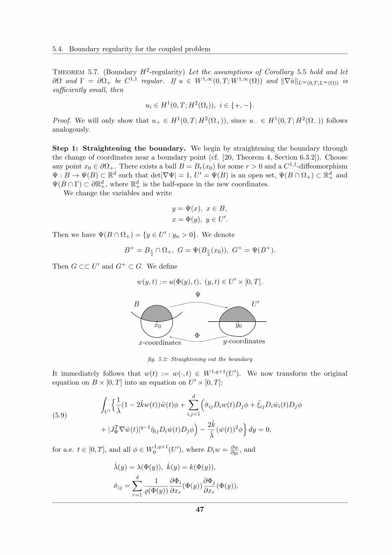
5.4. Boundary regularity for the coupled problem

Theorem 5.7. (Boundary H2-regularity) Let the assumptions of Corollary 5.5 hold and let∂Ω and Γ = ∂Ω+ be C1,1 regular. If u ∈ W 1,∞(0, T ;W 1,∞(Ω)) and ‖∇u‖L∞(0,T ;L∞(Ω)) issufficiently small, then

ui ∈ H1(0, T ;H2(Ωi)), i ∈ +,−.

Proof. We will only show that u+ ∈ H1(0, T ;H2(Ω+)), since u− ∈ H1(0, T ;H2(Ω−)) followsanalogously.

Step 1: Straightening the boundary. We begin by straightening the boundary throughthe change of coordinates near a boundary point (cf. [20, Theorem 4, Section 6.3.2]). Chooseany point x0 ∈ ∂Ω+. There exists a ball B = Br(x0) for some r > 0 and a C1,1-diffeomorphismΨ : B → Ψ(B) ⊂ Rd such that det|∇Ψ| = 1, U ′ = Ψ(B) is an open set, Ψ(B ∩ Ω+) ⊂ Rd+ andΨ(B ∩ Γ) ⊂ ∂Rd+, where Rd+ is the half-space in the new coordinates.

We change the variables and write

y = Ψ(x), x ∈ B,x = Φ(y), y ∈ U ′.

Then we have Ψ(B ∩ Ω+) = y ∈ U ′ : yn > 0. We denote

B+ = B r2∩ Ω+, G = Ψ(B r

2(x0)), G+ = Ψ(B+).

Then G ⊂⊂ U ′ and G+ ⊂ G. We define

w(y, t) := u(Φ(y), t), (y, t) ∈ U ′ × [0, T ].

x0

B

y0

U ′

x-coordinates y-coordinates

Ψ

Φ

fig. 5.2: Straightening out the boundary

It immediately follows that w(t) := w(·, t) ∈ W 1,q+1(U ′). We now transform the originalequation on B × [0, T ] into an equation on U ′ × [0, T ]:

(5.9)

∫U ′

1

λ(1− 2kw(t))w(t)φ+

d∑i,j=1

(σijDiw(t)Djφ+ ξijDiwi(t)Djφ

+ |JTΦ∇w(t)|q−1ηijDiw(t)Djφ)− 2k

λ(w(t))2φ

dy = 0,

for a.e. t ∈ [0, T ], and all φ ∈W 1,q+10 (U ′), where Diw = ∂w

∂yi, and

λ(y) = λ(Φ(y)), k(y) = k(Φ(y)),

σij =d∑r=1

1

%(Φ(y))

∂Φi

∂xr(Φ(y))

∂Φj

∂xr(Φ(y)),

47


ξij(y) =d∑r=1

b(Φ(y))(1− δ(Φ(y)))∂Φi

∂xr(Φ(y))

∂Φj

∂xr(Φ(y)),(5.10)

ηij(y) =

d∑r=1

b(Φ(y))δ(Φ(y))∂Φi

∂xr(Φ(y))

∂Φj

∂xr(Φ(y)).

Note that Drσij , Dr ξij , Drηij ∈ L∞(U ′) for r ∈ 1, . . . , d−1 since Ψ and Φ are C1,1 mappingswhich means they are W 2,∞-regular (see Theorem 3.2). It can be shown (for details see [20,Section 6.3.2]) that

(5.11)

d∑i,j=1

σijφiφj ≥ K1|φ|2,d∑

i,j=1

ξijφiφj ≥ K1|φ|2,

d∑i,j=1

ηijφiφj ≥ K1|φ|2, ∀(y, φ) ∈ U ′ × Rd.

Next, we choose a domain W ′ such that G ⊂⊂ W ′ ⊂⊂ U ′ and select a cut-off function suchthat

ζ = 1 on G, ζ = 0 on Rd \W ′,0 ≤ ζ ≤ 1.

Let |l| > 0 be small and choose r ∈ 1, . . . , d − 1. Note that since we consider directionsparallel to the interface now, we have Dl

rλ = 0, Dlrk = 0 and that there exists a constant

K2 > 0 such that

|Dlrσij(y)| < K2, |Dl

r ξij(y)| < K2, |Dlrηij(y)| < K2(5.12)

for a.e. y ∈W ′, 1 ≤ i, j ≤ d and sufficiently small |l|.

Step 2: Existence of second order derivatives DjDiw ∈ H1(0, T ;L2(G+)), j 6= d.We then use φ = −D−lr (ζ2Dl

rw(t)) as a test function in (5.9), which, after integration withrespect to time, results in

1

2

[∫W ′

1

λl(1− 2klwl)(ζDl

rw)2 dy]t

0+

1

2

[∫W ′

d∑i,j=1

σlijζ2Dl

rDiwDlrDjw dy

]t0

+

∫ t

0

∫W ′

d∑i,j=1

ξlijζ2Dl

rDiwDlrDjw dy ds

=

∫ t

0

∫W ′

2kl

λlDlrwwζ

2Dlrw dy ds+

∫ t

0

∫W ′

kl

λl(wl + 2w)(ζDl

rw)2 dy ds

−∫ t

0

∫W ′

d∑i,j=1

Dlr(σij)Diw (ζ2Dl

rDjw + 2ζDjζDlrw) dy ds

− 2

∫ t

0

∫W ′

d∑i,j=1

σlijDlrDiw ζDjζD

lrw dy ds

48


−∫ t

0

∫W ′

d∑i,j=1

Dlr(ξij)Diw (ζ2Dl

rDjw + 2ζDjζDlrw) dy ds

− 2

∫ t

0

∫W ′

d∑i,j=1

ξijDiw ζDjζDlrw dy ds

−∫ t

0

∫W ′

d∑i,j=1

Dlr(|JTΦ∇w|q−1ηijDiw)(ζ2Dl

rDjw + 2ζDjζDlrw) dy ds.

We can estimate the last term on the right hand side as follows

−∫ t

0

∫W ′

d∑i,j=1

Dlr(|JTΦ∇w|q−1ηijDiw)(ζ2Dl

rDjw + 2ζ(Djζ)Dlrw) dy ds

= −∫ t

0

∫W ′

d∑i,j=1

|(JTΦ∇w)l|q−1ηlijDlrDiw(ζ2Dl


−∫ t

0

∫W ′

d∑i,j=1

Dlr(|JTΦ∇w|q−1ηij)Diw(ζ2Dl


≤C‖∇w‖q−1L∞(0,T ;L∞(W ′))(

d∑i=1

‖ζDlrDiw‖2L2(0,T ;L2(W ′)) + ‖∇ζ‖L∞(0,T ;L∞(W ′))‖∇w‖2L2(0,T ;L2(W ′)))

with C independent of ∇ζ. Due to (5.12) the rest of the terms on the right hand side can beestimated analogously to the estimates in the proof of Theorem 5.2, which for sufficiently small‖∇w‖L∞(0,T ;L∞(W ′)) leads to

‖ζDlrw‖2L∞(0,T ;L2(W ′)) +

d∑i=1

‖ζDlrDiw‖2L∞(0,T ;L2(W ′)) +

d∑i=1

‖ζDlrDiw‖2L2(0,T ;L2(W ′))

≤C((1 + ‖w‖L∞(0,T ;L∞(W ′)))‖∇w‖2L∞(0,T ;L2(W ′))

+ (1 + ‖∇w‖q−1L∞(0,T ;L∞(W ′)))‖∇w‖

2L2(0,T ;L2(W ′)) + |∇w(0)|2L2(W ′) + |w(0)|2H2(W ′)).

Recalling the definition of ζ and employing Lemma 5.1 yields DjDiw ∈ H1(0, T ;L2(G+)) for1 ≤ i ≤ d, 1 ≤ j ≤ d− 1.

Step 3: Existence of second order derivative DdDdw ∈H1(0, T ;L2(G+)). It remainsto show that Dddw := DdDdw ∈ H1(0, T ;L2(G+)). From (5.9), after integration by parts, weobtain

(5.13)

∫G+

σddDdw(t) + ξddDdw(t) + |JTΦ∇w(t)|q−1ηddDdw(t)Ddφdy

=

∫G+

− 1

λ(1− 2kw(t))w(t) +

2k

λ(w(t))2

+

d−1∑j=1

d∑i=1

(Dj(σijDiw(t)) +Dj(ξijDiw(t)) +Dj(|JTΦ∇w(t)|q−1ηijDiw(t))

)φdy,

=:

∫G+

f(w)(t)φdy,

49


for φ ∈ C∞0 (G+), a.e. in [0, T ]. Since the right hand side of the equation is well-defined, weconclude that for a.e. t ∈ [0, T ] the weak derivative of

σddDdw(t) + ξddDdw(t) + |JTΦ∇w|q−1ηddDdw(t)

with respect to yd exists on G+. Furthermore, for a.e. t ∈ [0, T ] the weak derivative satisfies

(5.14) −Dd(σddDdw(t) + ξddDdw(t) + |JTΦ∇w|q−1ηddDdw(t)) = f(w)(t)

on G+. From what we have shown, it follows that f(w) ∈ L2(0, T ;L2(G+)). We set

z(t) := σddDdw(t) + ξddDdw(t) + |JTΦ∇w|q−1ηddDdw(t),

andξdd(t,Ddw(t)) := ξdd + |JTΦ∇w(t)|q−1ηdd,

(suppressing in the notation dependence on D1w(t), . . . , Dd−1w(t) which we already know tobe smooth anyway) so that relation (5.14) reads

−Ddz(t) = f(w)(t),

where

(5.15) z(t) = σddDdw(t) + ξdd(t,Ddw(t))Ddw(t).

Since f(w) ∈ L2(0, T ;L2(G+)), and using the fact that DjDiw ∈ H1(0, T ;L2(G+)) for 1 ≤ i ≤d, 1 ≤ j ≤ d − 1, we have z ∈ L2(0, T ;H1(G+)). On the other hand, due to assuming thatu ∈ W 1,∞(0, T ;W 1,∞(Ω)), we know also that z ∈ L∞(0, T ;L∞(G+)). Therefore, we concludethat

z ∈ L2(0, T ;H1(G+)) ∩ L∞(0, T ;L∞(G+)).

Since (5.15) represents an ODE (pointwise a.e. in space) for Ddw(t), it can be resolved asfollows:

(5.16)

Ddw(t)

= exp(−∫ t

0

σdd

ξdd(τ,Ddw(τ))dτ)(∫ t

0

z(τ)

ξdd(τ,Ddw(τ))exp(∫ τ

0

σdd

ξdd(ρ,Ddw(ρ))dρ)dτ

+Ddw(0)),

and then also Ddw(t) can be expressed in terms of z, σdd, ξdd:

(5.17)

Ddw(t) =z(t)

ξdd(t,Ddw(t))− σdd

ξdd(t,Ddw(t))exp

(−∫ t

0

σdd

ξdd(τ,Ddw(τ))dτ

)(∫ t

0

z(τ)

ξdd(τ,Ddw(τ))exp

(∫ τ

0

σdd

ξdd(ρ,Ddw(ρ))dρ

)dτ +Ddw(0)

).

Since the right hand side depends on Ddw(t), this is a fixed point equation rather than anexplicit expression for Ddw(t). We therefore consider the fixed point operator T : M → M ,defined by the right hand side of (5.17), i.e.,

T = S R,

50


where R : M → M , M = φ ∈ M : φ ≥ K1, is the superposition operator associated withξdd, i.e., R(v)(t) = ξdd(t, v(t)), and S : M →M

S(r)(t) =z(t)

r(t))− σddr(t)

exp

(−∫ t

0

σddr(τ)

dτ

)(∫ t

0

z(τ)

r(τ)exp

(∫ τ

0

σddr(ρ)

dρ

)dτ +Ddw(0)

).

Note that both σdd and ξdd are bounded from below by K1 due to (5.11). We can then concludethat T is a self-mapping on

M = M0 = L∞(0, T ;L∞(G+)),

and onM = M1 = L2(0, T ;H1(G+)) ∩ L∞(0, T ;L∞(G+)) ,

since z ∈ L2(0, T ;H1(G+)) ∩ L∞(0, T ;L∞(G+)). Moreover,

R′(Ddw) =∂

∂v

(ξdd + |JTΦ (D1w, . . . , Dd−1w, v)|q−1ηdd

)|v=Ddw

is small if ‖∇ui‖L∞(0,T ;L∞(Ωi)) and therefore ‖∇w‖L∞(0,T ;L∞(G+)) is small. This implies thatT is a contraction on

M0 = v ∈M0 : ‖v −Ddw‖L∞(0,T ;L∞(G+)) ≤ γ

and onM1 = v ∈M1 : ‖v −Ddw‖L∞(0,T ;L∞(G+)) ≤ γ .

for γ sufficiently small. Thus, the fixed point equation v = T (v) has a unique solution v0

in M0 and it also has a unique solution v1 in M1, and both have to coincide v1 = v0 byuniqueness on M0 ⊇ M1. On the other hand, obviously Ddw lies in M0, solves this fixed pointequation and thus has to coincide with v0, hence also with v1. This proves that Ddw ∈ M1 ⊆L2(0, T ;H1(G+)).

By transforming w back to u, we can conclude that u ∈ H1(0, T ;H2(B+)). The assertionthen follows from the fact that the boundary is compact and can be covered by a finite set ofballs Bri/2(xi)Ni=1.

Higher boundary regularity was obtained under the assumption that u belongs to the spaceW 1,∞(0, T ;W 1,∞(Ω)); this was necessitated by the presence of the q-Laplace damping term inthe equation. The assumption is equivalent to assuming Lipschitz continuity of u in time andspace, i.e. u ∈ C0,1(0, T ;C0,1(Ω)) (see Theorem 3.2). Recall that, thanks to Theorem 4.14 and

the Sobolev embedding W 1,q+1(Ω) → C0,1− d

q+1 (Ω), we know that u is Holder continuous in

space, i.e. u ∈ C0,1(0, T ;C0,1− d

q+1 (Ω)).

5.4.1 Neumann problem for the coupled system. It remains to show H2-regularity upto the boundary for the Neumann problem (5.8).

Theorem 5.8. Let the assumptions of Corollary 5.6 hold, let ∂Ω and Γ = ∂Ω+ be C1,1 regularand let u be the weak solution of (5.8). Furthermore, assume that g ∈ L2(0, T ;H1/2(∂Ω)). Ifu ∈W 1,∞(0, T ;W 1,∞(Ω)) and ‖∇u‖L∞(0,T ;L∞(Ω)) is sufficiently small, then

ui ∈ H1(0, T ;H2(Ωi)), i ∈ +,−.

51


Proof. We will show that u− ∈ H1(0, T ;H2(Ω−)), since the regularity on Ω+ follows as inthe proof of Theorem 5.7. We begin again as before, by straightening the boundary aroundx0 ∈ ∂Ω− \ ∂Ω+. There exists a ball B = Br(x0) for some r > 0 and a C1,1-diffeomorphismΨ : B → Ψ(B) ⊂ Rd such that det|∇Ψ| = 1, U ′ = Ψ(B ∩ Ω−) ⊂ Rd+ is an open set, andΨ(B ∩ ∂Ω−) ⊂ ∂Rd+. We change the variables and write

y = Ψ(x), x ∈ B,x = Φ(y), y ∈ U ′.

We denote G := Ψ(B r2∩ Ω−) ⊂⊂ U ′. We define

w(y, t) := u(Φ(y), t), (y, t) ∈ U ′ × [0, T ],

and transform the orginial equation from (B ∩ Ω)× [0, T ] to U ′ × [0, T ]:

(5.18)

∫U ′

1

λ(1− 2kw(t))w(t)φ+

d∑i,j=1

(σijDiw(t)Djφ+ ξijDiwi(t)Djφ

+ |JTΦ∇w(t)|q−1ηijDiw(t)Djφ)− 2k

λ(w(t))2φ

dy =

∫∂U ′

gφ|J−TΦ n|Rd dx,

for a.e. t ∈ [0, T ], and all φ ∈ W 1,q+1(U ′), and λ, k, σij , ξij , and ηij are defined as in (5.10).We then again use φ = −D−lr (ζ2Dl

rw(t)), r ∈ 1, . . . , d−1 as a test function and proceed withthe estimates like in the proof of Theorem 5.7. The only difference here is the need to estimatethe boundary integral over ∂U ′ appearing in the weak form, therefore we focus our attentionsolely on estimating this term:

−∫ t

0

∫∂U ′

gD−lr (ζ2Dlrw)|J−TΦ n| dx ds

=

∫ t

0

∫B∩∂Ω−

gD−lr (ζ2Dlru) dx ds

≤C‖g‖L2(0,T ;H1/2(∂Ω−))‖ζ2Dl

ru‖L2(0,T ;H1/2(∂Ω−))

≤C‖g‖L2(0,T ;H1/2(∂Ω−))‖ζ2Dl

ru‖L2(0,T ;H1(Ω−))

≤ ε‖ζ2Dlru‖2L2(0,T ;H1(Ω)) +

1

4εC2‖g‖2

L2(0,T ;H1/2(∂Ω−)),

for some conveniently chosen ε > 0. Showing that Dddw ∈ H1(0, T ;L2(G)) follows as in theproof of Theorem 5.7, since we use φ ∈ C∞0 (G) in (5.18).

52

CHAPTER 6

Sensitivity analysis for shape optimization of a focusingacoustic lens in lithotripsy

The present chapter is concerned with a shape optimization problem arising in lithotripsy,where an optimal focusing of the ultrasound waves is needed in order to concentrate theultrasound pressure on the kidney stone and avoid lesions of the surrounding tissue (see fig.1.1). In particular, we are interested in obtaining the first order sensitivity within this context,which will serve as a basis for future development of an efficient optimization algorithm. Forsome first steps taken in the direction of mathematically based optimization of the focusinglens, we refer to the thesis [61] (see also [38]).

The approach to computing the shape derivative that we will take follows the generalframework developed by Ito, Kunisch, and Peichl in [30]. For its extension to a time dependentsetting, we refer to [37]. The main advantage of this variational approach is that it allowsto compute the shape derivative of a cost functional without the need to employ the shapederivative of the state. However, as we will see, assumptions of certain spatial regularity ofthe primal and the adjoint state will be required to obtain the derivative, in particular forobtaining its strong form in terms of boundary integrals.

6.1 Problem formulation

Let Ω ⊂ Rd, d ∈ 1, 2, 3, be a fixed bounded domain with Lipschitz boundary ∂Ω, and, asin the previous chapter, Ω+ a subdomain, representing the lens, such that Ω+ ⊂ Ω and Ω+ hasLipschitz boundary ∂Ω+ = Γ. We denote by Ω− = Ω \Ω+ the part of the domain representingthe fluid region (see fig. 5.2). We then have ∂Ω− = Γ ∪ ∂Ω. Note that the assumptions onthe regularity of the subdomains will eventually have to be strengthened to C1,1 in order toexpress the shape derivative in terms of the boundary integrals over the interface Γ.

We consider the following optimization problem

minΩ+∈Oad

u∈L2(Ω×[0,T ])

J(u,Ω+) ≡ minΩ+∈Oad

u∈L2(Ω×[0,T ])

∫ T

0

∫Ω

(u− ud)2 dx ds,(6.1)

subject to the constraint∫ T

0

∫Ω

1λ(x)(1− 2k(x)u)uφ+ 1

%(x)∇u · ∇φ+ b(x)(1− δ(x))∇u · ∇φ

+b(x)δ(x)|∇u|q−1∇u · ∇φ− 2k(x)λ(x) (u)2φ dx ds = 0

holds for all test functions φ ∈ L2(0, T ;W 1,q+10 (Ω)),

(4.61)

53

Chapter 6. Sensitivity analysis for shape optimization of a focusing lens

with (u, u)|t=0 = (u0, u1), where

(u0, u1) ∈

(u0, u1) ∈W 1,q+10 (Ω)×W 1,q+1

0 (Ω) :

|u1|2L2(Ω) + |∇u0|2L2(Ω) + |∇u1|2L2(Ω) + |∇u1|q+1Lq+1(Ω)

+ |∇u0|2Lq+1(Ω) ≤ κ2T

,

final time T and the size of the initial data κT are determined according to Proposition (4.14).Dependence on Ω+ is not directly visible in (6.1), however this dependence is present via thePDE (i.e. via the equality coinstraint) as will be explained below.

The initial-boundary value problem (4.61) was already stated in Chapter 4, however wehave recalled it here for easier readability.

To formulate the problem it is sufficient to assume that coefficients λ, k, %, b and δ satisfy(5.5), we restate the assumptions here for convenience of the reader:

λ, k, %, b, δ ∈ L∞(Ω),

wi := w|Ωi ∈ C1(Ωi) for w ∈ b, %, λ, δ, k, i ∈ +,−,w := |w|L∞(Ω) for w ∈ b, %, λ, δ, k, δ < 1,

∃%, b, δ : λ ≥ λ > 0, % ≥ % > 0, b ≥ b > 0, δ ≥ δ > 0.

(5.5)

We will, however, eventually return to piecewise constant coefficients (5.7) when calculatingthe shape derivative. As a matter of fact, dependence on Ω+ within the minimization problem(6.1) , (4.61) is just via this interface Γ = ∂Ω+ where discontinuity of the coefficients is allowedto take place.

In (6.1), ud ∈ L2(0, T ;L2(Ω)) denotes the desired acoustic pressure and Oad represents theset of admissible domains and is defined as follows:

Oad = Ω+ : Ω+ ⊂ Ω, Ω+ is open and Lipschitz with uniform Lipschitz constant LO.

We assume that q ≥ 1, q > d − 1 for the state and the adjoint problem to be well-posed;however we will need to strengthen this assumption later to q > 2 in order to prove certainproperties needed for the characterization of the shape derivative.

Note that, due to assumptions (5.5) on the coefficients, (4.61) can be rewritten as∫ T

0

∫Ωλ(x)(1− 2k(x)u)uφ+ %(x)∇u · ∇φ+ b(x)(1− δ(x))∇u · ∇φ

+b(x)δ(x)|∇u|q−1∇u · ∇φ− 2k(x)λ(x)(u)2φ dx ds = 0

holds for all test functions φ ∈ L2(0, T ;W 1,q+10 (Ω)),

(6.2)

with (u, u)|t=0 = (u0, u1), where w(x) = χΩ+1w+

+ (1 − χΩ+) 1w−

for w ∈ λ, % and w(x) =

χΩ+w+ + (1− χΩ+)w− for w ∈ k, b, δ.Let us also restate the strong form of the PDE constraint:

1λ(x)(1− 2k(x)u)u− div( 1

%(x)∇u)− div(b(x)((1− δ(x)) + δ(x)|∇u|q−1)∇u)

= 2k(x)λ(x) (u)2 in Ω+ ∪ Ω−,


1%(x)

∂u∂n+

+ b(x)(1− δ(x)) ∂u∂n+

+ b(x)δ(x)|∇u|q−1 ∂u∂n+

z= 0 on Γ = ∂Ω+,

u = 0 on ∂Ω,

(u, u)|t=0 = (u0, u1).

(5.6)

54

6.1. Problem formulation

Note that the equivalence of formulations (4.61) and (6.2) for sufficiently regular solutions isdue to the fact that (see, for example, [5, 9]):

H1(Ω) = v ∈ L2(Ω) : v|Ωi = vi ∈ H1(Ωi), i ∈ +,−, trΓv+ = trΓv−.

For simplicity of exposition we consider homogeneous Dirichlet boundary conditions on theouter boundary ∂Ω. We mention in passing that Neumann and absorbing boundary conditionsas in [37, 51] and Chapter 4 could be easily incorporated here as well, with some additionalterms involving the Neumann boundary excitation in the analysis of the state equation, butwith no changes in the shape derivative itself, since the outer boundary will not be subject tomodifications.

Some difficulties related to the model (5.6). In [37], the problem of optimizing theexcitation part of the boundary in lithotripsy is considered, with the initial-boundary valueproblem for the Westervelt equation (2.1) as the optimization constraint. This situation ariseswhen excitation and self-focusing of high intensity ultrasound is performed by a piezo-mosaic(see fig. 1.2). Compared to the problem investigated there, the case of focusing by an acousticlens presents us with several additional challenges. Not only a part of the domain boundary isoptimized, but a subdomain which lies in the interior of the domain; this implies providing shapesensitivity analysis for an acoustic-acoustic interface problem. Insufficient spatial regularity ofthe primal (at most W 1,q+1 in space) and the adjoint state (H1 in space) on the whole domaindoes not allow for the shape derivative to be expressed in terms of the boundary integrals.However, as we saw in the previous chapter the state variable exhibits H2-regularity on eachof the subdomains, provided that its gradient remains essentially bounded in space and timeon the whole domain, which we will be able to use in our advantage.

Working with the state equation also implies handling the nonlinear damping term of theq-Laplace type, which is, in terms of shape sensitivity analysis, a nontrivial task as well.

Comment on the notation. To avoid confusion, it should be emphasized that while we usethe dot notation for time differentiation and t ∈ [0, T ] for the physical time variable, in thischapter τ ∈ R will be used for the artificial time variable to indicate varying (sub)domains.If Ω+ is the initial shape of the lens, then Ω+,τ will denote the perturbed lens obtained bymoving points into the direction of some vector field h by some step length τ .

6.1.1 Analysis of the state equation. We recall that the local well-posedness result givenin Proposition 4.14 holds. Since u− ud ∈ L2(0, T ;L2(Ω)), the cost functional is well-defined.

6.1.2 Analysis of the adjoint problem. Since the state equation contains a q-Laplacetype damping term, its linearization provides a significant challenge. The main difficulty inconsidering the linearized q-Laplacian lies in the need for an essential bound on the gradientof the solution u; this is necessary for the linearized operator to be bounded.

We will consider the adjoint problem with the assumption that the weak solution u of (4.61)exhibits the following regularity:

(H1) u ∈ H2(0, T ;W 1,∞(Ω)) ∩X.

Note that the hypothesis is equivalent to assuming Lipschitz continuity of the acoustic pressurein space, i.e. u ∈ H2(0, T ;C0,1(Ω))∩X (cf. Theorem 3.2). Due to the embedding H2(0, T ) →

55


W 1,∞(0, T ), if the hypothesis holds, we also know that u ∈W 1,∞(0, T ;W 1,∞(Ω)).The adjoint problem in weak form is then given by

∫ T0

∫Ω

1λ(1− 2ku)pζ + 1

%∇p · ∇ζ − b(1− δ)∇p · ∇ζ

−bδ(Gu(∇p))· · ∇ζ dx ds =∫ T

0

∫Ω j′(u)ζ dx ds

holds for all test functions ζ ∈ X ′,

(6.3)

with (p, p)|t=T = (0, 0), where j(u) = (u − ud)2, X ′ = L2(0, T ;H1(Ω)) and we have used thenotation

Gu(Y ) := |∇u|q−1Y + (q − 1)|∇u|q−3(∇u · Y )∇u

for the linearized q-Laplace operator. The strong formulation of the adjoint problem then readsas:

1λ(1− 2ku)p− div(1

%∇p) + div(b(1− δ)∇p) + div(bδ(Gu(∇p))·)

= j′(u) in Ω+ ∪ Ω−,

JpK = 0 on Γ,r

1%∂p∂n+− b(1− δ) ∂p

∂n+− bδ (Gu(∇p) · n+)·

z= 0 on Γ,

p = 0 on ∂Ω,

(p, p)|t=T = (0, 0).

(6.4)

To obtain a forward problem, let t ∈ [0, T ] and p(t) := p(T − t), u(t) := u(T − t) (cf. Lemma3.17, [59]); then (p, ˙p)|t=0 = (0, 0), and we have the following problem for p:

∫ T0

∫Ω

1λ(1− 2ku)¨pζ + 1

%∇p · ∇ζ + b(1− δ)∇ ˙p · ∇ζ

+bδ(|∇ ˙u|q−1∇ ˙p− (|∇ ˙u|q−1)·∇p) · ∇ζ

−(q − 1)bδ(

(|∇ ˙u|q−3)·(∇p · ∇ ˙u)∇ ˙u− |∇ ˙u|q−3(∇ ˙p · ∇ ˙u)∇ ˙u

+|∇ ˙u|q−3(∇p · ∇¨u)∇ ˙u+ |∇ ˙u|q−3(∇p · ∇ ˙u)∇¨u)· ∇ζ

dx ds

=∫ T

0

∫Ω j′(u)ζ dx ds,

holds for all test functions ζ ∈ X ′.

(6.5)

Proposition 6.1. (Local well-posedness of the adjoint problem) Let q ≥ 1, q > d − 1,assumptions (5.5) on coefficients and hypothesis (H1) hold. For sufficiently small m, finaltime T > 0, and ‖∇u‖q−2

L∞(0,T ;L∞(Ω))‖∇u‖L∞(0,T ;L∞(Ω)), there exists a unique weak solution

p ∈ X = C1(0, T ;L2(Ω)) ∩H1(0, T ;H10 (Ω)) of (6.4).

Proof. The well-posedness of the adjoint problem can be obtained through standard Galerkingapproximation in space, energy estimates and weak limits (cf. Section 7.2, [20]). We will focus

56

6.1. Problem formulation

here on obtaining the crucial energy estimate. Testing (6.5) with ζ(σ) = ˙p(σ)χ[0,t) (first in adiscretized setting and then via weak limit transferred to the continuous one) yields

1

2

[∫Ω

(1− 2ku(σ))( ˙p(σ))2 dx+

∫Ω

1

%|∇p(σ)|2 dx

]t0

+

∫ t

0

∫Ωb(1− δ)|∇ ˙p|2 dx ds

≤−∫ t

0

∫Ω

k

λ˙u( ˙p)2 dx ds+

∫ t

0

∫Ωj′(u) ˙p dx ds+

∫ t

0

∫Ωbδϕ|∇p||∇ ˙p| dx ds,(6.6)

where

ϕ := |(|∇ ˙u|q−1)·|+ (q − 1)|(|∇ ˙u|q−3)·||∇ ˙u|2 + 2(q − 1)|∇ ˙u|q−2|∇ü| ≤ Cq|∇ ˙u|q−2|∇ü|,

and we have used that∫ t

0

∫Ω bδ |∇ ˙u|q−1|∇ ˙p|2 dx ds ≥ 0 and

∫ t0

∫Ω(q−1)bδ|∇ ˙u|q−3(∇ ˙p ·∇ ˙u)(∇ ˙u ·

∇ ˙p) ≥ 0. By taking essential supremum with respect to t ∈ [0, T ] in (6.6) and employing∫ T

0

∫Ω|ϕ||∇p||∇ ˙p| dx ds

≤Cq‖∇ ˙u‖q−2L∞(0,T ;L∞(Ω))‖∇ü‖L2(0,T ;L∞(Ω))

( 1

4ε‖∇p‖2L∞(0,T ;L2(Ω)) + ε‖∇ ˙p‖2L2(0,T ;L2(Ω))

),

we get the energy estimate for p(1

4(1− a0)− T k

λ(CΩ

H1,L4)2‖u‖L∞(0,T ;L2(Ω))

)‖ ˙p‖2L∞(0,T ;L2(Ω))

+( 1

4%− 1

4εbδ Cq‖∇ ˙u‖q−2

L∞(0,T ;L∞(Ω))‖∇ü‖L2(0,T ;L∞(Ω))

)‖∇p‖2L∞(0,T ;L2(Ω))

+(1

2b(1− δ)− k

λ(CΩ

H1,L4)2‖ ˙u‖L∞(0,T ;L2(Ω))

− εbδ Cq‖∇ ˙u‖q−2L∞(0,T ;L∞(Ω))‖∇ü‖L2(0,T ;L∞(Ω))

)‖∇ ˙p‖2L2(0,T ;L2(Ω))

≤∫ T

0

∫Ωj′(u) ˙p dx ds ≤ 2‖u− ud‖L2(0,T ;L2(Ω))‖ ˙p‖L2(0,T ;L2(Ω)),

with 1 − a0 > 0 and a0 is defined as in (4.4), bounding away from zero factor1 − 2ku. This estimate holds under additional assumptions on smallness of T , m and‖∇ ˙u‖q−2

L∞(0,T ;L∞(Ω))‖∇ü‖L2(0,T ;L∞(Ω)):

Tk

λ(CΩ

H1,L4)2CPm <1

4(1− a0),

1

εbδCq ‖∇ ˙u‖q−2

L∞(0,T ;L∞(Ω))‖∇ü‖L2(0,T ;L∞(Ω)) <1

%,(6.7)

k

λ(CΩ

H1,L4)2CPm <1

2b(1− δ),

and some sufficiently small ε > 0. Here we have employed Poincare’s inequality for functionsin H1

0 (Ω) (see Theorem 2.17, [44] ):

‖ ˙u‖L∞(0,T ;L2(Ω)) ≤ CP‖∇ ˙u‖L∞(0,T ;L2(Ω)) ≤ CPm, u ∈ W,

57


with CP = CP(Ω) > 0. Moreover, we have

| ¨p(t)|H−1(Ω) = supζ∈H1

0 (Ω)\0

(¨p(t), ζ)L2(Ω)

|ζ|H10 (Ω)

= supζ∈H1

0 (Ω)\0

(1−2kuλ

¨p(t), λ1−2ku ζ)L2(Ω)

|ζ|H10 (Ω)

= supζ∈H1

0 (Ω)\0

1

|ζ|H10 (Ω)

∫Ω

−1

%∇p · ∇ζ − b(1− δ)∇ ˙p · ∇ζ

− bδ(|∇ ˙u|q−1∇ ˙p− (|∇ ˙u|q−1)·∇p) · ∇ζ

+ (q − 1)bδ(

(|∇ ˙u|q−3)·(∇p · ∇ ˙u)∇ ˙u− |∇ ˙u|q−3(∇ ˙p · ∇ ˙u)∇ ˙u

+ |∇ ˙u|q−3(∇p · ∇ü)∇ ˙u+ |∇ ˙u|q−3(∇p · ∇ ˙u)∇ü)· ∇ζ + j′(u)ζ

dx ,

where ζ = λ1−2ku ζ, hence

|∇ζ|L2(Ω) =

∣∣∣∣∣ λ

1− 2ku∇ζ +

2kλζ

(1− 2ku)2∇u

∣∣∣∣∣L2(Ω)

≤ λ

1− a0|∇ζ|L2(Ω) +

2kλ

(1− a0)2|ζ|L6(Ω)|∇u|L3(Ω).

This further implies

| ¨p(t)|H−1(Ω) ≤C(|∇p(t)|L2(Ω)|∇ ˙u(t)|q−2L∞(Ω)|∇ü(t)|L∞(Ω)

+ |∇ ˙p(t)|L2(Ω)|∇ ˙u(t)|q−1L∞(Ω) + |u(t)− ud(t)|L2(Ω)),

with C = C(k, λ, %, b, δ, q) > 0. By squaring and integrating over (0, T ), we can achieve that¨p ∈ L2(0, T ;H−1(Ω)).

According to Theorem 3, Section 5.9, [20], since ˙p ∈ L2(0, T ;H10 (Ω)) and ¨p ∈

L2(0, T ;H−1(Ω)), it follows that ˙p ∈ C(0, T ;L2(Ω)). The statement then comes from reversingthe time transformation.

6.2 Elements of shape optimization

To be able to define the shape derivative of our cost functional, we need to introduceperturbations of the domain in a suitable way. To this end, we employ the so called perturbationof the identity transformations. We introduce a fixed vector field h ∈ C1,1(Ω,Rd) with h|∂Ω = 0,and a family of transformations Fτ : Ω 7→ Rd

Fτ = id+ τh, for τ ∈ R.

It can be shown that there exists τ0 > 0, such that for |τ | < τ0, Fτ is a C1,1-diffeomorphism(cf. [29]). If the perturbed lens is given by Ω+,τ = Fτ (Ω+) and Γτ = Fτ (Γ), then it followsthat Γτ is Lipschitz continuous (see [28, Theorem 4.1]).

58

6.2. Elements of shape optimization

Ω+

Γ

Ω

Ω−

Ω

Ω+,τ

Γτ

Ω−,τFτ

fig. 6.1: Fixed and perturbed subdomains

We mention that perturbations could be described alternatively by the velocity method as theflow determined by the initial-value problem

ξ(τ) = h(ξ(τ))

ξ(0) = x,

with Fτ (x) = ξ(τ ; 0, x).The Eulerian derivative of J at Ω+ in the direction of the vector field h is defined as

dJ(u,Ω+)h = limτ→0

1

τ(J(uτ ,Ω+,τ )− J(u,Ω+)),

where uτ satisfies the state equation on the domain with the perturbed lens Ω+,τ . Thefunctional J is said to be shape differentiable at Ω+ if dJ(u,Ω+)h exists for all h ∈ C1,1(Ω,Rd)and defines a continuous linear functional on C1,1(Ω,Rd).

We introduce the following notation:

(6.8) Iτ = det(DFτ ) , Aτ = (DFτ )−T .

where DFτ is the Jacobian of the transformation Fτ .

Lemma 6.2. [30] For sufficiently small τ0 > 0, mapping Fτ has the following properties:

τ 7→ Fτ ∈ C1(−τ0, τ0;C1(Ω,Rd)) τ 7→ Aτ ∈ C(−τ0, τ0;C(Ω,Rd×d))τ 7→ Fτ ∈ C(−τ0, τ0;C1,1(Ω,Rd)) τ 7→ Iτ ∈ C1(−τ0, τ0;C(Ω))

τ 7→ F−1τ ∈ C(−τ0, τ0;C1(Ω,Rd)) F0 = id

d

dτFτ |τ=0 = h

d

dτF−1τ |τ=0 = −h

d

dτDFτ |τ=0 = Dh

d

dτDF−1

τ |τ=0 =d

dτ(Aτ )T |τ=0 = −Dh

d

dτIτ |τ=0 = divh.

d

dτAτ |τ=0 = −(Dh)T .

As a consequence of Lemma 6.2, there exist α0, α1 > 0 such that

0 < α0 ≤ Iτ (x) ≤ α1, for x ∈ Ω, τ ∈ [−τ0, τ0].(6.9)

Furthermore, there exist β1, β2 > 0 such that

|Aτ |L∞(Ω) ≤ β1, |A−1τ |L∞(Ω) ≤ β2, for τ ∈ [−τ0, τ0].(6.10)

We will often employ the following lemma which gives us the formula for the transformationof domain integrals:

59


Lemma 6.3. [56] Let ϕτ ∈ L1(Ωτ ), then ϕτ Fτ ∈ L1(Ω) and∫Ωτ

ϕτ dxτ =

∫Ω

(ϕτ Fτ ) Iτ dx.

Finally, let us recall the well-known result obtained by Zolesio in 1979 which describes thestructure of the shape gradient for sufficiently smooth domains:

Theorem 6.4. [[14], Theorem 3.6, Corollary 1, Chapter 9] Let J be a real-valued shapefunctional. Assume that J is shape differentiable at some Ω+ ⊂ Rd with boundary Γ.

(i) The support of the shape gradient is contained in Γ.

(ii) Let m ≥ 0 be the smallest integer such that the map h 7→ J(Ω+)h : Cmc (Rd,Rd) → R iscontinuous. If the boundary Γ is of order Cm+1, then there exists a scalar distributiong(Γ) in Rd with support in Γ such that g(Γ) ∈ (Cm(Γ))? and for all h ∈ Cmc (Rd,Rd)

dJ(Ω+)h = 〈g(Γ), trΓ h · n〉Cm(Γ).

(iii) If g ∈ L1(Γ), then

dJ(Ω+)h =

∫Γgh · ndΓ.

The last formula is commonly called the Hadamard formula.

6.3 Existence of optimal shapes

From now on, for simplicity of exposition, we assume that all the coefficients in the stateequation are piecewise constants, i.e.

λ, k, %, b, δ ∈ L∞(Ω),

wi := w|Ωi is constant, for w ∈ b, %, λ, δ, k, i ∈ +,−,wi > 0 for w ∈ b, %, λ, δi ∈ (0, 1), ki ∈ R.

(5.7)

Note that now ω = min|ω+|, |ω−|, ω = max|ω+|, |ω−|, where ω ∈ b, %, λ, δ, k.We turn next to the question of existence of minimizers for the shape optimization problem

(6.1) subject to the constraint (4.61), with the coefficients satisfying assumptions (5.7). Themain idea of the proof is to employ the Bolzano-Weierstrass theorem for continuous functionson compact sets (for this approach see, for instance, [24, Section 3] and [41, Section 3.2]).

We recall that given two nonempty sets A and B in Rd, their Hausdorff distance is definedas

dH(A,B) = maxsupx∈A

infy∈B|y − x|, sup

y∈Binfx∈A|y − x|.

The following compactness result holds:

Theorem 6.5. [[24], Theorem 2] Let Ωn+ be a sequence in Oad. Then there exists Ω?

+ ∈ Oad

and a subsequence Ωnk+ which converges to Ω?

+ in the sense of Hausdorff, and in the sense

of characteristic functions. Additionally, Ω+nk

and ∂Ω+nk

converge in the sense of Hausdorff

towards Ω?+ and ∂Ω?

+, respectively.

60

6.3. Existence of optimal shapes

Here the set of characteristic functions is defined as

Char(Ω) = χΩ+ : Ω+ ⊂ Ω is measurable ∧ χΩ+(1− χΩ+) = 0 a.e. in Ω

and convergence on this set, first of all, means pointwise almost everywhere convergence offunctions, but due to Lebesgue’s dominated convergence theorem also convergence in Lr(Ω)for any r ∈ [1,∞).

We first establish continuity of the mapping Ω+ 7→ u, where u solves the weak form (6.2)of (5.6).

Proposition 6.6. Let q ≥ 1, q > d − 1 and the assumptions (5.7) on the coefficients in(5.6) hold. Then the mapping χΩ+ 7→ u is continuous from the set of characteristic functions

Char(Ω) to W 1,∞(0, T ;L2(Ω)) ∩W 1,q+1(0, T ;W 1,q+10 (Ω)).

If additionally there exists ε > 0 such that the solution u] of (4.61) with Ω+ = Ω]+ satisfies

‖u]‖W 1,q+1(0,T ;W 1,q+1+ε(Ω)) ≤ C,(6.11)

where C depends only on Ω and the final time T , then the mapping χΩ+ 7→ u is even Holdercontinuous at χ

Ω]+.

Proof. Let Ωn+ be a sequence converging to Ω]

+ in the sense of characteristic functions. Bysubtracting the weak forms (6.2) for un and u], corresponding to the domains with the lens

regions Ωn+ and Ω]

+ respectively, we get

∑i∈+,−

∫ T

0

∫Ω 1

λi(1− 2kiu

n)(un − u])φ− 2kiλi

(un − u])u]φ+1

%i∇(un − u]) · ∇φ

+ bi(1− δi)∇(un − u]) · ∇φ+ biδi(|∇un|q−1∇un − |∇u]|q−1∇u]) · ∇φ

− 2kiλi

((un)2 − (u]i)2)φχΩni

dx ds

=∑

i∈+,−

∫ T

0

∫Ω 1

λi(1− 2kiu

])u]φ+1

%i∇u] · ∇φ+ bi(1− δi)∇u] · ∇φ

+ biδi|∇u]|q−1∇u] · ∇φ− 2kiλi

(u])2φ (χΩni− χ

Ω]i) dx ds,

with Ωn− = Ω \ Ω

n+, Ω]

− = Ω \ Ω]+. Testing with φ = un − u] and employing inequality (3.12)

for the difference of the q-Laplace terms then yields

1

2λ(1− 2k‖un‖L∞(0,T ;L∞(Ω)))‖un − u]‖2L∞(0,T ;L2(Ω)) +

1

2%‖∇(un − u])‖2L2(0,T ;L2(Ω))

+ b(1− δ)‖∇(un − u])‖2L2(0,T ;L2(Ω)) + 21−qbδ‖∇(un − u])‖q+1Lq+1(0,T ;Lq+1(Ω))

≤ 2k

λ(‖u]‖L2(0,T ;L∞(Ω))‖un − u]‖2L∞(0,T ;L2(Ω))

+ (CΩH1

0 ,L4)2‖un − u]‖L∞(0,T ;H1

0 (Ω))‖u]‖L2(0,T ;L2(Ω))‖un − u]‖L2(0,T ;H10 (Ω))

+∑

i∈+,−

∣∣∣∫ T

0

∫Ω

1

λi(1− 2kiu

])u](un − u]) +1

%i∇u] · ∇(un − u])

61


+ bi(1− δi)∇u] · ∇(un − u]) + biδi|∇u]|q−1∇u] · ∇(un − u])

− 2kiλi

(u])2(un − u])

(χΩni− χ

Ω]i) dx ds

∣∣∣.By employing the Sobolev embedding W 1,q+1

0 (Ω) → L∞(Ω):

‖u]‖L2(0,T ;L∞(Ω)) ≤ CΩW 1,q+1

0 ,L∞‖u]‖

L2(0,T ;W 1,q+10 (Ω))

and then utilizing the energy estimate (4.63) from Proposition 4.14 to estimate the terms‖u]‖

L2(0,T ;W 1,q+10 (Ω))

and ‖u]‖L2(0,T ;L2(Ω)), we conclude that for sufficiently small initial data

the two first terms on the right hand side can be absorbed by the appropriate terms on the lefthand side. For the remaining terms, we employ the following estimates:∫ T

0

∫Ω

1

λ(1− 2kiu

])u](un − u])(χΩni− χ

Ω]i) dx ds

≤ (1 + 2k‖u]‖L∞(0,T ;L∞(Ω)))‖u]‖L2(0,T ;L2(Ω))‖un − u]‖L2(0,T ;Lq+1(Ω))|χΩni− χ

Ω]i|Lr1 (Ω),

together with ∫ T

0

∫Ω

2kiλi

(u])2(un − u])(χΩni− χ

Ω]i) dx ds

≤ 2k

λ‖u]‖2L∞(0,T ;L∞(Ω))‖u

n − u]‖L2(0,T ;L2(Ω))|χΩni− χ

Ω]i|L2(Ω),

and the estimate∫ T

0

∫Ω

1

%∇u] · ∇(un − u])(χΩni

− χΩ]i

) dx ds

≤ 1

%‖∇u]‖L2(0,T ;L2(Ω))‖∇(un − u])‖L2(0,T ;Lq+1(Ω))|χΩni

− χΩ]i|Lr(Ω)

≤ 1

%T

1r1 ‖∇u]‖L2(0,T ;L2(Ω))‖∇(un − u])‖Lq+1(0,T ;Lq+1(Ω))|χΩni

− χΩ]i|Lr1 (Ω),

with r1 = 2(q+1)q−1 . An estimate analogous to the last one can be derived for the bi(1− δi)-term

where ∇u] is replaced by ∇u]. Thus all these terms on the right hand side tend to zero asn→∞.

Finally, by Lebesgue’s dominated convergence theorem 3.10 also the integral∫ T

0

∫Ωbiδi|∇u]|q−1∇u] · ∇(un − u])(χΩni

− χΩ]i

) dx ds(6.12)

goes to zero as n→∞, since its integrand, due to the factor χΩni−χ

Ω]i, tends to zero pointwise

a.e. and is bounded by the integrable function bδ|∇u]|q(|∇un| + |∇u]|) whose integral isbounded by bδ‖∇u]‖q

Lq+1(0,T ;Lq+1+ε(Ω))(‖∇un‖Lq+1(0,T ;Lq+1(Ω)) + ‖∇u]‖Lq+1(0,T ;Lq+1(Ω))). This

proves the assertion.If we additionally assume that the solution of the state problem exhibits a slightly higher

regularity in space than W 1,q+1(Ω), namely that u ∈W 1,q+1(0, T ;W 1,q+1+ε(Ω)) for some ε > 0,we can estimate (6.12) as∫ T

0

∫Ωbiδi|∇u]|q−1∇u] · ∇(un − u])(χΩni

− χΩ]i

) dx ds

62

6.3. Existence of optimal shapes

≤ bδ‖∇u]‖qLq+1(0,T ;Lq+1+ε(Ω))

‖∇(un − u])‖Lq+1(0,T ;Lq+1(Ω))|χΩni− χ

Ω]i|Lr2 (Ω),

with r2 = (1+q)(1+ε)qε . Altogether, we can then conclude that

(1− 2k‖un‖L∞(0,T ;L∞(Ω)))‖un − u]‖2L∞(0,T ;L2(Ω)) + ‖∇(un − u])‖2L2(0,T ;L2(Ω))

+ ‖∇(un − u])‖2L2(0,T ;L2(Ω)) + ‖∇(un − u])‖q+1Lq+1(0,T ;Lq+1(Ω))

≤C((1 + 2k‖u]‖L∞(0,T ;L∞(Ω)))‖u]‖L2(0,T ;L2(Ω))‖un − u]‖L2(0,T ;Lq+1(Ω))|χΩn+− χ

Ω]+|Lr1 (Ω)

+ ‖∇u]‖L2(0,T ;L2(Ω))‖∇(un − u])‖Lq+1(0,T ;Lq+1(Ω))|χΩn+− χ

Ω]+|Lr1 (Ω)

+ ‖∇u]‖L2(0,T ;L2(Ω))‖∇(un − u])‖Lq+1(0,T ;Lq+1(Ω))|χΩn+− χ

Ω]+|Lr1 (Ω)

+ ‖∇u]‖qLq+1(0,T ;Lq+1+ε(Ω))

‖∇(un − u])‖Lq+1(0,T ;Lq+1(Ω))|χΩn+− χ

Ω]+|Lr2 (Ω)

+ ‖un‖2L∞(0,T ;L∞(Ω))‖un − u]‖L2(0,T ;L2(Ω))|χΩn+

− χΩ]+|L2(Ω)),

for sufficiently large C > 0 independent of n, which implies Holder continuity of the mappingχΩ+ 7→ u.

Now let Ωn+ be a minimizing sequence for (6.1), (4.61). Due to Theorem 6.5, there exists

a subsequence, which, for brevity, we still denote Ωn+, that converges to some Ω?

+ ∈ Oad. Byextracting another sequence, we may as well assume that Ωn

+ → Ω?+ in the sense of characteristic

functions.Let us denote by un the weak solution corresponding to the domain where the lens region

is given by Ωn+. We know then that un satisfies the estimate (4.63), where u is interchanged

with un. This means that we may extract a subsequence, again denoted un, such that

un u? in H2(0, T ;L2(Ω)),

∇un ∇u? in Lq+1(0, T ;Lq+1(Ω)).

Due to the embedding H2(0, T ) → C1(0, T ), this further implies that u(t) u?(t) and u(t) u?(t) in L2(Ω) for all t ∈ [0, T ]. Therefore, (u?, u?)|t=0 = (u0, u1).

It remains to show that u? solves the state problem on the domain whose lens region isgiven by Ω?

+.

Proposition 6.7. Let the assumptions of Proposition 6.6 be satisfied. Let Ωn+ be a minimizing

sequence for the shape optimization problem (6.1), (4.61), and let Ω?+ be an accumulation

point of this sequence in accordance with Theorem 6.5. Then the sequence un correspondingto the domain with the lens region Ωn

+ converges strongly to u? in W 1,∞(0, T ;L2(Ω)) ∩W 1,q+1(0, T ;W 1,q+1

0 (Ω)), where u? is the solution of (4.61) in the domain whose lens region isgiven by Ω?

+.

Proof. In order to see that u? is the weak solution of the state problem in the domain wherethe lens region is given by Ω?

+, note that due to the fact that un solves (4.61) with lens regionΩn

+ and using integration by parts in the first term on the right hand side

∑i∈+,−

∫ T

0

∫Ω 1

λi(1− 2kiu

?)u?φ+1

%i∇u? · ∇φ+ bi(1− δi)∇u? · ∇φ

+ biδi|∇u?|q−1∇u? · ∇φ− 2kiλi

(u?)2φχΩ?idx ds

63


=∑

i∈+,−

∫ T

0

∫Ω− 1

λi(1− 2kiu

?)(u? − un)φ− 2kiλi

(u? − un)unφ+1

%i∇(u? − un) · ∇φ

+ bi(1− δi)∇(u? − un) · ∇φ+ biδi(|∇u?|q−1∇u? − |∇un|q−1∇un) · ∇φ(6.13)

− 2kiλi

(u? − un)(u? + un)φχΩ?idx ds

+∑

i∈+,−

∫ T

0

∫Ω 1

λi(1− 2kiu

n)unφ+1

%i∇un · ∇φ+ bi(1− δi)∇un · ∇φ

+ biδi|∇un|q−1∇un · ∇φ−2kiλi

(un)2φ(χΩ?i− χΩni

) dx ds,

for all φ ∈ C∞(0, T ;C∞0 (Ω)), φ(T ) = 0. The difference of the q-Laplace terms on the righthand side can be estimated with the help of inequality (3.11) (with η = 0) as follows:∫ T

0

∫Ωbiδi(|∇u?|q−1∇u? − |∇un|q−1∇un) · ∇φχΩ?i

dx ds

≤Cqbδ∫ T

0

∫Ω|∇(u? − un)|(|∇u?|q−1 + |∇un|q−1)|∇φ||χΩ?i

| dx ds

≤Cqbδ‖∇(u? − un)‖Lq+1(0,T ;Lq+1(Ω))

(‖∇u?‖q−1

Lq+1(0,T ;Lq+1(Ω))

+ ‖∇un‖q−1Lq+1(0,T ;Lq+1(Ω))

)‖∇φ‖Lq+1(0,T ;Lq+1(Ω)).

The remaining terms can be estimated analogously to the estimates in the proof of Proposition6.6, from which it then follows that the right hand side in (6.13) tends to zero as n→∞.

Theorem 6.8. Let q ≥ 1, q > d−1 and the assumptions (5.7) on the coefficients in (5.6) hold.Then the shape optimization problem (6.1) subject to (4.61) has a solution.

Proof. Let us define the reduced cost functional J : Oad → R:

J(Ω+) = J(u(Ω+),Ω+).

Let Ωn+ → Ω?

+ as n→∞. It can be shown (cf. [41, Lemma 3.3]) that

|J(u?,Ω?+)− J(un,Ωn

+)| ≤ ‖u? − un‖L2(0,T ;L2(Ω))‖u? + un − 2ud‖L2(0,T ;L2(Ω)).

Since the term ‖u? + un − 2ud‖L2(0,T ;L2(Ω)) is uniformly bounded due to (4.63), by employingProposition 6.6 we achieve that the right hand side tends to zero as n → ∞. Therefore thecost functional J is continuous on Oad. According to the Bolzano-Weierstrass theorem 3.12,since Oad is compact, J attains a global minimum on Oad.

6.4 State equation on the domain with perturbed lens

Let us introduce, for some Lipschitz domain Ω+ ∈ Oad, the operator E(·,Ω+) : W → X?

by

(6.14)

〈E(u,Ω+), φ〉X?,X =∑

i∈+,−

∫ T

0

∫Ωi

1

λi(1− 2kiu)uφ+

1

%i∇u · ∇φ

+ bi(1− δi)∇u · ∇φ+ biδi|∇u|q−1∇u · ∇φ− 2kiλi

(u)2φ dx ds.

64

6.4. State equation on the domain with perturbed lens

Fix τ ∈ (−τ0, τ0). Proposition 4.14 guarantees that E(u,Ω+,τ ) = 0 has a unique solution,which we denote uτ : Ω → R. We transport uτ back to the domain with the fixed lens Ω+ bydefining uτ : Ω→ R as

uτ = uτ Fτ .

Differentiability of h implies that uτ ∈ X. We further have

(6.15)

〈E(uτ ,Ω+,τ ), φτ 〉X?τ ,Xτ

=∑

i∈+,−

∫ T

0

∫Ωi,τ

1

λi(1− 2kiuτ )uτφτ +

1

%i∇uτ · ∇φτ

+ bi(1− δi)∇uτ · ∇φτ + biδi|∇uτ |q−1∇uτ · ∇φτ −2kiλi

(uτ )2φτ

dxτ ds

=∑

i∈+,−

∫ T

0

∫Ωi

1

λi(1− 2kiu

τ )uτφτ +1

%iAτ∇uτ ·Aτ∇φτ

+ bi(1− δi)Aτ∇uτ ·Aτ∇φτ + biδi|Aτ∇uτ |q−1Aτ∇uτ ·Aτ∇φτ

− 2kτ

λi(uτ )2φτ

Iτ dx ds

≡ 〈E(uτ , τ), φτ 〉X?,X ,

for any φτ ∈ Xτ = X, with Ω−,τ = Ω \Ω+,τ , where we have used Lemma 6.3 and the fact that

∇uτ = Aτ∇uτ F−1τ .

Therefore, for sufficiently small |τ |, uτ uniquely satisfies an equation on the domain with thefixed lens:

E(uτ , τ) = 0.(6.16)

Since F0 = id, we have that u0 = u and E(u, 0) = E(u,Ω+).

6.4.1 Continuity of the state with respect to domain perturbations. We will nowfocus our attention on the speed of convergence of uτ to u as τ → 0 and prove two propertieswhich together correspond to hypothesis (H2) in [30] (see also [29, Proposition 3.1]).

We begin with the question of uniform boundedness of uτ with respect to τ ∈ (−τ0, τ0).Since

‖uτ‖L∞(0,T ;L∞(Ω)) = ‖uτ Fτ‖L∞(0,T ;L∞(Ω))

≤‖uτ‖L∞(0,T ;L∞(Ω)),

we also have that

1− a0 < ‖1− 2kuτ‖L∞(0,T ;L∞(Ω)) < 1 + a0,(6.17)

where a0 is defined as in (4.4).

Proposition 6.9. Let q ≥ 1, q > d − 1 and assumptions (5.7) hold. Solutions uτ of (6.16)are uniformly bounded in W 1,∞(0, T ;L2(Ω)) ∩W 1,q+1(0, T ;W 1,q+1

0 (Ω)) for τ ∈ (−τ0, τ0).

65


Proof. It can be shown (similarly to [29, Lemma 3.3]) that

‖∇uτ‖Lq+1(0,T ;Lq+1(Ω)) ≤1 + τ0|Dh|L∞(Ω)

α1/(q+1)0

‖∇uτ‖Lq+1(0,T ;Lq+1(Ω)).

with α0 as in (6.9) This implies that, for uτ ∈ W, we can estimate

‖∇uτ‖Lq+1(0,T ;Lq+1(Ω)) ≤1 + τ0|Dh|L∞(Ω)

α1/(q+1)0

M.(6.18)

Testing (6.16) with φτ = uτχ[0,t) ∈ L2(0, T ;W 1,q+10 (Ω)), with E as in (6.15), yields

1

2

[∫Ω

1

λ(1− 2kuτ )(uτ )2Iτ dx

]t0

+1

2

[∫Ω

1

%|Aτ∇uτ |2Iτ dx

]t0

+

∫ t

0

∫Ωb(1− δ)|Aτ∇uτ |2Iτ dx ds+

∫ t

0

∫Ωbδ|Aτ∇uτ |q+1Iτ dx ds

=

∫ t

0

∫Ω

k

λ(uτ )3Iτ dx ds.

By taking the supremum over t ∈ [0, T ] and by utilizing the uniform boundedness properties(6.9), (6.10) and estimates (6.17) and (6.18), we find that

1

4

α0

λ(1− a0)‖uτ‖2L∞(0,T ;L2(Ω)) +

1

4

1

λ

1

β22

α0‖∇uτ‖2L∞(0,T ;L2(Ω))

+1

2b(1− δ) 1

β22

α0‖∇uτ‖2L2(0,T ;L2(Ω)) +1

2bδ

1

βq+12

α0‖∇uτ‖q+1Lq+1(0,T ;Lq+1(Ω))

≤ k

λα1‖uτ‖L2(0,T ;L∞(Ω))

√T‖uτ‖2L∞(0,T ;L2(Ω)) +

1

2λ(1 + a0)α1|u1|2L2(Ω)

+1

2%α1|∇u0|2L2(Ω)(6.19)

≤ k

λα1C

ΩW 1,q+1

0 ,L∞T

qq+1

1 + τ0|Dh|L∞(Ω)

α1/(q+1)0

M‖uτ‖2L∞(0,T ;L2(Ω)) +1

2λ(1 + a0)α1|u1|2L2(Ω)

+1

2%α1|∇u0|2L2(Ω).

From here, for sufficiently small M and T , we can achieve that the first term on the righthand side gets absorbed by the appropriate term on the left hand side. Thus we have uniformboundedness of uτ in W 1,∞(0, T ;L2(Ω)) ∩W 1,q+1(0, T ;W 1,q+1

0 (Ω)), |τ | < τ0.

The Holder continuity of u with respect to domain perturbations is established by our nextresult.

Proposition 6.10. Let q ≥ 1, q > d− 1 and let assumptions (5.7) hold. Then

(6.20)limτ→0

1

τ

(‖uτ − u‖2L∞(0,T ;L2(Ω)) + ‖∇(uτ − u)‖2L∞(0,T ;L2(Ω))

+ ‖∇(uτ − u)‖2L2(0,T ;L2(Ω)) + ‖∇(uτ − u)‖q+1Lq+1(0,T ;Lq+1(Ω))

)= 0.

66


Proof. Note that the difference vτ = u− uτ satisfies

(6.21)

∑i∈+,−

∫ T

0

∫Ωi

1

λi(1− 2kiu

τi )vτi φiIτ −

2kiλivτi uiφiIτ +

1

%i∇vτi · ∇φi

+ bi(1− δi)∇vτi · ∇φi + biδi(|∇ui|q−1∇ui − |∇uτi |q−1∇uτi ) · ∇φi

− 2kiλi

(ui + uτi )vτi φi

dx ds

= 〈f+, φ+〉X?+,X+

+ 〈f−, φ−〉X?−,X−

,

for all φ ∈ X, with the two terms on the right hand side given by

〈fi, φi〉X?i ,Xi

=

∫ T

0

∫Ωi

1

λi(Iτ − 1)(1− 2kiui)uiφi +

1

%i

((Iτ − 1)Aτ∇uτi ·Aτ∇φi

+ (Aτ − I)∇uτi ·Aτ∇φi +∇uτi · (Aτ − I)∇φi)

+ bi(1− δi)(

(Iτ − 1)Aτ∇uτi ·Aτ∇φi + (Aτ − I)∇uτi ·Aτ∇φi +∇uτi · (Aτ − I)∇φi)

+ biδi

((|Aτ∇uτi |q−1Aτ∇uτi − |∇uτi |q−1∇uτi ) · ∇φi + |Aτ∇uτi |q−1Aτ∇uτi · (Aτ − I)∇φi

+ (Iτ − 1)|Aτ∇uτi |q−1Aτ∇uτi ·Aτ∇φi)− (Iτ − 1)

2kiλi

(uτi )2φi

dx ds,

where Xi = L2(0, T ;W 1,q+1(Ωi)). Since φi = vτi χ[0,t) ∈ X, we can use it as test functions in(6.21), which together with the uniform boundedness of Iτ results in∑

i∈+,−

[1

2α0

∫Ωi

1

λi(1− 2kiu

τi )(vτi )2 dx+

1

2

∫Ωi

1

%i|∇vτi |2 dx

]t0

+

∫ t

0

∫Ωi

bi(1− δi)|∇vτi |2 dx ds+

∫ t

0

∫Ωi

biδi21−q |∇vτi |q+1 dx ds

≤

∑i∈+,−

kλ

[α1‖uτi ‖L2(0,T ;L∞(Ωi))‖v

τi ‖2L∞(0,T ;L2(Ωi))

+ 2(CΩiH1,L4)2α1‖ui‖L2(0,T ;L2(Ωi))‖v

τi ‖L∞(0,T ;H1(Ωi))‖vi‖L2(0,T ;H1(Ωi))

+ 2(‖uτi ‖L2(0,T ;L∞(Ωi)) + ‖ui‖L2(0,T ;L∞(Ωi)))‖vτi ‖2L∞(0,T ;L2(Ωi))

]+ |〈fi, vτi 〉X?

i ,Xi|.

Here we have also utilized the fact that

(|∇ui|q−1∇ui − |∇uτi |q−1∇uτi ) · ∇(ui − uτi ) ≥ 21−q |∇(ui − uτi )|q+1,

which follows from inequality (3.12).We can employ

‖uτi ‖L2(0,T ;L∞(Ωi)) ≤ Tq−1

2(q+1)CΩiW 1,q+1,L∞

‖uτi ‖Lq+1(0,T ;W 1,q+1(Ωi)),(6.22)

and the same inequality with ui instead of uτi , as well as

‖vτi ‖L∞(0,T ;H1(Ωi)) ≤√T‖vτi ‖L2(0,T ;H1(Ωi)),

67


(since vτi |t=0 = vτi |t=0 = 0) to conclude that, because ‖uτi ‖Lq+1(0,T ;W 1,q+1(Ωi)) is uniformlybounded for τ ∈ (−τ0, τ0), for sufficiently small m and final time T it holds

(6.23)

∑i∈+,−

(‖vτ‖2L∞(0,T ;L2(Ω)) + ‖∇vτ‖2L∞(0,T ;L2(Ω)) + ‖∇vτ‖2L2(0,T ;L2(Ω))

+ ‖∇vτ‖q+1Lq+1(0,T ;Lq+1(Ω))

)

≤C(|〈f+, vτ+〉X?

+,X+|+ |〈f−, vτ−〉X?

−,X−|),

for some sufficiently large C > 0 which does not depend on τ . By employing the inequality(3.11) (with η = 0) we obtain

(6.24)|(|Aτ∇uτi |q−1Aτ∇uτi − |∇uτi |q−1∇uτi )∇vi|≤Cq |(Aτ − I)∇uτi | (|∇uτi |q−1 + |(Aτ − I)∇uτi |q−1) |∇vi|.

We can therefore estimate the terms on the right hand side in (6.23) as

(6.25)

|〈fi, vτi 〉X?i ,Xi|

≤ 1

λ|Iτ − 1|L∞(Ωi)(1 + a0)‖ui‖L2(0,T ;L2(Ωi))‖v

τi ‖L2(0,T ;L2(Ωi))

+ (|Iτ − 1|L∞(Ωi)β21 + |Aτ − I|L∞(Ωi)(1 + β1))

(1

%‖∇uτi ‖L2(0,T ;L2(Ωi))

+ b(1− δ)‖∇uτi ‖L2(0,T ;L2(Ωi))

)‖∇vτi ‖L2(0,T ;L2(Ωi))

+ bδ(q|Aτ − I|L∞(Ωi)(1 + |Aτ − I|q−1

L∞(Ωi)) + |Aτ − I|L∞(Ωi)β

q1

+ |Iτ − 1|L∞(Ωi)βq+11

)‖∇uτi ‖

qLq+1(0,T ;Lq+1(Ωi))

‖∇vτi ‖Lq+1(0,T ;Lq+1(Ωi))

+ |Iτ − 1|L∞(Ωi)2k

λ(CΩi

H1,L4)2‖uτi ‖2L2(0,T ;H1(Ωi))‖vτi ‖L∞(0,T ;L2(Ωi)),

where a0 is defined as in (4.4). By inserting this into the estimate (6.23) and by employing theuniform boundedness result from Proposition 6.9, properties of the mapping Fτ from Lemma6.2 and Young’s inequality, we can conclude that

(6.26)

limτ→0

∑i∈+,−

(‖vτ‖2L∞(0,T ;L2(Ω)) + ‖∇vτ‖2L∞(0,T ;L2(Ω)) + ‖∇vτ‖2L2(0,T ;L2(Ω))

+ ‖∇vτ‖q+1Lq+1(0,T ;Lq+1(Ω))

) = 0.

In oder words, we know that limτ→0

uτ = u in X. To obtain the statement of the Proposition, we

divide (6.23) by τ , and then it remains to show that

limτ→0

|〈f+, v+〉X?+,X+

|+ |〈f−, v−〉X?−,X−

|

τ= 0.

This now follows from the estimate (6.25), Lemma 6.2, Proposition 6.9 and (6.26).

If we assume higher spatial regularity of u, we can even obtain Lipschitz continuity withrespect to domain perturbations.

68


Proposition 6.11. Let q ≥ 1, q > d − 1 and let assumptions (5.7) hold. Assume that thesolution u of (4.61) satisfies

‖∇u‖L2q(0,T ;L2q(Ω)) ≤ C,(6.27)

where C depends only on Ω and the final time T . Then

1

τ(‖uτ − u‖L∞(0,T ;L2(Ω)) + ‖∇(uτ − u)‖L∞(0,T ;L2(Ω)) + ‖∇(uτ − u)‖L2(0,T ;L2(Ω))) ≤ C

for all τ ∈ (−τ0, τ0), τ 6= 0, where C does not depend on τ .

Proof. We can rewrite the norm on X = C1(0, T ;L2(Ω)) ∩ H1(0, T ;H10 (Ω)) (cf. Proposition

6.1) as

‖u‖X :=( ∑i∈+,−

‖ui‖2Xi)1/2

,

where

‖u‖Xi :=(‖ui‖2L∞(0,T ;L2(Ωi))

+ ‖∇ui‖2L∞(0,T ;L2(Ωi))+ ‖∇ui‖2L2(0,T ;L2(Ωi))

)1/2.

By employing assumption (6.27), we can modify estimate (6.25) by changing the second to lastline as follows:


≤ 1

λ|Iτ − 1|L∞(Ωi)(1 + a0)‖ui‖L2(0,T ;L2(Ωi))‖v

τi ‖L2(0,T ;L2(Ωi))

+ (|Iτ − 1|L∞(Ωi)β21 + |Aτ − I|L∞(Ωi)(1 + β1))(

1

%‖∇uτi ‖L2(0,T ;L2(Ωi))

+ b(1− δ)‖∇uτi ‖L2(0,T ;L2(Ωi)))‖∇vτi ‖L2(0,T ;L2(Ωi))(6.28)

+ bδ(q|Aτ − I|L∞(Ωi)(1 + |Aτ − I|q−1L∞(Ωi)

) + |Aτ − I|L∞(Ωi)βq1

+ |Iτ − 1|L∞(Ωi)βq+11 )‖∇uτi ‖

qL2q(0,T ;L2q(Ωi))

‖∇vτi ‖L2(0,T ;L2(Ωi))

+ |Iτ − 1|L∞(Ωi)2k

λ(CΩi

H1,L4)2‖uτi ‖2L2(0,T ;H1(Ωi))‖vτi ‖L∞(0,T ;L2(Ωi)).

This further implies that

‖vτ‖2X≤

∑i∈+,−


≤C(|Iτ − 1|L∞(Ωi) + |Aτ − I|L∞(Ωi))‖vτi ‖X ,

where C > 0 does not depend on τ , from which we can conclude that

‖vτ‖X ≤ C(|Iτ − 1|L∞(Ωi) + |Aτ − I|L∞(Ωi)).

The assertion then follows by applying Lemma 6.2.

69


6.5 Auxiliary results

In order to calculate the shape derivative of our cost functional, we will need to employ thetwo forthcoming propositions stating certain smoothness properties of E and E, defined as in(6.14), (6.15). The assertions correspond to hypotheses (H4) and (H3) in [30].Note that, since

(6.29)‖∇uτ‖L∞(0,T ;L∞(Ω)) = ‖DFτ∇(uτ Fτ )‖L∞(0,T ;L∞(Ω))

≤ (1 + τ0|Dh|L∞(Ω))‖∇uτ‖L∞(0,T ;L∞(Ω)),

if we assume that

(H2) ‖∇u‖L∞(0,T ;L∞(Ω)) ≤ C,

where C depends only on the (fixed) domain Ω and final time T , we also know that‖∇uτ‖L∞(0,T ;L∞(Ω)) is uniformly bounded for |τ | < τ0. Then also condition (6.27) holds.

Proposition 6.12. Assume that the coefficients in the state equation satisfy (5.7) and q > 2.Let hypotheses (H1) and (H2) hold. Then

limt→0

1

τ〈(E(uτ , τ)− E(u, τ))− (E(uτ ,Ω+)− E(u,Ω+)), p〉X?,X = 0

holds for the adjoint state p.

Proof. We begin by calculating the difference

1

τ〈E(uτ , τ)− E(u, τ)− (E(uτ ,Ω)− E(u,Ω)), p〉X?,X

=1

τ

∑i∈+,−

(Ii + IIi + IIIi + IVi

),

where we use the following notation

Ii =

∫ T

0

∫Ωi

1

λi

((1− 2kiu

τi )(uτi − ui)− 2ki(u

τi − ui)ui

)(Iτ − 1)pi dx ds

= −∫ T

0

∫Ωi

1

λi(uτi − ui)(Iτ − 1)(−2kiu

τi pi + (1− 2kiu

τi )pi) dx ds

−∫ T

0

∫Ωi

2kiλi

(uτi − ui)ui(Iτ − 1)pi dx ds,

IIi =

∫ T

0

∫Ωi

((Aτ − I)(

1

%i∇(uτi − ui) + bi(1− δi)∇(uτi − ui))

+ (Iτ − 1)(1

%iAτ∇(uτi − ui) + bi(1− δi)Aτ∇(uτi − ui))

)·Aτ∇pi

+( 1

%i∇(uτi − ui) + bi(1− δi)∇(uτi − ui)

)·(Aτ − I)∇pi

dx ds,

IIIi =

∫ T

0

∫Ωi

biδi

(|Aτ∇uτi |q−1Aτ∇uτi − |Aτ∇ui|q−1Aτ∇ui

)·Aτ∇piIτ

70

6.5. Auxiliary results

−(|∇uτi |q−1∇uτi − |∇ui|q−1∇ui

)· ∇pi

dx ds,

IVi = −∫ T

0

∫Ωi

2kiλi

(uτi − ui)(uτi + ui)(Iτ − 1)pi dx ds,

i ∈ +,−. Thanks to hypothesis (H1), we can estimate the first integral as

|Ii| ≤ 1

λ‖uτi − ui‖L2(0,T ;L2(Ωi))(2k‖u

τi ‖L2(0,T ;L∞(Ωi))‖pi‖L∞(0,T ;L2(Ωi)) + (1 + a0)‖pi‖L2(0,T ;L2(Ωi)))

+2k

λ‖uτi − ui‖L2(0,T ;L2(Ω))‖ui‖L∞(0,T ;L∞(Ωi))‖pi‖L2(0,T ;L2(Ωi))

|Iτ − 1|L∞(Ωi),

with a0 defined as in (4.4). Integrals IIi and IVi can be estimated in a similar manner and, byemploying the uniform boundedness of Aτ , the Holder continuity result given in Proposition6.10 and properties of the mapping Fτ , we can conclude that

1

τ

∑i∈+,−

(Ii + IIi + IVi

)→ 0, as τ → 0.

In order to show convergence of the remaining terms to zero, we first rewrite IIIi as

(6.30)

IIIi =

∫ T

0

∫Ωi

biδi


− (|∇uτi |q−1∇uτi − |∇ui|q−1∇ui))·Aτ∇piIτ

+ (|∇uτi |q−1∇uτi − |∇ui|q−1∇ui) · (IτAτ − I)∇pidx ds.

By employing inequality (3.11) (with η = 0) and hypothesis (H2) we can estimate the last lineas follows ∣∣∣∫ T

0

∫Ωi

biδi(|∇uτi |q−1∇uτi − |∇ui|q−1∇ui) · (IτAτ − I)∇pi dx ds∣∣∣

≤Cqbδ∫ T

0

∫Ωi

|∇(uτi − ui)|(|∇ui|q−1 + |∇uτi |q−1)|(IτAτ − I)∇pi| dx ds,

≤Cqbδ‖∇(uτi − ui)‖L2(0,T ;L2(Ω))(‖∇ui‖q−1L∞(0,T ;L∞(Ω))

+ ‖∇uτi ‖q−1L∞(0,T ;L∞(Ω)))|IτAτ − I|L∞(Ωi)‖∇pi‖L2(0,T ;L2(Ω)),

which, after division by τ , tends to 0 as τ → 0, due to Lemma 6.2, Proposition 6.10 and uniformboundedness of ‖∇uτi ‖L∞(0,T ;L∞(Ω)). It remains to estimate the first two lines in (6.30). Wewill first rewrite them using the representation formula (3.16) as∫ T

0

∫Ωi

biδi


− (|∇uτi |q−1∇uτi − |∇ui|q−1∇ui))·Aτ∇piIτ dx ds

=

∫ T

0

∫Ωi

biδi

(Aτ − I)∇(uτi − ui)

∫ 1

0|Aτ∇ui + σAτ∇(uτi − ui)|q−1 dσ ·Aτ∇piIτ

71


+ (∇(uτi − ui)∫ 1

0

(|Aτ∇ui + σAτ∇(uτi − ui)|q−1 − |∇ui + σ∇(uτi − ui)|q−1

)dσ

+ (q − 1)

∫ 1

0

(L(Aτ∇ui + σAτ∇(uτi − ui), Aτ∇(uτi − ui))

− L(∇ui + σ∇(uτi − ui),∇(uτi − ui)))dσ) ·Aτ∇piIτ

dx ds.

with L as in (3.17). For the first line on the right hand side (divided by τ) we immediatelyhave convergence to 0, thanks to Lemma 6.2, uniform boundedness of Aτ and Proposition 6.10.For the remaining terms we further have, due to inequalities (3.11) and (3.18)

∣∣∣∫ T

0

∫Ωi

∇(uτi − ui)∫ 1

0

(|Aτ∇ui + σAτ∇(uτi − ui)|q−1

− |∇ui + σ∇(uτi − ui)|q−1)dσ ·Aτ∇piIτdx ds

∣∣∣≤Cq‖∇(uτi − ui)‖L2(0,T ;L2(Ωi))|Aτ − I|L∞(Ωi)(‖∇ui‖L∞(0,T ;L∞(Ωi))

+ ‖∇(uτi − ui)‖L∞(0,T ;L∞(Ωi)))(

(1 + βq−21 )‖∇ui‖q−2

L∞(0,T ;L∞(Ωi))

+ (1 + βq−21 )‖∇(uτi − ui)‖

q−2L∞(0,T ;L∞(Ωi))

)α1β1‖∇pi‖L2(0,T ;L2(Ωi)).

Furthermore, by employing estimate (3.19) with η = 0 we obtain

∣∣∣(q − 1)

∫ 1

0(L(Aτ∇ui + σAτ∇(uτi − ui), Aτ∇(uτi − ui))

− L(∇ui + σ∇(uτi − ui),∇(uτi − ui))) dσ∣∣∣

≤Cq|Aτ − I|L∞(Ωi)|∇(uτi − ui)|

(|∇ui|+ |∇(uτi − ui)|)2(βq−31 + 1)(|∇ui|q−3

+ |∇(uτi − ui)|q−3)β21 + (|∇ui|q−2 + |∇(uτi − ui)|q−2)(1 + β1)(|∇ui|

+ |∇(uτi − ui)|),

valid for q > 2, from which, by making use of Proposition 6.10, Lemma 6.2 and hypothesis(H1), we finally have 1

τ IIIi → 0 as τ → 0 and therefore Proposition 6.12 holds.

For the second property to hold we have to assume that p is slightly more than W 1,2 regularon the subdomains, i.e.:

(H3) p|Ωi ∈ L2+ε(0, T ;W 1,2+ε(Ωi)) for some ε > 0.

Proposition 6.13. Let q > 2 and assumptions (5.7) on the coefficients hold. Assume thathypotheses (H1)-(H3) are valid. Then

limτ→0

1

τ〈E(uτ ,Ω+)− E(u,Ω+)− Eu(u,Ω+)(uτ − u), p〉X?,X = 0,

where p is the adjoint state.

72

6.5. Auxiliary results

Proof. We have

(6.31)

〈E(uτ ,Ω+)− E(u,Ω+)− Eu(u,Ω+)(uτ − u), p〉X?,X

=∑

i∈+,−

∫ T

0

∫Ωi

−2kiλi

((uτi − ui)(uτi − ui) + (uτi − ui)2

)pi dx ds

+∑

i∈+,−

∫ T

0

∫Ωi

biδi

(|∇uτi |q−1∇uτi − |∇ui|q−1∇ui − |∇ui|q−1∇(uτi − ui)

− (q − 1)|∇ui|q−3(∇ui · ∇(uτi − ui))∇ui)· ∇pi dx ds.

The first sum on the right hand side can be estimated as follows∣∣∣ ∑i∈+,−

∫ T

0

∫Ωi

−2kiλi

((uτi − ui)(uτi − ui) + (uτi − ui)2

)pi dx ds

∣∣∣=∣∣∣ ∑i∈+,−

[∫Ωi

2kiλi

(uτi − ui)(uτi − ui) pi dx]T

0+

∑i∈+,−

∫ T

0

∫Ωi

2kiλi

(uτi − ui)(uτi − ui) pi dx ds∣∣∣

≤∑

i∈+,−

2kiλi

(CΩiH1,L4)2‖uτi − ui‖L∞(0,T ;H1(Ωi))‖u

τi − ui‖L∞(0,T ;L2(Ωi))‖pi‖L2(0,T ;H1(Ωi)),

since (u − uτ )|t=0 = (u − uτ )|t=0 = 0 and p|t=T = p|t=T = 0. This expression, upon divisionby τ , tends to 0 as τ → 0, due to Proposition 6.10. The second sum in (6.31) can be rewrittenwith the help of formula (3.16) as given below

∑i∈+,−

∫ T

0

∫Ωi

biδi

(|∇uτi |q−1∇uτi − |∇ui|q−1∇ui − |∇ui|q−1∇(uτi − ui)

− (q − 1)|∇ui|q−3(∇ui · ∇(uτi − u)i)∇ui)· ∇pi dx ds

=∑

i∈+,−

∫ T

0

∫Ωi

biδi

∫ 1

0(|∇ui + σ∇(uτi − ui)|q−1 − |∇ui|q−1) dσ∇(uτi − ui) · ∇pi dx ds

+∑

i∈+,−

∫ T

0

∫Ωbiδi(q − 1)

∫ 1

0

(L(∇ui + σ∇(uτ − ui),∇(uτi − ui))

− L(∇ui,∇(uτi − ui)))· ∇pi dσ dx ds

:= I + II,

where L can be estimated as in (3.19). By employing inequality (3.11) we obtain

|I| ≤∑

i∈+,−

∫ T

0

∫Ωi

bδCq |∇(uτi − ui)|2−η∫ 1

0(|∇ui + σ∇(uτi − ui)|+ |∇ui|)q−2+η dσ |∇pi| dx ds.

Making use of Holder’s inequality and hypothesis (H1) results in

|I| ≤ bδCq∑

i∈+,−

∫ T

0

∫Ωi

|∇(uτi − ui)|2−η(|∇ui|q−2+η + |∇(uτi − ui)|q−2+η)|∇pi| dx ds

73


≤ bδCq∑

i∈+,−

‖∇(uτi − ui)‖2−ηL2(0,T ;L2(Ωi))

(‖∇ui‖q−2+ηL∞(0,T ;L∞(Ωi))

+ ‖∇(uτi − ui)‖q−2+ηL∞(0,T ;L∞(Ωi))

)‖∇pi‖L

2η (0,T ;L

2η (Ωi))

.

Here we can choose η = 22+ε . Recall that 1

τ ‖∇(uτi − ui)‖L2(0,T ;L2(Ωi)) is uniformly bounded for|τ | < τ0, τ 6= 0, due to Proposition 6.11 and that thanks to hypothesis (H2) we have uniformboundedness of ‖∇uτi ‖L∞(0,T ;L∞(Ωi)) as well. This means that we can achieve that I upondivision by τ tends to zero as τ → 0.

By employing inequality (3.19), we get the estimate for II:

|II| ≤ bδCq∑

i∈+,−

∫ T

0

∫Ωi

|∇(uτi − ui)|2−η|∇ui|q−3+η + |∇(uτi − ui)|q−3+η)(|∇ui|+ |∇uτi |)

+ |∇ui|q−2(|∇ui|η + |∇uτi |η)|∇pi| dx ds

≤ bδCq∑

i∈+,−

‖∇(uτ − ui)‖2−ηL2(0,T ;L2(Ωi))

(‖∇ui‖q−3+η

L∞(0,T ;L∞(Ωi))

+ ‖∇(uτi − ui)‖q−3+ηL∞(0,T ;L∞(Ωi))

)(‖∇ui‖L∞(0,T ;L∞(Ωi)) + ‖∇uτi ‖L∞(0,T ;L∞(Ωi)))

+ ‖∇ui‖q−2L∞(0,T ;L∞(Ωi))

(‖∇ui‖ηL∞(0,T ;L∞(Ωi))+ ‖∇uτi ‖

ηL∞(0,T ;L∞(Ωi))

)‖∇pi‖

L2η (0,T ;L

2η (Ωi))

,

with η = 22+ε . Upon division by τ , due to Propositions 6.10 and 6.11, the right hand side tends

to zero as τ → 0.

6.6 Computation of the shape derivative

Let uτ , u satisfy E(uτ , τ) = 0 and E(u,Ω+) = 0, for |τ | < τ0, τ ∈ R. In that caseuτ = uτ Fτ is the solution of E(uτ ,Ω+,τ ) = 0. We then have

dJ(u,Ω+)h = limτ→0

1

τ

∫ T

0

∫Ω

(j(uτ )Iτ − j(u)) dx ds

=

∫ T

0

∫Ω

(j′(u) limτ→0

uτ − uτ

+ j(u)divh) dx ds,

where we have used (similarly to [30, Lemma 2.1]) that

limτ→0

1

τ

∣∣∣∫ T

0

∫Ω

(j(uτ )− j(u)− j′(u)(uτ − u)

)Iτ dx ds

∣∣∣≤ lim

τ→0

1

τ

∣∣∣∫ T

0

∫Ω

(uτ − u)2Iτ dx ds∣∣∣ = 0,

which follows from Proposition 6.10 and the fact that Iτ is uniformly bounded for τ ∈ (−τ0, τ0).By employing the adjoint problem (6.3) and then proceeding as in [30, Theorem 2.1], we obtain∫ T

0

∫Ωj′(u)(uτ − u) dx ds = 〈Eu(u,Ω+)(uτ − u), p〉X?,X

= − 〈E(uτ ,Ω+)− E(u,Ω+)− Eu(u,Ω+)(uτ − u), p〉X?,X

74

6.6. Computation of the shape derivative

− 〈E(uτ , τ)︸︷︷︸=0

−E(u, τ)− (E(uτ ,Ω+)− E(u,Ω+)), p〉X?,X

− 〈E(u, τ)− E(u, 0)︸︷︷︸=0

, p〉X?,X .

The second and third line divided by τ tend to zero, as τ → 0, on account of Propositions 6.12and 6.13 and we are left with

limτ→0

1

τ

∫ T

0

∫Ωj′(u)(uτ − u) dx ds

=− limτ→0

1

τ〈E(u, τ)− E(u, 0), p〉X?,X .

This limit, representing the (artificial) time derivative of 〈E(u, τ), p〉X?,X , is typically computed

by transforming the expressions E(u, τ) and p back to E(u F−1τ ,Ω+,τ ) and p F−1

τ , and thenmaking use of differentiation rules for u F−1

τ and p F−1τ (see [30, Lemma 2.4 and Examples

1-5]). However, these rules assume H2 differentiability in space of the primal and the adjointstate, which is too high of a requirement in our case. Instead, we continue with calculating thedifference

〈E(u, τ)− E(u, 0), p〉X?,X = I+ + I−,

where the two terms on the right hand side are given by

(6.32)

Ii =

∫ T

0

∫Ωi

1

λi(1− 2kiui)uipi(Iτ − 1)

+1

%i((Aτ − I)∇ui · ∇pi +Aτ∇ui · (Aτ − I)∇pi +Aτ∇ui ·Aτ∇pi(Iτ − 1))

+ bi(1− δi)((Aτ − I)∇ui · ∇pi +Aτ∇ui · (Aτ − I)∇pi +Aτ∇ui ·Aτ∇pi(Iτ − 1))

+ biδi

((Aτ − I)∇ui

∫ 1

0|∇ui + σ(Aτ − I)∇ui|q−1 dσ ·Aτ∇piIτ

+ (q − 1)

∫ 1

0|∇ui + σ(Aτ − I)∇ui|q−3(∇ui + σ(Aτ − I)∇ui)

· (Aτ − I)∇ui(∇ui + σ(Aτ − I)∇ui) dσ ·Aτ∇piIτ

+ |∇ui|q−1∇ui · ((Aτ − I)∇piIτ + (Iτ − 1)∇pi))− 2ki

λi(ui)

2pi(Iτ − 1)dx ds,

i ∈ +,−, and we have employed the formula (3.16) to represent the difference|Aτ∇ui|q−1Aτ∇ui − |∇ui|q−1∇ui. Dividing (6.32) by τ , passing to the limit and utilizingLemma 6.2 yields

limτ→0

1

τ〈E(u, τ)− E(u, 0), p〉X?,X

=∑

i∈+,−

∫ T

0

∫Ωi

−(

1

%i∇uTi + bi(1− δi)∇uTi + biδi|∇ui|q−1∇uTi )(DhT∇pi +Dh∇pi)

+ biδi(q − 1)|∇ui|q−3(∇ui · (−Dh)T∇ui)(∇ui · ∇pi)dx ds(6.33)

75


+∑

i∈+,−

∫ T

0

∫Ωi

1

λi(1− 2kiui)uipi +

1

%i∇ui · ∇pi + bi(1− δi)∇ui · ∇pi

+ biδi|∇ui|q−1∇ui · ∇pi −2kiλi

(ui)2pi

divh dx ds,

and we can now express the Eulerian derivative:

Theorem 6.14. (Weak shape derivative) Let q > 2, u0, u1 ∈ W 1,q+10 (Ω), and assumptions

(5.7) on coefficients hold. Assume that (H1)-(H3) are valid. Then the shape derivative of Jat Ω+ with respect to h ∈ C1,1(Ω,Rd) can be represented as

(6.34)

dJ(u,Ω+)h =

∫ T

0

∫Ω

(1

%∇uτ + b(1− δ)∇uT + bδ|∇u|q−1∇uT )(DhT∇p+Dh∇p)

+ bδ(q − 1)|∇u|q−3(∇u ·DhT∇u)(∇u · ∇p)dx ds

−∫ T

0

∫Ω

1

λ(1− 2ku)up+

1

%∇u · ∇p+ b(1− δ)∇u · ∇p

+ bδ|∇u|q−1∇u · ∇p− 2k

λ(u)2p− j(u)

divh dx ds.

Note that the integrals in (6.34) are well-defined thanks to hypothesis (H1), and for themto be well-defined hypothesis (H3) is actually not necessary.

Theorem 6.14 gives us the shape derivative of the cost functional in terms of the volumeintegrals, which is in [8] regarded as a weak shape derivative. However, an obvious advantageof the volume expression of the shape derivative is that it allows for a lower regularity ofshapes as well as lower regularity of the primal and the adjoint state. Recently there havebeen suggestions that the domain representation is also advantageous in terms of easiness ofcomputation and numerical implementations (see, for example, [27, 43]), especially in the caseof transmission problems where shape derivatives given in terms of the boundary integralscontain jumps of functions over the interfaces, which is numerically a delicate task to perform.We also refer to [57] for an up-to-date inquiry, where a novel Steklov-Poincare type intrinsicmetric in shape spaces was developed which enables to work with both domain based andboundary based shape derivative expressions.

6.6.1 Strong shape derivative. In order to express the shape derivative in the formrequired by Theorem 6.4, we would have to apply Green’s theorem to the last two lines in(6.33), which is not allowed since u and p are not sufficiently regular. However, we knowthanks to the results from Chapter 5 that if the domains are sufficiently smooth and ∇uis bounded in L∞(0, T ;L∞(Ω)), the state variable exhibits H2-regularity on each of thesubdomains. This result together with an assumption regarding the regularity of the trace of∇u|Ωi and ∇p|Ωi on Γ makes expressing the shape derivative of the cost functional in terms of

the boundary integrals possible. Let ∂Ω and Γ = ∂Ω+ be C1,1 regular. Due to Theorem 5.7we know that ui ∈ H1(0, T ;H2(Ωi)), i ∈ +,−.

To be able to express the shape derivative in terms of the boundary integrals over Γ, wefirst impose additional regularity hypotheses on u and p:

(H4) trΩiΓ ∇p ∈ L

1(0, T ;L1(Γ)), i ∈ +,−,

76


(H5) trΩiΓ ∇u ∈ L

∞(0, T ;L∞(Γ)), i ∈ +,−,

where trΩiΓ ∇u and trΩi

Γ ∇p stand for the trace of∇u|Ωi and∇p|Ωi , respectively, on Γ. Hypotheses(H4) and (H5) will ensure that the forthcoming boundary integrals are well-defined. Note thatthey do not follow from the previous hypotheses (H1)-(H3) and regularity results, partially dueto the lack of an appropriate trace theorem in the limiting L∞-case (see Theorem 3.6 and 3.7).

Next, we introduce sufficiently smooth in space approximations of the adjoint state inH1(0, T ;H1(Ωi)). Fix i ∈ +,−. Let pi,m∞m=1 ⊂ H1(0, T ;C∞(Ωi)) be a sequence thatconverges to pi in H1(0, T ;H1(Ωi)) and such that pi,m = pi on ∂Ωi (cf. Theorem 3.9).

We can then approximate (6.33) as

limτ→0

1

τ〈E(u, τ)− E(u, 0), p〉X?,X

=∑

i∈+,−

∫ T

0

∫Ωi

−(

1

%i∇uTi + bi(1− δi)∇uTi + biδi|∇ui|q−1∇uTi )(DhT∇pi,m

+Dh∇pi,m) + biδi(q − 1)|∇ui|q−3(∇ui · (−Dh)T∇ui)(∇ui · ∇pi,m)dx ds(6.35)

+∑

i∈+,−

∫ T

0

∫Ωi

1

λi(1− 2kiui)uipi,m +

1

%i∇ui · ∇pi,m + bi(1− δi)∇ui · ∇pi,m

+ biδi|∇ui|q−1∇ui · ∇pi,m −2kiλi

(ui)2pi,m

divh dx ds+R1(pi, pi,m),

where the error term is given by

R1(pi, pi,m) =∑

i∈+,−

∫ T

0

∫Ωi

−(

1

%i∇uTi + bi(1− δi)∇uTi

+ biδi|∇ui|q−1∇uTi )(DhT∇(pi − pi,m) +Dh∇(pi − pi,m))

+ biδi(q − 1)|∇ui|q−3(∇ui · (−Dh)T∇ui)(∇ui · ∇(pi − pi,m))dx ds

+∑

i∈+,−

∫ T

0

∫Ωi

1

λi(1− 2kiui)ui(pi − pi,m) +

1

%i∇ui · ∇(pi − pi,m)

+ bi(1− δi)∇ui · ∇(pi − pi,m) + biδi|∇ui|q−1∇ui · ∇(pi − pi,m)

− 2kiλi

(ui)2(pi − pi,m)

divh dx ds.

Since ui and pi,m are sufficiently smooth, we are allowed to employ Green’s theorem in (6.35).This will cause the terms containing Dh (not included in R1) to cancel out, and we arrive at

limτ→0

1

τ〈E(u, τ)− E(u, 0), p〉X?,X

=∑

i∈+,−

∫ T

0

∫∂Ωi

1

λi(1− 2kiui)uipi,m +

1

%i∇ui · ∇pi,m

+ bi(1− δi)∇ui · ∇pi,m + biδi|∇ui|q−1∇ui · ∇pi,m −2kiλi

(ui)2pi,m

hTni dx ds

−∑

i∈+,−

∫ T

0

∫Ωi

1

λi(1− 2kiui)ui(∇pTi,mh) +

1

%i∇ui · ∇(∇pTi,mh)

77


+ bi(1− δi)∇ui · ∇(∇pTi,mh) + biδi|∇ui|q−1∇ui · ∇(∇pTi,mh)dx ds

−∑

i∈+,−

∫ T

0

∫Ωi

1

λi(1− 2kiui)pm,i(∇uTi h) +

1

%i∇pi,m · ∇(∇uTi h)

− bi(1− δi)∇pm,i · ∇(∇uTi h)− biδi (Gui(∇pi,m))· · ∇(∇uTi h)dx ds+R1(pi, pi,m).

This expression can be rewritten as

limτ→0

1

τ〈E(u, τ)− E(u, 0), p〉X?,X

=∑

i∈+,−

∫ T

0

∫∂Ωi

1


1

%i∇ui · ∇pi

+ bi(1− δi)∇ui · ∇pi + biδi|∇ui|q−1∇ui · ∇pi −2kiλi

(ui)2pi

hTni dx ds

−∑

i∈+,−

∫ T

0

∫Ωi

1

λi(1− 2kiui)ui(∇pTi,mh) +

1

%i∇ui · ∇(∇pTi,mh)

+ bi(1− δi)∇ui · ∇(∇pTi,mh) + biδi|∇ui|q−1∇ui · ∇(∇pTi,mh)dx ds

−∑

i∈+,−

∫ T

0

∫Ωi

1

λi(1− 2kiui)pi(∇uTi h) +

1

%i∇pi · ∇(∇uTi h)

− bi(1− δi)∇pi · ∇(∇uTi h)− biδi (Gui(∇pi))· · ∇(∇uTi h)dx ds

+R1(pi, pi,m) +R2(pi, pi,m) +R3(pi, pi,m),

(the first and the third sum are written in terms of pi plus the error R2 + R3) where theapproximation error terms are given by

R2(pi, pi,m) =∑

i∈+,−

∫ T

0

∫Ωi

1

λi(1− 2kiui)(pi − pm,i)(∇uTi h)

+1

%i∇(pi − pm,i) · ∇(∇uTi h)− bi(1− δi)∇(pi − pm,i) · ∇(∇uTi h)

− biδi (Gui(∇(pi − pi,m)))· · ∇(∇uTi h)dx ds,

R3(pi, pi,m) = −∑

i∈+,−

∫ T

0

∫∂Ωi

1


1

%i∇ui · ∇(pi − pi,m)

+ bi(1− δi)∇ui · ∇(pi − pi,m) + biδi|∇ui|q−1∇ui · ∇(pi − pi,m)

− 2kiλi

(ui)2(pi − pi,m)

hTni dx ds.

Remark 6.15. If u ∈ W 1,∞(0, T ;W 1,∞(Ω)), we are allowed to use φ ∈ L2(0, T ;H10 (Ω)) as a

test function in (4.61). To see this, let φj ∈ L2(0, T ;C∞0 (Ω)), φj → φ in L2(0, T ;H10 (Ω)) as

j →∞. Then∫ T

0

∫Ω 1

λ(1− 2ku)uφ+

1

%∇u · ∇φ+ b(1− δ)∇u · ∇φ

78


+ bδ|∇u|q−1∇u · ∇φ− 2k

λ(u)2φ dx ds

=

∫ T

0

∫Ω 1

λ(1− 2ku)u(φ− φj) +

1

%∇u · ∇(φ− φj) + b(1− δ)∇u · ∇(φ− φj)

+ bδ|∇u|q−1∇u · ∇(φ− φj)−2k

λ(u)2(φ− φj) dx ds

≤ 1

λ((1 + a0)‖u‖L2(0,T ;L2(Ω)) + 2k(CΩ

H10 ,L

4)2√T‖u‖2L∞(0,T ;H1

0 (Ω)))‖φ− φj‖L2(0,T ;L2(Ω))

+ (1

%‖∇u‖L2(0,T ;L2(Ω)) + b(1− δ)‖∇u‖L2(0,T ;L2(Ω))

+ bδ‖∇u‖q−1L∞(0,T ;L∞(Ω))‖∇u‖L2(0,T ;L2(Ω)))‖∇(φ− φj)‖L2(0,T ;L2(Ω))

→ 0, as j →∞.

Note that ∇uTi h ∈ L2(0, T ;H1(Ωi)) and ∇pTi,mh ∈ L2(0, T ;H1(Ωi)), however functions

φ(x, t) :=

∇uT+(x, t)h(x) x ∈ Ω+

∇uT−(x, t)h(x) x ∈ Ω−ζ(x, t) :=

∇pTm,+(x, t)h(x) x ∈ Ω+

∇pTm,−(x, t)h(x) x ∈ Ω−

do not have to be continuous across the boundary Γ and we cannot use them directly as testfunctions in the weak formulations of the state and the adjoint problem. We can instead employthe two-domain weak formulations which results in

limτ→0

1

τ〈E(u, τ)− E(u, 0), p〉X?,X

=∑

i∈+,−

∫ T

0

∫∂Ωi

1


1

%i∇ui · ∇pi


(ui)2pi

hTni dx ds

−∑

i∈+,−

∫ T

0

∫∂Ωi

1

%i

∂ui∂ni

+ bi(1− δi)∂ui∂ni

+ biδi|∇ui|q−1 ∂ui∂ni

(∇pTi,mh) dx ds

−∑

i∈+,−

∫ T

0

∫∂Ωi

1

%i

∂pi∂ni− bi(1− δi)

∂pi∂ni− biδi (Gui(∇pi) · ni)·

(∇uTi h) dx ds

−∑

i∈+,−

∫ T

0

∫Ωi

j′(ui)(∇uTi h) dx ds+R1(pi, pi,m) +R2(pi, pi,m) +R3(pi, pi,m).

Finally, this can be rewritten as

limτ→0

1

τ〈E(u, τ)− E(u, 0), p〉X?,X

=∑

i∈+,−

∫ T

0

∫∂Ωi

1


1

%i∇ui · ∇pi


(ui)2pi

hTni dx ds

−∑

i∈+,−

∫ T

0

∫∂Ωi

1

%i

∂ui∂ni



(∇pTi h) dx ds

79


−∑

i∈+,−

∫ T

0

∫∂Ωi

1

%i



(∇uTi h) dx ds

−∑

i∈+,−

∫ T

0

∫Ωi

j′(ui)(∇uTi h) dx ds

+R1(pi, pi,m) +R2(pi, pi,m) +R3(pi, pi,m) +R4(pi, pi,m),

(the second sum is written in terms of pi plus the error R4) with

R4(pi, pi,m)

=∑

i∈+,−

∫ T

0

∫∂Ωi

1

%i

∂ui∂ni



∇(pi − pi,m)Th dx ds.

Next, we want to show that

R(pi, pi,m) := R1(pi, pi,m) +R2(pi, pi,m) +R3(pi, pi,m) +R4(pi, pi,m)

tends to zero as m→∞. We will focus here on the estimates for the boundary integrals.

Since pi − pi,m = 0 on Γ, we know that ∇Γ(pi − pi,m) = 0, where ∇Γ denotes the tangentialgradient. This further implies that

∇(pi − pi,m)|Γ · h =∂(pi − pi,m)

∂ni(h · ni),(6.36)

∇(pi − pi,m)|Γ · ∇ui|Γ =∂(pi − pi,m)

∂ni

∂ui∂ni

.(6.37)

Due to (6.36) and the fact that h = 0 on ∂Ω− \ Γ, we can estimate

R4(pi, pi,m) =∑

i∈+,−

∫ T

0

∫∂Ωi

1

%i

∂ui∂ni



∂(pi − pi,m)

∂nihTni dx ds

≤ |h|L∞(Γ)

∑i∈+,−

( 1

%i

∥∥∥∂ui∂ni

∥∥∥L2(0,T ;H1/2(Γ))

+ bi(1− δi)∥∥∥∂ui∂ni

∥∥∥L2(0,T ;H1/2(Γ))

)+ biδi‖∇ui‖q−1

L∞(0,T ;L∞(Γ))‖∂ui∂ni

∥∥∥L2(0,T ;H1/2(Γ))

)∥∥∥∂(pi − pi,m)

∂ni

∥∥∥L2(0,T ;H−1/2(Γ))

≤C|h|L∞(Γ)

∑i∈+,−

( 1

%i

∥∥∥∂ui∂ni

∥∥∥L2(0,T ;H1/2(Γ))


∥∥∥L2(0,T ;H1/2(Γ))

)+ biδi‖∇ui‖q−1

L∞(0,T ;L∞(Γ))‖∂ui∂ni

∥∥∥L2(0,T ;H1/2(Γ))

)‖pi − pi,m‖L2(0,T ;H1(Ωi))

→ 0, as m→∞.

Here we have made use of the fact that since ui ∈ H1(0, T ;H2(Ωi)), we have ∂ui∂ni

∈H1(0, T ;H1/2(∂Ωi)) (see Theorem 3.8), provided that Ωi has a C1,1 boundary, which we haveassumed. Similarly, by employing (6.37), we obtain

R3(pi, pi,m) = −∑

i∈+,−

∫ T

0

∫∂Ωi

1


1

%i

∂ui∂ni

∂(pi − pi,m)

∂ni

80



∂(pi − pi,m)

∂ni+ biδi|∇ui|q−1 ∂ui

∂ni

∂(pi − pi,m)

∂ni

− 2kiλi

(ui)2(pi − pi,m)

hTni dx ds

≤∑

i∈+,−

1

λi‖ui‖L2(0,T ;L2(Γ))‖1− 2kiui‖L∞(0,T ;L∞(Γ))‖pi − pi,m‖L2(0,T ;L2(Γ))

+( 1

%i

∥∥∥∂ui∂ni

∥∥∥L2(0,T ;H1/2(Γ))


∥∥∥L2(0,T ;H1/2(Γ))

+ biδi‖∇ui‖q−1L∞(0,T ;L∞(Γ))‖

∂ui∂ni

∥∥∥L2(0,T ;H1/2(Γ))

)‖pi − pi,m‖L2(0,T ;H1(Ωi))

+2kiλi‖ui‖L∞(0,T ;L∞(Γ))‖ui‖L2(0,T ;L2(Γ))‖pi − pi,m‖L2(0,T ;L2(Γ))

|h|L∞(Γ)

→ 0, as m→∞.

Altogether, this means that

limτ→0

1

τ〈E(u, τ)− E(u, 0), p〉X?,X

=∑

i∈+,−

∫ T

0

∫∂Ωi

1


1

%i∇ui · ∇pi


(ui)2pi

hTni dx ds

−∑

i∈+,−

∫ T

0

∫∂Ωi

1

%i

∂ui∂ni



(∇pTi h) dx ds

−∑

i∈+,−

∫ T

0

∫∂Ωi

1

%i



(∇uTi h) dx ds

−∑

i∈+,−

∫ T

0

∫Ωi

j′(ui)(∇uTi h) dx ds.

Assume that ud ∈ L2(0, T ;H10 (Ω)). We can utilize the Stokes theorem and the fact that h = 0

on ∂Ω− \ Γ to acquire∑i∈+,−

∫ T

0

∫Ωi

j(ui) divh dx ds+∑

i∈+,−

∫ T

0

∫Ωi

j′(ui)(∇uTi h) dx ds

=∑

i∈+,−

∫ T

0

∫Γj(ui)h

Tni dx ds,

which leads to the shape derivative given in terms of the boundary integrals

dJ(u,Ω+)h = −∫ T

0

∫Γ

r 1

λ(1− 2ku)up+

1

%∇u · ∇p+ b(1− δ)∇u · ∇p

+ bδ|∇u|q−1∇u · ∇p− 2k

λ(u)2p

zhTn+ dx ds

+

∫ T

0

∫Γ

r(1

%∇u+ b(1− δ)∇u+ bδ|∇u|q−1∇u) · n+(∇p · h)

zdx ds

81


+

∫ T

0

∫Γ

r(1

%∇p− b(1− δ)∇p− bδ(Gu(∇p))·

)· n+(∇u · h)

zdx ds.

Here we have used that J(u−ud)2K = 0. The expression for the shape derivative can be slightlysimplified. For the second and third integral on the right hand side, by employing the fact that(see [30, Example 2])

JxK = JyK = 0 =⇒ JxyK = 0,

we obtain the following identities

r(1

%∇u+ b(1− δ)∇u+ bδ|∇u|q−1∇u) · n+(∇p · h)

z

=r

(1

%

∂u

∂n+

∂p

∂n++ b(1− δ) ∂u

∂n+

∂p

∂n++ bδ|∇u|q−1 ∂u

∂n+

∂p

∂n+)(h · n+)

+(1

%∇u+ b(1− δ)∇u+ bδ|∇u|q−1∇u

)· n+∇Γp · h

z

=r1

%

∂u

∂n+

∂p

∂n++ b(1− δ) ∂u

∂n+

∂p

∂n++ bδ|∇u|q−1 ∂u

∂n+

∂p

∂n+

z(h · n+).

and similarly ∫ T

0

∫Γ

r(1

%∇p− b(1− δ)∇p− bδ(Gu(∇p))·

)· n+(∇u · h)

zdx ds

=

∫ T

0

∫Γ

r1

%

∂u

∂n+

∂p

∂n++ b(1− δ) ∂u

∂n+

∂p

∂n++ bδ |∇u|q−1 ∂u

∂n+

∂p

∂n+

+ bδ(q − 1)|∇u|q−3(∇u · ∇p)∣∣∣ ∂u∂n+

∣∣∣2z (h · n+) dx ds.

Here we have made use of the fact that J∇ΓuK = J∇ΓpK = 0. We finally obtain

Theorem 6.16. (Strong shape derivative) Let ∂Ω and Γ = ∂Ω+ be C1,1, u0|Ωi ∈ H2(Ωi),u0, u1 ∈ W 1,q+1

0 (Ω), q > 2, and let assumptions (5.7) on the coefficients in the state equationand hypotheses (H1)-(H5) hold true. Assume that ud ∈ L2(0, T ;H1

0 (Ω)). The shape derivativeof J at Ω+ in the direction of a vector field h ∈ C1,1(Ω,Rd) is given by

(6.38)

dJ(u,Ω+)h =

∫ T

0

∫Γ

r− 1

λ(1− 2ku)up− 1

%∇u · ∇p

− b((1− δ) + δ|∇u|q−1)∇u · ∇p+2k

λ(u)2p

+2

%

∂u

∂n+

∂p

∂n++ 2b((1− δ) + δ |∇u|q−1)

∂u

∂n+

∂p

∂n+

+ bδ(q − 1)|∇u|q−3(∇u · ∇p)∣∣∣ ∂u∂n+

∣∣∣2zhTn+ dx ds.

The boundary integrals in (6.38) are well-defined thanks to hypotheses (H4) and (H5).

82

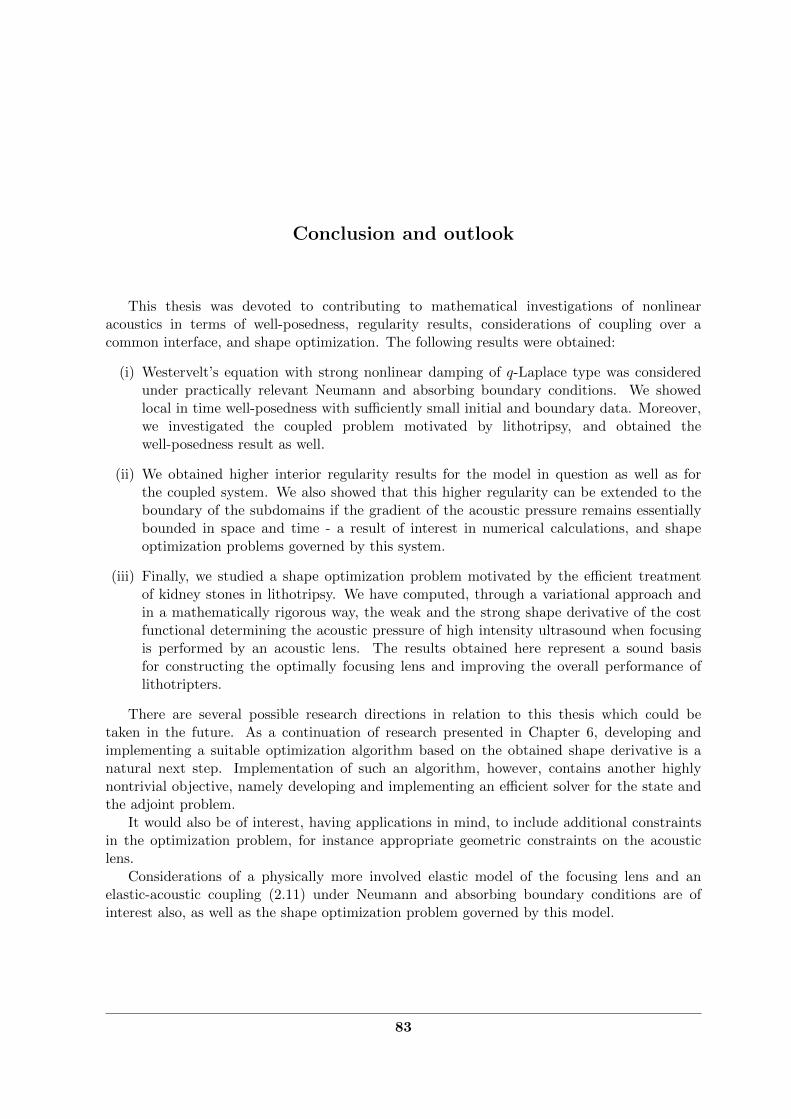
Conclusion and outlook

This thesis was devoted to contributing to mathematical investigations of nonlinearacoustics in terms of well-posedness, regularity results, considerations of coupling over acommon interface, and shape optimization. The following results were obtained:

(i) Westervelt’s equation with strong nonlinear damping of q-Laplace type was consideredunder practically relevant Neumann and absorbing boundary conditions. We showedlocal in time well-posedness with sufficiently small initial and boundary data. Moreover,we investigated the coupled problem motivated by lithotripsy, and obtained thewell-posedness result as well.

(ii) We obtained higher interior regularity results for the model in question as well as forthe coupled system. We also showed that this higher regularity can be extended to theboundary of the subdomains if the gradient of the acoustic pressure remains essentiallybounded in space and time - a result of interest in numerical calculations, and shapeoptimization problems governed by this system.

(iii) Finally, we studied a shape optimization problem motivated by the efficient treatmentof kidney stones in lithotripsy. We have computed, through a variational approach andin a mathematically rigorous way, the weak and the strong shape derivative of the costfunctional determining the acoustic pressure of high intensity ultrasound when focusingis performed by an acoustic lens. The results obtained here represent a sound basisfor constructing the optimally focusing lens and improving the overall performance oflithotripters.

There are several possible research directions in relation to this thesis which could betaken in the future. As a continuation of research presented in Chapter 6, developing andimplementing a suitable optimization algorithm based on the obtained shape derivative is anatural next step. Implementation of such an algorithm, however, contains another highlynontrivial objective, namely developing and implementing an efficient solver for the state andthe adjoint problem.

It would also be of interest, having applications in mind, to include additional constraintsin the optimization problem, for instance appropriate geometric constraints on the acousticlens.

Considerations of a physically more involved elastic model of the focusing lens and anelastic-acoustic coupling (2.11) under Neumann and absorbing boundary conditions are ofinterest also, as well as the shape optimization problem governed by this model.

83

Conclusion and outlook

84

Notational convention

Physical quantities

u acoustic pressure

v acoustic particle velocity

c speed of sound

% mass density

ψ acoustic velocity potential, %ψ = u

λ bulk modulus

B/A parameter of nonlinearity

b diffusivity of sound in the Westervelt equation

with constant coefficients, see page 8, or the quotient

of the diffusivity of sound and the bulk modulus

in the coupled model, see page 38

k = 1λ(1 +B/(2A))

Sets

Ω domain in Rd, d ∈ 1, 2, 3Ω the closure of Ω

Ω+ the lens subdomain, see page 45

Ω− the fluid subdomain, see page 45

Function spaces

C l,α(Ω) space of l-times continuously differentiable functions

whose l-th partial derivatives are bounded and Holder

continuous with exponent α

C0,1(Ω) space of Lipschitz continuous functions

Lr(Ω) space of measurable functions that are r-integrable,

85


|u|Lr(Ω) :=(∫

Ω |u|r dx

)1/r, 1 ≤ r <∞

L∞(Ω) space of essentially bounded functions

|u|L∞(Ω) := ess supx∈Ω

|u(x)|

W l,r(Ω) space of all locally summable functions u : Ω→ Rsuch that for each α with |α| ≤ l, l ∈ N0, Dαu exists

and belongs to Lr(Ω),

|u|W l,r(Ω) :=(∑|α|≤l

∫Ω|Dαu|r dx

)1/r, 1 ≤ r <∞,

|u|W l,∞(Ω) :=∑|α|≤l

ess supΩ|Dαu|

C(0, T ;V ) space of continuous functions u : [0, T ]→ V with

‖u‖C(0,T ;V ) = maxt∈[0,T ]

|u(t)|V <∞

Ck(0, T ;V ) space of k time continuously differentiable functions

u : [0, T ]→ V with ‖u‖Ck(0,T ;V ) =

k∑j=0

‖dju

dtj‖C(0,T ;V ) <∞

Lr(0, T ;V ) space of measurable functions u : [0, T ]→ V with

‖u‖Lr(0,T ;V ) = (∫ T

0 |u(t)|rV dt)1/r <∞, 1 ≤ r <∞,

‖u‖L∞(0,T ;V ) = ess sup[0,T ]

|u(t)|V <∞

W 1,r(0, T ;V ) space of measurable functions u ∈ Lr(0, T ;V )

whose weak derivative djudtj∈ Lr(0, T ;V ), 0 ≤ j ≤ l

‖u‖W l,r(0,T ;V ) :=( k∑j=0

‖dju

dtj‖rLr(0,T ;V )

)1/r,

1 ≤ r <∞,

‖u‖W l,∞(0,T ;V ) :=∑k

j=0 ‖djudtj‖L∞(0,T ;V )

Operators

˙ first derivative with respect to the time variable

¨ second derivative with respect to the time variable

Dlr r-th difference quotient of size l, see page 41

trΓ trace operator, see page 14

∇ spatial gradient: ∇u := ( ∂u∂x1, . . . , ∂u∂xd )

∇Γ tangential gradient on Γ

div, ∇· divergence with respect to the spatial variables

86

∆ Laplace operator: ∆u := div(∇u)

∆q q-Laplace operator: ∆qu := div(|∇u|q−1∇u), q ≥ 1

Constants

C,C generic positive constants

Cq positive constant depending only on q

Ctr1 norm of the trace mapping trΓ : W 1,q+1(Ω)→W1− 1

q+1,q+1

(Γ)

Ctr2 norm of the trace mapping trΓ : H1(Ω)→ H−1/2(Γ)

CΩX,Y norm of the embedding operator X(Ω)→ Y (Ω)

between two function spaces over the domain Ω

CP constant appearing in Poincare’s inequality, see page 16

CΩ1 = |Ω|−

qq+1 , see page 16

CΩ2 = |Ω|−

q−12(q+1) , see page 16

C(ε, r) = (r − 1)rrr−1 ε−

11−r , constant appearing in Young’s

inequality, see page 17

Notation related to

shape optimization

ud the desired acoustic pressure

Oad set of admissible shapes, see page ??

χΩ+ characteristic function of Ω+

Char(Ω) set of characteristic functions

p the adjoint state

τ artificial time variable indicating varying subdomains

h vector field over the domain Ω

Fτ transformations of Ω into Rd

DFτ Jacobian of Fτ

Aτ = (DFτ )−T

Iτ = det(DFτ )

dJ(u,Ω+)h Eulerian derivative at Ω+ in the direction of the vector field h

87


88

Bibliography

[1] R. Adams and J. Fournier, Sobolev spaces, 2nd edn, Academic Press, Amsterdam, 2003.

[2] N. D. Alikakos and L. C. Evans, Continuity of the gradient for weak solutions of adegenerate parabolic equation, Journal de Mathematiques Pures et Appliquees, vol. 62,issue 3, 253–268, 1983.

[3] H. Ammari, D. Chen, and J. Zou, Well-posedness of a pulsed electric field model inbiological media and its finite element approximation, arXiv:1502.06803v2 [math.AP].

[4] K. Atkinson and W. Han, Theoretical numerical analysis, 3rd edn, Springer, 2009.

[5] A. Bamberger, R. Glowinski, and Q. H. Tran, A domain decomposition method for theacoustic wave equation with discontinuous coefficients and grid change, SIAM Journal onNumerical Analysis, vol. 34, issue 2, 603–639, 1997.

[6] J. Barrett and W. Liu, Finite element approximation of the p-Laplacian, Mathematics ofComputation, vol. 61, issue 204, 523–537, 1993.

[7] J. Barrett and W. Liu, Finite element approximation of the parabolic p-Laplacian, SIAMJournal on Numerical Analysis, vol. 31, issue 2, 413–328, 1994.

[8] M. Berggren, A unified discrete-continuous sensitivity analysis method for shapeoptimization, Lecture at the Radon Institut, Linz, Austria, 2005.

[9] R. Brunnhuber, B. Kaltenbacher, and P. Radu, Relaxation of regularity for the Westerveltequation by nonlinear damping with application in acoustic-acoustic and elastic-acousticcoupling, Evolution Equations and Control Theory, vol. 3, issue 4, 595–626, 2014.

[10] D. Bucur and P. Trebeschi, Shape optimization problems governed by nonlinear stateequations, Proceedings of The Royal Society of Edinburgh Section A-mathematics, vol.128, issue 5, 945–963, 1998.

[11] G. Butazzo and A. Nayam, Stationary configuration of some optimal shaping, InternationalJournal of Dynamical Systems and Differential Equations, vol. 4, issue 3, 198–214, 2013.

[12] D. G. Crighton, Model equations of nonlinear acoustics, Annual Review of FluidMechanics, vol. 11, issue 1, 11–33, 1979.

[13] F. Coulouvrat, On the equations of nonlinear acoustics, Journal de Acoustique, vol. 5,321–359, 1992.

[14] M. C. Delfour and J.-P. Zolesio, Shapes and geometries, 2nd edn, SIAM, 2001.

89

Bibliography

[15] F. Demengel, G. Demengel, and R. Erne, Functional spaces for the theory of elliptic partialdifferential equations, Springer, 2012.

[16] E. DiBenedetto, Degenerate parabolic equations, Springer Science & Business Media, 2012.

[17] J. Douglas and T. Dupont, A Galerkin method for a nonlinear Dirichlet problem,Mathematics of Computation, vol. 29, issue 131, 689–696, 1975.

[18] T. Dreyer, W. Kraus, E. Bauer, and R. E. Riedlinger, Investigations of compact focusingtransducers using stacked piezoelectric elements for strong sound pulses in therapy,Proceedings of the IEEE Ultrasonics Symposium, 1239–1242, 2000.

[19] D. Ensminger and F. Stulen, Ultrasonics: data, equations, and their practical uses, CRCPress (Taylor & Francis Group), 2009.

[20] L. C. Evans, Partial Differential Equations, 2nd edn, American Mathematical Society,Providence, 1998.

[21] E. DiBenedetto and A. Friedman, Regularity of solutions of nonlinear degenerate parabolicsystems, Journal fur die reine und angewandte Mathematik, vol. 349, 83–128, 1984.

[22] A. Farina, B. Sciunzi, and E. Valdinoci, Bernstein and De Giorgi type problems: Newresults via a geometric approach, Annali della Scuola Normale Superiore di Pisa–Classe diScienze, vol. 7, issue 4, 741–791, 2008.

[23] P. Grisvard, Elliptic problems in nonsmooth domains, Monographs and Studies inMathematics, vol. 24, Pitman, Massachusetts, 1985.

[24] P. Gangl, U. Langer, A. Laurain, H. Meftahi, and K. Sturm, Shape optimization of anelectric motor subject to nonlinear magnetostatics, arXiv:1501.04752v1 [math.OC].

[25] H. Gao and T. F. Ma, Global solutions for a nonlinear wave equation with the p−Laplacianoperator, Electronic Journal of Qualitative Theory of Differential Equations, vol. 11, 1–13,1999.

[26] M. F. Hamilton and D. T. Blackstock, Nonlinear Acoustics, Academic Press, New York,1997.

[27] R. Hiptmair, A. Paganini, and S. Sargheini, Comparison of approximate shape gradients,BIT Numerical Mathematics, vol. 55, issue 2, 459–485, 2014.

[28] S. Hofmann, M. Mitrea, and M. Taylor, Geometric and transformational properties ofLipschitz domains, Semmes-Kenig-Toro Domains, and other classes of finite perimeterdomains, The Journal of Geometric Analysis, vol. 17, issue 4, 593–647, 2007.

[29] K. Ito, K. Kunisch, and G. Peichl, Variational approach to shape derivatives for a class ofBernoulli problems, Journal of Mathematical Analysis and Applications, vol. 314, issue 1,126–149, 2006.

[30] K. Ito, K. Kunisch, and G. Peichl, Variational approach to shape derivatives, ESAIM:Control, Optimisation and Calculus of Variations, vol. 14, issue 3, 517–539, 2008.

90

Bibliography

[31] X. Q. Jian, L. S. Wu, Zh. H. Li, W. L. Li, and J. G. Yin, Temperature fieldFDTD simulation of HIFU in human body tissues, The 2nd International Conference onBioinformatics and Biomedical Engineering, 759–762, 2008.

[32] P. M. Jordan, An analytical study of Kuznetsov’s equation: diffusive solutions, shockformation, and solution bifurcation, Physics Letters A, vol. 326, issue 1, 77–84, 2004.

[33] B. Kaltenbacher, Boundary observability and stabilization for Westervelt type waveequations without interior damping, Applied Mathematics and Optimization, vol. 62, issue3, 381–410, 2010.

[34] B. Kaltenbacher and I. Lasiecka, Global existence and exponential decay rates for theWestervelt equation, Discrete and Continuous Dynamical Systems Series S, vol. 2, issue 3,503–525, 2009.

[35] B. Kaltenbacher and I. Lasiecka, Well-posedness of the Westervelt and the Kuznetsovequation with nonhomogeneous Neumann boundary conditions, AIMS Proceedings,763–773, 2011.

[36] B. Kaltenbacher, I. Lasiecka, and S. Veljovic, Well-posedness and exponential decay for theWestervelt equation with inhomogeneous Dirichlet boundary data, Progress in NonlinearDifferential Equations and Their Applications, vol. 60, 357–387, 2011.

[37] B. Kaltenbacher and G. Peichl, Sensitivity analysis for a shape optimization problem inlithotripsy, in preparation.

[38] B. Kaltenbacher and S. Veljovic, Sensitivity analysis of linear and nonlinear lithotriptermodels, European Journal of Applied Mathematics, vol. 22, issue 1, 21–43, 2010.

[39] M. Kaltenbacher, Numerical simulations of mechatronic sensors and actuators, Springer,Berlin, 2004.

[40] M. Kaltenbacher, H. Landes, J. Hoffelner, and R. Simkovics, Use of modern simulationfor industrial applications of high power ultrasonics, Proceedings of the IEEE UltrasonicsSymposium, CD-ROM Proceedings, 673–678, 2002.

[41] H. Kasumba and K. Kunisch, Vortex control in channel flows using translational invariantcost functionals, Computational Optimization and Applications, vol. 52, issue 3, 691–717,2012.

[42] V. P. Kuznetsov, Equations of nonlinear acoustics, Soviet Physics Acoustics, vol. 16, issue4, 467–470, 1971.

[43] A. Laurain and K. Sturm, Domain expression of the shape gradient and application toelectrical impedance tomography, Technical Report 1863, Weierstrass Institute for AppliedAnalysis and Stochastics, 2013.

[44] G. Leoni, A first course in Sobolev spaces, American Mathematical Society, Providence,2009.

[45] G. M. Lieberman, Boundary regularity for solutions of degenerate elliptic equations,Nonlinear Analysis: Theory, Methods & Applications, vol. 12, issue 11, 1203–1219, 1988.

91

Bibliography

[46] P. Lindqvist, Notes on p-Laplace equation, Lecture notes, University of Jyvaskyla, 2006.

[47] W. Liu and N. Yan, Quasi-norm local error estimators for p-Laplacian, SIAM Journal onNumerical Analysis, vol. 39, issue 1, 100–127, 2002.

[48] F. Murat and J. Simon, Sur le controle par un domaine geometrique, Rapport 76015,Universite Pierre et Marie Curie, Paris, 1976.

[49] S. Makarov and M. Ochmann, Nonlinear and thermoviscous phenomena in acoustics, PartII, Acta Acustica united with Acustica, vol. 83, issue 2, 197–222, 1997.

[50] A. Neisius, N. B. Smith, G. Sankin, N. J. Kuntz, J. F. Madden, D. E. Fovargue, S. Mitran,M. E. Lipkin, W. N. Simmons, G. M. Preminger, and P. Zhong, Improving the lens designand performance of a contemporary electromagnetic shock wave lithotripter, Proceedingsof the National Academy of Sciences, vol. 111, issue 13, 1167–1175, 2014.

[51] V. Nikolic, Local existence results for the Westervelt equation with nonlinear damping andNeumann as well as absorbing boundary conditions, Journal of Mathematical Analysis andApplications, vol. 427, issue 2, 1131–1167, 2015.

[52] V. Nikolic and B. Kaltenbacher, On higher regularity for the Westervelt equation withstrong nonlinear damping, arXiv:1506.02125 [math.AP], and submitted.

[53] V. Nikolic and B. Kaltenbacher, Sensitivity analysis for shape optimization of a focusingacoustic lens in lithotripsy, arXiv:1506.02781 [math.AP], and submitted.

[54] M. A. Rammaha and Z. Wilstein, Hadamard well-posedness for wave equations withp-Laplace damping and supercritical sources, Advances in Differential Equations, vol. 17,issue 1/2, 105–150, 2012.

[55] T. Roubıcek, Nonlinear partial differential equations with applications, Birkhauser Basel,2005.

[56] J. Sokolowski and J.-P. Zolesio, Introduction to shape optimization, Springer, Berlin, 1991.

[57] V. Schulz, M. Siebenborn, and K. Welker, A novel Steklov-Poincar type metric for efficientPDE constrained optimization in shape spaces, arXiv:1506.02244v4 [math.OC].

[58] S. Tjøtta, Higher order model equations in nonlinear acoustics, Acta Acustica united withAcustica, vol. 87, issue 3, 316–321, 2001.

[59] F. Troltzsch, Optimal control of partial differential equations: theory, methods andapplications, AMS 2010 Graduate Studies in Mathematics, 2010.

[60] N. N. Ural’tseva, Degenerate quasilinear elliptic systems, Zap. Na. Sem. Leningrad. Otdel.Mat. Inst. Steklov. (LOMI), vol. 7, 184–222, 1968.

[61] S. Veljovic, Shape optimization and optimal boundary control for high intensity focusedultrasound (HIFU), PhD thesis, University of Erlangen-Nuremberg, 2009.

[62] D. Wei and P. Jordan, A note on acoustic propagation in power-law fluids: Compactkinks, mild discontinuities, and a connection to finite-scale theory, International Journalof Non-Linear Mechanics, vol. 48, 72–77, 2013.

92

Bibliography

[63] P. J. Westervelt, Parametric acoustic array, The Journal of the Acoustic Society ofAmerica, vol. 35, issue 4, 535–537, 1963.

[64] Z. Wilstein, Global well-posedness for a nonlinear wave equation with p-Laplacian damping,PhD thesis, University of Nebraska-Lincoln, 2011.

[65] F. Wu, Z.-B. Wang, Y.-D. Cao, W.-Z. Chen, J. Bai, J.-Z. Zou, and H. Zhu, A randomisedclinical trial of high-intensity focused ultrasound ablation for the treatment of patients withlocalised breast cancer, British Journal of Cancer 89, vol. 12, 2227–2233, 2003.

[66] F. Wu, Z.-B. Wang, H. Zhu, W.-Z. Chen, J.-Z. Zou, J. Bai, K.-Q. Li, C.-B. Jin, F.-L.Xie, and H.-B. Su, Feasibility of US-guided high-intensity focused ultrasound treatment inpatients with advanced pancreatic cancer: initial experience, Radiology, vol. 236, issue 3,1034–1040, 2005.

[67] S. Zhu, T. Dreyer, M. Liebler, R. Riedlinger, G. M. Preminger, and P. Zhong, Reduction oftissue injury in shock-wave lithotripsy by using an acoustic diode, Ultrasound in Medicine& Biology, vol. 30, issue 5, 675–682, 2004.

93

Bibliography

94

Index

C l,1-diffeomorphism, 13q-Laplacian, 9

boundary conditionsabsorbing, 20Dirichlet, 19Neumann, 20

contractivity, 36, 51cost functional, 53coupling

acoustic-acoustic, 11elastic-acoustic, 11

difference quotient, 41integration by parts formula, 41the product rule, 41

domainsC l,1-regular, 13Lipschitz regular, 13

embeddingscompact, 14continuous, 14

energy estimate, 22, 28Eulerian derivative, 59

Galerkin’s method, 23

inequalityPoincare’s , 16involving q-Laplacian, 17Young’s, 17

initial-value problemDirichlet boundary conditions, 19, 38Neumann and absorbing boundary

conditions, 20, 39

perturbation of the identity, 58

self-mapping, 35, 51shape derivative

strong, 82weak, 76

shape differentiable, 59straightening out the boundary, 47

tangential gradient, 80theorem

Banach’s fixed point, 15Bolzano-Weierstrass, 15Lebesgue dominated convergence, 15Structure, 60

Westervelt’s equation, 8with strong nonlinear damping, 9

95

On certain mathematical aspects of nonlinear acoustics ... · Fluid g. 1.1: Schematic of a power...

Documents

Transcript of On certain mathematical aspects of nonlinear acoustics ... · Fluid g. 1.1: Schematic of a power...