SLAC-PUB-12505

May 2007

On Biology as an Emergent Science

H. Pierre Noyes ∗

Stanford Linear Accelerator Center

Stanford University, Stanford, CA 94309

Abstract

Biology is considered here as an “emergent science” in the sense of Anderson

and of Laughlin and Pines. It is demonstrated that a straightforward mathematical

definition of “biological system” is useful in showing how biology differs in structure

from the lower levels in Anderson’s “More is Different” hierarchy. Using cells in

a chemostat as a paradigmatic exemplar of a biological system, it is found that a

coherent collection of metabolic pathways through a single cell in the chemostat also

satisfies the proposed definition of a biological system. This provides a theoretical and

mathematical underpinning for Young’s fundamental model of biological organization

and integration. Evidence for the therapeutic efficacy of Young’s method of analysis

is provided by preliminary results of clinical trials of a specific application of Young’s

model to the treatment of cancer cachexia.

A preliminary version of this paper, entitled “On Emergent Science”,

was presented at the 28th Annual Meeting of the Alternative Natural

Philosophy Association, Wesley House, Jesus Lane, Cambridge, England,

August 2006. This version will appear in the Proceedings of that meeting.

∗Work supported in part by Department of Energy contract DE–AC02–76SF00515.

Invited talk presented at 28th Annual Meeting Of The Alternative Natural Philosophy Association,

8/4/2006-8/8/2006, Cambridge, England

1 Why “Emergent Science”?

1.1 Anderson, and Laughlin and Pines on “emergence”

In a famous paper Anderson[1] has pointed out that there is a natural hierarchy of

scientific ideas. He starts with the usual (reductionist) strategy of the search for

the laws obeyed by the elementary entities of physics, but then points out that the

possibility of reduction does not imply constructivity. Rather, if science Y underlies

some science X: “The elementary entities of science X obey the laws of science

Y ”. The Y → X hierarchy Anderson proposes is: elementary particle physics →solid state or many body physics; many body physics → chemistry; chemistry →molecular biology; molecular biology → cell biology; .... ; physiology → psychology;

psychology → social sciences. Anderson goes on to state that “... this hierarchy does

not imply that science X is ‘just applied Y’. At each stage entirely new laws, concepts

and generalizations are necessary, requiring inspiration and creativity to just as great

a degree as in the previous one.” I heartily agree!

Although my conventional scientific career (in elementary particle physics) started

out with the conventional scientific (reductionist) assumption that the only way to

solve a basic scientific problem was to find the elementary entities, the laws they obey,

and then construct higher levels of science from that basis, I now realize that I was

mistaken. I have become convinced that 21st century science will be most exciting

and fruitful if its basic problem is taken to be not only to find out if there are general

hierarchy bridging laws that connect each level to the next and lead to novel types

of complexity, but also if there are bridging laws which overarch the “elementary”

bridging connection. This is one message I read into the paper on emergent science

by Laughlin and Pines[2] who explicitly start from Anderson’s analysis. Laughlin’s

book[3] is criticized by Leggett[4] under the title “Emergence Is in the Eye of the

Beholder.” However, I am still particularly impressed by the fact that the values

of hc/2e and e2/h obtained by electric measurements in complex systems can be

obtained to much higher accuracy than the values which can be obtained by direct

“elementary particle” measurements, despite the fact that the details of the theories

2

used to understand the complex systems providing the data for these results have not

reached consensus agreement.

1.2 The Organizing Principle of Darwinian Biology

Laughlin and Pines[2] also note that “For the biologist, evolution and emergence

are part of daily life.” As Fred Young remarked when I started discussing emergent

science with him, “Everything I ever said at ANPA (cf.[5]) was in the direction of

emergent science”. This was sure to catch my attention because for several years Fred

Young[6] has been trying to explain to me how his thesis work[7] is becoming more

and more important for him as an explanatory tool of use in understanding how recent

metabolic and physiological research all fits together. When James Lindesay joined

these discussions of Fred’s work, our joint understanding began to take shape as a

paper[8]. Briefly, I saw that Young’s results and Lindesay’s mathematical deduction

from them could be interpreted as the starting point for adding the links “cell biology

↔ biological systems ↔ ecological systems and evolutionary biology” to Anderson’s

proposed hierarchy in a specific way.

The careful reader will note that — in contrast to the earlier steps in Anderson’s

hierarchy — I have used the symbol “↔” for the connective between levels of the

hierarchy once biology enters the picture. The symbol “→” used by Anderson is

an irreversible transition which replaces the “elementary particles” of the lower level

by the laws they obey as the “elementary entities” of the new phenomena which

occur at the more complex (higher) level, and which require the invention of new

organizing principles, etc. which “emerge” from the careful study of this richer world

of ideas. Biology arrived at its fundamental organizing principle by another route.

Some biologists did not even believe that the phenomena they studied obeyed all

of the laws of physics, in particular the second law of thermodynamics! Further, it

was found useful to ask what purpose a particular aspect of these complex biological

systems had “evolved” to satisfy. This kind of teleological explanation had been

banished from physics after a very hard struggle, but its pragmatic usefulness in

biology is hard to deny. That a “higher level” organizing principle can in fact lead

3

to deductive and demonstrable conclusions when applied “top down” to a lower level

biological entity is one of the points I wish to make below. This is why I replace

“→” by “↔” in the hierarchy once we enter the biological realm. Of course I must

avoid the traps that lead to error when teleological reasoning is used carelessly. I

hope the reader will reserve judgment as to whether I succeed in doing this until my

methodology is presented clearly. In particular I believe that my methodology also

avoids the traps pointed out by Anderson and by Laughlin and Pines, with whose

basic conclusions I do agree.

Biology has sometimes been called a “Baconian” science in the sense that it started

by amassing all kinds of details and facts assumed to be relevant to the subject

and then induced general rules governing these facts. This methodology is to be

contrasted with the tradition in the “mathematical” sciences which started from the

astronomical practice of using numerical and geometrical models to make testable

predictions. Skipping over vital historical details, this had the historical result that

the “physical sciences” came to rely primarily on reductionism and hypothetical-

deductive methodology for testing. Chemistry started out as a Baconian science, but

began making the transition to a physical science in the nineteenth century thanks

to electro-chemistry, thermodynamics and statistical mechanics. Quantum mechanics

more or less allowed that transition to be completed; this transition has often been

used as the leading example of the triumph of the reductive-hypothetical-deductive

methodology.

Biology has not as yet made much fundamental use of mathematics. Its greatest

nineteenth century success was the explanation of evolution via Malthus’ observation

that (in a stable environment and over a sufficient period of time) a persistent pop-

ulation must have birthrate = deathrate. Starting from that deduction and with

observations (in particular Darwin’s) of descent with modification, Darwin and in-

dependently Wallace came to the conclusion that “evolution by natural selection” is

inevitable. This was the non-quantitative starting point for a scientific “evolution-

ary biology”. Since then this has remained unshaken as the organizing principle of

scientific biology. Clearly — if my description of the history is roughly correct —

this is a very different route to a basic organizing principle than the routes followed

4

in those “physical sciences” which now rest on hypothetical-deductive mathematical

foundations.

One qualitative fact about biology which makes a methodological difference be-

tween it and the physical sciences is that “natural selection” inevitably presupposes

the existence of some sort of environment within which the biological systems evolve,

making it logically impossible to discuss biological systems without considering their

interaction with that environment. I make explicit use of this fact in my definition of

what is meant by a “biological system” in the sub-section which follows. A corollary

of this point of view is that the paradigm of most importance in getting the study of

biology off the ground is a persistent, evolved system. We will see that this provides

a reference state, allowing fluctuations away from that reference state to be studied

quantitatively.

1.3 A Proposed Mathematical Definition of a Biological sys-

tem

I define a persistent biological system B as a finite, countable population of individual

constituents CB which in a suitable environment at constant temperature and pres-

sure is a throughput (of molecules), steady state system satisfying the first and second

laws of thermodynamics. The environment must supply food and fuel (F ) at a rate

sufficient to maintain the steady state. B acts catalytically to convert the food and

fuel into product molecules P which are retained by the individual living constituents

and waste molecules W which are disposed of by the environment. The environment

must also remove the waste heat required by the second law in such a way as to

maintain the postulated constant temperature and pressure. The environment must

remove that selection of living individual constituents whose disposal will maintain

within the system (on average) a constant distribution of living constituents over all

the states which can occur during the lifetime of any of them. The environment must

absorb all dead constituents. This implies that “dead constituents” become part of

the environment “at death”and are no longer part of B. In our context the (average)

5

number of (living) constituents satisfy the growth rate equation

CB = kBCB (1)

and are said to be in a state of stable population (SP).

Note that CB is a “counting number”. As such, it is necessarily dimensionless in

terms of a physicist’s dimensional units of mass, length and time “M,L, T”. Then

CB and kB each have the dimension of inverse time (T−1). By taking Eq. 1 as our

defining equation for biology (in the context of a SP reference state), we emphasize

in a different way the importance of the environment in our definition of biology.

Lacking any evidence for a persistent physical environment, any biological system

satisfying our definition — let alone its individual constituents — must have a finite

lifetime.

2 The Young Model for the Organization and In-

tegration of Biological Systems

2.1 The Chemostat as Paradigm for a Biological System

Our definition of product molecules P given in Sec. 1.3 allows us to specify the

distribution of living constituents by the (average) number of product molecules they

contain at any stage during the life cycle of each constituent. We illustrate how this

can be done by narrowing the specific paradigm for a biological system used here

to a group of cells in a chemostat maintained in a SP state. For the purposes of

our theoretical analysis we assume that we can treat each cell in the chemostat as a

coherent combination of its chemical constituents. Then we can use the symbol “CB”

to stand for a molecule in the chemist’s sense†. This allows us to write chemical

equations (conserving the numbers of each type of atom and the sum of their masses)

†A chemist’s “molecule” is a coherent structure which contains one or more chemical “atoms”,

while a physicist usually thinks of an “atom” as composed of still more elementary constituents, and

of a “molecule” as composed of two or more atoms.

6

connecting individual molecules to cells, which we take to be one of the (implicit)

axioms of biochemistry.

We are now dealing with a population of growing cells inside the chemostat ab-

sorbing nutrient molecules F and producing product molecules P which are retained

by the cell and waste molecules W which are excreted into the solution surrounding

the cell. Since the cell eventually divides into two cells which — at our level of anal-

ysis — are indistinguishable, we index the growing cells by the number of product

molecules nP they have added in the range NP ≤ nP ≤ 2NP −1. Cell division is then

the irreversible process

CB(2NP ) ⇒ 2CB(NP ) (2)

The basic biochemical process in this context is

F + CB(NP + nP ) ⇒ CB(NP + nP + 1) + W (3)

Consequently the chemical equation describing the operation of the chemostat in this

simplest case is

NF F + Σ2NP−1nP =0 CB(NP + nP ) ⇒ Σ2NP−1

nP =1 CB(NP + nP ) + 2CB(NP ) + NW W (4)

which, by defining a complete population of cells (i.e. a population which, in the

appropriate environmental context, when supplied with NF nutrient molecules, can

produce two clones by cell division) as ΣCB ≡ Σ2NP−1nP =0 CB(NP + nP ), we can rewrite

as

NF F + ΣCB ⇒ ΣCB + CB(NP ) + NW W (5)

or as

NF F⇒

ΣCBCB(NP ) + NW W (6)

A growing cell has to add NP product molecules to its structure before it can divide

and start the process over again. One of those two copies (clones) must be removed

7

at some subsequent time (in its life cycle or when it dies); this pruning is required

to maintain the SP state. In this particulate description of the overall process, any

growing cell will have to add each individual product molecule sequentially. We

assume that the context in which the equations apply is a through-put steady state

(SP state). Then the rate at which the molecules of F move into the growing cell,

the rate at which the molecules of P join the growing cell, the rate at which the

cell divides into two clones (beginning cells), and the rate at which one of these two

growing cells is eventually pruned from the cell colony are all the same. That is

[CB] = kB[CB]; [F ] = kB[F ]; [P ] = kB[P ]; [W ] = kB[W ] (7)

Here the symbol [X] (X ∈ CB, F, P, W ) means the concentration (i.e mass per unit

volume) of the substance X, For small molecules (i.e. molecules whose atomic content

and (if needed) molecular structure are known) this mass is most conveniently mea-

sured in terms of moles (i.e. gram molecular weights). These equations immediately

suggest that it may be possible to treat concentrations of small molecules as biological

systems in an appropriate context. We develop this idea in the next sub-section, in

which we give precision to the concept of metabolic pathway.

The careful reader will have noted that we have use the symbol ⇒ denoting the

irreversibility of the chemical reaction not only for cell-division (Eq. 2) but also for the

individual step (Eq. 3) in which the cellular environment catalyzes the transition from

food molecule(s) to the product and waste molecules. We assume that this can only

happen when the initial and final molecules are in the correct stoichiometric ratios

(see next section). This is because we are interested in this paper only in the passage

of molecules through the cell (or to their location within the cell) when this path does

go through some catalytic site (which we will call an enzyme) that guarantees that we

are talking about a throughput steady state which is far from equilibrium and not

about the equilibrium states with which much of physical chemistry is concerned.

Thus there are no two-way transitions at the basic level and the usual use of detailed

balance rate constants is, from the start, inapplicable. This brings us to the discussion

of (enzymatic) metabolic pathways in the next section.

8

2.2 A Coherent Collection of Metabolic Pathways as a Paradigm

for a Biological System

The food/fuel molecule or molecules F that initiate the basic process (Eq. 3) could

have entered the cell at many different places, and the waste molecule or molecules

that complete the process can leave the cell at many different places, but (in our

abstract model) the critical transition occurs at only one place along the path(s)

connecting the input and output surface patches, namely where some enzyme EF⇒PW

catalyzes the reaction hF F ⇒ hP P + hW W . We call this “one dimensional” route

through the cell a metabolic pathway and represent its action by the biochemical

equation

E · hF F

↗ ↘

hF F + E E + hP P + hW W (8)

↖ ↙

E

Eq. 8 represents the irreversible, catalytic action of a single enzyme molecule,

which may dynamically change its shape during the process but automatically re-

sumes its initial shape after the process is completed‡. Note that, for the biochemical

processes used in our paradigm, this process must occupy a (3+1)-dimensional space-

time volume and hence must be nonlocal. The numbers hF , hP and hW must be

integers because both the number of (chemical) atoms and the amount of (chemical)

mass are conserved in the process. Their ratios hX/Y ≡ hX/hY = (hY /hX)−1 =

h−1Y/X ; X, Y ∈ F, P, W, ... are called stoichiometric ratios. If we measure the concen-

tration [X] [which has physical dimensions ML−3 (i.e mass per unit volume)] of any

chemical substance X in moles (i.e. in gram-molecular weights per unit volume), then

‡This restoration of the initial state of the enzyme provides one “feedback” control mechanism.

Some feedback control loop in the information flow is required for any persistent, self-organizing

complex system to exist.

9

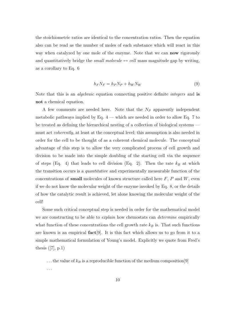
the stoichiometric ratios are identical to the concentration ratios. Then the equation

also can be read as the number of moles of each substance which will react in this

way when catalyzed by one mole of the enzyme. Note that we can now rigorously

and quantitatively bridge the small molecule ↔ cell mass magnitude gap by writing,

as a corollary to Eq. 6

hF NF = hP NP + hW NW (9)

Note that this is an algebraic equation connecting positive definite integers and is

not a chemical equation.

A few comments are needed here. Note that the NP apparently independent

metabolic pathways implied by Eq. 4 — which are needed in order to allow Eq. 7 to

be treated as defining the hierarchical nesting of a collection of biological systems —

must act coherently, at least at the conceptual level; this assumption is also needed in

order for the cell to be thought of as a coherent chemical molecule. The conceptual

advantage of this step is to allow the very complicated process of cell growth and

division to be made into the simple doubling of the starting cell via the sequence

of steps (Eq. 4) that leads to cell division (Eq. 2). Then the rate kB at which

the transition occurs is a quantitative and experimentally measurable function of the

concentrations of small molecules of known structure called here F , P and W , even

if we do not know the molecular weight of the enzyme invoked by Eq. 8, or the details

of how the catalytic result is achieved, let alone knowing the molecular weight of the

cell!

Some such critical conceptual step is needed in order for the mathematical model

we are constructing to be able to explain how chemostats can determine empirically

what function of these concentrations the cell growth rate kB is. That such functions

are known is an empirical fact[9]. It is this fact which allows us to go from it to a

simple mathematical formulation of Young’s model. Explicitly we quote from Fred’s

thesis ([7], p.1)

. . . the value of kB is a reproducible function of the medium composition[9]

. . .

10

which we write formally as

kB = KB([F1], [F2], ..., [Fj], ..., [FJ ]) (10)

Here the nutrients Fj are distinguished from each other by the unique enzymes Ej

which catalyze the irreversible reactions

hFjFj

⇒Ej

hPjPj + hWj

Wj (11)

that remove hFjmolecules of Fj from the metabolic pathway and replaces them with

product (Pj) and waste (Wj) molecules, conserving chemical mass and atom flux. J

is the number of types of enzymes and the number of types of metabolic pathways

we consider important in any particular analysis. KB is not a function in the usual

mathematical sense. For us, if the values of the parameters are known over the ranges

of values and to the accuracy needed for our immediate purposes, a “table lookup”

plus any well defined “interpolation procedure” suffice to make this framework into

a testable theory in Popper’s sense.

Accepting that Eq. 10 is a reproducible empirical statement based on table lookup

has important consequences. In that context the inescapable fact is that all the

numerical quantities (in this case kB and each of the [Fj]) have an experimental

range of uncertainty. I formalize this fact by assuming that whenever we assert Eq.

10, we are claiming that there are 2(J + 1) numbers called kmin, kmax, [Fj]min, [Fj]max

such that for any choice of numerical values within these ranges, no matter how

correlated, the asserted equality provides an acceptable representation of the data

for our purposes. If this statement becomes suspicious, the careful experimenter will

look for an explanation either in some source of systematic error, or some theoretical

constraint or possibility that has been ignored. Note that in either case, these limits

become testable hypotheses in Popper’s sense, and new experiments can either reduce

the experimental uncertainty or produce new empirical knowledge. This is standard

procedure in physics.

With this understood, we can use some hypothesis that makes nutrient “j” the

“most important” for the purposes of our analysis, and formally “invert” Eq.10 by

11

defining

[Fj] = (KB)−1j (kB; [F1], [F2], ..., [Fj−1], [Fj+1], ..., [FJ ]) ≈ (KB)−1

j (kB) (12)

which means that, to the extent that the approximation is valid, we can ignore what

is going on in the concentrations of the other nutrients and find some monotonically

increasing function of kB, kmin < kB < kmax to fit the observed values of the correlated

variation of [Fj], for [Fj]min < [Fj] < [Fj]max (or visa versa), — i.e. kB = (KB)j([Fj]).

With this basic phenomenology understood we can make testable empirical hypothe-

ses about and place reasonable theoretical constraints on the concept of “metabolic

pathway” in the context of a stable population of bacterial cells in a chemostat.

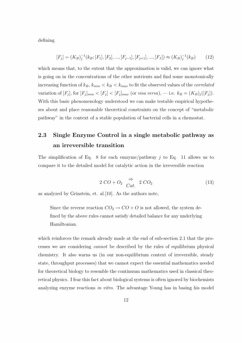
2.3 Single Enzyme Control in a single metabolic pathway as

an irreversible transition

The simplification of Eq. 8 for each emzyme/pathway j to Eq. 11 allows us to

compare it to the detailed model for catalytic action in the irreversible reaction

2 CO + O2⇒

Cat.2 CO2 (13)

as analyzed by Grinstein, et. al.[10]. As the authors note,

Since the reverse reaction CO2 → CO + O is not allowed, the system de-

fined by the above rules cannot satisfy detailed balance for any underlying

Hamiltonian.

which reinforces the remark already made at the end of sub-section 2.1 that the pro-

cesses we are considering cannot be described by the rules of equilibrium physical

chemistry. It also warns us (in our non-equilibrium context of irreversible, steady

state, throughput processes) that we cannot expect the essential mathematics needed

for theoretical biology to resemble the continuum mathematics used in classical theo-

retical physics. I fear this fact about biological systems is often ignored by biochemists

analyzing enzyme reactions in vitro. The advantage Young has in basing his model

12

on chemostat data is that these empirical studies are, in fact, in vivo experiments.

They allow us to go directly from chemical measurements (concentrations of small

molecules) to a parameter (kB) that measures the (average) time it takes a living or-

ganism to replicate itself in an environmental context that allows a biological system

composed of such organisms to achieve a persistent steady state (SP-state).

The rules the authors[10] refer to in the quote given above describe the way

to parameterize the rates at which the incoming molecules attach to the catalytic

surface, rearrange bonds to form the product molecules of the outgoing gas, and the

rates at which the outgoing molecules detach. These details need not concern us

here, nor do the numerical methods Grinstein, et. al. are forced to use because they

lack a Hamiltonian model. What does concern us is that the catalyzed transition

2CO + O2 ⇒ 2CO2 is a worked out example analogous to the way the F molecules

come along the incoming part of the metabolic pathway to a specific enzyme and the P

and W molecules leave on the distinctly different outgoing part of the same pathway.

We could make a more detailed model of this process, but we are not required to do

so in order to achieve our results. All we need abstract from the complicated process

that goes on in the ill-defined space-time volume around the enzyme is the fact that

this transition separates the metabolic pathway into an incoming and an outgoing

part, and that it fixes the stoichiometric ratios of all the substances in this single

metabolic pathway whose mass flow is continuous through this volume.

The reason we are not concerned with the geometrical details is that the basic

equations (Eq. 7) are space-scale invariant and only depend on spacial averages

(concentrations) as functions of time. To smooth these out in the complicated region

where F attaches to the enzyme, the enzyme rearranges F into P and W and these

leave, we assume this region has an average length L. We assume that an average flow

velocity for molecules along this metabolic pathway through the cell can be defined

by v = kBL. Then within this region, we can measure distance along the pathway by

a spatial coordinate x = vt = LkBt when 0 < x < L, 0 < t < TB = k−1B . Assume that

the pathway is in an SP-state (i.e. v = const. = kBL = L/TB ). Upstream of this

transition region (i.e x < 0) the concentration [Fj] must have a constant input value

which we call [Fj]I . Downstream of the transition region the concentrations [Pj] and

13

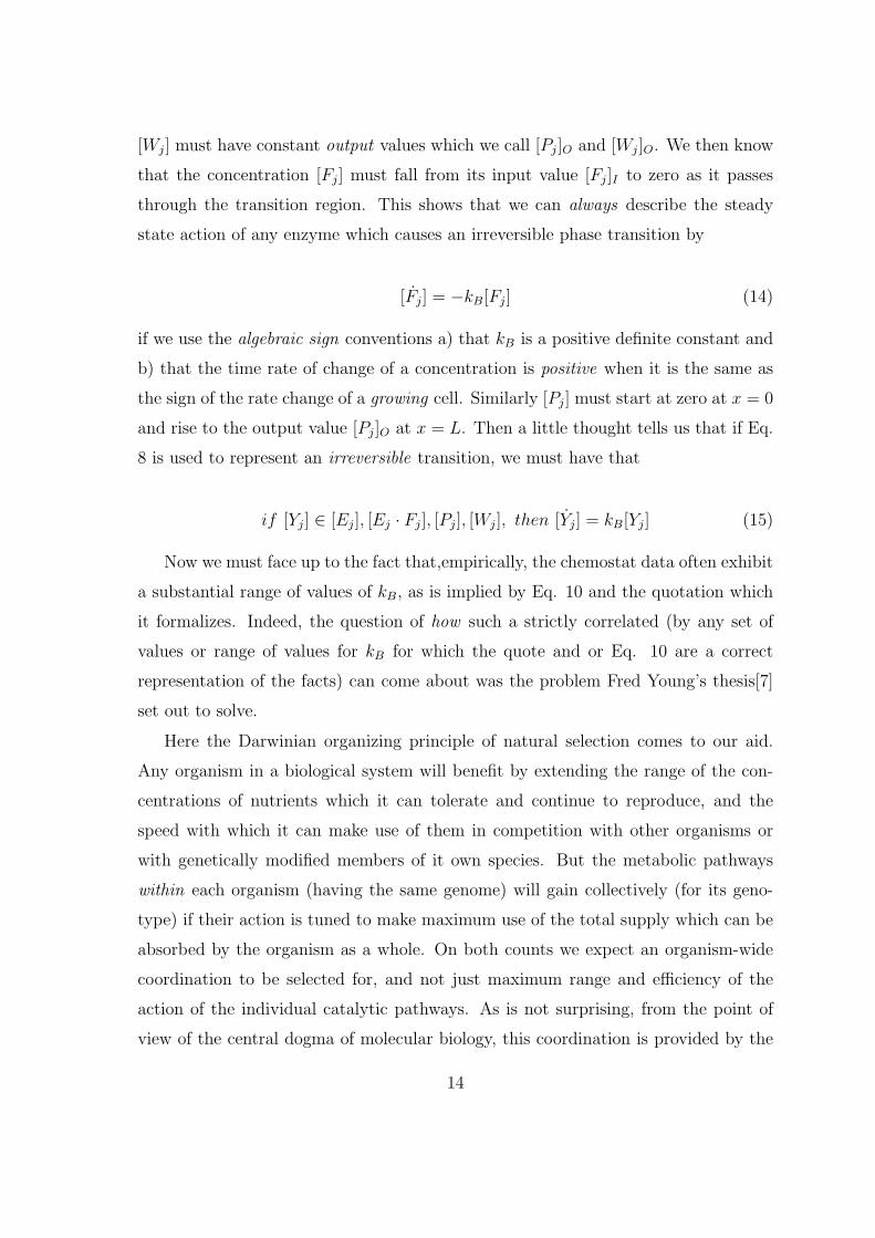
[Wj] must have constant output values which we call [Pj]O and [Wj]O. We then know

that the concentration [Fj] must fall from its input value [Fj]I to zero as it passes

through the transition region. This shows that we can always describe the steady

state action of any enzyme which causes an irreversible phase transition by

[Fj] = −kB[Fj] (14)

if we use the algebraic sign conventions a) that kB is a positive definite constant and

b) that the time rate of change of a concentration is positive when it is the same as

the sign of the rate change of a growing cell. Similarly [Pj] must start at zero at x = 0

and rise to the output value [Pj]O at x = L. Then a little thought tells us that if Eq.

8 is used to represent an irreversible transition, we must have that

if [Yj] ∈ [Ej], [Ej · Fj], [Pj], [Wj], then [Yj] = kB[Yj] (15)

Now we must face up to the fact that,empirically, the chemostat data often exhibit

a substantial range of values of kB, as is implied by Eq. 10 and the quotation which

it formalizes. Indeed, the question of how such a strictly correlated (by any set of

values or range of values for kB for which the quote and or Eq. 10 are a correct

representation of the facts) can come about was the problem Fred Young’s thesis[7]

set out to solve.

Here the Darwinian organizing principle of natural selection comes to our aid.

Any organism in a biological system will benefit by extending the range of the con-

centrations of nutrients which it can tolerate and continue to reproduce, and the

speed with which it can make use of them in competition with other organisms or

with genetically modified members of it own species. But the metabolic pathways

within each organism (having the same genome) will gain collectively (for its geno-

type) if their action is tuned to make maximum use of the total supply which can be

absorbed by the organism as a whole. On both counts we expect an organism-wide

coordination to be selected for, and not just maximum range and efficiency of the

action of the individual catalytic pathways. As is not surprising, from the point of

view of the central dogma of molecular biology, this coordination is provided by the

14

genetic control of the production of the enzymes themselves. Since this is more easily

explained by using the control mechanism discovered by Fred Young in his thesis than

by discussing a single enzyme pathway, we now turn to that explanation in the next

sub-section.

2.4 Two Enzymes linked by a feedback loop in a single metabolic

pathway

The basic feedback control loop for metabolic regulation which Fred Young[7] discov-

ered, written as a chemical equation, is

hUU

↗ ↘

hII + EI EO + HOO (16)

↖ ↙

hDD

Note that this connects two irreversible enzyme-catalyzed transformations, namely

hII + hDD⇒EI

hUU⇒EO

hDD + hOO (17)

Note that D — which is analogous to the the enzyme E in Eq. 8 (if we replace E · Fby D · I = U) — is conserved in the sense that it retains (in a SP-system) a constant

concentration. Note also that (in a SP-system) the net effect is to transform I to O

irreversibly, conserving mass and chemical atoms, at a rate

kB =[O]

[O]= − [I]

[I]=

[U ]

[U ]=

[D]

[D](18)

This is, of course, the same conclusion we reached about the action of the individual

enzymes (cf. Eq.’s 14 nd 15). This means that we can go on connecting nodes

(representing enzymes which unequivocally direct mass flow in the direction defined

by positive growth rate or, in feedback links, unequivocally in the opposite direction)

15

in a way that will never upset the SP character of the system provided the environment

is stable and we can prove that the system is stable against “normal” fluctuations in

the environment.

Further, Eq. 18 implies that [O]

[I]= −hO/I , the negative of the stoichiometric ratio

of the concentrations. Not only is the rate of decrease of I precisely equal to the

rate of increase of O (a fact we could derive directly from chemical mass and atom

conservation), but if we think of the cell as a factory for the production of O, ratios

of the stoichiometric coefficients in Eq. 16 could serve as the set-points for some

rate control system that optimizes the use of resources I to the rate at which they

are provided. This is obvious to a chemical engineer. That natural selection has

“engineered” such a system is a deduction from the Darwinian organizing principle.

Fred Young’s approach is to “reverse-engineer” the data on the concentrations

in steady state throughput experiments using what is known about the structure

and working of the cell so as to tease out how the control system operates. One

advantage of using his control cycle, rather than concentrating on the genes (and

hence the enzymes) directly, is that his control loop allows this to be done using

only the concentrations of the small molecules as the empirical starting point. As he

notes ([7], p.8): “The interrelationships between cellular components that define the

steady-state and illustrate the scope of regulation which is independent of specific

[genetic] induction-repression mechanisms have been comprehensively tabulated.”

One general mechanism for cell-wide rate control recognized by Young is the

relation between protein synthesis and ribosome synthesis when both are thought

of as a function of kB (cf. [7], Fig. 7, p.37 and related text). For a stable population

of growing cells, and a large range of values of kB, the rate of protein synthesis

(per genome equivalent of DNA) is constant, whereas the relative rate of ribosome

synthesis is a rapidly increasing function of kB. Clearly the value of kB where these

two curves cross is a “rate control set point” .

Why is this true? The proteins are manufactured by the ribosomes. The particular

protein called for is coded on an “instruction tape” (messenger ribonucleic acid —

mRNA). This tells the ribosome which of the 20 possible amino acids to attach

next onto the growing protein (polypeptide) chain. An “expressed” DNA-gene uses

16

(ignoring ambiguities in the code) one of 20 “three letter codons” (corresponding

to the 20 amino acids which can be used to make a protein chain) to provide the

information added sequentially to the mRNA instruction tape. The fact that the

concentrations of ribosomes, ribosomal nucleic acid (rRNA), mRNA and tRNA are

all proportional to kB then tells us (accepting the one gene - one enzyme doctrine and

still subtler approximations§) that we can expect the concentration of any enzyme

(a “large molecule” made up of one or more polypeptide (protein) chains) produced

by this machinery to also be proportional to kB. The fact that the (relative) rate of

protein synthesis as a function of kB is constant (in the range where it crosses the

rate of ribosome production) can be interpreted as due to the likelihood that the rate

of transcription for any of the codons that specifies any amino acid is approximately

the same as for any other codon.

The next step is to note that the amount of the enzyme synthesized is controlled

by the expression of the gene and that this, in turn, is controlled by the operator-

promoter region of the gene. These controls can be either positive (enzyme induction)

or negative (enzyme repression) and can be effected by a change in the concentration

of any appropriate small molecule or protein in the metabolic pathway upstream of

the enzyme in question, even though it is not directly involved in the I ⇒ O catalysis.

[Such a change can even “turn off” the gene completely and hence form the starting

point for a concentration threshold -controlled on-off “switch”. We will mention such

switches in the discussion of the cancer cachexia treatment, but not model them in

this paper.]

§[DNA is a shorthand for deoxyribonucleic acid, The transfer RNA (tRNA) — with 20 varieties

— transfers uniquely the sequential information from an expressed mRNA transcript of a DNA

“structural” gene one codon at a time by having one end which attaches by complementary base

pairing to the RNA codon and picks up on the other end the cognate amino acid which is added

to the growing polypeptide chain. If this apparatus worked perfectly there would be approximately

one “constant” rate (with a fine structure of 2 or 20 or some number less than 64 rates) for this

process. But the mRNA can itself get degraded at some rate between the time when the information

is transferred to it physically and the time when it is read. Consequently information transfer and

the transfer of the material coding of that information can have different average rates. Fortunately,

for the purposes of this paper, we can ignore these complexities.

17

Two applications of this control loop are discussed in [7]. The first is glucose

metabolism. For it “I” is some phosphate in the food which is picked up by adenosine-

diphosphate (ADP) [identified with “D”] to form adenosine-triphosphate (ATP) [iden-

tified with “U”], which then passes on the phosphate to some downstream product

[identified with “O”] and returns ADP as the feedback which completes the cycle.

Thus there is an internal “set-point” for the internal control loop — namely the stoi-

chiometric ratio hU/D — and an external set-point, hI/O. Both are under the genetic

control of the two genes associated with the two enzymes EI and EO. The second

application is the addition of a monomer as the next link in the chain of a growing

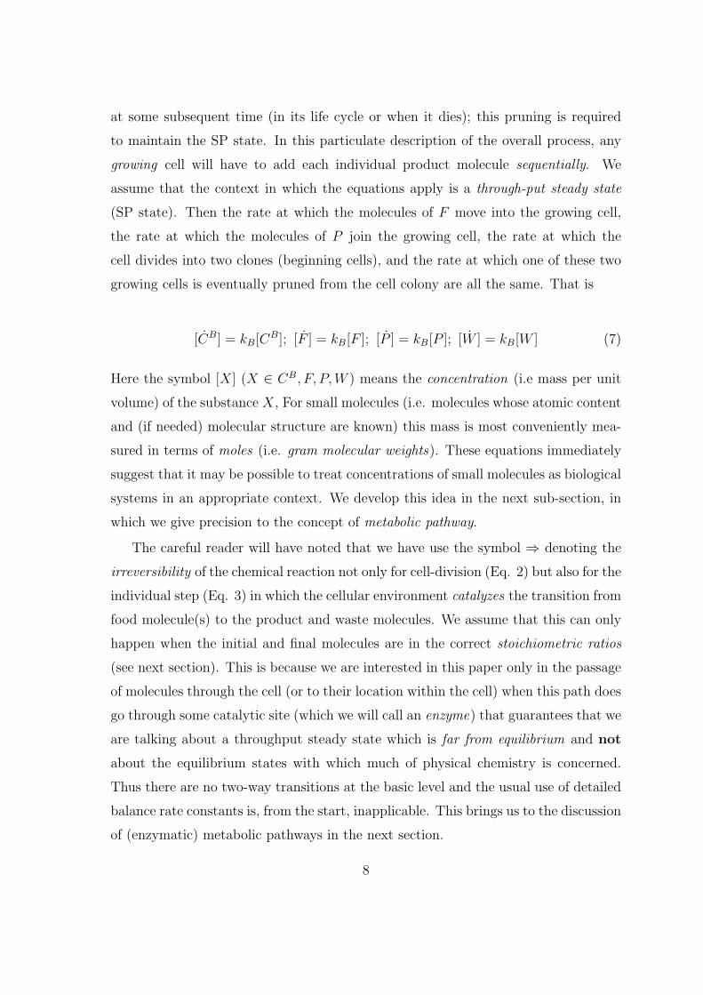
polymer. The second example is illustrated in [7], Fig. 5, p.28, which is reproduced

below, together with its figure caption as Figure 1. I trust that, after the above sketch

of how the whole thing works, this captioned figure is self-explanatory.

What Fig. 1 does not point out is that the genetic control mechanism acts on a

long time scale, appropriate to a secular change in the rate and/or amount at which

food is flowing into the system from the environment, while the internal control loop

acts on a shorter time scale which can smooth out short term fluctuations in the

concentrations due to other causes. That this feedback is stable follows immediately

from the irreversibility of the direction of flow at the two enzymes. These absorbing

state phase transitions (from M + X to (X ·M) and from (X ·M) to X + P — with

the return control loop path that takes X “back” to the initiating phase transition in

place) also enforce the stoichiometric set points for both the interior and the exterior

rate control. The rate controlled range of kB comes from: a) the fact that the number

of ribosomes per cell increases with kB; b) the fact that the range of kB is limited

at the upper end by the maximum number of ribosomes which the cell can hold in

a steady state; c) the fact that the range of kB is limited at the lower end by the

minimum amount of nutrient which will allow, at least, the minimum stable number

of cells to maintain themselves in the chemostat at the flow rates for nutrient input

and for the solvent carrier input.

18

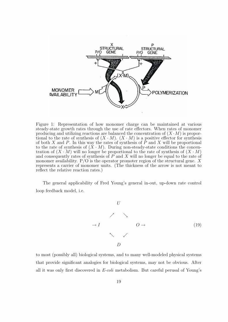
Figure 1: Representation of how monomer charge can be maintained at varioussteady-state growth rates through the use of rate effectors. When rates of monomerproducing and utilizing reactions are balanced the concentration of (X ·M) is propor-tional to the rate of synthesis of (X ·M). (X ·M) is a positive effector for synthesisof both X and P . In this way the rates of synthesis of P and X will be proportionalto the rate of synthesis of (X ·M). During non-steady-state conditions the concen-tration of (X ·M) will no longer be proportional to the rate of synthesis of (X ·M)and consequently rates of synthesis of P and X will no longer be equal to the rate ofmonomer availability. P/O is the operator promoter region of the structural gene. Xrepresents a carrier of monomer units. (The thickness of the arrow is not meant toreflect the relative reaction rates.)

The general applicability of Fred Young’s general in-out, up-down rate control

loop feedback model, i.e.

U

↗ ↘

→ I O → (19)

↖ ↙

D

to most (possibly all) biological systems, and to many well-modeled physical systems

that provide significant analogies for biological systems, may not be obvious. After

all it was only first discovered in E-coli metabolism. But careful perusal of Young’s

19

thesis[7], should begin to remove doubt on that score. The thesis was deliberately

undertaken, not to solve a specific problem but to find a mechanism that could ac-

count in a general way for how rate control of metabolism can lead to multiple rates of

growth in stable populations and for growing systems exhibiting balanced exponential

growth. Subsequent developments in biology and other fields provide ample evidence

for the fact that Young’s model is ubiquitous in its applicability. This topic will be

discussed in[11], where the connected chain: non-equilibrium steady state → absorb-

ing state phase transition → allometric scaling laws → fractal scaling → Kolmogorov

scaling is developed. The abstract of an earlier talk by Young on this subject at an

international meeting in Shanghai is presented here as Appendix 1.

Although the primary purpose of this paper was to prepare a mathematical

and logical basis for the Young model, whose technical structure will be presented

elsewhere[8], we wish to also take this occasion to point out that, once the biolog-

ical principles are understood, the top-down analysis of metabolic pathways which

Young’s general model makes possible did not have to wait for mathematical devel-

opment in order to be applied. The underlying logic and analytic framework have

been used as the basis for research to identify, select and assemble data from the pub-

lished literature. This data can then be used to create models for Cancer Cachexia

and other diseases. This systematic approach, starting from Young’s 1977 thesis[7],

developed by Young and collaborators and now called HiNET, then allows combined

drug therapies appropriate to these diseases to be constructed. The technology has

led to a venture capital backed company with a portfolio of high potential ideas, one

already in FDA-approved Phase 2 trial and two more likely to enter trial in 2008.

The problem of cancer cachexia can be briefly described as follows. Normal nutri-

tion for our species and many others has a replete-hungry cycle with on-off switches

changing the metabolic pathways between the two stable states. In certain shock

states, there a great need for nutrition at any cost and the body in these states starts

eating anything inside it, including its own structure. Normally this state turns

off when the danger is past, but cancer and some cancer therapies can produce a

shock state that does not return to normal; consequently the body wastes away even

though ample nutrition is provided by injection into the veins. Using his analysis,

20

Young found a way to treat the patient with combinations of FDA-approved drugs.

They alter the concentrations of small molecules in the direction which returns the

body to normal nutritional states and solves the problem. Preliminary clinical trials

were successful and second stage trials were approved. An older short report of this

is given in Appendix 2.

In conclusion, I believe that Young’s control loop feedback in-out: up-down cycle

model for a throughput system is a good candidate to become an emergent fundamen-

tal law of biological systems going beyond the Darwinian organizing principle. Using

such control loops as coupled nodes in a hierarchical model for top-down analysis

of functional metabolic pathways, of which the first examples are Young’s HiNET

models, bids fair to become a fruitful research tool for uncovering novel emergent

biological organizing principles during the 21st century.

3 Acknowledgments

This paper rests primarily on the decades of work by Fredric S. Young on his unique

approach to the problem of the organization and integration of biological systems. I

am most indebted to him for his invitation to participate in this research. I am also

indebted to James V. Lindesay for his collaboration on clarifying the mathematical

structure of the feedback system involved in the two-enzyme control loop, and to both

of them for the three-way discussions we had during 2004-2006. I owe much to the

the clarification of the logical and philosophical structure of what we are attempting

to do provided by Walter R. Lamb while he was still with us.

4 Appendix 1: The Universal Modular Organiza-

tion of Hierarchical Control Networks in Biology

Fredric S.Young

Vicus Biosciences

Fredric S.Young, Vicus Biosciences [now Vicus Therapeutics, LLC]

21

Progress in the physical sciences have always involved conceptual and theoretical

simplification and unification. Modern biology has resisted this tendency and has

focused almost completely on the details. The sequencing of the human genome has

not been translated into comprehensive models and has not led to new therapies.

Using reverse engineering, we have abstracted a theoretical description of the uni-

versal modular organization of biological control systems which are modeled as the

construction of a fractal representing the hierarchical control network or HiNet. Dis-

ease therapy becomes a problem of shifting the state of the HiNet to a configuration

closer to normal homeostasis. This has enabled the rational and systematic develop-

met of combination therapies for clinical trials. An emphasis on energy and control

manifolds connects this approach to catastrophe theory. The modularity of HiNet

allows a hierarchical network decomposition and modeling of local processes on low

dimensional control manifolds. Modeling of the integrated global organization of a

biological system requires control spaces of many more dimensions than 3 as stated

by Thom in Structural Stability and Morphogenesis. A HiNet model of allometric

scaling supports the recent application by Ji-Huan He of El Naschie’s ε∞ theory to

biology. (Abstract of paper presented at the 2005 International Symposium on Non-

Linear Dynamics: Celebration of M.S. El-Naschie’s 60 Anniversary, December 20-21,

Shanghai, China)

5 Appendix 2: The Obsolescence of Reductionist

Biology: Systems Biology Modeling and Cancer

Cachexia Therapy Development Based on Emer-

gent Patterns of Organization Rather Than on

Genes and Molecules

Dr. Fredric Young, Chief Scientist, Vicus Therapeutics, LLC

Vicus has developed a hierarchical network (HiNET) model of emergent patterns

of organization based on principles of self-organized criticality, phase-transitions, in-

22

tegral control and reaction blocks. We will describe our HiNET model of cancer

cachexia, a catastrophic wasting disorder secondary to advanced cancer, and its pre-

dicted EKG-based biomarkers and reaction-block drug targets. We will show data

from our retrospective and prospective VT-122 clinical trials and contrast our clinical

results with previous failed attempts targeting specific dysregulated pathways and

proteins. (Abstract of paper presented at Beyond the Genome 2006: Top Ten Oppor-

tunities in the Post-Genome Era, June 19=21, 2006, Fairmont Hotel, San Francisco,

California.)

References

[1] P.W.Anderson, “More is Different”, Science 177, 393-396 (1972).

[2] R.B.Laughlin and David Pines, “The Theory of Everything”, PNAS 97, 28-31

(2000).

[3] R.B.Laughlin A Diffrent Universe: Reinventing Physics from the Bottom Down,

Basic Books, New York (2005).

[4] A.Leggett, Physics Today, October 2005, pp. 77-78.

[5] F.S.Young: Proc ANPA 12, “Pattern, Form,Chaos”, pp. 74-83 + 24 colored

figures; — 13, “Fractal Geometry and Quantum Mechanics”, pp. 124-138; — 14,

“Chaos, Biology and Physics”, pp. 131-143.

[6] F.S.Young, private communications to HPN.

[7] F.S.Young, “Biological Growth Rate and the Metabolic Regulation of Gene Ex-

pression”, PhD Thesis, University of Michigan (1977).

[8] F.S.Young, J.V.Lindesay, H.P.Noyes and W.R.Lamb, “A Paradigm for Biologi-

cal Systems based on Enzymatic Rate control” (in preparation); here the word

paradigm is deliberately used with the connotations introduced by Kuhn[12].

23

[9] O.Mallφe and N.O.Kjeldgaard, Control of macro-molecular synthesis,

W.A.Benjamin Inc., Amsterdam, New York (1966).

[10] G.Grinstein, Z.W.Lai and D.A.Browne, Physical Review A 40, 4820 (1989).

[11] F.S.Young, A Paradigm for Biology’s Next Revolution (in preparation).

[12] T.S.Kuhn, The Structure of Scientific Revolutions, Univ. of Chicago Press, 1962.

24