On autoencoder scoring

Hanna Kamyshanska kamyshanska@fias.uni-frankfurt.de

Goethe Universitat Frankfurt, Robert-Mayer-Str. 11-15, 60325 Frankfurt, Germany

Roland Memisevic memisevr@iro.umontreal.ca

University of Montreal, CP 6128, succ Centre-Ville, Montreal H3C 3J7, Canada

Abstract

Autoencoders are popular feature learningmodels because they are conceptually sim-ple, easy to train and allow for efficient in-ference and training. Recent work has shownhow certain autoencoders can assign an un-normalized “score” to data which measureshow well the autoencoder can represent thedata. Scores are commonly computed by us-ing training criteria that relate the autoen-coder to a probabilistic model, such as theRestricted Boltzmann Machine. In this pa-per we show how an autoencoder can assignmeaningful scores to data independently oftraining procedure and without reference toany probabilistic model, by interpreting it asa dynamical system. We discuss how, and un-der which conditions, running the dynamicalsystem can be viewed as performing gradientdescent in an energy function, which in turnallows us to derive a score via integration.We also show how one can combine multiple,unnormalized scores into a generative classi-fier.

1. Introduction

Unsupervised learning has been based traditionally onprobabilistic modeling and maximum likelihood esti-mation. In recent years, a variety of models have beenproposed which define learning as the construction ofan unnormalized energy surface and inference as find-ing local minima of that surface. Training such energy-based models amounts to decreasing energy near theobserved training data points and increasing it every-where else (Hinton, 2002; lec). Maximum likelihood

Proceedings of the 30 th International Conference on Ma-chine Learning, Atlanta, Georgia, USA, 2013. JMLR:W&CP volume 28. Copyright 2013 by the author(s).

learning can be viewed as a special case, where theexponential of the negative energy integrates to 1.

The probably most successful recent examples of non-probabilistic unsupervised learning are autoencodernetworks, which were shown to yield state-of-the-artperformance in a wide variety of tasks, ranging fromobject recognition and learning invariant representa-tions to syntatic modeling of text (Le et al., 2012;Socher et al., 2011; Rolfe & LeCun, 2013; Swerskyet al., 2011; Vincent, 2011; Memisevic, 2011; Zou et al.,2012). Learning amounts to minimizing reconstructionerror using back-prop. Typically, one regularizes theautoencoder, for example, by adding noise to the in-put data or by adding a penalty term to the trainingobjective (Vincent et al., 2008; Rifai et al., 2011).

The most common operation after training is to in-fer the latent representation from data, which can beused, for example, for classification. For the autoen-coder, extracting the latent representation amountsto evaluating a feed-forward mapping. Since trainingis entirely unsupervised, one autoencoder is typicallytrained for all classes, and it is the job of the classifierto find and utilize class-specific differences in the repre-sentation. This is in contrast to the way in which prob-abilistic models have been used predominantly in thepast: Although probabilistic models (such as Gaussianmixtures) may be used to extract class-independentfeatures for classification, it has been more commonto train one model per class and to subsequently useBayes’ rule for classification (Duda & Hart, 2001). Inthe case where an energy-based model can assign con-fidence scores to data, such class-specific unsupervisedlearning is possible without Bayes’ rule: When scoresdo not integrate to 1 one can, for example, train aclassifier on the vector of scores across classes (Hin-ton, 2002), or back-propagate label information to theclass-specific models using a “gated softmax” response(Memisevic et al., 2011).

On autoencoder scoring

1.1. Autoencoder scoring

It is not immediatly obvious how one may computescores from an autoencoder, because the energy land-scape does not come in an explicit form. This is incontrast to undirected probability models like the Re-stricted Boltzmann Machine (RBM) or Markov Ran-dom Fields, which define the score (or negative energy)as an unnormalized probability distribution. Recentwork has shown that autoencoders can assign scores,too, if they are trained in a certain way: If noise isadded to the input data during training, minimizingsquared error is related to performing score matching(Hyvarinen, 2005) in an undirect probabilistic model,as shown by (Swersky et al., 2011) and (Vincent, 2011).This, in turn, makes it possible to use the RBM energyas a score. A similar argument can be made for other,related training criteria. For example, (Rifai et al.,2011) suggest training autoencoders using a “contrac-tion penalty” that encourages latent representations tobe locally flat, and (Alain & Bengio, 2013) show thatsuch regularization penalty allows us to interpret theautoencoder reconstruction function as an estimate ofthe gradient of the data log probability.1

All these approaches to defining confidence scores relyon a regularized training criterion (such as denoisingor contraction), and scores are computed by using therelationship with a probabilistic model. As a resultscores can be computed easily only for autoencodersthat have sigmoid hidden unit activations and linearoutputs, and that are trained by minimizing squarederror (Alain & Bengio, 2013). The restriction of ac-tivation function is at odds with the growing interestin unconventional activation functions, like quadraticor rectified linear units which seem to work better insupervised recognition tasks (eg., (Krizhevsky et al.,2012)).

In this work, we show how autoencoder confidencescores may be derived by interpreting the autoencoderas a dynamical system. The view of the autoencoderas a dynamical system was proposed by (Seung, 1998),who also demonstrated how de-noising as a learningcriterion follows naturally from this perspective. Tocompute scores, we will assume “tied weights”, thatis, decoder and encoder weights are transposes of eachother. In contrast to probabilistic arguments basedon score matching and regularization (Swersky et al.,2011; Vincent, 2011; Alain & Bengio, 2013), the dy-namical systems perspective allows us to assign con-

1The term “score” is also frequently used to refer to thegradient of the data log probability. In this paper we usethe term to denote a confidence value that the autoencoderassigns to data.

fidence scores to networks with sigmoid output units(binary data) and arbitrary hidden unit activations (aslong as these are integrable). In contrast to (Rolfe &LeCun, 2013), we do not address the role of dynamicsin learning. In fact, we show how one may derive con-fidence scores that are entirely agnostic to the learningprocedure used to train the model.

As an application of autoencoder confidence scores wedescribe a generative classifier based on class-specificautoencoders. The model achieves 1.27% error rate onpermutation invariant MNIST, and yields competitiveperformance on the deep learning benchmark datasetby (Larochelle et al., 2007).

2. Autoencoder confidence scores

Autoencoders are feed forward neural networks usedto learn representations of data. They map input datato a hidden representation using an encoder function

h(Wx+ bh

)(1)

from which the data is reconstructed using a lineardecoder

r(x) = Ah(Wx+ bh

)+ br (2)

We shall assume that A = WT in the following (“tiedweights”). This is common in practice, because it re-duces the number of parameters and because relatedprobabilistic models, like the RBM, are based on tiedweights, too.

For training, one typically minimizes squared recon-struction error (r(x)− x)2 for a set of training cases.When the number of hidden units is small, autoen-coders learn to perform dimensionality reduction. Inpractice, it is more common to learn sparse represen-tations by using a large number of hidden units andtraining with a regularizer (eg., (Rifai et al., 2011; Vin-cent et al., 2008)). A wide variety of models can belearned that way, depending on the activation func-tion, number of hidden units and nature of the regu-larization during training. The function h(·) can bethe identity or it can be an element-wise non-linearity,such as a sigmoid function. Autoencoders defined us-ing Eq. 2 with tied weights and logistic sigmoid non-

linearity h(a) =(1 + exp(−a)

)−1are closely related

to RBMs (Swersky et al., 2011; Vincent, 2011; Alain& Bengio, 2013), one can assign confidence scores todata in the form of unnormalized probabilities.

For binary data, the decoder typically gets replaced by

r(x) = σ(Ah(Wx+ bh

)+ br

)(3)

and training is done by minimizing cross-entropy loss.Even though confidence scores (negative free energies)

On autoencoder scoring

are well-defined for binary output RBMs, there hasbeen no analogous score function for the autoencoder,because the relationships with score matching breaksdown in the binary case (Alain & Bengio, 2013). Aswe shall show, the perspective of dynamical systemsallows us to attribute the missing link to the lack ofsymmetry. We also show how we can regain symme-try and thereby obtain a confidence score for binaryoutput autoencoders by applying a log-odds transfor-mation on the outputs of the autoencoder.

2.1. Reconstruction as energy minimization

Autoencoders may be viewed as dynamical systems,by noting that the function r(x)−x (using the defini-tion in Eq. 2) is a vector field which represents the lin-ear transformation that x undergoes as a result of ap-plying the reconstruction function r(x) (Seung, 1998;Alain & Bengio, 2013). Repeatedly applying the re-construction function (possibly with a small inferencerate ε) to an initial x will trace out a non-linear tra-jectory x(t) in the data-space.

If the number of hidden units is smaller than the num-ber of data dimensions, then the set of fixed pointsof the dynamical system will be approximately a low-dimensional manifold in the data-space (Seung, 1998).For overcomplete hiddens it can be a more complexstructure.

(Alain & Bengio, 2013), for example, show that fordenoising and contractive autoencoder, the reconstruc-tion is proportional to the derivative of the log proba-bility of x:

r(x)− x = λ∂ logP (x)

∂(x)+O(λ) (4)

Running the autoencoder by following a trajectory asprescribed by the vector field may also be viewed inanalogy to running a Gibbs sampler in an RBM, wherethe fixed points play the role of a maximum probability“ridge” and where the samples are deterministic notstochastic.

Some vector fields can be written as the derivative of ascalar field: In such a case, running the dynamical sys-tem can be thought of as performing gradient descentin the scalar field. We may call this scalar field energyE(x) and interpret the vector field as a correspond-ing “force” in analogy to physics, where the potentialforce acting on a point is the gradient of the potentialenergy at that point. The autoencoder reconstructionmay thus be viewed as pushing data samples in thedirection of lower energy (Alain & Bengio, 2013).

The reason why evaluating the potential energy for

the autoencoder would be useful is that it allows us toasses how much the autoencoder “likes” a given inputx (up to a normalizing constant which is the samefor any two inputs). That way, the potential energyplays an analogous role to the free energy in an RBM(Hinton, 2002; Swersky et al., 2011). As shown by(Alain & Bengio, 2013), the view of the autoencoder asmodeling an energy surface implies that reconstructionerror is not a good measure of confidence, because thereconstruction error will be low at both local minimaand local maxima of the energy.

A simple condition for a vector field to be a gradientfield is given by Poincare‘s integrability criterion: Forsome open, simple connected set U , a continuouslydifferentiable function F : U → Rn defines a gradientfield if and only if

∂Fj(x)

∂xi=∂Fi(x)

∂xj, ∀i, j = 1..n (5)

In other words, integrability follows from symmetry ofthe partial derivatives.

Consider an autoencoder with shared weight matrixW and biases bh and br, which has some activationfunction h(.) (e.g. sigmoid, hyperbolic tangent, lin-ear). We have:

∂(rm(x)− xm)

∂xn=

∑j

Wmj∂h(Wx+ bh)

∂(Wx+ bh)Wnj − 1

=∂(rn(x)− xn)

∂xm(6)

so the integrability criterion is satisfied.

2.2. Computing the energy surface

One way to find the potential energy whose derivativeis r(x)−x, is to integrate the vector field (compute itsantiderivative).2 This turns out to be fairly straight-forward for autoencoders with a single hidden layer,linear output activations, and symmetric weights, inother words

r(x) = WTh(Wx+ bh

)+ br (7)

2After computing the energy function, it is easy tocheck, in hindsight, whether the vector field defined bythe autoencoder is really the gradient field of that energyfunction: Compute the derivative of the energy, and checkif it is equal to r(x) − x. For example, to check the cor-rectness of Eqs. 11 and 13 differentiate the equations wrt.x.

On autoencoder scoring

Figure 1. Some hidden unit activation functions and their integrals.

where h(·) is an elementwise activation function, suchas the sigmoid. We can now write

F (x) =

∫(r(x)− x) dx

=

∫ (WTh

(Wx+ bh

)+ br − x

)dx

= WT

∫h(Wx+ bh

)dx+

∫(br − x) dx

(8)

By defining the auxiliary variables u = Wx+ bh andusing

du

dx= WT ⇔ dx = W−Tdu (9)

we get

F (x) = WTW−T

∫h(u) du+ br

Tx− 1

2x2 + const

=

∫h(u) du+ br

Tx− 1

2x2 + const

=

∫h(u) du− 1

2

(x− br

)2+

1

2br

Tbr + const

=

∫h(u) du− 1

2

(x− br

)2+ const (10)

where the last equation uses the fact that br does notdepend on x.

If h(u) is an elementwise activation function, then thefinal integral is simply the sum over the antiderivativesof the hidden unit activation functions applied to x.In other words, we can compute the integral using thefollowing recipe:

1. compute the net inputs to the hidden units:

Wx+ bh

2. compute hidden unit activations using the an-tiderivative of h(u) as the activation function

3. sum up the activations and subtract 12

(x− br

)2Example: sigmoid hiddens. In the case of sigmoidactivation functions h(u) = (1 + exp(−u))−1, we get

Fsigmoid(x)

=

∫(1 + exp(−u))−1 du− 1

2

(x− br

)2+ const

=∑k

log(1 + exp(WT·kx+ bhk))− 1

2

(x− br

)2+ const

(11)

which is identical to the free energy in a binary-Gaussian RBM (eg., (Welling et al., 2005)). It is inter-esting to note that in the case of contractive or denois-ing training (Alain & Bengio, 2013), the energy can infact be shown to approximate the log-probability ofthe data (cf., Eq. 4):

F (x) :=

∫(r(x)− x) dx ∝ logP (x) (12)

But Eq. 11 is more general as it holds independentlyof the training procedure.

Example: linear hiddens. The antiderivative of thelinear activation, h(u) = u, is u2, so for PCA and alinear autoencoder, it is simply the norm of the latentrepresentation. More precisely, we have

Flinear(x) =

∫u du− 1

2

(x− br

)2+ const

=1

2uTu− 1

2

(x− br

)2+ const

=1

2(Wx+ bh)T(Wx+ bh)− 1

2

(x− br

)2+ const

(13)

It is interesting to note that, if we disregard biases andassumeWWT = I (the PCA solution), then Flinear(x)turns into the negative squared reconstruction error.

On autoencoder scoring

This is how one would typically assign confidences toPCA models, for example, in a PCA based classfier.

It is straightforward to calculate the energies for otherhidden unit activations, including those for which theenergy cannot be normalized, in which case there is nocorresponding RBM. Two commonly deployed activa-tion functions are, for example: the rectifier, whose

antiderivative is the “half-square” (sign(x)+1)2 x2, and

the softplus activation whose antiderivative is the so-called polylogarithm. A variety of activation functionsand their antiderivatives are shown in Fig. 1.

2.3. Binary data

When dealing with binary data it is common to usesigmoid activations on the outputs:

r(x) = σ(WTh

(Wx+ bh

)+ br

)(14)

and training the model using cross-entropy (but like inthe case of real outputs, the criterion used for trainingwill not be relevant to compute scores). In the case ofsigmoid outputs activations, the integrability criterion(Eq. 6) does not hold, because of the lack of symmetryof the derivatives. However, we can obtain confidencescores by monotonically transforming the vector spaceas follows: We apply the inverse of the logistic sigmoid(the “log-odds” transformation)

ξ(x) = log( x

1− x)

(15)

in the input domain. Now we can define the new vectorfield

v(x) = ξ(r(x))− ξ(x)

= ξ(σ(WTh

(Wx+ bh

)+ br

))− log

( x

1− x)

= WTh(Wx+ bh

)+ br − log

( x

1− x)

(16)

The vector field v(x) has the same fixed points asr(x)− x, because invertibility of ξ(x) implies

r(x) = x ⇔ ξ(r(x)) = ξ(x) (17)

So the original and transformed autoencoder convergeto the same representations of x. By integrating v(x),we get

F (x) =

∫h(u) du+ br

Tx

− log(1− x

)− x log

( x

1− x)

+ const

(18)

Due to the convention 0 · log 0 = 0, the second term,

− log(1 − x

)− x log

(x

1−x

), vanishes for binary data

(Cover & Thomas, 1991). In that case, the energytakes exactly the same form as the free energy of abinary output RBM with binary hidden units (Hin-ton, 2002). However, hidden unit activation functionscan be chosen arbitrarily and enter the score using therecipe described above. Also, training data may notalways be binary. When it takes on values between 0and 1, the log-terms do not equal 0 and have to beincluded in the energy computation.

3. Combining autoencoders forclassification

Being able to assign unnormalized scores to data canbe useful in a variety of tasks, including visualizationor classification based on ranking of data examples.Like for the RBM, the lack of normalization causesscores to be relative not absolute. This means that wecan compare the scores that an autoencoder assignsto multiple data-points but we cannot compare thescores that multiple autoencoders assign to the samedata-point. We shall now discuss how we can turnthese into a classification decision.

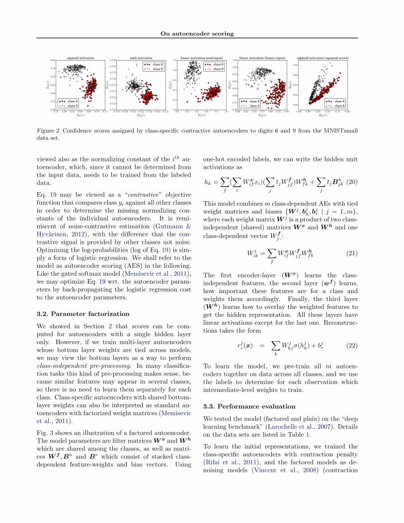
Fig. 2 shows exemplary energies that various typesof contractive autoencoder (cAE, (Rifai et al., 2011)),trained on MNISTsmall digits 6 and 9, assign to testcases from those classes. It shows that all models yieldfairly well separated confidence scores, when the apro-priate anti-derivatives are used. Squared error on thesigmoid networks separates these examples fairly welltoo (rightmost plot). However, in a multi-class task,using reconstruction error typically does not work well(Susskind et al., 2011), and it is not a good confi-dence measure as we discussed in Section 2. As weshall show, one can achieve competitive classificationperformance on MNIST and other data-sets by usingproperly “calibrated” energies, however.

3.1. Supervised finetuning

Since the energy scores are unnormalized, we cannotuse Bayes’ rule for classification unlike with directedgraphical models. Here, we adopt the approach pro-posed by (Memisevic et al., 2011) for Restricted Boltz-mann Machines and adopt it to autoencoders.

In particular, denoting the energy scores that theautoencoders for different classes assign to data asEi(x), i = 1, . . . ,K, we can define the conditional dis-tribution over classes yi as the softmax response

P (yi|x) =exp(Ei(x) + Ci)∑j exp(Ej(x) + Cj)

(19)

where Ci is the bias term for class yi. Each Ci may be

On autoencoder scoring

0.45 0.50 0.55 0.60 0.65 0.70 0.75

E6(x)

0.50

0.55

0.60

0.65

0.70

0.75

0.80

E9(x

)

sigmoid activation

class 6class 9

0.719 0.720 0.721 0.722 0.723 0.724 0.725

E6(x)

0.711

0.712

0.713

0.714

0.715

0.716

0.717

0.718

0.719

E9(x

)

tanh activation

class 6class 9

0.0 0.2 0.4 0.6 0.8 1.0

E6(x)

0.0

0.2

0.4

0.6

0.8

1.0

E9(x

)

linear activation (real input)

class 6class 9

0.60 0.65 0.70 0.75 0.80 0.85 0.90

E6(x)

0.70

0.75

0.80

0.85

0.90

0.95

1.00

1.05

E9(x

)

linear activation (binary input)

class 6class 9

−0.05 0.00 0.05 0.10 0.15 0.20

R6(x)

0.00

0.02

0.04

0.06

0.08

R9(x

)

sigmoid activation (squared errors)

class 6class 9

Figure 2. Confidence scores assigned by class-specific contractive autoencoders to digits 6 and 9 from the MNISTsmalldata set.

viewed also as the normalizing constant of the ith au-toencoder, which, since it cannot be determined fromthe input data, needs to be trained from the labeleddata.

Eq. 19 may be viewed as a “contrastive” objectivefunction that compares class yi against all other classesin order to determine the missing normalizing con-stants of the individual autoencoders. It is remi-niscent of noise-contrastive estimation (Gutmann &Hyvarinen, 2012), with the difference that the con-trastive signal is provided by other classes not noise.Optimizing the log-probabilities (log of Eq. 19) is sim-ply a form of logistic regression. We shall refer to themodel as autoencoder scoring (AES) in the following.Like the gated softmax model (Memisevic et al., 2011),we may optimize Eq. 19 wrt. the autoencoder param-eters by back-propagating the logistic regression costto the autoencoder parameters.

3.2. Parameter factorization

We showed in Section 2 that scores can be com-puted for autoencoders with a single hidden layeronly. However, if we train multi-layer autoencoderswhose bottom layer weights are tied across models,we may view the bottom layers as a way to performclass-independent pre-processing. In many classifica-tion tasks this kind of pre-processing makes sense, be-cause similar features may appear in several classes,so there is no need to learn them separately for eachclass. Class-specific autoencoders with shared bottom-layer weights can also be interpreted as standard au-toencoders with factorized weight matrices (Memisevicet al., 2011).

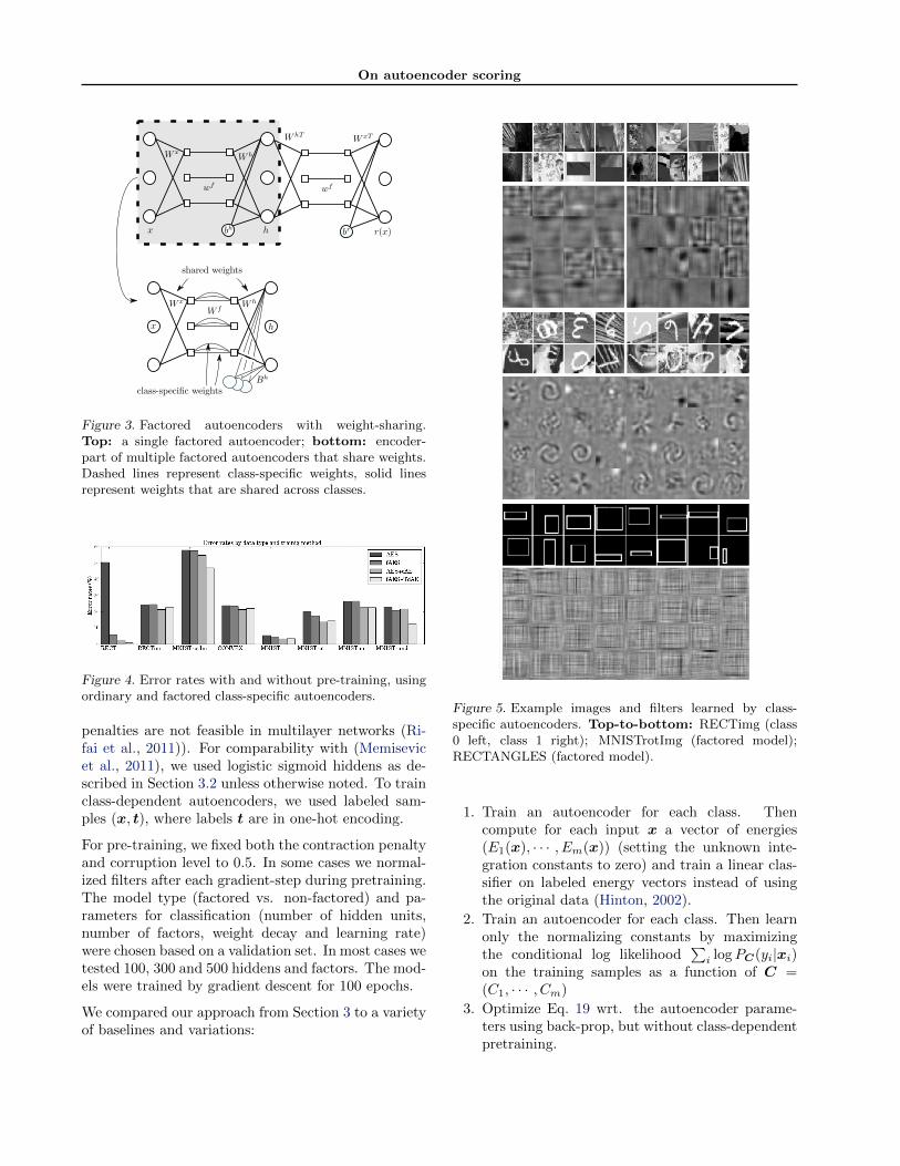
Fig. 3 shows an illustration of a factored autoencoder.The model parameters are filter matricesW x andW h

which are shared among the classes, as well as matri-ces W f ,Bh and Br which consist of stacked class-dependent feature-weights and bias vectors. Using

one-hot encoded labels, we can write the hidden unitactivations as

hk =∑f

(∑i

Wxifxi)(

∑j

tjWfjf )Wh

fk +∑j

tjBhjk (20)

This model combines m class-dependent AEs with tiedweight matrices and biases {W j , bjh, b

jr | j = 1..m},

where each weight matrixW j is a product of two class-independent (shared) matrices W x and W h and one

class-dependent vector W fj .:

W jik =

∑f

WxifW

fjfW

hfk (21)

The first encoder-layer (W x) learns the class-independent features, the second layer (wf ) learns,how important these features are for a class andweights them accordingly. Finally, the third layer(W h) learns how to overlay the weighted features toget the hidden representation. All these layers havelinear activations except for the last one. Reconstruc-tions takes the form

rji (x) =∑k

W jkjσ(hjk) + bjr (22)

To learn the model, we pre-train all m autoen-coders together on data across all classes, and we usethe labels to determine for each observation whichintermediate-level weights to train.

3.3. Performance evaluation

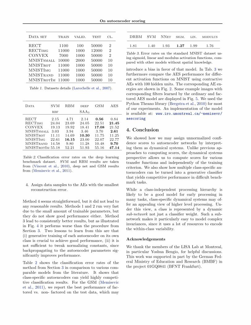
We tested the model (factored and plain) on the “deeplearning benchmark” (Larochelle et al., 2007). Detailson the data sets are listed in Table 1.

To learn the initial representations, we trained theclass-specific autoencoders with contraction penalty(Rifai et al., 2011), and the factored models as de-noising models (Vincent et al., 2008) (contraction

On autoencoder scoring

Figure 3. Factored autoencoders with weight-sharing.Top: a single factored autoencoder; bottom: encoder-part of multiple factored autoencoders that share weights.Dashed lines represent class-specific weights, solid linesrepresent weights that are shared across classes.

Figure 4. Error rates with and without pre-training, usingordinary and factored class-specific autoencoders.

penalties are not feasible in multilayer networks (Ri-fai et al., 2011)). For comparability with (Memisevicet al., 2011), we used logistic sigmoid hiddens as de-scribed in Section 3.2 unless otherwise noted. To trainclass-dependent autoencoders, we used labeled sam-ples (x, t), where labels t are in one-hot encoding.

For pre-training, we fixed both the contraction penaltyand corruption level to 0.5. In some cases we normal-ized filters after each gradient-step during pretraining.The model type (factored vs. non-factored) and pa-rameters for classification (number of hidden units,number of factors, weight decay and learning rate)were chosen based on a validation set. In most cases wetested 100, 300 and 500 hiddens and factors. The mod-els were trained by gradient descent for 100 epochs.

We compared our approach from Section 3 to a varietyof baselines and variations:

Figure 5. Example images and filters learned by class-specific autoencoders. Top-to-bottom: RECTimg (class0 left, class 1 right); MNISTrotImg (factored model);RECTANGLES (factored model).

1. Train an autoencoder for each class. Thencompute for each input x a vector of energies(E1(x), · · · , Em(x)) (setting the unknown inte-gration constants to zero) and train a linear clas-sifier on labeled energy vectors instead of usingthe original data (Hinton, 2002).

2. Train an autoencoder for each class. Then learnonly the normalizing constants by maximizingthe conditional log likelihood

∑i logPC(yi|xi)

on the training samples as a function of C =(C1, · · · , Cm)

3. Optimize Eq. 19 wrt. the autoencoder parame-ters using back-prop, but without class-dependentpretraining.

On autoencoder scoring

Data set train valid. test cl.

RECT 1100 100 50000 2RECTimg 11000 1000 12000 2CONVEX 7000 1000 50000 2MNISTsmall 10000 2000 50000 10MNISTrot 11000 1000 50000 10MNISTImg 11000 1000 50000 10MNISTrand 11000 1000 50000 10MNISTrotIm 11000 1000 50000 10

Table 1. Datasets details (Larochelle et al., 2007).

Data SVM RBM deep GSM AES

rbf SAA3

RECT 2.15 4.71 2.14 0.56 0.84RECTimg 24.04 23.69 24.05 22.51 21.45CONVEX 19.13 19.92 18.41 17.08 21.52MNISTsmall 3.03 3.94 3.46 3.70 2.61MNISTrot 11.11 14.69 10.30 11.75 11.25MNISTImg 22.61 16.15 23.00 22.07 22.77MNISTrand 14.58 9.80 11.28 10.48 9.70MNISTrotIm 55.18 52.21 51.93 55.16 47.14

Table 2. Classification error rates on the deep learningbenchmark dataset. SVM and RBM results are takenfrom (Vincent et al., 2010), deep net and GSM resultsfrom (Memisevic et al., 2011).

4. Assign data samples to the AEs with the smallestreconstruction error.

Method 4 seems straightforward, but it did not lead toany reasonable results. Methods 1 and 2 run very fastdue to the small amount of trainable parameters, butthey do not show good performance either. Method3 lead to consistently better results, but as illustratedin Fig. 4 it performs worse than the procedure fromSection 3. Two lessons to learn from this are that(i) generative training of each autoencoder on its ownclass is crucial to achieve good performance, (ii) it isnot sufficient to tweak normalizing constants, sincebackpropagating to the autoencoder parameters sig-nificantly improves performance.

Table 2 shows the classification error rates of themethod from Section 3 in comparison to various com-parable models from the literature. It shows thatclass-specific autoencoders can yield highly competi-tive classification results. For the GSM (Memisevicet al., 2011), we report the best performance of fac-tored vs. non- factored on the test data, which may

DRBM SVM NNet sigm. lin. modulus

1.81 1.40 1.93 1.27 1.99 1.76

Table 3. Error rates on the standard MNIST dataset us-ing sigmoid, linear and modulus activation functions, com-pared with other models without spatial knowledge.

introduce a bias in favor of that model. In Tab. 3 wefurthermore compare the AES performance for differ-ent activation functions on MNIST using contractiveAEs with 100 hidden units. The corresponding AE en-ergies are shown in Fig. 2. Some example images withcorresponding filters learned by the ordinary and fac-tored AES model are displayed in Fig. 5. We used thePython Theano library (Bergstra et al., 2010) for mostof our experiments. An implementation of the modelis available at: www.iro.umontreal.ca/~memisevr/

aescoring

4. Conclusion

We showed how we may assign unnormalized confi-dence scores to autoencoder networks by interpret-ing them as dynamical systems. Unlike previous ap-proaches to computing scores, the dynamical systemsperspective allows us to compute scores for varioustransfer functions and independently of the trainingcriterion. We also show how multiple class-specific au-toencoders can be turned into a generative classifierthat yields competitive performance in difficult bench-mark tasks.

While a class-independent processing hierarchy islikely to be a good model for early processing inmany tasks, class-specific dynamical systems may of-fer an appealing view of higher level processing. Un-der this view, a class is represented by a dynamicsub-network not just a classifier weight. Such a sub-network makes it particularly easy to model complexinvariances, since it uses a lot of resources to encodethe within-class variability.

Acknowledgements

We thank the members of the LISA Lab at Montreal,in particular Yoshua Bengio, for helpful discussions.This work was supported in part by the German Fed-eral Ministry of Education and Research (BMBF) inthe project 01GQ0841 (BFNT Frankfurt).

On autoencoder scoring

References

Alain, G. and Bengio, Y. What regularized auto-encoders learn from the data generating distribu-tion. In International Conference on Learning Rep-resentations (ICLR), 2013.

Bergstra, J., Breuleux, O., Bastien, F., Lamblin, P.,Pascanu, R., Desjardins, G., Turian, J., Warde-Farley, D., and Bengio., Y. Theano: a CPU andGPU math expression compiler. In Python for Sci-entic Computing Conference (SciPy), 2010.

Cover, TM and Thomas, J. Elements of InformationTheory. New York: John Wiley & Sons, Inc, 1991.

Duda, H. and Hart, P. Pattern Classification. JohnWiley & Sons, 2001.

Gutmann, M. U. and Hyvarinen, A. Noise-contrastiveestimation of unnormalized statistical models, withapplications to natural image statistics. Journalof Machine Learning Research, 13:307–361, March2012.

Hinton, G. E. Training products of experts by mini-mizing contrastive divergence. Neural Computation,14(8):1771–1800, 2002.

Hyvarinen, A. Estimation of non-normalized statisti-cal models by score matching. Journal of MachineLearning Research, 6:695–709, December 2005.

Krizhevsky, A., Sutskever, I., and Hinton, G. Ima-genet classification with deep convolutional neuralnetworks. In Advances in Neural Information Pro-cessing Systems (NIPS). 2012.

Larochelle, H., Erhan, D., Courville, A., Bergstra,J., and Bengio, Y. An empirical evaluation ofdeep architectures on problems with many factors ofvariation. In International Conference on MachineLearning (ICML), 2007.

Le, Q., Ranzato, M.A., Monga, R., Devin, M., Chen,K., Corrado, G., Dean, J., and Ng, A. Building high-level features using large scale unsupervised learn-ing. In International Conference on Machine Learn-ing (ICML), 2012.

Memisevic, R. Gradient-based learning of higher-orderimage features. In the International Conference onComputer Vision (ICCV), 2011.

Memisevic, R., Zach, C., Hinton, G., and Pollefeys,M. Gated softmax classification. Advances in NeuralInformation Processing Systems (NIPS), 23, 2011.

Rifai, S., Vincent, P., Muller, X., Glorot, X., andBengio, Y. Contractive auto-encoders: Explicit in-variance during feature extraction. In InternationalConference on Machine Learning (ICML), 2011.

Rolfe, J. T. and LeCun, Y. Discriminative recurrentsparse auto-encoders. In International Conferenceon Learning Representations (ICLR), 2013.

Seung, H.S. Learning continuous attractors in recur-rent networks. Advances in neural information pro-cessing systems (NIPS), 10:654–660, 1998.

Socher, R., Pennington, J., Huang, E. H., Ng, A. Y.,and Manning, C. D. Semi-Supervised Recursive Au-toencoders for Predicting Sentiment Distributions.In Conference on Empirical Methods in NaturalLanguage Processing (EMNLP), 2011.

Susskind, J., Memisevic, R., Hinton, G., and Pollefeys,M. Modeling the joint density of two images under avariety of transformations. In International Confer-ence on Computer Vision and Pattern Recognition(CVPR), 2011.

Swersky, K., Buchman, D., Marlin, B.M., and de Fre-itas, N. On autoencoders and score matching forenergy based models. In International Conferenceon Machine Learning (ICML), 2011.

Vincent, P., Larochelle, H., Bengio, Y., and Manzagol,P. A. Extracting and composing robust featureswith denoising autoencoders. In International Con-ference on Machine Learning (ICML), 2008.

Vincent, P., Larochelle, H., Lajoie, I., Bengio, Y., andManzagol, P.A. Stacked denoising autoencoders:Learning useful representations in a deep networkwith a local denoising criterion. Journal of MachineLearning Research, 11:3371–3408, 2010.

Vincent, Pascal. A connection between score matchingand denoising autoencoders. Neural Computation,23(7):1661–1674, July 2011.

Welling, M., Rosen-Zvi, M., and Hinton, G. Expo-nential family harmoniums with an application toinformation retrieval. Advances in neural informa-tion processing systems (NIPS), 17, 2005.

Zou, W.Y., Zhu, S., Ng, A., and Yu, K. Deep learningof invariant features via simulated fixations in video.In Advances in Neural Information Processing Sys-tems (NIPS), 2012.