
Edwin C. May et al- Decision Augmentation Theory: Toward a Model of Anomalous Mental Phenomena

On Anomalous Ocean Heat Transport toward the Arctic and Associated1
Climate Predictability2
Marius Arthun∗ and Tor Eldevik3
Geophysical Institute, University of Bergen, and Bjerknes Centre for Climate Research, Bergen,
Norway.
J. Climate, In press
4
5
6
7
8
∗Corresponding author address: Marius Arthun, Geophysical Institute, University of Bergen,
Allegaten 70, 5007 Bergen, Norway.
9
10
E-mail: [email protected]
Generated using v4.3.2 of the AMS LATEX template 1

ABSTRACT
A potential for climate predictability is rooted in anomalous ocean heat
transport and its consequent influence on the atmosphere above. Here we
assess the propagation, drivers, and atmospheric impact of heat anomalies
within the northernmost limb of the Atlantic meridional overturning cir-
culation using a multi-century climate model simulation. Consistent with
observation-based inferences, simulated heat anomalies propagate from the
eastern subpolar North Atlantic, into, and through the Nordic Seas. The dom-
inant time scale of associated climate variability in the northern seas is 14
years, including that of observed sea surface temperature and modeled ocean
heat content, air–sea heat flux, and surface air temperature. A heat budget
analysis reveals that simulated ocean heat content anomalies are driven by
poleward ocean heat transport, primarily related to variable volume transport.
The ocean’s influence on the atmosphere, and hence regional climate, is mani-
fested in the model by anomalous ocean heat convergence driving subsequent
changes in surface heat fluxes and surface air temperature. The documented
northward propagation of thermohaline anomalies in the northern seas and
their consequent imprint on the regional atmosphere – including the existence
of a common decadal time scale of variability – detail a key aspect of eventual
climate predictability.
12
13
14
15
16
17
18
19
20
21
22
23
24
25
26
27
28
29
30
2

1. Introduction31
The Atlantic region exhibits distinct interannual to multidecadal variability (Deser and Black-32
mon 1993; Kushnir 1994; Frankcombe et al. 2010; Williams et al. 2014), reflected in upper-ocean33
thermohaline anomalies that propagate persistently through the North Atlantic Ocean and Nordic34
Seas toward the Arctic (Sutton and Allen 1997; Polyakov et al. 2005; Holliday et al. 2008).35
Decadal variability in ocean temperature plays an important role in the marine climate system (e.g.,36
Drinkwater et al. 2014), influencing marine life from primary production to cod stocks (Helland-37
Hansen and Nansen 1909; Hatun et al. 2009). Ocean heat anomalies also play an important role38
in Arctic sea ice variability (Francis and Hunter 2007; Arthun et al. 2012; Onarheim et al. 2014;39
Carmack et al. 2015), which in turn could influence weather conditions and climate (e.g., Screen40
et al. 2013; Vihma 2014).41
Anomalous ocean heat can extend its influence beyond the marine climate by being imprinted42
on the atmosphere (Rhines et al. 2008; Farneti and Vallis 2011; Gulev et al. 2013; Schlichtholz43
2013), acting to increase the persistence of atmospheric circulation anomalies and, hence, provide44
predictability of atmospheric variability and continental climate (e.g., Sutton and Hodson 2005).45
This, however, requires that oceanic variability is communicated to the atmosphere through surface46
heat fluxes. Understanding the mechanisms and time scales involved in the propagation of ocean47
heat anomalies and how they interact with the atmosphere is thus a prerequisite for skillful climate48
predictions for the North Atlantic/Arctic sector (Latif and Keenlyside 2011; Meehl et al. 2014).49
The flow of warm, saline Atlantic waters toward higher latitudes takes place with the North50
Atlantic Current and its poleward extension, the Norwegian Atlantic Current (NwAC; Fig. 1a). In51
the Nordic Seas, the NwAC consists of two branches; a western branch enters the Nordic Seas52
over the Faroe–Iceland Ridge and is topographically guided northward along the front between53
3

the Arctic and Atlantic waters, while a warmer and more saline eastern branch inflows through54
the Faroe–Shetland Channel and continues north as a near-barotropic shelf-edge current (Orvik55
et al. 2001). Upon reaching the western boundary of the Barents Sea the eastern branch of the56
NwAC bifurcates flowing eastward into the Barents Sea, while the northward flow converges with57
the western NwAC and continues toward the Fram Strait as the West Spitsbergen Current. Part of58
the West Spitsbergen Current continues north into the Arctic Ocean (Rudels et al. 1999), but the59
majority of the current recirculates westward in the Fram Strait (Bourke et al. 1988) and joins the60
southward flowing deeper branch of the East Greenland Current en route to the Denmark Strait,61
thus forming a cyclonic loop within the Nordic Seas. While traversing the periphery of the Nordic62
Seas and the Arctic Ocean, the warm and saline Atlantic water is gradually transformed into a63
colder and fresher outflow as a result of oceanic heat loss and freshwater input (Mauritzen 1996;64
Rudels et al. 1999). Following Eldevik et al. (2014), the three regions connected by the NwAC65
(Fig. 1a) – the northern North Atlantic, the Nordic Seas, and the Arctic Ocean – will hereafter be66
jointly referred to as the northern seas.67
Temperature anomalies have been observed to propagate northwards from the eastern subpolar68
North Atlantic along the path of the North Atlantic Current and NwAC (Furevik 2000; Holliday69
et al. 2008; Chepurin and Carton 2012; Yashayaev and Seidov 2015). In the northern seas, anoma-70
lies travel from the Greenland–Scotland Ridge to the west coast of Svalbard in approximately 1–371
years (Dickson et al. 1988; Eldevik et al. 2009). This corresponds to a propagation speed of 2–572
cm s−1, which is an order of magnitude less than the typical current speed of the NwAC (Orvik73
et al. 2001). Both anomalous air–sea heat fluxes due to changes in the large-scale atmospheric cir-74
culation (Furevik and Nilsen 2005) and changing composition and strength of ocean currents have75
been suggested to generate temperature anomalies in the northern seas (e.g., Furevik 2001; Carton76
et al. 2011; Mork et al. 2014). Specifically, Mork et al. (2014) found that heat fluxes explain about77
4

half of the observed interannual heat content variability, but that the fraction varies considerably78
in time. Carton et al. (2011), on the other hand, found that surface heat flux variations in some79
cases act to reinforce anomalies, but that the contribution was too small to explain the concomitant80
changes in ocean heat storage. It is in most cases, however, not possible to construct a closed81
observation-based heat budget because of sparse data coverage, especially in terms of ocean cur-82
rent measurements. The relative importance of ocean and atmosphere in modifying ocean heat83
anomalies can therefore not be fully distinguished from observations. Heat flux reanalysis prod-84
ucts also partly disagree, making it sometimes problematic to compare with changes in observed85
hydrography (Carton et al. 2011).86
The purpose of this paper is twofold: To disentangle the contributions from ocean circulation87
and air–sea exchange in the propagation of ocean heat anomalies from the North Atlantic toward88
the Arctic, and to assess the potentially predictable relation between anomalous ocean heat and89
climate in the northern seas region. To this end, a 500-year control simulation with the Bergen90
Climate Model is used (Ottera et al. 2009). The model analysis is aided by historical sea surface91
temperatures (HadISST; Rayner et al. 2003).92
The model and the observations are introduced in section 2. In section 3 we evaluate the model93
performance for the northern seas. The propagation and drivers of anomalies are then analyzed94
in section 4 and section 5, while the link to upstream variability in the subpolar North Atlantic95
is discussed in section 6. The atmospheric imprint of ocean heat anomalies and the identified96
characteristic time scale of oceanic and atmospheric variability are discussed in section 7. Finally,97
the main conclusions and implications are presented in section 8.98
5

2. Data and Methods99
a. Bergen Climate Model100
This study uses a 500-year pre-industrial control simulation from the Bergen Climate Model101
(BCM), a fully coupled atmosphere-ocean-ice general circulation model. A general description of102
the model is given by Furevik et al. (2003), while the model run used is described in Ottera et al.103
(2009). Only a short summary is given here.104
The ocean component of BCM is a modified version of the Miami Isopycnic Coordinate Ocean105
Model (MICOM; Bleck et al. 1992). The version used for this model run uses potential density106
with reference pressure at 2000 dbar as vertical coordinates (σ2 coordinates). The ocean model107
consists of 34 isopycnic layers, ranging from σ2 = 30.119 kgm−3 to σ2 = 37.800 kgm−3, be-108
low a non-isopycnic mixed layer. The mixed layer depth is calculated from the turbulent kinetic109
energy balance of a Kraus-Turner type one-dimensional mixed layer model (Gaspar 1988), with110
modifications detailed in Medhaug et al. (2012). The horizontal grid resolution is 2.4◦ longitude111
× 0.8◦ latitude at the equator, becoming more isotropic with increasing latitude. In the northern112
seas the horizontal resolution ranges from 70–100 km. MICOM is coupled to a multi-category113
dynamic-thermodynamic sea ice model, GELATO (Salas-Melia 2002). The atmospheric com-114
ponent is ARPEGE-CLIMAT3 (Deque et al. 1994), a low-top spectral model with a horizontal115
resolution of ∼2.8◦ and 31 vertical levels. Fluxes of mass, energy, and/or momentum are calcu-116
lated in ARPEGE and communicated to the ocean via the OASIS (Terray and Thual 1995) coupler.117
External forcing from, e.g., solar insolation and greenhouse gases, is set to constant pre-industrial118
values. No flux corrections are applied, allowing the model to freely develop its own climatology.119
The initial conditions for the pre-industrial control simulation are obtained from the end of a 500-120
6

year spin-up integration (detailed in Ottera et al. 2009), after which the model is run for 600 years.121
Here we use the last 500 years of the simulation.122
b. Methods123
Ocean heat anomalies are assessed as follows. The heat content is calculated as:124
H(x,y, t) = ρwcp! η
−D[T (x,y, t)−Tref]dz, (1)
where T is temperature, ρw is density of seawater, and cp is the specific heat capacity of seawater.125
The heat content is calculated between the free surface η and the full depth of the ocean, D, using126
a reference temperature Tref =−2◦C, although we note that heat content anomalies (relative to the127
local mean) presented herein are practically insensitive to the specific reference temperature (not128
shown). We also note that an ocean heat budget calculated from the heat convergence of a closed129
mass budget (section 5) is independent of Tref. Monthly anomalies at each grid point are then130
obtained by subtracting the respective mean seasonal cycle. Unless stated otherwise time series131
are then low-pass filtered with a third-order Butterworth filter with a cut-off period of 3 years to132
emphasize interannual to decadal variability.133
Statistical significance is assessed using a two-tailed Student t-test, adjusted for serial autocor-134
relation (Chelton 1983). All correlations given in the text are significant at the 95% confidence135
level.136
c. Complex principal component analysis137
Propagating phenomena can be identified and objectively analyzed from a complex principal138
component (CPC) analysis which detects traveling waves in the input time series. A full descrip-139
tion of the procedure is given by Horel (1984), and only a short summary is presented here. First, a140
complex dataset f (x, t) is formed from the original data (by rotating its Fourier components π/2).141
7

Complex eigenvectors are then computed from the cross-covariance matrix derived from the com-142
plex dataset. From the covariance matrix, the CPCs [Pn(t)] and the complex empirical orthogonal143
functions [CEOFs; Fn(x)] are calculated. The (complex) dataset can thus be represented as a sum144
of the contribution from the N principal components:145
f (x, t) =N
∑n=1
Pn(t)F∗n (x), (2)
where x denotes spatial position and t is time. The asterisk denotes complex conjugation. The146
elements of the CPC time series can furthermore be written in the form of an amplitude an and a147
phase φn; Pn(t) = an(t)eiφn(t). The importance of each CEOF (mode) is defined as the proportion148
of variance explained by each principal component.149
d. Observed SST150
To corroborate the model analysis we use sea surface temperature (SST) data from the Hadley151
Centre (HadISST; Rayner et al. 2003) covering the period between 1870 and 2013. These data152
have a spatial resolution of 1◦ longitude by 1◦ latitude and monthly temporal resolution. We will153
only consider winter (December–April) SST as it represents the upper-ocean heat content as a154
result of a deep winter mixed layer (Nilsen and Falck 2006). The observation-based analysis is155
furthermore restricted to the southern Norwegian Sea to avoid the potential influence of sea ice. A156
good agreement in terms of interannual to decadal variability has been found between HadISST157
and data from standard hydrographic sections in the northern seas (Hughes et al. 2009).158
3. Model performance in the northern seas159
To assess the propagation of ocean heat anomalies in the northern seas it is essential that the160
model of choice is able to adequately represent the northward flow of Atlantic water and the161
gradual transformation into dense overflow water as it circulates the periphery of the Nordic Seas.162
8

Previous applications of the Bergen Climate Model in the northern seas (e.g., Ottera et al. 2010;163
Langehaug et al. 2012a,b; Medhaug et al. 2012; Lohmann et al. 2014) have found that the model164
realistically simulates the structure and the mean poleward heat transport of the NwAC, as well165
as the dense overflow and fresh surface waters in the Denmark Strait. Notably, the thermohaline166
contrast between these three water masses occupying the Greenland–Scotland ridge is consistent167
with observations, although the model hydrography is skewed toward warmer and more saline168
properties. For the Atlantic inflow specifically, the model is ∼2◦C warmer and ∼0.5 saltier than169
observations (cf. Fig. 7 in Langehaug et al. 2012a). The associated modeled volume transport into170
the Nordic Seas is 7.4 Sv for the NwAC, 2.1 Sv in the East Greenland Current, and 5.7 Sv of171
overflow water, which is in good agreement with observational estimates of 8.5 Sv, 0.4–2.1 Sv,172
and 6.4 Sv respectively (see Langehaug et al. 2012a and references therein). The model also173
captures the bifurcation at the western boundary of the Barents Sea (Fig. 1b), with a heat transport174
into the Barents Sea (61 TW; 1 TW = 1012 J s−1; Medhaug et al. 2012) which is close to that175
observed (Arthun et al. 2012). The realistic model transports and properties of inflowing and176
outflowing waters point to an accurate modification of water masses within the Nordic Seas. This177
is corroborated by Langehaug et al. (2012b) who found a realistic structure of surface-forced water178
mass transformation (diagnosed from surface buoyancy fluxes) along the path of the North Atlantic179
Current in the model.180
The observed and simulated winter sea ice extent is shown in Figure 1. The model ice cover181
is in good agreement with observations in the Norwegian Sea and western Barents Sea, while182
it is generally larger than the observed in the Greenland Sea. However, as noted by Smedsrud183
et al. (2013), a more extensive ice cover in the model is reasonable as the simulation uses constant184
pre-industrial external forcing, and therefore does not include recent sea ice decline in the Arctic.185
The simulated minimum and maximum winter sea ice edge is furthermore in agreement with the186
9
observed minimum and maximum (Smedsrud et al. 2013), i.e., the model variability is within the187
observed range.188
Admittedly, the Bergen Climate Model and other global climate models are unable to resolve189
the smaller scale features of ocean circulation, e.g., mesoscale ocean eddies and narrow boundary190
currents. However, multidecadal variability of the coupled atmosphere–ocean system can only be191
studied using relatively coarse climate models, as multicentury simulations with eddy-resolving192
grid resolution are generally not available. Fully coupled climate models are nevertheless valuable193
and necessary tools for assessing climate variability on decadal time scales and beyond.194
4. Propagation of simulated ocean heat anomalies195
To assess the properties and modification of modeled ocean heat anomalies in the northern seas196
we first need to determine the path of propagation. Based on the mean circulation (illustrated by197
the barotropic stream lines in Figure 2) and extent of the simulated NwAC (Fig. 1b), 11 stations198
(St1–11) have been defined that capture the mean propagation. This includes one station in the199
North Atlantic, corresponding to the Rockall Trough, one at the Greenland–Scotland ridge, and200
nine stations downstream within the Nordic Seas. The grid points included in each station are201
shown as circles in Figure 2. The lagged correlation between adjacent stations is generally high202
(>0.7; lags vary, but are typically around 6 months) for both heat (Fig. 2) and salt content (not203
shown), except for lower values between St2 and St3, and St9–11. The former could be a result of204
both variable communication between the North Atlantic and Nordic Seas (e.g., Hatun et al. 2005)205
and hydrographic variability internal to the Nordic Seas (e.g., Mork et al. 2014), while the less206
coherent signal between St9 and St11 could be a result of the branch of Atlantic water entering the207
Nordic Seas west of Iceland (Fig. 1b; Langehaug et al. 2012a) or branching of the southward flow208
in the south Greenland Sea (Mauritzen 1996).209
10

The time evolution of ocean heat anomalies along the defined path is shown in Figure 3a. Prop-210
agating warm and cold anomalies are evident throughout the time period. Heat anomalies with211
a depth-averaged standard deviation of 1.4·1019 J (corresponding to 0.5◦C) are associated with212
salinity anomalies of 0.05, warm conditions being accompanied by higher salinities (Fig. 3a), i.e.,213
anomalies being largely density compensated. Elevated variability is found in the southern end214
of the Norwegian Sea (St2–3) and in the area between Norway and Svalbard (St6–7). This spa-215
tial pattern is consistent with that inferred from observed Norwegian Sea heat content variability216
(Skagseth and Mork 2012). The observed anomalies discussed by Furevik (2001) also showed217
the largest amplitude in the Sørkapp section at 76.5◦N (approximate position of St7). The along-218
path evolution (relative to the local mean) is determined by the concomitant anomalous forcing219
(ocean and atmosphere) within the northern seas. A northward strengthening of an anomaly can220
for instance be explained by anomalously low surface heat loss or by an increased advection speed221
(Furevik 2001).222
In the North Atlantic and southern Norwegian Sea (St1–5) the magnitude of ocean heat content223
variability is largest between 300 m and 500 m depth (Fig. 4). The stations further downstream224
(St6–9) show maximum variability deeper in the water column (although less pronounced at St8–225
9), reflecting the along path modification and deepening of the Atlantic water. The marked change226
between St7 and St8 relates to the boundary between the ice-free Norwegian Sea and the seasonally227
ice covered Fram Strait and Greenland Sea (Fig. 1b), i.e., the northward extent of the Atlantic228
domain. The associated temperature variability is approximately 0.6–1.0◦C in the Norwegian229
Sea, while it is smaller (<0.4◦C) in the Greenland Sea and in the Rockall Trough. The surface230
intensified variability at St6 and St7 is most likely related to large surface heat loss [both modeled231
and observation-based; Langehaug et al. (2012b)], whereas the large surface variations at St11 is232
caused by the Atlantic inflow west of Iceland. The depth of maximum heat content variability at233
11

St1–6 corresponds the average depth of the winter mixed layer (Fig. 4). Noting that the depth of234
the winter mixed layer in the Norwegian Sea reflects the base of the Atlantic layer (Nilsen and235
Falck 2006), this suggests that heat content changes are largely driven by changes in the layer236
thickness and, hence, volume of Atlantic water (Sandø et al. 2012). This will be elucidated further237
in the next section.238
Propagating phenomena can be objectively assessed from a complex principal component anal-239
ysis, which detects traveling waves in the input time series and orders the dataset into modes of240
phase propagation in space and time according to the variance explained (Section 2). The leading241
mode of phase propagation of along-path heat anomalies (Fig. 3b) explains 50% of the total vari-242
ance in the full dataset (Fig. 3a) and is well separated from the second mode (accounting for 21%243
of the variance). The phase angle of the leading mode increases with increasing station number244
(Fig. 3c), which implies that the simulated heat anomalies predominantly travel along the rim of245
the basin in the direction of the mean current, consistent with observation-based inferences (Holli-246
day et al. 2008; Eldevik et al. 2009). The 500-year time period consists of 31 complete cycles with247
a a phase propagation that is rather constant in time (Fig. 3d). This yields a period of 16 years.248
The circulation from St1 to St11 constitutes just over half a cycle which, with a travel distance of249
about 4800 km, implies that the speed of modeled anomalies is on average 2 cm s−1, an estimate250
which is in reasonable agreement with observations (Furevik 2000; Polyakov et al. 2005; Holliday251
et al. 2008; Chepurin and Carton 2012).252
The representativeness of the time scale associated with propagating anomalies obtained from253
the complex principal component analysis compared with the full variance can be evaluated by254
a frequency analysis of the anomalous heat content at individual stations (note that no filter is255
applied in the frequency analysis). Heat anomalies in the northern North Atlantic (St1) and the256
Norwegian Sea (St3) both have a significant (95% confidence level) characteristic time scale of257
12

14 years (Fig. 5a). The 14-year time scale is also clearly identifiable for salinity (Fig. 5b). All258
Atlantic-dominated stations (St1–7; cf. Fig. 4) as well as downstream St8 and St9 show significant259
power on this time scale. As mentioned above, the weaker signature of a propagating signal at St10260
and St11 is most likely a result of thermohaline anomalies exiting the Nordic Seas both west (St11)261
and east of Iceland (Mauritzen 1996; Eldevik et al. 2009). Significant interdecadal variability262
is also found in the observation-based HadISST winter sea surface temperatures between 1870263
and 2013 for the same region (0.5–17.5◦E, 60.5–71.5◦N; Fig. 5c), increasing the confidence in264
the model’s ability to simulate climate variability in the northern seas. The modeled ocean heat265
content also displays significant multidecadal variations (∼40–50 years). Variability on this time266
scale will, however, not be addressed here and the reader is referred to e.g., Frankcombe et al.267
(2010) and references therein for a discussion on mechanisms for multidecadal variability in the268
North Atlantic.269
5. Heat budget for the Norwegian Atlantic Current270
To assess the relative roles of ocean advection and air–sea fluxes in driving ocean heat anomalies,271
and how anomalous ocean heat might imprint on the atmosphere, the depth-integrated heat budget272
for the Norwegian Sea (Fig. 6) is now assessed in particular. The chosen area corresponds to273
the Atlantic dominated eastern Nordic Seas (Fig. 1) where the heat content variability is highest274
(Fig. 6) and interaction with the atmosphere is strongest (Langehaug et al. 2012b). The heat budget275
area is also similar to that used in the observation-based heat content analysis by Carton et al.276
(2011) and Mork et al. (2014). Although heat content variability in the whole water column is277
considered, changes in Norwegian Sea heat content predominantly reflect variability within the278
well-mixed Atlantic layer (r = 0.72; Nilsen and Falck 2006; Chepurin and Carton 2012) which is279
in contact with the atmosphere.280
13

Changes in heat content within a control volume occur as a result of the imbalance between the281
surface heat flux (area A) and advective and diffusive heat transports through the vertical bound-282
aries (area S):283
∂H∂ t"#$%
Ht
= ρwcp!
SvTdS
" #$ %
Qadv
−!
AqdA
" #$ %
Qs
+Qres, (3)
whereHt is the heat content tendency, v is the cross-sectional velocity into the control volume used284
to calculate the heat transport convergence (Qadv), q is the net ocean–atmosphere heat flux (the sum285
of both turbulent and radiative components) which integrated over an area A yields Qs, and Qres is286
a residual term representing the ocean heat transport into the domain resulting from parameterized287
diapycnal mixing and lateral turbulent mixing (Ottera et al. 2009). Note that positive surface heat288
fluxes indicate ocean heat loss. In Figure 6a the time-varying heat budget components are plotted289
as anomalies (for presentation purposes only the first 100 years are plotted, while all calculations290
are based on the full 500-year time series), calculated as previously described in relation to Eq. (1).291
The heat content rate of change is strongly associated with ocean heat transport convergence, both292
in terms of variability (r = 0.70) and amplitude. The larger contribution from oceanic variability293
in driving heat content change is generally the case within the northern seas (Fig. 7) and especially294
along the path of the NwAC, whereas air–sea fluxes are relatively more important in parts of the295
Greenland Sea and in the northwestern Barents Sea.296
The advective heat budget for the Norwegian Sea is in turn dominated by anomalous heat trans-297
port between Iceland and Scotland (r = 0.82), i.e., the Atlantic inflow (HTaw; Fig. 6b). The heat298
transport anomalies associated with the Atlantic inflow lead the northern (HTwsc) and eastern299
(HTbs) outflow by about 2.5 years, consistent with the calculated speed of anomalies. Heat trans-300
port anomalies (HT ′ = ρwcp&
S (vT )′dS) can occur as a result of changes in advection speed (v′T )301
or temperature (vT ′), or through eddy fluxes (v′T ′). The respective contributions of these terms to302
14

the Iceland–Scotland heat transport are shown in Figure 8. The variability of HTaw is dominated303
by v′T , i.e., velocity and thus volume transport fluctuations rather than temperature fluctuations304
drive heat transport anomalies into the area. The dominant role of ocean advection on heat storage305
rates on interannual to decadal time scales agrees with recent findings from the subpolar North306
Atlantic (Buckley et al. 2014; Williams et al. 2014).307
Heat anomalies in the Norwegian Sea (Fig. 6), rooted in the ocean, are furthermore found to force308
changes in air–sea fluxes. The correlation between ocean heat transport convergence and surface309
heat loss is 0.66, i.e., anomalously high ocean heat transport corresponds to enhanced heat loss to310
the atmosphere. Consistent with variable air–sea exchange associated with ocean heat anomalies,311
the surface heat flux and surface air temperature (SAT) within the Norwegian Sea (evaluated at312
grid points shown in Fig. 6) also have the same decadal-scale oscillation of 14 years (Fig. 9a).313
The atmospheric temperature anomalies covary with ocean heat content (r = 0.73), leading to a314
reduced thermal contrast between ocean and atmosphere and thus contributing to weaker air–sea315
fluxes and reduced damping of ocean heat anomalies [r(SAT,Qs) = −0.47]. Changes in surface316
air temperature lag variations in the Atlantic inflow (HTaw) by 2–3 years (r = 0.57). The potential317
predictability of atmospheric variability from ocean heat anomalies is further discussed in section318
7.319
6. Source of northern seas heat anomalies320
The temporal development of heat content anomalies in the northern seas (Fig. 3) implies a prop-321
agating signal. The poleward progression of thermohaline anomalies – heat and freshwater – is322
also a robust finding in observations and in other ocean and climate models (e.g., Dickson et al.323
1988; Hansen and Bezdek 1996; Krahmann et al. 2001; Holliday et al. 2008; Chepurin and Car-324
ton 2012; Glessmer et al. 2014). There is nevertheless no complete mechanistic understanding of325
15
the driving mechanisms of these anomalies, including the roles of ocean dynamics and stochastic326
atmospheric forcing (see review by Liu 2012). In support of the latter, a number of studies have327
related low-frequency temperature variability in the North Atlantic to atmospheric variability as-328
sociated with the winter North Atlantic Oscillation (NAO; Hurrell 1995). Visbeck et al. (1998) and329
Krahmann et al. (2001) demonstrated how the formation and propagation of temperature anomalies330
along the pathway of the North Atlantic Current can be obtained by temporal changes in NAO-like331
wind forcing. The propagation was found to be a result of both advection of existing temperature332
anomalies by the mean ocean currents and locally generated anomalies from spatial variations in333
the external forcing. Simple advection of coherent temperature anomalies through the North At-334
lantic is also not supported by recent drifter studies (e.g., Burkholder and Lozier 2014), showing335
no direct advective pathway of anomalous heat between the subtropical and subpolar region.336
Variable (NAO-like) atmospheric forcing can also induce upper-ocean temperature anomalies337
through modulation of the North Atlantic Ocean circulation and subpolar gyre (SPG) strength,338
driving changes in poleward heat transport (Czaja and Marshall 2001; Eden and Jung 2001;339
Lohmann et al. 2009). This has also been shown for the Bergen Climate Model (Langehaug340
et al. 2012a; Medhaug et al. 2012). It has previously been demonstrated both from observations341
(e.g., Hatun et al. 2005; Yashayaev and Seidov 2015) and modeling studies (e.g., Jungclaus et al.342
2014) that variability in the amount and temperature of Atlantic water flowing northward across343
the Greenland–Scotland ridge are driven, in part, by the strength of the SPG. In the Bergen Cli-344
mate Model this is resonated in enhanced spectral power at the same frequencies for the modeled345
heat transport by the NwAC (HTaw) and the SPG strength (calculated from the barotropic stream-346
function in the subpolar region), including the 14-year periodicity found in ocean heat anomalies347
within the northern seas (Fig. 9b). A strengthening of the subpolar gyre precede heat and salt348
content changes in the Norwegian Sea by 1 year, r = 0.46 and r = 0.60, respectively. Our results349
16
thus support a close coupling between the subpolar North Atlantic and climate variability in the350
northern seas through variations in poleward heat transport.351
7. Oceanic forcing of atmospheric variability352
The identified persistent northward advection of anomalous ocean heat and the consequent353
decadal changes in surface heat fluxes and surface air temperature (Fig. 6; Fig. 9a) suggest po-354
tential climate predictability in the northern seas region. To further demonstrate the predictive355
capability associated with a variable ocean heat transport, Figure 10 shows the two-year lagged356
response in northern seas surface heat fluxes (Fig. 10a) and surface air temperature (Fig. 10c) to357
changes in the Atlantic inflow based on linear regression. Inflow-driven heat fluxes of 5–20Wm−2358
(per standard deviation of heat transport) occur offshore of the Norwegian coast and further north359
in the marginal ice zone around Svalbard and in the Barents Sea, reflecting fluctuations in the zonal360
and meridional extent of the Atlantic domain, and hence sea ice extent (Fig. 10b), respectively. The361
air temperature response is, on the other hand, pronounced over large parts of the northern seas.362
The magnitude of the atmospheric response to ocean heat anomalies varies from >0.5◦C in the363
marginal ice zone to 0.1–0.3◦C in the southern Norwegian Sea (Fig. 10c), values being similar to364
temperature anomalies in the ocean (Fig. 4). There is also a significant atmospheric response over365
land (0.1–0.4◦C), in agreement with Norwegian climate (air temperature) reflecting decadal tem-366
perature variability in the Norwegian Sea (e.g., Eldevik et al. 2014), and, more broadly, European367
continental climate reflecting North Atlantic SSTs (e.g., Sutton and Hodson 2005).368
Understanding the interaction between the ocean and the atmosphere is a prerequisite for un-369
derstanding and predicting climate variability. To what extent anomalous ocean heat leads to370
atmospheric circulation changes is not addressed here. Modeling studies have generally consid-371
ered that the amplitude of the atmospheric response to extratropical large-scale SST anomalies372
17

is modest compared with internal atmospheric variability (Kushnir et al. 2002), but this is still a373
matter of debate and might be both model (Omrani et al. 2014; Smirnov et al. 2015) and time scale374
dependent (Gulev et al. 2013; Sheldon and Czaja 2014). Ocean heat anomalies in the northern seas375
can in any case yield a significant regional atmospheric response. In line with our results van der376
Swaluw et al. (2007), also using data from a pre-industrial control run, showed that anomalous heat377
transport by the NwAC forces the atmosphere by increased heat fluxes in the marginal ice zone378
(>70◦N; cf. our Fig. 10b). The atmospheric response to increased heat transport was associated379
with a cyclonic pressure anomaly and decreased atmospheric heat transport by baroclinic eddies380
as a result of a decreased poleward temperature gradient in the atmosphere. Similar mechanisms381
and impact were also identified by Schlichtholz (2013) based on observational data from the north-382
ern seas. The regionally confined anomalous atmospheric circulation in response to decadal-scale383
ocean-driven sea ice variability in the northern seas, and in particular in the Barents Sea, can also384
drive larger-scale surface climate variability (e.g., Semenov et al. 2010; Liptak and Strong 2014).385
In support of decadal ice–ocean interaction in the Barents Sea, the modeled winter (December–386
April) sea ice cover in the Barents Sea (15–60◦E, 70–81◦N) has a similar spectrum to that of387
climate variability in the northern seas (Fig. 5; Fig. 9b), including a dominant time scale of 14388
years (not shown). The correlation between the low-pass filtered heat transport into the Barents Sea389
(HTbs) and sea ice extent in the Barents Sea is -0.77, with a time lag of 1–2 years in agreement with390
observations (Arthun et al. 2012; Onarheim et al. 2015). The decadal-scale oscillation furthermore391
agrees with Venegas and Mysak (2000) and Vinje (2001) who found fluctuations in the observed392
Barents Sea ice extent with a time scale of 16–20 years and 12–14 years, respectively, related to a393
variable NwAC.394
Identifying a time scale associated with northward propagating ocean heat anomalies from the395
subpolar North Atlantic toward the Arctic (Fig. 5; Fig. 9b) and their consequent interaction with396
18

the atmosphere (Fig. 9a; Fig. 10) is essential in terms of potential climate prediction. A recent397
model study by Escudier et al. (2013) found that a 20-year coupled mode of atmosphere–ice–398
ocean variability may exist in the subpolar North Atlantic in which the propagation of thermohaline399
anomalies from the subpolar gyre interacts with the atmosphere in the northern seas to eventually400
produce anomalies of the opposite sign in the Labrador Sea. Results demonstrated herein further401
supports a coupled mode of variability in the northern seas associated with the propagation and402
atmospheric imprint of ocean heat anomalies. The different time scale in the two models is likely403
related to the stronger northward heat transport in the Bergen Climate Model (Langehaug et al.404
2012b) as the time scale of the cycle is set by the propagation of anomalies along the rim of the405
Nordic Seas. The robustness of the time scale identified herein needs to be further assessed, but406
we reiterate that the characteristic 14-year time scale of climate variability in the northern seas is407
supported by observed SST fluctuations in the Norwegian Sea (Fig. 5c).408
8. Conclusions409
Interannual to decadal-scale ocean heat anomalies associated with the northern limb of the At-410
lantic meridional overturning circulation propagate persistently toward the Arctic (e.g., Holliday411
et al. 2008). This poleward propagation of anomalous ocean heat is commonly understood to be412
a primary source for climate predictability (e.g., Latif and Keenlyside 2011). Here, we have used413
a 500-year control simulation from the fully coupled Bergen Climate Model (BCM), aided by ob-414
served sea surface temperatures (HadISST), to assess the propagation and drivers of ocean heat415
anomalies in the northern seas (northern North Atlantic, Nordic Seas, and Arctic Ocean), and to416
what extent these anomalies imprint on the atmosphere.417
Ocean heat anomalies are found to propagate from the eastern subpolar North Atlantic, into,418
and along the rim of the Nordic Seas with a speed of 2 cm s−1 (Fig. 3). The characteristic time419
19

scale of variability is 14 years, which is also that of observed sea surface temperature variability420
in the Norwegian Sea during the last century (Fig. 5). The relative roles of ocean and atmosphere421
in driving ocean heat anomalies are assessed by constructing a depth integrated heat budget for an422
area covering the Atlantic domain of the Nordic Seas, i.e., the Norwegian Sea. Changes in heat423
content are found to be caused mainly by anomalous ocean heat transport convergence (Fig. 6).424
Variations in ocean heat convergence largely originate in the inflow from the Atlantic proper, and425
a temporal decomposition of the Atlantic heat transport shows that volume transport anomalies426
dominate (Fig. 8). Simulated ocean heat anomalies in the northern seas are thus driven mainly by427
changes in the strength of the northward flowing Atlantic water. A similar decadal-scale oscillation428
in the strength of the subpolar gyre (Fig. 9b) further supports the close coupling, observed and429
modeled, between the subpolar North Atlantic and Nordic Seas–Arctic Ocean (e.g., Hatun et al.430
2005; Glessmer et al. 2014; Jungclaus et al. 2014).431
A potentially predictable relation between anomalous ocean heat and climate in the northern432
seas region is furthermore identified. Ocean heat anomalies in the northern seas are reflected in433
regional sea ice extent and found to influence the atmosphere by driving changes in surface air434
temperatures through anomalous air–sea fluxes (Fig. 10). The interaction with the atmosphere435
is also most pronounced on a 14-year time scale. The identified time scale of climate variabil-436
ity, manifested both in anomalous ocean heat transport and its consequent atmospheric response,437
provides encouraging evidence for climate predictability rooted in the northern seas.438
Acknowledgments. This research was supported by the Centre for Climate Dynamics at the439
Bjerknes Centre for Climate Research through the project PRACTICE and the Research Coun-440
cil of Norway projects EPOCASA and NORTH. We thank Odd Helge Ottera for providing the441
20

model data and Helene R. Langehaug for providing the SPG index. We also thank Tore Furevik442
and three anonymous reviewers for valuable comments which improved the manuscript.443
References444
Arthun, M., T. Eldevik, L. H. Smedsrud, Ø. Skagseth, and R. B. Ingvaldsen, 2012: Quantifying445
the Influence of Atlantic Heat on Barents Sea Ice Variability and Retreat. J. Climate, 25 (13),446
4736–4743, doi:10.1175/JCLI-D-11-00466.1.447
Bleck, R., C. Rooth, D. M. Hu, and L. T. Smith, 1992: Salinity-driven thermocline transients in a448
wind-forced and thermohaline-forced isopycnic coordinate model of the North Atlantic. J. Phys.449
Oceanogr., 22 (12), 1486–1505, doi:10.1175/1520-0485(1992)022⟨1486:SDTTIA⟩2.0.CO;2.450
Bourke, R. H., A. M. Weigel, and R. G. Paquette, 1988: The westward turning branch451
of the West Spitsbergen Current. J. Geophys. Res., 93 (C11), 14 065–14 077, doi:10.1029/452
JC093iC11p14065.453
Buckley, M. W., R. M. Ponte, G. Forget, and P. Heimbach, 2014: Low-Frequency SST and Upper-454
Ocean Heat Content Variability in the North Atlantic. J. Climate, 27 (13), 4996–5018, doi:455
10.1175/JCLI-D-13-00316.1.456
Burkholder, K. C., and M. S. Lozier, 2014: Tracing the pathways of the upper limb of the North457
Atlantic Meridional Overturning Circulation. Geophys. Res. Lett., 41 (12), 4254–4260, doi:458
10.1002/2014GL060226.459
Carmack, E., and Coauthors, 2015: Towards quantifying the increasing role of oceanic heat in sea460
ice loss in the new Arctic. Bull. Amer. Meteor. Soc, in press, doi:10.1175/BAMS-D-13-00177.1.461
21

Carton, J. A., G. A. Chepurin, J. Reagan, and S. Hakkinen, 2011: Interannual to decadal variability462
of Atlantic Water in the Nordic and adjacent seas. J. Geophys. Res., 116, C11 035, doi:10.1029/463
2011JC007102.464
Chelton, D. B., 1983: Effects of sampling errors in statistical estimation.Deep-Sea Res. A, 30 (10),465
1083–1103, doi:10.1016/0198-0149(83)90062-6.466
Chepurin, G. A., and J. A. Carton, 2012: Subarctic and Arctic sea surface temperature and467
its relation to ocean heat content 1982–2010. J. Geophys. Res., 117, C06 019, doi:10.1029/468
2011JC007770.469
Czaja, A., and J. Marshall, 2001: Observations of atmosphere-ocean coupling in the North At-470
lantic. Q. J. R. Meteorol. Soc., 127 (576), 1893–1916, doi:10.1002/qj.49712757603.471
Deque, M., C. Dreveton, A. Braun, and D. Cariolle, 1994: The ARPEGE/IFS atmosphere model472
- A contribution to the French community climate modeling. Clim. Dyn., 10 (4-5), 249–266,473
doi:10.1007/BF00208992.474
Deser, C., and M. L. Blackmon, 1993: Surface climate variations over the North Atantic475
Ocean during winter - 1900–1989. J. Climate, 6 (9), 1743–1753, doi:10.1175/1520-0442(1993)476
006⟨1743:SCVOTN⟩2.0.CO;2.477
Dickson, R. R., J. Meincke, S.-A. Malmberg, and A. J. Lee, 1988: The ”great salinity anomaly”478
in the northern North Atlantic 1968–1982. Prog. Oceanogr., 20 (2), 103–151, doi:10.1016/479
0079-6611(88)90049-3.480
Drinkwater, K. F., M. Miles, I. Medhaug, O. H. Ottera, T. Kristiansen, S. Sundby, and Y. Gao,481
2014: The Atlantic Multidecadal Oscillation: Its manifestations and impacts with special em-482
phasis on the Atlantic region north of 60◦N. J. Mar. Sys., 133, 117–130.483
22

Eden, C., and T. Jung, 2001: North Atlantic interdecadal variability: oceanic response to the North484
Atlantic Oscillation (1865-1997). J. Climate, 14 (5), 676–691, doi:10.1175/1520-0442(2001)485
014⟨0676:NAIVOR⟩2.0.CO;2.486
Eldevik, T., J. E. Ø. Nilsen, D. Iovino, K. A. Olsson, A. B. Sandø, and H. Drange, 2009: Observed487
sources and variability of Nordic seas overflow. Nat. Geosci., 2 (6), 405–409, doi:10.1038/488
NGEO518.489
Eldevik, T., and Coauthors, 2014: A brief history of climate–the northern seas from the Last490
Glacial Maximum to global warming. Quat. Sci. Rev, doi:10.1016/j.quascirev.2014.06.028.491
Escudier, R., J. Mignot, and D. Swingedouw, 2013: A 20-year coupled ocean-sea ice-atmosphere492
variability mode in the North Atlantic in an AOGCM. Clim. Dyn., 40 (3-4), 619–636, doi:493
10.1007/s00382-012-1402-4.494
Farneti, R., and G. K. Vallis, 2011: Mechanisms of interdecadal climate variability and the role of495
ocean–atmosphere coupling. Clim. Dyn., 36 (1-2), 289–308, doi:10.1007/s00382-009-0674-9.496
Francis, J. A., and E. Hunter, 2007: Drivers of declining sea ice in the Arctic winter: A tale of two497
seas. Geophys. Res. Lett., 34 (17), L17 503, doi:10.1029/2007GL030995.498
Frankcombe, L. M., A. von der Heydt, and H. A. Dijkstra, 2010: North Atlantic Multidecadal Cli-499
mate Variability: An Investigation of Dominant Time Scales and Processes. J. Climate, 23 (13),500
3626–3638, doi:10.1175/2010JCLI3471.1.501
Furevik, T., 2000: On anomalous sea surface temperatures in the Nordic Seas. J. Climate, 13 (5),502
1044–1053, doi:10.1175/1520-0442(2000)013⟨1044:OASSTI⟩2.0.CO;2.503
23

Furevik, T., 2001: Annual and interannual variability of Atlantic Water temperatures in the504
Norwegian and Barents Seas: 1980-1996. Deep-Sea Res. I, 48 (2), 383–404, doi:10.1016/505
S0967-0637(00)00050-9.506
Furevik, T., M. Bentsen, H. Drange, I. K. T. Kindem, N. G. Kvamstø, and A. Sorteberg, 2003:507
Description and evaluation of the Bergen Climate Model: ARPEGE coupled with MICOM.508
Clim. Dyn., 21 (1), 27–51, doi:10.1007/s00382-003-0317-5.509
Furevik, T., and J. Nilsen, 2005: Large-scale atmospheric circulation variability and its impacts510
on the Nordic Seas ocean climate–A review. The Nordic Seas: an integrated perspective,511
H. Drange, T. Dokken, T. Furevik, R. Gerdes, and W. Berger, Eds., Vol. 158, AGU Geophys.512
Monogr., 105–136.513
Gaspar, P., 1988: Modeling the seasonal cycle of the upper ocean. J. Phys. Oceanogr., 18 (2),514
161–180, doi:10.1175/1520-0485(1988)018⟨0161:MTSCOT⟩2.0.CO;2.515
Glessmer, M. S., T. Eldevik, K. Vage, J. E. Ø. Nilsen, and E. Behrens, 2014: Atlantic origin516
of observed and modelled freshwater anomalies in the Nordic Seas. Nat. Geosci., 7, 801–805,517
doi:10.1038/NGEO2259.518
Gulev, S. K., M. Latif, N. Keenlyside, W. Park, and K. P. Koltermann, 2013: North Atlantic519
Ocean control on surface heat flux on multidecadal timescales. Nature, 499 (7459), 464–467,520
doi:10.1038/nature12268.521
Hansen, D. V., and H. F. Bezdek, 1996: On the nature of decadal anomalies in North Atlantic sea522
surface temperature. J. Geophys. Res., 101 (C4), 8749–8758, doi:10.1029/95JC03841.523
24

Hatun, H., A. B. Sandø, H. Drange, B. Hansen, and H. Valdimarsson, 2005: Influence of the524
Atlantic subpolar gyre on the thermohaline circulation. Science, 309 (5742), 1841–1844, doi:525
10.1126/science.1114777.526
Hatun, H., and Coauthors, 2009: Large bio-geographical shifts in the north-eastern Atlantic Ocean:527
From the subpolar gyre, via plankton, to blue whiting and pilot whales. Prog. Oceanogr., 80 (3),528
149–162, doi:10.1016/j.pocean.2009.03.001.529
Helland-Hansen, B., and F. Nansen, 1909: The Norwegian Sea. Fiskdir. Skr. Ser. Havunders.,530
11 (2), 1–360.531
Holliday, N. P., and Coauthors, 2008: Reversal of the 1960s to 1990s freshening trend in the north-532
east North Atlantic and Nordic Seas. Geophys. Res. Lett., 35 (3), doi:10.1029/2007GL032675.533
Horel, J. D., 1984: Complex principal component analysis: Theory and examples. J. Climate Appl.534
Meteor., 23 (12), 1660–1673, doi:10.1175/1520-0450(1984)023⟨1660:CPCATA⟩2.0.CO;2.535
Hughes, S. L., N. P. Holliday, E. Colbourne, V. Ozhigin, H. Valdimarsson, S. Østerhus, and536
K. Wiltshire, 2009: Comparison of in situ time-series of temperature with gridded sea sur-537
face temperature datasets in the North Atlantic. ICES J. Mar. Sci., 66, 14671479, doi:10.1093/538
icesjms/fsp041.539
Hurrell, J. W., 1995: Decadal trends in the North Atlantic Oscillation: regional temperatures and540
precipitation. Science, 269 (5224), 676–679, doi:10.1126/science.269.5224.676.541
Jungclaus, J. H., K. Lohmann, and D. Zanchettin, 2014: Enhanced 20th-century heat transfer to542
the Arctic simulated in the context of climate variations over the last millennium. Climate of the543
Past, 10 (6), 2201–2213, doi:10.5194/cp-10-2201-2014.544
25

Krahmann, G., M. Visbeck, and G. Reverdin, 2001: Formation and propagation of temperature545
anomalies along the North Atlantic Current. J. Phys. Oceanogr., 31 (5), 1287–1303, doi:10.546
1175/1520-0485(2001)031⟨1287:FAPOTA⟩2.0.CO;2.547
Kushnir, Y., 1994: Interdecadal variations in North Atlantic sea surface temperature and associated548
atmospheric conditions. J. Climate, 7 (1), 141–157, doi:10.1175/1520-0442(1994)007⟨0141:549
IVINAS⟩2.0.CO;2.550
Kushnir, Y., W. Robinson, I. Blade, N. Hall, S. Peng, and R. Sutton, 2002: Atmospheric GCM551
response to extratropical SST anomalies: synthesis and evaluation. J. Climate, 15 (16), 2233–552
2256, doi:10.1175/1520-0442(2002)015⟨2233:AGRTES⟩2.0.CO;2.553
Langehaug, H. R., I. Medhaug, T. Eldevik, and O. H. Ottera, 2012a: Arctic/Atlantic Exchanges554
via the Subpolar Gyre. J. Climate, 25 (7), 2421–2439, doi:10.1175/JCLI-D-11-00085.1.555
Langehaug, H. R., P. B. Rhines, T. Eldevik, J. Mignot, and K. Lohmann, 2012b: Water mass556
transformation and the North Atlantic Current in three multicentury climate model simulations.557
J. Geophys. Res., 117, C11 001, doi:10.1029/2012JC008021.558
Latif, M., and N. S. Keenlyside, 2011: A perspective on decadal climate variability and predictabil-559
ity. Deep Sea Res. II, 58 (1718), 1880 – 1894, doi:10.1016/j.dsr2.2010.10.066.560
Liptak, J., and C. Strong, 2014: The winter atmospheric response to sea ice anomalies in the561
Barents Sea. J. Climate, 27 (2), 914–924, doi:10.1175/JCLI-D-13-00186.1.562
Liu, Z., 2012: Dynamics of interdecadal climate variability: A historical perspective. J. Climate,563
25 (6), 1963–1995, doi:10.1175/2011JCLI3980.1.564
26

Lohmann, K., H. Drange, and M. Bentsen, 2009: Response of the North Atlantic subpolar gyre to565
persistent North Atlantic oscillation like forcing. Clim. Dyn., 32 (2-3), 273–285, doi:10.1007/566
s00382-008-0467-6.567
Lohmann, K., and Coauthors, 2014: The role of subpolar deep water formation and Nordic Seas568
overflows in simulated multidecadal variability of the Atlantic meridional overturning circula-569
tion. Ocean Sci., 10, 227–241, doi:10.5194/osd-10-1895-2013.570
Mauritzen, C., 1996: Production of dense overflow waters feeding the North Atlantic across571
the Greenland-Scotland Ridge .1. Evidence for a revised circulation scheme. Deep-Sea Res.572
I, 43 (6), 769–806, doi:10.1016/0967-0637(96)00037-4.573
Medhaug, I., H. R. Langehaug, T. Eldevik, T. Furevik, and M. Bentsen, 2012: Mechanisms for574
decadal scale variability in a simulated Atlantic meridional overturning circulation. Clim. Dyn.,575
39 (1-2), 77–93, doi:10.1007/s00382-011-1124-z.576
Meehl, G. A., and Coauthors, 2014: Decadal Climate Prediction: An Update from the Trenches.577
Bull. Amer. Meteorol. Soc., 95 (2), 243–267, doi:10.1175/BAMS-D-12-00241.1.578
Mork, K. A., Ø. Skagseth, V. Ivshin, V. Ozhigin, S. L. Hughes, and H. Valdimarsson, 2014:579
Advective and atmospheric forced changes in heat and fresh water content in the Norwegian580
Sea, 1951-2010. Geophys. Res. Lett., doi:10.1002/2014GL061038.581
Nilsen, J. E. Ø., and E. Falck, 2006: Variations of mixed layer properties in the Norwegian Sea for582
the period 1948–1999. Prog. Oceanogr., 70 (1), 58–90, doi:10.1016/j.pocean.2006.03.014.583
Omrani, N.-E., N. S. Keenlyside, J. Bader, and E. Manzini, 2014: Stratosphere key for wintertime584
atmospheric response to warm Atlantic decadal conditions. Clim. Dyn., 42 (3-4), 649–663.585
27
Onarheim, I. H., T. Eldevik, M. Arthun, R. B. Ingvaldsen, and L. H. Smedsrud, 2015: Skillful586
prediction of Barents Sea ice cover. Geophys. Res. Lett., 42 (13), 5364–5371, doi:10.1002/587
2015GL064359.588
Onarheim, I. H., L. H. Smedsrud, R. B. Ingvaldsen, and F. Nilsen, 2014: Loss of sea ice during589
winter north of Svalbard. Tellus A, 66, 23 933, doi:10.3402/tellusa.v66.23933.590
Orvik, K. A., Ø. Skagseth, and M. Mork, 2001: Atlantic inflow to the Nordic Seas: current struc-591
ture and volume fluxes from moored current meters, VM-ADCP and SeaSoar-CTD observa-592
tions, 1995-1999. Deep-Sea Res. I, 48 (4), 937–957, doi:10.1016/S0967-0637(00)00038-8.593
Ottera, O. H., M. Bentsen, I. Bethke, and N. G. Kvamstø, 2009: Simulated pre-industrial climate594
in Bergen Climate Model (version 2): model description and large-scale circulation features.595
Geosci. Model Dev., 2 (2), 197–212, doi:10.5194/gmd-2-197-2009.596
Ottera, O. H., M. Bentsen, H. Drange, and L. Suo, 2010: External forcing as a metronome for597
Atlantic multidecadal variability. Nat. Geosci., 3 (10), 688–694, doi:10.1038/ngeo955.598
Polyakov, I. V., and Coauthors, 2005: One more step toward a warmer Arctic. Geophys. Res. Lett.,599
32 (17), doi:10.1029/2005GL023740.600
Rayner, N. A., D. E. Parker, E. B. Horton, C. K. Folland, L. V. Alexander, D. P. Rowell, E. C.601
Kent, and A. Kaplan, 2003: Global analyses of sea surface temperature, sea ice, and night602
marine air temperature since the late nineteenth century. J. Geophys. Res., 108 (D14), 4407,603
doi:10.1029/2002JD002670.604
Rhines, P., S. Hakkinen, and S. Josey, 2008: Is Oceanic Heat Transport Significant in the Cli-605
mate System? Arctic–Subarctic Ocean Fluxes, R. R. Dickson, J. Meincke, and P. Rhines, Eds.,606
Springer Netherlands, 87–109.607
28

Rudels, B., H. J. Friedrich, and D. Quadfasel, 1999: The Arctic circumpolar boundary current.608
Deep-Sea Res. II, 46 (6-7), 1023–1062, doi:10.1016/S0967-0645(99)00015-6.609
Salas-Melia, D., 2002: A global coupled sea ice-ocean model. Ocean Mod., 4 (2), 137–172, doi:610
10.1016/S1463-5003(01)00015-4.611
Sandø, A., J. Nilsen, T. Eldevik, and M. Bentsen, 2012: Mechanisms for variable North Atlantic–612
Nordic seas exchanges. J. Geophys. Res., 117 (C12), doi:10.1029/2012JC008177.613
Schlichtholz, P., 2013: Observational Evidence for Oceanic Forcing of Atmospheric Variability in614
the Nordic Seas Area. J. Climate, 26 (9), 2957–2975, doi:10.1175/JCLI-D-11-00594.1.615
Screen, J. A., C. Deser, I. Simmonds, and R. Tomas, 2013: Atmospheric impacts of Arctic sea-ice616
loss, 1979–2009: separating forced change from atmospheric internal variability. Clim. Dyn.,617
1–12, doi:10.1007/s00382-013-1830-9.618
Semenov, V. A., M. Latif, D. Dommenget, N. S. Keenlyside, A. Strehz, T. Martin, and W. Park,619
2010: The impact of North Atlantic-Arctic multidecadal variability on Northern Hemisphere620
surface air temperature. J. Climate, 23 (21), 5668–5677, doi:10.1175/2010JCLI3347.1.621
Sheldon, L., and A. Czaja, 2014: Seasonal and interannual variability of an index of deep atmo-622
spheric convection over western boundary currents. Q. J. R. Meteorol. Soc., 140 (678), 22–30,623
doi:10.1002/qj.2103.624
Skagseth, Ø., and K. A. Mork, 2012: Heat content in the Norwegian Sea, 1995-2010. ICES J. Mar.625
Sci., 69 (5), 826–832, doi:10.1093/icesjms/fss026.626
Smedsrud, L. H., and Coauthors, 2013: The role of the Barents Sea in the Arctic climate system.627
Rev. Geophys., 51 (3), 415–449, doi:10.1002/rog.20017.628
29

Smirnov, D., M. Newman, M. A. Alexander, Y.-O. Kwon, and C. Frankignoul, 2015: Investigating629
the local atmospheric response to a realistic shift in the Oyashio sea surface temperature front.630
J. Climate, 28 (3), 1126–1147, doi:10.1175/JCLI-D-14-00285.1.631
Sutton, R. T., and M. R. Allen, 1997: Decadal predictability of North Atlantic sea surface temper-632
ature and climate. Nature, 388 (6642), 563–567, doi:10.1038/41523.633
Sutton, R. T., and D. L. R. Hodson, 2005: Atlantic Ocean forcing of North American and European634
summer climate. Science, 309 (5731), 115–118, doi:10.1126/science.1109496.635
Terray, L., and O. Thual, 1995: Oasis: le couplage ocean-atmosphere. LaMeteorologie, 10, 50–61.636
van der Swaluw, E., S. Drijfhout, and W. Hazeleger, 2007: Bjerknes compensation at high637
northern latitudes: the ocean forcing the atmosphere. J. Climate, 20 (24), 6023–6032, doi:638
10.1175/2007JCLI1562.1.639
Venegas, S. A., and L. A. Mysak, 2000: Is there a dominant timescale of natural climate vari-640
ability in the Arctic? J. Climate, 13 (19), 3412–3434, doi:10.1175/1520-0442(2000)013⟨3412:641
ITADTO⟩2.0.CO;2.642
Vihma, T., 2014: Effects of Arctic Sea Ice Decline on Weather and Climate: A Review. Surv.643
Geophys., 1–40, doi:10.1007/s10712-014-9284-0.644
Vinje, T., 2001: Anomalies and trends of sea-ice extent and atmospheric circulation in the Nordic645
Seas during the period 1864–1998. J. Climate, 14 (3), 255–267, doi:10.1175/1520-0442(2001)646
014⟨0255:AATOSI⟩2.0.CO;2.647
Visbeck, M., H. Cullen, G. Krahmann, and N. Naik, 1998: An ocean model’s response to North648
Atlantic Oscillation-like wind forcing. Geophys. Res. Lett., 25 (24), 4521–4524, doi:10.1029/649
1998GL900162.650
30

Williams, R. G., V. Roussenov, D. Smith, and M. S. Lozier, 2014: Decadal Evolution of Ocean651
Thermal Anomalies in the North Atlantic: The Effects of Ekman, Overturning, and Horizontal652
Transport. J. Climate, 27, 698–719, doi:10.1175/JCLI-D-12-00234.1.653
Yashayaev, I., and D. Seidov, 2015: The role of the Atlantic Water in multidecadal ocean variabil-654
ity in the Nordic and Barents Seas. Prog. Oceanogr., 132, 68–127, doi:10.1016/j.pocean.2014.655
11.009.656
31

LIST OF FIGURES657
Fig. 1. a) Observed and b) modeled winter (December–April) upper-ocean temperature (shading)658
and sea ice extent (white line; defined where the sea ice concentration is 15%) in the northern659
seas. Observations are from HadISST (Rayner et al. 2003). The arrows indicate the main660
features of the near-surface circulation (NwAC: Norwegian Atlantic Current; WSC: West661
Spitsbergen Current; EGC: East Greenland Current). Modeled temperature and velocities662
are averages within the surface mixed layer (note the different velocity scales). Isobaths are663
given every 1000 m (thin gray lines) and for 500 m depth (black line) which roughly marks664
the continental slopes. DS: Denmark Strait; RT: Rockall Trough; Sh: Shetland. . . . . . 34665
Fig. 2. Barotropic streamlines showing the mean cyclonic circulation within the northern seas (thick666
black lines; plotted for -1.5 Sv, -2 Sv, and -3 Sv; 1 Sv≡ 106 m3 s−1). Isobaths are given for667
500 m, 2000 m, and 3000 m depth (gray lines). The colored circles show the grid points668
used to define the path of ocean heat anomalies, where the associated color indicates the669
maximum lagged correlation between adjacent stations, i.e., the correlation shown for St2670
corresponds to r(St1,St2). Station numbers are assigned and used in the text. . . . . . . 35671
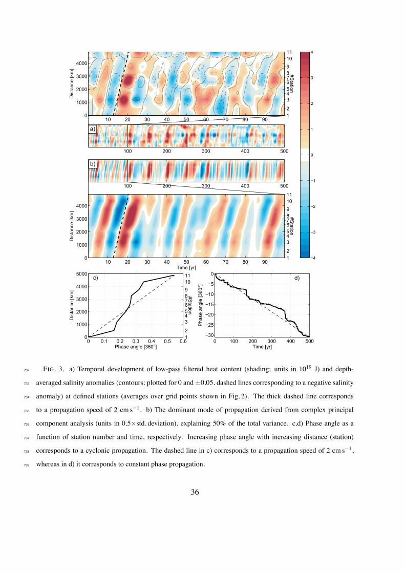
Fig. 3. a) Temporal development of low-pass filtered heat content (shading; units in 1019 J) and672
depth-averaged salinity anomalies (contours; plotted for 0 and ±0.05, dashed lines corre-673
sponding to a negative salinity anomaly) at defined stations (averages over grid points shown674
in Fig. 2). The thick dashed line corresponds to a propagation speed of 2 cm s−1. b) The675
dominant mode of propagation derived from complex principal component analysis (units676
in 0.5×std. deviation), explaining 50% of the total variance. c,d) Phase angle as a function677
of station number and time, respectively. Increasing phase angle with increasing distance678
(station) corresponds to a cyclonic propagation. The dashed line in c) corresponds to a679
propagation speed of 2 cm s−1, whereas in d) it corresponds to constant phase propagation. . . 36680
Fig. 4. Heat content (shading) and temperature (contours) variability (expressed as one standard681
deviation) at defined stations as a function of depth. The black line displays the average682
depth of the winter (December–April) mixed layer. . . . . . . . . . . . . 37683
Fig. 5. Power spectrum (thick lines) for a) heat content and b) salinity anomalies at St1 and St3684
based on unfiltered data together with the theoretical red noise spectrum (thin solid lines)685
computed by fitting a first order autoregressive process with a 95% confidence interval686
(thin dashed lines) around the red noise. c) Power spectrum for observed (HadISST) win-687
ter (December–April) sea surface temperatures in the Norwegian Sea (0.5–17.5◦E, 60.5–688
71.5◦N) between 1870 and 2013. Winter SST is considered because it represents the upper-689
ocean heat content as a result of a deep winter mixed layer. . . . . . . . . . . 38690
Fig. 6. a) Heat budget for the Norwegian Sea (low-pass filtered), where HCt is the heat content691
tendency, Qadv is the heat transport convergence, Qs is the net surface heat flux (positive out692
of the ocean), and Qres is a residual term. The domain (upper map) is bounded in the south693
by the Iceland–Scotland ridge and in the west and north by the extent of the Atlantic domain,694
visible by the gradient in heat content variability (expressed as one standard deviation; units695
in 108 Jm−2). The lower map displays the grid points used in the analysis. Colored circles696
and black dots present the ocean grid, while the red open squares are the atmospheric grid697
points used to analyze surface air temperature. b) Heat transport anomalies (HT ; low-pass698
filtered) through the vertical sections of the control volume. The line colors correspond to699
the section color given in the lower map and the names refer to geographic location or major700
currents. HTaw: Atlantic water; HTns: North Sea; HTgs: Greenland Sea; HTbs: Barents Sea;701
HTwsc: West Spitsbergen Current. . . . . . . . . . . . . . . . . . 39702
32

Fig. 7. Relative magnitude of oceanic (Qo = Qadv+Qres) and atmospheric (Qs) heat budget terms,703
calculated as std(Qo)/std(Qs) and presented on a log scale. Values >1 indicate that the704
oceanic contribution is the largest. . . . . . . . . . . . . . . . . . 40705
Fig. 8. Heat transport anomalies (low-pass filtered) between Iceland and Scotland (Fig. 6; HTaw)706
decomposed into a temperature component (vT ′), a velocity component (v′T ), and an eddy707
component (v′T ′). . . . . . . . . . . . . . . . . . . . . . 41708
Fig. 9. Power spectrum for a) surface heat flux (Qs) and surface air temperature (SAT) in the Nor-709
wegian Sea (cf. Fig. 6), and b) the heat transport between Iceland and Scotland (HTaw) and710
the strength of the subpolar gyre (SPG) based on unfiltered data. The red noise spectrums711
and 95% confidence intervals are also plotted (see Fig. 5 for description). The SPG strength712
is calculated as the absolute value of the minimum barotropic streamfunction in the subpolar713
region (Langehaug et al. 2012a). . . . . . . . . . . . . . . . . . 42714
Fig. 10. The influence of ocean heat transport into the Nordic Seas (HTaw; black circles) on a) surface715
heat flux to the atmosphere, b) sea ice concentration loss, and c) surface air temperature,716
based on linear regression analysis on low-pass filtered time series. The ocean heat transport717
leads by 2 years. Only regressions significant at the 95% confidence level are plotted. Units718
are given in Wm−2, %, and ◦C, respectively, per std(HTaw). . . . . . . . . . . 43719
33

24oW 12oW 0o 12oE 24oE
55oN
60oN
65oN
70oN
75oN
80oN
10 cm/s5 cm/s
b)
[°C]
2 0 2 4 6 8 10
24oW 12oW 0o 12oE 24oE
55oN
60oN
65oN
70oN
75oN
80oN a)
[°C]
2 0 2 4 6 8 10
BarentsSea
Norway
Iceland
Gre
enla
nd
Svalbard
NwAC
EGC
NorthAtlantic
GreenlandSea
NorwegianSea
WSC
DS
Fram Strait
Faroe Is
Scotland
Sh
RT
FIG. 1. a) Observed and b) modeled winter (December–April) upper-ocean temperature (shading) and sea ice
extent (white line; defined where the sea ice concentration is 15%) in the northern seas. Observations are from
HadISST (Rayner et al. 2003). The arrows indicate the main features of the near-surface circulation (NwAC:
Norwegian Atlantic Current; WSC: West Spitsbergen Current; EGC: East Greenland Current). Modeled tem-
perature and velocities are averages within the surface mixed layer (note the different velocity scales). Isobaths
are given every 1000 m (thin gray lines) and for 500 m depth (black line) which roughly marks the continental
slopes. DS: Denmark Strait; RT: Rockall Trough; Sh: Shetland.
720
721
722
723
724
725
726
34

20oW 10oW 0o 10oE 20oE 30oE
55oN
60oN
65oN
70oN
75oN
80oN
−3
−1.5
−2
−1.5St1
St2 St3
St4
St5
St6
St7
St8
St9
St10
St11
0 0.2 0.4 0.6 0.8 1
FIG. 2. Barotropic streamlines showing the mean cyclonic circulation within the northern seas (thick black
lines; plotted for -1.5 Sv, -2 Sv, and -3 Sv; 1 Sv≡ 106 m3 s−1). Isobaths are given for 500 m, 2000 m, and
3000 m depth (gray lines). The colored circles show the grid points used to define the path of ocean heat
anomalies, where the associated color indicates the maximum lagged correlation between adjacent stations, i.e.,
the correlation shown for St2 corresponds to r(St1,St2). Station numbers are assigned and used in the text.
727
728
729
730
731
35
100 200 300 400 500
Dis
tanc
e [k
m]
10 20 30 40 50 60 70 80 900
1000
2000
3000
4000
12
34567891011
#Station
−4
−3
−2
−1
0
1
2
3
4
Time [yr]
Dis
tanc
e [k
m]
10 20 30 40 50 60 70 80 900
1000
2000
3000
4000
12
34567891011
#Station
100 200 300 400 500
0 0.1 0.2 0.3 0.4 0.5 0.60
1000
2000
3000
4000
5000
Phase angle [360°]
Dis
tanc
e [k
m]
c)
12
34567891011
#Station
0 100 200 300 400 500−30
−25
−20
−15
−10
−5
0
Time [yr]
Pha
se a
ngle
[360
°]
d)
a)
b)
FIG. 3. a) Temporal development of low-pass filtered heat content (shading; units in 1019 J) and depth-
averaged salinity anomalies (contours; plotted for 0 and±0.05, dashed lines corresponding to a negative salinity
anomaly) at defined stations (averages over grid points shown in Fig. 2). The thick dashed line corresponds
to a propagation speed of 2 cm s−1. b) The dominant mode of propagation derived from complex principal
component analysis (units in 0.5×std. deviation), explaining 50% of the total variance. c,d) Phase angle as a
function of station number and time, respectively. Increasing phase angle with increasing distance (station)
corresponds to a cyclonic propagation. The dashed line in c) corresponds to a propagation speed of 2 cm s−1,
whereas in d) it corresponds to constant phase propagation.
732
733
734
735
736
737
738
739
36

#Station
Dep
th [m
]
0.2
0.2
0.2
0.4
0.4
0.4
0.6
0.6
0.6
0.8
0.8
0.8
1
1
1
1 2 3 4 5 6 7 8 9 10 11
100
200
300
400
500
600
700
800
900
1000
[109 J m−2]
0 0.5 1 1.5 2 2.5 3 3.5 4
FIG. 4. Heat content (shading) and temperature (contours) variability (expressed as one standard deviation) at
defined stations as a function of depth. The black line displays the average depth of the winter (December–April)
mixed layer.
740
741
742
37

5102030500
5
10
15
20
25
Period [yr]
|Y(f)
|
St3St1
a)
5102030500
5
10
15
20
25
Period [yr]
|Y(f)
|
St3St1
b)
5102030500
1
2
3
4
5
6
7
8
9
10
Period [yr]
|Y(f)
|
HadISST
c)
FIG. 5. Power spectrum (thick lines) for a) heat content and b) salinity anomalies at St1 and St3 based on
unfiltered data together with the theoretical red noise spectrum (thin solid lines) computed by fitting a first
order autoregressive process with a 95% confidence interval (thin dashed lines) around the red noise. c) Power
spectrum for observed (HadISST) winter (December–April) sea surface temperatures in the Norwegian Sea (0.5–
17.5◦E, 60.5–71.5◦N) between 1870 and 2013. Winter SST is considered because it represents the upper-ocean
heat content as a result of a deep winter mixed layer.
743
744
745
746
747
748
38

−80
−60
−40
−20
0
20
40
60
80
Hea
t ano
mal
y [T
W]
a) HCt = Qadv − Qs + Qres
10 20 30 40 50 60 70 80 90 100−100
−80
−60
−40
−20
0
20
40
60
80
100
Time [yrs]
Hea
t ano
mal
y [T
W]
b) Qadv = HTaw + HTns + HTgs + HTbs + HTwsc
0 1 2 3 4 5
FIG. 6. a) Heat budget for the Norwegian Sea (low-pass filtered), where HCt is the heat content tendency,
Qadv is the heat transport convergence, Qs is the net surface heat flux (positive out of the ocean), and Qres is a
residual term. The domain (upper map) is bounded in the south by the Iceland–Scotland ridge and in the west
and north by the extent of the Atlantic domain, visible by the gradient in heat content variability (expressed
as one standard deviation; units in 108 Jm−2). The lower map displays the grid points used in the analysis.
Colored circles and black dots present the ocean grid, while the red open squares are the atmospheric grid points
used to analyze surface air temperature. b) Heat transport anomalies (HT ; low-pass filtered) through the vertical
sections of the control volume. The line colors correspond to the section color given in the lower map and the
names refer to geographic location or major currents. HTaw: Atlantic water; HTns: North Sea; HTgs: Greenland
Sea; HTbs: Barents Sea; HTwsc: West Spitsbergen Current.
749
750
751
752
753
754
755
756
757
758
39

24oW 12oW 0o 12oE 24oE
55oN
60oN
65oN
70oN
75oN
80oN
0.5
1
2
4
8
FIG. 7. Relative magnitude of oceanic (Qo =Qadv+Qres) and atmospheric (Qs) heat budget terms, calculated
as std(Qo)/std(Qs) and presented on a log scale. Values >1 indicate that the oceanic contribution is the largest.
759
760
40

0 50 100 150 200 250 300 350 400 450 500−100
−50
0
50
100
Time [yrs]
Hea
t ano
mal
y [T
W]
HTaw = vT′ + v
′T + v
′T
′
FIG. 8. Heat transport anomalies (low-pass filtered) between Iceland and Scotland (Fig. 6; HTaw) decomposed
into a temperature component (vT ′), a velocity component (v′T ), and an eddy component (v′T ′).
761
762
41

5102030500
5
10
15
Period [yr]
|Y(f)
|
SAT
Qs
a)
5102030500
5
10
15
Period [yr]
|Y(f)
|SPG
HTaw
b)
FIG. 9. Power spectrum for a) surface heat flux (Qs) and surface air temperature (SAT) in the Norwegian
Sea (cf. Fig. 6), and b) the heat transport between Iceland and Scotland (HTaw) and the strength of the subpolar
gyre (SPG) based on unfiltered data. The red noise spectrums and 95% confidence intervals are also plotted
(see Fig. 5 for description). The SPG strength is calculated as the absolute value of the minimum barotropic
streamfunction in the subpolar region (Langehaug et al. 2012a).
763
764
765
766
767
42

a) 20oW 0o 20oE 40oE 60oE
55oN
60oN
65oN
70oN
75oN
80oN
0
2
4
6
8
10
12
14
16
b)
55oN
60oN
65oN
70oN
75oN
80oN
0
1
2
3
4
5
6
7
8
55oN
60oN
65oN
70oN
75oN
80oN c)
0
0.1
0.2
0.3
0.4
0.5
0.6
0.7
0.8
FIG. 10. The influence of ocean heat transport into the Nordic Seas (HTaw; black circles) on a) surface heat
flux to the atmosphere, b) sea ice concentration loss, and c) surface air temperature, based on linear regression
analysis on low-pass filtered time series. The ocean heat transport leads by 2 years. Only regressions significant
at the 95% confidence level are plotted. Units are given in Wm−2, %, and ◦C, respectively, per std(HTaw).
768
769
770
771
43