On analytical formulae for navigation lock filling ...On analytical formulae for navigation lock...
32
On analytical formulae for navigation lock filling-emptying and overtravel LAURENT SCHINDFESSEL, Ph.D. student, Hydraulics Laboratory, Department of Civil Engineering, Ghent University, Sint-Pietersnieuwstraat 41 B5, B-9000 Ghent, Belgium Email: [email protected] (author for correspondence) TOM DE MULDER (IAHR Member), Associate professor, Hydraulics Laboratory, Department of Civil Engineering, Ghent University, Sint-Pietersnieuwstraat 41 B5, B-9000 Ghent, Belgium Email: [email protected] STEPHAN CREELLE, Ph.D. student, Hydraulics Laboratory, Department of Civil Engineering, Ghent University, Sint-Pietersnieuwstraat 41 B5, B-9000 Ghent, Belgium Email: [email protected] GERALD A. SCHOHL (IAHR Member), Senior hydraulic expert, Retired from Tennessee Valley Authority Engineering Laboratory, Hydraulic Consultant, Knoxville, Tennessee Email: [email protected] Running Head: Navigation lock filling-emptying and overtravel formulae
Transcript of On analytical formulae for navigation lock filling ...On analytical formulae for navigation lock...
On analytical formulae for navigation lock filling-emptying and
overtravel
LAURENT SCHINDFESSEL, Ph.D. student, Hydraulics Laboratory, Department of Civil
Engineering, Ghent University, Sint-Pietersnieuwstraat 41 B5, B-9000 Ghent, Belgium
Email: [email protected] (author for correspondence)
TOM DE MULDER (IAHR Member), Associate professor, Hydraulics Laboratory,
Department of Civil Engineering, Ghent University, Sint-Pietersnieuwstraat 41 B5, B-9000
Ghent, Belgium
Email: [email protected]
STEPHAN CREELLE, Ph.D. student, Hydraulics Laboratory, Department of Civil
Engineering, Ghent University, Sint-Pietersnieuwstraat 41 B5, B-9000 Ghent, Belgium
Email: [email protected]
GERALD A. SCHOHL (IAHR Member), Senior hydraulic expert, Retired from Tennessee
Valley Authority Engineering Laboratory, Hydraulic Consultant, Knoxville, Tennessee
Email: [email protected]
Running Head: Navigation lock filling-emptying and overtravel formulae
On analytical formulae for navigation lock filling-emptying and
overtravel
ABSTRACT
In culvert-based navigation lock filling-emptying systems, inertia effects have a significant influence
on the filling-emptying time and cause a (damped) oscillation of the water surface in the lock chamber
around its equalization level, referred to as the overtravel phenomenon. In this paper, the derivation of
analytical formulae for the lock filling-emptying time and overtravel peak of systems consisting of a
number of identical culverts is revisited. In comparison to earlier publications, the underlying
assumptions are made explicit and the importance of accounting for the surface area ratio of lock
chamber to upper reservoir in case of filling (resp. lower reservoir in case of emptying) is pointed out.
Additionally, it is shown how the applicability of the analytical formulae can be extended to lock
filling-emptying systems with more complex lay-outs by using an “equivalent culvert” approach. The
validity of the analytical formulae is thoroughly assessed, first by comparing to an accurate numerical
solution of the governing non-linear second-order differential equations, and secondly, by means of
experiments in a physical model.
Keywords: culvert; filling time; inertia; navigation lock; overtravel
1. Introduction
Several types of navigation lock filling and emptying systems exist, many of which make use
of culverts to transfer water by gravity from an upper reservoir to the lock chamber in case of
filling, or from the lock chamber to a lower reservoir in case of emptying, see e.g. PIANC
(1986). In a system with bypass (or looped) culverts in the lock head, the culverts are
relatively short in comparison to the lock chamber length, whereas in a sidewall filling system
with ports, the longitudinal culverts are relatively long. Various other types of culvert-based
systems exist, making use of different combinations of longitudinal culverts (in the sidewalls
or central in the chamber) and lateral culverts on top of or under the lock chamber floor.
In the hydraulic design of a navigation lock filling and emptying system, the lock
filling or emptying time is a key parameter, which should remain below a specified threshold
value (without causing an inconvenient level of turbulence in the lock chamber). Besides
numerical modelling and physical modelling, also analytical formulae are still useful as
design tools nowadays, especially in the early stages of design.
For a simple through-the-gate system consisting of valves in the lock gates - i.e. not
making use of culverts - an analytical formula for the filling (resp. emptying) time can be
derived in a straightforward way. This classical formula has been, and still is, also applied to
culvert-based systems.
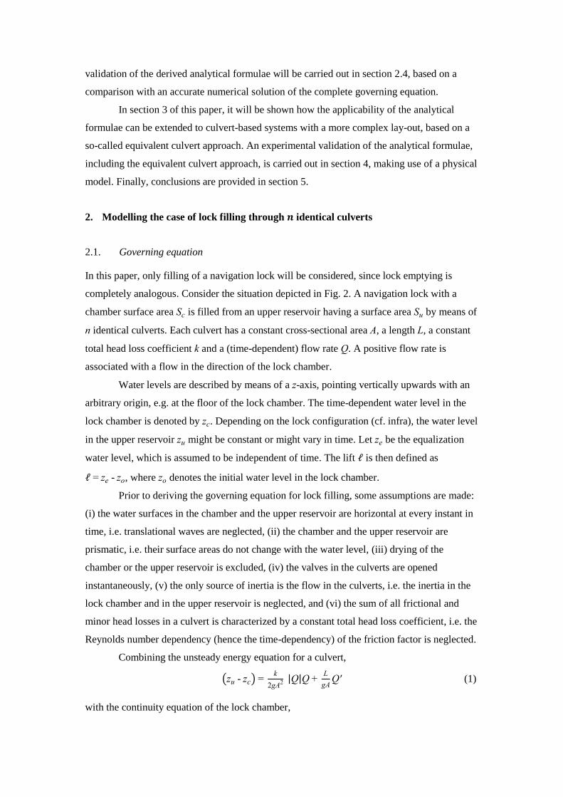
For a culvert-based system in a lock of the Panama Canal, however, it was noted in
Pillsbury (1915) that lock filling does not exactly follow the classical formula and that, at the
end of filling the water level in the lock chamber tends to rise above the level of the upper
reservoir. For emptying, an analogous behaviour is observed. This phenomenon is referred to
as overtravel and is characterized by a damped oscillation of the water surface in the lock
chamber with respect to its equalization level, as is schematically shown in Fig. 1. Pillsbury
(1915) attributed these features to the inertia of the water flowing in the culverts and derived
an approximate formula for the lock filling (or emptying) time, containing the height of the
first overtravel peak as a parameter. The Pillsbury formula appears e.g. in Dehousse (1985)
and USACE (2006). The latter reference also provides, without explicit derivation, an
analytical formula for the height of the first overtravel peak. Dehousse (1985) on the other
hand, does provide a derivation for the height of the first three overtravel peaks.
In section 2 of this paper, the derivation of the aforementioned analytical formulae
will be revisited, in order to clarify the underlying assumptions and approximations, and
possibly extend their scope. It will turn out that these formulae assume a lock filling (and
emptying) system consisting of a number of identical culverts.
The governing equation is a non-linear second-order differential equation, containing
a quadratic damping term (section 2.1). Such an equation is generic to many problems in
hydraulics. It describes e.g. also the water level behaviour in a surge tank of a hydropower
conveyance system. In the latter field of application, the overtravel phenomenon and its
governing equation have already been studied to some depth; see e.g. Jaeger (1956), Reisman
& Silvers (1967) and Steber & Reisman (1969). This is beneficial for the study of overtravel
in navigation lock filling, allowing some insight and modelling approaches to be shared. Yet,
navigation lock filling and overtravel deserves a study in itself, given the large ratio of
chamber surface area to cross-sectional area of the feeding culvert and the different initial
conditions, as compared to surge tanks.
Even when the damping parameter is assumed to be a constant, no exact closed form
solution of the governing differential equation is known to date. In section 2.2, an
approximate solution of the complete equation will be derived, in a similar way as proposed
by Pillsbury (1915), yielding analytical formulae for the lock filling time, the height of the
first overtravel peak and a typical frequency of the water level oscillations around the
equalization level. The formulae derived in this paper will also apply to lock filling (or
emptying) configurations in which the surface area of the upper (or lower) reservoir is not
infinitely large in comparison to the one of the lock chamber, an assumption which is often
implicitly made in earlier publications. Some alternative analytical formulae will be derived
in section 2.3 as exact solutions to simplified forms of the governing equation. A numerical
validation of the derived analytical formulae will be carried out in section 2.4, based on a
comparison with an accurate numerical solution of the complete governing equation.
In section 3 of this paper, it will be shown how the applicability of the analytical
formulae can be extended to culvert-based systems with a more complex lay-out, based on a
so-called equivalent culvert approach. An experimental validation of the analytical formulae,
including the equivalent culvert approach, is carried out in section 4, making use of a physical
model. Finally, conclusions are provided in section 5.
2. Modelling the case of lock filling through 𝒏 identical culverts
2.1. Governing equation
In this paper, only filling of a navigation lock will be considered, since lock emptying is
completely analogous. Consider the situation depicted in Fig. 2. A navigation lock with a
chamber surface area Sc is filled from an upper reservoir having a surface area Su by means of
n identical culverts. Each culvert has a constant cross-sectional area A, a length L, a constant
total head loss coefficient k and a (time-dependent) flow rate Q. A positive flow rate is
associated with a flow in the direction of the lock chamber.
Water levels are described by means of a z-axis, pointing vertically upwards with an
arbitrary origin, e.g. at the floor of the lock chamber. The time-dependent water level in the
lock chamber is denoted by zc. Depending on the lock configuration (cf. infra), the water level
in the upper reservoir zu might be constant or might vary in time. Let ze be the equalization
water level, which is assumed to be independent of time. The lift ℓ is then defined as
ℓ = ze - zo, where zo denotes the initial water level in the lock chamber.
Prior to deriving the governing equation for lock filling, some assumptions are made:
(i) the water surfaces in the chamber and the upper reservoir are horizontal at every instant in
time, i.e. translational waves are neglected, (ii) the chamber and the upper reservoir are
prismatic, i.e. their surface areas do not change with the water level, (iii) drying of the
chamber or the upper reservoir is excluded, (iv) the valves in the culverts are opened
instantaneously, (v) the only source of inertia is the flow in the culverts, i.e. the inertia in the
lock chamber and in the upper reservoir is neglected, and (vi) the sum of all frictional and
minor head losses in a culvert is characterized by a constant total head loss coefficient, i.e. the
Reynolds number dependency (hence the time-dependency) of the friction factor is neglected.
Combining the unsteady energy equation for a culvert,
(zu - zc) = k
2gA2 |Q|Q +
L
gAQ' (1)
with the continuity equation of the lock chamber,
Sczc' = nQ (2)
and the mass balance between the upper reservoir and the chamber,
(zu - ze)Su = (ze - zc)Sc (3)
yields the following second-order differential equation:
(1 + Sc
Su) (zc - ze) +
k
2g(
Sc
nA)
2
|zc' |zc
' + L
g(
Sc
nA) zc
'' = 0 (4)
where the prime denotes a derivative with respect to time t. The initial conditions are:
zc = zo(= ze - ℓ) and zc' = 0 at t = 0 (5)
Note that Eq. (3) expresses that the upper reservoir and the lock chamber act as
communicating vessels. As a consequence, the water level in the upper reservoir zu might
vary in time because of filling of the lock chamber. All other causes of time-dependency of zu
(like e.g. tidal waves, translation waves, etc.) are neglected in this paper, in order for the
equalization level ze to be constant in time.
By introducing an inverse time scale ωo,
ωo = (gnA
LSc)
12 (6)
a dimensionless time coordinate τ can be defined as τ = ωot. Similarly, the deviation of the
(time-dependent) water surface in the lock chamber from its equalization level can be
presented by the dimensionless parameter ζ:
ζ = zc - ze
ℓ (7)
where zc is a function of time t, and ζ is a function of dimensionless time τ = ωot.
Equation (4) can now be rewritten in dimensionless form:
(1 + σ)ζ + ψ|ζ|ζ + ζ = 0 (8)
where a dot represents a derivative with respect to τ, σ denotes the ratio of the surface areas,
i.e. σ = Sc/Su, while ψ is a dimensionless damping parameter:
ψ = k
2
ℓ
L
Sc
nA (9)
In dimensionless form, the initial conditions of Eq. (5) become:
ζ = -1 and ζ = 0 at τ = 0 (10)
The parameter σ is a positive constant that depends on the configuration of the
navigation lock. If the surface area of the upper reservoir Su is infinitely large (in comparison
to the surface area of the lock chamber Sc), then σ = 0. This situation is typical for filling a
lock chamber from a (long) river or canal reach (with a large forebay). The case of a staircase
lock, where relatively short reaches are present between consecutive lock chambers,
corresponds to the range 0 < σ < 1. In case of a double-lift lock, both chambers have an equal
surface area, and σ equals 1. From Eq. (3) it follows that the case σ = 0 is equivalent to zu
being constant in time (and equal to the equalization level ze). For all other values of the σ
parameter, lock filling will give rise to zu varying in time, though the equalization level ze is
constant in time.
Unless stated otherwise, both damping and culvert inertia are taken into account in
this paper. The corresponding non-linear second-order differential Eq. (8) is referred to as the
complete governing equation, which needs to be solved in combination with Eq. (10). The
governing equation is said to be simplified when either damping or inertia is neglected.
2.2. Analytical formulae derived from approximate solution of complete equation
Similar to other quadratically damped hydraulic systems mentioned in the introduction, no
exact analytical solution of the governing equation (8) and initial conditions (10) seems
possible when both damping and inertia are accounted for.
A first integration of Eq. (8) in the time interval that ζ is positive (i.e. from the start of
filling at τ = 0 till the moment that the first overtravel peak is reached at τ = τ1) yields:
(ζ) 2 = 1 + σ
2ψ2 -
1 + σ
ψζ- (
1 + σ
2ψ2 +
1 + σ
ψ) exp{-2ψ(ζ + 1)} (11)
As was already conjectured by Pillsbury (1915) and will be demonstrated below, the
exponential term in Eq. (11) can often be neglected in good approximation for many culvert-
based lock filling-emptying systems. Further integration then yields:
ζ = 1
2ψ - [(
1
2ψ + 1)
12
- 1
2(
1 + σ
ψ)
12τ]
2
(12)
Equation (12) allows derivation of approximate analytical formulae (see table 1, formulae
with a Roman numeral I followed by a letter) for the most important navigation lock filling
parameters (Fig. 1) in dimensionless form: (i) the filling time τfull (= ωotfull), (ii) the water
surface deviation from the equalization level at the first overtravel peak ζ1 (= (z1 - ze) ℓ⁄ ),
(iii) the time of the first overtravel peak τ1 (= ωot1) and (iv) an approximate frequency of the
chamber surface oscillations around the equalization level during the overtravel phenomenon
Ω (= ω/ωo). Note that due to the non-linear damping in the system, the frequency content of
those oscillations will change in time. At the onset of the overtravel phenomenon, the basic
frequency of the oscillations is ω = 2π/Tosc
, where Tosc is the time interval between the first
two up-crossings of the equalization level in the chamber (see Fig. 1). When deriving the
expression for Ω in table 1, the following approximation has been made:
Tosc ≈ 4(t1 - tfull), hence Ω ≈ π 2⁄
(τ1 - τfull) (13)
Note that table 1 also contains formulae (with a Roman numeral II followed by a
letter) which are valid for the special case when the surface area of the upper reservoir is
infinitely large (in comparison to the lock chamber surface) and which are retrieved by simply
putting σ = 0 in the general formulae. As mentioned before, this special case is typically
associated to navigation locks being filled from a river or channel reach (with a large
forebay).
Formula (IIb) of the present paper (table 1), regarding the filling time, has been
presented earlier as formula (5-5) in USACE (2006) and goes back to the formula derived by
Pillsbury (1915). Similarly, formula (IIc) for the water level at the first overtravel peak in
table 1 has been presented (without explicit derivation) earlier as formula (5-20) in USACE
(2006). Formulae similar to (IIb) and (IIc) have also been derived in Dehousse (1985). From
the foregoing, it follows that the earlier presented formulae are only valid for the special case
of an infinitely large surface of the upper reservoir, though this was not clearly stated in the
cited references. The present paper offers formulae, like e.g. (Ib) and (Ic), which have a
broader range of applicability than the formulae presented earlier in literature. For the sake of
completeness, however, it should be mentioned that Pillsbury (1915) briefly points out how
his lock filling time formula should be modified in case of locks in flight, but without
providing a complete derivation.
Note that the formulae in table 1 were derived based on the assumption that the
culvert valves open instantaneously, i.e. assuming a zero value for the valve opening time tv.
In practice, this is not feasible (since it would imply an infinite lift force) nor desirable (since
it would lead to large surge waves in the lock chamber). In case of a finite opening time of the
valves, the lock chamber will fill more slowly. Therefore, it is expected that the formulae (Ic)
or (IIc) for the height of the first overtravel peak will lead to overestimates. Regarding the
filling time, it is proposed in USACE (2006) to add a term Ktv, where K is an overall valve
coefficient (in the range 0.4 to 0.6), to the analytical formula for the filling time tfull in case of
instantaneous opening of the culvert valves. In the dimensionless formulation of the present
paper, this would lead to adding a term Kωotv to the right hand side of formulae (Ib) and (IIb)
in table 1.
2.3. Analytical formulae derived from exact solution of simplified equation
In this section, some additional formulae will be presented in order to gain some more
(physical) insight and for comparison purposes (see sections 2.4 and 4.5) with the formulae
derived in section 2.2.
A first simplification of the governing equation that leads to an exact solution,
consists in neglecting damping but still accounting for inertia, i.e. ψ = 0. Then, Eq. (8) reduces
to a linear second-order differential equation, (1 + σ)ζ + ζ = 0, which combined with the initial
conditions in Eq. (10) leads to the solution:
ζ = - cos [(1 + σ)12 τ] = - cos [(1 + σ)
12 ωot] (14)
The analytical formulae for the filling time and overtravel characteristics that can be derived
from Eq. (14) are presented in table 2 (i.e. formulae with a Roman numeral III followed by a
letter). From Eq. (14) it can be deduced that the inverse time scale ωo – by means of which
the dimensionless time coordinate τ is defined (Eq. (6)) – corresponds to the frequency of the
chamber surface oscillations around the equalization level in case of an undamped system
with an infinitely large surface area of the upper reservoir, i.e. if ψ = σ = 0.
A second simplification of the governing equation that is considered, consists in
neglecting inertia but still accounting for damping. When inertia is neglected, the ζ term
disappears from Eq. (8), which in combination with the initial conditions of Eq. (10) yields an
exact solution:
ζ = [1 - 1
2(
1 + σ
ψ)
1
2τ]
2
(15)
The analytical formula for the filling time that can be derived from Eq. (15) is presented as
formula (IVb) in table 2. Since no overtravel takes place in an inertialess configuration, table
2 contains no formulae for the overtravel characteristics. Note that for the special case of an
inertialess system with an infinitely large surface area of the upper reservoir, i.e. if σ = 0,
formula (IVb) in table 2 reduces to:
τfull = 2ψ12 (16)
Converting Eq. (16) for the dimensionless filling time τfull (= ωotfull) to physical dimensions,
by substituting the expressions for ωo = (gnA
LSc)
12 and ψ =
k
2
ℓ
L
Sc
nA, yields:
tfull = 2Sc√ℓ
CLnA√2g (17)
where the overall lock coefficient CL is defined as in USACE (2006), CL= 1 √k⁄ .
Equation (17) is a classical formula in textbooks on navigation locks (like e.g.
Dehnert (1954)), since it is straightforward to derive for a simple through-the-gate filling-
emptying system based upon valves in the lock gates. The latter system can be interpreted as
an inertialess limit case of a culvert-based system, i.e. a system in which the culvert length
L→0. Strictly speaking, this limit case would result in both ωo→∞ and ψ→∞. Since the
culvert length has no physical meaning any more for a through-the-gate system, any non-zero
length scale L can be used to define both ωo and ψ. Note that the choice of the length scale is
not relevant, since the L appearing in the expression for ωo and the one appearing in the
expression for ψ cancel against each other, yielding formula (17) which is independent of L.
Note that Eq. (17), which is derived from Eq. (16) and is valid for an inertialess
system (with σ = 0), states that the lock filling time is inversely proportional to the number n
of identical culverts. This implies that doubling the number of culverts (i.e. filling openings in
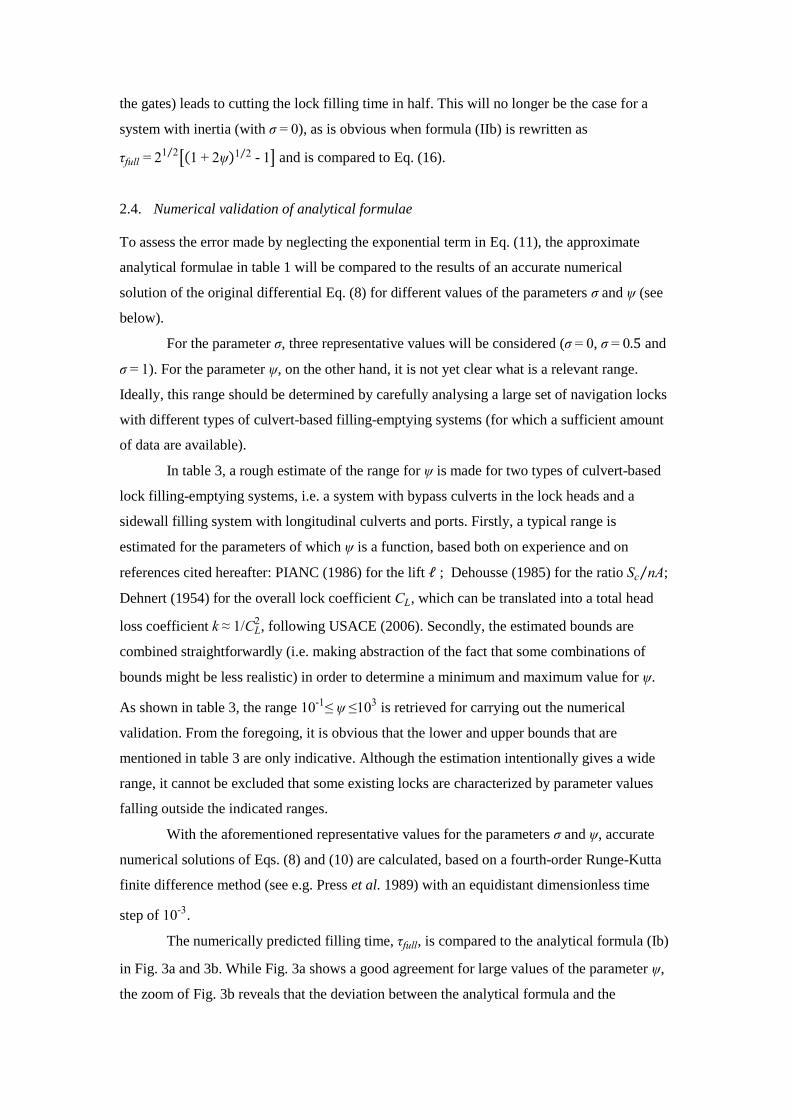
the gates) leads to cutting the lock filling time in half. This will no longer be the case for a
system with inertia (with σ = 0), as is obvious when formula (IIb) is rewritten as
τfull = 21 2⁄ [(1 + 2ψ)1 2⁄ - 1] and is compared to Eq. (16).
2.4. Numerical validation of analytical formulae
To assess the error made by neglecting the exponential term in Eq. (11), the approximate
analytical formulae in table 1 will be compared to the results of an accurate numerical
solution of the original differential Eq. (8) for different values of the parameters σ and ψ (see
below).
For the parameter σ, three representative values will be considered (σ = 0, σ = 0.5 and
σ = 1). For the parameter ψ, on the other hand, it is not yet clear what is a relevant range.
Ideally, this range should be determined by carefully analysing a large set of navigation locks
with different types of culvert-based filling-emptying systems (for which a sufficient amount
of data are available).
In table 3, a rough estimate of the range for ψ is made for two types of culvert-based
lock filling-emptying systems, i.e. a system with bypass culverts in the lock heads and a
sidewall filling system with longitudinal culverts and ports. Firstly, a typical range is
estimated for the parameters of which ψ is a function, based both on experience and on
references cited hereafter: PIANC (1986) for the lift ℓ ; Dehousse (1985) for the ratio Sc nA⁄ ;
Dehnert (1954) for the overall lock coefficient CL, which can be translated into a total head
loss coefficient k ≈ 1/CL2, following USACE (2006). Secondly, the estimated bounds are
combined straightforwardly (i.e. making abstraction of the fact that some combinations of
bounds might be less realistic) in order to determine a minimum and maximum value for ψ.
As shown in table 3, the range 10-1≤ ψ ≤103 is retrieved for carrying out the numerical
validation. From the foregoing, it is obvious that the lower and upper bounds that are
mentioned in table 3 are only indicative. Although the estimation intentionally gives a wide
range, it cannot be excluded that some existing locks are characterized by parameter values
falling outside the indicated ranges.
With the aforementioned representative values for the parameters σ and ψ, accurate
numerical solutions of Eqs. (8) and (10) are calculated, based on a fourth-order Runge-Kutta
finite difference method (see e.g. Press et al. 1989) with an equidistant dimensionless time
step of 10-3.
The numerically predicted filling time, τfull, is compared to the analytical formula (Ib)
in Fig. 3a and 3b. While Fig. 3a shows a good agreement for large values of the parameter ψ,
the zoom of Fig. 3b reveals that the deviation between the analytical formula and the
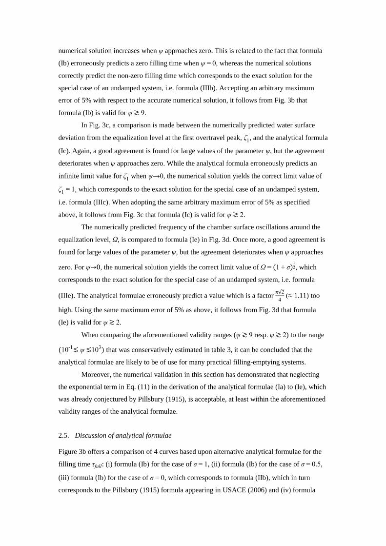
numerical solution increases when ψ approaches zero. This is related to the fact that formula
(Ib) erroneously predicts a zero filling time when ψ = 0, whereas the numerical solutions
correctly predict the non-zero filling time which corresponds to the exact solution for the
special case of an undamped system, i.e. formula (IIIb). Accepting an arbitrary maximum
error of 5% with respect to the accurate numerical solution, it follows from Fig. 3b that
formula (Ib) is valid for ψ ≳ 9.
In Fig. 3c, a comparison is made between the numerically predicted water surface
deviation from the equalization level at the first overtravel peak, ζ1, and the analytical formula
(Ic). Again, a good agreement is found for large values of the parameter ψ, but the agreement
deteriorates when ψ approaches zero. While the analytical formula erroneously predicts an
infinite limit value for ζ1 when ψ→0, the numerical solution yields the correct limit value of
ζ1 = 1, which corresponds to the exact solution for the special case of an undamped system,
i.e. formula (IIIc). When adopting the same arbitrary maximum error of 5% as specified
above, it follows from Fig. 3c that formula (Ic) is valid for ψ ≳ 2.
The numerically predicted frequency of the chamber surface oscillations around the
equalization level, Ω, is compared to formula (Ie) in Fig. 3d. Once more, a good agreement is
found for large values of the parameter ψ, but the agreement deteriorates when ψ approaches
zero. For ψ→0, the numerical solution yields the correct limit value of Ω = (1 + σ)12, which
corresponds to the exact solution for the special case of an undamped system, i.e. formula
(IIIe). The analytical formulae erroneously predict a value which is a factor π√2
4 (≈ 1.11) too
high. Using the same maximum error of 5% as above, it follows from Fig. 3d that formula
(Ie) is valid for ψ ≳ 2.
When comparing the aforementioned validity ranges (ψ ≳ 9 resp. ψ ≳ 2) to the range
(10-1≲ ψ ≲103) that was conservatively estimated in table 3, it can be concluded that the
analytical formulae are likely to be of use for many practical filling-emptying systems.
Moreover, the numerical validation in this section has demonstrated that neglecting
the exponential term in Eq. (11) in the derivation of the analytical formulae (Ia) to (Ie), which
was already conjectured by Pillsbury (1915), is acceptable, at least within the aforementioned
validity ranges of the analytical formulae.
2.5. Discussion of analytical formulae
Figure 3b offers a comparison of 4 curves based upon alternative analytical formulae for the
filling time τfull: (i) formula (Ib) for the case of σ = 1, (ii) formula (Ib) for the case of σ = 0.5,
(iii) formula (Ib) for the case of σ = 0, which corresponds to formula (IIb), which in turn
corresponds to the Pillsbury (1915) formula appearing in USACE (2006) and (iv) formula
(16), which corresponds to formula (IVb) for the special case of an inertialess configuration
with σ = 0.
Note that the predicted filling times of the four curves differ significantly, hence care
should be exercised when selecting an appropriate analytical formula for the filling time in a
given navigation lock configuration.
For a configuration with finite surface area for the upper reservoir, i.e. σ ≠ 0, it is
worth using formula (Ib) derived in this paper instead of the Pillsbury formula in USACE
(2006), as can be deduced from Fig. 3b. The Pillsbury formula is only appropriate for a
configuration with σ = 0.
Formula (16) - of which the dimensional form (17) is ubiquitous in textbooks and is
only valid for an inertialess configuration, like e.g. a through-the-gate system, in case σ = 0 -
results in a significant overprediction of the filling time for culvert-based systems. Hence,
formula (16) is in general not advocated for the latter type of filling-emptying systems,
though some practitioners do use it because of its simplicity. Yet, it is worth pointing out that
in case of σ = 0, formula (Ib) can be written as τfull = 21 2⁄ [(1+2ψ)1 2⁄ -1], from which it is
obvious that for large ψ values, the predictions of formula (Ib) approach the ones of formula
(16). The latter can indeed be observed in Fig. 3a.
With regard to the first overtravel peak relative to the equalization level, ζ1, Fig. 3c
only shows one curve which is based on an analytical formula, i.e. formula (Ic). Note that this
formula, which is identical to a formula appearing in USACE (2006), is independent of the
parameter σ.
As far as the dimensionless frequency Ω of the chamber surface oscillations around
the equalization level is concerned, it is worth mentioning that most references in literature,
like e.g. USACE (2006), contain no explicit analytical formula for this quantity. Figure 3d
offers a comparison of 3 curves based upon a single analytical formula that was derived in
this paper, i.e. formula (Ie). The three curves correspond to different values for σ: (i) σ = 1, (ii)
σ = 0.5 and (iii) σ = 0. Similar to the situation with respect to τfull, it is worth taking the
dimensions of the upper reservoir into account when predicting Ω (Fig. 3d).
3. Extension to more complex culvert geometries: equivalent culvert approach
While the aforementioned formulae were derived for the case of n identical culverts with
constant cross section, culvert-based lock filling-emptying systems often have a more
complex geometry. Some examples are: (i) culverts with cross-sectional changes, (ii) non-
identical bypass culverts in lock heads with rolling or sliding gates and (iii) systems of
(longitudinal) culverts with ports. Each of these systems can be modelled in good
approximation as a hydraulic network of pipes with constant cross section. As will be
explained below, every two pipes in the network that are connected in series can be
substituted by one equivalent culvert. The same goes for every two pipes in the network that
are connected in parallel. By repetitively applying these substitutions, any of the
aforementioned culvert-based systems can be ultimately modelled by means of one (n = 1)
equivalent culvert with constant cross section. This will allow application of the analytical
formulae derived earlier for the case of n identical culverts with constant cross section.
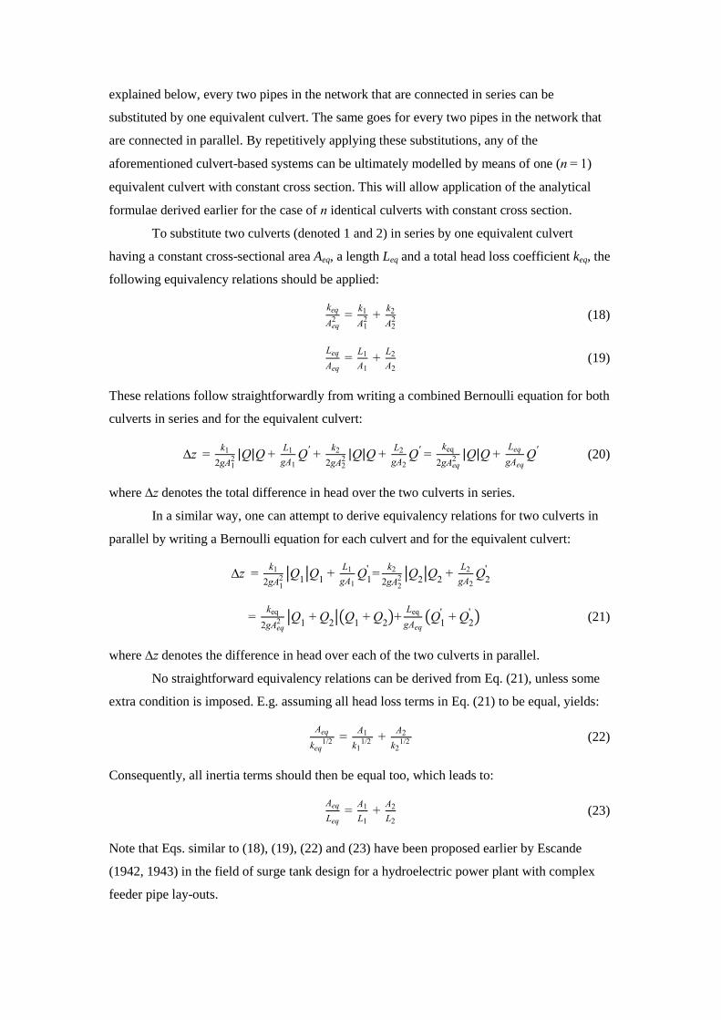
To substitute two culverts (denoted 1 and 2) in series by one equivalent culvert
having a constant cross-sectional area Aeq, a length Leq and a total head loss coefficient keq, the
following equivalency relations should be applied:
keq
Aeq2 =
k1
A12 +
k2
A22 (18)
Leq
Aeq =
L1
A1 +
L2
A2 (19)
These relations follow straightforwardly from writing a combined Bernoulli equation for both
culverts in series and for the equivalent culvert:
∆z = k1
2gA12 |Q|Q +
L1
gA1Q' +
k2
2gA22 |Q|Q +
L2
gA2Q' =
keq
2gAeq2 |Q|Q +
Leq
gAeqQ' (20)
where ∆z denotes the total difference in head over the two culverts in series.
In a similar way, one can attempt to derive equivalency relations for two culverts in
parallel by writing a Bernoulli equation for each culvert and for the equivalent culvert:
∆z = k1
2gA12 |Q
1|Q
1 +
L1
gA1Q
1' =
k2
2gA22 |Q
2|Q
2 +
L2
gA2Q
2'
= keq
2gAeq2 |Q
1 + Q
2|(Q
1 + Q
2)+
Leq
gAeq(Q
1' + Q
2' ) (21)
where ∆z denotes the difference in head over each of the two culverts in parallel.
No straightforward equivalency relations can be derived from Eq. (21), unless some
extra condition is imposed. E.g. assuming all head loss terms in Eq. (21) to be equal, yields:
Aeq
keq1/2 =
A1
k11/2 +
A2
k21/2 (22)
Consequently, all inertia terms should then be equal too, which leads to:
Aeq
Leq =
A1
L1 +
A2
L2 (23)
Note that Eqs. similar to (18), (19), (22) and (23) have been proposed earlier by Escande
(1942, 1943) in the field of surge tank design for a hydroelectric power plant with complex
feeder pipe lay-outs.

Since there are two equivalency relations defining the three parameters of the
equivalent culvert, one parameter can be chosen freely, e.g. Aeq.
With the equivalent culvert approach, a complex lock filling-emptying system can
ultimately be replaced by one single equivalent culvert. The corresponding governing
equation for the dimensionless water level in the lock chamber ζ, function of the
dimensionless time τ, can then be written as follows:
(1 + σ)ζ + ψeq
|ζ|ζ + ζ = 0 (24)
where
ψeq
= keq
2
ℓ
Leq
Sc
neqAeq (25)
and
τ = ωo,eqt = (gneqAeq
LeqSc)
12
t (26)
with neq = 1.
As a consequence, the analytical formulae in table 1 and their range of validity remain
applicable upon substituting ψ by ψeq
.
Note that for predicting lock characteristics other than those mentioned in table 1 - for
example, the distribution of the filling (or emptying) discharges and the associated surge
waves in the lock chamber - replacement of a (complex) filling-emptying system with one
equivalent culvert may not always be an adequate modelling strategy.
4. Experimental validation of analytical formulae
To assess the validity of the approximate analytical solutions of the complete equation, an
experimental validation is carried out. The experimental set-up and methodology will be
explained first. Then the application of the analytical formulae will be discussed.
Additionally, some numerical simulation work with a hydraulic network model will be
introduced. Finally, the analytical and numerical predictions will be compared with the
experimental results.
4.1. Experimental set-up and methodology
Figure 4 presents a schematic plan view of the experimental set-up, with the most important
dimensions. More details can be found in Schindfessel (2013). Two prismatic reservoirs, i.e.
the upper reservoir (with a surface area Su = 7.53 m²) and the lock chamber (with a surface
area Sc = 2.45 m²), are connected by culverts. Each culvert is sealed by a vertical lift valve.
All valves are opened manually in a nearly synchronous and instantaneous way.

In a first series of lock filling tests, both reservoirs merely act as communicating
vessels. These tests will be referred to as experiments with a finite upper reservoir,
characterized by a value of σ = Sc Su⁄ = 0.325. In a second series of tests, it is attempted to
keep the water level in the upper reservoir zu constant in time, by constantly adding discharge
to the upper reservoir while allowing the excess discharge to be drained over a spillway
construction. Such a configuration corresponds to the case of an infinitely large surface area
of the upper reservoir, hence σ = 0. Due to the limited size of the spillway, however, still a
(limited) variation in time of zu is observed in these tests. Therefore, the second series of tests
will be referred to as tests with a quasi infinite upper reservoir, denoted as σ ≈ 0.
In both series of tests, two distinct types of lock filling systems will be implemented.
The first type concerns systems which consist of n (= 1 or 2) identical culverts in parallel,
allowing a direct comparison of the experimental results with the analytical formulae derived
in section 2.2. The second type consists of systems which require the equivalent culvert
approach of section 3 to be applied, before a comparison of analytical results and
measurements is feasible.
For the first type of systems, culverts with three different lengths will be considered.
In table 4 (and subsequent tables), each of those systems will get a unique identifier
consisting of the number of identical culverts (i.e. n) followed by two characters
corresponding to the length of the culvert: short culvert (SC), medium length culvert (MC)
and long culvert (LC).
For the second type of systems, either systems composed of two bypass culverts with
different lengths (e.g. 1SC+1MC) will be considered or systems consisting of one
longitudinal culvert with ports (e.g. 1MC with 2 ports). Note in table 4 that, though not
strictly necessary, also system 2MC will be modelled with the equivalent culvert approach,
for comparison purposes with the results based upon the n identical culverts model.
All culverts in the aforementioned lock filling systems are implemented in the model
in a modular way by means of plastic (polyvinyl chloride, PVC) components (i.e. straight
pipes, bends, T-junctions, etc.) having a constant diameter (D = 0.1036 m), hence a constant
cross-sectional area (A = 8.43 10-3
m²).
An overview of the parameters characterizing the different lock-filling systems is
given in table 4. The k values in the table will be discussed in section 4.2. Note that different
values for the lift have been used for the case of a quasi infinite upper reservoir (ℓ ≈ 0.275 m,
with one exception, i.e. the system referred to as “1LC reduced lift”, for which ℓ ≈ 0.138 m)
and for the finite upper reservoir case (ℓ ≈ 0.185 m, except for 1LC reduced lift, for which
ℓ ≈ 0.082 m).

During the lock filling tests, water heights in the upper reservoir and in the lock
chamber are measured with two Cerabar S pressure sensors, having a measurement accuracy
of 0.5 mm according to the technical specifications. Both sensors are connected to an Arduino
micro-controller board, which is logging at a rate of 10 Hz. The measurement location of the
pressure sensor in the upper reservoir is fixed, whereas the sensor in the lock chamber can be
mounted in four alternative locations, as is schematically indicated in Fig. 4. The
measurement devices are calibrated, and each time they are moved, a reference water height is
read by means of a point gauge.
A given lock filling test is repeated several times, such that at least two measurements
are carried out in each of the alternative locations, to ensure that the average lock filling curve
(i.e. the arithmetic average of the individual, validated lock filling curves) is representative.
From the average filling curve, the lock filling time tfull, the height of the first overtravel peak
(z1 - ze) and the frequency of the chamber surface oscillations around the equalization level ω
are derived and reported in tables 5, 6 and 7, respectively.
The water level measurements are judged to be reproducible, since the individual lock
filling curves agree well. Moreover, it can be deduced from Fig. 5 that the individual heights
of the first overtravel peak (z1 - ze) only show a limited scatter around the reported one (i.e.
the value derived from the average lock filling curve) of about ± 1 mm.
Besides the unsteady lock filling tests, also some steady state experiments have been
run, in order to empirically derive the head loss characteristics of the distinct culverts. Those
runs are characterized by constant water levels in both the upper reservoir and the lock
chamber. The latter requires the water entering the lock chamber through the culverts to be
evacuated via an extra opening in the downstream wall of the lock chamber, sealed by a valve
(see Fig. 4).
4.2. Analytical predictions
The analytical formulae from table 1 require the parameter ψ (or ψeq) to be known, which in
turn requires estimates to be available for the total head loss coefficient 𝑘 of the distinct
culverts.
Though 𝑘 is meant to be a global coefficient for a lock filling system, it was
determined by modelling a given culvert first as a hydraulic network consisting of pipes (i.e.
frictional head losses) and resistances (i.e. minor head losses). Such an approach is also
advocated in USACE (2006).
To set up and numerically simulate the hydraulic network models, the LOCKSIM
software package developed by Schohl (1998) is used. LOCKSIM uses an explicit
approximation to the Colebrook formula in order to calculate the Darcy-Weisbach friction
coefficient λ for turbulent pipe flow as a function of the relative wall roughness and the
Reynolds number. When the Reynolds number drops below a user-specified threshold value
(default value = 2000) LOCKSIM switches to the classical λ formula for laminar pipe flow.
For the minor head loss coefficients of the resistances, constant values specified by the user
are adopted in this work.
Firstly, numerical hind casts of the steady-state experiments are made, in order to
obtain an estimate of the relative wall roughness and the minor head losses for the distinct
culverts. Secondly, the relative wall roughness is further optimized by hind casting some
unsteady lock filling tests. Since the flow in the culverts is not fully turbulent throughout the
lock filling and overtravel process, there is a Reynolds number dependency, hence a time
dependency of the friction coefficient. Yet, by carefully examining the corresponding time
series of the calculated friction coefficient, it turns out that for each culvert (with length L and
diameter D) an average friction coefficient λavg can be defined, which is representative for a
large part of the filling process (but not for the overtravel process, where large peaks in λ are
observed around the crests and troughs of the water level oscillations). Finally, the total head
loss coefficient of the culvert k is then obtained by adding a contribution λavgL D⁄ to the
earlier estimated minor head loss coefficients of the other resistances in the culvert. The k
values specified in table 4 are obtained by the aforementioned procedure, allowing the
calculation of the corresponding parameters ψ (or ψeq). In order to calculate ψeq, Aeq is chosen
equal to A, as suggested in section 3.
The parameter ψ (or ψeq) for the different lock filling systems used in the
experimental validation ranges from 5.8 to 24.9 (table 4). These values are (to a large extent)
situated in the ranges (ψ ≳ 9 resp. ψ ≳ 2, see table 1) where the analytical formulae are
assumed to be valid, but are still small enough that differences between the governing
equation and the approximate analytical formulae are measurable.
From table 4 it follows that the ψ (or ψeq
) parameters corresponding to the 2MC
system when modelled by means of an equivalent culvert approach do not differ from the
values obtained when adopting the n (= 2) identical culverts model. Consequently, the
corresponding lock filling and overtravel characteristics predicted by the analytical formulae
will not differ either.
The predictions of tfull, (z1 - ze) and ω based on the analytical formulae, are presented
in tables 5, 6 and 7, respectively, for all considered lock filling systems. With respect to table
5, it is worth noting that formulae (Ib) and (IIb) have been applied to all systems, i.e. even for
those which are characterized by a ψ (or ψeq
) parameter outside the validity range ψ ≳ 9. In
tables 6 and 7, formulae (Ic) and (Ie), respectively, have been applied within their range of
validity ψ ≳ 2.
The analytical results will be further discussed in section 4.5.
4.3. Numerical predictions
To facilitate the interpretation of differences between analytically predicted and measured
quantities for the case σ ≈ 0 in section 4.5, some numerical predictions with the LOCKSIM
software are included in tables 5, 6 and 7. Distinction is made between three types of
LOCKSIM models.
In the first type of model, referred to as LOCKSIM1, it is assumed – analogous to the
analytical formulae – that both the water level in the upper reservoir and the head losses are
constant in time. The latter implies that the Reynolds number dependency of the friction
coefficient is neglected.
The second type of model, referred to as LOCKSIM2, only differs from LOCKSIM1
in that the variation in time of the water level in the upper reservoir (due to the limited
dimensions of the spillway in the σ ≈ 0 configuration of the experimental set-up) is accounted
for. The magnitude of these variations depends on the specific lock-filling system, but is
observed to be at most 12 mm for the tests with a lift of about 275 mm.
Finally, the third type of model, referred to as LOCKSIM3, differs from LOCKSIM2
in that the Reynolds number dependency of the friction coefficient is taken into account.
For the lock filling systems which consist of 𝑛 identical culverts, the hydraulic
network in the LOCKSIM simulations will include all culverts, whereas for the lock filling
systems which are to be modelled analytically with the equivalent culvert approach, the
hydraulic network in the LOCKSIM simulations will consist of one single culvert, i.e. the
equivalent culvert with known characteristics (Aeq, Leq, keq). As a consequence, it is not
possible to account for the Reynolds dependency of the friction coefficient in case of the
equivalent culvert, hence no LOCKSIM3 results will be reported for the corresponding lock
filling systems in tables 5 and 6.
4.4. Results
In tables 5, 6 and 7 the analytical and numerical predictions are compared to the experimental
values for tfull, (z1 - ze) and ω, respectively.
4.5. Discussion
From table 5, it follows that formula (Ib) somewhat underestimates the measured lock filling
time tfull. The deviations are slightly smaller for the σ = 0.325 case (making abstraction of the
“1LC reduced lift” test, which has a ψ parameter clearly out of the validity range for formula

(Ib)) as compared to the σ ≈ 0 case. For the latter case, the results of the various LOCKSIM
models (and in particular the clear improvement of LOCKSIM2 predictions in comparison to
LOCKSIM1) suggest that these deviations are mainly due to formula (Ib) not accounting for
water level fluctuations in the upper reservoir (which are indeed observed during the
experimental tests with σ ≈ 0 ) and virtually not to neglecting the Reynolds number
dependency of the head losses (since LOCKSIM3 results are nearly identical to LOCKSIM2).
Note in table 5, that the predictions of formula (Ib) show the same behaviour as the
measurements with respect to doubling of the number of culverts, i.e. the filling time is
reduced by more than 50%.
For comparison purposes, predictions of the lock filling time based upon formulae
(IIb) and (16) are also shown in table 5. Note that formula (IIb), which appears in USACE
(2006), gives identical results as formula (Ib) for the case of σ ≈ 0 , but leads to overestimates
of the filling time for the σ = 0.325 case. These deviations would even be larger in case of
higher values for σ. Formula (16), which is a classical textbook formula that is easily derived
for filling through openings in the lock gates, significantly overestimates the lock filling time,
which is due to the fact that inertia is not accounted for in formula (16). Moreover, formula
(16) assumes an infinitely large surface area of the upper reservoir, which explains why the
overestimates are larger for the finite upper reservoir case as compared to the quasi infinite
case. The LOCKSIM calculations indicate that if experiments would be performed with a
truly infinitely large upper reservoir, the measured filling time would decrease. Thus, the
performance of formula (Ib) would be better, while formula (16) would show an increased
error.
From table 6, it can be concluded that formula (Ic), which is identical to the formula
appearing in USACE (2006), overestimates the height of the first overtravel peak. The
deviations are (with few exceptions) higher than the accuracy of the reported measurements
that was estimated in Fig. 5 to be about ± 1 mm. The deviations are smaller for the σ = 0.325
case as compared to the σ ≈ 0 case. For the latter case, the results of the various LOCKSIM
models (and in particular the clear improvement of LOCKSIM2 predictions in comparison to
LOCKSIM1 results) suggest that this is to a large extent due to formula (Ic) not accounting
for the observed water level fluctuations in the upper reservoir. Consider for example the
experiment 2MC of the σ ≈ 0 case, where the deviation between prediction and experiment is
the largest. Comparing the LOCKSIM1 with the LOCKSIM2 case shows that the influence of
the water level variation in the upper reach is substantial. Indeed, this experiment featured the
largest water level variations in the upper reach.
Contrary to what was observed for the lock filling time predictions of formula (Ib),
however, the fact that the Reynolds number dependency of the head losses is neglected also
clearly worsens the predictions of formula (Ic) for the height of the first overtravel peak (as
can be deduced from a comparison of the LOCKSIM3 and LOCKSIM2 predictions). The
latter observation seems logical since the predictions of formula (Ic) are based on a constant
total head loss coefficient, i.e. on a constant average friction factor λavg, whereas especially
during the overtravel, the values of λ are on average somewhat larger and are characterized by
high peaks when crests or troughs of the water level oscillations are reached. Moreover, in
section 4.2 it was also explained that the average friction factor λavg was representative for
filling prior to the overtravel. As a consequence, the adopted procedure to determine the k
values, hence the values of ψ (or ψeq
), tends to favour the predictions of the filling time
according to formula (Ib) and penalize the predictions of the height of the first overtravel peak
based upon formula (Ic). Since the Reynolds numbers are higher for a prototype than in a
corresponding scale model, k is expected to vary less during filling, leading to an improved
prediction of the filling time. It is not clear whether this also holds for the prediction of the
first overtravel peak, since even for a prototype, the Reynolds number varies considerably
during overtravel.
Note in table 6, that the predictions of formula (Ic) show the same behaviour as the
measurements with respect to doubling of the number of culverts, i.e. the height of the first
overtravel peak is quasi doubled. Moreover, both formula (Ic) and the measurements yield a
height of the first overtravel peak that is independent of the lift (compare results of 1LC and
1LC reduced lift).
From table 7, it follows that formula (Ie) might lead to either over- or underestimation
of the frequency ω of the chamber surface oscillations around the equalization level. Both the
predictions of formula (Ie) and the measurements show that the frequency ω is (quasi)
independent of the lift. With respect to doubling of the number of culverts, formula (Ie)
predicts that the frequency increases with a factor (√2 ≈) 1.41, while the measurements show
a factor ranging from 1.31 to 1.64. Note that ω was calculated by means of Eq. (13). This and
the possible presence of non-linear damping, can explain why formula (Ie) shows both over-
and underestimation.
Summarizing the abovementioned observations, the following general conclusions
can be drawn from tables 5, 6 and 7. The analytical formulae (Ib), (Ic) and (Ie) give a
reasonable agreement with the measurements for systems consisting of n identical culverts. In
combination with the equivalent culvert approach, the same quality of predictions is achieved
for the considered systems with non-identical bypass culverts or with longitudinal culverts
and ports.
5. Conclusions
The analytical formulae designated as Ia, Ib, Ic, Id, and Ie in table 1 for lock filling
(or emptying) and overtravel characteristics of culvert-based systems are valid for an arbitrary
ratio σ of lock chamber surface area to upper (resp. lower) reservoir surface area, meaning
that they are valid for locks with constant upper (resp. lower) reservoir levels as well as for
configurations like e.g. staircase locks and double-lift locks. The importance of taking into
account both the specific σ ratio of a lock configuration and the inertia in the culvert flow is
illustrated by the numerical and the experimental results.
The analytical formulae have been derived for culvert-based systems consisting of n
identical culverts but more complex culvert layouts can be modelled by using an equivalent
culvert approach.
By means of an accurate numerical solution of the governing non-linear second-order
differential equation, it is possible to present validity ranges of the analytical formulae, in
terms of a non-dimensional damping parameter ψ. Based on an estimate of minimal and
maximal parameter values for two types of culvert-based lock filling (and emptying) systems,
it can be concluded that the analytical formulae are applicable to many lock configurations.
Within the demonstrated validity ranges, the analytical formulae can be used as a design tool
along with numerical and physical modelling, especially in the early stages of navigation lock
design. Additionally, the numerical validation implicitly demonstrates the conjecture of
Pillsbury (1915) - i.e. that an exponential term in the first integration of the governing
differential equation can be neglected to good approximation. Moreover, the (dimensionless)
analytical formulations provide an elegant framework for comparing the characteristics of
existing locks.
For the considered lay-outs of filling (and emptying) systems, the agreement between
the formulae and the experimentally measured lock filling and overtravel characteristics is
satisfactory. Additional testing is needed to verify whether this agreement also extends to
other, more complex filling (and emptying) systems.
Acknowledgements
The authors are grateful to the technical staff of the Hydraulics Laboratory for their
contribution to the experimental set-up and acknowledge Dr. G.P. Schramkowski of Flanders
Hydraulics Research for stimulating discussions, as well as the anonymous reviewers and the
associated editor for their valuable comments. The first author is Ph.D. fellow of the Research
Foundation - Flanders (FWO) and the third author is Ph.D. fellow of the Special Research
Fund (BOF) of Ghent University.

Notation
A, Ai, Aeq = cross-sectional area of a(n) (equivalent) culvert (m²)
CL = overall lock coefficient (-)
D = diameter of pipes with circular cross section (m)
g = gravitational acceleration (ms-2
)
k, ki, keq = total head loss coefficient of a(n) (equivalent) culvert (-)
K = overall valve coefficient (-)
L, Li, Leq = length of a(n) (equivalent) culvert (m)
ℓ = lift (m)
n, neq = (equivalent) number of identical culverts (-)
Q, Qi = flow rate in a culvert (m³s
-1)
Sc, Su = surface area of lock chamber, resp. upper reservoir (m²)
t = time with respect to start of lock filling (s)
t1 = time of first overtravel peak (s)
tfull = filling time (s)
tv = valve opening time (s)
Tosc = time interval between first two up-crossings of equalization level in lock chamber (s)
z = water level (with respect to lock chamber floor) (m)
zc, zu = water level in lock chamber, resp. upper reservoir (m)
ze = water level at equalization (m)
zo = initial water level in lock chamber (m)
z1 = water level in lock chamber at first overtravel peak (m)
∆z = difference in head (m)
ζ = dimensionless water surface deviation from equalization level in lock chamber (-)
ζ1 = dimensionless water level deviation in lock chamber at first overtravel peak (-)
λ, λavg = (average) Darcy-Weisbach friction coefficient (-)
σ = ratio of surface areas (-)
τ = dimensionless time coordinate with respect to start of lock filling (-)
τ1 = dimensionless time of first overtravel peak (-)
τfull = dimensionless filling time (-)
ψ, ψeq
= (equivalent) dimensionless damping parameter (-)
ω = frequency of chamber surface oscillations around equalization level (s-1
)
ωo, ωo,eq = (equivalent) inverse time scale (s-1
)
Ω = dimensionless frequency of chamber surface oscillations around equalization level (-)
' = derivative with respect to t
= derivative with respect to τ
References
Dehnert, H. (1954). Schleusen und hebewerke: Handbibliothek für bauingenieure. Springer-
Verlag, Berlin.
Dehousse, N. (1985). Les écluses de navigation. Laboratoires d’Hydrodynamique,
d’Hydraulique Appliquée et de Constructions Hydrauliques de l’Université de Liège,
Liège.
Escande, L. (1942, 1943). Chambre d’équilibre commune à plusieurs canaux d’amenée. C. R.
Acad. Sci. 215, 245–247, 501–503; 216, 31–33; 144–146.
Jaeger, C. (1956). Mass oscillations in surge systems. In Engineering fluid mechanics. C.
Jaeger, ed. Blackie & Son Limited, London, 189–223.
Permanent International Association of Navigation Congresses (PIANC) (1986). Final report
of the international commission for the study of locks. PIANC, Brussels, Belgium.
Pillsbury, G.B. (1915). Excess head in the operation of large locks through the momentum of
the column of water in the culverts. Professional memoirs. 7(31), 206–212.
Press, W., Flannery, B., Teukolsky, S., Vetterling, W. (1989) Numerical recipes – The art of
scientific computing. Cambridge University Press, New York.
Reisman, A., Silvers, A. (1967). On a non-linear differential equation common to several
problems in hydraulics. J. Hydrology. 5, 171–178.
Schindfessel, L. (2013). On inertia phenomena in navigation lock filling and emptying,
Master Thesis. Department of Civil Engineering, Ghent University, Belgium.
Schohl, G.A. (1998). User’s manual for LOCKSIM: Hydraulic simulation of navigation lock
filling and emptying systems. Tennessee Valley Authority, Norris.
Steber, G., Reisman A. (1969). On a non-linear differential equation common to several
problems in hydraulics: an addendum. J. Hydrology. 8, 336–340.
U.S. Army Corps of Engineers (USACE) (2006). Hydraulic design of navigation locks. EM
1110-2-1604, US Army Corps of Engineers, Washington DC, USA.
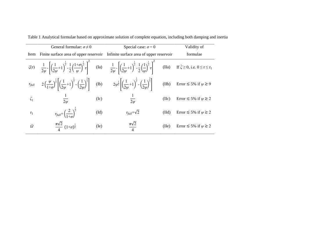
Table 1 Analytical formulae based on approximate solution of complete equation, including both damping and inertia
Item
General formulae: σ ≠ 0
Finite surface area of upper reservoir
Special case: σ = 0
Infinite surface area of upper reservoir
Validity of
formulae
ζ(τ) 1
2ψ- [(
1
2ψ+1)
12
-1
2(1+σ
ψ)
12
τ]
2
(Ia) 1
2ψ- [(
1
2ψ+1)
12
-1
2(
1
ψ)
12
τ]
2
(IIa) If ζ ≥ 0, i.e. 0 ≤ τ ≤ τ1
τfull 2 (ψ
1+σ)
12
[(1
2ψ+1)
12
- (1
2ψ)
12
] (Ib) 2ψ12 [(
1
2ψ+1)
12
- (1
2ψ)
12
] (IIb) Error ≲ 5% if ψ ≳ 9
ζ1 1
2ψ (Ic)
1
2ψ (IIc) Error ≲ 5% if ψ ≳ 2
τ1 τfull+ (2
1+σ)
12
(Id) τfull+√2 (IId) Error ≲ 5% if ψ ≳ 2
Ω π√2
4 (1+σ)
12 (Ie)
π√2
4 (IIe) Error ≲ 5% if ψ ≳ 2
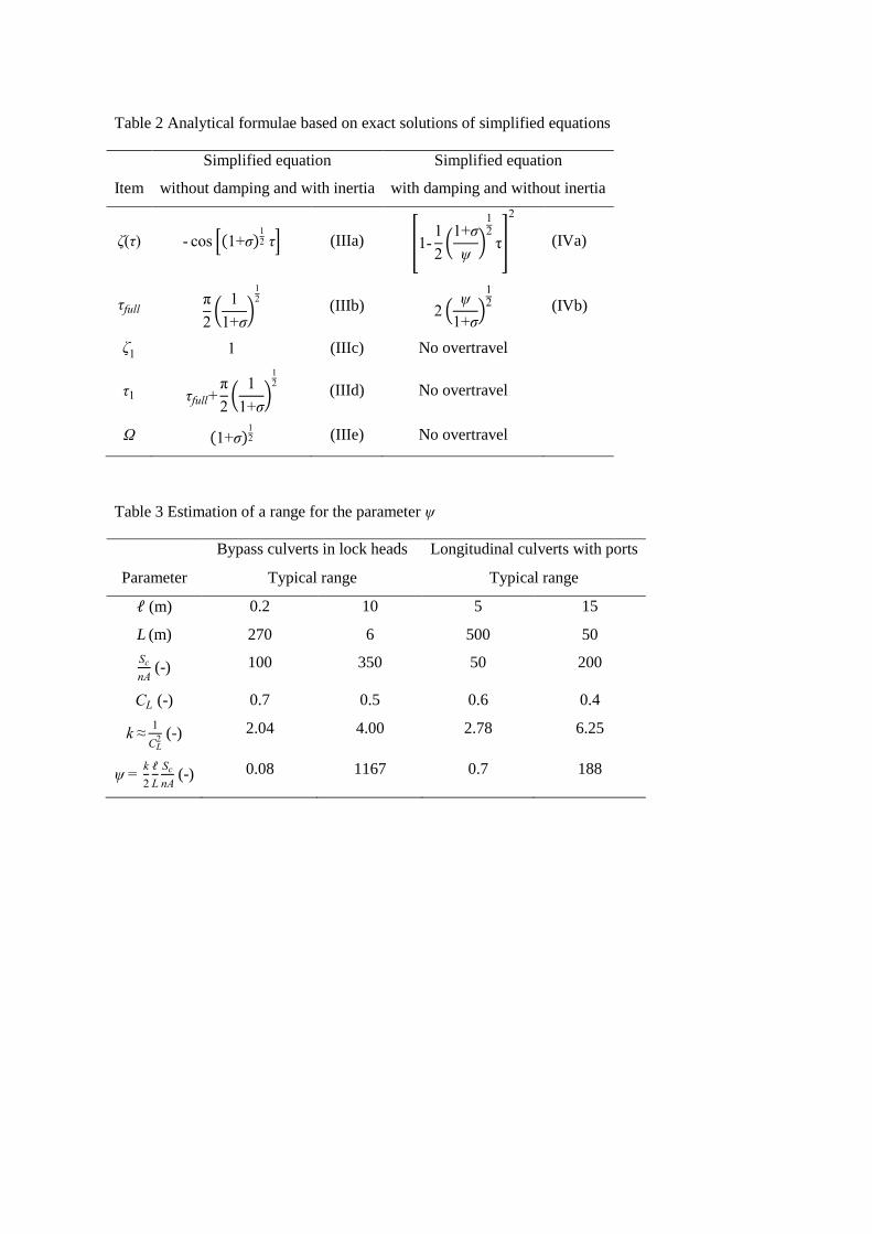
Table 2 Analytical formulae based on exact solutions of simplified equations
Item
Simplified equation
without damping and with inertia
Simplified equation
with damping and without inertia
ζ(τ) - cos [(1+σ)12 τ] (IIIa) [1-
1
2(
1+σ
ψ)
12
τ]
2
(IVa)
τfull π
2(
1
1+σ)
12
(IIIb) 2 (ψ
1+σ)
12 (IVb)
ζ1 1 (IIIc) No overtravel
τ1 τfull+π
2(
1
1+σ)
12
(IIId) No overtravel
Ω (1+σ)12 (IIIe) No overtravel
Table 3 Estimation of a range for the parameter ψ
Parameter
Bypass culverts in lock heads Longitudinal culverts with ports
Typical range Typical range
ℓ (m) 0.2 10 5 15
L (m) 270 6 500 50
Sc
nA (-) 100 350 50 200
CL (-) 0.7 0.5 0.6 0.4
k ≈1
CL2 (-) 2.04 4.00 2.78 6.25
ψ = k
2
ℓ
L
Sc
nA (-) 0.08 1167 0.7 188
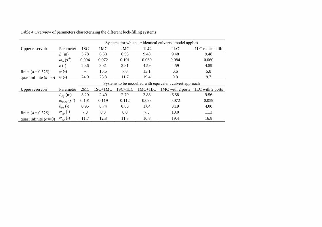
Table 4 Overview of parameters characterizing the different lock-filling systems
Systems for which “n identical culverts” model applies
Upper reservoir Parameter 1SC 1MC 2MC 1LC 2LC 1LC reduced lift
L (m) 3.78 6.58 6.58 9.48 9.48 9.48
ωo (s-1
) 0.094 0.072 0.101 0.060 0.084 0.060
k (-) 2.36 3.81 3.81 4.59 4.59 4.59
finite (σ = 0.325) ψ (-) - 15.5 7.8 13.1 6.6 5.8
quasi infinite (σ ≈ 0) ψ (-) 24.9 23.3 11.7 19.4 9.8 9.7
Systems to be modelled with equivalent culvert approach
Upper reservoir Parameter 2MC 1SC+1MC 1SC+1LC 1MC+1LC 1MC with 2 ports 1LC with 2 ports
Leq (m) 3.29 2.40 2.70 3.88 6.58 9.56
ωo,eq (s-1
) 0.101 0.119 0.112 0.093 0.072 0.059
keq (-) 0.95 0.74 0.80 1.04 3.19 4.00
finite (σ = 0.325) ψeq
(-) 7.8 8.3 8.0 7.3 13.0 11.3
quasi infinite (σ ≈ 0) ψeq
(-) 11.7 12.3 11.8 10.8 19.4 16.8

Table 5 Filling time tfull as predicted by analytical formulae (Ib), (IIb), (18) and LOCKSIM, in comparison to the value derived from the measurements
Systems for which “n identical culverts” model applies
Upper reservoir Parameter tfull 1SC 1MC 2MC 1LC 2LC 1LC reduced lift
finite (σ = 0.325) measured (s) - 84.0 40.0 90.0 42.2 59.2
predicted (Ib) (s) - 79.7 37.2 86.7 40.1 52.2
predicted (Ib)/measured (-) - 0.95 0.93 0.96 0.95 0.88
predicted (IIb)/measured (-) - 1.09 1.07 1.11 1.09 1.02
predicted (16)/measured (-) - 1.31 1.38 1.35 1.44 1.36
quasi infinite (σ ≈ 0) measured (s) 100.5 124.5 61.8 133.5 64.4 91.2
predicted (Ib or IIb) (s) 91.8 116.4 55.0 125.9 59.1 83.4
predicted (Ib or IIb)/measured (-) 0.91 0.93 0.89 0.94 0.92 0.91
predicted (16)/measured (-) 1.05 1.08 1.09 1.11 1.15 1.14
predicted (LOCKSIM1)/measured (-) 0.93 0.95 0.92 0.96 0.95 0.95
predicted (LOCKSIM2)/measured (-) 0.96 0.98 0.98 0.98 1.01 0.98
predicted (LOCKSIM3)/measured (-) 0.96 0.98 0.98 0.99 1.01 0.99
Systems to be modelled with equivalent culvert approach
Upper reservoir Parameter tfull 2MC 1SC+1MC 1SC+1LC 1MC+1LC 1MC with 2 ports 1LC with 2 ports
finite (σ = 0.325) measured (s) 40.0 35.2 36.9 41.4 77.3 85.5
predicted (Ib) (s) 37.2 33.1 34.3 38.8 72.0 79.7
predicted (Ib)/measured (-) 0.93 0.94 0.93 0.94 0.93 0.93
predicted (IIb)/measured (-) 1.07 1.08 1.07 1.08 1.07 1.08
predicted (16)/measured (-) 1.38 1.38 1.37 1.40 1.30 1.33
quasi infinite (σ ≈ 0) measured (s) 61.8 53.9 55.3 62.2 113.1 125.0
predicted (Ib or IIb) (s) 54.9 48.5 50.2 56.9 104.8 115.8
predicted (Ib or IIb)/measured (-) 0.89 0.90 0.91 0.91 0.93 0.93
predicted (16)/measured (-) 1.09 1.10 1.11 1.13 1.09 1.10
predicted (LOCKSIM1)/measured (-) 0.92 0.93 0.94 0.95 0.95 0.95
predicted (LOCKSIM2)/measured (-) 0.98 0.98 0.99 1.00 0.96 0.96
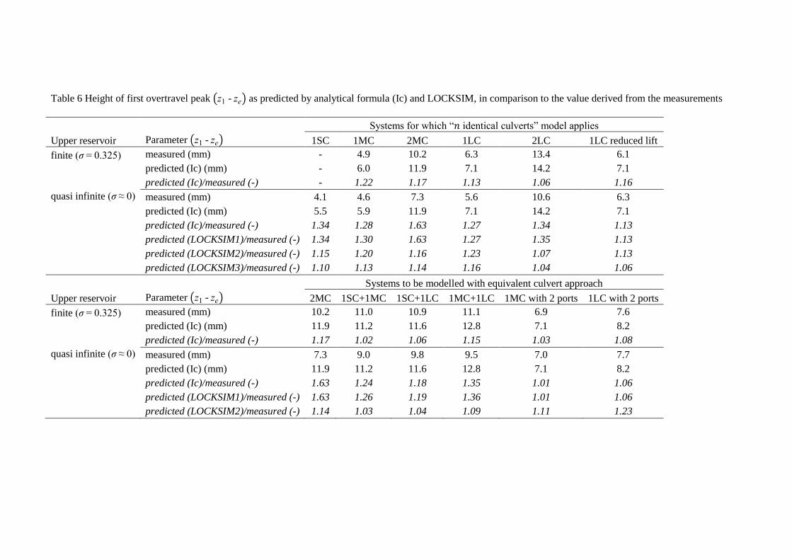
Table 6 Height of first overtravel peak (z1 - ze) as predicted by analytical formula (Ic) and LOCKSIM, in comparison to the value derived from the measurements
Systems for which “𝑛 identical culverts” model applies
Upper reservoir Parameter (z1 - ze) 1SC 1MC 2MC 1LC 2LC 1LC reduced lift
finite (σ = 0.325) measured (mm) - 4.9 10.2 6.3 13.4 6.1
predicted (Ic) (mm) - 6.0 11.9 7.1 14.2 7.1
predicted (Ic)/measured (-) - 1.22 1.17 1.13 1.06 1.16
quasi infinite (σ ≈ 0) measured (mm) 4.1 4.6 7.3 5.6 10.6 6.3
predicted (Ic) (mm) 5.5 5.9 11.9 7.1 14.2 7.1
predicted (Ic)/measured (-) 1.34 1.28 1.63 1.27 1.34 1.13
predicted (LOCKSIM1)/measured (-) 1.34 1.30 1.63 1.27 1.35 1.13
predicted (LOCKSIM2)/measured (-) 1.15 1.20 1.16 1.23 1.07 1.13
predicted (LOCKSIM3)/measured (-) 1.10 1.13 1.14 1.16 1.04 1.06
Systems to be modelled with equivalent culvert approach
Upper reservoir Parameter (z1 - ze) 2MC 1SC+1MC 1SC+1LC 1MC+1LC 1MC with 2 ports 1LC with 2 ports
finite (σ = 0.325) measured (mm) 10.2 11.0 10.9 11.1 6.9 7.6
predicted (Ic) (mm) 11.9 11.2 11.6 12.8 7.1 8.2
predicted (Ic)/measured (-) 1.17 1.02 1.06 1.15 1.03 1.08
quasi infinite (σ ≈ 0) measured (mm) 7.3 9.0 9.8 9.5 7.0 7.7
predicted (Ic) (mm) 11.9 11.2 11.6 12.8 7.1 8.2
predicted (Ic)/measured (-) 1.63 1.24 1.18 1.35 1.01 1.06
predicted (LOCKSIM1)/measured (-) 1.63 1.26 1.19 1.36 1.01 1.06
predicted (LOCKSIM2)/measured (-) 1.14 1.03 1.04 1.09 1.11 1.23

Table 7 Frequency of chamber surface oscillations around equalization level ω as predicted by analytical formula (Ie), in comparison to the value derived from the
measurements
Systems for which “𝑛 identical culverts” model applies
Upper reservoir Parameter ω 1SC 1MC 2MC 1LC 2LC 1LC reduced lift
finite (σ = 0.325) measured (s-1
) - 0.088 0.135 0.074 0.097 0.074
predicted (Ie) (s-1
) - 0.092 0.130 0.076 0.108 0.076
predicted (Ie)/measured (-) - 1.05 0.96 1.03 1.11 1.03
quasi infinite (σ ≈ 0) measured (s-1
) 0.092 0.070 0.115 0.059 0.084 0.076
predicted (Ie) (s-1
) 0.105 0.080 0.113 0.066 0.094 0.066
predicted (Ie)/measured (-) 1.14 1.14 0.98 1.12 1.12 0.87
Systems to be modelled with equivalent culvert approach
Upper reservoir Parameter ω 2MC 1SC+1MC 1SC+1LC 1MC+1LC 1MC with 2 ports 1LC with 2 ports
finite (σ = 0.325) measured (s-1
) 0.135 0.125 0.123 0.122 0.071 0.068
predicted (Ie) (s-1
) 0.130 0.152 0.143 0.119 0.092 0.076
predicted (Ie)/measured (-) 0.96 1.22 1.16 0.98 1.30 1.12
quasi infinite (σ ≈ 0) measured (s-1
) 0.115 0.110 0.116 0.096 0.064 0.057
predicted (Ie) (s-1
) 0.113 0.132 0.124 0.104 0.080 0.066
predicted (Ie)/measured (-) 0.98 1.20 1.07 1.08 1.25 1.16
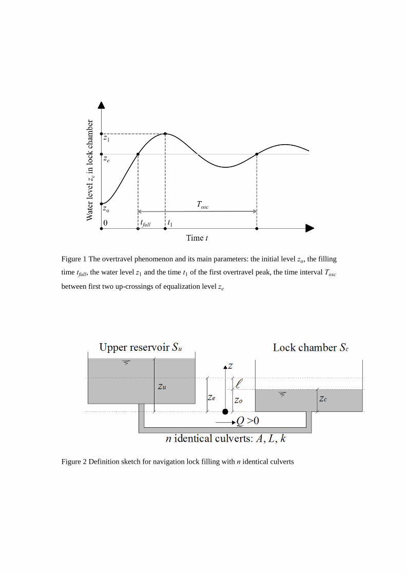
Figure 1 The overtravel phenomenon and its main parameters: the initial level zo, the filling
time tfull, the water level z1 and the time t1 of the first overtravel peak, the time interval Tosc
between first two up-crossings of equalization level ze
Figure 2 Definition sketch for navigation lock filling with n identical culverts

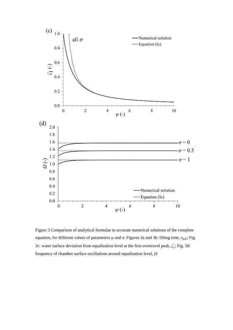
Figure 3 Comparison of analytical formulae to accurate numerical solutions of the complete
equation, for different values of parameters ψ and σ. Figures 3a and 3b: filling time, τfull; Fig.
3c: water surface deviation from equalization level at the first overtravel peak, ζ1; Fig. 3d:
frequency of chamber surface oscillations around equalization level, Ω
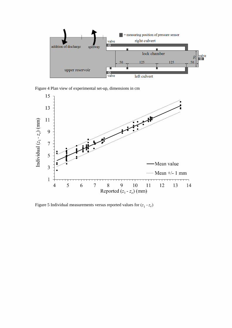
Figure 4 Plan view of experimental set-up, dimensions in cm
Figure 5 Individual measurements versus reported values for (z1 - ze)