On a Practical Methodology for Solving BVP Problems … · 1356 U. Filobello-Nino et al.: On a...

Appl. Math. Inf. Sci.10, No. 4, 1355-1367 (2016) 1355

Applied Mathematics & Information SciencesAn International Journal

http://dx.doi.org/10.18576/amis/100414

On a Practical Methodology for Solving BVP Problemsby Using a Modified Version of Picard Method

U. Filobello-Nino1, H. Vazquez-Leal1∗, A. Perez-Sesma1, J. Cervantes-Perez1, L. Hernandez-Martinez2, A. Herrera-May3,V. M. Jimenez-Fernandez1, A. Marin-Hernandez4, C. Hoyos-Reyes1, A. Diaz-Sanchez2 and J. Huerta Chua5

1 Electronic Instrumentation and Atmospheric Sciences School, Universidad Veracruzana, Cto. Gonzalo Aguirre Beltran S/N, 91000,Xalapa, Veracruz, Mexico.

2 National Institute for Astrophysics, Optics and Electronics, Luis Enrique Erro #1, Sta. Marıa Tonantzintla 72840, Puebla, Mexico.3 Micro and Nanotechnology Research Center, University of Veracruz, Calzada, Ruiz Cortines 455, Boca del Rio 94292, Veracruz,

Mexico.4 Department of Artificial Intelligence, Universidad Veracruzana Sebastian Camacho 5 Centro, 91000, Xalapa, Veracruz, Mexico.5 Civil Engineering School, Universidad Veracruzana, Venustiano Carranza S/N, Col. Revolucion, 93390, Poza Rica, Veracruz, Mexico.

Received: 27 Mar. 2016, Revised: 13 May 2016, Accepted: 14 May 2016Published online: 1 Jul. 2016

Abstract: The aim of this paper is to propose a modified version of PicardMethod, the Boundary Value Problems Picard Method(BVPP), which allows the solution of BVP problems, with few iterations. What is more, as case study, BVPP is employed to getapproximate solutions to four differential equations; twolinear and two nonlinear. Comparing figures between approximate and exactsolutions, it is shown that BVPP method can generate handy approximate solutions with the desired degree of accuracy.

Keywords: Linear Differential Equation, Nonlinear Differential Equation, Picard Method, Approximate Solutions, Boundary ValueProblems.

1 Introduction

Solving nonlinear differential equations is relevantbecause phenomena on the frontiers of modern sciencesare often nonlinear in nature. On the engineering andscience fields, physical phenomena are frequentlymodeled using nonlinear differential equations. Scientistswho work in such disciplines constantly face theproblems of solving linear and nonlinear ordinarydifferential equations, partial differential equations,andsystems of nonlinear ordinary differential equations.Recently a wide variety of methods focused to findapproximate solutions to nonlinear differential equations,as an alternative to classical methods, have been reported.Such as those based on: variational approaches [1,2,3,4],tanh method [5], exp-function [6,7], Adomian’sdecomposition method [8,9,10,11,12,13], parameterexpansion [14], homotopy perturbation method [15,16,13,17,18,19,20,21,22,23,24,25,26,27,4,28,29,30,31,32,33,34,35,36,37,38,39,40,41], homotopy analysismethod [42,43,44,45,46], homotopy asymptotic method

[47], perturbation method [48,49], modified Taylormethod [50], generalized homotopy method [51],differential transformation method [52], among manyothers. Also, a few exact solutions to nonlineardifferential equations have been reported occasionally[53].

As it is well known, boundary value problems ofordinary differential equations have many applications insciences. The case of BVP for nonlinear ODES includes,Michaelis Menten equation [54], that describes thekinetics of enzyme-catalyzed reactions, Gelfand’sdifferential equation [35,49] which governingcombustible gas dynamics (see below, this study proposesan approximate solution for this equation), Troesch’sequation [55,56,57,58,59,60], arising in the investigationof confinement of a plasma column by a radiationpressure, among many others. On the other hand, thetheory of BVP for linear ODES, is a well establishedbranch of mathematics, with many applications. Betweenproblems of interest, related to these equations, are found:The one-dimensional quantum problem, of a particle of

∗ Corresponding author e-mail:[email protected]

c© 2016 NSPNatural Sciences Publishing Cor.

http://dx.doi.org/10.18576/amis/100414

1356 U. Filobello-Nino et al.: On a practical methodology for solving BVP problems...

mass m confined in a region of zero potential by aninfinite potential at two points x=a and x=b [61], Heattransfer equation [61], Wave equation which describes forinstance, transverse vibrations of a uniform stretchedstring between two fixed points, let us say x = a and x = b[62], The Laplace equation, which governs thetemperature field corresponding to the steady state in aplate [62], and so on. Generally, many problemsexpressed in terms of partial differential equations, giverise through method of separation of variables, to BVP forlinear ODES [61,62].

The Picard Iteration Method (PIM) [63,64,65] is awell established iterative method; although it has beenemployed above all as a formal procedure for establishingthe existence and uniqueness theorems of differentialequations, their usefulness in practice is relatively small.This is mainly due to the convergence of the method isslow, and also because the integration process involved,rapidly becomes very long and tedious. Nevertheless, thetechnique has several significant advantages. Unlike otherknown methods, Picard’s method applies to linear andnonlinear problems, with identical ease. Also, based onwell-established criteria and theorems, PIM allows topredict from the beginning, if the iterative processinvolved will converge to the solution of the problem,even if such solution is unique, which many methods fornonlinear differential equations cannot guarantee.

Our main goal in this study is take advantage of thefortress of the method, and try to solve its drawbacks,with the end to employ it, as a useful tool to obtainapproximate solutions of BVP problems for linear andnonlinear ordinary second order differential equations.This paper is organized as follows. In Section2, a briefreview of the basic idea for Picard iteration method isprovided. In Section3, we will present, the BoundaryValue Problems Picard Method (BVPP) as a modifiedversion of Picard method. Additionally, Section4presents four cases study, including a comparison ofBVPP with other methods to show its precision andversatility. Besides a discussion on the results is presentedin Section 5. Finally, a brief conclusion is given inSection .6

2 Picard Iteration Method.

We begin reformulating the initial value problem

y′′ (t) = f (t,y(t),y′(t)); y(t0) = A, y′(t0) = B(1)

as the following equivalent integral equation

y(t) = A+Bt+∫ t

t0

∫ t

t0f(

t ′,y(t ′),y′(t ′))

dt′dt, (2)

The solution for (2) can be expressed as the limit of asequence of functionsyn (t), in the limit n → ∞, inaccordance with the recurrence formula

yn(t) = A+Bt+∫ t

t0

∫ t

t0f(

t ′,yn−1(t′),y′n−1(t

′))

dt′dt,

n= 1,2,3..(3)

When the right hand side of (1), f (t,y(t),y′(t)) is acontinuous function for all its arguments, and havingcontinuous first partial derivatives with respect toy andy′

in a neighborhood of the initial conditions of (1) then, it iswell known that regardless of the choice of the initialfunction y0(t), the sequence{yn(t)}, generated by theiterative process given by (3), converges to a solution ofthe problem (1) [62,66,67,68].

In the same way, assuming thatf (t,y(t),y′(t)) satisfiesthe Lipschitz condition, it would be possible to establish,amore strong but usually difficult to apply criterion. For thepurposes of this study, it is sufficient to ensure that startingof the iterative process (3), we will get a solution for (2)[66,67].

3 Basic Idea of Boundary Value ProblemsPicard Method (BVPP).

Next, we will find highly accurate approximate solutionsfor boundary value problems, following a method, whichincorporates the boundary values of the original problem,to the classical version of Picard method with initialconditions.

An important case of BVP problems, is one where thevalues of the sought solution are given at two pointst0 andt1, but not the derivatives (Dirichlet boundary conditions),i.e.

y′′ (t) = f (t,y(t),y′(t)); y(t0) = A, y(t1) =C,(4)

therefore the value for the derivative att0, will be denotedby y′(t0) = β . We will approach our BVP problem,assuming for the time being, that the value ofβ is known(although it is initially unknown) and right hand side of(4) is a continuous function. Besides, we will use thefreedom to choose the trial functiony0(t), in order toinclude both boundary values and accelerate theconvergence of the method. Thus, we exploit the virtuesof PIM, remedying its defects.

It should be noted that, the unknown value ofy′(t0),will be determined, as part of the proposed procedure.

The method begins proposing as trial function apolynomial functionP(t) which contains one or moreparametersD,E,F, .. to be determined.

y0(t) = P(t,D,E,F, ..). (5)


Appl. Math. Inf. Sci.10, No. 4, 1355-1367 (2016) /www.naturalspublishing.com/Journals.asp 1357

According to the above, BVPP method employ insteadof (2), the following integral equation

y(t) = A+β t+∫ t

t0

∫ t

t0f(

t ′,y(t ′),y′(t ′))

dt′dt, (6)

where, the value ofβ is unknown for the time being .The solution for (6) can be expressed as the limit of a

sequence of functionsyn(t), in the limit n → ∞, inaccordance with the recurrence formula

yn(t,β ,D,E,F, ..) = A+β t

+

∫ t

t0

∫ t

t0f(

t ′,yn−1(t′,D,E,F, ..),y′n−1(t

′,D,E,F, ..)

)

dt′dt,

n= 1,2,3.. (7)

Since it has been assumed the continuity off (t ′,y(t ′),y′(t ′)) then, irrespective of (5), the successiveapproximations{yn(t)} (7), converge to the solution ofthe following problem, resembling (4) (see section 2).

y′′ (t) = f(

t,y(t),y′(t))

; y(t0) = A, y′(t0) = β .(8)

Next, in order to ensure that the n-th iteration ofBVPP (7), is also an approximate solution for (4), thevalues of β ,D,E,F, .., are chosen to ensure thatapproximate solutions satisfyy(t1) = C also, andtherefore (4). It will be seen that although (4) and (8) arerelated in this way in order to motivate BVPPconvergence, in practice is not required to considerexplicitly the auxiliary problem (8). Finally we indicatethree ways to calculate optimally the values of the aboveparameters, in order to accelerate the convergence andobtain highly accurate approximate solutions.

Method 1.Assuming that the nth approximation is sufficient, then

from (7) we can write symbolically

yn = H(t,β ,D,E,F, ..), (9)

where H(t,β ,D,E,F, ..), is a certain function obtainedfrom the iterative process above mentioned.

This method assume known the numerical solution of(4), so that (9) is evaluated as many points within theinterval [t0, t1] as parameters to be determined, that is tosay

yn(t0) = H(t0,β ,D,E,F, ..),

yn(t1) = H(t1,β ,D,E,F, ..),

yn(t2) = H(t2,β ,D,E,F, ..),

yn(t3) = H(t3,β ,D,E,F, ..),

yn(t4) = H(t4,β ,D,E,F, ..),

(10)

.... and so on,

where t2, t3, t4 ∈ (t0, t1) and the values ofyn(t0),yn(t1),yn(t2),yn(t3),yn(t4), .., are known.

(10) is a system of algebraic equations, whosesolution allows to determine the value of the parametersβ ,D,E,F, ..

It′

is expected that it result in a good fit, consideringseveral inner points, even the first iteration of BVPP canbe highly accurate and sufficient (see cases study).

Method 2.This proposal follows again the steps that led to (9), but

unlike the previous method, we will use a software like theNonlinear Fit built-in command from Maple 15, to identifyoptimally the parametersβ ,D,E,F, ..

Method 3.This method aims to determine the above parameters,

by using the least squares method.To get that (9) corresponds to a good approximate

analytic solution of (4), we have to optimize the values ofβ ,D,E,F, .. For it, after substituting (9) into (4), resultsthe following residual.

R(t,β ,D,E,F, ..) = y′′ (t,β ,D,E,F)

− f(

t,y(t,β ,D,E,F),y′(t,β ,D,E,F))

,(11)

Next, it is applied the least square method, minimizingthe square residual error [47]

I(β ,D,E,F, ..) =∫ t1

t0R2(t,β ,D,E,F, ..)dt, (12)

identifying the values ofβ ,D,E,F, .. from the conditions

∂ I∂β

= 0,∂ I∂D

= 0,∂ I∂E

= 0,∂ I∂F

= 0, .. (13)

Note that unlike the previous methods, the procedureoutlined by equations (11)-(13) does not require inadvance the knowledge of the numerical solution.

Once BVPP method optimize the values ofβ ,D,E,F, .. we will obtain good approximationsrequiring only a few iterations. It is expected that bychoosing other values for these parameters, it wouldgenerate an iterative process slower and cumbersome.

4 Cases Study.

In what follows, we will assume equations satisfying thecontinuity requirements mentioned.

Example 1.We will employ method 1, in order to find an

approximate Solution of Gelfand’s Equation.As it is known, Gelfand’s equation [35,49] models the

chaotic dynamics in combustible gas thermal ignition.Therefore it is important to search for accurate solutionsfor this equation.


www.naturalspublishing.com/Journals.asp


The equation to solve is

d2y(x)dx2 + εey(x) = 0,

0≤ x≤ 1, y(0) = 0, y(1) = 0, (14)

whereε is a positive parameter.It is possible to find a handy approximate solution for

(14) by applying the BVPP method.Thus, first we expand the exponential term of

Gelfand’s problem, resulting

y′′+ ε(

1+ y+12

y2+16

y3+ ..

)

= 0,

0≤ x≤ 1, y(0) = 0, y(1) = 0, (15)

Equation (6) for this case is given by

y(x) = βx− ε∫ x

0

∫ x

0

(

1+ y+12

y2)

dx′dx, (16)

after keeping the second power ofy variable.We choose as trial functiony0(x)

y0(x) = Bx+Cx2+Dx3. (17)

The corresponding recurrence formula is given by

yn(x,β ,B,C,D) = βx

− ε∫ x

0

∫ x

0

(

1+ yn−1(x,β ,B,C,D)+

+12

y2n−1(x,β ,B,C,D)

)

dx′dx.

n= 1,2,3.. (18)

The first iteration of BVPP (n=1),

y1(x,β ,B,C,D) = βx

− ε∫ x

0

∫ x

0

(

1+ y0(x,β ,B,C,D)+

+12

y20(x,β ,B,C,D)

)

dx′dx. (19)

Assuming that first iteration is sufficient, aftersubstituting (17) into (19), we obtain

y1(x,β ,B,C,D) = βx− ε2x2− εB

6 x3

+[

− εC12 +

B24

]

x4+[

D20+

BC20

]

x5

+[

C2

60 +BD30

]

x6+ CD42 x7+ D2

112x8.

(20)

In accordance with first method, we generate fouralgebraic equations, by substituting the boundary value ofx= 1, also the values:x= 0.1,x= 0.5, andx= 0.7, whichbelong to[0,1], in order to calculateβ ,B,C,D. Note thatin this case, the conditiony1(0,β ,B,C,D) = 0, isautomatically satisfied.

In order to test the effectiveness of the method, we willconsider the values ofε = 3 andε = 3.5, despite of thesolutions corresponding to values of the parameterε ≥ 1,are considered the most difficult to model [47,69,70].

The solution for the described system of algebraicequations forε = 3, results in

β = 2.321014274, B= 2.725506295,

C=−0.9993962770, D = 2.181675403.

By substituting these values into (20) is obtained thefollowing approximate solution for (14).

y1(x) = 2.321014274x−1.5x2−1.362753148x3

+0.3634118315x4−0.027109272x5

+0.2148522168x6−0.05191329226x7

+0.04249738896x8. (21)

In the same way, the parameters forε = 3.5, are givenby

β = 3.707678793, B= 4.533738715,

C= 2.030713696, D = 2.093200793,

and the corresponding approximate solution for (14).

y1(x) = 3.707678793x−1.75x2−2.644680917x3

−0.4033857148x4+0.5649963048x5

+0.385064151x6+0.1012069409x7

+0.03912044250x8. (22)

Example 2.This example shows the use of method 2. As a case

study we propose the following nonlinear differentialequation [61].

d2y(x)dx2 − εy2(x) = 0,

0≤ x≤ 1, y(0) = 0, y(1) = 1, (23)

whereε, is a positive parameter.Equation (6) for this case is given by

y(x) = βx+ ε∫ x

0

∫ x

0y2dx′dx, (24)



next, we select as trial functiony0(x)

y0(x) = Bx+Cx2. (25)

The recurrence formula for this case is given by

yn(x,β ,B,C) = βx

+ ε∫ x

0

∫ x

0

(

y2n−1(x,β ,B,C)

)

dx′dx.

n= 1,2,3.. (26)

The first iteration of BVPP results in

y1(x,β ,B,C) = βx+ε∫ x

0

∫ x

0

(

y20(x,β ,B,C)

)

dx′dx. (27)

By substituting (25) into (27), we obtain

y1(x,β ,B,C) = βx+ ε[

B2x2

2+

BCx3

3+

C2x4

12

]

, (28)

from the conditiony1(1) = 1, we obtain the value

β = 1− ε[

B2

2+

BC3

+C2

12

]

, (29)

therefore

y1(x,B,C) = x+εB2

2

[

x2− x]

+εBC

3

[

x3− x]

+εC2

12

[

x4− x]

. (30)

In order to show the effectiveness of the method, weconsider as case study, a large value of the parameterε = 30. As it is well known, the solutions correspondingto values of the parameterε ≥ 1, are considered the mostdifficult to model, for equations depending on a parameteras (23) (for instance, classical perturbation method(CPM), provides in general, better results for smallperturbation parametersε << 1, see below) [47,69,70].

Thus, (30) adopts the form

y1(x,B,C) = x+15B2[x2− x]

+10BC[

x3− x]

+5C2

2

[

x4− x]

. (31)

To get that (31) corresponds to an accurate analyticalapproximate solution of (23), we identify optimally theconstantsC and B by using the Nonlinear Fit built-incommand from Maple 15, which results in

B = −0.30848851834098, andC = 1.00432567368877(from (29) β = 0.1490767537).

Substituting these values into (31), we get

y1(x) = 0.149076753781481x+1.42747748922320x2

−3.09822939008034x3+2.52167514707567x4. (32)

In order to show the accuracy of BVPP, we willcompare our approximation (32) with the following thirdorder approximate solution for (23) deduced, employingCPM

y(x) = 6.6845238095238x+13.065476190476x4

−23.214285714286x7+4.462857142857x10 (33)

(see discussion and Figure3).Example 3.This example shows the use of method 3. As a case

study we propose the following linear differential equation[62].

d2y(x)dx2 − x2y(x) = 0,

0≤ x≤ 1, y(0) = 0, y(1) = 1, (34)


y(x) = βx+∫ x

0

∫ x

0x2ydx′dx, (35)


y0(x) = B+Cx. (36)


yn(x,β ,B,C) = βx+∫ x

0

∫ x

0

(

x2yn−1(x,β ,B,C))

dx′dx.

n= 1,2,3.. (37)


y1(x,β ,B,C) = βx+∫ x

0

∫ x

0

(

x2y0(x,β ,B,C))

dx′dx.

(38)By substituting (36) into (38), we obtain

y1(x,β ,B,C) = βx+Bx4

12+

Cx5

20. (39)

Next, in order to obtain a better approximate solution,it is obtained the second iteration.




Evaluating (37), for n = 2, it is obtained

y2(x,β ,B,C) = βx+∫ x

0

∫ x

0

(

x2y1(x,β ,B,C))

dx′dx,

(40)Substituting (39) into (40), we get

y2(x,B,β ) = x9+β[

x− x9]

+β20

[

x5− x9]

+B

672

[

x8− x9], (41)

where, we employed the value

C= 1440

(

1−2120

β −B

672

)

, (42)

obtained from conditiony2(1) = 1.From the steps outlined by equations (11) - (13), we get

the following algebraic system for the unknown quantitiesβ andB.

2596941311453636800

β +3642882473

75558877954560B=

24716233145363680

,

122321146163875

β +2596941311453636800

B=776123210925

.

(43)

Thus, the values ofβ and B, which minimize thesquare residual error, are given byβ = 0.9517485996 andB=−0.01705817486.

Finally, substituting these values into (41), we get

y2(x) = 0.0006893544x9−0.00002538418878x8

+0.04758742998x5+0.9517485996x. (44)

Example 4.This case study, shows the comparison among method

2, method 3, and variation of parameters for lineardifferential equations [61,62].

We will find an approximate solution for thedifferential equation.

d2y(x)dx2 + y(x) = x10

,

0≤ x≤ 1, y(0) = 0, y(1) = 0, (45)

This equation has an exact solution as follows, usingthe method of variation of parameters (VP) for lineardifferential equations.

y(x) = Asinx+∫ x

0s10sin(x− s)ds, (46)

whereA=− 1sin1

∫ 10 s10sin(x− s)ds.

A disadvantage of VP is the big effort that must bedone to solve the integrals in (46) (each requires 10integrations by parts, in this case). Instead, we will seethat BVPP provides a solution very accurate and handyfor applications.


y(x) = βx+∫ x

0

∫ x

0(x10− y)dx′dx, (47)


y0(x) = B+Cx. (48)


yn(x,β ,B,C) = βx

+

∫ x

0

∫ x

0

(

x10− yn−1(x,β ,B,C))

dx′dx.

n= 1,2,3.. (49)


y1(x,β ,B,C) = βx+∫ x

0

∫ x

0

(

x10− y0(x,β ,B,C))

dx′dx.

(50)Substituting (48) into (50), we get

y1(x,B,C) =1

132

[

x12− x]

+B2

[

x− x2]+C6

[

x− x3].

(51)where, we used the conditiony1(1) = 0, to obtain

β =−1

132+

B2+

C6. (52)

Next, we will get two approximate solutions for (45)by using aforementioned method 2 and method 3.

Method 2To get that (51) corresponds to a precise approximate

analytic solution for (45), we identify optimally theconstantsBandC by using the Nonlinear Fit built-incommand from Maple 15, which results inB = −0.00085048287500623, andC = −0.0062854559150948 (from (52)β =−0.009048575).


y1(x) = 0.03125x12

−0.00904857499910982x+0.000425241437503110x2

+0.00104757598584913x3 (53)



Method 3In this case, we will identify the constantsB andC

following the steps outlined by equations (11) - (13), sothat

110189

C+101120

B=−221

60480,

101120

C+10160

B=−127

21840.

(54)

By solving the above algebraic system, we find thatthe values ofB and C, minimizing the square residualerror, are given byB = −0.0011384093831064 andC=−0.0046321138852940.


y1(x) = 0.03125x12

−0.0089169812481931x+0.00056920469155320x2

+0.00077201898088233x3, (55)

from (52) results the valueβ =−0.008916981249.

5 Discussion

This paper proposed a modified version of PicardMethod, the Boundary Value Problems Picard Method(BVPP), in order to find approximate solutions for BVPproblems. One of the main results, which follows fromthe accuracy of the approximate results obtained byBVPP, is that the slow convergence of PIM, isconsequence of a inadequate choice of the trial function(even, many authors suggest starting Picard iterativeprocess, by using as trial function, the initial condition ofthe differential equation to solve). The procedurefollowed by BVPP relies on the auxiliary initial valueproblem (8), where the value ofy′(t0) = β , is unknown.Assuming that the right hand sidef (t,y(t),y′(t)) and itspartial derivatives; satisfy certain continuity conditions(as it was explained) then irrespective of trial function,the successive approximations{yn(t)} (7) converge to thesolution of (8).

In order to get that{yn(t)} also become in a solutionfor (4), we employed in our examples, as trial functions,some polynomial functions of different degreescontaining some parameters, which were determined sothat, the approximate solution, satisfies both boundaryconditions of (4) and also contributed to improve theprocess of getting adequate trial functions. With thispurpose, we proposed three methods to calculateoptimally the mentioned parameters. As a matter of fact,we obtained highly accurate analytical approximatesolutions.

The first method assumes as known the numericalsolution for (4), so that the approximate solution given bythe BVPP method, is evaluated at many points within theinterval of interest as parameters to be determined. Theabove procedure gives rise to a system of algebraicequations, whose solution let determines the value of theparameters.

The second method proposed a software like theNonlinear Fit built-in command from Maple 15, toidentify optimally the constants.

The third method determines the adjusting parameters,by using the least squares method.

Next, we applied BVPP method to find approximatesolutions to four differential equations, from which twowere nonlinear and the others linear.

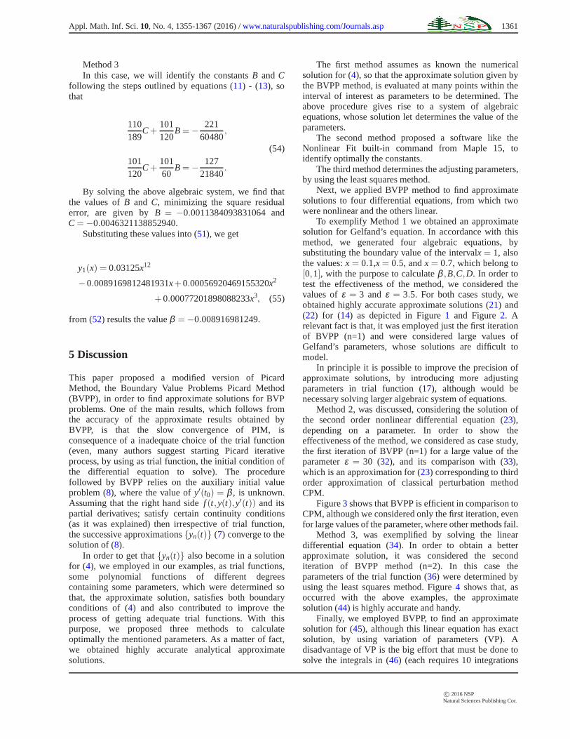
To exemplify Method 1 we obtained an approximatesolution for Gelfand’s equation. In accordance with thismethod, we generated four algebraic equations, bysubstituting the boundary value of the intervalx= 1, alsothe values:x = 0.1,x= 0.5, andx = 0.7, which belong to[0,1], with the purpose to calculateβ ,B,C,D. In order totest the effectiveness of the method, we considered thevalues ofε = 3 and ε = 3.5. For both cases study, weobtained highly accurate approximate solutions (21) and(22) for (14) as depicted in Figure1 and Figure2. Arelevant fact is that, it was employed just the first iterationof BVPP (n=1) and were considered large values ofGelfand’s parameters, whose solutions are difficult tomodel.

In principle it is possible to improve the precision ofapproximate solutions, by introducing more adjustingparameters in trial function (17), although would benecessary solving larger algebraic system of equations.

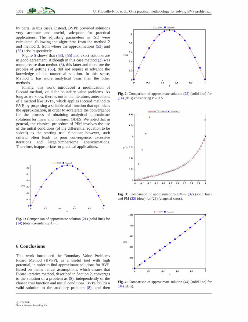
Method 2, was discussed, considering the solution ofthe second order nonlinear differential equation (23),depending on a parameter. In order to show theeffectiveness of the method, we considered as case study,the first iteration of BVPP (n=1) for a large value of theparameterε = 30 (32), and its comparison with (33),which is an approximation for (23) corresponding to thirdorder approximation of classical perturbation methodCPM.

Figure3 shows that BVPP is efficient in comparison toCPM, although we considered only the first iteration, evenfor large values of the parameter, where other methods fail.

Method 3, was exemplified by solving the lineardifferential equation (34). In order to obtain a betterapproximate solution, it was considered the seconditeration of BVPP method (n=2). In this case theparameters of the trial function (36) were determined byusing the least squares method. Figure4 shows that, asoccurred with the above examples, the approximatesolution (44) is highly accurate and handy.

Finally, we employed BVPP, to find an approximatesolution for (45), although this linear equation has exactsolution, by using variation of parameters (VP). Adisadvantage of VP is the big effort that must be done tosolve the integrals in (46) (each requires 10 integrations




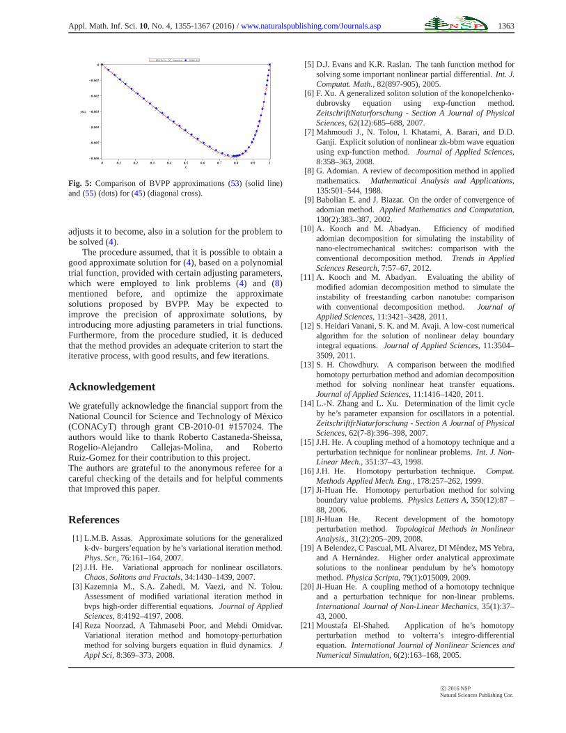
by parts, in this case). Instead, BVPP provided solutionsvery accurate and useful, adequate for practicalapplications. The adjusting parameters in (51) werecalculated, following the algorithms from the method 2and method 3, from where the approximations (53) and(55) arise respectively.

Figure5 shows that (53), (55) and exact solution arein good agreement. Although in this case method (2) wasmore precise than method (3), this latter and therefore theprocess of getting (55), did not require in advance theknowledge of the numerical solution. In this sense,Method 3 has more analytical basis than the othermethods.

Finally, this work introduced a modification ofPiccard method, valid for boundary value problems. Aslong as we know, there is not in the literature, antecedentsof a method like BVPP, which applies Piccard method toBVP, by proposing a suitable trial function that optimizesthe approximation, in order to accelerate the convergencefor the process of obtaining analytical approximatesolutions for linear and nonlinear ODES. We noted that ingeneral, the classical procedure of PIM involves the useof the initial conditions (of the differential equation to besolved) as the starting trial function; however, suchcriteria often leads to poor convergence, excessiveiterations and large/cumbersome approximations.Therefore, inappropriate for practical applications.

Fig. 1: Comparison of approximate solution (21) (solid line) for(14) (dots) consideringε = 3

6 Conclusions

This work introduced the Boundary Value ProblemsPicard Method (BVPP), as a useful tool with highpotential, in order to find approximate solutions for BVP.Based on mathematical assumptions, which ensure thatPicard iterative method, described in Section 2, convergesto the solution of a problem as (8), independently of thechosen trial function and initial conditions. BVPP builds avalid solution to the auxiliary problem (8), and then

Fig. 2: Comparison of approximate solution (22) (solid line) for(14) (dots) consideringε = 3.5

Fig. 3: Comparison of approximations BVPP (32) (solid line)and PM (33) (dots) for (23) (diagonal cross).

Fig. 4: Comparison of approximate solution (44) (solid line) for(34) (dots).



Fig. 5: Comparison of BVPP approximations (53) (solid line)and (55) (dots) for (45) (diagonal cross).

adjusts it to become, also in a solution for the problem tobe solved (4).

The procedure assumed, that it is possible to obtain agood approximate solution for (4), based on a polynomialtrial function, provided with certain adjusting parameters,which were employed to link problems (4) and (8)mentioned before, and optimize the approximatesolutions proposed by BVPP. May be expected toimprove the precision of approximate solutions, byintroducing more adjusting parameters in trial functions.Furthermore, from the procedure studied, it is deducedthat the method provides an adequate criterion to start theiterative process, with good results, and few iterations.

Acknowledgement

We gratefully acknowledge the financial support from theNational Council for Science and Technology of Mexico(CONACyT) through grant CB-2010-01 #157024. Theauthors would like to thank Roberto Castaneda-Sheissa,Rogelio-Alejandro Callejas-Molina, and RobertoRuiz-Gomez for their contribution to this project.The authors are grateful to the anonymous referee for acareful checking of the details and for helpful commentsthat improved this paper.

References

[1] L.M.B. Assas. Approximate solutions for the generalizedk-dv- burgers’equation by he’s variational iteration method.Phys. Scr., 76:161–164, 2007.

[2] J.H. He. Variational approach for nonlinear oscillators.Chaos, Solitons and Fractals, 34:1430–1439, 2007.

[3] Kazemnia M., S.A. Zahedi, M. Vaezi, and N. Tolou.Assessment of modified variational iteration method inbvps high-order differential equations.Journal of AppliedSciences, 8:4192–4197, 2008.

[4] Reza Noorzad, A Tahmasebi Poor, and Mehdi Omidvar.Variational iteration method and homotopy-perturbationmethod for solving burgers equation in fluid dynamics.JAppl Sci, 8:369–373, 2008.

[5] D.J. Evans and K.R. Raslan. The tanh function method forsolving some important nonlinear partial differential.Int. J.Computat. Math., 82(897-905), 2005.

[6] F. Xu. A generalized soliton solution of the konopelchenko-dubrovsky equation using exp-function method.ZeitschriftNaturforschung - Section A Journal of PhysicalSciences, 62(12):685–688, 2007.

[7] Mahmoudi J., N. Tolou, I. Khatami, A. Barari, and D.D.Ganji. Explicit solution of nonlinear zk-bbm wave equationusing exp-function method.Journal of Applied Sciences,8:358–363, 2008.

[8] G. Adomian. A review of decomposition method in appliedmathematics. Mathematical Analysis and Applications,135:501–544, 1988.

[9] Babolian E. and J. Biazar. On the order of convergence ofadomian method.Applied Mathematics and Computation,130(2):383–387, 2002.

[10] A. Kooch and M. Abadyan. Efficiency of modifiedadomian decomposition for simulating the instability ofnano-electromechanical switches: comparison with theconventional decomposition method.Trends in AppliedSciences Research, 7:57–67, 2012.

[11] A. Kooch and M. Abadyan. Evaluating the ability ofmodified adomian decomposition method to simulate theinstability of freestanding carbon nanotube: comparisonwith conventional decomposition method. Journal ofApplied Sciences, 11:3421–3428, 2011.

[12] S. Heidari Vanani, S. K. and M. Avaji. A low-cost numericalalgorithm for the solution of nonlinear delay boundaryintegral equations.Journal of Applied Sciences, 11:3504–3509, 2011.

[13] S. H. Chowdhury. A comparison between the modifiedhomotopy perturbation method and adomian decompositionmethod for solving nonlinear heat transfer equations.Journal of Applied Sciences, 11:1416–1420, 2011.

[14] L.-N. Zhang and L. Xu. Determination of the limit cycleby he’s parameter expansion for oscillators in a potential.ZeitschriftfrNaturforschung - Section A Journal of PhysicalSciences, 62(7-8):396–398, 2007.

[15] J.H. He. A coupling method of a homotopy technique and aperturbation technique for nonlinear problems.Int. J. Non-Linear Mech., 351:37–43, 1998.

[16] J.H. He. Homotopy perturbation technique.Comput.Methods Applied Mech. Eng., 178:257–262, 1999.

[17] Ji-Huan He. Homotopy perturbation method for solvingboundary value problems.Physics Letters A, 350(12):87 –88, 2006.

[18] Ji-Huan He. Recent development of the homotopyperturbation method. Topological Methods in NonlinearAnalysis,, 31(2):205–209, 2008.

[19] A Belendez, C Pascual, ML Alvarez, DI Mendez, MS Yebra,and A Hernandez. Higher order analytical approximatesolutions to the nonlinear pendulum by he’s homotopymethod.Physica Scripta, 79(1):015009, 2009.

[20] Ji-Huan He. A coupling method of a homotopy techniqueand a perturbation technique for non-linear problems.International Journal of Non-Linear Mechanics, 35(1):37–43, 2000.

[21] Moustafa El-Shahed. Application of he’s homotopyperturbation method to volterra’s integro-differentialequation. International Journal of Nonlinear Sciences andNumerical Simulation, 6(2):163–168, 2005.




[22] Ji-Huan He. Some asymptotic methods for stronglynonlinear equations. International Journal of ModernPhysics B, 20(10):1141–1199, 2006.

[23] DD Ganji, H Babazadeh, F Noori, MM Pirouz, andM Janipour. An application of homotopy perturbationmethod for non linear blasius equation to boundary layerflow over a flat plate. International Journal of NonlinearScience, 7(4):399–404, 2009.

[24] DD Ganji, H Mirgolbabaei, Me Miansari, and Mo Miansari.Application of homotopy perturbation method to solvelinear and non-linear systems of ordinary differentialequations and differential equation of order three.Journalof Applied Sciences, 8:1256–1261, 2008.

[25] A Fereidoon, Y Rostamiyan, M Akbarzade, andDavood Domiri Ganji. Application of hes homotopyperturbation method to nonlinear shock damper dynamics.Archive of Applied Mechanics, 80(6):641–649, 2010.

[26] P.R. Sharma and Giriraj Methi. Applications of homotopyperturbation method to partial differential equations.AsianJournal of Mathematics & Statistics, 4:140–150, 2011.

[27] Hossein Aminikhah. Analytical approximation to thesolution of nonlinear blasius viscous flow equation byltnhpm. ISRN Mathematical Analysis, 2012, 2012.

[28] Hector Vazquez-Leal, Uriel Filobello-Nino, RobertoCastaneda-Sheissa, Luis Hernandez-Martınez, andArturo Sarmiento-Reyes. Modified hpms inspired byhomotopy continuation methods.Mathematical Problemsin Engineering, 2012, 2012.

[29] Hector Vazquez-Leal, Roberto Castaneda-Sheissa, UrielFilobello-Nino, Arturo Sarmiento-Reyes, and JesusSanchez Orea. High accurate simple approximation ofnormal distribution integral. Mathematical problems inengineering, 2012, 2012.

[30] U Filobello-Nino, Hector Vazquez-Leal, R Castaneda-Sheissa, A Yildirim, L Hernandez-Martinez, D Pereyra-Diaz, A Perez-Sesma, and C Hoyos-Reyes. An approximatesolution of blasius equation by using hpm method.AsianJournal of Mathematics & Statistics, 5(2):50, 2012.

[31] Jafar Biazar and Hossein Aminikhah. Study of convergenceof homotopy perturbation method for systems of partialdifferential equations. Computers & Mathematics withApplications, 58(11):2221–2230, 2009.

[32] Jafar Biazar and Hosein Ghazvini. Convergence ofthe homotopy perturbation method for partial differentialequations. Nonlinear Analysis: Real World Applications,10(5):2633–2640, 2009.

[33] U Filobello-Nino, H Vazquez-Leal, Y Khan, R Castaneda-Sheissa, A Yildirim, L Hernandez-Martinez, J Sanchez-Orea, R Castaneda-Sheissa, and F Rabago Bernal. Hpmapplied to solve nonlinear circuits: a study case.Appl MathSci, 6(85-88):4331–4344, 2012.

[34] DD Ganji, AR Sahouli, and M Famouri. A new modificationof hes homotopy perturbation method for rapid convergenceof nonlinear undamped oscillators.Journal of AppliedMathematics and Computing, 30(1-2):181–192, 2009.

[35] U Filobello-Nino, H Vazquez-Leal, Y Khan, A Perez-Sesma, A Diaz-Sanchez, VM Jimenez-Fernandez,A Herrera-May, D Pereyra-Diaz, JM Mendez-Perez, andJ Sanchez-Orea. Laplace transform-homotopy perturbationmethod as a powerful tool to solve nonlinear problemswith boundary conditions defined on finite intervals.

Computational and Applied Mathematics, 34(1):1–16,2013.

[36] MA Fariborzi Araghi and B Rezapour. Application ofhomotopy perturbation method to solve multidimensionalschrodinger’s equations. International Journal ofMathematical Archive (IJMA) ISSN 2229-5046, 2(11):1–6,2011.

[37] MF Araghi and M Sotoodeh. An enhanced modifiedhomotopy perturbation method for solving nonlinearvolterra and fredholm integro-differential equation.WorldApplied Sciences Journal, 20(12):1646–1655, 2012.

[38] Mahdi Bayat, Mahmoud Bayat, and Iman Pakar. Nonlinearvibration of an electrostatically actuated microbeam.LatinAmerican Journal of Solids and Structures, 11(3):534–544,2014.

[39] M Bayat, I Pakar, and A Emadi. Vibration ofelectrostatically actuated microbeam by means ofhomotopy perturbation method.Structural Engineering andMechanics, 48(6):823–831, 2013.

[40] Jafar Biazar and Behzad Ghanbari. The homotopyperturbation method for solving neutral functional–differential equations with proportional delays.Journal ofKing Saud University-Science, 24(1):33–37, 2012.

[41] Jafar Biazar and Mostafa Eslami. A new homotopyperturbation method for solving systems of partialdifferential equations. Computers & Mathematics withApplications, 62(1):225–234, 2011.

[42] Twinkle Patel, MN Mehta, and VH Pradhan. The numericalsolution of burgers equation arising into the irradiation oftumour tissue in biological diffusing system by homotopyanalysis method.Asian J Appl Sci, 5:60–66, 2012.

[43] A Basiri Parsa, MM Rashidi, O Anwar Beg, and SM Sadri.Semi-computational simulation of magneto-hemodynamicflow in a semi-porous channel using optimal homotopy anddifferential transform methods.Computers in biology andmedicine, 43(9):1142–1153, 2013.

[44] MM Rashidi, SA Mohimanian Pour, T Hayat, andS Obaidat. Analytic approximate solutions for steady flowover a rotating disk in porous medium with heat transfer byhomotopy analysis method.Computers & Fluids, 54:1–9,2012.

[45] MM Rashidi, MT Rastegari, M Asadi, and O Anwar Beg.A study of non-newtonian flow and heat transfer over anon-isothermal wedge using the homotopy analysis method.Chemical Engineering Communications, 199(2):231–256,2012.

[46] MM Rashidi, E Momoniat, M Ferdows, and A Basiriparsa.Lie group solution for free convective flow of a nanofluidpast a chemically reacting horizontal plate in a porousmedia. Mathematical Problems in Engineering, 2014:21pages.

[47] Vasile Marinca and Nicolae Herisanu. Nonlinear dynamicalsystems in engineering.first edition. Springer-Verlag BerlinHeidelberg, 2011.

[48] U Filobello-Nino, H Vazquez-Leal, Y Khan, A Yildirim,V. M Jimenez-Fernandez, A L Herrera-May, R Castaneda-Sheissa, and J Cervantes-Perez. Using perturbationmethods and laplace-pade approximation to solve nonlinearproblems. Miskolc Mathematical Notes, 14(1):89–101,2013.



[49] U Filobello-Nino, H Vazquez-Leal, K Boubaker, Y Khan,A Perez-Sesma, A Sarmiento-Reyes, VM Jimenez-Fernandez, A Diaz-Sanchez, A Herrera-May, J Sanchez-Orea, et al. Perturbation method as a powerful tool to solvehighly nonlinear problems: the case of gelfand’s equation.Asian Journal of Mathematics & Statistics, 6(2):76, 2013.

[50] Hector Vazquez-Leal, Brahim Benhammouda,Uriel Antonio Filobello-Nino, Arturo Sarmiento-Reyes,Victor Manuel Jimenez-Fernandez, Antonio Marin-Hernandez, Agustin Leobardo Herrera-May, AlejandroDiaz-Sanchez, and Jesus Huerta-Chua. Modified taylorseries method for solving nonlinear differential equationswith mixed boundary conditions defined on finite intervals.SpringerPlus, 3(1):160, 2014.

[51] Hector Vazquez-Leal. Generalized homotopy method forsolving nonlinear differential equations.Computational andApplied Mathematics, 33(1):275–288, 2014.

[52] Aydin Kurnaz, Galip Oturanc, and Mehmet E Kiris. n-dimensional differential transformation method for solvingpdes. International Journal of Computer Mathematics,82(3):369–380, 2005.

[53] U Filobello-Nino, H Vazquez-Leal, Y Khan, A Perez-Sesma, A Diaz-Sanchez, A Herrera-May, D Pereyra-Diaz, R Castaneda-Sheissa, VM Jimenez-Fernandez, andJ Cervantes-Perez. A handy exact solution for flow due to astretching boundary with partial slip.Revista mexicana defısica E, 59(2013):51–55, 2013.

[54] J.D Murray. Mathematical biology: I. an introduction.3rd.Edition, Springer, USA, 2002.

[55] Utku Erdogan and Turgut Ozis. A smart nonstandard finitedifference scheme for second order nonlinear boundaryvalue problems. Journal of Computational Physics,230(17):6464–6474, 2011.

[56] Elias Deeba, SA Khuri, and Shishen Xie. An algorithm forsolving boundary value problems.Journal of ComputationalPhysics, 159(2):125–138, 2000.

[57] Xinlong Feng, Liquan Mei, and Guoliang He. Anefficient algorithm for solving troeschs problem.AppliedMathematics and Computation, 189(1):500–507, 2007.

[58] SH Mirmoradia, I Hosseinpoura, S Ghanbarpour, andA Barari. Application of an approximate analytical methodto nonlinear troeschs problem. Applied MathematicalSciences, 3(29-32):1579–1585, 2009.

[59] Hany N Hassan and Magdy A El-Tawil. An efficient analyticapproach for solving two-point nonlinear boundary valueproblems by homotopy analysis method.Mathematicalmethods in the applied sciences, 34(8):977–989, 2011.

[60] Hector Vazquez-Leal, Yasir Khan, Guillermo Fernandez-Anaya, Agustin Herrera-May, Arturo Sarmiento-Reyes,Uriel Filobello-Nino, Victor-M Jimenez-Fernandez, andDomitilo Pereyra-Diaz. A general solution for troesch’sproblem.Mathematical Problems in Engineering, 2012.

[61] Andy C King, John Billingham, and Stephen Robert Otto.Differential equations: linear, nonlinear, ordinary, partial.Cambridge University Press, 2003.

[62] Dennis Zill. A first course in differential equations withmodeling applications, volume 10th Edition. Brooks /ColeCengage Learning, 2012.

[63] JI Ramos. Picards iterative method for nonlinear advection–reaction–diffusion equations. Applied Mathematics andComputation, 215(4):1526–1536, 2009.

[64] Xiaoyan Deng, Bangju Wang, and Guangqing Long. Thepicard contraction mapping method for the parameterinversion of reaction-diffusion systems.Computers &Mathematics with Applications, 56(9):2347–2355, 2008.

[65] IK Youssef and HA El-Arabawy. Picard iterationalgorithm combined with gauss–seidel technique for initialvalue problems. Applied Mathematics and computation,190(1):345–355, 2007.

[66] L Elsgoltz. Ecuaciones Diferenciales y Clculo Variacional,volume Tercera Edicion. Editorial MIR Moscu, 1983.

[67] William E Boyce, Richard C DiPrima, and Charles WHaines. Elementary differential equations and boundaryvalue problems, volume Seventh Edition. John Wiley &Sons Inc., New York, 2001.

[68] Kaplan Wilfred. Ordinary Differential Equations, volumeSeventh Edition. Addison-Wesley Company, Inc., 1958.

[69] T.L. Chow. Classical mechanics.John Wiley and Sons Inc.,USA., 1995.

[70] Mark H Holmes. Introduction to perturbation methods.Springer-Verlag, New York, 1995.

Uriel Filobello-Ninoreceived his B.Sc. at Facultadde Fısica from UniversidadVeracruzana and receivedthe M.Sc., and Ph.D. degreesin physics from UniversidadNacional Autonomade Mexico. He is a fulltime professor and researcherassociate at the Facultad de

Instrumentacion Electronica at Universidad Veracruzana.He has been engaged in research on cosmology, butcurrently his research mainly covers applied mathematics,especially analytical approximate solutions for linear andnon-linear differential equations. Prof. Filobello-Nio isauthor and coauthor of several research articles publishedin different prestigious JCR-ISI THOMSON journals.

Hector Vazquez-LealReceived the B.Sc. degreein Electronic InstrumentationEngineering in 1999 fromUniversity of Veracruz (UV),M.Sc. and Ph.D. degreesin Electronic Sciencesin 2001/2005 from NationalInstitute of Astrophysics,Optics and Electronics(INAOE), Mexico. His

current research mainly covers analytical-numericalmethods, nonlinear circuits, robotics, appliedmathematics, and wireless energy transfer. He iseditor of one International peer-reviewed Journal andregular invited reviewer of more than 25 journals. Prof.Vazquez-Leal is author or coauthor of 87 research articlespublished in several prestigious journals.




Jose Antonio AgustinPerez-Sesma receivedhis B.Sc. at Facultadde Fısica from UniversidadVeracruzana, with specialtyin atmospheric sciences.He obtained his MS degreein environmental geographywith specialty in Hydrologyfrom the Universidad

Nacional Autonoma de Mexico. He is a full timeprofessor and research associate in Hydrology at theFacultad de Instrumentacion Electronica at UniversidadVeracruzana. In the last five years Professor Sesma hasbeen an author and co-author of five book chapters in thearea of atmospheric sciences. As co-author, he haspublished several research articles in reputed internationalJCR-ISI THOMSON journals of mathematical andengineering sciences. He has been actively participatingin projects sponsored by international organizations suchas CONACYT, PROMEP, CONAGUA and InternationalAtomic Energy Agency.

Juan Cervantes-Perezreceived his B.Sc. at Facultadde Fısica from UniversidadVeracruzana and receivedhis M.Sc., and Ph.D. degreesfrom Universidad NacionalAutonoma de Mexico.His research interests isin the area of Bioclimatology.He has been activelyparticipating in projects

sponsored by International Atomic Energy Agency.

Luis Hernandez-Martinez received thePh.D. degree in ElectronicEngineering from theNational Institute forAstrophysics, Opticsand Electronics (INAOE) in2001. Since 2001 he is a FullResearcher at the ElectronicsDepartment of the National

Institute for Astrophysics, Optics and Electronics(INAOE), Mexico. His topics of interest are designautomation, nonlinear circuits and cellular neuralnetworks.

Agustin L. Herrera-Mayreceived the Doctor ofEngineering degree fromGuanajuato University,Mexico. He is a ResearchScientist at the Micro andNanotechnology ResearchCenter (MICRONA) fromVeracruzana University. Hehas served as a Reviewer of

the Journal of Micromechanics and Microengineering,Sensors and Actuators A, Medical Engineering &Physics, Recent Patents on Nanomedicine, IEEETransactions on Magnetic, Sensors, Journal ofMicroelectromechanical Systems, Measurement Scienceand Technology, IEEE Transactions on Magnetics,Applied Physics Research, Journal of Basic andApplied Physics, Applied Bionics and Biomechanics,Nanotechnology, IEEE Electron Device Letters, IEEETransactions on Industrial Electronics, Journal of PhysicsD: Applied Physics, Micro and Nanosystems, EIA,Nanoscience and Nanotechnology Letters, Journal ofMechanical Science and Technology, Journal of AppliedResearch and Technology, Engineering Science andTechnology: an International Journal, Micromachines,and IEEE International Midwest Symposium on Circuitsand Systems. He is author or coauthor of more than 40papers in technical journals. His research interests includemicroelectromechanical and nanoelectromechanicalsystems, mechanical vibrations, fracture, mechanicaldesign, and finite-element method.

Victor ManuelJimenez-Fernandez receivedthe PhD degree in ElectronicsScience from the NationalInstitute of Astrophysics,Optics and Electronics(INAOE), Puebla, Mexico in2006. From 2006 to 2007 hewas visiting researcher in theDepartment of Electrical andComputer Engineering in the

National University of the South in Bahıa Blanca,Argentina. Since February 2009 he has been researcher atthe University of Veracruz, Mexico. His research interestsinclude nonlinear system modeling and scientificcomputing.



Antonio Marin-Hernandez is a professorat Research Center onArtificial intelligence ofthe Universidad Veracruzana.He received the PhD degreein Robotics and ArtificialIntelligence in 2004 by theINPT-LAAS-CNRS (France).His main research topics

include: Mobile robotics, autonomous navigation,human-robot interaction, dynamic systems andoptimization. He is referee of diverse journals oncomputer science, mathematics and engineering; and hehas published research articles in journals on the samedomains.

Claudio Hoyos-Reyesreceived his B.Sc. atFacultad de InstrumentacionElectronica from UniversidadVeracruzana, with specialtyin atmospheric sciences.He obtained his MS degreein environmental engineeringfrom the UniversidadNacional Autonomade Mexico. Currently He

is a Doctoral student at Centro de InvestigacionesAtmosfericas y Ecologicas de la Universidad Autonomade Veracruz and his area of research is environmentalmanagement. He has co-authored several research articlesin reputed international JCR-ISI THOMSON journalsof mathematical and engineering sciences. He hasbeen actively participating in projects sponsored byinternational organizations such as PRONACOSE,CONAGUA and International Atomic Energy Agency.

Alejandro Diaz-Sanchezreceived the B.E. fromthe Madero TechnicalInstitute and the M.Sc.from the National Institutefor Astrophysics, Optics andElectronics, both in Mexico,and the Ph.D. in ElectricalEngineering from NewMexico State University at

Las Cruces, NM. He is actually working as Full Professorat the Instituto Nacional de Astrofısica, Optica yElectronica (INAOE), in Tonantzintla, Mexico. Hisresearch concerns analog and digital integrated circuits,high performance computer architectures and signalprocessing.

Jesus Huerta-Chuareceived the B.E. degreeby honors in electronics andcommunication en-gineeringfrom Veracruzana University,Veracruz, Mexico, in 1998,the M.S. and PhD. degreefrom INAOE (NationalInstitute of Astrophysics,Optics and Electronics ),Puebla, Mexico, in 2002 and

2008. From 2009 to 2013. he was metrologist inCE-NAM (The National Laboratory of Metrology fromMexico) during this period he developed a NationalMeasurement Reference System for calibration of ArticialMains Networks. He is currently a full time academicengineer in the Veracruzana University. His main researchinterests are in microelectronics devices, high frequencymodeling and characterization of electronic devices, highfrequency metrology.



On a Practical Methodology for Solving BVP Problems … · 1356 U. Filobello-Nino et al.: On a...

Documents

Transcript of On a Practical Methodology for Solving BVP Problems … · 1356 U. Filobello-Nino et al.: On a...