omniCluster - Virtual Network Allocation in Data Centers ... · omniCluster - Virtual Network...

omniCluster - Virtual Network Allocation in Data Centersusing Software-Defined Networking

Daniel Gomes Fonseca Caixinha

Thesis to obtain the Master of Science Degree in

Telecommunications and Informatics Engineering

Supervisor: Prof. Luís Manuel Antunes Veiga

Examination Committee

Chairperson: Prof. Paulo Jorge Pires Ferreira

Supervisor: Prof. Luís Manuel Antunes Veiga

Member of the Committee: Prof. Fernando Henrique Corte-Real Mira da Silva

October 2015

Acknowledgments

First and foremost, I would like to thank my advisor, Professor Luıs Veiga, for his invaluable contribu-

tions to this work. From day one I have been motivated by his unceasing drive, tremendous sharpness

and never-ending support. Besides improving this thesis, our prolific discussions have made me grow

and learn a lot.

I would also like to thank the open-source community in general and the floodlight and mininet mailing

lists in particular. Their prompt answers and guidance helped me lot to navigate in these giant projects.

Last but not least, I would like to leave here my gratitude to my girlfriend and life companion, Raquel.

It is in periods of fear and stress we can see that the whole is greater than the sum of its parts. Thank

you for everything.

iii

Resumo

A criacao de centros de dados permitiu o acesso a pedido (e sem compromisso) a recursos com-

putacionais. Ao alugar o poder computacional desejado, os clientes nao precisam de se preocupar com

grandes investimentos. Nos centros de dados atuais, um cliente pode requisitar uma instancia com-

putacional de variados tamanhos, e o fornecedor do servico assegura nıveis de performance (atraves

de um SLA) a essa instancia computacional.

No entanto, estas garantias nao sao estendidas ate a camada de rede. Fornecedores de cloud com-

puting nao oferecem garantias de performance de rede aos seus clientes. Uma vez que a comunicacao

e feita atraves de uma rede partilhada por todos os clientes, a performance que a aplicacao de um

cliente ira ter e imprevisıvel e dependente de varios fatores - alguns deles fora do controlo do cliente.

Neste trabalho propomos omniCluster, que soluciona estes problemas usando a abstracao de uma

rede virtual. Redes virtuais sao isoladas umas das outras, providenciando garantias de performance.

Desenhamos um controlador OpenFlow escalavel, que aloca redes virtuais (com garantias de largura

de banda) num sistema com conservacao de trabalho, e que consegue atingir uma alta consolidacao

na alocacao de redes virtuais e um alto uso dos recursos do centro de dados.

A nossa avaliacao mostra que as propriedades mencionadas em cima foram alcancadas, sendo esta

realizada testando duas comuns topologias de centros de dados: Arvore e Fat-tree.

Palavras-chave: Centro de Dados, Redes Virtuais, Garantias de Largura de Banda, Conservacao

de Trabalho, Redes Definidas por Software

v

Abstract

The creation of data centers allowed on demand (and without commitment) access to computational

resources. By renting the desired computational power, clients do not need to worry about large invest-

ments. In current data center environments, a client can ask for a computational instance of various

sizes, and the service provider assures levels of guaranteed performance (through an SLA) for that

computational instance.

However, these guarantees are not extended to the networking layer. Cloud providers do not offer

network performance guarantees to their tenants. Since communication is carried over a network shared

by all tenants, the performance that a tenant’s application can achieve is unpredictable and dependent

on several factors - some outside the tenant’s control.

In this work we propose omniCluster, which solves these problems by using the abstraction of vir-

tual networks. Virtual networks are isolated from each other, providing performance guarantees. We

designed a scalable OpenFlow controller, that is able to allocate virtual networks (with bandwidth guar-

antees) in a work-conservative system, and achieves both high consolidation on the allocation of virtual

networks and high resource utilization of the Data Center’s resources.

Our assessments show that the above mentioned properties are achieved, being carried out in two

common data center network topologies: Tree and Fat-tree.

Keywords: Data Center, Virtual Networks, Bandwidth Guarantees, Work-Conservation, Software-

Defined Networking.

vii

Contents

Acknowledgments . . . . . . . . . . . . . . . . . . . . . . . . . . . . . . . . . . . . . . . . . . . iii

Resumo . . . . . . . . . . . . . . . . . . . . . . . . . . . . . . . . . . . . . . . . . . . . . . . . . v

Abstract . . . . . . . . . . . . . . . . . . . . . . . . . . . . . . . . . . . . . . . . . . . . . . . . . vii

List of Tables . . . . . . . . . . . . . . . . . . . . . . . . . . . . . . . . . . . . . . . . . . . . . . xiii

List of Figures . . . . . . . . . . . . . . . . . . . . . . . . . . . . . . . . . . . . . . . . . . . . . xv

Glossary . . . . . . . . . . . . . . . . . . . . . . . . . . . . . . . . . . . . . . . . . . . . . . . . xviii

1 Introduction 1

1.1 Shortcomings of Current Solutions . . . . . . . . . . . . . . . . . . . . . . . . . . . . . . . 3

1.2 Objectives . . . . . . . . . . . . . . . . . . . . . . . . . . . . . . . . . . . . . . . . . . . . . 3

1.3 Document Roadmap . . . . . . . . . . . . . . . . . . . . . . . . . . . . . . . . . . . . . . . 3

2 Related Work 5

2.1 Software-Defined Networking . . . . . . . . . . . . . . . . . . . . . . . . . . . . . . . . . . 5

2.1.1 OpenFlow Specification . . . . . . . . . . . . . . . . . . . . . . . . . . . . . . . . . 6

2.1.2 OpenFlow Controllers . . . . . . . . . . . . . . . . . . . . . . . . . . . . . . . . . . 9

2.1.3 OpenFlow Network Simulators/Emulators . . . . . . . . . . . . . . . . . . . . . . . 11

2.2 Strategies for Network Flow Allocation in Data Centers . . . . . . . . . . . . . . . . . . . . 12

2.2.1 Dynamic Allocation based on Network Monitoring . . . . . . . . . . . . . . . . . . 13

2.2.2 Static Allocation based on Virtual Network Embedding . . . . . . . . . . . . . . . . 14

2.3 Relevant Related Systems . . . . . . . . . . . . . . . . . . . . . . . . . . . . . . . . . . . . 17

2.3.1 Dynamic Allocation based on Network Monitoring . . . . . . . . . . . . . . . . . . 17

2.3.2 Static Allocation based on Virtual Network Embedding . . . . . . . . . . . . . . . . 20

2.4 Summary and Final Remarks . . . . . . . . . . . . . . . . . . . . . . . . . . . . . . . . . . 21

3 omniCluster 25

3.1 Detailed Architecture . . . . . . . . . . . . . . . . . . . . . . . . . . . . . . . . . . . . . . . 27

ix

3.2 System Components . . . . . . . . . . . . . . . . . . . . . . . . . . . . . . . . . . . . . . . 29

3.2.1 OpenFlow Controller - Floodlight . . . . . . . . . . . . . . . . . . . . . . . . . . . . 29

3.2.1.1 Virtual Network Embedding Algorithm . . . . . . . . . . . . . . . . . . . . 30

3.2.1.2 Relevant Data Structures . . . . . . . . . . . . . . . . . . . . . . . . . . . 31

3.2.1.3 Definition of a Virtual Flow . . . . . . . . . . . . . . . . . . . . . . . . . . 34

3.2.2 OpenFlow Switch - Open vSwitch . . . . . . . . . . . . . . . . . . . . . . . . . . . 35

3.2.3 Physical Server - Linux Process . . . . . . . . . . . . . . . . . . . . . . . . . . . . 37


4 Implementation 39

4.1 OpenFlow controller - Floodlight . . . . . . . . . . . . . . . . . . . . . . . . . . . . . . . . 39

4.1.1 Link Discovery Module . . . . . . . . . . . . . . . . . . . . . . . . . . . . . . . . . . 41

4.1.2 Multipath Routing Module . . . . . . . . . . . . . . . . . . . . . . . . . . . . . . . . 41

4.1.3 Queue Pusher Module . . . . . . . . . . . . . . . . . . . . . . . . . . . . . . . . . . 42

4.1.4 Virtual Network Allocator Module . . . . . . . . . . . . . . . . . . . . . . . . . . . . 43

4.2 Network Topologies - Mininet . . . . . . . . . . . . . . . . . . . . . . . . . . . . . . . . . . 45


5 Evaluation 47

5.1 Evaluation Environment . . . . . . . . . . . . . . . . . . . . . . . . . . . . . . . . . . . . . 47

5.1.1 Test Bed . . . . . . . . . . . . . . . . . . . . . . . . . . . . . . . . . . . . . . . . . . 47

5.1.2 Setup . . . . . . . . . . . . . . . . . . . . . . . . . . . . . . . . . . . . . . . . . . . 48

5.2 Goal I - Scalable to Data Center Environments . . . . . . . . . . . . . . . . . . . . . . . . 49

5.2.1 Tree Topology . . . . . . . . . . . . . . . . . . . . . . . . . . . . . . . . . . . . . . . 49

5.2.2 Fat-tree Topology . . . . . . . . . . . . . . . . . . . . . . . . . . . . . . . . . . . . . 50

5.3 Goal II - High Consolidation . . . . . . . . . . . . . . . . . . . . . . . . . . . . . . . . . . . 50

5.3.1 Tree Topology . . . . . . . . . . . . . . . . . . . . . . . . . . . . . . . . . . . . . . . 51


5.4 Goal III - High Resource Utilization . . . . . . . . . . . . . . . . . . . . . . . . . . . . . . . 52

5.4.1 Tree Topology . . . . . . . . . . . . . . . . . . . . . . . . . . . . . . . . . . . . . . . 53


5.5 Goal IV - Bandwidth Guarantees in a Work-conservative System . . . . . . . . . . . . . . 54


x

6 Conclusions and Future Work 59

6.1 Conclusions . . . . . . . . . . . . . . . . . . . . . . . . . . . . . . . . . . . . . . . . . . . . 59

6.2 Future Work . . . . . . . . . . . . . . . . . . . . . . . . . . . . . . . . . . . . . . . . . . . . 60

Bibliography 63

xi

List of Tables

2.1 Comparative analysis of the studied systems. . . . . . . . . . . . . . . . . . . . . . . . . . 22

xiii

List of Figures

1.1 Abstractions provided by Software-Defined Networking: North- and Southbound interfaces. 2

2.1 The OpenFlow switch architecture [34]. . . . . . . . . . . . . . . . . . . . . . . . . . . . . 6

2.2 Flow table of an OpenFlow switch (adapted from[2]). . . . . . . . . . . . . . . . . . . . . . 7

3.1 High level architecture of the solution with a tree topology. . . . . . . . . . . . . . . . . . . 26

3.2 Software architecture of the components present in the solution. . . . . . . . . . . . . . . 27

4.1 Modular software architecture of the Floodlight controller, and our extensions to it. . . . . 40

4.2 Table schema of the OVSDB protocol. . . . . . . . . . . . . . . . . . . . . . . . . . . . . . 42

4.3 Example of Virtual Network Request submitted to this module. . . . . . . . . . . . . . . . 44

5.1 Allocation time for a virtual network request using a Tree topology. . . . . . . . . . . . . . 49

5.2 Allocation time for a virtual network request using a Fat-tree topology. . . . . . . . . . . . 50

5.3 Average number of hops in a virtual network using a Tree topology. . . . . . . . . . . . . . 51

5.4 Average number of hops in a virtual network using a Fat-tree topology. . . . . . . . . . . . 52

5.5 Resource utilization using a Tree topology. . . . . . . . . . . . . . . . . . . . . . . . . . . . 53

5.6 Resource utilization using a Fat-tree topology. . . . . . . . . . . . . . . . . . . . . . . . . . 54

5.7 Network topology for the bandwidth test. . . . . . . . . . . . . . . . . . . . . . . . . . . . . 55

5.8 Rate achieved by each host when all of them are sharing a single link. . . . . . . . . . . . 56

xv

Glossary

AIMD Additive Increase Multiplicative Decrease

API Application Programming Interface

CPU Central Processing Unit

FIFO First In First Out

HDD Hard Disk Drive

HTB Hierarchical Token Bucket

ICMP Internet Control Message Protocol

IETF Internet Engineering Task Force

ILP Integer Linear Programming

IP Internet Protocol

LLDP Link Layer Discovery Protocol

MAC Media Access Control

MPLS MultiProtocol Label Switching

NIC Network Interface Card

ONF Open Networking Foundation

OS Operating System

OVS Open vSwitch

OVSDB Open vSwitch Database

QoS Quality of Service

RAM Random-Access Memory

RPC Remote Procedure Call

SDN Software-Defined Networking

SFQ Stochastic Fairness Queueing

SLA Service-Level Agreement

TBF Token Bucket Filter

xvii

TCAM Ternary Content-Addressable Memory

TCP Transmission Control Protocol

ToS Type of Service

UDP User Datagram Protocol

VLAN Virtual Local Area Network

VM Virtual Machine

XML EXtensible Markup Language

xviii

Chapter 1

Introduction

The creation of data centers allowed global access to huge computational resources, previously only

available to large companies or governments. By renting the desired computational power, small compa-

nies (or even an individual person) do not need to worry about large investments. In current data center

environments, a client can ask for a computational instance of various sizes, and the service provider

assures levels of guaranteed performance (through an SLA) for that computational instance. This guar-

antee is possible due to the huge evolution of virtualization technologies. Nowadays, hypervisors can

control the behaviour of the virtual machines (VMs) it hosts, ensuring that a VM cannot use more CPU

than what it was requested (except when the hypervisor allows). In this way, clients (or tenants) are not

harmed by the misbehaviour of others.

This simplicity of computational resources on demand has generated a lot of interest around the

world. However, there are still a lot of things to improve in this area. One of them is the lack of network

accounting in this renting of resources. Cloud providers do not offer network performance guarantees

to their tenants. In fact, a tenant’s compute instances (i.e. VMs) communicate over the network, that is

shared by all tenants.

Thus, the network performance that a certain VM can get is dependent on several factors, most of

them outside the tenant’s control, such as the network load on a given moment or the placement of that

VM in the network. Moreover, this is aggravated by the oversubscribed nature of a Data Center network.

The lack of guarantees in a shared communication medium leads to unpredictable application perfor-

mance (as well as tenant cost). This is well documented in [47]. This work shows the impact of machine

virtualization on network performance, and conclude that virtualized machines often present abnormally

large packet delay variations, which can be a hundred times larger than the propagation delay between

the two hosts they used for measuring. Another interesting finding by this work is that TCP and UDP

throughput can fluctuate rapidly (in the order of tens of milliseconds) between 1 Gb/s and zero, which

1

shows that applications will have a very unpredictable performance. This can be very important, since

many applications running in the cloud are data intensive, such as video processing, scientific comput-

ing or distributed data analysis. This may severely degrade the performance achieved by an application.

For instance, with intermittent network performance, MapReduce[16] applications will experience harsh

issues when the data to be shuffled amongst mappers and reducers is quite large.

As a curious note, Amazon solves this problem by giving tenants (at high cost) a dedicated connec-

tion of either 1 or 10 Gb/s without oversubscription1. However, this solution is definitely not scalable.

Furthermore, the problems presented in the last chapter severely reduce cloud adoption. There are

many use cases that are not applicable to cloud scenarios because of the lack of guarantees in network

performance. With current solutions, it is not possible to seamlessly migrate a network of an enterprise

to the cloud, while maintaining the same reliable performance of running it locally.

Solving this problem is hard for many reasons. Nonetheless, the major one is the difficulty of obtain-

ing the current state of the Data Center network. In turn, this is hard to do because the network state is

distributed: both physically among network devices that are running distributed protocols; and logically,

since each network device has its own convoluted way to configure and monitor. Software-Defined Net-

working (SDN) [34] is an emerging networking concept, that decouples the control and the data planes.

In Figure 1.1 we can see the abstraction provided by SDN.

Figure 1.1: Abstractions provided by Software-Defined Networking: North- and Southbound interfaces.

This abstraction thereby decouples the forwarding hardware from the control software, which means

that the control mechanism can be extracted from the network elements and logically centralized in the

SDN controller. The controller creates an abstraction of the underlying network, and thereby provides

an interface to the higher-layer applications. By introducing layers and using standardized interfaces,

SDN brings a modular concept that enables the network to be developed independently on each one of

the three layers. Most notably, it creates the opportunity, for others than networking hardware vendors,

to innovate and develop control software and applications for the network.1https://aws.amazon.com/directconnect/ (Last Access: 12-10-2015)

2

https://aws.amazon.com/directconnect/

In this project, we use SDN to have a global view of the state of the network. This way, we are able

to give virtual networks to tenants. Such as a VM, a virtual network gives performance isolation, but at

the network level. This allows tenants to express their requirements in terms of bandwidth, which is then

enforced through virtual networks.

1.1 Shortcomings of Current Solutions

A great number of works identified the problems we have outlined above, and currently network vir-

tualization is a research topic with a lot of attention in the networking research community. However, as

later described in the document, those solutions focus either on providing exact guarantees to each ten-

ant or on maximizing network utilization and bandwidth sharing among tenants (i.e. work-conservation).

This is not enough because these works either increase the satisfaction of tenants (providing them

with guarantees), or improve the network management of data centers (favouring revenue gains of the

service provider), but can not combine both goals.

1.2 Objectives

As expected, the objectives are focused on improving the state-of-the-art, providing properties that

are lacking in current systems. Our objectives are characterized as properties of the system we want to

build. Thus, we develop a network management solution that:

• Is scalable to Data Center environments;

• Achieves high consolidation (within the placement of virtual networks);

• Achieves high resource utilization of the Data Center’s physical resources (namely servers and

network);

• Provides bandwidth guarantees in a work-conservative system.

1.3 Document Roadmap

The rest of this work is organized as follows: In chapter 2 we present the related work, describing our

enabling technologies as well as the research works that are similar to ours. Chapter 3 describes the

architecture, algorithms and data structures of our solution, focusing on the main components and their

interactions. In chapter 4 we present the implementation we have done by following the design depicted

3

in chapter 3. Then, in chapter 5 we evaluate our implementation, taking into account the objectives

defined in the previous section. Lastly, in chapter 6 we make some concluding remarks about this work

and point out some possible directions for future work.

4

Chapter 2

Related Work

In this section it is presented industry and research work considered relevant for the development of

this thesis. In section 2.1, we start by describing our key enabling technology - OpenFlow. In the next

section (2.2), we present the taxonomy we have created to classify the works related with this thesis. On

section 2.3 we describe in greater detail the most important works from the categories presented in 2.2.

Finally, in section 2.4 we make a comparative analysis of all the studied systems in order to wrap-up the

related work.

2.1 Software-Defined Networking

Sofware-Defined Networking is an emerging network paradigm that separates the data plane from

the control plane. With this separation, the control of the network is decoupled from forwarding and is

directly programmable, as defined in [2]. SDN aims to move the intelligence from the network elements

to the SDN controller, which greatly simplifies and cheapens the network devices, since they no longer

need to process hundreds or thousands of protocol standards, but merely have to accept orders from

a software-based SDN controller. The controller has a logically centralized global view of the network,

which enables applications to view the network as a logical entity and thus have a more accurate reason-

ing about the network state. With this network abstraction, administrators can programatically configure

the network and apply network-wide policies.

It is a common misunderstanding to view SDN and OpenFlow as the same. As explained above,

SDN is an architecture where the control and data planes are separated, while OpenFlow is a protocol

that interfaces between the network elements and the control plane (also known as the southbound

interface). Besides OpenFlow, other systems such as SoftRouter [31] and IETF’s Forwarding and Con-

trol Element Separation (ForCES) [52] follow this architecture. Obviously there are differences between

5

these systems, for instance ForCES allows multiple control and data elements within the same network

and the logic can be spread through all the elements, while OpenFlow aims at centralizing the logic of

the control plane. IETF documented in detail the differences between ForCES and OpenFlow in [46].

As OpenFlow became the SDN implementation that received the most research attention and industry

support [33], this thesis’s focus will reside in it.

2.1.1 OpenFlow Specification

McKeown et al. started OpenFlow [34] on Stanford University, but currently it is maintained by the

Open Networking Foundation (ONF). Its initial goal was to enable researchers across the world to run

experiments on their own campus networks, and is based on a previous work by some of the same

authors called Ethane [14]. Ethane already had an architecture with a centralized controller in order

to simplify the management and policy enforcement on enterprise networks. OpenFlow developed on

this architecture, but not so focused on security and policy enforcement. Instead, the main idea was to

deploy several OpenFlow-compliant switches across campus networks, which could logically separate

production from research traffic. This idea gives researchers a real test bed to evaluate their work on (as

opposed to evaluation based on simulations), which increases the credibility (and possibly deployment)

of new systems/protocols.

In Figure 2.1, we can see the OpenFlow switch architecture, as defined in the OpenFlow white-paper

[34].

Figure 2.1: The OpenFlow switch architecture [34].

6

This architecture consists of three concepts: the network is made of OpenFlow-compliant switches,

that form the data plane; the control plane is made by at least one OpenFlow controller; and there is a

secure channel between each switch and the control plane.

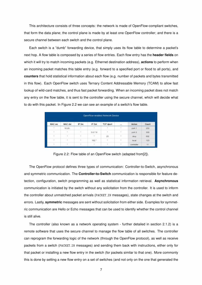
Each switch is a ”dumb” forwarding device, that simply uses its flow table to determine a packet’s

next hop. A flow table is composed by a series of flow entries. Each flow entry has the header fields on

which it will try to match incoming packets (e.g. Ethernet destination address), actions to perform when

an incoming packet matches this table entry (e.g. forward to a specified port or flood to all ports), and

counters that hold statistical information about each flow (e.g. number of packets and bytes transmitted

in this flow). Each OpenFlow switch uses Ternary Content Addressable Memory (TCAM) to allow fast

lookup of wild-card matches, and thus fast packet forwarding. When an incoming packet does not match

any entry on the flow table, it is sent to the controller using the secure channel, which will decide what

to do with this packet. In Figure 2.2 we can see an example of a switch’s flow table.

Figure 2.2: Flow table of an OpenFlow switch (adapted from[2]).

The OpenFlow protocol defines three types of communication: Controller-to-Switch, asynchronous

and symmetric communication. The Controller-to-Switch communication is responsible for feature de-

tection, configuration, switch programming as well as statistical information retrieval. Asynchronous

communication is initiated by the switch without any solicitation from the controller. It is used to inform

the controller about unmatched packet arrivals (PACKET IN messages), state changes at the switch and

errors. Lastly, symmetric messages are sent without solicitation from either side. Examples for symmet-

ric communication are Hello or Echo messages that can be used to identify whether the control channel

is still alive.

The controller (also known as a network operating system - further detailed in section 2.1.2) is a

remote software that uses the secure channel to manage the flow table of all switches. The controller

can reprogram the forwarding logic of the network (through the OpenFlow protocol), as well as receive

packets from a switch (PACKET IN messages) and sending them back with instructions, either only for

that packet or installing a new flow entry in the switch (for packets similar to that one). More commonly

this is done by setting a new flow entry on a set of switches (and not only on the one that generated the

7

PACKET IN message), which will define the flow for that kind of packets. The controller is also able to

create a packet from scratch (i.e. without any event generated by a switch), and send it to one or more

switches, through PACKET OUT messages.

OpenFlow versions: The OpenFlow 1.0 specification [1] is currently the most widely used throughout

the world [33]. As of the writing of this thesis, the most recent OpenFlow specification is version 1.4 [3].

In the OpenFlow 1.0 specification (the first non-draft version) the switch can process 12 header fields

(for instance Ethernet, IP, TCP and UDP source and destination adresses), has only one flow table and

can only connect to one controller. Along the years, with the evolution of the protocol, the OpenFlow 1.4

specification allows an OpenFlow switch to process, among others, IPv6, ICMPv6 and MPLS headers.

It also introduces the OpenFlow Extensible Match, which drastically changes how packet matching is

made and allows the definition of new match entries in an extensible way. Another improvement are: the

support for multiple flow tables (and also groups of tables), which eases the implementation of complex

forwarding tasks (such as multipath); and the switches’ ability to connect to multiple controllers at the

same time, which enhances scalability and fault tolerance.

OpenFlow began with a very basic support for Quality of Service (QoS). As the implementation of

QoS mechanisms are very vendor specific, the protocol has to be general enough to cope with all these

different mechanisms and hardware. In version 1.0, the protocol defines the creation of queues, with

minimum rate as its only parameter. Instead of forwarding directly to a port, one can define the flow

entries on a switch to forward to specific queues (with enqueue action), each with its own minimum

rate. One switch port can contain one or several queues. On version 1.1 it was added the ability to

process MPLS labels. On version 1.2, each queue can also have a maximum rate. The version 1.3 of

the specification brought an important improvement for QoS enforcement, which is the meter table. This

table contains per-flow meters that measure the rate of packets attached to each flow (as opposed to

queues that are attached to ports). This new feature combined with queues allows the implementation

of complex QoS frameworks [3], such as DiffServ (Differentiated Services).

It is important to refer that through the OpenFlow protocol the controller can only query information

about the queues of a given switch, but not modify it, as it is out of scope of the OpenFlow specification

[3]. To achieve this, the ONF created the OF-CONFIG protocol [4]. Using this protocol, one can config-

ure the queues of a switch, but also other parameters not defined by the OpenFlow protocol, such as

ports parameters or the administrative controller for a switch. The version 1.0 of OF-CONFIG requires

switches with OpenFlow 1.2 or later. As of this writing, the latest version of OF-CONFIG protocol is 1.2

[4], which supports switches up to version 1.3 of OpenFlow.

8

2.1.2 OpenFlow Controllers

Gude et al. published the first OpenFlow controller - NOX [21]. The authors of this work identify the

need for an abstraction to the management of networks, making an analogy to operating systems. In

the early days of computing, programs were written in machine language and as a result they were hard

to deploy, port and debug. Operating systems created an abstraction layer to the physical resources,

which enhanced productivity and enabled programs to run independently of the underlying physical

resources. The controller aims at providing this abstraction for networks, becoming itself a centralized

control plane (and hence decoupling from the data plane), and being responsible for controlling the

switches logic (using the OpenFlow protocol described in the previous section). This abstraction eases

policy enforcement and increases optimal resource management, since applications running on top of

a network operating system can get the ”big picture” of the network (network-wide view), as opposed to

current network management done by distributed low-level algorithms.

Industrial OpenFlow Controllers: Since the release of NOX a great number of other OpenFlow con-

trollers have been developed. Mainly they fall into two classes: closed-source commercial controllers;

and open-source research and community oriented controllers. Examples of the former are Big Network

Controller 1 from Big Switch Networks, Onix [30] from Nicira Networks (now owned by VMWare) and

Contrail2 from Juniper. Examples of the latter are: Trema and MUL (C based); Beacon [19] and Flood-

light 3, a fork of Beacon (Java based); POX, Pyretic, and Ryu (Python based). OpenDaylight [35] is a

Java based controller that can be seen as belonging to both classes, since it is an open-source project

hosted by the Linux Foundation, but at the same time is supported by the networking industry with con-

tributions (of both code and resources) from several companies. It is the first controller that supports

communication with the switches (known as the southbound interface) not using the OpenFlow protocol

(e.g. using NETCONF [17]).

The Beacon controller was one of the first ones to appear (after NOX) and its source-code was the

basis of both Floodlight and OpenDaylight. However, natively Beacon does not support topologies with

loops in it, making it more difficult to work with. Beacon is no longer in development. Both Floodlight

and OpenDaylight support topologies with loops and both are in active development and with great

acceptance by the community. They were both considered as an option to be used in our work, but the

choice fell on Floodlight, with the justification presented in section 3.1.

There has been some research work on how to evaluate the performance of SDN controllers. In

[45], Tootoonchian et al. propose Cbench, a benchmarking tool for SDN controllers that emulates a1http://bigswitch.com/products/SDN-Controller (Last Access: 15-05-2015)2http://www.juniper.net/us/en/local/pdf/whitepapers/2000515-en.pdf (Last Access: 15-05-2015)3http://www.projectfloodlight.org/floodlight/ (Last Access: 01-10-2015)

9

http://bigswitch.com/products/SDN-Controller

http://www.juniper.net/us/en/local/pdf/whitepapers/2000515-en.pdf

http://www.projectfloodlight.org/floodlight/

given number of OpenFlow switches that generate traffic to the controller to measure its performance.

Performance metrics of Cbench are the throughput (events per second that the controller can handle)

and the response latency (time to answer to a switch’s request). Shalimov et al. created Hcprobe

[39], a tool that is based on Cbench with some extra functionalities. The authors of Hcprobe state that

previous evaluations of SDN controllers were only focused on performance. Thus, for reliability testing

Hcprobe can measure the number of controller failures in a long-term run, and for security evaluation

it tests if the controllers process correctly malformed OpenFlow packets and headers. Both of these

works use their tools to make performance analysis on several OpenFlow controllers (presented in the

previous paragraph), concluding that Beacon is the controller with the highest performance (confirming

the results shown in [19]) The Python based controllers showed the worst performance, since they can

only run in a single thread. Due to OpenDaylight recent publication date, as of this writing there was no

evaluation work considering the OpenDaylight [35] controller.

Research OpenFlow Controllers: While having a centralized control plane brings many benefits to

network management, it also raises several concerns regarding the scalability, robustness and reliability

of the controller in large scale networks. Heller et al. worked on the controller placement problem [27],

which studies the number of controllers needed and respective location for different topologies. The cor-

rect position is calculated by solving an optimization problem for a predefined metric (average or worst

case latencies in their proposal) from all nodes in the network to the controller. They concluded that for

most topologies, there is only need for one controller as long as it is correctly positioned. To address

control plane failures, two distributed control plane approaches have been proposed: Tootoonchian et

al. presented HyperFlow[44], based on a publish/subscribe system between the controllers, which prop-

agate events between them to maintain a consistent state among different controllers. An OpenFlow

switch connects to one controller only, but any controller in the network can control any switch, by in-

tercepting messages that travel on the network and issuing new events in the control plane directed to

an authoritative controller of a given switch; The second approach is the work by Botelho et al. called

SMaRtLight [11]. In this case each switch connects to the same controller, and there are backup con-

trollers that can take the primary role in cause of failure. The primary and backup controllers have a

shared data store, implemented as a Replicated State Machine, in order to keep the state consistent

among controllers. SMaRtLight shows only a preliminary evaluation, testing the throughput of the pro-

posed controller as the works referred in the previous paragraph. HyperFlow also shows a rudimentary

evaluation, describing only the tests procedure and stating that HyperFlow can withstand a level of dy-

namism of the network of up to 1000 changes per second in the network (links up/down or switches

joining/leaving).

10

2.1.3 OpenFlow Network Simulators/Emulators

In this section it is explored the most relevant network simulators/emulators for this work. The widely

known network simulator ns-3 [28] has support for an OpenFlow simulation model4, however its current

implementation does not model the OpenFlow controller as an external entity, therefore it does not

support simulating multiple switches connected to an OpenFlow controller. Thus it does not allow to

simulate a software-defined network with a controller dynamically changing the behaviour of the network

elements.

Mininet 1.0: Lantz et al. developed Mininet [32], a network emulator system for prototyping large net-

works on the constrained resources of a single laptop. Mininet uses lightweight virtualization to scale

to large topologies. The file system, kernel, device drivers, and other common code are shared be-

tween processes and managed by the operating system. It virtualizes the nodes by creating a different

network namespace (i.e. a container for network state) for each host, which gives each one their own

virtual Ethernet interface. The links are virtual Ethernet pairs (veth pairs), which makes virtual interfaces

appear as a fully functional Ethernet port to all system. Mininet supports both user and kernel space

virtual switches, such as the OpenFlow reference switch [3] (user space) and Open vSwitch [36] (user

and kernel space). Open vSwitch consists in a virtualized switch, making it possible to deploy/remove

or scale up/down according to the needs of the administrator. Mininet supports changing dynamically

the network topology (i.e. links can be set to up/down and hosts can crash) and as this is an emulated

environment, the authors state that the experiments made on Mininet can be ported to hardware seam-

lessly. The Mininet paper [32] indicates that one can create a network of 1024 hosts and 32 switches

using 492 MB of RAM.

Mininet 2.0 (Hi-Fi): One of the main limitations the authors presented in Mininet is the lack of perfor-

mance fidelity, especially at high loads. Since CPU resources are multiplexed in time by the default Linux

scheduler, there is no guarantee that a host that is ready to send a packet will be scheduled promptly.

So, the authors improved Mininet and presented Mininet Hi-Fi [25] (High-Fidelity). Mininet-HiFi extends

the original Mininet architecture by adding mechanisms for performance isolation, resource provision-

ing, and monitoring for performance fidelity. This is done by using the following Linux features: control

groups (cgroups), which allow a group of processes belonging to a virtual host to be treated the same

way; CPU Bandwidth Limits are enforced for each virtual host, assigning a maximum time quota (con-

figurable) for each cgroup; Each link (veth pair) is configured using the traffic control tool (tc), which sets

properties such as bandwidth or delay. Mininet Hi-Fi then constantly monitors the performance of each

4http://www.nsnam.org/docs/release/3.13/models/html/openflow-switch.html (Last Access: 09-01-2015)

11

http://www.nsnam.org/docs/release/3.13/models/html/openflow-switch.html

virtual host or virtual link, so that in the end of the experiment it is able to tell if fidelity was kept or the

experiment should be reconfigured (or scaled down). Since in Mininet the only limitation to the size of

the experiments is the underlying computational infrastructure, Wette et al. presented an extension to

Mininet called MaxiNet [51]. MaxiNet is an abstraction layer connecting multiple, unmodified Mininet in-

stances running on different computers. A centralized API (called MaxiNet API), which is very similar to

Mininet API, provides access to this cluster of Mininet instances, which allows to control the experience.

The connection between MaxiNet and Mininet instances happens through RPC calls. In this paper the

authors show that using MaxiNet with 12 computers, they were able to emulate a data center with 3600

nodes (servers and switches), maintaining the CPU usage of each computer below 80% (to compensate

for peaks in the CPU usage, which otherwise would bias the outcome of the experiment).

EstiNet: EstiNet [49], presented by Wang et al., is commercial tool that at the same time is a network

emulator and simulator. It is an emulator since every node uses the real TCP/IP protocol stack and

also the code developed in EstiNet can readily run on without any modification on a real scenario. To

address the performance fidelity, EstiNet is at the same time a simulator, having its own simulation

engine. Instead of scheduling the virtual nodes events using the underlying operating system (which

may be unpredictable), it uses its simulation engine to schedule all events according to the simulation

clock, which is slower than real time. This is done using a technique known as Kernel Re-entering, which

uses tunnel network interfaces to intercept the packets exchanged by virtual nodes and redirect them

into the EstiNet simulation engine.

Since EstiNet is based on a simulation clock, the authors claim that its results are accurate and

repeatable. One of the authors published a study [48] comparing the performance fidelity and scalability

of EstiNet versus Mininet. In this study the author evaluates both platforms creating a grid of NxN

switches (where N goes from 5 up to 31) and then testing the ping time between two hosts at opposite

edges of the grid. The author concludes that generally Mininet worked well but EstiNet gives results

closer to the theoretical ones and that they are repeatable. However, it needs more time to simulate

OpenFlow switches [48]. Nevertheless, according to [33], Mininet is the network emulator most used by

the network research community.

2.2 Strategies for Network Flow Allocation in Data Centers

We now present the classification that emerged from the study of several works regarding network

management in data centers. At the highest level, the studied works can be divided in two categories.

Thus, our taxonomy for network allocation techniques in data centers is: dynamic allocation based

12

on network monitoring; and static allocation based on virtual network embedding. The former aims

at maximizing resource utilization, fair bandwidth sharing of the physical network and sometimes give

Quality of Service (QoS) guarantees for end hosts, while the latter provides support for virtual networks

with QoS guarantees but with small (or even none) maximization of network usage. Each category is

now explained in greater detail.

2.2.1 Dynamic Allocation based on Network Monitoring

This kind of approaches rely on a constant monitoring of the network performance to keep an up-to-

date view of the data center network. For that purpose, it is periodically gathered statistical information

from the network elements (and/or end hosts), in order to infer the bandwidth usage for each VM or

physical server. With this updated view of the network, this type of systems can use traffic engineering

techniques to maximize resource utilization, leading to an economical gain for the provider, since it can

for instance aggregate requests and shut down unused resources. The maximization of resource usage

is possible since these dynamic approaches can react to the changing demands from different tenants,

and manage them to get the most of the providers’ resources. The solutions we have surveyed can be

categorized as based on: centralized traffic matrix estimation or bandwidth regulation in each end host.

Centralized Traffic Matrix Estimation: In current multi-tenant data centers there is a huge number

of different applications sharing the infrastructure, which makes demand estimation very hard since the

workload of each VM is very hard to predict. Traffic (or demand) matrix estimation approaches are based

on a central node that collects information about the state of the network to detect large flows (in terms

of bandwidth) between a certain VM/server pair. For traffic matrix estimation, all of the studied systems

follow a very similar technique. They create an N by N matrix, where N is the number of hosts in the

data center. Inside this matrix, in the row i and column j is the traffic demand from host i to host j.

Upon detecting the current demands for the data center, the central node is able to dynamically react

and place large flows on links with more capacity and aggregate as much as possible the small flows.

Examples of works that follow this idea are Hedera [6], DevoFlow [15] and MicroTE [9]. These three

works are very similar between them, thus we will only describe with detail MicroTE because it is the

most related with this work. Heller et al. presented ElasticTree [26], which as these systems is based on

traffic matrix estimation. However, the goal of the system is to know the matrix to save as much energy

as possible in the data center, which makes the system different from these since ElasticTree does not

provide neither bandwidth sharing nor bandwidth guarantees.

13

Bandwidth Regulation at End Host: Instead of monitoring the whole network and predict the current

traffic demands on a centralized node, some authors defend the idea of managing the data center’s

bandwidth in a distributed manner. In this model, each entity (e.g. a process or a VM) gets assigned a

weight (defined by the network administrator), which will be used to share the bandwidth across multiple

tenants in a proportional way. There is a congestion controlled tunnel between each pair of communi-

cating entities, that is used by the receiver to inform the sender of congestion when packets are lost.

The sender upon receiving this congestion message adjusts its rate to spare the network resources.

The mechanism proposed here is similar to Additive Increase Multiplicative Decrease (AIMD) used by

TCP in congestion avoidance. This mechanism is implemented by a rate controller in each physical

server (e.g. in the hypervisor ), which throttles the sending rate according to: the weight of each entity

as well as the congestion messages received. With this approach (and unlike the previous paragraph),

malicious tenants cannot hog the network bandwidth since the resources are fairly shared according to

the weights previously defined.

Works following this model are presented in [41, 38]. Although they are very akin to each other, they

will both be detailed in section 2.3.1, because Gatekeeper [38] has some ideas inspired from Seawall

[41], but it improves the state-of-the-art by introducing a new property (namely a work-conservative

system with bandwidth guarantees at the same time).

2.2.2 Static Allocation based on Virtual Network Embedding

A different way to allocate network resources is to use virtual network embedding algorithms. Whereas

the algorithms from the previous section aim at maximizing the resource usage and QoS guarantees for

the tenants, in virtual network embedding the aim is to completely virtualize the network, providing per-

formance isolation among tenants at the network level. So, virtual network embedding consists in the

mapping of virtual networks (consisting of virtual nodes and links) onto the substrate network (consist-

ing of physical nodes and links). Some works do not call this embedding, but are doing the same thing

(mapping virtual networks in one or more physical networks). However, the most recent papers have

used this nomenclature, which shows this name is generally accepted by the scientific community.

Virtual network embedding is the main challenge in the implementation of network virtualization [20].

In the data center context, network virtualization is advantageous because it allows clients to define

the desired network topology, which will be allocated within the infrastructure exactly as defined by the

client. This enables seamless migrations of current enterprise or scientific networks to a data center

environment, since the client defines the topology and the wanted guarantees (either CPU or bandwidth

between machines), which will be enforced by the embedding algorithm by placing the virtual network

14

only where there are sufficient resources left.

This means that virtual resources are first mapped to candidate substrate resources. Substrate re-

sources are spent (and the entire network is embedded) only if all virtual resources can be mapped.

Network embedding algorithms work similar to the Integrated Services architecture (IntServ [13]), mak-

ing reservations in the substrate network according to virtual networks’ requests. This gives strict band-

width guarantees for each tenant since each link is never oversubscribed, but can lead to poor resource

utilization as each reservation will not utilize the requested capacity all the time. This trade-off will be

addressed again in section 2.4.

The virtual network embedding problem is proven to be NP-hard (and related to the multi-way sep-

arator problem), as it deals with constraints on both physical machines and links. So, we classify virtual

network embedding systems according to if they output embedding results according to exact optimiza-

tion or if they employ some heuristic to lower the execution time (and thus give an approximate result).

We first give a formal description of the virtual network embedding problem and then describe the two

categories mentioned above.

Problem Formulation: We now describe the virtual network embedding problem in a formal manner.

Consider the following: SN = (N,L) is the substrate network, in which N is the set of nodes and L the

set of links of the network; V NRi = (N i, Li) is the set of i = 1, ..., n virtual network requests, where N i

and Li are the set of nodes and links of virtual networks request i, respectively;−→R is a vector space of

resource vectors and cap : N × L→−→R is a function that assigns available resources to some elements

of the substrate network; finally, demi : Ni×Li →

−→R is the function that assigns demands to elements of

all virtual network requests, for each V NRi. With this defined, the virtual network embedding problem

consists on the results of the functions fi : N i → N and gi : Li → SN ′ ⊆ SN . The functions fi

and gi are called node mapping function and link mapping function, respectively. The two of them

combined form the embedding for the virtual network request i (V NRi). The problem itself can then be

described as for each V NRi, these functions must comply with: ∀ni ∈ N i : demi(ni) ≤ cap(fi(n

i)) and

∀li ∈ Li : ∀l ∈ gi(li) : demi(li) ≤ cap(l). The bottom line is that the sum of each node and link demand

within the Virtual Network Requests (N i and Li) must be less or equal than the physical resources

available both for nodes (cap(n)) and links (cap(l)).

Calculation of Optimal Solution: The optimal embedding solutions can be calculated using optimiza-

tion methods, such as Linear Programming. Namely, we can use Integer Linear Programming (ILP) to

formulate the virtual network embedding problem, including both the node and link constraints in the

same formulation. Although ILP is in most cases NP-complete, there are algorithms (e.g. branch and

15

bound) that can solve the optimization problem in a legitimate amount of time. The work presented in

[29] uses ILP to solve the virtual network embedding problem. It seeks the minimization of embedding

cost and the maximization of the acceptance ratio of virtual network requests, including those criteria in

the objective function of the ILP formulation. Other example of the usage of exact formulation of ILP is

[12], which tries to make the virtual network embedding energy-aware. For that, it makes the embedding

in the smallest set of resources of the substrate network (i.e. consolidate), with the objective to shut

down unused resources (and thus save energy consumption).

In the fast-paced environment of a data center, the execution time of an algorithm is crucial, since

it limits the amount and rate of virtual network requests a provider can process. So, algorithms that

perform the calculation of the optimal solution are not suited for a data center, because it is a large

environment, giving a huge search space for the network embedding algorithm. Moreover, as in a data

center the tenants’ requests arrive in real time, we do not know the whole set of virtual networks we want

to map on the substrate network. This makes the calculation of the optimal solution possibly a waste

of time, since it can spend time calculating a optimal solutions for conditions that will change very soon

(upon the arrival of the next virtual network request). For these reasons, approaches based on optimal

solutions are not further detailed, and thus are not presented in section 2.3.

Heuristic-based Approaches: As stated in the last paragraph, the calculation of an exact solution

can be very time consuming. To deal with the NP-hardness of the virtual network embedding problem,

heuristic approaches ”trade” a low execution time for a not optimal (but acceptable) solution.

Besides low execution time, these heuristics may have many different goals. Each heuristic-based

algorithm is tailored to some specific objective as well as to some specific environment. For instance, in

[37], the goal of the algorithm is to make the virtual network embedding with fast failure recovery times,

which the authors call survivable networks. For this purpose, the heuristic used in this work is focused

on creating a link of backup paths for each substrate link (e.g. using k-shortest path [18]), which will

then give a fast re-routing of the current network embeddings when a link failure happens.

There are many other examples regarding heuristic-based approaches for virtual network embed-

ding. However, we will now focus on works that are closely related to ours, i.e., virtual network embed-

ding in data center environments. In the next section each work will be described in detail (along with

the differences between each one). However, we were able to conclude that the core of all the studied

algorithms is the same, since they all focus on delivering bandwidth guarantees in a data center network.

The heuristic these works employ to reduce the search space for a solution (and hence reduce algo-

rithm execution time) is to try to take into account server locality of the same virtual network embedding

request. Therefore, upon a virtual network request, these systems first do the node mapping, by trying

16

to accommodate everything inside a single server (if the request is smaller than the VM capacity of a

server), after that they try on servers of the same rack, then on adjacent racks, and so on.

The choice of the first server rack to analyse varies from work to work, but it is either random or in

a round-robin fashion. The link mapping phase only starts if the virtual network request completes the

node mapping phase. If it does not, it can be put into a queue to be processed later or the request

discarded to alert the client there are not resources available for his request.

Thus, in the link mapping phase each node of the virtual network is already mapped to a substrate

VM. The problem is now to connect these VMs according to the bandwidth requirements. To accomplish

this, some works use the k-shortest path algorithm [18] (increasing k until the bandwidth available com-

plies with the request), while other works use the widest shortest path algorithm [50] to provide a path

with the required bandwidth.

This kind of algorithm can be called greedy, since it picks the locally optimal choice at each branch

in the road (i.e. it chooses the best solution that complies with the virtual network constraints). With this

type of algorithms the virtual networks also benefit from the reduced number of hops in the substrate

network, which will yield low latency (as much as possible, but with no guarantees) between the VMs

communicating in the virtual network. Some works following this approach can be seen in [24, 8, 7, 53,

54]. Although these are all based on heuristics, the work from Yu et al. [53] does not reduce significantly

the search space for a virtual network embedding solution, since it considers path splitting (i.e. bifurcated

traffic) and migration of VMs at the same time. This results in a solution only appropriate for small data

centers, since it produces results in a reasonable time only when there are tens to hundreds of nodes in

the network. We will further detail in section 2.3.2 Oktopus [7] and SecondNet [24], as these have the

most interesting properties and/or implementations to discuss.

2.3 Relevant Related Systems

We now describe the works most related with this thesis. Whereas in the previous section we have

outlined the common characteristics of the surveyed works, we now detail the most relevant works,

showing the particularities of each one. As in section 2.2, we will divide this section in: dynamic allocation

based on network monitoring; and static allocation based on virtual network embedding.

2.3.1 Dynamic Allocation based on Network Monitoring

MicroTE: This system [9] uses OpenFlow as a framework to have centralized control over the data

center and make routing decisions based on predictions of the traffic matrix. Based on measurements

17

made by the authors, they state that current traffic engineering techniques do not apply well to a data

center, because they are too slow to react to micro-congestions. Therefore, the authors indicate that

the reaction time must be under 2 seconds to be effective. For this purpose, they create a hierarchical

structure to make traffic measurements that is scalable both with the data center size and with having a

centralized controller.

This works as follows: on each rack, there is a server (called the designated server) that is respon-

sible for collecting statistics from all servers in that rack every 0.1 s and also calculating the mean of the

traffic demand for each pair of servers. This designated server then receives this demand and computes

the new traffic matrix. If the average and this new value are within δ of each other, the designated server

does not do anything (the authors empirically determined δ to be 20%). Otherwise, the designated

server sends summarized information about the traffic demands (i.e. only the positions of the matrix that

changed at least 20%) to the centralized controller.

With this structure, the controller only receives information about the traffic demands when they

change, which decreases the amount of control traffic in the network. So, it is able to react to changes

in a reasonable time, reconfiguring the network elements to place each demand in a link that best fits it.

To determine this reconfiguration of the network, the centralized controller has a routing engine that can

implement several routing algorithms, according to the preferences of the administrator. As an example,

the authors describe a bin-packing heuristic they implemented in the routing engine. It begins by sorting

the demand pairs in decreasing order of traffic volume. For each pair, it is computed the minimum cost

path between them, where the cost of each link is the reciprocal of its available capacity. After assigning

the traffic of a demand pair to a path, it is updated the cost of each link along the path by deducting the

pair’s traffic volume from the residual capacity of the corresponding links. In this way, a highly utilized

link is unlikely to be assigned more traffic and the maximum link load will be minimized.

Seawall: Seawall [41] tackles the problem of fair bandwidth sharing and network performance isolation

in data centers. Current data centers have strong performance isolation at the VM level (CPU, memory

and so on), but they lack performance isolation at the network level, since an increase of a VM’s band-

width usage can lead to an decrease in performance of other VMs. The authors of Seawall propose

to overcome this problem by assigning weights to each entity (can be a VM or a process inside a VM).

Then, the share of bandwidth obtained by the entity in each network link is proportional to its weight.

To accomplish this, Seawall relies on congestion-controlled tunnels created between each pair of

source and destination VM. This is implemented at each server in a shim layer, which forces each VM

to use these tunnels. Sequence numbers are added to each packet sent trough the tunnel. These

sequence numbers are stripped at the destination server and are used to detect packet losses due to

18

network congestion. Upon receiving congestion notification messages from receivers, senders use in-

formation from network topology to detect bottleneck links and adjust transmission rates at tunnels using

that link. The adjustment is computed at each end host and is proportional to the weights associated

with VMs sending traffic to that link. Rates are adjusted using weighted AIMD functions, as in TCP.

Since the main block of this system is the rate-limiter at each host, Seawall works irrespective to the

data center topology and the communication protocols used by the VMs. It also achieves high scalability

by maintaining the state distributed in each host. However, the hosts need updated information about

the network topology so that Seawall can work, and the authors do not specify how this works. They

relegate the updated topology dissemination problem to management software that is responsible for

provisioning and monitoring the servers, and propose to use traceroute in case this software does not

provide this.

Gatekeeper: Gatekeeper [38] is a system similar to Seawall [41], but providing minimum bandwidth

guarantees. The authors recognize that Gatekeeper shares some design ideas with Seawall, but they

extend them to achieve different goals.

Namely, Gatekeeper uses Open vSwitch [36] in each server to control all the VMs within a server.

Each VM has a vNIC (virtual network interface card), that connects to the Open vSwitch. To each VM is

assigned a minimum receive bandwidth guarantee as well as a minimum send bandwidth guarantee (it

can also be assigned a maximum bandwidth for each VM). Minimum bandwidth guarantees are achieved

using an admission control mechanism that limits the sum of guarantees to the available physical link

bandwidth.

On the sender side, transmission bandwidth scheduling is done using a traditional weighted fair

scheduler that provides these guarantees. On the receiver side, Gatekeeper monitors the receive traffic

rate at each vNIC (and also the physical link) and determines the receive bandwidth allocation to each

vNIC at periodic intervals (10 ms in the authors implementation), taking into account the link usage and

the minimum rate for each vNIC.

If a vNIC receive bandwidth exceeds its computed allocation, Gatekeeper sends a feedback message

to other remote Gatekeeper instances hosting VMs contributing to its traffic. The feedback message in-

cludes an explicit rate that is computed by distributing the desired vNIC receive rate among the senders.

A feedback message is generated if the aggregate rate on the physical link exceeds a given threshold

(95% of the link bandwidth in their implementation) or if a vNIC exceeds its predefined maximum rate.

This message is the equivalent to the congestion message in Seawall, except in this case is to control

the rates that are operating above predefined allocation. In this way, the system throttles the misbehaved

VMs right away, which avoids congestions in the data center.

19

Also, each vNIC can exceed its guaranteed allocation when extra bandwidth is available, which is

implemented by the weighted fair scheduler in the virtual switch (Open vSwitch). This is important in

order to maximize resource utilization, since with a static allocation (for minimum bandwidth guaran-

tee) the resources could be idle, resulting in economical losses to the resource provider. Although the

Gatekeeper idea of mixing guarantees with a work-conservative system is very promising, it is yet to be

determined its performance under a realistic scenario, since the authors only evaluated this work with

two tenants and six VMs, postponing to future work an evaluation in a different data center environment

(larger configuration and dynamic workloads).

2.3.2 Static Allocation based on Virtual Network Embedding

Oktopus: The authors of Oktopus [7] affirm that the unpredictability of network performance in data

center environments is damaging both tenants and service providers, since the tenants’ applications

suffer from this unpredictability and the service provider can incur in avoidable revenue losses. So, their

work is intended as a move towards predictable networks, giving network guarantees to tenants.

In Oktopus tenants require a virtual cluster, defining the number of VMs and the bandwidth desired

between them (e.g. <3, 100> means 3 VMs with a 100 Mbit/s connection between them). Tenants can

also require a oversubscribed virtual cluster, where the links are oversubscribed and the guarantee is

weaker, but with the advantage of lower cost. Upon receiving a request, Oktopus relies on a central

node that does the embedding of this request onto the physical network. The algorithm running in the

central node tries to do the embedding in the smallest sub-tree possible, starting in the same machine,

then on the same rack and so on, checking at each stage if this sub-tree complies with both VMs and

networking requests. This makes this system only applicable to data centers with tree-like topologies.

The greedy algorithm to the oversubscribed virtual cluster is the same, but with the constraints on the

links less severe (according to an oversubscription factor). Oktopus makes static allocations, which does

not allow one tenant to use more bandwidth than what was defined in the request, even if it is free. To

enforce this, it employs a rate-limiter in the hypervisor of each physical machine, throttling the bandwidth

of each VM according to what was allocated.

SecondNet: This work [24] has the same structure as the one presented in the previous paragraph,

i.e. a central unit that receives virtual network requests to process and allocate. SecondNet uses the

central unit to run the embedding algorithm, so that it outputs the physical machine of each VM and the

routes between VMs. But, unlike Oktopus, these routes calculated by the central node do not translate

into routing rules to the switches because in SecondNet the physical machines keep information about

20

the routes of each VM it owns. The authors name this Port Switching Source Routing (PSSR) and it

consists in injecting in each packet a list of output switch ports the packet will go through.

When a packet arrives to a switch, the switch pops the first element of this list, getting the output port

to forward this packet. The next switch receives the list with one element less and applies the same pro-

cedure. With this approach the switches are stateless, passing this responsibility to the physical servers

(making the system more scalable). Similar to Oktopus, SecondNet throttles VM traffic at the hypervisor

to provide guarantees and performance isolation. But in SecondNet this throttling is not limited to the re-

quested bandwidth, and the authors introduce three traffic levels (with decreasing priority): guaranteed

bandwidth, guaranteed bandwidth on first and last hop, and best-effort. The best-effort traffic is only

routed when the other two types of traffic are not using the entire bandwidth. This is not fair bandwidth

sharing as presented in 2.2.1, but it is better than static reservations with no bandwidth sharing.

Regarding the allocation algorithm running on the central entity, it also tries to embed each request

on the smallest subset possible (same machine and so on). But SecondNet does not use a sub-tree

to check if the request can be mapped to these physical resources. Instead, it builds a bipartite graph,

with VMs on one side and physical servers on the other, adding edges to the graph for matching pairs

of <VM, Physical Server>. This makes the SecondNet system independent of the physical topology of

the data center, making it deployable in more environments.

The authors also present (but do not detail) a second algorithm that runs periodically and is respon-

sible to consolidate the VMs of the same virtual network as close as possible. The algorithm checks

the virtual networks that are more scattered across the physical network and sees if it is possible to

migrate some VMs to make the virtual network smaller (in terms of path lengths). The authors further

state that this is a process that can be running in background when the load of the VMs to be migrated

is low. However, this can lead to waiting too long for a certain VM load to get low, possibly causing the

migration adverse (or inapplicable) at that time.

2.4 Summary and Final Remarks

After the classification and description of the related work throughout this section, we now present a

table (Table 2.1) that shows a comparative analysis of the systems and solutions we have studied.

The criteria present in Table 1 is the criteria we have been discussing throughout this section and

needs no explanation. Regarding the ”Partially”, each one was explained appropriately when the corre-

sponding system was being described.

Other than that we can see that each system has its focus on a certain area, providing the set of

properties ”expected” for that kind of system. The first four rows of this table are the system that employ

21

SystemEnd-to-endBandwidthGuarantees

Work-Conservative

Supportfor VirtualNetworks

Support forConsolida-

tion

OptimizationTechnique

Scalable toData Center

Size

De-voFlow No Yes No No Not

Applicable Yes

Hedera No Yes No No NotApplicable Yes

MicroTE No Yes No No NotApplicable Yes

Seawall No Yes No No NotApplicable Yes

Gate-keeper Yes Yes No No Not

Applicable Yes

Houidi etal. Yes No Yes No Exact No

Botero etal. Yes No Yes Yes Exact No

Yu et al. Yes No Yes Yes Heuristic-based Partially

VDCPlanner Yes No Yes Yes Heuristic-

based Yes

Cloud-NaaS Yes No Partially No Heuristic-

based Yes

Oktopus Yes No Yes No Heuristic-based Yes

Second-Net Yes Yes Partially Yes Heuristic-

basedYes

Table 2.1: Comparative analysis of the studied systems.

22

a dynamic allocation that is based on network monitoring. None of these systems provide bandwidth

guarantees, but they are work-conservative systems, since they foster fair bandwidth sharing among

tenants. The other eight rows of this table show systems that perform static allocations based on virtual

network embedding. These systems provide bandwidth guarantees for their tenants and most of them

support consolidation of the virtual networks they allocate.

The most ”all-around” system, and also the most similar to the solution we present in the next chapter,

is SecondNet. We can see that it has almost all the properties presented in the table, with exception for

supporting virtual networks, because they only employ classes of traffic (i.e. a tenant can not ask for an

exact bandwidth guarantee). Another difference is the approach regarding consolidation. They employ

an algorithm that runs periodically, while we do the consolidation incrementally, upon the reception of

each request.

23

Chapter 3

omniCluster

We now present and describe our solution - omniCluster. We begin by providing a generic use case

for our system, in the following paragraphs. Then, in section 3.1 we provide a detailed architecture

description, focusing on the interactions between each component of our solution. In section 3.2 we go

in-depth to the components presented in the previous section, and describe the internal working of each

one. Then, in section 3.3, we give some concluding remarks regarding our solution and summarize what

has been described in this chapter.

In Figure 3.1 we can see the high level architecture of the solution, in this case using a simple tree

topology with depth equal to 3 and fanout equal to 2. Although many topologies are being proposed by

the network research community, we will focus on the traditional tree-like topologies (Tree and Fat-tree)

since they are still the most used data center topologies, as described in [10]. The OpenFlow controller

(in the top-right corner) is the central component of the solution, as it is responsible for running the virtual

network embedding algorithm in order to map the requests on the substrate network, and then program

the switches to deploy the requested virtual networks.

As explained in section 2.1, each switch acts merely as a packet forwarder, according to the rules

dictated by the controller. The controller has a connection to every switch in the network, represented

by the dashed red lines that form the control plane. They are dashed to represent the logical (and not

physical) separation between the data and the control planes. The control plane does not necessarily

need dedicated connections, it can use the same physical links of the data plane.

As in most of the works described throughout the previous chapter, our network embedding algorithm

tries to allocate the requests on the smallest available subset of the substrate network (i.e. on the same

physical server, then on the same rack, and so on). Thus, we aim to maximize the proximity of VMs

belonging to the same tenant, which results in minimizing the number of hops between those VMs.

This is advantageous for two reasons: first, with less hops the delay is normally reduced; and second,

25

keeping the VMs close (e.g. in the same rack) relieves the bandwidth usage in the upper links of the tree,

which in the data center is where the bandwidth is scarcer[10]. With this approach, we will be able to

accept more virtual network requests, since the core links will not be so likely to become the bottleneck

of the data center.

In Figure 3.1, we can see an example of the placement of three virtual networks according to this

algorithm. The virtual network of tenant A represents the best case possible where all the VMs of the

virtual network can be mapped on the same physical server. In this case, there is no usage of the

network (which saves bandwidth for future requests), and the bottleneck of the virtual network is only

the speed within the server. In the virtual network of tenant B the request could not be mapped to a

single server, and so it uses another server belonging to the same rack to accommodate the entire

request. The virtual network of tenant C shows a case where the virtual network could not be mapped

in the same rack, and has to use a server on the adjacent rack. As we can see, the bandwidth of the

links on the top of the tree is only used in the worst cases (i.e. when the request is large or the data

center is operating near saturation).

Figure 3.1: High level architecture of the solution with a tree topology.

Besides the network embedding algorithm, that ensures the network can provide the bandwidth

26

guarantees requested by each tenant, we make use of the centralized information in the controller to

provide two properties not seen in the surveyed network embedding systems: fair bandwidth sharing

(i.e. work-conservation) among tenants (non-existent in network embedding systems) and incremental

consolidation of virtual network requests. The first is achieved by instructing every switch used by a

virtual network (which is determined by the embedding algorithm) to create a new queue for that virtual

network. As described in 2.1, the queues in OpenFlow are used to provide QoS guarantees (in this case

bandwidth). This will be discussed in detail below in section 3.2.2. The second property is enforced in

the network embedding algorithm itself (described in detail in the section 3.3), choosing the location of

a virtual network according to a best-fit heuristic on the VM placement. To do this, the algorithm needs

the current state of the network and the physical servers (which is kept by the OpenFlow controller -

detailed in section 3.2.1). By managing all this information centrally, the controller could become itself

the bottleneck of the network. However, as discussed in section 2.1.2, the controller does not need to

be a single machine. For instance, it could be a cluster of powerful machines, or we could have several

controllers controlling only a subset of the network, as proposed by [40].

3.1 Detailed Architecture

We will now describe in greater detail the architecture shown in the previous section. Figure 3.2 is

the result of ”zooming in” in each component of Figure 3.1. Thus, Figure 3.2 contains the software that

will run in each component as well as the most important interactions between those components.

Figure 3.2: Software architecture of the components present in the solution.

27

First we justify our choices regarding the components shown in Figure 3.2. For the OpenFlow con-

troller, we will use Floodlight for two reasons: first because it is based in the Java programming language,

which as shown in chapter 2 gives a good enough peformance (i.e. a little worse than controllers that

are written in the C programming language, but much better than the ones written in python, ruby and

javascript); and second because it is the most robust and stable Java-based controller. We thought

about using OpenDaylight but we felt that it is still immature, since we could not use it even in the sim-

plest scenarios. Regarding the other components, Switch and Physical Server, the choices are Open

vSwitch and Linux Process (respectively) because this solution will be implemented within the Mininet

emulator, that uses those components. We will use Mininet both because it is open-source (which is

very useful in research) and also because it is the de facto standard of OpenFlow emulators, as stated in

section 2.1.3. It is also important to refer that all the source code that will be developed could be ported

to a physical data center with few (or no) changes. The only exception is in the Linux Process, which

in a real scenario would be running an hypervisor software to manage the VMs inside that host. In this

work this is simplified to an operating system managing processes, where each process will simulate a

VM (as detailed in section 3.2.3). Another important detail is that we assume all the physical servers

have equal CPU, so that in a virtual network request a tenant asks for a percentage of a CPU (instead

of a CPU with a certain frequency, as in real data centers).

We now describe the typical flow of information when the system is in operation. First of all, the ten-

ant expresses its demands in a virtual network request (which consists in a XML file). This consists in

defining two things: the number of VMs required (and also the percentage of CPU of each one) as well

as the bandwidth required between the VMs that will be connected (expressed in MBit/s). This request

is fed into the virtual network embedding algorithm (detailed in the next section), that is running in the

OpenFlow controller. Upon receiving the request, the embedding algorithm contacts the network infor-

mation manager to get the current state of the network. Based on this state, the algorithm determines

(if the request is accepted) where this virtual network will be allocated. It is important to note that as

all the requests are processed by the controller, this updated view of the network involves zero control

messages over the network (both to switches and hosts), since the controller just has to update this

information when it processes a new virtual network request. This update, and all the data structures

that are involved in it, are detailed in section 3.2.1.

The controller then translates the resulting decision of the algorithm (i.e. the affected switches and

hosts) to OpenFlow rule(s) to reprogram the switch(es). Upon receiving this message, the Open vSwitch

manager takes two actions: creates a new queue for this virtual network, with the assured bandwidth

present in the received message; and installs a new rule in the switch’s flow table to forward packets

28

from a certain VM to the newly created queue. This means that there will be one queue for each pair of

linked VMs in a virtual network. In this way, a VM can use more bandwidth than its minimum when the

link is not throttled.

Moreover, the sharing of bandwidth between queues is made fairly according to the minimum band-

width a queue has (a queue with a higher minimum bandwidth will use more spare bandwidth). Thus, the

resource usage is maximized, since the tenants share unused bandwidth fairly, but at the same time get

their minimum bandwidth guarantee when the network is saturated. If the network is saturated, packets

may be dropped at the switch if a virtual network is generating more traffic than what it asked for. This

ensures performance isolation at the network level. As the Open vSwitch is based on the Linux kernel,

we will use the traffic control utility HTB (Hierarchical Token Bucket) to make the configuration of the

above mentioned queues. This will be explained thoroughly in section 3.2.2.

As already mentioned, the VMs will represented by and implemented as Linux processes. To simu-

late tenants’ workloads, each process will be running a traffic generator. As depicted in Figure 3.2, upon

the necessary configurations, each process (i.e. VM) can communicate with other processes on the

same virtual network, using either the operating system (in case the processes are on the same server),

or contacting its adjacent switch, which will use the flow table to check to which queue it should forward

this solicitation (in case the processes are on different servers). In this work we will only focus on com-

munication inter-server (as the intra-server communication would be a responsability of the hypervisor

in a real deployment).

3.2 System Components

Given the detailed architecture described in the last section, we now focus on each component of our

solution. As we can see in Figure 3.2, our system has three main components: the OpenFlow controller;

the OpenFlow switch; and the physical server. In the following subsections, the funcitioning of each

component is defined in greater detail.

3.2.1 OpenFlow Controller - Floodlight

As stated above, the OpenFlow controller is the most important component of our solution. It is in

the controller that resides the all the ”intelligence”, since it will run the algorithm that allocates virtual net-

works onto the physical network. Thus, we begin by showing the virtual network embedding algorithm,

describing its rationale along the way. Then, we make a descripition of the important data structures on

which the algorithm is based on, and we also make an analysis of some trade-offs inherent to some data

29

structures. We then finalize this sub-section by specifying an important design decision of our solution:

how a virtual flow (i.e. between two VMs) is defined and how it is characterized at the network level.

3.2.1.1 Virtual Network Embedding Algorithm

We now show the pseudo-code of the virtual network embedding algorithm that will be running on the

OpenFlow controller. The main guidelines of the algorithm were already explained, but now we explain

it in greater detail and formalism.

Algorithm 1 Virtual Network Embedding AlgorithmInput: VNR (Virtual Network Request)Output: True if request is accepted, False otherwise.1: totalVMLoad← getVMLoadFromVNR(VNR)2: highestCPUAvailable← getMostFreeCPU()3: if totalVMLoad < highestCPUAvailable then4: appropriateList← findAppropriateList(totalVMLoad)5: for each server in appropriateList do6: serverCPUAvailable← getCPUAvailable(server)7: if totalVMLoad < serverCPUAvailable then8: allocVirtualNetwork(VNR, server)9: return True

10: else11: server← getMostFreeServer()12: firstServer← server13: sortedVNR← sortVNRByBWDemands(VNR)14: [preAllocatedVMs, remainingVMs]← splitRequest(sortedVNR, highestCPUAvailable)15: VMsAlreadyAllocated← (preAllocatedVMs, server)16: preAlloc(preAllocatedVMs, server)17: while True do18: server← getNextServer(server)19: if server is firstServer then20: cancelAllPreAllocs()21: return False22: CPUAvailable← getCPUAvailable(server)23: [preAllocatedVMs, remainingVMs]← splitRequest(sortedVNR, CPUAvailable)24: BWDemands← calcSumOfDemands(sortedVNR, VMsAlreadyAllocated, preAllocatedVMs, server)25: linksResidualBW← calcResidualBW(VMsAlreadyAllocated, server)26: if BWDemands > linksResidualBW then27: clearLastSplitRequest()28: continue29: else30: preAlloc(preAllocatedVMs, server, BWDemands)31: VMsAlreadyAllocated← VMsAlreadyAllocated + (preAllocatedVMs, server)32: if remainingVMs is empty then33: allocAllPreAllocs()34: return True

As stated earlier, the virtual network embedding has two objectives to fulfil: to guarantee that every

VM pair in the virtual network request gets (at least) the requested bandwidth; and also to consolidate

the virtual networks on the least amount of physical resources possible. Instead of making a consoli-

dation algorithm that runs periodically, we have opted to take a new approach and do the consolidation

incrementally (at each request), merging the network embedding and the consolidation algorithms into

one. In this way, we avoid heavy migrations of VMs between servers, which would stop temporarily the

work of those VMs and also possibly generate a lot of control and data traffic. Another advantage is that

we relieve the controller from running this algorithm periodically, which would diminish its performance

when processing new virtual network requests.

To explain the rationale behind the algorithm, we will divide it in two cases: when the virtual network

request fits in on physical server and when it needs to be spread across multiple servers. This is the

30

first check made, comparing the total CPU load requested with the highest CPU available at the moment

(line 3).

If the request fits in one server, we want to find the server with the least free CPU that fits the request

(i.e. best-fit). After finding that server, we allocate this request on it (which includes updating the network

state with this new request). To find best-fit server, we first find in which set we will search in (line 4). We

will maintain 10 sets: the first keeps the servers with 0 to 10 % of CPU free, the second the servers with

10 to 20 % of CPU free, and so on. This is just to reduce the search space for the appropriate physical

server, which in a large data center environment can reduce the run time of the algorithm considerably.

If the request does not fit in one server, we sort the request by decreasing bandwidth (line 13), and

allocate as much VMs as possible in the most free server on the entire data center. In this way, the

most consuming demands are on the same physical server, which significantly relieves the load on the

network (and thus we can accept more virtual network requests). After pre-allocating (since the request

can be rejected) what is possible on the most free server, we try to allocate the rest on adjacent servers.

In line 18, the getNextServer(server ) function returns the servers on the same rack of server, then the

servers on an adjacent rack, and so on. Next we check if we already tried on every server of the data

center (line 19), and reject the request if so (cancelling all the pre-allocations).

In the next lines (22-25), we see if the server we are checking has connection(s) with sufficient

bandwidth (as defined in the request) to the other server(s) already pre-allocated in previous iteration(s).

If it does not have enough bandwidth, we try on the next server (lines 26-28). If it does, we pre-allocate

the VMs mapped onto this server. Finally, we check if the set remaining VMs to be allocated is empty

(lines 32-34): if it is we allocate all the pre-allocations (i.e. commit) and return True; if it is not, we move

on to the next server to allocate the remaining ones.

As we can see by the description of the algorithm, we will have high consolidation (and consequently

low fragmentation) of VMs within the servers, since the algorithm either allocates a whole server (if the

request does not fit one server), or finds the best-fit server (if the request fits in one server).

3.2.1.2 Relevant Data Structures

Being the algorithm thoroughly described in the preceding paragraphs, it is now necessary to de-

scribe and analyze the data structures that support it. We will divide the data structures in two groups:

the ones that are global and are always present; and the ones that are local and only exist when a virtual

network request is being processed. We think that is very important to do this disction, because the data

structures from the first group are global and thus will grow both with the size of the data center and

also with number of requests, whereas the data structures from the second group have a limited scope,

31

which means that once a virtual network request is processed, they will be garbage collected and will

not grow indefinitely. Of course it is important to treat all the data structures in the best way possible

and to implement them according to all best pratices, however we think that the global ones should be

addressed right from the design phase, since this way some bottlenecks can be avoided.

Global Data Structures:

• freeCPUOnServer - This data structure is a Map, where the key is a physical server and the value

is the percentage of free CPU on that server. This Map is a core data structure of our algorithm,

since it will define if a certain VM (or group of VMs) can be allocated in a certain server.

• NthCPUInterval - This item is actually a group of data structures, rather than just one. As previously

described (and shown in line 4 of Algorithm 1), we will keep 10 sets, where the first set contains

the servers that have between 0 and 10 percent of CPU available, the second set contains the

ones that have between 10 and 20 percent of available CPU, and so on. So, in this case, N goes

from 1 to 10. These data structures are Sets, since duplicated values can not exist (both intra and

inter Sets).

These Sets are important because the Map described in the previous bullet point will have as many

keys as physical servers in the Data Center. As in some real-world Data Centers there are up to

80000 servers1, the queries on this Map have to be well thought. We do not want to sweep all keys

of the Map, since it can seriously affect the performance of the OpenFlow controller.

Thus, these Sets are important and can improve performance in the two scenarios of the algorithm:

when a virtual network request fits within one server; and when a virtual network request has to be

splitted among different servers. In the first case, we want to find the best-fit server to our request,

i.e. we want the server which has the lowest δ to the CPU sum of the request. So, instead of

searching all the servers for this ideal server, we will only look for the hosts that are in the Set that

corresponds to the CPU sum of the request. In the second case, we want to find the server that

has the most free CPU, so that we allocate as much as we can on it, and then try to allocate the

rest on its neighbors. In this case, the Sets help again because they refrain us from searching

across all the physical servers present on that Map. Instead, we search for servers in each Set in

descendant order. We first try on the 90% to 100% Set, if it is empty on the next Set, and so on.

It is important to refer that there is a trade-off in the utilization of these Sets. One can diminish

the size of each Set, making the search in each one faster since it would have fewer elements.

However, this would come at the cost of extra memory usage, since the controller would be running

1http://www.bloomberg.com/news/2014-11-14/5-numbers-that-illustrate-the-mind-bending-size-of-amazon-s-cloud.

html (Last Access: 01-08-2015)

32

http://www.bloomberg.com/news/2014-11-14/5-numbers-that-illustrate-the-mind-bending-size-of-amazon-s-cloud.html

http://www.bloomberg.com/news/2014-11-14/5-numbers-that-illustrate-the-mind-bending-size-of-amazon-s-cloud.html

more data structures. It may not be easy to find the sweet spot, but this is something that would

be worth investigating in a real-world deployment.

• highestCPUAvailable - This data structure is the simplest one of our solution, since it is only a

Double. It has to be a Double to allow the tenants to require fractional percentages of CPU.

Although simple, this Double is important because it is what allows us to decide if we will allocate a

certain request in one or more servers. As described in the previous bullet point, this is calculated

using the Sets and the textitfreeCPUOnServer Map. As one would expect, this value has to be

computed before each virtual network request is processed, so that the highestCPUAvailable is

always accurate.

• linkBandwidth - As the first data structure, this is also a Map. It maps Links (keys) to the available

bandwidth in each link (values). As in the textitfreeCPUOnServer Map, this data structure could

become very big, since it will have as many keys as physical links in the Data Center. However, we

will never need to loop through all the keys in this Map. The problem of virtual network embedding

has a two-dimensional search space: servers (CPU) and links (bandwidth). Once we have fixed

the first server (which was the one with the most available CPU), we try to allocated the remaining

VMs in its neighbors. Thus, the routing engine of the OpenFlow controller will give us the path(s)

between every server affected by a certain request, and we will only query this Map directly with a

key (i.e. a link), so that we can check the available bandwidth of each link.

Local Data Structures:

• virtualNetworkCPUs - This data structure is a Map, and it is filled with the data present on the XML

file that the tenant supplies. It has the name of each VM as key (which is used to identify each VM

in the virtual network) and the required CPU as value. It is using this data structure that we know if

a virtual network request fits in one server or not, by summing the CPU demands of that request.

This data structure (as well as the two below) is recycled on each virtual network request.

• virtualNetworkLinks - As the previous data structure, this one is filled with the data present on the

XML file that the tenant supplies. It is also a Map, where the key is a tuple formed by two VM names,

being the first one the origin of the link (from) and the second one the destination (to). The value

is the required bandwidth for this link, expressed in Mbit/s. It is not required that every VM pair has

a connection between them (and the ones that do not have will not be able to communicate).

• virtualMachineToServer - Opposed to the last two data structures, this one isn’t filled with infor-

mation from the XML file of the tenant. Instead, this Map is populated while the virtual network

33

request is being processed. It has the VM name as key and a physical server name as value. This

translation (from virtual host to physical host) is necessary to be able to check the bandwidth of the

links that connect servers that allocate VMs of a certain virtual network. In the line 25 of Algorithm

1, we calculate the residual bandwidth between the ”current server” (the one we are trying to use

at the moment) and the servers of all the VMs that were allocated in previous iterations. Thus, this

data structures makes that computation possible.

3.2.1.3 Definition of a Virtual Flow

With the virtual network embedding algorithm and its data structures already defined, the OpenFlow

controller is almost completely described. However, there is still one important piece missing: given that

the algorithm allocates VMs in the appropriate servers and guarantees the required bandwidth between

those servers, everything is in place so that the VMs start to generate traffic. But, how is the traffic

generated from a group of VMs routed to each other and enforced to behave as the virtual network

request described?

The routing answer is simple: the OpenFlow rules that the controller installed in each switch will route

the traffic accordingly. So, the problem is: in the network elements (the OpenFlow switches) onto what

the traffic generated by the VMs will match against?

In this project, we use version 1.3 of the OpenFlow protocol, and as such we can match on a great

variety of fields. It can go from the ingress port (of the current packet), to its either source or destination

MAC address, VLAN identifier, MPLS label, IP address, TOS byte, ICMP type, TCP port and others.

After analyzing all options, we identified some limitations that are common to some options:

• Not scalable to Data Center size: There are certain options which would limit considerably the

number of communicating VM pairs we could have. For instance, if we used the TOS byte to

identify each pair of communicating VMs, we could only have 256 pairs of VMs (maybe even fewer

since two bits of the TOS byte are reserved). The same happens (but with a larger limit), if we

used VLAN identifier as our solution. We would only be able to have 4096 pairs, which is definitely

not acceptable to a real data center.

• Not easy to deploy: There are some options that are not easy to deploy, since we would need to

force each VM to generate traffic with certain characteristics. For instance, if we used a MPLS label

as our identifier, we would need to force each VM (or the hypervisor on that machine), to inject the

appropriate MPLS label for each VM, so that the traffic carries it and is routed as expected by the

adjacent OpenFlow switch. This is doable, but would insert a lot of overhead into our solution, for

little or no gain.

34

With these limitations in mind, we have decided to use IP addresses as the matcher of traffic in the

OpenFlow switch. This works as follows: when the OpenFlow controller starts, it initializes a variable id

with the value 1. Then, when the controller is processing virtual network requests, this id is assigned

to the first VM that needs to communicate with other VM that is not in the same server. Then, id is

incremented by one and the process repeats for every VM that has inter-server communication. This

happens in line 30 of Algorithm 1. Then, given that a request was successfully processed, in the line 33

of Algorithm 1, the id assigned to each VM is transformed into an IP address (e.g. the id 1 would turn

into 10.0.0.1) and OpenFlow rules are created for the appropriate switches, and the traffic is matched

according to the tuple <source IP address, destination IP address>. The IP assigned to each VM

will be unique, and thus we can match the traffic from a certain VM and forward it to the appropriate

queue (with the required bandwidth).

In case one would argue the 232 IP address space is a concern, we can always change this to use

IPv6, which will scale well beyond our needs. We do not want to use the tuple <IP, port> because

that way we would be controlling the port on which the tenant’s applications run, which can be infeasible

(e.g. the tenant could be running an application that has to run in a pre-determined port).

Regarding the configuration itself of the IP addresses the controller generates onto the NICs of the

VMs, it is out of the scope of the current project to do it automatically from the controller. One interesting

solution would be to integrate the OpenFlow controller (in this case Floodlight) with the OpenStack or

similar software, so that the controller can automatically configure the IP address that it generates for

each VM. Regarding the current project, this is done after the processing of a virtual network, using

Mininet python scripts to do it semi-automatically.

3.2.2 OpenFlow Switch - Open vSwitch

As described in section 3.1, we use Open vSwitch as our OpenFlow switch. Open vSwitch is an

important part of our solution, since it is responsible for providing the bandwidth guarantees as well as

acting as a work-conserving system, enabling the share of spare bandwidth between tenants. There

is certanly much research work to be done on switch and QoS schedulers, but given the needs of our

solution regarding this, we think that it is not necessary to ”reinvent the wheel”, and as such we rely on

Open vSwitch for our bandwidth guarantees and sharing.

As outlined in section 2.1, the OpenFlow protocol only specifies that the way OpenFlow switches

provide QoS is through the enqueue action, and then delegate the responsibility of how it is done to

the OpenFlow switch manufacturers. As this is such an important piece to our system, we think it is

necessary to provide some context and detail on how Open vSwitch implements QoS, so that we know

35

what we are building on top of.

Since Open vSwitch is based on the Linux Kernel, it uses the tc (traffic control) utility as the switch’s

packet scheduler. tc operates between the IP layer and the network driver that transmits data onto the

network. It is permanently active, even if no QoS options are selected. In this case, the switch uses tc

with a basic FIFO queue. At its core, tc is composed by queueing disciplines, or qdiscs. The qdiscs are

the scheduling policies applied to a certain queue. There are several types of queueing disciplines, such

as FIFO (First In First Out), SFQ (Stochastic Fairness Queueing), TBF (Token Bucket Filter) and others.

In fact, these are different scheduling algorithms that can make the queues act as we want.

Particularly, TBF was extended to an hierarchical mode called HTB - Hierarchical Token Bucket. HTB

is what Open vSwitch actually uses to configure the OpenFlow queues, so we will focus on this queueing

discipline.

As the name entails, it is based on the Token Bucket algorithm. When controlling bandwidth, it is not

easy to find an efficient accounting method, since counting in memory is extremely difficulty and costly

to do in real-time. Thus, instead of counting the packets (or the bits) transmitted, in this approach each

queue has a bucket and each bucket receives a bucket at a regular interval. When a packet is going

to be transmitted on a certain queue, it will check if that queue’s bucket has enough tokens to send the

current packet. If it has, the packet is sent. Otherwise, the packet waits for more tokens to be delivered

on that bucket. The frequency at which the tokens are delivered to a bucket determines the rate (or

transmission speed) of that bucket.

In HTB classes are linked together as a tree, with a root and leaves. Each class can have an Assured

Rate (which is then translated to a bucket, which was described in the previous paragraph), as well as a

Ceil Rate (along with other details). HTB also allows a class to borrow Rate from its parent, given that

its parent has some spare tokens. This is what allows our system to be work-conserving.

Going back to Open vSwitch and the OpenFlow queues, given this description of how HTB queues

work, here is how we intend to use them in our solution: first of all, we will create an HTB tree with

a depth of 1, so that it only has the root and then all the other queues at the same level. This will

allow all the switch’s queues to borrow bandwidth from each other, with the queues that requested an

higher bandwidth borrowing more (this make sense, assuming that the customers that requested more

bandwidth are the ones that are paying more, and thus can borrow more and the Data Center is not

saturated). Then, each queue is configured with an Assured Rate (that comes from the OpenFlow

controller), and not with a Ceil Rate. This way, if a tenant for a certain period in time has no other

tenants generating traffic, can use the full link capacity for himself. This is definitely arguable, and in

a real-world deployment this would certanly follow some business rules and this traffic would end up

36

throttled. However, for our Proof of Concept we do not see any advantage in doing so.

As a final note on the OpenFlow switch, it is important to refer that during the development of this

project, we found out that there is a limit on the number of queues per port on Open vSwitch. The limit

is currently 65536 queues per port. This is not outrageous, since it is per port (and not per switch), but

in a real deployment, depending on the Data Center size and number of tenants, this could become an

issue. However, upon further discussion with some developers of Open vSwitch, we were informed that

this limitation is due to the way Open vSwitch’s implementation is using qdiscs, since they have a 32-bit

identifier but Open vSwitch currently is only able to use 16-bit (which yields 65536). So, we think that this

is not a real limitation, since it is not tied to a real bottleneck, and is something that is ought to change

in the future.

3.2.3 Physical Server - Linux Process

Since we use Mininet to run our experiments, the physical servers in our Data Center are emulated

as Linux processes. In a real-world scenario, each server would be running an hypervisor software, that

manages the physical resources to the VMs that were allocated on that server.

Since in our work each server is emulated as a Linux process, each VM of the Data Center is also

emulated as a child process of the server’s process. This is done using the & operator in the Mininet’s

hosts, which creates a new child process that runs in the background. As long as each ”VM” (or child

process) is running in a different port, we can emulate several VMs running at the same time on a

physical server, by running all the child processes at the same time as well.

It is important to note that this way we can mimic the functionality of physical servers and VMs, but

this does not provide any guaranteee regarding performance isolation between child processes, as the

hypervisor would do between real VMs. However, as described in one of Mininet’s papers [25], the

fidelity of an experiment can be maintained by monitoring the usage of resources (such as CPU and

memory), and so this lack of isolation between child processes can be compensated by monitoring the

resource usage of the base system.


In this chapter we have presented our solution. We began by showing a common use case for our

system, then described its architecture in detail, and we finally described each system component and

how they function internally.

We have developed an algorithm that achieves high consolidation in the placement of virtual net-

37

works (incrementally), high resource utilization, as well as providing bandwidth guarantees in a work-

conserving system. This algorithm is also tailored to be scalable to current Data Center networks, as

depicted in section 3.2.1.

We intend to prove the claims made throughout this chapter in the Evaluation section, showing that

we achieve the desired properties through emulation runs.

38

Chapter 4

Implementation

In this chapter we specify how we implemented the solution that was depicted in the previous chap-

ter. This means that we need to translate the generic algorithm and data structures presented in the

previous chapter into an actual implemenetation. As it was briefly pointed out in the previous chapter,

we used Floodlight as our OpenFlow controller. Thus, in section 4.1 we describe the main part of our im-

plementation, which consists in the modifications and extensions that we have made to the open-source

Floodlight controller. Then, in section 4.2, we described a not so critical but also important part of our

implementation, which is the creation network topologies using Mininet. This is what enables us to use

and test the controller, since it is Mininet that creates a network of links and switches to connect to the

controller. We then conclude this chapter by highlighting some key aspects of our implementation and

also giving some concluding remarks about it.

4.1 OpenFlow controller - Floodlight

Since the OpenFlow controller is the centerpiece of our solution, naturally it is also the most important

part of our implementation. As stated in section 2.1.2, the Floodlight controller is written in the Java1

programming language. The modular architecture of the Floodlight controller is shown in Figure 4.1. The

original architecture2 is composed by the modules in blue and orange. The other modules are described

later in this section.

The Floodlight controller is based on an event driven architecture, meaning that modules must sub-

scribe to the messages they want to receive, i.e. in order for a module to receive an OpenFlow PacketIn

message, the module must subscribe for this type of messages. When the controller receives an Open-

1https://www.java.com/en/ (Last Access: 01-10-2015)2https://floodlight.atlassian.net/wiki/display/floodlightcontroller/Architecture (Last Access: 10-10-2015)

39

https://www.java.com/en/

https://floodlight.atlassian.net/wiki/display/floodlightcontroller/Architecture

Figure 4.1: Modular software architecture of the Floodlight controller, and our extensions to it.

Flow message from a switch it will dispatch that message to all modules that have subscribed for that

specific message type.

If the controller receives multiple messages from one or more switches, these messages are en-

queued for dispatching because the controller only supports dispatching one message at a time. This

means that the performance of the controller is dependent on the time it takes to process a message

in each individual module, as the processing time of a single message is equal to the sum of all the

processing time done in each individual module.

In order to add a new module to the Floodlight controller, one must create directly in the code base of

the controller a new Java package. In order for a module to start up it must be added to a configuration

file that defines which modules are launched when the controller is started. This is done by adding

the module’s path to the floodlightdefault.properties file. When the controller starts, it will start the

different modules, and set references between them according to the inter-module dependencies. These

dependencies are defined by implementing the appropriate methods (according to which dependencies

one wants to set) of the IFloodlightProviderService interface.

As already said above, Figure 4.1 shows Floodlight’s modular architecture. In this Figure, we can see

modules that are displayed with three different colors. The modules in blue are the original Floodlight’s

modules that we simply use and did not modify in our implementation. The module in orange (Link

Discovery) is also one of the original modules of the Floodlight controller, but this one was modified,

since we needed a different behavior than what was originally implemented in the controller. Finally,

40

we have the green modules, which are the modules that we developed from scratch and weren’t part of

the original Floodlight architecture (which are the Multipath Routing, Queue Pusher and Virtual Network

Allocator modules). We will now dive into the details of each of these four modules (the orange and the

three green ones), specifying how they were built and what is their relevance in our solution.

4.1.1 Link Discovery Module

As already pointed out (and visible in line 25 of Algorithm 1), the controller needs to place the VMs

of a request in physical servers that have links with enough bandwidth to accomodate what is requested

in the XML file. Thus, each link has to know how much free bandwidth it possesses. However, in

Floodlight’s original implementation, the Link object did not have such information.

Hence, it was necessary to extend the Link Discovery Module, so that each link knows how much

spare bandwidth it has. This consisted in adding a new field to the Link class, and defining the appropri-

ate methods (getters and setters) to configure this new field.

It is important to note that the link’s bandwidth isn’t set automatically as one would expect (i.e. through

the LLDP packets this Module sends), because Mininet emulates the all the virtual links with a bandwidth

of 10 Gb/s, even if we configure it to have a lower bandwidth. We had to work around this, and we did

it by initializing all links bandwidth when the controller starts, according to what is defined in a start-up

XML file. In order to ease the process of running our controller, this XML file is automatically generated

when the Mininet topology is created, according to the parameters in the Mininet script. This will be

explained in greater detail later, in section 4.2.

4.1.2 Multipath Routing Module

This module was not mandatory for our solution to work, since Floodlight already has a module,

Topology Manager and Routing, that computes the route between two endpoints. However, this is

something that we have discovered during the implementation phase that we think was worth doing

right, since this module could generate a higher number of accepted virtual network requests.

Floodlight’s original routing module provides a Java API to use, from which one of the methods is

getRoute. It calculates the route between two endpoints by applying the Dijkstra’s algorithm [42] to the

graph that contains the network topology. This means that it always gives the shortest path between two

nodes in the graph, which for most applications is what makes sense, but not for ours. Since we want to

maximize the number of allocated virtual networks by the controller, we want to test every possible route

between two endpoints. The shortest path between two endpoins may not have enough bandwidth to

accomodate a certain request, and a longer path may have that required bandwidth. Not using only the

41

shortest path can turn many otherwise rejected requests into accepted ones.

Now that the rationale behind this module is expressed, we will now explain how this module was

built, and also its inner workings.

We began by studying how the original Floodlight’s Routing Module works. This proved to be a more

complicated task than initially expected, this module’s code-base is quite large, and getting the logic

from undocumented code is sometimes very difficult. After this study phase, we have implemented this

module as follows: the module registers itself as a receiver for events of the type topologyChanged. By

receiving these events, the module builds a graph, adding and removing links or hosts as the events

dictate. This graph represents the network topology.

Having this graph, one must only apply a search algorithm on top of it to find the paths between

two nodes. This is where our module and Floodlight’s one differ, since instead of using the Dijkstra’s

algorithm, we use a Depth-First Search algorithm [43] to compute all possible paths between a pair of

nodes.

This way, our module also provides a Java API to other modules, which only has the getRoutes

method, which returns a Map of Routes between the two endpoints passed as parameters.

4.1.3 Queue Pusher Module

This module is responsible for providing an API to create queues in Open vSwitches. Queues in

Open vSwitch are created using the OVSDB3 protocol. So, we started out by studying how the OVSDB

protocol works and how we can use it to create queues in Open vSwitchs right from the controller. In

Figure 4.2 we can see the OVSDB schema, which is a set of tables that represent the Open vSwitch

instances in a system.

Figure 4.2: Table schema of the OVSDB protocol.

3https://tools.ietf.org/html/rfc7047 (Last Access: 01-10-2015)

42

https://tools.ietf.org/html/rfc7047

Looking at Figure 4.2, we can see that the Queue table is a child of the QoS table, and the QoS is

in turn child of the Port table. Looking at this, we understand that for creating a Queue, one must first

create a new entry in the QoS table (to which the Queue will be linked to), and this entry in the QoS

table has to be linked to some entry in the Port table. The port creation is not a problem, since it is done

automatically when creating a new network topology. Knowing this, we have implemented this module

to create Queues as described in section 3.2.2, with only the Assured Rate configured (called min-rate

in the OVSDB command) and no Ceil Rate (or max-rate) configured.

Given this information, this module is pretty straightforward. It only has to use the ovs-vsctl utility

that comes pre-installed with the Open vSwitch, to create a new QoS entry and a new Queue below

that QoS entry for each Queue the controller wants to create. There is only one noteworthy aspect left

about this module: when creating Queues, each one gets assigned an identifier, which has to be unique

per switch. This is important because the traffic will be directed to the Queue by matching this identifier,

since the enqueue action receives it as argument. Thus, if the uniqueness of these identifiers is not kept

(again, per switch), one may experience unexpected behavior.

4.1.4 Virtual Network Allocator Module

This is the main module of our solution. Not particularly because of its complexity, but rather because

this is the module that actually fulfills our goal to process and allocate virtual networks onto the substrate

network. At the top-level, this module runs an infinite loop, waiting for virtual network requests to be sub-

mitted. It processes them serially, which means that each request only gets processed if this module is

in idle. Since this is merely a Proof of Concept and not a real-time system, the queueing mechanism to

put requests on hold while the module is processing another request was not implemented. In our Proof

of Concept, the requests to process are already present in a certain folder, and the module processes

them one by one, until there are not more requests (or the module starts to return False upon process-

ing virtual network requests, meaning the physical resources are full and it can not accomodate more

requests).

While on its infinite loop, this module is waiting for XML files. Figure 4.3 shows an example of a

virtual network request submitted to this module.

In this case, a tenant is requesting two VMs, one with 3.4% of CPU and the other with 4.2% of CPU.

Then, he also requests a connection between these two VMs with a guaranteed bandwidth of 7 Mbit/s.

Upon receiving this file, this module parses the XML file to fill the local data structures described in

section 3.2.1.2. Then, as already pointed out, the algorithm is splitted into two cases:

– When the request fits in one server, i.e. the sum of CPUs requested can be accommodated in

43

Figure 4.3: Example of Virtual Network Request submitted to this module.

the same physical server, the processing of the request is fairly simple. In this case, this module

does not need to use any of the modules described earlier in this chapter. It merely has to update

the global data structures, defined in section 3.2.1.2, with the information from the local data

structures, that was gathered from the XML file.

– When the request does not fit in one server, i.e. when this request has to be divided among two

or more physical servers, this module will start by sorting the links of the virtual network request

in descending order (since the tenant can provide the XML file in any order). Then, it will allocate

as much VMs as possible in the server that has the most CPU available. After that, it will try to

allocate the remaining VMs in the neighbors of this server. It will start from the server adjacent to

this one, and it will continue this logic until there are no remaining VMs. In each iteration of going

to the neighbor of the server with the most free CPU, this module is using two modules described

above: the Multipath Routing Module and the Link Discovery Module. Every time it advances to

an adjacent server, it uses the Multipath Routing Module to get all paths between this server and

the ones that already have allocated VMs. Upon getting these paths, this module will then use

the Link Discovery Module to check each link of each path, to make sure that those links have

enough bandwidth to provide the guarantees required by this tenant’s request. Once all the VMs

have a physical server assigned (assuming a request where this happens), the module knows this

request is going to be accepted. So, it is necessary to translate this request’s results into real

network rules. This, this module uses the Queue Pusher Module to create the required Queues on

44

each OpenFlow switch (creating the necessary OpenFlow rules at the same time), returning True

after that.

As we can see by the previous paragraphs, this module is where the allocation algorithm runs, and

(in some cases) uses the other modules that we have characterized above. It is also important to

point out another detail: this module (as the Link Discovery Module) needs to load some information

from a start-up XML file. In the case of this module, we need to get the information about the free CPU

percentage on each server from that file, since this was not possible to do natively in Floodlight (because

it does not connect to end hosts). This means that the freeCPUOnServer data structure is initialized

with information from that start-up XML file, which will be described in the next section. We could simply

initialize this data structure with 100% for each server (since in the initialization every server is empty),

but this way our solution allows to simulate scenarios such as where some of the Data Center’s servers

are more powerful than others (i.e. one could normalize the CPU percentages, and start a physical

server with 50% if it has half the clock of the other servers - assuming it has the same number of cores).

4.2 Network Topologies - Mininet

The core of our implementation was already described in the previous section, however, we think that

it is important to give some details on the work we have done with Mininet. Mininet does not have a steep

learning curve, and is fairly easy to start experimenting with it. However, in order to create real-world

Data Center topologies, there are many options to choose from and it requires some investigation.

We have developed two python scripts that use Mininet’s API and create two different network topolo-

gies: the first creates a Tree topology, as the one shown in Figure 3.1; whereas the second creates a

Fat-Tree topology, as the one described by Al-Fares et al. [5]. The first script receives two parameters:

depth and fanout. The depth specifies how many levels the tree will have (counting from the root), and

the fanout details how many children each node in the Tree structure has. The Fat-Tree script receives

only one parameter, named k, which defines how many ports each switch has. Then, in a Fat-Tree net-

work, the number of connections to a node’s father is the same that are going to that node’s children (e.g.

with k = 4, an Top of Rack switch would connect to two hosts and two aggregation switches). It would

be interesting to develop new scripts that create different topologies, such as BCube[23] or DCell[22].

This would allow us test our controller (and algorithm) in different scenarios, which would be great for

research purposes.

It only remains to state that both scripts generate a XML file with information about the created

network topology. This is done by adding a new entry to the XML start-up file on each call to Mininet’s

45

API, either addLink or addHost. As already described, this file is important since it provides information

to our Modules that we could not get othetwise.


Throughout this chapter we discussed omniCluster ’s implementation. We described in detail the how

we implemented the Open Flow controller, Floodlight, as well as the work we have done with Mininet.

While describing the modules we have developed, we also state which part of the architecture (por-

trayed in the previous chapter) defines the module being implement, and, when appropriate, we show

how we translated the generic solution presented in chapter 3 to the actual implementation.

46

Chapter 5

Evaluation

In this chapter we describe and depict the evaluation we have made to the implementation described

in the last chapter. This evaluation aims to prove the fulfillment of the goals that were set in chapter 1.

This chapter is organized as follows: in section 5.1 we portray the environment on which we ran our

experiments, indicating the hardware and software that were used as well as how the experiments were

conducted. Then, in the next four sections (i.e. from section 5.2 to section 5.5), we show the results we

were able to get from this evaluation, each one framed in the appropriate goal. Then, in section 5.6, we

summarize the results achieved and provide some concluding remarks.

5.1 Evaluation Environment

5.1.1 Test Bed

Our experiments were run in a machine with the following hardware specifications:

– CPU: Intel R© Quad-Core i7 870 @ 2.93 GHz

– RAM: 12 GB DDR3 @ 1333 MHz

– HDD: 450 GB Serial ATA @ 7200 rpm

The relevant software installed in this machine was:

– OS: Ubuntu 14.04.3 LTS (Linux Kernel 3.13.0)

– Network Emulator: Mininet - version 2.2.1

– OpenFlow Switch: Open vSwitch - version 2.3.1

– OpenFlow Controller: Floodlight - version 1.1

47

5.1.2 Setup

We now describe the setup that is common to all experiments, except the one made as part of Goal

IV, which is described in its own section (5.5). The controller processes virtual network requests, and we

stop an experiment when the controller returns False to an allocation, meaning it can not allocate more

virtual networks. Then, each experiment is run a thousand times, in order to get meaningful results. In

order to test our solution, we had to generate our own dataset. Unfortunately, since this is an emerging

field, datasets of virtual network requests do not exist (at least publicly). This renders comparisons very

difficult to do (and when possible not very reliable).

To generate our dataset, we have produced XML files similar to the one presented in Figure 4.3. We

have produced requests with the following characteristics: in each request a VM asks for a CPU that

is generated randomly (using an uniform distribution) between 0.1 and 5 %. The connections between

VMs are also randomly generated (with an uniform distribution as well) between 0 and 10 Mbit/s (a

connection of 0 Mbit/s is treated as a non-existent one). These parameters are similar (and in the same

magnitude) to several works in this field [8, 24, 7, 54]. However, the evaluation scenario of these works

differs a lot from ours (and between each other), so comparisons can only be done in certain graphs. For

each size of the virtual network requests (i.e. number of VMs in it), which we defined as going from 2 to

40, we generated 10000 virtual network requests. This totalized 390000 XML files, which together make

up around 10 GB in data. The experiments we show in the following sections run until the servers and/or

network is satured, for each size of virtual network requests (i.e. use only virtual network requests with

2 VMs per request until we get the first rejected request, the same with 3 VMs per request, and so on).

Regarding the network topologies used, with the machine described above we were able to generate

two topologies in Mininet with the following characteristics:

• A Tree topology with 125 servers, which entails 31 switches and 155 links. This consists in a Tree

topology with a depth equal to 3 and a fanout equal to 5. All the links were supposed to be 1 Gb/s,

however we were not able to set the bandwidth of links due to a limitation between Mininet and

Open vSwitch. This only interferes with Goal IV, and as such will be detailed in section 5.5.

• A Fat-tree topology with 128 servers, which entails 160 switches and 384 links in the network. This

consists in a Fat-tree with a factor k equal to 32, which means switches with 32 ports. As with the

previous topology, the bandwidth of links was not set.

We intended to use the MaxiNet[51] project in order to scale our experiments horizontally, creating

larger and more realistic Data Center networks. However, for the configuration it requires, this was not

possible to do in the time frame available for this project.

48

5.2 Goal I - Scalable to Data Center Environments

In this goal we want to assess if our solution is scalable to environment (and size) particularly found in

Data Centers. To this end, we have measured the time it takes to process each virtual network request.

As pointed out in section 4.1.4, our system processes the virtual network requests serially. Thus, the

amount of time it takes to process each request is crucial to the operation of the entire system.

This is calculated using the method currentTimeMillis from Java API.

5.2.1 Tree Topology

In Figure 5.1, we can see the results of obtained with a Tree topology:

Figure 5.1: Allocation time for a virtual network request using a Tree topology.

By analyzing Figure 5.1, we can see that up to about 25 VMs in a request, we have a processing

time under 5 ms, which we think are great results. As a comparison, SecondNet[24] achieves 10 ms

in requests with 10 VMs, which is twice the processing time in requests with less than half the VMs.

However, their setup is not completely equal to ours and there are a lot of details missing to make this

comparison meaningful. We can see that our system takes about 10 ms to process requests with 40

VMs. Although the emulated network is not close to the size of a Data Center, we want to point out that

a request with 40 VMs is almost one third of the number of physical servers in the network. Even in

these conditions, our processing time did not grow abruptly, which we think is a good indicator of the

scalability of our algorithm.

49

5.2.2 Fat-tree Topology

Regarding the results for allocation time using a Fat-tree topology, these are presented in Figure 5.2:

Figure 5.2: Allocation time for a virtual network request using a Fat-tree topology.

Looking at Figure 5.2, we can see that the processing time using this topology is higher than the

one using a Tree topology, peaking at around 15 ms, which is 5 ms more than what we got using the

Tree topology. Nevertheless, we think that the results we have are pretty exciting, since we can see that

the care around the data structures described in chapter 3 paid off. As described in section 5.1, this

topology has a lot more links (and switches) than the Tree topology. This means that there are more

paths between two endpoints. Thus, this higher processing time can be explained by the extra work

the controller had by checking more routes. This means that the extra processing time was not wasted,

since with the Fat-tree topology we got a total of 15688 accepted requests, versus 15055 with the Tree

topology. We have tried to compare these values with similar works, but the only work that computes

this metric has a network topology (and size) very different from ours.

5.3 Goal II - High Consolidation

The evaluation around this goal aims to measure how consolidated virtual networks are, since our

algorithm strives to take server locality into account, allocating the VMs of a virtual network as close

as possible. This is important since a low number of hops leads to a low latency in the communication

between the VMs of a virtual network. This metric is calculated by counting the numbers of physical

servers there are in a virtual network allocation.

50

5.3.1 Tree Topology

In Figure 5.3 the results of using a Tree topology are depicted.

Figure 5.3: Average number of hops in a virtual network using a Tree topology.

Analyzing Figure 5.3 we can see that we achieve high consolidation of the virtual networks, since the

average is almost always near zero. It starts out equal to zero up to 5 VMs per request, then the average

is almost the same but the variance increases, meaning most of the virtual networks do not have any

hop, but some do. It keeps this behavior along the line, with the average increasing less than linearly.

On 40 VMs per request we get an average number of hops close to 1. Again, we want to point out that

40 VMs in a request is big since our data center network has 125 servers, and even in that case the

virtual networks only need, on average, one hop.


The average number of hops using a Fat-tree topology as our network is shown in Figure 5.4.

Considering what is displayed in Figure 5.4, we can state that it exhibits a similar pattern to the one

presented in the Tree topology case, and also that we achieve an high consolidation in this case as well.

However, we can see that average number of hops is higher, as well as the standard deviation, meaning

we have a higher number of hops using this topology. This can be explained by what has already been

stated in the previous section, since we have more hops because we are processing more requests

with this topology. It is worth noting that the extra requests we get with this topology are processed

when the data center is near saturation (since we are stopping on the first rejected request, and with

51

Figure 5.4: Average number of hops in a virtual network using a Fat-tree topology.

this topology we go further). Since the data center is near saturation, each request will more likely need

a high number of hops, which explains the increase we see from this Figure to the Tree topology one.

5.4 Goal III - High Resource Utilization

By evaluating this goal we want to measure the resource utilization within the Data Center: this

means calculating the server and link utilization. This metric is computed when we have the first rejected

request by the controller. We want to point out that, since our algorithm is deterministic, it will get the

same values for server and network utilization if the given input is the same. The graphs that we present

in this section do not have the standard deviation on each datapoint because we have only generated

our dataset once. As already stated in section 5.1, our dataset is composed by several hundreds of

thousands of files, which makes its generation a time (and storage) consuming task. We could do it a

few times, but not enough for it to have statistical relevance. The server utilization is calculated by the

following formula:

server utilization = % of Used CPU100

This is calculated for every server in the Data Center and then averaged. Following the same logic,

the network utilization is given by:

network utilization = Bandwidth Used in LinkInitial Bandwidth of Link

This is also calculated for each link and then averaged to produce the final result.

52

5.4.1 Tree Topology

The resource utilization results using a Tree topology are portrayed in Figure 5.5.

Figure 5.5: Resource utilization using a Tree topology.

Analyzing Figure 5.5 we can see that most of the time our system achieves high server utilization.

This makes sense since one of the main concerns of our algorithm is doing a best-fit placement of the

VMs within the servers. This also shows that our decision of not having a consolidation algorithm running

periodically in the controller is correct, since our algorithm already does an incremental consolidation.

The server utilization starts to drop when the number of VMs in a virtual network is around 20. This

happens because with a request of this size (and larger), some of the VMs have to be placed on different

servers, which causes fragmentation of the CPU utilization by a server, which results in a lower server

utilization. Obviously, when this happens the network utilization starts to grow, since we have more and

more utilized links across the network.

We want to point out that our low network utilization is a result of getting all the servers full before

we get some virtual networks that require link usage, since this is just a matter of which resource is

exhausted first. Since this is doing what we would expect by looking at the algorithm, we do not think

this is relevant. However, in a real world deployment this would be something to adjust, e.g. by not

allowing virtual network requests with few VMs, since the small requests give a greater chance for the

algorithm to consolidate them - which fills servers and leaves the network unused.

53


Figure 5.6 depicts the resource utilization results when the network has a Fat-tree topology.

Figure 5.6: Resource utilization using a Fat-tree topology.

In Figure 5.6 we can see that these lines are similar to the ones shown in Figure 5.5. However,

using Fat-Tree as a topology allows the server utilization to remain high for longer (up to 25 VMs per

request), as we can see by the smoother magenta line (which in the Tree topology starts to drop at 15

VMs per request). This can be explained by higher number of requests served by this topology, since

more requests allow to decrease the fragmentation in CPU usage across servers, which in turn causes

the server utilization to increase.

However, in this case the network utilization is significantly lower (again comparing to the Tree topol-

ogy case). This is due to the much higher number of links that this topology has (more than double),

which all add up to the denominator of this metric and causes it to decrease significantly.

5.5 Goal IV - Bandwidth Guarantees in a Work-conservative Sys-

tem

We now intend to demonstrate that a server can get more bandwidth than what was requested when

the link is free, and gets at least what was requested when the link is saturated. However, we were not

able to do a full-fledged evaluation of this goal, beucase of a software bug between Mininet’s links and

Open vSwitch’s queues. Basically, it is not possible to use bandwidth-limited links in Mininet and queues

54

in Open vSwitch at the same time, because they both use the tc utility at the same time, and this causes

a conflict. This is a known bug and it is described in Mininet’s repository1, but a fix has not yet been

released. This limits our evaluation possibilities, because this way we can not emulate a saturated link,

which means a server would always get the bandwidth it requires (as long as the machine that is running

the emulation has CPU available for that).

To work around this limitation and to prove the concept of our idea, we have devised a different way

to test this. In Figure 5.7 is the network topology that we have created in Mininet, specifically for this

test.

Figure 5.7: Network topology for the bandwidth test.

In this topology we can see 8 hosts and 3 Open vSwitches. The network was configured in the

following way: Switch 1 was configured with 4 queues, one for each host it connects to, all with the same

configuration, a min-rate of 25 Mbit/s. The appropriate OpenFlow rules were also created to forward the

traffic from each host to its own queue. Then, Switch 2 is emulating the link throttling. This switch has

one queue configured with a max-rate of 100 Mbit/s, and just one OpenFlow rule - to forward packets

that come from its connection with Switch 1 to the other connection (with Switch 3). Finally, Switch 3

is configured with 4 queues, one for each host, and they also have the min-rate parameter set to 25

Mbit/s. Then, there are four OpenFlow rules, dictating that trafffic that comes from Host 1 goes to the

queue in the port connecting to Host 5. The same logic is applied to the pairs Host2-Host6, Host3-Host7

and Host4-Host8.

Given this configuration, we used the iperf tool to make the hosts on the left generate traffic with

a constant bit-rate, each one generating traffic with a rate of 50 Mbit/s. We used a constant bit-rate to

make sure that changes we see in the rate on the receiver side is due to the network changes and not

from changes in the sending side. In Figure 5.8 we can see the graph generated according to these

configurations.

1https://github.com/mininet/mininet/issues/243 (Last Access: 10-10-2015)

55

https://github.com/mininet/mininet/issues/243

Figure 5.8: Rate achieved by each host when all of them are sharing a single link.

In the beginning (t = 0s), only Host 1 is generating traffic with the bit-rate stated above, and with

Host 5 as destination. As he is the only one doing so, he gets the full bandwidth that he is requesting -

100 Mbit/s. This goes on until t = 20s, when Host 2 starts to generate traffic towards Host 6, and there

are two hosts generating traffic at 50 Mbit/s, which is the ”link capacity” (i.e. the max-rate allowed by

Switch 2). Each host on the right gets pratically the bandwidth that its correspondent is generating, but

we can already see the action of Switch 2, portrayed by the irregularities in both lines. When we reach

t = 40s, Host 3 starts to generate traffic to Host 7. Now, the sum of the traffic generated by the hosts

exceeds the ”link capacity”, which will cause dropped packets. However, each host gets more than its

assured bandwidth (25 Mbit/s), as the three of them divide the link, each one getting about 33 Mbit/s.

Finally, at t = 60s, Host 4 begins to generate packets towards Host 8. Now, the 100 Mbit/s link is divided

by the four hosts, and each one gets about its assured bandwidth. The scheduler in Switch 1 forces the

packets coming from the four hosts to be schedule equally, since they all have the same configuration.

The same happens in Switch 3, while on Switch 2 the ”extra” packets are getting dropped, and each

host gets real close to the required bandwidth.

As we can see by this example, our solution allows hosts to get guarantees about bandwidth, while

using more when there are spare resources. This remains to be tested at a large scale, where several

hosts generate traffic at the same time, varying the level of saturation of the data center. This type of

proof would allow us to claim that our system fully achieves all goals in the large scale, and that would

be very interesting to publish as innovative research work.

56


In this chapter we have assessed the quality and goal fulfillment of our solution, by performing an

extensive set of evaluation experiments and showing here its results.

We began by describing the evaluation environment, which comprised describing the test bed and the

evaluation setup. Then, goal by goal, we have evaluated our solution according to different perspectives.

Throughout this evaluation we made our analysis of the results presented by the several graphs, drawing

parallels between the different test cases when appropriate.

We think that we can say that the goals we have set out in the first chapter were achieved, although

the last one in a simpler scenario.

57

Chapter 6

Conclusions and Future Work

6.1 Conclusions

In this dissertation we have addressed the topic of network management and configuration in Data

Center networks. As described in chapter 1, current Data Centers lack network performance guarantees,

since all tenants interchangeably share the network. This makes the performance of a tenant’s appli-

cation unpredictable, since it is depedent on factors outside of its control. This unpredictability severely

prevents a wider cloud adoption, since there are many use cases that require network performance

guarantees.

These problems are solved using the abstraction of virtual networks. Virtual networks are isolated

from each other, providing performance guarantees. We have undertook this challenge using Software-

Defined Netwoking.

We designed an OpenFlow controller that is able to allocate virtual networks (with bandwidth guar-

antees) in a work-conservative system, achieving high consolidation on the allocation of virtual networks

and high resource utilization of the Data Center’s resources. We have also designed our allocation al-

gorithm taking into account the environment where it will run in, a Data Center, which means that it has

to scale well. We did this by appraising the data structures that our algorithm uses, and designed them

to lower the execution time of our algorithm.

With our solution well defined, we have implemented our controller on top of the Floodlight open-

source project. We began by studying how this controller works, in order to define which modules could

be used as is, which needed modification and which had to be created from scratch. With this knowledge

we have implemented our solution within this controller.

In order to assess our goal fullfilment, we have evaluated our implementation. With the objective

of doing a comprehensive evaluation, we have developed scripts to create two Data Center network

59

topologies: Tree and Fat-tree. Our evaluation shows that we have pretty much accomplished the goals

we have set out in the beginning. Throughout the evaluation, we can see that our system has: low

execution time, high consolidation of virtual networks and high resource utilization.

Regarding the last goal (providing bandwidth guarantees in a work-conservative system), due to a

conflict in our software stack, we were not able to make the full-fledged evaluation we would like. With

this conflict solved, we could undoubtedly achieve all goals, and with it, make some more interesting

research work (towards publishing this complete work). Notwithstanding, we have devised a work around

in order to make a proof of concept on what we intend to build.

6.2 Future Work

Although we consider that we have developed a good solution, there is certainly room for improve-

ment. Now, we leave some possible directions for future work on this project:

• Solve the software conflict - We think that the most important work to be done with this project

is to solve the software conflict - or use different software. This is what is preventing a better

evaluation to take place, and should be one of the priorities. The conflict is between Mininet and

Open vSwitch. Since they are both open-soure, it is possible to try to read through the source

code of both of them and try to fix the problem. If this renders undoable, another possible solution

would be to use different software for running the emulations.

• Make the controller fault tolerant - An interesting follow-up work would be to make the controller

fault tolerant, both to failures in links and in nodes (switches and servers). Since the OpenFlow

controller receives events when a link or a node is down, one could develop new logic to deal

with this information, and then take this into account when making allocations of virtual networks.

Implementing this task correctly and perform an appropriate evaluation on this would increase very

much the research value of this work.

• Create new network topologies - By creating new network topologies, one could assess the

solution in different environments. As we can see by our evaluation with two topologies, the results

vary considerably amongst them. Creating and running new tests on new topologies woud allow

to draw new conclusions about this work.

• Parallelize the processing of virtual networks - If the controller could parallelize several re-

quests at the same time, the number of processed requests would increase significantly. This is

a great challenge since it introduces the need of concurrency control in the controller. Solving

60

this challenge also allows the creation of some different evaluations of the controller (such as the

number of processed requests with and without the parallelization).

61

Bibliography

[1] Openflow consortium: Openflow switch specification version 1.0.0, 2009. Available

online at: https://www.opennetworking.org/images/stories/downloads/sdn-resources/

onf-specifications/openflow/openflow-spec-v1.0.0.pdf (Last Access: 09-01-2015).

[2] Open networking foundation: Software-defined networking: The new norm for networks.

2012. Available online at: https://www.opennetworking.org/images/stories/downloads/

sdn-resources/white-papers/wp-sdn-newnorm.pdf (Last Access: 09-01-2015).

[3] Open networking foundation: Openflow switch specification version 1.4.0, 2013. Avail-

able online at: https://www.opennetworking.org/images/stories/downloads/sdn-resources/

onf-specifications/openflow/openflow-spec-v1.4.0.pdf (Last Access: 09-01-2015).

[4] Open networking foundation: Of-config specification 1.2.0, 2014. Available online

at: https://www.opennetworking.org/images/stories/downloads/sdn-resources/

onf-specifications/openflow-config/of-config-1.2.pdf (Last Access: 09-01-2015).

[5] M. Al-Fares, A. Loukissas, and A. Vahdat. A scalable, commodity data center network architecture.

ACM SIGCOMM Computer Communication Review, 38(4):63–74, 2008.

[6] M. Al-Fares, S. Radhakrishnan, B. Raghavan, N. Huang, and A. Vahdat. Hedera: Dynamic flow

scheduling for data center networks. In NSDI, volume 10, pages 19–19, 2010.

[7] H. Ballani, P. Costa, T. Karagiannis, and A. Rowstron. Towards predictable datacenter networks. In

ACM SIGCOMM Computer Communication Review, volume 41, pages 242–253. ACM, 2011.

[8] T. Benson, A. Akella, A. Shaikh, and S. Sahu. Cloudnaas: a cloud networking platform for enterprise

applications. In Proceedings of the 2nd ACM Symposium on Cloud Computing, page 8. ACM, 2011.

[9] T. Benson, A. Anand, A. Akella, and M. Zhang. Microte: fine grained traffic engineering for data

centers. In Proceedings of the Seventh COnference on emerging Networking EXperiments and

Technologies, page 8. ACM, 2011.

63

https://www.opennetworking.org/images/stories/downloads/sdn-resources/onf-specifications/openflow/openflow-spec-v1.0.0.pdf


https://www.opennetworking.org/images/stories/downloads/sdn-resources/white-papers/wp-sdn-newnorm.pdf

https://www.opennetworking.org/images/stories/downloads/sdn-resources/white-papers/wp-sdn-newnorm.pdf



https://www.opennetworking.org/images/stories/downloads/sdn-resources/onf-specifications/openflow-config/of-config-1.2.pdf

https://www.opennetworking.org/images/stories/downloads/sdn-resources/onf-specifications/openflow-config/of-config-1.2.pdf

[10] K. Bilal, S. U. Khan, J. Kolodziej, L. Zhang, K. Hayat, S. A. Madani, N. Min-Allah, L. Wang, and

D. Chen. A comparative study of data center network architectures. In ECMS, pages 526–532,

2012.

[11] F. Botelho, A. Bessani, F. Ramos, and P. Ferreira. Smartlight: A practical fault-tolerant sdn controller.

arXiv preprint arXiv:1407.6062, 2014.

[12] J. F. Botero, X. Hesselbach, M. Duelli, D. Schlosser, A. Fischer, and H. De Meer. Energy efficient

virtual network embedding. Communications Letters, IEEE, 16(5):756–759, 2012.

[13] R. Braden, D. Clark, S. Shenker, et al. Integrated services in the internet architecture: an overview,

1994.

[14] M. Casado, M. J. Freedman, J. Pettit, J. Luo, N. McKeown, and S. Shenker. Ethane: Taking control

of the enterprise. ACM SIGCOMM Computer Communication Review, 37(4):1–12, 2007.

[15] A. R. Curtis, J. C. Mogul, J. Tourrilhes, P. Yalagandula, P. Sharma, and S. Banerjee. Devoflow:

scaling flow management for high-performance networks. In ACM SIGCOMM Computer Commu-

nication Review, volume 41, pages 254–265. ACM, 2011.

[16] J. Dean and S. Ghemawat. Mapreduce: simplified data processing on large clusters. Communica-

tions of the ACM, 51(1):107–113, 2008.

[17] R. Enns, M. Bjorklund, and J. Schoenwaelder. Netconf configuration protocol. Network, 2011.

[18] D. Eppstein. Finding the k shortest paths. SIAM Journal on computing, 28(2):652–673, 1998.

[19] D. Erickson. The beacon openflow controller. In Proceedings of the second ACM SIGCOMM

workshop on Hot topics in software defined networking, pages 13–18. ACM, 2013.

[20] A. Fischer, J. F. Botero, M. Till Beck, H. De Meer, and X. Hesselbach. Virtual network embedding:

A survey. Communications Surveys & Tutorials, IEEE, 15(4):1888–1906, 2013.

[21] N. Gude, T. Koponen, J. Pettit, B. Pfaff, M. Casado, N. McKeown, and S. Shenker. Nox: towards

an operating system for networks. ACM SIGCOMM Computer Communication Review, 38(3):105–

110, 2008.

[22] C. Guo, H. Wu, K. Tan, L. Shi, Y. Zhang, and S. Lu. Dcell: a scalable and fault-tolerant network

structure for data centers. ACM SIGCOMM Computer Communication Review, 38(4):75–86, 2008.

[23] C. Guo, G. Lu, D. Li, H. Wu, X. Zhang, Y. Shi, C. Tian, Y. Zhang, and S. Lu. Bcube: a high perfor-

mance, server-centric network architecture for modular data centers. ACM SIGCOMM Computer

Communication Review, 39(4):63–74, 2009.

64

[24] C. Guo, G. Lu, H. J. Wang, S. Yang, C. Kong, P. Sun, W. Wu, and Y. Zhang. Secondnet: a data

center network virtualization architecture with bandwidth guarantees. In Proceedings of the 6th

International COnference, page 15. ACM, 2010.

[25] N. Handigol, B. Heller, V. Jeyakumar, B. Lantz, and N. McKeown. Reproducible network exper-

iments using container-based emulation. In Proceedings of the 8th international conference on

Emerging networking experiments and technologies, pages 253–264. ACM, 2012.

[26] B. Heller, S. Seetharaman, P. Mahadevan, Y. Yiakoumis, P. Sharma, S. Banerjee, and N. McKeown.

Elastictree: Saving energy in data center networks. In NSDI, volume 10, pages 249–264, 2010.

[27] B. Heller, R. Sherwood, and N. McKeown. The controller placement problem. In Proceedings of

the first workshop on Hot topics in software defined networks, pages 7–12. ACM, 2012.

[28] T. R. Henderson, M. Lacage, G. F. Riley, C. Dowell, and J. Kopena. Network simulations with the

ns-3 simulator. SIGCOMM demonstration, 2008.

[29] I. Houidi, W. Louati, W. Ben Ameur, and D. Zeghlache. Virtual network provisioning across multiple

substrate networks. Computer Networks, 55(4):1011–1023, 2011.

[30] T. Koponen, M. Casado, N. Gude, J. Stribling, L. Poutievski, M. Zhu, R. Ramanathan, Y. Iwata,

H. Inoue, T. Hama, et al. Onix: A distributed control platform for large-scale production networks.

In OSDI, volume 10, pages 1–6, 2010.

[31] T. Lakshman, T. Nandagopal, R. Ramjee, K. Sabnani, and T. Woo. The softrouter architecture. In

Proc. ACM SIGCOMM Workshop on Hot Topics in Networking, volume 2004, 2004.

[32] B. Lantz, B. Heller, and N. McKeown. A network in a laptop: rapid prototyping for software-

defined networks. In Proceedings of the 9th ACM SIGCOMM Workshop on Hot Topics in Networks,

page 19. ACM, 2010.

[33] A. Lara, A. Kolasani, and B. Ramamurthy. Network innovation using openflow: A survey. 2013.

[34] N. McKeown, T. Anderson, H. Balakrishnan, G. Parulkar, L. Peterson, J. Rexford, S. Shenker,

and J. Turner. Openflow: enabling innovation in campus networks. ACM SIGCOMM Computer

Communication Review, 38(2):69–74, 2008.

[35] J. Medved, R. Varga, A. Tkacik, and K. Gray. Opendaylight: Towards a model-driven sdn controller

architecture. In 2014 IEEE 15th International Symposium on, pages 1–6. IEEE, 2014.

[36] B. Pfaff, J. Pettit, K. Amidon, M. Casado, T. Koponen, and S. Shenker. Extending networking into

the virtualization layer. In Hotnets, 2009.

65

[37] M. R. Rahman, I. Aib, and R. Boutaba. Survivable virtual network embedding. In NETWORKING

2010, pages 40–52. Springer, 2010.

[38] H. Rodrigues, J. R. Santos, Y. Turner, P. Soares, and D. Guedes. Gatekeeper: Supporting band-

width guarantees for multi-tenant datacenter networks. In WIOV, 2011.

[39] A. Shalimov, D. Zuikov, D. Zimarina, V. Pashkov, and R. Smeliansky. Advanced study of

sdn/openflow controllers. In Proceedings of the 9th Central & Eastern European Software Engi-

neering Conference in Russia, page 1. ACM, 2013.

[40] R. Sherwood, G. Gibb, K.-K. Yap, G. Appenzeller, M. Casado, N. McKeown, and G. Parulkar. Flowvi-

sor: A network virtualization layer. OpenFlow Switch Consortium, Tech. Rep, 2009.

[41] A. Shieh, S. Kandula, A. Greenberg, and C. Kim. Seawall: performance isolation for cloud data-

center networks. In Proceedings of the 2nd USENIX conference on Hot topics in cloud computing,

pages 1–1. USENIX Association, 2010.

[42] S. Skiena. Dijkstra’s algorithm. Implementing Discrete Mathematics: Combinatorics and Graph

Theory with Mathematica, Reading, MA: Addison-Wesley, pages 225–227, 1990.

[43] R. Tarjan. Depth-first search and linear graph algorithms. SIAM journal on computing, 1(2):146–

160, 1972.

[44] A. Tootoonchian and Y. Ganjali. Hyperflow: A distributed control plane for openflow. In Proceed-

ings of the 2010 internet network management conference on Research on enterprise networking,

pages 3–3. USENIX Association, 2010.

[45] A. Tootoonchian, S. Gorbunov, Y. Ganjali, M. Casado, and R. Sherwood. On controller performance

in software-defined networks. In USENIX Workshop on Hot Topics in Management of Internet,

Cloud, and Enterprise Networks and Services (Hot-ICE), volume 54, 2012.

[46] T. Tsou, X. Shi, J. Huang, Z. Wang, and X. Yin. Analysis of comparisons between openflow and

forces. Analysis, 2012.

[47] G. Wang and T. E. Ng. The impact of virtualization on network performance of amazon ec2 data

center. In INFOCOM, 2010 Proceedings IEEE, pages 1–9. IEEE, 2010.

[48] S.-Y. Wang. Comparison of sdn openflow network simulator and emulators: Estinet vs. mininet. In

Computers and Communication (ISCC), 2014 IEEE Symposium on, pages 1–6. IEEE, 2014.

[49] S.-Y. Wang, C.-L. Chou, and C.-M. Yang. Estinet open flow network simulator and emulator. IEEE

Communications Magazine, 51(9):110–117, 2013.

66

[50] Z. Wang and J. Crowcroft. Bandwidth-delay based routing algorithms. In Global Telecommunica-

tions Conference, 1995. GLOBECOM’95., IEEE, volume 3, pages 2129–2133. IEEE, 1995.

[51] P. Wette, M. Draxler, and A. Schwabe. Maxinet: distributed emulation of software-defined networks.

In Networking Conference, 2014 IFIP, pages 1–9. IEEE, 2014.

[52] L. Yang, R. Dantu, T. Anderson, and R. Gopal. Forwarding and control element separation (forces)

framework. Technical report, RFC 3746, April, 2004.

[53] M. Yu, Y. Yi, J. Rexford, and M. Chiang. Rethinking virtual network embedding: substrate support

for path splitting and migration. ACM SIGCOMM Computer Communication Review, 38(2):17–29,

2008.

[54] M. F. Zhani, Q. Zhang, G. Simona, and R. Boutaba. Vdc planner: Dynamic migration-aware virtual

data center embedding for clouds. In Integrated Network Management (IM 2013), 2013 IFIP/IEEE

International Symposium on, pages 18–25. IEEE, 2013.

67

omniCluster - Virtual Network Allocation in Data Centers ... · omniCluster - Virtual Network...

Documents

Transcript of omniCluster - Virtual Network Allocation in Data Centers ... · omniCluster - Virtual Network...