OMAR DE LA CRUZ VICENTE [email protected] Mathematical Analysis.
182
-
Upload
baldwin-mervin-james -
Category
Documents
-
view
214 -
download
1
Transcript of OMAR DE LA CRUZ VICENTE [email protected] Mathematical Analysis.

content
Vectors.Matrix and determinantsSystemsDiagonalisationFunctions of a variable: derivation

Assesstment Methods
Continous assesstment 20% Exercises in class (1 each week) 40% Test (12 of March) 40% Test
If the test of 12 of March is not good then: 20% Exercises in class (1 each week) 80% Test (21 of May)

content
VectorsMatrix and determinantsSystemsDiagonalisationFunctions of a variable: derivation

LINEAR INDEPENDENCESlide 1.7- 5
Definition: An indexed set of vectors {v1, …, vp} in
is said to be linearly independent if the vector equation
has only the trivial solution. The set {v1, …, vp} is said to be linearly dependent if there exist weights c1, …, cp, not all zero, such that
----(1)
n
1 1 2 2v v ... v 0p px x x
1 1 2 2v v ... v 0p pc c c

LINEAR INDEPENDENCE
© 2012 Pearson Education, Inc.
Slide 1.7- 6
Equation (1) is called a linear dependence relation among v1, …, vp when the weights are not all zero.
An indexed set is linearly dependent if and only if it is not linearly independent.
Example 1: Let , , and .
1
1
v 2
3
2
4
v 5
6
3
2
v 1
0

© 2012 Pearson Education, Inc.
Slide 1.7- 7
a. Determine if the set {v1, v2, v3} is linearly independent.
b. If possible, find a linear dependence relation among v1, v2, and v3.
Solution: We must determine if there is a nontrivial solution of the following equation.
1 2 3
1 4 2 0
2 5 1 0
3 6 0 0
x x x

LINEAR INDEPENDENCE
© 2012 Pearson Education, Inc.
Slide 1.7- 8Row operations on the associated
augmented matrix show that
.
x1 and x2 are basic variables, and x3 is free.
Each nonzero value of x3 determines a nontrivial solution of (1).
Hence, v1, v2, v3 are linearly dependent.
1 4 2 0 1 4 2 0
2 5 1 0 0 3 3 0
3 6 0 0 0 0 0 0

LINEAR INDEPENDENCE
© 2012 Pearson Education, Inc.
Slide 1.7- 9To find a linear dependence relation
among v1, v2, and v3, row reduce the augmented matrix and write the new system:
Thus, , , and x3 is free. Choose any nonzero value for x3—
say, . Then and .
1 0 2 0
0 1 1 0
0 0 0 0
1 3
2 3
2 0
0
0 0
x x
x x
1 32x x 2 3x x
3 5x
1 10x 2 5x

LINEAR INDEPENDENCE
© 2012 Pearson Education, Inc.
Slide 1.7- 10
Substitute these values into equation (1) and obtain the equation below.
This is one (out of infinitely many) possible linear dependence relations among v1, v2, and v3.
1 2 310v 5v 5v 0
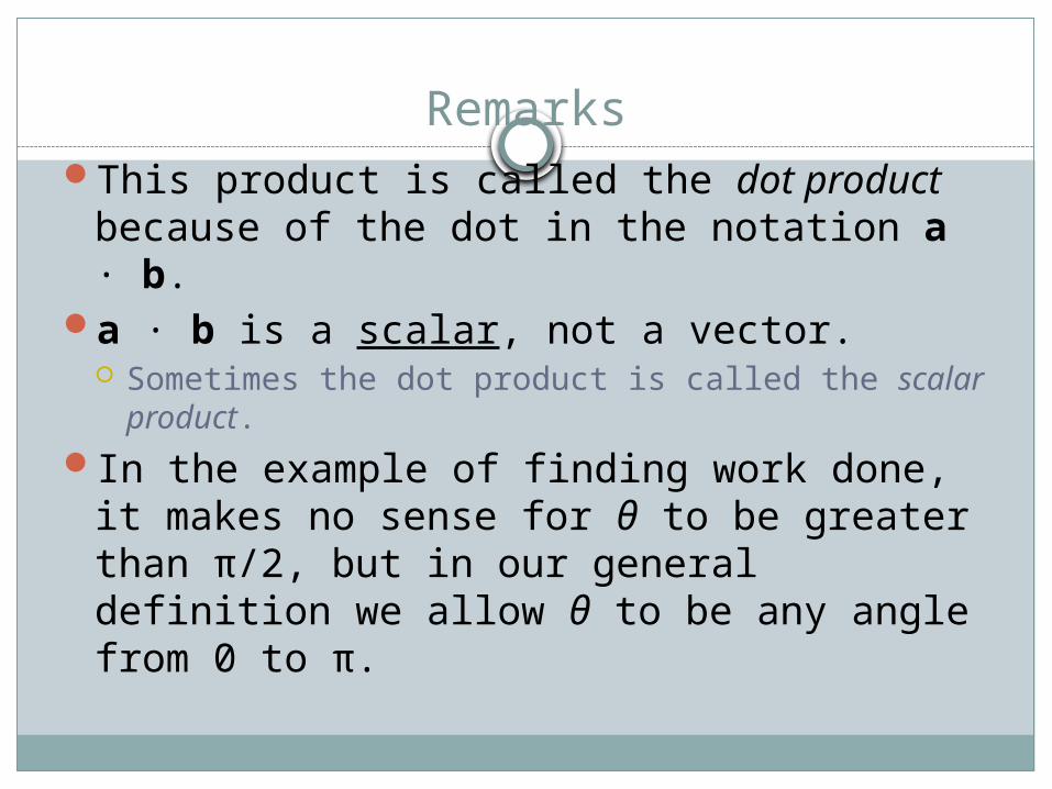
RemarksThis product is called the dot product
because of the dot in the notation a ∙ b.a ∙ b is a scalar, not a vector. Sometimes the dot product is called the scalar
product.In the example of finding work done, it
makes no sense for θ to be greater than π/2, but in our general definition we allow θ to be any angle from 0 to π.
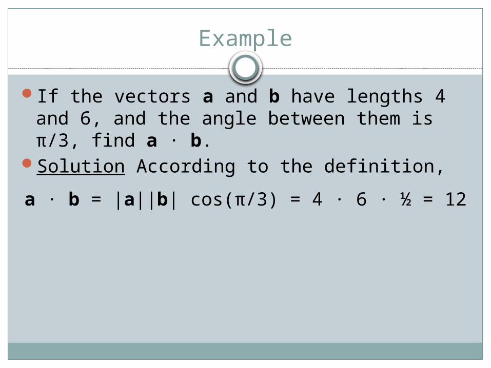
Example
If the vectors a and b have lengths 4 and 6, and the angle between them is π/3, find a ∙ b.
Solution According to the definition,
a ∙ b = |a||b| cos(π/3) = 4 ∙ 6 ∙ ½ = 12

Perpendicular Vectors
Two nonzero vectors a and b are called perpendicular or orthogonal if the angle between them is θ = π/2.
For such vectors we have
a ∙ b = |a||b| cos(π/2) = 0Conversely, if a ∙ b = 0, then cos θ = 0, so
θ = π/2.

Perpendicular Vectors (cont’d)Since the zero vector 0 is considered to be
perpendicular to all vectors, we have
Further, by properties of the cosine, a ∙ b is positive for θ < π/2, and negative for θ > π/2,
as the next slide illustrates:

Perpendicular Vectors (cont’d)

Perpendicular Vectors (cont’d)We can think of a ∙ b as measuring the
extent to which a and b point in the same general direction.
The dot product a ∙ b is… positive if a and b point in the same general
direction, 0 if they are perpendicular, and negative if they point in generally opposite
directions.

Example
Find the angle between
Solution Let θ be the required angle. Since
2,2, 1 anda 5, 3,2 .b
22 2
22 2
2 2 1 3 and
5 3 2 38
a
b
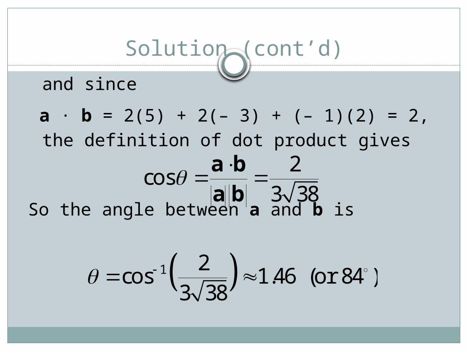
Solution (cont’d)
and since
a ∙ b = 2(5) + 2(– 3) + (– 1)(2) = 2,the definition of dot product gives
So the angle between a and b is
2cos
3 38a ba b
1 2cos 1.46 (or 84 )
3 38

Vectors
Length and direction. Absolute position not important
Use to store offsets, displacements, locations But strictly speaking, positions are not vectors and cannot
be added: a location implicitly involves an origin, while an offset does not.
=
Usually written as or in bold. Magnitude written as a a

Vector Addition
Geometrically: Parallelogram ruleIn cartesian coordinates (next), simply add coords
a
ba+b = b+a

Cartesian Coordinates
X and Y can be any (usually orthogonal unit) vectors
X
A = 4 X + 3 Y
2 2 TxA A x y A x y
y

Vector Multiplication
Dot product Cross product Orthonormal bases

Dot (scalar) product
a
b
?a b b a
1
cos
cos
a b a b
a b
a b
( )
( ) ( ) ( )
a b c a b a c
ka b a kb k a b

Dot product: some applications
Find angle between two vectors (e.g. cosine of angle between light source and surface for shading)
Finding projection of one vector on another (e.g. coordinates of point in arbitrary coordinate system)
Advantage: can be computed easily in cartesian components

Projections (of b on a)
a
b
?
?
b a
b a
cosa b
b a ba
2
a a bb a b a a
a a

Dot product in Cartesian components
?a b
a b
x xa b
y y
a ba b a b
a b
x xa b x x y y
y y

What is a matrix
Array of numbers (m×n = m rows, n columns)
Addition, multiplication by a scalar simple: element by element
1 3
5 2
0 4

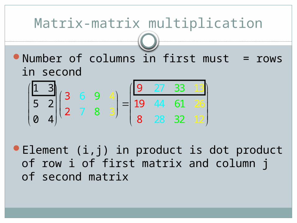
Matrix-matrix multiplication
Number of columns in first must = rows in second
Element (i,j) in product is dot product of row i of first matrix and column j of second matrix
1 33 6 9 4
5 22 7 8 3
0 4
Matrix-matrix multiplication
Number of columns in first must = rows in second
Element (i,j) in product is dot product of row i of first matrix and column j of second matrix
9 21 3 7 3
5 2
0 4
1339
618
3
319
28 2
426
3
644
17
28 2

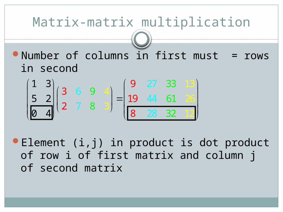
Matrix-matrix multiplication
Number of columns in first must = rows in second
Element (i,j) in product is dot product of row i of first matrix and column j of second matrix
9 21 3 7 3
5 2
0 4
1339
618
3
319
28 2
426
3
644
17
28 2
Matrix-matrix multiplication
Number of columns in first must = rows in second
Element (i,j) in product is dot product of row i of first matrix and column j of second matrix
9 21 3 7 3
5 2
0 4
1339
618
3
319
28 2
426
3
644
17
28 2

Matrix-matrix multiplication
Number of columns in first must = rows in second
Non-commutative (AB and BA are different in general)
Associative and distributive A(B+C) = AB + AC (A+B)C = AC + BC
1 33 6 9 4
5 2 NOT EVEN LEGAL!!2 7 8 3
0 4

Matrix-Vector Multiplication
1 0
0 1
x x
y y

Transpose of a Matrix (or vector?)
1 21 3 5
3 42 4 6
5 6
T
( )T T TAB B A

Identity Matrix and Inverses
1 1
1 1 1( )
AA A A I
AB B A
3 3
1 0 0
0 1 0
0 0 1
I
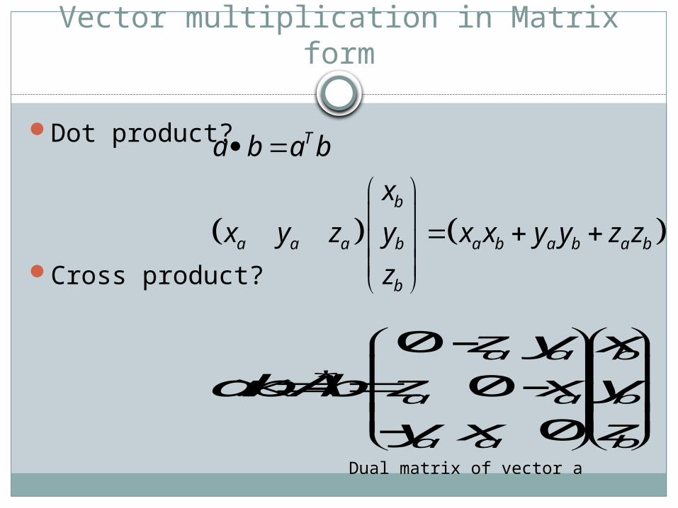
Vector multiplication in Matrix form
Dot product?
Cross product?
T
b
a a a b a b a b a b
b
a b a b
x
x y z y x x y y z z
z
*
0
0
0
a a b
a a b
a a b
z y x
a b A b z x y
y x z
Dual matrix of vector a

Vector basis
A set of vectors (v1, ..., vk) is said to be a basis for a vector space W if
(1) (v1, ..., vk) are linearly independent
(2) (v1, ..., vk) span W
Standard bases:R2 R3 Rn
Determinants

Determinant - a square array of numbers or variables enclosed between parallel vertical bars.
**To find a determinant you must have a SQUARE MATRIX!!**
a b = ad - bc
c d
Finding a 2 x 2 determinant:

Find the determinant:
1. 5 7
11 8 5 8 7 11 40 77
37 40 77
2. 3 2
1 5 3 5 2 1 15 2
1715 2
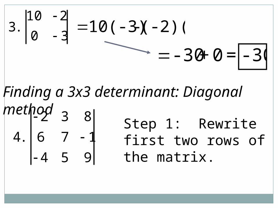
3. 10 20 3
10(-3) - (-2)(0)
-30 + 0 = -30
Finding a 3x3 determinant: Diagonal method
4.
2 3 8
6 7 1
4 5 9
Step 1: Rewrite first two rows of the matrix.

4.
2 3 8
6 7 1
4 5 9
2 3
6 7
4 5
Step 2: multiply diagonals going up!
-224+10
+162
= -52
Step 2: multiply diagonals going down!
-126
+12+240
=126
Step 3: Bottom minus top!
126 - (-52)
126 + 52
= 178

5.
5 1 2
2 3 5
3 2 3
Step 2: multiply diagonals going up!
-18+50
+6= 38
Step 2: multiply diagonals going down!
45- 15+ 8 = 38
Step 3: Bottom minus top!
38 - 38
= 0
5 1
2 33 2

5.2 Expansion by CofactorsDefinition 1: Given a matrix A, a minor is the determinant of any square submatrix of A.
Definition 2: Given a matrix A=[aij] , the cofactor of the element aij is a scalar obtained by multiplying together the term (-1)i+j and the minor obtained from A by removing the ith row and the jth column.
In other words, the cofactor Cij is given by Cij = (1)i+jMij.
For example,
333231
232221
131211
aaa
aaa
aaa
A 3332
131221 aa
aaM
3331
131122 aa
aaM
212112
21 )1( MMC
222222
22 )1( MMC
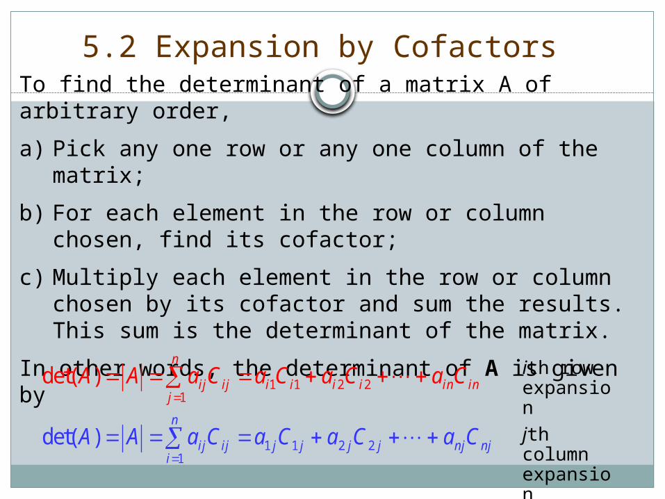
5.2 Expansion by CofactorsTo find the determinant of a matrix A of arbitrary order,
a) Pick any one row or any one column of the matrix;
b) For each element in the row or column chosen, find its cofactor;
c) Multiply each element in the row or column chosen by its cofactor and sum the results. This sum is the determinant of the matrix.
In other words, the determinant of A is given by
ininiiii
n
jijij CaCaCaCaAA
2211
1
)det(
njnjjjjj
n
iijij CaCaCaCaAA
2211
1
)det(
ith row expansion
jth column expansion

Example 1:We can compute the determinant
1 2 3
4 5 6
7 8 9
T
by expanding along the first row,
1 1 1 2 1 35 6 4 6 4 51 2 3
8 9 7 9 7 8 T 3 12 9 0
Or expand down the second column:
1 2 2 2 3 24 6 1 3 1 32 5 8
7 9 7 9 4 6 T 12 60 48 0
Example 2: (using a row or column with many zeroes)
2 3
1 5 01 5
2 1 1 13 1
3 1 0
16

5.3 Properties of determinantsProperty 1: If one row of a matrix consists entirely of zeros, then the determinant is zero.
Property 2: If two rows of a matrix are interchanged, the determinant changes sign.
Property 3: If two rows of a matrix are identical, the determinant is zero.
Property 4: If the matrix B is obtained from the matrix A by multiplying every element in one row of A by the scalar λ, then |B|= λ|A|.
Property 5: For an n n matrix A and any scalar λ, det(λA)= λndet(A).

5.3 Properties of determinants
Property 6: If a matrix B is obtained from a matrix A by adding to one row of A, a scalar times another row of A, then |A|=|B|.
Property 7: det(A) = det(AT).
Property 8: The determinant of a triangular matrix, either upper or lower, is the product of the elements on the main diagonal.
Property 9: If A and B are of the same order, then det(AB)=det(A)
det(B).

5.5 Inversion
Theorem 1: A square matrix has an inverse if and only if its determinant is not zero.
Below we develop a method to calculate the inverse of nonsingular matrices using determinants.
Definition 1: The cofactor matrix associated with an n n matrix A is an n n matrix Ac obtained from A by replacing each element of A by its cofactor.
Definition 2: The adjugate of an n n matrix A is the transpose of the cofactor matrix of A: Aa = (Ac)T

Inversion using determinants
Theorem 2: A Aa = Aa A = |A| I .
If |A| ≠ 0 then from Theorem 2,
011
AifAA
A
IAA
A
A
AA
a
aa
That is, if |A| ≠ 0, then A-1 may be obtained by dividing the adjugate of A by the determinant of A.
For example, if
then
,
dc
baA
ac
bd
bcadA
AA a 111

Find the adjugate of
Solution:The cofactor matrix of A:
201
120
231
A
20
31
10
21
12
2301
31
21
21
20
2301
20
21
10
20
12
217
306
214
232
101
764aA
Example of finding adjugate
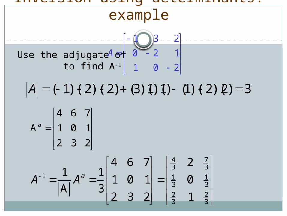
Use the adjugate of to find A-1
201
120
231
A
232
101
764
Aa
3)2)(2)(1()1)(1)(3()2)(2)(1( A
32
32
31
31
37
34
1
1
0
2
232
101
764
3
1
A
1 aAA
Inversion using determinants: example

Matrix Operations
Matrix addition/subtraction Matrices must be of same size.
Matrix multiplication
Condition: n = q
m x n q x p m x p

Identity Matrix

Matrix Transpose

Symmetric Matrices
Example:

Determinants
2 x 2
3 x 3
n x n

Determinants (cont’d)
diagonal matrix:

Matrix Inverse
The inverse A-1 of a matrix A has the property:
AA-1=A-1A=I
A-1 exists only if
Terminology Singular matrix: A-1 does not exist Ill-conditioned matrix: A is close to being
singular

Matrix Inverse (cont’d)
Properties of the inverse:

Pseudo-inverse
The pseudo-inverse A+ of a matrix A (could be non-square, e.g., m x n) is given by:
It can be shown that:

Orthonormal matrices
• A is orthonormal if:
• Note that if A is orthonormal, it easy to find its inverse:
Property:

Matrix trace
properties:

Rank of matrix
Equal to the dimension of the largest square sub-matrix of A that has a non-zero determinant.
Example: has rank 3
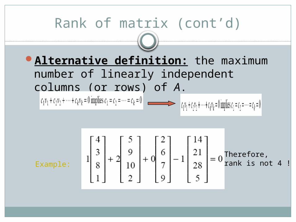
Rank of matrix (cont’d)
Alternative definition: the maximum number of linearly independent columns (or rows) of A.
Therefore,rank is not 4 !Example:

Rank and singular matrices

Review on “rank”
“row-rank of a matrix” counts the max. number of linearly independent rows.
“column-rank of a matrix” counts the max. number of linearly independent columns.
One application: Given a large system of linear equations, count the number of essentially different equations. The number of essentially different equations is just
the row-rank of the augmented matrix.
kshumENGG2013
67
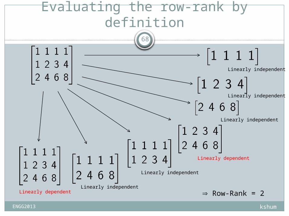
Evaluating the row-rank by definition
kshumENGG2013
68
Linearly independent
Linearly independent
Linearly independent
Linearly independent
Linearly independent
Linearly dependent
Linearly dependent Row-Rank = 2

Calculation of row-rank via RREF
kshumENGG2013
69
Row reductions
Row-rank = 2Row-rank = 2
Because row reductionsdo not affect the numberof linearly independent rows

Calculation of column-rank by definition
kshumENGG2013
70
List all combinationsof columns
Linearly independent??
Y Y Y Y Y Y Y Y Y
N N
Y
N N
N
Column-Rank = 2

Theorem
Given any matrix, its row-rank and column-rank are equal.
In view of this property, we can just say the “rank of a matrix”. It means either the row-rank of column-rank.
kshumENGG2013
71

Why row-rank = column-rank?
If some column vectors are linearly dependent, they remain linearly dependent after any elementary row operation
For example, are linearly dependent
kshumENGG2013
72

Why row-rank = column-rank?
Any row operation does not change the column- rank.
By the same argument, apply to the transpose of the matrix, we conclude that any column operation does not change the row-rank as well.
kshumENGG2013
73

Why row-rank = column-rank?
kshumENGG2013
74
Apply row reductions.row-rank and column-rankdo not change.
Apply column reductions.row-rank and column-rankdo not change.
The top-left corner isan identity matrix.
The row-rank and column-rank of this “normal form” is certainlythe size of this identity submatrix,and are therefore equal.

If a system of n linear equations in n variables Ax=b has a coefficient matrix with a nonzero determinant |A|,then the solution of the system is given by
where Ai is a matrix obtained from A by replacing the ith column of A by the vector b.
Example:
,)det(
)det(,,
)det(
)det(,
)det(
)det( 22
11 A
Ax
A
Ax
A
Ax n
n
3333232131
2323222121
1313212111
bxaxaxa
bxaxaxa
bxaxaxa
333231
232221
131211
33231
22221
112113
3
aaa
aaa
aaa
baa
baa
baa
A
Ax
5.6 Cramer’s rule

Use Cramer’s Rule to solve the system of linear equation.
2443
02
132
zyx
zx
zyx
10
443
102
321
A
10
442
100
321
1
A
Ax
5
4
10
8
10
)1)(1)(4()2)(1)(2(
5
8,
2
3 zy
5.6 Cramer’s rule: example

Copyright © by Houghton Mifflin Company, Inc. All rights reserved.
77
A solution of such a system is an ordered pair which is a solution of each equation in the system.
Example: The ordered pair (4, 1) is a solution of the system since
3(4) + 2(1) = 14 and 2(4) – 5(1) = 3.
A set of linear equations in two variables is called a system of linear equations.
3x + 2y = 14
2x + 5y = 3
Example: The ordered pair (0, 7) is not a solution of the system
since
3(0) + 2(7) = 14 but 2(0) – 5(7) = – 35, not 3.

Copyright © by Houghton Mifflin Company, Inc. All rights reserved.
78
A system of equations with at least one solution is consistent. A system with no solutions is inconsistent.
Systems of linear equations in two variables have either no solutions, one solution, or infinitely many solutions.
y
x
infinitely many solutions
y
x
no solutions
y
x
unique solution

Copyright © by Houghton Mifflin Company, Inc. All rights reserved.
79
The ordered pair (1, 2) is the unique solution.
The system is consistent since it has solutions.
y
xx – y = –1
2x + y = 4
(1, 2)
To solve the system by the graphing
method, graph both equations and determine where the
graphs intersect.
x – y = –12x + y = 4

Copyright © by Houghton Mifflin Company, Inc. All rights reserved.
80
The system has no solutions and is inconsistent.The lines are parallel and have no point of intersection.
y
x
x – 2y = – 4
3x – 6y = 6
Example: Solve the system by the
graphing method.
x – 2y = – 4
3x – 6y = 6

Copyright © by Houghton Mifflin Company, Inc. All rights reserved.
81
The graphs of the two equations are the same line and the intersection points are all the points on this line.
The system has infinitely many solutions.
y
x
x – 2y = – 43x – 6y = – 12
Example: Solve the system by the graphing
method.
x – 2y = – 43x – 6y = – 12

Copyright © by Houghton Mifflin Company, Inc. All rights reserved.
82
1. From the second equation obtain x = 3y – 3.
3. Solve for y to obtain y = 2.
4. Substitute 2 for y in x = 3y – 3 and conclude x = 3. The solution is (3, 2).
2. Substitute this expression for x into the first equation.
2(3y –3) + y = 8
5. Check:2(3) – (2) = 8
(3) – 3(2) = –3
Example: Solve the system by the substitution
method.
2x + y = 8x – 3y = – 3
Copyright © by Houghton Mifflin Company, Inc. All rights reserved.
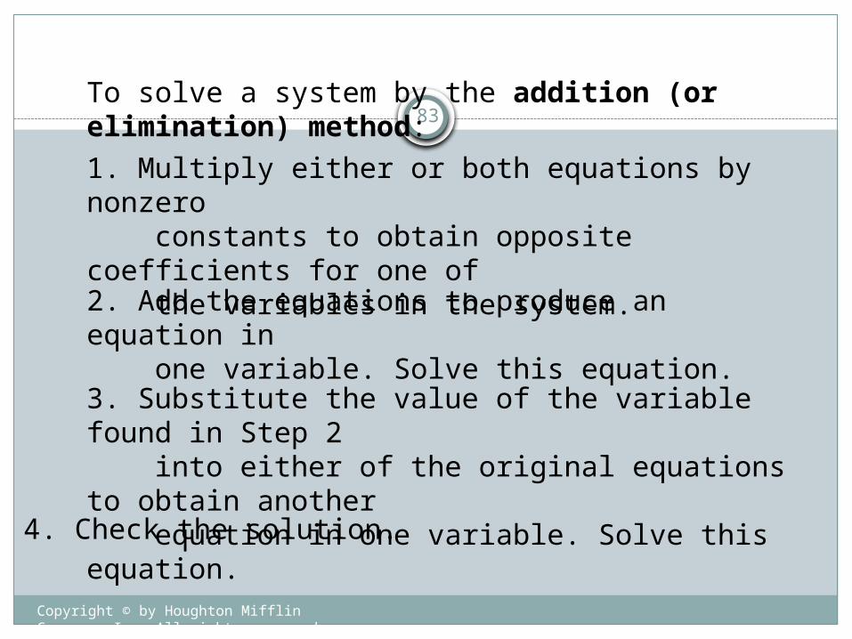
83To solve a system by the addition (or elimination) method:
1. Multiply either or both equations by nonzero constants to obtain opposite coefficients for one of the variables in the system.
2. Add the equations to produce an equation in one variable. Solve this equation.
3. Substitute the value of the variable found in Step 2 into either of the original equations to obtain another equation in one variable. Solve this equation.
4. Check the solution.

Copyright © by Houghton Mifflin Company, Inc. All rights reserved.
84
1. From the first equation obtain y = 2x – 10.
2. Substitute 2x – 10 for y into the second equation to produce 4x – 2(2x – 10) = 8.
3. Attempt to solve for x.4x – 2(2x – 10) = 84x – 4x + 20 = 820 = 8 False statement
Because there are no values of x and y for which 20 equals 8, this system has no solutions.
Example: Solve the system by the substitution method.
2x – y = 104x – 2y = 8

Copyright © by Houghton Mifflin Company, Inc. All rights reserved.
85
System discussion and solving
SCD if R(A)=R(A’)=nº eq.(1 solution)
SCI if R(A)=R(A’)<nº eq.(∞ solutions)
SI if R(A)≠R(A’) (no solution)

Eigenvalues and Eigenvectors
The vector v is an eigenvector of matrix A and λ is an eigenvalue of A if:
Interpretation: the linear transformation implied by A cannot change the direction of the eigenvectors v, only their magnitude.
(assume non-zero v)

Computing λ and v
To find the eigenvalues λ of a matrix A, find the roots of the characteristic polynomial:
Example:
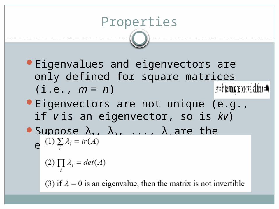
Properties
Eigenvalues and eigenvectors are only defined for square matrices (i.e., m = n)
Eigenvectors are not unique (e.g., if v is an eigenvector, so is kv)
Suppose λ1, λ2, ..., λn are the eigenvalues of A, then:

Properties (cont’d)
xTAx > 0 for every

Matrix diagonalization
Given A, find P such that P-1AP is diagonal (i.e., P diagonalizes A)
Take P = [v1 v2 . . . vn], where v1,v2 ,. . . vn are
the eigenvectors of A:
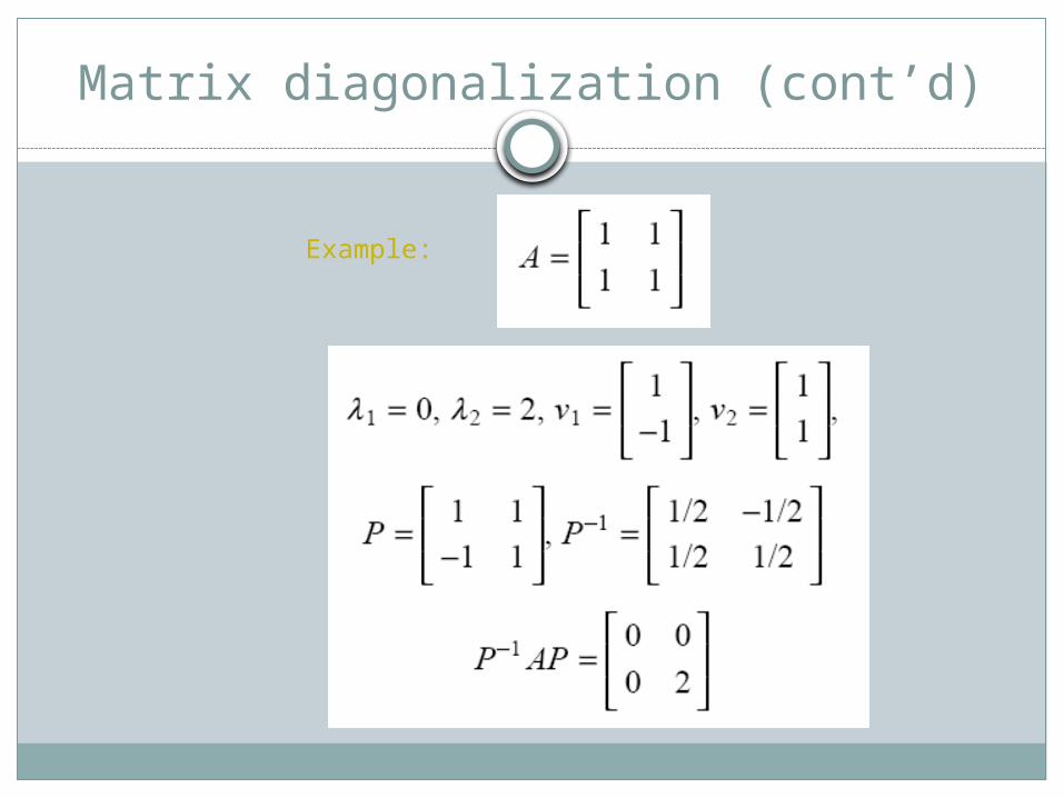
Matrix diagonalization (cont’d)
Example:
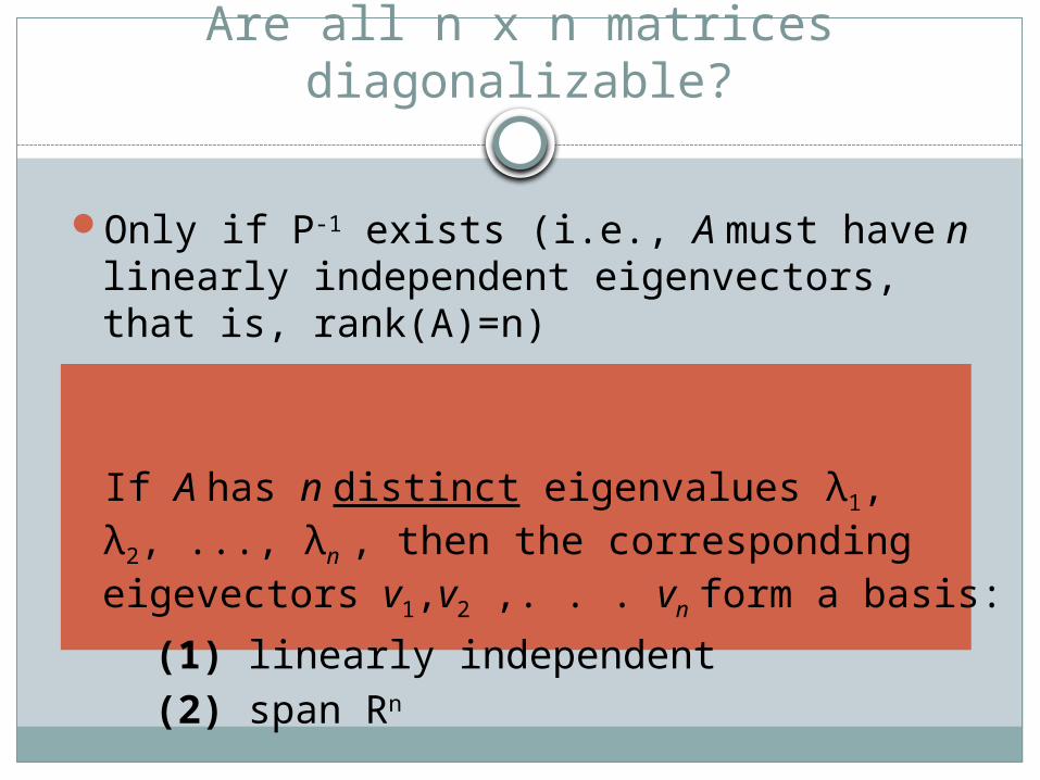
Only if P-1 exists (i.e., A must have n linearly independent eigenvectors, that is, rank(A)=n)
If A has n distinct eigenvalues λ1, λ2, ..., λn , then the corresponding eigevectors v1,v2 ,. . . vn form a basis:
(1) linearly independent (2) span Rn
Are all n x n matrices diagonalizable?

Diagonalization Decomposition
Let us assume that A is diagonalizable, then:

Decomposition: symmetric matrices
• The eigenvalues of symmetric matrices are all real.
• The eigenvectors corresponding to distinct eigenvalues are orthogonal.
A=PDPT=
P-1=PT

Domain and RangeFunctions have an independent variable (often x) and a dependent variable (often y).
In this discussion we are going to use x for the independent variable and y for the dependent variable, but we could use other letters.
domain: The set of all possible x values for a function.
range: The set of all possible y values for a function.
We can specify the domain of a function, or we can look at the nature of the function to determine the natural domain of the function.

Example:
Find the domain and range of: 1f x
x
When finding the domain, it is often easier to think of what values that we cannot use for x.
In this case, x cannot equal zero. The domain is:
,0 0,D or 0D x x
We usually use interval notation.
These are open intervals (with parentheses) because we don’t count the zero. Also notice the symbol for union.
This is set builder notation.

1f x
x
Looking at the graph, we see that we can have every y value except zero, so the range is:
,0 0,D or 0D x x
x
y
x
y
,0 0,R

Another example:
Find the domain and range of: y x
Since we cannot take the square root of a negative number, the domain is:
This is a half-open interval.
We use a square bracket on the left boundary point because we count the zero. (The interval is closed at zero.)
When infinity is a boundary, it is always an open interval on that end, with parentheses.
[0, )D

x
y
Looking at the graph, we see that there are no negative y values, so the range is:
0,R
Another example:
Find the domain and range of: y x
Since we cannot take the square root of a negative number, the domain is: [0, )D

x
y
x
y
x
y
SymmetryWhen we graph the function , we see that it hasy-axis symmetry.
2y x
When we square the x, any negative sign cancels out, so changing the sign of x does not change the y value.
Any polynomial function with only even exponents behaves the same way, and has y-axis symmetry.
4 22 1y x x
This is , which has an even exponent. 0x

x
y
x
y
Any function with y-axis symmetry is called an even function.
For example, is an even function.y x
So is . cosy x
x
y
x
y
x
y
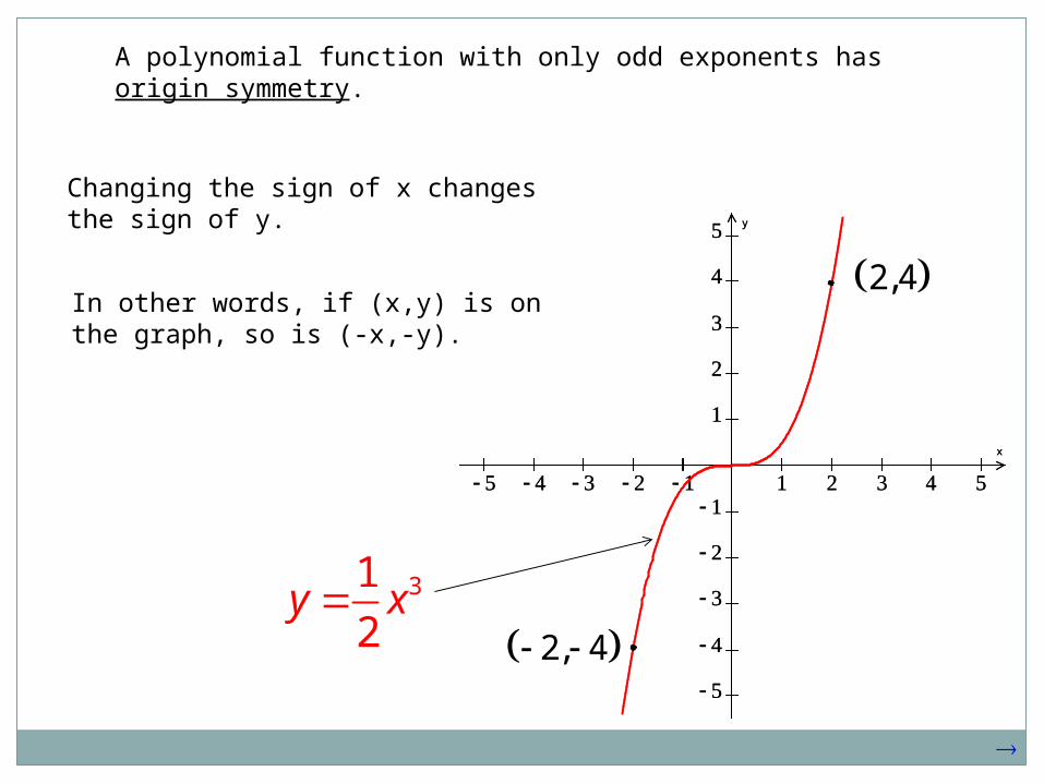
A polynomial function with only odd exponents hasorigin symmetry.
Changing the sign of x changes the sign of y.
31
2y x
In other words, if (x,y) is on the graph, so is (-x,-y).
2,4
2, 4
x
y
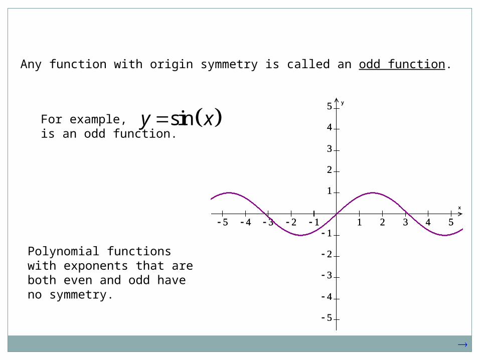
Any function with origin symmetry is called an odd function.
For example, is an odd function.
siny x
x
y
Polynomial functions with exponents that are both even and odd have no symmetry.

x
y
Of course, a graph with x-axis symmetry is not a function at all!
x
y
x y
Fails the vertical line test!

x
y
Piecewise FunctionsWhile many functions can be defined by a single formula, others are
defined by applying different formulas to different parts of their domains.
Just graph each piece separately, for each part of the domain.
Example:
2
, 0
, 0 1
1, 1
x x
y f x x x
x

x
y
Write a piecewise function for the graph at right:
Example:
There are two pieces to this graph, so we need two equations.
1,1 2,1
, 0 1
1, 1 2
x xf x
x x
The equation for the left hand piece is: y xFor the right hand piece, the equation is: 0 1 1y x
This simplifies to: 1y x
Paying attention to the open and closed circles, we get the piecewise function:
p

Limits and Continuity
•Definition•Evaluation of Limits•Continuity
•Limits Involving Infinity

Limit
We say that the limit of ( ) as approaches is and writef x x a L
lim ( ) x a
f x L
if the values of ( ) approach as approaches . f x L x a
a
L( )y f x

Limits, Graphs, and Calculators
21
11. a) Use table of values to guess the value of lim
1x
x
x
2
1b) Use your calculator to draw the graph ( )
1
xf x
x
and confirm your guess in a)
2. Find the following limits
0
sina) lim by considering the values
x
x
x
1, 0.5, 0.1, 0.05, 0.001. x Thus the limit is 1. sin
Confirm this by ploting the graph of ( ) x
f xx
Graph 1
Graph 2

0
b) limsin by considering the values x x
p
1 1 1(i) 1, , , 10 100 1000x
2 2 2(ii) 1, , , 3 103 1003x
This shows the limit does not exist.
Confrim this by ploting the graph of ( ) sin f x xp
Graph 3
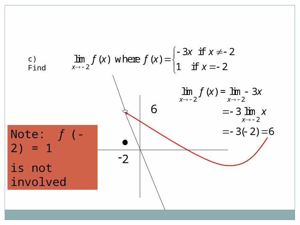
c) Find2
3 if 2lim ( ) where ( )
1 if 2x
x xf x f x
x
-2
62 2
lim ( ) = lim 3x x
f x x
Note: f (-2) = 1
is not involved
23 lim
3( 2) 6x
x

2
2
4( 4)a. lim
2x
x
x
0
1, if 0b. lim ( ), where ( )
1, if 0x
xg x g x
x
20
1c. lim ( ), where f ( )
xf x x
x
0
1 1d. lim
x
x
x
Answer : 16
Answer : no limit
Answer : no limit
Answer : 1/2
3) Use your calculator to evaluate the limits

The Definition of Limit-
lim ( ) We say if and only if x a
f x L
given a positive number , there exists a positive such that
if 0 | | , then | ( ) | . x a f x L
( )y f x a
LL
L
a a

such that for all in ( , ), x a a a
then we can find a (small) interval ( , )a a
( ) is in ( , ).f x L L
This means that if we are given a
small interval ( , ) centered at , L L L
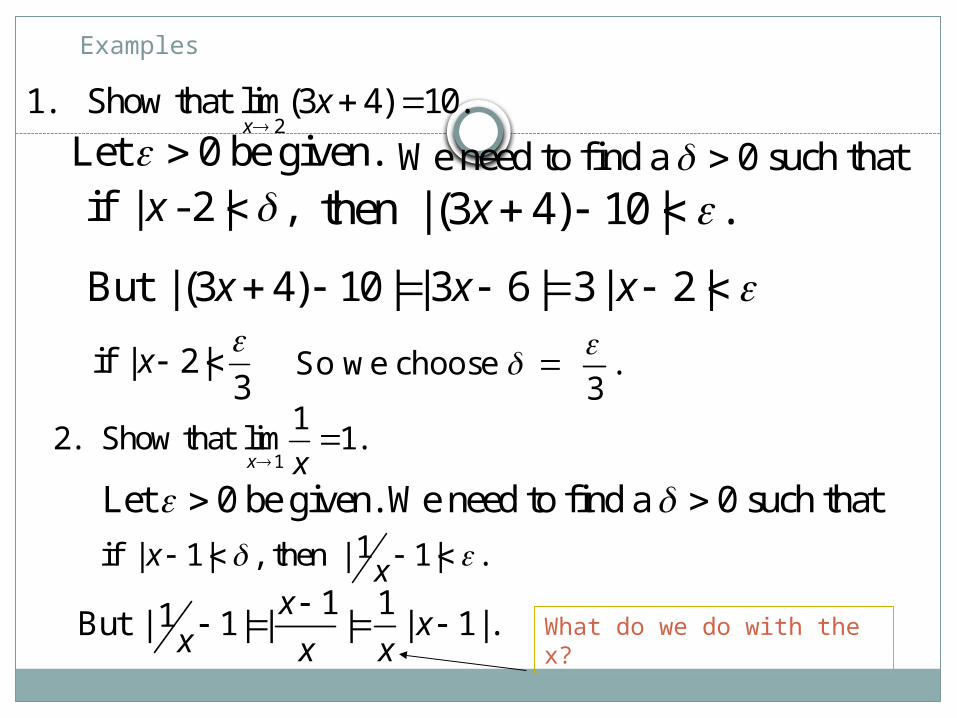
Examples
21. Show that lim(3 4) 10.
xx
Let 0 be given. We need to find a 0 such that if | - 2 | ,x then | (3 4) 10 | .x
But | (3 4) 10 | | 3 6 | 3 | 2 |x x x
if | 2 |3
x
So we choose .3
1
12. Show that lim 1.
x x
Let 0 be given. We need to find a 0 such that 1if | 1| , then | 1| .x x
1 11But | 1| | | | 1| . x
xx x x
What do we do with the x?

1 31If we decide | 1| , then . 2 22x x
1And so <2.
x
1/2
11Thus | 1| | 1| 2 | 1| . x xx x
1 Now we choose min , .
3 2
1 3/2

The right-hand limit of f (x), as x approaches a, equals L
written:
if we can make the value f (x) arbitrarily close to L by taking x to be sufficiently close to the right of a.
lim ( )x a
f x L
a
L( )y f x
One-Sided Limit One-Sided Limits

The left-hand limit of f (x), as x approaches a, equals M
written:
if we can make the value f (x) arbitrarily close to L by taking x to be sufficiently close to the left of a.
lim ( )x a
f x M
a
M
( )y f x

2 if 3( )
2 if 3
x xf x
x x
1. Given
3lim ( )x
f x
3 3lim ( ) lim 2 6x x
f x x
2
3 3lim ( ) lim 9x x
f x x
Find
Find 3
lim ( )x
f x
Examples Examples of One-Sided Limit

1, if 02. Let ( )
1, if 0.
x xf x
x x
Find the limits:
0lim ( 1)x
x
0 1 1 0
a) lim ( )x
f x
0b) lim ( )
xf x
0lim( 1)x
x
0 1 1
1c) lim ( )
xf x
1lim( 1)x
x
1 1 2
1d) lim ( )
xf x
1lim( 1)x
x
1 1 2
More Examples

lim ( ) if and only if lim ( ) and lim ( ) .x a x a x a
f x L f x L f x L
For the function
1 1 1lim ( ) 2 because lim ( ) 2 and lim ( ) 2.x x x
f x f x f x
Bu
t
0 0 0lim ( ) does not exist because lim ( ) 1 and lim ( ) 1.x x x
f x f x f x
1, if 0( )
1, if 0.
x xf x
x x
This theorem is used to show a limit does not exist.
A Theorem

Limit Theorems
If is any number, lim ( ) and lim ( ) , thenx a x a
c f x L g x M
a) lim ( ) ( )x a
f x g x L M
b) lim ( ) ( ) x a
f x g x L M
c) lim ( ) ( )x a
f x g x L M
( )d) lim , ( 0)( )x a
f x L Mg x M
e) lim ( )x a
c f x c L
f) lim ( ) n n
x af x L
g) lim x a
c c
h) lim x a
x a
i) lim n n
x ax a
j) lim ( ) , ( 0)
x af x L L

Examples Using Limit RuleEx. 2
3lim 1x
x
2
3 3lim lim1x x
x
23 3
2
lim lim1
3 1 10
x xx
Ex.1
2 1lim
3 5x
x
x
1
1
lim 2 1
lim 3 5x
x
x
x
1 1
1 1
2lim lim1
3lim lim5x x
x x
x
x
2 1 1
3 5 8

More Examples
3 31. Suppose lim ( ) 4 and lim ( ) 2. Find
x xf x g x
3
a) lim ( ) ( ) x
f x g x
3 3 lim ( ) lim ( )
x xf x g x
4 ( 2) 2
3
b) lim ( ) ( ) x
f x g x
3 3 lim ( ) lim ( )
x xf x g x
4 ( 2) 6
3
2 ( ) ( )c) lim
( ) ( )x
f x g x
f x g x
3 3
3 3
lim 2 ( ) lim ( )
lim ( ) lim ( )x x
x x
f x g x
f x g x
2 4 ( 2) 5
4 ( 2) 4

Indeterminate forms occur when substitution in the limit results in 0/0. In such cases either factor or rationalize the expressions.
Ex.25
5lim
25x
x
x
Notice form0
0
5
5lim
5 5x
x
x x
Factor and cancel common factors
5
1 1lim
5 10x x
Indeterminate Forms

9
3a) lim
9x
x
x
9
( 3)
( 3)
( 3) = lim
( 9)x
x
x
x
x
9
9 lim
( 9)( 3)x
x
x x
9
1 1 lim
63x x
2
2 3 2
4b) lim
2x
x
x x
2 2
(2 )(2 )= lim
(2 )x
x x
x x
2 2
2 = lim
x
x
x
2
2 ( 2) 41
( 2) 4
More Examples

The Squeezing TheoremIf ( ) ( ) ( ) when is near , and if f x g x h x x a
, then lim ( ) lim ( )x a x a
f x h x L
lim ( ) x a
g x L
2
0 Show that liExampl m 0e: .
xx sin x
p
0
Note that we cannot use product rule because limx
sin xp
DNE! But 1 sin 1 xp 2 2 2and so sin . x x xx
p
2 2
0 0Since lim lim( ) 0,
x xx x
we use the Squeezing Theorem to conclude
2
0lim 0.x
x sin xp
See Graph

Continuity
A function f is continuous at the point x = a if the following are true:
) ( ) is definedi f a) lim ( ) exists
x aii f x
a
f(a)

A function f is continuous at the point x = a if the following are true:
) ( ) is definedi f a) lim ( ) exists
x aii f x
) lim ( ) ( )x a
iii f x f a
a
f(a)

At which value(s) of x is the given function discontinuous?
1. ( ) 2f x x 2
92. ( )
3
xg x
x
Continuous everywhere Continuous
everywhere except at 3x
( 3) is undefinedg
lim( 2) 2 x a
x a
and so lim ( ) ( )x a
f x f a
-4 -2 2 4
-2
2
4
6
-6 -4 -2 2 4
-10
-8
-6
-4
-2
2
4
Examples

2, if 13. ( )
1, if 1
x xh x
x
1lim ( )x
h x
an
d Thus h is not cont. at x=1.
11
lim ( )x
h x
3
h is continuous everywhere else
1, if 04. ( )
1, if 0
xF x
x
0lim ( )x
F x
1 and
0lim ( )x
F x
1
Thus F is not cont. at 0.x
F is continuous everywhere else
-2 2 4
-3
-2
-1
1
2
3
4
5
-10 -5 5 10
-3
-2
-1
1
2
3

Continuous Functions
A polynomial function y = P(x) is continuous at every point x.
A rational function is continuous at every point x in its domain.
( )( ) ( )p xR x q x
If f and g are continuous at x = a, then
, , and ( ) 0 are continuous
at
ff g fg g ag
x a

Intermediate Value Theorem
If f is a continuous function on a closed interval [a, b] and L is any number between f (a) and f (b), then there is at least one number c in [a, b] such that f(c) = L. ( )y f x
a b
f (a)
f (b)L
c
f (c) =

Example
2Given ( ) 3 2 5,
Show that ( ) 0 has a solution on 1,2 .
f x x x
f x
(1) 4 0
(2) 3 0
f
f
f (x) is continuous (polynomial) and since f (1) < 0 and f (2) > 0, by the Intermediate Value Theorem there exists a c on [1, 2] such that f (c) = 0.

Limits at Infinity
For all n > 0,1 1
lim lim 0n nx xx x
provided that is defined.
1nx
Ex.2
2
3 5 1lim
2 4x
x x
x
2
2
5 13lim
2 4x
x x
x
3 0 0 3
0 4 4
Divide by2x
2
2
5 1lim 3 lim lim
2lim lim 4
x x x
x x
x x
x

More Examples
3 2
3 2
2 3 21. lim
100 1x
x x
x x x
3 2
3 3 3
3 2
3 3 3 3
2 3 2
lim100 1x
x xx x x
x x xx x x x
3
2 3
3 22
lim1 100 1
1x
x x
x x x
22
1

0
2
3 2
4 5 212. lim
7 5 10 1x
x x
x x x
2
3 3 3
3 2
3 3 3 3
4 5 21
lim7 5 10 1x
x xx x x
x x xx x x x
2 3
2 3
4 5 21
lim5 10 1
7x
x x x
x x x
0
7
2 2 43. lim
12 31x
x x
x
2 2 4
lim12 31x
x xx x x
xx x
42
lim31
12x
xx
x
2
12

24. lim 1x
x x
22
2
1 1 lim
1 1x
x x x x
x x
2 2
2
1lim
1x
x x
x x
2
1 lim
1x x x
1 1
0

Infinite LimitsFor all n > 0,
1
limnx a x a
1
lim if is evennx a
nx a
1
lim if is oddnx a
nx a
-8 -6 -4 -2 2
-20
-15
-10
-5
5
10
15
20
-2 2 4 6
-20
-10
10
20
30
40
More Graphs
-8 -6 -4 -2 2
-20
-15
-10
-5
5
10
15
20

Examples
Find the limits2
20
3 2 11. lim
2x
x x
x
2
0
2 13= lim
2x
x x
3
2
3
2 12. lim
2 6x
x
x
3
2 1= lim
2( 3)x
x
x
-8 -6 -4 -2 2
-20
20
40

Limit and Trig Functions
From the graph of trigs functions
( ) sin and ( ) cosf x x g x x
we conclude that they are continuous everywhere
-10 -5 5 10
-1
-0.5
0.5
1
-10 -5 5 10
-1
-0.5
0.5
1
limsin sin and lim cos cosx c x c
x c x c

Tangent and Secant Tangent and secant are continuous everywhere in their domain, which is the set of all real numbers 3 5 7, , , , 2 2 2 2x p p p p
-6 -4 -2 2 4 6
-30
-20
-10
10
20
30
-6 -4 -2 2 4 6
-15
-10
-5
5
10
15
tany x
secy x

Examples
2
a) lim secx
xp
2
b) lim secx
xp
32
c) lim tanx
xp
3
2
d) lim tanx
xp
e) lim cotx
xp
32
g) lim cotx
xp
32
cos 0lim 0
sin 1x
x
xp
4
f) lim tanx
xp
1

Limit and Exponential Functions
-6 -4 -2 2 4 6
-2
2
4
6
8
10
, 1xy a a
-6 -4 -2 2 4 6
-2
2
4
6
8
10 , 0 1xy a a
The above graph confirm that exponential functions are continuous everywhere.lim x c
x ca a

Asymptotes
horizontal asymptotThe line is called a
of the curve ( ) if eihter
ey L
y f x
lim ( ) or lim ( ) .x x
f x L f x L
vertical asymptote The line is called a
of the curve ( ) if eihter
x c
y f x
lim ( ) or lim ( ) .x c x c
f x f x

ExamplesFind the asymptotes of the graphs of the functions2
2
11. ( )
1
xf x
x
1 (i) lim ( )
xf x
Therefore the line 1
is a vertical asymptote.
x
1.(iii) lim ( )x
f x
1(ii) lim ( )
xf x
.
Therefore the line 1
is a vertical asymptote.
x
Therefore the line 1
is a horizonatl asymptote.
y
-4 -2 2 4
-10
-7.5
-5
-2.5
2.5
5
7.5
10

2
12. ( )
1
xf x
x
21 1
1(i) lim ( ) lim
1x x
xf x
x
1 1
1 1 1= lim lim .
( 1)( 1) 1 2x x
x
x x x
Therefore the line 1
is a vertical asympNO t eT ot .
x
1(ii) lim ( ) .
xf x
Therefore the line 1
is a vertical asymptote.
x
(iii) lim ( ) 0.x
f x
Therefore the line 0
is a horizonatl asymptote.
y
-4 -2 2 4
-10
-7.5
-5
-2.5
2.5
5
7.5
10

(F) Continuity and Differentiability – Online Examples
Follow this link to One-sided derivatives from IES Software
And then follow this link to Investigating Differentiability of Piecewise Functions from D. Hill (Temple U.) and L. Roberts (Georgia College and State University
(G) Continuity and Differentiability
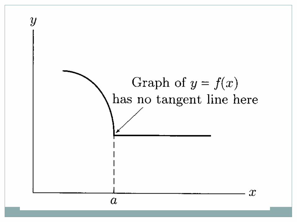
One other point to add that comes from our study of the last two examples even if a function is continuous, this does not always guarantee differentiability!!!!
If a continuous function as a cusp or a corner in it, then the function is not differentiable at that point see graphs on the next slide and decide how you would draw tangent lines (and secant lines for that matter) to the functions at the point of interest (consider drawing tangents/secants from the left side and from the right side)
As well, included on the graphs are the graphs of the derivatives (so you can make sense of the tangent/secant lines you visualized)


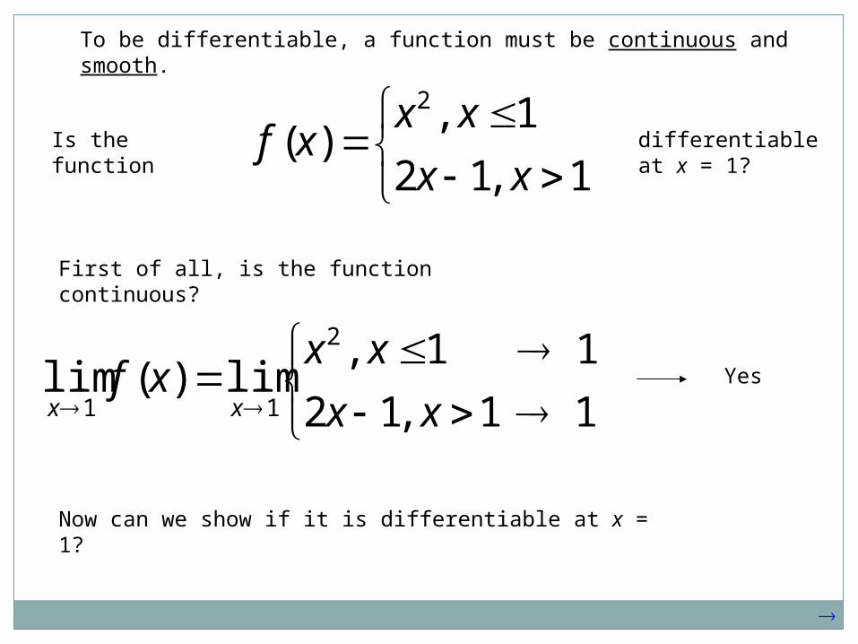
To be differentiable, a function must be continuous and smooth.
Derivatives will fail to exist at:
corner cusp
vertical tangent discontinuity
f x x 2
3f x x
3f x x 1, 0
1, 0
xf x
x

3.2 Differentiability
Greg Kelly, Hanford High School, Richland, WashingtonPhoto by Vickie Kelly, 2003
Arches National Park

To be differentiable, a function must be continuous and smooth.
Is the function continuous?
1,2
1,1)(
3
xx
xxxf
1lim)(lim 3
11
xxf
xx
xxfxx
2lim)(lim11
= 2
= 2
Answer: Yes

But by definition, what is a derivative?
h
xfhxfh
)(lim
0
A LIMIT
ax
afxfax
)(limor
This is another reason why we need to keep the definition of the derivative in mind before moving on to the short cuts for derivatives.

Is the function
1,2
1,1)(
3
xx
xxxf
)(lim1
xfx
= 3
But a limit only exists if it’s left and right limits are equal.
1
)1(lim
1 x
fxfx 1
21lim
3
1
x
xx
1
1lim
3
1 x
xx 1
)1)(1(lim
2
1
x
xxxx
3)(lim1
xfx
Differentiable at x = 1?
Differentiable also means that the left and right limits of the derivative are equal.

Differentiable also means that the left and right limits of the derivative are equal.
Is the function
1,2
1,1)(
3
xx
xxxf
)(lim1
xfx
= 2
Answer: No
1
)1(lim
1 x
fxfx 1
22lim
1
x
xx
1
)1(2lim
1
x
xx
2)(lim1
xfx
3)(lim1
xfx
≠
3)(lim1
xfx
Differentiable at x = 1?

To be differentiable, a function must be continuous and smooth.
Is the function Differentiable at x = 1?
1,2
1,1)(
3
xx
xxxf
Notice that on the left side, the slope is approaching 3
While on the right side, the slope is 2
2)(lim1
xfx
3)(lim1
xfx
≠
To be differentiable, a function must be continuous and smooth.
Is the function differentiable at x = 1?
1,12
1,)(
2
xx
xxxf
11,12
11,lim)(lim
2
11 xx
xxxf
xx
First of all, is the function continuous?
Yes
Now can we show if it is differentiable at x = 1?

To be differentiable, a function must be continuous and smooth.
Is the function differentiable at x = 1?
1,12
1,)(
2
xx
xxxf
1
1)(lim
2
1
x
xxf
x 1
)1)(1()(lim
1
x
xxxf
x
= 2
1
112)(lim
1
x
xxf
x 1
)1(2)(lim
1
x
xxf
x
= 2

To be differentiable, a function must be continuous and smooth.
Is the function differentiable at x = 1?
1,12
1,)(
2
xx
xxxf
Notice that on the left side, the slope is approaching 2
While on the right side, the slope is 2
Therefore, the answer is YES.

To be differentiable, a function must be continuous and smooth.
Derivatives will fail to exist at:
corner cusp
vertical tangent discontinuity
f x x 2
3f x x
3f x x 1, 0
1, 0
xf x
x

There are two theorems on page 110:
If f has a derivative at x = a, then f is continuous at x = a.
Since a function must be continuous to have a derivative, if it has a derivative then it is continuous.

Let a function have the derivative on a contiguous domain D(f '). Then is a function on D(f ') and, as such, may again have the derivative. If so, it is denoted
f x 'f x
'' ( )f x
'f x
and called the second derivative of f x
Sometimes we also use the denotation 2
2
d f x
dx
Examples
2
2
sin cossin
d x d xx
dx dx
22
21
nnd x
n n xd x

In a similar way, we can define the third, fourth, etc. derivative of a function if such derivatives exist. For a function we use the following notation f x
44
3( ), ,IV d f x
f x f xdx
33'''
3( ), ,
d f xf x f x
dx
,
nn
n
d f xf x
dx
the third derivative of f
the fourth derivative of f
the n-th derivative of f

If is defined on an interval and
f x ,a b
' 0 for f x a x b
then is increasing on ,a b f x
If
' 0 for f x a x b
f x ,a bthen is decreasing on
' 0f x
' 0f x

Bending-up and bending-down curves
Let be a continuous function defined on an interval f x ,a bAssume that exist for . We view the second derivative as the rate of change of the slope of the curve over the interval. If the second derivative is positive in the interval, then the slope of the curve is increasing and we interpret this as meanig that the curve is bending up. If the second derivative is negative, we interpret this as meaning that the curve is bending down.
' '' and f x f x a x b ''f x y f x
a b ba
'' 0f x '' 0f x
bending up bending down

Inflexion points
A point where a curve changes its behaviour from bending up to down (or vice versa) is called an inflexion point. If the curve is the graph of a function whose second derivative exists and is continuous, then we must have at that point. f x
'' 0f x
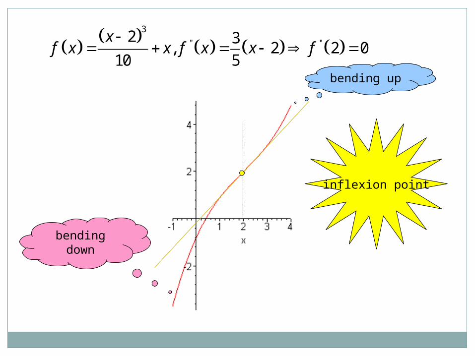
3
'' ''2 3, 2 2 0
10 5
xf x x f x x f
bending up
bending down
inflexion point

Maximum and local maximum of a function
Let a function be given with a domain . For a f x D f c D f
we say that c is the point of a maximum of the function if f x
:x D f f c f x
If a neigbourhood exists such that ,N c c
:x N f c f x
we say that has a local maximum at c. f x

Minimum and local minimum of a function
Let a function be given with a domain . For a f x D f c D f
we say that c is the point of a minimum of the function if f x
:x D f f c f x
If a neigbourhood exists such that ,N c c
:x N f c f x
we say that has a local minimum at c. f x

minimum
maximum
points of local maximum points of local minimum
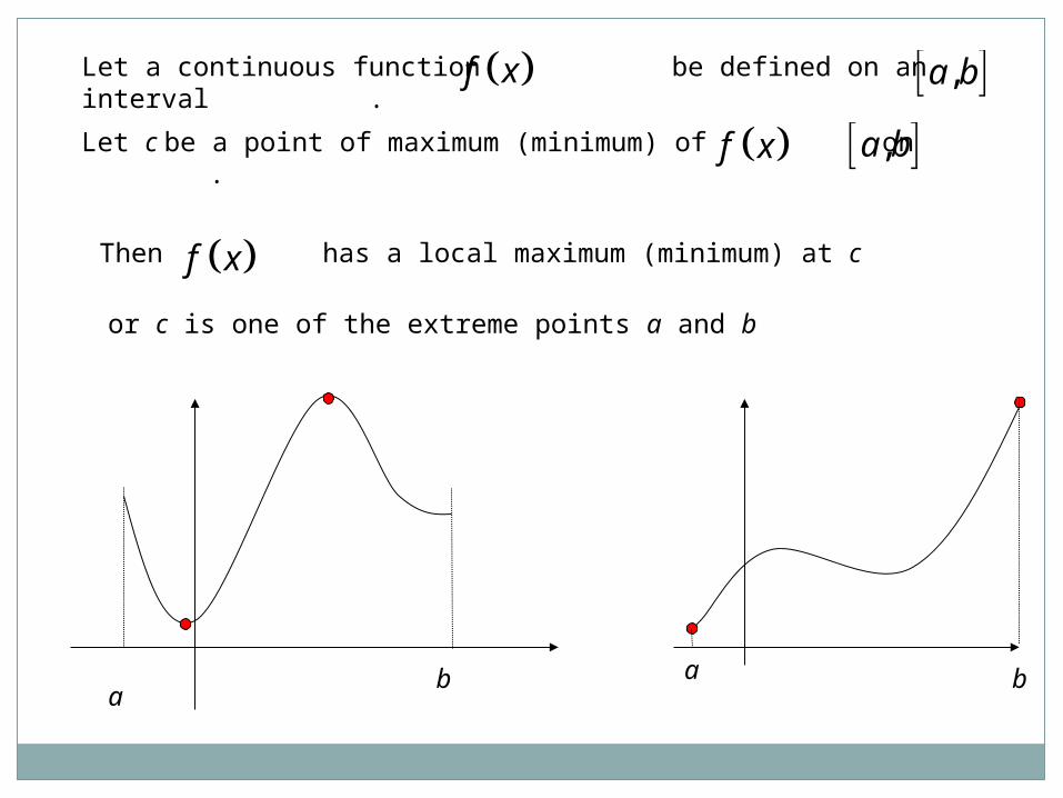
Let a continuous function be defined on an interval . f x ,a b
Let c be a point of maximum (minimum) of on .
f x
,a b
Then has a local maximum (minimum) at c
or c is one of the extreme points a and b
f x
ab a b

If a function is to have a local maximum at a point c, then there must be a neighbouhood of c such that �is increasing in and decreasing in
f x , ,c c c c
,c c f x ,c c
Thus we have
' 0 for , andf x x c c
' 0 for ,f x x c c
This is only possible if either of the derivative of at c does not exist.
' 0f c f x
For a local minimum, we may use a similar reasoning

A sufficient condition for a local minimum/maximum
If, for a function , we have
20, 1,2, , 2 1 0 for an integer 0i kf c i k f c k
f x
then has a local maximum at c. f x
If
then has a local minimum at c. f x
20, 1,2, , 2 1 0 for an integer 0i kf c i k f c k
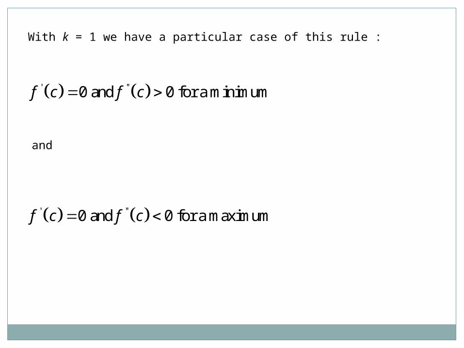
With k = 1 we have a particular case of this rule :
' ''0 and 0 for a minimumf c f c
and
' ''0 and 0 for a maximumf c f c

Example
Find minima and maxima of the function 3 22 3y x x
1' 333 3
2 2 22 3 2 1
3y x x
x x
3 1 0 1x x
4'' ''3
3
2 2 21
3 33y x y
x x
Maximum at -1.

Example
Verify if has a local maximum or minimum 4f x x
We have
4' 3 '' 2 '''( ) 4 , 12 , 24 , 24f x x f x x f x x f x
and so
4' '' '''0 0 0 0, 0 0f f f f
We conclude that f (x) has a local minimum at 0.

Example
Find the local minima and maxima of the function 1y x
x
y

We have
1 for 0
1 for 0
x x
y
x x
'
1 for 0
1 for 0
x
y
x
0
1 1lim 1
0x
x
x
0
1 1lim 1
0x
x
x
Thus at 0 does not exist which means that
0
1 1 0lim
0x
x
x
has no derivative at 0. Since it is increasing on the left of 0 and decreasing on the right, we conclude that it has a local maximum at 0.
1y x
Find the maxima and minima of the function on the interval [2, 1.5]
4 22y x x
' 34 4 4 1 1y x x x x x
Since local minima or maxima can only be reached at points
where the first derivative is zero and minima or maxima can also be reached at the extreme points, the only canidates for maxima and minima are the points 2,1,0,1,1.5. Calculating the values at these points we can verify that minima are reached at the points 1 and 1 while the maximum is reached at the point 2