
Olga V. Holtz UC Berkeley & TU Berlinoholtz/Talks/CS.pdf · An Introduction to Compressive Sensing...
27
An Introduction to Compressive Sensing Olga V. Holtz UC Berkeley & TU Berlin Stanford January 2009 History and Introduction Main idea Constructions Approximation theory
Transcript of Olga V. Holtz UC Berkeley & TU Berlinoholtz/Talks/CS.pdf · An Introduction to Compressive Sensing...

An Introduction to Compressive Sensing
Olga V. HoltzUC Berkeley & TU Berlin
StanfordJanuary 2009
History and Introduction Main idea Constructions Approximation theory

Compressed Sensing: History
Compressed Sensing (CS)
People involved, (Right to left: J. Claerbout, B. Logan, D. Donoho, E. Candés, T. Tao and R. DeVore)
History and Introduction Main idea Constructions Approximation theory

Compressed Sensing: Introduction
Old-fashioned Thinking
Collect data at grid points
For n pixels, take nobservations
Compressed Sensing (CS)
(CS camera at Rice)
Takes only O(n1/4 log5(n))random measurementsinstead of n
History and Introduction Main idea Constructions Approximation theory

Traditional signal processing
Model signals as band-limited functions x(t)
Support of x is contained in [−Ωπ,Ωπ]
Shannon-Nyquist
Uniform time sampling with spacing h ≤ 1/Ω gives exactreconstructon
A/D converters: sample and quantize
Problem: if Ω is very large, one cannot build circuits tosample at the desired rate
History and Introduction Main idea Constructions Approximation theory

Signal processing using CS
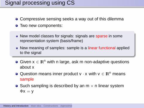
Compressive sensing seeks a way out of this dilemma
Two new components:
New model classes for signals: signals are sparse in somerepresentation system (basis/frame)
New meaning of samples: sample is a linear functional appliedto the signal
Given x ∈ IRn with n large, ask m non-adaptive questionsabout x
Question means inner product v · x with v ∈ IRn meanssample
Such sampling is described by an m × n linear systemΦx = y
History and Introduction Main idea Constructions Approximation theory
Signal processing using CS
Compressive sensing seeks a way out of this dilemma
Two new components:
New model classes for signals: signals are sparse in somerepresentation system (basis/frame)
New meaning of samples: sample is a linear functional appliedto the signal
Given x ∈ IRn with n large, ask m non-adaptive questionsabout x
Question means inner product v · x with v ∈ IRn meanssample
Such sampling is described by an m × n linear systemΦx = y
History and Introduction Main idea Constructions Approximation theory

Structure of signals
With no additional information on x cannot say anything
But we are interested in those x that have structure
Typically x can be represented by sparse linearcombinations of certain building blocks (e.g., a basis)
Issue: in many problems, we do not know the basis
Here we assume the basis is known (for now)
Ansatz: look for k -sparse solutions:
x ∈ Σk that is # supp(x) ≤ k .
History and Introduction Main idea Constructions Approximation theory

Sparsest Solutions of Linear equations
Find a sparsest solution of linear system
(P0) min‖x‖0 : Φx = b, x ∈ IRn
where ‖x‖0 = number of nonzeros of xand Φ ∈ IRm×n with m < n.
The solution is in generalnot unique.
Moreover, this problem isNP-Hard
History and Introduction Main idea Constructions Approximation theory

Basis Pursuit
Main idea:Use the convex relaxation
(P1) min‖x‖1 : Φx = b, x ∈ IRn
Basis Pursuit [Chen, Donoho, and Saunders (1999)]
Solving (P1) in polynomial time
Can be solved by linearprogramming:
min 1Ty
s.t.Φx = b−y ≤ x ≤ y
History and Introduction Main idea Constructions Approximation theory

Sparse Recovery and Mutual Incoherence
Mutual incoherence:
M(Φ) = maxi 6=j
|φT
i φj |
where Φ = [φ1 . . . φn] ∈ IRm×n and ‖φi‖2 = 1.
Theorem (Elad and Bruckstein (2002))
Suppose that for the sparsest solution x? we have
‖x?‖0 <(√
2− 12)
M(Φ).
Then the solution of (P1) is equal to the solution of (P0).
History and Introduction Main idea Constructions Approximation theory
Sparse Recovery and RIP
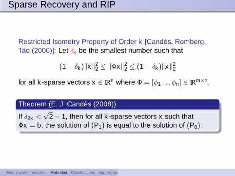
Restricted Isometry Property of Order k [Candès, Romberg,Tao (2006)]: Let δk be the smallest number such that
(1− δk )‖x‖22 ≤ ‖Φx‖2
2 ≤ (1 + δk )‖x‖22
for all k -sparse vectors x ∈ IRn where Φ = [φ1 . . . φn] ∈ IRm×n.
Theorem (E. J. Candès (2008))
If δ2k <√
2− 1, then for all k-sparse vectors x such thatΦx = b, the solution of (P1) is equal to the solution of (P0).
History and Introduction Main idea Constructions Approximation theory

Approximate Recovery and RIP
Basis Pursuit De-Noising (BPDN):
(Pε1) min‖x‖1 : ‖Φx − b‖2 ≤ ε
[Chen, Donoho, and Saunders (1999)]
Theorem (E. J. Candès (2008))
Suppose that the matrix Φ is given and b = Φx + e where‖e‖2 ≤ ε. If δ2k <
√2− 1, then
‖x? − x‖2 ≤ C0k−1/2σk (x)1 + C1ε,
where x? is the solution of (Pε1) and
σk (x)1 = minz∈Σk
‖x − z‖1.
Other Heuristics: Orthogonal Matching Pursuit, Mangasarian’sapproach, Bilinear formulation, etc.
History and Introduction Main idea Constructions Approximation theory

End of Part I.
History and Introduction Main idea Constructions Approximation theory

Construction of CS Matrices
Good compressive sensing (CS) matrices:
Known Result for Random matrices
Known reconstruction bounds for matrices with entriesdrawn at random from various probability distributions:
k ≤ Cm/ log(n/m).
Specific recipes include Gaussian, Bernoulli and otherclassical matrix ensembles.
Particular case: there is a probabilistic construction ofmatrices Φ of size m× n with entries ± 1√
m satisfying RIP
of order k with the above bound.
History and Introduction Main idea Constructions Approximation theory

Probabilistic Construction of CS Matrices
Introduce the Concentration of Measure Inequality (CMI)property on a probability space (Ω, %)
Suppose Φ = Φ(ω) is a collection of random m × nmatrices
Property PO(δ): the collection is said to have CMI if, foreach x ∈ IRn, there is a set Ω0(x , δ) ⊂ Ω s.t.
(1− δ)‖x‖2 ≤ ‖Φx‖2 ≤ (1 + δ)‖x‖2, ω ∈ Ω(x , δ)
and %(Ω(x , δ)c) ≤ C0e−c0mδ2
Gaussian, Bernoulli and many other families have thisproperty
History and Introduction Main idea Constructions Approximation theory
Property PO and the JL Lemma
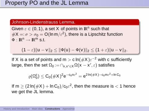
Johnson-Lindenstrauss Lemma.
Given ε ∈ (0, 1), a set X of points in IRn such that#X =:σ > σ0 = O(ln m/ε2), there is a Lipschitz functionΦ : IRn → IRm s.t.
(1− ε)‖u − v‖2 ≤ ‖Φ(u)− Φ(v)‖2 ≤ (1 + ε)‖u − v‖2.
If X is a set of points and m > c ln(#X )ε−2 with c sufficientlylarge, then the set Ω0 :=∩x ,x ′∈X Ω(x − x ′, ε) satisfies
%(Ωc0) ≤ C0(#X )2e−c0nε2
= e2 ln(#X)−c0mε2+ln C0
If m ≥ (2 ln(#X ) + ln C0)/c0ε2, then the measure is < 1 hence
we get the JL lemma.
History and Introduction Main idea Constructions Approximation theory

The JL Lemma and RIP
If k ≤ cm/ ln(n/m) and Φ satisfies JL, then we have RIP oforder k
For c sufficiently small, the probability that a Gaussianemsemble satisfies RIP is 1− Ce−cm
If we have a collection of O(ecm) bases, then a randomdraw of Gaussian will satisfy RIP with respect to all ofthese bases simultaneously
Basic reason why this works
Pr[∣∣∣‖Φ(ω)x‖2
`2− ‖x‖2
`2
∣∣∣ ≥ ε‖x‖2`2
]≤ 2e−mc0(ε), 0 < ε < 1.
History and Introduction Main idea Constructions Approximation theory

Deterministic Construction of CS Matrices
Difficulties in Deterministic Case
[DeVore]: Proposes a deterministic constructions of order
k ≤ C√
m log n/ log(n/m)
which is still far from probabilistic results.
Very recent ideas
Find deterministic constructions with better bounds
using bipartite expander graphs [Indyk, Hassibi, Xu];
using structured matrices such as Toeplitz, cyclic,generalized Vandermonde matrices.
Subgoal: deterministic polynomial time algorithm forconstructing good CS matrices.
Holy grail: k ≤ Cm/ log(n/m) – achievable for randommatrices but not yet in deterministic constructions.
History and Introduction Main idea Constructions Approximation theory

Connections with approximation theory
Cohen, Dahmen, DeVore [2009]: Compressed sensing andbest k -term approximation, JAMS.
Best k -term approximation error:
σk (x)X := infz∈Σk
‖x − z‖X .
Encoder-decoder viewpoint
The matrix Φ serves as an encoder producing y = Φx . Toextract x / approximation to x , use a decoder ∆ (notnecessarily linear). Thus
∆(y) = ∆(Φx) approximates x .
History and Introduction Main idea Constructions Approximation theory

Performance of encoders-decoders
Performance of encoder-decoder pairs
Ask for the largest value of k s.t.
x ∈ Σk =⇒ ∆(Φx) = x .
Ask for the largest value of k s.t., for a given class K ,
En(K )X ≤ Cσk (K )X , where
En(K )X := inf(Φ,∆)
supx∈K
‖x −∆(Φx)‖,
σk (K )X := supx∈K
σk (X ).
A pair (Φ,∆) is called instance-optimal of order k with constantC for the space X is
‖x −∆(Φx)‖X ≤ Cσk (x)X
for all x ∈ X with a constant C independent of k and n.History and Introduction Main idea Constructions Approximation theory

Connection with Gelfand widths
Gelfand widths
For K a compact set in X and m ∈ IN, the Gelfand width of K oforder m is
dm(K )X := infcodimY≤m
sup‖x‖X : x ∈ K ∩ Y.
Basic result
Lemma. Let K ⊂ IRn be symmetric, i.e., K = −K , and satisfyK + K ⊂ C0K for some C0. If X ⊆ IRn is any normed space,then
dm(K )X ≤ Em(K )X ≤ C0dm(K )X , 1 ≤ m ≤ n.
History and Introduction Main idea Constructions Approximation theory
Orders of Gelfand widths
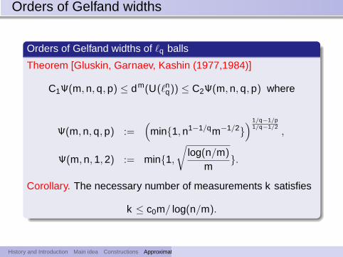
Orders of Gelfand widths of `q balls
Theorem [Gluskin, Garnaev, Kashin (1977,1984)]
C1Ψ(m, n, q, p) ≤ dm(U(`nq)) ≤ C2Ψ(m, n, q, p) where
Ψ(m, n, q, p) :=(
min1, n1−1/qm−1/2) 1/q−1/p
1/q−1/2,
Ψ(m, n, 1, 2) := min1,
√log(n/m)
m.
Corollary. The necessary number of measurements k satisfies
k ≤ c0m/ log(n/m).
History and Introduction Main idea Constructions Approximation theory

Instance optimality and the null space of Φ
Denote N :=N (Φ) :=x : Φx = 0.
Uniqueness of recovery
Lemma. For an m × n matrix Φ and for 2k ≤ m, the followingare equivalent:
There is a decoder ∆ s.t. ∆(Φx) = x for all x ∈ Σk .
Σ2k ∩N = 0.For any set T with #T = 2k , the matrix ΦT has rank 2k .
For any T as above, the matrix Φ∗T ΦT is positive definite.
History and Introduction Main idea Constructions Approximation theory

Approximate recovery
Approximation to accuracy σk
Theorem [Cohen, Dahmen, DeVore (2009)]. Given an m × nmatrix Φ, a norm ‖ · ‖X and a value of k , a sufficient conditionthat there exists a decoder ∆ s.t.
‖x −∆(Φx)‖X ≤ Cσk (x)X
is that‖η‖X ≤ C/2 · σ2k (η)X , η ∈ N .
A necessary condition is that
‖η‖X ≤ C · σ2k (η)X , η ∈ N .
This gives rise to the null space property (in X of order 2k ):
‖η‖X ≤ C · σ2k (η)X , η ∈ N .
History and Introduction Main idea Constructions Approximation theory
The null space property
Approximation and the null space property
Corollary [Cohen, Dahmen, DeVore (2009)].Suppose that X is an lnp space, k ∈ IN and Φ is an encodingmatrix. If Φ has the null space property in X of order 2k withconstant C/2, then there exists a decoder ∆ so that
‖x −∆(Φx)‖X ≤ Cσk (x)X .
Conversely, the validity of the above condition for some decoder∆ implies that Φ has the null space property in X of order 2kwith constant C.
History and Introduction Main idea Constructions Approximation theory

One of the main results, revisited
RIP and good encoder-decoder pairs
Theorem [Candès-Romberg-Tao (2006)]. Let Φ be any matrixwith satisfies the RIP of order 3k with δ3k ≤ δ < (
√2− 1)2/3.
Define the decoder ∆ by
∆(y) := argminΦz=y ‖z‖`1 .
Then (Φ,∆) satisfies
‖x −∆(Φx)‖X ≤ Cσk (x)X
in X = `1 with C = 2√
2+2−(2√
2−2)δ√2−1−(
√2+1)δ
.
History and Introduction Main idea Constructions Approximation theory

The End.
History and Introduction Main idea Constructions Approximation theory