“Old View” of Perception vs. “New View” -...

Autonomous Mobile Robots, Chapter 4

© R. Siegwart, I. Nourbakhsh (Adapted by Parker)

“Old View” of Perception vs. “New View”

Traditional (“old view”) approach: Perception considered in isolation (i.e., disembodied)

Perception “as king” (e.g., computer vision is “the” problem)

Universal reconstruction (i.e., 3D world models)



“New View” of Perception

Perception without the context of action is meaningless.

Action-oriented perception Perceptual processing tuned to meet motor activities’ needs

Expectation-based perception Knowledge of world can constrain interpretation of what is present in

world

Focus-of-attention methods Knowledge can constrain where things may appear in the world

Active perception Agent can use motor control to enhance perceptual processing via sensor

positioning

Perceptual classes: Partition world into various categories of potential interaction



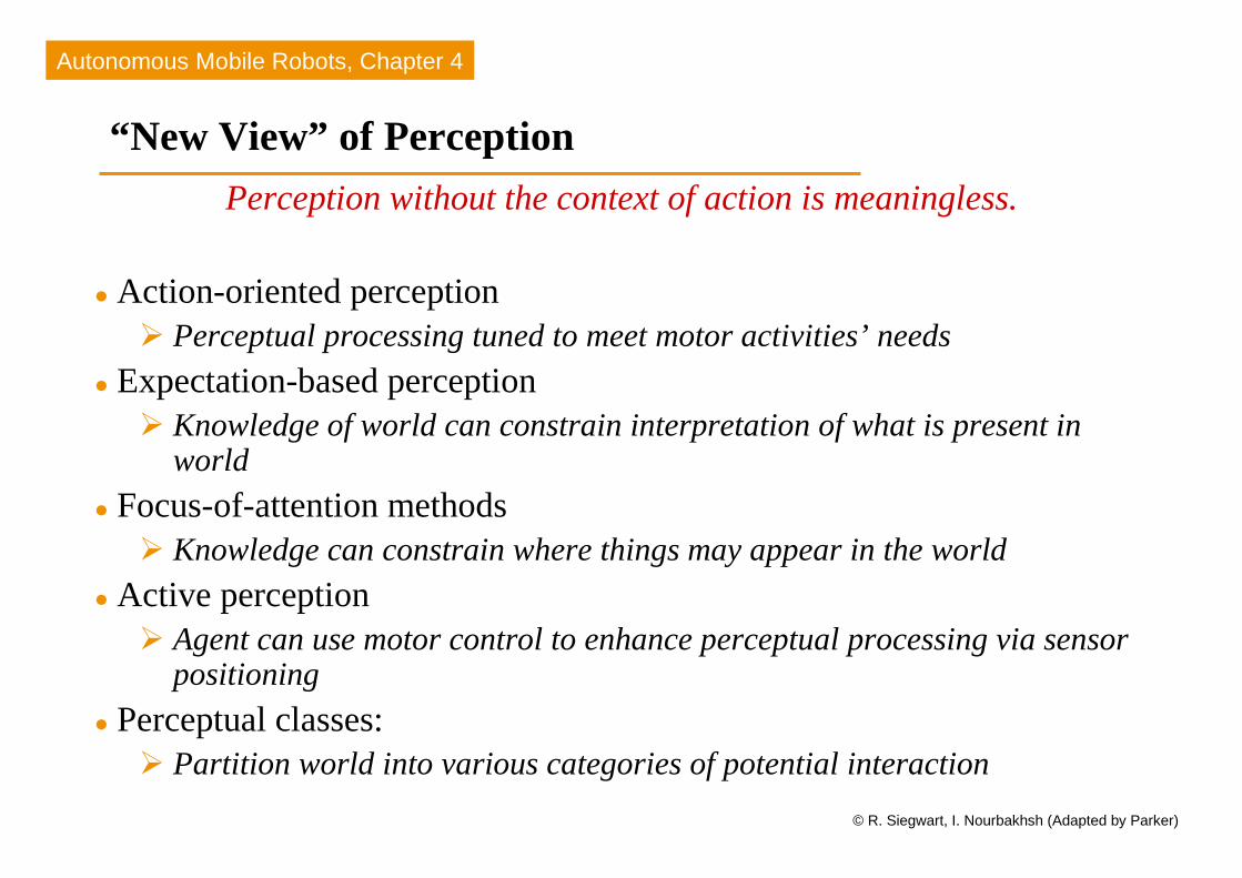
Consequence of “New View”

Purpose of perception is motor control, not representations

Multiple parallel processesthat fit robot’s different behavioral needs are used

Highly specialized perceptual algorithmsextract necessary information and no more.

Perception is conducted on a “need-to-know” basis



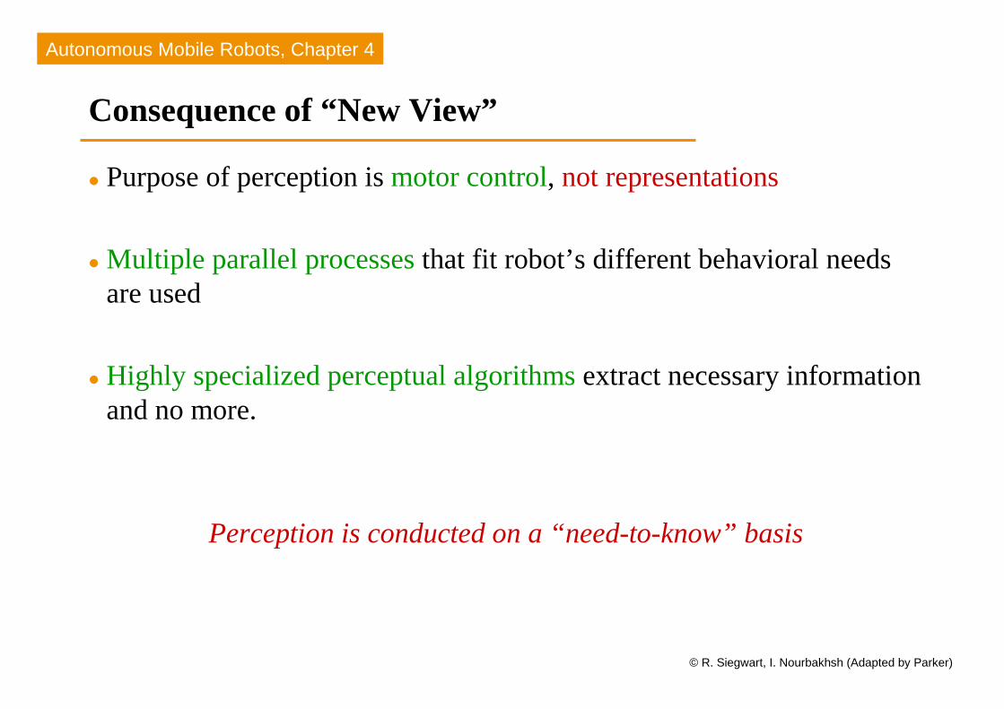
Complexity Analysis of New Approach is Convincing

Bottom-up “general visual search task” where matching is entirely data driven: Shown to be NP-complete (i.e., computationally intractable)

Task-directed visual search: Has linear-time complexity (Tsotsos 1989) Tractability results from optimizing the available resources dedicated to

perceptual processing (e.g., using attentional mechanisms)

Significance of results for autonomous robotics cannot be understated: “Any behaviorist approach to vision or robotics must deal with the inherent

computational complexity of the perception problem: otherwise the claim that those approaches scale up to human-line behavior is easily refuted.” (Tsotsos 1992, p. 140)

[Tsotsos, 1989] J. Tsotsos, “The Complexity of Perceptual Search Tasks”, Proc. of Int’l. Joint Conf. On Artificial Intelligence ’89, Detroit, MI, pp. 1571-77.

[Tsotsos, 1992] J. Tsotsos, “On the Relative Complexity of Active versus Passive Visual Search”, International Journal of Computer Vision, 7 (2): 127-141.



Primary Purpose of Perceptual Algorithms…

… is to support particular behavioral needs

Directly analogous with general results we’ve discussed earlier regarding “hierarchical” robotic control vs. “behavior-based/reactive” robotic control



Review: Laser Line Extraction (1)

Least Squares

Weighted Least Squares

4.3.1

ρρρρρρρρii

θθθθθθθθii



Features Based on Range Data: Line Extraction (2)

17 measurements

error (σ) proportional to ρ2

weighted least squares:

4.3.1



Segmentation for Line Extraction

4.3.1



Proximity Sensors

Measure relative distance (range) between sensor and objects in environment

Most proximity sensors are active

Common Types: Sonar (ultrasonics)

Infrared (IR)

Bump and feeler sensors



Sonar (Ultrasonics)

Refers to any system that achieves ranging through sound

Can operate at different frequencies

Very common on indoor and research robots

Operation: Emit a sound

Measure time it takes for

sound to return

Compute range based

on time of flightSonar



Reasons Sonar is So Common

Can typically give 360o coverage as polar plot

Cheap (a few $US)

Fast (sub-second measurement time)

Good range – about 25 feet with 1” resolution over FOV of 30o



Ultrasonic Sensor (time of flight, sound)

transmit a packet of (ultrasonic) pressure waves

distance d of the echoing object can be calculated based on the propagation speed of sound c and the time of flight t.

The speed of sound c (340 m/s) in air is given by

where

: ration of specific heats

R: gas constant

T: temperature in degree Kelvin

TRc ..γ=

2

.tcd =

γ

4.1.6



Ultrasonic Sensor (time of flight, sound)

typically a frequency: 40 - 180 kHz generation of sound wave: piezo transducer

transmitter and receiver separated or not separated

sound beam propagates in a cone like manner opening angles around 20 to 40 degrees regions of constant depth segments of an arc (sphere for 3D)

Typical intensity distribution of a ultrasonic sensor

-30°

-60°

0°

30°

60°

Amplitude [dB]

measurement cone

4.1.6



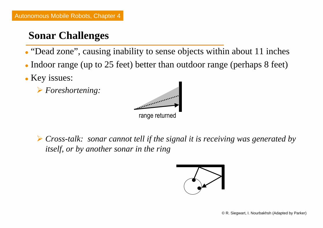
Sonar Challenges “Dead zone”, causing inability to sense objects within about 11 inches

Indoor range (up to 25 feet) better than outdoor range (perhaps 8 feet)

Key issues: Foreshortening:

Cross-talk: sonar cannot tell if the signal it is receiving was generated by itself, or by another sonar in the ring

range returned



Sonar Challenges (con’t.)

Key issues (con’t.)Specular reflection: when wave form hits a surface at an acute and bounces

away

Specular reflection also results in signal reflecting differently from different materialsE.g., cloth, sheetrock, glass, metal, etc.

Common method of dealing with spurious readings:Average three readings (current plus last two) from each sensor



Infrared (IR) Active proximity sensor

Emit near-infrared energy and measure amount of IR light returned

Range: inches to several feet, depending on light frequency andreceiver sensitivity

Typical IR: constructed from LEDs, which have a range of 3-5 inches

Issues: Light can be “washed out” by bright ambient lighting

Light can be absorbed by dark materials



Bump and Feeler (Tactile) Sensors

Tactile (touch) sensors: wired so that when robot touches object, electrical signal is generated using a binary switch

Sensitivity can be tuned (“light” vs. “heavy” touch), although it is tricky

Placement is important (height, angular placement)

Whiskers on Genghis

Bump sensors



Proprioceptive Sensors

Sensors that give information on the internal state of the robot, such as: Motion

Position (x, y, z)

Orientation (about x, y, z axes)

Velocity, acceleration

Temperature

Battery level

Example proprioceptive sensors: Encoders (dead reckoning) Inertial navigation system (INS) Global positioning system (GPS) Compass Gyroscopes



Dead Reckoning/Odometry/Encoders

Purpose: To measure turning distance of motors (in terms of numbers of

rotations), which can be converted to robot translation/rotation distance

If gearing and wheel size known, number of motor turns number of wheel turns estimation of distance robot has traveled

Basic idea in hardware implementation:

Device to count number of “spokes” passing by



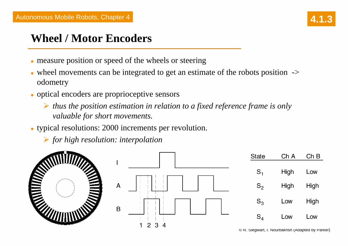
Wheel / Motor Encoders

measure position or speed of the wheels or steering

wheel movements can be integrated to get an estimate of the robots position -> odometry

optical encoders are proprioceptive sensors

thus the position estimation in relation to a fixed reference frame is only valuable for short movements.

typical resolutions: 2000 increments per revolution.

for high resolution: interpolation

4.1.3



Encoders (con’t.) Challenges/issues:

Motion of wheels not corresponding to robot motion, e.g., due to wheel spinning

Wheels don’t move but robot does, e.g., due to robot sliding

Error accumulates quickly, especially due to turning:

Red line indicates estimated robot position due to

encoders/odometry/dead reckoning.

Begins accurately, but errors accumulate quickly

Robot start positio

n



Another Example of Extent of Dead Reckoning Errors

Plot of overlaid laser scans overlaid based strictly on odometry:



Inertial Navigation Sensors (INS)

Inertial navigation sensors: measure movements electronically through miniature accelerometers

Accuracy: quite good (e.g., 0.1% of distance traveled) if movements are smooth and sampling rate is high

Problem for mobile robots: Expensive: $50,000 - $100,000 USD

Robots often violate smooth motion constraint

INS units typically large



Heading Sensors

Heading sensors can be proprioceptive (gyroscope, inclinometer) or exteroceptive (compass).

Used to determine the robots orientation and inclination.

Allow, together with an appropriate velocity information, to integrate the movement to an position estimate. This procedure is called dead reckoning (ship navigation)

4.1.4



Compass

Since over 2000 B.C.

when Chinese suspended a piece of naturally magnetite from a silk thread and used it to guide a chariot over land.

Magnetic field on earth

absolute measure for orientation.

Large variety of solutions to measure the earth magnetic field

mechanical magnetic compass

direct measure of the magnetic field (Hall-effect, magnetoresistive sensors)

Major drawback

weakness of the earth field

easily disturbed by magnetic objects or other sources

not feasible for indoor environments

4.1.4



Gyroscope

Heading sensors, that keep the orientation to a fixed frame absolute measure for the heading of a mobile system.

Two categories, the mechanical and the optical gyroscopes Mechanical Gyroscopes

Standard gyro

Rated gyro

Optical Gyroscopes Rated gyro

4.1.4



Mechanical Gyroscopes

Concept: inertial properties of a fast spinning rotor gyroscopic precession

Angular momentum associated with a spinning wheel keeps the axis of the gyroscope inertially stable.

Reactive torque t (tracking stability) is proportional to the spinning speed w, the precession speed W and the wheels inertia I.

No torque can be transmitted from the outer pivot to the wheel axis spinning axis will therefore be space-stable

Quality: 0.1° in 6 hours

If the spinning axis is aligned with the north-south meridian, the earth’s rotation has no effect on the gyro’s horizontal axis

If it points east-west, the horizontal axis reads the earth rotation

Ω= ωτ I

4.1.4



Rate gyros

Same basic arrangement shown as regular mechanical gyros

But: gimble(s) are restrained by a torsional spring enables to measure angular speeds instead of the orientation.

Others, more simple gyroscopes, use Coriolis forces to measure changes in heading.

4.1.4



Optical Gyroscopes

First commercial use started only in the early 1980 when they where first installed in airplanes.

Optical gyroscopes angular speed (heading) sensors using two monochromic light (or laser)

beams from the same source.

On is traveling in a fiber clockwise, the other counterclockwise around a cylinder

Laser beam traveling in direction of rotation slightly shorter path -> shows a higher frequency

difference in frequency ∆f of the two beams is proportional to the angular velocity Ω of the cylinder

New solid-state optical gyroscopes based on the same principle are build using microfabrication technology.

4.1.4



Ground-Based Active and Passive Beacons

Elegant way to solve the localization problem in mobile robotics

Beacons are signaling guiding devices with a precisely known position

Beacon base navigation is used since the humans started to travel

Natural beacons (landmarks) like stars, mountains or the sun

Artificial beacons like lighthouses

The recently introduced Global Positioning System (GPS) revolutionized modern navigation technology

Already one of the key sensors for outdoor mobile robotics

For indoor robots GPS is not applicable,

Major drawback with the use of beacons in indoor:

Beacons require changes in the environment -> costly.

Limit flexibility and adaptability to changing environments.

4.1.5



Global Positioning System (GPS) (1)

Developed for military use

Recently it became accessible for commercial applications

24 satellites (including three spares) orbiting the earth every 12 hours at a height of 20.190 km.

Four satellites are located in each of six planes inclined 55 degrees with respect to the plane of the earth’s equators

Location of any GPS receiver is determined through a time of flight measurement

Technical challenges:

Time synchronization between the individual satellites and the GPS receiver

Real time update of the exact location of the satellites

Precise measurement of the time of flight

Interferences with other signals

4.1.5




4.1.5




Time synchronization: atomic clocks on each satellite monitoring them from different ground stations.

Ultra-precision time synchronization is extremely important electromagnetic radiation propagates at light speed,

Roughly 0.3 m per nanosecond. position accuracy proportional to precision of time measurement.

Real time update of the exact location of the satellites: monitoring the satellites from a number of widely distributed ground stations master station analyses all the measurements and transmits the actual position to each of

the satellites Exact measurement of the time of flight

the receiver correlates a pseudocode with the same code coming from the satellite The delay time for best correlation represents the time of flight. quartz clock on the GPS receivers are not very precise the range measurement with four satellite allows to identify the three values (x, y, z) for the position and the clock correction ∆T

Recent commercial GPS receiver devices allows position accuracies down to a couple meters.

4.1.5



Differential Global Positioning System (DGPS)

Satellite-based sensing system

Robot GPS receiver:

Triangulates relative to signals from 4 satellites

Outputs position in terms of latitude, longitude, altitude, and change in time

Differential GPS:

Improves localization by using two GPS receivers

One receiver remains stationary, other is on robot

Sensor Resolution:

GPS alone: 2-3 meters

DGPS: up to a few centimeters



Example DGPS Sensors on Robots



DGPS Challenges

Does not work indoors in most buildings

Does not work outdoors in “urban canyons” (amidst tall buildings)

Forested areas (i.e., trees) can block satellite signals

Cost is high (several thousand $$)



Computer Vision Computer vision:processing data from any modality that uses the

electromagnetic spectrum which produces an image Image:

A way of representing data in a picture-like format where there is a direct physical correspondence to the scene being imaged

Results in a 2D array or grid of readings Every element in array maps onto a small region of space Elements in image array are called pixels

Modality determines what image measures: Visible light measures value of light (e.g. color or gray

level) Thermal measures heat in the given region

Image function:converts signal into a pixel value

CMU Cam

(for color blob tracking)

Pan-Tilt-Zoom camera

Stereo vision

Omnidirectional

Camera



Types of Computer Vision

Computer vision includes: Cameras (produce images over same

electromagnetic spectrum that humans see)

Thermal sensors

X-rays

Laser range finders

Synthetic aperature radar (SAR)

Thermal image

SAR image (of U.S. capitol building)3D Laser scanner image



Computer Vision is a Field of Study on its Own

Computer vision field has developed algorithms for: Noise filtering

Compensating for illumination problems

Enhancing images

Finding lines

Matching lines to models

Extracting shapes and building 3D representations

However, autonomous mobile robots operating in dynamic environments must use computationally efficient algorithms; not all vision algorithms can operate in real-time



CCD (Charge Coupled Device) Cameras

CCD technology:Typically, computer vision on autonomous mobile robots is from a video camera, which uses CCD technology to detect visible light

Output of most cameras:analog; therefore, must be digitized for computer use

Framegrabber: Card that is used by the computer, which accepts an analog camera signal

and outputs the digitized results

Can produce gray-scale or color digital image

Have become fairly cheap – color framegrabbers cost about $200-$500.



Representation of Color

Color measurements expressed as three color planes – red,green, blue (abbreviated RGB)

RGB usually represented as axes of 3D cube, with values ranging from 0 to 255 for each axis

Black (0,0,0)

White (255,255,255)

Blue(0,0,255)

Green (0,255,0)

Red (255,0,0)Yellow (255,255,0)

Cyan (0,255,255)

Magenta(255,0,255)



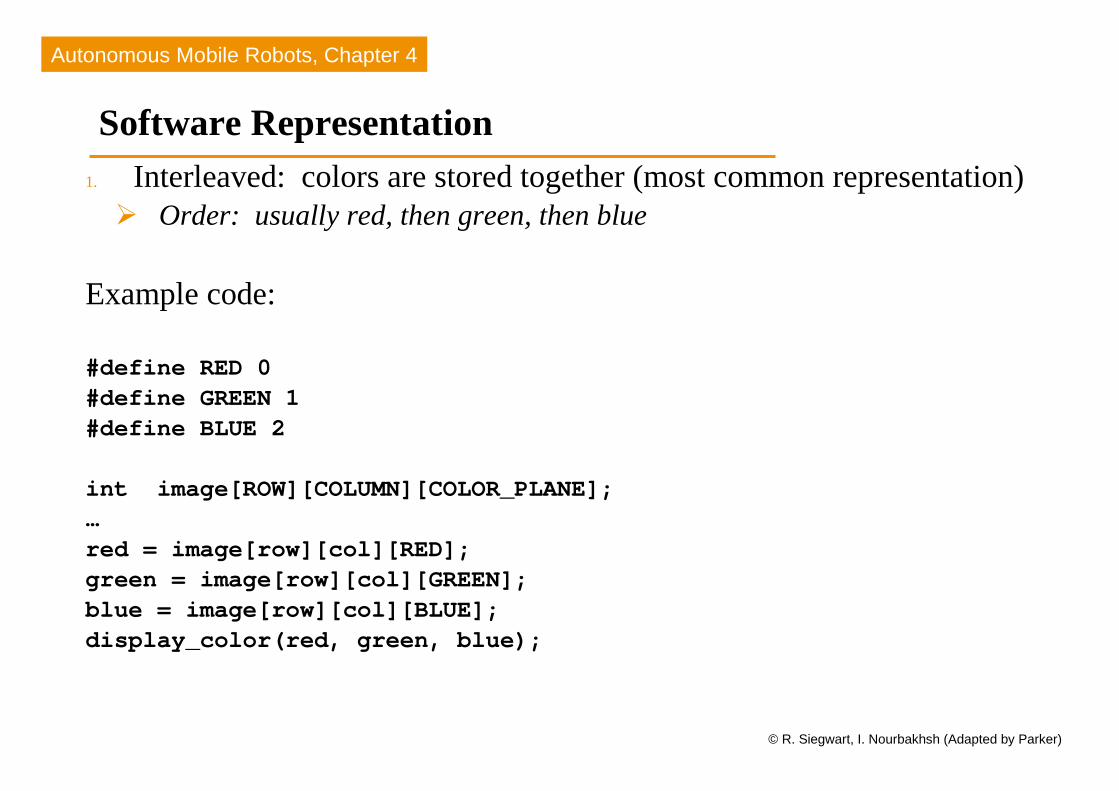
Software Representation1. Interleaved: colors are stored together (most common representation)

Order: usually red, then green, then blue

Example code:

#define RED 0#define GREEN 1#define BLUE 2

int image[ROW][COLUMN][COLOR_PLANE];…red = image[row][col][RED];green = image[row][col][GREEN];blue = image[row][col][BLUE];display_color(red, green, blue);



Software Representation (con’t.)

2. Separate: colors are stored as 3 separate 2D arrays

Example code:

int image_red[ROW][COLUMN];

int image_green[ROW][COLUMN];

int image_blue[ROW][COLUMN];

…

red = image_red[row][col];

green = image_green[row][col];

blue = image_blue[row][col];

display_color(red, green, blue);



Challenges Using RGB for Robotics

Color is function of: Wavelength of light source

Surface reflectance

Sensitivity of sensor

Color is not absolute; Object may appear to be at different color values at different distances to

due intensity of reflected light



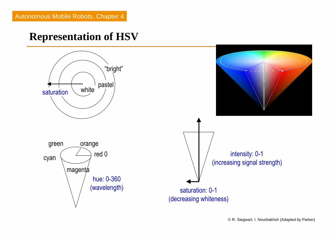
Better: Device which is sensitive to absolute wavelength

Better: Hue, saturation, intensity (or value) (HSV) representation of color

Hue: dominant wavelength, does not change with robot’s relative position or object’s shape

Saturation:lack of whiteness in the color (e.g., red is saturated, pink is less saturated)

Intensity/Value:quantity of light received by the sensor

Transforming RGB to HSV



Representation of HSV

hue: 0-360

(wavelength)

red 0

orangegreen

cyan

magenta

“bright”

pastelwhitesaturation

intensity: 0-1

(increasing signal strength)

saturation: 0-1

(decreasing whiteness)



HSV Challenges for Robotics

Requires special cameras and framegrabbers

Expensive equipment

Alternative: Use algorithm to convert -- Spherical Coordinate Transform (SCT) Transforms RGB data to a color space that more closely duplicates

response of human eye

Used in biomedical imaging, but not widely used for robotics

Much more insensitive to lighting changes



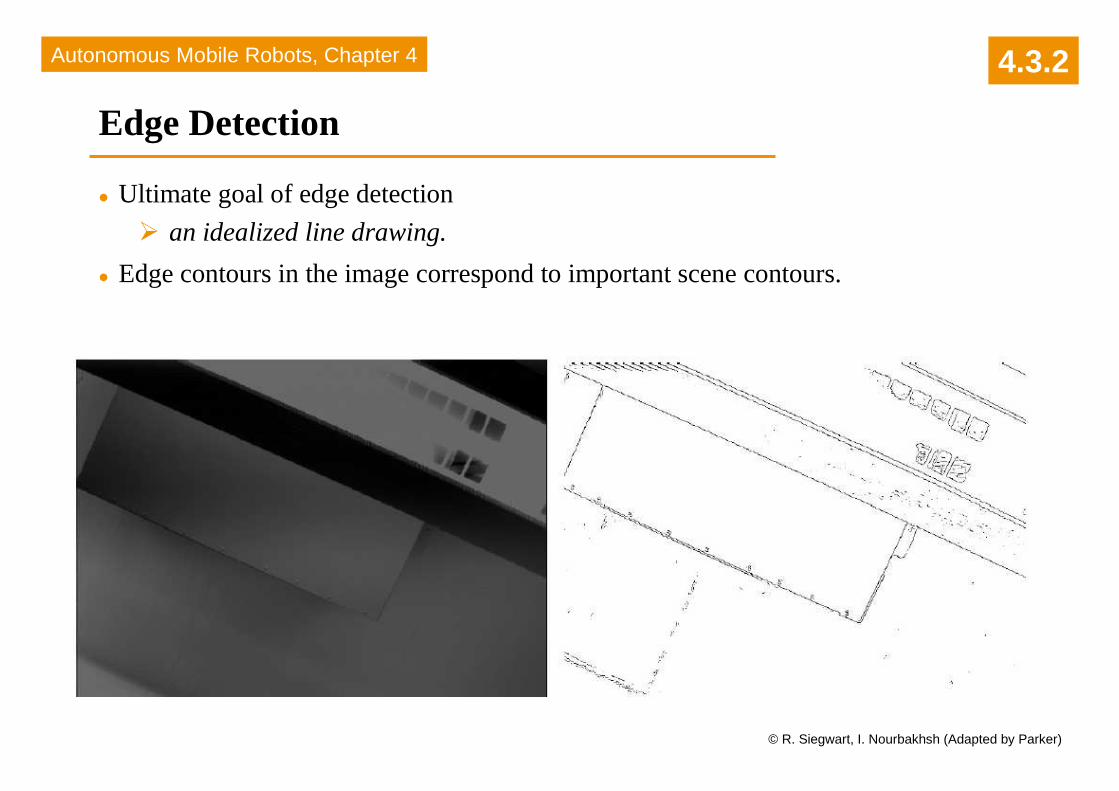
Edge Detection

Ultimate goal of edge detection

an idealized line drawing.

Edge contours in the image correspond to important scene contours.

4.3.2



Region Segmentation

Region Segmentation:most common use of computer vision in robotics, with goal to identify region in image with a particular color

Basic concept: identify all pixels in image which are part of the region, then navigate to the region’s centroid

Steps: Threshold all pixels which share same color (thresholding)

Group those together, throwing out any that don’t seem to be in same area as majority of the pixels (region growing)



Example Code for Region Segmentation

for (i=0; i<numberRows; i++)

for (j=0; j<numberColumns; j++)

if (((ImageIn[i][j][RED] >= redValueLow)

&& (ImageIn[i][j][RED] <= redValueHigh))

&& ((ImageIn[i][j][GREEN] >= greenValueLow)

&& (ImageIn[i][j][GREEN] <= greenValueHigh))

&& ((ImageIn[i][j][BLUE] >= blueValueLow)

&& (ImageIn[i][j][BLUE] <= blueValueHigh)))

ImageOUT[i][j] = 255;

else

ImageOut[i][j] = 0;

Note range of readings required due to non-absolute color values



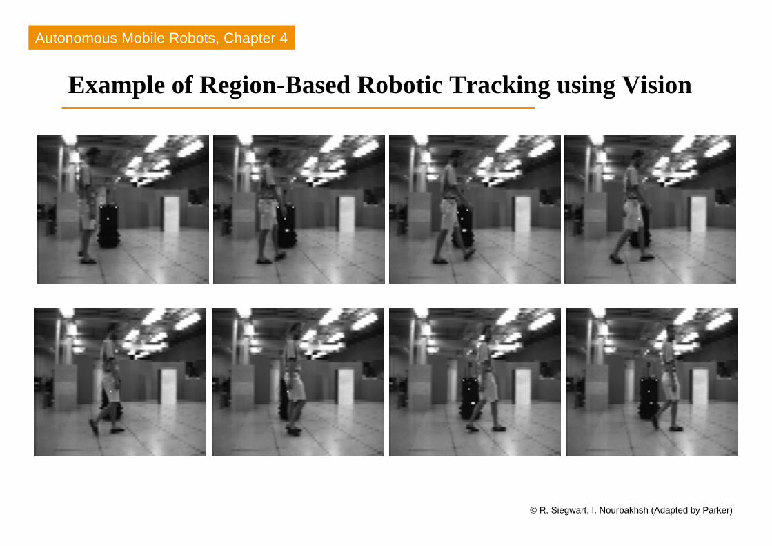
Example of Region-Based Robotic Tracking using Vision



Another Example of Vision-Based Robot Detection Using Region Segmentation



Color Histogramming Color histogramming:

Used to identify a region with several colors

Way of matching proportion of colors in a region

Histogram: Bar chart of data

User specifies range of values for each bar (called buckets)

Size of bar is number of data points whose value falls into the range for that bucket

Example:

0-31 64-95 128-159 192-223

32-63 96-127 160-191 224-251



Color Histograms (con’t.)

Advantage for behavior-based/reactive robots: Histogram IntersectionColor histograms can be subtracted from each other to determine if

current image matches a previously constructed histogram

Subtract histograms bucket by bucket; different indicates # of pixels that didn’t match

Number of mismatched pixels divided by number of pixels in image gives percentage match = Histogram Intersection

This is example of local, behavior-specific representation that can be directly extracted from environment



Range from Vision

Perception of depth from stereo image pairs, or from optic flow

Stereo camera pairs: range from stereo

Key challenge: how does a robot know it is looking at the same point in two images? This is the correspondence problem.



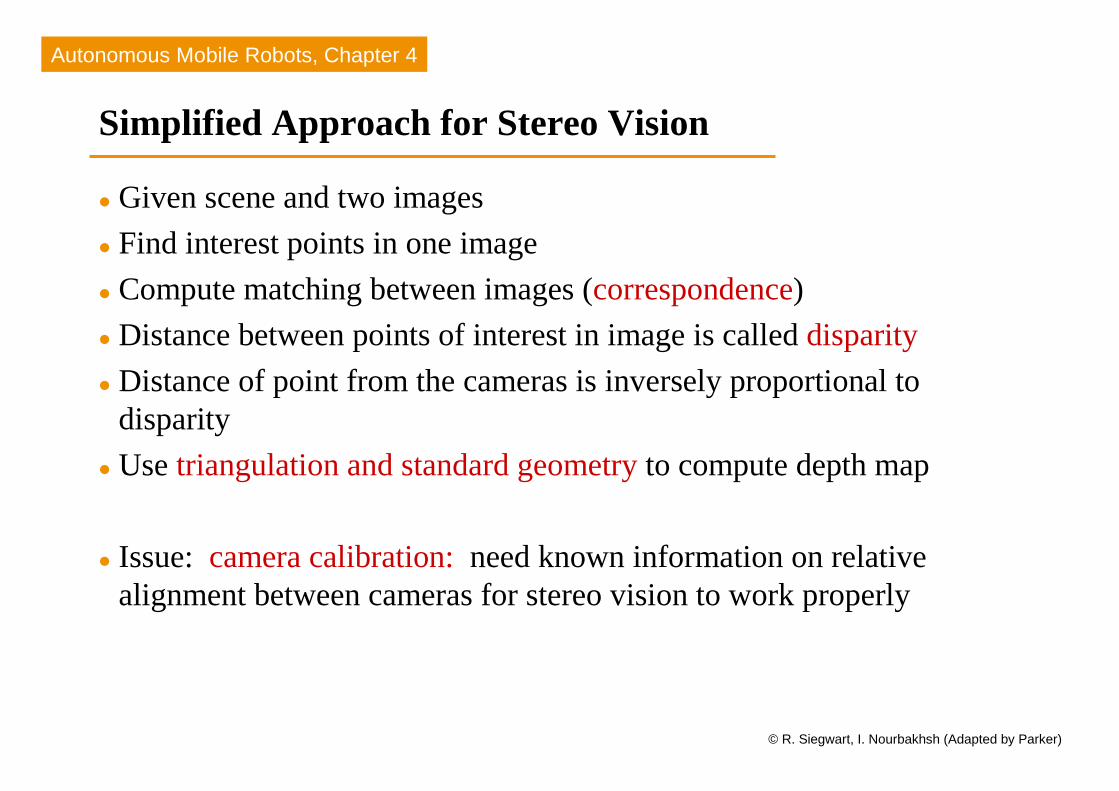
Simplified Approach for Stereo Vision

Given scene and two images

Find interest points in one image

Compute matching between images (correspondence)

Distance between points of interest in image is called disparity

Distance of point from the cameras is inversely proportional to disparity

Use triangulation and standard geometryto compute depth map

Issue: camera calibration:need known information on relative alignment between cameras for stereo vision to work properly

“Old View” of Perception vs. “New View” -...

Documents

Transcript of “Old View” of Perception vs. “New View” -...