Okkonen Masters Thesis - WARP Project

DEPARTMENT OF COMPUTER SCIENCE AND ENGINEERING

Juha Okkonen

UNIFORM LINEAR ADAPTIVE ANTENNAARRAY BEAMFORMING IMPLEMENTATION

WITH A WIRELESS OPEN-ACCESSRESEARCH PLATFORM

Master’s ThesisDegree Programme in Computer Science and Engineering

May 2013

Okkonen J. (2013) Uniform linear adaptive antenna array beamforming imple-mentation with a wireless open-access research platform. University of Oulu, De-partment of Computer Science and Engineering. Master’s Thesis, 58 p.

ABSTRACT

The wireless communication techniques are expected to keep up with the increas-ing demand for capacity. The increased number of users is the primary culpritwith the contribution of more data intensive applications. Multiple access divi-sions based on time, frequency and code have been widely explored and spaceremains the most promising option for future capacity improvements.

Beamforming is an advanced space division multiple access (SDMA) technique,where an array of antennas spatially filters signals based on their capture time ateach element. Unless the signal arrives orthogonally at the array, the capturetimes differ based on the direction of arrival (DOA).

Two non-adaptive beamforming techniques were implemented with a wirelessopen-access research platform (WARP). The first technique was the conventionalbeamforming, where the main beam is steered towards the DOA. The second tech-nique was the null-steering beamforming, where, in addition to steering the mainbeam, minimum gains (nulls) are placed towards interfering sources for suppres-sion.

The measured beamforms, for receive beamforming, yielded a good main beamperformance with respect to the theoretical beamforms, although the null-steeringhad some deviations. The null levels were about -20 dB and -28 dB for the conven-tional and null-steering beamforming, respectively. Sidelobe levels were slightlyhigher, at around -10 dB, and wider for the conventional beamforming. In thenull-steering, the sidelobe levels were somewhat or considerably higher and widerdepending on the placement of nulls.

Keywords: adaptive antenna, beamforming, phased array, SDMA, smart an-tenna, uniform linear array, wireless open-access research platform

Okkonen J. (2013) Tasavälisen lineaarisen adaptiivisen antenniryhmän keilan-muodostuksen toteutus langattomalla tutkimusalustalla. Oulun yliopisto, Tietotek-niikan osasto. Diplomityö, 58 s.

TIIVISTELMÄ

Langattomilta tietoliikennetekniikoilta oletetaan yhä suurempaa kapasiteettia.Lisääntyneet käyttäjämäärät ovat suurin tekijä, mutta osansa on myös sovel-luksien suuremmilla tiedonsiirtovaatimuksilla. Aika-, taajuus- ja koodijakokana-voinnit ovat laajasti tutkittuja ja tilajakokanavointi (SDMA, space division mul-tiple access) on lupaavin vaihtoehto kapasiteetin kasvattamiselle tulevaisuudessa.

Keilanmuodostus on kehittynyt tilajakokanavointitekniikka, jossa antenniryh-mä erottelee signaalit avaruudessa eri antennien vastaanottoaikojen perusteella.Ellei signaali saavu ortogonaalisesti antenniryhmälle, vastaanottoajat eroavat toi-sistaan riippuen signaalin tulosuunnasta (DOA, direction of arrival).

Kaksi ei-adaptiivista keilanmuodostustekniikkaa toteutettiin langattomalla tut-kimusalustalla (WARP, wireless open-access research platform). Ensimmäinentekniikka oli klassinen keilanmuodostus, jossa pääkeila suunnataan kohti sig-naalin tulosuuntaa. Toinen tekniikka oli nollanohjausmenetelmä, jossa, pääkeilansuuntaamisen lisäksi, minimivahvistukset (nollat) suunnataan kohti häiriölähtei-tä niiden vaimentamiseksi.

Vastaanotossa mitatut keilanmuodot saavuttivat hyvän suorituskyvyn verrat-taessa niitä teoreettisiin keilanmuotoihin. Nollanmuodostusmenetelmällä oli kui-tenkin pieniä poikkeavuuksia. Nollatasot olivat noin -20 dB klassisella keilan-muodostuksella ja -28 dB nollanohjausmenetelmällä. Sivukeilatasot olivat hiemankorkeammat, -10 dB tasolla, ja leveämmät klassisessa keilanmuodostuksessa. Nol-lanohjausmenetelmässä sivukeilatasot olivat hieman tai merkittävästi korkeam-mat ja leveämmät riippuen nollien sijoitteluista.

Avainsanat: adaptiivinen antenni, keilanmuodostus, langaton tutkimusalusta, ta-savälinen lineaarinen ryhmä, tilajakokanavointi, vaiheistettu antenniryhmä, äly-antenni

TABLE OF CONTENTS

ABSTRACT

TIIVISTELMÄ

TABLE OF CONTENTS

FOREWORD

LIST OF SYMBOLS AND ABBREVIATIONS

1. INTRODUCTION 10

2. BEAMFORMING 152.1. Coordinate system . . . . . . . . . . . . . . . . . . . . . . . . . . . 162.2. Operating principle . . . . . . . . . . . . . . . . . . . . . . . . . . . 17

2.2.1. Fundamentals . . . . . . . . . . . . . . . . . . . . . . . . . . 172.2.2. Radio channel propagation . . . . . . . . . . . . . . . . . . . 182.2.3. Signal model . . . . . . . . . . . . . . . . . . . . . . . . . . 182.2.4. Assumptions . . . . . . . . . . . . . . . . . . . . . . . . . . 21

2.3. Implementation issues . . . . . . . . . . . . . . . . . . . . . . . . . 222.3.1. Array geometry . . . . . . . . . . . . . . . . . . . . . . . . . 222.3.2. Pattern multiplication . . . . . . . . . . . . . . . . . . . . . . 22

2.4. Performance impacting factors . . . . . . . . . . . . . . . . . . . . . 222.4.1. Number of elements . . . . . . . . . . . . . . . . . . . . . . 232.4.2. Element spacing . . . . . . . . . . . . . . . . . . . . . . . . 252.4.3. Scan angle . . . . . . . . . . . . . . . . . . . . . . . . . . . 272.4.4. Amplitude illumination . . . . . . . . . . . . . . . . . . . . . 29

2.5. Techniques . . . . . . . . . . . . . . . . . . . . . . . . . . . . . . . 292.5.1. Conventional . . . . . . . . . . . . . . . . . . . . . . . . . . 312.5.2. Null-steering . . . . . . . . . . . . . . . . . . . . . . . . . . 32

3. WIRELESS OPEN-ACCESS RESEARCH PLATFORM 363.1. FPGA board . . . . . . . . . . . . . . . . . . . . . . . . . . . . . . . 363.2. FPGA . . . . . . . . . . . . . . . . . . . . . . . . . . . . . . . . . . 363.3. Radio board . . . . . . . . . . . . . . . . . . . . . . . . . . . . . . . 373.4. WARPLab . . . . . . . . . . . . . . . . . . . . . . . . . . . . . . . . 38

4. CALIBRATION 404.1. Phase-locked loop calibration . . . . . . . . . . . . . . . . . . . . . . 404.2. Array manifold measurement . . . . . . . . . . . . . . . . . . . . . . 44

5. MEASUREMENTS 475.1. Measurement setup . . . . . . . . . . . . . . . . . . . . . . . . . . . 475.2. Receive beamforming . . . . . . . . . . . . . . . . . . . . . . . . . . 485.3. Transmit beamforming . . . . . . . . . . . . . . . . . . . . . . . . . 50

6. DISCUSSION 53

7. SUMMARY 55

8. REFERENCES 56

FOREWORD

The research work for this master’s thesis was carried out at the Centre for WirelessCommunications (CWC), Department of Communications Engineering (DCE), Uni-versity of Oulu. The thesis is part of a Reconfigurable Antenna Based Enhancement ofDynamic Spectrum Access Algorithms (RADSA) research project that was conductedin co-operation with the CWC and the Drexel University in Philadelphia, Pennsylva-nia, USA. The purpose of this thesis was to develop a reconfigurable direction selectiveantenna system, capable of directed transmission and reception, through adaptive an-tenna beamforming that was demonstrated with the Wireless Open-Access ResearchPlatform (WARP) environment.

I would like to express thanks to my supervisors M.Sc. Hannu Tuomivaara for hisguidance and advice and Dr. Harri Saarnisaari for his insight and feedback. I am verygrateful to Lic.Sc. Pekka Lilja, M.Sc. Marko Sonkki and Lic.Sc. Risto Vuohtoniemifor their assistance.

I would like to thank my fellow team members for a comfortable working atmo-sphere, especially M.Sc. Markku Jokinen for his help with the equipment. My thanksgo to the second examiner Dr. Timo Ojala for his comments and Dr. Pekka Pirinen forgiving the opportunity to work at the CWC.

I also thank M.Sc. Jari Sillanpää for technical support, M.Sc. Tuomo Hänninen forsupervision and the whole staff at the DCE including administrative personnel.

The research funding provided by the Finnish Funding Agency for Technology andInnovation (TEKES) is gratefully acknowledged.

Special thanks to my family and friends for their support.

Oulu, May 22th, 2013

Juha Okkonen

LIST OF SYMBOLS AND ABBREVIATIONS

[·]+ matrix pseudo inverse[·]∗ complex conjugate[·]−1 matrix inversion[·]H complex conjugate transpose[·]T transposeπ mathematical constant, ratio of a circle’s circumference to its diameter∈ set membership operatore[·] exponential function∑

summation operator| · | absolute valueE{·} expectation operatorlog10 common logarithmmax[·] maximum value

a(θ) steering vector as a function of incident anglea(ω) steering vector as a function of angular frequencyA steering matrixc speed of lightd element spacingf frequencyI identity matrixk wave numberM number of signal sourcesnm(t) noise at mth elementN number of elements in an arraypi ith signal source power measured at one the elements of the arrayps signal source powerP (θ) beamformer response as a function of incident angleP (ω) beamformer response as a function of angular frequencyP(w) beamformer mean output powerPN beamformer output noise powerr radial distance from originR correlation matrixRN noise correlation matrixsi(t) ith signalSNRin beamformer input signal-to-noise ratioSNRout beamformer output signal-to-noise ratioS source correlation matrixt timew∗m complex weight for mth antenna elementw weight vectorwC weight vector for conventional beamformerwNS weight vector for null-steeringx first coordinate in Cartesian system

xm(t) output of m antenna elementxms(t) signal induced on the mth element due to signal source sX number of phase offset measurementx(t) all the signals induced on all the elementsxs(t) signal induced on all the elements in the array due to signal source sy second coordinate in Cartesian systemy(t) beamformer outputz third coordinate in Cartesian system

αi PLL phase offset of radio board iδ PLL phase offset change due to propagation of signal in channelθ zenith angleθi angle of incidenceθrfl angle of reflectionθrfr angle of refractionλ wavelengthσ2n noise varianceτm propagation delay to mth antenna with respect to firstφ azimuth angleω angular frequency

AAS active antenna systemADC analog-to-digital converterAF array factorAGC automatic gain controlCF CompactFlashCWC Centre for Wireless CommunicationsDAC digital-to-analog converterdB decibelDBF digital beamforming/beamformerDCE Department of Communications EngineeringDIP dual in-line packageDOA direction of arrivalEM electromagneticFPGA field-programmable gate arrayGbps gigabits per secondGHz gigaHertzI in-phaseI/O input/outputI/Q in-phase/quadratureIF intermediate frequencyISM industrial, scientific and medicalJTAG Joint Test Action Groupkb kilobitLED light-emitting diodeLOS line-of-sightM2M machine-to-machine

MAC medium access controlMATLAB matrix laboratoryMb megabitMbps megabits per secondMGT multi-gigabit transceiverMHz megaHertzMIMO multiple input multiple outputMMSE minimum mean square errorMRA minimum redundancy arrayNLOS non-line-of-sightNNBW null-to-null beamwidthNRA null redundancy arrayNSN Nokia Siemens NetworksOTA over-the-airPC personal computerPHY physical layerPLL phase-locked loopQ quadrature-phaseRADSA Reconfigurable Antenna Based Enhancement of Dynamic Spectrum Access AlgorithmsRAM random access memoryRF radio frequencyRP radiation patternRS-232 recommended standard 232RSSI received signal strength indicatorRx receiver / reception / receiveSDMA space-division multiple accessSIR signal-to-interference ratioSNR signal-to-noise ratioSPI Serial Peripheral InterfaceSRAM static random access memoryTEKES Finnish Funding Agency for Technology and InnovationTx transmitter / transmission / transmitUART Universal Asynchronous Receiver TransmitterUCA uniform circular arrayULA uniform linear arrayUSB Universal Serial BusV voltWARP Wireless Open-Access Research PlatformZBT zero-bus-turnaround

10

1. INTRODUCTION

The wireless communications is facing an enormous challenge to satisfy the ever-increasing demand for capacity. The demand is primarily caused by an increasingnumber of users but also because of more data intensive applications. It is expectedthat the number of mobile Internet-connected devices is over 10 billion in 2016, ex-ceeding the number of people on Earth, estimated to be 7.3 billion. 8 billion of theseare personal mobile-ready devices and the remaining 2 billion are machine-to-machine(M2M) connections. The devices will be more powerful and hence are able to consumeand generate more data traffic. From 2011 to 2016, the mobile data traffic will increase18-fold, streamed content 28-fold and tablet traffic 62-fold. Smartphones, laptops andother portable devices will be responsible for about 90 % of all mobile data traffic by2016. Remaining 10 % belongs to M2M communication and residential broadbandmobile gateways, 5 % each. Mobile video alone, is 71 % of all mobile data traffic.Mobile data traffic is expected to outgrow fixed data traffic by three times by the endof 2016. [1]

Interference is one of the major problems in radio communications. The interferencecan be caused by the signal itself or by other users [2]. Signal can interfere with itselfdue to multipath components, where the signal is combined with another version ofthe signal that is delayed because of another propagation path. Interference from otherusers can be either unintentional or intentional [2]. Unintentional interference is causedby nonidealities in the transmitter or using the same or adjacent channel. Intentionalinterference or jamming is radiation directed towards a target for the purpose of tryingto prevent it from receiving the desired signal.

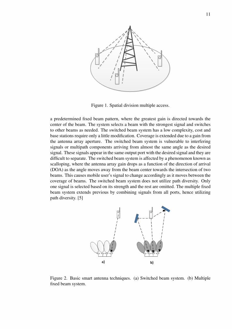
Transmitted signals can be separated from each other in time, frequency, code andspace. Divisions based on time, frequency and code have been widely studied andonly space-division multiple access (SDMA) remains to be exploited for future capac-ity improvements [3]. In SDMA, spectrally and temporally overlapping signals fromdifferent origin can be filtered in the spatial domain (Figure 1) [4]. SDMA can befurther subdivided into different methods: sectorization, switched beam systems, fixedmultiple beam systems, adaptive arrays and multiple input multiple output (MIMO)techniques.

An adaptive array is also known as a smart antenna. In this thesis, an adaptivearray refers to an array of antennas, which are controlled adaptively. A smart antenna,although being a synonym for adaptive array, will refer to a wider set of antennas, thatadaptive array is a part of.

Sectorization has been the most commonly used spatial technique in mobile commu-nication systems for years in an attempt to reduce interference and increase capacity.Cells are divided into three or six sectors, for example. Each sector is equipped witha dedicated antenna and radio frequency (RF) path. By increasing the amount of sec-torization, interference that is seen by the desired signal can be reduced. At the sametime, efficiency decreases because antenna patterns overlap more. Another drawbackis the increased number of handoffs for mobile users travelling within a cell as thesector count is increased. [5]

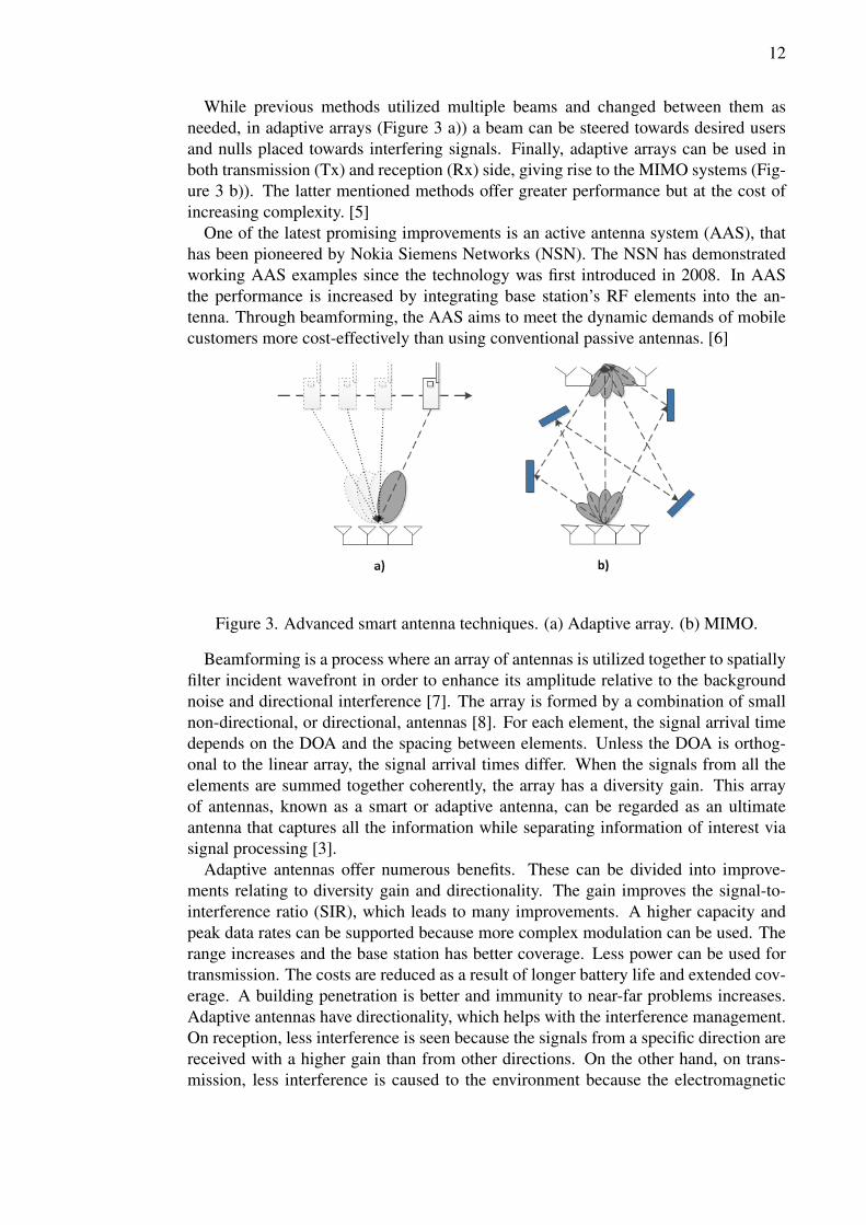
Early smart antenna types include the switched beam (Figure 2 a)) and multiple fixedbeam systems (Figure 2 b)). The switched beam method extends the sectorization.Macro-sectors are further divided into several micro sectors. Each micro sector has

11

Figure 1. Spatial division multiple access.

a predetermined fixed beam pattern, where the greatest gain is directed towards thecenter of the beam. The system selects a beam with the strongest signal and switchesto other beams as needed. The switched beam system has a low complexity, cost andbase stations require only a little modification. Coverage is extended due to a gain fromthe antenna array aperture. The switched beam system is vulnerable to interferingsignals or multipath components arriving from almost the same angle as the desiredsignal. These signals appear in the same output port with the desired signal and they aredifficult to separate. The switched beam system is affected by a phenomenon known asscalloping, where the antenna array gain drops as a function of the direction of arrival(DOA) as the angle moves away from the beam center towards the intersection of twobeams. This causes mobile user’s signal to change accordingly as it moves between thecoverage of beams. The switched beam system does not utilize path diversity. Onlyone signal is selected based on its strength and the rest are omitted. The multiple fixedbeam system extends previous by combining signals from all ports, hence utilizingpath diversity. [5]

Figure 2. Basic smart antenna techniques. (a) Switched beam system. (b) Multiplefixed beam system.

12

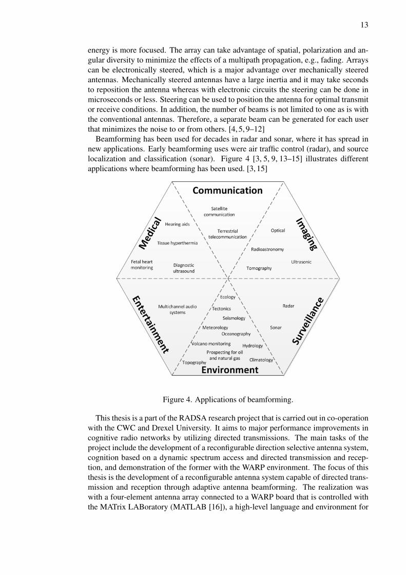
While previous methods utilized multiple beams and changed between them asneeded, in adaptive arrays (Figure 3 a)) a beam can be steered towards desired usersand nulls placed towards interfering signals. Finally, adaptive arrays can be used inboth transmission (Tx) and reception (Rx) side, giving rise to the MIMO systems (Fig-ure 3 b)). The latter mentioned methods offer greater performance but at the cost ofincreasing complexity. [5]

One of the latest promising improvements is an active antenna system (AAS), thathas been pioneered by Nokia Siemens Networks (NSN). The NSN has demonstratedworking AAS examples since the technology was first introduced in 2008. In AASthe performance is increased by integrating base station’s RF elements into the an-tenna. Through beamforming, the AAS aims to meet the dynamic demands of mobilecustomers more cost-effectively than using conventional passive antennas. [6]

Figure 3. Advanced smart antenna techniques. (a) Adaptive array. (b) MIMO.

Beamforming is a process where an array of antennas is utilized together to spatiallyfilter incident wavefront in order to enhance its amplitude relative to the backgroundnoise and directional interference [7]. The array is formed by a combination of smallnon-directional, or directional, antennas [8]. For each element, the signal arrival timedepends on the DOA and the spacing between elements. Unless the DOA is orthog-onal to the linear array, the signal arrival times differ. When the signals from all theelements are summed together coherently, the array has a diversity gain. This arrayof antennas, known as a smart or adaptive antenna, can be regarded as an ultimateantenna that captures all the information while separating information of interest viasignal processing [3].

Adaptive antennas offer numerous benefits. These can be divided into improve-ments relating to diversity gain and directionality. The gain improves the signal-to-interference ratio (SIR), which leads to many improvements. A higher capacity andpeak data rates can be supported because more complex modulation can be used. Therange increases and the base station has better coverage. Less power can be used fortransmission. The costs are reduced as a result of longer battery life and extended cov-erage. A building penetration is better and immunity to near-far problems increases.Adaptive antennas have directionality, which helps with the interference management.On reception, less interference is seen because the signals from a specific direction arereceived with a higher gain than from other directions. On the other hand, on trans-mission, less interference is caused to the environment because the electromagnetic

13

energy is more focused. The array can take advantage of spatial, polarization and an-gular diversity to minimize the effects of a multipath propagation, e.g., fading. Arrayscan be electronically steered, which is a major advantage over mechanically steeredantennas. Mechanically steered antennas have a large inertia and it may take secondsto reposition the antenna whereas with electronic circuits the steering can be done inmicroseconds or less. Steering can be used to position the antenna for optimal transmitor receive conditions. In addition, the number of beams is not limited to one as is withthe conventional antennas. Therefore, a separate beam can be generated for each userthat minimizes the noise to or from others. [4, 5, 9–12]

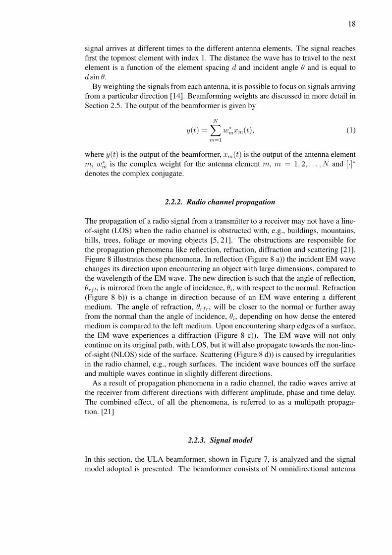
Beamforming has been used for decades in radar and sonar, where it has spread innew applications. Early beamforming uses were air traffic control (radar), and sourcelocalization and classification (sonar). Figure 4 [3, 5, 9, 13–15] illustrates differentapplications where beamforming has been used. [3, 15]

Figure 4. Applications of beamforming.

This thesis is a part of the RADSA research project that is carried out in co-operationwith the CWC and Drexel University. It aims to major performance improvements incognitive radio networks by utilizing directed transmissions. The main tasks of theproject include the development of a reconfigurable direction selective antenna system,cognition based on a dynamic spectrum access and directed transmission and recep-tion, and demonstration of the former with the WARP environment. The focus of thisthesis is the development of a reconfigurable antenna system capable of directed trans-mission and reception through adaptive antenna beamforming. The realization waswith a four-element antenna array connected to a WARP board that is controlled withthe MATrix LABoratory (MATLAB [16]), a high-level language and environment for

14

numerical computation, visualization and programming. The implementation utilizedthe channel 14 (2484 MHz) of the 2.4 GHz industrial, scientific and medical (ISM)band.

The outline of this thesis is as follows. Chapter 2 illustrates the beamforming con-cept in detail and the beamforming methods used in the implementation. In Chapter 3,the WARP board is introduced. Description of the calibration can be found in Chapter4. Measurements are presented in Chapter 5. Finally, a discussion and summary aregiven in Chapters 6 and 7, respectively.

15

2. BEAMFORMING

Beamforming, along with many other technologies, has evolved from an analog to adigital format. Performing beamforming in a digital domain rather than analogicallyat RF or intermediate frequency (IF) introduces many benefits. Digital beamforming(DBF) allows the control of the antenna array’s radiation pattern accurately at highclock frequencies. The beam’s direction and shape can be changed fast. Rapid re-configurability enables the implementation of adaptive algorithms, beam scanning andself-calibration. Generation of multiple simultaneous beams, that may overlap, is pos-sible with DBF. Multiple beams can be used, for example, in multipath discrimination.In analog beamforming, the propagation time differences between array elements arecompensated with time delays whereas in DBF it can be accomplished by controllingthe amplitudes and phases. [4, 9, 13, 17]

A conventional beamformer uses a single parabolic dish antenna (Figure 5 a)) andis capable of producing a single beam. It amplifies signals from the direction it ispointed at and attenuates those from other directions. For high spatial discrimina-tion, the aperture needs to be large in terms of wavelength. Mechanical operation fordirection selection limits the number of trackable signals to one and the change of di-rection is slow due to a physical repositioning of the dish. Furthermore, the response isfixed. These restraints and the increase in requirements have lead to the developmentof adaptive arrays, also known as phased arrays (Figure 5 b)). In a phased array, thedirection of focus is controlled by weighting the outputs of the array antennas. WithDBF, the direction is easily changed fast and multiple beams can be generated. Thephased array can remain stationary as the listening direction is almost independent ofthe orientation of the array. A phased array’s response can be adaptively changed,e.g., to combat emerging strong interference. Phased arrays are preferred over the con-ventional dish antennas because they require less space. A phased array’s maximumazimuth coverage is usually ±60◦ and multiple arrays can be combined to fulfill thecoverage requirements. However, phased arrays are not without their downsides. Theshape of the resulting beam varies as a function of the direction which it is pointingat. Its bandwidth is narrower than a conventional beamformer’s. Also, the design andmanufacturing are more expensive. [13, 14, 18]

Figure 5. Antennas for beamforming. (a) Parabolic dish antenna. (b) Phased array.

16

A single antenna can separate signals using time, frequency or code information.If two or more signals share the same attributes, for example they are using the samefrequency, and arrive at the antenna at the same time, the antenna is unable to decidethem apart. If the receiver uses more than one antenna, it can take advantage of spatialinformation. For the same scenario as before, incoming signals may share the sameattributes but if they arrive from different directions, they can be differentiated becausethey arrive at different antennas at different times. An adaptive antenna is formedby combining the information from multiple antennas together. This combination ofantennas is called an array and it can take many shapes.

This Chapter provides understanding about the beamforming. In Section 2.1, a coor-dinate system is defined that forms the basis for beamforming. Section 2.2 introducesthe principle of beamforming. Issues relating implementation are discussed in Sec-tion 2.3. The performance of beamformer is affected by several factors and these areconsidered in Section 2.4. Finally, beamforming techniques used in this thesis areintroduced in Section 2.5.

2.1. Coordinate system

The most commonly known coordinate system is a Cartesian system, which specifiesthe location in space with three coordinates, i.e., (x, y, z). In the context of antennas,it is not intuitive and a better alternative is to use a spherical coordinate system. Thespherical coordinates are also specified with three variables, i.e., (r, φ, θ), where r isthe radial distance, or range, from origin, φ is the azimuth angle and θ is the elevation,or more commonly known as a polar or zenith angle. Figure 6 relates these coordinatesystems.

Figure 6. Relation between the Cartesian and the spherical coordinate system.

17

2.2. Operating principle

Electromagnetic (EM) signals are generated by the moving charged particles. As thename suggests, it consists of two parts: an electric and magnetic component. Thesecomponents oscillate perpendicular to each other and in the direction of propagation.A signal propagates as an EM wave through medium such as air, water or vacuum.In a vacuum, wave travels with the speed of light. EM radiation induces a voltage tothe receiving antenna. A transmitting antenna operates in reverse by causing an EMradiation as a result of applied voltage.

2.2.1. Fundamentals

Beamforming is based on the wave behavior of EM waves. The waves interact witheach other through interference that may be either constructive or destructive. In beam-forming, the waves are combined constructively on some angles while for other anglesthey combine destructively [19]. Figure 7 depicts the principle of beamforming for auniform linear array (ULA).

Figure 7. Beamforming principle with a uniform linear array.

The signal impinges on the array from an angle θ relative to the broadside, whichis the direction perpendicular to the array. The signal is an EM wave that arrives asa wavefront, assuming the array is in the far-field of the radiating source. The arrayhas N elements and they are spaced distance d apart. Each of the elements samplethe incident EM wave, that is a spatiotemporal signal, and convert it to a temporalsignal [20]. Because the DOA of the signal is different from that of the broadside, the

18

signal arrives at different times to the different antenna elements. The signal reachesfirst the topmost element with index 1. The distance the wave has to travel to the nextelement is a function of the element spacing d and incident angle θ and is equal tod sin θ.

By weighting the signals from each antenna, it is possible to focus on signals arrivingfrom a particular direction [14]. Beamforming weights are discussed in more detail inSection 2.5. The output of the beamformer is given by

y(t) =N∑m=1

w∗mxm(t), (1)

where y(t) is the output of the beamformer, xm(t) is the output of the antenna elementm, w∗m is the complex weight for the antenna element m, m = 1, 2, . . . , N and [·]∗denotes the complex conjugate.

2.2.2. Radio channel propagation

The propagation of a radio signal from a transmitter to a receiver may not have a line-of-sight (LOS) when the radio channel is obstructed with, e.g., buildings, mountains,hills, trees, foliage or moving objects [5, 21]. The obstructions are responsible forthe propagation phenomena like reflection, refraction, diffraction and scattering [21].Figure 8 illustrates these phenomena. In reflection (Figure 8 a)) the incident EM wavechanges its direction upon encountering an object with large dimensions, compared tothe wavelength of the EM wave. The new direction is such that the angle of reflection,θrfl, is mirrored from the angle of incidence, θi, with respect to the normal. Refraction(Figure 8 b)) is a change in direction because of an EM wave entering a differentmedium. The angle of refraction, θrfr, will be closer to the normal or further awayfrom the normal than the angle of incidence, θi, depending on how dense the enteredmedium is compared to the left medium. Upon encountering sharp edges of a surface,the EM wave experiences a diffraction (Figure 8 c)). The EM wave will not onlycontinue on its original path, with LOS, but it will also propagate towards the non-line-of-sight (NLOS) side of the surface. Scattering (Figure 8 d)) is caused by irregularitiesin the radio channel, e.g., rough surfaces. The incident wave bounces off the surfaceand multiple waves continue in slightly different directions.

As a result of propagation phenomena in a radio channel, the radio waves arrive atthe receiver from different directions with different amplitude, phase and time delay.The combined effect, of all the phenomena, is referred to as a multipath propaga-tion. [21]

2.2.3. Signal model

In this section, the ULA beamformer, shown in Figure 7, is analyzed and the signalmodel adopted is presented. The beamformer consists of N omnidirectional antenna

19

Figure 8. Radio propagation phenomena. (a) Reflection. (b) Refraction. (c) Diffrac-tion. (d) Scattering.

elements spaced distance d apart. The propagation delay τm(θ) for an impinging signalfrom the first antenna to the mth, with DOA of θ, is

τm(θ) =(m− 1)d sin θ

c, (2)

where θ is the incident angle, θ ∈ [−π/2 π/2] and c is the speed of light [22].The impinging signal is assumed to be a complex plane wave of the form

si(t)ejωt, (3)

where si(t) is the ith signal and ω is the angular frequency.The wavefront arrives at the mth element τm(θ) seconds later than at the first ele-

ment. Hence the signal induced on the mth element due to the ith source is expressedas

si(t)ejω(t−τm(θi)). (4)

20

The total signal, xm(t), induced due to all M sources and noise on the mth element, isgiven by

xm(t) =M∑i=1

si(t)ejω(t−τm(θi)) + nm(t), (5)

where nm(t) is the noise at themth element. The noise is assumed to be white Gaussiannoise with variance equal to σ2

n. The noise at different antenna elements is indepen-dent. [23]

The output of the beamformer given in (1) can be written in vector format as

y(t) = wHx(t), (6)

where [·]H denotes the Hermitian (complex conjugate) transpose, w is the weight vec-tor, with N complex coefficients, of the array given as

w = [w1 w2 . . . wN ]T , (7)

where [·]T denotes the transpose and x is the vector of signals induced on all the ele-ments as

x(t) = [x1(t) x2(t) . . . xN(t)]T . (8)

Throughout this thesis, vectors and matrices are denoted with boldface lowercase anduppercase letters, respectively. [22, 23]

Assuming the elements of x(t) are zero mean stationary processes, the mean outputpower of the beamformer is

P (w) = E{y(t)yH(t)} = wHRw, (9)

where E{·} denotes the expectation operator and R is the array correlation matrixdefined as

R = E{x(t)xH(t)}. (10)

Through algebraic manipulation of (5), (8) and (10), the correlation matrix, R, can bewritten as

R =M−1∑i=0

piai(ω)aHi (ω) + σ2nI, (11)

where pi denotes the power of the ith source measured at one of the elements of thearray, ai(ω) is the steering vector for ith source and I denotes an identity matrix. Thecorrelation matrix can be expressed in a matrix notation as

R = ASAH + σ2nI, (12)

where matrix A consists of steering vectors as

A = [a0(ω) a1(ω) . . . aM−1(ω)] (13)

and S is the source correlation matrix. [23]The steering vector ai(ω) is given by

ai(ω) = [1 e−jωτ2(θ) . . . e−jωτN (θ)]T . (14)

21

The steering vector ai(ω) can also be expressed in another form by substituting ω with2πf and (2) into (14). This yields

ωτm(θ) = 2πf(m− 1)d sin θ

c= k(m− 1)d sin θ, (15)

where k is the wave number, given as

k =2π

λ, (16)

where λ is the wavelength. Finally, the steering vector can be written as

a(θi) = [1 e−jkd sin θi e−jk2d sin θi . . . e−jk(N−1)d sin θi ]T (17)

[22].The weight vector, w, is a function of the steering vector(s) and is further discussed

in Section 2.5. The steering vector depends on the incident angle, θ, as in (17). There-fore, the mean output power, P (w), in (9) can be written as

P (θ) = wH(θ)RwH(θ). (18)

Radiation pattern (RP), also beam pattern, can be given in dB as

RP = 20 log10

|P (θ)|max |P (θ)|

(19)

[23].

2.2.4. Assumptions

The preceding analysis assumes some simplifying assumptions. However, the analysiscan be utilized in less ideal environments, such as obstructed multipath environments,with some error introduced. The medium is lossless in a sense that it does not attenu-ate the propagating signal further than predicted by the wave equation, i.e., the signalis attenuated only inversely proportionally to the distance squared. In addition, thepropagation speed is uniform. The medium is also nondispersive , i.e., it has no fre-quency dependency to the wave propagation. A point source is assumed to generatethe propagating signal. That implies that the size of the source is small with respect tothe distance between the source and antennas receiving the signal. A source produceswaves that are spherical around it, however, when the antenna array is in the far-field(large distance away) of the source, these spherical waves can be approximated withplane waves. As previously discussed, the propagation delays between array elementsare compensated with phase shifts. This is known as the narrowband assumption wherethe bandwidth of a signal is small in comparison with the carrier frequency. Thermalnoise is assumed to be uncorrelated for all the array elements, as well as betweenthem. Each element in the array has an equal, omnidirectional response. Locations ofthe array elements are assumed to be known perfectly as they are needed for properdelay computations. The array elements are spaced close enough so there is no am-plitude variation between the signals received due to the attenuation predicted by thewave equation. No mutual coupling exists between elements. The number of signalsimpinging the array is finite, i.e., all the incoming signals can be decomposed into adiscrete number of plane waves. [12, 14, 24, 25]

22

2.3. Implementation issues

2.3.1. Array geometry

Phased arrays can be formed with varying geometries. In general, they can be clas-sified based on the number of dimensions they extend to: linear (one-dimensional),planar (two-dimensional), with geometries such as circular, rectangular and hexago-nal, for example, and volumetric (three-dimensional). The elements can be spacedregularly or irregularly (randomly). Regular spacing is further subdivided into uni-form and nonuniform. Phased arrays are usually arranged as a ULA, uniform circulararray (UCA) or planar arrays of elements with the same polarization, low gain andorientation. Uniform arrays, while being simple, have redundant information that isavoided in minimum/null redundancy arrays (MRA/NRA). In MRA/NRA, the objec-tive is to maximize the spatial resolution and number of spacings for the given numberof elements. As an example, let us assume a four-element linear array (Figure 9 a)) isplaced on the x-axis. Its elements are located at coordinates 0, 1, 2 and 3. There arethree different spacings (Figure 9 b)), where spacing denotes the relative distance be-tween elements. A spacing with distance 1 is between elements in locations 0 and 1, inlocations 1 and 2, and in locations 2 and 3. The second spacing, with distance 2, existsbetween elements in locations 0 and 2 and in locations 1 and 3. Finally, the spacingwith distance 3 exists between elements in locations 0 and 3. For each spacing, a singleoccurrence is enough and additional ones introduce redundancy, as is with spacings ofdistance 1 and 2. An array with equal length can be implemented as a NRA with threeelements (Figure 9 c)) by placing them in coordinates 0, 1 and 3. In this configuration,there are 3 different spacings with distances (Figure 9 d)): 1 (between locations 0 and1), 2 (between locations 1 and 3) and 3 (between locations 0 and 3). Each spacing ex-ists only once and there is no redundancy. The downside of MRAs/NRAs is, that theirspacings are difficult to compute, when the number of elements is high. Conversely,when the number of elements is low, the sidelobe levels are high. [3, 12, 13, 26, 27]

2.3.2. Pattern multiplication

The total radiation pattern of an antenna array is the product of the element patternand the array factor (AF). This is known as a pattern multiplication. The elementpattern is dependent on the physical dimensions and EM characteristics of the radiatingelement. AF depends on the amplitude, phase and position of each element in thearray. Arrays can be designed without knowledge of the used antennas as a result ofpattern multiplication. Pattern multiplication can also be used to determine the AF ofa complicated array. A rectangular array, for example, can be considered as a lineararray consisting of linear arrays. [3, 5, 9]

2.4. Performance impacting factors

A measure of the beamforming performance is a radiation pattern that depicts the gainof an adaptive array as a function of angle. In this section, the beamforming perfor-

23

Figure 9. Uniform linear array vs. null redundancy array. (a) ULA of length 4. (b)Spatial sensitivity of the ULA. (c) NRA of length 4. (d) Spatial sensitivity of the NRA.

mance is illustrated as an array factor and the contribution of element pattern is notconsidered. The gain is dependent on the aperture of the array, through the numberof elements and their spacings, beam’s scan angle and the illumination. The perfor-mance is also measured as a beamwidth of the main beam where most of the energyis focused. Two common beamwidths are null-to-null beamwidth (NNBW) and 3 dB,also half power, beamwidth [5]. These are illustrated in Figure 10. In the followingsections, each of these factors will be discussed separately for equispaced arrays.

2.4.1. Number of elements

The AF of an adaptive array can be controlled with the number of elements. Generally,the more elements it has, the better the performance. Figures 11 and 12 show the AFsfor the arrays with 4, 8, 16 and 32 elements.

By increasing the number of elements, the AF has more sidelobes but their levels arelower. This improves directionality and interference is cancelled more effectively. Thenumber of nulls is increased and they are deeper. The beams are narrower and the gainof the array is higher because of spatial diversity. The number of elements possible isconstrained by a cost and physical limitations, e.g., if the array were to be mounted onan aircraft, there would an upper limit to its size. [5, 11, 12, 28]

24

Figure 10. Null-to-null beamwidth and 3-dB beamwidth in a radiation pattern.

Figure 11. The array factors for 4 and 8 element arrays. Elements are spaced 0.5λapart.

25

Figure 12. The array factors for 16 and 32 element arrays. Elements are spaced 0.5λapart.

2.4.2. Element spacing

Element spacing, along with the number of elements, determines the aperture for thearray. As discussed in the previous section, a larger aperture is desirable. As the spac-ing is increased, sidelobes, with equal gain to the main beam, appear. These are calledgrating lobes and their locations are periodic relative to the inverse of element spac-ing. In reception, the grating lobes cause directional ambiguity because the signalsmay come from the direction of the main beam or the grating lobe and result in thesame response. In transmission, the transmitted power is wasted towards grating lobesbecause the receiver is on the direction of the main beam. In addition, the power trans-mitted towards grating lobes causes a high interference to the other users. Therefore,grating lobes are usually avoided, although they can be beneficial in some cases suchas transmit diversity. [5, 9, 11, 13, 28]

The grating lobes can be prevented by reducing the element spacing. However, asthe elements are closer to each other, their mutual coupling increases. In order to keepthe aperture the same, to retain its properties, the number of elements needs to beincreased to compensate for reduced element spacing. More elements lead to a highercost. Hence, there is a tradeoff for choosing the element spacing. Figures 13 and 14demonstrate the effect of the element spacing and the existence of the grating lobes.The arrays share the same aperture of 4λ but differ in the element spacing. Shorterspacings are compensated with more elements to match the aperture requirements. [9]

The existence of grating lobes is explained as a spatial aliasing that is similar to atemporal aliasing. In an analog-to-digital converter (ADC), the continuous-time signalis sampled to convert it into a discrete-time signal. Temporal aliasing occurs when thesignal is sampled at a lower rate than the Nyquist sampling rate, so that two signalswith different frequencies could yield the same discrete-time signal. In phased arrays,the antennas sample the impinging signals spatially. If the antennas are spaced too

26

Figure 13. The array factors for arrays with element spacing of 0.25 λ and 0.5 λ. Theaperture is 4λ for both arrays. No grating lobes present.

Figure 14. The array factors for arrays with element spacing of λ and 2λ. The apertureis 4λ for both arrays. Grating lobes are present in both cases: two for λ spacing andfour for 2λ spacing.

27

far apart, the signals will not be sampled densely enough. The sources at differentdirections will have the same steering vector and this ambiguity in the DOAs of thesources is known as the spatial aliasing. [22]

Spatial oversampling, i.e., the spacing is less than half the wavelength, does not im-prove the beamformer’s performance in terms of resolution. Spatial undersampling,i.e., the spacing is larger than half the wavelength, causes grating lobes. Thus, thespacing is usually chosen to be half the wavelength to maximize the aperture, yet toplace grating lobes at the horizon, where they cause no harm. A uniform spacing hassidelobe level limits of -13 dB and -18 dB for the first and second sidelobes, respec-tively. The more the antenna array has elements, the lower the sidelobe levels are. Toreduce the sidelobe levels, a non-uniform spacing can be used but with a tradeoff ofincreasing beamwidth. [13, 14]

As the element spacing is measured relative to the wavelength, it is dependent of thefrequency. Signals with different frequencies experience the fixed spacing differently.In this thesis, narrowband systems are discussed and for wideband systems the issueneeds to be addressed accordingly.

2.4.3. Scan angle

For phased arrays, the direction of the main beam, i.e., the scan angle, can be controlledwith the weighting vector. As the scan angle increases the beamwidth broadens. Theincreased beamwidth results in a degraded performance and hence the maximum scanangle rarely exceeds ±60◦. The beamwidth broadening is slower for arrays with alarger aperture. Figures 15 and 16 depict the beamwidth broadening for scan angles0◦, 15◦, 30◦ and 45◦ with aperture size of 4λ. Figures 17 and 18 show the same but forthe aperture size of 10λ. [13, 17, 29]

Figure 15. The array factors for an array that is scanned to angles 0◦ and 15◦. Apertureis 4λ.

28



29


2.4.4. Amplitude illumination

The amplitude illumination, the input to the antenna element, is usually constant. Thesidelobe that is closest to the main beam has a level of around -13 dB (Figures 19 and20, constant illumination). The sidelobe levels can be reduced by using an amplitudetaper. Tapering is accomplished by controlling the amplitude illumination. The illu-mination for the element is reduced while moving away from the center of the array.Figures 19 and 20 illustrate the use of a taper for an array with 4 and 16 elements,respectively. [9, 13, 29]

Tapering produces constant sidelobe levels, where the level can be specified [11].Lowering the sidelobe levels broadens the main beam. Beam broadening is propor-tional to the number of elements in the array. The less elements in the array, the largerthe beam broadening is. For this reason, tapering is not usually used when the numberof elements in the array is low, e.g., less than 16. The gain of the main beam no longerremains at 0 dB, but is reduced. The gain reduction is visible in RP, but not in AF. [14].

2.5. Techniques

The beamforming techniques differ in how they compute the weights and how theyare applied. Computation of the weights is either non-adaptive or adaptive. Non-adaptive techniques are independent of the input data and hence suboptimal. Adaptivetechniques use the a priori statistics of the data and change, or adapt, in response to thedata received to derive the optimal weights. [5, 14]

Adaptive techniques use a criterion function that will optimize the spatial responseof the beamformer for a maximum communication channel quality. The criterion isselected to enhance the desired signal and to minimize the contribution of interferingsignals. Some commonly used criteria include minimum mean square error (MMSE),

30

Figure 19. The array factors for an array with 4 elements. Amplitude illumination isvaried between constant, -20 dB taper and -30 dB taper. Dolph-Chebyshev taper isused.

Figure 20. The array factors for an array with 16 elements. Amplitude illuminationis varied between constant, -20 dB taper and -30 dB taper. Dolph-Chebyshev taper isused.

31

maximum SIR and minimum variance. As adaptive techniques rely on the statisticsof the data, they can be classified as statistically optimal, adaptive and partially adap-tive. The statistically optimal chooses the weights based on the statistics of the data.The statistics of the data are not usually known and they need to be estimated. Anadaptive technique can use two methods for estimation. First is the block adaptationwhere statistics are estimated from a temporal block of array data and used to derivethe optimal weights. Secondly, a continuous adaptation can be used, where the weightsare constantly adjusted as new data arrives. The resulting weight vector sequence con-verges to the optimal vector. A partially adaptive uses a subset of degrees of freedomthat yields a minimal loss in performance. The amount of computation is decreasedand the adaptation is faster. [8, 15]

Beamforming can be implemented in two ways depending on how the weights areapplied. In element-space beamforming, the weights are applied directly to the outputsof the antenna elements. For the beam-space beamformer, the outputs of antenna ele-ments are fed into a multiple-beam beamformer to yield the orthogonal beams. Eachoutput of the beamformer is weighted, i.e., the beams themselves. Only non-adaptiveelement-space beamforming techniques will be further discussed because only they areimplemented. [20]

2.5.1. Conventional

The conventional beamforming is the simplest beamformer. It is also known asthe classical beamformer, the delay-and-sum beamformer, the beam steering and theBartlett’s method. Steering of the beam is achieved by applying amplitudes and phasesthat compensate the propagation differences between the array elements and determinethe look direction. Ideally, in an ULA the weights have equal magnitude and are givenby

wC =1

Na(θ0), (20)

where N is the number of elements, a(θ0) is the steering vector and θ0 is the incidentangle of the desired signal. [5, 30]

It is assumed that only one signal source exists, with power ps. It is located at thelook direction θ0. The signal induced on the mth element due to this source alone is

xms(t) = si(t)ejω0(t−τm(θ0). (21)

Using vector notation and equation (14), it can be written that the signal induced on allthe elements due to this source alone is

xs(t) = si(t)ejω0ta(θ0). (22)

The beamformer output with the weight vector wC is

y(t) = wHC xs(t) = si(t)e

jω0t, (23)

resulting in the mean output power to be

P (ωC) = E{y(t) y∗(t)} = ps, (24)

32

which is equal to the source power. [23]The conventional beamformer maximizes the signal-to-noise ratio (SNR) under spe-

cial circumstances: the noise is uncorrelated and no directional interference is present.With uncorrelated noise, the noise correlation matrix is

RN = σ2nI (25)

and the beamformer output noise power is

PN = wHCRNwC =

σ2n

N. (26)

Noise power at the beamformer output is N times less than at a single element. Hence,the uncorrelated noise is reduced by N times and the beamformer output SNR is

SNRout = psN

σ2n

. (27)

Since the input SNR isSNRin =

psσ2n

, (28)

the array has a gain of N . Thus, the gain of the array is directly proportional to thenumber of elements N , and improvements in gain, and in SNR, can be achieved withlarger arrays. While conventional beamformer yields maximum output SNR with nodirectional interference, it will not be effective if such an interference is present. Theresponse of the beamformer towards an interference source in a direction of θ1 is

wHC a(θ1) =

1

NaH(θ0)a(θ1), (29)

where a(θ0) denotes the steering vector of a desired source and a(θ1) that of an inter-ferer. [23]

The main beam’s beamwidth determines the resolution of the array, sources that arelocated closer than the beamwidth will not be resolved [27].

2.5.2. Null-steering

As in the conventional beamformer, the maximum gain is directed towards the desiredsignal. Additionally, minimum gains (nulls) are placed towards interfering signals tosuppress them. An array with N elements is capable of producing N − 1 nulls andtherefore N − 1 interfering sources can be eliminated. However, the DOAs of thedesired signal and the interfering sources must be known. [5, 23, 30]

Null-steering beamforming can be formulated as

wHNSA = wH

NS[a(θ0) a(θ1) . . . a(θN−1)] = [1 0 · · · 0], (30)

where wHNS is the weighting vector, A is the steering matrix, a(θ0) is the steering vector

for the desired signal and a(θi) is the steering vector for the interfering signal i, wherei = 1, 2, . . . , N − 1. The desired signal is given a unity response and the interfering

33

signals have a zero response. The solution is straightforward if A is non-singular, i.e.,A is a square matrix and all the steering vectors a(θi), i = 1, 2, . . . , N −1, are linearlyindependent. Under these conditions, it results that the weighting vector is

wHNS = [1 0 · · · 0]A−1, (31)

where [·]−1 denotes the matrix inversion. [5, 23]If the number of required nulls is less than N − 1 (A is not a square matrix), A is

singular. Then, a solution can be found using a pseudo inverse, i.e.,

wHNS = [1 0 · · · 0]A+, (32)

where A+ denotes the pseudo inverse of A defined as

A+ = AH(AAH)−1. [23] (33)

Although the interfering signals are eliminated, or at least reduced, the null-steeringbeamformer does not minimize the uncorrelated noise. The uncorrelated noise can beminimized by choosing weights that minimize the mean output power in addition tothe aforementioned constraints. [23]

In the Figures 21 through 24, the conventional and null-steering beamformers arecompared for the source directions of 0◦ and 15◦, and interference directions of −20◦

and −40◦. The emphasis on these two techniques is different in terms of receiving thesource signal. In conventional beamforming, the main beam, with maximum gain, issteered towards the target. It does not consider interfering sources. On the other hand,the null-steering beamformer focuses on suppressing the interfering sources. While itdoes also steer the main beam, its performance might be sacrificed if a null is locatedtoo close to the source direction.

Figure 21. Conventional vs. null-steering beamforming. Source direction is 0◦ andinterference direction is −20◦.

34



35


36

3. WIRELESS OPEN-ACCESS RESEARCH PLATFORM

The WARP board is a wireless network research platform developed at the Rice Uni-versity. It has been built around Xilinx’s Virtex-II Pro FPGA. The WARP offers aplatform which allows the user to modify both hardware and software. The Rice Uni-versity provides a reference design for the WARP that enables researches to focus ona specific area instead of requiring them to design a complete solution. This facilitatesa fast prototyping of new wireless networks. Since WARP’s launch in 2005, it hasgained increasing interest among researches worldwide. It has resulted in more than75 publications [31] and is in use in more than 100 research groups in 24 countries.In 2012, the WARP users released 38 new papers and WARP papers were cited 84times. [32]

3.1. FPGA board

A version 1 WARP FPGA board was used in this thesis and is shown in Figure 25 [33].The core of the board is the aforementioned Xilinx Virtex-II Pro XC2VP70 FPGA. TheFPGA has 5.9 Mb RAM and logic slices can be used for extra 1034 kb of additionalmemory. There are two banks of 18 Mb pipelined ZBT SRAM on the FPGA board.The FPGA is surrounded by four identical daughtercard slots. Below the FPGA is aslot for the clock board. [34]

The FPGA board includes several I/O devices: five push buttons, 4-position DIP-switch, four LEDs and two 7-segment displays. 10/100 Mbps Ethernet is located atthe upper right corner. Other I/O include RS-232 UART and 16-bits of unbuffered3.3V I/O connected directly to the FPGA I/O pins. The Virtex-II Pro FPGA has 8multi-gigabit transceivers (MGT). Each MGT is a full-duplex transceiver supportingdata rates up to 3.125 Gbps. The MGTs are located at the top of FPGA board. [34]

3.2. FPGA

Virtex-II family’s XC2VP70FF1517-6C is a high-performance platform FPGA. Its re-sources include [35]:

• 33k logic slices

• 328 18x18 bit multiplier blocks

• 328 Block RAMs

• 2 PowerPC cores

The FPGA can be configured with the on-board USB configuration circuit, externalJTAG cable and SystemAce CompactFlash (CF) chip. The SystemAce chip is a ver-satile configuration option as up to eight configurations can be stored on the CF card.The configuration is loaded automatically on power-up or via the manual reset button.The configuration is selected with a DIP switch. [34]

37

Figure 25. WARP FPGA board.

3.3. Radio board

Four available daughtercard slots on the WARP FPGA board can be equipped withradio boards. The radio board (Figure 26 [36]) provides the WARP its radio commu-nication capabilities. The radio board’s RF section consists of Maxim’s MAX2829dual-band transceiver, power amplifier and two antenna ports. Figure 27 illustrates thearchitecture of the radio board [36]. The key features of the transceiver are: [34]

• Dual-band (2400-2500 MHz, 4900-5875 MHz)

• Up to 40 MHz bandwidth

• Analog I/Q Tx and Rx interfaces

• 60 dB received signal strength indicator (RSSI) range

• 30 dB Tx power control range

• 93 dB Rx gain control range

• MIMO capable

The radio board can be controlled with two custom peripherals: a radio controllerand a radio bridge. The radio controller uses SPI logic to manipulate radio and digital-to-analog converter (DAC) chip registers. In addition, it tracks the control pins of both

38

Figure 26. Radio board.

Figure 27. Radio board architecture.

chips. The radio controller does not directly connect to the radio board, but utilizes theradio bridge as a proxy. The separation of control logic and connections to differentperipherals enables the use of a single controller to control all the radio boards. [34]

The WARP FGPA board can accommodate varying number of radio boards and assuch the radio boards have been designed to be modular. Each of the radio boards isequipped with its own phase-locked loop (PLL). The PLLs are not phase synchronizedto each other, which is a disadvantage in phased array designs. For beamforming, thephase differences need to be taken into account.

3.4. WARPLab

WARPLab is a framework combining WARP with MATLAB. WARP nodes are con-trolled directly from the MATLAB workspace. Signals to be transmitted are generatedin MATLAB and passed to WARP nodes via Ethernet links. Transmission is in real-

39

time over-the-air (OTA) with WARP nodes. Novel physical layer (PHY) implementa-tions can be implemented and tested quickly with the MATLAB M-code. [37]

WARP nodes and a PC running MATLAB are connected to a switch via Ethernetlinks. Up to 16 WARP nodes can be connected to a single PC. Figure 28 depicts theWARPLab architecture [37].

Figure 28. WARPLab architecture.

Ethernet links are used to transfer the data between a PC and WARP nodes. The datacan be signal samples or control information. [37]

Transmission samples are generated in MATLAB and transferred to transmittingWARP nodes’ buffers. A trigger is sent to both transmitting and receiving WARPnodes. The trigger commences transmission and reception simultaneously. The trans-mission and capture of samples happen in real-time OTA. Captured samples are storedinto buffers in receiving WARP nodes. The samples are transferred to a PC, wherethey are processed offline in MATLAB. [37]

A reference design for both the WARP nodes and MATLAB is provided by the RiceUniversity. The reference design for the FPGA provides functions such as Tx and Rxbuffers, radio controller, automatic gain control (AGC) and Ethernet MAC as FPGAlogic. The reference M-code enables the control and interaction with the WARP nodeson a PC. Both of these reference designs can be modified and extended as needed.WARPLab does not enable real-time sample processing since the samples need to betransferred between WARP nodes and a PC. The reference design for FPGA can bemodified if real-time functionality is required. Hence, WARPLab can be used forprototyping a design before it is implemented on the FPGA. [37]

40

4. CALIBRATION

So far, the discussion about beamforming has expected ideal conditions. In practice,this is rarely, if ever, the case. The adaptive array has to be calibrated to minimize theeffects of nonidealities.

Antenna element hardware and cables can introduce amplitude and phase mismatch[38–41]. The position of the antenna element or the signal DOA might be uncertain[38–40]. A close proximity of antenna elements causes mutual coupling, i.e., electro-magnetic interaction and increases with smaller inter-element spacing [38, 39, 41, 42].The metal of the tower, the antenna array is mounted on, can affect the radiation patternand is known as the tower effect [43].

The calibration can be performed using different techniques. Some techniques iso-late the error sources and compensate the effects one at a time while others handlemultiple error sources simultaneously. A common method is to place the transmitter ata known location relative to the antenna array. The response of the antenna array can becompared against the expected response of an ideal array. The difference can be usedas an estimate for the distortion experienced in the array. Finally, it can be compen-sated to yield a close to ideal array. In practice, a multipath propagation can introduceunknown distortion unless eliminated, for example, using an anechoic chamber formeasurements. Additionally, the transmitter needs to reside in the far-field of the arrayfor correct beamforming operation. Another common method is to inject a signal toall the array channels with an equal phase. The measured array outputs can be usedto estimate the amplitude and phase distortions. Other methods include using knownenvironmental reflectors, multiple scattering sources and blind techniques. [38, 39]

The calibration performed in this thesis comprises the calibration of the PLLs foundin each radio board on the WARP and the calibration of the antenna array that is knownas the array manifold measurement.

4.1. Phase-locked loop calibration

Implementing beamforming on the WARP board required additional calibration dueto its modular design. Each of the antenna array antennas was connected to its ownradio board with its own PLL. Each of the radio boards was driven by the same clockand they were frequency synchronized but not phase synchronized. As beamformingis based on controlling the amplitude and phase between different antennas, it is vitalthat any phase offsets among radio boards are compensated.

The PLLs lock with a random phase offset whenever WARP is powered on or thechannel is changed. The phase offset remains constant until the PLL locks again. Aphase synchronization was achieved by choosing one of the radio boards as a referenceand synchronizing others to it. Figure 29 demonstrates random phase offsets in PLLsand synchronization to reference.

Each of the PLLs has a random phase offset, αi, that is independent of the others.The PLL of radio board 1 was selected as the reference to whom others are synchro-nized to.

The PLLs were phase synchronized by pairing up radio boards and transmitting areference signal between them. The radio boards were connected to each other via

41

Figure 29. (a) Random phase offsets in the PLLs with respect to clock. (b) Referenceselection and synchronization.

a coaxial cable and an attenuator to remove the effect of the radio channel. Table 1depicts the phase offset measurement setups used in the phase synchronization.

The measurements are numbered as #X , whereX denotes the measurement number.For every measurement, there is a transmitter and receiver radio, denoted by numbersin Tx and Rx columns, respectively. Phase offsets are measured for radios 2, 3 and4 with respect to reference radio 1. Phase offset is an addition of two measurements,where a measurement indicated with + contributes as is and a measurement indicatedwith − contributes as complemented.

Figure 30 shows the phase offset measurement #1 setup.

Table 1. Phase offset measurement setups

Radio mode Phase offsetMeasurement Tx Rx 2 vs 1 3 vs 1 4 vs 1

#1 1 3 - -#2 2 3 +#3 4 3 +#4 3 4 +#5 1 4 -

In order to phase synchronize radio board 1 (reference) and radio board 2, two mea-surements (#1 and #2) were required. In measurement #1, the radio board 1 transmitted

42

Figure 30. PLL phase offset measurement #1 setup.

a reference signal to the radio board 3. The received signal’s phase at the radio board 3was compared against the known phase of the reference signal to determine the phaseshift from radio board 1 to 3. In measurement #2, the same operation was performedexcept now the radio board 2 was the transmitter. The phase offsets from measure-ments #2 and #1 were added together according to table 1, i.e., the phase offset frommeasurement #2 as is and the phase offset from measurement #1 as complemented. Fi-nally, the aforementioned addition yielded the phase offset for the PLL 2 with respectto the reference PLL 1. The phase offsets for the PLLs 3 and 4 with respect to thereference PLL 1 could be resolved with the same procedure utilizing measurements asshown in table 1.

Figure 31 details the pairwise measurements explained above. In Figure 31 a) andb), the phase offset between two radio boards is measured. The factors affecting themeasured phase offset are separated. On the transmitter side, the phase changes dueto the transmitter PLL in the upconversion stage, denoted as αi and αj in Figure 31 a)and b), respectively. On the receiver side, the phase changes due to a reverse operationin the downconversion stage and propagation delay. The phase offset in the downcon-version stage is denoted as αk in both Figure 31 a) and b). Its sign is a complementto that in upconversion stage because of reverse operation. The PLLs advance theirphases continuously and the receiver side PLL experiences a delay while the signalpropagates. As the signal arrives at the receiver PLL, after propagation, its phase is nolonger the same as it was during a reference point in the transmitter PLL. The changein phase is perceived erroneously as an additional phase offset denoted as δ.

Figure 32 illustrates the effect of propagation delay. The unit circles on the leftside represent the phases of PLLs while the signal is at the transmitter upconversionstage. The right side unit circles represent the phases of PLLs while the signal is atthe receiver downconversion stage. Both of the PLLs have their phases advanced byδ. The receiver side angle rotates in the opposite direction as the transmitter side angle

43

Figure 31. (a) Phase offset measurement between radio boards i (Tx) and k (Rx). (b)Phase offset measurement between radio boards j (Tx) and k (Rx). (c) Phase offset atradio board j relative to radio board i. (d) Phase compensation to match radio board jto reference radio board i.

44

Figure 32. The effect of propagation delay in phase offset measurement.

since the downconversion performs a reverse operation compared with the upconver-sion. The correct phase offset between the transmitter and receiver PLLs would bedetermined by comparing the phases at the same time instant. However, the signal isnot available for analysis until the end of path. Thus, the measurement yields, as thephase offset, the combined effect of all three factors. To eliminate the contribution ofunknown propagation delay to the phase offset, two measurements are performed. Themeasurements differ only in transmitting radio board. Hence, the phase offsets differonly with phase offset between different transmitters as is shown in Figure 31 c). Afterthe phase offset between two radio boards is known, their phases can be synchronizedby applying the complement of the phase offset (Figure 31 d)).

4.2. Array manifold measurement

The antenna array was calibrated by measuring its response for each DOA. The setof steering vectors, for each DOA, is known as the array manifold. The measurementwas performed in an anechoic chamber to avoid errors due to multipath componentsand interference. The purpose of the array manifold measurement was not to make theantenna array ideal by compensating the nonidealities. Instead, the acquired steeringvectors included the effects of nonidealities and were used to derive the beamformingweights. The beamforming weights took into account the effects of nonidealities.

Figure 33 represents the measurement configuration. On the transmitter side, a sin-gle omnidirectional antenna transmitted a reference signal. The transmitter antennawas positioned perpendicularly towards the antenna array’s center. The antenna array,consisting of four identical omnidirectional antennas, spaced half the wavelength apart,operated as the receiving side and was rotated 180◦ around its center. As the array wasrotated counterclockwise, the DOA of the transmitter signal changed and the array’sresponse was measured for each DOA. The array manifold was measured for DOAs inrange of [−90◦, 90◦] with 5◦ intervals as an average of 100 samples. Since the main

45

beam’s beamwidth is large for a four-element ULA, a 5◦ interval was chosen to resultin adequate precision. In Figures 34 and 35, the array manifold measurement in ananechoic chamber is represented from the point of view of the transmitter antenna andthe antenna array, respectively.

Figure 33. Array manifold measurement in an anechoic chamber. The antenna array(Rx) is at the starting position for the measurement. The DOA of the signal fromtransmitter is now −90◦. The antenna array is rotated 180◦ counterclockwise.

46

Figure 34. Array manifold measurement in an anechoic chamber from the point ofview of the transmitter antenna.

Figure 35. Array manifold measurement in an anechoic chamber from the point ofview of the antenna array. The used antenna array can be seen in this figure.

47

5. MEASUREMENTS

The WARPLab implementation of beamforming algorithms was evaluated by measur-ing the transmitted and received beamform of the antenna array for the DOA of 0◦.The measured radiation patterns were compared against the ideal ones. The measure-ments were performed in an anechoic chamber to eliminate the effects of multipathpropagation and interference.

Section 5.1 explains the setup used in the measurements. The receive and transmitbeamforming results, for both conventional and null-steering beamforming algorithms,are presented in Sections 5.2 and 5.3, respectively.

5.1. Measurement setup

The setup is equivalent to the array manifold measurement described in Section 4.2except now both the single omnidirectional antenna and the antenna array can oper-ate as a receiver and transmitter. In receive beamforming, the antenna array operatesas the receiver and the single antenna as the transmitter. For transmit beamforming,the operations are reversed. Figure 36 shows the measurement setup in an anechoicchamber.

Figure 36. Beamform measurement setup in an anechoic chamber.

The radiation pattern was formed by a series of power measurements for DOAs inrange of [−90◦, 90◦] with 5◦ intervals. There are two methods for performing thesemeasurements. In the first method, both the single antenna and the antenna array re-main in place. The antenna array is positioned orthogonally towards the single antennaso that DOA of 0◦ is the direction of the single antenna. The beam is rotated by select-ing a different steering vector. The radiation pattern can be measured rapidly and themeasurements result in the actual beamform for the DOA of 0◦. This method was usedfor the conventional beamforming.

The radiation pattern for different DOAs was simulated in MATLAB. In the con-ventional beamforming, the radiation pattern remained intact considering power mea-surements at DOA of 0◦ while the beam was rotated. However, in the null-steering, theradiation pattern changed considerably and the aforementioned measurements would

48

yield an erroneous radiation pattern. The second method is to rotate the antenna arraywhile the beam remains stationary towards the broadside. Now the radiation patternchange at the DOA of 0◦ is avoided but the downside is that the measurements takelonger due to a physical rotation of the beam. The second method was used for thenull-steering.

5.2. Receive beamforming

Four different beamforming measurements were performed. The conventional beam-form was measured once for a beam with DOA of 0◦. The null-steering beamformingmeasurements included three scenarios. The first scenario had two nulls at DOAs of−50◦ and 50◦. The second scenario had one null at DOA of 45◦. The third scenariohad three nulls at DOAs of −60◦, −30◦ and 30◦. In all three null-steering scenarios,the main beam had a DOA of 0◦.

All the beamform figures include three different curves. The ideal curve (green)represents a theoretical curve computed in MATLAB under perfect conditions. Thepractical curve (blue) denotes a possible beamform for the measured array manifold.The beamforming weights are derived from the measured array manifold and a steeringvector for DOA of 0◦ is used as the signal. The curve is dependent of the measuringconditions for the array manifold. The measured curve (red) is the actual measuredbeamform and it is dependent of the measuring conditions for both the array manifoldand the signal.

The receive beamform for the conventional beamforming is given in Figure 37. Thereceive beamforms for the null-steering beamforming scenarios are illustrated in Fig-ures 38 through 40.

Figure 37. Receive beamform for conventional beamforming.

49

Figure 38. Receive beamform for null-steering beamforming. Two nulls are at DOAsof −50◦ and 50◦.

Figure 39. Receive beamform for conventional beamforming. One null is at DOA of45◦.

50

Figure 40. Receive beamform for conventional beamforming. Three nulls are at DOAsof −60◦, −30◦ and 30◦.

5.3. Transmit beamforming

Transmit beamforming was unsuccessful and the results do not meet the expectationsfor neither the conventional nor the null-steering beamforming algorithms. Below arethe observed beamforms for the conventional beamforming and the null-steering beam-forming scenarios one and two in Figures 41 through 43. The third scenario was notmeasured as it was irrelevant based on the results of earlier scenarios. The ideal andpractical curves seen in the figures are the same as in the receive beamforming figuresdue to reciprocity. The reasons for unsatisfactory transmit beamform performance is atopic for future work.

51

Figure 41. Transmit beamform for conventional beamforming.

Figure 42. Transmit beamform for null-steering beamforming. Two nulls are at DOAsof −50◦ and 50◦.

52

Figure 43. Transmit beamform for conventional beamforming. One null is at DOA of45◦.

53

6. DISCUSSION

The conventional and null-steering beamforming algorithms were implemented withthe WARP board. A four-element ULA, consisting of omnidirectional antennas, actedas the antenna array. The operation of beamforming algorithms was evaluated in ane-choic chamber measurements.

Even though the beamforming algorithms implemented were of the simplest kind,the antenna array required a rigorous calibration. Such a calibration could not be per-formed in normal operating conditions because of interference and multipath propaga-tion. Therefore, a controlled environment, such as an anechoic chamber, was required.

The antenna array was calibrated by measuring its array manifold. It was used toderive the weights for both receive and transmit beamforming. Hence, their perfor-mance was limited by the accuracy of the antenna array calibration. Based on the mea-sured array manifold, practical beamform curves were derived for the conventional andnull-steering beamforming. Compared with the ideal beamforms, practical beamformsyielded a good main beam performance although for null-steering there were somedeviations. The null levels were about -21 dB for the conventional beamforming andbelow -50 dB for the null-steering. The sidelobe levels were slightly high and wide forthe conventional beamforming. In null-steering, the sidelobe levels were somewhator considerably higher and wider depending on the scenario. The measured receivebeamforming curves followed practical ones quite closely, except for the null-steering,the nulls were much higher, at around -28 dB. The measured transmit beamformingcurves did not agree with the practical ones.

The primary tasks were the implementation of receive and transmit beamforming.The receive beamforming operated as expected but the transmit beamforming did notand requires additional exploration. The radio board had separate paths for transmis-sion and reception. During the array manifold measurement, the signal traveled onthe reception path and equivalently on the receive beamforming. Both of the pathshave the same operations, only reversed. The array manifold measurement was onlyaffected by the reception path and the measurement was used to derive weights forboth the receive and transmission beamforming. Now, if the signal paths differed intheir effects on the signal, other than what can be explained by the reverse operation,it might be that transmit beamforming would require its own kind of array manifoldmeasurement to operate correctly.

Another major task, discovered during the thesis, was the PLL phase synchroniza-tion issue. Unlike in traditional beamforming systems, the WARP board had a separatePLL for each of the antennas due to its modular design. The PLLs were not phase syn-chronized to each other, making the beamforming impossible unless the phase offsetswere estimated and compensated.

After the array manifold and beamforms were measured, the WARP was rebooted toforce the PLLs to re-lock. The PLL phase offsets were random and new after the powercycle. The weights, based on the array manifold measured last time, were used againfor the receive beamforming. The receive beamform was not correct and it was nec-essary to measure the array manifold again for this power cycle. The weights derivedfrom the newly measured array manifold yielded the proper receive beamform suggest-ing that the PLL phase offset compensation was not successful. The implementation

54

would be unpractical if the array manifold would have to be measured again, everytime the WARP is powered on, since the measurement requires an anechoic chamber.

The array manifold was measured again without the PLL phase offset compensation.In this case there would be phase offsets present during the array manifold measure-ment. The receive beamform was measured again using the weights derived from thenew array manifold measurement. The receive beamform was correct even thoughphase offsets were present supporting the idea that the array manifold would also fac-tor in the effects of the phase offsets among the PLLs. Therefore, no phase offsetcompensation would be necessary if the antenna array were to be calibrated every timeit is powered on. The antenna array calibration could not be reused because it consid-ers the phase offsets present during the calibration and the phase offsets are new andrandom after the WARP is powered on again. Alternatively, the antenna array could becalibrated once if the phase offsets remained the same, e.g., by the PLL calibration.

In its current state the antenna array is not practically viable for demonstrations sincethe array requires a calibration in an anechoic chamber and the WARP must stay pow-ered on. However, the implemented beamforming algorithms demonstrate the potentialof SDMA techniques for improving the capacity in future wireless communication net-works. The improvement is not only limited to allowing more users to communicatesimultaneously in the same area, but the interference is also reduced, enabling the useof more complex modulation schemes.

55

7. SUMMARY

The purpose of this thesis was to develop a reconfigurable antenna system capableof directional transmission and reception. By utilizing direction selective communi-cations, major performance improvements are possible in cognitive radio networks.Multiple simultaneous transmissions can be active in the same area as long as they donot occupy the same space.

The challenge to meet the ever-growing requirements for capacity was the motiva-tion behind new SDMA methods. Earlier SDMA methods included sectorization andbasic smart antenna techniques using one or more fixed beams that were switched to asneeded. Advanced smart antenna techniques can steer the beams instead of switchingbetween fixed beams.

An adaptive array utilizing beamforming is one of the advanced smart antenna tech-niques. Its fundamentals were introduced. Other factors considered were the signalmodel, implementation issues and performance impacting factors. The adaptive arraycould be implemented in various geometries of which the ULA was chosen. The ra-diation pattern of a single element affects the whole radiation pattern of an adaptivearray, known as pattern multiplication. The performance is dependent of the numberof elements, element spacing, scan angle and amplitude illumination.

Two different beamforming techniques were presented. The conventional beam-former, also known as the delay-and-sum beamformer, steers the main beam towardsthe target. In the null-steering algorithm, the focus was on suppressing the interferingsources by steering nulls toward undesired targets.

The adaptive array was implemented as a four-element ULA of omnidirectional an-tennas. The antennas were controlled with the WARP board. The implementationutilized WARPLab, where the WARP nodes could be controlled in MATLAB overEthernet.

The WARP’s control of antennas was implemented via separate radio boards. Eachof the radio boards had its own PLL so they were not phase synchronized by default.One of the PLLs was selected as a reference and the others were phase synchronizedto it with pairwise measurements between multiple radio boards.

Another calibration was required to minimize the effect of nonidealities in the adap-tive array. Its response for each DOA was measured in an anechoic chamber to formthe array manifold.

Receive and transmit beamforms were measured in an anechoic chamber. The re-ceive beamforms were as expected in both the conventional beamforming and null-steering algorithms. However, the transmit beamforms did not meet the requirementsand need further work. The receive beamforms could not be repeated when the WARPboard was rebooted unless the antenna array was recalibrated. A possible reason mightbe that the PLL phases were not properly calibrated and the antenna array calibrationwas dependent on the previous power cycle PLL phases, that were renewed at thereboot.

56

8. REFERENCES

[1] Cisco visual networking index forecast projects 18-fold growth in globalmobile internet data traffic from 2011 to 2016 (accessed 26.9.2012). URL:http://newsroom.cisco.com/press-release-content?type=webcontent&articleId=668380.

[2] Halim M.A. (2001) Adaptive array measurements in communications. ArtechHouse, Norwood, MA, first ed.

[3] Litva J. & Lo T.K.Y. (1996) Digital beamforming in wireless communications.Artech House, Norwood, MA, first ed.

[4] George Tsoulos M.B. & McGeehan J. (1997) Wireless personal communicationsfor the 21st century: European technological advances in adaptive antennas. IEEECommunications Magazine 35, pp. 102–109.

[5] Zooghby A.E. (2005) Smart antenna engineering. Artech House, Norwood, MA,first ed.

[6] Active antenna systems: A step-change in base station site performance (ac-cessed 12.10.2012). URL: http://www.nokiasiemensnetworks.com/sites/default/files/document/nokia_siemens_networks_active_antenna_system_white_paper_26_01_12_0.pdf.

[7] What is beamforming? (accessed 13.8.2012). URL: http://users.ece.utexas.edu/~bevans/courses/ee382c/lectures/12_pn/allen/Beamforming/index.html.

[8] Haynes T. (1998) A primer on digital beamforming. Spectrum Signal Processing,http://www.spectrumsignal.com.

[9] S. Drabowitch A. Papiernik H.G. & Encinas J. (1998) Modern antennas. Chap-man and Hall, Boundary Row, London, first ed.

[10] Okamoto G.T. (1999) Smart antenna systems and wireless LANs. Kluwer Aca-demic, Norwell, MA, first ed.

[11] Antenna-theory (accessed 14.8.2012). URL: http://www.antenna-theory.com/.

[12] Joseph C. Liberti J. & Rappaport T.S. (1999) Smart antennas for wireless commu-nications: IS-95 and third generation CDMA applications. Prentice Hall, UpperSaddle River, NJ, first ed.

[13] Fourikis N. (2000) Advanced array systems, applications and RF technologies.Academic Press, London, GBR, first ed.

[14] Dimitris G. Manolakis V.K.I. & Kogon S.M. (2005) Statistical and adaptive sig-nal processing: spectral estimation, signal modeling, adaptive filtering and arrayprocessing. Artech House, Norwood, MA, first ed.

57

[15] VanVeen B.D. & Buckley K.M. (1988) Beamforming: a versatile approach tospatial filtering. IEEE Acoustics, Speech and Signal Processing Magazine 5, pp.4–24.

[16] Matlab (accessed 20.9.2012). URL: http://www.mathworks.com/.

[17] Hansen R.C. (2009) Phased array antennas. Wiley, Hoboken, NJ, second ed.

[18] Kildal P.S. (2000) Foundations of antennas: a unified approach. Studentlitteratur,Lund, first ed.

[19] Wikipedia: beamforming (accessed 6.8.2012). URL: http://en.wikipedia.org/wiki/Beamforming.

[20] Vavrda M. Digital beamforming in wireless communications. Institute of RadioElectronics, Faculty of Electrical Engineering and Communication.

[21] T. K. Sarkar M. C. Wicks M.S.P. & Bonneau R.J. (2003) Smart antennas. Wiley,Hoboken, NJ, first ed.

[22] Liu W. & Weiss S. (2010) Wideband beamforming concepts and techniques. JohnWiley and Sons, Hoboken, NJ, first ed.

[23] Godara L.C. (1997) Application of antenna arrays to mobile communications,part II: beam-forming and direction-of-arrival considerations. Proceedings of theIEEE 85, pp. 1195–1245.

[24] Compton R.T. (1988) Adaptive antennas: concepts and performance. Prentice-Hall, Englewood Cliffs, NJ, first ed.

[25] Piper J.E. (2011) Beamforming narrowband and broadband signals. Naval Sur-face Warfare Center (NSWC).

[26] VanTrees H.L. (2002) Optimum array processing, part IV of detection, estimationand modulation theory. John Wiley and Sons, New York, NY, first ed.

[27] Krim H. & Viberg M. (1996) Two decades of array signal processing research.IEEE Signal Processing Magazine 13, pp. 67–94.

[28] The lab book pages: microphone array beamforming (accessed 15.8.2012). URL:http://www.labbookpages.co.uk/audio/beamforming.html.

[29] Mailloux R.J. (2005) Phased array antenna handbook. Artech House, Norwood,MA, second ed.

[30] Puska H. (2009) Code acquisition in direct sequence spread spectrum systems us-ing smart antennas. Ph.D. thesis, Faculty of Technology, Department of Electricaland Information Engineering, University of Oulu.

[31] Wireless open-access research platform: papers and presentations (ac-cessed 7.8.2012). URL: http://warp.rice.edu/trac/wiki/PapersandPresentations.

58

[32] Warp project (accessed 7.8.2012). URL: http://warpproject.org.

[33] Wireless open-access research platform: Fpga board (accessed 19.9.2012). URL:http://warp.rice.edu/trac/wiki/HardwareUsersGuides/FPGABoard_v1.2.

[34] Wireless open-access research platform: wiki (accessed 8.8.2012). URL: http://warp.rice.edu/trac/.

[35] Virtex-ii pro fpga: datasheet (accessed 19.9.2012). URL: http://www.xilinx.com/support/documentation/data_sheets/ds083.pdf.

[36] Wireless open-access research platform: radio board (accessed 20.9.2012). URL:http://warp.rice.edu/trac/wiki/HardwareUsersGuides/RadioBoard_v1.4.

[37] Warplab framework overview (accessed 20.9.2012). URL: http://warp.rice.edu/trac/wiki/WARPLab.

[38] Kapil R. Dandekar H.L. & Xu G. (2000) Smart antenna array calibration pro-cedure including amplitude and phase mismatch and mutual coupling effects.Personal Wireless Communications , pp. 293–297.

[39] Richard B. Ertel Z.H. & Reed J.H. (1999) Antenna array hardware amplitude andphase compensation using baseband antenna array outputs. Vehicular TechnologyConference 3, pp. 1759–1763.

[40] Yuan-Hwang Chen A.C.C. & Lee H.T. (2000) Array calibration methods for sen-sor position and pointing errors. Microwave and Optical Technology Letters 26,pp. 132–137.

[41] Zeyang D. & Yuming D. (2009) Fast active calibration for uniform linear arraywith amplitude and phase errors. Proceedings of the 2009 International Workshopon Information Security and Application , pp. 349–352.

[42] Mutual coupling in antenna arrays (accessed 15.11.2012). URL: http://www.ece.nus.edu.sg/stfpage/elehht/Teaching/EE6832/LectureNotes/MutualCouplinginAntennaArrays.pdf.

[43] Shively labs: Uhf antenna choices (accessed 15.11.2012). URL: http://www.scribd.com/doc/8616071/Tbuhf-Antenna-Choices.

Okkonen Masters Thesis - WARP Project

Documents

Transcript of Okkonen Masters Thesis - WARP Project