OIL SPILL BACKGROUND Marcia K McNutt, Juan Lasheras, 'Franklin Shaffer',

BlIIlehr to: pmbommer, savas, pedro espina, 'Steven T. Wereley', aaliseda, rileyj

Please respond to BiI1. lehr

051311201002:59 PM

I have attached a book chapter that I wrote a while back to give the non- spil l folks a rev i ew on the fate and behavior of spilled oil. Of course, since this spill origina tes a mile deep, some of it is not applicable to this incident but i t should give you a tas te, if somewhat dated, of the science of spill s.

~ Lehr book chapter .pdf

Review of modeling procedures for oil spill weathering behavior

William J. Lehr HAZMAT Division, NOAA. USA.

Abstract

The algorithms and models developed to describe the fate and behavior of spilled oil on water are reviewed. The author exam ines thc data sources for oil properties, thc imponant environmental conditions affecting oil weathering, methods used to estimate spill release, thc change with time in the physical properties of the floating oil, and the physical mechanisms that affect thc mass balance of the slick and its major physical propenies. Major processes include spreading, evaporation, dispersion, and emulsification, although minor processes such as dissolution, sedimentation, and photo-oxidation are reviewed as well. The standard formulas used to describe these processes and the changing physical properties of the slick are discussed, along with possible variations in these fonnulas .

lIntroduction

Wherever oil is produced, transported, refined, or released from natural seeps, there will be oil slicks. While most of these spills will be small, a few will be large enough to cause serious impact to the environment unless there is a swift and effective response. Any general knows that, in combat, it is vitally important to 'know your enemy'. When combating an oil spill, it is vital for the cleanup team to know the expected fale and behavior of its enemy, the oil slick.

With the widespread use of computers over the past two decades has come the development of mathematical models and accompanying computer programs to attempt to model the behavior of spilled oil. The success of these models has been mixed. In some cases, cleanup personnel have preferred to rely on industry rules-of-thumb over computer models, since the latter could prove difficult to use and be unreliable in their answers. Lately, however, computer software has become easier 10 use and more realistic in its predictions. As a result, computer models have become almost as ubiquitous as booms and skimmers in spill response.

evaporation

photo-oxidation

spreading oil slick air ~

~----------~~ t' ml.r

dispersion dissolution sedimentation

emulsification

biodegradation

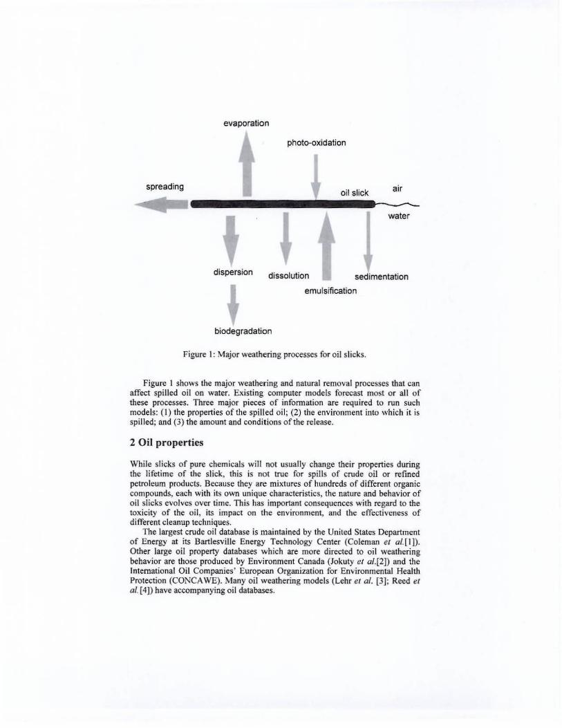
Figure I: Major weathering processes for oil slicks.

Figure I shows the major weathering and natural removal processes that can affect spilled oil on water. Existing computer models forecast mas! or all of these processes. Three major pieces of infonnation are required to run such models: (1) the properties of the spilled oil; (2) the environment into which it is spilled; and (3) the amount and conditions of the release.

2 Oil properties

While slicks of pure chemicals will not usually change their properties during the lifetime of the slick, this is not true for spills of crude oil or refined petroleum products. Bccause they are mixtures of hundreds of differcnt organic compounds, each with its own unique characteristics, the nature and behavior of oi l slicks evolves over time. This has important consequences with ~gard to the toxicity of the oil , its impact on the environment, and the effectiveness of different cleanup techniques.

The largest crude oil database is maintained by the United States Department of Energy at its Bartlesville Energy Technology Center (Coleman ef ai.[I ]). Other large oil property databases which are more directed to oil weathering behavior are those produced by Environment Canada (Jokuty ef a/'[2l) and the International Oil Companics' European Organization for Environmental Health Protection (CONCA WE). Many oil weathering models (Lehr ef al. [3]; Reed et al. [4]) have accompanying oil databases.

2.1 Density

One piece of infonnation included in virtually all the oil databases is the API gravity. This is a scale developed by the American Petroleum Institute and is inversely proportional to the specific gravity of the oil at IS.6°C. Freshwater has an API of 10. Most crude oils and refined products have a higher API (smaller density) than 10 and hence wi ll float in freshwater. However, some heavier refined products and synthetic fuels have a lower API. '!be US Coast Guard groups oils and oil products by the ir densities, referring to these heavier oils (API <10) as Group Vails. Group Vails, if spilled, will usually sink, presenting different cleanup challenges and weathering behavior than floating slicks. Few models exist for sinking oil. Consequently, this paper will concentrate on buoyant oils.

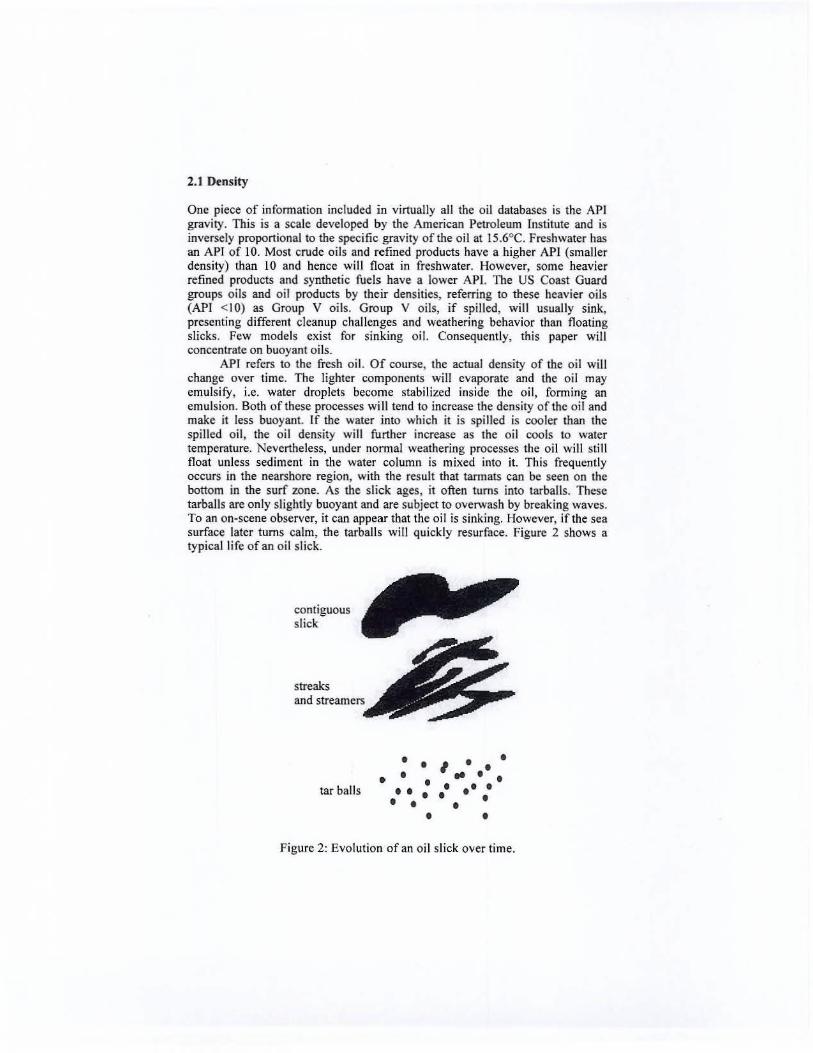
API refers to the fresh oil . Of course, the actual density of the oil will change over time. The lighter components will evaporate and the oil may emulsify, i.e. water droplets become stabilized inside the oil, fanni ng an emulsion. Both of these processes wi ll lend to increase the density of the oil and make it less buoyant. If the water into which it is spilled is cooler than the spi lled oil, the oil density will further increase as the oil cools to water temperature. Nevertheless, under nonnal weathering processes the oil will sti ll fl oat un less sediment in the water column is mixed into it. This freq uently occurs in the nearshore region, with the result that tannats can be seen on the bottom in the surf zone. As the slick ages, it often turns into tarballs. These tarballs arc only slightly buoyant and are subject to overwash by breaking waves. To an on-scene observer, it can appear that the oil is sinking. However, if the sea surface later turns calm, the tarballs will qu ickly resurface. Figure 2 shows a Iypical life of an oil slick.

contiguous slick

streaks

tar balls • • • • • I •• .. .. •• • • ••• •• • • • • • •

Figure 2: Evolution of an oil slick over time.

Most weathering models use the approach of Mackay el al. [5), modified to account for emulsion fonnation (Buchanan and Hurford [61), to forecast the change in oil density,

Here, Cl and Cl are empirically fitted constants that will vary somewhat for

different oils. Reasonable values are 0 .008 X-I and 0.18 respectively.

2.2 Pou r point

Another field in many oil property databases is the pour point o f the oi l. This is defined as the lowest temperature at which an oil will flow under specified cond itions. Pour point is a difficult quantity to quantify and measurements of pour point vary widely. For example, Environment Canada (Jokuty el al. [2]) reports Khafj i crude oil as having a pour point of either -35"C or -48"C. depending upon the reference. While vagucly equivalent to melting point for pure substances, the pour point for oi l, unlike the melting point of a pure chemical, will increase as the oil wcathers. The most commonly used fonnu la to describe this change is an algorithm proposed by Mackay et al.171.

pp= Pp,,(1 + c,j"., ) (2)

Here, Cs is an empirically determined constant. Mackay et al. [7) used the value 0.35 for Prudhoe Bay crude. Others (Daling [8)) use an exponential curve fit instead of the linear relationship assumed in eqn (2). Rasmussen el al. [9] include a linear correction tenn in water content to account fo r the pour point of emulsions as well as pure oils.

2.3 Viscosity

Somewhat related to pour point is the viscosity of the oi l, which is a measure of its resis tance to flow. Roofing tar, for example, is much more viscous than kerosene. There are actually two closely related physical properties that bear the name viscosity: the kinematic viscosity which has units of length squared divided by time, and the dynamic viscosity which is the kinematic viscosity multiplied by the density.The respective SI units are the stoke and poise. These are large units with regard to most flu ids, so the more common centistoke (cSt) and centipoise (cP) are used. The dynamic viscosity and kinematic viscosity of water at 20"C have values close to unity when expressed, respectively, in centipoise and centistokes. Because the density of most o ils differs by less than 30% from water, their viscosity numbers for dynamic and kinematic viscosity are of the same order of magnitude when reponed using these units. Unfortunately, other, less standard units are often selected . For example, one common system of units for kinematic viscosity is SayboJt Universal Seconds (SUS).

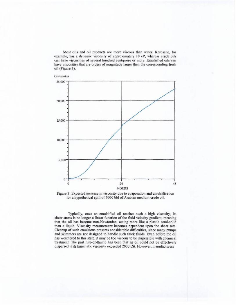
Most oils and oil products are more viscous than water. Kerosene, for example, has a dynamic viscosity of approx imately 10 cP, whercas crude oi ls can have viscosities of several hundred centipoise or more. Emulsified oils ean have viscosities that are orders of magnitude larger then the corresponding fresh oil (Figure 3).

Ccntistokes

25.000

20.000

15,000

'.000 /

/

10,000

o o

V

/

24

HOURS

/ /

48

Figure 3: Expected increase in viscosity due to evaporation and emulsification for a hypothetical spi ll of7000 bbl of Arabian medium crude oil.

Typically, once an emulsified oil reaches such a high viscosity, its shear stress is no longer a linear function of the fl uid ve\ociry gradient, meaning that the oil has become non-Newtonian, acting more like a plastic semi-solid than a liquid. Viscosiry measurement becomes dependent upon the shear ratc. Cleanup of such emulsions presents considerable difficulties, si nce many pumps and skimmers are not designed to handle such thick fluids. Even before the oil has weathered to this state, it may be 100 viscous to be dispersible with chemical treatment. The past rule-of-thumb has been that an oil could not be effectively dispersed if its kinematic viscosity exceeded 2000 cSt. However, manufacturers

now claim that the new class of dispersants can handle oils several times thi s viscosity.

Viscosity is a strong function of temperature. Therefore, it is necessary when usi ng a historical value for an oi l' s viscosity to know the reference temperature at which the viscosity was measured. A commonly used laboratory reference temperature is lOO°F, which is not a oommon temperature fo und at oil spills. Maekay el af. [5] recommend an exponential fonn for the temperature correction function,

v ~v ,"p[e (.!. __ I ll. o ,of ",. r T - (3)

Payne et a/. [10] suggest 9000 K-\ for Cor but the author (NOAA [II]) proposes

a smaller value of5000 K-l , based on laboratory data. As oil evaporates, the relative concentrations of the various components

change . A oommon rule (Perry [12]) is that the visoosity of a nonpolar mixture can be derived from the viscosities of its components, but this is difficult to implement for crude oils because of the large number of oomponents. As an alternative, Buchanan and Hurford [6J suggest that it is necessary only to track one of these components, the asphaltene oontent,

n oc f. ... (4)

However, most modelers prefer to est imate the change in viscosity based on the fract ion of the sl ick that has evaporated. For example, Mackay et af. [13] util ize the fraction evaporated for their oorrelation of weathered oil viscosity with fresh oil viscosity,

(5)

There is no agreement on the method to detenninc c"" Mackay et al. {lJ] say that the tenn depends upon the type of oil. For three different oils that they tested, the numbers ranged from 1.6 to 10.5. Howlett [14] uses I for light fuel s and 10 for heavy fuel oils. NOAA [II] uses a fractional power law fit based on the statistics generated from their oil properties library, with the initial viscosity as the independent variable. Alternatively, they use laboratory results for a particular oil that has been artificially weathered to curve fit eqn (5).

As mentioned earlier, the emulsifying process increases visoosity significantly. Almost all weathering models use the Mooney equation (Schramm (1 5]) 10 forecas t this increase of viscosity with the increase in water fraction Y of the emulsifi ed oi l,

v ~v<xJ~) . 'l - c, .• Y (6)

The choice of2.5 for C" l and 0.65 for C,,2 by Mackay et al. [1 3] is adopted

by most models, although some try to fit them based on laboratory data for the oil of concern. In the latter case, the values for C"l range between 0 and 5. Cy l

ranges between -0.9 and 0.9 (Aamo [16]) or can be estimated, based on average and minimum water droplet size (NOAA [17J).

2.4 Surface tension

Some spreading and dispersion algorithms require knowledge of an oil' s surface tension. Surface tension is the force of attraction between the surface molecules of a liquid. Chemicals which reduce surface tension can be used to facilitate dispersion. Laboratory data exist for the interfacial surface tension between oil and water and oil and air. Mackay el a/. [ 13J proposed the following formu las to describe ehange in surface tension as the oi l weathers:

(7)

S1~ =STN> .(I+ In .. ) . (8)

Rasmussen [18J has recommended that surface tension changes be tracked by a linear superposition of the surface tensions of the pseudo-component relative fract ions (see section 2.5).

2.S Pseudo-components

Petroleum hydrocarbons are grouped into four major categories. Alkanes, al so caJted paraffins, are characterized by single-bonded, branched, or unbranched chains of carbon atoms with attached hydrogen atoms. Alkenes are similar to alkanes, but will have at least one double bond. Aromatics are organics having a benzene ring (or rings) as part of their chemical structures. Naphthenes also form rings, but have single carbon bonds. A small percentage of the oil may consist of non-hydrocarbon compounds Ihat may contain oxygen, nitrogen, sulfur and various trace metals. These constituents, which include such compounds as asphaltenes, can have a significant effect on the way the oil weathers.

Oil components are also commonly grouped on the basis of the boi ling point of the hydrocarbon constituent. Hydrocarbons with similar molecular weights typically have similar boiling points (Jones [l9J). Because much of the information on crude oils is collected for refining purposes, distillation data exist for many oils. Typically, these are given in tabular form, where the oil is broken down into fractions. each fraction reprcsenling a range of boiling point cuts. Oil-spill modelers often take advantage of this information to simulate the very complex hydrocarbon mixture of a crude oil or oil product with a simpler fictitious oil made up of pseudo-components (Payne el al. [lOn, where each component corresponds to one of the distillation fractions. The boiling point of each pseudo-component is the average temperature between consecutive cuts. Other properties of these fictitious components can be approximated as well. The molar volume and molecular weight can be correlated to the boiling point by treating the component as if it were a mixture of alkanes (Jones [20]),

v ...... = c...1 + C,.o,r. + C_,T;,' MW==~I+ C~, r;, + C_, 1~' .

(9) (1 0)

The individual properties of the pseudo-components can also be reassembled to estimate global properties of the orig inal oil. For example, for some evaporation models il is necessary to estimate the ini tial oil boiling point. This ean be done by numerically solving the following equation, using the pseudo-component boiling points and their relative mole fractions:

(11)

Here, the subscript) refers to the individual pseudo-component, and the boiling point tenn without the subscript is for the orig inal oil.

2.6 Flash point

An occasionally important temperature for oils is the flash point, which is a measure of the flammability of the oil. Mackay et al. (7] use a linear fit to fract ion evaporated to estimate change of the flash point over time, simi lar to eqn (2) for pour point. More recently, Jones [21] has re-examined the effects of weatheri ng on fl ash point. He has found that the changing composition of the oil as it evaporates changes the flash point. Using the concept of pseudo­components, Jones suggests thai the flash point can be predicted using a correlation established by Butler el aJ. [21] [22] for middle distillates, provided that the pseudo-components contain infonnation about the low-boiling constituents. Noting that the vapor pressure of each component is a function of temperature, the fl ash point is reached when

(12)

Here, the vapor pressure and molecular weight are expressed in MKS units and the sum is over the number of pseudo-components. This corresponds to requiring the sum of the partial pressure o f the oil volati les to be about I % of an atmosphere. As the oil evaporates, the mole fractions of the less volatile components increase while those of the more volatile constituents decrease. In order to preserve the equality, the vapor pressures must be referenced to an increasing flash point temperature.

3 Environmental (actors

The most general environmental factors affecting oil spill weathering are water temperature, sea state, and wind speed. Also importanl, depending upon the circumstance of the spill incident, are solar radiation, air temperature, water density and salinity, ice cover, and sediment loading in the water.

3.1 Wind

Most oil weathering models are based on wind speeds at a 10m reference height above the water surface. Wind data measured at a different elevation must be adj usted 10 this reference height. Th is can be done by using either a logarithmic (Brutsaert [23]) or a power law approximation. A common fonnula (Brutsaert and Yeh [24]) that will provide reasonable answers provided the measured height of the wind is less than 20 m is

(10)' U,. ==V. -; ( 13)

where z refers to the wind measurement height in meters and the subscripts on the wind speed U specifY the height at which the wind speed is referenced. Furthennore, corrections must also be made if the location of the wind measurement is a considerable distance fro m the spill site, or there are intervening topographical obstructions. Stolzenbach et al. [25] have proposed a scheme for interpolating spatial wind measurements and several oil spill models incorporate this capability. However, for most real spill incidents, a spatially constant wind fi eld is usually employed.

3.2 Waves

Sea state is important for estimating spread, dispersion, and emulsification. A skilled on-scene observer can estimate significant wave height and wave period. However, spill forecas ters often have to estimate these tenus from other factors such as wind spced, fetch, and wind duration. Some simple formulas to petform this task have been developed for tile US Army Corps of Engineers (Coastal Engineering Research Center [26]). For the case of fully developed seas, the sign ificant wave height can be computed, using MKS units, as

H, == 0.0248 .V,l (14)

and the period of the peak of the wave spectrum is estimated by

t. = 0.83 · U. (IS)

where the wind-stress vector V, is calculated by the fonnula

V. ==0.71·U~l) . (16)

The case fo r fetch or duration-lim ited winds is sim ilar. although the fonnulas are somewhat more complicated.

The history of past spills indicates that dispersion or emulsification of the slick often depends upon the presence of breaking waves. Typically, waves will start to break when wind speeds exceed 5 to 10 knolS, but estimating the fraction oft he sea surface that is covered with whitecaps is an inexact science at best Wu

{27], Monohan and O'Muircheartaigh [28), Holthuijsen and Herbers [29], and O 'M uircheartaigh and Monohan [30] provide some guidance but their data shows wide scatter. The NOAA [1 1J weathering model uses a cubic polynomial fit

0 5./ ... 5. 1 (17)

which cuts off whitecap generation below 3 mis, acts almost as a linear equation for wind speeds of 8-12 mls and increases whitecap fraction rapidly for high wind speeds.

3.3 Solar radiation

Photo-oxidation of spilled oil depends upon solar radiation. Experiments (Overton [31]; FaIT (32]) indicate that solar radiation may contribute to crusting on the surface of the sl ick and impede other weathering processes. The flux of solar shortwave radiation at the top of the atmosphere is 1367 W/m 2. Approximately 17-20% of it is absorbed by the clear atmosphere, and clouds act to reflect or absorb even more. It is possible to estimate ground-level radiation flux levels based upon time of day, date, latitude, and cloud cover (NOAA [33]).

4 Spill release

Many weathering models assume an instantaneous release of the oil, an unrealistic condition for large spills. Weathering models that are connected to a trajectory model (Appl ied Science Associates [34]) often will allow the user to vary the amount spilled over space and time but typically give little guidance for estimating these terms. There has been surprisingly little research into oil release behavior, although current research anicles (Simccek-Beatty et af. [35]; Rye [36); Yapa and Zheng [37]) indicate that this may be changing.

4.1 Subsurface release

Of particular concern arc releases that are subsurface. Subsurface releases that are low pressure, such as releases from sunken vessels and some ruptured pipelines, typically fonn a • fl ower blossom ' pattern, where the oil spreads out thinner than it would during a surface release of the same amount of oil. Leaks caused by blowouts from offshore wells can produce an init ial surface slick of already emulsified oil.

As drilling has moved into ever deeper waters, a major quest ion remains as to whether a surface slick will appear at all from a release at the ocean floor. A key factor in answering this question will be found in the transition 7.one where the release ceases to be described by a jet of water, oi l and gas, and becomes a cloud of buoyant oil droplets that may, or may not surface, depending upon the droplet size distribution.

Model development of deep-water releases is still an active research area and discussion of the various proposals is outside the scope of this essay. The reader is refelTed to Rye (36) and Yapa and Zheng (37].

4.2 Leaking tankers

Simecek-Beany et 01. [35] have modeled the release ofa holed tanker by treating it as an idealized cylindrical tank. They identify three different leak scenarios.

The most simple is a release of oil from above the water line, where the tank itself is open to the atmosphere. Then, the flow rate is determined strictly by Bernoulli 's equation,

( \8)

If the hole is below the water line , there may be water ingestion as well as outflow of oil . The detennining factor is the equilibrium height, defined as

z - z Z 0:= PM. p ... -ail

., P~ -p .. (\9)

If the equ ilibrium height is above the hole height, only water will fl ow in, fanning a water bottom in the tank. If the equilibrium height is below the hole height, only oil wi ll be released until the equilibrium height reaches the hole height, at which time both water ingestion and oil outflow wi ll occur.

The third leak scenario is the situation where the tank is not open to the atmosphere and a vacuum forms inside the tank, slowing the release of the oil and causing air ingestion to equalize the pressure. Such a situation occurs if the tank's vacuum relief valve is damaged or del iberately closed by the crew to slow the release of the oi l.

Whatever the mechanism that describes the oil release behavior, oil that is released over a time period comparable to the time it takes for the oil to spread over the water will have different area coverage than the same amount of oil that is spilled quickly. This can have consequences for those weathering processes that are strong functions of slick area.

5 Weathering processes

Weathering processes can be divided into three categories. Rapidly occurring processes have immediate consequences for the spill response. Such processes include spreading, evaporation, dispersion, dissolution, and emulsification . Other weathering mechanisms operate more slowly and are important usually in regard to studies of the long-tenn effects of the spill. Examples include photo­oxidation and biodegradation. Finally, there are some processes that arc important only under part icular environmental conditions. Such processes include sedimentation and oil-ice interaction.

5.1 Sp readin g

The rate at which oi l spreads on open water can affect other weathering processes such as dispersion, evaporation and emulsification. The cleanup itself needs accurate information on expected spill size when planning such strategies as

skimming operations or dispersant use. Unfortunately, spreading is an immensely complicated phenomenon involving both the physical properties of the spilled product and the environmental state of the surface water on which it is floating.

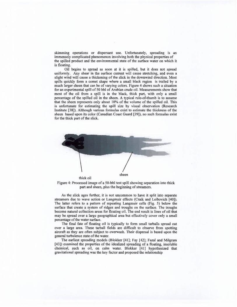
Oil begins to spread as soon at it is spilled, but it does not spread uniform ly. Any shear in the surface current will cause stfCtching, and even a slight wind will cause a thickening of the slick in the downwind direction. Most spills quickly fonn a comet shape where a small black region is trai led by a much larger sheen that can be of varying colors. Figure 4 shows such a situation for an experimental spill of 50 bbl of Arabian crude oil. Measurements show that most of the oil from a spill is in the black, thick part, with only a small percentage of thc spilled oil in the sheen. A typical rule-of-thumb is to assume that the sheen represents only about 10% of the volume of the spilled oil. This is unfortunate for estimating the spi ll size by visual observation (Research Institute [38]). Although various formulas exist to estimate the thickness of the sheen based upon its color (Canadian Coast Guard [39]), no such formulas exist fo r the thick part of the slick. .

sheen thick oil

Figure 4: Processed image ofa 50-bbl test spill showing separation into thick part and sheen, plus the beginning of streamers.

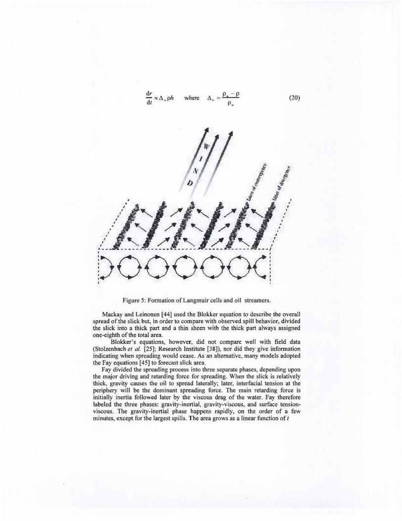
As the slick ages further, it is not uncommon to have it split into separate streamers due to wave action or Langmuir effects (Craik and Leibovich [401). The laner refers 10 a pattern of repeating Langmuir cells (Fig. 5) below the surface that create a system of ridges and troughs on the surface. The troughs become natural collection areas for floating oi l. The end result is lines of oil that may be spread over a large geographical area but effectively covcr only a small percentage ofthe water surface.

The fina l fate of floating oi l is typically to fonn small larbaJls spread out over a large arca. These tarball fields arc difficult to observe from sponing aircraft as they arc often subject to overwash. Their dispersal is based upon the general turbulence state of the water.

The earliest spreading models (Blokker [41 ]; Fay [42); Fazal and Milgram [43]) exam ined the properties of the idealized spreading ofa floati ng, insoluble chemical, such as oil, on calm waler. Siokker [4 1J hypothesized that gravitational spreading was the key factor and proposed the relationship

where .6 = P. - P • p.

(20)

Figure 5: Fonnalion of Langmu ir cells and oil streamers.

Mackay and Leinonen [44J used the Blokkcr equation to describe the overall spread of the slick but, in order to compare with observed spill behavior, divided the slick into a thick part and a thin sheen with the thick part always assigned one-eighth of the total area.

Blokker' s equations, however, did not compare well with field data (Stolzcnbach el al. [25]; Research Institute [381), nor did they give infonnation indicating when spreading would cease. As an alternative, many models adopted the Fay equations [45] 10 forecast slick area.

Fay divided the spreading process into three separale phases, depending upon the major driving and retarding force for spreading. When the slick is relatively thick, gravity causes the oil to spread latera lly; later, interfacial tension at the periphery will be the dominant spreading force . The main retarding force is initially inertia followed later by the viscous drag of the water. Fay therefore labeled the three phases: gravity-i nertial, gravity-v iscous, and surface tension­viscous. The gravity-inertial phase happens rapidly, on the order of a few minutes, except for the largest spills. The area grows as a linear function of t

A = 0.57nJA..gV.( (21)

unti l the time (Dodge et af. [46]) when the relative thickness is small enough that the transition to gravity-viscous spreading occurs . Th is time is calculated by the fonnula

(22)

The area at this transition time is often taken as the initial area for many spread models . It is given by the formula

(23)

The area then continues to grow according to the gravity-viscous term

(24)

unti l it becomes so thin that surface tension becomes the driving force. The area for this phase is described by the algorithm

A = 2.6Jt · where (25)

Other researchers (Waldman ef al. [47]) have derived slightly differeOl values for the empirical coeffic ients used in the above equations, or have other small variations in the form ulas for one of the phases (Buckmaster [48J). Mackay el aJ. [49] have appl ied Mackay's concept of a thick-thin slick combination using the Fay form ulas. Garcia-Martinez et aJ. [50] proposed modifying some of the constants in the Mackay method to account better for the oil and water physical propenies.

Although the Fay fonnulas are theoretically sound, they have perfonned poorly in actual spi lls. In most repo ned cases, they have underestimated spill area (Murray [51]; Conomos [52]; Lehr et af . [5 3}), whereas in at least one case, they significantly overeslimated the area (Ross and Oickins [54]). Also, Jeffery [55] noticed no transition betwecn the d ifferent spreading phases. Lehr et af [56] have pointed out that only the gravity-viscous phase happens in the time frame when spill response is typically occurring.

There have been numerous suggestions on how to improve the Fay spreading fonn ulas. Plutchak and Kolpak [57) claimed that the change in surface tension and density due to weathering needed to be determined to use Fay spreading

optimally. In order to account for wind spreading effects, Lehr et al. [56] proposed altering the shape of the spill from a circle to an ellipse with the long axis being parallel to the wind. Considering only gravity~viscous spreading to be important, they proposed the area to be estimated by (MKS units) . ,

A= 2.27(A. V); .,' +O.04(A.vu')., . (26)

Curiously. the Fay equations do not depend upon the viscosity of the spilled oil, while common sense says that a heavy fuel oil would spread more slowly than a light refined product like gasoline. Ross and Energetex Engineering [58] modified the Fay equation by inserting a correction facto r that is equal to the oil-to-water viscosity ratio raised to the 0.15 power. El-Tahan and Venkatesh [59] introduced the concept of 'velocity gradient' which is inversely related to the oil viscosity and represents vertical shear resistance in the o il slick .

However, it is doubtful that any mere patches to the Fay formulas will allow accurate prediction of slick area over any extended time period because of the neglect of outside environmental factors and details of the initial release. As an alternative, researchers have attempled to model slick spreading as strictly a water turbulence phenomenon with the oil acting as a neutral tracer (Murray [51]). When a neulrally buoyant dye is dropped onto the ocean surface, the dye begins to disperse due 10 water turbulence. The area of sea surface covered by the dye will grow as a function of time and a suitably defined eddy diffusion coefficient,

(27)

Presuming that this same phenomena affects the dispersion of positively buoyant spilled oi l, Ahlstrom (60] has recommended simu lating this process by dividi ng the oil inlo a suitable number of separate elements, often referred to as Lagrangian elements, and then randomly displacing these elements over time using a properly chosen eddy diffusion coefficient. Elliot et al. [61] conclude that such a process is non-Fickian. and that a time-dependent diffusion parameter better represents empirical results. Their diffusion parameter is (MKS units)

D ... , = 0.033!" " . (28)

It is possible to incorporate Fay spreading with diffusive spreading by treating the former as a pseudo-diffusion process and matching rwice the standard deviation of the distribution of oil element locations with the radius of the oil slick as predicted by the standard Fay formula. This yields a Fay pseudo­diffusion coefficient of

JA gV')l I D ... =0.1\ 7 Ji (29)

Another approach is to allow the individual elements to spread according to Fay spreading rules, treating these elements as ' minispills '(ASA [34]). The minispills are then dispersed and moved by water turbulence and other forces. Care must be taken not to bias the results by the number of elements seleeted and to handle interaction between the elements properly.

Evell including water turbulence. Fay spreading is still incomplete, however (Lehr [62]). Probably the most important cause of long term oil spreading is wind stress on the slick and surface water. Unfortunately, this is a complicated phenomenon that is ollly partly understood. Observations at past spills have resulted in a rule-of-thumb that the o il slick moves at approximately 3% of the wind speed measured at 10 m above the water surface. Roughly two-thirds of this movement represents Stokes drift of the surface waves. The remaining one­third represents the movement of the slick along the water surface. Also, oil is driven into the water column by breaking waves and broken into droplets of different size (Dclvigne and Sweeney [63]). The larger droplets quickly resurface while the smaller droplets remain subsurface for longer time periods and trail the moving main slick. Elliot et a/.(6 1) hypothesize that this is the cause for the 'comer shape of many slicks where a thicker pan of the oi l at the upwind pan is encompassed in a larger sheen which trails out behind the thick part. The smallest droplets never resurface and are thus permanently removed from the surface slick. Proper modeling of such phenomena requires a numerical simulation of the lIear surface water flow (lborpe [64]). However, an often adequate alternative is to use a boundary layer approach (Elliot [65]) where the horizontal current velocity follows a logarithmic profilc and the vertical velocity is calcu lated by using a suitably modified fonn (Kolluru et al. [66]) of Stokes L,w

w _ (drop) ' g6. ~- 18v. (30)

As mentioned earlier, oil slicks often break inlO wind rows due to the effects of Langmuir circulation. It is generally believed that Langmuir circulation is produced by the illleraction of surface currents and Stokes drift due to waves (Csanady [67]). Thorpe [68] and Farmer and Li [69] have sketched an outline of how to include Langmuir effects in weathering models but, at present, none of the widely used models includes this feature.

There are other factors which can easily affect the area of a slick. Mosl spreading algorithms assume instantaneous release of the spilled o il and open water conditions. However, real spill incidents may be causcd by leaks which continue al a varying rate for hours o r days and occur near a shoreline or other impediments to spreading. Changing currents from tides or other forces will aher spreading patterns. Human interference through skimming and booming will modify slick area. The importance of any of these factors will depend on the spill incident.

Eventually, all slicks stop spreading. They may even shrink due to wave stress. They also break into increasingly smaller patches. The Fay fonnulas theoretically allow a mechanism for spread ing to stop (Mattson and Grose [70]). If the net radial surface tcnsion is negative, the oil should stop surface tension­viscosity spreading and, instead, contract into a lens with its thickness

controlled by gravity. In practice, a lternative stopping mechanisms based on spill volume or thickness are used instead by most models. Fay (45) himself recommended that the final area be estimated from the initial volume,

! A,'" V' (31)

Dodgc el a/.[46J state that the slick effectively stops spreading whcn the thick pan of the slick reaches a thickness of 0.1 mm. Many models use this value for crude oils and a smaller number for light refined products (Reed [71). There is little accurate empirical information on final spill thickness from real spi lls because techniques to perfonn the measurements are crude and unreliable, and are seldom perfonned in any casc.

Consideration must be given to the numerical techniques used in simulating spreading. As spreading algorithms incorporate more features, an analytic solution becomes increasingly impractical. A numerical solution, using the Lagrangian element method, is the normal choice for many models. While the ' minispill ' approach mentioned earlier is computationally attractive, it has some inherent drawbacks. Such an approach neglects thc fact that the forces acting on the slick are interconnected and non- linear in oil volume. More imponantly, it ignores the fact that all the above-described processes are acting simultaneously on all the spilled o il. Separation of the slick into distinct patches is a naturally occurring mechanism and should, ideally, be the end result of the modc1ing process rather than pre-defined as to shape and number by the modeler. An alternative technique is leave the Lagrangian elements as distinct points that are equally subject to all the physical forces described. Oa[t[72] describes a method for translating a set of distinct points into a continuous distribution for area calculations by utilizing Thiessen polygons.

5.2 Evaporation

Probably no area of oil weathering has been more studied and tested than evaporation. It is therefore surprising that there is still considerable controversy on the exact mechanism controlling evaporation rale. It is, however, not at all surprising that the reason for any disagreement can be traced 10 the fact that the oil is a mixture and not a pure chemical.

Certain points are agreed upon by experts in the field. It is recognized that, for most spills. evaporation is the major mechanism for mass removal from the surface slick. This includes both natural processes and cleanup attempts. It is quite possible to lose half of a light crude spill just due 10 evaporation. Small, light refined product spills will typically disappear in less than a day due to evaporation unless high sea states drive the oi l into the water column.

Also, evaporation changes the chem ical mixture of the slick as the lighter components evaporate more quickly than the heavier hydrocarbons. The structure of thc molecule is of some importance. Aromatics, for example, lag behind paraffins. However, the major factor is molecular weight. The vapor pressures of hydrocarbons with a carbon number of 10 or above are orders of magnitude smaller than the vapor pressures of hydrocarbons with carbon number of 6 or below. If the only infonnation needed for cleanup is, say, how much oil will

reach a beach after a week at sea, it may not be necessary to calculate a time­dependent evaporation rate for the slick. Instead, it may be suffi cient to simply determine which fractions will, or will not, evaporate. Smith and Macintyre [73] found that very linle of any distillation cut with a boiling point above 270°C will evaporate. This corresponds to a cutoff for non-evaporation of all hydrocarbons with 15 carbon atoms or more.

Most spill weathering models base their evaporation algorithms on the assumption that the o il slick can be treated as a ven ically homogeneous mixture . This 'well-mixed ' assumption allows, with suitable modification, the use of evaporation estimation techniques developed for homogeneous liqu ids (Brutsaen (23]). The driving factor for evaporation will be the effective vapor pressure of the oil and the limiting factor will be the ability of the wind to remove the oil vapor from the surface boundary layer.

Given the well-mixed assumption, there are two general approaches to calculating evaporation rates. The fi rst approach is the pseudo-component method (Payne el al. [10]; Jones [20)), where, as mentioned earlier, the oil is postulated to consist of a limited number of components, with each component corresponding to one of the cuts from the distillation data for the oil of concern . Each component is characterized by a mole fraction and a vapor pressure. The evaporative flux of each component is assumed to be a function of the vapor pressure of the liquid phase of the component

(32)

where the j subscript refers to the individual pseudo-component. Assuming Raoult 's Law for an ideal mixture, the total evaporation rate is given by the sum of the individual rates. Note that whi Ie the overall evaporation rate for the slick decreases with time, it is possible for the evaporative flux of a particu lar component to increase if the mole fraction of that component increases.

Different researchers have different expressions for the mass transfer coefficient K . Mackay and Matsugu (74] suggest a mass transfer coefficient related to the Schmidt number. which is defined as the ratio of the kinematic viscosity to the molecular diffusivity.

.J K, _(So,)' (33)

Since there arc different Schmidt numbers for each of the pseudo-components, there would theoretically be different mass transfer coefficients for each component as weI!. In practice, however, an average value, related to 7/9 of the wind speed, is usually used (Mackay and Leinonen [44]). Typical ranges for K are between a 0.5 and 2 cm/s. Williams el al. (75] proposed an exponential function of the wind speed for the lighter hydrocarbons and a constant value for the heavier ones. Others use a mass transfer coefficient thaI is linear in wind speed.

The oil temperature in the denominator of eqn (32) is usually set to the ambient water temperature, although some models have used the air temperature instead. Because of oil ' s insulating capabilities, and the effects of solar radiation

on the dark slick, oil sl icks which are contained and thick may, in fact, have a surface temperature that is much warmer than the surrounding water or air temperature (Mackay and Matsugu [74); lones el aJ. [76]).

In reality, the mixture of hydrocarbons that makes up an oil slick is not an ideal mixture and Raoult's Law is not striclly true. There is the heat of solution caused by the mixing, in addi tion to the heat of vaporization, that must be ovcrcome for evaporation to occur. One way to correct for this is to reduce the pseudo--component vapor pressure by multiplying it by an activity coefficient which is slightly less than one (Stolzenbach et al. [25]).

Rather than deal with the complexities of the pseudo--component model, Mackay et al.17J suggestcd treating the slick as if it were a single-component fluid with changing properties due to weathering. They introduced the idea of a dimensionless variable e called evaporative exposure,

KAt 0 = - v. (34)

which was proportional to time but had a linear relat ionship to fract ion evaporated

(35)

II is important to note that the above equation uses the liquid-phase boiling point temperature rather than the more common vapor·phase temperature. It also assumes that the liquid distillation curve can be adequately characterized by a straight line, which may not be correct in some cases.

The mass transfer constant in this model, often referred to as the Stiver­Mackay model, has a sim ilar form to the one used for the pseudo·component mode\. Stiver and Mackay [77] recommend

K = o.o02u"" . (36)

The dimensionless constants a and b in eqn (35) arc empirically fit , Mackay ef af. [7] suggest

a = 6.3 b=10.3 , (37)

whereas Bobra [7S] and Belore and Buist [79] determine a and b values for specific oils through laboratory measurements and a curve-fitting process. Unfortunately, a and b are not independent, and small experimental and curve fitting errors can generate widely varying values for them. Also, Overstreet er al. [SO] showed that model results were, in some cases, highly sensitive to r.. , which itsclfmust be estimated through laboratory measurements .

Jones [20} found that the Stiver-Mackay model generally predicted larger evaporation amounts than his version of a psuedo-component model. Recently, Reed el 01. [SI] have questioned the linearity assumption implicit in the exponent in eqn (35) for some oils.

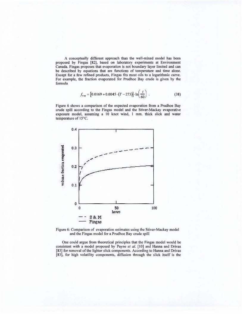
A conceptually different approach than the well-mixed model has been proposed by Fingas [82J, based on laboratory experiments at Environment Canada. Fingas proposes that evaporation is not boundary layer limited and can be described by equations that are functions of temperature and time alone. Except for a few refined products, Fingas fi ts most oils to a logarithmic curve. For example, the fraction evaporated for Prudhoe Bay crude is given by the fonnu la

I~ = [0.0169 +0.0045· (1' - 273)J.ln(6~l (38)

Figure 6 shows a comparison of the expected evaporation from a Prudhoe Bay crude spill according to the Fingas model and the Stiver-Mackay evaporative exposure model, assuming a 10 knot wind, I mm. thick slick and water temperature of 15°C.

1 ~ • • .S

] j g

0.4 ,------,-, -------,

0.3 I-

0.2 I -­,---,

i~ 0.1 f-

-- _.--_ .. ---

-

O~--------~I--------~ o

S&M Ping ..

SO ho""

100

Figure 6: Comparison of evaporation estimates using the Stiver-Mackay model and the Fingas model for a Prudhoe Bay crude spill

One could argue from theoretical principles that the Fingas model would be consistent with a model proposed by Payne et al. [10] and Hanna and Drivas (83] for removal of the lighter slick components. According to Hanna and Drivas [83], for high volatility componenls, diffusion through the sl ick itself is the

mechanism limiting their evaporation rate. The presumption is that, shortly after the spill happens, the volatiles close to the surface are preferentially removed, leaving behind the larger molecules with lower vapor pressure. The volatile compounds deeper into the slick then migrate to the surface, creating a concentration gradient within the slick. This diffusive process, and not boundary-layer effects, is the limiting factor controlling evaporation of these lighter molecules. Hanna and Drivas [83] develop an inequality to detennine whether a component,j, is diffusion limited. In slightly modified form, it is

(39)

Provided this time-dependent inequality holds, the process is diffusion-limited. If so, the governing equation is the one-dimensional diffusion equation for the concentration of the particular volatile component being modeled

(40)

A major difficulty is to estimate the appropriate value for the diffusivity D .... . Hanna and Drivas [83] use a correlation for organic/organic liquid diffusivity from Perry [12]

(41 )

Typically, the volatile component selected is benzene since it is the lightest of the aromatic compounds and is a known human carcinogen. The benzene content of crude oil averages about 0.2% and is higher for certain refined products. Holliday and Park [84] review some of the work on modeling benzene and other oil vapors.

A third possibility for evaporation was proposed by Payne el al. [to] and by Lehr [85]. Both suggest that, under cenain conditions, while most of the slick is well-mixed, a thin crust may form and impede evaporation. Photo-oxidation could playa role in the fonnation of such a crust.

5.3 Dissolution

The old saying that oil and water do not mix is scientifically accurate when it relates to molecular dissolution of oil into the surrounding water. Dissolution is unimportant for estimating the mass balance of the slick. Removal by this process is orders of magnitude smaller than evaporation. Furthennore, components that do dissolve may later evaporate from the water surface. Unfortunately, the more soluble hydrocarbons are likely to be the more toxic, so that even small concentrations may have adverse biological consequences.

Few models exist for dissolution. Mackay and Shiu [86] have measured the aqueous solubility of fresh and weathered crude oil. Payne el al. [101 and Mackay and Leinonen [44J have constructed pseudo-component models similar to the ones used for evaporation . For example, Mackay and Leinonen [44J calculate the dissolution flux for pseudo-componentj according to the fonnula

(42)

The key factor in properly estimating dissolution is estimating the surface area of any dispersed oil, since dissolution is apt to be much faster from the dispersed droplets than from the surface slick. Based on mass transfer rate measurements, Mackay and Leinonen [44J suggest a Sherwood number (the ratio of the droplet diameter times the mass transfer constant to the diffusivity in the water) of about 2. They conclude that, for droplets less than 0.1 mm in diameter, dissolution is very rapid for any component that will dissolve at all. Any remaining material in the droplet will consist of relatively insoluble hydrocarbons, i.e. hydrocarbons with a carbon number greater than about 10.

5.4 Dispersion

While oil may not dissolve in water to any great extent, it can certainly disperse as a cloud of droplets when subject to turbulent wave energy . These droplets will be in various sizes, and will be subject to the conflicting forces of buoyancy and turbulence. For the smallest oi l droplets, as for the smallest dust particles in the air, turbulence will win the battle and the droplet will not refloat to rejoin the slick. For slicks of low viscosity oil under high sea state conditions, dispersion becomes the dominant mechanism for removing spilled oi l and can easily displace 90% or more of the surface slick.

The early models (Blaikely el al.[87]) of dispersion simply assumed a constant dispersion rate as percentage of the oil slick per day, based on the sea state . These numbers tended to be quite large, from 10 to 60% per day. This was an overestimate for large, weathered oil slicks.

Mackay et af. [49] also constructed a fonnu la that computed a fractional rate of removal of the slick by dispersion. Rather than using a simple look-up table based on sea state, their model was a product of two factors. The first factor calculated the fraction of the sea surface subject to dispersion and the second factor estimated the fraction that would not rejoin the slick, staying pennanentiy dispersed instead.

About the same time, Aravamudan et al.[88J, developed a somewhat inappropriately named simpli fied model to calculate dispersion. While too complex to gain wide acceptance, it laid the foundation for other models that followed. It not only calculated the rale of dispersed oil droplet fonnation based o.n the fraction of breaking waves, but also predicted the distribution in droplet sIzes.

Most weathering programs now use some version of the dispersion model developed by Delvigne and Sweeney [63]. For this model, the entrainment of oil is estimated as

(43)

where the dissipation of wave energy per unit area is given by

2\ = O.OOI7·gp .. H: (44)

and the fraction of breaking waves per wave period j"", is estimated to be

(45)

f .. is obtained (to within a constant) by integrating the product of the droplet

volume and the frequency distribution of droplets over the volume of oil. In practice, thc integration is performed between the minimum droplet size and maximum droplet size, determined from cxperimenlal data. This yields

(46)

where a maximum droplet size 6 max is usually set equal to the maximum droplet size that would not be expected to refloat, based on Stokes Law or experimental observation. Typically. this is about 50 to 70 microns. Larger droplets than this will refloat faster than the surface slick can traverse the area covered by the dispersed oil and hence will rejoin the surface slick. Drops 70 microns or smaller arc effectively held in suspension as shown by examining the steady-state tail of the droplet diameter versus refloat time curve as measured by Delvigne et al. [89). Reed et al. [81J have objected to using a fi xed droplet size as a criterion for refloating, pointing out that the lim it for pennanent dispersion should be related to droplet rise velocity and sea state. A commonly used, although not necessarily correct, minimum droplet size is 5 microns.

N(!J), the number of oil droplets per unit volume of water per unit droplet diameter, is a function of droplet size

_i N{b)ocb ) (47)

The experimentally determined parameter c""" is highly sensitive to the viscosity

of the oil (Figure 7). As the slick becomes more viscous, the energy required to tear it into small droplets increases and its dispersibility decreases. Laboratory model studies (Delvigne {90D showed that droplet entrainment is difficult when the slick's kinematic viscosity exceeds 3000 cSt.

The dispersed oil droplets are presumed to be initially distributed unifonnly throughout the water column to a depth of 1.5 wave heights. The larger droplets retum 10 the sl ick while the smaller droplets diffuse through the water column. Mackay et al. [91] have proposed a constant vertical diffusion coefficient of over 100 square centimeters per second for use in estimating this dispersion. Others have suggested using a diffusion coefficient scaled to the

existing wind speed and current in the area of the slick. Farmer and Li [69] argue that the effects of Langmuir circu lation must be taken into account when estimating subsurface oil concentration. While wave energy dominates the mixing process in the first few meters, Langmuir cells are more important for greater depths. Therefore, diffusion coefficients may have to be properly determined based upon the appropriate depth scale.

2000,----------------------------,

1500

1000

500

centistokes

Figure 7: Plot of empirical dispersion constant versus viscosity.

5.5 SWimentation

Sedimentation is defined as adhesion of oil to solid particles in the water column.The significance of sedimentation as an important removal process depends critically on the sediment load of thc surrounding water. For muddy rivers, where the sediment load can bemore than 0.5 kglm3, the removal by sedimentation is considerable and exceeds the loss due to normal dispersion. For open ocean conditions, where sediment load is less than 1% of this amount, removal by sedimentation is tr ivial.

The actual physical process of sedimentation is quite complicated and has been only fragmentarily researched. Studies by Poirier and Thiel [92] and by Hartung and Klinger [93] indicated that the process is affected by type and size of the suspended material, salin ity of the water, and sulfur content of the oil.

Others have suggested that oil droplet size, wh ich is directly related to oil viscosity and wave energy, plays a significant role. One fonnula proposed by Science Applications International (Payne et 01.[94]) computes the mass of oil lost per unit water volume per unit time as

q ... :: k./fC ... C .... (48)

The slicking parameter k. depends on the type and size of the particle. Typical

values would be on the order of 100 cm3/kg of material. The energy dissipation rateE can be estimated by the breaking wave energy calculations described previously. In fact, the assumptions that are included in the Oelvigne dispersion model can be combined with this model to yield a fonn ula for the total sedimentation rate per unit area of the slick. This involves integrating over the water depth that the breaking waves drive the oil droplets,

l .l lI.

Q. : Jq~ ", (49) •

The combined oil-sediment particle will typically have a different buoyancy than either alone. Usually, the buoyancy will be negative. and turbulence will be required to keep the oil-sediment particle from settling to the bottom.

5.6 Emulsification

Emulsifi cation is the reverse of dispersion. Rather than oil droplets dispersing into the water column, water is entrained in the oil. This causes significant changes in the volume, densi ty, and, especially, viscosity of the slick. It is not uncommon for the viscosity of an emulsified oil to be two or three orders of magnitude larger than the viscosity of the fresh oi l. This has important implications for cleanup policy, as many common cleanup tools may be rendered ineffective when the oil becomes too viscous.

Not all oils will emulsify and some oils will emulsify only after they have weathered to a certain extent. Caneveri and Fiocco [95] concluded that trace metal content may playa factor in the emulsification of fresh crude oils. They assert that oils with vanadium and nickel content above 15 ppm readily emulsify whereas those with less do not. However, for most oi ls, it appears that wax and, most importantly, asphaltene content play the dominant role in detennining whether emulsification will occur. Waxes and asphaltenes may be considered as solutes in a solvent consisting of the lighter hydrocarbon components of the oil. As the oil weathers and loses the light ends, these large molecules may precipitate out, fonn ing crystals that stabilize small water droplets in the oi l (Bridie el al.[96J). Resin level may playa role as well, since resins help to maintain asphaltencs in solution (Speight [97]) but also can act alone as effective emulsifiers (80bra [98]). A common, but not necessarily reliable, rule-of-thumb, is that crude oil will emulsifY when the wax and asphaltene content reach 5% of the mass of the oil.

Light refined products generally will not emulsify since they do not contain

the right hydrocarbon components to stabilize the water droplets. In rare cases, old diesel spills appear to emulsify, perhaps due to the creation of emulsifYing molecules by photo-oxidation. Bunker fuels may fonn weak emulsions with relatively low water content.

Fi ngas and Fieldhouse (99) have reccntly divided oils into three categorics, bascd on their abil ity to fonn stable em ulsions. They classify stable emulsions as those that retain their water content over time and show very large increases in viscosity. Stable emulsions have suffici ent asphaltene content, typical1y greater than 5%, to stabilize the water droplets in the oil. Mesostable emulsions have insufficient asphaJtenes to make them completely stable. They will lose some of their water content if left undisturbed and will show viscosity increases an order of magnitude less than stable emul sions. The third category is unstable emulsions, which will lose practically all their water content if left at rest.

As mentioned earlier, the onset of emulsification is important for cleanup decisions and it is therefore usefu l fo r a weathering model to have the capabi lity to forecast this event. Unfortunately, the best way to do this is to use observational data from actual spills. Since this is not avai lable except for a handful of oils, results from small test slicks or laboratory data from artificially weathered oil must be used instead (Oaling et al. (1 001). Sometimes, estimates ean be made on new oils by comparing them with tested oils of similar composition.

Once an oi l begins to emulsifY, the process typically proceeds at a rapid rate. Most models use the simple fi rst-order rale law proposed by Mackay et aJ. [49]

dY ,( y ) - = k U 1- - . dl '" y_,

(50)

A typical value lor k_ is I to 2 ms/m2 of slick. Daling and Brandvik [101] concluded that the specific value depends upon the type of oil and its state of weathering. However, the range of values appears to be small for most crudes. Also, the transition time from non-emulsified oil to emulsified oi l is usually smaller than the expected error in estimating the onset of emulsion fonnation. Consider the example of an oil with a water uptake parameter of 1.5 ms/m 2 and a ma.ximum water content fraction of 0.75 exposed to 10 m/s wind. The time for the oil to reach 95% of complete emulsification according to eqn (50) is about 4. It is very unlikely that the onset of emulsifi cation could be detennined to this accuracy in a real spill situation .

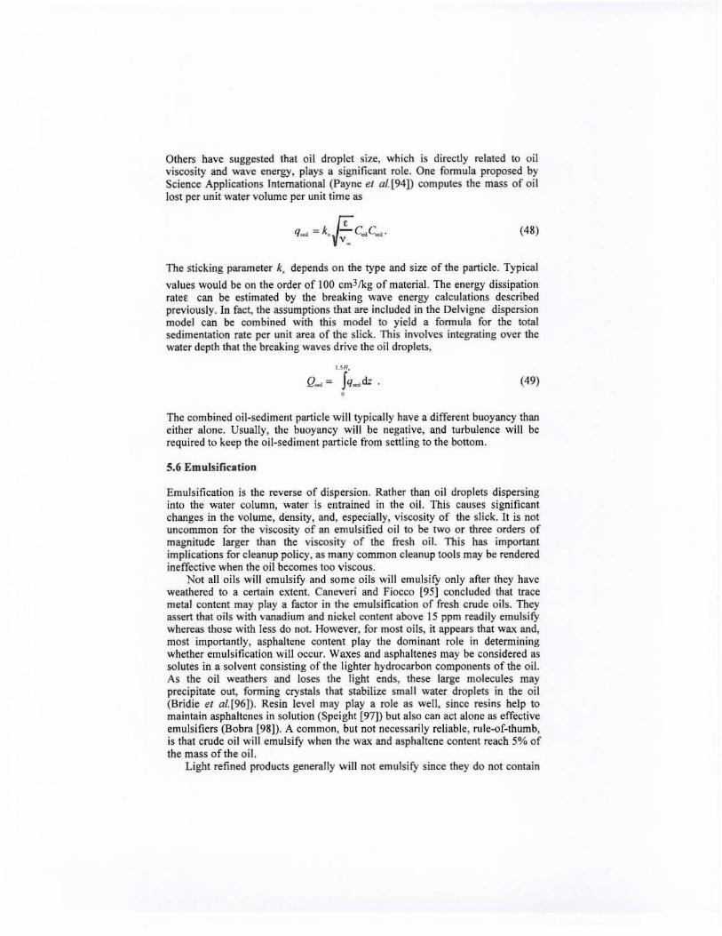
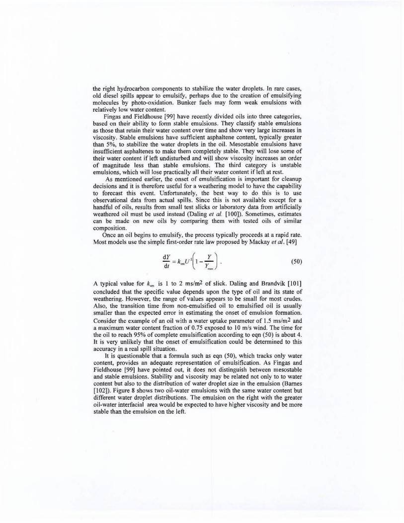
It is questionable that a formula such as eqn (50), which tracks only water content, provides an adequate representation of emulsification. As Fingas and Fieldhouse [99] have pointed out, it does not distinguish betwt:cn mesostable and stable emulsions. Stability and viscosity may be related not only to to water content but also to thc distribution of water droplet size in the emulsion (Barnes [1021). Figure 8 shows two oil-water emulsions with the same water content but different water droplet distributions. The emulsion on the right with the greater o il-water interfacial area would be expected to have higher viscosity and be more stable than the emulsion on the left.

oil

Figure 8: Two different possible water droplet distributions in emulsified oil

Eley el ai, [103] have suggested using a first-order equation in interfacial area

dS = k( I -~) dl ' S,..,

(lI)

where the intcrfacial parametcr k, is sensitive 10 wave energy (NOAA [17])

k, C(; U' . (52)

6 Other processes

The two long term mechanisms for the breakdown of hydrocarbons in the environment are photo-oxidation and biodegradation. For spills in a cold environment, oil-ice interactions may be important.

6.1 Photo-oxidation

The combination of hydrocarbons with oxygen is called oxidation. The newly fonn ed oxidized compounds may affect the oil slick by increasing dissolution, dispersion or emul sification. While trace metals in the oil may influence the oxidation process, ultraviolet light sig nificantly increases oxidation. Virtually all of the molecules that evaporate from the slick undergo photochemical oxidation in hours or days (Altshuler and Bufalini [104); Heicklen [105]). Also, beached oil will show the effects of exposure to sunlight. Even floating oi l can show chemical changes due to this process. Overton [31} exposed IXTOC I crude oil to sunlight and discovered the formation of tarry flakes, showing the involvement of photolysis. Observers at the Mega Borg spill in the Gulf of Mexico noticed the formation of crus Is on floating tarmats and tar balls, with the

hypothesis that this was due to photo-oxidation. Recent research by Farr [32] supports this hypothesis.

Most weathering models do not model photo-oxidation, with the exception of an early model developed at the University of Southern California (Huang [106]). This modcJ assumed that the rate of photo-oxidation was directly related to sun angle, cloud cover, and slick thickness.

6.2 Biodegradation

Hydrocarbons, including those found in oil slicks, are a food source for many micro-organisms. The rate of such biodegradat ion depends upon the availability of nitrogen- and phosphorus-containing nutrients in thc water, as well as the surface exposure of the oil to the organisms. Swannel and Daniel (1071 suggest that dispersant use on a slick may speed up biodegradation by promoting the growth of indigenous, hydrocarbon-degrading bacteria as well as increasing the surface area of the oil available for microbial colonization.

6.3 Oil and ice interaction

In cold environmenlS, oil slicks may encounter ice as well as water. The interaction with ice can be complex, as the oil may be spilled on top of the ice, underneath the ice, or between ice flows. Hollebone el al. [ 108] provide an extensive review of oil-ice behavior studies. Details of these studies are beyond the scope of this paper. Most research shows that ice usually retards many of the nonnal weathering processes.

Because of the variable nature of ice. it is unlikely that generic oil weathering models wili be able to do much beyond parametrizing oil in ice behavior at a primitive level. Specialized models for specific interactions are possible . While concluding that most present weathering models remain at an ad hoc level when dealing with ice interactions, Reed et al.[81] arc optimistic that the next generation of weathering models will be more nearly correct than early models, while probably still lacking dynamic reliabili ty at the appropriate time and space scales.

7 Caveat

The author has attempted to present an accurate and comprehensive picture of the present state of oil weathering model ing. Nevertheless, in a work of this scope, it is inevitable that errors of commission and omission, while unintentional, are present. Readers are advised to consult the original publications and authors before utilizing any of the concepts o r formulas discussed in this paper for their own research or other applications. Nothing in this work should be construed as either criticism or recommendation of any commercial product or service.

8 Notation

a = empirical constant in Mack ay-Stivcr evaporation model

A = slick area (m 2)

c Co

C~

C~

c., Cyl ,e"

1.". J. f •• f~ g h N,

'" final slick area (m 2)

'" hole area (m2)

= initial area for gravity-viscous spreading (m2) = empirical constant in Mackay-Stiver evaporation model

'" component concentration in slick (kg/m3) = drag coefficient

= empirical dispersion constant (- kg 112l m3)

= psuedo-component solubility (kg! m3)

= psuedo-component bulk water phase concentration (kg! m3)

= 1.0538 )( 10- 4 m 3/mol

=-3 .5589 )( 10-4 m 3/(mol 'K)

= 1.2449 )( 10- 9 m3/(mol.K2)

=4 .132x 10- 2 kg/mol

= -1.985 x 10-4 kg/(rnol · K)

= 9.494 x 10- 7 kg/(rnol· K2)

= o il droplet mass concentration in water (kg/m 3)

= sedi ment mass load in water (kg/mJ) = constant relating viscosity to fraction evaporated ,. constant rela ting viscosity to slick temperature ",-0.2

= 0.015 (slm)

= I.S x 10- 5 (s '/m' )

= parameters relating viscosity change to emulsion water content

= dissipation of wave energy per uni t area (11m2)

= eddy diffusion coefficient (r02/s)

::: Fay pseudo diffusion coefficient (m2/s)

= vertical diffusivity of volatile component through slick (m2/s)

= droplet diameter (m) '" volume fraction evaporated

::: asphaltene fraction

'" fraction of breaking waves per wave period (5. 1) = volume of oil entrained per unit water volume

= fraction of sea surface covered by whitecaps

= gravitational acceleration = 9.8 (m/s2) = oil slick thickness (m) = significant wave height (m)

K = mass transfer coefficient (m/s) K~ = mass transfer coefficient for dissolution (mls)

Kim = Hanna-Drivas mass transfer coefficient (moVm2 Pa sec) k, = sedi mentation sticking parameter

k_ = water uptake parameter (slm2)

k, = interfacial parameter (m2/s) M W = molecular weight (kg I mol) N(O) = oil droplet number per unit volume of water per unit droplet diameter

p. = vapor pressure (N/m2) PP = pour point (K ) PPo = pour poi nt of fresh oi l (K)

Q.., = oil entrainment rate (kgl(m 2 s)]

Q. = oil leak rate (m3/s)

q... = o il sedimentation rate per unit water volume (kgl(m2 s)]

Q... = oil sedimentation rate per unit slick surface area (kgf(m 2 s») r = radius of s lick (m) R = gas constant (J/K)

S = oil-water interfacial area (m2)

S"", = maximum oil-water interfacial area (m2) S, = Schmidt number

ST" "" oil-water interfacial tension (N/m) ST"", "" initial oil-water interfacial tension (N/m)

S/~ "" air-water internciallension (N/m ) Sf"", = initial air-water interfacial tension (N/m)

l' = oil temperature (K) T"r = reference temperature (K)

r. = boiling point (K) r. = slope of liquid boiling point versus fraction evaporated graph (K)

= t ime (s) I , = period ofthe peak of the wave spectrum (s)

U, = wind speed at z elevation (m/s) U, = wind stress factor (m/s)

V = oil volume (m 3)

Vo =: initial oil volume (m3) wdr., = vertical droplet rise velocity (m/s)

Y = water fract ion in the emulsion Y".. = maximum water frac tion Z,q = equil ibrium level (m)

Z_ '" hole level in tank (m)

4.. ,., oil level in tank (m) X = mole fraction b = dispersed oil droplet diameter (m) b..., = maximum oi l droplet diameter (m) b_ = minimum oi l droplet diameter (m)

E = encrgy dissipation rate [J/(mJ s)]

qJ4 = dissolution flux [kg/(m2 s)] 11 :: dynam ic viscosity [kg/em s)]

v :: oil kinematic viscosity (m2/s)

V o = initial oi l kinematic viscosity (m2/s)

v.... = molar volume (mJ/mol)

v .. , = reference kinematic viscosity (m2/s)

v, = emulsion kinematic viscosity (m2/s)

v~ :: water kinematic viscosity (m2(s)

p :: oil density (kg/m J)

p, = emulsion density (kg/mJ)

p... = oil density at reference temperature (kg/mJ)

Pw = water density(kg/m 3) 0'... = air-water surface tension (N/m) 0'.. = oil-air surface tension (Nfm) 0'... = oil-water surface tension (N/m) 0' , '" net radial surface tension (N/m) 6" = relative oil-water density difference o "" evaporative exposure

9 References

[I] Coleman, H.J ., Shelton, E.M., Nichols, D.T. and Thompson, C.J. AnalYSis of 800 Crude Oils from United Slates Oil Fields, US Department of Energy : Bartlesvil le, OK, USA, 447 pp., 1987.

[2] Jokuty, P., Whiticar, S., Wang, Z., Fingas, M., Lambert. P., Fieldhouse, B. and Mullin, J. A Cataloglle of Crude Oil and Oil Product Properties, Environment Canada: Ottawa, Canada, 1996.

[3] LehT, W.J., Overstreet, R., Jones, R. and Watabayashi., G. ADIOS Automated Data Inquiry for Oil Spills, Proceedings of the Fifteenth Arctic and Marine Oil Spill Program Technical Seminar, Environment Canada: Ottawa, Ontario, pp. 898-900, 1992.

[4] Reed, M., Aamo, O.M. and Downing, K, Calibration and testing of lK U's Oil Spill Contingency and Response (OSCAR) model aystem,

Proc. of the Nineteenth Arctic and Marine Oil Spill Program Technical Seminar, Environment Canada: Ottawa, Canada, pp, 689-727, 1996.

[5] Mackay, D., Shiu, W.Y., Hossain, K., Stiver, W., McCurdy, D., Petterson, S. and Tebeau, P.A. Development and calibration of an oil spill behavior model, Report No. CG-D-27-83, United States Coast Guard Office of Research and Development: Groton, CT., USA, 57 pp., 1982.

[6J Buchanan, I. , and Hurford, N., Methods for predicting the phyisical changes in oil spilt at sea, Oil & Chemical Pollulion,4, pp. 311-328, 1988.

(7J Mackay, D., Stiver, W., and Tebeau, P.A., Testing of crude oils (or petroleum products for environmental purposes. Proc. of the 1983 International Oil Spill Conference, American Petroleum Institute: Washington, DC, pp. 331-337 , 1983.

[8] Daling. Personal communi cation to D. Simeeek-Beatty, 1997.

[9] Rasmussen, D., Broker, H.I. , and Dietrich, 1. , Development of COSMOS: a Computer Oil Spill Modelling System. Danish Hydraul ics Institute: Horsolm, Denmark, 37 pp.

[10] Payne, J.R.,. Kirstein, B.E, McNabb, G.D., Lambach, J.L., Redding, R., Jordan, R.R., Hom, W., Oliveira, C, Sm ith, G.s, Baxter, D. M. and Gaege, R. Final report, multivariate analysis o(petroleum weathering in the marine environment-Sub Arctic, Vol. 1 - technical results. Report to Outer Continental Shelf Environmental Assessment Program of the National Oceanic and Atmospheric Administration, 1984.

[II ] NOAA Ha7.ardous Materials Response and Asessment Division, ADIOS lfser·s Manual, Seattle, USA, 50 pp., 1993.

[1 2] Perry, P.H. and Green, D.W., Perry's Chemical Engineer's Handbook, sixth edition, McGraw Hill : New York, 1984 .

[13] Mackay, D .. Shiu, W.Y., Hossain, K., Stiver, W, McCurdy, D., Paterson, S. and Tebeau, P.A. Development and calibration of an oi l spill behavior model, Report No. CG-Do27-83, US Coast Guard: Washington, DC, 57 pp. , 1982.

[14] Howlett, E. COZOIL I. l for Windows Technical Manual, Applied Science Associates: Narragansett, RI, USA, 1998.

[15] Schramm. L.L. Emulsions Fundamentals and ApplicatiOns in the Petroleum Industry, American Chemical Society: Washington, DC, 428 pp. , 1992.

[16] Aamo, O.M. , Letter to R. Jones, 12 July, 1993.

[17J National Oceanic and Atmospheric Administration. ADIOS 2 technical detai ls (Draft), unpublished, 1999.

(1 81 Rasmussen, D. Oil spi ll modeling· a tool for cleanup operations. Proc. of lhe 1985 Oil Spill Conference, American Petroleum Institute: Washington, DC, pp . 243-249, 1985.

(19J Jones, R.K. Method of estimating boiling temperatures of crude oi ls, Journal of Environmental Engineering, 122, pp. 761·763, 1996.

[201 Jones, R. K, A simplified pseudo-component oil evaporation model . Proc of the Twentieth Arctic and Marine Oil Spill Program Technical Seminar, Environment Canada: Ottawa, Canada, pp. 43-61, 1997.

[21 J Jones, R.K., Weathering effects on spilled oils (draft), unpublished, 1999.

[22J Butler, R.M., Cooke, O.M., Lukk, G.G. and Jameson, G.G. Prediction of flash points for middle distillates. Industrial and Engineering Chemistry, 48(4), pp. 807 - 812, 1956.

[23] Brutsaert, W. Evaporation into the Atmosphere, D. Reidel Publish ing: Boston. 299 pp., 1982.

[24] Brutsaert, W. and Yeh, G.T. A power wind law for turbulent transfer computations, Water Resource Research, 6, pp. 1387- 1391 , 1970.

[25J Stolzenbach, K.D., Madsen, O.S., Adams, E.E., Pollack, A.M., and Cooper, c.K. A review and evaluation of basic techniques for pPredicting the behavior of surface oil slicks, Report No. 22, MIT: Cam bridge, Mass. USA, 1977.

[26] Coastal Engineering Research Center. Shore Protection Manual, I , U.S. Government Printing Office: Washington, DC, 1984.

[27J Wu, C. Ocean ic whitecaps and sea state, Journal of Physical Oceanography, Vol. 9, pp. 1064·1068, 1979.

[28J Monahan, E., and O'Muircheartaigh, I. Optimal power~law description of oceanic whitecap coverage dependence on wind speed., Journal of Physical Oceanography., 10, pp. 2094-2099, 1980.

[29J Holthuijsen, L. and Herbers, T. Statistics of breaking waves observed as whitecaps in the open sea. Journal of Physical Ooceanography, 16, pp 290·297, 1986.

[30] O'Muircheanaigh, 1.0. and Monahan, E. Statistical aspects of the relationship betwecn oceanic whitecap coverage, wind speed, and other environmental factors, Oceanic Whitecaps, Reidel Publishing Co.: Dordrecht, Netherlands, pp. 125-1 28, 1986.

(3 1] Ovenon, E.8., Laseter, J.L., Mascarella, W. , Raschke, C., Nuiry, I. and Farrington, J.W. Photochemical oxidation of tXTOC 1 oil. Proc. oflhe Con! on Preliminary Scientific Results from the Researcher/Pierce Cruise to the IXTOC I Blowout, National Ocean ic and Atmospheric Administration: Rockville MD, pp. 34 1-386, 1980.

[32J Farr, J. Isolation and dctenni nation of o il skin components of irradiated Hondo crude oil. Twentieth Arctic and Marine Oil Spill Program Technical Seminar, poster, 1997.

[331 NOAA Hazardous Materials Response and Asessment Division. ALOHA 5.0 Theoretical Description, NOAA Technical Memorandom NOS ORCA 65 (Draft), Seattle, USA, 1992.

[34] Applied Science Associates. Technical Manual, OILMAP for Windows. Narragansett, RI. USA, 55 pp., 1997.

[35] Simecek-Beatty, D. A., Lehr, W.J., and Lankford, J.F. Leaking tankers: how much oil was spilled? Proc. of Ihe Twentieth Arctic and Marine Oil Spill Program Technical Seminar, Environment Canada: Ottawa, Canada, pp. 841 -852,1997.

[36] Rye, H. Model for the calculation of underwater blow-out plume. Proc. of the Seventeenth Arctic and Marine Oil Spill Program Technical Seminar, Environment Canada: Ottawa, Canada, pp. 849-865, 1994.

[37] Yaps, P.O., and Zheng, L. Modeling oil and gas releases from deep water: a review. Spill Science & Tech. Bufi. , 4, pp. 189-198, 1997.

[38] Research Institute. Final Report on Estimating Spill Size by Visual Observation Project No. 2402 8, University of Petroleum and Minerals: Dhahran, Saudi Arabia, 1983.

(39] Canadian Coast Guard. Appearance and thickness of an oil slick. Section 3, Annex C, Opera/ions Manual, Ottawa, Ontario, Canada, 1996.

(40] Craik,A.D. and Leibovich, S. A rational model for Langmuir circulation. Journal of Fluid Mechanics , 73, pp 401-426, 1976.

[41] Blokker, P.e. Spreading and evaporation of petroleum products on water. Proc. of the Ninth international Harbor Con!. Antwerp, Belgium, 1964.

[42J Fay, J.A. The spread of oil slicks on a calm sea. Fluid Mechanics Laboratory, Dept. of Mech. Eng. , MIT: Cambridge, MA, USA, 1969.

[43] Fazal, R. A., and Mi lgram, 1. H . The effccts of the surface phenonema on the spreading of oil on water, Report No. MITSG 79-31, MIT: Cambridge, MA, 70 pp., 1979.

[44] Mackay, 0 , and Leinonen, P.1. Mathematical model of the behavior of oil spills on water with natural and chemical dispersion. Report No. EPS-3-EC-77-19, Envi ronment Protection Service: Ottawa, Canada, 84 pp., 1977.

[[45J Fay, J.A. Physical processes in the spread of oil on a water surface. Proc. of the Jount Con! on Prevention and Control of Oil Spill, American Petroleum Insti tute : Washington, DC, pp. 463-467, 1971 .

[46J Dodge, F.T., Park, 1.T., Buckingham, J.e. and Magon, R.1. Revision and experimental veri fication of the Hazard Assessment Computer System models for spreading, movement, dissolution, and dissipation of insoluble chemicals spilled onto water. Report No. 06·6285, Southwest Research Institute: San Antonio, TX, USA, 190 pp., 1983.

[47J Waldman, G.A., Johnson, R.A. and Smith, P.e. The spreading and transport of oil slicks on the open ocean in the presence of wind. waves, and currents. U.S. Coast Guard Report No. CG-D-1 7-73, Washington, DC, 70 pp., 1973 .

[48] Buckmaster, J. Viscous-gravity spreading of an oil slick, Journal of Fluid Mechanics, 59, pp 48 1-491, 1973 .

[49J Mackay, D., Buist, I., Mascarenhas, R. and Patterson, S. Oil Spill Proceesses and Modeis" Environment Canada, Ottawa, Canada. 86 pp., 1980.

[50J Garcia-Martinez., R., Mata, L.J. and Florcs-Tovar, H. A correction to the Mackay oil spreading fonnulation. Proc of the Nineteenth Arctic and Marine Oil Spill Program Technical Seminar, Environment Canada: Ottawa, Canada,pp.1627-1635, 1996.

[51J Murray, S. P., Turbulent diffusion of oil in the ocean. Limnology and Oceanography, 27, pp.65 1-660, 1972.

[52J Conomos, T.J . Movement o f spilled oil as predicted by estuarine nontidal drift. Limnology and Oceanography, 20, pp.159-1 73 , 1974.

[53J Lehr, W.J .,Cekirge, H.M., Fraga, R.1. and Belen, M.S. Empirical stud ies of the spreading of oil spills. Oil and Petrochemical Pollution, 2, pp. 7- 12, 1984.

[54] Ross, S.L. and Dickins, D.P. Field research spills to investigate the physical and chem ical fate of oil in pack ice. ESRF Report No. 62, onawa, Canada, 118 pp., 1987.

[55] Jeffery, P.G. Large scale experiments on the spreading of oil at sea and disappearance by natural factors . Proc. of the Joint Conj. on Prevention and Control a/Oil Spills, pp. 469-474 1973.

[56] Lehr, WoJ ., Fraga, R.I., Belen. M.S . and Cekirge, H.M . A new technique to estimate initial spill size using a modified Fay-type spreading formula. Marine Pollution Bulletin, 15, pp. 326-329, 1984.

[57] Plutchak, N.B. and Kolpak, R.L. Numerical simulation of oil spreading on water. Proc. de La Mecanique des Nappes d 'flydrocarbures, Assoc. Amiealle des Ingenieurs, Paris, 1981.

{58] Ross, S.L. and Energetic Engineering. In-situ burning of uncontained oil Slicks, Report EE 60, Environment Canada: Onawa, Ontario, Canada, 1985.

(59] EI-Tahan, H. and Venkatesh, S. Behavior of o il spills in cold and iCe­infested waters- analysis of experimental data on oil spreading. PrQC of the Seventeenth Arctic and Marine Oil Spill Program Technical Seminar, Environment Canada: Ottawa, Canada, pp. 337-347, 1994.

[60J Ahlstrom, S.W. A mathematical model for predicting the transport of oil slicks in marine waters. Battelle Pacifi c Northwest Laboratories: Rich land, WA, USA, 70 pp., 1975.

(61 ) Elliot, A.J. , Hurford, N. and Penn, C.J . Shear diffusion and the sprcading of oil slicks. Marine Pollution Buf/etin , 17. pp 308-313, 1986.

[62J Lehr, W.J . Progress in oil spread modeling. Proc. of the Nine/eenth Arctic and Marine Oil .spill Program Technical Seminar, Environment Canada: Ottawa, Canada, pp. 889-894, 1996.

[631 Delvignc, G.A.L. and Sweeney, C.E. Natural dispersion of o il. Oil & Chemical Pollurion,4, pp. 281-310, 1988.

[64] Thorpe, S. A. A model of the turbulent diffusion of bubbles below the Sea surface, Journal o/Physical Oceanography, 14, pp. 841.854, 1984.

(65) Elliot, A.J. Shcar diffusion of the spread of oil in the surface layers of the North Sea. Dt. I/ydrog. 2., 39 , pp. 113-137,1986.

[66J Kolluru, V., Spaulding, M.L. and Anderson, E. A three-dimensional model using a panicle based approach. Proc of the Seventeenth Arctic ond Marine Oil Spill Program Technical Seminar, Environment Canada: Ottawa, Canada, pp. 867-884, 1994.

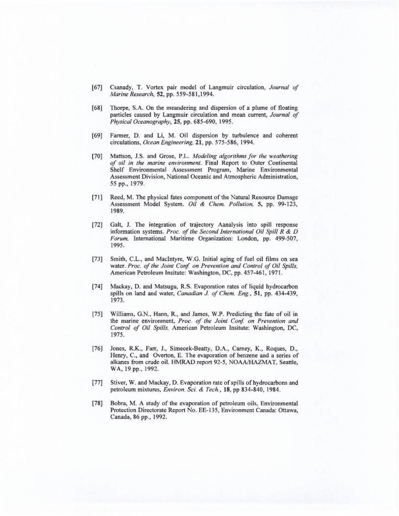
[67] Csanady, T. Vortex pair model of Langmuir circulation, Journal of Marine Research, 52, pp. 559·581 , 1994.

[68) Thorpe, S.A. On the meandering and dispe!1;ion of a plume of fl oating particles caused by Langmuir circulation and mean current, Journal of Physical Oceanography, 25, pp. 685·690, 1995.

[69J Farmer, D. and Li, M. Oil dispersion by turbulence and coherent circulations, Ocean Engineering, 21 , pp. 575-586, 1994.

[70] Mattson, J.S. and Grose, P.L. Modeling algorithms for the weathering of oil in (he marine environment. Final Report to Outer Continental Shelf Environmental Assessment Program, Marine Environmental Assessment Division, Nationa l Oceanic and Atmospheric Administration, 55 pp., 1979.

[71] Reed, M. The physical fates component of the Natural Resource Damage Assessment Model System. Oil & Chern. Pollulion, 5, pp. 99-1 23, 1989.

[72] Gall, J. The integration of trajectory Aanalysis into spill response information systems. Proc. 0/ the Second internal;onal Oil Spill R& D Forum, International Maritime Organ ization: London, pp. 499-507, 1995.

[73] Smith, c.L., and Macintyre, W.G. Initial aging of fue l oil films on sea water. Proc. of the Joint Coni on Prevention and Control of Oil Spills. American Petroleum Insitutc: Washington, DC, pp. 457-461 , 1971.

[74J Mackay, D. and Matsugu, R.S. Evaporation rates of liqu id hydrocarbon spills on land and water, Canadian J. o/Chern. Eng., 51 , pp. 434-439, 1973.

(75) Williams, G.N., Hann, R., and James, W.P. Predicting the fate of oil in the marine environment, Proc. of the Joint Con! on Prevention and Control of Oil Spills, American Petroleum Insitute: Washington, DC, 1975.

[76J Jones, R.K., Farr, J. , Simeee k-Beatty, D.A., Carney, K., Roques, D., Henry, c.. and Overton, E. The evaporation of benzene and a series of alkanes from crude oil. HMRAD report 92-5, NOAA/HAZMAT, Seattle, WA, 19pp., 1992.

[77J Stiver, W. and Mackay, D. Evaporation rate of spills ofhydrocarbons and petroleum mixtures, Environ. Sci. & Tech., 18, pp 834-840, 1984.

[78J Bobra, M. A study of the evaporation of petroleum oils, Environmental Protection Directorate Report No. EE- 135, Environment Canada: Ottawa, Canada, 86 pp., 1992.

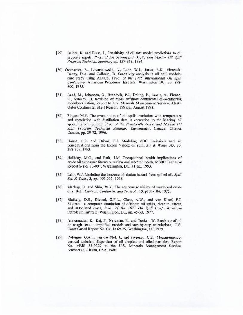
[79] BeloTe, R. and Buist, J. , Sel1sitivity of oil fate model predictions to oil property inputs, Pr()(.:. of the Seventeenth Arctic and Marine Oil Spill Program Technical Seminar, pp. 837-848, 1994.

[80J Overstreet, R., Lewandowski , A., Lehr, W.J., Jones, R.K., Simecek­Beatty, D.A. and Calhoun, D. Sensitivity analysis in oil spill models, case study using ADIOS, Proc. of the 1995 International Oil Spill Conference, American Petroleum Institute: Washington DC, pp. 898-900, 1995.

[81) Reed, M., Johansen, 0 ., Brandvik, PJ., Daling, P., Lewis, A., Fiocco, R., Mackay, D. Revision of MMS offshore continental oil-weathering model :evaluation, Repon to U.S. Minerals Management Service, Alaska Outer Continental Shelf Regi on, 199 pp., August 1998.

[821 Fingas, M.F. The evaporation of oil spills: variation with temperature and correlation with d istillation data, a correction to the Mackay oil spreading fonnulation , Proc of the Nine/eenth Arctic and Marine Oil Spill Program Technical Seminar, Environment Canada: Ottawa, Canada, pp. 29-72,1996.

[83) Hanna, S.R. and Drivas, PJ. Modeling VOC Emissions and air concentrations from the Exxon Valdez oil spill, Air & Waste ,43, pp. 298-309, 1993.

[84} Holliday, M.G., and Park, 1.M. Ckcupational health implications of crude oil exposure: literature review and research needs, MSRC Technica[ Repon Series 93-007, Washington, DC, 31 pp., 1993.

[85] Lehr, W.J. Modeling the benzene inhalation hazard from spilled oi l, Spill Sci. & Tech. , 3, pp. 199-202, 1996.

[861 Mackay, D. and Shiu, W.Y. The aqueous solubility of weathered crude oils, Bull. Environ. Contamin. and Toxicol. , 15, pI01-l04 , 1975.

[87} Blaikely, D.R., Dietzel, G.F.L., Glass, A.W., and van Kleef, PJ. Sliktrac - a computer simulation of offshore oil spills, cleanup, effect, and associated costs, Proc. of the 1977 Oil Spill Coni, American Petroleum Institute: Washington, DC, pp. 45 -53, 1977.

[88] Aravamudan, K., Raj, P., Newman, E., and Tucker, W. Break up of oil on rough seas - simplified models and step-by-step calculations, U.S. Coast Guard Rcpon No. CG-D-69-79, Washington, DC,1979.

[89] Delvigne, G.A.L, van der Stel, 1., and Sweeney, C.E. Measurement of vertical turbulent dispersion of oil droplets and oiled panicles, Report No. MMS 86-0029 to the U.S. Minerals Management Service, Anchorage, Alaska, USA, 1986.

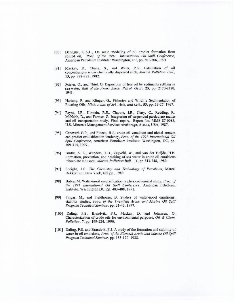
[90] Delvigne, OAL., On scale modeling of oil droplet fonnation from spilled oil, Proc. of the 1991 International Oil Spill Conference, American Petroleum Insti tute : Washington, DC, pp. 501-506, 1991 .

[91] Mackay, D., Chang, S., and Wells, P.O. CaJculalion of oil concentrations under chemically dispcrsed slick, Marine Poilution Bull. , 13, pp 278-283,1 982.

[92] Poirier, 0., and Thiel, G. Deposition of free oil by sediments settli ng in sea water, Bull of the Amer. Assoc. Petrol. Ceol., 25, pp. 2170-2180, 1941.

[93] Hartung, R. and Klinger, G., Fisheries and Wildlife Sedimentation of Floating Oils, Mich Acad. of Sci. , Arts, and Lell. , 53, pp. 23-27, 1967.

[94] Payne, J.R., Kirstein, B.E., Clayton, JR., Clary, C , Redding, R. McNabb, D., and Farmer, G. Intcgration of suspended particulate matter and oil transportation study. Final report, Report No. MMS 87-0083, U.S. Minerals Management Service: Anchorage, Alaska, USA, 1987.

[95J Cancveri, G.P., and Fiocco, RJ., crude oil vanadium and nickel content can predict emulsifi cation tendency, Proc. of the 1997 International Oil Spill Conference, American Petroleum Institute: Washington, DC, pp. 309-3 14, 1997.

[96] Bridie, A. L., Wanders, T.H .• Zegveld, W., and van der Heijde, H.B. Fonnation, prevention, and breaking of sea water in crudc oil emulsions 'chocolate mousses', Marine Pol/ution Bul/., 11, pp 343-348, 1980.

[97] Speight, lO. The Chemistry and Technology of Petroleum, Marcel Dekker Inc.: New York, 498 pp., 1980.

[98J Bobra, M. Water-in-oil emulsification: a physicochemical study, Proc. of the 1991 International Oil Spill Conference, American Petroleum Institute: Washington DC, pp. 483-488, 1991.

[99] Fingas, M., and Fieldhouse, B. Studies of water-in-oil emulsions: stability studies. Proc. of the Twentieth Arctic and Marine Oil Spill Program Technical.')'eminar, pp. 21-42, 1997.

L100] Daling, P.S., Brandvik, P.J ., Mackay, D. and Johansen, O. Characterization of crude oils for environmental purposes, Oil & Chern. Pol/ution, 7, pp. 199-224, 1990.

[101] Daling, P.S. and Brandvik, PJ. A study of the fonnation and stability of water-in-oi l emulsions, Proc. of the Eleventh Arctic and Marine Oil Spill Program Technical Seminar, pp. 153-170, 1988.

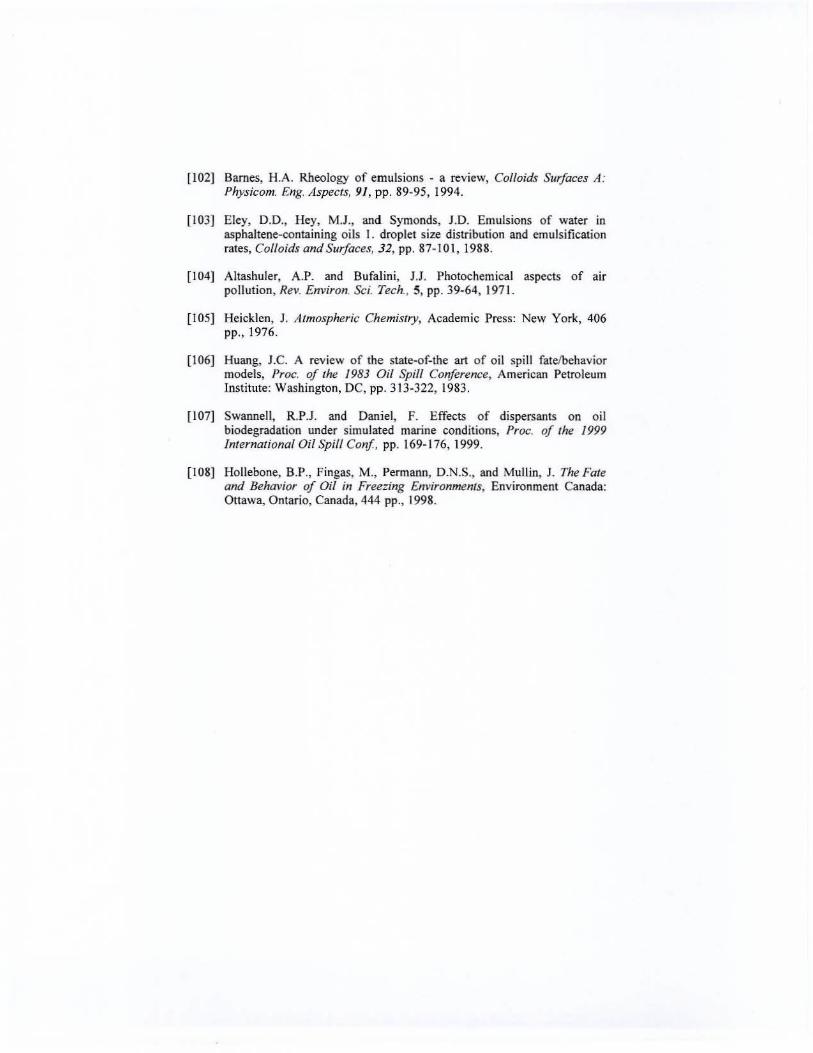
[102] Barnes, H.A. Rheology of emulsions - a review, Colloids Surfaces A: Physicom. Eng. Aspects, 91, pp. 89-95, 1994.

[l 03} Eley, D.O., Hey. M.J., and Symonds, 1.0. Emulsions of water in asphaltene-containing oils I. droplet size distribution and emulsification rates, Colloids and Surfaces, 32, pp. 87-101, 1988.

[104] Altashuler, A.P. and Bufalini, lJ. Photochemical aspects of air pollution, Rev. Environ. Sci. Tech , 5, pp. 39-64,197 1.

[105] Heicklcn, J, Atmospheric Chemistry, Academic Press: New York, 406 pp., 1976.

[1 061 Huang, J.C. A review of the state-of-the art of oil spill fate/behavior models, Proc. of the 1983 Oil Spill Conference, American Petroleum Institute: Washington, DC, pp. 313-322, 1983.

(107) Swannell, R.PJ . and Daniel, F. Effects of dispersants on oil biodegradation under simulated marine conditions, Proc. of the 1999 International Oil Spill Con!. pp. 169-1 76, 1999.

(108J Hollebone, B.P., Fingas, M., Perm ann, D.N.S., and Mullin, J. The Fate and Behavior of Oil in Freezing Environments, Environment Canada: Onawa, Onlario, Canada, 444 pp., 1998.