OIL PRICE FORECAST USING Noll PROBABILISTIC PROJECTION · PDF file... we must turn to a...

APPEA Journal 2011—411

N. MoriartyArchimedes Financial Planning3/1315 Gympie RoadAspley QLD [email protected]

ABSTRACT

Accurate forecasts for medium-term commodity prices are essential for resource companies committing to large capital expenditures. The inaccuracy of conventional fore-casting methods is well known because they tend to be extrapolations of the current price trend. The inevitable reversal catches many by surprise.

This paper demonstrates that medium-term (2–5 years) commodity prices are not strongly linked to economic health and commodity demand-supply, but are instead inversely controlled by supply-demand for the United States dollar (USD) and consequent valuation. P90, P50 and P10 projection bounds for future valuation of the USD are presented based on the successful probabilistic techniques of the petroleum exploration industry.

This allows probabilistic projections for the oil price, which is inversely related to the USD valuation. I show that the USD is significantly undervalued at present. Probabilistic projection of the USD valuation indicates that likely appreciation will put downward pressure on commodity prices for the next 2–5 years. If the USD prem-ise is correct, likely appreciation of the dollar during the next 2–5 years will hold stable, or even decrease, oil price to around USD $50 BBL. This is a contrary expectation to most forecasts—one which, if it eventuates, should give cause for reflection before committing to large capital expenditures.

Further investigation could examine the extent to which the USD valuation can be modelled as a fractal phenom-enon. If so, it would mean the USD valuation is not driven by conventional economic fundamentals; instead, it is a semi-random number series with serial correlation. If true, probabilistic forecasts of the USD can be significantly improved, hence that of medium-term commodity prices.

KEYWORDS

Oil price forecast, commodity price forecast, Econophys-ics, probabilistic forecast, US dollar, fractal phenomenon.

INTRODUCTION

Accurate forecasting of medium-term oil prices is es-sential when considering commitment to large capital ex-penditures. Commodity price forecasts are often extrapola-tions of the current trend, which works fine until a turning point occurs. Forecasters can do a lot better than this if predictions are controlled by accurate probabilistic bounds.

Conventional economic theory presumes prices of con-sumable commodities, such as oil, are primarily set by the interaction of commodity supply and demand. The price of another commodity, gold, is presumed to vary in accordance with expectations of inflation and status of global geopolitics. Since different factors affect oil and gold prices, there should not be a strong correlation between their price changes. The American Geological Institute (2008) compared the USD price for spot oil and gold during 2000–08 (Fig. 1). The conclusion was that the price of these commodities was inversely controlled by valuation strength of USD, since the ratio of oil price to gold price was stable. In this paper, I extend examination to the longer time period, of since 1980, with a statistical analysis of the USD monthly valuation changes to enable probabilistic projection of the USD and hence (inversely) prediction of the oil price.

Factors that conventional economic theory suggest affect consumable commodities, such as commodity demand and supply, are compared with changes in the oil price. I con-sider whether there are two supply-demand mechanisms

OIL PRICE FORECAST USING PROBABILISTIC PROJECTION OF ThE

UNITED STATES DOLLAR

Lead authorNoll

Moriarty

Figure 1. Relationship between oil and gold prices during 2000–08.

412—APPEA Journal 2011

N. Moriarty

in play—for commodities and for the USD. The lack of a significant correlation of commodity price with commodity supply-demand asks the question: what is the predominant control on changes of the oil price?

I examine the strength of the link between USD valu-ation and oil price. If the valuation of the USD is a major effect and we wish to forecast oil price, factors that affect the USD need to be understood. I examine the impact that conventional economic factors (such as strength of economy and debt-to-GDP), have on the valuation of the USD. If these factors are not reliably predictive, we must turn to a probabilistic projection for the USD valuation (of which, the inverse prediction encompasses bounds for the future price of oil) using statistical techniques to pre-dict probabilistic bounds for the oil price. Conventional probabilistic methods require definition of many variables, all presumed to have an influence on oil price. Empirical analysis calls into question the relevance of these variables. The approach used in this paper avoids this pitfall, using only the USD valuation.

The modelling in this paper is a low level example of econophysics. This is an exciting new academic field that applies concepts of statistical physics to financial time series to gain new insights into the behaviour of financial markets. In the study of economic systems, it is usually impossible to develop equations for microscopic interac-tions of all interacting entities. The empirical techniques of statistical physics, however, allow examination and probabilistic predictions of the system as a whole without knowing the individual behavior of all contributing agents. For the interested reader, excellent initial references to econophysics are Mantegna and Stanley (2000) and Voit (2005). A compelling example of econophysics applied to stock markets is seen in Sornette (2003).

These predictions will be helpful adjuncts to the more conventional forecasting techniques, particularly when decisions relating to large capital expenditures rely on a high probability of at least a minimum oil price. Being able to put objective probabilistic bounds is a valuable reality check on human emotions.

METHOD

To investigate the link between commodity prices and the USD valuation, I examine both oil and gold prices, since it is commonly regarded that different factors control their prices. Time series data for this paper are sourced from: the Federal Reserve Bank of St Louis West Texas Interme-diate Spot Oil Price (code: OILPRICE); inflation (code: CPIAUCSL); real GDP quarterly percentage change (code: GDPC1); and, USD Trade Weighted Exchange Index Major Currencies (code: TWEXMMTH). Gold price is sourced from the Reserve Bank of Australia, statistical table F12.

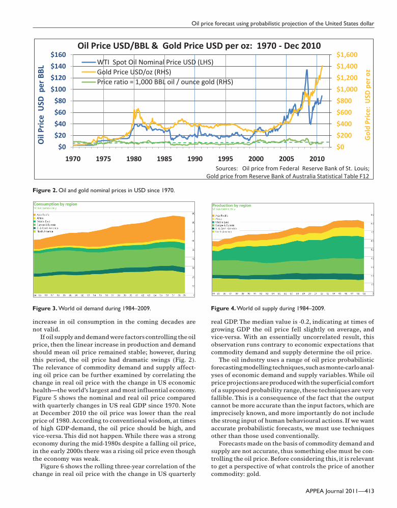
Monthly nominal USD prices of oil and gold since 1970 are shown in Figure 2. During the 1970s, there was an unequivocal link between USD valuation and commodity prices. Prices of most commodities had step changes as the USD depreciated while it moved off the gold standard.

Inflation was rampant after the US Government printed money to fund the Vietnam war, forcing the Organisation of the Petroleum Exporting Countries (OPEC) to raise prices to protect the value of oil exports. At the end of the 1970s, speculators such as the Hunt Brothers manipulated prices of precious metals, particularly silver, which had a knock-on effect on the price of gold. The sudden jumps in commodity prices was a sign of a loss of confidence in the USD, demonstrating a strong inverse link between USD valuation and commodity prices at this time.

Fearing the emergence of a gold-based currency not under its central bank control, the US Government pro-tected the USD by changing the trading rules of the New York Mercantile Exchange and Commodity Exchange, Inc (COMEX). These changes had the desired effect, with the USD beginning a strong appreciation, which culminated in an all-time high in 1985.

In this paper, the analysis of oil prices starts from 1980, since volatility of commodity prices was lower then than in the previous decade. Prices of oil and gold fell during 1980–85. In 1986, another step change occurred in the oil price as a delayed consequence of OPEC not reducing production after the 1981–82 world recession. Both com-modities had fairly stable, but slightly falling, nominal prices between the late 1980s to late 1990s.

The oil price has another step increase in the late 1990s, but prices of both commodities fell to a low around 2002. Prices then rose strongly, particularly after 2006. During the global financial crisis, however, commodity prices fell, in particular the price of oil. Gold continues to maintain stratospheric prices while the oil price has recovered only some of its loss.

This raises the question: where next for oil prices?

CONVENTIONAL FORECASTING COMMODITY PRICES

Forecasting oil price

Oil price forecasts typically consider the interplay of oil supply (existing and new production) and oil demand (global economic activity). Therefore, it is pertinent to get a perspective on oil demand and supply over the last few decades.

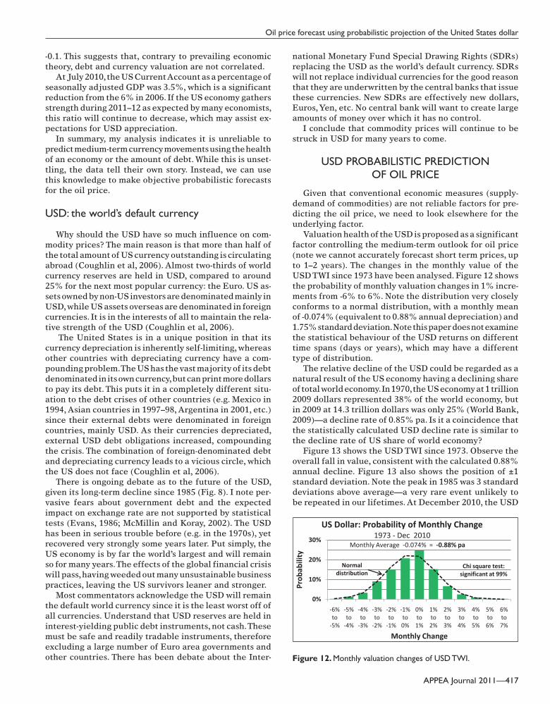
Every year, BP publishes a statistical review of world energy usage and reserves (BP, 2010). The 2010 review presented world oil demand (Fig. 3) and supply (Fig. 4) for the period 1984–2009. The BP review shows that world oil supply and demand during 1984–2009 increased at a constant increment each year, from 58 MMBBL/day in 1984 to 80 MMBBL/day in 2009—equivalent to about 2,700 BBL per day. The observation that oil consumption increased linearly is not the commonly expected exponential increase caused by population increase. My explanation for the linear increase is as the price of a commodity increases, industry and people are forced to become more efficient to contain costs. Thus Malthusian fears of an exponential


Oil price forecast using probabilistic projection of the United States dollar

increase in oil consumption in the coming decades are not valid.

If oil supply and demand were factors controlling the oil price, then the linear increase in production and demand should mean oil price remained stable; however, during this period, the oil price had dramatic swings (Fig. 2). The relevance of commodity demand and supply affect-ing oil price can be further examined by correlating the change in real oil price with the change in US economic health—the world’s largest and most influential economy. Figure 5 shows the nominal and real oil price compared with quarterly changes in US real GDP since 1970. Note at December 2010 the oil price was lower than the real price of 1980. According to conventional wisdom, at times of high GDP-demand, the oil price should be high, and vice-versa. This did not happen. While there was a strong economy during the mid-1980s despite a falling oil price, in the early 2000s there was a rising oil price even though the economy was weak.

Figure 6 shows the rolling three-year correlation of the change in real oil price with the change in US quarterly

real GDP. The median value is -0.2, indicating at times of growing GDP the oil price fell slightly on average, and vice-versa. With an essentially uncorrelated result, this observation runs contrary to economic expectations that commodity demand and supply determine the oil price.

The oil industry uses a range of oil price probabilistic forecasting modelling techniques, such as monte-carlo anal-yses of economic demand and supply variables. While oil price projections are produced with the superficial comfort of a supposed probability range, these techniques are very fallible. This is a consequence of the fact that the output cannot be more accurate than the input factors, which are imprecisely known, and more importantly do not include the strong input of human behavioural actions. If we want accurate probabilistic forecasts, we must use techniques other than those used conventionally.

Forecasts made on the basis of commodity demand and supply are not accurate, thus something else must be con-trolling the oil price. Before considering this, it is relevant to get a perspective of what controls the price of another commodity: gold.

$0

$200

$400

$600

$800

$1,000

$1,200

$1,400

$1,600

$0

$20

$40

$60

$80

$100

$120

$140

$160

1970 1975 1980 1985 1990 1995 2000 2005 2010

Gol

d Pr

ice:

USD

per

oz

Oil

Pric

e U

SD p

er B

BLOil Price USD/BBL & Gold Price USD per oz: 1970 - Dec 2010

WTI Spot Oil Nominal Price USD (LHS)Gold Price USD/oz (RHS)Price ratio = 1,000 BBL oil / ounce gold (RHS)

Sources: Oil price from Federal Reserve Bank of St. Louis; Gold price from Reserve Bank of Australia Statistical Table F12

Figure 2. Oil and gold nominal prices in USD since 1970.

Figure 3. World oil demand during 1984–2009.

Figure 4. World oil supply during 1984–2009.


N. Moriarty

Forecasting gold price

The price of gold is considered to be primarily controlled by concerns about inflation and geopolitical events. By comparing gold price changes with inflation and noting times of major geopolitical concern, the accuracy of this link can be examined.

Figure 7 shows the nominal and real gold price compared with US rolling annual inflation. While there is some cor-respondence between gold price and inflation, the rolling five-year correlation averages 0.2, indicating a weak link at best. Note that times of major geopolitical concern did not translate into consistent increases in gold price, thus something else must be controlling the gold price.

COMMODITY PRICES—LINKED BY US DOLLAR VALUATION

Since 1980, the USD price ratio of 1 oz gold divided by 1,000 BBL oil has been stable at 73 ± 25 (Fig 2). This suggests a common link between the pricing of these very different commodities. Conventional wisdom is that oil prices are set primarily by the interaction of oil supply and demand, whereas gold price is influenced by inflation rates and the status of the global geopolitical situation. Since different factors affect base metals and gold prices,

there should not be a strong link between prices. The ratio of their prices would be expected to vary widely at times, yet this has not happened. This indicates that USD valu-ation changes may be a strong control on medium-term prices of oil and gold. It is accepted that momentum and speculators control short-term price movements, but even-tually reality returns to pricing.

To examine the USD valuation effect on commodity prices, consider the USD Trade Weighted Index (TWI). This is the weighted average of the exchange rates of home and foreign currencies, with the weight for each foreign country equal to its share in trade with the home country. There are several measures of the TWI, with the main one being the Broad Index, which includes all countries whose imports or exports exceed 0.5% of US economy. These weights change every year as bilateral economies strengthen and weaken. A country’s TWI is the best mea-sure of the health of its currency.

In this paper, I use a subset called the Major Curren-cies Trade Weighted Index (Fig. 8) since these currencies generally trade widely in liquid financial markets and can be used to gauge financial market pressures on the USD. In 2010, contributors to the USD TWI Major Currencies Index were from a 36.6% Euro area, 30.2% Canada, 17.0% Japan, 8.5% United Kingdom, 3.2% Switzerland, 2.6% Australia and 2.0% Sweden (US Federal Reserve, 2010). Observe the USD TWI had broad trends. It increased during 1980–85; decreased during 1986–88; was stable during 1989–96; increased during 1997–2002; and, decreased after 2003.

Figure 9 shows oil and gold USD prices, with gold price plotted as a one-tenth ounce, and the USD TWI plotted on an inverted right-hand scale. Observe the close inverse relationship between the USD TWI and commodity prices, especially with gold during 1988–2005. Note between the step changes for price of oil—a decrease in 1986 and an increase in 1999—that the oil price changes inversely tracked changes in USD valuation. It is noted that there has been a disconnection between commodity prices and the USD in the past, but after some years a connection was re-established based on the USD valuation.

During 2006–08, euphoria over China’s industrialisa-tion caused a spike in commodity prices. The oil price has since reversed much of this spike, while gold appears to be overpriced based on USD currency considerations. The USD TWI suggests a more appropriate gold price now is about $500 per ounce, with oil at about $50 BBL.

The inverse relationship for USD TWI and commodity prices suggests parties setting the commodity prices sought a stable return: as the USD depreciated, prices of com-modities rose commensurately, and vice-versa. I suggest there are two supply-demand mechanisms in play: supply-demand for commodities, but also quite an independent supply-demand for the USD itself. Simply only considering supply-demand for commodities is flawed, because it ig-nores the other demand function. Had the supply-demand for commodities remained constant but the supply of USD increased, then commodity prices should rise in apparent USD terms, while really remaining constant.

-4.0

-3.0

-2.0

-1.0

0.0

1.0

2.0

3.0

4.0

$0

$20

$40

$60

$80

$100

$120

$140

$160

1970 1980 1990 2000 2010

Real

GD

P Q

uart

erly

Cha

nge

WTI

Spo

t O

il P

rice

(U

SD)

Real Oil Price & US Real GDP Change: 1970 - Dec 2010

US Real GDP Quarterly % Change (RHS) WTI Spot Oil Nominal Price USD (LHS)Oil Price (Real USD)

Source: Federal Reserve Bank of St. Louis GDPC1

Figure 5. Oil price (nominal and real) and US real GDP.

-1.0

-0.5

0.0

0.5

1.0

1975 1980 1985 1990 1995 2000 2005 2010

Corr

elat

ion

Coef

fici

ent

Real Oil Price Change Vs. Real GDP Change3-Year Rolling Correlation

Median = -0.22

Figure 6. Rolling correlation of real oil price and US real GDP.



-5%

0%

5%

10%

15%

20%

25%

30%

35%

40%

45%

$0

$200

$400

$600

$800

$1,000

$1,200

$1,400

$1,600

$1,800

$2,000

1980 1985 1990 1995 2000 2005 2010

US

Rol

ling

Ann

ual I

nfla

tion

Gol

d P

rice

U

SD p

er o

z

Gold Price & Inflation: 1980 - 2010

Gold Price Nominal USD per oz (lhs) Gold Price Real USD per oz (lhs)US Rolling Annual Inflation (rhs)

Sources: Federal Reserve Bank of St. Louis; Reserve Bank Australia Statistical Table F12

Gulf War

Mexico;Bond crisis

Russia default;Long term Cap Man't

Argentina default

Global Financial

Crisis

Figure 7. Gold price versus inflation and geopolitical events.

F12HIST.XLS

50

100

150

200

250

300USD Trade Weighted Index: Major Currencies 1980 - Dec 2010

Source: Reserve Bank of Australia Statistical Table F12

Page 1

0

50

100

150

200

250

300

1980 1985 1990 1995 2000 2005 2010

USD Trade Weighted Index: Major Currencies 1980 - Dec 2010

Euro * 100 Canadian $ * 100 Japanese Yen UK Pound * 100 Swiss Franc * 100 AUD * 100 USD Trade Weighted Index Gold (USD per tenth-oz)

Source: Reserve Bank of Australia Statistical Table F12

Figure 8. USD Trade Weighted Index—major currencies.


N. Moriarty

What controls USD valuation?

If the USD valuation and medium-term commodity prices have an inverse relationship, then forecasts for commodity prices should be based on future expecta-tions of the USD currency movement. To do this, we need an understanding of the magnitude and length of past appreciation and depreciation movements of the USD, compared to prevailing economic factors such as United States GDP and debt.

Figure 10 shows the quarterly change in United States real GDP since 1970 and the USD TWI cumulative move-ments since 1973. Conventional economic wisdom is that when an economy is strong, so should its currency be, and vice-versa. Note there is not a strong link between the economy health and currency valuation (in fact, the aver-age correlation is 0.1). Therefore, based on views of the health of the US economy, confident predictions of USD future valuation are suspect, though superficially plausible.

Next consider whether the amount of US debt controls the valuation of the USD. To examine this, consider the US Current Account, which is the difference in import/export for trade in goods and services, and earnings on investments. Essentially, an increasing Current Account means that the amount of debt is decreasing, and vice-versa. The Current Account is expressed as a percentage of GDP, which is the most appropriate way to view chang-ing debt since the value of the asset—the economy—is equally important. An increasing Current Account as a percentage of GDP means debt is decreasing (in theory, currency should appreciate) and vice-versa.

Figure 11 shows USD cumulative monthly valuation compared with quarterly values of United States Current Account, as a percentage of seasonally adjusted GDP. Note there is not a strong relationship between decreasing debt and rising currency valuation, or increasing debt and de-creasing currency valuation. For example, the USD appreci-ated strongly while the Current Account deficit increased

during 1982–85 and 1995–2002. During the early 1980s, the US federal government operated with a large deficit and printed money, which raised investor fears about infla-tion. It is relevant to note conventional economic beliefs of impact of government debt on US dollar valuation are not supported by statistical tests (Evans, 1986; McMillin and Koray, 2002). The rolling five-year correlation between Current Account as a percentage of GDP and USD TWI is

-50

-30

-10

10

30

50

70

90

110

130$0

$10$20$30$40$50$60$70$80$90

$100$110$120$130$140$150

1980 1985 1990 1995 2000 2005 2010

USD

Tra

de W

eigh

ted

Inde

x

Oil

Pric

e BB

L &

Gol

d Pr

ice

USD

per

tent

h-oz

USD Trade Weighted Index & Oil, Gold Prices: 1980 - 2010Gold USD per tenth-oz (lhs)

West Texas Intermediate Spot Oil USD (lhs)

USD Trade Weighted Index (rhs inverted scale)


Figure 9. USD valuation compared with commodity prices.

-3.0

-2.0

-1.0

0.0

1.0

2.0

3.0

4.0

-60%

-40%

-20%

0%

20%

40%

60%

80%

1970 1980 1990 2000 2010

Real

GD

P Q

uart

erly

Cha

nge

USD

D

epre

ciat

ion

/A

ppre

ciat

ion

USD Valuation Change & Real GDP: 1970-2010

US Real GDP Quarterly % Change (RHS) USD Depreciation (LHS)USD Appreciation (LHS)

Source: Federal Reserve Bank of St. Louis TWEXMMTH, GDPC1

Figure 10. USD valuation changes compared with strength of the US economy.

-9.0%

-6.0%

-3.0%

0.0%

3.0%

6.0%

9.0%

-60%

-40%

-20%

0%

20%

40%

60%

1970 1980 1990 2000 2010 CA a

s %

GD

P (S

easo

nally

Adj

uste

d)

USD

Dep

rec

iati

on /

App

reci

atio

n

USD Valuation vs. Current Account as Percent of Real GDP

Current Account as Percent Real GDP quarterly (RHS)USD Appreciation (LHS)USD Depreciation (LHS)

Source: Federal Reserve St Louis NEFTI, TWEXMMTH

1970 - Dec 2010

Figure 11. USD valuation changes compared with changing debt.



-0.1. This suggests that, contrary to prevailing economic theory, debt and currency valuation are not correlated.

At July 2010, the US Current Account as a percentage of seasonally adjusted GDP was 3.5%, which is a significant reduction from the 6% in 2006. If the US economy gathers strength during 2011–12 as expected by many economists, this ratio will continue to decrease, which may assist ex-pectations for USD appreciation.

In summary, my analysis indicates it is unreliable to predict medium-term currency movements using the health of an economy or the amount of debt. While this is unset-tling, the data tell their own story. Instead, we can use this knowledge to make objective probabilistic forecasts for the oil price.

USD: the world’s default currency

Why should the USD have so much influence on com-modity prices? The main reason is that more than half of the total amount of US currency outstanding is circulating abroad (Coughlin et al, 2006). Almost two-thirds of world currency reserves are held in USD, compared to around 25% for the next most popular currency: the Euro. US as-sets owned by non-US investors are denominated mainly in USD, while US assets overseas are denominated in foreign currencies. It is in the interests of all to maintain the rela-tive strength of the USD (Coughlin et al, 2006).

The United States is in a unique position in that its currency depreciation is inherently self-limiting, whereas other countries with depreciating currency have a com-pounding problem. The US has the vast majority of its debt denominated in its own currency, but can print more dollars to pay its debt. This puts it in a completely different situ-ation to the debt crises of other countries (e.g. Mexico in 1994, Asian countries in 1997–98, Argentina in 2001, etc.) since their external debts were denominated in foreign countries, mainly USD. As their currencies depreciated, external USD debt obligations increased, compounding the crisis. The combination of foreign-denominated debt and depreciating currency leads to a vicious circle, which the US does not face (Coughlin et al, 2006).

There is ongoing debate as to the future of the USD, given its long-term decline since 1985 (Fig. 8). I note per-vasive fears about government debt and the expected impact on exchange rate are not supported by statistical tests (Evans, 1986; McMillin and Koray, 2002). The USD has been in serious trouble before (e.g. in the 1970s), yet recovered very strongly some years later. Put simply, the US economy is by far the world’s largest and will remain so for many years. The effects of the global financial crisis will pass, having weeded out many unsustainable business practices, leaving the US survivors leaner and stronger.

Most commentators acknowledge the USD will remain the default world currency since it is the least worst off of all currencies. Understand that USD reserves are held in interest-yielding public debt instruments, not cash. These must be safe and readily tradable instruments, therefore excluding a large number of Euro area governments and other countries. There has been debate about the Inter-

national Monetary Fund Special Drawing Rights (SDRs) replacing the USD as the world’s default currency. SDRs will not replace individual currencies for the good reason that they are underwritten by the central banks that issue these currencies. New SDRs are effectively new dollars, Euros, Yen, etc. No central bank will want to create large amounts of money over which it has no control.

I conclude that commodity prices will continue to be struck in USD for many years to come.

USD PROBABILISTIC PREDICTION OF OIL PRICE

Given that conventional economic measures (supply-demand of commodities) are not reliable factors for pre-dicting the oil price, we need to look elsewhere for the underlying factor.

Valuation health of the USD is proposed as a significant factor controlling the medium-term outlook for oil price (note we cannot accurately forecast short term prices, up to 1–2 years). The changes in the monthly value of the USD TWI since 1973 have been analysed. Figure 12 shows the probability of monthly valuation changes in 1% incre-ments from -6% to 6%. Note the distribution very closely conforms to a normal distribution, with a monthly mean of -0.074% (equivalent to 0.88% annual depreciation) and 1.75% standard deviation. Note this paper does not examine the statistical behaviour of the USD returns on different time spans (days or years), which may have a different type of distribution.

The relative decline of the USD could be regarded as a natural result of the US economy having a declining share of total world economy. In 1970, the US economy at 1 trillion 2009 dollars represented 38% of the world economy, but in 2009 at 14.3 trillion dollars was only 25% (World Bank, 2009)—a decline rate of 0.85% pa. Is it a coincidence that the statistically calculated USD decline rate is similar to the decline rate of US share of world economy?

Figure 13 shows the USD TWI since 1973. Observe the overall fall in value, consistent with the calculated 0.88% annual decline. Figure 13 also shows the position of ±1 standard deviation. Note the peak in 1985 was 3 standard deviations above average—a very rare event unlikely to be repeated in our lifetimes. At December 2010, the USD

0%

10%

20%

30%

-6% to

-5%

-5% to

-4%

-4% to

-3%

-3% to

-2%

-2% to

-1%

-1% to 0%

0% to 1%

1% to 2%

2% to 3%

3% to 4%

4% to 5%

5% to 6%

6% to 7%

Prob

abili

ty

Monthly Change

US Dollar: Probability of Monthly Change1973 - Dec 2010

Monthly Average -0.074% = -0.88% pa

Normal distribution

Chi square test:significant at 99%

Figure 12. Monthly valuation changes of USD TWI.


N. Moriarty

was nearing 1 standard deviation below median. This sup-ports the assertion that the USD is presently undervalued and oversold.

This paper presents forward probabilistic modelling of the USD TWI monthly series. The procedure uses only the TWI index since 1973 (no other variables) and requires an input of only the starting point— no matter how far above or below average it is—and the range around this starting point that is to be examined. For example, given a start-ing point around 1 standard deviation below average, the TWI percentage changes over the following 1–5 years are determined with starting points in the range from around 0.5 to 1.5 standard deviations below average. The results are ranked from smallest to largest percent change, then expressed as probabilities from P90 (90% certain the TWI will equal or exceed the P90 value), P50 and P10 valuations for the USD. Given these results, five-year probabilistic projections for the USD can be made.

Back-tested examples of this probabilistic modelling are shown for two cases: TWI for 1995–99 (Fig. 14) and 2000–04 (Fig. 15). The Figure 14 starting point is near 1 standard deviation below average (similar to the valuation at Dec. 2010). The subsequent TWI valuations are mostly bound by the predicted P90 and P10 limits and averaged around P50. The modelling correctly predicted the TWI would increase over the next five years, an example of mean reversion. The Figure 15 starting point is near 1 standard deviation above average. The subsequent TWI valuations are mostly bound by the predicted P90 and P10 limits, but only reached the P50 value after five years (this result is a consequence of serial correlation, see the later section on the possibility of the TWI as a fractal phenomenon). The probabilistic modelling correctly predicted the tim-ing of the subsequent TWI decrease. This gives a sign that

60708090

100110120130140150

Dec

-72

Dec

-74

Dec

-76

Dec

-78

Dec

-80

Dec

-82

Dec

-84

Dec

-86

Dec

-88

Dec

-90

Dec

-92

Dec

-94

Dec

-96

Dec

-98

Dec

-00

Dec

-02

Dec

-04

Dec

-06

Dec

-08

Dec

-10

Dec

-12

Dec

-14

USD Trade Weighted Index 1973 - Dec 2010

USD Trade Weighted Index USD Average TWI1 St Dev below average 1 St Dev above average

Source: Federal Reserve Bank of St Louis TWEXMMTH, Trade Weighted Exchange Index:

Average decline 0.88% pa

P10

P90

P50

USD probabilistic

forecast range

Figure 13. USD valuation predictions over the next five years with 90%, 50% and 10% confidence.

70

80

90

100

110

120

Dec

-94

Dec

-95

Dec

-96

Dec

-97

Dec

-98

Dec

-99

USD

Tra

de W

eigh

ted

Inde

x

USD Trade Weighted Index - Probabilistic Forecast 1995-9


Source: Federal Reserve Bank of St Louis TWEXMMTH, Trade Weighted Exchange Index: P10

P90

P50

Figure 14. USD probabilistic predictions for the period 1995–99.

60

70

80

90

100

110

120

Dec

-99

Dec

-00

Dec

-01

Dec

-02

Dec

-03

Dec

-04

USD

Tra

de W

eigh

ted

Inde

x

USD Trade Weighted Index - Probabilistic Forecast 2000-4


Source: Federal Reserve Bank of St Louis TWEXMMTH, Trade Weghted Exchange Index:

P10

P90

P50

Figure 15. USD probabilistic predictions for the period 2000–04.



the modelling technique has validity; it is essentially an exercise in estimating timing and rate of mean reversion.

Turning now to the present, Figure 13 also shows pre-dicted valuations for the TWI during 2010–14. These pre-dictions were made in December 2009 for my clients. The USD initially appreciated along the P10 path, but has since fallen to around the P50 projection. Observe on a P50 basis, the USD is likely to appreciate beyond its average value around 2013.

Figure 16 shows the USD TWI for the period 2000–10 with the probabilistic projections from Figure 13 both plotted with an inverse scale, and the commodity prices of Figure 9. Note the present massive disconnection between USD and commodity prices. The probabilistic predictions of USD valuation suggest a realistic value for oil to be around $50 BBL, and $500 per oz for gold during the next few years. If true, the momentum holding up commodity prices will likely reverse rapidly sometime in the next year or so. A pointer as to when this may occur is to watch the US Federal Reserve interest rates—when these start rising, is a signal the US economy is improving.

Disconnections between USD valuation and commod-ity prices have occurred in the past, but eventually the USD regained its dominance in each case. Therefore, I sug-gest that claims it is different this time—that commodity prices will maintain their strong upward mometum due

to Chinese demand—should be treated with caution. I have demonstrated that demand is not a reliable control on oil price (Fig. 5). In addition, although the world has seen large industrialisations over the last century (United States, Europe post-WWII, and Japan, etc.), the real prices of commodities have decreased overall. For example, the real price of oil is now similar to the average price around 1980, despite a large increase in demand (Fig. 5). Note the price of the bellwether commodity, copper, progressively decreased during the last century (USGS, 2009).

Peak oil: impact on oil price

Proponents of peak oil say as oil demand exceeds supply, the oil price will rise strongly, therefore decoupling from any link with the USD. I suggest that an inexorable rise in the price of oil is not a given for two reasons.

Firstly, as the oil price rises, it opens up scope for alter-native energy sources to become cost-effective and replace oil usage. The world economy has reacted to step increases in oil price over the last decades. Oil as a primary energy source for the world has reduced from 46% in 1973 to 33% in 2008 (IEA, 2008), by increased diversification of energy resources and better efficiency. Increasing oil prices will maintain the impetus to continue reducing oil consump-tion per capita.

-50-30-101030507090110130

$0$10$20$30$40$50$60$70$80$90

$100$110$120$130$140$150

2000 2002 2004 2006 2008 2010 2012 2014

USD

Tra

de W

eigh

ted

Inde

x

Oil

Pric

e BB

L &

Gol

d Pr

ice

USD

per

ten

th-o

z

USD Probabilistic Forecast for prices of Oil & Gold

Gold USD per tenth-oz (lhs)West Texas Intermediate Spot Oil USD (lhs)USD Trade Weighted Index (rhs inverted scale)


P90

P10P50

USD probabilistic forecast indicates oil & gold prices should

be much lower

Figure 16. USD predictions over the next five years and oil price.


N. Moriarty

Secondly, oil industry personnel with a historical per-spective know the ratio of reserves to production has been constant for about 40 years (Fig. 17). This indicates that the amount of oil reserves added each year continues to match the increasing consumption. It suggests any impact of peak oil will be a gradual process and not a step change because its effect will be spread over many years. Con-sumption is not an exponential growing series—instead it is linear (Fig. 3). Therefore peak oil, when it occurs, will likely have a gradual impact on long term oil prices.

Further investigation: are USD monthly returns a fractal phenomenon?

As an extension of the proposition that the USD valua-tion is a significant control on commodity prices, I propose a hypothesis for further investigation: could the USD valu-ations be modelled as a fractal phenomenon? If true, it would mean USD movements are unrelated to economic or any other fundamental analysis. This assertion will dis-concert forecasters relying on gathering tractable metrics to predict future oil price, but if true opens up scope for objective econophysics forecasting techniques.

The usual approach when predicting bi-lateral currency exchange rates is to consider economic fundamentals such as the debt-to-GDP ratio, commodity prices and interest rate differential. One example of such a study is Cayen et al (2010). While these studies have merit, the conclusions drawn are based on theoretical (therefore debatable) as-sumptions, such as that a rise in debt-to-GDP should result in currency depreciation. Figure 11 shows the opposite for the USD during 1982–85, 1988–2002, and 2006–08—not a very convincing assumption.

I have shown the USD monthly valuation returns conform to a normal distribution with a mean of -0.074%. Note a normal distribution does not necessarily imply USD returns are randomly distributed. Randomness requires variations to be independently and identically distributed (IID) with each month’s return unaffected by the previous month. Yet serial dependence is demonstrated for the USD returns, given the probability of runs of 6–8 consecutive months of positive and negative periods being higher than would be expected by random chance alone (Fig. 18). Long con-secutive runs of positive or negative monthly returns are outliers on the statistical distribution of random returns. These outliers can be predicted using the non-linear log-periodic approach (Sornette, 2003), providing a quantita-tive basis to predictions.

My hypothesis is that USD monthly returns could be modelled in a similar way to Mandelbrot’s Multifractal Model for stock market returns (Mandelbrot and Hud-son, 2004). Such an analysis would be an application of the power law methodology described by Taleb (2007). The final result has large price variations (i.e. fat tails), which are volatility clusters interspersed with more sedate intervals. If true, the USD monthly returns would have a high degree of predictability (particularly for the larger magnitude drawdowns), and be responsive to the analyti-cal econophysics techniques being successfully applied to

predicting stock market returns. These suggest the vast majority of the movements can be fitted with a so-called random walk model, but the largest movements will be predictable outliers, amenable to the analytical techniques of Sornette (2003).

Applying a fractal modelling technique to the USD would provide an objective forecast for future USD valuations and the inversely-related oil price. This would be a power-ful additional tool when making forecasts for commodity prices. Such a probabilistic USD projection methodology does not rely on conventional forecasting considerations of commodities supply and demand. Instead, it would as-sume the USD valuation can be modelled as a fractal se-ries generated from a distribution with a monthly mean of -0.074%, which has significant serial correlation. This approach will be disquieting to many who look to so-called

Figure 18. USD consecutive runs for positive and negative months.

Figure 17. World oil reserves-to-production 1985–2009. Source: BP Statistical Review 2010

0%

5%

10%

15%

20%

25%

30%

8 - 7 - 6 - 5 - 4 - 3 - 2 - 1 - 1 + 2 + 3 + 4 + 5 + 6 + 7 + 8 +

Prob

abili

ty

Consecutive Runs of Negative / Positive months

USD TWI: Consecutive +/- months 1973- Dec 2010

Actual Result

Random normal distribution



fundamental economic factors to explain, usually after the event, why the oil price had the consequent trend. We know the conventional forecasting approach is not reliable, so why not use a statistical methodology that encompasses fallible human emotions?

CONCLUSIONS

Conventional oil price forecasting techniques, such as considering oil demand and demand, are not reliable for predicting medium-term commodity prices. How many forecasters at the start of 2001, when the oil price was $25 BBL and decreasing, would have correctly forecast the subsequent strong price rise in the next five years and its timing? Note the probabilistic USD modelling (Figs 15, 16) would have correctly predicted not only would the lowest price be around the end of 2001, but also that a P50 oil price of around $40–50 BBL at the end of 2004—the price that subsequently occurred. The stratospheric prices before the global financial crisis were not predictable and not based on fundamentals such as demand. The price rise was a momentum effect, largely driven by trading banks and futures speculators (Coleman and Levin, 2006).

I contend medium-term commodity prices are mainly driven by the supply and demand of the USD, which affects its valuation. Short-term commodity price trends, such as the recent oil price surge and decline during 2006–08, are controlled not by currency, but by momentum and specula-tors. The inverse relationship for USD TWI and commod-ity prices suggests parties setting the commodity prices sought a stable return: as the USD depreciated, prices of commodities rose commensurately, and vice-versa.

Common probabilistic techniques for forecasting oil price have an inherent fallibility: relevant input parameters are not well defined (mean and distribution shape), and the link of many parameters to oil price changes is weak at best. Making monte-carlo projections, then inferring P90 and P10 bounds based on these questionable assumptions, gives decision-makers false comfort.

Commodity price forecasts should consider an objective probabilistic methodology based on USD monthly valua-tions. These returns conform to a normal distribution but are not random; instead, they have a significant measure of serial correlations with mean reversion. Using this ap-proach avoids the fallibility of commonly used probabilistic models, since the USD TWI probability bounds are inferred from only the TWI data with no other variables required. These bounds can be viewed with confidence, given the almost 40-year history of volatility in the USD.

Statistical analysis indicates the USD, measured against its TWI, suggests that the TWI is oversold as at December 2010. This opens up the significant probability that the USD will appreciate over the next several years. USD apprecia-tion should put downward pressure on commodity prices.

The probabilistic modelling in this paper indicates dur-ing the medium term (the next 2–5 years), the oil price could average around USD $50 BBL and gold could fall to around USD $500 per ounce (these prices should be increased by inflation in the coming years). The recent

large increase in gold price has the hallmarks of bubble psychology: ever increasing growth rate and an increased number of trades, both driven by prominent media cover-age and input from interested commentators. Econophysics techniques (Sornette, 2003) indicate the bubble will burst. The commodities euphoria has also affected the oil price, but not to the same extent as the price of gold. This paper has demonstrated so-called fundamentals that supposedly control the oil price are not determinants of the price, and that reality will set in due course.

Predicting that commodity prices will not rise signifi-cantly over the medium term is contrary to most fore-casters, who expect increasing demand from the world’s economies will increase commodity prices. The trouble with this prediction is that economic health is only weak-ly linked to currency movement and commodity prices. There is another more important factor in play: the USD valuation. A rising USD would result in both falling USD commodity prices and weakening AUD. This needs to be considered by Australian-based resource companies with a USD revenue but AUD costs, dividends, financing and share prices.

I accept that people will continue to use conventional probabilistic forecasting techniques for the oil price. What I suggest is that the application of objective probabilistic predictions would be a helpful adjunct to current methods. In conclusion, the thrust of this paper should give cause for reflection to any decision makers now committing to large capital expenditures on marginal profitability proj-ects, in the expectation that future profits will be higher, since the oil price must remain high in the coming years.

REFERENCES

AMERICAN GEOLOGICAL INSTITUTE, 2008—Crude Oil Pricing Impact by Currency Fluctuations. Accessed 20 October 2010. <http://www.agiweb.org/workforce/Currents-007-OilByCurrency.pdf>.

BP, 2010—Statistical review of world energy. Accessed 20 October 2010. <http://www.bp.com/statisticalreview>.

CAYEN, J.P., COLETTI, D., LALONDE, R. AND MAIER, P., 2010—What drives exchange rates? New evidence from a panel of U.S. dollar bilateral exchange rates. Bank of Canada working paper. Ontario: Bank of Canada.

COLEMAN, N. AND LEVIN, C., 2006—The role of market speculation in rising oil and gas prices: a need to put the cop back on the beat. Accessed: 20 October 2010. <http://levin.senate.gov/newsroom/supporting/2006/PSI.gasandoi-lspec.062606.pdf>.

COUGHLIN, C.C., PAKKO, M.R. AND POOLE, W., 2006—How dangerous is the U.S. current account deficit? Regional Economist, Federal Reserve of St Louis.

EVANS, P., 1986—Is the dollar high because of large budget deficits? Journal of Monetary Economics, 18 (3), 227–49.


N. Moriarty

FEDERAL RESERVE BANK OF ST. LOUIS, 2011—Fed-eral Reserve Economic Data. Accessed: 20 January 2011. <http://research.stlouisfed.org/fred2/>.

MANDELBROT, B. AND HUDSON, L., 2004—The (mis)behaviour of markets. New York: Basic Books.

MANTEGNA, R.N. AND STANLEY, H.E., 2000—An intro-duction to Econophysics: Correlations and complexity in finance. Cambridge: Cambridge University Press.

MCMILLIN, W. D. AND KORAY, F., 2002—Does government debt affect the exchange rate? An empirical analysis of the U.S.-Canadian exchange rate. Journal of Economics and Business, 42 (4), 279–88.

RESERVE BANK OF AUSTRALIA, 2011—Statistical tables. Accessed: 20 January 2011. <http://www.rba.gov.au/statistics/tables/index.html>.

SORNETTE, D., 2003—Why stock markets crash: critical events in complex financial systems. Princeton: Princeton University Press.

TALEB, N., 2007—The Black Swan. New York: Random House.

THE WORLD BANK, 2011—GDB (current US$). Accessed 24 October 2010. <http://data.worldbank.org/indicator/NY.GDP.MKTP.CD?page=5>.

U.S. ENERGY INFORMATION ADMINISTRATION, 2010—International Energy Outlook. DOE/EIA-0484(2010) Washington: U.S. Department of Energy.

UNITED STATES FEDERAL RESERVE, 2010—Currency Weights: Broad Index of the Foreign Exchange Value of the Dollar. Accessed: 20 January 2011. <http://www.feder-alreserve.gov/releases/H10/Weights/>.

UNITED STATES GEOLOGICAL SURVEY, 2009—Copper statistics. Accessed: 20 October 2010. <http://minerals.usgs.gov/ds/2005/140/copper.pdf>.

VOIT, J., 2005—The statistical mechanics of financial markets. Berlin: Springer.

Noll Moriarty is the owner of Archi-medes Financial Planning, a company providing personalised financial plan-ning for resources industry personnel who seek a quantitative and scientific approach. He graduated from Adelaide University with Honours in geophysics in 1973. He then spent eight years as a high school teacher before joining

Delhi Petroleum in 1982, where he was employed as a field geophysicist and seismic interpreter until 1990. During 1984–7, he completed a Masters of Science (Hons) from Macquarie University to update his geophysical knowledge. During 1990–9, Noll was employed by Oil Company of Australia (later Origin Energy) as a senior geophysicist and exploration manager, attending to permits in the Eromanga, Cooper and Otway basins. After redundancy in 1999, Noll completed a Diploma of Financial Planning from Deakin University and is now an authorised representative of Profes-sional Investment Services Pty Ltd. He founded Archimedes Financial Planning in 2000: a company that specialises in applying the proven petroleum industry risk management techniques to personal financial planning for discerning clients located throughout Australia and overseas.

ThE AUThOR

OIL PRICE FORECAST USING Noll PROBABILISTIC PROJECTION · PDF file... we must turn to a...

Documents

Transcript of OIL PRICE FORECAST USING Noll PROBABILISTIC PROJECTION · PDF file... we must turn to a...