Oil Field Roads - Final Report - 12-09-10
78
Upper Great Plains Transportation Institute, North Dakota State University Additional Road Investments Needed to Support Oil and Gas Production and Distribution in North Dakota* Report Submitted to North Dakota Department of Commerce December 9, 2010 * This study has been funded by the North Dakota Association of Oil & Gas Producing Counties
-
Upload
north-dakota-department-of-commerce -
Category
Documents
-
view
216 -
download
2
description
Final report findings of study conducted by the Upper Great Plains Transportation Institute, in cooperation with the Oil and Gas Producing Counties and the North Dakota Department of Commerce, to get a comprehensive understanding of road and highway needs.
Transcript of Oil Field Roads - Final Report - 12-09-10

UpperGreatPlainsTransportationInstitute,NorthDakotaStateUniversity
AdditionalRoadInvestmentsNeededtoSupportOilandGasProductionandDistributioninNorthDakota*
ReportSubmittedtoNorthDakotaDepartmentofCommerce
December9,2010
*ThisstudyhasbeenfundedbytheNorthDakotaAssociationofOil&GasProducingCounties

TableofContents 1. Overview of Study ........................................................................................................ 10
1.1. Synopsis of Data and Methods .............................................................................. 11 1.2. Traffic Data Survey ................................................................................................ 11 1.3. Traffic Counts ........................................................................................................ 11 1.4. Road Condition Data.............................................................................................. 12 1.5. Cost Data ................................................................................................................ 12 1.6. Oil-Related Data .................................................................................................... 12
1.6.1. Rig-Related Movements ................................................................................. 12 1.6.2. Production-Specific Information .................................................................... 13
1.7. Baseline Modeling ................................................................................................. 13 1.8. Forecasts ................................................................................................................ 14
1.8.1. Future Drilling Locations ................................................................................ 14 1.8.2. Private Leases ................................................................................................. 14 1.8.3. Projected Wells and Drilling Activities .......................................................... 14
1.9. Network Flow Modeling ........................................................................................ 15 1.9.1. Trip Forecasting .............................................................................................. 15 1.9.2. Assignment Function ...................................................................................... 16
2. Traffic Analysis ............................................................................................................ 17 2.1. Average Daily Trips on Major County Roads ....................................................... 17 2.2. Truck Traffic on Major County Roads .................................................................. 19 2.3. Paved and Gravel Road Traffic.............................................................................. 20 2.4. Benchmark Comparison ......................................................................................... 21 2.5. Pre-existing Traffic Versus Oil Traffic .................................................................. 22
2.5.1. Theoretical Baseline Improvements ............................................................... 22 3. Paved Road Analysis .................................................................................................... 24
3.1. Key Factors ............................................................................................................ 24 3.2. Road Conditions .................................................................................................... 24 3.3. Structural Ratings ................................................................................................... 24 3.4. Spring Load Restrictions........................................................................................ 27
3.4.1. Rationale for Spring Limits ............................................................................ 27 3.4.2. Typical Load Restrictions ............................................................................... 27 3.4.3. Prevalence of Restrictions in Oil-Producing Counties ................................... 29 3.4.4. Need for All-Weather Roads .......................................................................... 29
3.5. Roadway Width ..................................................................................................... 29 3.5.1. Graded Roadway Widths in Oil-Producing Counties ..................................... 30 3.5.2. Feasibility of Overlays on Narrow Roads ....................................................... 30 3.5.3. Effects of Narrow Roads on Crash Probabilities ............................................ 31 3.5.4. Effects of Narrow Roads on Capacity and Speed ........................................... 32 3.5.5. Scope of Width Issues ..................................................................................... 33
3.6. Reduced Service Lives ........................................................................................... 34 3.6.1. Measure of Pavement Life .............................................................................. 34

3.6.2. Effects of Axle Weights .................................................................................. 35 3.6.3. ESAL Factors .................................................................................................. 35 3.6.4. Baseline ESALs .............................................................................................. 36 3.6.5. Oil-Related ESALs ......................................................................................... 37 3.6.6. Reductions in Pavement Life .......................................................................... 38
3.7. Types of Potential Improvements .......................................................................... 39 3.7.1. Reconstruction ................................................................................................ 40 3.7.2. Structural Overlay ........................................................................................... 40
3.8. Improvement Logic and Costs ............................................................................... 41 3.8.1. Improvement Selection Criteria ...................................................................... 41 3.8.2. Renewal........................................................................................................... 41 3.8.3. Improvement Costs per Mile .......................................................................... 42
3.9. Paved Road Maintenance Costs ............................................................................. 43 3.10. Estimated Paved Road Funding Needs ................................................................ 44
3.10.1. Funding Needs by Time Period .................................................................... 45 3.10.2. Funding Needs by Improvement Type ......................................................... 45 3.10.3. Funding Needs by County ............................................................................ 46 3.10.4. Effects of Investments................................................................................... 46
3.11. Impacts of Special Vehicles ................................................................................. 47 4. Unpaved Road Analysis ................................................................................................ 50
4.1. Methodology .......................................................................................................... 50 4.1.1. Classification................................................................................................... 51 4.1.2. Improvement Types ........................................................................................ 51
4.2. Results for Unpaved Roads .................................................................................... 53 4.2.1. Unpaved Road Costs by County ..................................................................... 53 4.2.2. Unpaved Road Costs by Time Period ............................................................. 53
5. Sensitivity Analysis ...................................................................................................... 56 5.1. Reconstruction of Paved Roads ............................................................................. 56 5.2. Paved Road Maintenance ....................................................................................... 57 5.3. Reconstruction of Unpaved Roads......................................................................... 57
6. Overhead Expenditures ................................................................................................. 58 6.1. Overhead Expenditures .......................................................................................... 58
7. Impacts of Inflation ....................................................................................................... 58 8. Conclusion .................................................................................................................... 59 9. Appendix A Road Condition Survey and Rating Instructions ...................................... 61 10. Appendix B County Cost and Practices Survey ......................................................... 63 11. Appendix C ESAL Factors for Specific Truck Types ................................................ 65 12. Appendix D Paved Road Maintenance Cost Model ................................................... 66
12.1. FHWA Maintenance Cost Procedure ................................................................... 66 12.1.1. Current Cost Regression Model .................................................................... 66 12.1.2. Predicted Costs.............................................................................................. 66
12.2. Life-Cycle Cost Method ...................................................................................... 68 12.3. Comparison of Methods ....................................................................................... 69
12.4. Conclusion ........................................................................................................... 69
13. Appendix E Additional Funding Needs of Oil-Impacted Unpaved Roads by County (Excluding Overhead Expenditures) ................................................................................. 70

Final Report Upper Great Plains Transportation Institute Additional Road Investments Needed to Support Oil & Gas Production and Distribution Page i
Summary of Methods and Key Findings
Oil production in North Dakota has more than doubled during the last 10 years. According to the Oil and Gas Division of the North Dakota Industrial Commission, approximately 3,300 wells were producing oil in the state prior to 2005. As of November 2010, that number had risen to 5,200. In addition, the number of producing wells is expected to increase substantially in the future.
The purpose of this study is to forecast road investment needs in oil and gas producing counties of North Dakota over the next 20 years in light of the expected growth. The essential objective is to quantify the additional investments necessary for efficient year-round transportation of oil while providing travelers with acceptable roadway service. The focus is on roads owned or maintained by local governments—e.g., counties and townships.
Impacts and funding needs are analyzed for three types of roads: paved, graveled, and graded and drained. The analysis is based on three main data sources: (1) oil production forecasts, (2) traffic data, and (3) county road surveys. The forecasted output of wells is routed over the road network to pipelines using a detailed Geographic Information System model in which oil movements are represented as equivalent tractor-semitrailer trips that follow least-cost paths. The projected inputs of sand and water and outbound movements of salt water to disposal sites are similarly routed. These predicted inbound and outbound movements are accumulated for each impacted segment. Afterward, oil-related trips are combined with estimates of baseline (non-oil) traffic to estimate the total traffic load on each road. The county surveys provide detailed information about the condition of each impacted segment, as well as the typical thicknesses of surface and base layers. Movements of specialized equipment (such as workover rigs) are included in the analysis.
Production Forecasts. To estimate the impacts of a drilling rig moving into an area, information was collected on the locations of existing and future rigs, and the number of trucks associated with the drilling process. The existing and short-term future drilling locations were obtained from the Oil and Gas Division. The locations are based upon current rig activity and permit applications through the remainder of 2010. The future locations of drilling rigs were estimated from lease data obtained from the North Dakota Land Department. If a section is to be drilled, drilling activity will commence prior to lease expiration. In the absence of data indicating the year of the lease during which drilling will commence, it is assumed that drilling begins during the final year of the lease. In the forecast scenarios, lease expirations from 2010-2015 represent the initial drilling phase. Subsequent time periods represent the fill-in phase, wherein three to five additional wells will be placed. It is assumed that private leases will occur in the same areas as public leases. Estimates from the Oil and Gas Division suggest that a total of 21,250 wells will be drilled in the next 10 to 20 years. If 1,500 wells are drilled each year, it would take 14 years to drill the estimated 21,250 wells.

Final Report Upper Great Plains Transportation Institute Additional Road Investments Needed to Support Oil & Gas Production and Distribution Page ii
Trips Forecasts. Oil traffic consists largely of five types of movements: (1) inbound movements of sand, water, cement, scoria/gravel, drilling mud, and fuel; (2) inbound movements of chemicals; (3) outbound movements of oil and byproducts; (4) outbound movements of saltwater; and (5) movements of specialized vehicles such as workover rigs, fracturing rigs, cranes, and utility vehicles (i.e., rig-related movements). Origins and destinations were projected for each of the first four types. For example, a sand movement may have an origin at a rail transloading facility and a destination at a drilling site. Afterward, distances were calculated between all potential origins and destinations. Origin-destination pairs were then assigned based on the shortest path. Data on the number of trucks (by type) were compiled from information provided by the North Dakota Department of Transportation, the Oil & Gas Division of the North Dakota Industrial Council, and Missouri Basin Well Service. The total number of rig-related truck movements (movement type 5) is expected to be 2,024 per well, with approximately half of them representing loaded trips.
Traffic Analysis. Traffic counters were deployed at 100 locations in 15 of the 17 oil and gas producing counties. At each of the selected sites, a count of no less than 24 hours was taken and adjusted to represent the traffic over a 24-hour period. These raw counts were adjusted for monthly variation in traffic to estimate the average daily trips (ADT) for each segment. The average traffic on these segments is 145 vehicles per day. Sixty-one of these vehicles are trucks. Twenty-six of these trucks are multi-units—i.e., semitrailer or multi-trailer trucks. Nearly 100 trucks per day travel the paved roads in this sample. The same roads are used extensively for personal travel. In effect, substantial mixing of vehicles is occurring on paved oil routes, as oil trucks and other travelers compete for the same capacity.
Benchmark Traffic Comparison. Perhaps the closest benchmark for major county roads is the rural collector network of the state highway system. The average daily traffic on state collectors is roughly 277 vehicles per day, of which 17 are multi-unit trucks and 14 are single-unit trucks. In comparison, the county roads in the sample have lower ADT but higher percentages of trucks—i.e., 34 single-unit and 27 multi-unit trucks per day. The paved roads in the sample have 99 trucks per day, versus 31 trucks per day on state collectors.
Structure of Paved County Roads. The capability of a road to accommodate additional truck traffic is measured through its structural number (SN), which is a function of the thickness of the surface and base layers and the materials of these layers. County roads are light-duty structures designed for farm-to-market and manufactured goods movements. They are often built with six-inch aggregate bases topped with asphalt. The total thickness of the asphalt layers ranges from 2.5 to 6 inches. The average structural numbers in oil and gas producing counties are 1.6 and 1.1 for collectors and local county roads, respectively. In comparison, the average structural number of state collectors in oil-producing counties is 2.8.

Final Report Upper Great Plains Transportation Institute Additional Road Investments Needed to Support Oil & Gas Production and Distribution Page iii
There are vast differences in the expected service lives of roads with structural numbers of 1.1 and 2.8.
Spring Load Restrictions. Load limits must be imposed when soils cannot effectively support heavy loads during spring. Studies have shown that soil support or modulus may be 20 to 50 percent of normal during the spring thaw and recovery period when roadbed soil is weakest. When the modulus drops during the spring, the relative damage from a load increases by 400 percent or more. This triggers weight restrictions that affect truck movements. According to surveys, 80 percent of local road and 85 percent of county collector miles in oil-producing counties are subject to 6- or 7-ton load restrictions or 65,000-pound gross vehicle weights for several weeks during the spring. Ideally, the most heavily traveled oil routes should be free from seasonal restrictions. Many of the road improvements identified in this study would remove or mitigate seasonal restrictions.
Roadway Width. According to surveys, the graded widths of approximately half of the county roads in oil and gas producing areas are less than or equal to 28 feet in width. The graded width determines if a substantial new asphalt layer can be placed on top of the road without compromising its capacity. As the top of a road is elevated due to overlays, its useable width may decline. For narrower roads, this may result in reduced lane and shoulder widths and/or the elimination of shoulders. These width restrictions may affect roadway capacity (e.g., vehicles per hour) as well as safety.
Effect of Roadway Width. According to a crash prediction model developed for the Federal Highway Administration, the crash rate for a two-lane road with 11-foot lanes and 2-foot shoulders is 1.38 times the crash rate for a road with 12-foot lanes and 6-foot shoulders. Moreover, the predicted crash rate for a road with 9-foot lanes and no shoulders is 1.84 times the predicted crash rate for a road with 12-foot lanes and 6-foot shoulders. As these illustrations suggest, reducing roadway width may pose safety issues. Restrictive widths may also affect capacity. Free-flow or uncongested speed is reduced by 4.7 mph for a two-lane road with 11-foot lanes and one-foot shoulders (in comparison a two-lane road with 12-foot lanes and 6-foot shoulders). For the narrowest roads with no shoulders and less than 10-foot lanes, base free-flow speed is reduced by 6.4 mph.
Paved Road Service Lives. The pavement design equations of the American Association of State Highway and Transportation Officials (AASHTO) are used in this study. The equations are expressed in equivalent single axle loads or ESALs. In this metric, the weights of various axle configurations (e.g., single, tandem, and tridem axles) are converted to a uniform measure of pavement impact. With this concept, the service life of a road can be expressed in ESALs instead of truck trips. For example, the ESAL factor of an 80,000-pound tractor-semitrailer is 2.32 per mile. This means that for every loaded mile the truck travels it consumes a small part of a pavement’s life, as measured by 2.32 ESALs. In comparison, the specialized trucks used in the oil industries produce very high ESAL factors, ranging from four to ten per vehicle mile. Using design equations and ESAL factors, the service life of

Final Report Upper Great Plains Transportation Institute Additional Road Investments Needed to Support Oil & Gas Production and Distribution Page iv
each impacted road is projected with and without oil traffic. The average reduction in life is five years. Williams, McKenzie, and Mountrail Counties have the most predicted miles with reduced service lives.
Types of Road Improvements. Several types of potential road improvements are analyzed in this study, including reconstruction and structural overlays. A structural overlay is a cost-effective solution for pavements with substantial but lower increases in traffic. In addition to improving structural durability, reconstruction enables minor widening and shoulder improvements. In this study, oil-related impacts are estimated by comparing the selected improvement to the cost of a thin overlay, which should be sufficient for normal or baseline traffic.
Reconstruction of Paved Roads. Approximately 256 miles of county road are selected for possible reconstruction. These roads are some of the most heavily impacted oil routes. Moreover, they have some of the highest baseline truck and automobile traffic volumes. The reconstruction investments identified in this study will eliminate spring load restrictions while providing paved roads that last 18 to 20 years in the face of escalating heavy truck traffic. The reconstructed and widened roads will enhance safety as a result of 12-foot lanes and shoulders. Moreover, the wider roads will reduce the interference of traffic moving in opposite directions and increase roadway capacity. Last but not least, the newly reconstructed roads will improve ride quality for all users.
Structural Overlays. An additional 249 miles of paved road are candidates for structural overlays. These roads have lower projected traffic estimates than the roads selected for reconstruction. However, without thicker overlays, their life expectancies will be reduced from baseline levels. At a minimum, a thick overlay should provide for an 18-to-20-year service life with moderate oil-related traffic. It may also mitigate or lessen the severity of a spring restriction—e.g., exchange a 6-ton restriction for a less severe one. However, this outcome cannot be guaranteed.
Renewal and Maintenance Costs. Renewal costs are estimated for lightly-traveled routes with less than five predicted oil trucks per day using the average cost per ESAL-mile in each county. These costs range from $0.71 to $10.26 per ESAL-mile, with an overall average of $3.46. On paved roads, maintenance costs include patching, crack sealing, and the periodic application of seal costs. The method used in this study predicts a 52 percent increase in maintenance cost when traffic increases from low to medium and a 35 percent increase when traffic grows from medium to high.
Estimated Paved Road Funding Needs. The estimated paved road investment needs amount to $340 million over the next 20 years. Most (75 percent) of these needs are attributable to reconstruction, while 12 percent corresponds to both overlays and annual maintenance.

Final Report Upper Great Plains Transportation Institute Additional Road Investments Needed to Support Oil & Gas Production and Distribution Page v
Unpaved Road Analysis. The unpaved roads analyzed in this study include two primary categories: Gravel and Graded & Drained. The gravel roads represent county maintained infrastructure, while the graded and drained roads represent township infrastructure. Project selections are based on life-cycle cost comparisons. At a traffic volume of 150 vehicles per day, a paved surface (double chip seal) has a lower life-cycle cost than a gravel surface. The life-cycle costs are approximately equal for gravel and chip seal surfaces between 150 and 199 ADT. Due to the high truck percentage of traffic on impacted roads, it is assumed that the lower threshold is applicable in this study. The unpaved road sections are classified according to estimated additional truck traffic from oil development. These categories include: (1) low (0-25), (2) elevated (25-50), moderate (50-100), and high (100+). The baseline traffic for graded and drained roads and gravel roads is 15 and 50, respectively. Estimates from a 2007 survey of county road officials indicate that these assumptions are sound for baseline traffic.
Graded & Drained Roads. Three improvement types are modeled for graded and drained roads: no improvement, increase gravel application, or upgrade to gravel structure. For the low-impact category, it is assumed that little additional work will be done to the road surface. For the elevated impact category, the improvement is to shorten the gravel application cycle by 50 percent. For the moderate and high impact categories, the selected improvement is upgrading the roadway to a gravel surface. Since the initial condition of graded and drained roads are often deficient with respect to roadway width, the upgrade involves regrading of the road, and addition of width to a minimum of 24 feet, and the gravel overlay.
Gravel. Four improvement types are modeled for gravel roads: decreasing the blading interval, decreasing the gravel interval by 33 percent, decreasing the gravel interval by 50 percent and the application of a double chip seal to conserve and preserve aggregate. Typically, a non-impacted road has a gravel cycle of five years and a blade interval of once per month, while an impacted section has a gravel cycle of two to three years and a blade interval of twice per month. The effective difference is a doubling of the gravel maintenance costs over the same time period. On the low impact road sections, increased blading activity is implemented to maintain roadway surface condition.
Reconstruction and Dust Suppressant Costs. In addition to the increases in routine maintenance on elevated and moderately impacted gravel road sections, dust suppressant and road reconstruction improvements have been identified. Currently, in the heavily impacted counties, dust suppressant is used to preserve surface aggregate and mitigate dust-related safety and health impacts. Estimates of the number of miles of currently impacted roads receiving dust treatment are consistent with reports from heavily impacted counties. The estimates for the elevated and moderate impact categories also reflect reconstruction during the first period to repair road deficiencies. These deficiencies include roadway width and structural deficiencies which, when corrected allow for 12-month operation.

Final Report Upper Great Plains Transportation Institute Additional Road Investments Needed to Support Oil & Gas Production and Distribution Page vi
Summary of Results. Approximately 12,718 miles of impacted unpaved roads have been identified. The projected cost of oil-related traffic on these roads is $567 million over the next 20 years (from 2011 through 2030). When the unpaved and paved road costs are added together, the projected investment need for all roads amounts to $907 million, which is equal to an average annual need of $45.35 million over the 2011-2030 period. The costs are summarized by time period in Table S.1. In columns 5 and 6, two inflation scenarios are shown to illustrate the impacts of inflation on the total needs. In these scenarios, the impacts of inflation are not modeled until the 2014-2015 biennium. In addition, costs are presented by county for the next two biennia in Tables S.2-S.4. The numbers shown do not include overhead expenditures.
Table S.1 Summary of Projected Additional Funding Needs by Period (Millions of Dollars)
Road Category Inflation Scenarios
Biennium Unpaved Paved Total 3% Total 5% Total
2012-2013 $114.90 $118.20 $233.10 $233.10 $233.10 2014-2015 $114.90 $149.90 $264.80 $293.69 $314.20 2016-2017 $75.90 $17.00 $92.90 $109.31 $121.53 2018-2019 $36.90 $20.70 $57.60 $71.90 $83.08 2020-2021 $36.90 $10.60 $47.50 $62.91 $75.53 2022-2023 $49.10 $6.30 $55.40 $77.84 $97.12 2024-2025 $49.10 $4.70 $53.80 $80.19 $103.98 2026-2027 $37.50 $4.20 $41.70 $65.94 $88.86 2028-2029 $26.00 $4.20 $30.20 $50.66 $70.95
2030-2031 $26.00 $4.20 $30.20 $53.75 $78.22
Total $567.00 $340.10 $907.10 $1,099.30 $1,266.57

Final Report Upper Great Plains Transportation Institute Additional Road Investments Needed to Support Oil & Gas Production and Distribution Page vii
Table S.2 Additional Paved Road Costs by County: 2012-2015 ($ 2010 Million)
County 2012-2013 2014-2015 2012-2013
Reconstruction 2014-2015
Reconstruction
Billings $0.7 $1.8 $0.7 $1.7
Bottineau $0.2 $2.5 $0.0 $1.3
Bowman $0.1 $0.6 $0.0 $0.0
Burke $0.1 $6.4 $0.0 $6.2
Divide $3.3 $2.1 $3.2 $0.7
Dunn $6.5 $15.6 $6.3 $14.1
Golden Valley $0.9 $0.1 $0.8 $0.0
McHenry $0.0 $0.0 $0.0 $0.0
McKenzie $19.5 $33.6 $18.6 $30.7
McLean $1.7 $10.5 $1.6 $9.8
Mercer $0.0 $0.0 $0.0 $0.0
Mountrail $40.9 $29.1 $40.4 $23.9
Renville $15.8 $4.3 $15.6 $3.4
Slope $0.0 $0.0 $0.0 $0.0
Stark $7.3 $7.6 $6.9 $7.1
Ward $2.8 $13.8 $2.4 $12.3
Williams $18.4 $21.9 $17.5 $16.2
Total $118.2 $149.9 $113.9 $127.4

Final Report Upper Great Plains Transportation Institute Additional Road Investments Needed to Support Oil & Gas Production and Distribution Page viii
Table S.3 Additional Unpaved Road Costs by County: 2012-2015 ($ 2010 Million)
County 2012-2013 2014-2015 2012-2013
Reconstruction 2014-2015
Reconstruction
Billings $3.9 $3.9 $2.5 $2.5
Bottineau $0.8 $0.8 $0.3 $0.3
Bowman $0.5 $0.5 $0.3 $0.3
Burke $3.2 $3.2 $1.8 $1.8
Divide $9.4 $9.4 $6.0 $6.0
Dunn $17.3 $17.3 $11.8 $11.8
Golden Valley $4.3 $4.3 $2.9 $2.9
McHenry $0.1 $0.1 $0.0 $0.0
McKenzie $18.2 $18.2 $11.6 $11.6
McLean $4.0 $4.0 $2.9 $2.9
Mercer $0.2 $0.2 $0.1 $0.1
Mountrail $15.9 $15.9 $10.1 $10.1
Renville $1.9 $1.9 $1.1 $1.1
Slope $0.6 $0.6 $0.5 $0.5
Stark $8.1 $8.1 $5.7 $5.7
Ward $6.2 $6.2 $5.0 $5.0
Williams $20.2 $20.2 $13.6 $13.6
Total $114.9 $114.9 $76.3 $76.3

Final Report Upper Great Plains Transportation Institute Additional Road Investments Needed to Support Oil & Gas Production and Distribution Page ix
Table S.4 Total Projected Additional Road Costs by County: 2012-2015 ($ 2010 Million)
County 2012-2013 2014-2015 2012-2013
Reconstruction 2014-2015
Reconstruction
Billings $4.6 $5.6 $3.1 $4.2
Bottineau $1.0 $3.3 $0.3 $1.6
Bowman $0.6 $1.1 $0.3 $0.3
Burke $3.4 $9.6 $1.8 $8.0
Divide $12.8 $11.5 $9.3 $6.7
Dunn $23.8 $32.9 $18.0 $25.9
Golden Valley $5.2 $4.4 $3.7 $2.9
McHenry $0.1 $0.1 $0.0 $0.0
McKenzie $37.6 $51.8 $30.2 $42.4
McLean $5.7 $14.6 $4.5 $12.7
Mercer $0.2 $0.2 $0.1 $0.1
Mountrail $56.8 $45.0 $50.5 $34.0
Renville $17.7 $6.2 $16.7 $4.6
Slope $0.6 $0.6 $0.5 $0.5
Stark $15.4 $15.7 $12.6 $12.8
Ward $9.0 $20.0 $7.4 $17.3
Williams $38.6 $42.1 $31.1 $29.7
Total $233.1 $264.8 $190.1 $203.7

Final Report Upper Great Plains Transportation Institute, North Dakota State University Additional Road Investments Needed to Support Oil & Gas Production and Distribution Page 10
1. OverviewofStudy
Oil production in North Dakota has more than doubled during the last 10 years from 32 million barrels annually in 2000 to 80.8 million barrels through October of 2010. Much of this increase in production is attributable to higher crude oil prices and improvements in exploration and extraction technologies.1 Since 2005, the number of drilling rigs in operation has increased substantially. At the time of this writing, 163 drilling rigs were being operated in North Dakota. The Oil and Gas Division of the North Dakota Industrial Commission reported that prior to 2005, there were roughly 3,300 wells producing oil in the state. As of November 2010, the number had risen to approximately 5,200 wells. This number is estimated to increase substantially in the future.
In a recent presentation, the director of the Department of Mineral Resources, Lynn Helms, stated that drilling is expected to continue for the next 10 to 20 years and estimated that an additional 21,250 wells will be drilled over this time period. According to the Oil and Gas Division, this drilling activity represents 3,000 to 3,500 long-term jobs. Bangsund and Leistritz (2009) estimated that oil development contributed 7,719 full time equivalent (FTE) positions in North Dakota in 2007. Additionally, “the petroleum industry in North Dakota was estimated to generate an additional $5.1 billion in secondary business activity, which was sufficient to support 38,500 FTE jobs.”2 The direct impacts in 2007 were estimated at $1.54 billion.
The purpose of this study is to forecast road investment needs in oil and gas producing counties of North Dakota over the next 20 years in light of the expected growth. The essential objective is to quantify the additional investments necessary for efficient year-round transportation of oil while providing travelers with acceptable roadway service. The focus is on roads owned or maintained by local governments—e.g., counties and townships. The forecasted needs of state highways are developed by North Dakota Department of Transportation. State highway needs are not included in this study. The focus on oil and gas industries is justified because of their growing economic importance to the state and the potential for future job creation.
The overall analysis process is highlighted in this section of the report. Detailed information on paved and unpaved road analysis procedures is included in Sections 3 and 4, respectively. More detailed information is provided in the appendices.
1 Dean Bangsund and Larry Leistritz, “Petroleum Industry’s Economic Contribution to North Dakota – 2007” North Dakota State University Agribusiness and Applied Economics Report No 639, January 2009. 2 Ibid.

Final Report Upper Great Plains Transportation Institute, North Dakota State University Additional Road Investments Needed to Support Oil & Gas Production and Distribution Page 11
1.1. SynopsisofDataandMethods
The analysis is based on three main data sources: (1) oil production forecasts, (2) traffic data, and (3) county road surveys. The forecasted output of wells is routed over the road network to pipelines using a detailed Geographic Information System (GIS) model in which oil movements are represented as equivalent tractor-semitrailer trips that follow least-cost paths. The projected inputs of sand and water and outbound movements of salt water to disposal sites are similarly routed. These predicted inbound and outbound movements are accumulated for each impacted segment. Afterward, oil-related trips are combined with estimates of baseline (non-oil) traffic to estimate the total traffic load on each road. The county surveys provide detailed information about the condition of each impacted segment, as well as the typical thicknesses of surface and base layers. Movements of specialized equipment (such as workover rigs) are included in the analysis.
1.2. TrafficDataSurvey
The first task in the analysis was to classify road segments by traffic volume. The segments were classified by county road managers using maps obtained from the North Dakota Department of Transportation. The process is essentially as follows. A survey was sent to county managers that included detailed maps of each county with instructions to classify road sections by traffic volume: high, medium, and low. Average daily traffic (ADT) thresholds were not stipulated because relative traffic volumes vary by county. What would be considered a high-volume road in a lightly impacted county may be classified as a medium-volume road in a heavily impacted county. The initial survey response was 88 %, which was increased to 100 % after reminder calls.
1.3. TrafficCounts
After identification of the high-volume roads, traffic counters were deployed at 100 locations in 15 of the 17 counties.3 The traffic counters were provided by the North Dakota Association of Oil and Gas Producing Counties and the Advanced Traffic Analysis Center of North Dakota State University.4 Two teams collected traffic data between August 9-13, 16-19, and 23-25. At each of the selected sites, a count of no less than 24 hours was taken and adjusted to represent the traffic over a 24-hour period.
3 While 100 counts were conducted, only 99 of them were used in the study. One of the count locations was mistakenly identified and turned out to be a non-impacted low-traffic road. 4 The counters used were MetroCount 5600 Vehicle Classifiers, which classify the traffic based upon a 13-vehicle classification scheme developed by the Federal Highway Administration (FHWA).

Final Report Upper Great Plains Transportation Institute, North Dakota State University Additional Road Investments Needed to Support Oil & Gas Production and Distribution Page 12
1.4. RoadConditionData
On September 24, 2010, a second survey was mailed to the county contact persons. The survey (shown in Appendix A) included another set of county maps with instructions to classify the paved and gravel sections by road condition. Definitions of road condition were included to provide guidance on condition classification.
The initial survey response was 100 %. County-specific condition ratings are summarized later in this report and the roadway classification scheme is described in the appendix.
1.5. CostData
A two-page questionnaire was included in the condition survey to determine component costs and existing maintenance and improvement practices. Cost factors include the costs of gravel, trucking, placement, blading, and dust suppressant. Maintenance practices include information on gravel overlay intervals, overlay thicknesses, and blading intervals by classification: non-impacted and impacted roads. A follow-up phone survey provided the location of the pits from where gravel or scoria is obtained. The survey and instructions are presented in Appendix B.
1.6. Oil‐RelatedData
1.6.1. Rig‐RelatedMovements
Data on the number of trucks by type were compiled from input provided by the North Dakota Department of Transportation, the Oil & Gas Division of the North Dakota Industrial Council, and representatives from Missouri Basin Well Service. As shown in Table 1, the total number of truck movements is estimated to be 2,024 per well, with approximately half of them representing loaded trips. Origins and destinations were projected for each of the movements. For example, a sand movement may have an origin at a rail transloading facility and a destination at a drilling site. The existing origins of the inputs in Table 1 were obtained from the sources listed previously. Afterward, distances were calculated between all potential origins and destinations. Origin-destination pairs were then assigned based on the shortest path.

Final Report Upper Great Plains Transportation Institute, North Dakota State University Additional Road Investments Needed to Support Oil & Gas Production and Distribution Page 13
Table 1. Rig Related Movements Per Well
Item Number of Trucks Inbound or Outbound
Sand 80 Inbound
Water (Fresh) 400 Inbound
Water (Waste) 200 Outbound
Frac Tanks 100 Both
Rig Equipment 50 Both
Drilling Mud 50 Inbound
Chemical 4 Inbound
Cement 15 Inbound
Pipe 10 Inbound
Scoria/Gravel 80 Inbound
Fuel trucks 7 Inbound
Frac/cement pumper trucks 15 Inbound
Workover rigs 1 Inbound
Total - One Direction 1,012
Total Trucks 2,024
1.6.2. Production‐SpecificInformation Initial production (IP) rates at the county level were obtained from the Oil & Gas Division of the North Dakota Industrial Council. In the absence of forecasted production rates for each future well, it is assumed that the average IP rate by county is representative of future production rates. In addition, locations of existing oil collection points and saltwater disposal locations along with the associated volumes were used to identify the destinations of oil production and saltwater disposal trips.
1.7. BaselineModeling
The initial step in the traffic modeling process is to simulate existing movements. To this end, rig locations from July 2010 were collected from the Oil & Gas Division’s web server. Production volumes were estimated using June oil sales data obtained from the Oil & Gas Division. Using this information, and the origin points previously identified, the baseline traffic flow was simulated.

Final Report Upper Great Plains Transportation Institute, North Dakota State University Additional Road Investments Needed to Support Oil & Gas Production and Distribution Page 14
1.8. Forecasts
To estimate the impacts of a drilling rig moving into an area, data were collected on the locations of existing and future rigs, and the number of trucks associated with the drilling process. The existing and short-term future drilling locations were obtained from the Oil & Gas Division. The locations are based upon current rig activity and permit applications through the remainder of 2010.
1.8.1. FutureDrillingLocations
The future locations of drilling rigs were estimated from lease data obtained from the North Dakota Land Department. If a section is to be drilled, drilling activity will commence prior to lease expiration. In the absence of data specifying during which year of the lease drilling activity will begin, it is assumed that drilling begins during the final year of the lease.
The data provided by the Land Department includes lease expiration dates from 2010-2015. In the forecast scenarios, the lease expirations from 2010-2015 represent the initial drilling phase. Subsequent time periods represent the fill-in phase, wherein three to five additional wells will be placed.
1.8.2. PrivateLeases Lease data from the North Dakota Land Department includes only public leases. It is assumed that private leases will occur in the same areas, by year, as the public leases. It is also assumed that the initial drilling on private lands will occur on a similar timeframe to drilling on public lands. To represent this assumption in the GIS model, a buffer distance is created around the public land locations to represent likely future drilling locations on private lands.
1.8.3. ProjectedWellsandDrillingActivities
Based upon existing drilling rig numbers, it is estimated that 1,500 wells per year will be drilled. Estimates from the Oil & Gas Division suggest that a total of 21,250 wells will be drilled in the next 10 to 20 years. If 1,500 wells are drilled each year, it would take 14 years to drill the estimated 21,250 wells. However, the level and duration of drilling in each county will vary and is reflected in the forecast scenarios based upon lease expiration.

Final Report Upper Great Plains Transportation Institute, North Dakota State University Additional Road Investments Needed to Support Oil & Gas Production and Distribution Page 15
1.9. NetworkFlowModeling
The baseline truck flows from oil rigs and wells are simulated using existing data obtained from the Oil & Gas Division. Truck trips are estimated from the projected locations of wells and rigs. The model is run for six scenarios. In the first scenario the model is run with existing traffic. The other five scenarios reflect incremental traffic generated from wells and rigs in future years.
Sets of potential origins and destinations are identified from the data sources previously described. In the analysis, an oil well is both an origin and destination. The well attracts inbound movements of sand, water and other inputs, and generates (or produces) truck trips to pipelines. While the locations of the wells, pipeline heads, and inputs are known, the actual trips between each origin and destination are unknown. The essential objective of the GIS model is to predict and route these trips.
The GIS network includes federal, state and county roads. Some of the link attributes are posted speed, functional class, and surface type. The Cube© modeling software is used to build the freight flow model. The model has been run for a number of scenarios: baseline, 2011, 2012, 2013, 2014, 2015, 2016-2020, 2021-2025, 2026-2029.
1.9.1. TripForecasting In the GIS model, wells serve as attractors of water, sand, pipe and other inputs. Conversely, the source locations of sand, pipe, and other inputs serve as trip generators. For example, the designated locations to draw water (which were obtained from shape files provided by NDDOT) serve as trip production locations.
The data needed to construct water, sand, and other shape files were provided by the North Dakota Department of Transportation. Trip attractions were estimated from records available from the Oil & Gas Division. The trip production and attraction estimates were initially used in a gravity model to generate an origin-destination (OD) trip table. However, this method failed to yield satisfactory results because of the complexity of the movements. Instead, a distance matrix was used to find the shortest distance for each production-attraction pair and an OD matrix was then estimated. In the final step, rig-specific input and output OD data were converted to truck OD data using payload values for each truck.

Final Report Upper Great Plains Transportation Institute, North Dakota State University Additional Road Investments Needed to Support Oil & Gas Production and Distribution Page 16
1.9.2. AssignmentFunction The estimated oil trip matrix is converted into truck trips using the truck mix and payload information described earlier. This estimated OD matrix is assigned to the highway network using “all or nothing” assignments, based on least-cost paths. The cost function used in the assignment is: ).,,( ptdfC In this function, C represents the cost in dollars
to haul one ton one mile, d is the length of the roadway segment in miles, t is the travel time over the segment (which is computed as the distance divided by the speed limit), and
is the weighted payload of the truck mix used.
The assignment function considers the distances of alternative routes, as well as the expected travel times over these routes. To implement this assignment, the average trucking cost is separated into two components: (1) mileage-related costs that vary with distance, and (2) time-related costs such as driver wages and opportunity costs.5 Because of this distinction, a shorter route with a lower speed limit may not be selected. The actual equation used in the assignment process is shown below
l
td
p
tcdcC
Where = per mile trucking cost excluding labor and = the cost of labor per hour. The purpose of this section of the report was to preview the analysis methods and data used in the study and describe the overall forecasting and modeling process. The results of the traffic surveys conducted in oil-producing counties are highlighted next.
5 These unit costs were estimated from a truck cost model developed by Mark Berwick of the Upper Great Plains Transportation Institute. The model is maintained and updated by UGPTI.

Final Report Upper Great Plains Transportation Institute, North Dakota State University Additional Road Investments Needed to Support Oil & Gas Production and Distribution Page 17
2. TrafficAnalysis
In Phase I of the survey, county road managers were provided with detailed maps and asked to classify road segments into three groups: high, medium and low traffic volumes. Using information from the surveys, traffic counts were conducted at locations identified as heavy traffic areas. These counts were taken during August of 2010.6
2.1. AverageDailyTripsonMajorCountyRoads
Ideally, traffic counts taken during a particular month should be adjusted for monthly variance based on histories of traffic counts taken on roads of similar classification during other months of the year. Monthly traffic factors for major county collectors estimated by North Dakota Department of Transportation are used for this purpose (Figure 1).7 In this adjustment process, raw traffic counts are divided by 1.2—the ratio of August to average annual monthly traffic.
The adjusted average daily trips (ADT) from the collection points are summarized in Table 2, by county. In this table, the number of counts (N), mean trips, and minimum and maximum values are listed. As the table shows, traffic was counted and classified at 12 locations in Mountrail County. The resulting average for the 12 segments is 134 vehicles per day. The minimum number of vehicles is 40, while the maximum number is 475. With the exception of the bottom row, other rows of Table 2 are interpreted in a similar manner. The mean value of the last row is the overall mean for all 99 locations. Similarly, the minimum and maximum values of the bottom row reflect the extreme values of all 99 locations.
6 While the sample may be representative of heavily impacted county roads in oil-producing regions, it is not a random sample. In order to draw a random sample, the population of county road segments must be clearly defined. At this time, a clearly defined population of road segments does not exist because counties do not use a uniform linear referencing system. Moreover, comprehensive information on the population miles of road in various traffic categories (e.g., low, medium, and high traffic) and structural classifications (e.g., low, medium, and high structural numbers) does not exist. Although the sample is useful for this study, the results cannot be generalized or extrapolated. 7 North Dakota Department of Transportation: North Dakota 2009 Traffic Report, 29.

Final Report Upper Great Plains Transportation Institute, North Dakota State University Additional Road Investments Needed to Support Oil & Gas Production and Distribution Page 18
Figure 1 Monthly Traffic Factors for County Major Collectors
Table 2. Average Daily Traffic on Major County Roads County N Minimum Mean Maximum Billings 9 9 63 135 Bottineau 3 218 287 326 Bowman 6 48 202 446 Burke 6 14 50 158 Divide 3 84 178 303 Dunn 10 29 133 491 Golden Valley 5 45 91 211 McHenry 4 38 137 371 McKenzie 12 44 191 449 Mercer 3 18 23 28 Mountrail 12 40 134 475 Slope 4 24 47 73 Stark 5 38 105 334 Ward 6 75 405 724 Williams 11 23 133 613 All 99 9 145 724
0.0
0.2
0.4
0.6
0.8
1.0
1.2
Jan Feb Mar Apr May Jun Jul Aug Sep Oct Nov Dec

Final Report Upper Great Plains Transportation Institute, North Dakota State University Additional Road Investments Needed to Support Oil & Gas Production and Distribution Page 19
2.2. TruckTrafficonMajorCountyRoads
The average number of trucks per day and the minimum and maximum values for each county are shown in Table 3. These values are included in the total vehicle counts in Table 2. Again, using Mountrail County as an example, the average count is 65 trucks per day for the 12 sample segments. The minimum value is 12, while the maximum value is 252.
Table 3. Average Trucks per Day on Major County Roads County N Minimum Mean Maximum Billings 9 4 31 80 Bottineau 3 48 68 86 Bowman 6 30 125 233 Burke 6 4 22 66 Divide 3 28 96 172 Dunn 10 12 61 198 Golden Valley 5 23 38 50 McHenry 4 7 21 40 McKenzie 12 14 97 253 Mercer 3 1 3 6 Mountrail 12 12 65 252 Slope 4 7 17 34 Stark 5 9 26 62 Ward 6 24 105 217 Williams 11 10 68 312 All 99 1 61 312
In Table 4, truck volumes are expressed as percentages. In the second column, the number of trucks is expressed as a percent of total vehicles. Values in this column are computed by dividing Column 4 of Table 3 by Column 4 of Table 2.
In the third column of Table 4, semitrailer and multi-trailer trucks are expressed as percentages of total trucks. For example, trucks represent 49% of the average daily traffic collected at the 9 locations in Billings County. Of these trucks, 23% (or 11% of all vehicles) consist of semitrailer and multi-trailer trucks—referred to as multi-units. Moreover, trucks represent 42% of all vehicles at all locations, while multi-unit trucks represent 44% of all trucks and 18 to 19% of all vehicles. The traffic summary indicates the following key points:

Final Report Upper Great Plains Transportation Institute, North Dakota State University Additional Road Investments Needed to Support Oil & Gas Production and Distribution Page 20
The average traffic on major county roads in oil-producing counties is 145 vehicles per day
The average truck traffic on these roads is 61 trucks per day The average number of semitrailer and multi-trailer trucks is 26 per day.
Table 4. Percent Trucks and Multi-Unit Trucks on Major County Roads County Trucks as a Percent of ADT Multi-Units as a Percent of Trucks Billings 49 23 Bottineau 24 38 Bowman 62 24 Burke 43 72 Divide 54 63 Dunn 46 46 Golden Valley 42 31 McHenry 15 38 McKenzie 51 52 Mercer 14 8 Mountrail 49 49 Slope 37 28 Stark 24 42 Ward 26 35 Williams 51 56 All 42 44
2.3. PavedandGravelRoadTraffic
Seventy-eight of the traffic samples are graveled roads. The remaining 21 are paved surfaces. Generally, the paved roads in the sample have substantially higher average daily trips (ADT), average daily truck trips, and average daily multi-unit trips (Table 5). The median ADT values are 213 and 67 for paved and graveled roads, respectively. In comparison, the respective mean ADT values are 268 and 113.
As this comparison suggests, the sample is skewed with some of the roads experiencing relatively high traffic volumes. This inference is clear from the upper quartiles of the distribution.8 Of paved roads, 25% have 372 or more average daily trips. In comparison,
8 The upper quartile is the value below which 75 percent of the observations lie. Conversely, 25% of the observations have values greater than or equal to the upper quartile. These observations are referred to as the upper quarter of the distribution.

Final Report Upper Great Plains Transportation Institute, North Dakota State University Additional Road Investments Needed to Support Oil & Gas Production and Distribution Page 21
25%of graveled roads have 121 or more average daily trips. Of the paved roads, 25% have 147 or more trucks per day. In comparison, 25% of graveled roads have 55 or more trucks per day.
Table 5. Sample Traffic Statistics for Gravel and Paved County Roads
Graveled Roads Paved Roads
Statistic ADT Truck ADT
Multi Units ADT
Truck ADT
Multi Units
Mean 113 52 24 268 99 38
Minimum 9 1 0 46 10 1
Lower Quartile 46 14 4 116 39 10
Median 67 32 11 213 82 35
Upper Quartile 121 55 26 372 147 53
Maximum 613 312 226 726 253 171 As Table 5 suggests, roads in the top quarter of the sample experience relatively high traffic volumes. Nearly 100 trucks per day travel the paved roads in the sample. Moreover, the same paved roads are used extensively for personal travel. At the upper quartile, 225 of the 372 average daily trips on paved roads consist of automobiles, vans, buses, and light vehicles. As this statistic suggests, substantial mixing of vehicles is occurring on paved oil routes, as oil trucks and other travelers compete for the same capacity.
2.4. BenchmarkComparison
Perhaps the closest benchmark for major county roads is the rural collector network of the state system. The average daily traffic on state collectors is roughly 277 vehicles per day, with an average of 11%trucks.9 Roughly 55%of these trucks are semitrailer or multi-trailer units. These percentages equate to 17 multi-unit and 14 single-unit trucks per day. In comparison, the major county roads included in this survey have lower ADT but higher percentages of trucks, resulting in 34 single-unit and 27 multi-unit trucks per day. Moreover, the paved roads in the sample (which may be a more appropriate basis for comparison) have 99 trucks per day, versus 31 trucks per day for state collector highways.
9 The statistics in this paragraph have been computed from the 2009 Highway Performance Monitoring System (HPMS) sample of the North Dakota Department of Transportation. The statistics are weighted by the lengths of the sample segments.

Final Report Upper Great Plains Transportation Institute, North Dakota State University Additional Road Investments Needed to Support Oil & Gas Production and Distribution Page 22
2.5. Pre‐existingTrafficVersusOilTraffic
To quantify additional investment needs, it is necessary to distinguish between pre-existing (baseline) traffic and oil-related traffic. This is one of the most challenging tasks of the study because libraries of traffic counts do not exist for county roads.
A January 2008 survey is used to shed light on baseline traffic proportions. In this survey, (which is reflective of 2007 traffic) counties were asked to provide average ADT and percent trucks for major county collectors and local county roads. The weighted-average percent truck on collector roads in the oil-producing counties that responded to the survey was 18%. In comparison, the percentage of trucks from the 2010 traffic counts in those same counties is 39%. It may be inferred from this comparison that the proportion of trucks in the traffic stream has increased significantly since 2007 in oil-producing counties.
Ideally, the pre-existing traffic estimates should reflect the truck traffic that existed before oil development—e.g., traffic that existed in 2005. However, 2005 county road data are not available for this study. While the comparison presented above is imperfect, it is the only quantitative method of establishing a baseline traffic level. Admittedly, 2007 data reflect the early days of oil development. As a result, the baseline truck proportion may be inflated. However, the impacts of such inaccuracies on the conclusions of this report will be minor unless the baseline truck percentage is substantially in error.
2.5.1. TheoreticalBaselineImprovements
As noted earlier, the estimates presented in this report represent the additional costs or funding needs attributable to growth in oil traffic. They do not include baseline costs incurred by counties prior to substantial growth of oil traffic. Baseline costs reflect the resurfacing and road maintenance costs typically incurred before major growth in oil-related traffic—e.g., costs for years 2005 and prior.
The additional needs are estimated upon a theoretical baseline. This means that the theoretical baseline estimates presented represent the types of improvements that would be required to maintain or improve the current system condition. The theoretical baseline assumes a funding level in excess of current funding levels. Additionally, evidence suggests that this degree of improvement and maintenance is not currently being completed at the county level.

Final Report Upper Great Plains Transportation Institute, North Dakota State University Additional Road Investments Needed to Support Oil & Gas Production and Distribution Page 23
To estimate oil-related impacts the selected paved roadway improvements are compared to the cost of a thin overlay ($140,000 per mile).10 This cost reflects a layer depth of 2.25 inches, which should be sufficient for normal or baseline traffic. For gravel roads, the non-impacted survey responses were used to calculate the theoretical baseline needs. To estimate the theoretical baseline for unpaved roads in the impacted counties, county responses to the cost and practices survey were used. In addition, responses from a 2008 county survey were used to clarify the responses. In the costs and practices survey, respondents were asked to define the graveling and maintenance activities for both impacted and non-impacted roads. The responses on non-impacted roads reflect maintenance practices in areas where oil development is not present, and therefore a representative baseline maintenance schedule. In counties where respondents indicated that all of the roads were impacted, responses from the 2008 survey were used, and indexed using the North Dakota Department of Transportation cost index. The traffic counts will be referred to in subsequent sections of the report. Now, the discussion turns to analysis methods. As noted in the introduction, oil-attributed impacts are analyzed for three types of roads: paved, graveled, and graded and drained. The paved road analysis is presented next. The discussion begins with an overview of the factors driving the investment forecasts and concludes with projections of the paved-road funding levels needed to support continued oil development during the next 20 years. In between, the key models and procedures used in the analysis are described, as well as the types of improvements envisioned.
10 North Dakota Department of Transportation work papers.

Final Report Upper Great Plains Transportation Institute, North Dakota State University Additional Road Investments Needed to Support Oil & Gas Production and Distribution Page 24
3. PavedRoadAnalysis
3.1. KeyFactors
Two factors are especially important in analyzing the capabilities of paved roads to accommodate additional truck traffic: the current condition and the structural rating, which is measured through the structural number (SN). The structural number is a function of the thickness of the surface and base layers and the materials of these layers. The surface layer is typically composed of asphalt while the base layer is comprised of aggregate material. The amount of cracking and deterioration of the surface layer is considered in the structural number of an aging pavement. Moreover, the conditions of base layers and underlying soils are important considerations when assessing seasonal load limits and the year-round capabilities of roads. The graded width indicates to what extent the surface of a road can be further elevated during resurfacing without substantial loss of lane and/or shoulder width.
3.2. RoadConditions
Approximately 958 miles of impacted paved roads have been identified (Table 6) According to the surveys, 58% of these miles are in good or very good condition.11 Another 35% are in fair shape. Only 7% of these miles are in poor or very poor condition (Table 7). However, because of the structural characteristics of these roads, the 35% of miles currently in fair condition will deteriorate quickly.
3.3. StructuralRatings
The typical base and surface layers of county major collectors in oil-producing counties are shown in Table 8 (Columns 2 and 3, respectively).12 The associated structural numbers are shown in Column 4. Similar information is shown for local county roads in Table 9.
11 The condition rating scale is shown in Appendix A. It is based on the Present Serviceability Rating (PSR), except that very good roads are rated one instead of four as in the PSR. In the survey scale, a pavement with a condition rating of one is considered “very good.” A pavement with a condition rating of two is considered “good.” A pavement with a condition rating of three is considered “fair.” A pavement with a condition rating of four is considered “poor”, while a pavement with a condition rating of five is considered “very poor.” 12 Some counties did not respond to this questionnaire. Consequently, results are not shown for all counties. At the time of this survey, some counties (such as Bowman) had few if any miles of paved road.

Final Report Upper Great Plains Transportation Institute, North Dakota State University Additional Road Investments Needed to Support Oil & Gas Production and Distribution Page 25
Table 6. Miles of Paved Road Impacted by Oil-Related Traffic County Miles Billings 27 Bottineau 120 Bowman 42 Burke 45 Divide 23 Dunn 32 Golden Valley 11 McHenry 29 McKenzie 131 McLean 15 Mountrail 103 Renville 82 Stark 50 Ward 99 Williams 148 Total 958
Table 7. Conditions of Impacted Paved Roads
Road Condition Miles Percent
Miles Cumulative
Miles Cumulative
Percent
Very Good 60.8 6.3% 60.8 6.3%
Good 496.1 51.8% 556.9 58.1%
Fair 333.6 34.8% 890.5 92.9%
Poor 38.2 4.0% 928.7 96.9%
Very Poor 29.7 3.1% 958.4 100%
The structural numbers in these tables apparently reflect coefficients of 0.10 or less per inch of base layer, while the surface layer coefficients range from 0.25 to 0.40. A badly deteriorated surface layer is likely to be assigned a lower coefficient.13 Although Mountrail
13 The pavement design guide of the American Association of State Highway and Transportation Officials (AASHTO, 1993) suggests the use of asphalt surface coefficients ranging from 0.15 to 0.40 for in-service pavements, based on the extent of longitudinal patterned (e.g., alligator) cracking and transverse cracks. As a point of reference, a new asphalt surface is typically assigned a structural coefficient of 0.44. For aggregate base layers, the AASHTO guide suggests using coefficients of 0.0 to 0.11, depending upon the extent of degradation and contamination of aggregates with fine soil particles or abrasions.

Final Report Upper Great Plains Transportation Institute, North Dakota State University Additional Road Investments Needed to Support Oil & Gas Production and Distribution Page 26
County did not report an average structural number, it is probably no greater than 1.2 (e.g., 6 inches of base × 0.10 + 2.5 inches of asphalt × 0.25).
Table 8. Typical Structure of Paved County Major Collectors County Base Thickness (in.) Surface Thickness (in.) Structural Number Golden Valley 6.0 6.0 2.1 McHenry 2.0 5.0 1.5 McKenzie 6.0 4.5 1.7 McLean 4.0 4.0 1.0 Mercer 6.0 4.0 1.6 Mountrail 6.0 2.5 . Renville 4.5 4.5 1.4 Stark 6.0 5.0 2.1 Ward 6.0 5.0 1.7
Table 9. Typical Structure of Paved County Local Roads County Base Thickness (in.) Surface Thickness (in.) Structural Number McHenry 2.0 4.0 1.2 McKenzie 4.0 4.0 1.4 McLean 3.0 3.0 . Mercer 6.0 4.0 1.6 Mountrail 6.0 2.5 . Renville 4.5 4.5 1.4 Stark 6.0 1.5 0.9 Ward 4.0 3.5 1.1
When the structural numbers in Tables 8 and 9 are weighted by miles of road, the resulting averages are 1.6 and 1.1 for county major collectors and local county roads, respectively. To put these values in perspective, the structural numbers of state collectors and minor arterials in oil-producing counties are roughly 2.8 to 2.9.14 In this comparison, structural numbers cannot be gauged on a linear scale. The relationship between the service life of a road and its structural number is a fourth power function. There are vast differences in the expected service lives of roads with structural numbers of 1.1 and roads with structural numbers of 2.8.
14These statistics have been computed from the 2009 Highway Performance Monitoring System (HPMS) sample of the North Dakota Department of Transportation for the 17 oil-producing counties. The statistics are weighted by the lengths of the sample segments.

Final Report Upper Great Plains Transportation Institute, North Dakota State University Additional Road Investments Needed to Support Oil & Gas Production and Distribution Page 27
3.4. SpringLoadRestrictions
In pavement analysis, soil characteristics are analyzed through variations in resilient modulus, which is a measure of the resilience or elastic properties of soils under repeated loadings. Resilient modulus—which is measured in pounds per square inch (psi)—varies significantly during the year. Studies have shown that the retained modulus may be 20% to 50% of normal modulus during the spring thaw and recovery period when roadbed soil is weakest (AASHTO, 1993).15
3.4.1. RationaleforSpringLimits
Load limits must be imposed when soils cannot effectively support heavy loads during spring. The technical rationale is illustrated in Figure 2, which shows the relative damage caused by loads at various levels of soil support. In this figure, modulus is shown in thousand psi (or ksi).
Typical variations during the year are shown in Figure 3 for 24 periods.16 The modulus typically lies between 6,000 and 12,000 psi during summer and early fall, but rises above 12,000 during winter when soils are frozen. Spring is a major concern, when the modulus of poor soils may drop below 5,000. When the modulus drops from 12,000 to 6,000 psi the relative damage from a load increases by 400 percent. When the modulus drops from 6,000 to 3,000 psi, the relative damage from a load increases by another 400 percent.
3.4.2. TypicalLoadRestrictions
Typically, the tandem axles of an 80,000-pound tractor-semitrailer weigh 34,000 pounds each. However, under a 7-ton load restriction, each of the tandem axles is restricted to 28,000 pounds. This means that the truck must run with a reduced load of as much as 12,000 pounds. Under a 6-ton load restriction, each of the tandem axles is restricted to 24,000 pounds. This means that the truck must run with a reduced load of as much as 20,000 pounds.
15American Association of State Highway and Transportation Officials (AASHTO), Guide for the Design of Pavement Structures, 1993. 16 Figure 3 is drawn from tabular data presented in the Washington State Department of Transportation’s manual WSDOT Pavement Guide, Volume 2–Pavement Notes for Design, Evaluation and Rehabilitation, (1995) 5-41,. The data are most typical of poorer quality soils that may be susceptible to moisture. The timing of the peaks and troughs in the figure may vary from year to year with the pace of temperature changes.

Final RepAdditiona
Sprincondresul
port al Road Invest
Figure 2
Fig
ng load resditions. Durilt in econom
Relative
Dam
ageIndex
0
5
10
15
20
25
Resilien
tModulus (ksi)
tments Needed
Relative Dam
gure 3 Typica
trictions typing this inte
mic costs to p
0.00
0.20
0.40
0.60
0.80
1.00
3
eat
ea
age
de
Jan.1
Jan.2
Feb.1
Feb.2
Mar
1
Upper Great Pto Support Oil
mages from Ve
l Variations i
pically last erval, the reproducers.
4 5
Soil R
Mar.1
Mar.2
Apr.1
Apr.2
May.1
Plains Transpol & Gas Produ
ehicle Loads a
in Soil Resilie
6 to 8 weeeduced payl
5 6
Resilient ModuMay.2
Jun.1
Jun.2
Jul.1
Jul2
ortation Institutuction and Dist
at Various Lev
ent Modulus d
eks; dependiloads attribu
7 8
ulus (ksi)
Jul.2
Aug.
Aug.2
Sep.1
Sep.2
te, North Dakotribution
vels of Soil Su
during Year
ing on the utable to low
9
Oct.1
Oct.2
Nov.1
Nov.2
Dec
1
ota State UnivePag
upport
underlying wer load lim
Dec.1
Dec.2
ersity ge 28
soil mits

Final Report Upper Great Plains Transportation Institute, North Dakota State University Additional Road Investments Needed to Support Oil & Gas Production and Distribution Page 29
3.4.3. PrevalenceofRestrictionsinOil‐ProducingCounties
As shown in Tables 10 and 11, 80% of local road and 85% of collector road miles in oil-producing counties are subject to 6- or 7-ton load restrictions or 65,000-pound gross vehicle weights for several weeks during the spring. These restrictions result in reduced payloads and/or diversions of trucks to other roads. While spring limits may increase costs for a variety of road users, they are most problematic for continuous oilfield operations.
Table 10. Percent of Local Road Miles Subject to Spring Load Restrictions
Spring Limits Percent Cumulative Percent
6 ton 44 44
65,000 lb. gross vehicle weight 5 49
7 ton 32 80
Table 11. Percent of County Collector Road Miles Subject to Spring Load Restrictions
Spring Limits Percent Cumulative Percent
6 ton 44 44
65,000 lb. gross vehicle weight 8 52
7 ton 33 85
3.4.4. NeedforAll‐WeatherRoads
Ideally, the most heavily traveled oil routes should be free from seasonal load restrictions. Many of the road improvements identified in this study would allow the removal of spring restrictions. The all-weather routes resulting from these investments would benefit farmers and other industries. Moreover, the ride quality would improve for all users, since travelers must no longer utilize rough roads damaged during spring thaw.
3.5. RoadwayWidth
Graded width is an important factor in assessing investment needs. Width affects many aspects of roadway performance including capacity (e.g., vehicles per hour) and safety. Moreover, the graded width determines the feasibility of placing additional pavement layers on top of the existing surface without compromising performance and serviceability.

Final Report Upper Great Plains Transportation Institute, North Dakota State University Additional Road Investments Needed to Support Oil & Gas Production and Distribution Page 30
3.5.1. GradedRoadwayWidthsinOil‐ProducingCounties
In a 2008 survey, counties were asked to provide a range of graded widths and/or a typical or average value.17 The results are shown in Table 12 for local and county major collector roads. As the table indicates, many county roads are less than or equal to 26 feet in width. Many additional road segments are only 28 feet wide.
Table 12. Graded Widths (in feet) of County Roads in Oil-Producing Counties
Local Roads Collectors
County Low High Low High
Burke 24 30 28 36
Divide 20 24 24 34
Golden Valley 24 28 28* 28*
McHenry 22 26 28 34
McKenzie 20 24 28* 28*
McLean 22 26 28* 28*
Mercer 28 34 28 34
Mountrail . 28 . 28
Renville 28* 28* 32* 32*
Slope 24* 24* 28* 28*
Stark 22* 22* 24* 24*
Ward 28 32 28 36
Williams 28* 28 32 32
*Typical value given in survey. Assumed to apply to both low and high widths.
3.5.2. FeasibilityofOverlaysonNarrowRoads
The graded width determines if a substantial new asphalt layer can be placed on top of the road without compromising its capacity. As the top of the road is elevated due to overlays, a cross-sectional slope must be maintained.18 Consequently, the useable width may decline. Typically, this is not an issue for wider roads (e.g., 34-feet or more in width). However, for narrower roads, it may result in reduced lane and shoulder widths and/or the elimination of shoulders. In the ultimate case, the narrowest roads cannot be resurfaced.
17 The survey explicitly asked for graded width, not top width. 18 Roads are “crowned” or elevated in the center primarily for drainage. With a cross-sectional slope, water readily drained off the crowned surface and into the ditches.

Final Report Upper Great Plains Transportation Institute, North Dakota State University Additional Road Investments Needed to Support Oil & Gas Production and Distribution Page 31
For purposes of reference, a 24-foot graded width allows for an initial design of two 11-foot lanes with some shoulders. However, the lane widths and shoulders cannot be maintained as the height of the road is elevated during resurfacing. To illustrate, assume a 4:1 cross-sectional slope for both the initial construction and subsequent overlays. In this case, each inch of surface height results in a loss of approximately eight inches of top width. Thus, a road with an existing surface thickness of four inches may suffer an ultimate top-width loss of five feet with a new four-inch overlay. The upshot is that lanes and shoulders must be reduced to fit the reduced top width. In the case of a road with a 24-foot graded width, shoulders must be eliminated and lanes reduced to 10 feet or less.
In another example, a road with a 28-foot graded width and four inches of top surface would allow for two 12-foot lanes with at least one-foot shoulders on both sides. However, the placement of a thick overlay (e.g., four inches) on top of the existing surface would result in elimination of shoulders and narrowing of lanes.
As illustrated in Tables 8 and 9, the county system is one in which the surface-to-base thickness ratio approaches 1.0. Most of these roads already have 4.5 to 6 inches of surface layer. Increasing their structural capabilities by applying thick overlays would result in substantial losses of surface width.
What constitutes an acceptable width is a matter of design policy. The policy of the state highway system calls for 12-foot lanes. Moreover, routes with higher truck volumes have shoulder requirements. As noted in Section 2, the paved county roads in the sample have higher truck volumes than state collectors, on average. Narrow lanes and shoulders on oil routes pose capacity and safety issues that impact all travelers, not just oil trucks.
3.5.3. EffectsofNarrowRoadsonCrashProbabilities
The probabilities of crashes increase when roadway widths are narrowed. A crash prediction model developed for the Federal Highway Administration is used to illustrate this effect for rural two-lane roads without intersections.19 The model was derived using Highway Safety Information System (HSIS) data from Minnesota and Washington State. The main variables considered in the model are: lane width, shoulder width, roadside hazard rating, driveway density per mile, degree of curvature, percent grade, and crest
19 The model is described in the following publication by Andrew Vogt and Joe Bared: Accident Models for Two-Lane Rural Segments and Intersections, Federal Highway Administration, Publication No. FHWA-RD-98-133, October 1998. The two-lane rural road crash prediction model described in the Vogt-Bared report is used in the Highway Economic Requirements System. The report by Vogt and Bared can be viewed in its entirety at: http://www.tfhrc.gov/safety/98133/index.html.

Final Report Upper Great Plains Transportation Institute, North Dakota State University Additional Road Investments Needed to Support Oil & Gas Production and Distribution Page 32
curve grade rate. To simplify the analysis, the model is used to predict crash rates for roads in flat terrain with no significant curvature.
Table 13, which is based on Federal Highway Administration’s model, shows crash probabilities for various shoulder and lane widths in relation to roads with ideal conditions—i.e., 12-foot lanes and 6-foot shoulders.20 In the table, the crash rate for 12-foot lanes and 6-foot shoulders is normalized to 1.0. As the table shows, the predicted crash rate for a road with 11-foot lanes and 2-foot shoulders is 1.38 times the predicted crash rate for a road with 12-foot lanes and 6-foot shoulders. Similarly, the predicted crash rate for a road with 9-foot lanes and no shoulders is 1.84 times the predicted crash rate for a road with 12-foot lanes and 6-foot shoulders. As these illustrations suggest, reducing the effective roadway width may pose safety issues.
Table 13. Relative Crash Probabilities for Two-Lane Rural Roads without Intersections
Lane Width (ft.)
Shoulder Width (ft.) 9 10 11 12
0 1.84 1.70 1.55 1.43
1 1.74 1.59 1.46 1.35
2 1.64 1.51 1.38 1.28
3 1.55 1.42 1.30 1.20
4 1.46 1.33 1.23 1.13
5 1.38 1.26 1.16 1.06
6 1.29 1.19 1.09 1.00
3.5.4. EffectsofNarrowRoadsonCapacityandSpeed Narrower lanes and shoulders imply capacity limitations. In the Highway Capacity Manual, ideal conditions for a two-lane road include 12-foot lanes and 6-foot shoulders. Table 14 (Exhibit 20-5 from the Highway Capacity Manual) shows reductions in free flow or uncongested speed as a result of narrower lanes and shoulders.21 For example, the base free-flow speed is reduced by 4.7 mph for a road with 11-foot lanes and one-foot shoulders. For the narrowest roads with no shoulders and less than 10-foot lanes, the base free-flow speed is reduced by 6.4 mph. If the base free-flow speed is 55 mph, the adjusted
20 In these illustrations, the roadside hazard rating is set to 3.0, which is the average for rural Minnesota. Similarly, driveway density per mile is set to 3.7, which is also the average for rural Minnesota. Because flat terrain is assumed, the crest curve grade rate is set to zero. Since the purpose is to illustrate changes in crash rates with changes in shoulder and lane widths, variations in these assumed values will not alter the illustrations. 21 Transportation Research Board. Highway Capacity Manual 2000.

Final Report Upper Great Plains Transportation Institute, North Dakota State University Additional Road Investments Needed to Support Oil & Gas Production and Distribution Page 33
free-flow speed is 48.6 mph on the narrowest roads. In the final analysis, slower vehicle movements reduce roadway capacity. Table 14. Adjustments to Two-Lane Free-Flow Speed for Restrictive Widths
Lane Width (ft.)
Reduction in Free-Flow Speed (mph) Shoulder Width (ft.)
≥ 0 < 2 ≥ 2 < 4 ≥ 4 < 6 ≥ 6 < 10 6.4 4.8 3.5 2.2
≥ 10 < 11 5.3 3.7 2.4 1.1 ≥ 11 < 12 4.7 3.0 1.7 0.4 ≥ 12 4.2 2.6 1.3 0.0
Transportation Research Board. Highway Capacity Manual. 2000. Exhibit 20-5
3.5.5. ScopeofWidthIssues To illustrate the implications of graded width, take a road with an initial width of 30 feet. If a 4:1 slope is maintained, approximately eight inches of top width will be lost for each inch of surface height added. Suppose the initial design is a six-inch aggregate base and a four-inch asphalt surface. In this case, the top width of the roadway will be 23 and one-third feet, which will allow 11-foot lanes with less than one-foot shoulders. When the same road is resurfaced with a new three-inch layer, another two feet of top width is lost. This leaves no room for shoulders. Moreover, the lane widths must be reduced to less than 11 feet. The implications are more dramatic for a 28-foot graded width. With additional elevation, a resurfaced 28-foot road may be restricted to 9- or 10-foot lanes without shoulders.
A precise calculation of the number of miles of county road with potentially insufficient widths would require detailed field investigations, which are not possible within the time frame of this study. Nevertheless, rough estimates can be derived from aggregate data with some assumptions. Specifically, county road miles are assumed to be uniformly distributed among the reported categories. For example, if a county reported graded widths from 24 to 28 feet, an equal number of road miles is assumed to fall within each width category. If the distribution is indeed uniform, 41%of county collector roads and 53%of local county roads have graded widths of 28 feet or less (Table 15). At a minimum, roads like these with significant oil traffic are candidates for reconstruction and widening. Some roads with 30-foot graded widths may also be candidates.

Final Report Upper Great Plains Transportation Institute, North Dakota State University Additional Road Investments Needed to Support Oil & Gas Production and Distribution Page 34
Table 15. Estimated Distribution of Graded Widths of County Roads in Oil-Producing Counties
Percent of Road Miles by Width Category
Road Class > 28 feet ≤ 28 feet
County Major Collector 59% 41%
Local 47% 53%
Total 49% 51%
The report now turns to a discussion of methods used to forecast the reduced lives of roads with oil traffic. In this discussion, truck impact factors are introduced and comparisons of baseline and oil impact factors are presented.
3.6. ReducedServiceLives
3.6.1. MeasureofPavementLife
The pavement design equations of the American Association of State Highway and Transportation Officials (AASHTO) are used in this study. The same equations are used by most state transportation departments in the United States. The equations are expressed in equivalent single axle loads (ESALs). In this metric, the weights of various axle configurations (e.g., single, tandem, and tridem axles) are converted to a uniform measure of pavement impact. With this concept, the service life of a road can be expressed in ESALs instead of truck trips.
According to the AASHTO equation, a road with a structural number of 1.6 (the mean value from the survey) can accommodate less than 25,000 ESALs before it deteriorates to poor condition. In comparison, a road (such as state collector) with a structural number of 2.8 can accommodate 727,000 ESALs during its service life.22 As these comparisons suggest, the structural numbers of heavily-impacted county roads must be increased substantially to accommodate growth in oil traffic while achieving service lives of 18 to 20 years.
22 These examples assume the pavements begin with a very good condition rating (PSR) of 4.2 and deteriorate to the boundary of poor condition (PSR of 2.0). The soil support value (resilient modulus) is assumed to be 6,000 psi.

Final Report Upper Great Plains Transportation Institute, North Dakota State University Additional Road Investments Needed to Support Oil & Gas Production and Distribution Page 35
3.6.2. EffectsofAxleWeights
An ESAL factor for a specific axle represents the impact of that axle in comparison to an 18,000-pound single axle. The effects are nonlinear.23 For example, a 16,000-pound single axle followed by a 20,000-pound single axle generates a total of 2.19 ESALs, as compared to two ESALs for the passage of two 18,000-pound single axles.24 An increase in a single-axle load from 18,000 to 22,000 pounds more than doubles the pavement impact, increasing the ESAL factor from 1.0 to 2.44. Because of these nonlinear relationships, even modest illegal overloads (e.g., 22,000 pounds on a single axle) can significantly reduce pavement life.
3.6.3. ESALFactors To estimate reductions in pavement lives, ESAL factors must be estimated for each of the nine truck classifications reflected in the traffic counts. This calculation is illustrated for a tractor-semitrailer weighing 80,000 pounds with a weight distribution of 12,000 pounds on the front (steering) axle and 34,000 pounds on each of the tandem axles. The ESAL factor for a 34,000-pound tandem axle is 1.07, which suggests that its impact is only marginally greater than the impact of an 18,000-pound single axle. The ESAL factor for the 12,000-pound single axle is 0.177 and the overall ESAL factor for the truck is 0.177 + 1.07 × 2 = 2.32. This means that for every loaded mile the truck travels it is consuming a small part of a pavement’s life, as measured by 2.32 units or ESALs. A similar calculation for an 88,000-pound tractor-semitrailer with a tridem rear axle yields an ESAL factor of 1.81, suggesting that the tridem axle results in less pavement impacts at a higher gross vehicle weight.
The AASHTO ESAL factors were originally estimated when tire pressures were much lower than they are today. As shown in Figure 4, modern tire pressures increase the ESAL factor by as much as 20%. In effect, the true ESAL factor of a tractor-semitrailer is 2.78 per loaded mile. All ending calculations in this study reflect adjustments for higher tire pressures.
The use of single instead of dual tires on drive and trailer axles may further impact the ESAL factor. With 6 inches of wander (e.g., lateral variation in the placement of tires on pavements), the use of single tires on drive and trailer axles may increase the ESAL factor
23 The relationship between ESALs and axle loads is approximately a fourth power relationship. 24 These calculations reflect a light pavement section with a structural number of 2.0 and a terminal serviceability (PSR) of 2.0.

Final RepAdditiona
by aequi
3.6.4 ESAtraffdensallowcalcusuchIssue
A wshow1.61
25 TranspAcademi
port al Road Invest
as much as 5pped with si
4. Baseline
AL factors arfic counts. Ssities, it is nowed by the ulated from
h as the Tranes & Option
weighted-averwn in Appen is used to e
portation Reseies Press, 1990
ESALs
Figure 4 EffeSource: Trans225, 1990. Fig
tments Needed
50%.25 In thingle tires. T
eESALs
re calculatedince a given
ot always appbridge formassumed w
nsportation s.
rage ESAL ndix C by thestimate bas
earch Board.
0.
0.9
0.95
1
1.05
1.1
1.15
1.2
1.25
75
ects of Tire Presportation Resegure 4-8.
Upper Great Pto Support Oil
his study, onTherefore, no
d or assumen type of trupropriate to
mula. Some weight distrib
Research B
factor per lohe truck coueline ESAL
Truck Weight
80 8
essure on ESALearch Board. Tr
Plains Transpol & Gas Produ
nly the steero adjustment
ed for each uck carries massume thatof the ESA
butions. Othoard’s Spec
oaded truck unts in each s. However,
t Limits: Issue
85 90
Tire Pressur
L Factor Truck Weight Li
ortation Institutuction and Dist
ring axle of ts are necess
of the ninemany differet the truck reAL factors shers are takcial Report 2
is computedclassificatio
, the ESALs
es & Options
95 100
re (psi)
imits: Issues &
te, North Dakotribution
the truck issary.
truck typesent commodeaches the mshown in th
ken from pub225—Truck
d by multiplyon. The coms associated
s, Special Rep
105 110
& Options, Spec
ota State UnivePag
s assumed to
s present in dities of vari
maximum wehe appendix blished sourWeight Lim
ying the facmputed value
with the em
port 225, Nati
0
cial Report
ersity ge 36
o be
the ious ight are
rces mits:
ctors e of
mpty
ional

Final Report Upper Great Plains Transportation Institute, North Dakota State University Additional Road Investments Needed to Support Oil & Gas Production and Distribution Page 37
truck movements must be accounted for. In the case of the 80,000-pound tractor-semitrailer, the ESAL factor is 0.25 per empty mile. For a tractor-semitrailer with the same percentage of empty and loaded miles, the composite ESAL factor is 2.57 per front-haul mile.26
3.6.5. Oil‐RelatedESALs
Oil traffic consists largely of five types of movements: (1) inbound movements of sand, water, cement, scoria/gravel, drilling mud, and fuel; (2) inbound movements of chemicals; (3) outbound movements of oil and byproducts; (4) outbound movements of saltwater; and (5) movements of specialized vehicles such as workover rigs, fracturing rigs, cranes, and utility vehicles. Movements 1, 3, and 4 occur primarily in five-axle and eight-axle trucks. Movement 2 occurs mostly in five-axle and three-axle trucks.
In this study, movements 1, 3, and 4 are assumed to occur in five-axle trucks. While the ESAL factor of an eight-axle truck is greater than the ESAL factor of a five-axle truck, the former hauls more payload tons per trip than the latter. Therefore, the ESALs per ton-mile are roughly comparable.27 A similar assumption is made for chemicals (movement 2). A three-axle chemical truck will require more trips to haul the same quantity. Therefore, five-axle trucks may be preferred. It is important to note that the simulation of movements in five-axle trucks does not underestimate the ESALs associated with these movements.
The specialized oil-related vehicles mentioned previously produce high ESALs per mile. For example, the North Dakota Department of Transportation estimated that various four-axle workover rigs generate from 3.95 to 9.94 ESALs per mile.28 As noted earlier, a loaded tractor-semitrailer generates 2.37 ESALs per mile, while the baseline average is 1.61. As these comparisons suggest, truck ESALs will increase with oil traffic.
26 In this study, an average ESAL factor per front-haul mile is computed as 1.61 × 1.10 = 1.77. This calculation assumes that the average empty ESALs of a truck are roughly 10 percent of the truck’s loaded ESALs. The actual relationship is 8.4 percent for a 3-S2 tractor-semitrailer. However, tare/gross ratios are higher for single-unit trucks and specialized vehicles. Thus, 10 percent is a rough median estimate. All loaded truck ESALs are increased by this proportion during final calculation. In addition, all ESAL factors are adjusted for modern tire pressures. 27 The ESAL factor of an eight-axle B-train (3-S3-2) truck operating with legal axle weights under the bridge formula is 2.97. In comparison, the ESAL factor of a five-axle 3-S2 truck operating at 80,000 pounds is 2.37. However, the 3-S3-2 may have a payload of 35 tons or more, as compared to 26 tons for the 3-S2. While the ESALs per ton-mile are roughly comparable, the 3-S3-2 results in fewer ESALs per ton-mile of freight. Consequently, the assumption that 3-S2 trucks will be used to haul oil and oil-related products does not result in an underestimation of ESALs. 28 North Dakota Department of Transportation, Impact of Oil Development on State Highways, 2006.

Final Report Upper Great Plains Transportation Institute, North Dakota State University Additional Road Investments Needed to Support Oil & Gas Production and Distribution Page 38
3.6.6. ReductionsinPavementLife
Using the AASHTO equations and truck ESAL factors described previously, the service life of each impacted road is projected with and without oil traffic. The average reduction in life is five years when weighted by miles—e.g., a pavement with a remaining service life of 12 years is reduced to a life of 7 years.29 However, as shown in Table 16, 25%of impacted miles will see reductions in pavement lives of six years. The average increase in ESALs for segments with reduced lives (weighted by miles) is 356%.
Table 16. Reductions in Expected Service Lives of Affected Paved Roads Percentiles Reduction in Expected Life (Years) Maximum value 6 90th percentile 6 75th percentile 5 50th percentile 5 25th percentile 3 10th percentile 3
Projected reductions in service life are shown in Table 17 by county. The second column of Table 17 lists the miles of paved road with predicted reductions in service life as a result of oil-related traffic. Oil-linked trips per day are shown in Column 3, while the expected road service lives under baseline and oil-related traffic are shown in Columns 4 and 5, respectively. For example, the predicted traffic on the 5.3 miles of impacted road in Billings County includes 21 oil trucks per day. The average remaining lives of these roads is 11 years without oil-related traffic. In contrast, the average predicted life is 7 years with oil-related traffic.
Several other points are noteworthy. (1) The roads in some counties are currently in better condition than others and/or have higher structural numbers. As a result, these roads have longer expected lives. (2) Williams, McKenzie, and Mountrail Counties have the most predicted miles with reduced service lives. (3) Only 383 of the 958 impacted miles of paved road are expected to see reductions in service lives. Of the remaining roads, 90% are predicted to carry less than 10 oil trucks per day with 73% of these miles expected to carry less than 5 oil trucks a day.
29 This estimate excludes roads in poor or very poor condition that must be reconstructed right away.
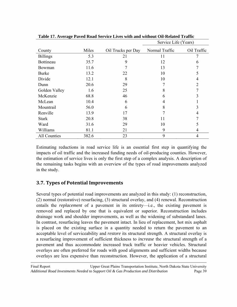
Final Report Upper Great Plains Transportation Institute, North Dakota State University Additional Road Investments Needed to Support Oil & Gas Production and Distribution Page 39
Table 17. Average Paved Road Service Lives with and without Oil-Related Traffic Service Life (Years)
County Miles Oil Trucks per Day Normal Traffic Oil Traffic Billings 5.3 21 11 7 Bottineau 35.7 9 12 6 Bowman 11.6 7 13 7 Burke 13.2 22 10 5 Divide 12.1 8 10 4 Dunn 20.6 29 7 2 Golden Valley 1.6 25 8 7 McKenzie 68.8 46 6 3 McLean 10.4 6 4 1 Mountrail 56.0 6 8 3 Renville 13.9 17 7 4 Stark 20.8 38 11 7 Ward 31.6 29 10 5 Williams 81.1 21 9 4 All Counties 382.6 23 9 4
Estimating reductions in road service life is an essential first step in quantifying the impacts of oil traffic and the increased funding needs of oil-producing counties. However, the estimation of service lives is only the first step of a complex analysis. A description of the remaining tasks begins with an overview of the types of road improvements analyzed in the study.
3.7. TypesofPotentialImprovements
Several types of potential road improvements are analyzed in this study: (1) reconstruction, (2) normal (restorative) resurfacing, (3) structural overlay, and (4) renewal. Reconstruction entails the replacement of a pavement in its entirety—i.e., the existing pavement is removed and replaced by one that is equivalent or superior. Reconstruction includes drainage work and shoulder improvements, as well as the widening of substandard lanes. In contrast, resurfacing leaves the pavement intact. In lieu of replacement, hot mix asphalt is placed on the existing surface in a quantity needed to return the pavement to an acceptable level of serviceability and restore its structural strength. A structural overlay is a resurfacing improvement of sufficient thickness to increase the structural strength of a pavement and thus accommodate increased truck traffic or heavier vehicles. Structural overlays are often preferred for roads with good alignments and sufficient widths because overlays are less expensive than reconstruction. However, the application of a structural

Final Report Upper Great Plains Transportation Institute, North Dakota State University Additional Road Investments Needed to Support Oil & Gas Production and Distribution Page 40
overlay is only cost-effective when the road is resurfaced in a timely manner and the existing base isn’t degraded. Once a road is badly deteriorated and its base is fouled, it cannot be effectively resurfaced.
Normal or restorative resurfacing is the primary improvement envisioned for non-impacted roadways. Without extensive truck traffic, a relatively thin overlay (e.g., 2.25 inches) can be effectively applied.
3.7.1. Reconstruction A road may be reconstructed for several reasons. (1) The pavement is too deteriorated to resurface. Roads in the poor and very poor classifications fall into this group. (2) The road has a degraded base that will provide little structural contribution to a resurfaced pavement. (3) The roadbed is comprised of poor soils that are susceptible to moisture. In this case, reconstruction is necessary to provide year-round service at the maximum legal weight. (4) The road is too narrow to accommodate thick overlays without widening. In this case, reconstruction may be the only alternative that does not reduce capacity or potentially affect safety.
At a minimum, reconstruction will prevent the loss of width. It may also provide for minor widening, shoulder and drainage improvements. As a result, reconstruction may enhance capacity (as measured in vehicles per hour) because of wider lanes and shoulders. Shoulder improvements may enhance safety. Last but not least, reconstruction will remove spring load restrictions and allow year-round operation at gross vehicle weights of 80,000 pounds or greater.
3.7.2. StructuralOverlay A structural overlay is a cost-effective solution (as opposed reconstruction) for pavements with substantial but lower increases in traffic. In this type of improvement, a new asphalt layer is placed on top of the existing pavement. The thickness of the layer may vary. However, it may be as thick as five inches.
A structural overlay may remove spring load restrictions and allow year-round operation at the maximum legal weight. However, this result cannot be guaranteed. The outcome depends upon the existing road and its underlying soils. Old aggregate bases in roads that have never been reconstructed may be largely ineffective. Given the depths of the bases reported in the survey (i.e., from 2 to 6 inches) and their low implied coefficients, these bases are unlikely to provide significant structural contributions to a resurfaced pavement.

Final Report Upper Great Plains Transportation Institute, North Dakota State University Additional Road Investments Needed to Support Oil & Gas Production and Distribution Page 41
Moreover, the bases may be degraded and contaminated with fines. In such cases, structural overlays are not guaranteed to remove spring load restrictions.
3.8. ImprovementLogicandCosts
3.8.1. ImprovementSelectionCriteria
In this study, pavements currently in poor or very poor condition are considered too deteriorated to resurface and are reconstructed. Additional segments with higher traffic volumes are considered for reconstruction because of the width and operational concerns mentioned earlier.
Unfortunately, detailed information such as the graded roadway width and structural number are unknown for each impacted segment. Only aggregate values were obtainable. Without knowledge of the widths of individual segments, reconstruction improvements are allocated to segments based on traffic until a modest level of oil traffic is reached (i.e., 20 trucks per day), subject to an overall constraint of 41% of impacted county collector miles. This constraint corresponds to the generalized estimate presented earlier of the proportion of collector miles with insufficient widths (Table 15).30
Reconstruction is expected to provide year-round heavy-hauling capabilities and thus satisfy the criterion mentioned earlier. Moreover, the allocation of reconstruction dollars to roads with higher traffic levels will maximize capacity and ride-quality benefits for all travelers. When baseline traffic is included, the segments selected for reconstruction may experience 40 or more trucks a day and a greater number of automobile travelers.
Roads not selected for reconstruction are eligible for structural overlays until the oil traffic drops to low levels (i.e., 5 trucks per day). At these levels, oil traffic is a relatively small component of the overall non-oil related traffic base. For these lightly-traveled roads, a different approach is used, in which oil trucks are assigned part of the cost of renewing pavements. This approach is discussed next.
3.8.2. Renewal
Many of the impacted segments reflected in Table 6 are projected to have only a few oil-related trucks per day. While these roads are affected, they do not have the additional
30 Because most of the impacted paved roads are county major collectors, this percentage is used instead of the percentage for local county roads or a weighted average of the two.

Final Report Upper Great Plains Transportation Institute, North Dakota State University Additional Road Investments Needed to Support Oil & Gas Production and Distribution Page 42
traffic to justify reconstruction. Nevertheless, a portion of the costs associated with the renewal of these pavements is not reflected in the baseline and should be accounted for.
In this approach, the life of a road is estimated in ESALs. The cost to renew the road or maintain its serviceability is divided by its ESAL life. For example, the average cost to renew a road with an ESAL life of 40,000 by applying a thin overlay that costs $140,000 per mile is $3.50 per ESAL-mile. In this example, the renewal cost is $9.00 per front-haul tractor-semitrailer mile (i.e., $3.50 per ESAL-mile × 2.57 ESALs). Suppose the pavement life is 80,000 ESALs. In this case, the renewal cost is $4.50 per front-haul tractor-semitrailer mile (i.e., $1.75 per ESAL-mile × 2.57 ESALs).
New Structural Number. In renewal, a new surface layer is assumed to be placed on roads with the structural numbers described in Section 3.3. The structural number after renewal is computed as D1 × A1 + D2 × A2 + D3 × A3. In this calculation, D1 and D2 represent the depths of the existing base and surface layers, respectively, while A1 and A2 represent the structural coefficients of these layers. Similarly, D3 and A3 represent the thickness and structural coefficient of the new surface layer, respectively.
Effective Structural Number. Initially, the new surface layer will have a structural coefficient (A3) of 0.44 per inch. However, as described in AASHTO 1993, the effective coefficient may decline to approximately 0.15 when the pavement reaches poor or very poor condition. The expected (median) value of A3 over the life a pavement is 0.34 (e.g., fair condition). As noted earlier, old aggregate bases in roads that have never been reconstructed may be largely ineffective. Given the low implied coefficients from Tables 8 and 9, A2 and A2 are assigned values of 0.07 and 0.20, respectively. With these inputs, the effective mid-life structural number of a renewed road with an old 6-inch aggregate base and an old 5-inch asphalt surface layer (that now serves as a base) is calculated as 6 × 0.07 + 5 × 0.20 + 2.25 × 0.34 = 2.19.
Cost per ESAL-Mile. The costs per ESAL-mile used in this study range from $0.71 to $10.26 with a mean value of $3.46. At the mean, the cost responsibility of a tractor-semitrailer is $8.90 per front-haul mile when the ESALs associated with the empty movement are considered.
3.8.3. ImprovementCostsperMile The reconstruction cost used in this study is $1.25 million per mile.31 This is the same unit cost used by the North Dakota Department of Transportation to estimate the cost of reconstructing two-lane state highways. Because the cost is reflective of state highways
31 North Dakota Department of Transportation work papers.

Final Report Upper Great Plains Transportation Institute, North Dakota State University Additional Road Investments Needed to Support Oil & Gas Production and Distribution Page 43
with 12-foot lanes, counties should be able to build roads that have 12-foot lanes and some shoulders. Modest alignment improvements may also be possible within the reconstruction budget. However, this unit cost will not cover major realignment. According to the Federal Highway Administration, major realignment of a roadway will increase reconstruction cost by 55 percent per mile.32 In comparison, a structural overlay is assumed to cost $300,000 per mile.
3.9. PavedRoadMaintenanceCosts
Thus far, only construction costs have been analyzed. Once improved, the roads must be maintained over time under heavy truck traffic. Therefore, annual maintenance costs must be considered.
A method for estimating changes in paved road maintenance cost is described in Appendix D. On paved roads, maintenance costs include patching, crack sealing, and the periodic application of seal coats. The method used in this study predicts a 52% increase in maintenance costs when traffic increases from low to medium and a 35 percent increase when traffic grows from medium to high. This method predicts costs of $139,492, $212,322, and $287,522 per mile for low-, medium-, and high-traffic roads respectively for the 20-year analysis period. When annualized, the 20-year costs amount to $6,975, $10,616, and $14,376 per mile of paved road per year for low-, medium-, and high-traffic roads, respectively,
There are no guidelines in this case as to what levels of oil traffic constitute low, medium, and high traffic. As noted earlier, trucks used in the oil industries have substantially higher ESAL factors than baseline trucks. Thus, roads with 20 or more oil-linked trips per day are classified as high-traffic roads because of the heavy weights and high ESAL factors of the trucks. Roads with less than 20 but at least five oil-linked trips a day are classified as medium-traffic roads. These roads also have other (non-oil) traffic that contributes to their classification. Nevertheless, it is assumed that the growth in oil traffic is the driving force behind the classification change.
For a road classified as medium traffic, the additional maintenance cost attributable to oil-related traffic is estimated by subtracting the low-traffic cost of $139,492 per mile from the medium-traffic cost of $212,322 per mile. Similarly, for a road classified as high traffic,
32 In the Highway Economic Requirements System, the indexed 2009 cost for pavement reconstruction of a major collector highway is $1.086 million per mile. In comparison, the cost of pavement reconstruction with realignment is $1.688 million per mile, roughly a 55% increase. The FHWA’s unit costs are not as specific or current as the ones provided by the North Dakota Department of Transportation. Therefore, they are not used in this study.

Final Report Upper Great Plains Transportation Institute, North Dakota State University Additional Road Investments Needed to Support Oil & Gas Production and Distribution Page 44
the additional maintenance cost attributable to oil-linked traffic is estimated by subtracting the low-traffic cost of $139,492 per mile from the high-traffic cost of $287,522 per mile.
To put these numbers in perspective, the annualized cost of two seal coats applied during a 20-year service life is equal to $2,800 to $3,500 per mile per year.33 In a medium-traffic scenario, a county would have approximately $7,100 to $7,800 per mile per year to spend on other activities, such as crack sealing and patching of impacted roads. In a high-traffic scenario, the county would have $10,900 to $11,600 per mile per year for crack sealing and patching.
Note that the annualized costs reflect all traffic on the roadways: oil-related, baseline truck, and automobile. The predicted increase in annual maintenance cost attributable to moving from a low- to a medium-traffic category is $3,641 per mile. The predicted increase in annual maintenance cost attributable to moving from a low- to a high-traffic category is $7,400 per mile. These are the additional costs due to growth in oil traffic. The remainder is baseline cost.
The costs presented in this section of the report are theoretical estimates based on little experience about the actual maintenance effects of oil-related traffic. At present, none of the counties have the resources to spend $6,975 per mile per year on the maintenance of paved roads. This issue will be discussed in the conclusion.
3.10. EstimatedPavedRoadFundingNeeds
The results of the paved road analysis are presented in several ways. First, the results are presented by biennium. Next, the results are summarized by improvement type. Third, the results are summarized by county. In each case, the funding needs associated with oil growth are compared to the theoretical baseline funding needs. However, several interpretive cautions must be noted.
The baseline costs reflect only direct roadway costs. Administrative and other overhead costs are not included. To gain a truer picture of the baseline cost, county expenses would have to be allocated to the miles of impacted road. This could be a complicated process because county personnel serve many roles and deal with many issues other than transportation. Suffice it say that baseline costs are understated because they do not include administrative and co-related costs. Furthermore, baseline costs are for all paved roads in impacted counties.
33 Two cost estimates of seal coats were obtained during this study. The higher estimate of $35,000 per mile is applicable to Federal-Aid highways. The lower cost is $28,000 per mile.

Final Report Upper Great Plains Transportation Institute, North Dakota State University Additional Road Investments Needed to Support Oil & Gas Production and Distribution Page 45
3.10.1. FundingNeedsbyTimePeriod
Column 2 of Table 18 shows the oil-related funding needs. These are additional needs on paved county roadways which can be directly attributed to oil development in western North Dakota.
Table 18. Estimated Additional Paved Road Funding Needs by Period ($ 2010)*
Costs in Millions of Dollars Period Oil Related Needs
2012-2013 $118.0 2014-2015 $149.8 2016-2017 $16.8 2018-2019 $20.5 2020-2021 $10.4 2022-2023 $6.1 2024-2025 $4.7 2026-2027 $4.2 2028-2029 $4.2 2030-2031 $4.2 All Periods $338.9
* Excludes costs of special vehicles, overhead expenditures
As the table shows, the estimated oil-related costs amount to $338.9 million over the 20-year period. These costs are a function of projected increases of oil production and distribution and the predicted remaining lives of pavements. Most of the funds ($229.2) will be needed during the next two biennia as impacted roads become candidates for improvement. When annualized, these costs amount to roughly $17 million per year of additional roadway investment needs as a result of oil growth.34
3.10.2. FundingNeedsbyImprovementType Funding needs by improvement type are shown in Table 19. These improvements relate to the oil-impacted paved road segments. Of the extimated costs, 76% are attributable to reconstruction. Sixty-eight of these miles consist of roads that are currently in poor or very
34 Detailed information regarding the bases and underlying soils of impacted segments could improve the reliability of the estimates. However, this information would require months of additional field work to acquire samples of base and soil materials beneath the impacted segments or to determine the underlying support via deflection testing.

Final Report Upper Great Plains Transportation Institute, North Dakota State University Additional Road Investments Needed to Support Oil & Gas Production and Distribution Page 46
poor condition. The remainder includes higher traffic roads selected because of the benefits that will result from eliminating width constraints and spring load restrictions.35 Approximately 12% of the costs are attributable to structural overlays of less traveled oil routes. It should be noted that the maintenance cost estimates assume that the reconstruction and overlay improvements are implemented. If reconstruction and overlay improvements on deteriorated pavements are not made or postponed, the corresponding maintenance activities and associated costs will increase.
Table 19. Estimated Additional Paved Road Funding Needs by Improvement Type ($ 2010)*
Type Costs in Millions of Dollars Miles Oil Related Needs
Maintenance 958.4 $41.6 Overlay 249.4 $39.8
Reconstruction 225.6 $256.1 Renewal 483.4 $1.3 All Types . $338.9
* Excludes costs of special vehicles, overhead expenditures
3.10.3. FundingNeedsbyCounty
The estimated costs by county are shown in Table 20. This distribution reflects several factors: (1) the miles and proportions of paved roads in various counties, (2) originated and/or terminated oil-related traffic, (3) through oil traffic, and (4) the conditions and structural capacities of paved roads.
3.10.4. EffectsofInvestments Reconstruction. Approximately 256 miles of county road were selected for possible reconstruction.36 These roads are some of the most heavily impacted oil routes. Moreover,
35 In total, 48 percent of the miles selected for reconstruction or overlay are reconstructed in the analysis. This percentage includes 68 miles of road reconstructed because of poor or very poor condition. After subtracting out those miles, 39 percent of the miles selected for reconstruction or overlay are reconstructed. This is less than the constraint of 41 percent because the number of miles with 20 or more oil trucks per day are exhausted before the constraint is reached. 36 The actual allocation of miles of road with insufficient widths is unknown. Some of the individual road segments selected for reconstruction may have sufficient widths. If so, the justifications for reconstruction may be weakened. However, some of the roads selected for structural overlays may prove to have insufficient widths and, therefore, must eventually be reconstructed. In totality, the miles selected for reconstruction may shift

Final Report Upper Great Plains Transportation Institute, North Dakota State University Additional Road Investments Needed to Support Oil & Gas Production and Distribution Page 47
they have some of the highest baseline truck and automobile traffic volumes. The reconstruction investments will eliminate spring load restrictions while providing paved roads that should last 18 to 20 years in the face of escalating heavy truck traffic. The reconstructed and widened roads will enhance safety as a result of 12-foot lanes and shoulders. Moreover, the wider roads will reduce the interference of traffic moving in opposite directions and increase roadway capacity. Last but not least, the newly reconstructed roads will improve ride quality for all users. Structural Overlay. An additional 249 miles of paved road are candidates for structural overlays. These roads have lower projected estimates of oil-linked traffic than the roads selected for reconstruction. However, without thicker overlays, their life expectancies will be significantly reduced from baseline levels.37 A structural overlay may mitigate or lessen the severity of a spring restriction—e.g., exchange a 6-ton restriction for a less severe one. In some cases, the increased structural number from the overlay may allow 80,000-pound gross vehicle weights year round. However, these outcomes are very site-specific and dependent upon the quality of the underlying soil. At a minimum, a thick overlay should provide for an 18-to-20-year service life with moderate oil-related traffic. Pavement Renewal. The renewal costs estimated for lightly-traveled routes with less than five predicted oil trucks per day should compensate for additional damage and help maintain an 18-to-20-year service life. Annual Maintenance. The annual maintenance funds should provide sufficient resources to preserve the capital investments in reconstructed and widened roadways and segments that are upgraded through structural overlays. Maintenance activities include two optimally-timed seal coats, crack sealing, patching, striping, etc. However, the projected maintenance costs do not reflect increased snow removal activities on oil routes. As mentioned above, the maintenance estimates assume that the reconstruction and overlay improvements are implemented.
3.11. ImpactsofSpecialVehicles
The effects of specialized vehicles have yet to be considered. Movements of rig equipment, fracturing equipment, utility vehicles, workover rigs and other drilling related equipment
among the high and moderate oil-traffic groups. However, the overall number of miles reconstructed should be roughly the same. 37 The cost per inch of asphalt surface is approximately $60,000. At a cost of $300,000 per mile, a five-inch overlay could be applied to an impacted road. Initially, a five-inch overlay would increase the structural number of the road by 2.2; which is a healthy increase. Over time, the structural contribution of the new surface layer would drop with the growth of distresses such as alligator cracking.

Final Report Upper Great Plains Transportation Institute, North Dakota State University Additional Road Investments Needed to Support Oil & Gas Production and Distribution Page 48
and vehicles are difficult to model. A set of origins and destinations for oil, sand, water and other movements can be predicted with some accuracy. However, special vehicles move in irregular routes from one drilling location to another. This analysis assumes that the movements are in accordance with the regulations listed in the North Dakota Highway Patrol Permit Policy for Movement of Oversize and Overweight Vehicles and/or Loads. Table 20. Estimated Additional Paved Road Funding Needs by County ($ 2010)*
County Costs in Millions of Dollars
Oil Related Needs Billings $3.4
Bottineau $9.1 Bowman $2.7
Burke $8.9 Divide $6.7 Dunn $24.2
Golden Valley $3.5 McHenry $0.0 McKenzie $63.3 McLean $13.0 Mercer $0.0
Mountrail $76.0 Renville $22.8
Slope $0.0 Stark $31.9 Ward $21.2
Williams $52.2 All Counties $338.9
* Excludes costs of special vehicles, overhead expenditures
The number of impacted paved segments has been estimated through 2013. These estimates are 47 miles in 2011, 79 miles in 2012, and 68 miles in 2013. These distances have been extrapolated to 2022, when production is estimated to be the dominant traffic generator. Moreover, ESAL factors have been estimated for each type of vehicle. The average ESAL factor is 8.36 per vehicle, or 418.42 ESALS for all 50 vehicles. The mean cost per ESAL for county roads ($3.46) is used to estimate the total effect. Because the specific routes of these vehicles cannot be accurately projected, the costs cannot be assigned to counties with certainty. However, the costs can be accumulated by

Final Report Upper Great Plains Transportation Institute, North Dakota State University Additional Road Investments Needed to Support Oil & Gas Production and Distribution Page 49
time period. The total estimated cost from 2011 through 2022 is $1.21 million. The projected costs are $182,545 in fiscal year 2012-2013, $280,267 for fiscal years 2014-2016, $446,191 for fiscal years 2017-2021, and $212,064 in fiscal year 2022-2023. These special-vehicle costs are added to the costs from Table 18 to produce Table 21, which shows all paved road costs by period.
Table 21. Total Estimated Additional Paved Road Funding Needs by Period ($ 2010 Million)*
Period Oil Traffic 2012-2013 $229.3
2014-2016 $41.0
2017-2021 $44.5
2022-2026 $14.7 2027-2031 $10.5 All Periods $340.0
*Not including overhead expenditures
Only the paved road funding needs are presented in Tables 18-21. The report now turns to the topic of unpaved road impacts and funding needs. The discussion begins with an overview of the types of roads being analyzed and a synopsis of the analysis methods.

Final Report Upper Great Plains Transportation Institute, North Dakota State University Additional Road Investments Needed to Support Oil & Gas Production and Distribution Page 50
4. UnpavedRoadAnalysis
The unpaved roads analyzed in this study include two primary categories: Gravel and Graded & Drained. The gravel roads represent county maintained infrastructure, and the Graded & Drained roads represent township infrastructure. Each road type is classified by the impacted traffic level: Low, Elevated, Moderate, or High. The methods used to analyze unpaved roads are discussed next.
4.1. Methodology
The life-cycle costs of a road include the initial improvement cost and expected annual maintenance costs. For every type of road surface, maintenance costs increase with increases in traffic. However, the amount of the increase attributable to increased traffic varies by surface type. Additionally, the improvement cost varies greatly depending on the surface type. On gravel surfaces, as the ADT increases, the frequency of blading and gravel application must increase to preserve surface quality. For paved surfaces, the additional maintenance is less than for gravel sections. However, the initial improvement cost is higher for paved roads. There exists a threshold where the total life-cycle cost for a paved surface is less than for gravel surfaces. Table 22 outlines the relative initial improvement costs for gravel and double chip seal under different gravel application cycles. This example assumes a $30,000 per mile gravel overlay cost and $200,000 for a double chip seal application including grading and widening. Both costs in this example exclude maintenance. As shown in the table, a typical five year gravel cycle results in a $60,000 improvement cost over 10 years. If the traffic on this example mile increases, it may be necessary to shorten the cycle length and apply a gravel overlay more frequently. In this scenario, if gravel is applied more than every 2 years on average, the chip seal surface becomes the more cost-effective improvement type. Table 22: Life-Cycle Cost Comparisons Between Gravel and Chip Seal Surfaces
Gravel Cycle Gravel Cost/10 years Double Chip Seal Cost/10 years
5 year $60,000 $200,000
4 year $70,000 $200,000
3 year $100,000 $200,000
2 year $150,000 $200,000
1 year $300,000 $200,000

Final Report Upper Great Plains Transportation Institute, North Dakota State University Additional Road Investments Needed to Support Oil & Gas Production and Distribution Page 51
The South Dakota Department of Transportation compiled costs for different surface types, and compared the cost levels for gravel, blotter and hot mix asphalt at different traffic levels.38 The report indicates that at a traffic level of 150 vehicles per day a paved surface (double chip seal) has a lower life-cycle cost than a gravel surface. The Minnesota Department of Transportation39 indicates that life-cycle costs are equal for gravel and chip seal surfaces between 150 and 199 ADT. Due to the high truck percentage of traffic on impacted roads, it is assumed that the lower threshold is applicable. Since the publication of these studies, county road departments have experienced inflation in construction cost components. The cost components were indexed for inflation using the construction cost index from the North Dakota Department of Transportation, and the ADT thresholds outlined in the documents were found to be valid.
4.1.1. Classification
The unpaved sections are classified by the estimated additional truck traffic due to increased oil development. The categories include: (1) low (0-25), (2) elevated (25-50), moderate (50-100), and high (100+). The baseline traffic for graded & drained roads and gravel roads is 15 and 50 respectively. Estimates from a 2007 survey of county road officials indicate that these assumptions are sound for baseline traffic. The non-oil related traffic level is essential to calculating the total impacts, as the total traffic; baseline plus oil-related traffic, determines whether the paving threshold has been met.
4.1.2. ImprovementTypes
Graded & Drained. Three improvement types are modeled for graded & drained roads: no improvement, increase gravel application, or upgrade to gravel structure. For the low-impact category, it is assumed that little additional work will be done to the road surface. For the elevated impact category, the improvement is to shorten the gravel application cycle by 50%. For the moderate and high impact categories, the selected improvement is upgrading the roadway to a gravel surface. Since the initial condition of graded and drained roads are often deficient with respect to roadway width, the upgrade involves regrading of the road, and addition of width to a minimum of 24 feet, and the gravel overlay.
Gravel. Four improvement types are modeled for gravel roads: decreasing the blading interval, decreasing the gravel interval by 33%, decreasing the gravel interval by 50% and
38 Local Road Surfacing Criteria, South Dakota Department of Transportation, Study SD2002-10, June 2004. 39 Economics of Upgrading an Aggregate Road, Minnesota Department of Transportation, MN/RC 2005-09, January 2005

Final Report Upper Great Plains Transportation Institute, North Dakota State University Additional Road Investments Needed to Support Oil & Gas Production and Distribution Page 52
the application of a double chip seal to conserve and preserve aggregate4041. The double chip seal treatment has been successfully implemented in parts of the state for this purpose, but at present is not implemented statewide. As mentioned above, when traffic approaches 150 ADT and when a high percentage of trucks are present, the chip seal treatment becomes the lower cost option when life-cycle cost is considered. Using that rationale, the high impact category meets this threshold and receives the double chip seal treatment.
Survey questions asked the county officials to provide the gravel and blading cycles for non-impacted gravel roads and impacted gravel roads. The consensus from the survey responses was that on impacted roads, the gravel interval decreases and the number of bladings per month increase. For example, a non-impacted road has a gravel cycle of 5 years and a blade interval of once per month, while an impacted section has a gravel cycle of 2 to 3 years and a blade interval of twice per month. The effective difference is a doubling of the gravel maintenance costs over the same time period. On the low impact road sections, increased blading activity is implemented to maintain roadway surface condition.
In addition to the increases in routine maintenance on the elevated and moderate impact gravel road sections, dust suppressant and road reconstruction improvements have been identified. Currently, in the heavily impacted counties, dust suppressant is used to preserve surface aggregate and to mitigate the dust related safety and health impacts. Estimates of the number of miles of currently impacted roads receiving dust treatment are consistent with reports from heavily impacted counties. The estimates for the elevated and moderate impact categories also reflect reconstruction during the first period to repair road deficiencies. These deficiencies include roadway width and structural deficiencies which, when corrected allow for 12 month operation.
For purposes of this analysis, all graveling intervals were converted to a base five-year interval. That is, if a county reported a one-year gravel interval, the costs were converted to a five-year total graveling cost.
40 E. Horak, et al, Risk Managed Design Standards for Upgrading of Basic Access Gravel Streets, Proceedings of the 8th Conference on Asphalt Pavements for Southern Africa, September 2004.
41 C. Overby and M.I. Pinard, Appropriate Standards and Specifications for Surfacing of Low-Volume Rural Roads, 12th International Conference of the International Association for Computer Methods and Advances in Geomechanics, October 2008

Final Report Upper Great Plains Transportation Institute, North Dakota State University Additional Road Investments Needed to Support Oil & Gas Production and Distribution Page 53
4.2. ResultsforUnpavedRoads
Approximately 12,718 miles of impacted unpaved roads have been identified (Table 23). According to the surveys, 37% of these miles are in good or very good condition. Another 58% are in fair condition. Five percent of these miles are in poor or very poor condition (Table 24).
4.2.1. UnpavedRoadCostsbyCounty
The unpaved road needs are shown for each county in Table 25. This distribution reflects several factors: (1) the miles and proportions of roads in various counties, (2) originated and/or terminated oil-related traffic, and (3) through oil traffic. Note that these costs do not include overhead expenditures, rather component and maintenance costs specifically.
4.2.2. UnpavedRoadCostsbyTimePeriod
The projected costs by time period are shown in Table 26. The projected improvements for unpaved roads are shown by county and road type (e.g., graveled versus graded and drained) in Appendix D.

Final Report Upper Great Plains Transportation Institute, North Dakota State University Additional Road Investments Needed to Support Oil & Gas Production and Distribution Page 54
Table 23. Miles of Unpaved Road Impacted by Oil-Related Traffic County Gravel* Graded & Drained
Billings 560 28 Bottineau 924 113 Bowman 230 42 Burke 912 106 Divide 1,076 63 Dunn 968 105 Golden Valley 413 40 McHenry 335 24 McKenzie 1,046 69 McLean 451 34 Mercer 36 1 Mountrail 1,294 71 Renville 677 21 Slope 97 5 Stark 737 48 Ward 633 48 Williams 1,444 65 Total 11,834 884 *Gravel miles include a portion of township roads
Table 24. Reported Conditions of Impacted Unpaved Roads
Road Condition Miles Percent Miles Cumulative
Miles Cumulative
Percent Very Good 118.2 0.9% 118.2 0.9% Good 4,601.9 36.18% 4,720.1 37.1% Fair 7,374.2 57.98% 12,094.3 95.1% Poor 574.3 4.52% 12,668.6 99.6% Very Poor 49.3 0.4% 12,717.9 100%

Final Report Upper Great Plains Transportation Institute, North Dakota State University Additional Road Investments Needed to Support Oil & Gas Production and Distribution Page 55
Table 25. Projected Additional Unpaved Needs by County ($ 2010 Million)
Gravel Graded & Drained County Oil Related Needs Oil Related Needs
Billings $18.30 $0.30 Bottineau $6.60 $0.00 Bowman $2.10 $0.00 Burke $17.10 $0.80 Divide $47.90 $0.40 Dunn $75.60 $5.40 Golden Valley
$22.70 $0.30
McHenry $3.30 $0.10 McKenzie $81.70 $4.40 McLean $21.10 $1.10 Mercer $0.80 $0.00 Mountrail $76.10 $0.90 Renville $11.10 $0.60 Slope $2.50 $0.30 Stark $35.70 $0.90 Ward $29.30 $0.70 Williams $97.20 $1.90
Total $548.90 $18.10
Table 26. Projected Additional Oil Related Unpaved Road Needs by Time Period ($ 2010 Million)* Time Period Oil Related Cost 2012-2013 $114.9 2014-2016 $172.3 2017-2021 $92.2 2022-2026 $122.8 2027-2031 $64.9 Total $567.0
*Excludes overhead expenditures

Final Report Upper Great Plains Transportation Institute, North Dakota State University Additional Road Investments Needed to Support Oil & Gas Production and Distribution Page 56
5. SensitivityAnalysis
The analysis is based on models and detailed data where possible. Nevertheless, some key assumptions were made during the study; in particular, assumptions regarding threshold traffic levels that trigger reconstruction or changes in maintenance costs. The effects of those thresholds are evaluated in this section of the report.
5.1. ReconstructionofPavedRoads
Approximately 226 miles of impacted paved roads were selected for reconstruction in the analysis. Only those roads with the highest oil-related traffic volumes were selected. A threshold of 20 oil-related trucks per day was used. As noted earlier, with 20 additional trucks per day, a paved road may have 100 ADT when baseline trucks and other vehicles are considered.
Some may argue 20 oil-related trucks per day with 100 ADT is a liberal threshold for reconstruction. However, the trucks used by the oil industries have much higher ESAL factors than baseline trucks. The average impact factor of specialized vehicles is 8.36 ESALs per mile. The average impact factor of other oil-related trucks is 2.57 ESALs per front-haul mile. Further, there are justifications for reconstruction other than added structural strength. The reconstructed segments will have wider lanes and shoulders. Moreover, year-round operations will be possible. Consequently, reconstruction will offer safety and capacity benefits as well as improved structural strength. Nevertheless, it is important to analyze other alternatives and the sensitivities of the conclusions to alternative assumptions. Two sensitivity scenarios are analyzed. In the first scenario, the oil traffic threshold for reconstruction is raised to 40 trucks per day. With 40 additional trucks per day, a paved road may be approaching 200 ADT when baseline trucks and other vehicles are considered. Using this threshold reduces the number of miles selected for reconstruction from 226 to 169. As a result, the predicted funding need (Table 21) drops from $340 million to $284 million. In the second scenario, the oil traffic threshold for reconstruction is raised to 100 trucks per day. With 100 additional oil trucks per day, a paved road may be approaching 500 ADT when baseline trucks and other vehicles are considered. Using this threshold reduces the number of miles selected for reconstructed from 226 to 147. As a result, the predicted funding need drops from $340 million to $263 million.

Final Report Upper Great Plains Transportation Institute, North Dakota State University Additional Road Investments Needed to Support Oil & Gas Production and Distribution Page 57
5.2. PavedRoadMaintenance
Approximately $41.6 million of oil-ascribed maintenance costs were predicted for the 20-year period for the 958 miles of impacted paved road (Table 19). This amounts to an average of $2,171 per mile per year.
In the analysis, it was assumed that as few as five oil-related trucks per day could change a road’s maintenance classification from low to medium. The primary justification for such a low threshold was voiced during the fact-finding meetings conducted by the Department of Commerce. During the fact-finding tour, county managers asserted that only a few oil trucks or specialized vehicles per day could greatly increase road maintenance cost because of their heavy gross weights and high ESAL factors. The heavy gross weights cause rutting, while the high ESAL factors accelerate cracking and lead to more frequent crack sealing, patching, and spot maintenance.
With little historical data regarding the maintenance effects of oil trucks and specialized vehicles, strong weight was given to the anecdotal assessments of county road managers. For similar reasons, a threshold of 20 oil-related trucks per day was used to define high maintenance roads.
Some may argue these thresholds are liberal. Therefore, sensitivity analysis is performed to assess their effects. In sensitivity analysis, a medium maintenance road is defined as one with at least 20 (but less than 40) oil-related trucks per days. A high maintenance road is defined as one with 40 or more oil-related trucks per days. These changes reduce the annual oil-related maintenance cost to less than $1,000 per year per mile of impacted road. As a result, the predicted investment needs drop from $340 million to $260 million.
5.3. ReconstructionofUnpavedRoads
Approximately 1,420 miles of county gravel roads were reconstructed in this analysis. The rationale for this reconstruction is to correct any problems such as subgrade deficiencies or roadway width. These improvements would improve safety and allow for year round operation over impacted segments. In the analysis, the elevated and moderately impacted road segments are selected for this improvement. These sections represent 25-50 and 50-100 additional truck ADT due to increased oil development. Using a cost of $100,000 per mile, the reconstruction improvements total $142.1 million. In the analysis, most roads are estimated to be reconstructed during the first five years of the analysis period.
Due to the increased traffic, increased gravel application and maintenance would occur whether or not the roadway would be reconstructed. This reflects current practices that were reported in the county survey responses. The underlying assumption is when

Final Report Upper Great Plains Transportation Institute, North Dakota State University Additional Road Investments Needed to Support Oil & Gas Production and Distribution Page 58
additional traffic exceeds 25 ADT roadway damage would be significant during wet periods or during the spring thaw period (Figure 3). If this threshold is raised to 50 additional ADT, the reconstruction cost would decrease to $38.5 million, and the total cost to $528 million. If reconstruction were limited to upgrade of graded and drained roads and upgrades to double chip seal, the total cost would be $424.8 million.
6. OverheadExpenditures
6.1. OverheadExpenditures
As noted in the results section for both paved and unpaved roadways, the baseline estimates do not include overhead expenditures. The estimates reflect the direct costs of the road improvements. For this reason, the baseline estimates should not be used to represent total county road maintenance budgets. Informal estimates of the level of overhead range from 35% to 50% percent of the direct road maintenance activities. The overhead expenditures were omitted from the cost estimates for a number of reasons. The heterogeneity of county road departments is the underlying issue. Depending on the county, the level of services that are provided internally varies significantly. For example, one county may have an engineer on staff, while the next must contract with an outside engineering firm for services. Wage rates vary from county to county, and due to competition from oil development companies for labor, these wage rates may fluctuate significantly. Additionally, county shop facilities vary from county to county. Moreover, as county roadway departments grow larger, additional labor and infrastructure may be needed, and it is unlikely that the existing level of overhead expenditures as a percentage of direct road expenditures will increase proportionally.
7. ImpactsofInflation
Significant increases in the cost of components for road improvements have occurred over the past 10 years. These increases can be attributed to increases in petroleum prices and the impacts on production of components. Two inflation scenarios have been constructed, representing a low and moderate inflation rate continued throughout the study timeframe. The scenarios are 3 and 5 percent inflation. Both scenarios assume that the level of inflation would remain constant

Final Report Upper Great Plains Transportation Institute, North Dakota State University Additional Road Investments Needed to Support Oil & Gas Production and Distribution Page 59
throughout the 20-year timeframe, and are designed as an illustration of the impacts on inflation on roadway needs. Recall that in 2010 dollars, the total oil-related need was $907 million during the next 20 years. Also, a large proportion of the estimated needs occur in the first five years of the analysis period. Under the 3% scenario, the total estimated 20 year oil-related need is $1,099 million. Under the 5% inflation scenario, the total estimated 20 year oil-related need is $1,266 million.
8. Conclusion
The purpose of this study is to forecast oil-related road investment needs in the oil producing counties of North Dakota over the next 20 years. The essential objective is to quantify the additional investments necessary for efficient year-round transportation of oil while providing travelers with acceptable roadway service. The focus is on roads owned or maintained by local governments. The bottom-line estimates from the study are:
A projected additional investment need of $567 million for unpaved roads during the next 20 years (from 2011 through 2030)
A projected additional investment need of $340 million for paved roads during the next 20 years
A total additional investment need of $907 million during the next 20 years An average annual additional need of $45.35 million over the 2011-2030 period
The short time frame limited the analysis that could be undertaken in this study.42 Some important issues were undoubtedly missed. One such issue is the potential need for rail-highway grade crossing improvements in light of the increased truck traffic on many routes. The North Dakota Department of Transportation has identified 411 passive at-grade railroad crossings on branch lines and mainlines in oil-producing counties that are potential candidates for some type of improvement or closure (Table 27). Potential improvements could include signalization, surface upgrades, road approach work, or signage. Obviously, all of the 411 crossings do not need to be improved because of oil traffic. Nevertheless, a certain number of them are candidates for improvement primarily because of oil-related traffic.
42 The signed contract from Department of Commerce which allowed full-time work to commence on the project was received on August 9. Essentially, the study was conducted in four months. This precluded a lot of detailed field investigations with the exception of the traffic counts.

Final Report Upper Great Plains Transportation Institute, North Dakota State University Additional Road Investments Needed to Support Oil & Gas Production and Distribution Page 60
Table 27. Passive Rail-Highway Grade Crossings that may be Potential Candidates for Improvement
Number of Crossings Location 46 BNSF Mainline Berthold to Montana State Line 24 BNSF Mainline Dickinson to Montana State Line 18 BNSF Mainline East Bowman County Line to Montana State Line 64 CP Rail Mainline Carpio to Canadian Line
152 Total Potential Mainline Crossings 8 Yellowstone Valley Branch line
25 BNSF Powers Lake Branch line 75 DMVW Branch line Flaxton to Montana State Line 75 CP Rail Max to Newtown Branch line 19 BNSF Niobe to Canadian Branch line 57 BNSF Berthold to Lignite Branch-line
259 Total Potential Branch-line Crossings

Final Report Upper Great Plains Transportation Institute, North Dakota State University Additional Road Investments Needed to Support Oil & Gas Production and Distribution Page 61
9. AppendixARoadConditionSurveyandRatingInstructions
County Road Oil Development Impact Study – Map Instructions and Pavement Condition Guide for County Paved Roads
Condition Code
Pavement Condition
Pavement Description
1 Very Good
Only new (or nearly new) superior pavements are likely to be smooth enough and distress free (sufficiently free of cracks and patches) to qualify for this category. Most pavements constructed or resurfaced during the past year would normally be rated in this category.
2 Good
Pavements in this category, although not quite as smooth as those described above, give a first class ride and exhibit few, if any, visible signs of surface deterioration. Pavements may be beginning to show evidence of rutting and fine random cracks.
3 Fair
The riding qualities of pavements in this category are noticeably inferior to those of new pavements, and may be barely tolerable for high-speed traffic. Surface defects of pavements may include rutting, map cracking, and extensive patching.
4 Poor
Pavements in this category have deteriorated to such an extent that they affect the speed of free-flow traffic. Pavements may have large potholes and deep cracks. Distress includes raveling, cracking, rutting and occurs over 50 percent of the surface.
5 Very Poor
Pavements in this category are in extremely deteriorated condition. The road is passable only at reduced speeds, and with considerable ride discomfort. Large potholes and deep cracks exist, and distress occurs over 75 percent or more of the surface.
Adapted from the Highway Performance Monitoring System (HPMS) Field Manual Table IV-4. Please use the enclosed marker to highlight the roads in your county that are paved. Please report the pavement condition on the county map. The pavement conditions, as
listed in the table, are 1) Very Good, 2) Good, 3) Fair, 4) Poor, and 5) Very Poor. Please write the condition code (1-5) by each roadway. If there are segments of a particular road with differing conditions, draw a line through the roadway and note that there is a change in condition. See the attached map for an example.
For Very Good pavements write “1” on the map alongside the road section. For Good pavements write “2” on the map alongside the road section. For Fair pavements write “3” on the map alongside the road section. For Poor pavements write “4” on the map alongside the road section. For Very Poor pavements write “5” on the map alongside the road section.

Final Report Upper Great Plains Transportation Institute, North Dakota State University Additional Road Investments Needed to Support Oil & Gas Production and Distribution Page 62
Pavement Condition Guide for County Gravel Roads
Condition Code
Road Condition Gravel Road Description
1 Very Good No distress, dust controlled, excellent surface condition and ride.
2 Good Dust under dry conditions, moderate loose aggregate, slight washboarding.
3 Fair
Good crown, gravel layer is adequate, but additional aggregate is necessary in isolated areas, moderate washboarding over 10-25% of the area, moderate dust – partial obstruction of vision, none or slight rutting, some loose aggregate.
4 Poor
Little or no crown, some areas with little or no aggregate, moderate to severe washboarding, moderate rutting over 10-25% of the area, moderate potholes over 10-25% of the area, severe loose aggregate
5 Failed
No roadway crown, or road is bowl-shaped, severe rutting (>3 inches deep) over at least 25% of the area, severe potholes (over 4 inches deep) over at least 25% of the area, many areas with little or no aggregate
Please report the pavement condition on the county map. The gravel road conditions, as
listed in the table, are 1) Very Good, 2) Good, 3) Fair, 4) Poor, and 5) Failed. Please write the condition code (1-5) by each gravel roadway. If there are segments of a particular road with differing conditions, draw a line through the roadway and note that there is a change in condition. See the attached map for an example.
For Very Good gravel sections write “1” on the map alongside the road section. For Good gravel sections write “2” on the map alongside the road section. For Fair gravel sections write “3” on the map alongside the road section. For Poor gravel sections write “4” on the map alongside the road section. For Very Poor gravel sections write “5” on the map alongside the road section.
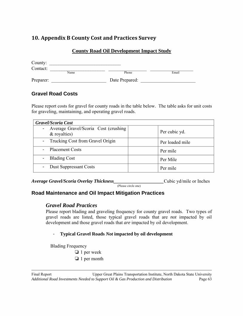
Final Report Upper Great Plains Transportation Institute, North Dakota State University Additional Road Investments Needed to Support Oil & Gas Production and Distribution Page 63
10. AppendixBCountyCostandPracticesSurvey
County Road Oil Development Impact Study County: ______________________________ Contact: _______________________ ________________ __________________
Name Phone Email
Preparer: _______________________ Date Prepared: _______________________
Gravel Road Costs Please report costs for gravel for county roads in the table below. The table asks for unit costs for graveling, maintaining, and operating gravel roads.
Gravel/Scoria Cost - Average Gravel/Scoria Cost (crushing
& royalties) Per cubic yd.
- Trucking Cost from Gravel Origin Per loaded mile
- Placement Costs Per mile
- Blading Cost Per Mile
- Dust Suppressant Costs Per mile
Average Gravel/Scoria Overlay Thickness_____________________Cubic yd/mile or Inches (Please circle one)
Road Maintenance and Oil Impact Mitigation Practices
Gravel Road Practices Please report blading and graveling frequency for county gravel roads. Two types of gravel roads are listed, those typical gravel roads that are not impacted by oil development and those gravel roads that are impacted by oil development.
- Typical Gravel Roads Not impacted by oil development
Blading Frequency
❏ 1 per week ❏ 1 per month

Final Report Upper Great Plains Transportation Institute, North Dakota State University Additional Road Investments Needed to Support Oil & Gas Production and Distribution Page 64
❏ 2 per month ❏ other (please explain)
Typical Gravel Roads Not impacted by oil development cont.
Graveling Frequency ❏ Every year ❏ Every 2-3 years ❏ Every 3-4 years ❏ 5 or more years ❏ other (please explain)
- Oil Impacted Gravel Roads
Blading Frequency
❏ 1 per week ❏ 1 per month ❏ 2 per month ❏ other (please explain)
Graveling Frequency
❏ Every year ❏ Every 2-3 years ❏ Every 3-4 years ❏ 5 or more years ❏ other (please explain)
What maintenance practices are being used to mitigate the impacts of oil development
on the county gravel roads? Paved Road Practices
Please report paved road maintenance practices used in response to oil-related traffic.
What maintenance practices are being used to mitigate the impacts of oil-related traffic on the county paved roads until the county can reconstruct or resurface the pavement?
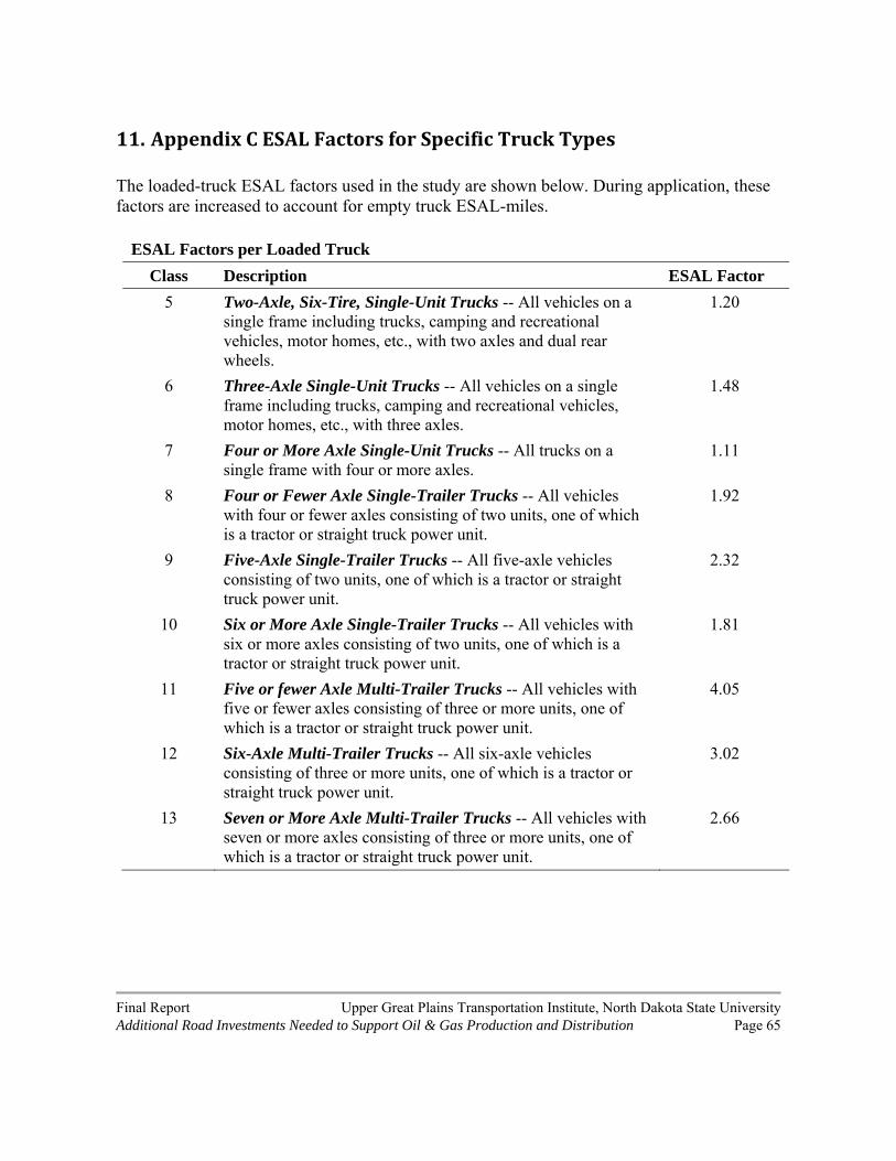
Final Report Upper Great Plains Transportation Institute, North Dakota State University Additional Road Investments Needed to Support Oil & Gas Production and Distribution Page 65
11. AppendixCESALFactorsforSpecificTruckTypes
The loaded-truck ESAL factors used in the study are shown below. During application, these factors are increased to account for empty truck ESAL-miles.
ESAL Factors per Loaded Truck
Class Description ESAL Factor
5 Two-Axle, Six-Tire, Single-Unit Trucks -- All vehicles on a single frame including trucks, camping and recreational vehicles, motor homes, etc., with two axles and dual rear wheels.
1.20
6 Three-Axle Single-Unit Trucks -- All vehicles on a single frame including trucks, camping and recreational vehicles, motor homes, etc., with three axles.
1.48
7 Four or More Axle Single-Unit Trucks -- All trucks on a single frame with four or more axles.
1.11
8 Four or Fewer Axle Single-Trailer Trucks -- All vehicles with four or fewer axles consisting of two units, one of which is a tractor or straight truck power unit.
1.92
9 Five-Axle Single-Trailer Trucks -- All five-axle vehicles consisting of two units, one of which is a tractor or straight truck power unit.
2.32
10 Six or More Axle Single-Trailer Trucks -- All vehicles with six or more axles consisting of two units, one of which is a tractor or straight truck power unit.
1.81
11 Five or fewer Axle Multi-Trailer Trucks -- All vehicles with five or fewer axles consisting of three or more units, one of which is a tractor or straight truck power unit.
4.05
12 Six-Axle Multi-Trailer Trucks -- All six-axle vehicles consisting of three or more units, one of which is a tractor or straight truck power unit.
3.02
13 Seven or More Axle Multi-Trailer Trucks -- All vehicles with seven or more axles consisting of three or more units, one of which is a tractor or straight truck power unit.
2.66

Final Report Upper Great Plains Transportation Institute, North Dakota State University Additional Road Investments Needed to Support Oil & Gas Production and Distribution Page 66
12. AppendixDPavedRoadMaintenanceCostModel
The purpose of this appendix is described methods for estimating the increased roadway maintenance costs of oil-impacted roads. Two methods are investigated and compared. The first one is used by Federal Highway Administration (FHWA) in the Highway Economic Requirement Systems (HERS) model. The second is a life-cycle cost method based on assumptions regarding typical or expected improvements made at specific times during the service life of a pavement.
12.1. FHWAMaintenanceCostProcedure
In the HERS, Federal Highway Administration uses a maintenance cost model originally developed at the University of Maryland.43 The model predicts the annual maintenance cost for three classes of roads (low, medium, and high traffic) at specific condition (PSR) levels. The structural numbers corresponding to the traffic categories are 2.16, 3.6, and 5.04 for low, medium, and high traffic roads, respectively.
12.1.1. CurrentCostRegressionModel
The costs from the original observations have been indexed to 2010 using FHWA’s asphalt paving cost indexes. A regression model has been estimated from the updated data in which cost is a function of traffic category and PSR. The R2 of the regression is 0.999 and the coefficient of variation is less than 1 percent. All of the variables are highly significant (Table D.1).
12.1.2. PredictedCosts
The predictions from the regression model are graphed in Figure D.1 and summarized in Table D.2. Predictions are made for PSR values in increments of 0.1. Table D.2 shows only PSR values at increments of 0.5, while the chart reflects PSR increments of 0.1.
43 Matthew W. Witczak and Gonzalo R. Rada, Microcomputer Solution of the Project Level PMS Life Cycle Cost Model, University of Maryland, Department of Civil Engineering, prepared for Maryland Department of Transportation, December 1984.

Final Report Upper Great Plains Transportation Institute, North Dakota State University Additional Road Investments Needed to Support Oil & Gas Production and Distribution Page 67
Table D.1. Results of Regression of Annual Maintenance Costs Against PSR and Traffic Parameter Estimate Standard Error t Value Pr > |t| Intercept 23944.90903 70.32364267 340.50 <.0001 Traffic 0 -12328.34297 99.45264921 -123.96 <.0001 Traffic 1 -6309.16846 99.45264921 -63.44 <.0001 Traffic 2 PSR -5699.76280 24.42195581 -233.39 <.0001 PSR*Traffic 0 2934.62546 34.53786113 84.97 <.0001 PSR*Traffic 1 1506.26865 34.53786113 43.61 <.0001 PSR*Traffic 2
Figure D.1 Road Maintenance Costs as a Function of Traffic Level and Pavement Condition
$‐
$5,000
$10,000
$15,000
$20,000
$25,000
$30,000
1.5 2.0 2.5 3.0 3.5 4.0
Cost per Mile
PSR
Low Medium High

Final Report Upper Great Plains Transportation Institute, North Dakota State University Additional Road Investments Needed to Support Oil & Gas Production and Distribution Page 68
Table D.2. Predicted Maintenance Costs for Select PSR Levels
PSR Low Medium High
4.0 $1,112 $1,724 $2,292
3.5 $3,878 $5,918 $7,992
3.0 $6,642 $10,110 $13,692
2.5 $9,408 $14,304 $19,392
2.0 $12,172 $18,498 $25,090
1.5 $14,938 $22,690 $30,790
The average annual maintenance costs for conditions levels ranging from 2.0 to 4.0 are $6,642 for low-traffic roads, $10,111 for medium-traffic roads, and $13,692 for high-traffic roads. The cumulative costs over a 20-year period are $139,492, $212,322, and $287,522, respectively.44 These comparisons are valid only when the structural number is increased as traffic increases.45
Suppose the low-traffic scenario represents the baseline (without oil traffic), while the medium-traffic scenario represents 2010. The high-traffic scenario represents future traffic with additional oil production. In this case, the analysis shows an increase of $148,030 from the baseline to the oil growth scenario, which is more than a doubling of maintenance costs per mile.
12.2. Life‐CycleCostMethod
A second method is used to estimate differences in maintenance costs. A series of theoretical improvements for different traffic levels are shown in Table 3. The first part of the table shows routine maintenance and preventative maintenance improvements at optimal times. The second part of the table shows routine maintenance and preventative maintenance improvements in a moderately accelerated time frame. The third part of the table shows routine maintenance and preventative maintenance improvements in an accelerated time frame.
In the medium-traffic scenario, the pavement life is reduced to 15 years. In the high-traffic scenario, the pavement life is reduced to 13 years. These reductions are consistent with the analysis, wherein the most heavily impacted roads are projected to experience an average
44 The cumulative values assume that the pavement condition deteriorates consistently in a linear manner over a 20-year life. 45 As noted earlier, the structural numbers associated with the definitions of low, medium, and high traffic in the FHWA procedure are 2.16, 3.60, and 5.04, respectively.

Final Report Upper Great Plains Transportation Institute, North Dakota State University Additional Road Investments Needed to Support Oil & Gas Production and Distribution Page 69
reduction of 7 years in service life (from an expected 20-year life), while the median reduction in service life is 5 years.
The estimated maintenance costs for the scenarios are $251,000, $354,000, $472,000 for low, medium, and high traffic, respectively. The expected cost increase from low to high traffic is $221,000 per mile. The percentage change in cost is 88%.
12.3. ComparisonofMethods
Both methods predict higher maintenance costs as traffic increases. The FHWA method predicts a 52% increase in maintenance costs when traffic increases from low to medium and a 35% increase when traffic grows from medium to high. In comparison, the life-cycle method predicts a 41% increase in maintenance costs when traffic increases from low to medium and a 33% increase when traffic grows from medium to high. The predicted percentage increases in maintenance costs going from low to high traffic are: 88% for the life-cycle method versus 106% for the FHWA method. At all levels, the life-cycle method predicts higher costs.
The difference in estimates from the two methods for the low-traffic scenario is $111,500 per mile. The FHWA method (which was developed in 1984) may not reflect preventative maintenance improvements such as chip seals. This is a potential factor that may account for half of the difference in predicted cost. Another reason may be loss of fidelity due to indexing.
12.4. Conclusion
The FHWA method (which is derived from computer simulations) is an accepted procedure for estimating differences in maintenance costs between traffic levels, whereas the life-cycle cost method is judgmental. Therefore, the FHWA procedure is selected for use in this study. However, the life-cycle cost method produces similar increases in cost with traffic. Moreover, it is useful for illustrating the types of maintenance improvements undertaken.
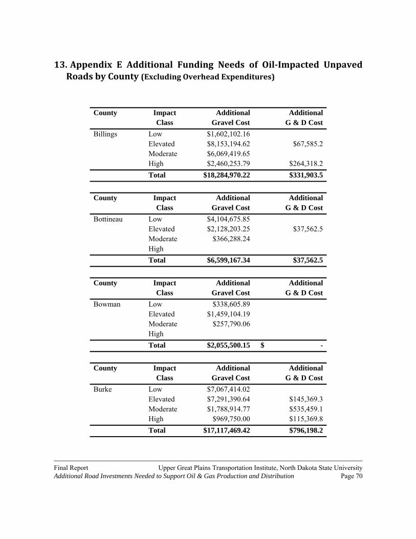
Final Report Upper Great Plains Transportation Institute, North Dakota State University Additional Road Investments Needed to Support Oil & Gas Production and Distribution Page 70
13. Appendix E Additional Funding Needs of Oil‐Impacted UnpavedRoadsbyCounty(ExcludingOverheadExpenditures)
County Impact Additional Additional Class Gravel Cost G & D Cost
Billings Low $1,602,102.16 Elevated $8,153,194.62 $67,585.2 Moderate $6,069,419.65 High $2,460,253.79 $264,318.2
Total $18,284,970.22 $331,903.5
County Impact Additional Additional Class Gravel Cost G & D Cost
Bottineau Low $4,104,675.85 Elevated $2,128,203.25 $37,562.5 Moderate $366,288.24 High
Total $6,599,167.34 $37,562.5
County Impact Additional Additional Class Gravel Cost G & D Cost
Bowman Low $338,605.89 Elevated $1,459,104.19 Moderate $257,790.06 High
Total $2,055,500.15 $ -
County Impact Additional Additional Class Gravel Cost G & D Cost
Burke Low $7,067,414.02 Elevated $7,291,390.64 $145,369.3 Moderate $1,788,914.77 $535,459.1 High $969,750.00 $115,369.8
Total $17,117,469.42 $796,198.2

Final Report Upper Great Plains Transportation Institute, North Dakota State University Additional Road Investments Needed to Support Oil & Gas Production and Distribution Page 71
County Impact Additional Additional Class Gravel Cost G & D Cost
Divide Low $1,909,826.89 Elevated $27,622,278.96 $133,562.5 Moderate $13,505,446.02 High $4,828,321.97 $261,575.8
Total $47,865,873.85 $395,138.3
County Impact Additional Additional Class Gravel Cost G & D Cost
Dunn Low $4,011,900.33 Elevated $39,627,107.28 $593,358.0 Moderate $20,821,531.72 $4,328,363.3 High $11,096,653.41 $484,915.4
Total $75,557,192.73 $5,406,636.6
County Impact Additional Additional Class Gravel Cost G & D Cost
Golden Valley Low $1,749,107.48 Elevated $14,976,909.06 $135,062.5 Moderate $5,007,291.83 $211,437.1 High $1,009,922.35
Total $22,743,230.71 $346,499.6
County Impact Additional Additional Class Gravel Cost G & D Cost
McHenry Low $1,034,003.94 Elevated $2,251,916.94 $111,693.2 Moderate High
Total $3,285,920.88 $111,693.2

Final Report Upper Great Plains Transportation Institute, North Dakota State University Additional Road Investments Needed to Support Oil & Gas Production and Distribution Page 72
County Impact Additional Additional Class Gravel Cost G & D Cost
McKenzie Low $5,082,926.70 Elevated $39,480,407.91 $361,772.7 Moderate $27,037,423.95 $2,585,429.3 High $10,022,047.35 $1,458,011.7
Total $81,622,805.91 $4,405,213.7
County Impact Additional Additional Class Gravel Cost G & D Cost
McLean Low $2,557,238.18 Elevated $6,550,254.75 $148,610.8 Moderate $5,589,228.62 $597,197.3 High $6,431,827.65 $370,896.3
Total $21,128,549.20 $1,116,704.4
County Impact Additional Additional Class Gravel Cost G & D Cost
Mercer Low $102,026.45 Elevated $370,322.39 Moderate $325,532.68 High
Total $797,881.52 $ -
County Impact Additional Additional Class Gravel Cost G & D Cost
Mountrail Low $6,738,804.55 Elevated $36,975,111.28 $83,809.7 Moderate $21,257,872.66 $292,730.0 High $11,096,782.26 $531,486.3
Total $76,068,570.74 $908,025.9

Final Report Upper Great Plains Transportation Institute, North Dakota State University Additional Road Investments Needed to Support Oil & Gas Production and Distribution Page 73
County Impact Additional Additional Class Gravel Cost G & D Cost
Renville Low $3,963,150.00 Elevated $1,025,572.79 $5,795.5 Moderate $1,735,587.85 $120,907.8 High $4,418,647.73 $464,803.8
Total $11,142,958.36 $591,507.1
County Impact Additional Additional Class Gravel Cost G & D Cost
Slope Low $144,601.06 Elevated $1,742,672.56 $78,431.8 Moderate $378,629.17 $180,367.1 High $194,276.52 $140.9
Total $2,460,179.31 $258,939.8
County Impact Additional Additional Class Gravel Cost G & D Cost
Stark Low $1,927,106.82 Elevated $19,242,781.26 $229,463.1 Moderate $9,897,180.93 $315,962.2 High $4,583,560.61 $312,350.1
Total $35,650,629.61 $857,775.4
County Impact Additional Additional Class Gravel Cost G & D Cost
Ward Low $2,229,152.46 Elevated $12,220,217.70 $167,801.1 Moderate $2,340,138.51 $301,850.3 High $12,488,270.83 $205,931.6
Total $29,277,779.51 $675,583.0

Final Report Upper Great Plains Transportation Institute, North Dakota State University Additional Road Investments Needed to Support Oil & Gas Production and Distribution Page 74
County Impact Additional Additional Class Gravel Cost G & D Cost
Williams Low $4,714,993.94 Elevated $47,439,991.56 $285,261.4 Moderate $32,638,679.07 $1,246,361.7 High $12,408,647.73 $374,306.1
Total $97,202,312.30 $1,905,929.1