Oil and Gas Supply Module of the National Energy Modeling ...2017).pdf · the National Energy...

Oil and Gas Supply Module of

the National Energy Modeling

System: Model Documentation

2017

February 2017

Independent Statistics & Analysis

www.eia.gov

U.S. Department of Energy

Washington, DC 20585

U.S. Energy Information Administration | NEMS Model Documentation 2017: Oil and Gas Supply Module i

This report was prepared by the U.S. Energy Information Administration (EIA), the statistical and

analytical agency within the U.S. Department of Energy. By law, EIA’s data, analyses, and forecasts are

independent of approval by any other officer or employee of the United States Government. The views

in this report therefore should not be construed as representing those of the Department of Energy or

other Federal agencies.

February 2017

U.S. Energy Information Administration | NEMS Model Documentation 2017: Oil and Gas Supply Module ii

Update Information

This edition of the Oil and Gas Supply Module of the National Energy Modeling System: Model

Documentation reflects changes made to the oil and gas supply module over the past couple of years for

the Annual Energy Outlook. The major revisions to the previous version of documentation include:

Corrected onshore drilling and completion cost equations.

Added a determination of the composition of natural gas plant liquids. (AEO2015)

Split light sweet crude into 3 crude type categories (35≤API gravity<40, 40≤API gravity<50, and

API gravity ≥ 50). (AEO2015)

Simplified the approach to modeling the impact of technology advancement on U.S. crude oil

and natural gas costs and productivity to better capture a continually changing technological

landscape. (AEO2016)

Updated county-level estimates of ultimate recovery per well for tight and shale formations

(Appendix 2.C). (AEO2016)

Updated offshore exploration and developmental drilling costs, operating costs, and

abandonment costs. (AEO2016)

Incorporated the dynamics of well productivity that occur as tighter well spacing in established

areas diminishes the productivity of each new well drilled. (AEO2017)

Updated assumptions for the announced/nonproducing offshore discoveries (Table 3-8).

(AEO2017)

Updated the undiscovered field size distribution for oil and natural gas resources in the Federal

Outer Continental Shelf (OCS) based on the Bureau of Ocean Energy Management (BOEM) 2016

assessment. (AEO2017)

February 2017

U.S. Energy Information Administration | NEMS Model Documentation 2017: Oil and Gas Supply Module iii

Table of Contents

Update Information ...................................................................................................................................... ii

1. Introduction .............................................................................................................................................. 1

Model purpose ........................................................................................................................................ 2

Model structure ....................................................................................................................................... 5

2. Onshore Lower 48 Oil and Gas Supply Submodule................................................................................... 7

Introduction ............................................................................................................................................. 7

Model purpose ........................................................................................................................................ 7

Resources modeled ........................................................................................................................... 7

Processes modeled ............................................................................................................................ 9

Major enhancements ........................................................................................................................ 9

Model structure ..................................................................................................................................... 11

Overall system logic ........................................................................................................................ 11

Known fields .................................................................................................................................... 12

Economics ....................................................................................................................................... 14

Timing .............................................................................................................................................. 51

Project selection .............................................................................................................................. 53

Constraints ...................................................................................................................................... 59

Technology ...................................................................................................................................... 66

Appendix 2.A: Onshore Lower 48 Data Inventory ...................................................................................... 66

Appendix 2.B: Cost and Constraint Estimation ........................................................................................... 96

Appendix 2.C: Decline Curve Analysis ....................................................................................................... 166

Appendix 2.D: Representation of Power Plant and xTL Captured CO2 in EOR ......................................... 173

Modification of EOR project constraints in OGSM .............................................................................. 175

Integration of EMM into CO2 EOR process .......................................................................................... 176

Mathematical description of EMM-CTUS constraints ......................................................................... 176

Integration of LFMM into CO2 EOR process ........................................................................................ 177

Mathematical description of LFMM-CTUS constraints ........................................................................ 178

3. Offshore Oil and Gas Supply Submodule .............................................................................................. 180

Introduction ......................................................................................................................................... 180

Undiscovered fields component .......................................................................................................... 180

Discovered undeveloped fields component ........................................................................................ 196

February 2017

U.S. Energy Information Administration | NEMS Model Documentation 2017: Oil and Gas Supply Module iv

Producing fields component ................................................................................................................ 198

Generation of supply curves ................................................................................................................ 200

Advanced technology impacts ............................................................................................................. 201

Appendix 3.A. Offshore data inventory ................................................................................................... 202

4. Alaska Oil and Gas Supply Submodule .................................................................................................. 212

AOGSS overview .................................................................................................................................. 212

Calculation of costs ...................................................................................................................... 214

Discounted cash flow analysis ............................................................................................................. 217

New field discovery .............................................................................................................................. 219

Development projects ......................................................................................................................... 221

Producing fields ................................................................................................................................... 222

Appendix 4.A. Alaskan Data Inventory ..................................................................................................... 225

5. Oil Shale Supply Submodule ................................................................................................................. 227

Oil shale facility cost and operating parameter assumptions ............................................................. 231

Appendix A. Discounted Cash Flow Algorithm ......................................................................................... 242

Appendix B. Bibliography ......................................................................................................................... 255

Appendix C. Model Abstract .................................................................................................................... 269

Appendix D. Output Inventory ................................................................................................................. 273

February 2017

U.S. Energy Information Administration | NEMS Model Documentation 2017: Oil and Gas Supply Module v

Tables

Table 2-1. Processes modeled by OLOGSS .................................................................................................... 9

Table 2-2. Costs applied to crude oil processes .......................................................................................... 22

Table 2-3. Costs applied to natural gas processes ...................................................................................... 23

Table 2-4. EOR/ASR eligibility ranges .......................................................................................................... 52

Table 2-5. Rig depth categories .................................................................................................................. 63

Table 2-6. Onshore lower 48 technology assumptions .............................................................................. 66

Table 2.C-1. Hyperbolic decline curve parameters for select tight oil plays ............................................ 167

Table 2.C-2. Hyperbolic decline curve parameters for select shale gas plays .......................................... 170

Table 2.D- 1. Inventory of Variables Passed Between CTUS, OGSM, EMM and LFMM ............................ 175

Table 3-1. Offshore region and evaluation unit crosswalk ....................................................................... 181

Table 3-2. Number of undiscovered fields by evaluation unit and field size class, as of 1/1/2003 ......... 183

Table 3-3. Field size definition .................................................................................................................. 184

Table 3-4. Production facility by water depth level .................................................................................. 190

Table 3-5. Well completion and equipment costs per well ...................................................................... 191

Table 3-6. Production facility design, fabrication, and installation period (years) ................................... 194

Table 3-7. Development drilling capacity by production facility type ...................................................... 195

Table 3-8. Assumed size and initial production year of major announced deepwater discoveries ......... 197

Table 3-9. Production profile data for oil & gas producing fields ............................................................. 199

Table 3-10. Offshore exploration and production technology levers ....................................................... 201

Table 4-1. AOGSS oil well drilling and completion costs by location and category .................................. 215

Table 5-1. OSSS oil shale facility configuration and cost parameters ....................................................... 232

Table 5-2. OSSS oil shale facility electricity consumption and natural gas production parameters and

their prices and costs ................................................................................................................................ 233

Table 5-3. Discount rate financial parameters .......................................................................................... 237

Table 5-4. Market penetration parameters .............................................................................................. 239

Table A-1. Tax treatment in oil and gas production by category of company under current tax

legislation .................................................................................................................................................. 249

Table A-2. MACRS schedules..................................................................................................................... 252

February 2017

U.S. Energy Information Administration | NEMS Model Documentation 2017: Oil and Gas Supply Module vi

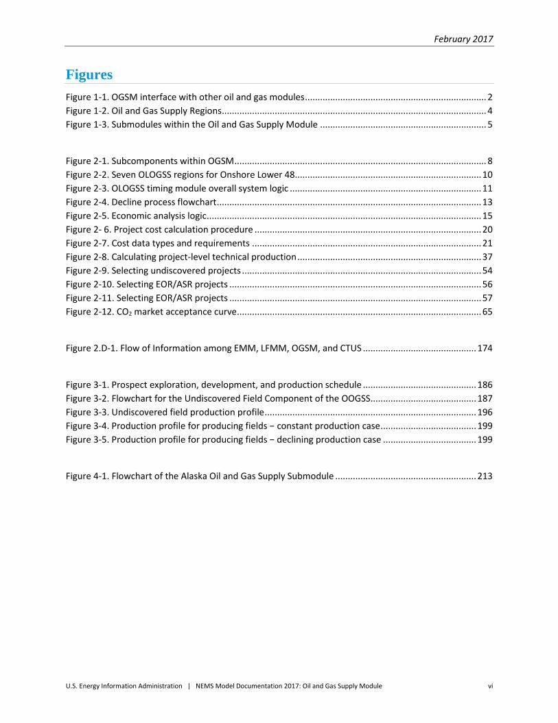
Figures

Figure 1-1. OGSM interface with other oil and gas modules ........................................................................ 2

Figure 1-2. Oil and Gas Supply Regions ......................................................................................................... 4

Figure 1-3. Submodules within the Oil and Gas Supply Module .................................................................. 5

Figure 2-1. Subcomponents within OGSM .................................................................................................... 8

Figure 2-2. Seven OLOGSS regions for Onshore Lower 48.......................................................................... 10

Figure 2-3. OLOGSS timing module overall system logic ............................................................................ 11

Figure 2-4. Decline process flowchart ......................................................................................................... 13

Figure 2-5. Economic analysis logic ............................................................................................................. 15

Figure 2- 6. Project cost calculation procedure .......................................................................................... 20

Figure 2-7. Cost data types and requirements ........................................................................................... 21

Figure 2-8. Calculating project-level technical production ......................................................................... 37

Figure 2-9. Selecting undiscovered projects ............................................................................................... 54

Figure 2-10. Selecting EOR/ASR projects .................................................................................................... 56

Figure 2-11. Selecting EOR/ASR projects .................................................................................................... 57

Figure 2-12. CO2 market acceptance curve ................................................................................................. 65

Figure 2.D-1. Flow of Information among EMM, LFMM, OGSM, and CTUS ............................................. 174

Figure 3-1. Prospect exploration, development, and production schedule ............................................. 186

Figure 3-2. Flowchart for the Undiscovered Field Component of the OOGSS .......................................... 187

Figure 3-3. Undiscovered field production profile .................................................................................... 196

Figure 3-4. Production profile for producing fields − constant production case ...................................... 199

Figure 3-5. Production profile for producing fields − declining production case ..................................... 199

Figure 4-1. Flowchart of the Alaska Oil and Gas Supply Submodule ........................................................ 213

February 2017

U.S. Energy Information Administration | NEMS Model Documentation 2017: Oil and Gas Supply Module 1

1. Introduction

The purpose of this report is to define the objectives of the Oil and Gas Supply Module (OGSM), to describe the model's basic approach, and to provide detail on how the model works. This report is intended as a reference document for model analysts, users, and the public. It is prepared in accordance with the U.S. Energy Information Administration's (EIA) legal obligation to provide adequate documentation in support of its statistical and forecast reports (Public Law 93-275, Section 57(b)(2)).

Projected production estimates of U.S. crude oil and natural gas are based on supply functions generated endogenously within the National Energy Modeling System (NEMS) by the OGSM. The OGSM encompasses both conventional and unconventional domestic crude oil and natural gas supply. Crude oil and natural gas projections are further disaggregated by geographic region. The OGSM projects U.S. domestic oil and gas supply for six Lower 48 onshore regions, three offshore regions, and Alaska. The general methodology relies on forecast profitability to determine exploratory and developmental drilling levels for each region and fuel type. These projected drilling levels translate into reserve additions, as well as a modification of the production capacity for each region.

The OGSM utilizes both exogenous input data and data from other modules within NEMS. The primary exogenous inputs are resource levels, finding-rate parameters, costs, production profiles, and tax rates − all of which are critical determinants of the expected returns from projected drilling activities. Regional projections of natural gas wellhead prices and production are provided by the Natural Gas Transmission and Distribution Module (NGTDM). Projections of the crude oil wellhead prices at the OGSM regional level come from the Liquid Fuels Market Model (LFMM). Important economic factors, namely interest rates and gross domestic product (GDP) deflators, flow to the OGSM from the Macroeconomic Activity Module (MAM). Controlling information (e.g., forecast year) and expectations information (e.g., expected price paths) come from the Integrating Module (i.e. system module).

Outputs from the OGSM go to other oil and gas modules (NGTDM and LFMM) and to other modules of NEMS. To equilibrate supply and demand in the given year, the NGTDM employs short-term supply functions (with the parameters provided by the OGSM) to determine non-associated gas production and natural gas imports. Crude oil production is determined within the OGSM using short-term supply functions, which reflect potential oil or gas flows to the market for a one-year period. The gas functions are used by the NGTDM and the oil volumes are used by the LFMM for the determination of equilibrium prices and quantities of crude oil and natural gas at the wellhead. The OGSM also provides projections of natural gas plant liquids production to the LFMM. Other NEMS modules receive projections of selected OGSM variables for various uses. Oil and gas production is passed to the Integrating Module for reporting purposes. Forecasts of oil and gas production are also provided to the MAM to assist in forecasting aggregate measures of output

February 2017


Model purpose The OGSM is a comprehensive framework used to analyze oil and gas supply potential and related

issues. Its primary function is to produce domestic projections of crude oil and natural gas production as

well as natural gas imports and exports in response to price data received endogenously (within NEMS)

from the NGTDM and LFMM. Projected natural gas and crude oil wellhead prices are determined within

the NGTDM and LFMM, respectively. As the supply component only, the OGSM cannot project prices,

which are the outcome of the equilibration of both demand and supply.

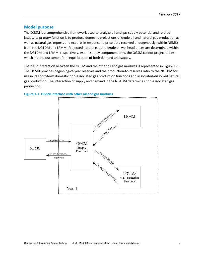
The basic interaction between the OGSM and the other oil and gas modules is represented in Figure 1-1.

The OGSM provides beginning-of-year reserves and the production-to-reserves ratio to the NGTDM for

use in its short-term domestic non-associated gas production functions and associated-dissolved natural

gas production. The interaction of supply and demand in the NGTDM determines non-associated gas

production.

Figure 1-1. OGSM interface with other oil and gas modules

February 2017


The OGSM provides domestic crude oil production to the LFMM. The interaction of supply and demand

in the LFMM determines the level of imports. System control information (e.g., forecast year) and

expectations (e.g., expected price paths) come from the Integrating Module. Major exogenous inputs

include resource levels, finding-rate parameters, costs, production profiles, and tax rates − all of which

are critical determinants of the oil and gas supply outlook of the OGSM.

The OGSM operates on a regionally disaggregated level, further differentiated by fuel type. The basic

geographic regions are Lower 48 onshore, Lower 48 offshore, and Alaska, each of which, in turn, is

divided into a number of subregions (see Figure 1-2). The primary fuel types are crude oil and natural

gas, which are further disaggregated based on type of deposition, method of extraction, or geologic

formation. Crude oil supply includes lease condensate. Natural gas is differentiated by non-associated

and associated-dissolved gas.1 Non-associated natural gas is categorized by fuel type: high-permeability

carbonate and sandstone (conventional), low-permeability carbonate and sandstone (tight gas), shale

gas, and coalbed methane.

The OGSM provides mid-term (currently through year 2040) projections and serves as an analytical tool

for the assessment of alternative supply policies. One publication that utilizes OGSM forecasts is the

Annual Energy Outlook (AEO). Analytical issues that OGSM can address involve policies that affect the

profitability of drilling through impacts on certain variables, including:

drilling and production costs

regulatory or legislatively mandated environmental costs

key taxation provisions such as severance taxes, state or federal income taxes, depreciation

schedules and tax credits

the rate of penetration for different technologies into the industry by fuel type

The cash flow approach to the determination of drilling levels enables the OGSM to address some

financial issues. In particular, the treatment of financial resources within the OGSM allows for explicit

consideration of the financial aspects of upstream capital investment in the petroleum industry.

The OGSM is also useful for policy analysis of resource base issues. OGSM analysis is based on explicit

estimates for technically recoverable oil and gas resources for each of the sources of domestic

production (i.e., geographic region/fuel type combinations). With some modification, this feature could

allow the model to be used for the analysis of issues involving:

the uncertainty surrounding the technically recoverable oil and gas resource estimates

access restrictions on much of the offshore Lower 48 states, the wilderness areas of the onshore

Lower 48 states, and the 1002 Study Area of the Arctic National Wildlife Refuge (ANWR).

1 Non-associated (NA) natural gas is gas not in contact with significant quantities of crude oil in a reservoir. Associated-

dissolved natural gas consists of the combined volume of natural gas that occurs in crude oil reservoirs either as free gas

(associated) or as gas in solution with crude oil (dissolved).

February 2017


Figure 1-2. Oil and Gas Supply Regions

February 2017


Model structure The OGSM consists of a set of submodules (Figure 1-3) and is used to perform supply analysis of

domestic oil and gas as part of NEMS. The OGSM provides crude oil production and parameter estimates

representing natural gas supplies by selected fuel types on a regional basis to support the market

equilibrium determination conducted within other modules of NEMS. The oil and gas supplies in each

period are balanced against the regionally-derived demand for the produced fuels to solve

simultaneously for the market clearing prices and quantities in the wellhead and end-use markets. The

description of the market analysis models may be found in the separate methodology documentation

reports for the LFMM and the NGTDM.

The OGSM represents the activities of firms that produce oil and natural gas from domestic fields

throughout the United States. The OGSM encompasses domestic crude oil and natural gas supply by

both conventional and unconventional recovery techniques. Natural gas is categorized by fuel type:

high-permeability carbonate and sandstone (conventional), low-permeability carbonate and sandstone

(tight gas), shale gas, and coalbed methane. Unconventional oil includes production of synthetic crude

from oil shale (syncrude). Crude oil and natural gas projections are further disaggregated by geographic

region. Liquefied natural gas (LNG) imports and pipeline natural gas import/export trade with Canada

and Mexico are determined in the NGTDM.

Figure 1-3. Submodules within the Oil and Gas Supply Module

February 2017


The model’s methodology is shaped by the basic principle that the level of investment in a specific

activity is determined largely by its expected profitability. Output prices influence oil and gas supplies in

distinctly different ways in the OGSM. Quantities supplied as the result of the annual market

equilibration in the LFMM and the NGTDM are determined as a direct result of the observed market

price in that period. Longer-term supply responses are related to investments required for subsequent

production of oil and gas. Output prices affect the expected profitability of these investment

opportunities as determined by use of a discounted cash flow evaluation of representative prospects.

The OGSM incorporates a complete and representative description of the processes by which oil and gas

in the technically recoverable resource base2 convert to prove reserves.3

The breadth of supply processes that are encompassed within OGSM result in different methodological

approaches for determining crude oil and natural gas production from Lower 48 onshore, Lower 48

offshore, Alaska, and oil shale. The present OGSM consequently comprises four submodules. The

Onshore Lower 48 Oil and Gas Supply Submodule (OLOGSS) models crude oil and natural gas supply

from resources in the Lower 48 States. The Offshore Oil and Gas Supply Submodule (OOGSS) models oil

and gas exploration and development in the offshore Gulf of Mexico, Pacific, and Atlantic regions. The

Alaska Oil and Gas Supply Submodule (AOGSS) models industry supply activity in Alaska. Oil shale

(synthetic) is modeled in the Oil Shale Supply Submodule (OSSS). The distinctions of each submodule are

explained in individual chapters covering methodology. Following the methodology chapters, four

appendices are included: Appendix A provides a description of the discounted cash flow (DCF)

calculation; Appendix B is the bibliography; Appendix C contains a model abstract; and Appendix D is an

inventory of key output variables.

2 Technically recoverable resources are those volumes considered to be producible with current recovery technology and

efficiency but without reference to economic viability. Technically recoverable volumes include proved reserves and inferred

reserves as well as undiscovered and other unproved resources. These resources may be recoverable by techniques considered

either conventional or unconventional. 3 Proved reserves are the estimated quantities that analyses of geological and engineering data demonstrate with reasonable

certainty to be recoverable in future years from known reservoirs under existing economic and operating conditions.

February 2017


2. Onshore Lower 48 Oil and Gas Supply Submodule

Introduction U.S. onshore lower 48 crude oil and natural gas supply projections are determined by the Onshore

Lower 48 Oil and Gas Supply Submodule (OLOGSS). The general methodology relies on a detailed

economic analysis of potential projects in known crude oil and natural gas fields, enhanced oil recovery

projects, developing natural gas plays, and undiscovered crude oil and natural gas resources. The

projects that are economically viable are developed subject to resource development constraints which

simulate the existing and expected infrastructure of the oil and gas industries. The economic production

from the developed projects is aggregated to the regional and national levels.

The OLOGSS utilizes both exogenous input data and data from other modules within the National Energy

Modeling System (NEMS). The primary exogenous data includes technical production for each project

considered, cost and development constraint data, tax information, and project development data.

Regional projections of natural gas wellhead prices and production are provided by the NGTDM. From

the LFMM come projections of crude oil wellhead prices at the OGSM regional level.

Model purpose OLOGSS is a comprehensive model with which to analyze crude oil and natural gas supply potential and

related economic issues. Its primary purpose is to project production of crude oil and natural gas from

the onshore lower 48 in response to price data received from the LFMM and the NGTDM. As a supply

submodule, OLOGSS does not project prices.

The basic interaction between OLOGSS and the OGSM is illustrated in Figure 2-1. As seen in the figure,

OLOGSS models the entirety of the domestic crude oil and natural gas production within the onshore

lower 48.

Resources modeled

Crude oil resources

Crude oil resources, as illustrated in Figure 2-1, are divided into known fields and undiscovered fields.

For known resources, exogenous production-type curves are used for quantifying the technical

production profiles from known fields under primary, secondary, and tertiary recovery processes.

Primary resources are also quantified for their advanced secondary recovery (ASR) processes, including

waterflooding, infill drilling, horizontal continuity, and horizontal profile modification. Known resources

are evaluated for the potential they may possess when employing enhanced oil recovery (EOR)

processes such as CO2 flooding, steam flooding, polymer flooding and profile modification. Known

crude oil resources include highly fractured continuous zones such as the Austin chalk formations and

the Bakken shale formations.

February 2017


Figure 2-1. Subcomponents within OGSM

Undiscovered crude oil resources are characterized in a method similar to that used for discovered

resources and are evaluated for their potential production from primary and secondary techniques. The

potential from an undiscovered resource is defined based on United States Geological Survey (USGS)

estimates and is distinguished as either conventional or continuous. Conventional crude oil and natural

gas resources are defined as discrete fields with well-defined hydrocarbon-water contacts, where the

hydrocarbons are buoyant on a column of water. Conventional resources commonly have relatively high

permeability and obvious seals and traps. In contrast, continuous resources commonly are regional in

extent, have diffuse boundaries, and are not buoyant on a column of water. Continuous resources have

very low permeability, do not have obvious seals and traps, are in close proximity to source rocks, and

are abnormally pressured. Included in the category of continuous accumulations are hydrocarbons that

occur in tight reservoirs, shale reservoirs, fractured reservoirs, and coal beds.

Natural gas resources

Natural gas resources, as illustrated in Figure 2-1, are divided into known producing fields, developing

natural gas plays, and undiscovered fields. Exogenous production-type curves have been used to

estimate the technical production from known fields. The undiscovered resources have been

characterized based on resource estimates developed by the USGS. Existing databases of developing

plays, such as the Marcellus Shale, have been incorporated into the model’s resource base. The natural

gas resource estimates have been developed from detailed geological characterizations of producing

plays.

February 2017


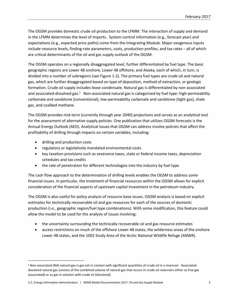
Processes modeled

OLOGSS models primary, secondary and tertiary oil recovery processes. For natural gas, OLOGSS models

discovered and undiscovered fields, as well as discovered and developing fields. Table 2-1 lists the

processes modeled by OLOGSS.

Table 2-1. Processes modeled by OLOGSS

Crude Oil Processes Natural Gas Processes

Existing Fields and Reservoirs

Waterflooding in Undiscovered Resources

CO2 Flooding

Steam Flooding

Polymer Flooding

Infill Drilling

Profile Modification

Horizontal Continuity

Horizontal Profile

Undiscovered Conventional

Undiscovered Continuous

Existing Radial Flow

Existing Water Drive

Existing Tight Sands

Existing Dry Coal/Shale

Existing Wet Coal/Shale

Undiscovered Conventional

Undiscovered Tight Gas

Undiscovered Coalbed Methane

Undiscovered Shale Gas

Developing Shale Gas

Developing Coalbed Methane

Developing Tight Gas

Major enhancements

OLOGSS is a play-level model that projects the crude oil and natural gas supply from the onshore lower

48. The modeling procedure includes a comprehensive assessment method for determining the relative

economics of various prospects based on future financial considerations, the nature of the undiscovered

and discovered resources, prevailing risk factors, and the available technologies. The model evaluates

the economics of future exploration and development from the perspective of an operator making an

investment decision. Technological advances, including improved drilling and completion practices as

well as advanced production and processing operations, are explicitly modeled to determine the direct

impacts on supply, reserves, and various economic parameters. The model is able to evaluate the

impact of research and development (R&D) on supply and reserves. Furthermore, the model design

provides the flexibility to evaluate alternative or new taxes, environmental, or other policy changes in a

consistent and comprehensive manner.

OLOGSS provides a variety of levers that allow the user to model developments affecting the

profitability of development:

Development of new technologies

Rate of market penetration of new technologies

Costs to implement new technologies

Impact of new technologies on capital and operating costs

Regulatory or legislative environmental mandates

February 2017


In addition, OLOGSS can quantify the effects of hypothetical developments that affect the resource

base. OLOGSS is based on explicit estimates for technically recoverable crude oil and natural gas

resources for each source of domestic production (i.e., geographic region/fuel type combinations).

OLOGSS can be used to analyze access issues concerning crude oil and natural gas resources located on

federal lands. Undiscovered resources are divided into four categories:

Officially inaccessible

Inaccessible due to development constraints

Accessible with federal lease stipulations

Accessible under standard lease terms

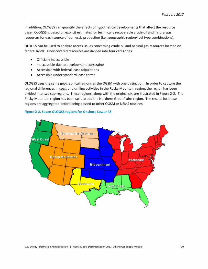
OLOGSS uses the same geographical regions as the OGSM with one distinction. In order to capture the

regional differences in costs and drilling activities in the Rocky Mountain region, the region has been

divided into two sub-regions. These regions, along with the original six, are illustrated in Figure 2-2. The

Rocky Mountain region has been split to add the Northern Great Plains region. The results for these

regions are aggregated before being passed to other OGSM or NEMS routines.

Figure 2-2. Seven OLOGSS regions for Onshore Lower 48

February 2017


Model structure The OLOGSS projects the annual crude oil and natural gas production from existing fields, reserves

growth, and exploration. It performs economic evaluation of the projects and ranks the reserves growth

and exploration projects for development in a way designed to mimic the way decisions are made by the

oil and gas industry. Development decisions and project selection depend upon economic viability and

the competition for capital, drilling, and other available development constraints. Finally, the model

aggregates production and drilling statistics using geographical and resource categories.

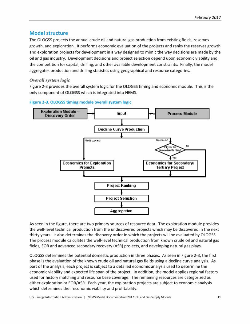
Overall system logic

Figure 2-3 provides the overall system logic for the OLOGSS timing and economic module. This is the

only component of OLOGSS which is integrated into NEMS.

Figure 2-3. OLOGSS timing module overall system logic

As seen in the figure, there are two primary sources of resource data. The exploration module provides the well-level technical production from the undiscovered projects which may be discovered in the next thirty years. It also determines the discovery order in which the projects will be evaluated by OLOGSS. The process module calculates the well-level technical production from known crude oil and natural gas fields, EOR and advanced secondary recovery (ASR) projects, and developing natural gas plays.

OLOGSS determines the potential domestic production in three phases. As seen in Figure 2-3, the first phase is the evaluation of the known crude oil and natural gas fields using a decline curve analysis. As part of the analysis, each project is subject to a detailed economic analysis used to determine the economic viability and expected life span of the project. In addition, the model applies regional factors used for history matching and resource base coverage. The remaining resources are categorized as either exploration or EOR/ASR. Each year, the exploration projects are subject to economic analysis which determines their economic viability and profitability.

February 2017


For the EOR/ASR projects, development eligibility is determined before the economic analysis is

conducted. The eligibility is based upon the economic life span of the corresponding decline curve

project and the process-specific eligibility window. If a project is not currently eligible, it will be re-

evaluated in future years. The projects which are eligible are subject to the same type of economic

analysis applied to existing and exploration projects in order to determine the viability and relative

profitability of the project.

After the economics have been determined for each eligible project, the projects are sorted. The

exploration projects maintain their discovery order. The EOR/ASR projects are sorted by their relative

profitability. The finalized lists are then considered by the project selection routines.

A project will be selected for development only if it is economically viable and if there are sufficient

development resources available to meet the project’s requirements. Development resource

constraints are used to simulate limits on the availability of infrastructure related to the oil and gas

industries. If sufficient resources are not available for an economic project, the project will be

reconsidered in future years if it remains economically viable. Other development options are

considered in this step, including the waterflooding of undiscovered conventional resources and the

extension of CO2 floods through an increase in total pore volume injected.

The production, reserves, and other key parameters for the timed and developed projects are

aggregated at the regional and national levels.

The remainder of this document provides additional details on the logic and particular calculations for

each of these steps. These include the decline analysis, economic analysis, timing decisions, project

selection, constraints, and modeling of technology.

Known fields

In this step, the production from existing crude oil and natural gas projects is estimated. A detailed

economic analysis is conducted in order to calculate the economically viable production as well as the

expected life of each project. The project life is used to determine when a project becomes eligible for

EOR and ASR processes.

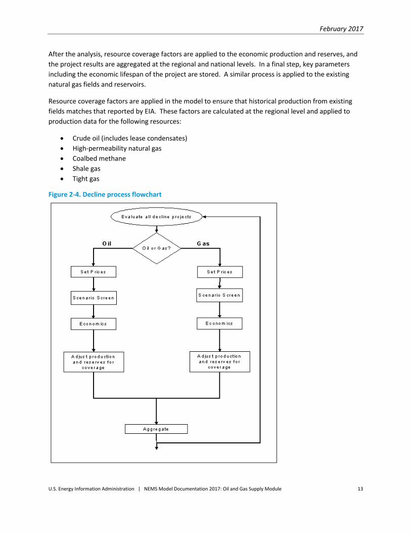
The logic for this process is provided in Figure 2-4. For each crude oil project, regional prices are set and

the project is screened to determine whether the user has specified any technology and/or economic

levers. The screening considers factors including region, process, depth, and several other petro-

physical properties. After applicable levers are determined, the project undergoes a detailed economic

analysis.

February 2017


After the analysis, resource coverage factors are applied to the economic production and reserves, and

the project results are aggregated at the regional and national levels. In a final step, key parameters

including the economic lifespan of the project are stored. A similar process is applied to the existing

natural gas fields and reservoirs.

Resource coverage factors are applied in the model to ensure that historical production from existing

fields matches that reported by EIA. These factors are calculated at the regional level and applied to

production data for the following resources:

Crude oil (includes lease condensates)

High-permeability natural gas

Coalbed methane

Shale gas

Tight gas

Figure 2-4. Decline process flowchart

February 2017


Economics

Project costs

OLOGSS conducts the economic analysis of each project using regional crude oil and natural gas prices.

After these prices are set, the model evaluates the base and advanced technology cases for the project.

The base case is defined as the current technology and cost scenario for the project, while the advanced

case includes technology and/or cost improvements associated with the application of model levers. It

is important to note that these cases – for which the assumptions are applied to data for the project –

are not the same as the AEO low, reference, or high technology cases.

For each technology case, the necessary petro-physical properties and other project data are set, the

regional dryhole rates are determined, and the process-specific depreciation schedule is assigned. The

capital and operating costs for the project are then calculated and aggregated for both the base and

advanced technology cases.

In the next step, a standard cash flow analysis is conducted, the discounted rate of return is calculated,

and the ranking criteria are set for the project. Afterwards, the number and type of wells required for

the project and the last year of actual economic production are set. Finally, the economic variables,

including production, development requirements, and other parameters, are stored for project timing

and aggregation. All of these steps are illustrated in Figure 2-5.

The details of the calculations used in conducting the economic analysis of a project are provided in the

following description.

Determine the project shift: The first step is to determine the number of years the project development

is shifted, i.e., the number of years between the discovery of a project and the start of its development.

This will be used to determine the crude oil and natural gas price shift. The number of years is

dependent upon both the development schedule – when the project drilling begins – and upon the

process.

Determine annual prices: Determine the annual prices used in evaluating the project. Crude oil and

natural gas prices in each year use the average price for the previous five years.

Begin analysis of base and advanced technology: To capture the impacts of technological improvements

on both production and economics, the model divides the project into two categories. The first category

– base technology – does not include improvements associated with technology or economic levers.

The second category – advanced technology – incorporates the impact of the levers. The division of the

project depends on the market penetration algorithm of any applicable technologies.

Determine the dryhole rate for the project: Assigns the regional dryhole rates for undiscovered

exploration, undiscovered development, and discovered development. Three types of dryhole rates are

used in the model: development in known fields and reservoirs, the first (wildcat) well in an exploration

project, and subsequent wells in an exploration project. Specific dryhole rates are used for horizontal

drilling and the developing natural gas resources.

February 2017


Figure 2-5. Economic analysis logic

February 2017


In the advanced case, the dryhole rates may also incorporate technology improvements associated with

exploration or drilling success.

itechitechim

itechim, EXPLR_FAC*DRILL_FAC0.1*100

SUCEXPREGDRYUE

(2-1)

itechim

itechim, DRILL_FAC0.1*100

SUCEXPDREGDRYUD

(2-2)

itechim


SUCDEVEREGDRYKD

(2-3)

If evaluating horizontal continuity or horizontal profile, then,

itechim


SUCCHDEVREGDRYKD

(2-4)

If evaluating developing natural gas resources, then,

itechiresitechim, DRILL_FAC0.1*ALATNUMREGDRYUD (2-5)

where

itech = Technology case number

im = Region number

REGDRYUE = Project-specific dryhole rate for undiscovered exploration

(Wildcat)

REGDRYUD = Project-specific dryhole rate for undiscovered development

REGDRYKD = Project-specific dryhole rate for known field development

SUCEXPD = Regional dryhole rate for undiscovered development

ALATNUM = Variable representing the regional dryhole rate for known

field development

SUCDEVE = Regional dryhole rate for undiscovered exploration (Wildcat)

SUCCDEVH = Dryhole rate for horizontal drilling

DRILL_FAC = Technology lever applied to dryhole rate

EXPLR_FAC = Technology factor applied to exploratory dryhole rate

February 2017


Process-specific depreciation schedule: The default depreciation schedule is based on an eight-year declining balance depreciation method. The user may select process-specific depreciation schedules for CO2 flooding, steam flooding, or water flooding in the input file.

Calculate the capital and operating costs for the project: The project costs are calculated for each technology case. The costs are specific to crude oil or natural gas resources. The results of the cost calculations, which include technical crude oil and natural gas production, as well as drilling costs, facilities costs, and operating costs, are then aggregated to the project level.

G & G factor: Calculates the geological and geophysical (G&G) factor for each technology case. This is added to the first year cost.

GG_FAC*INTANG_M*DRL_CSTGGGGitech itechitechitech (2-6)

where

GGitech = Geophysical and Geological costs for the first year of the

project

DRL_CSTitech = Total drilling cost for the first year of the project

INTANG_Mitech = Energy Elasticity factor for intangible investments (first year)

GG_FAC = Portion of exploratory costs that is G&G costs

After the variables are aggregated, the technology case loop ends. At this point, the process-specific capital costs, which apply to the entire project instead of the technology case, are calculated.

Cash flow Analysis: The model then conducts a cash flow analysis on the project and calculates the discounted rate of return. Economic Analysis is conducted using a standard cash flow routine described in Appendix A.

Calculate the discounted rate of return: Determines the projected rate of return for all investments and production. The cumulative investments and discounted after-tax cash flow are used to calculate the investment efficiency for the project.

Calculate wells: The annual number of new and existing wells is calculated for the project. The model tracks five drilling categories:

New production wells drilled

New injection wells drilled

Active production wells

Active injection wells

Shut-in wells

February 2017


The calculation of the annual well count depends on the number of existing production and injection wells as well as on the process and project-specific requirements to complete each drilling pattern developed.

Determine number of years a project is economic: The model calculates the last year of actual

economic production. This is based on the results of the cash flow analysis. The last year of production

is used to determine the aggregation range to be used if the project is selected for development.

If the project is economic only in the first year, it will be considered uneconomic and unavailable for

development at that time. If this occurs for an existing crude oil or natural gas project, the model will

assume that all of the wells will be shut in.

Non-producing decline project: Determines if the existing crude oil or natural gas project is non-

producing. If there is no production, then the end point for project aggregation is not calculated. This

check applies only to the existing crude oil and natural gas projects.

Ranking criteria: Ranks investment efficiency based on the discounted after tax cash flow over tangible

and intangible investments.

Determine ranking criterion: The ranking criterion, specified by the user, is the parameter by which the

projects will be sorted before development. Ranking criteria options include the project net present

value, the rate of return for the project, and the investment efficiency.

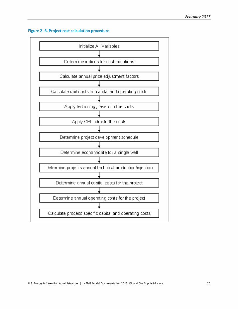
Calculating Unit Costs

To conduct the cost analysis, the model calculates price adjustment factors as well as unit costs for all

required capital and operating costs. Unit costs include the cost of drilling and completing a single well,

producing one barrel of crude oil, or operating one well for a year. These costs are adjusted using the

technology levers and Consumer Price Index (CPI). After the development schedule for the project is

determined and the economic life of a single well is calculated, the technical production and injection

are determined for the project. Based on the project’s development schedule and the technical

production, the annual capital and operating costs are determined. In the final step, the process- and

resource-specific capital and operating costs are calculated for the project. These steps are illustrated in

Figure 2-6.

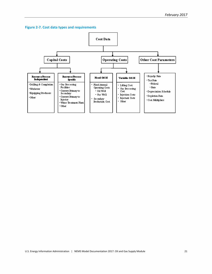
The Onshore Lower 48 Oil and Gas Supply Submodule uses detailed project costs for economic

calculations. There are three broad categories of costs used by the model: capital costs, operating costs,

and other costs. These costs are illustrated in Figure 2-7. Capital costs encompass the costs of drilling

and equipment necessary for the production of crude oil and natural gas resources. Operating costs are

used to calculate the full life cycle economics of the project. Operating costs consist of normal daily

expenses and surface maintenance. Other cost parameters include royalty, state and federal taxes, and

other required schedules and factors.

February 2017


The calculations for capital costs and operating costs for both crude oil and natural gas are described in

detail below. The capital and operating costs are used in the timing and economic module to calculate

the lifecycle economics for all crude oil and natural gas projects.

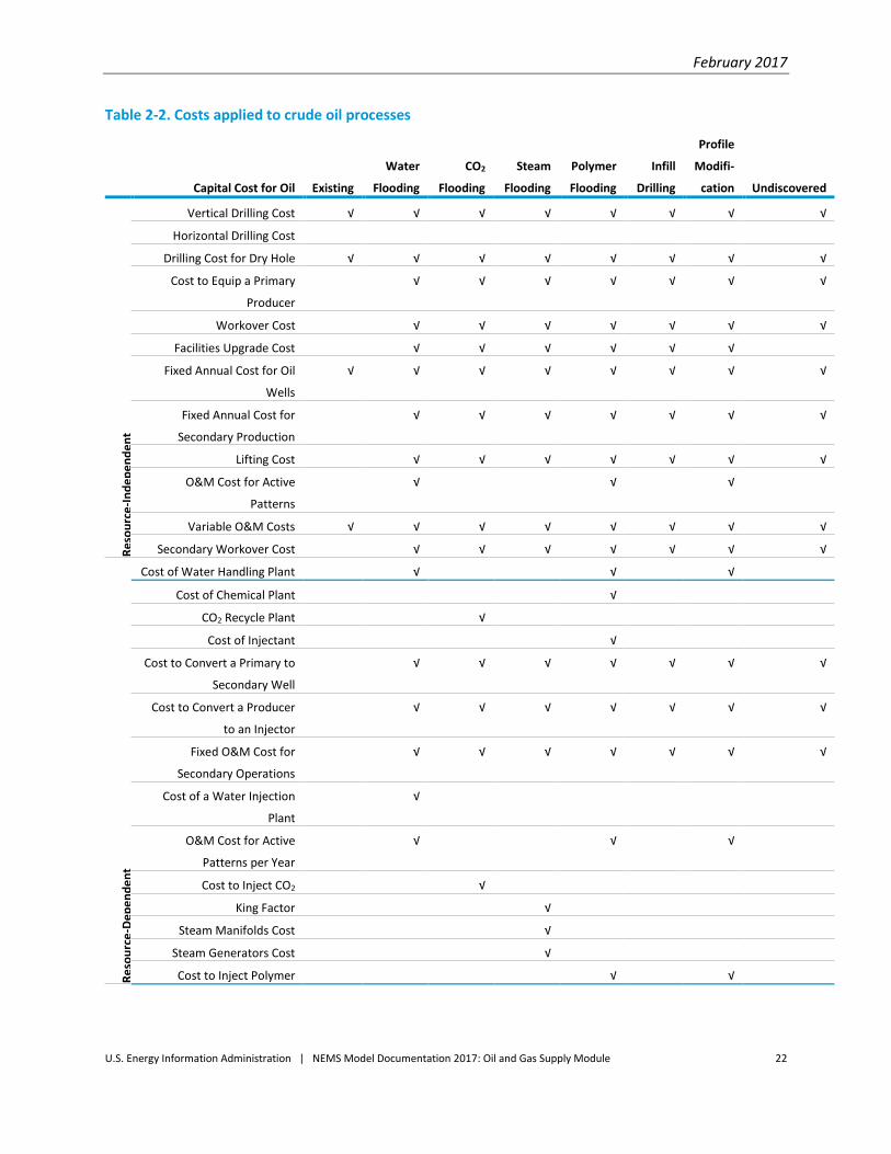
There are two categories for these costs: costs that are applied to all processes, thus defined as

resource-independent, and the process-specific, or resource-dependent costs. Resource-dependent

costs are used to calculate the economics for existing, reserves growth, and exploration projects. The

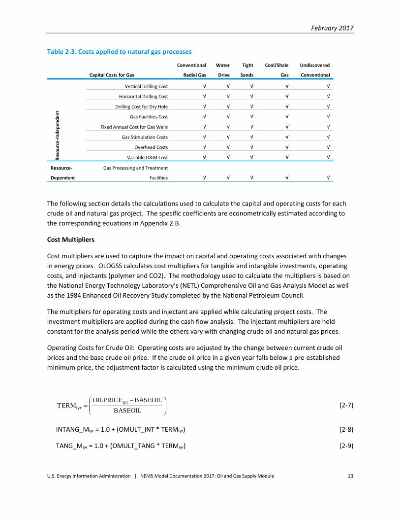
capital costs for both crude oil and natural gas are calculated first, followed by the resource-independent costs, and then the resource-dependent costs.

The resource-independent and resource-dependent costs applied to each of the crude oil and natural gas processes are detailed in Tables 2-2 and 2-3 respectively.

February 2017


Figure 2- 6. Project cost calculation procedure

February 2017


Figure 2-7. Cost data types and requirements

February 2017


Table 2-2. Costs applied to crude oil processes

Capital Cost for Oil Existing

Water

Flooding

CO2

Flooding

Steam

Flooding

Polymer

Flooding

Infill

Drilling

Profile

Modifi-

cation Undiscovered

Re

sou

rce

-In

de

pe

nd

en

t

Vertical Drilling Cost √ √ √ √ √ √ √ √

Horizontal Drilling Cost

Drilling Cost for Dry Hole √ √ √ √ √ √ √ √

Cost to Equip a Primary

Producer

√ √ √ √ √ √ √

Workover Cost √ √ √ √ √ √ √

Facilities Upgrade Cost √ √ √ √ √ √

Fixed Annual Cost for Oil

Wells

√ √ √ √ √ √ √ √

Fixed Annual Cost for

Secondary Production

√ √ √ √ √ √ √

Lifting Cost √ √ √ √ √ √ √

O&M Cost for Active

Patterns

√ √ √

Variable O&M Costs √ √ √ √ √ √ √ √

Secondary Workover Cost √ √ √ √ √ √ √

Re

sou

rce

-De

pe

nd

en

t

Cost of Water Handling Plant √ √ √

Cost of Chemical Plant √

CO2 Recycle Plant √

Cost of Injectant √

Cost to Convert a Primary to

Secondary Well

√ √ √ √ √ √ √

Cost to Convert a Producer

to an Injector

√ √ √ √ √ √ √

Fixed O&M Cost for

Secondary Operations

√ √ √ √ √ √ √

Cost of a Water Injection

Plant

√

O&M Cost for Active

Patterns per Year

√ √ √

Cost to Inject CO2 √

King Factor √

Steam Manifolds Cost √

Steam Generators Cost √

Cost to Inject Polymer √ √

February 2017


Table 2-3. Costs applied to natural gas processes

Capital Costs for Gas

Conventional

Radial Gas

Water

Drive

Tight

Sands

Coal/Shale

Gas

Undiscovered

Conventional

Re

sou

rce

-In

de

pe

nd

en

t

Vertical Drilling Cost √ √ √ √ √

Horizontal Drilling Cost √ √ √ √ √

Drilling Cost for Dry Hole √ √ √ √ √

Gas Facilities Cost √ √ √ √ √

Fixed Annual Cost for Gas Wells √ √ √ √ √

Gas Stimulation Costs √ √ √ √ √

Overhead Costs √ √ √ √ √

Variable O&M Cost √ √ √ √ √

Resource-

Dependent

Gas Processing and Treatment

Facilities √ √ √ √ √

The following section details the calculations used to calculate the capital and operating costs for each

crude oil and natural gas project. The specific coefficients are econometrically estimated according to

the corresponding equations in Appendix 2.B.

Cost Multipliers

Cost multipliers are used to capture the impact on capital and operating costs associated with changes

in energy prices. OLOGSS calculates cost multipliers for tangible and intangible investments, operating

costs, and injectants (polymer and CO2). The methodology used to calculate the multipliers is based on

the National Energy Technology Laboratory’s (NETL) Comprehensive Oil and Gas Analysis Model as well

as the 1984 Enhanced Oil Recovery Study completed by the National Petroleum Council.

The multipliers for operating costs and injectant are applied while calculating project costs. The

investment multipliers are applied during the cash flow analysis. The injectant multipliers are held

constant for the analysis period while the others vary with changing crude oil and natural gas prices.

Operating Costs for Crude Oil: Operating costs are adjusted by the change between current crude oil

prices and the base crude oil price. If the crude oil price in a given year falls below a pre-established

minimum price, the adjustment factor is calculated using the minimum crude oil price.

BASEOIL

BASEOILOILPRICETERM

iyr

iyr (2-7)

INTANG_Miyr = 1.0 + (OMULT_INT * TERMiyr) (2-8)

TANG_Miyr = 1.0 + (OMULT_TANG * TERMiyr) (2-9)

February 2017


OAM_Miyr = 1.0 + (OMULT_OAM * TERMiyr) (2-10)

where

iyr = Year

TERM = Fractional change in crude oil prices (from base price)

OILPRICE = Crude oil price

BASEOIL = Base crude oil price used for normalization of capital and

operating costs

OMULT_INT = Coefficient for intangible crude oil investment factor

OMULT_TANG = Coefficient for tangible crude oil investment factor

OMULT_OAM = Coefficient for O&M factor

INTANG_M = Annual energy elasticity factor for intangible investments

TANG_M = Annual energy elasticity factor for tangible investments

OAM_M = Annual energy elasticity factor for crude oil O&M

Cost Multipliers for Natural Gas:

BASEGAS

BASEGASGASPRICECTERM

iyiyr

r (2-11)

TANG_Miyr = 1.0 + (GMULT_TANG *TERMiyr) (2-12)

INTANG_Miyr = 1.0 + (GMULT_INT *TERMiyr) (2-13)

OAM_Miyr = 1.0 + (GMULT_OAM * TERMiyr) (2-14)

where

GASPRICEC = Annual natural gas price

iyr = Year

TERM = Fractional change in natural gas prices

BASEGAS = Base natural gas price used for normalization of capital and

operating costs

February 2017


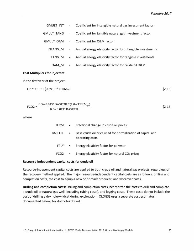
GMULT_INT = Coefficient for intangible natural gas investment factor

GMULT_TANG = Coefficient for tangible natural gas investment factor

GMULT_OAM = Coefficient for O&M factor

INTANG_M = Annual energy elasticity factor for intangible investments

TANG_M = Annual energy elasticity factor for tangible investments

OAM_M = Annual energy elasticity factor for crude oil O&M

Cost Multipliers for Injectant:

In the first year of the project:

FPLY = 1.0 + (0.3913 * TERMiyr) (2-15)

FCO2 = BASEOIL*0.0130.5

)TERM(1.0*BASEOIL*0.0130.5 iyr

(2-16)

where

TERM = Fractional change in crude oil prices

BASEOIL = Base crude oil price used for normalization of capital and

operating costs

FPLY = Energy elasticity factor for polymer

FCO2 = Energy elasticity factor for natural CO2 prices

Resource-Independent capital costs for crude oil

Resource-independent capital costs are applied to both crude oil and natural gas projects, regardless of

the recovery method applied. The major resource-independent capital costs are as follows: drilling and

completion costs, the cost to equip a new or primary producer, and workover costs.

Drilling and completion costs: Drilling and completion costs incorporate the costs to drill and complete

a crude oil or natural gas well (including tubing costs), and logging costs. These costs do not include the

cost of drilling a dry hole/wildcat during exploration. OLOGSS uses a separate cost estimator,

documented below, for dry holes drilled.

February 2017


Drilling and completion costs:

DWC_Wr = DNCC_COEF1,1,r * exp(-DNCC_COEF1,2,r * DEPTH)

+ DNCC_COEF1,3,r * (DEPTH + NLAT*LATLEN) + DNCC_COEF1,4,r * (DEPTH + NLAT*LATLEN)2

+ DNCC_COEF1,5,r * exp(DNCC_COEF1,6,r * DEPTH) (2-17)

where

DWC_W = Cost to drill and complete a crude oil well (K$/Well)

r = Region number

DNCC_COEF = Coefficients for drilling cost equation

DEPTH = Well depth (feet)

NLAT = Number of laterals

LATLEN = Length of lateral (feet)

Drilling costs for a dry well:

DRY_Wr = DNCC_COEF3,1,r * exp(-DNCC_COEF3,2,r * DEPTH)



where

DRY_W = Cost to drill a dry well (K$/Well)

r = Region number

DNCC_COEF = Coefficients for dry well drilling cost equation

DEPTH = Well depth


LATLEN = Length of lateral (feet)

Cost to equip a new producer: The cost of equipping a primary producing well includes the production

equipment costs for primary recovery.

NPR_Wr,d = NPRKr, d + (NPRAr, d * DEPTH) + (NPRBr, d * DEPTH2)

+ (NPRCr, d * DEPTH3) (2-19)

February 2017


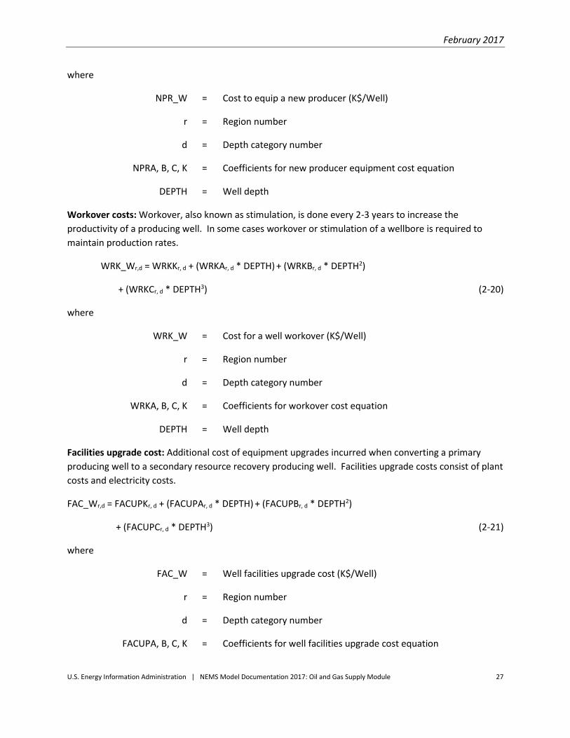
where

NPR_W = Cost to equip a new producer (K$/Well)

r = Region number

d = Depth category number

NPRA, B, C, K = Coefficients for new producer equipment cost equation

DEPTH = Well depth

Workover costs: Workover, also known as stimulation, is done every 2-3 years to increase the

productivity of a producing well. In some cases workover or stimulation of a wellbore is required to

maintain production rates.

WRK_Wr,d = WRKKr, d + (WRKAr, d * DEPTH) + (WRKBr, d * DEPTH2)

+ (WRKCr, d * DEPTH3) (2-20)

where

WRK_W = Cost for a well workover (K$/Well)

r = Region number


WRKA, B, C, K = Coefficients for workover cost equation

DEPTH = Well depth

Facilities upgrade cost: Additional cost of equipment upgrades incurred when converting a primary

producing well to a secondary resource recovery producing well. Facilities upgrade costs consist of plant

costs and electricity costs.

FAC_Wr,d = FACUPKr, d + (FACUPAr, d * DEPTH) + (FACUPBr, d * DEPTH2)

+ (FACUPCr, d * DEPTH3) (2-21)

where

FAC_W = Well facilities upgrade cost (K$/Well)

r = Region number


FACUPA, B, C, K = Coefficients for well facilities upgrade cost equation

February 2017


DEPTH = Well depth

Resource-independent capital costs for natural gas

Drilling and completion costs: Drilling and completion costs incorporate the costs to drill and complete

a crude oil or natural gas well (including tubing costs), and logging costs. These costs do not include the

cost of drilling a dry hole/wildcat during exploration. OLOGSS uses a separate cost estimator,

documented below, for dry holes drilled. Vertical well drilling costs include drilling and completion of

vertical, tubing, and logging costs. Horizontal well costs include costs for drilling and completing a

vertical well and the horizontal laterals.

Drilling and completion costs:

DWC_Wr = DNCC_COEF2,1,r * exp(-DNCC_COEF2,2,r * DEPTH)



where

DWC_W = Cost to drill and complete a natural gas well (K$/Well)

r = Region number

DNCC_COEF = Coefficients for drilling cost equation

DEPTH = Well depth


LATLEN = Length of lateral

Drilling costs for a dry well:

DRY_Wr = DNCC_COEF3,1,r * exp(-DNCC_COEF3,2,r * DEPTH)



where

DRY_W = Cost to drill a dry well (K$/Well)

r = Region number

DNCC_COEF = Coefficients for dry well drilling cost equation

February 2017


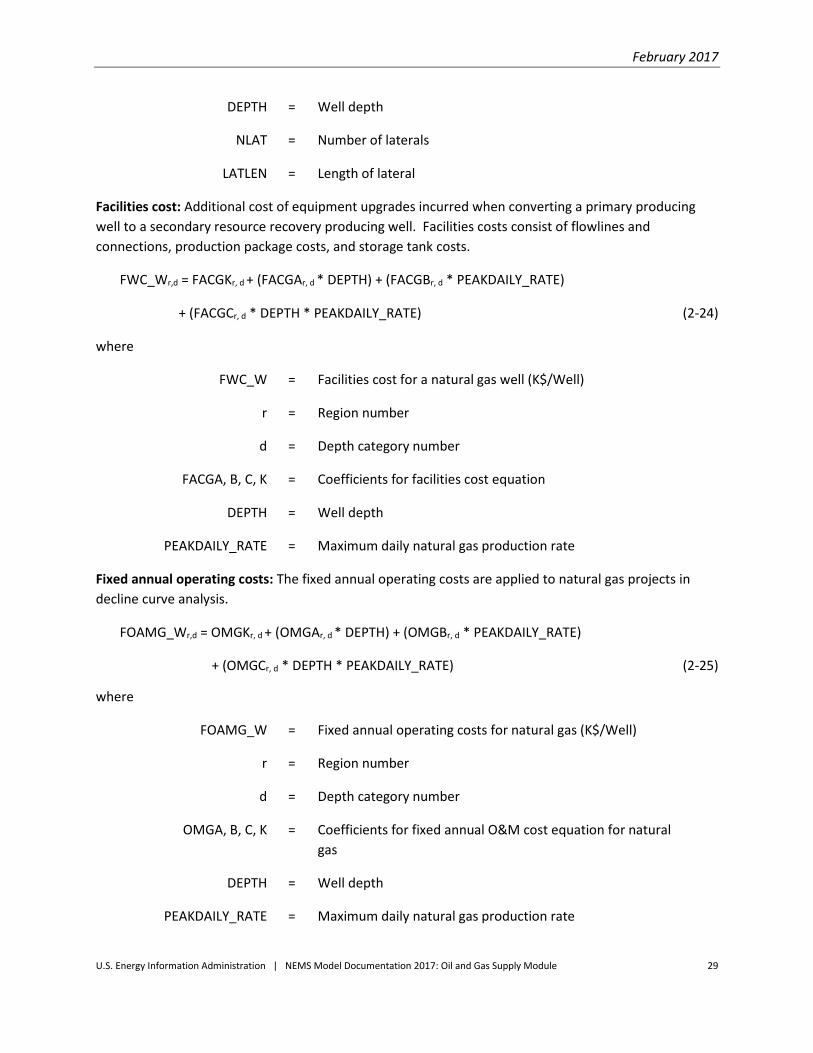
DEPTH = Well depth


LATLEN = Length of lateral

Facilities cost: Additional cost of equipment upgrades incurred when converting a primary producing

well to a secondary resource recovery producing well. Facilities costs consist of flowlines and

connections, production package costs, and storage tank costs.

FWC_Wr,d = FACGKr, d + (FACGAr, d * DEPTH) + (FACGBr, d * PEAKDAILY_RATE)

+ (FACGCr, d * DEPTH * PEAKDAILY_RATE) (2-24)

where

FWC_W = Facilities cost for a natural gas well (K$/Well)

r = Region number


FACGA, B, C, K = Coefficients for facilities cost equation

DEPTH = Well depth

PEAKDAILY_RATE = Maximum daily natural gas production rate

Fixed annual operating costs: The fixed annual operating costs are applied to natural gas projects in

decline curve analysis.

FOAMG_Wr,d = OMGKr, d + (OMGAr, d * DEPTH) + (OMGBr, d * PEAKDAILY_RATE)

+ (OMGCr, d * DEPTH * PEAKDAILY_RATE) (2-25)

where

FOAMG_W = Fixed annual operating costs for natural gas (K$/Well)

r = Region number


OMGA, B, C, K = Coefficients for fixed annual O&M cost equation for natural

gas

DEPTH = Well depth

PEAKDAILY_RATE = Maximum daily natural gas production rate

February 2017


Resource-independent annual operating costs for crude oil

Fixed Operating Costs: The fixed annual operating costs are applied to crude oil projects in decline curve

analysis.

OMO_Wr,d = OMOKr, d + (OMOAr, d * DEPTH) + (OMOBr, d * DEPTH2)

+ (OMOCr, d * DEPTH3) (2-26)

where

OMO_W = Fixed annual operating costs for crude oil wells (K$/Well)

r = Region number


OMOA, B, C, K = Coefficients for fixed annual operating cost equation for

crude oil

DEPTH = Well depth

Annual costs for secondary producers: The direct annual operating expenses include costs in the

following major areas: normal daily expenses, surface maintenance, and subsurface maintenance.

OPSEC_Wr,d = OPSECKr, d + (OPSECAr, d * DEPTH) + (OPSECBr, d * DEPTH2)

+ (OPSECCr, d * DEPTH3) (2-27)

where

OPSEC_W = Fixed annual operating cost for secondary oil operations

(K$/Well)

r = Region number


OPSECA, B, C, K = Coefficients for fixed annual operating cost for secondary oil

operations

DEPTH = Well depth

Lifting costs: Incremental costs are added to a primary and secondary flowing well. These costs include

pump operating costs, remedial services, workover rig services and associated labor.

OML_Wr,d = OMLKr, d + (OMLAr, d * DEPTH) + (OMLBr, d * DEPTH2)

+ (OMLCr, d * DEPTH3) (2-28)

February 2017


where

OML_W = Variable annual operating cost for lifting (K$/Well)

r = Region number


OMLA, B, C, K = Coefficients for variable annual operating cost for lifting

equation

DEPTH = Well depth

Secondary workover: Secondary workover, also known as stimulation, is done every 2-3 years to increase the productivity of a secondary producing well. In some cases secondary workover or stimulation of a wellbore is required to maintain production rates.

SWK_Wr,d = OMSWRKr, d + (OMSWR Ar, d * DEPTH) + (OMSWR Br, d * DEPTH2)

+ (OMSWR Cr, d * DEPTH3) (2-29)

where

SWK_W = Secondary workover costs (K$/Well)

r = Region number


OMSWRA, B, C, K = Coefficients for secondary workover costs equation

DEPTH = Well depth

Stimulation costs: Workover, also known as stimulation, is done every 2-3 years to increase the

productivity of a producing well. In some cases workover or stimulation of a wellbore is required to

maintain production rates.

STIM_W =

1000

DEPTH*STIM_BSTIM_A (2-30)

where

STIM_W = Oil stimulation costs (K$/Well)

STIM_A, B = Stimulation cost equation coefficients

DEPTH = Well depth

February 2017


Resource-dependent capital costs for crude oil

Cost to convert a primary well to a secondary well: These costs consist of additional costs to equip a

primary producing well for secondary recovery. The cost of replacing the old producing well equipment

includes costs for drilling and equipping water supply wells but excludes tubing costs.

PSW_Wr,d = PSWKr, d + (PSWAr, d * DEPTH) + (PSWBr, d * DEPTH2)

+ (PSWCr, d * DEPTH3) (2-31)

where

PSW_W = Cost to convert a primary well into a secondary well

(K$/Well)

r = Region number


PSWA, B, C, K = Coefficients for primary to secondary well conversion cost

equation

DEPTH = Well depth

Cost to convert a producer to an injector: Producing wells may be converted to injection service

because of pattern selection and favorable cost comparison against drilling a new well. The conversion

procedure consists of removing surface and sub-surface equipment (including tubing), acidizing and

cleaning out the wellbore, and installing new 2⅞-inch plastic-coated tubing and a waterflood packer

(plastic-coated internally and externally).

PSI_Wr,d = PSIKr, d + (PSIAr, d * DEPTH) + (PSIBr, d * DEPTH2)

+ (PSICr, d * DEPTH3) (2-32)

where

PSI_W = Cost to convert a producing well into an injecting well

(K$/Well)

r = Region number

D = Depth category number

PSIA, B, C, K = Coefficients for producing to injecting well conversion cost

equation

DEPTH = Well depth

February 2017


Cost of produced water handling plant: The capacity of the water treatment plant is a function of the

maximum daily rate of water injected and produced (Mbbl) throughout the life of the project.

PWP_F =

365

RMAXW*PWHP (2-33)

where

PWP_F = Cost of the produced water handling plant (K$/Well)

PWHP = Produced water handling plant multiplier

RMAXW = Maximum pattern level annual water injection rate

Cost of chemical handling plant (non-polymer): The capacity of the chemical handling plant is a function

of the maximum daily rate of chemicals injected throughout the life of the project.

CHM_F =

CHMB

365

RMAXP*CHMA*CHMK

(2-34)

where

CHM_F = Cost of chemical handling plant (K$/Well)

CHMB = Coefficient for chemical handling plant cost equation

CHMK, A = Coefficients for chemical handling plant cost equation

RMAXP = Maximum pattern level annual polymer injection rate

Cost of polymer handling plant: The capacity of the polymer handling plant is a function of the

maximum daily rate of polymer injected throughout the life of the project.

PLY_F =

6.0

365

RMAXP*PLYPA*PLYPK

(2-35)

where

PLY_F = Cost of polymer handling plant (K$/Well)

PLYPK, A = Coefficients for polymer handling plant cost equation

RMAXP = Maximum pattern level annual polymer injection rate

February 2017


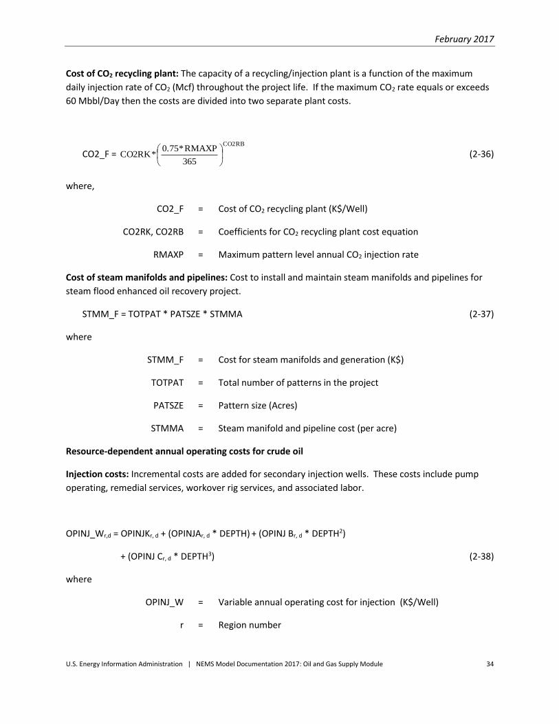
Cost of CO2 recycling plant: The capacity of a recycling/injection plant is a function of the maximum

daily injection rate of CO2 (Mcf) throughout the project life. If the maximum CO2 rate equals or exceeds

60 Mbbl/Day then the costs are divided into two separate plant costs.

CO2_F = CO2RB

365

RMAXP*0.75*CO2RK

(2-36)

where,

CO2_F = Cost of CO2 recycling plant (K$/Well)

CO2RK, CO2RB = Coefficients for CO2 recycling plant cost equation

RMAXP = Maximum pattern level annual CO2 injection rate

Cost of steam manifolds and pipelines: Cost to install and maintain steam manifolds and pipelines for

steam flood enhanced oil recovery project.

STMM_F = TOTPAT * PATSZE * STMMA (2-37)

where

STMM_F = Cost for steam manifolds and generation (K$)

TOTPAT = Total number of patterns in the project

PATSZE = Pattern size (Acres)

STMMA = Steam manifold and pipeline cost (per acre)

Resource-dependent annual operating costs for crude oil

Injection costs: Incremental costs are added for secondary injection wells. These costs include pump

operating, remedial services, workover rig services, and associated labor.

OPINJ_Wr,d = OPINJKr, d + (OPINJAr, d * DEPTH) + (OPINJ Br, d * DEPTH2)

+ (OPINJ Cr, d * DEPTH3) (2-38)

where

OPINJ_W = Variable annual operating cost for injection (K$/Well)

r = Region number

February 2017



OPINJA, B, C, K = Coefficients for variable annual operating cost for injection

equation

DEPTH = Well depth

Injectant cost: The injectant costs are added for the secondary injection wells. These costs are specific

to the recovery method selected for the project. Three injectants are modeled: polymer, CO2 from

natural sources, and CO2 from industrial sources.

Polymer cost:

POLYCOST = POLYCOST * FPLY (2-39)

where

POLYCOST = Cost of polymer ($/Lb)

FPLY = Energy elasticity factor for polymer

Natural CO2 cost: Cost to drill, produce and ship CO2 from natural sources, namely CO2 fields in Western

Texas.

CO2COST = (CO2K + (CO2B * OILPRICEO(1))) * CO2PR(IST) (2-40)

where

CO2COST = Cost of natural CO2 ($/Mcf)

IST = State identifier

CO2K, CO2B = Coefficients for natural CO2 cost equation

OILPRICEO(1) = Crude oil price for first year of project analysis

CO2PR = State CO2 cost multiplier used to represent changes in cost

associated with transportation outside of the Permian Basin

Industrial CO2 cost: Cost to capture and transport CO2 from industrial sources. These costs include the

capture, compression to pipeline pressure, and the transportation to the project site via pipeline.

Industrial CO2 sources include

Hydrogen Plants

Ammonia Plants

Ethanol Plants

February 2017


Cement Plants

Hydrogen Refineries

Power Plants

Natural Gas Processing Plants

Coal-to-Liquids Plants

The regional costs, which are specific to the industrial source of CO2, are exogenously determined and

provided in the input file, except for power plants and coal-to-liquids plants. After unit costs have been

calculated for the project, they are adjusted using technology levers as well as CPI multipliers. Two

types of levers are applied to the costs. The first is the fractional change in cost associated with a new

technology. The second is the incremental cost associated with implementing the new technology.

These factors are determined by the model user. As an example,

NPR_W = (UNPR_W * CHG_FAC_FAC(ITECH)) + CST_FAC_FAC(ITECH) (2-41)

where

NPR_W

UNPR_W

=

=

Cost to equip a new oil producer (K$/well)

Cost to equip a new oil producer before technology

adjustments (K$/well)

CHG_FAC_FAC = Fractional change in cost associated with technology

improvements

CST_FAC_FAC = Incremental cost to apply the new technology

ITECH = Technology case (Base or Advanced)

The costs for CO2 from power plants and coal-to-liquids plants are determined in the Capture, Transport,

Utilization, and Storage (CTUS) Submodule and passed to OGSM (see Appendix 2.D for the description of

the integration with the CTUS Submodel).

Determining technical production

The development schedule algorithms determine how the project’s development over time will be

modeled. They calculate the number of wells initiated per year and the economic life of the well. The

economic life is the number of years in which the revenue from production exceeds the costs required

to produce the crude oil and natural gas.

The model then aggregates the well-level production of crude oil, natural gas, water, and injectant

based upon the well life and number of wells initiated each year. The resulting profile is the technical

production for the project.

February 2017


Figure 2-8 shows the crude oil production for one hypothetical project over the course of its life. In this

scenario new wells are drilled for five years. Each shaded area is the annual technical production

associated with the active wells by vintage year.

Figure 2-8. Calculating project-level technical production

The first step in modeling the technical production is to calculate the number of wells drilled each year.

The model uses several factors in calculating the development schedule:

Potential delays between the discovery of the project and actual initiation

The process modeled

The resource access – the number of wells developed each year is reduced if the resource is

subject to cumulative surface use limitations

The total number of wells needed to develop the project

The crude oil and natural gas prices

Expected production rate in first year to allow highgrading – for example, drilling is reduced

more in low productivity areas than in high productivity areas when prices decrease

The user-specified maximum and minimum number of wells developed each year

The user-specified percentage of the project to be developed each year

The percentage of the project which is using base or advanced technology

After calculating the number of wells drilled each year, the model calculates the number of wells which

are active (producing) for each year of the project life.

February 2017


Crude Oil and Natural Gas Production Profile of the Project: For all EOR/ASR, undiscovered, and

developing processes, the project-level technical production is calculated using well-level production

profiles—the sum of the well-level production for each profile give the estimated ultimate recovery per

well (EUR). For infill projects, the production is doubled because the model assumes that there are two

producers in each pattern. These profiles change over the projection period depending on the assumed

impact of technological progress (increases the expected per well production rate, see technology

section on page 66) and diminishing returns as horizontal tight and shale wells are drilled closer together

(the productivity of each new well eventually is reduced as they start to interfere with each other). The

impact of diminishing returns is realized when the spacing of wells drops below 100 acres and is

represented by

adjusted_prod_profilet = orig_prod_profilet ∗ (1.0 − 0.1 ∗100

wlspcyear) (2-42)

where

adjusted_prod_profile = Revised production profile for tight/shale oil and natural gas

wells that are drilled in areas with less than 100 acre well

spacing

orig_prod_profile = Original production profile for tight/shale oil and natural gas

wells

wlspc = Wells spacing (acres)

t Normalized year of production (first year (1) - last year (30))

year = Projection year (2016-2050)

Crude Type: Production from each play/sub-play has an assumed average API gravity (degrees) and

sulfur content (percent). Crude oil production (including lease condensates) is grouped into the

following crude type categories:

1) Light sweet: 35 ≤ API < 40, sulfur < 0.5

2) Light sour: API≥ 35, sulfur ≥ 0.5

3) Medium medium sour: 27 ≤ API <35, sulfur < 1.1

4) Medium sour: 27 ≤ API <35, sulfur ≥ 1.1

5) Heavy sweet: API < 27, sulfur < 1.1

6) Heavy sour: API < 27, sulfur ≥ 1.1

7) California: all API and sulfur

8) Syncrude: not U.S.

9) DilBit/SynBit: not U.S.

10) Ultra light sweet: 40 ≤ API < 50, sulfur < 0.5

11) 50+ sweet: API≥ 50, sulfur < 0.5

February 2017


Natural gas plant liquids production: The revenue generated from the production of natural gas plant

liquids (NGPLs) is included in the economic evaluation of the project. NGPLs are determined by applying

a play-level factor (in barrels per million cubic feet) to the well-level natural gas production profile. The

price applied to the NGPL volumes is the industrial LPG feedstock price determined in the LFMM. The

composition of NGPL production is determined using assumed shares of ethane, propane, butane,

isobutene, and pentanes plus.

Resource accounting

OLOGSS incorporates a complete and representative description of the processes by which crude oil and

natural gas in the technically recoverable resource base are converted to proved reserves.

OLOGSS distinguishes between drilling for new fields (new field wildcats) and drilling for additional

deposits within old fields (other exploratory and developmental wells). This enhancement recognizes

important differences in exploratory drilling, both by its nature and in its physical and economic returns.

New field wildcats convert resources in previously undiscovered fields4 into both proved reserves (as

new discoveries) and inferred reserves.5 Other exploratory drilling and developmental drilling add to

proved reserves from the stock of inferred reserves. The phenomenon of reserves appreciation is the

process by which initial assessments of proved reserves from a new field discovery grow over time

through extensions and revisions.

End-of-year reserves: Proved reserves are calculated as the technical production from wells initiated

through a particular year minus the cumulative production from those wells.

Calculating project costs

The model uses four drilling categories for the calculation of drilling and facilities costs. These

categories are:

New producers

New injectors

Conversions of producers to injectors

Conversions of primary wells to secondary wells

The number of wells in each category is dependent upon the process and the project.

Project-level process-independent costs

Drilling costs and facility costs are determined at the project level.

4 Undiscovered resources are located outside of oil and gas fields, in which the presence of resources has been confirmed by

exploratory drilling, and thus exclude reserves and reserve extensions; however, they include resources from undiscovered

pools within confirmed fields to the extent that such resources occur as unrelated accumulations controlled by distinctly

separate structural features or stratigraphic conditions. 5 Inferred reserves are that part of expected ultimate recovery from known fields in excess of cumulative production plus

current reserves.

February 2017


Drilling costs: Drilling costs are calculated using one of four approaches, depending on the resource and

recovery process. These approaches apply to the following resources:

Undiscovered crude oil and natural gas

Existing crude oil and natural gas fields

EOR/ASR projects

Developing natural gas projects

For undiscovered crude oil and natural gas resources: The first well drilled in the first year of the project

is assumed to be a wildcat well. The remaining wells are assumed to be undiscovered development

wells. This is reflected in the application of the dryhole rates.

DRL_CST2iyr = (DWC_W* PATNiyr + DRY_W*REGDRYUER +

DRY_W*REGDRYUDR*(PATNiyr – 1)) * XPP1 (2-43)

For existing crude oil and natural gas fields: As the field is already established, the developmental

dryhole rate is used.

DRL_CST2iyr = (DWC_W + DRY_W * REGDRYKDR) * (PATDEVires,iyr, itech * XPP1) (2-44)

For EOR/ASR projects: As the project is in an established and known field, the developmental dryhole

rate is used.

DRL_CST2iyr = (DWC_W + DRY_W * REGDRYKDr) * (PATNiyr * XPP1) (2-45)

For developing natural gas projects: As the project is currently being developed, it is assumed that the

wildcat well(s) have previously been drilled. Therefore, the undiscovered developmental dryhole rate is

applied to the project.

DRL_CST2iyr = (DWC_W + DRY_W * REGDRYUDr) * (PATNiyr * XPP1) (2-46)

where

ires = Project index number

iyr = Year

R = Region

PATDEV = Number of wells drilled each year for base and advanced

technology cases

PATN = Annual number of wells drilled

DRL_CST2 = Technology-case-specific annual drilling cost

DWC_W = Cost to drill and complete a well

February 2017


DRY_W = Cost to drill a dry hole

REGDRYUE = Dryhole rate for undiscovered exploration (wildcat)

REGDRYUD = Dryhole rate for undiscovered development

REGDRYKD = Dryhole rate for known fields development

XPP1 = Number of producing wells drilled per pattern

Facilities costs: Facilities costs depend on both the process and the resource. Five approaches are used

to calculate the facilities costs for the project.

For undiscovered and developing natural gas projects:

FACCOSTiyr = (FWC_W * PATNiyr * XPP1) (2-47)

For existing natural gas fields:

FACCOSTiyr = (FWC_W * (PATDEVires,iyr, itech) * XPP1) (2-48)

For undiscovered continuous crude oil:

FACCOSTiyr = (NPR_W * PATNiyr * XPP1) (2-49)

For existing crude oil fields:

FACCOSTiyr = (PSW_W * (PATDEVires,iyr, itech) * XPP4) (2-50)

+ (PSI_W * PATDEVires,iyr, itech * XPP3)

+ (FAC_W * PATDEVires,iyr, itech * (XPP1 + XPP2))

For undiscovered conventional crude oil and EOR/ASR projects:

FACCOSTiyr = (PSW_W * PATNiyr *XPP4) (2-51)

+ (PSI_W * PATNiyr * XPP3) + (FAC_W * PATNiyr * (XPP1 + XPP2))

where

iyr = Year

ires = Project index number

itech = Technology case

PATN = Number of patterns initiated each year for the technology

case being evaluated

February 2017


PATDEV = Number of patterns initiated each year for base and

advanced technology cases

XPP1 = Number of new production wells drilled per pattern

XPP2 = Number of new injection wells drilled per pattern

XPP3 = Number of producers converted to injectors per pattern

XPP4 = Number of primary wells converted to secondary wells per

pattern

FAC_W = Crude oil well facilities upgrade cost

NPR_W = Cost to equip a new producer

PSW_W = Cost to convert a primary well to a secondary well

PSI_W = Cost to convert a production well to an injection well

FWC_W = Natural gas well facilities cost

FACCOST = Annual facilities cost for the well

February 2017


Injectant cost added to operating and maintenance: The cost of injectant is calculated and added to

the operating and maintenance costs.

INJiyr = INJ_OAM1 * WATINJiyr (2-52)

where

iyr = Year

INJ = Annual injection cost

INJ_OAM1 = Process-specific cost of injection ($/bbl)

WATINJ = Annual project level water injection

For infill drilling: Injectant costs are zero.

Fixed annual operating costs for crude oil:

For CO2 EOR:

AOAMiyr = OPSEC_W * SUMPiyr (2-53)

For undiscovered conventional crude oil:

Fixed annual operating costs for secondary oil wells are assumed to be zero.

For all crude oil processes except CO2 EOR:

AOAMiyr = (OMO_W * XPATNiyr) + (OPSEC_W * XPATNiyr) (2-54)

Fixed annual operating costs for natural gas:

For existing natural gas fields:

AOAMiyr = (FOAMG_W * OAM_Miyr * XPATNiyr) (2-55)

For undiscovered and developing natural gas resources:

AOAMiyr = (FOAMG_W * OAM_Miyr * XPATNiyr) * XPP1 (2-56)

where

AOAM = Annual fixed operating and maintenance costs

iyr = Year

SUMP = Total cumulative patterns initiated

OPSEC_W = Fixed annual operating costs for secondary oil wells

February 2017


OMO_W = Fixed annual operating costs for crude oil wells

FOAMG_W = Fixed annual operating costs for natural gas wells

OAM_M = Energy elasticity factor for operating and maintenance costs

XPATN = Annual number of active patterns


Variable operating costs:

OAMiyr = (OILPRODiyr* OIL_OAM1 + GASPRODiyr* GAS_OAM1 +

WATPRODiyr* WAT_OAM1) * OAM_Miyr + INJiyr

STIMiyr = STIMiyr + (0.2 * STIM_W * XPATNiyr * XPP1) (2-57)

where

OAM = Annual variable operating and maintenance costs

OILPROD = Annual project-level crude oil production

GASPROD = Annual project-level natural gas production

WATPROD = Annual project-level water injection

OIL_OAM1 = Process-specific cost of crude oil production ($/bbl)

GAS_OAM1 = Process-specific cost of natural gas production ($/Mcf)

WAT_OAM1 = Process-specific cost of water production ($/bbl)


STIM = Project stimulation costs

STIM_W = Well stimulation costs

INJ = Cost of injection

XPATN = Annual number of active patterns

iyr = Year


February 2017


Cost of compression (natural gas processes):

Installation costs:

COMPiyr = COMPiyr + (COMP_W*PATNiyr*XPP1) (2-58)

O&M cost for compression:

OAM_COMPiyr = OAM_COMPIYR + (GASPRODiyr * COMP_OAM

*OAM_Miyr) (2-59)

COMP = Cost of installing natural gas compression equipment

COMP_W = Natural gas compression cost

PATN = Number of patterns initiated each year

iyr = Year


OAM_COMP = Operating and maintenance costs for natural gas compression


COMP_OAM = Compressor O&M costs

OAM_M = Energy elasticity factor for O&M costs

Process-dependent costs

Process-specific facilities and capital costs are calculated at the project level.

Facilities costs

Profile model: The facilities cost of a water handling plant is added to the first year facilities costs.

FACCOST1 =

365

RMAX*PWHPFACCOST1

(2-60)

where

FACCOST1 = First year of project facilities costs

PWHP = Produced water handling plant multiplier

RMAX = Maximum annual water injection rate

February 2017


Polymer model: The facilities cost for a water handling plant is added to the first year facilities costs.

FACCOST1 = FACCOST1 + PWP_F (2-61)

where

FACCOST1 = First year of project facilities costs

PWP_F = Produced water handling plant cost

Advanced CO2: Other costs added to the facilities costs include the facilities cost for a CO2 handling plant

and a recycling plant, the O&M (fixed and variable) cost for a CO2 handling plant and recycling plant, and

injectant cost. If the plant is developed in a single stage, the costs are added to the first year of the

facilities costs. If a second stage is required, the additional costs are added to the sixth year of facilities

costs.

FACCOST1 = FACCOST1 + 000,1*365

RMAX*0.75*CO2RK

CO2RB

(2-62)

FACCOST6 = FACCOST6 + 000,1*365

RMAX*0.75*CO2RK

CO2RB

INJiyr = INJiyr + (TOTINJiyr – TORECYiyr) * CO2COST (2-63)

OAMiyr = OAMiyr + (OAM_Miyr * TORECYiyr) *

(CO2OAM + PSW_W * 0.25) (2-64)

FOAMiyr = (FOAMiyr + TOTINJiyr) * 0.40 * FCO2 (2-65)

TORECY_CSTiyr = TORECY_CSTiyr + (TORECYiyr * CO2OAM2 * OAM_Miyr) (2-66)

where

iyr = Year

RMAX = Maximum annual volume of recycled CO2

CO2OAM = O&M cost for CO2 handling plant

CO2OAM2 = The O&M cost for the project’s CO2 injection plant

CO2RK, CO2RB = CO2 recycling plant cost coefficients

PSW_W = Cost to convert a primary well to a secondary well

INJ = Cost of purchased CO2

February 2017


TOTINJ = Annual project-level volume of injected CO2

TORECY = Annual project-level CO2 recycled volume

CO2COST = Cost of CO2 ($/mcf)

OAM = Annual variable O&M costs


FOAM = Fixed annual operating and maintenance costs

FCO2 = Energy elasticity factor for CO2

FACCOST = Annual project facilities costs

TORECY_CST = The annual cost of operating the CO2 recycling plant

Steam model: Facilities and O&M costs for steam generators and recycling.

Recalculate the facilities costs: Facilities costs include the capital cost for injection plants, which is

based upon the original oil in place (OOIP) of the project, the steam recycling plant, and the steam

generators required for the project.

FACCOST1 = FACCOST1 +

TOTPAT

APATOOIP *0.2*1.0*+ (RECY_WAT * RMAXWAT

+ RECY_OIL * RMAXOIL) + (STMMA * TOTPAT * PATSIZE)

+ (IGENiyr – IG )* STMGA (2-67)

OAMiyr = OAMiyr + (WAT_OAM1 * WATPRODiyr * OAM_Miyr) + (OIL_OAM1

* OILPRODiyr * OAM_Miyr) + (INJ_OAM1 * WATINJiyr * OAM_Miyr) (2-68)

where

iyr = Year

IGEN = Number of active steam generators each year

IG = Number of active steam generators in previous year

FACCOST = Annual project level facilities costs

RMAXWAT = Maximum daily water production rate

February 2017


RMAXOIL = Maximum daily crude oil production rate

APAT = Number of developed patterns

TOTPAT = Total number of patterns in the project

OOIP = Original oil in place (MMbbl)

PATSIZE = Pattern size (acres)

STMMA = Unit cost for steam manifolds

STMGA = Unit cost for steam generators

OAM = Annual variable operating and maintenance costs




INJ_OAM1 = Process-specific cost of water injection ($/bbl)

OILPROD = Annual project level crude oil production

WATPROD = Annual project level water production

WATINJ = Annual project level water injection

RECY_WAT = Recycling plant cost – water factor

RECY_OIL = Recycling plant cost – oil factor

Operating and maintenance cost

This subroutine calculates the process-specific O&M costs.

Profile model: Add the O&M costs of injected polymer.

INJiyr = 1000

POLYCOST* TOTINJ * OAM_MINJ

iyriyriyr (2-69)

OAMiyr = OAMiyr + (XPATNiyr * 0.25 * PSI_W) (2-70)

February 2017


where

iyr = Year

INJ = Annual injection cost

OAM_M = Energy elasticity factor for operating and maintenance cost

TOTINJ = Annual project-level injectant injection volume

POLYCOST = Polymer cost

OAM = Annual variable operating and maintenance cost

XPATN = Number of active patterns

PSI_W = Cost to convert a primary well to an injection well

Polymer: Add the O&M costs of injected polymer.

INJiyr = 1,000

POLYCOST*TOTINJINJ

iyr

IYR (2-71)


where

IYR = Year

INJ = Annual Injection cost

TOTINJ = Annual project-level injectant injection volume

POLYCOST = Polymer cost

OAM = Annual variable O&M cost



Waterflood: Add the O&M cost to convert a primary well to an injection well.


February 2017


where

iyr = Year

OAM = Annual variable O&M cost



Existing crude oil fields and reservoirs: Since no new drilling or major investments are expected for

reservoirs in decline, facilities and drilling costs are zeroed out.

OAMiyr = OAMiyr + ((OIL_OAM1 * OILPRODiyr) + (GAS_OAM1 * GASPRODiyr)

+ (WAT_OAM1 * WATPRODiyr)) * OAM_Miyr (2-74)

AOAMiyr = AOAMiyr +

5

SUMP*OAM_M*OPSEC_W iyriyr (2-75)

where

iyr = Year

OILPROD = Annual project-level crude oil production


WATPROD = Annual project-level water production


GAS_OAM1 = Process-specific cost of natural gas production ($/Mcf)



OPSEC_W = Fixed annual operating cost for secondary well operations

SUMP = Cumulative patterns developed

AOAM = Fixed annual O&M costs

OAM = Variable annual O&M costs

February 2017


Overhead costs: : General and Administrative (G&A) costs on capitalized and expensed items, which

consist of administration, accounting, contracting and legal fees/expenses for the project, are calculated

according to the following equations:

GNA_EXPitech = GNA_EXPitech * CHG_GNA_FACitech (2-76)

GNA_CAPitech = GNA_CAPitech * CHG_GNA_FACitech (2-77)

where

itech = Technology case (base and advanced) number

GNA_EXP = The G&A rate applied to expensed items for the project

GNA_CAP = The G&A rate applied to capitalized items for the project

CHG_GNA_FAC = Technology-case-specific change in G&A rates

Timing

Overview of timing module

The timing routine determines which of the exploration and EOR/ASR projects are eligible for

development in any particular year. Those that are eligible are subject to an economic analysis and

passed to the project sort and development routines. The timing routine has two sections. The first

applies to exploration projects, while the second is applied to EOR/ASR and developing natural gas

projects.

Figure 2-9 provides the overall logic for the exploration component of the timing routine. For each

project, regional crude oil and natural gas prices are obtained. The project is then examined to see if it

has previously been timed and developed. The timed projects are no longer available and thus not

considered.

The model uses four resource access categories for the undiscovered projects:

No leasing due to statutory or executive order

Leasing available but cumulative timing limitations between 3 and 9 months

Leasing available but with controlled surface use

Standard leasing terms

Each project has been assigned to a resource access category. If the access category is not available in

the year evaluated, the project fails the resource access check.

After the project is evaluated, the number of considered projects is increased. Figure 2-10 shows the

timing logic applied to the EOR/ASR projects as well as the developing natural gas projects.

Before the economics are evaluated, the prices are set and the eligibility is determined. The following

conditions must be met:

February 2017


Project has not been previously timed

Project must be eligible for timing, re-passed the economic pre-screening routine

Corresponding decline curve project must have been timed. This does not apply to the

developing natural gas projects.

If the project meets all of these criteria, then it is considered eligible for economic analysis. For an

EOR/ASR project to be considered for timing, it must be within a process-specific EOR/ASR development

window. These windows are listed in Table 2-4.

Table 2-4. EOR/ASR eligibility ranges

Process Before Economic Limit After Economic Limit

CO2 Flooding After 2009 10 Years

Steam Flooding 5 Years 10 Years

Polymer Flooding 5 Years 10 Years

Infilll Drilling After 2009 7 Years

Profile Modification 5 Years 7 Years

Horizontal Continuity 5 Years 7 Years

Horizontal Profile 5 Years 7 Years

Waterflood 4 Years 6 Years

The economic viability of the eligible projects is then evaluated. A different analytical approach is

applied to CO2 EOR and all other projects. For non-CO2 EOR projects, the project is screened for

applicable technology levers, and the economic analysis is conducted. CO2 EOR projects are treated

differently because of the different CO2 costs associated with the different sources of industrial and

natural CO2.

For each available source, the economic variables are calculated and stored. These include the source of

CO2 and the project’s ranking criterion.

Detailed description of timing module

Exploration projects: The first step in the timing module is to determine which reservoirs are eligible to

be timed for conventional and continuous exploration. Prior to evaluation, the constraints, resource

access, and technology and economic levers are checked, and the technology case is set.

Calculate economics for EOR/ASR and developing natural gas projects:

This section determines whether an EOR/ASR or developing natural gas project is eligible for economic

analysis and timing. The following resources or processes are considered in this step.

February 2017


EOR processes:

CO2 Flooding

Steam Flooding

Polymer Flooding

Profile Modification

ASR processes:

Water Flooding

Infill Drilling

Horizontal Continuity

Horizontal Profile

Developing natural gas

Tight Gas

Shale Gas

Coalbed Methane

A project is eligible for timing if the corresponding decline curve project has previously been timed and

the year of evaluation is within the eligibility window for the process, as listed in Table 2-4.

Project ranking: Sorts exploration and EOR/ASR projects which are economic and thus eligible for

timing. The subroutine matches the discovery order for undiscovered projects and sorts the others by

ranking criterion. The criteria include:

Net present value

Investment efficiency

Rate of return

Cumulative discounted after-tax cash flow

Selection and timing: Times the exploration and EOR/ASR projects which are considered in that given

year.

Project selection

The project selection subroutine determines which exploration, EOR/ASR and developing natural gas

projects will be modeled as developed in each year analyzed. In addition, the following development

decisions are made:

Waterflood of conventional undiscovered crude oil projects

Extension of CO2 floods as the total CO2 injected is increased from 0.4 hydrocarbon pore volume

(HCPV) to 1.0 HCPV

February 2017


Overview of project selection

The project selection subroutine evaluates undiscovered projects separate from other projects. The

logic for the development of exploration projects is provided in Figure 2-9.

Figure 2-9. Selecting undiscovered projects

February 2017


As illustrated in the figure, the prices are set for the project before its eligibility is checked. Eligibility has

the following requirements:

Project is economically viable

Project is not previously timed and developed

The projects which are eligible are screened for applicable technologies which impact the drilling

success rates. The development constraints required for the project are checked against those that are

available in the region.

If sufficient development resources are available, the project is timed and developed. As part of this

process, the available development constraints are adjusted, the number of available accumulations is

reduced and the results are aggregated. If no undiscovered accumulations remain, then the project is

no longer eligible for timing. The projects that are eligible, economically viable, and undeveloped due to

lack of development resources are considered again for future projection years. If the project is

conventional crude oil, it is possible to time a waterflood project.

The model evaluates the waterflood potential in a window centered upon the end of the economic life

for the undiscovered project. For each year of that window, the technical production is determined for

the waterflood project, applicable technology and economic levers are applied, and the economics are

considered. If the waterflood project is economic, it is timed. This process is continued until either a

waterflood project is timed or the window closes.

The second component of the project selection subroutine is applicable to EOR/ASR projects as well as

the developing natural gas projects. The major steps applied to these projects are detailed in Figures 2-

10 and 2-11.

As seen in the flowchart, the prices are set for the project and the eligibility is checked. As with the

undiscovered projects, the subroutine checks the candidate project for both economic viability and

eligibility for timing. Afterwards, the project is screened for any applicable technology and economic

levers.

If the project is eligible for CO2 EOR, the economics are re-run for the specific source of CO2. Afterwards,

the availability of resource development constraints is checked for the project. If sufficient drilling and

capital resources are available, the project preferences are checked.

The project preferences are rules which govern the competition between projects and selection of

projects. These rules are listed below:

CO2 EOR and infill drilling are available after 2010

Profile modification becomes available after 2011

The annual number of infill drilling and profile modification projects is limited

Horizontal continuity can compete against any other process except steam flood

Horizontal profile can compete against any other process except steam flood or profile

modification

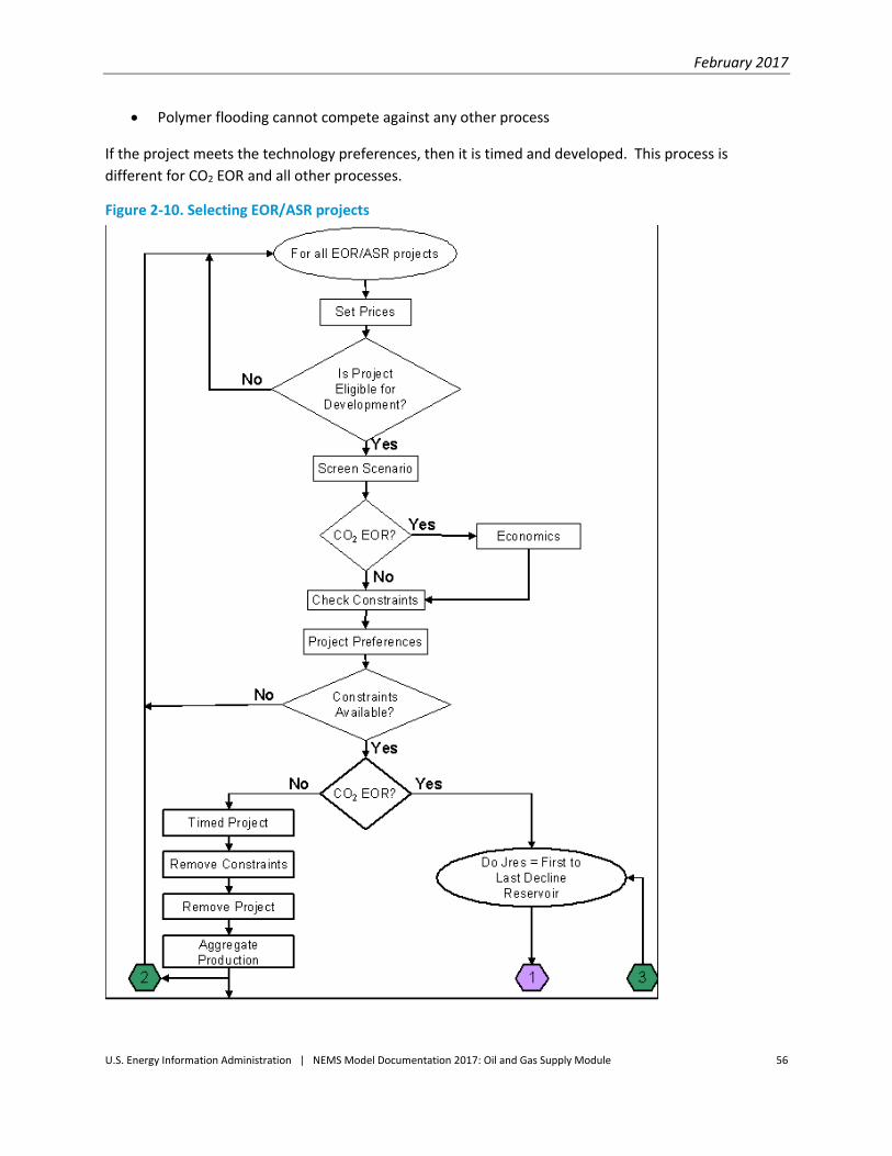
February 2017


Polymer flooding cannot compete against any other process

If the project meets the technology preferences, then it is timed and developed. This process is

different for CO2 EOR and all other processes.

Figure 2-10. Selecting EOR/ASR projects

February 2017


Figure 2-11. Selecting EOR/ASR projects

February 2017


For non-CO2 projects, the constraints are adjusted, the project is removed from the list of eligible

projects, and the results are aggregated. It is assumed that most EOR/ASR processes are mutually

exclusive and that a reservoir is limited to one process. There are a few exceptions:

CO2 EOR and infill drilling can be done in the same reservoir

CO2 EOR and horizontal continuity can be done in the same reservoir

For CO2 EOR projects, a different methodology is used at this step: the decision to increase the total CO2

injection from 0.4 hydrocarbon pore volume (HCPV) to 1.0 HCPV is made. The model performs the

following steps, illustrated in Figure 2-10 and continued in Figure 2-11.

The CO2 EOR project is matched to the corresponding decline curve project. Using the project-specific

petro-physical properties, the technical production and injection requirements are determined for the

1.0 HCPV project. After applying any applicable technology and economic levers, the model evaluates

the project economics. If the 1.0 HCPV project is not economically viable, then the 0.4 HCPV project is

timed. If the 1.0 HCPV project is viable, the constraints and project preferences are checked. Assuming

that there are sufficient development resources, and competition allows for the development of the

project, then the model times the 1.0 HCPV project. If sufficient resources for the 1.0 HCPV project are

not available, the model times the 0.4 HCPV project.

Detailed description of project selection

The project selection subroutine analyzes undiscovered crude oil and natural gas projects. If a project is

economic and eligible for development, the drilling and capital constraints are examined to determine

whether the constraints have been met. The model assumes that the projects for which development

resources are available are developed.

Waterflood processing may be considered for undiscovered conventional crude oil projects. The

waterflood project will be developed in the first year it is both eligible for implementation and

economically viable.

EOR/ASR projects

When considering whether a project is eligible for EOR/ASR processing, the model first checks for the

availability of sufficient development resources. Based on the project economics and projected

availability of development resources, it also decides whether or not to extend injection in CO2 EOR

projects from 0.4 HCPV to 1.0 HCPV.

If the 1.0 HCPV is economic but insufficient resources are available, the 0.4 HCPV project is selected

instead. If the 1.0 HCPV project is uneconomic, the 0.4 HCPV project is selected.

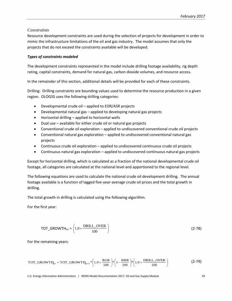
February 2017


Constraints

Resource development constraints are used during the selection of projects for development in order to

mimic the infrastructure limitations of the oil and gas industry. The model assumes that only the

projects that do not exceed the constraints available will be developed.

Types of constraints modeled

The development constraints represented in the model include drilling footage availability, rig depth

rating, capital constraints, demand for natural gas, carbon dioxide volumes, and resource access.

In the remainder of this section, additional details will be provided for each of these constraints.

Drilling: Drilling constraints are bounding values used to determine the resource production in a given

region. OLOGSS uses the following drilling categories:

Developmental crude oil – applied to EOR/ASR projects

Developmental natural gas – applied to developing natural gas projects

Horizontal drilling – applied to horizontal wells

Dual use – available for either crude oil or natural gas projects

Conventional crude oil exploration – applied to undiscovered conventional crude oil projects

Conventional natural gas exploration – applied to undiscovered conventional natural gas

projects

Continuous crude oil exploration – applied to undiscovered continuous crude oil projects

Continuous natural gas exploration – applied to undiscovered continuous natural gas projects

Except for horizontal drilling, which is calculated as a fraction of the national developmental crude oil

footage, all categories are calculated at the national level and apportioned to the regional level.

The following equations are used to calculate the national crude oil development drilling. The annual

footage available is a function of lagged five-year-average crude oil prices and the total growth in

drilling.

The total growth in drilling is calculated using the following algorithm.

For the first year:

TOT_GROWTHiyr =

100

DRILL_OVER0.1 (2-78)

For the remaining years:

100

DRILL_OVER0.1*

100

RRR1*

100

RGR1.0*TOT_GROWTHTOT_GROWTH 1-iyriyr

(2-79)

February 2017


where

iyr = Year evaluated

TOT_GROWTH = Annual growth change for drilling at the national level

(fraction)

DRILL_OVER = Percent of drilling constraint available for footage overrun

RGR = Annual rig development rate (percent)

RRR = Annual rig retirement rate (percent)

The national-level crude oil and natural gas development footage available for drilling is calculated using

the following equations. The coefficients for the drilling footage equations were estimated by least

squares using model equations 2.B-16 and 2.B-17 in Appendix 2.B.

NAT_OILiyr = (OILA0 + OILA1 * OILPRICEDIYR) * TOTMUL * TOT_GROWTHiyr

* OIL_ADJiyr (2-80)

NAT_GASiyr = (GASA0 + GASA1 * GASPRICEDIYR) * TOTMUL * TOT_GROWTHiyr

* GAS_ADJiyr (2-81)

where

iyr = Year evaluated

TOT_GROWTH = Final calculated annual growth change for drilling at the

national level

NAT_OIL NAT_GAS = National development footage available (thousand feet)

OILA0, OILA1, GASA0,

GASA1

=

Footage equation coefficients

OILPRICED, GASPRICED = Annual prices used in drilling constraints, five-year average

TOTMUL = Total drilling constraint multiplier

OIL_ADJ, GAS_ADJ = Annual crude oil, natural gas developmental drilling

availability factors

After the available footage for drilling is calculated at the national level, regional allocations are used to

allocate the drilling to each of the OLOGSS regions. The drilling which is not allocated, due to the

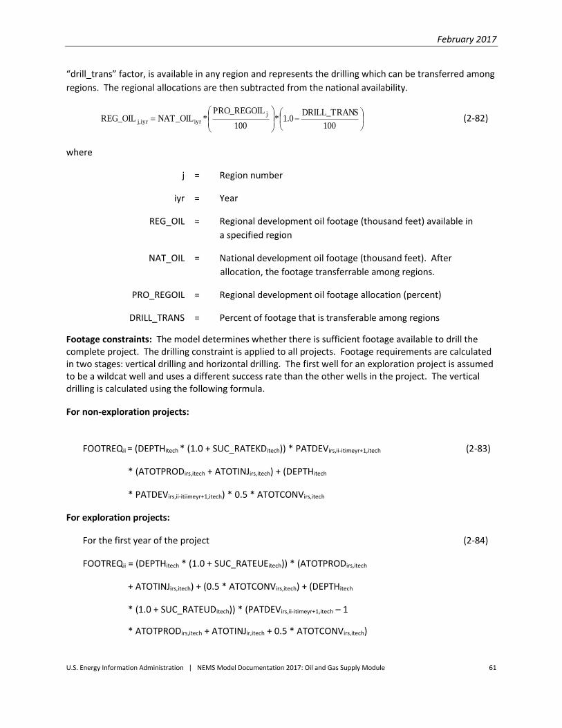
February 2017


“drill_trans” factor, is available in any region and represents the drilling which can be transferred among

regions. The regional allocations are then subtracted from the national availability.

100

SDRILL_TRAN0.1*

100

PRO_REGOIL*NAT_OILREG_OIL

j

iyriyrj, (2-82)

where

j = Region number

iyr = Year

REG_OIL = Regional development oil footage (thousand feet) available in

a specified region

NAT_OIL = National development oil footage (thousand feet). After

allocation, the footage transferrable among regions.

PRO_REGOIL = Regional development oil footage allocation (percent)

DRILL_TRANS = Percent of footage that is transferable among regions

Footage constraints: The model determines whether there is sufficient footage available to drill the complete project. The drilling constraint is applied to all projects. Footage requirements are calculated in two stages: vertical drilling and horizontal drilling. The first well for an exploration project is assumed to be a wildcat well and uses a different success rate than the other wells in the project. The vertical drilling is calculated using the following formula.

For non-exploration projects:

FOOTREQii = (DEPTHitech * (1.0 + SUC_RATEKDitech)) * PATDEVirs,ii-itimeyr+1,itech (2-83)

* (ATOTPRODirs,itech + ATOTINJirs,itech) + (DEPTHitech

* PATDEVirs,ii-itiimeyr+1,itech) * 0.5 * ATOTCONVirs,itech

For exploration projects:

For the first year of the project (2-84)

FOOTREQii = (DEPTHitech * (1.0 + SUC_RATEUEitech)) * (ATOTPRODirs,itech

+ ATOTINJirs,itech) + (0.5 * ATOTCONVirs,itech) + (DEPTHitech

* (1.0 + SUC_RATEUDitech)) * (PATDEVirs,ii-itimeyr+1,itech – 1

* ATOTPRODirs,itech + ATOTINJir,itech + 0.5 * ATOTCONVirs,itech)

February 2017


For all other project years

FOOTREQii = (DEPTHitech * (1.0 + SUC_RATEUDitech)) * PATDEVirs,ii-itimeyr+1,itech (2-85)

* (ATOTPRODirs,itech + ATOTINJirs,itech) + (DEPTHitech

* PATDEVirs,ii-itimeyr+1,itech * 0.5 * ATOTCONVirs,itech)

where

irs = Project index number

itech = Technology index number

itimeyr = Year in which project is evaluated for development

ii = Year evaluated

FOOTREQ = Footage required for drilling (thousand feet)

DEPTH = Depth of formation (feet)

SUC_RATEKD = Success rate for known development

SUC_RATEUE = Success rate for undiscovered exploration (wildcat)

SUC_RATEUD = Success rate for undiscovered development

PATDEV = Annual number of patterns developed for base and advanced

technology

ATOTPROD = Number of new producers drilled per pattern

ATOTINJ = Number of new injectors drilled per patterns

ATOTCONV = Number of conversions from producing to injection wells per

pattern

Add laterals and horizontal wells: The lateral length and the horizontal well length are added to the

footage required for drilling.

FOOTREQii = FOOTREQii + (ALATNUMirs,itech * ALATLENirs,itech (2-86)

* (1.0 + SUC_RATEKDitech) * PATDEVirs,ii-itimeyr+1,itech)

February 2017


where

irs = Project index number

itech = Technology index number

itimeyr = Year in which project is evaluated for development

ii = Year evaluated

FOOTREQ = Footage required for drilling (feet)

ALATNUM = Number of laterals

ALATLEN = Length of laterals (feet)

SUC_RATEKD = Success rate for known development

PATDEV = Annual number of patterns developed for base and advanced

technology

After determining the footage requirements, the model calculates the footage available for the project.

The available footage is specific to the resource, the process, and the constraint options which have

been specified by the user. If the footage required to drill the project is greater than the footage

available then the project is not feasible.

Rig depth rating: The rig depth rating is used to determine whether a rig is available which can drill to

the depth required by the project. OLOGSS uses the nine rig-depth categories provided in Table 2-5.

Table 2-5. Rig depth categories

Depth Category Minimum Depth (Ft) Maximum Depth (Ft)

1 1 2,500

2 2,501 5,000

3 5,001 7,500

4 7,501 10,000

5 10,001 12,500

6 12,501 15,000

7 15,001 17,500

8 17,251 20,000

9 20,001 Deeper

The rig-depth rating is applied at the national level. The available

footage is calculated using the following equation.

February 2017


RDR_FOOTAGEj, iyr = (NAT_TOTiyr + NAT_EXPiyr+NAT_EXPGiyr) * 100

RDR j (2-87)

where

j = Rig-depth rating category

iyr = Year

RDR_FOOTAGE = Footage available in this interval (Thousand feet)

NAT_TOT = Total national developmental (crude oil, natural gas, and

horizontal) drilling footage available (Thousand feet)

NAT_EXPG = National gas exploration drilling constraint

NAT_EXP = Total national exploration drilling footage available

(Thousand feet)

RDRj = Percentage of rigs which can drill to depth category j

Capital: Crude oil and natural gas companies use different investment and project evaluation criteria

based upon their specific cost of capital, the portfolio of investment opportunities available, and their

perceived technical risks. OLOGSS uses capital constraints to mimic limitations on the amount of

investments the oil and gas industry can make in a given year. The capital constraint is applied at the

national level.

Natural gas demand: Demand for natural gas is calculated at the regional level by the NGTDM and

supplied to OLOGSS.

Carbon Dioxide: For CO2 miscible flooding, availability of CO2 gas from natural and industrial sources is a

limiting factor in developing the candidate projects. In the Permian Basin, where the majority of the

current CO2 projects are located, the CO2 pipeline capacity is a major concern.

The CO2 constraint in OLOGSS incorporates both industrial and natural sources of CO2. The industrial

sources of CO2 are ammonia plants, hydrogen plants, existing and planned ethanol plants, cement

plants, refineries, fossil-fuel power plants, natural gas processing plants, and coal-to-liquids plants.

For CO2 sources other than power plants and coal-to-liquids plants, the maximum volume of CO2

available for EOR is determined exogenously and provided in the input file. Technology and market

constraints prevent the total volumes of CO2 produced from becoming immediately available. The

development of the CO2 market is divided into three periods: 1) technology R&D, 2) infrastructure

construction, and 3) market acceptance. The capture technology is under development during the R&D

phase, and no CO2 produced by the technology is assumed available at that time. During the

infrastructure development, the required capture equipment, pipelines, and compressors are being

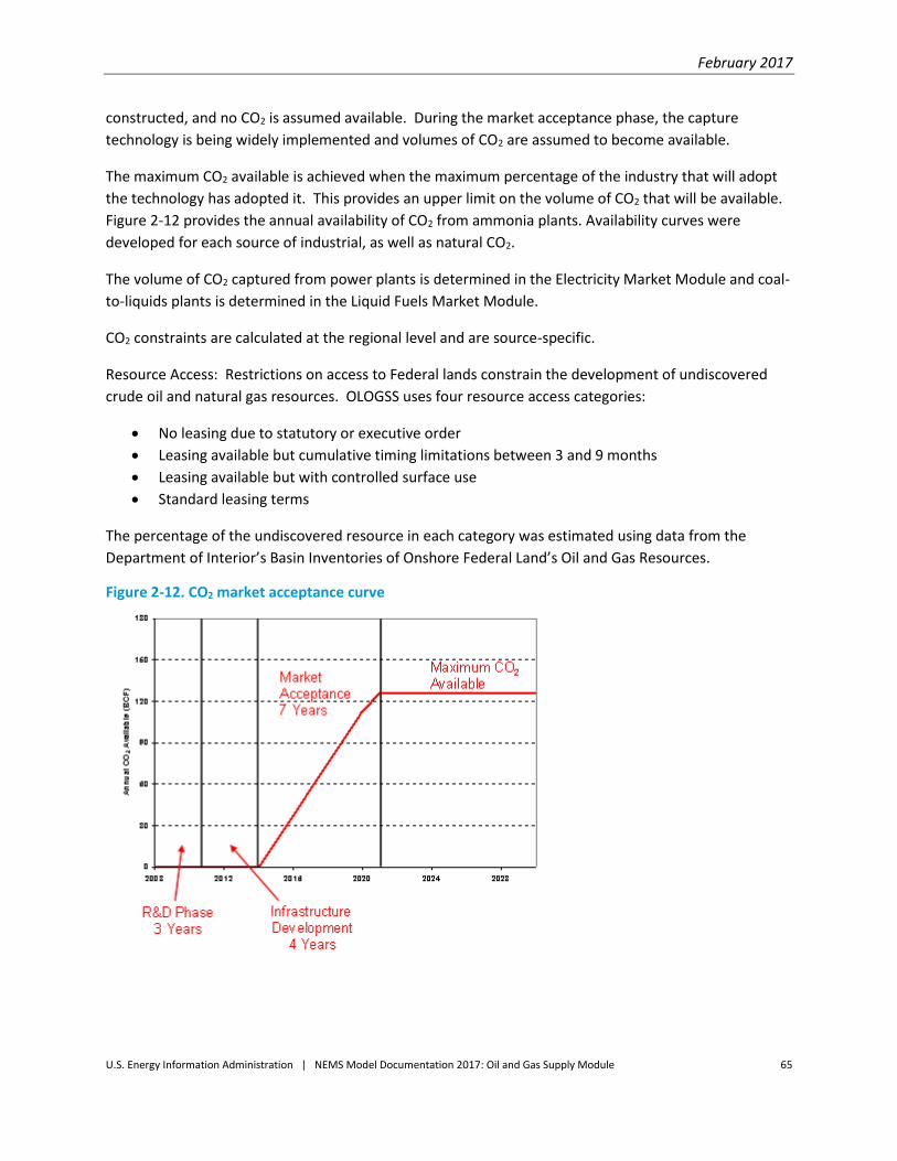
February 2017


constructed, and no CO2 is assumed available. During the market acceptance phase, the capture

technology is being widely implemented and volumes of CO2 are assumed to become available.

The maximum CO2 available is achieved when the maximum percentage of the industry that will adopt

the technology has adopted it. This provides an upper limit on the volume of CO2 that will be available.

Figure 2-12 provides the annual availability of CO2 from ammonia plants. Availability curves were

developed for each source of industrial, as well as natural CO2.

The volume of CO2 captured from power plants is determined in the Electricity Market Module and coal-

to-liquids plants is determined in the Liquid Fuels Market Module.

CO2 constraints are calculated at the regional level and are source-specific.

Resource Access: Restrictions on access to Federal lands constrain the development of undiscovered

crude oil and natural gas resources. OLOGSS uses four resource access categories:

No leasing due to statutory or executive order

Leasing available but cumulative timing limitations between 3 and 9 months

Leasing available but with controlled surface use

Standard leasing terms

The percentage of the undiscovered resource in each category was estimated using data from the

Department of Interior’s Basin Inventories of Onshore Federal Land’s Oil and Gas Resources.

Figure 2-12. CO2 market acceptance curve

February 2017


Technology

The OLOGSS uses a simplified approach to modeling the impact of technology advancement on U.S.

crude oil and natural gas costs and productivity to better capture a continually changing technological

landscape. This approach incorporates assumptions regarding ongoing innovation in upstream

technologies and reflects the average annual growth rate in natural gas and crude oil resources plus

cumulative production from 1990 between AEO2000 and AEO2015.

Areas in tight oil, tight gas, and shale gas plays are divided into two productivity tiers with different

assumed rates of technology change. The first tier (“Tier 1”) encompasses actively developing areas and

the second tier (“Tier 2”) encompasses areas not yet developing. Once development begins in a Tier 2

area, this area is converted to Tier 1 so technological improvement for continued drilling will reflect the

rates assumed for Tier 1 areas. This conversion captures the effects of diminishing returns on a per-well

basis from (1) decreasing well spacing as development progresses, (2) the quick market penetration of

technologies, and (3) the ready application of industry practices and technologies at the time of

development. The specific assumptions for the annual average rate of technological improvement are

shown in Table 2.6.

Table 2-6. Onshore lower 48 technology assumptions

Crude Oil and Natural

Gas Resource Type Drilling Cost

Lease Equipment &

Operating Cost EUR-Tier 1 EUR-Tier 2

Tight oil -1.00% -0.50% 1.00% 3.00%

Tight gas -1.00% -0.50% 1.00% 3.00%

Shale gas -1.00% -0.50% 1.00% 3.00%

All other -0.25% -0.25% 0.25% 0.25%

Source: U.S. Energy Information Administration, Office of Energy Analysis.

Appendix 2.A: Onshore Lower 48 Data Inventory

Variable Name Variable Type Description Unit

AAPI Input API gravity

AARP Input CO2 source acceptance rate

ABO Variable Current formation volume factor bbl/stb

ABOI Input Initial formation volume factor bbl/stb

ABTU Variable Btu content Btu/cf

ACER Input ACE rate %

ACHGASPROD Input Cumulative historical natural gas production MMcf

ACHOILPROD Input Cumulative historical crude oil production Mbbl

ACO2CONT Input CO2 impurity content %

ACRDTYPE Variable Crude type category

ADEPTH Input Depth Ft

February 2017



ADGGLA Variable Depletable items in the year (G&G and lease

acquisition cost)

K$

ADJGAS Variable National natural gas drilling adjustment factor Fraction

ADJGROSS Variable Adjusted gross revenue K$

ADJOIL Variable National crude oil drilling adjustment factor Fraction

ADOILPRICE Variable Adjusted crude oil price $/bbl

ADVANCED Variable Patterns to be developed using advanced

technology

Fraction

AECON_LIFE Variable Economic life of the project Years

AFLP Input Portion of reservoir on federal lands Fraction

AGAS_GRAV Input Natural gas gravity

AGOR Input Gas/oil ratio Mcf/bbl

AH2SCONT Input H2S impurity content %

AHCPV Variable Hydro Carbon Pore Volume 0.4 HCPV

AHEATVAL Input Heat content of natural gas Btu/cf

AINJINJ Input Annual injectant injected Mbbl, Mcf, Mlbs

AINJRECY Variable Annual injectant recycled Mbbl, Mcf

AIRSVGAS Variable End of year inferred natural gas reserves MMcf

AIRSVOIL Variable End-of-year inferred crude oil reserves Mbbl

ALATLEN Input Lateral length Ft

ALATNUM Input Number of laterals

ALYRGAS Input Last year of historical natural gas production MMcf

ALYROIL Input Last year of historical crude oil production Mbbl

AMINT Variable Alternative minimum income tax K$

AMOR Variable Intangible investment depreciation amount K$

AMOR_BASE Variable Amortization base K$

AMORSCHL Input Annual fraction amortized Fraction

AMT Input Alternative minimum tax K$

AMTRATE Input Alternative minimum tax rate K$

AN2CONT Input N2 impurity content %

ANGL Input Natural gas plant liquids factor bbl/MMcf

ANGPLBU Input Butane share of NGPL composition Fraction

ANGPLET Input Ethane share of NGPL composition Fraction

ANGPLIS Input Isobutane share of NGPL composition Fraction

ANGPLPP Input Pentane plus share of NGPL composition Fraction

ANGPLPR Input Propane share of NGPL composition Fraction

ANUMACC Input Number of accumulations

ANWELLGAS Input Number of natural gas wells

ANWELLINJ Input Number of injection wells

ANWELLOIL Input Number of crude oil wells

February 2017



AOAM Variable Annual fixed O&M cost K$

AOGIP Variable Original Gas in Place Bcf

AOILVIS Input Crude Oil viscosity CP

AOOIP Variable Original Oil In Place Mbbl

AORGOOIP Input Original OOIP Mbbl

APATSIZ Input Pattern size Acres

APAY Input Net pay Ft

APD Variable Annual percent depletion K$

APERM Input Permeability MD

APHI Input Porosity %

APLAY_CDE Input Play number

APRESIN Variable Initial pressure PSIA

APRODCO2 Input Annual CO2 production MMcf

APRODGAS Input Annual natural gas production MMcf

APRODNGL Input Annual NGL production Mbbl

APRODOIL Input Annual crude oil production Mbbl

APRODWAT Input Annual water production Mbbl

APROV Input Province

AREGION Input Region number

ARESACC Input Resource Access

ARESFLAG Input Resource flag

ARESID Input Reservoir ID number

ARESVGAS Variable End-of-year proved natural gas reserves

ARESVOIL Variable End-of-year proved crude oil reserves Mbbl

ARRC Input Railroad Commission District

ASC Input Reservoir Size Class

ASGI Variable Gas saturation %

ASOC Input Current oil saturation %

ASOI Input Initial oil saturation %

ASOR Input Residual oil saturation %

ASR_ED Input Number of years after economic life of ASR

ASR_ST Input Number of years before economic life of ASR

ASULFOIL Input Sulfur content of crude oil %

ASWI Input Initial water saturation %

ATCF Variable After tax cash flow K$

ATEMP Variable Reservoir temperature °F

ATOTACRES Input Total area Acres

ATOTCONV Input Number of conversions from producing wells to

injecting wells per pattern

ATOTINJ Input Number of new injectors drilled per pattern

February 2017



ATOTPAT Input Total number of patterns

ATOTPROD Input Number of new producers drilled per pattern

ATOTPS Input Number of primary wells converted to

secondary wells per pattern

AVDP Input Dykstra Parsons coefficient

AWATINJ Input Annual water injected Mbbl

AWOR Input Water/oil ratio bbl/bbl

BAS_PLAY Input Basin number

BASEGAS Input Base natural gas price used for normalization of

capital and operating costs

$/Mcf

BASEOIL Input Base crude oil price used for normalization of

capital and operating costs

K$

BSE_AVAILCO2 Variable Base annual volume of CO2 available by region Bcf

CAP_BASE Variable Capital to be depreciated K$

CAPMUL Input Capital constraints multiplier

CATCF Variable Cumulative discounted cash flow K$

CHG_ANNSEC_FAC Input Change in annual secondary operating cost Fraction

CHG_CHMPNT_FAC Input Change in chemical handling plant cost Fraction

CHG_CMP_FAC Input Change in compression cost Fraction

CHG_CO2PNT_FAC Input Change in CO2 injection/recycling plant cost Fraction

CHG_COMP_FAC Input Change in completion cost Fraction

CHG_DRL_FAC Input Change in drilling cost Fraction

CHG_FAC_FAC Input Change in facilities cost Fraction

CHG_FACUPG_FAC Input Change in facilities upgrade cost Fraction

CHG_FOAM_FAC Input Change in fixed annual O&M cost Fraction

CHG_GNA_FAC Input Change in G&A cost Fraction

CHG_INJC_FAC Input Change in injection cost Fraction

CHG_INJCONV_FAC Input Change in injector conversion cost Fraction

CHG_INJT_FAC Input Change in injectant cost Fraction

CHG_LFT_FAC Input Change in lifting cost Fraction

CHG_OGAS_FAC Input Change in natural gas O&M cost K$

CHG_OINJ_FAC Input Change in injection O&M cost K$

CHG_OOIL_FAC Input Change in oil O&M cost K$

CHG_OWAT_FAC Input Change in water O&M cost K$

CHG_PLYPNT_FAC Input Change in polymer handling plant cost Fraction

CHG_PRDWAT_FAC Input Change in produced water handling plant cost Fraction

CHG_SECWRK_FAC Input Change in secondary workover cost Fraction

CHG_SECCONV_FAC Input Change in secondary conversion cost Fraction

CHG_STM_FAC Input Change in stimulation cost Fraction

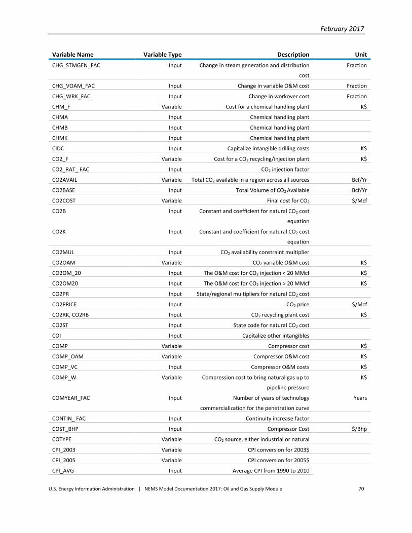
February 2017



CHG_STMGEN_FAC Input Change in steam generation and distribution

cost

Fraction

CHG_VOAM_FAC Input Change in variable O&M cost Fraction

CHG_WRK_FAC Input Change in workover cost Fraction

CHM_F Variable Cost for a chemical handling plant K$

CHMA Input Chemical handling plant

CHMB Input Chemical handling plant

CHMK Input Chemical handling plant

CIDC Input Capitalize intangible drilling costs K$

CO2_F Variable Cost for a CO2 recycling/injection plant K$

CO2_RAT_ FAC Input CO2 injection factor

CO2AVAIL Variable Total CO2 available in a region across all sources Bcf/Yr

CO2BASE Input Total Volume of CO2 Available Bcf/Yr

CO2COST Variable Final cost for CO2 $/Mcf

CO2B Input Constant and coefficient for natural CO2 cost

equation

CO2K Input Constant and coefficient for natural CO2 cost

equation

CO2MUL Input CO2 availability constraint multiplier

CO2OAM Variable CO2 variable O&M cost K$

CO2OM_20 Input The O&M cost for CO2 injection < 20 MMcf K$

CO2OM20 Input The O&M cost for CO2 injection > 20 MMcf K$

CO2PR Input State/regional multipliers for natural CO2 cost

CO2PRICE Input CO2 price $/Mcf

CO2RK, CO2RB Input CO2 recycling plant cost K$

CO2ST Input State code for natural CO2 cost

COI Input Capitalize other intangibles

COMP Variable Compressor cost K$

COMP_OAM Variable Compressor O&M cost K$

COMP_VC Input Compressor O&M costs K$

COMP_W Variable Compression cost to bring natural gas up to

pipeline pressure

K$

COMYEAR_FAC Input Number of years of technology

commercialization for the penetration curve

Years

CONTIN_ FAC Input Continuity increase factor

COST_BHP Input Compressor Cost $/Bhp

COTYPE Variable CO2 source, either industrial or natural

CPI_2003 Variable CPI conversion for 2003$

CPI_2005 Variable CPI conversion for 2005$

CPI_AVG Input Average CPI from 1990 to 2010

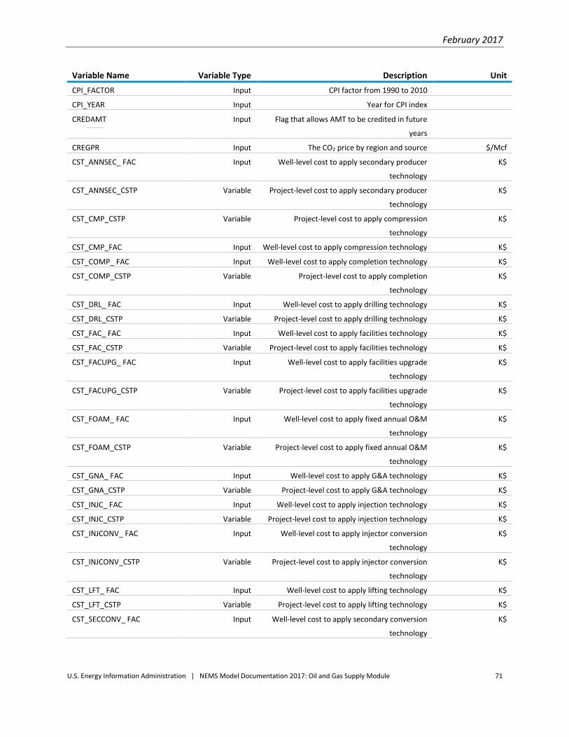
February 2017



CPI_FACTOR Input CPI factor from 1990 to 2010

CPI_YEAR Input Year for CPI index

CREDAMT Input Flag that allows AMT to be credited in future

years

CREGPR Input The CO2 price by region and source $/Mcf

CST_ANNSEC_ FAC Input Well-level cost to apply secondary producer

technology

K$

CST_ANNSEC_CSTP Variable Project-level cost to apply secondary producer

technology

K$

CST_CMP_CSTP Variable Project-level cost to apply compression

technology

K$

CST_CMP_FAC Input Well-level cost to apply compression technology K$

CST_COMP_ FAC Input Well-level cost to apply completion technology K$

CST_COMP_CSTP Variable Project-level cost to apply completion

technology

K$

CST_DRL_ FAC Input Well-level cost to apply drilling technology K$

CST_DRL_CSTP Variable Project-level cost to apply drilling technology K$

CST_FAC_ FAC Input Well-level cost to apply facilities technology K$

CST_FAC_CSTP Variable Project-level cost to apply facilities technology K$

CST_FACUPG_ FAC Input Well-level cost to apply facilities upgrade

technology

K$

CST_FACUPG_CSTP Variable Project-level cost to apply facilities upgrade

technology

K$

CST_FOAM_ FAC Input Well-level cost to apply fixed annual O&M

technology

K$

CST_FOAM_CSTP Variable Project-level cost to apply fixed annual O&M

technology

K$

CST_GNA_ FAC Input Well-level cost to apply G&A technology K$

CST_GNA_CSTP Variable Project-level cost to apply G&A technology K$

CST_INJC_ FAC Input Well-level cost to apply injection technology K$

CST_INJC_CSTP Variable Project-level cost to apply injection technology K$

CST_INJCONV_ FAC Input Well-level cost to apply injector conversion

technology

K$

CST_INJCONV_CSTP Variable Project-level cost to apply injector conversion

technology

K$

CST_LFT_ FAC Input Well-level cost to apply lifting technology K$

CST_LFT_CSTP Variable Project-level cost to apply lifting technology K$

CST_SECCONV_ FAC Input Well-level cost to apply secondary conversion

technology

K$

February 2017



CST_SECCONV_CSTP Variable Project-level cost to apply secondary conversion

technology

K$

CST_SECWRK_ FAC Input Well-level cost to apply secondary workover

technology

K$

CST_SECWRK_CSTP Variable Project-level cost to apply secondary workover

technology

K$

CST_STM_ FAC Input Well-level cost to apply stimulation technology K$

CST_STM_CSTP Variable Project-level cost to apply stimulation

technology

K$

CST_VOAM_ FAC Input Well-level cost to apply variable annual O&M

technology

K$

CST_VOAM_CSTP Variable Project-level cost to apply variable annual O&M

technology

K$

CST_WRK_ FAC Input Well-level cost to apply workover technology K$

CST_WRK_CSTP Variable Project-level cost to apply workover technology K$

CSTP_ANNSEC_ FAC Input Project-level cost to apply secondary producer

technology

K$

CSTP_CMP_ FAC Input Project-level cost to apply compression

technology

K$

CSTP_COMP_ FAC Input Project-level cost to apply completion

technology

K$

CSTP_DRL_ FAC Input Project-level cost to apply drilling technology K$

CSTP_FAC_ FAC Input Project-level cost to apply facilities technology K$

CSTP_FACUPG_ FAC Input Project-level cost to apply facilities upgrade

technology

K$

CSTP_FOAM_ FAC Input Project-level cost to apply fixed annual O&M

technology

K$

CSTP_GNA_ FAC Input Project-level cost to apply G&A technology K$

CSTP_INJC_ FAC Input Project-level cost to apply injection technology K$

CSTP_INJCONV_ FAC Input Project-level cost to apply injector conversion

technology

K$

CSTP_LFT_ FAC Input Project-level cost to apply lifting technology K$

CSTP_SECCONV_ FAC Input Project-level cost to apply secondary conversion

technology

K$

CSTP_SECWRK_ FAC Input Project-level cost to apply secondary workover

technology

K$

CSTP_STM_ FAC Input Project-level cost to apply stimulation

technology

K$

CSTP_VOAM_ FAC Input Project-level cost to apply variable annual O&M

technology

K$

February 2017



CSTP_WRK_ FAC Input Project-level cost to apply workover technology K$

CUTOIL Input Base crude oil price for the adjustment term of

price normalization

$/bbl

DATCF Variable Discounted cash flow after taxes K$

DEP_CRD Variable Depletion credit K$

DEPLET Variable Depletion allowance K$

DEPR Variable Depreciation amount K$

DEPR_OVR Input Annual fraction to depreciate

DEPR_PROC Input Process number for override schedule

DEPR_YR Input Number of years for override schedule

DEPRSCHL Input Annual Fraction Depreciated Fraction

DEPR_SCH Variable Process-specific depreciation schedule Years

DGGLA Variable Depletion base (G&G and lease acquisition cost) K$

DISC_DRL Variable Discounted drilling cost K$

DISC_FED Variable Discounted federal tax payments K$

DISC_GAS Variable Discounted revenue from natural gas sales K$

DISC_INV Variable Discounted investment rate K$

DISC_NDRL Variable Discounted project facilities costs K$

DISC_OAM Variable Discounted O&M cost K$

DISC_OIL Variable Discounted revenue from crude oil sales K$

DISC_ROY Variable Discounted royalty K$

DISC_ST Variable Discounted state tax rate K$

DISCLAG Input Number of years between discovery and first

production

DISCOUNT_RT Input Process discount rates %

DRCAP_D Variable Regional dual-use drilling footage for crude oil

and natural gas development

Ft

DRCAP_G Variable Regional natural gas well drilling footage

constraints

Ft

DRCAP_O Variable Regional crude oil well drilling footage

constraints

Ft

DRILL_FAC Input Drilling rate factor

DRILL_OVER Input Drilling constraints available for footage over

run

%

DRILL_RES Input Development drilling constraints available for

transfer between crude oil and natural gas

%

DRILL_TRANS Input Drilling constraints transfer between regions %

DRILLCST Variable Drill cost by project K$

DRILLL48 Variable Successful well drilling costs 1987$ per well

DRL_CST Variable Drilling cost K$

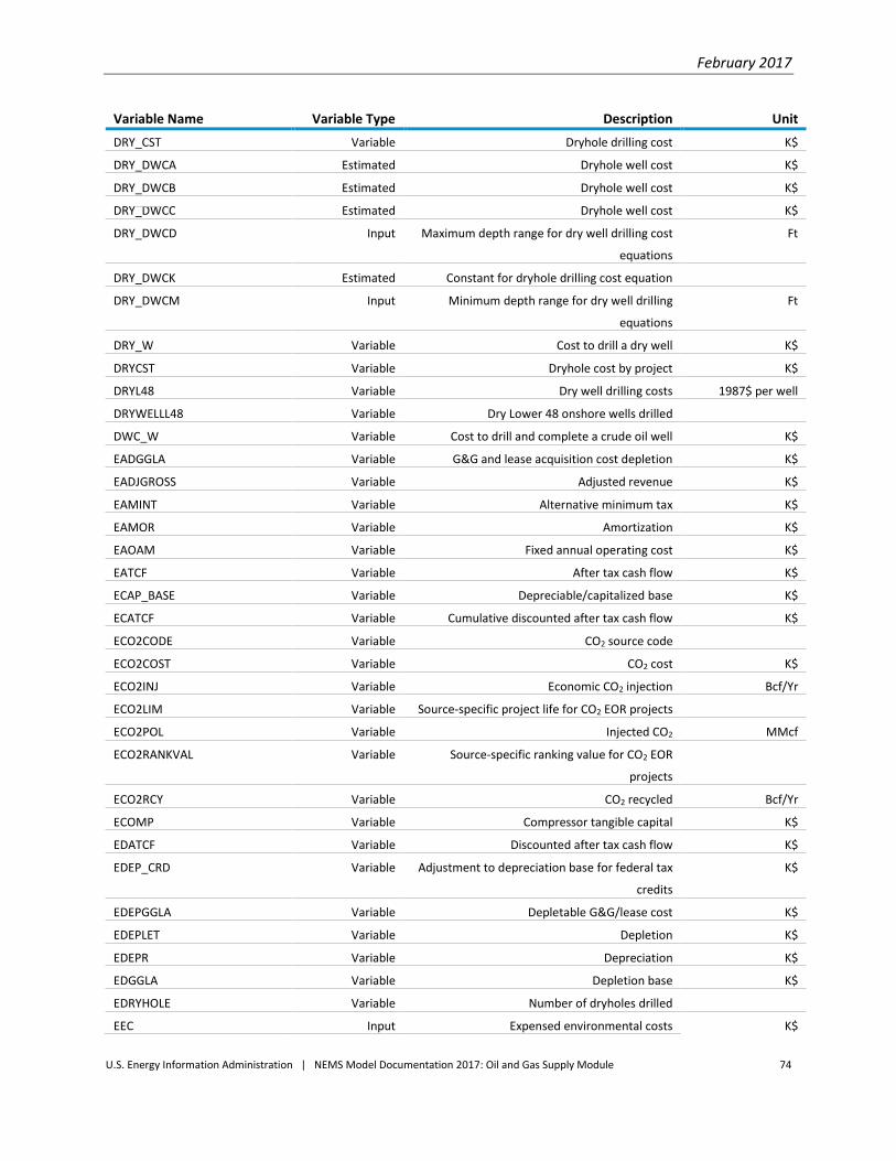
February 2017



DRY_CST Variable Dryhole drilling cost K$

DRY_DWCA Estimated Dryhole well cost K$

DRY_DWCB Estimated Dryhole well cost K$

DRY_DWCC Estimated Dryhole well cost K$

DRY_DWCD Input Maximum depth range for dry well drilling cost

equations

Ft

DRY_DWCK Estimated Constant for dryhole drilling cost equation

DRY_DWCM Input Minimum depth range for dry well drilling

equations

Ft

DRY_W Variable Cost to drill a dry well K$

DRYCST Variable Dryhole cost by project K$

DRYL48 Variable Dry well drilling costs 1987$ per well

DRYWELLL48 Variable Dry Lower 48 onshore wells drilled

DWC_W Variable Cost to drill and complete a crude oil well K$

EADGGLA Variable G&G and lease acquisition cost depletion K$

EADJGROSS Variable Adjusted revenue K$

EAMINT Variable Alternative minimum tax K$

EAMOR Variable Amortization K$

EAOAM Variable Fixed annual operating cost K$

EATCF Variable After tax cash flow K$

ECAP_BASE Variable Depreciable/capitalized base K$

ECATCF Variable Cumulative discounted after tax cash flow K$

ECO2CODE Variable CO2 source code

ECO2COST Variable CO2 cost K$

ECO2INJ Variable Economic CO2 injection Bcf/Yr

ECO2LIM Variable Source-specific project life for CO2 EOR projects

ECO2POL Variable Injected CO2 MMcf

ECO2RANKVAL Variable Source-specific ranking value for CO2 EOR

projects

ECO2RCY Variable CO2 recycled Bcf/Yr

ECOMP Variable Compressor tangible capital K$

EDATCF Variable Discounted after tax cash flow K$

EDEP_CRD Variable Adjustment to depreciation base for federal tax

credits

K$

EDEPGGLA Variable Depletable G&G/lease cost K$

EDEPLET Variable Depletion K$

EDEPR Variable Depreciation K$

EDGGLA Variable Depletion base K$

EDRYHOLE Variable Number of dryholes drilled

EEC Input Expensed environmental costs K$

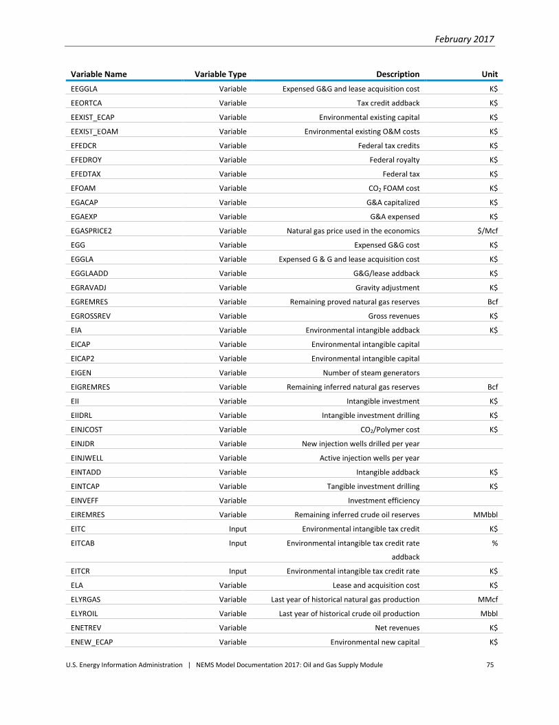
February 2017



EEGGLA Variable Expensed G&G and lease acquisition cost K$

EEORTCA Variable Tax credit addback K$

EEXIST_ECAP Variable Environmental existing capital K$

EEXIST_EOAM Variable Environmental existing O&M costs K$

EFEDCR Variable Federal tax credits K$

EFEDROY Variable Federal royalty K$

EFEDTAX Variable Federal tax K$

EFOAM Variable CO2 FOAM cost K$

EGACAP Variable G&A capitalized K$

EGAEXP Variable G&A expensed K$

EGASPRICE2 Variable Natural gas price used in the economics $/Mcf

EGG Variable Expensed G&G cost K$

EGGLA Variable Expensed G & G and lease acquisition cost K$

EGGLAADD Variable G&G/lease addback K$

EGRAVADJ Variable Gravity adjustment K$

EGREMRES Variable Remaining proved natural gas reserves Bcf

EGROSSREV Variable Gross revenues K$

EIA Variable Environmental intangible addback K$

EICAP Variable Environmental intangible capital

EICAP2 Variable Environmental intangible capital

EIGEN Variable Number of steam generators

EIGREMRES Variable Remaining inferred natural gas reserves Bcf

EII Variable Intangible investment K$

EIIDRL Variable Intangible investment drilling K$

EINJCOST Variable CO2/Polymer cost K$

EINJDR Variable New injection wells drilled per year

EINJWELL Variable Active injection wells per year

EINTADD Variable Intangible addback K$

EINTCAP Variable Tangible investment drilling K$

EINVEFF Variable Investment efficiency

EIREMRES Variable Remaining inferred crude oil reserves MMbbl

EITC Input Environmental intangible tax credit K$

EITCAB Input Environmental intangible tax credit rate

addback

%

EITCR Input Environmental intangible tax credit rate K$

ELA Variable Lease and acquisition cost K$

ELYRGAS Variable Last year of historical natural gas production MMcf

ELYROIL Variable Last year of historical crude oil production Mbbl

ENETREV Variable Net revenues K$

ENEW_ECAP Variable Environmental new capital K$

February 2017



ENEW_EOAM Variable Environmental new O&M costs K$

ENIAT Variable Net income after taxes K$

ENIBT Variable Net income before taxes K$

ENPV Variable Net present value K$

ENV_FAC Input Environmental capital cost multiplier

ENVOP_FAC Input Environmental operating cost multiplier

ENVSCN Input Include environmental costs?

ENYRSI Variable Number of years project is economic

EOAM Variable Variable operating and maintenance K$

EOCA Variable Environmental operating cost addback K$

EOCTC Input Environmental operating cost tax credit K$

EOCTCAB Input Environmental operating cost tax credit rate

addback

%

EOCTCR Input Environmental operating cost tax credit rate K$

EOILPRICE2 Variable Crude oil price used in the economics K$

EORTC Input EOR tax credit K$

EORTCA Variable EOR tax credit addback K$

EORTCAB Input EOR tax credit rate addback %

EORTCP Input EOR tax credit phase out crude oil price K$

EORTCR Input EOR tax credit rate %

EORTCRP Input EOR tax credit applied by year %

EOTC Variable Other tangible capital K$

EPROC_OAM Variable Natural gas processing cost K$

EPRODDR Variable New production wells drilled per year

EPRODGAS Variable Economic natural gas production MMcf

EPRODOIL Variable Economic crude oil production Mbbl

EPRODWAT Variable Economic water production Mbbl

EPRODWELL Variable Active producing wells per year

EREMRES Variable Remaining proved crude oil reserves MMbbl

EROR Variable Rate of return %

EROY Variable Royalty K$

ESEV Variable Severance tax K$

ESHUTIN Variable New shut in wells drilled per year

ESTIM Variable Stimulation cost K$

ESTTAX Variable State tax K$

ESUMP Variable Number of patterns

ESURFVOL Variable Total volume injected MMcf/ Mbbl/ Mlbs

ETAXINC Variable Net income before taxes K$

ETCADD Variable Tax credit addbacks taken from NIAT K$

ETCI Variable Federal tax credit K$

February 2017



ETCIADJ Variable Adjustment for federal tax credit K$

ETI Variable Tangible investments K$

ETOC Variable Total operating cost K$

ETORECY Variable CO2/Surf/Steam recycling volume Bcf/Mbbl/Yr

ETORECY_CST Variable CO2/Surf/Steam recycling cost Bcf/Mbbl/Yr

ETTC Input Environmental tangible tax credit K$

ETTCAB Input Environmental tangible tax credit rate addback %

ETTCR Input Environmental tangible tax credit rate %

EWATINJ Variable Economic water injected Mbbl

EX_CONRES Variable Number of exploration reservoirs

EX_FCRES Variable First exploration reservoir

EXIST_ECAP Variable Existing environmental capital cost K$

EXIST_EOAM Variable Existing environmental O&M cost K$

EXP_ADJ Input Fraction of annual crude oil exploration drilling

which is made available

Fraction

EXP_ADJG Input Fraction of annual natural gas exploration

drilling which is made available

Fraction

EXPA0 Estimated Crude oil exploration well footage A0

EXPA1 Estimated Crude oil exploration well footage A1

EXPAG0 Input Natural gas exploration well footage A0

EXPAG1 Input Natural gas exploration well footage A1

EXPATN Variable Number of active patterns

EXPCDRCAP Variable Regional conventional exploratory drilling

footage constraints

Ft

EXPCDRCAPG Variable Regional conventional natural gas exploration

drilling footage constraint

Ft

EXPGG Variable Expensed G&G cost K$

EXPL_FRAC Input Exploration drilling for conventional crude oil %

EXPL_FRACG Input Exploration drilling for conventional natural gas %

EXPL_MODEL Input Selection of exploration models

EXPLA Variable Expensed lease purchase costs K$

EXPLR_ FAC Input Exploration factor

EXPLR_CHG Variable Change in exploration rate

EXPLSORTIRES Variable Sort pointer for exploration

EXPMUL Input Exploration constraint multiplier

EXPRDL48 Variable Expected Production Oil-MMbbl Gas-Bcf

EXPUDRCAP Variable Regional continuous exploratory drilling footage

constraints

Ft

EXPUDRCAPG Variable Regional continuous natural gas exploratory

drilling footage constraints

Ft

February 2017



FAC_W Variable Facilities upgrade cost K$

FACCOST Variable Facilities cost K$

FACGA Estimated Natural gas facilities costs

FACGB Estimated Natural gas facilities costs

FACGC Estimated Natural gas facilities costs

FACGD Input Maximum depth range for natural gas facilities

costs

Ft

FACGK Estimated Constant for natural gas facilities costs

FACGM Input Minimum depth range for natural gas facilities

costs

Ft

FACUPA Estimated Facilities upgrade cost

FACUPB Estimated Facilities upgrade cost

FACUPC Estimated Facilities upgrade cost

FACUPD Input Maximum depth range for facilities upgrade cost Ft

FACUPK Estimated Constant for facilities upgrade costs

FACUPM Input Minimum depth range for facilities upgrade cost Ft

FCO2 Variable Cost multiplier for natural CO2

FEDRATE Input Federal income tax rate %

FEDTAX Variable Federal tax K$

FEDTAX_CR Variable Federal tax credits K$

FIRST_ASR Variable First year a decline reservoir will be considered

for ASR

FIRST_DEC Variable First year a decline reservoir will be considered

for EOR

FIRSTCOM_FAC Input First year of commercialization for technology

on the penetration curve

FIT Variable Federal income tax K$

FOAM Variable CO2 fixed O&M cost K$

FOAMG_1 Variable Fixed annual operating cost for natural gas 1 K$

FOAMG_2 Variable Fixed annual operating cost for natural gas 2 K$

FOAMG_W Variable Fixed operating cost for natural gas wells K$

FGASPRICE Input Fixed natural gas price $/Mcf

FOILPRICE Input Fixed crude oil price $/bbl

FPLY Variable Cost multiplier for polymer

FPRICE Input Selection to use fixed prices

FR1L48 Variable Finding rates for new field wildcat drilling Oil-MMbbl per well

Gas-Bcf per well

FR2L48 Variable Finding rates for other exploratory drilling Oil-MMbbl per well

Gas-Bcf per well

February 2017



FR3L48 Variable Finding rates for developmental drilling Oil-MMbbl per well

Gas-Bcf per well

FRAC_CO2 Variable Fraction of CO2 Fraction

FRAC_H2S Variable Fraction of hydrogen sulfide Fraction

FRAC_N2 Variable Fraction of nitrogen Fraction

FRAC_NGL Variable NGL yield Fraction

FWC_W Variable Natural gas facilities costs K$

GA_CAP Variable G&A on capital K$

GA_EXP Variable G&A on expenses K$

GAS_ADJ Input Fraction of annual natural gas drilling which is

made available

Fraction

GAS_CASE Input Filter for all natural gas processes

GAS_DWCA Estimated Horizontal natural gas drilling and completion

costs

GAS_DWCB Estimated Horizontal natural gas drilling and completion

costs

GAS_DWCC Estimated Horizontal natural gas drilling and completion

costs

GAS_DWCD Input Maximum depth range for natural gas well

drilling cost equations

Ft

GAS_DWCK Estimated Constant for natural gas well drilling cost

equations

GAS_DWCM Input Minimum depth range for natural gas well

drilling cost equations

Ft

GAS_FILTER Input Filter for all natural gas processes

GAS_OAM Input Process-specific operating cost for natural gas

production

$/Mcf

GAS_SALES Input Will produced natural gas be sold?

GASA0 Estimated Natural gas footage A0

GASA1 Estimated Natural gas footage A1

GASD0 Input Natural gas drywell footage A0

GASD1 Input Natural gas drywell footage A1

GASPRICE2 Variable Natural gas price dummy to shift price track K$

GASPRICEC Variable Annual natural gas prices used by cash flow K$

GASPRICED Variable Annual natural gas prices used in the drilling

constraints

K$

GASPRICEO Variable Annual natural gas prices used by the model K$

GASPROD Variable Annual natural gas production MMcf

GG Variable G&G cost K$

GG_FAC Input G&G factor

February 2017



GGCTC Input G&G tangible depleted tax credit K$

GGCTCAB Input G&G tangible tax credit rate addback %

GGCTCR Input G&G tangible depleted tax credit rate K$

GGETC Input G&G intangible depleted tax credit K$

GGETCAB Input G&G intangible tax credit rate addback %

GGETCR Input G&G intangible depleted tax credit rate K$

GGLA Variable G&G and lease acquisition addback K$

GMULT_INT Input Natural gas price adjustment factor, intangible

costs

K$

GMULT_OAM Input Natural gas price adjustment factor, O&M K$

GMULT_TANG Input Natural gas price adjustment factor, tangible

costs

K$

GNA_CAP2 Input G&A capital multiplier Fraction

GNA_EXP2 Input G&A expense multiplier Fraction

GPROD Variable Well level natural gas production MMcf

GRAVPEN Variable Gravity penalty K$

GREMRES Variable Remaining proved natural gas reserves MMcf

GROSS_REV Variable Gross revenue K$

H_GROWTH Input Horizontal growth rate %

H_PERCENT Input Crude oil constraint available for horizontal

drilling

%

H_SUCCESS Input Horizontal development well success rate by

region

%

H2SPRICE Input H2S price $/metric ton

HOR_ADJ Input Fraction of annual horizontal drilling which is

made available

Fraction

HOR_VERT Input Split between horizontal and vertical drilling

HORMUL Input Horizontal drilling constraint multiplier

IAMORYR Input Number of years in default amortization

schedule

ICAP Variable Other intangible costs K$

ICST Variable Intangible cost K$

IDCA Variable Intangible drilling capital addback K$

IDCTC Input Intangible drilling cost tax credit K$

IDCTCAB Input Intangible drilling cost tax credit rate addback %

IDCTCR Input Intangible drilling cost tax credit rate K$

IDEPRYR Input Number of years in default depreciation

schedule

IGREMRES Variable Remaining inferred natural gas reserves MMcf

II_DRL Variable Intangible drilling cost K$

February 2017



IINFARSV Variable Initial inferred AD gas reserves Bcf

IINFRESV Variable Initial inferred reserves MMbbl

IMP_CAPCR Input Capacity for NGL cryogenic expander plant MMCf/d

IMP_CAPST Input Capacity for NGL straight refrigeration MMcf/d

IMP_CAPSU Input Capacity for Claus Sulfur Recovery Long ton/day

IMP_CAPTE Input Natural gas processing plant capacity MMcf/d

IMP_CO2_LIM Input Limit on CO2 in natural gas Fraction

IMP_DIS_RATE Input Discount rate for natural gas processing plant

IMP_H2O_LIM Input Limit on H2O in natural gas Fraction

IMP_H2S_LIM Input Limit on H2S in natural gas Fraction

IMP_N2_LIM Input Limit on N2 in natural gas Fraction

IMP_NGL_LIM Input Limit on NGL in natural gas Fraction

IMP_OP_FAC Input Natural gas processing operating factor

IMP_PLT_LFE Input Natural gas processing plant life Years

IMP_THRU Input Throughput

IND_SRCCO2 Input Use industrial source of CO2?

INDUSTRIAL Variable Natural or industrial CO2 source

INFLFAC Input Annual Inflation Factor

INFR_ADG Input Adjustment factor for inferred AD gas reserves Tcf

INFR_CBM Input Adjustment factor for inferred coalbed methane

reserves

Tcf

INFR_DNAG Input Adjustment factor for inferred deep non-

associated gas reserves

Tcf

INFR_OIL Input Adjustment factor for inferred crude oil reserves bbl

INFR_SHL Input Adjustment factor for inferred shale gas

reserves

Tcf

INFR_SNAG Input Adjustment factor for inferred shallow non-

associated gas reserves

Tcf

INFR_THT Input Adjustment factor for inferred tight gas reserves Tcf

INFARSV Variable Inferred AD gas reserves Bcf

INFRESV Variable Inferred reserves, crude oil or natural gas MMbbl, Bcf

INJ Variable Injectant cost K$

INJ_OAM Input Process-specific operating cost for injection $/bbl

INJ_RATE_FAC Input Injection rate increase fraction

INTADD Variable Total intangible addback K$

INTANG_M Variable Intangible cost multiplier

INTCAP Variable Intangible to be capitalized K$

INVCAP Variable Annual total capital investments constraints,

used for constraining projects

MM$

IPDR Input Independent producer depletion rate

February 2017



IRA Input Max alternate minimum tax reduction for

independents

K$

IREMRES Variable Remaining inferred crude oil reserves Mbbl

IUNDARES Variable Initial undiscovered resource MMbbl/Tcf

IUNDRES Variable Initial undiscovered resource MMbbl/Tcf

L48B4YR Input First year of analysis

LA Variable Lease and acquisition cost K$

LACTC Input Lease acquisition tangible depleted tax credit K$

LACTCAB Input Lease acquisition tangible credit rate addback %

LACTCR Input Lease acquisition tangible depleted tax credit

rate

K$

LAETC Input Lease acquisition intangible expensed tax credit K$

LAETCAB Input Lease acquisition intangible tax credit rate

addback

%

LAETCR Input Lease acquisition intangible expensed tax credit

rate

K$

LAST_ASR Variable Last year a decline reservoir will be considered

for ASR

LAST_DEC Variable Last year a decline reservoir will be considered

for EOR

LBC_FRAC Input Lease bonus fraction Fraction

LEASCST Variable Lease cost by project K$

LEASL48 Variable Lease equipment costs 1987$/well

MARK_PEN_FAC Input Ultimate market penetration

MAXWELL Input Maximum number of dryholes per play per year

MAX_API_CASE Input Maximum API gravity Degrees API

MAX_DEPTH_CASE Input Maximum depth Ft

MAX_PERM_CASE Input Maximum permeability

MAX_RATE_CASE Input Maximum production rate

MIN_API_CASE Input Minimum API gravity Degrees API

MIN_DEPTH_CASE Input Minimum depth Ft

MIN_PERM_CASE Input Minimum permeability

MIN_RATE_CASE Input Minimum production rate

MOB_RAT_ FAC Input Change in mobility ratio

MPRD Input Maximum depth range for new producer

equations

Ft

N_CPI Input Number of years

N2PRICE Input N2 price $/Mcf

NAT_AVAILCO2 Input Annual CO2 availability by region Bcf

NAT_DMDGAS Variable Annual natural gas demand in region Bcf/Yr

February 2017



NAT_DRCAP_D Variable National dual use drilling footage for crude oil


Ft

NAT_DRCAP_G Variable National natural gas well drilling footage

constraints

Ft

NAT_DRCAP_O Variable National crude oil well drilling footage

constraints

Ft

NAT_DUAL Variable National dual-use drilling footage for crude oil


Ft

NAT_EXP Variable National exploratory drilling constraint Bcf/Yr

NAT_EXPC Variable National conventional exploratory drilling crude

oil constraint

Mbbl/Yr

NAT_EXPCDRCAP Variable National conventional exploratory drilling

footage constraints

Ft

NAT_EXPCDRCAPG Variable National high-permeability natural gas

exploratory drilling footage constraints

Ft

NAT_EXPCG Variable National conventional exploratory drilling

natural gas constraint

Bcf/Yr

NAT_EXPG Variable National natural gas exploration drilling

constraint

Bcf/Yr

NAT_EXPU Variable National continuous exploratory drilling crude

oil constraint

Mbbl/Yr

NAT_EXPUDRCAP Variable National continuous exploratory drilling footage

constraints

Ft

NAT_EXPUDRCAPG Variable National continuous natural gas exploratory

drilling footage constraints

Ft

NAT_EXPUG Variable National continuous exploratory drilling natural

gas constraint

Bcf/Yr

NAT_GAS Variable National natural gas drilling constraint Bcf/Yr

NAT_GDR Variable National natural gas dry drilling footage Bcf/Yr

NAT_HGAS Variable Annual dry natural gas MMcf

NAT_HOIL Variable Annual crude oil and lease condensates Mbbl

NAT_HOR Variable Horizontal drilling constraint Mbbl/yr

NAT_INVCAP Input Annual total capital investment constraint MM$

NAT_ODR Variable National crude oil dry drilling footage Mbbl/Yr

NAT_OIL Variable National crude oil drilling constraint Mbbl/Yr

NAT_SRCCO2 Input Use natural source of CO2?

NAT_TOT Variable Total national footage Ft

NET_REV Variable Net revenue K$

NEW_ECAP Variable New environmental capital cost K$

NEW_EOAM Variable New environmental O&M cost K$

February 2017



NEW_NRES Variable New total number of reservoirs

NGLPRICE Input NGL price $/gal

NGPLPRD Variable Annual natural gas plant liquids production Mbbl

NGPLPRDBU Variable Annual butane production Mbbl

NGPLPRDET Variable Annual ethane production Mbbl

NGPLPRDIS Variable Annual isobutane production Mbbl

NGPLPRDPP Variable Annual pentanes plus production Mbbl

NGPLPRDPR Variable Annual propane production Mbbl

NIAT Variable Net income after taxes K$

NIBT Variable Net income before taxes K$

NIBTA Variable Net operating income after adjustments before

addback

K$

NIL Input Net income limitations K$

NILB Variable Net income depletable base K$

NILL Input Net income limitation limit K$

NOI Variable Net operating income K$

NOM_YEAR Input Year for nominal dollars

NPR_W Variable Cost to equip a new producer K$

NPRA Estimated Constant for new producer equipment

NPRB Estimated Constant for new producer equipment

NPRC Estimated Constant for new producer equipment

NPRK Estimated Constant for new producer equipment

NPRM Input Minimum depth range for new producer

equations

Ft

NPROD Variable Well-level NGL production MMcf

NRDL48 Variable Proved reserves added by new field discoveries Oil-MMbbl

Gas-Bcf

NREG Input Number of regions

NSHUT Input Number of years after economics life in which

EOR can be considered

NTECH Input Number of technology impacts

NUMPACK Input Number of packages per play per year

NWELL Input Number of wells in continuous exploration

drilling package

OAM Variable Variable O&M cost K$

OAM_COMP Variable Compression O&M K$

OAM_M Variable O&M cost multiplier

OIA Variable Other intangible capital addback K$

OIL_ADJ Input Fraction of annual crude oil drilling which is

made available

Fraction

February 2017



OIL_CASE Input Filter for all crude oil processes

OIL_DWCA Estimated Constant for crude oil well drilling cost

equations

OIL_DWCB Estimated Constant for crude oil well drilling cost

equations

OIL_DWCC Estimated Constant for crude oil well drilling cost

equations

OIL_DWCD Input Maximum depth range for crude oil well drilling

cost equations

Ft

OIL_DWCK Estimated Constant for crude oil well drilling cost

equations

OIL_DWCM Input Minimum depth range for crude oil well drilling

cost equations

Ft

OIL_FILTER Input Filter for all crude oil processes

OIL_OAM Input Process-specific operating cost for crude oil

production

$/bbl

OIL_RAT_ FAC Input Change in crude oil production rate

OIL_RAT_CHG Variable Change in crude oil production rate

OIL_SALES Input Sell crude oil produced from the reservoir?

OILA0 Estimated Oil footage A0

OILA1 Estimated Oil footage A1

OILCO2 Input Fixed crude oil price used for economic pre-

screening of industrial CO2 projects

K$

OILD0 Input Crude oil drywell footage A0

OILD1 Input Crude oil drywell footage A1

OILPRICEC Variable Annual crude oil prices used by cash flow K$

OILPRICED Variable Annual crude oil prices used in the drilling

constraints

K$

OILPRICEO Variable Annual crude oil prices used by the model K$

OILPROD Variable Annual crude oil production Mbbl

OINJ Variable Welllevel injection MMcf

OITC Input Other intangible tax credit K$

OITCAB Input Other intangible tax credit rate addback %

OITCR Input Other intangible tax credit rate K$

OMGA Estimated Fixed annual cost for natural gas $/Well

OMGB Estimated Fixed annual cost for natural gas $/Well

OMGC Estimated Fixed annual cost for natural gas $/Well

OMGD Input Maximum depth range for fixed annual O&M

natural gas cost

Ft

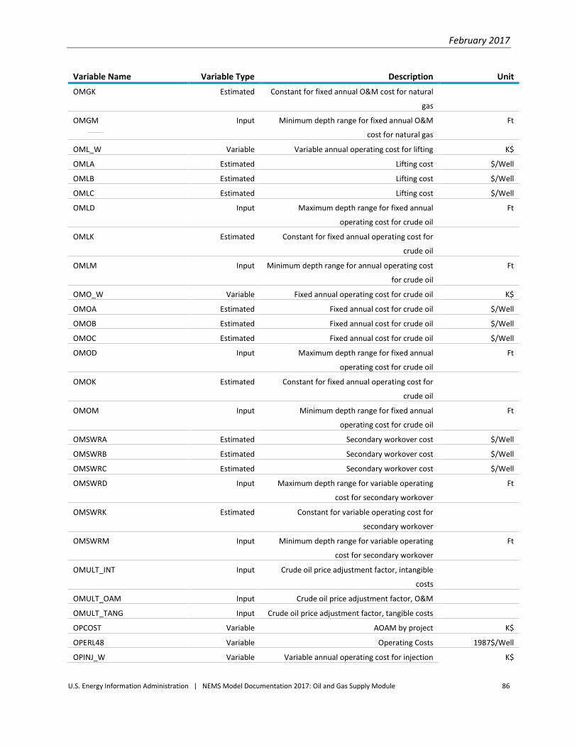
February 2017



OMGK Estimated Constant for fixed annual O&M cost for natural

gas

OMGM Input Minimum depth range for fixed annual O&M

cost for natural gas

Ft

OML_W Variable Variable annual operating cost for lifting K$

OMLA Estimated Lifting cost $/Well

OMLB Estimated Lifting cost $/Well

OMLC Estimated Lifting cost $/Well

OMLD Input Maximum depth range for fixed annual

operating cost for crude oil

Ft

OMLK Estimated Constant for fixed annual operating cost for

crude oil

OMLM Input Minimum depth range for annual operating cost

for crude oil

Ft

OMO_W Variable Fixed annual operating cost for crude oil K$

OMOA Estimated Fixed annual cost for crude oil $/Well

OMOB Estimated Fixed annual cost for crude oil $/Well

OMOC Estimated Fixed annual cost for crude oil $/Well

OMOD Input Maximum depth range for fixed annual


Ft

OMOK Estimated Constant for fixed annual operating cost for

crude oil

OMOM Input Minimum depth range for fixed annual


Ft

OMSWRA Estimated Secondary workover cost $/Well

OMSWRB Estimated Secondary workover cost $/Well

OMSWRC Estimated Secondary workover cost $/Well

OMSWRD Input Maximum depth range for variable operating

cost for secondary workover

Ft

OMSWRK Estimated Constant for variable operating cost for

secondary workover

OMSWRM Input Minimum depth range for variable operating

cost for secondary workover

Ft

OMULT_INT Input Crude oil price adjustment factor, intangible

costs

OMULT_OAM Input Crude oil price adjustment factor, O&M

OMULT_TANG Input Crude oil price adjustment factor, tangible costs

OPCOST Variable AOAM by project K$

OPERL48 Variable Operating Costs 1987$/Well

OPINJ_W Variable Variable annual operating cost for injection K$

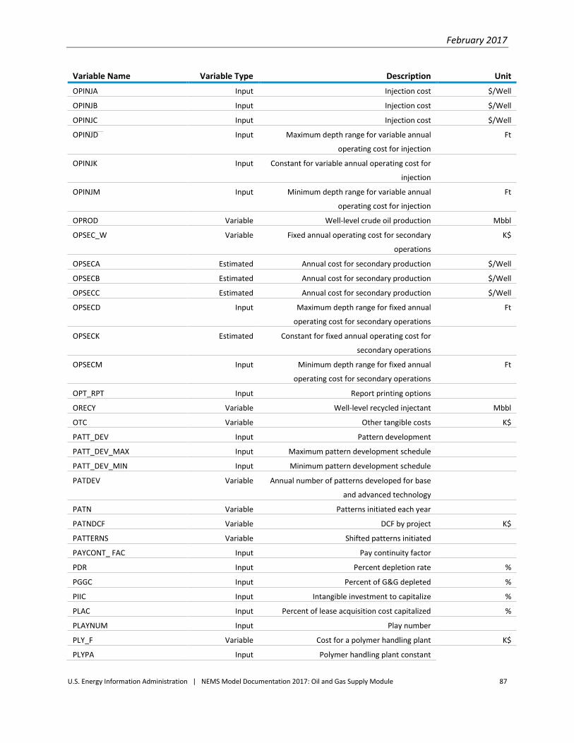
February 2017



OPINJA Input Injection cost $/Well

OPINJB Input Injection cost $/Well

OPINJC Input Injection cost $/Well

OPINJD Input Maximum depth range for variable annual

operating cost for injection

Ft

OPINJK Input Constant for variable annual operating cost for

injection

OPINJM Input Minimum depth range for variable annual

operating cost for injection

Ft

OPROD Variable Well-level crude oil production Mbbl

OPSEC_W Variable Fixed annual operating cost for secondary

operations

K$

OPSECA Estimated Annual cost for secondary production $/Well

OPSECB Estimated Annual cost for secondary production $/Well

OPSECC Estimated Annual cost for secondary production $/Well

OPSECD Input Maximum depth range for fixed annual

operating cost for secondary operations

Ft

OPSECK Estimated Constant for fixed annual operating cost for

secondary operations

OPSECM Input Minimum depth range for fixed annual

operating cost for secondary operations

Ft

OPT_RPT Input Report printing options

ORECY Variable Well-level recycled injectant Mbbl

OTC Variable Other tangible costs K$

PATT_DEV Input Pattern development

PATT_DEV_MAX Input Maximum pattern development schedule

PATT_DEV_MIN Input Minimum pattern development schedule

PATDEV Variable Annual number of patterns developed for base

and advanced technology

PATN Variable Patterns initiated each year

PATNDCF Variable DCF by project K$

PATTERNS Variable Shifted patterns initiated

PAYCONT_ FAC Input Pay continuity factor

PDR Input Percent depletion rate %

PGGC Input Percent of G&G depleted %

PIIC Input Intangible investment to capitalize %

PLAC Input Percent of lease acquisition cost capitalized %

PLAYNUM Input Play number

PLY_F Variable Cost for a polymer handling plant K$

PLYPA Input Polymer handling plant constant

February 2017



PLYPK Input Polymer handling plant constant

POLY Input Polymer cost

POLYCOST Variable Polymer cost $/lb

POTENTIAL Variable The number of reservoirs in the resource file

PRICEYR Input First year of prices in price track K$

PRO_REGEXP Input Regional exploration well drilling footage

constraint

Ft

PRO_REGEXPG Input Regional exploration well drilling footage

constraint

Ft

PRO_REGGAS Input Regional natural gas well drilling footage

constraint

Ft

PRO_REGOIL Input Regional crude oil well drilling footage

constraint

Ft

PROB_IMP_FAC Input Probability of industrial implementation

PROB_RD_FAC Input Probability of successful R & D

PROC_CST Variable Processing cost $/Mcf

PROC_OAM Variable Processing and treating cost K$

PROCESS_CASE Input Filter for crude oil and natural gas processes

PROCESS_FILTER Input Filter for crude oil and natural gas processes

PROD_IND_ FAC Input Production impact

PROVACC Input Year file for resource access

PROVNUM Input Province number

PRRATL48 Variable Production to reserves ratio Fraction

PSHUT Input Number of years prior to economic life in which

EOR can be considered

PSI_W Variable Cost to convert a primary well to an injection

well

K$

PSIA Estimated Cost to convert a producer to an injector

PSIB Estimated Cost to convert a producer to an injector

PSIC Estimated Cost to convert a producer to an injector

PSID Input Maximum depth range for producer to injector Ft

PSIK Estimated Constant for producer to injector

PSIM Input Minimum depth range for producer to injector Ft

PSW_W Variable Cost to convert a primary to secondary well K$

PSWA Estimated Cost to convert a primary to secondary well

PSWB Estimated Cost to convert a primary to secondary well

PSWC Estimated Cost to convert a primary to secondary well

PSWD Input Maximum depth range for producer to injector Ft

PSWK Estimated Constant for primary to secondary

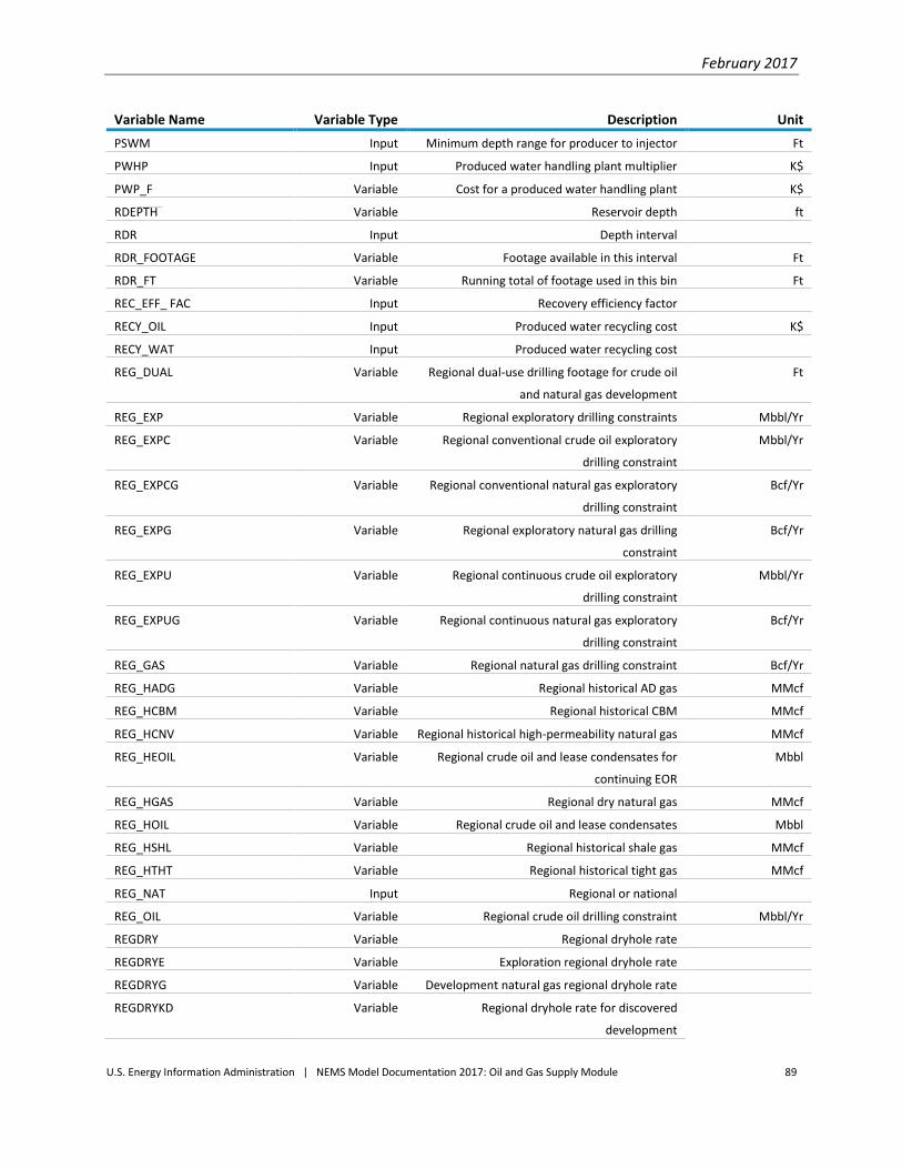
February 2017



PSWM Input Minimum depth range for producer to injector Ft

PWHP Input Produced water handling plant multiplier K$

PWP_F Variable Cost for a produced water handling plant K$

RDEPTH Variable Reservoir depth ft

RDR Input Depth interval

RDR_FOOTAGE Variable Footage available in this interval Ft

RDR_FT Variable Running total of footage used in this bin Ft

REC_EFF_ FAC Input Recovery efficiency factor

RECY_OIL Input Produced water recycling cost K$

RECY_WAT Input Produced water recycling cost

REG_DUAL Variable Regional dual-use drilling footage for crude oil


Ft

REG_EXP Variable Regional exploratory drilling constraints Mbbl/Yr

REG_EXPC Variable Regional conventional crude oil exploratory

drilling constraint

Mbbl/Yr

REG_EXPCG Variable Regional conventional natural gas exploratory

drilling constraint

Bcf/Yr

REG_EXPG Variable Regional exploratory natural gas drilling

constraint

Bcf/Yr

REG_EXPU Variable Regional continuous crude oil exploratory

drilling constraint

Mbbl/Yr

REG_EXPUG Variable Regional continuous natural gas exploratory

drilling constraint

Bcf/Yr

REG_GAS Variable Regional natural gas drilling constraint Bcf/Yr

REG_HADG Variable Regional historical AD gas MMcf

REG_HCBM Variable Regional historical CBM MMcf

REG_HCNV Variable Regional historical high-permeability natural gas MMcf

REG_HEOIL Variable Regional crude oil and lease condensates for

continuing EOR

Mbbl

REG_HGAS Variable Regional dry natural gas MMcf

REG_HOIL Variable Regional crude oil and lease condensates Mbbl

REG_HSHL Variable Regional historical shale gas MMcf

REG_HTHT Variable Regional historical tight gas MMcf

REG_NAT Input Regional or national

REG_OIL Variable Regional crude oil drilling constraint Mbbl/Yr

REGDRY Variable Regional dryhole rate

REGDRYE Variable Exploration regional dryhole rate

REGDRYG Variable Development natural gas regional dryhole rate

REGDRYKD Variable Regional dryhole rate for discovered

development

February 2017



REGDRYUD Variable Regional dryhole rate for undiscovered

development

REGDRYUE Variable Regional dryhole rate for undiscovered

exploration

REGION_CASE Input Filter for OLOGSS region

REGION_FILTER Input Filter for OLOGSS region

REGSCALE_CBM Input Regional historical daily CBM gas production for

the last year of history

Bcf

REGSCALE_CNV Input Regional historical daily high-permeability

natural gas production for the last year of

history

Bcf

REGSCALE_GAS Input Regional historical daily natural gas production

for the last year of history

Bcf

REGSCALE_OIL Input Regional historical daily crude oil production for


Mbbl

REGSCALE_SHL Input Regional historical daily shale gas production for


Bcf

REGSCALE_THT Input Regional historical daily tight gas production for


Bcf

REM_AMOR Variable Remaining amortization base K$

REM_BASE Variable Remaining depreciation base K$

REMRES Variable Remaining proved crude oil reserves Mbbl

RESADL48 Variable Total additions to proved reserves Oil-MMbbl

Gas-Bcf

RESBOYL48 Variable End of year reserves for current year Oil-MMbbl

Gas-Bcf

RES_CHR_ FAC Input Reservoir characterization cost $/Cumulative BOE

RES_CHR_CHG Variable Reservoir characterization cost $/Cumulative BOE

RESV_ADGAS Input Historical AD gas reserves Tcf

RESV_CBM Input Historical coalbed methane reserves Tcf

RESV_CONVGAS Input Historical high-permeability dry natural gas

reserves

Tcf

RESV_OIL Input Historical crude oil and lease condensate

reserves

Bbbl

RESV_SHL Input Historical shale gas reserves Tcf

RESV_THT Input Historical tight gas reserves Tcf

RGR Input Annual drilling growth rate

RIGSL48 Variable Available rigs Rigs

RNKVAL Input Ranking criteria for the projects

ROR Variable Rate of return %

February 2017



ROYALTY Variable Royalty K$

RREG Variable Reservoir region

RRR Input Annual drilling retirement rate

RUNTYPE Input Resources selected to evaluate in the Timing

subroutine

RVALUE Variable Reservoir technical crude oil production Mbbl

SCALE_DAY Input Number of days in the last year of history Days

SCALE_GAS Input Historical daily natural gas production for the

last year of history

Bcf

SCALE_OIL Input Historical daily crude oil production for the last

year of history

Mbbl

SEV_PROC Variable Process code

SEV_TAX Variable Severance tax K$

SFIT Variable Alternative minimum tax K$

SKIN_FAC Input Skin factor

SKIN_CHG Variable Change in skin amount

SMAR Input Six month amortization rate %

SPLIT_ED Input Split exploration and development

SPLIT_OG Input Split crude oil and natural gas constraints

STARTPR Variable First year a pattern is initiated

STATE_TAX Variable State tax K$

STIM Variable Stimulation cost K$

STIM_A, STIM_B Input Coefficients for natural gas/oil stimulation cost K$

STIM_W Variable Natural gas well stimulation cost K$

STIM_YR Input Number of years between stimulations of

natural gas/oil wells

STIMFAC Input Stimulation efficiency factor

STL Variable State identification number

STMGA Input Steam generator cost multiplier

STMM_F Variable Cost for steam manifolds and generators K$

STMMA Input Steam manifold/pipeline multiplier

SUCCHDEV Variable Horizontal development well success rate by

region

Fraction

SUCDEVE Input Developmental well dryhole rate by region %

SUCDEVG Variable Final developmental natural gas well success

rate by region

Fraction

SUCDEVO Variable Final developmental crude oil well success rate

by region

Fraction

SUCEXP Input Undiscovered exploration well dryhole rate by

region

%

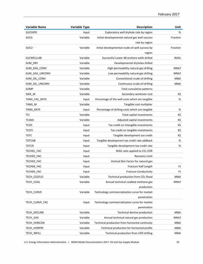
February 2017



SUCEXPD Input Exploratory well dryhole rate by region %

SUCG Variable Initial developmental natural gas well success

rate by region

Fraction

SUCO Variable Initial developmental crude oil well success by

region

Fraction

SUCWELLL48 Variable Successful Lower 48 onshore wells drilled Wells

SUM_DRY Variable Developmental dryholes drilled

SUM_GAS_CONV Variable High-permeability natural gas drilling MMcf

SUM_GAS_UNCONV Variable Low-permeability natural gas drilling MMcf

SUM_OIL_CONV Variable Conventional crude oil drilling Mbbl

SUM_OIL_UNCONV Variable Continuous crude oil drilling Mbbl

SUMP Variable Total cumulative patterns

SWK_W Variable Secondary workover cost K$

TANG_FAC_RATE Input Percentage of the well costs which are tangible %

TANG_M Variable Tangible cost multiplier

TANG_RATE Input Percentage of drilling costs which are tangible %

TCI Variable Total capital investments K$

TCIADJ Variable Adjusted capital investments K$

TCOII Input Tax credit on intangible investments K$

TCOTI Input Tax credit on tangible investments K$

TDTC Input Tangible development tax credit K$

TDTCAB Input Tangible development tax credit rate addback %

TDTCR Input Tangible development tax credit rate %

TECH01_FAC Input WAG ratio applied to CO2 EOR

TECH02_FAC Input Recovery Limit

TECH03_FAC Input Vertical Skin Factor for natural gas

TECH04_FAC Input Fracture Half Length Ft

TECH05_FAC Input Fracture Conductivity Ft

TECH_CO2FLD Variable Technical production from CO2 flood Mbbl

TECH_COAL Variable Annual technical coalbed methane gas

production

MMcf

TECH_CURVE Variable Technology commercialization curve for market

penetration

TECH_CURVE_FAC Input Technology commercialization curve for market

penetration

TECH_DECLINE Variable Technical decline production Mbbl

TECH_GAS Variable Annual technical natural gas production MMcf

TECH_HORCON Variable Technical production from horizontal continuity Mbbl

TECH_HORPRF Variable Technical production for horizontal profile Mbbl

TECH_INFILL Variable Technical production from infill drilling Mbbl

February 2017



TECH_NGL Variable Annual technical NGL production Mbbl

TECH_OIL Variable Annual technical crude oil production Mbbl

TECH_PLYFLD Variable Technical production from polymer injection Mbbl

TECH_PRFMOD Variable Technical production from profile modification Mbbl

TECH_PRIMARY Variable Technical production from primary sources Mbbl

TECH_RADIAL Variable Technical production from conventional radial

flow

MMcf

TECH_SHALE Variable Annual technical shale gas production MMcf

TECH_STMFLD Variable Technical production from steam flood Mbbl

TECH_TIGHT Variable Annual technical tight gas production MMcf

TECH_TIGHTG Variable Technical tight gas production MMcf

TECH_UCOALB Variable Technical undiscovered coalbed methane

production

MMcf

TECH_UCONTO Variable Technical undiscovered continuous crude oil

production

Mbbl

TECH_UCONVG Variable Technical low-permeability natural gas

production

MMcf

TECH_UCONVO Variable Technical undiscovered conventional crude oil

production

Mbbl

TECH_UGCOAL Variable Annual technical developing coalbed methane

gas production

MMcf

TECH_UGSHALE Variable Annual technical developing shale gas

production

MMcf

TECH_UGTIGHT Variable Annual technical developing tight gas

production

MMcf

TECH_USHALE Variable Technical undiscovered shale gas production MMcf

TECH_UTIGHT Variable Technical undiscovered tight gas production MMcf

TECH_WATER Variable Technical production from waterflood Mbbl

TECH_WTRFLD Variable Technical production from waterflood Mbbl

TGGLCD Variable Total G & G cost K$

TI Variable Tangible costs K$

TI_DRL Variable Tangible drilling cost K$

TIMED Variable Timing flag

TIMEDYR Variable Year in which the project is timed

TOC Variable Total operating costs K$

TORECY Variable Annual water injection Mbbl

TORECY_CST Variable Water injection cost K$

TOTHWCAP Variable Total horizontal drilling footage constraint Ft

TOTINJ Variable Annual water injection Mbbl

TOTMUL Input Total drilling constraint multiplier

February 2017



TOTSTATE Variable Total state severance tax K$

UCNT Variable Number of undiscovered reservoirs

UDEPTH Variable Reservoir depth K$

UMPCO2 Input CO2 ultimate market acceptance

UNAME Variable Reservoir identifier

UNDARES Variable Undiscovered resource, AD gas or lease

condensate

Bcf, MMbbl

UNDRES Variable Undiscovered resource MMbbl, cf

UREG Variable Reservoir region

USE_AVAILCO2 Variable Used annual volume of CO2 by region Bcf

USE_RDR Input Use rig depth rating

USEAVAIL Variable Used annual CO2 volume by region across all

sources

Bcf

USECAP Variable Annual total capital investment constraints,

used by projects

MM$

UVALUE Variable Reservoir undiscovered crude oil production Mbbl

UVALUE2 Variable Reservoir undiscovered natural gas production MMcf

VEORCP Input Volumetric EOR cutoff %

VIABLE Variable The number of economically viable reservoirs

VOL_SWP_ FAC Input Sweep volume factor

VOL_SWP_CHG Variable Change in sweep volume

WAT_OAM Input Process-specific operating cost for water

production

$/bbl

WATINJ Variable Annual water injection Mbbl

WATPROD Variable Annual water production Mbbl

WELLSL48 Variable Lower 48 onshore wells drilled Wells

WINJ Variable Well level water injection Mbbl

WPROD Variable Well level water production Mbbl

WRK_W Variable Cost for well workover K$

WRKA Estimated Constant for workover cost equations

WRKB Estimated Constant for workover cost equations

WRKC Estimated Constant for workover cost equations

WRKD Input Maximum depth range for workover cost Ft

WRKK Estimated Constant for workover cost equations

WRKM Input Minimum depth range for workover cost Ft

XCAPBASE Variable Cumulative cap stream

XCUMPROD Variable Cumulative production Mbbl

XPATN Variable Active patterns each year

XPP1 Variable Number of new producers drilled per pattern

XPP2 Variable Number of new injectors drilled per pattern

February 2017



XPP3 Variable Number of producers converted to injectors

XPP4 Variable Number of primary wells converted to

secondary wells

XROY Input Royalty rate %

YEARS_STUDY Input Number of years of analysis

YR1 Input Number of years for tax credit on tangible

investments

YR2 Input Number of years for tax credit on intangible

investments

YRDI Input Years to develop infrastructure

YRDT Input Years to develop technology

YRMA Input Years to reach full capacity

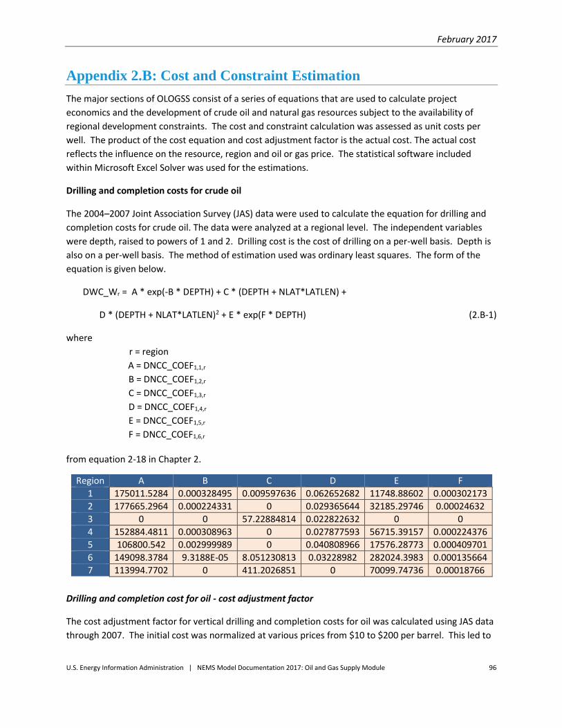
February 2017


Appendix 2.B: Cost and Constraint Estimation

The major sections of OLOGSS consist of a series of equations that are used to calculate project

economics and the development of crude oil and natural gas resources subject to the availability of

regional development constraints. The cost and constraint calculation was assessed as unit costs per

well. The product of the cost equation and cost adjustment factor is the actual cost. The actual cost

reflects the influence on the resource, region and oil or gas price. The statistical software included

within Microsoft Excel Solver was used for the estimations.

Drilling and completion costs for crude oil

The 2004–2007 Joint Association Survey (JAS) data were used to calculate the equation for drilling and

completion costs for crude oil. The data were analyzed at a regional level. The independent variables

were depth, raised to powers of 1 and 2. Drilling cost is the cost of drilling on a per-well basis. Depth is

also on a per-well basis. The method of estimation used was ordinary least squares. The form of the

equation is given below.

DWC_Wr = A * exp(-B * DEPTH) + C * (DEPTH + NLAT*LATLEN) +

D * (DEPTH + NLAT*LATLEN)2 + E * exp(F * DEPTH) (2.B-1)

where

r = region

A = DNCC_COEF1,1,r

B = DNCC_COEF1,2,r

C = DNCC_COEF1,3,r

D = DNCC_COEF1,4,r

E = DNCC_COEF1,5,r

F = DNCC_COEF1,6,r

from equation 2-18 in Chapter 2.

Region A B C D E F

1 175011.5284 0.000328495 0.009597636 0.062652682 11748.88602 0.000302173

2 177665.2964 0.000224331 0 0.029365644 32185.29746 0.00024632

3 0 0 57.22884814 0.022822632 0 0

4 152884.4811 0.000308963 0 0.027877593 56715.39157 0.000224376

5 106800.542 0.002999989 0 0.040808966 17576.28773 0.000409701

6 149098.3784 9.3188E-05 8.051230813 0.03228982 282024.3983 0.000135664

7 113994.7702 0 411.2026851 0 70099.74736 0.00018766

Drilling and completion cost for oil - cost adjustment factor

The cost adjustment factor for vertical drilling and completion costs for oil was calculated using JAS data

through 2007. The initial cost was normalized at various prices from $10 to $200 per barrel. This led to

February 2017


the development of a series of intermediate equations and the calculation of costs at specific prices and

fixed depths. The differentials between estimated costs across the price range and fixed costs at $50

per barrel were then calculated. The cost factor equation was then estimated using the differentials.

The method of estimation used was ordinary least squares. The form of the equation is given below:

Cost = β0 + β1 * Oil Price + β2 * Oil Price2 + β3 * Oil Price3 (2.B-2)

Northeast Region:

Gulf Coast Region:

Regression Statistics

Multiple R 0.993325966

R Square 0.986696475

Adjusted R Square 0.986411399

Standard Error 0.029280014

Observations 144

ANOVA

df SS MS F Significance F

Regression 3 8.901997029 2.967332343 3461.175482 4.4887E-131

Residual 140 0.120024694 0.000857319

Total 143 9.022021723

Coefficients Standard Error t Stat P-value Lower 95% Upper 95% Lower 95.0% Upper 95.0%

β0 0.309616442 0.009839962 31.46520591 2.3349E-65 0.290162308 0.329070576 0.290162308 0.329070576

β1 0.019837121 0.000434252 45.68110123 5.41725E-86 0.018978581 0.020695661 0.018978581 0.020695661

β2 -0.000142411 5.21769E-06 -27.29392193 6.44605E-58 -0.000152727 -0.000132095 -0.000152727 -0.000132095

β3 3.45898E-07 1.69994E-08 20.34770764 1.18032E-43 3.1229E-07 3.79507E-07 3.1229E-07 3.79507E-07



R Square 0.951054265



Observations 144

ANOVA


Regression 3 7.998414341 2.666138114 906.7701736 1.76449E-91

Residual 140 0.411636098 0.002940258

Total 143 8.410050438


β0 0.404677859 0.01822279 22.2072399 1.01029E-47 0.368650426 0.440705292 0.368650426 0.440705292

β1 0.016335847 0.000804199 20.31319148 1.41023E-43 0.014745903 0.017925792 0.014745903 0.017925792

β2 -0.00010587 9.66272E-06 -10.95654411 1.47204E-20 -0.000124974 -8.67663E-05 -0.000124974 -8.67663E-05

β3 2.40517E-07 3.14814E-08 7.639970947 3.10789E-12 1.78277E-07 3.02758E-07 1.78277E-07 3.02758E-07

February 2017


Mid-Continent Region:

Southwest Region:

Rocky Mountain Region:



R Square 0.947852212



Observations 144

ANOVA


Regression 3 8.822668656 2.940889552 848.2258794 1.4872E-89

Residual 140 0.485394925 0.003467107

Total 143 9.308063582


β0 0.309185338 0.019788175 15.62475232 1.738E-32 0.270063053 0.348307623 0.270063053 0.348307623

β1 0.019036286 0.000873282 21.79856116 7.62464E-47 0.017309761 0.020762811 0.017309761 0.020762811

β2 -0.000123667 1.04928E-05 -11.78593913 1.05461E-22 -0.000144412 -0.000102922 -0.000144412 -0.000102922

β3 2.60516E-07 3.41858E-08 7.620611936 3.45556E-12 1.92929E-07 3.28104E-07 1.92929E-07 3.28104E-07



R Square 0.986948023



Observations 144

ANOVA


Regression 3 9.66004438 3.220014793 3528.781511 1.1799E-131

Residual 140 0.127750066 0.0009125

Total 143 9.787794446


β0 0.293837119 0.010151698 28.944627 5.92751E-61 0.273766667 0.313907571 0.273766667 0.313907571

β1 0.020183122 0.00044801 45.05064425 3.35207E-85 0.019297383 0.021068861 0.019297383 0.021068861

β2 -0.000142936 5.38299E-06 -26.55334755 1.63279E-56 -0.000153579 -0.000132294 -0.000153579 -0.000132294

β3 3.44926E-07 1.75379E-08 19.66744699 4.04901E-42 3.10253E-07 3.796E-07 3.10253E-07 3.796E-07



R Square 0.987285538



Observations 144

ANOVA


Regression 3 9.446702681 3.148900894 3623.69457 1.8856E-132

Residual 140 0.121656535 0.000868975

Total 143 9.568359216


β0 0.297270516 0.009906628 30.00723517 7.63744E-63 0.27768458 0.316856451 0.27768458 0.316856451

β1 0.020126228 0.000437194 46.03497443 1.9664E-86 0.019261872 0.020990585 0.019261872 0.020990585

β2 -0.000143079 5.25304E-06 -27.23739215 8.23219E-58 -0.000153465 -0.000132693 -0.000153465 -0.000132693

β3 3.45557E-07 1.71145E-08 20.19080817 2.6538E-43 3.1172E-07 3.79393E-07 3.1172E-07 3.79393E-07

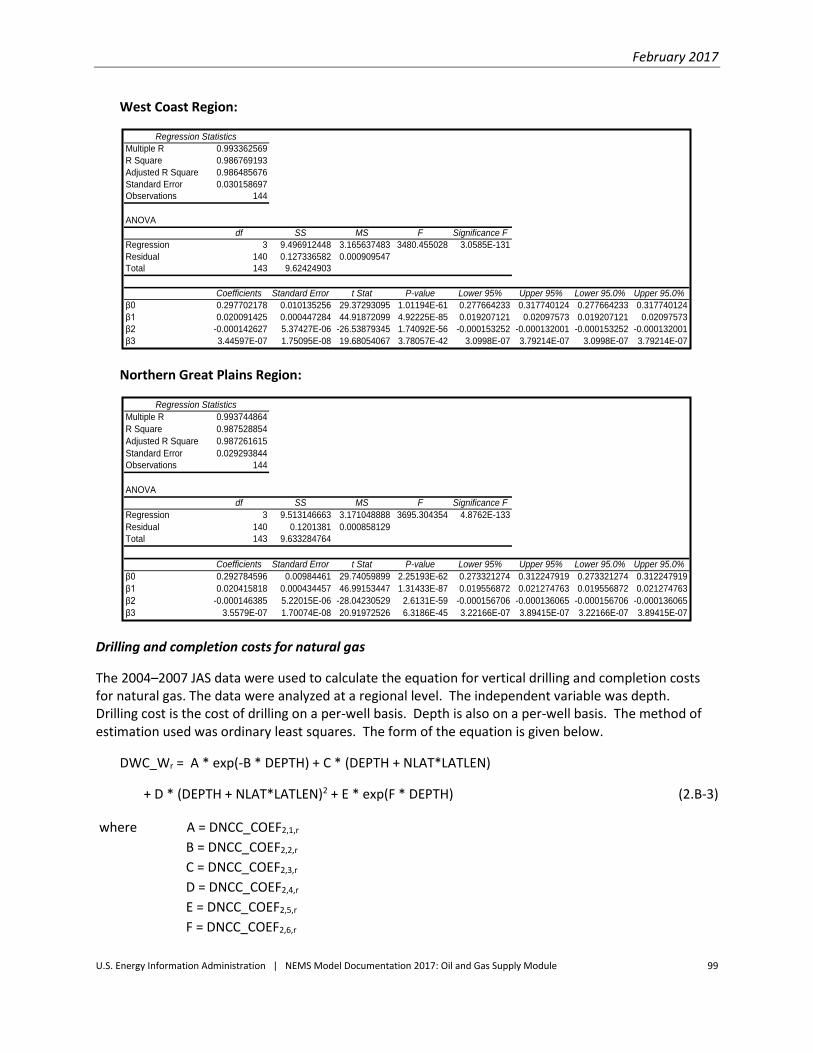
February 2017


West Coast Region:

Northern Great Plains Region:

Drilling and completion costs for natural gas

The 2004–2007 JAS data were used to calculate the equation for vertical drilling and completion costs for natural gas. The data were analyzed at a regional level. The independent variable was depth. Drilling cost is the cost of drilling on a per-well basis. Depth is also on a per-well basis. The method of estimation used was ordinary least squares. The form of the equation is given below.

DWC_Wr = A * exp(-B * DEPTH) + C * (DEPTH + NLAT*LATLEN)

+ D * (DEPTH + NLAT*LATLEN)2 + E * exp(F * DEPTH) (2.B-3)

where A = DNCC_COEF2,1,r

B = DNCC_COEF2,2,r

C = DNCC_COEF2,3,r

D = DNCC_COEF2,4,r

E = DNCC_COEF2,5,r

F = DNCC_COEF2,6,r



R Square 0.986769193



Observations 144

ANOVA


Regression 3 9.496912448 3.165637483 3480.455028 3.0585E-131

Residual 140 0.127336582 0.000909547

Total 143 9.62424903


β0 0.297702178 0.010135256 29.37293095 1.01194E-61 0.277664233 0.317740124 0.277664233 0.317740124

β1 0.020091425 0.000447284 44.91872099 4.92225E-85 0.019207121 0.02097573 0.019207121 0.02097573

β2 -0.000142627 5.37427E-06 -26.53879345 1.74092E-56 -0.000153252 -0.000132001 -0.000153252 -0.000132001

β3 3.44597E-07 1.75095E-08 19.68054067 3.78057E-42 3.0998E-07 3.79214E-07 3.0998E-07 3.79214E-07



R Square 0.987528854



Observations 144

ANOVA


Regression 3 9.513146663 3.171048888 3695.304354 4.8762E-133

Residual 140 0.1201381 0.000858129

Total 143 9.633284764


β0 0.292784596 0.00984461 29.74059899 2.25193E-62 0.273321274 0.312247919 0.273321274 0.312247919

β1 0.020415818 0.000434457 46.99153447 1.31433E-87 0.019556872 0.021274763 0.019556872 0.021274763

β2 -0.000146385 5.22015E-06 -28.04230529 2.6131E-59 -0.000156706 -0.000136065 -0.000156706 -0.000136065

β3 3.5579E-07 1.70074E-08 20.91972526 6.3186E-45 3.22166E-07 3.89415E-07 3.22166E-07 3.89415E-07

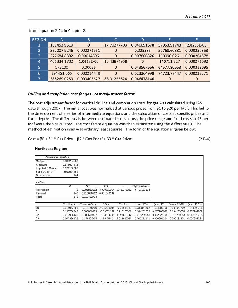
February 2017



REGION A B C D E F

1 139453.9519 0 17.70277703 0.040091678 57953.91743 2.8256E-05

2 362007.9246 0.000271951 0 0.025535 57768.60381 0.000257353

3 277684.8382 0.00014696 0 0.007866326 160096.0261 0.000204878

4 401334.1702 1.0418E-06 15.43874958 0 140711.327 0.000271092

5 175100 0.00056 0 0.043567666 64577.80553 0.000313095

6 394451.065 0.000214449 0 0.023364998 74723.77447 0.000237271

7 388269.0259 0.000405627 88.01255624 0.046478146 0 0

Drilling and completion cost for gas - cost adjustment factor

The cost adjustment factor for vertical drilling and completion costs for gas was calculated using JAS data through 2007. The initial cost was normalized at various prices from $1 to $20 per Mcf. This led to the development of a series of intermediate equations and the calculation of costs at specific prices and fixed depths. The differentials between estimated costs across the price range and fixed costs at $5 per Mcf were then calculated. The cost factor equation was then estimated using the differentials. The method of estimation used was ordinary least squares. The form of the equation is given below:

Cost = β0 + β1 * Gas Price + β2 * Gas Price2 + β3 * Gas Price3 (2.B-4)

Northeast Region:



R Square 0.976607472



Observations 144

ANOVA


Regression 3 9.001833192 3.000611064 1948.272332 6.4218E-114

Residual 140 0.215619522 0.001540139

Total 143 9.217452714


β0 0.315932281 0.013188706 23.95476038 2.2494E-51 0.289857502 0.34200706 0.289857502 0.34200706

β1 0.195760743 0.005820373 33.63371152 6.11526E-69 0.184253553 0.207267932 0.184253553 0.207267932

β2 -0.013906425 0.000699337 -19.88514708 1.29788E-42 -0.015289053 -0.012523798 -0.015289053 -0.012523798

β3 0.000336178 2.27846E-05 14.75458424 2.61104E-30 0.000291131 0.000381224 0.000291131 0.000381224

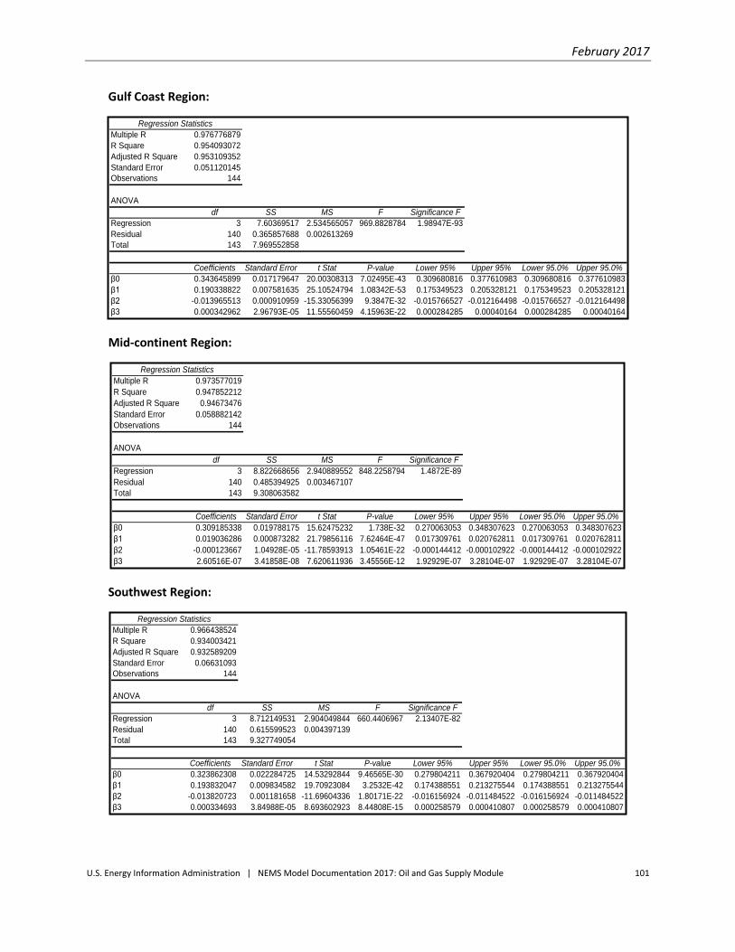
February 2017


Gulf Coast Region:

Mid-continent Region:

Southwest Region:



R Square 0.954093072



Observations 144

ANOVA


Regression 3 7.60369517 2.534565057 969.8828784 1.98947E-93

Residual 140 0.365857688 0.002613269

Total 143 7.969552858


β0 0.343645899 0.017179647 20.00308313 7.02495E-43 0.309680816 0.377610983 0.309680816 0.377610983

β1 0.190338822 0.007581635 25.10524794 1.08342E-53 0.175349523 0.205328121 0.175349523 0.205328121

β2 -0.013965513 0.000910959 -15.33056399 9.3847E-32 -0.015766527 -0.012164498 -0.015766527 -0.012164498

β3 0.000342962 2.96793E-05 11.55560459 4.15963E-22 0.000284285 0.00040164 0.000284285 0.00040164



R Square 0.947852212



Observations 144

ANOVA


Regression 3 8.822668656 2.940889552 848.2258794 1.4872E-89

Residual 140 0.485394925 0.003467107

Total 143 9.308063582


β0 0.309185338 0.019788175 15.62475232 1.738E-32 0.270063053 0.348307623 0.270063053 0.348307623

β1 0.019036286 0.000873282 21.79856116 7.62464E-47 0.017309761 0.020762811 0.017309761 0.020762811

β2 -0.000123667 1.04928E-05 -11.78593913 1.05461E-22 -0.000144412 -0.000102922 -0.000144412 -0.000102922

β3 2.60516E-07 3.41858E-08 7.620611936 3.45556E-12 1.92929E-07 3.28104E-07 1.92929E-07 3.28104E-07



R Square 0.934003421



Observations 144

ANOVA


Regression 3 8.712149531 2.904049844 660.4406967 2.13407E-82

Residual 140 0.615599523 0.004397139

Total 143 9.327749054


β0 0.323862308 0.022284725 14.53292844 9.46565E-30 0.279804211 0.367920404 0.279804211 0.367920404

β1 0.193832047 0.009834582 19.70923084 3.2532E-42 0.174388551 0.213275544 0.174388551 0.213275544

β2 -0.013820723 0.001181658 -11.69604336 1.80171E-22 -0.016156924 -0.011484522 -0.016156924 -0.011484522

β3 0.000334693 3.84988E-05 8.693602923 8.44808E-15 0.000258579 0.000410807 0.000258579 0.000410807

February 2017


Rocky Mountains Region:

West Coast Region:




R Square 0.971394777



Observations 144

ANOVA


Regression 3 8.444274294 2.814758098 1584.737059 8.3614E-108

Residual 140 0.248663418 0.001776167

Total 143 8.692937712


β0 0.32536782 0.014163288 22.97261928 2.42535E-49 0.29736624 0.353369401 0.29736624 0.353369401

β1 0.194045615 0.006250471 31.04496067 1.21348E-64 0.181688099 0.206403131 0.181688099 0.206403131

β2 -0.01396687 0.000751015 -18.59732564 1.18529E-39 -0.015451667 -0.012482073 -0.015451667 -0.012482073

β3 0.000339698 2.44683E-05 13.88318297 4.22503E-28 0.000291323 0.000388073 0.000291323 0.000388073



R Square 0.988321112



Observations 144

ANOVA


Regression 3 8.510960152 2.836986717 3949.147599 4.9307E-135

Residual 140 0.100573131 0.00071838

Total 143 8.611533284


β0 0.325917293 0.009007393 36.18330938 6.29717E-73 0.308109194 0.343725393 0.308109194 0.343725393

β1 0.193657091 0.003975097 48.71757347 1.12458E-89 0.185798111 0.201516072 0.185798111 0.201516072

β2 -0.013893214 0.000477621 -29.08835053 3.2685E-61 -0.014837497 -0.012948932 -0.014837497 -0.012948932

β3 0.000337413 1.5561E-05 21.68318808 1.35414E-46 0.000306648 0.000368178 0.000306648 0.000368178



R Square 0.940968103



Observations 144

ANOVA


Regression 3 7.259587116 2.419862372 743.8663996 8.71707E-86

Residual 140 0.455432229 0.003253087

Total 143 7.715019345


β0 0.352772153 0.0191677 18.40451098 3.34838E-39 0.31487658 0.390667726 0.31487658 0.390667726

β1 0.189510541 0.008458993 22.40344064 3.85701E-48 0.172786658 0.206234423 0.172786658 0.206234423

β2 -0.014060192 0.001016376 -13.83364754 5.65155E-28 -0.016069622 -0.012050761 -0.016069622 -0.012050761

β3 0.000347364 3.31138E-05 10.49000322 2.34854E-19 0.000281896 0.000412832 0.000281896 0.000412832

February 2017


Drilling and completion costs for dry holes

The 2004–2007 JAS data was used to calculate the equation for vertical drilling and completion costs for

dry holes. The data were analyzed at a regional level. The independent variable was depth. Drilling cost

is the cost of drilling on a per-well basis. Depth is also on a per-well basis. The method of estimation

used was ordinary least squares. The form of the equation is given bellow.

DWC_Wr = A * exp(-B * DEPTH) + C * (DEPTH + NLAT*LATLEN)

+ D * (DEPTH + NLAT*LATLEN)2 + E * exp(F * DEPTH) (2.B-5)

where A = DNCC_COEF3,1,r

B = DNCC_COEF3,2,r

C = DNCC_COEF3,3,r

D = DNCC_COEF3,4,r

E = DNCC_COEF3,5,r

F = DNCC_COEF3,6,r

from equations 2-20 and 2-26 in Chapter 2.

REGION A B C D E F

1 373565.4949 0.000335422 0 0.010812916 198571.346 0.000274926

2 145975.4369 0.000298125 5.732481719 0.019485239 139514.304 0.00024177

3 295750.3696 0.000788459 86.14054863 0.013865231 0 0

4 389495.9332 0.000416281 0 0 101481.6339 0.000320498

5 300000 0.000905 0 0.033907497 94160.22038 0.000316633

6 1371262.505 0.000167253 0 0 55899.52234 0.000369903

7 130200 0.003 409.5898966 0.014126494 340333.6789 0.000211981

Drilling and completion cost for dry holes - cost adjustment factor

The cost adjustment factor for vertical drilling and completion costs for dry holes was calculated using JAS data through 2007. The initial cost was normalized at various prices from $10 to $200 per barrel. This led to the development of a series of intermediate equations and the calculation of costs at specific prices and fixed depths. The differentials between estimated costs across the price range and fixed costs at $50 per barrel were then calculated. The cost factor equation was then estimated using the differentials. The method of estimation used was ordinary least squares. The form of the equation is given below:


February 2017


Northeast Region:

Gulf Coast Region:

Mid-Continent Region:



R Square 0.989719089



Observations 144

ANOVA


Regression 3 9.774469405 3.258156468 4492.489925 6.5663E-139

Residual 140 0.101534319 0.000725245

Total 143 9.876003725


β0 0.290689859 0.009050333 32.11924425 1.85582E-66 0.272796865 0.308582854 0.272796865 0.308582854

β1 0.020261651 0.000399405 50.72962235 5.26469E-92 0.019472006 0.021051296 0.019472006 0.021051296

β2 -0.000143294 4.79898E-06 -29.85918012 1.391E-62 -0.000152782 -0.000133806 -0.000152782 -0.000133806

β3 3.45487E-07 1.56352E-08 22.09672004 1.74153E-47 3.14575E-07 3.76399E-07 3.14575E-07 3.76399E-07



R Square 0.986738516



Observations 144

ANOVA


Regression 3 10.44539464 3.481798214 3472.296057 3.5967E-131

Residual 140 0.140383119 0.001002737

Total 143 10.58577776


β0 0.277940175 0.010641812 26.11774938 1.12431E-55 0.256900742 0.298979608 0.256900742 0.298979608

β1 0.020529977 0.000469639 43.71437232 1.71946E-83 0.019601475 0.021458479 0.019601475 0.021458479

β2 -0.000143466 5.64287E-06 -25.42421447 2.53682E-54 -0.000154622 -0.000132309 -0.000154622 -0.000132309

β3 3.43878E-07 1.83846E-08 18.70465533 6.66256E-40 3.07531E-07 3.80226E-07 3.07531E-07 3.80226E-07



R Square 0.968268874



Observations 144

ANOVA


Regression 3 9.856909541 3.285636514 1424.023848 1.1869E-104

Residual 140 0.323020652 0.00230729

Total 143 10.17993019


β0 0.289971748 0.016142592 17.96314638 3.67032E-38 0.258056977 0.32188652 0.258056977 0.32188652

β1 0.020266191 0.000712397 28.44789972 4.71502E-60 0.018857744 0.021674637 0.018857744 0.021674637

β2 -0.000143007 8.55969E-06 -16.70702184 3.8001E-35 -0.00015993 -0.000126084 -0.00015993 -0.000126084

β3 3.44462E-07 2.78877E-08 12.35174476 3.63124E-24 2.89326E-07 3.99597E-07 2.89326E-07 3.99597E-07

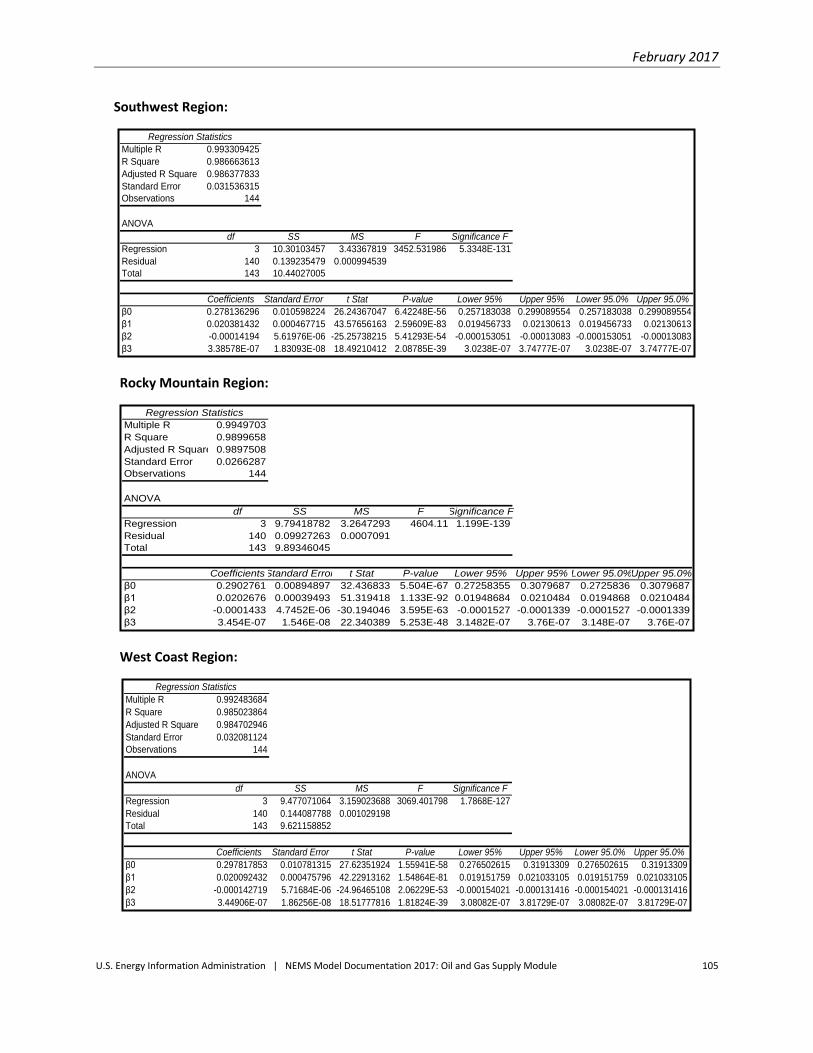
February 2017


Southwest Region:

Rocky Mountain Region:

West Coast Region:



R Square 0.986663613



Observations 144

ANOVA


Regression 3 10.30103457 3.43367819 3452.531986 5.3348E-131

Residual 140 0.139235479 0.000994539

Total 143 10.44027005


β0 0.278136296 0.010598224 26.24367047 6.42248E-56 0.257183038 0.299089554 0.257183038 0.299089554

β1 0.020381432 0.000467715 43.57656163 2.59609E-83 0.019456733 0.02130613 0.019456733 0.02130613

β2 -0.00014194 5.61976E-06 -25.25738215 5.41293E-54 -0.000153051 -0.00013083 -0.000153051 -0.00013083

β3 3.38578E-07 1.83093E-08 18.49210412 2.08785E-39 3.0238E-07 3.74777E-07 3.0238E-07 3.74777E-07



R Square 0.9899658



Observations 144

ANOVA


Regression 3 9.79418782 3.2647293 4604.11 1.199E-139

Residual 140 0.09927263 0.0007091

Total 143 9.89346045

CoefficientsStandard Error t Stat P-value Lower 95% Upper 95% Lower 95.0%Upper 95.0%

β0 0.2902761 0.00894897 32.436833 5.504E-67 0.27258355 0.3079687 0.2725836 0.3079687

β1 0.0202676 0.00039493 51.319418 1.133E-92 0.01948684 0.0210484 0.0194868 0.0210484

β2 -0.0001433 4.7452E-06 -30.194046 3.595E-63 -0.0001527 -0.0001339 -0.0001527 -0.0001339

β3 3.454E-07 1.546E-08 22.340389 5.253E-48 3.1482E-07 3.76E-07 3.148E-07 3.76E-07



R Square 0.985023864



Observations 144

ANOVA


Regression 3 9.477071064 3.159023688 3069.401798 1.7868E-127

Residual 140 0.144087788 0.001029198

Total 143 9.621158852


β0 0.297817853 0.010781315 27.62351924 1.55941E-58 0.276502615 0.31913309 0.276502615 0.31913309

β1 0.020092432 0.000475796 42.22913162 1.54864E-81 0.019151759 0.021033105 0.019151759 0.021033105

β2 -0.000142719 5.71684E-06 -24.96465108 2.06229E-53 -0.000154021 -0.000131416 -0.000154021 -0.000131416

β3 3.44906E-07 1.86256E-08 18.51777816 1.81824E-39 3.08082E-07 3.81729E-07 3.08082E-07 3.81729E-07

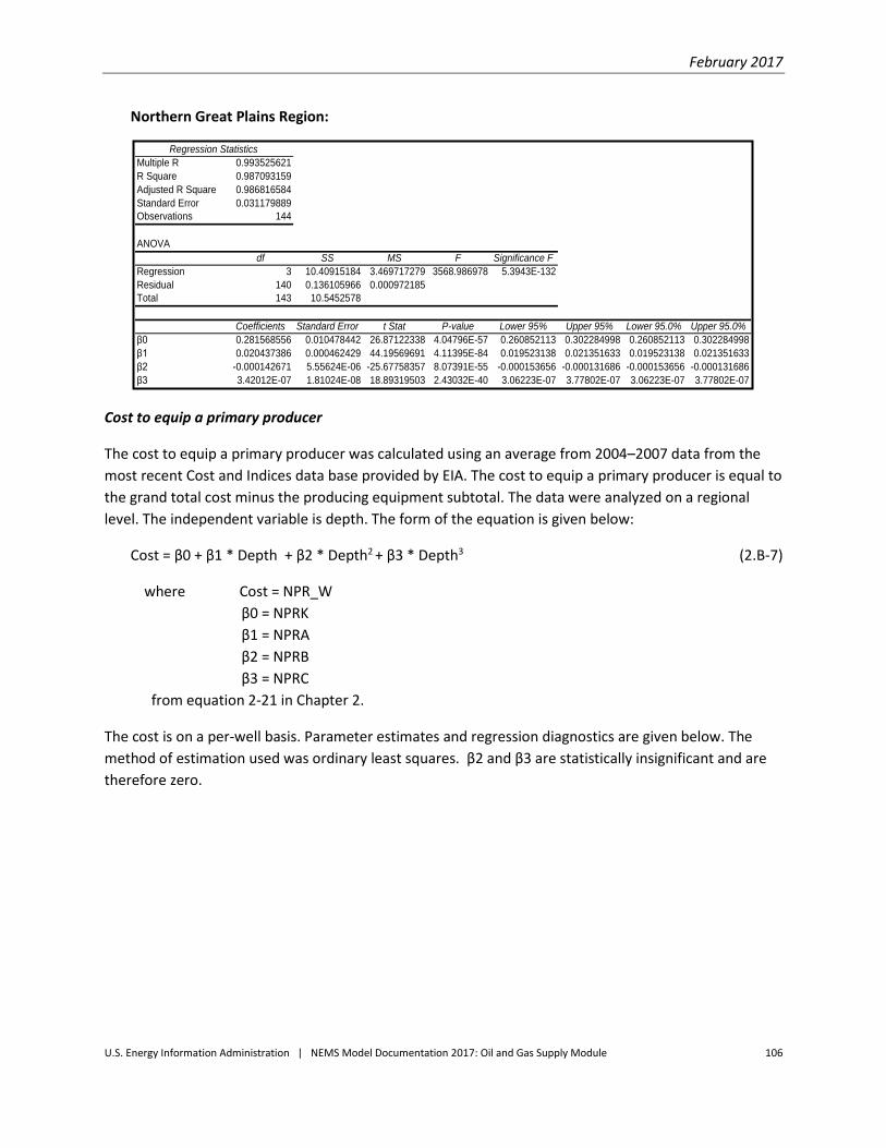
February 2017



Cost to equip a primary producer

The cost to equip a primary producer was calculated using an average from 2004–2007 data from the

most recent Cost and Indices data base provided by EIA. The cost to equip a primary producer is equal to

the grand total cost minus the producing equipment subtotal. The data were analyzed on a regional

level. The independent variable is depth. The form of the equation is given below:

Cost = β0 + β1 * Depth + β2 * Depth2 + β3 * Depth3 (2.B-7)

where Cost = NPR_W

β0 = NPRK

β1 = NPRA

β2 = NPRB

β3 = NPRC


The cost is on a per-well basis. Parameter estimates and regression diagnostics are given below. The

method of estimation used was ordinary least squares. β2 and β3 are statistically insignificant and are

therefore zero.



R Square 0.987093159



Observations 144

ANOVA


Regression 3 10.40915184 3.469717279 3568.986978 5.3943E-132

Residual 140 0.136105966 0.000972185

Total 143 10.5452578


β0 0.281568556 0.010478442 26.87122338 4.04796E-57 0.260852113 0.302284998 0.260852113 0.302284998

β1 0.020437386 0.000462429 44.19569691 4.11395E-84 0.019523138 0.021351633 0.019523138 0.021351633

β2 -0.000142671 5.55624E-06 -25.67758357 8.07391E-55 -0.000153656 -0.000131686 -0.000153656 -0.000131686

β3 3.42012E-07 1.81024E-08 18.89319503 2.43032E-40 3.06223E-07 3.77802E-07 3.06223E-07 3.77802E-07

February 2017


West Texas, applied to OLOGSS regions 2 and 4:


Multiple R 0.921

R Square 0.849



Observations 3

ANOVA


Regression 1 2,163,010.81 2,163,010.81 5.61 0.254415

Residual 1 385,858.01 385,858.01

Total 2 2,548,868.81


β05 1 , 3 1 5 . 4 0 3 4 7 6 0 . 7 8 0 5 6 7 . 4 5 1 0 0 . 0 0 9 4 4 1 , 6 4 8 . 8 1 1 7 6 0 , 9 8 1 . 9 9 5 2 4 1 , 6 4 8 . 8 1 1 7 6 0 , 9 8 1 . 9 9 5 2

β10 . 3 4 0 4 0 . 1 4 3 8 2 . 3 6 7 6 0 . 2 5 4 4 - 1 . 4 8 6 4 2 . 1 6 7 2 - 1 . 4 8 6 4 2 . 1 6 7 2

February 2017


Mid-Continent, applied to OLOGSS region 3:

Rocky Mountains, applied to OLOGSS regions 1, 5, and 7:

West Coast, applied to OLOGSS regions 6:


Multiple R 0.995

R Square 0.990


Standard Error 1,193.14

Observations 3

ANOVA


Regression 1 145,656,740.81 145,656,740.81 102.32 0.06

Residual 1 1,423,576.87 1,423,576.87

Total 2 147,080,317.68


β04 5 , 8 2 1 . 7 1 7 1 , 4 6 1 . 2 8 9 3 1 . 3 5 7 0 . 0 2 0 2 7 , 2 5 4 . 3 6 0 6 4 , 3 8 9 . 0 7 4 2 7 , 2 5 4 . 3 6 0 6 4 , 3 8 9 . 0 7 4

β12 . 7 9 3 0 . 2 7 6 1 0 . 1 1 5 0 . 0 6 3 - 0 . 7 1 6 6 . 3 0 2 - 0 . 7 1 6 6 . 3 0 2


Multiple R 0.9998

R Square 0.9995



Observations 3

ANOVA


Regression 1 105,460,601.42 105,460,601.42 2,093.17 0.01

Residual 1 50,383.23 50,383.23

Total 2 105,510,984.64


β06 2 , 7 0 9 . 3 7 8 2 7 4 . 9 0 9 2 2 8 . 1 1 0 0 . 0 0 3 5 9 , 2 1 6 . 3 4 6 6 6 , 2 0 2 . 4 1 1 5 9 , 2 1 6 . 3 4 6 6 6 , 2 0 2 . 4 1 1

β12 . 3 7 7 0 . 0 5 2 4 5 . 7 5 1 0 . 0 1 4 1 . 7 1 7 3 . 0 3 7 1 . 7 1 7 3 . 0 3 7


Multiple R 0.9095

R Square 0.8272



Observations 4

ANOVA


Regression 1 48,812,671.60 48,812,671.60 9.58 0.09

Residual 2 10,194,785.98 5,097,392.99

Total 3 59,007,457.58


β01 0 6 , 9 5 9 . 7 8 8 2 , 2 1 9 . 1 4 4 4 8 . 1 9 9 0 . 0 0 0 9 7 , 4 1 1 . 5 7 6 1 1 6 , 5 0 8 . 0 0 1 9 7 , 4 1 1 . 5 7 6 1 1 6 , 5 0 8 . 0 0 1

β10 . 9 1 0 0 . 2 9 4 3 . 0 9 5 0 . 0 9 0 - 0 . 3 5 5 2 . 1 7 4 - 0 . 3 5 5 2 . 1 7 4

February 2017


Cost to equip a primary producer - cost adjustment factor

The cost adjustment factor for the cost to equip a primary producer was calculated using data through

2008 from the Cost and Indices data base provided by EIA. The initial cost was normalized at various

prices from $10 to $200 per barrel. This led to the development of a series of intermediate equations

and the calculation of costs at specific prices and fixed depths. The differentials between estimated

costs across the price range and fixed costs at $50 per barrel were then calculated. The cost factor

equation was then estimated using the differentials. The method of estimation used was ordinary least

squares. The form of the equation is given below:


Rocky Mountains, Applied to OLOGSS Regions 1, 5, and 7:

South Texas, Applied to OLOGSS Regions 2:



R Square 0.988852316



Observations 144

ANOVA


Regression 3 8.683975313 2.894658438 4139.554242 1.896E-136

Residual 140 0.097897541 0.000699268

Total 143 8.781872854


β0 0.31969898 0.008886772 35.97470366 1.30857E-72 0.302129355 0.337268604 0.302129355 0.337268604

β1 0.01951727 0.000392187 49.76527469 6.72079E-91 0.018741896 0.020292644 0.018741896 0.020292644

β2 -0.000139868 4.71225E-06 -29.68181785 2.86084E-62 -0.000149185 -0.000130552 -0.000149185 -0.000130552

β3 3.39583E-07 1.53527E-08 22.11882142 1.56166E-47 3.0923E-07 3.69936E-07 3.0923E-07 3.69936E-07



R Square 0.988509845



Observations 144

ANOVA


Regression 3 8.647535343 2.882511781 4014.781289 1.5764E-135

Residual 140 0.100516472 0.000717975

Total 143 8.748051814


β0 0.320349357 0.009004856 35.57517997 5.36201E-72 0.302546274 0.33815244 0.302546274 0.33815244

β1 0.019534419 0.000397398 49.15583863 3.4382E-90 0.018748742 0.020320096 0.018748742 0.020320096

β2 -0.000140302 4.77487E-06 -29.38344709 9.69188E-62 -0.000149742 -0.000130862 -0.000149742 -0.000130862

β3 3.41163E-07 1.55567E-08 21.9303828 3.96368E-47 3.10407E-07 3.7192E-07 3.10407E-07 3.7192E-07

February 2017


Mid-Continent, Applied to OLOGSS Region 3:

West Texas, Applied to OLOGSS Regions 4:

West Coast, Applied to OLOGSS Regions 6:



R Square 0.988334515



Observations 144

ANOVA


Regression 3 8.552894405 2.850964802 3953.738464 4.5499E-135

Residual 140 0.100951309 0.000721081

Total 143 8.653845713


β0 0.322462264 0.009024312 35.73261409 3.07114E-72 0.304620715 0.340303814 0.304620715 0.340303814

β1 0.019485751 0.000398256 48.9276546 6.36471E-90 0.018698377 0.020273125 0.018698377 0.020273125

β2 -0.000140187 4.78518E-06 -29.29612329 1.3875E-61 -0.000149648 -0.000130727 -0.000149648 -0.000130727

β3 3.41143E-07 1.55903E-08 21.88177944 5.04366E-47 3.1032E-07 3.71966E-07 3.1032E-07 3.71966E-07



R Square 0.988176099



Observations 144

ANOVA


Regression 3 8.476544403 2.825514801 3900.141282 1.1696E-134

Residual 140 0.101425062 0.000724465

Total 143 8.577969465


β0 0.324216701 0.009045462 35.84302113 2.08007E-72 0.306333337 0.342100066 0.306333337 0.342100066

β1 0.019446254 0.00039919 48.71430741 1.1346E-89 0.018657034 0.020235473 0.018657034 0.020235473

β2 -0.000140099 4.7964E-06 -29.20929598 1.98384E-61 -0.000149582 -0.000130617 -0.000149582 -0.000130617

β3 3.41157E-07 1.56268E-08 21.8315363 6.47229E-47 3.10262E-07 3.72052E-07 3.10262E-07 3.72052E-07



R Square 0.98909639



Observations 144

ANOVA


Regression 3 8.92601569 2.975338563 4233.261276 4.0262E-137

Residual 140 0.098398698 0.000702848

Total 143 9.024414388


β0 0.314154129 0.008909489 35.26062149 1.64245E-71 0.296539591 0.331768668 0.296539591 0.331768668

β1 0.019671366 0.000393189 50.03029541 3.32321E-91 0.01889401 0.020448722 0.01889401 0.020448722

β2 -0.000140565 4.7243E-06 -29.75371308 2.13494E-62 -0.000149906 -0.000131225 -0.000149906 -0.000131225

β3 3.40966E-07 1.53919E-08 22.15229024 1.32417E-47 3.10535E-07 3.71397E-07 3.10535E-07 3.71397E-07

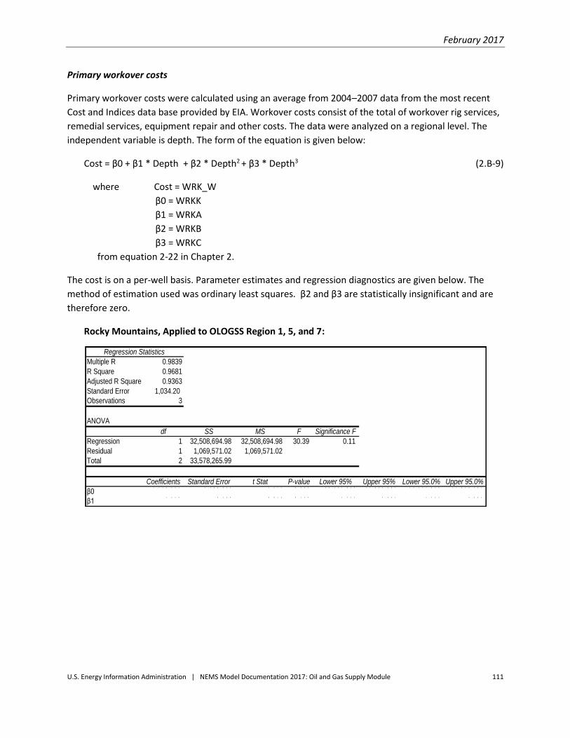
February 2017


Primary workover costs

Primary workover costs were calculated using an average from 2004–2007 data from the most recent

Cost and Indices data base provided by EIA. Workover costs consist of the total of workover rig services,

remedial services, equipment repair and other costs. The data were analyzed on a regional level. The

independent variable is depth. The form of the equation is given below:


where Cost = WRK_W

β0 = WRKK

β1 = WRKA

β2 = WRKB

β3 = WRKC




therefore zero.

Rocky Mountains, Applied to OLOGSS Region 1, 5, and 7:


Multiple R 0.9839

R Square 0.9681



Observations 3

ANOVA


Regression 1 32,508,694.98 32,508,694.98 30.39 0.11

Residual 1 1,069,571.02 1,069,571.02

Total 2 33,578,265.99


β01 , 7 3 6 . 0 8 1 1 , 2 6 6 . 6 3 2 1 . 3 7 1 0 . 4 0 1 - 1 4 , 3 5 7 . 9 3 5 1 7 , 8 3 0 . 0 9 7 - 1 4 , 3 5 7 . 9 3 5 1 7 , 8 3 0 . 0 9 7

β11 . 3 2 0 0 . 2 3 9 5 . 5 1 3 0 . 1 1 4 - 1 . 7 2 2 4 . 3 6 1 - 1 . 7 2 2 4 . 3 6 1

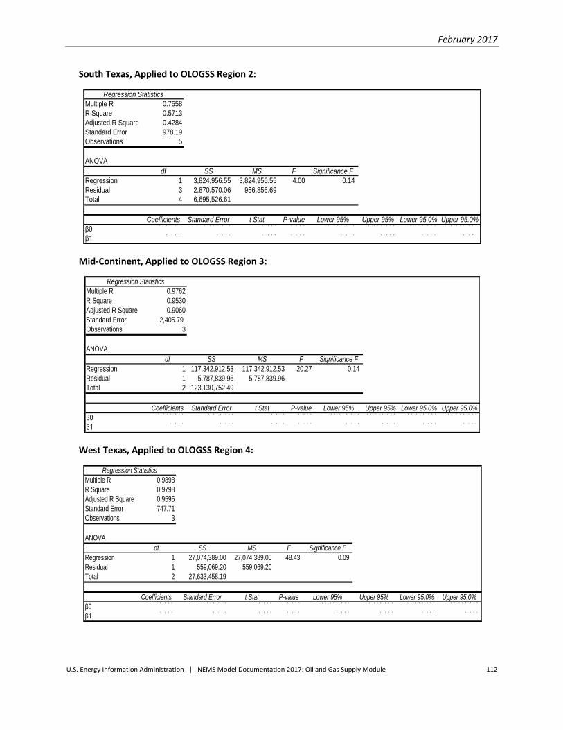
February 2017


South Texas, Applied to OLOGSS Region 2:


West Texas, Applied to OLOGSS Region 4:


Multiple R 0.7558

R Square 0.5713



Observations 5

ANOVA


Regression 1 3,824,956.55 3,824,956.55 4.00 0.14

Residual 3 2,870,570.06 956,856.69

Total 4 6,695,526.61


β01 , 9 4 9 . 4 7 9 1 , 0 4 3 . 9 1 3 1 . 8 6 7 0 . 1 5 9 - 1 , 3 7 2 . 7 2 0 5 , 2 7 1 . 6 7 8 - 1 , 3 7 2 . 7 2 0 5 , 2 7 1 . 6 7 8

β10 . 3 6 4 0 . 1 8 2 1 . 9 9 9 0 . 1 3 9 - 0 . 2 1 6 0 . 9 4 5 - 0 . 2 1 6 0 . 9 4 5


Multiple R 0.9762

R Square 0.9530



Observations 3

ANOVA


Regression 1 117,342,912.53 117,342,912.53 20.27 0.14

Residual 1 5,787,839.96 5,787,839.96

Total 2 123,130,752.49


β0- 2 , 7 3 8 . 0 5 1 2 , 9 4 6 . 4 8 3 - 0 . 9 2 9 0 . 5 2 3 - 4 0 , 1 7 6 . 5 0 2 3 4 , 7 0 0 . 4 0 0 - 4 0 , 1 7 6 . 5 0 2 3 4 , 7 0 0 . 4 0 0

β12 . 5 0 7 0 . 5 5 7 4 . 5 0 3 0 . 1 3 9 - 4 . 5 6 8 9 . 5 8 2 - 4 . 5 6 8 9 . 5 8 2


Multiple R 0.9898

R Square 0.9798



Observations 3

ANOVA


Regression 1 27,074,389.00 27,074,389.00 48.43 0.09

Residual 1 559,069.20 559,069.20

Total 2 27,633,458.19


β03 8 9 . 8 2 1 9 1 5 . 7 5 3 0 . 4 2 6 0 . 7 4 4 - 1 1 , 2 4 5 . 8 7 6 1 2 , 0 2 5 . 5 1 8 - 1 1 , 2 4 5 . 8 7 6 1 2 , 0 2 5 . 5 1 8

β11 . 2 0 4 0 . 1 7 3 6 . 9 5 9 0 . 0 9 1 - 0 . 9 9 5 3 . 4 0 3 - 0 . 9 9 5 3 . 4 0 3

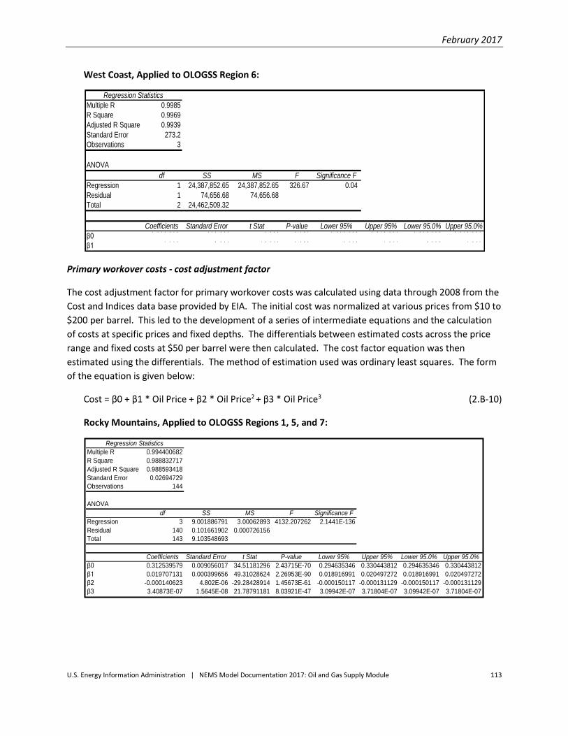
February 2017


West Coast, Applied to OLOGSS Region 6:

Primary workover costs - cost adjustment factor

The cost adjustment factor for primary workover costs was calculated using data through 2008 from the

Cost and Indices data base provided by EIA. The initial cost was normalized at various prices from $10 to

$200 per barrel. This led to the development of a series of intermediate equations and the calculation

of costs at specific prices and fixed depths. The differentials between estimated costs across the price

range and fixed costs at $50 per barrel were then calculated. The cost factor equation was then

estimated using the differentials. The method of estimation used was ordinary least squares. The form

of the equation is given below:




Multiple R 0.9985

R Square 0.9969



Observations 3

ANOVA


Regression 1 24,387,852.65 24,387,852.65 326.67 0.04

Residual 1 74,656.68 74,656.68

Total 2 24,462,509.32


β01 , 3 2 6 . 6 4 8 3 3 4 . 6 4 2 3 . 9 6 4 0 . 1 5 7 - 2 , 9 2 5 . 3 5 9 5 , 5 7 8 . 6 5 4 - 2 , 9 2 5 . 3 5 9 5 , 5 7 8 . 6 5 4

β11 . 1 4 3 0 . 0 6 3 1 8 . 0 7 4 0 . 0 3 5 0 . 3 3 9 1 . 9 4 7 0 . 3 3 9 1 . 9 4 7



R Square 0.988832717



Observations 144

ANOVA


Regression 3 9.001886791 3.00062893 4132.207262 2.1441E-136

Residual 140 0.101661902 0.000726156

Total 143 9.103548693


β0 0.312539579 0.009056017 34.51181296 2.43715E-70 0.294635346 0.330443812 0.294635346 0.330443812

β1 0.019707131 0.000399656 49.31028624 2.26953E-90 0.018916991 0.020497272 0.018916991 0.020497272

β2 -0.000140623 4.802E-06 -29.28428914 1.45673E-61 -0.000150117 -0.000131129 -0.000150117 -0.000131129

β3 3.40873E-07 1.5645E-08 21.78791181 8.03921E-47 3.09942E-07 3.71804E-07 3.09942E-07 3.71804E-07

February 2017







R Square 0.98896985



Observations 144

ANOVA


Regression 3 8.861572267 2.953857422 4184.161269 9.0291E-137

Residual 140 0.098834632 0.000705962

Total 143 8.960406899


β0 0.315903453 0.008929203 35.37868321 1.07799E-71 0.298249938 0.333556967 0.298249938 0.333556967

β1 0.019629392 0.000394059 49.81332121 5.91373E-91 0.018850316 0.020408468 0.018850316 0.020408468

β2 -0.000140391 4.73475E-06 -29.65123432 3.24065E-62 -0.000149752 -0.00013103 -0.000149752 -0.00013103

β3 3.40702E-07 1.5426E-08 22.08625878 1.83379E-47 3.10204E-07 3.712E-07 3.10204E-07 3.712E-07



R Square 0.988994155



Observations 144

ANOVA


Regression 3 9.003736634 3.001245545 4193.504662 7.7373E-137

Residual 140 0.100196473 0.000715689

Total 143 9.103933107


β0 0.312750341 0.00899051 34.78671677 9.00562E-71 0.294975619 0.330525063 0.294975619 0.330525063

β1 0.019699787 0.000396765 49.6510621 9.11345E-91 0.018915362 0.020484212 0.018915362 0.020484212

β2 -0.000140541 4.76726E-06 -29.480463 6.51147E-62 -0.000149966 -0.000131116 -0.000149966 -0.000131116

β3 3.40661E-07 1.55319E-08 21.93302302 3.91217E-47 3.09954E-07 3.71368E-07 3.09954E-07 3.71368E-07



R Square 0.902441789



Observations 144

ANOVA


Regression 3 10.63829925 3.546099748 431.6802228 1.59892E-70

Residual 140 1.150050289 0.008214645

Total 143 11.78834953


β0 0.281549378 0.030459064 9.243533578 3.55063E-16 0.221330174 0.341768582 0.221330174 0.341768582

β1 0.020360006 0.001344204 15.14651492 2.70699E-31 0.017702443 0.02301757 0.017702443 0.02301757

β2 -0.000140998 1.61511E-05 -8.729925387 6.86299E-15 -0.000172929 -0.000109066 -0.000172929 -0.000109066

β3 3.36972E-07 5.26206E-08 6.403797584 2.14112E-09 2.32938E-07 4.41006E-07 2.32938E-07 4.41006E-07

February 2017



Cost to convert a primary to secondary well

The cost to convert a primary to secondary well was calculated using an average from 2004-2007 data

from the most recent Cost and Indices data base provided by EIA. Conversion costs for a primary to a

secondary well consist of pumping equipment, rods and pumps, and supply wells. The data was analyzed

on a regional level. The secondary operations costs for each region are determined by multiplying the

costs in West Texas by the ratio of primary operating costs. This method was used in the National

Petroleum Council’s (NPC) EOR study of 1984. The independent variable is depth. The form of the

equation is given below:


where Cost = PSW_W

β0 = PSWK

β1 = PSWA

β2 = PSWB

β3 = PSWC




therefore zero.



R Square 0.988797046



Observations 144

ANOVA


Regression 3 8.828330392 2.942776797 4118.9013 2.6803E-136

Residual 140 0.100023944 0.000714457

Total 143 8.928354335


β0 0.316566704 0.008982767 35.24155917 1.75819E-71 0.298807292 0.334326116 0.298807292 0.334326116

β1 0.019613748 0.000396423 49.47682536 1.45204E-90 0.018829998 0.020397497 0.018829998 0.020397497

β2 -0.000140368 4.76315E-06 -29.46957335 6.80842E-62 -0.000149785 -0.000130951 -0.000149785 -0.000130951

β3 3.40752E-07 1.55185E-08 21.95777375 3.46083E-47 3.10071E-07 3.71433E-07 3.10071E-07 3.71433E-07

February 2017






Multiple R 0.999208

R Square 0.998416



Observations 3

ANOVA


Regression 1 62,643,414,406.49 62,643,414,406.49 630.34 0.03

Residual 1 99,380,639.94 99,380,639.94

Total 2 62,742,795,046.43


β0- 1 1 5 . 5 5 7 1 2 , 2 0 9 . 4 6 2 - 0 . 0 0 9 0 . 9 9 4 - 1 5 5 , 2 5 0 . 8 1 5 1 5 5 , 0 1 9 . 7 0 1 - 1 5 5 , 2 5 0 . 8 1 5 1 5 5 , 0 1 9 . 7 0 1

β15 7 . 9 3 0 2 . 3 0 7 2 5 . 1 0 7 0 . 0 2 5 2 8 . 6 1 2 8 7 . 2 4 8 2 8 . 6 1 2 8 7 . 2 4 8

0

200000

400000

0 20 40 60 80 100


Multiple R 0.996760

R Square 0.993531



Observations 6

ANOVA


Regression 1 175,651,490,230.16 175,651,490,230.16 614.35 0.00

Residual 4 1,143,664,392.16 285,916,098.04

Total 5 176,795,154,622.33


β0- 1 0 , 7 3 3 . 7 1 4 , 6 4 3 . 6 7 0 - 0 . 7 3 3 0 . 5 0 4 - 5 1 , 3 9 1 . 1 6 9 2 9 , 9 2 3 . 6 9 2 - 5 1 , 3 9 1 . 1 6 9 2 9 , 9 2 3 . 6 9 2

β16 8 . 5 9 3 2 . 7 6 7 2 4 . 7 8 6 0 . 0 0 0 6 0 . 9 0 9 7 6 . 2 7 6 6 0 . 9 0 9 7 6 . 2 7 6


Multiple R 0.999830

R Square 0.999660



Observations 3

ANOVA


Regression 1 48,164,743,341 48,164,743,341 2,939.86 0.01

Residual 1 16,383,350 16,383,350

Total 2 48,181,126,691


β0- 3 2 , 9 1 9 . 3 4 , 9 5 7 . 3 2 0 - 6 . 6 4 1 0 . 0 9 5 - 9 5 , 9 0 7 . 7 6 8 3 0 , 0 6 9 . 1 4 8 - 9 5 , 9 0 7 . 7 6 8 3 0 , 0 6 9 . 1 4 8

β15 0 . 7 9 6 0 . 9 3 7 5 4 . 2 2 0 0 . 0 1 2 3 8 . 8 9 3 6 2 . 7 0 0 3 8 . 8 9 3 6 2 . 7 0 0

0

100000

200000

0 20 40 60 80 100

February 2017




Cost to convert a primary to secondary well - cost adjustment factor

The cost adjustment factor for the cost to convert a primary to secondary well was calculated using data

through 2008 from the Cost and Indices data base provided by EIA. The initial cost was normalized at

various prices from $10 to $200 per barrel. This led to the development of a series of intermediate

equations and the calculation of costs at specific prices and fixed depths. The differentials between

estimated costs across the price range and fixed costs at $50 per barrel were then calculated. The cost

factor equation was then estimated using the differentials. The method of estimation used was ordinary

least squares. The form of the equation is given below:



Multiple R 1.00000

R Square 0.99999



Observations 3

ANOVA


Regression 1 44,056,261,873.48 44,056,261,873.48 144,469.3 0.00

Residual 1 304,952.52 304,952.52

Total 2 44,056,566,825.99


β0- 2 5 , 1 7 5 . 8 6 7 6 . 3 3 5 - 3 7 . 2 2 4 0 . 0 1 7 - 3 3 , 7 6 9 . 3 8 9 - 1 6 , 5 8 2 . 1 6 6 - 3 3 , 7 6 9 . 3 8 9 - 1 6 , 5 8 2 . 1 6 6

β14 8 . 5 8 1 0 . 1 2 8 3 8 0 . 0 9 1 0 . 0 0 2 4 6 . 9 5 7 5 0 . 2 0 5 4 6 . 9 5 7 5 0 . 2 0 5


Multiple R 0.999970

R Square 0.999941



Observations 3

ANOVA


Regression 1 90,641,249,203.56 90,641,249,203.56 16,883.5 0.00

Residual 1 5,368,613.99 5,368,613.99

Total 2 90,646,617,817.55


β0- 4 7 , 7 7 5 . 5 2 , 8 3 7 . 7 6 7 - 1 6 . 8 3 6 0 . 0 3 8 - 8 3 , 8 3 2 . 5 9 7 - 1 1 , 7 1 8 . 4 1 2 - 8 3 , 8 3 2 . 5 9 7 - 1 1 , 7 1 8 . 4 1 2

β16 9 . 6 8 3 0 . 5 3 6 1 2 9 . 9 3 7 0 . 0 0 5 6 2 . 8 6 9 7 6 . 4 9 8 6 2 . 8 6 9 7 6 . 4 9 8

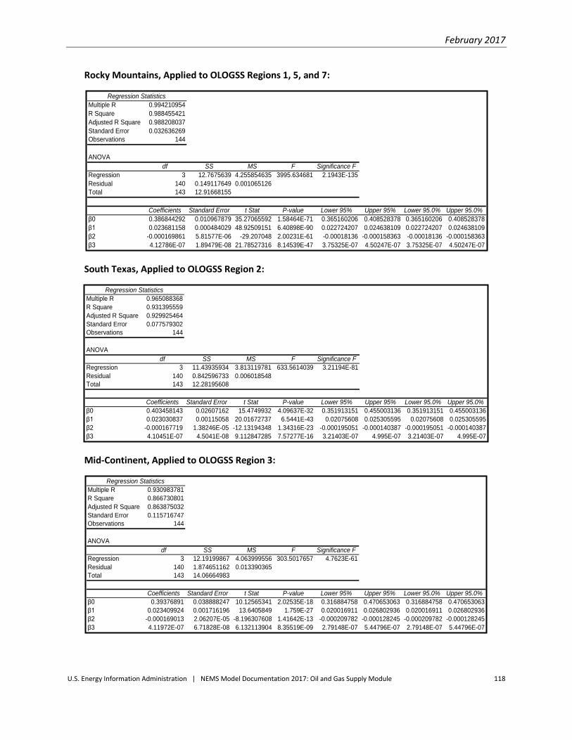
February 2017







R Square 0.988455421



Observations 144

ANOVA


Regression 3 12.7675639 4.255854635 3995.634681 2.1943E-135

Residual 140 0.149117649 0.001065126

Total 143 12.91668155


β0 0.386844292 0.010967879 35.27065592 1.58464E-71 0.365160206 0.408528378 0.365160206 0.408528378

β1 0.023681158 0.000484029 48.92509151 6.40898E-90 0.022724207 0.024638109 0.022724207 0.024638109

β2 -0.000169861 5.81577E-06 -29.207048 2.00231E-61 -0.00018136 -0.000158363 -0.00018136 -0.000158363

β3 4.12786E-07 1.89479E-08 21.78527316 8.14539E-47 3.75325E-07 4.50247E-07 3.75325E-07 4.50247E-07



R Square 0.931395559



Observations 144

ANOVA


Regression 3 11.43935934 3.813119781 633.5614039 3.21194E-81

Residual 140 0.842596733 0.006018548

Total 143 12.28195608


β0 0.403458143 0.02607162 15.4749932 4.09637E-32 0.351913151 0.455003136 0.351913151 0.455003136

β1 0.023030837 0.00115058 20.01672737 6.5441E-43 0.02075608 0.025305595 0.02075608 0.025305595

β2 -0.000167719 1.38246E-05 -12.13194348 1.34316E-23 -0.000195051 -0.000140387 -0.000195051 -0.000140387

β3 4.10451E-07 4.5041E-08 9.112847285 7.57277E-16 3.21403E-07 4.995E-07 3.21403E-07 4.995E-07



R Square 0.866730801



Observations 144

ANOVA


Regression 3 12.19199867 4.063999556 303.5017657 4.7623E-61

Residual 140 1.874651162 0.013390365

Total 143 14.06664983


β0 0.39376891 0.038888247 10.12565341 2.02535E-18 0.316884758 0.470653063 0.316884758 0.470653063

β1 0.023409924 0.001716196 13.6405849 1.759E-27 0.020016911 0.026802936 0.020016911 0.026802936

β2 -0.000169013 2.06207E-05 -8.196307608 1.41642E-13 -0.000209782 -0.000128245 -0.000209782 -0.000128245

β3 4.11972E-07 6.71828E-08 6.132113904 8.35519E-09 2.79148E-07 5.44796E-07 2.79148E-07 5.44796E-07

February 2017




Cost to convert a producer to an injector

The cost to convert a production well to an injection well was calculated using an average from 2004–

2007 data from the most recent Cost and Indices data base provided by EIA. Conversion costs for a

production to an injection well consist of tubing replacement, distribution lines and header costs. The

data was analyzed on a regional level. The secondary operation costs for each region are determined by

multiplying the costs in West Texas by the ratio of primary operating costs. This method was used in the

NPC EOR study of 1984. The independent variable is depth. The form of the equation is given below:



R Square 0.866060752



Observations 144

ANOVA


Regression 3 12.5418858 4.180628599 301.7500036 6.76263E-61

Residual 140 1.939645392 0.01385461

Total 143 14.48153119


β0 0.363067907 0.039556632 9.178433366 5.17966E-16 0.284862323 0.441273492 0.284862323 0.441273492

β1 0.024133277 0.001745693 13.82446554 5.96478E-28 0.020681947 0.027584606 0.020681947 0.027584606

β2 -0.000175479 2.09751E-05 -8.366057262 5.44112E-14 -0.000216948 -0.00013401 -0.000216948 -0.00013401

β3 4.28328E-07 6.83375E-08 6.267838182 4.24825E-09 2.93221E-07 5.63435E-07 2.93221E-07 5.63435E-07



R Square 0.865248054



Observations 144

ANOVA


Regression 3 12.19426209 4.06475403 299.6486777 1.03233E-60

Residual 140 1.899109212 0.013565066

Total 143 14.0933713


β0 0.393797507 0.039141107 10.06097011 2.96602E-18 0.316413437 0.471181577 0.316413437 0.471181577

β1 0.023409194 0.001727356 13.55204156 2.96327E-27 0.01999412 0.026824269 0.01999412 0.026824269

β2 -0.000168995 2.07548E-05 -8.142483197 1.91588E-13 -0.000210029 -0.000127962 -0.000210029 -0.000127962

β3 4.11911E-07 6.76196E-08 6.091589926 1.02095E-08 2.78223E-07 5.45599E-07 2.78223E-07 5.45599E-07

February 2017



where Cost = PSI_W

β0 = PSIK

β1 = PSIA

β2 = PSIB

β3 = PSIC




therefore zero.

West Texas, applied to OLOGSS region 4:

South Texas, applied to OLOGSS region 2:


Multiple R 0.994714

R Square 0.989456



Observations 3

ANOVA


Regression 1 963,939,802.16 963,939,802.16 93.84 0.07

Residual 1 10,271,635.04 10,271,635.04

Total 2 974,211,437.20

Coefficients Standard Error t Stat P-value Lower 95% Upper 95% Lower 95.0%Upper 95.0%

β01 1 , 1 2 9 . 3 3 , 9 2 5 . 2 3 3 2 . 8 3 5 0 . 2 1 6 - 3 8 , 7 4 5 . 2 5 9 6 1 , 0 0 3 . 9 3 7 - 3 8 , 7 4 5 . 2 5 9 6 1 , 0 0 3 . 9 3 7

β17 . 1 8 6 0 . 7 4 2 9 . 6 8 7 0 . 0 6 5 - 2 . 2 3 9 1 6 . 6 1 1 - 2 . 2 3 9 1 6 . 6 1 1


Multiple R 0.988716

R Square 0.977560



Observations 6

ANOVA


Regression 1 3,428,080,322.21 3,428,080,322.21 174.25 0.00

Residual 4 78,691,571.93 19,672,892.98

Total 5 3,506,771,894.14


β02 4 , 6 4 0 . 6 3 , 8 4 1 . 1 8 1 6 . 4 1 5 0 . 0 0 3 1 3 , 9 7 5 . 7 6 3 3 5 , 3 0 5 . 4 6 2 1 3 , 9 7 5 . 7 6 3 3 5 , 3 0 5 . 4 6 2

β19 . 5 8 2 0 . 7 2 6 1 3 . 2 0 1 0 . 0 0 0 7 . 5 6 7 1 1 . 5 9 8 7 . 5 6 7 1 1 . 5 9 8

February 2017




West Coast, applied to OLOGSS region 6:


Multiple R 0.993556

R Square 0.987154



Observations 3

ANOVA


Regression 1 1,092,230,257.01 1,092,230,257.01 76.84 0.07

Residual 1 14,213,917.83 14,213,917.83

Total 2 1,106,444,174.85


β09 , 3 5 6 . 4 1 1 4 , 6 1 7 . 4 5 3 2 . 0 2 6 0 . 2 9 2 - 4 9 , 3 1 3 . 6 4 8 6 8 , 0 2 6 . 4 6 9 - 4 9 , 3 1 3 . 6 4 8 6 8 , 0 2 6 . 4 6 9

β17 . 6 4 9 0 . 8 7 3 8 . 7 6 6 0 . 0 7 2 - 3 . 4 3 8 1 8 . 7 3 7 - 3 . 4 3 8 1 8 . 7 3 7

0

50000

100000

0 20 40 60 80 100


Multiple R 0.995436

R Square 0.990893



Observations 3

ANOVA


Regression 1 1,160,837,008.65 1,160,837,008.65 108.80 0.06

Residual 1 10,669,310.85 10,669,310.85

Total 2 1,171,506,319.50


β02 4 , 0 5 4 . 3 1 1 4 , 0 0 0 . 4 9 6 6 . 0 1 3 0 . 1 0 5 - 2 6 , 7 7 6 . 5 8 9 7 4 , 8 8 5 . 2 1 1 - 2 6 , 7 7 6 . 5 8 9 7 4 , 8 8 5 . 2 1 1

β17 . 8 8 6 0 . 7 5 6 1 0 . 4 3 1 0 . 0 6 1 - 1 . 7 2 0 1 7 . 4 9 2 - 1 . 7 2 0 1 7 . 4 9 2

0

50000

100000

0 20 40 60 80 100


Multiple R 0.998023

R Square 0.996050



Observations 3

ANOVA


Regression 1 2,125,305,559.02 2,125,305,559.02 252.17 0.04

Residual 1 8,427,914.12 8,427,914.12

Total 2 2,133,733,473.15


β01 1 , 1 2 5 . 8 4 6 3 , 5 5 5 . 5 4 1 3 . 1 2 9 0 . 1 9 7 - 3 4 , 0 5 1 . 3 9 1 5 6 , 3 0 3 . 0 8 3 - 3 4 , 0 5 1 . 3 9 1 5 6 , 3 0 3 . 0 8 3

β11 0 . 6 7 0 0 . 6 7 2 1 5 . 8 8 0 0 . 0 4 0 2 . 1 3 3 1 9 . 2 0 8 2 . 1 3 3 1 9 . 2 0 8

0

50000

100000

0 20 40 60 80 100

February 2017


Cost to convert a producer to an injector - cost adjustment factor

The cost adjustment factor for the cost to convert a producer to an injector was calculated using data












R Square 0.988678308



Observations 144

ANOVA


Regression 3 8.715578807 2.905192936 4075.214275 5.6063E-136

Residual 140 0.099805061 0.000712893

Total 143 8.815383869


β0 0.318906241 0.008972933 35.54091476 6.05506E-72 0.301166271 0.336646211 0.301166271 0.336646211

β1 0.019564167 0.000395989 49.40584281 1.75621E-90 0.018781276 0.020347059 0.018781276 0.020347059

β2 -0.000140323 4.75794E-06 -29.49235038 6.20216E-62 -0.00014973 -0.000130916 -0.00014973 -0.000130916

β3 3.40991E-07 1.55015E-08 21.9972576 2.84657E-47 3.10343E-07 3.71638E-07 3.10343E-07 3.71638E-07



R Square 0.989317613



Observations 144

ANOVA


Regression 3 8.678119686 2.892706562 4321.895164 9.5896E-138

Residual 140 0.093704013 0.000669314

Total 143 8.771823699


β0 0.316208692 0.008694352 36.36943685 3.2883E-73 0.299019491 0.333397893 0.299019491 0.333397893

β1 0.01974618 0.000383695 51.46325116 7.80746E-93 0.018987594 0.020504765 0.018987594 0.020504765

β2 -0.000142963 4.61022E-06 -31.00997536 1.39298E-64 -0.000152077 -0.000133848 -0.000152077 -0.000133848

β3 3.4991E-07 1.50202E-08 23.29589312 5.12956E-50 3.20214E-07 3.79606E-07 3.20214E-07 3.79606E-07

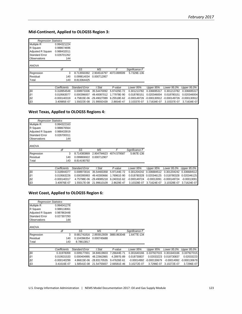
February 2017







R Square 0.988674696



Observations 144

ANOVA


Regression 3 8.713550392 2.904516797 4073.899599 5.7329E-136

Residual 140 0.099814034 0.000712957

Total 143 8.813364425


β0 0.318954549 0.008973336 35.54470092 5.97425E-72 0.301213782 0.336695317 0.301213782 0.336695317

β1 0.019563077 0.000396007 49.40087012 1.77978E-90 0.018780151 0.020346004 0.018780151 0.020346004

β2 -0.000140319 4.75815E-06 -29.49027089 6.25518E-62 -0.000149726 -0.000130912 -0.000149726 -0.000130912

β3 3.40985E-07 1.55022E-08 21.99592439 2.8654E-47 3.10337E-07 3.71634E-07 3.10337E-07 3.71634E-07



R Square 0.988676564



Observations 144

ANOVA


Regression 3 8.714383869 2.904794623 4074.579587 5.667E-136

Residual 140 0.099806922 0.000712907

Total 143 8.814190792


β0 0.318944377 0.008973016 35.54483358 5.97144E-72 0.301204242 0.336684512 0.301204242 0.336684512

β1 0.019563226 0.000395993 49.40300666 1.76961E-90 0.018780328 0.020346125 0.018780328 0.020346125

β2 -0.000140317 4.75798E-06 -29.49085218 6.24031E-62 -0.000149724 -0.00013091 -0.000149724 -0.00013091

β3 3.40976E-07 1.55017E-08 21.99610109 2.8629E-47 3.10328E-07 3.71624E-07 3.10328E-07 3.71624E-07



R Square 0.988118061



Observations 144

ANOVA


Regression 3 8.681741816 2.893913939 3880.863048 1.6477E-134

Residual 140 0.104396354 0.000745688

Total 143 8.78613817


β0 0.31978359 0.009177001 34.84619603 7.26644E-71 0.301640166 0.337927015 0.301640166 0.337927015

β1 0.019531533 0.000404995 48.22662865 4.2897E-89 0.018730837 0.02033223 0.018730837 0.02033223

β2 -0.000140299 4.86615E-06 -28.83170535 9.47626E-61 -0.00014992 -0.000130679 -0.00014992 -0.000130679

β3 3.41616E-07 1.58541E-08 21.54755837 2.66581E-46 3.10272E-07 3.7296E-07 3.10272E-07 3.7296E-07

February 2017


Facilities upgrade costs for crude oil wells

The facilities upgrading cost for secondary oil wells was calculated using an average from 2004–2007

data from the most recent Cost and Indices data base provided by EIA. Facilities costs for a secondary oil

well consist of plant costs and electrical costs. The data were analyzed on a regional level. The secondary

operation costs for each region are determined by multiplying the costs in West Texas by the ratio of

primary operating costs. This method was used in the NPC EOR study of 1984. The independent variable

is depth. The form of the equation is given below:


where Cost = FAC_W

β0 = FACUPK

β1 = FACUPA

β2 = FACUPB

β3 = FACUPC




therefore zero.



Multiple R 0.947660

R Square 0.898060



Observations 3

ANOVA


Regression 1 353,260,332.81 353,260,332.81 8.81 0.21

Residual 1 40,099,063.51 40,099,063.51

Total 2 393,359,396.32


β02 0 , 7 1 1 . 7 6 1 7 , 7 5 5 . 5 5 3 2 . 6 7 1 0 . 2 2 8 - 7 7 , 8 3 1 . 4 5 5 1 1 9 , 2 5 4 . 9 7 7 - 7 7 , 8 3 1 . 4 5 5 1 1 9 , 2 5 4 . 9 7 7

β14 . 3 5 0 1 . 4 6 6 2 . 9 6 8 0 . 2 0 7 - 1 4 . 2 7 3 2 2 . 9 7 3 - 1 4 . 2 7 3 2 2 . 9 7 3

February 2017






Multiple R 0.942744

R Square 0.888767



Observations 5

ANOVA


Regression 1 1,075,905,796.72 1,075,905,796.72 23.97 0.02

Residual 3 134,654,629.89 44,884,876.63

Total 4 1,210,560,426.61


β03 3 , 6 6 5 . 6 7 , 1 4 9 . 7 4 7 4 . 7 0 9 0 . 0 1 8 1 0 , 9 1 1 . 9 2 1 5 6 , 4 1 9 . 3 3 8 1 0 , 9 1 1 . 9 2 1 5 6 , 4 1 9 . 3 3 8

β16 . 1 1 2 1 . 2 4 8 4 . 8 9 6 0 . 0 1 6 2 . 1 3 9 1 0 . 0 8 5 2 . 1 3 9 1 0 . 0 8 5


Multiple R 0.950784

R Square 0.903990



Observations 3

ANOVA


Regression 1 423,335,427.35 423,335,427.35 9.42 0.20

Residual 1 44,961,183.70 44,961,183.70

Total 2 468,296,611.04


β01 9 , 0 3 2 . 5 5 0 8 , 2 1 2 . 2 9 4 2 . 3 1 8 0 . 2 5 9 - 8 5 , 3 1 4 . 0 9 4 1 2 3 , 3 7 9 . 1 9 4 - 8 5 , 3 1 4 . 0 9 4 1 2 3 , 3 7 9 . 1 9 4

β14 . 7 6 2 1 . 5 5 2 3 . 0 6 8 0 . 2 0 1 - 1 4 . 9 5 7 2 4 . 4 8 2 - 1 4 . 9 5 7 2 4 . 4 8 2

0

50000

100000

0 20 40 60 80 100


Multiple R 0.90132

R Square 0.81238


Standard Error 8,531

Observations 3

ANOVA


Regression 1 315,132,483.91 315,132,483.91 4.33 0.29

Residual 1 72,780,134.04 72,780,134.04

Total 2 387,912,617.95


β03 7 , 3 2 2 1 0 , 4 4 8 . 4 5 4 3 . 5 7 2 0 . 1 7 4 - 9 5 , 4 3 7 . 5 8 9 1 7 0 , 0 8 1 . 6 7 7 - 9 5 , 4 3 7 . 5 8 9 1 7 0 , 0 8 1 . 6 7 7

β14 . 1 0 9 1 . 9 7 5 2 . 0 8 1 0 . 2 8 5 - 2 0 . 9 8 0 2 9 . 1 9 8 - 2 0 . 9 8 0 2 9 . 1 9 8

0

50000

100000

0 20 40 60 80 100

February 2017



Facilities upgrade costs for oil wells - cost adjustment factor

The cost adjustment factor for facilities upgrade costs for oil wells was calculated using data through

2008 from the Cost and Indices data base provided by EIA. The initial cost was normalized at various

prices from $10 to $200 per barrel. This led to the development of a series of intermediate equations

and the calculation of costs at specific prices and fixed depths. The differentials between estimated

costs across the price range and fixed costs at $50 per barrel were then calculated. The cost factor

equation was then estimated using the differentials. The method of estimation used was ordinary least

squares. The form of the equation is given below:




Multiple R 0.974616

R Square 0.949876



Observations 3

ANOVA


Regression 1 867,401,274.79 867,401,274.79 18.95 0.14

Residual 1 45,771,551.83 45,771,551.83

Total 2 913,172,826.62


β02 3 , 7 4 6 . 6 8 , 2 8 5 . 9 7 2 2 . 8 6 6 0 . 2 1 4 - 8 1 , 5 3 6 . 2 5 1 1 2 9 , 0 2 9 . 3 5 4 - 8 1 , 5 3 6 . 2 5 1 1 2 9 , 0 2 9 . 3 5 4

β16 . 8 1 7 1 . 5 6 6 4 . 3 5 3 0 . 1 4 4 - 1 3 . 0 8 0 2 6 . 7 1 3 - 1 3 . 0 8 0 2 6 . 7 1 3



R Square 0.988468759



Observations 144

ANOVA


Regression 3 8.615198936 2.871732979 4000.310244 2.0238E-135

Residual 140 0.100502859 0.000717878

Total 143 8.715701795


β0 0.321111529 0.009004246 35.66223488 3.93903E-72 0.303309651 0.338913406 0.303309651 0.338913406

β1 0.019515262 0.000397371 49.11095778 3.88014E-90 0.018729638 0.020300885 0.018729638 0.020300885

β2 -0.00014023 4.77454E-06 -29.37035185 1.02272E-61 -0.00014967 -0.00013079 -0.00014967 -0.00013079

β3 3.4105E-07 1.55556E-08 21.92459665 4.07897E-47 3.10296E-07 3.71805E-07 3.10296E-07 3.71805E-07

February 2017







R Square 0.988468723



Observations 144

ANOVA


Regression 3 8.615504692 2.871834897 4000.297521 2.0242E-135

Residual 140 0.100506746 0.000717905

Total 143 8.716011438


β0 0.321091731 0.00900442 35.65934676 3.9795E-72 0.30328951 0.338893953 0.30328951 0.338893953

β1 0.019515756 0.000397379 49.11125155 3.87707E-90 0.018730117 0.020301395 0.018730117 0.020301395

β2 -0.000140234 4.77464E-06 -29.37065243 1.02145E-61 -0.000149674 -0.000130794 -0.000149674 -0.000130794

β3 3.41061E-07 1.55559E-08 21.92486379 4.07357E-47 3.10306E-07 3.71816E-07 3.10306E-07 3.71816E-07



R Square 0.989788377



Observations 144

ANOVA


Regression 3 8.892246941 2.964082314 4523.289171 4.0903E-139

Residual 140 0.0917411 0.000655294

Total 143 8.983988041


β0 0.305413562 0.008602806 35.50162345 6.96151E-72 0.288405354 0.32242177 0.288405354 0.32242177

β1 0.019922983 0.000379655 52.47659224 5.82045E-94 0.019172385 0.020673581 0.019172385 0.020673581

β2 -0.000143398 4.56168E-06 -31.43544891 2.62249E-65 -0.000152417 -0.00013438 -0.000152417 -0.00013438

β3 3.48664E-07 1.48621E-08 23.45993713 2.3433E-50 3.1928E-07 3.78047E-07 3.1928E-07 3.78047E-07



R Square 0.988470767



Observations 144

ANOVA


Regression 3 8.616820316 2.872273439 4001.015021 1.9993E-135

Residual 140 0.100504067 0.000717886

Total 143 8.717324383


β0 0.32105584 0.0090043 35.65583598 4.02926E-72 0.303253856 0.338857825 0.303253856 0.338857825

β1 0.019516684 0.000397373 49.11424236 3.84594E-90 0.018731056 0.020302312 0.018731056 0.020302312

β2 -0.00014024 4.77457E-06 -29.37236101 1.01431E-61 -0.00014968 -0.000130801 -0.00014968 -0.000130801

β3 3.4108E-07 1.55557E-08 21.92639924 4.0427E-47 3.10326E-07 3.71835E-07 3.10326E-07 3.71835E-07

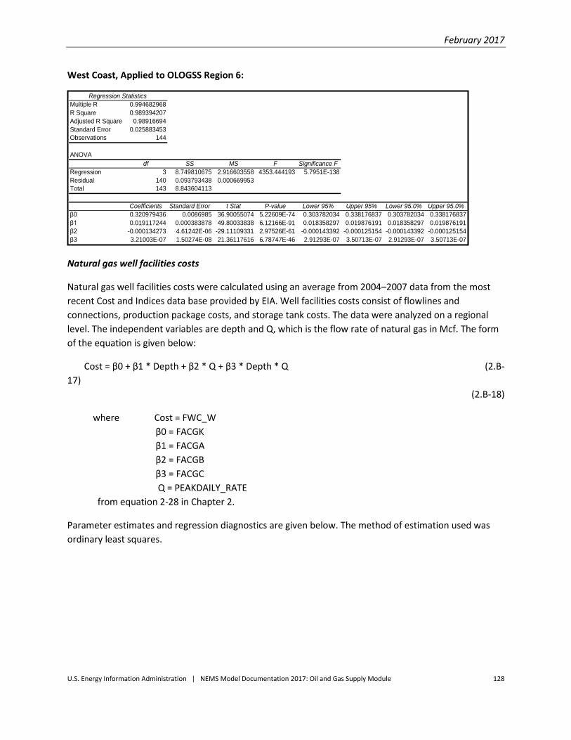
February 2017



Natural gas well facilities costs

Natural gas well facilities costs were calculated using an average from 2004–2007 data from the most

recent Cost and Indices data base provided by EIA. Well facilities costs consist of flowlines and

connections, production package costs, and storage tank costs. The data were analyzed on a regional

level. The independent variables are depth and Q, which is the flow rate of natural gas in Mcf. The form


Cost = β0 + β1 * Depth + β2 * Q + β3 * Depth * Q (2.B-

17)

(2.B-18)

where Cost = FWC_W

β0 = FACGK

β1 = FACGA

β2 = FACGB

β3 = FACGC

Q = PEAKDAILY_RATE


Parameter estimates and regression diagnostics are given below. The method of estimation used was

ordinary least squares.



R Square 0.989394207



Observations 144

ANOVA


Regression 3 8.749810675 2.916603558 4353.444193 5.7951E-138

Residual 140 0.093793438 0.000669953

Total 143 8.843604113


β0 0.320979436 0.0086985 36.90055074 5.22609E-74 0.303782034 0.338176837 0.303782034 0.338176837

β1 0.019117244 0.000383878 49.80033838 6.12166E-91 0.018358297 0.019876191 0.018358297 0.019876191

β2 -0.000134273 4.61242E-06 -29.11109331 2.97526E-61 -0.000143392 -0.000125154 -0.000143392 -0.000125154

β3 3.21003E-07 1.50274E-08 21.36117616 6.78747E-46 2.91293E-07 3.50713E-07 2.91293E-07 3.50713E-07

February 2017




Mid-Continent, applied to OLOGSS regions 3 and 6:


Multiple R 0.9834

R Square 0.9672



Observations 13

ANOVA


Regression 3 8,982,542,532.41 2,994,180,844.14 88.39 0.00

Residual 9 304,879,039.45 33,875,448.83

Total 12 9,287,421,571.86


β03 , 4 7 7 . 4 1 4 , 6 9 4 . 0 3 0 . 7 4 0 . 4 8 - 7 , 1 4 1 . 2 4 1 4 , 0 9 6 . 0 5 - 7 , 1 4 1 . 2 4 1 4 , 0 9 6 . 0 5

β 1 5 . 0 4 0 . 4 0 1 2 . 5 1 0 . 0 0 4 . 1 3 5 . 9 5 4 . 1 3 5 . 9 5

β 2 6 3 . 8 7 1 9 . 0 7 3 . 3 5 0 . 0 1 2 0 . 7 2 1 0 7 . 0 2 2 0 . 7 2 1 0 7 . 0 2

β30 . 0 0 0 . 0 0 - 3 . 1 8 0 . 0 1 - 0 . 0 1 0 . 0 0 - 0 . 0 1 0 . 0 0


Multiple R 0.9621

R Square 0.9256



Observations 23

ANOVA


Regression 3 16,213,052,116.02 5,404,350,705.34 78.84 0.00

Residual 19 1,302,484,315.70 68,551,806.09

Total 22 17,515,536,431.72


β01 4 , 9 6 0 . 6 0 4 , 0 6 6 . 9 8 3 . 6 8 0 . 0 0 6 , 4 4 8 . 3 1 2 3 , 4 7 2 . 9 0 6 , 4 4 8 . 3 1 2 3 , 4 7 2 . 9 0

β 1 4 . 8 7 0 . 4 7 1 0 . 3 4 0 . 0 0 3 . 8 8 5 . 8 5 3 . 8 8 5 . 8 5

β 2 2 8 . 4 9 6 . 4 2 4 . 4 3 0 . 0 0 1 5 . 0 4 4 1 . 9 3 1 5 . 0 4 4 1 . 9 3

β30 . 0 0 0 . 0 0 - 3 . 6 2 0 . 0 0 0 . 0 0 0 . 0 0 0 . 0 0 0 . 0 0


Multiple R 0.9917

R Square 0.9835



Observations 11

ANOVA


Regression 3 6,796,663,629.62 2,265,554,543.21 139.47 0.00

Residual 7 113,710,456.60 16,244,350.94

Total 10 6,910,374,086.22


β01 0 , 1 8 5 . 9 2 3 , 4 4 1 . 4 1 2 . 9 6 0 . 0 2 2 , 0 4 8 . 2 9 1 8 , 3 2 3 . 5 4 2 , 0 4 8 . 2 9 1 8 , 3 2 3 . 5 4

β 1 4 . 5 1 0 . 2 9 1 5 . 7 1 0 . 0 0 3 . 8 3 5 . 1 8 3 . 8 3 5 . 1 8

β 2 5 5 . 3 8 1 4 . 0 5 3 . 9 4 0 . 0 1 2 2 . 1 6 8 8 . 6 0 2 2 . 1 6 8 8 . 6 0

β30 . 0 0 0 . 0 0 - 3 . 7 8 0 . 0 1 - 0 . 0 1 0 . 0 0 - 0 . 0 1 0 . 0 0

February 2017



Gas well facilities costs - cost adjustment factor

The cost adjustment factor for gas well facilities cost was calculated using data through 2008 from the

Cost and Indices data base provided by EIA. The initial cost was normalized at various prices from $1 to

$20 per Mcf. This led to the development of a series of intermediate equations and the calculation of

costs at specific prices and fixed depths. The differentials between estimated costs across the price

range and fixed costs at $5 per Mcf were then calculated. The cost factor equation was then estimated

using the differentials. The form of the equation is given below:




Multiple R 0.9594

R Square 0.9204



Observations 10

ANOVA


Regression 3 4,322,988,996.06 1,440,996,332.02 23.12 0.00

Residual 6 373,981,660.54 62,330,276.76

Total 9 4,696,970,656.60


β07 , 9 2 2 . 4 8 8 , 2 0 0 . 0 6 0 . 9 7 0 . 3 7 - 1 2 , 1 4 2 . 3 6 2 7 , 9 8 7 . 3 1 - 1 2 , 1 4 2 . 3 6 2 7 , 9 8 7 . 3 1

β 1 6 . 5 1 1 . 1 4 5 . 7 1 0 . 0 0 3 . 7 2 9 . 3 0 3 . 7 2 9 . 3 0

β 2 8 9 . 2 6 2 8 . 8 8 3 . 0 9 0 . 0 2 1 8 . 5 9 1 5 9 . 9 4 1 8 . 5 9 1 5 9 . 9 4

β3- 0 . 0 1 0 . 0 0 - 2 . 7 7 0 . 0 3 - 0 . 0 1 0 . 0 0 - 0 . 0 1 0 . 0 0



R Square 0.991485789



Observations 144

ANOVA


Regression 3 10.3648558 3.454951933 5434.365566 1.2179E-144

Residual 140 0.089006392 0.00063576

Total 143 10.45386219


β0 0.276309237 0.008473615 32.60818851 2.86747E-67 0.259556445 0.293062029 0.259556445 0.293062029

β1 0.20599743 0.003739533 55.08640551 8.89871E-97 0.198604173 0.213390688 0.198604173 0.213390688

β2 -0.014457925 0.000449317 -32.17753015 1.48375E-66 -0.015346249 -0.0135696 -0.015346249 -0.0135696

β3 0.000347281 1.46389E-05 23.72318475 6.71084E-51 0.000318339 0.000376223 0.000318339 0.000376223

February 2017



Mid-Continent, Applied to OLOGSS Regions 3 and 6:




R Square 0.991052684



Observations 144

ANOVA


Regression 3 10.22936837 3.409789455 5169.05027 3.9254E-143

Residual 140 0.092351689 0.000659655

Total 143 10.32172006


β0 0.280854163 0.008631386 32.5387085 3.73403E-67 0.263789449 0.297918878 0.263789449 0.297918878

β1 0.204879431 0.00380916 53.78599024 2.17161E-95 0.197348518 0.212410345 0.197348518 0.212410345

β2 -0.014391989 0.000457683 -31.44530093 2.52353E-65 -0.015296854 -0.013487125 -0.015296854 -0.013487125

β3 0.000345909 1.49115E-05 23.19753012 8.21832E-50 0.000316428 0.00037539 0.000316428 0.00037539



R Square 0.991042698



Observations 144

ANOVA


Regression 3 10.22356717 3.407855722 5163.235345 4.2442E-143

Residual 140 0.092403264 0.000660023

Total 143 10.31597043


β0 0.280965064 0.008633796 32.5424714 3.68097E-67 0.263895586 0.298034543 0.263895586 0.298034543

β1 0.204856879 0.003810223 53.7650588 2.28751E-95 0.197323863 0.212389895 0.197323863 0.212389895

β2 -0.014391983 0.000457811 -31.43650889 2.61165E-65 -0.0152971 -0.013486865 -0.0152971 -0.013486865

β3 0.000345929 1.49156E-05 23.19242282 8.42221E-50 0.00031644 0.000375418 0.00031644 0.000375418



R Square 0.990926606



Observations 144

ANOVA


Regression 3 10.15228252 3.384094173 5096.576002 1.0453E-142

Residual 140 0.092959113 0.000663994

Total 143 10.24524163


β0 0.282511839 0.008659725 32.62364879 2.704E-67 0.265391097 0.299632581 0.265391097 0.299632581

β1 0.204502598 0.003821666 53.51137044 4.3021E-95 0.196946958 0.212058237 0.196946958 0.212058237

β2 -0.014382652 0.000459186 -31.32206064 4.08566E-65 -0.015290487 -0.013474816 -0.015290487 -0.013474816

β3 0.000345898 1.49604E-05 23.12086258 1.18766E-49 0.00031632 0.000375475 0.00031632 0.000375475

February 2017


Fixed annual costs for crude oil wells

The fixed annual cost for crude oil wells was calculated using an average from 2004–2007 data from the

most recent Cost and Indices data base provided by EIA. Fixed annual costs consist of supervision and

overhead costs, auto usage costs, operative supplies, labor costs, supplies and services costs, equipment

usage and other costs. The data were analyzed on a regional level. The independent variable is depth.

The form of the equation is given below:


where Cost = OMO_W

β0 = OMOK

β1 = OMOA

β2 = OMOB

β3 = OMOC




therefore zero.



Multiple R 0.9895

R Square 0.9792



Observations 3

ANOVA


Regression 1 1,290,021.8 1,290,021.8 47.0 0.1

Residual 1 27,419.5 27,419.5

Total 2 1,317,441.3


β06 , 0 2 6 . 9 4 9 2 0 2 . 8 0 4 2 9 . 7 1 8 0 . 0 2 1 3 , 4 5 0 . 0 9 7 8 , 6 0 3 . 8 0 2 3 , 4 5 0 . 0 9 7 8 , 6 0 3 . 8 0 2

β10 . 2 6 3 0 . 0 3 8 6 . 8 5 9 0 . 0 9 2 - 0 . 2 2 4 0 . 7 5 0 - 0 . 2 2 4 0 . 7 5 0

February 2017






Multiple R 0.8631

R Square 0.7449



Observations 6

ANOVA


Regression 1 88,902,026.9 88,902,026.9 11.7 0.0

Residual 4 30,452,068.1 7,613,017.0

Total 5 119,354,095.0


β07 , 1 7 1 . 3 5 8 2 , 3 8 9 . 5 1 1 3 . 0 0 1 0 . 0 4 0 5 3 6 . 9 9 8 1 3 , 8 0 5 . 7 1 8 5 3 6 . 9 9 8 1 3 , 8 0 5 . 7 1 8

β11 . 5 4 3 0 . 4 5 2 3 . 4 1 7 0 . 0 2 7 0 . 2 8 9 2 . 7 9 7 0 . 2 8 9 2 . 7 9 7


Multiple R 0.9888

R Square 0.9777



Observations 3

ANOVA


Regression 1 4,654,650.4 4,654,650.4 43.9 0.1

Residual 1 106,147.3 106,147.3

Total 2 4,760,797.7


β05 , 5 7 2 . 2 8 3 3 9 9 . 0 2 5 1 3 . 9 6 5 0 . 0 4 6 5 0 2 . 2 1 1 1 0 , 6 4 2 . 3 5 5 5 0 2 . 2 1 1 1 0 , 6 4 2 . 3 5 5

β10 . 4 9 9 0 . 0 7 5 6 . 6 2 2 0 . 0 9 5 - 0 . 4 5 9 1 . 4 5 8 - 0 . 4 5 9 1 . 4 5 8


Multiple R 0.9634

R Square 0.9282



Observations 4

ANOVA


Regression 1 5,368,949.5 5,368,949.5 25.9 0.0

Residual 2 415,138.5 207,569.2

Total 3 5,784,088.0


β06 , 3 2 7 . 7 3 3 4 4 7 . 8 0 9 1 4 . 1 3 0 0 . 0 0 5 4 , 4 0 0 . 9 6 4 8 , 2 5 4 . 5 0 1 4 , 4 0 0 . 9 6 4 8 , 2 5 4 . 5 0 1

β10 . 3 0 2 0 . 0 5 9 5 . 0 8 6 0 . 0 3 7 0 . 0 4 6 0 . 5 5 7 0 . 0 4 6 0 . 5 5 7

February 2017



Fixed annual costs for oil wells - cost adjustment factor

The cost adjustment factor of the fixed annual cost for oil wells was calculated using data through 2008

from the Cost and Indices data base provided by EIA. The initial cost was normalized at various prices

from $10 to $200 per barrel. This led to the development of a series of intermediate equations and the

calculation of costs at specific prices and fixed depths. The differentials between estimated costs across

the price range and fixed costs at $50 per barrel were then calculated. The cost factor equation was

then estimated using the differentials. The method of estimation used was ordinary least squares. The

form of the equation is given below:




Multiple R 0.9908

R Square 0.9817



Observations 4

ANOVA


Regression 1 10,498,366.6 10,498,366.6 107.1 0.0

Residual 2 196,056.3 98,028.2

Total 3 10,694,422.9


β05 , 1 9 3 . 3 9 9 3 0 7 . 7 4 2 1 6 . 8 7 6 0 . 0 0 3 3 , 8 6 9 . 2 9 1 6 , 5 1 7 . 5 0 8 3 , 8 6 9 . 2 9 1 6 , 5 1 7 . 5 0 8

β10 . 4 2 2 0 . 0 4 1 1 0 . 3 4 9 0 . 0 0 9 0 . 2 4 6 0 . 5 9 7 0 . 2 4 6 0 . 5 9 7



R Square 0.988064394



Observations 144

ANOVA


Regression 3 8.424110153 2.808036718 3863.203308 2.2587E-134

Residual 140 0.101761442 0.000726867

Total 143 8.525871595


β0 0.325522735 0.00906045 35.9278779 1.54278E-72 0.30760974 0.343435731 0.30760974 0.343435731

β1 0.019415379 0.000399851 48.55651174 1.74247E-89 0.018624852 0.020205906 0.018624852 0.020205906

β2 -0.000139999 4.80435E-06 -29.14014276 2.63883E-61 -0.000149498 -0.000130501 -0.000149498 -0.000130501

β3 3.41059E-07 1.56527E-08 21.78917295 7.98896E-47 3.10113E-07 3.72006E-07 3.10113E-07 3.72006E-07

February 2017







R Square 0.946721175



Observations 144

ANOVA


Regression 3 6.91165462 2.303884873 829.2285185 6.67464E-89

Residual 140 0.388968632 0.002778347

Total 143 7.300623252


β0 0.305890757 0.01771395 17.26835352 1.6689E-36 0.270869326 0.340912188 0.270869326 0.340912188

β1 0.019637228 0.000781743 25.11979642 1.01374E-53 0.01809168 0.021182776 0.01809168 0.021182776

β2 -0.000147609 9.39291E-06 -15.71490525 1.03843E-32 -0.000166179 -0.000129038 -0.000166179 -0.000129038

β3 3.60127E-07 3.06024E-08 11.76795581 1.17387E-22 2.99625E-07 4.2063E-07 2.99625E-07 4.2063E-07



R Square 0.988033725



Observations 144

ANOVA


Regression 3 8.419321124 2.806440375 3853.182417 2.7032E-134

Residual 140 0.10196809 0.000728344

Total 143 8.521289214


β0 0.32545185 0.009069645 35.88363815 1.80273E-72 0.307520675 0.343383025 0.307520675 0.343383025

β1 0.019419103 0.000400257 48.51658921 1.94263E-89 0.018627774 0.020210433 0.018627774 0.020210433

β2 -0.000140059 4.80922E-06 -29.12303298 2.83205E-61 -0.000149567 -0.000130551 -0.000149567 -0.000130551

β3 3.41232E-07 1.56686E-08 21.77807458 8.44228E-47 3.10254E-07 3.72209E-07 3.10254E-07 3.72209E-07



R Square 0.956214186



Observations 144

ANOVA


Regression 3 7.677722068 2.559240689 1019.127536 7.26235E-95

Residual 140 0.351569047 0.002511207

Total 143 8.029291115


β0 0.343679311 0.016840828 20.40750634 8.67459E-44 0.310384089 0.376974533 0.310384089 0.376974533

β1 0.020087054 0.000743211 27.02739293 2.04852E-57 0.018617686 0.021556422 0.018617686 0.021556422

β2 -0.000153877 8.92993E-06 -17.23164844 2.04504E-36 -0.000171532 -0.000136222 -0.000171532 -0.000136222

β3 3.91397E-07 2.9094E-08 13.45286338 5.31787E-27 3.33877E-07 4.48918E-07 3.33877E-07 4.48918E-07

February 2017



Fixed annual costs for natural gas wells

Fixed annual costs for natural gas wells were calculated using an average from 2004–2007 data from the

most recent Cost and Indices data base provided by EIA. Fixed annual costs consist of the lease

equipment costs for natural gas production for a given year. The data was analyzed on a regional level.

The independent variables are depth and Q which is the flow rate of natural gas in million cubic feet.

The form of the equation is given below:

Cost = β0 + β1 * Depth + β2 * Q + β3 * Depth * Q (2.B-22)

where Cost = FOAMG_W

β0 = OMGK

β1 = OMGA

β2 = OMGB

β3 = OMGC

Q = PEAKDAILY_RATE


Parameter estimates and regression diagnostics are given below. The method of estimation used was

ordinary least squares.



R Square 0.987498496



Observations 144

ANOVA


Regression 3 8.183798235 2.727932745 3686.217436 5.7808E-133

Residual 140 0.103605007 0.000740036

Total 143 8.287403242


β0 0.330961672 0.009142153 36.20171926 5.90451E-73 0.312887144 0.3490362 0.312887144 0.3490362

β1 0.019295414 0.000403457 47.82521879 1.29343E-88 0.018497758 0.02009307 0.018497758 0.02009307

β2 -0.000139784 4.84767E-06 -28.83529781 9.33567E-61 -0.000149368 -0.0001302 -0.000149368 -0.0001302

β3 3.4128E-07 1.57939E-08 21.60840729 1.96666E-46 3.10055E-07 3.72505E-07 3.10055E-07 3.72505E-07

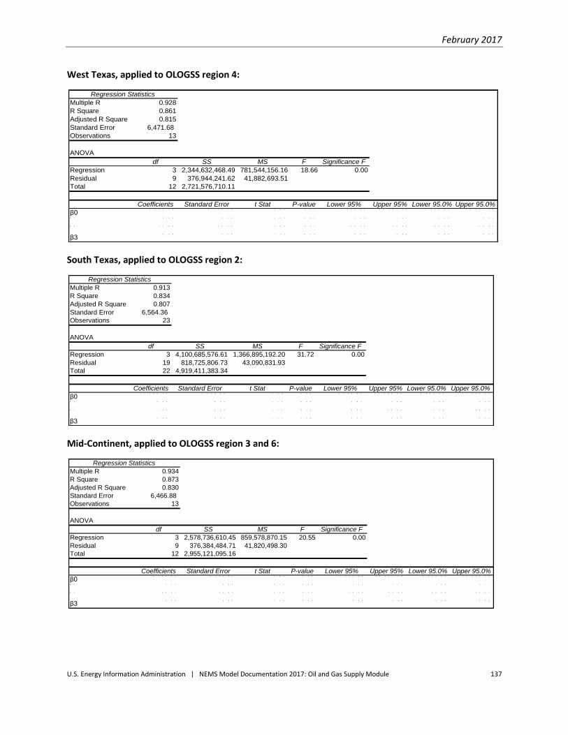
February 2017




Mid-Continent, applied to OLOGSS region 3 and 6:


Multiple R 0.928

R Square 0.861



Observations 13

ANOVA


Regression 3 2,344,632,468.49 781,544,156.16 18.66 0.00

Residual 9 376,944,241.62 41,882,693.51

Total 12 2,721,576,710.11


β04 , 4 5 0 . 2 8 5 , 2 1 9 . 4 0 0 . 8 5 0 . 4 2 - 7 , 3 5 6 . 8 4 1 6 , 2 5 7 . 4 0 - 7 , 3 5 6 . 8 4 1 6 , 2 5 7 . 4 0

β 1 2 . 5 0 0 . 4 5 5 . 5 8 0 . 0 0 1 . 4 9 3 . 5 1 1 . 4 9 3 . 5 1

β 2 2 7 . 6 5 2 1 . 2 1 1 . 3 0 0 . 2 2 - 2 0 . 3 3 7 5 . 6 3 - 2 0 . 3 3 7 5 . 6 3

β30 . 0 0 0 . 0 0 - 1 . 2 1 0 . 2 6 0 . 0 0 0 . 0 0 0 . 0 0 0 . 0 0


Multiple R 0.913

R Square 0.834



Observations 23

ANOVA


Regression 3 4,100,685,576.61 1,366,895,192.20 31.72 0.00

Residual 19 818,725,806.73 43,090,831.93

Total 22 4,919,411,383.34


β01 1 , 1 4 5 . 7 0 3 , 2 2 4 . 4 5 3 . 4 6 0 . 0 0 4 , 3 9 6 . 8 5 1 7 , 8 9 4 . 5 5 4 , 3 9 6 . 8 5 1 7 , 8 9 4 . 5 5

β 1 2 . 6 8 0 . 3 7 7 . 1 7 0 . 0 0 1 . 9 0 3 . 4 6 1 . 9 0 3 . 4 6

β 2 7 . 6 7 5 . 0 9 1 . 5 1 0 . 1 5 - 2 . 9 9 1 8 . 3 3 - 2 . 9 9 1 8 . 3 3

β30 . 0 0 0 . 0 0 - 1 . 2 1 0 . 2 4 0 . 0 0 0 . 0 0 0 . 0 0 0 . 0 0


Multiple R 0.934

R Square 0.873



Observations 13

ANOVA


Regression 3 2,578,736,610.45 859,578,870.15 20.55 0.00

Residual 9 376,384,484.71 41,820,498.30

Total 12 2,955,121,095.16


β08 , 1 9 3 . 8 2 5 , 4 1 0 . 0 4 1 . 5 1 0 . 1 6 - 4 , 0 4 4 . 5 4 2 0 , 4 3 2 . 1 8 - 4 , 0 4 4 . 5 4 2 0 , 4 3 2 . 1 8

β 1 2 . 7 5 0 . 4 5 6 . 1 4 0 . 0 0 1 . 7 4 3 . 7 7 1 . 7 4 3 . 7 7

β 2 2 1 . 2 1 1 8 . 0 4 1 . 1 8 0 . 2 7 - 1 9 . 5 9 6 2 . 0 1 - 1 9 . 5 9 6 2 . 0 1

β30 . 0 0 0 . 0 0 - 1 . 1 2 0 . 2 9 0 . 0 0 0 . 0 0 0 . 0 0 0 . 0 0

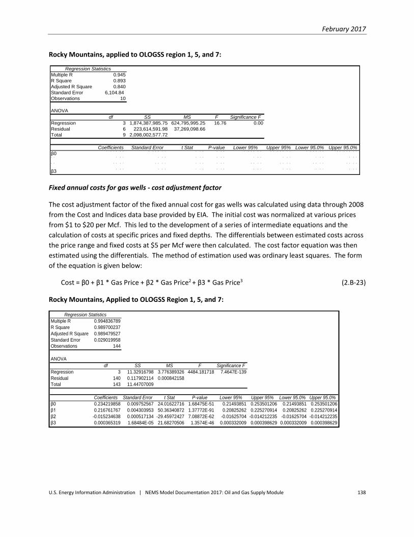
February 2017


Rocky Mountains, applied to OLOGSS region 1, 5, and 7:

Fixed annual costs for gas wells - cost adjustment factor

The cost adjustment factor of the fixed annual cost for gas wells was calculated using data through 2008

from the Cost and Indices data base provided by EIA. The initial cost was normalized at various prices

from $1 to $20 per Mcf. This led to the development of a series of intermediate equations and the


the price range and fixed costs at $5 per Mcf were then calculated. The cost factor equation was then






Multiple R 0.945

R Square 0.893



Observations 10

ANOVA


Regression 3 1,874,387,985.75 624,795,995.25 16.76 0.00

Residual 6 223,614,591.98 37,269,098.66

Total 9 2,098,002,577.72


β07 , 5 3 4 . 8 6 6 , 3 4 0 . 7 7 1 . 1 9 0 . 2 8 - 7 , 9 8 0 . 4 5 2 3 , 0 5 0 . 1 7 - 7 , 9 8 0 . 4 5 2 3 , 0 5 0 . 1 7

β 1 3 . 8 1 0 . 8 8 4 . 3 3 0 . 0 0 1 . 6 6 5 . 9 7 1 . 6 6 5 . 9 7

β 2 3 2 . 2 7 2 2 . 3 3 1 . 4 4 0 . 2 0 - 2 2 . 3 8 8 6 . 9 2 - 2 2 . 3 8 8 6 . 9 2

β30 . 0 0 0 . 0 0 - 1 . 1 8 0 . 2 8 - 0 . 0 1 0 . 0 0 - 0 . 0 1 0 . 0 0



R Square 0.989700237



Observations 144

ANOVA


Regression 3 11.32916798 3.776389326 4484.181718 7.4647E-139

Residual 140 0.117902114 0.000842158

Total 143 11.44707009


β0 0.234219858 0.009752567 24.01622716 1.68475E-51 0.21493851 0.253501206 0.21493851 0.253501206

β1 0.216761767 0.004303953 50.36340872 1.37772E-91 0.20825262 0.225270914 0.20825262 0.225270914

β2 -0.015234638 0.000517134 -29.45972427 7.08872E-62 -0.01625704 -0.014212235 -0.01625704 -0.014212235

β3 0.000365319 1.68484E-05 21.68270506 1.3574E-46 0.000332009 0.000398629 0.000332009 0.000398629

February 2017



Mid-Continent, Applied to OLOGSS Region 3 and 6:




R Square 0.991333701



Observations 144

ANOVA


Regression 3 10.42258156 3.474193854 5338.176859 4.2055E-144

Residual 140 0.091114842 0.00065082

Total 143 10.5136964


β0 0.276966489 0.008573392 32.30535588 9.09319E-67 0.260016432 0.293916546 0.260016432 0.293916546

β1 0.205740933 0.003783566 54.37751691 5.03408E-96 0.198260619 0.213221246 0.198260619 0.213221246

β2 -0.014407802 0.000454608 -31.6927929 9.63037E-66 -0.015306587 -0.013509017 -0.015306587 -0.013509017

β3 0.00034576 1.48113E-05 23.34441529 4.06714E-50 0.000316478 0.000375043 0.000316478 0.000375043



R Square 0.991199695



Observations 144

ANOVA


Regression 3 10.33109303 3.443697678 5256.179662 1.231E-143

Residual 140 0.091723972 0.000655171

Total 143 10.42281701


β0 0.278704883 0.008602002 32.40000063 6.33409E-67 0.261698262 0.295711504 0.261698262 0.295711504

β1 0.205373482 0.003796192 54.09986358 9.97995E-96 0.197868206 0.212878758 0.197868206 0.212878758

β2 -0.014404563 0.000456125 -31.58028284 1.49116E-65 -0.015306347 -0.013502779 -0.015306347 -0.013502779

β3 0.000345945 1.48607E-05 23.27919988 5.55628E-50 0.000316565 0.000375325 0.000316565 0.000375325



R Square 0.99111767



Observations 144

ANOVA


Regression 3 10.27673171 3.425577238 5207.209824 2.3566E-143

Residual 140 0.092099383 0.000657853

Total 143 10.3688311


β0 0.279731342 0.008619588 32.45298388 5.17523E-67 0.262689954 0.296772729 0.262689954 0.296772729

β1 0.205151971 0.003803953 53.93125949 1.51455E-95 0.197631352 0.21267259 0.197631352 0.21267259

β2 -0.014402579 0.000457058 -31.51151347 1.94912E-65 -0.015306207 -0.013498952 -0.015306207 -0.013498952

β3 0.00034606 1.48911E-05 23.23943141 6.72233E-50 0.00031662 0.000375501 0.00031662 0.000375501

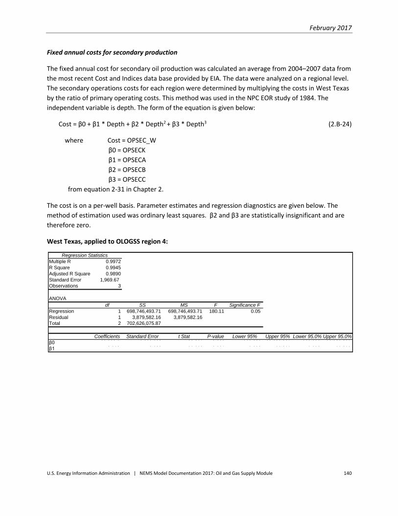
February 2017


Fixed annual costs for secondary production

The fixed annual cost for secondary oil production was calculated an average from 2004–2007 data from

the most recent Cost and Indices data base provided by EIA. The data were analyzed on a regional level.

The secondary operations costs for each region were determined by multiplying the costs in West Texas

by the ratio of primary operating costs. This method was used in the NPC EOR study of 1984. The



where Cost = OPSEC_W

β0 = OPSECK

β1 = OPSECA

β2 = OPSECB

β3 = OPSECC




therefore zero.



Multiple R 0.9972

R Square 0.9945



Observations 3

ANOVA


Regression 1 698,746,493.71 698,746,493.71 180.11 0.05

Residual 1 3,879,582.16 3,879,582.16

Total 2 702,626,075.87


β03 0 , 5 0 9 . 3 2 , 4 1 2 . 3 3 8 1 2 . 6 4 7 0 . 0 5 0 - 1 4 2 . 2 2 4 6 1 , 1 6 0 . 8 2 7 - 1 4 2 . 2 2 4 6 1 , 1 6 0 . 8 2 7

β16 . 1 1 8 0 . 4 5 6 1 3 . 4 2 0 0 . 0 4 7 0 . 3 2 6 1 1 . 9 1 1 0 . 3 2 6 1 1 . 9 1 1

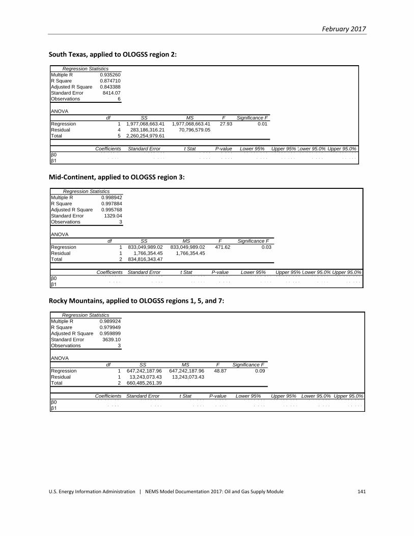
February 2017






Multiple R 0.935260

R Square 0.874710



Observations 6

ANOVA


Regression 1 1,977,068,663.41 1,977,068,663.41 27.93 0.01

Residual 4 283,186,316.21 70,796,579.05

Total 5 2,260,254,979.61


β05 5 , 7 3 2 . 7 7 , 2 8 6 . 7 9 9 7 . 6 4 8 0 . 0 0 2 3 5 , 5 0 1 . 3 1 0 7 5 , 9 6 4 . 1 8 6 3 5 , 5 0 1 . 3 1 0 7 5 , 9 6 4 . 1 8 6

β17 . 2 7 7 1 . 3 7 7 5 . 2 8 5 0 . 0 0 6 3 . 4 5 4 1 1 . 1 0 1 3 . 4 5 4 1 1 . 1 0 1


Multiple R 0.998942

R Square 0.997884



Observations 3

ANOVA


Regression 1 833,049,989.02 833,049,989.02 471.62 0.03

Residual 1 1,766,354.45 1,766,354.45

Total 2 834,816,343.47


β02 8 , 2 0 8 . 7 1 , 6 2 7 . 7 3 8 1 7 . 3 3 0 0 . 0 3 7 7 , 5 2 6 . 4 1 7 4 8 , 8 9 0 . 9 8 9 7 , 5 2 6 . 4 1 7 4 8 , 8 9 0 . 9 8 9

β16 . 6 8 0 0 . 3 0 8 2 1 . 7 1 7 0 . 0 2 9 2 . 7 7 2 1 0 . 5 8 9 2 . 7 7 2 1 0 . 5 8 9

0

50000

100000

0 20 40 60 80 100


Multiple R 0.989924

R Square 0.979949



Observations 3

ANOVA


Regression 1 647,242,187.96 647,242,187.96 48.87 0.09

Residual 1 13,243,073.43 13,243,073.43

Total 2 660,485,261.39


β05 3 , 8 5 7 . 0 6 4 , 4 5 6 . 9 7 3 1 2 . 0 8 4 0 . 0 5 3 - 2 , 7 7 3 . 9 0 9 1 1 0 , 4 8 8 . 0 3 4 - 2 , 7 7 3 . 9 0 9 1 1 0 , 4 8 8 . 0 3 4

β15 . 8 8 8 0 . 8 4 2 6 . 9 9 1 0 . 0 9 0 - 4 . 8 1 4 1 6 . 5 9 1 - 4 . 8 1 4 1 6 . 5 9 1

0

50000

100000

0 20 40 60 80 100

February 2017



Fixed annual costs for secondary production - cost adjustment factor

The cost adjustment factor of the fixed annual costs for secondary production was calculated using data










Multiple R 0.992089

R Square 0.984240



Observations 3

ANOVA


Regression 1 1,684,438,248.88 1,684,438,248.88 62.45 0.08

Residual 1 26,971,430.96 26,971,430.96

Total 2 1,711,409,679.84


β03 5 , 8 9 3 . 4 6 5 6 , 3 6 0 . 5 9 3 5 . 6 4 3 0 . 1 1 2 - 4 4 , 9 2 5 . 1 8 9 1 1 6 , 7 1 2 . 1 1 9 - 4 4 , 9 2 5 . 1 8 9 1 1 6 , 7 1 2 . 1 1 9

β19 . 4 9 9 1 . 2 0 2 7 . 9 0 3 0 . 0 8 0 - 5 . 7 7 4 2 4 . 7 7 3 - 5 . 7 7 4 2 4 . 7 7 3

0

100000

200000

0 20 40 60 80 100



R Square 0.988080495



Observations 144

ANOVA


Regression 3 8.433336986 2.811112329 3868.484883 2.0551E-134

Residual 140 0.101733815 0.00072667

Total 143 8.535070802


β0 0.325311813 0.00905922 35.90947329 1.646E-72 0.307401249 0.343222377 0.307401249 0.343222377

β1 0.019419982 0.000399797 48.57461816 1.65866E-89 0.018629562 0.020210402 0.018629562 0.020210402

β2 -0.000140009 4.80369E-06 -29.14604996 2.57525E-61 -0.000149506 -0.000130512 -0.000149506 -0.000130512

β3 3.41057E-07 1.56506E-08 21.79195958 7.87903E-47 3.10115E-07 3.71999E-07 3.10115E-07 3.71999E-07

February 2017







R Square 0.987700041



Observations 144

ANOVA


Regression 3 8.296590955 2.765530318 3747.383987 1.8532E-133

Residual 140 0.103318541 0.00073799

Total 143 8.399909496


β0 0.321750317 0.009129506 35.24290662 1.74974E-71 0.303700794 0.33979984 0.303700794 0.33979984

β1 0.019369439 0.000402899 48.0752057 6.49862E-89 0.018572887 0.020165992 0.018572887 0.020165992

β2 -0.000140208 4.84096E-06 -28.96291516 5.49447E-61 -0.000149779 -0.000130638 -0.000149779 -0.000130638

β3 3.42483E-07 1.5772E-08 21.71459435 1.15795E-46 3.11301E-07 3.73665E-07 3.11301E-07 3.73665E-07



R Square 0.988079106



Observations 144

ANOVA


Regression 3 8.43414809 2.811382697 3868.028528 2.0719E-134

Residual 140 0.101755604 0.000726826

Total 143 8.535903693


β0 0.325281756 0.00906019 35.90231108 1.68802E-72 0.307369274 0.343194238 0.307369274 0.343194238

β1 0.019420568 0.00039984 48.57088177 1.67561E-89 0.018630063 0.020211072 0.018630063 0.020211072

β2 -0.000140009 4.80421E-06 -29.14305099 2.60734E-61 -0.000149507 -0.000130511 -0.000149507 -0.000130511

β3 3.41049E-07 1.56523E-08 21.7891193 7.99109E-47 3.10103E-07 3.71994E-07 3.10103E-07 3.71994E-07



R Square 0.988082555



Observations 144

ANOVA


Regression 3 8.434398087 2.811466029 3869.161392 2.0304E-134

Residual 140 0.101728825 0.000726634

Total 143 8.536126912


β0 0.325293493 0.009058998 35.90833165 1.65262E-72 0.307383368 0.343203618 0.307383368 0.343203618

β1 0.019420405 0.000399787 48.57686713 1.64854E-89 0.018630005 0.020210806 0.018630005 0.020210806

β2 -0.000140009 4.80358E-06 -29.14672886 2.56804E-61 -0.000149505 -0.000130512 -0.000149505 -0.000130512

β3 3.41053E-07 1.56502E-08 21.792237 7.86817E-47 3.10111E-07 3.71994E-07 3.10111E-07 3.71994E-07

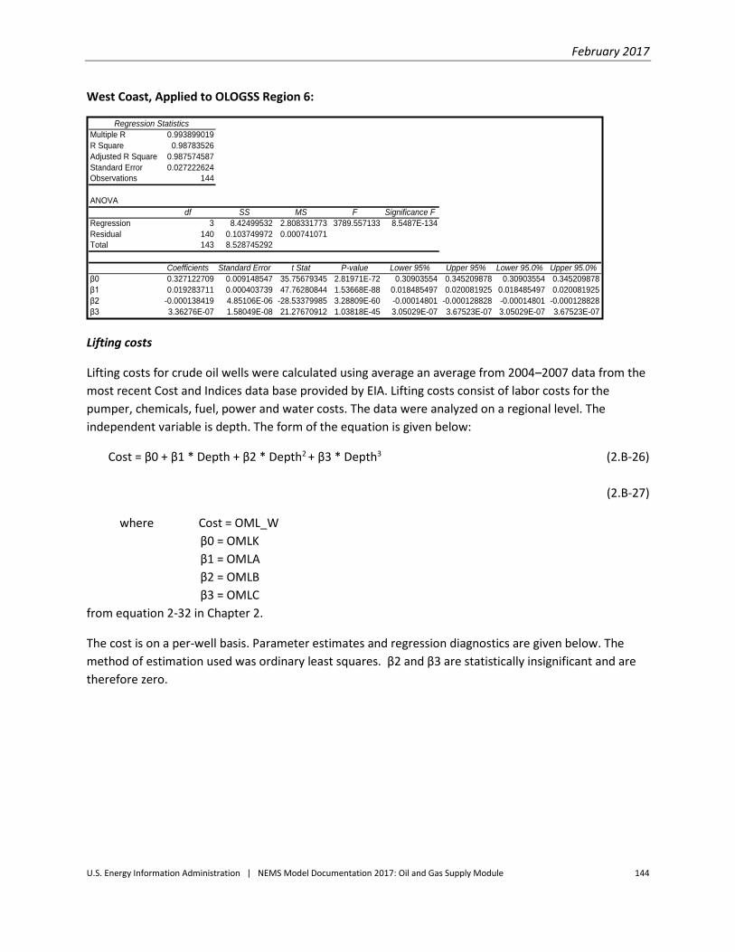
February 2017



Lifting costs

Lifting costs for crude oil wells were calculated using average an average from 2004–2007 data from the

most recent Cost and Indices data base provided by EIA. Lifting costs consist of labor costs for the

pumper, chemicals, fuel, power and water costs. The data were analyzed on a regional level. The



(2.B-27)

where Cost = OML_W

β0 = OMLK

β1 = OMLA

β2 = OMLB

β3 = OMLC




therefore zero.



R Square 0.98783526



Observations 144

ANOVA


Regression 3 8.42499532 2.808331773 3789.557133 8.5487E-134

Residual 140 0.103749972 0.000741071

Total 143 8.528745292


β0 0.327122709 0.009148547 35.75679345 2.81971E-72 0.30903554 0.345209878 0.30903554 0.345209878

β1 0.019283711 0.000403739 47.76280844 1.53668E-88 0.018485497 0.020081925 0.018485497 0.020081925

β2 -0.000138419 4.85106E-06 -28.53379985 3.28809E-60 -0.00014801 -0.000128828 -0.00014801 -0.000128828

β3 3.36276E-07 1.58049E-08 21.27670912 1.03818E-45 3.05029E-07 3.67523E-07 3.05029E-07 3.67523E-07

February 2017






Multiple R 0.9994

R Square 0.9988



Observations 3

ANOVA


Regression 1 15,852,301 15,852,301 849 0

Residual 1 18,681 18,681

Total 2 15,870,982


β07 , 5 3 4 . 5 1 5 1 6 7 . 3 9 5 4 5 . 0 1 0 0 . 0 1 4 5 , 4 0 7 . 5 6 5 9 , 6 6 1 . 4 6 5 5 , 4 0 7 . 5 6 5 9 , 6 6 1 . 4 6 5

β10 . 9 2 2 0 . 0 3 2 2 9 . 1 3 1 0 . 0 2 2 0 . 5 2 0 1 . 3 2 3 0 . 5 2 0 1 . 3 2 3


Multiple R 0.8546

R Square 0.7304



Observations 7

ANOVA


Regression 1 69,387,339 69,387,339 14 0

Residual 5 25,617,128 5,123,426

Total 6 95,004,467


β01 1 , 5 8 5 . 1 9 1 1 , 6 5 4 . 4 4 0 7 . 0 0 2 0 . 0 0 1 7 , 3 3 2 . 3 2 4 1 5 , 8 3 8 . 0 5 8 7 , 3 3 2 . 3 2 4 1 5 , 8 3 8 . 0 5 8

β10 . 9 1 2 0 . 2 4 8 3 . 6 8 0 0 . 0 1 4 0 . 2 7 5 1 . 5 4 9 0 . 2 7 5 1 . 5 4 9


Multiple R 0.9997

R Square 0.9995


Standard Error 82.0

Observations 3

ANOVA


Regression 1 13,261,874 13,261,874 1,972 0

Residual 1 6,726 6,726

Total 2 13,268,601


β08 , 2 9 8 . 3 3 9 1 0 0 . 4 4 7 8 2 . 6 1 4 0 . 0 0 8 7 , 0 2 2 . 0 4 5 9 , 5 7 4 . 6 3 4 7 , 0 2 2 . 0 4 5 9 , 5 7 4 . 6 3 4

β10 . 8 4 3 0 . 0 1 9 4 4 . 4 0 3 0 . 0 1 4 0 . 6 0 2 1 . 0 8 4 0 . 6 0 2 1 . 0 8 4

February 2017




Lifting costs - cost adjustment factor

The cost adjustment factor for lifting costs was calculated using data through 2008 from the Cost and

Indices data base provided by EIA. The initial cost was normalized at various prices from $10 to $200

per barrel. This led to the development of a series of intermediate equations and the calculation of

costs at specific prices and fixed depths. The differentials between estimated costs across the price

range and fixed costs at $50 per barrel were then calculated. The cost factor equation was then





Multiple R 1.0000

R Square 1.0000


Standard Error 11.5

Observations 3

ANOVA


Regression 1 3,979,238 3,979,238 30,138 0

Residual 1 132 132

Total 2 3,979,370


β01 0 , 1 3 7 . 3 9 8 1 4 . 0 7 3 7 2 0 . 3 4 2 0 . 0 0 1 9 , 9 5 8 . 5 8 4 1 0 , 3 1 6 . 2 1 2 9 , 9 5 8 . 5 8 4 1 0 , 3 1 6 . 2 1 2

β10 . 4 6 2 0 . 0 0 3 1 7 3 . 6 0 3 0 . 0 0 4 0 . 4 2 8 0 . 4 9 5 0 . 4 2 8 0 . 4 9 5


Multiple R 0.9969

R Square 0.9937



Observations 3

ANOVA


Regression 1 203,349,853 203,349,853 158 0

Residual 1 1,286,583 1,286,583

Total 2 204,636,436


β05 , 1 4 7 . 3 1 3 1 , 3 8 9 . 1 9 9 3 . 7 0 5 0 . 1 6 8 - 1 2 , 5 0 4 . 0 6 3 2 2 , 7 9 8 . 6 8 9 - 1 2 , 5 0 4 . 0 6 3 2 2 , 7 9 8 . 6 8 9

β13 . 3 0 1 0 . 2 6 3 1 2 . 5 7 2 0 . 0 5 1 - 0 . 0 3 5 6 . 6 3 6 - 0 . 0 3 5 6 . 6 3 6

February 2017







R Square 0.988869972



Observations 144

ANOVA


Regression 3 8.900010642 2.966670214 4146.195026 1.6969E-136

Residual 140 0.100172285 0.000715516

Total 143 9.000182927


β0 0.314447949 0.008989425 34.97976138 4.49274E-71 0.296675373 0.332220525 0.296675373 0.332220525

β1 0.019667961 0.000396717 49.57683267 1.11119E-90 0.018883631 0.020452291 0.018883631 0.020452291

β2 -0.000140635 4.76668E-06 -29.50377541 5.91881E-62 -0.000150059 -0.000131211 -0.000150059 -0.000131211

β3 3.41221E-07 1.553E-08 21.97170644 3.23018E-47 3.10517E-07 3.71924E-07 3.10517E-07 3.71924E-07



R Square 0.989479094



Observations 144

ANOVA


Regression 3 9.177423888 3.059141296 4388.946164 3.302E-138

Residual 140 0.097581462 0.00069701

Total 143 9.275005349


β0 0.307250046 0.008872414 34.62981435 1.58839E-70 0.289708807 0.324791284 0.289708807 0.324791284

β1 0.019843369 0.000391553 50.6786443 6.01683E-92 0.019069248 0.020617491 0.019069248 0.020617491

β2 -0.000141338 4.70464E-06 -30.04217841 6.6318E-63 -0.000150639 -0.000132036 -0.000150639 -0.000132036

β3 3.42235E-07 1.53279E-08 22.32765206 5.59173E-48 3.11931E-07 3.72539E-07 3.11931E-07 3.72539E-07



R Square 0.989280214



Observations 144

ANOVA


Regression 3 9.087590035 3.029196678 4306.653909 1.2247E-137

Residual 140 0.09847263 0.000703376

Total 143 9.186062664


β0 0.309274775 0.008912836 34.69993005 1.23231E-70 0.291653621 0.32689593 0.291653621 0.32689593

β1 0.019797213 0.000393337 50.33145871 1.49879E-91 0.019019565 0.020574861 0.019019565 0.020574861

β2 -0.000141221 4.72607E-06 -29.88132995 1.27149E-62 -0.000150565 -0.000131878 -0.000150565 -0.000131878

β3 3.42202E-07 1.53977E-08 22.22423366 9.29272E-48 3.1176E-07 3.72644E-07 3.1176E-07 3.72644E-07

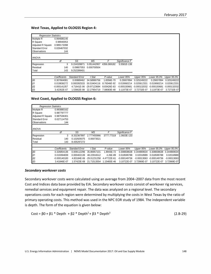
February 2017




Secondary workover costs

Secondary workover costs were calculated using an average from 2004–2007 data from the most recent

Cost and Indices data base provided by EIA. Secondary workover costs consist of workover rig services,

remedial services and equipment repair. The data was analyzed on a regional level. The secondary

operations costs for each region were determined by multiplying the costs in West Texas by the ratio of

primary operating costs. This method was used in the NPC EOR study of 1984. The independent variable

is depth. The form of the equation is given below:




R Square 0.98940053



Observations 144

ANOVA


Regression 3 9.154328871 3.051442957 4356.069182 5.5581E-138

Residual 140 0.09807053 0.000700504

Total 143 9.252399401


β0 0.307664081 0.00889462 34.58990756 1.8356E-70 0.29007894 0.325249222 0.29007894 0.325249222

β1 0.019836272 0.000392533 50.53404116 8.79346E-92 0.019060214 0.020612331 0.019060214 0.020612331

β2 -0.000141357 4.71641E-06 -29.97123684 8.83426E-63 -0.000150681 -0.000132032 -0.000150681 -0.000132032

β3 3.42352E-07 1.53662E-08 22.27954719 7.08083E-48 3.11973E-07 3.72732E-07 3.11973E-07 3.72732E-07



R Square 0.987797777



Observations 144

ANOVA


Regression 3 8.332367897 2.777455966 3777.77319 1.0603E-133

Residual 140 0.102929375 0.00073521

Total 143 8.435297272


β0 0.326854136 0.009112296 35.86957101 1.8943E-72 0.308838638 0.344869634 0.308838638 0.344869634

β1 0.019394839 0.000402139 48.22916512 4.26E-89 0.018599788 0.02018989 0.018599788 0.02018989

β2 -0.000140183 4.83184E-06 -29.01231258 4.47722E-61 -0.000149736 -0.00013063 -0.000149736 -0.00013063

β3 3.41846E-07 1.57423E-08 21.71513554 1.15483E-46 3.10722E-07 3.72969E-07 3.10722E-07 3.72969E-07

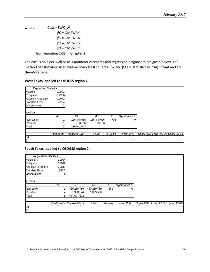
February 2017


where Cost = SWK_W

β0 = OMSWRK

β1 = OMSWRA

β2 = OMSWRB

β3 = OMSWRC




therefore zero.




Multiple R 0.9993

R Square 0.9986



Observations 3

ANOVA


Regression 1 136,348,936 136,348,936 706 0

Residual 1 193,106 193,106

Total 2 136,542,042


β04 , 9 5 1 . 0 5 9 5 3 8 . 2 0 0 9 . 1 9 9 0 . 0 6 9 - 1 , 8 8 7 . 3 9 2 1 1 , 7 8 9 . 5 1 0 - 1 , 8 8 7 . 3 9 2 1 1 , 7 8 9 . 5 1 0

β12 . 7 0 3 0 . 1 0 2 2 6 . 5 7 2 0 . 0 2 4 1 . 4 1 0 3 . 9 9 5 1 . 4 1 0 3 . 9 9 5


Multiple R 0.9924

R Square 0.9849



Observations 6

ANOVA


Regression 1 480,269,759 480,269,759 261 0

Residual 4 7,358,144 1,839,536

Total 5 487,627,903


β01 0 , 5 6 0 . 0 6 9 1 , 1 7 4 . 5 8 6 8 . 9 9 0 0 . 0 0 1 7 , 2 9 8 . 8 8 9 1 3 , 8 2 1 . 2 4 9 7 , 2 9 8 . 8 8 9 1 3 , 8 2 1 . 2 4 9

β13 . 5 8 7 0 . 2 2 2 1 6 . 1 5 8 0 . 0 0 0 2 . 9 7 0 4 . 2 0 3 2 . 9 7 0 4 . 2 0 3

February 2017






Multiple R 0.9989

R Square 0.9979



Observations 3

ANOVA


Regression 1 140,143,261 140,143,261 473 0

Residual 1 296,583 296,583

Total 2 140,439,844


β03 , 7 3 2 . 5 1 0 6 6 6 . 9 8 9 5 . 5 9 6 0 . 1 1 3 - 4 , 7 4 2 . 3 5 5 1 2 , 2 0 7 . 3 7 5 - 4 , 7 4 2 . 3 5 5 1 2 , 2 0 7 . 3 7 5

β12 . 7 4 0 0 . 1 2 6 2 1 . 7 3 8 0 . 0 2 9 1 . 1 3 8 4 . 3 4 2 1 . 1 3 8 4 . 3 4 2


Multiple R 0.9996

R Square 0.9991



Observations 3

ANOVA


Regression 1 98,740,186 98,740,186 1,167 0

Residual 1 84,627 84,627

Total 2 98,824,812


β05 , 2 9 1 . 9 5 4 3 5 6 . 2 8 7 1 4 . 8 5 3 0 . 0 4 3 7 6 4 . 9 2 2 9 , 8 1 8 . 9 8 7 7 6 4 . 9 2 2 9 , 8 1 8 . 9 8 7

β12 . 3 0 0 0 . 0 6 7 3 4 . 1 5 8 0 . 0 1 9 1 . 4 4 4 3 . 1 5 5 1 . 4 4 4 3 . 1 5 5


Multiple R 0.9991

R Square 0.9983



Observations 3

ANOVA


Regression 1 120,919,119 120,919,119 585 0

Residual 1 206,762 206,762

Total 2 121,125,881


β04 , 1 3 1 . 4 8 6 5 5 6 . 9 0 5 7 . 4 1 9 0 . 0 8 5 - 2 , 9 4 4 . 6 3 8 1 1 , 2 0 7 . 6 1 0 - 2 , 9 4 4 . 6 3 8 1 1 , 2 0 7 . 6 1 0

β12 . 5 4 5 0 . 1 0 5 2 4 . 1 8 3 0 . 0 2 6 1 . 2 0 8 3 . 8 8 2 1 . 2 0 8 3 . 8 8 2

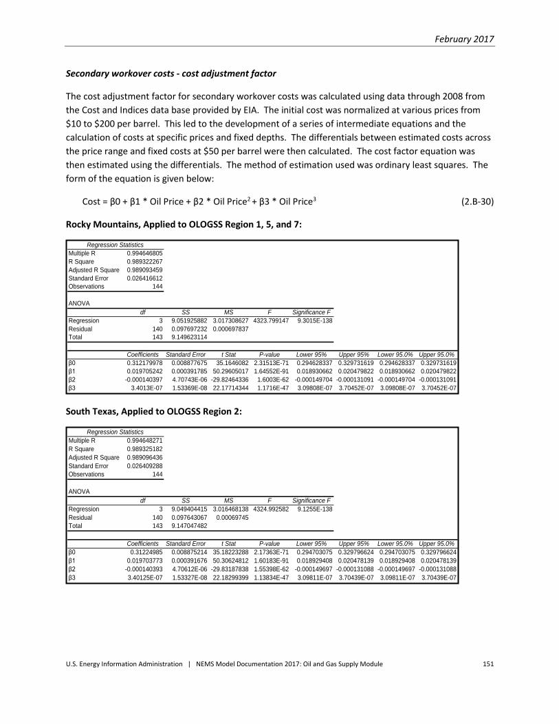
February 2017


Secondary workover costs - cost adjustment factor

The cost adjustment factor for secondary workover costs was calculated using data through 2008 from

the Cost and Indices data base provided by EIA. The initial cost was normalized at various prices from

$10 to $200 per barrel. This led to the development of a series of intermediate equations and the


the price range and fixed costs at $50 per barrel were then calculated. The cost factor equation was

then estimated using the differentials. The method of estimation used was ordinary least squares. The

form of the equation is given below:






R Square 0.989322267



Observations 144

ANOVA


Regression 3 9.051925882 3.017308627 4323.799147 9.3015E-138

Residual 140 0.097697232 0.000697837

Total 143 9.149623114


β0 0.312179978 0.008877675 35.1646082 2.31513E-71 0.294628337 0.329731619 0.294628337 0.329731619

β1 0.019705242 0.000391785 50.29605017 1.64552E-91 0.018930662 0.020479822 0.018930662 0.020479822

β2 -0.000140397 4.70743E-06 -29.82464336 1.6003E-62 -0.000149704 -0.000131091 -0.000149704 -0.000131091

β3 3.4013E-07 1.53369E-08 22.17714344 1.1716E-47 3.09808E-07 3.70452E-07 3.09808E-07 3.70452E-07



R Square 0.989325182



Observations 144

ANOVA


Regression 3 9.049404415 3.016468138 4324.992582 9.1255E-138

Residual 140 0.097643067 0.00069745

Total 143 9.147047482


β0 0.31224985 0.008875214 35.18223288 2.17363E-71 0.294703075 0.329796624 0.294703075 0.329796624

β1 0.019703773 0.000391676 50.30624812 1.60183E-91 0.018929408 0.020478139 0.018929408 0.020478139

β2 -0.000140393 4.70612E-06 -29.83187838 1.55398E-62 -0.000149697 -0.000131088 -0.000149697 -0.000131088

β3 3.40125E-07 1.53327E-08 22.18299399 1.13834E-47 3.09811E-07 3.70439E-07 3.09811E-07 3.70439E-07

February 2017







R Square 0.988815263



Observations 144

ANOVA


Regression 3 9.269694355 3.089898118 4125.685804 2.3918E-136

Residual 140 0.104851837 0.000748942

Total 143 9.374546192


β0 0.301399555 0.009196999 32.7715099 1.54408E-67 0.283216594 0.319582517 0.283216594 0.319582517

β1 0.020285999 0.000405877 49.980617 3.79125E-91 0.019483558 0.021088441 0.019483558 0.021088441

β2 -0.000145269 4.87675E-06 -29.78803686 1.85687E-62 -0.00015491 -0.000135627 -0.00015491 -0.000135627

β3 3.51144E-07 1.58886E-08 22.10035946 1.71054E-47 3.19731E-07 3.82556E-07 3.19731E-07 3.82556E-07



R Square 0.989320233



Observations 144

ANOVA


Regression 3 9.054508298 3.018169433 4322.966602 9.4264E-138

Residual 140 0.097743924 0.000698171

Total 143 9.152252223


β0 0.312146343 0.008879797 35.15242029 2.41837E-71 0.294590508 0.329702178 0.294590508 0.329702178

β1 0.019706241 0.000391879 50.28658391 1.68714E-91 0.018931476 0.020481006 0.018931476 0.020481006

β2 -0.000140397 4.70855E-06 -29.81743751 1.64782E-62 -0.000149706 -0.000131088 -0.000149706 -0.000131088

β3 3.4012E-07 1.53406E-08 22.17121727 1.20629E-47 3.09791E-07 3.70449E-07 3.09791E-07 3.70449E-07



R Square 0.989316964



Observations 144

ANOVA


Regression 3 9.05566979 3.018556597 4321.629647 9.6305E-138

Residual 140 0.097786705 0.000698476

Total 143 9.153456495


β0 0.312123671 0.00888174 35.14217734 2.50872E-71 0.294563994 0.329683347 0.294563994 0.329683347

β1 0.019707015 0.000391964 50.27755672 1.72782E-91 0.01893208 0.020481949 0.01893208 0.020481949

β2 -0.0001404 4.70958E-06 -29.81159891 1.68736E-62 -0.000149711 -0.000131089 -0.000149711 -0.000131089

β3 3.40124E-07 1.5344E-08 22.16666321 1.23366E-47 3.09789E-07 3.7046E-07 3.09789E-07 3.7046E-07

February 2017


Additional cost equations and factors

The model uses several updated cost equations and factors originally developed for DOE/NETL’s

Comprehensive Oil and Gas Analysis Model (COGAM). These are:

The crude oil and natural gas investment factors for tangible and intangible investments as well

as the operating costs. These factors were originally developed based upon the 1984 Enhanced

Oil Recovery Study completed by NPC.

The G&A factors for capitalized and expensed costs.

The limits on impurities, such as N2, CO2, and H2S used to calculate natural gas processing costs.

Cost equations for stimulation, the produced water handling plant, the chemical handling plant,

the polymer handling plant, CO2 recycling plant, and the steam manifolds and pipelines.

Natural and industrial CO2 prices

The model uses regional CO2 prices for both natural and industrial sources of CO2. The cost equation for

natural CO2 is derived from the equation used in COGAM and updated to reflect current dollar values.

According to University of Wyoming, this equation is applicable to the natural CO2 in the Permian basin

(Southwest). The cost of CO2 in other regions and states is calculated using state calibration factors

which represent the additional cost of transportation.

The industrial CO2 costs contain two components: cost of capture and cost of transportation. The

capture costs are derived using data obtained from Denbury Resources, Inc. and other sources. CO2

capture costs range between $20 and $63/ton. The transportation costs were derived using an external

economic model which calculates pipeline tariff based upon average distance, compression rate, and

volume of CO2 transported.

National and regional drilling footage

National footage equations are used to determine the total drilling footage available for oil, gas, and dry

wells in two categories: development and exploration. The calculated footage is then allocated to the

OLOGSS region using well-category specific regional distributions. In this section both the national

equation and the regional distribution will be provided for each of the six drilling categories.

Oil development footage

The equation for oil drilling footage was estimated for the time period 2000–2009. The drilling footage

data were compiled from EIA’s Annual Energy Review 2010 and the 2011 Monthly Energy Review. The

form of the estimating equation is given by:

Oil Footage = β0 + β1 * Oil Price + β2 * Oil Price3 + β3 * Oil Price * Gas Price (2.B-31)

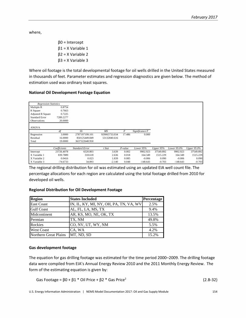
February 2017


where,

β0 = Intercept

β1 = X Variable 1

β2 = X Variable 2

β3 = X Variable 3

Where oil footage is the total developmental footage for oil wells drilled in the United States measured

in thousands of feet. Parameter estimates and regression diagnostics are given below. The method of

estimation used was ordinary least squares.

National Oil Development Footage Equation

The regional drilling distribution for oil was estimated using an updated EIA well count file. The

percentage allocations for each region are calculated using the total footage drilled from 2010 for

developed oil wells.

Regional Distribution for Oil Development Footage

Gas development footage

The equation for gas drilling footage was estimated for the time period 2000–2009. The drilling footage



Gas Footage = β0 + β1 * Oil Price + β2 * Gas Price2 (2.B-32)


Multiple R 0.8754

R Square 0.7663



Observations 20.0000

ANOVA


Regression 3.0000 2787197199.101 929065733.034 17.486 0.000

Residual 16.0000 850125449.849 53132840.616

Total 19.0000 3637322648.950


Intercept 23726.4078 6520.803 3.639 0.002 9902.923 37549.892 9902.923 37549.892

X Variable 1 839.7889 318.618 2.636 0.018 164.349 1515.229 164.349 1515.229

X Variable 2 0.0416 0.023 1.839 0.085 -0.006 0.090 -0.006 0.090

X Variable 3 -74.6733 34.893 -2.140 0.048 -148.643 -0.703 -148.643 -0.703

Region States Included Percentage

East Coast IN, IL, KY, MI, NY, OH, PA, TN, VA, WV 2.5%

Gulf Coast AL, FL, LA, MS, TX 9.4%

Midcontinent AR, KS, MO, NE, OK, TX 13.5%

Permian TX, NM 49.8%

Rockies CO, NV, UT, WY, NM 5.5%

West Coast CA, WA 4.2%

Northern Great Plains MT, ND, SD 15.2%

February 2017


where,

β0 = Intercept

β1 = X Variable 1

β2 = X Variable 2

Where gas footage is the total developmental footage for gas wells drilled in the United States

measured in thousands of feet. Parameter estimates and regression diagnostics are given below. The

method of estimation used was ordinary least squares.

National Gas Development Footage Equation

The regional drilling distribution for gas was estimated using an updated EIA well count file. The

percentage allocations for each region are calculated using the total footage drilled from 2010 for

developed gas wells.

Regional Distribution for Gas Development Footage

Dry development footage

The equation for dry drilling footage was estimated for the time period 2000−2009. The drilling footage



Dry Footage = β0 + β1 Oil Price2 + β2 * Oil Price3 + β3 * Gas Price + β4 + Gas Price2 (2.B-33)


Multiple R 0.9600

R Square 0.9216




ANOVA


Regression 2.0000 52118056316.202 26059028158.101 99.951 0.000

Residual 17.0000 4432227190.598 260719246.506

Total 19.0000 56550283506.800


Intercept 14602.8232 7781.097 1.877 0.078 -1813.856 31019.502 -1813.856 31019.502

X Variable 1 1513.3128 322.721 4.689 0.000 832.431 2194.195 832.431 2194.195

X Variable 2 1131.8266 340.064 3.328 0.004 414.355 1849.298 414.355 1849.298





Permian TX, NM 7.9%




February 2017


where,

β0 = Intercept

β1 = X Variable 1

β2 = X Variable 2

β3 = X Variable 3

β4 = X Variable 4

Where dry footage is the total developmental footage for dry wells drilled in the United States

measured in thousands of feet. Parameter estimates and regression diagnostics are given below. The

method of estimation used was ordinary least squares.

National Dry Development Footage Equation

The regional drilling distributions for developmental dry footage was estimated using an updated EIA

well count file. The percentage allocations for each region are calculated using the total footage drilled

from 2010 for developed dry wells.

Regional Distribution for Dry Development Footage

SUMMARY OUTPUT


Multiple R 0.3724

R Square 0.1387

Adjusted R Square -0.0910



ANOVA


Regression 4.0000 19629082.563 4907270.641 0.604 0.666

Residual 15.0000 121874991.987 8124999.466

Total 19.0000 141504074.550


Intercept 22111.8088 5591.033 3.955 0.001 10194.804 34028.814 10194.804 34028.814

X Variable 1 0.3689 2.153 0.171 0.866 -4.219 4.957 -4.219 4.957

X Variable 2 0.0002 0.021 0.011 0.991 -0.045 0.046 -0.045 0.046

X Variable 3 -2768.8619 2682.080 -1.032 0.318 -8485.580 2947.856 -8485.580 2947.856

X Variable 4 241.4373 264.236 0.914 0.375 -321.769 804.643 -321.769 804.643









February 2017


Oil exploration footage

The equation for oil drilling footage was estimated for the time period 2000–2009. The drilling footage



Oil Footage = β0 + β1 Oil Price2 + β2 * Gas Price + β3 * Gas Price * Oil Price2 (2.B-34)

where,

β0 = Intercept

β1 = X Variable 1

β2 = X Variable 2

β3 = X Variable 3

Where oil footage is the total footage of oil exploration wells drilled in the United States measured in

thousands of feet. Parameter estimates and regression diagnostics are given below. The method of


National Oil Exploration Footage Equation

The regional drilling distribution for oil exploration was estimated using an updated EIA well count file.

The percentage allocations for each region are calculated using the total footage drilled from 2010 for

oil exploration wells.


Multiple R 0.8554

R Square 0.7317




ANOVA


Regression 3.0000 34111589.936 11370529.979 14.543 0.000

Residual 16.0000 12509993.264 781874.579

Total 19.0000 46621583.200


Intercept 3700.2033 701.868 5.272 0.000 2212.310 5188.097 2212.310 5188.097

X Variable 1 1.6432 0.542 3.032 0.008 0.494 2.792 0.494 2.792

X Variable 2 -356.1698 173.459 -2.053 0.057 -723.886 11.547 -723.886 11.547

X Variable 3 -0.1084 0.071 -1.531 0.145 -0.258 0.042 -0.258 0.042

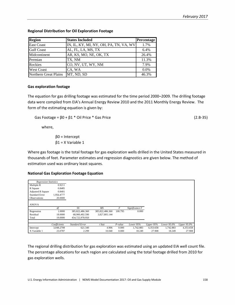
February 2017


Regional Distribution for Oil Exploration Footage

Gas exploration footage

The equation for gas drilling footage was estimated for the time period 2000–2009. The drilling footage



Gas Footage = β0 + β1 * Oil Price * Gas Price (2.B-35)

where,

β0 = Intercept

β1 = X Variable 1

Where gas footage is the total footage for gas exploration wells drilled in the United States measured in



National Gas Exploration Footage Equation

The regional drilling distribution for gas exploration was estimated using an updated EIA well count file.


gas exploration wells.










Multiple R 0.9211

R Square 0.8485




ANOVA


Regression 1.0000 385,822,486.360 385,822,486.360 100.795 0.000

Residual 18.0000 68,900,492.590 3,827,805.144

Total 19.0000 454,722,978.950


Intercept 3,048.2708 621.340 4.906 0.000 1,742.883 4,353.658 1,742.883 4,353.658

X Variable 1 23.0787 2.299 10.040 0.000 18.249 27.908 18.249 27.908

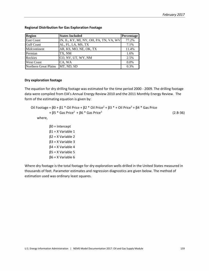
February 2017


Regional Distribution for Gas Exploration Footage

Dry exploration footage

The equation for dry drilling footage was estimated for the time period 2000 - 2009. The drilling footage



Oil Footage = β0 + β1 * Oil Price + β2 * Oil Price2 + β3 * + Oil Price3 + β4 * Gas Price

+ β5 * Gas Price2 + β6 * Gas Price3 (2.B-36)

where,

β0 = Intercept

β1 = X Variable 1

β2 = X Variable 2

β3 = X Variable 3

β4 = X Variable 4

β5 = X Variable 5

β6 = X Variable 6

Where dry footage is the total footage for dry exploration wells drilled in the United States measured in







Permian TX, NM 1.6%




February 2017


National Dry Exploration Footage Equation

The regional drilling distribution for dry exploration was estimated using an updated EIA well count file.


dry exploration wells.

Regional Distribution for Dry Exploration Footage

Regional rig depth rating

The regional rig depth ratings were determined using historical rig count data between 2005 and 2010

from Smith Bits. The depth rating was calculated for each rig, the rig was classified as either oil or gas,

and it was assigned to a particular OLOGSS region.

The percentages are applied to the regional drilling footage available in order to determine the footage

which can be drilled in each of the depth categories.


Multiple R 0.6519

R Square 0.4249




ANOVA


Regression 6.0000 92905332.768 15484222.128 1.601 0.224

Residual 13.0000 125741227.232 9672402.095

Total 19.0000 218646560.000


Intercept 28226.7366 18990.122 1.486 0.161 -12798.927 69252.400 -12798.927 69252.400

X Variable 1 1213.0103 641.922 1.890 0.081 -173.779 2599.799 -173.779 2599.799

X Variable 2 -23.4564 12.533 -1.872 0.084 -50.533 3.620 -50.533 3.620

X Variable 3 0.1356 0.074 1.832 0.090 -0.024 0.296 -0.024 0.296

X Variable 4 -19000.6302 13470.813 -1.411 0.182 -48102.551 10101.291 -48102.551 10101.291

X Variable 5 3125.5097 2686.975 1.163 0.266 -2679.346 8930.366 -2679.346 8930.366

X Variable 6 -165.2930 168.229 -0.983 0.344 -528.730 198.144 -528.730 198.144





Permian TX, NM 8.6%




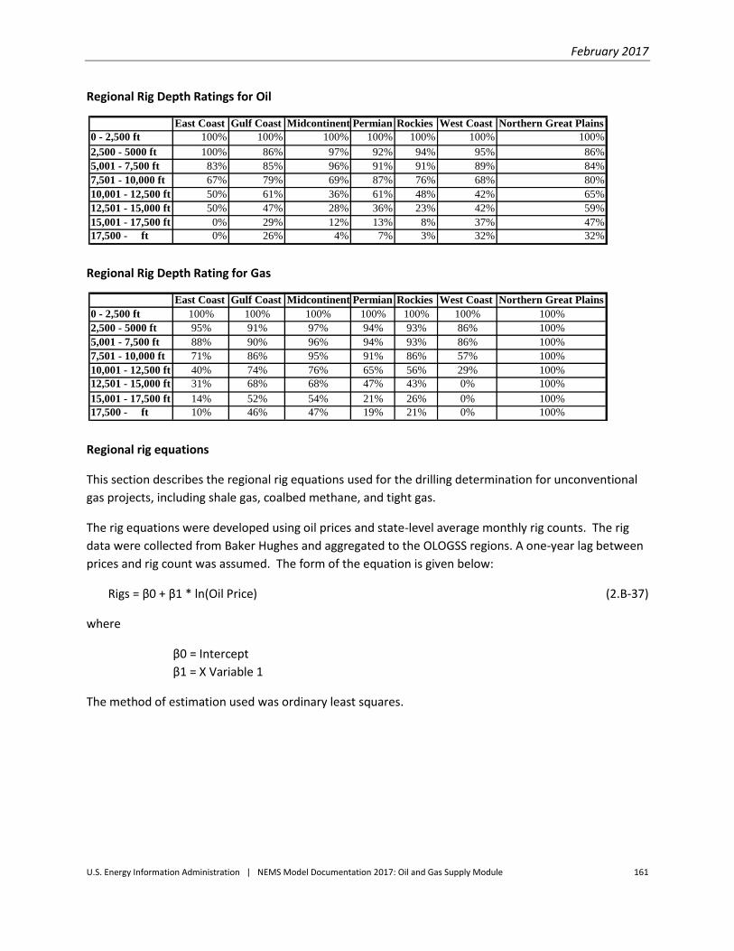
February 2017


Regional Rig Depth Ratings for Oil

Regional Rig Depth Rating for Gas

Regional rig equations

This section describes the regional rig equations used for the drilling determination for unconventional

gas projects, including shale gas, coalbed methane, and tight gas.

The rig equations were developed using oil prices and state-level average monthly rig counts. The rig

data were collected from Baker Hughes and aggregated to the OLOGSS regions. A one-year lag between

prices and rig count was assumed. The form of the equation is given below:

Rigs = β0 + β1 * ln(Oil Price) (2.B-37)

where

β0 = Intercept

β1 = X Variable 1

The method of estimation used was ordinary least squares.

East Coast Gulf Coast Midcontinent Permian Rockies West Coast Northern Great Plains

0 - 2,500 ft 100% 100% 100% 100% 100% 100% 100%

2,500 - 5000 ft 100% 86% 97% 92% 94% 95% 86%

5,001 - 7,500 ft 83% 85% 96% 91% 91% 89% 84%

7,501 - 10,000 ft 67% 79% 69% 87% 76% 68% 80%

10,001 - 12,500 ft 50% 61% 36% 61% 48% 42% 65%

12,501 - 15,000 ft 50% 47% 28% 36% 23% 42% 59%

15,001 - 17,500 ft 0% 29% 12% 13% 8% 37% 47%

17,500 - ft 0% 26% 4% 7% 3% 32% 32%

East Coast Gulf Coast Midcontinent Permian Rockies West Coast Northern Great Plains

0 - 2,500 ft 100% 100% 100% 100% 100% 100% 100%

2,500 - 5000 ft 95% 91% 97% 94% 93% 86% 100%

5,001 - 7,500 ft 88% 90% 96% 94% 93% 86% 100%

7,501 - 10,000 ft 71% 86% 95% 91% 86% 57% 100%

10,001 - 12,500 ft 40% 74% 76% 65% 56% 29% 100%

12,501 - 15,000 ft 31% 68% 68% 47% 43% 0% 100%

15,001 - 17,500 ft 14% 52% 54% 21% 26% 0% 100%

17,500 - ft 10% 46% 47% 19% 21% 0% 100%

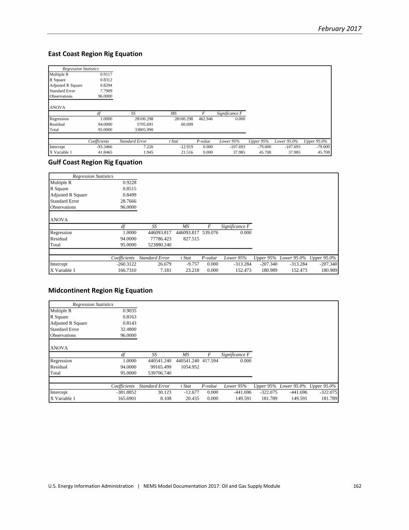
February 2017


East Coast Region Rig Equation

Gulf Coast Region Rig Equation

Midcontinent Region Rig Equation


Multiple R 0.9228

R Square 0.8515




ANOVA


Regression 1.0000 446093.817 446093.817 539.076 0.000

Residual 94.0000 77786.423 827.515

Total 95.0000 523880.240


Intercept -260.3122 26.679 -9.757 0.000 -313.284 -207.340 -313.284 -207.340

X Variable 1 166.7310 7.181 23.218 0.000 152.473 180.989 152.473 180.989


Multiple R 0.9035

R Square 0.8163




ANOVA


Regression 1.0000 440541.240 440541.240 417.594 0.000

Residual 94.0000 99165.499 1054.952

Total 95.0000 539706.740


Intercept -381.8852 30.123 -12.677 0.000 -441.696 -322.075 -441.696 -322.075

X Variable 1 165.6901 8.108 20.435 0.000 149.591 181.789 149.591 181.789


Multiple R 0.9117

R Square 0.8312




ANOVA


Regression 1.0000 28100.298 28100.298 462.946 0.000

Residual 94.0000 5705.691 60.699

Total 95.0000 33805.990


Intercept -93.3466 7.226 -12.919 0.000 -107.693 -79.000 -107.693 -79.000

X Variable 1 41.8465 1.945 21.516 0.000 37.985 45.708 37.985 45.708

February 2017


Southwest Region Rig Equation

Rocky Mountain Region Rig Equation

West Coast Region Rig Equation


Multiple R 0.9495

R Square 0.9015




ANOVA


Regression 1.0000 1366991.026 1366991.026 860.744 0.000

Residual 94.0000 149286.075 1588.150

Total 95.0000 1516277.102


Intercept -761.8706 36.960 -20.613 0.000 -835.255 -688.486 -835.255 -688.486

X Variable 1 291.8677 9.948 29.338 0.000 272.115 311.620 272.115 311.620


Multiple R 0.9185

R Square 0.8436




ANOVA


Regression 1.0000 344290.807 344290.807 507.095 0.000

Residual 94.0000 63821.003 678.947

Total 95.0000 408111.810


Intercept -340.2829 24.166 -14.081 0.000 -388.265 -292.301 -388.265 -292.301

X Variable 1 146.4758 6.505 22.519 0.000 133.561 159.391 133.561 159.391


Multiple R 0.8970

R Square 0.8046




ANOVA


Regression 1.0000 4558.709 4558.709 288.247 0.000

Residual 70.0000 1107.069 15.815

Total 71.0000 5665.778


Intercept -48.6162 4.540 -10.708 0.000 -57.671 -39.561 -57.671 -39.561

X Variable 1 20.1000 1.184 16.978 0.000 17.739 22.461 17.739 22.461

February 2017


Northern Great Plains Region Rig Equation

Regional dry hole rates

The OLOGSS model uses three dry hole rates in the economic and footage calculations. These rates are

for: 1) existing and discovered projects, 2) the first well drilled in an exploration oil or gas project, and 3)

the subsequent wells drilled in that project. In this section, the development and values for each of

these three rates will be described.

Discovered projects

The percentage allocation for existing regional dry hole rates was estimated using an updated EIA well

count file. The percentage is determined by the average footage drilled from 2010 for each

corresponding region. Existing dry hole rates calculate the projects which have already been discovered.

The formula for the percentage is given below:

Existing Dry Hole Rate = Developed Dry Hole / Total Drilling (2.B-38)

Regional Dry Hole Rates for Existing Fields and Reservoirs


Multiple R 0.9154

R Square 0.8380




ANOVA


Regression 1.0000 31986.497 31986.497 486.106 0.000

Residual 94.0000 6185.336 65.801

Total 95.0000 38171.833


Intercept -121.5713 7.523 -16.159 0.000 -136.509 -106.634 -136.509 -106.634

X Variable 1 44.6464 2.025 22.048 0.000 40.626 48.667 40.626 48.667

Region States Included Dry Hole Rate




Permian TX, NM 5.5%




February 2017


First exploration well drilled

The percentage allocation for undiscovered regional exploration dry hole rates was estimated using an

updated EIA well count file. The percentage is determined by the average footage drilled from 2010 for

each corresponding region. Undiscovered regional exploration dry hole rates calculate the rate for the

first well drilled in an exploration project. The formula for the percentage is given below:

Undiscovered Exploration = Exploration Dry hole / (Exploration Gas + Exploration Oil) (2.B-39)

Regional Dry Hole Rates for the First Exploration Wells

Regional dry hole rate for subsequent exploration wells Drilled

The percentage allocation for undiscovered regional developed dry hole rates was estimated using an

updated EIA well count file. The percentage is determined by the average footage drilled from 2010 for

each corresponding region. Undiscovered regional developed dry hole rates calculate the rate for

subsequent wells drilled in an exploration project. The formula for the percentage is given below:

Undiscovered Developed = (Developed Dry Hole + Explored Dry Hole) / Total Drilling (2.B-40)

Regional Dry Hole Rates for Subsequent Exploration Wells





Permian TX, NM 6.3%












February 2017


Appendix 2.C: Decline Curve Analysis

A key assumption in evaluating the expected profitability of drilling a well is the estimated ultimate

recovery (EUR) of the well. EIA uses an automated routine to analyze the production decline curve of

shale and tight oil and gas wells. The general form of the decline curve is a hyperbolic function given by

𝑄𝑡 =𝑄𝑖

(1 + 𝑏 ∗ 𝐷𝑖 ∗ 𝑡)1𝑏

,

where

𝑄𝑡 = Production in month t;

𝑄𝑖 = Production rate at time 0;

𝑏 = Hyperbolic parameter (degree of curvature of the line);

𝐷𝑖 = Initial decline rate; and

𝑡 = Month in production.

The routine examines tight and shale wells drilled since 2008 with at least 4 months of production.

Given a set of actual, observed production values (P1, P2, P3, …, Pn) over n time periods, the EUR for the

well is calculated by

𝐸𝑈𝑅 = ∑ 𝑃𝑗

𝑛

𝑗=1

+ ∑ 𝑄𝑗

𝑚

𝑗=𝑛+1

where 𝑚 is the time period that corresponds to 30 years of monthly production (𝑚=12*30=360). The

decline curve parameters 𝑄𝑖, 𝐷𝑖, and 𝑏 are determined by fitting to the actual observed data {𝑃𝑗}. The

initial period 𝑃1 often has variable production across otherwise similar wells, when the exact timing of

initial production within that period is unknown, so the first month is excluded from the fit (but not from

the EUR). For instance, if {𝑃𝑗} represents (calendar) monthly production data, then 𝑃1 includes the

production during the first calendar month, which could incorporate anywhere from 1 to 31 days of

actual production. When the monthly decline rate falls to 0.8% (10% annual decline), the decline curve

converts from the hyperbolic decline to an exponential decline.

Since the EUR per well varies widely not only across plays but also within a play, each play within each

basin is divided into subplays— first across states (if applicable), and then into counties. The shape of

the average county-level EUR per well is determined by grouping the current wells in the county,

averaging the production, and then fitting the average production to a hyperbolic decline curve using

the same curve fitting routine described above. However, since the number of months each well has

been in production will vary across the wells in each county, production for each well is first extended to

the maximum number of months a well has produced in the county. This reduces the skewing of the

average to the older wells. The estimation parameters for select plays are shown in the following tables.

February 2017


Table 2.C-1. Hyperbolic decline curve parameters for select tight oil plays

Play County/State

Hyperbolic Parameters

IP*

(b/d)

EUR

(Mbbl/well) Qi

(b/d) Di b

Bakken Central Richland, MT 754 0.188 0.300 628 153

Bakken Central Roosevelt, MT 975 0.215 0.300 792 171

Bakken Central Sheridan, MT 140 0.146 0.432 122 47

Bakken Central Dunn, ND 2,079 0.280 0.300 1,589 268

Bakken Central Mckenzie, ND 810 0.247 0.673 645 239

Bakken Central Williams, ND 524 0.254 0.935 417 231

Bakken Eastern Burke, ND 182 0.106 0.714 164 127

Bakken Eastern Divide, ND 395 0.208 0.599 325 121

Bakken Eastern Dunn, ND 738 0.666 1.442 463 310

Bakken Eastern Mclean, ND 1,356 0.203 0.300 1,113 254

Bakken Eastern Mercer, ND 86 0.249 0.300 68 13

Bakken Eastern Mountrail, ND 602 0.125 0.684 534 346

Bakken Elm Coulee Richland, MT 229 0.107 0.689 207 152

Bakken Elm Coulee Billings, ND 134 0.754 1.416 80 50

Bakken Elm Coulee Golden Valley, ND 252 0.112 0.255 226 84

Bakken Elm Coulee Mckenzie, ND 274 0.168 0.898 234 162

Bakken Nesson Billings, ND 509 0.180 0.300 427 109

Bakken Nesson Burke, ND 843 0.188 0.300 702 172

Bakken Nesson Divide, ND 1,150 0.267 0.300 890 157

Bakken Nesson Dunn, ND 502 0.220 1.028 412 281

Bakken Nesson Mckenzie, ND 814 0.206 0.680 671 291

Bakken Nesson Mountrail, ND 564 0.224 1.025 461 310

Bakken Nesson Stark, ND 95 0.008 0.001 94 326

Bakken Nesson Williams, ND 498 0.215 0.772 408 199

Bakken Northwest Sheridan, MT 170 0.171 0.649 145 69

Bakken Northwest Divide, ND 384 0.161 0.429 329 115

Bakken Northwest Williams, ND 363 0.164 0.605 310 144

Bakken Three Forks Richland, MT 104 0.154 0.955 90 71

Bakken Three Forks Roosevelt, MT 276 0.210 0.909 228 138

Bakken Three Forks Billings, ND 356 0.200 0.696 295 135

Bakken Three Forks Burke, ND 722 0.187 0.300 602 148

Bakken Three Forks Divide, ND 894 0.220 0.300 722 153

Bakken Three Forks Dunn, ND 506 0.174 0.755 430 239

Bakken Three Forks Golden Valley, ND 1,342 0.185 0.300 1,121 278

Bakken Three Forks Mckenzie, ND 1,387 0.220 0.300 1,121 236

February 2017


Table 2.C-1. Hyperbolic decline curve parameters for select tight oil plays (cont.)


Play County/State Qi

(b/d) Di b IP*

(b/d) EUR

(Mbbl/well)

Bakken Three Forks Mclean, ND 1,722 0.354 0.339 1,233 180

Bakken Three Forks Mountrail, ND 1,113 0.195 0.300 921 217

Bakken Three Forks Stark, ND 1,140 0.226 0.300 916 188

Bakken Three Forks Williams, ND 956 0.208 0.300 781 173

Cana Woodford-Oil Blaine, OK 31 0.143 1.115 27 26

Cana Woodford-Oil Canadian, OK 468 0.237 0.300 372 73

Cana Woodford-Oil Dewey, OK 147 0.236 0.300 117 23

Cana Woodford-Oil Kingfisher, OK 892 0.444 0.743 608 168

Cana Woodford-Oil Mcclain, OK 508 0.283 0.526 390 99

Spraberry Andrews, TX 114 0.181 0.526 96 36

Spraberry Borden, TX 123 0.176 0.533 104 40

Spraberry Crane, TX 150 0.227 0.424 121 31

Spraberry Dawson, TX 84 0.184 0.609 71 30

Spraberry Ector, TX 161 0.201 0.553 133 47

Spraberry Gaines, TX 26 0.151 0.579 22 11

Spraberry Glasscock, TX 537 0.210 0.304 438 97

Spraberry Howard, TX 118 0.196 0.508 98 33

Spraberry Irion, TX 726 0.272 0.286 559 95

Spraberry Lynn, TX 710 0.136 0.812 624 449

Spraberry Martin, TX 67 0.098 0.548 61 40

Spraberry Midland, TX 1,122 0.276 0.348 862 160

Spraberry Pecos, TX 121 0.213 0.278 98 21

Spraberry Reagan, TX 580 0.240 0.379 461 102

Spraberry Reeves, TX 868 0.269 0.444 673 152

Spraberry Sterling, TX 62 0.195 0.585 52 20

Spraberry Upton, TX 901 0.221 0.231 726 137

Wolfcamp Chaves, NM 46 0.158 0.300 39 11

Wolfcamp Eddy, NM 230 0.211 0.781 189 95

Wolfcamp Lea, NM 961 0.333 0.534 707 158

Wolfcamp Andrews, TX 130 0.161 0.281 111 31

Wolfcamp Crane, TX 48 0.964 1.414 26 15

Wolfcamp Crockett, TX 227 0.185 0.407 190 56

Wolfcamp Culberson, TX 1,001 0.176 0.300 843 219

Wolfcamp Gaines, TX 56 0.162 0.760 48 28

Wolfcamp Glasscock, TX 135 0.184 0.462 113 37

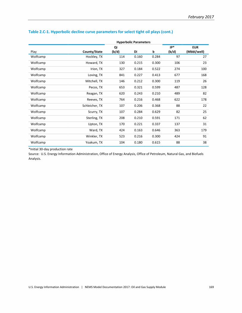
February 2017


Table 2.C-1. Hyperbolic decline curve parameters for select tight oil plays (cont.)


Play County/State Qi

(b/d) Di b IP*

(b/d) EUR

(Mbbl/well)

Wolfcamp Hockley, TX 114 0.160 0.284 97 27

Wolfcamp Howard, TX 130 0.215 0.300 106 23

Wolfcamp Irion, TX 327 0.184 0.522 274 100

Wolfcamp Loving, TX 841 0.227 0.413 677 168

Wolfcamp Mitchell, TX 146 0.212 0.300 119 26

Wolfcamp Pecos, TX 653 0.321 0.599 487 128

Wolfcamp Reagan, TX 620 0.243 0.210 489 82

Wolfcamp Reeves, TX 764 0.216 0.468 622 178

Wolfcamp Schleicher, TX 107 0.206 0.368 88 22

Wolfcamp Scurry, TX 107 0.284 0.629 82 25

Wolfcamp Sterling, TX 208 0.210 0.591 171 62

Wolfcamp Upton, TX 170 0.221 0.337 137 31

Wolfcamp Ward, TX 424 0.163 0.646 363 179

Wolfcamp Winkler, TX 523 0.216 0.300 424 91

Wolfcamp Yoakum, TX 104 0.180 0.615 88 38

*Initial 30-day production rate

Source: U.S. Energy Information Administration, Office of Energy Analysis, Office of Petroleum, Natural Gas, and Biofuels

Analysis.

February 2017


Table 2.C-2. Hyperbolic decline curve parameters for select shale gas plays

Play County/State

Hyperbolic Parameters IP*

(Mcf/d)

EUR

(MMcf/well) Qi

(Mcf/d) Di b

Barnett-Core Johnson, TX 3,238 0.407 1.312 2,337 1,623

Barnett-Core Tarrant, TX 2,578 0.138 1.097 2,267 2,196

Barnett-North Clay, TX 669 0.179 0.579 564 232

Barnett-North Cooke, TX 3,332 0.182 0.300 2,791 702

Barnett-North Denton, TX 1,953 0.161 1.381 1,688 1,889

Barnett-North Jack, TX 387 0.180 0.389 325 96

Barnett-North Wise, TX 1,293 0.125 1.318 1,152 1,397

Barnett-South Dallas, TX 2,548 0.125 1.138 2,267 2,405

Barnett-South Ellis, TX 1,894 0.211 1.197 1,569 1,319

Barnett-South Erath, TX 603 0.615 1.702 396 348

Barnett-South Hill, TX 1,583 0.353 1.638 1,198 1,180

Barnett-South Hood, TX 4,134 0.188 0.300 3,444 842

Barnett-South Montague, TX 1,172 0.186 0.993 988 718

Barnett-South Parker, TX 1,496 0.305 1.463 1,163 1,050

Barnett-South Shackelford, TX 138 0.230 0.273 110 21

Barnett-South Somervell, TX 1,184 0.436 1.472 845 673

Barnett-South Stephens, TX 312 0.249 0.357 245 51

Eagle Ford-Dry Bee, TX 2,313 0.081 0.213 2,135 1,032

Eagle Ford-Dry DeWitt, TX 3,968 0.116 0.273 3,540 1,321

Eagle Ford-Dry Karnes, TX 4,037 0.154 0.517 3,481 1,468

Eagle Ford-Dry Live Oak, TX 4,023 0.126 0.492 3,560 1,717

Eagle Ford-Dry Webb, TX 3,789 0.103 0.554 3,428 2,169

Eagle Ford-Wet Atascosa, TX 559 0.256 0.563 440 130

Eagle Ford-Wet Bee, TX 10,795 0.232 0.300 8,625 1,730

Eagle Ford-Wet DeWitt, TX 6,293 0.221 0.412 5,093 1,292

Eagle Ford-Wet Dimmit, TX 2,506 0.206 0.536 2,061 695

Eagle Ford-Wet Karnes, TX 3,213 0.229 0.398 2,580 618

Eagle Ford-Wet LaSalle, TX 2,795 0.224 0.440 2,258 595

Eagle Ford-Wet Lavaca, TX 1,771 0.465 0.637 1,178 252

Eagle Ford-Wet Live Oak, TX 4,456 0.228 0.468 3,589 981

Eagle Ford-Wet McMullen, TX 2,459 0.235 0.332 1,961 410

Eagle Ford-Wet Webb, TX 14,195 0.218 0.300 11,492 2,442

Eagle Ford-Wet Zavala, TX 380 0.205 0.424 312 87

Fayetteville-Central Cleburne, AR 2,680 0.161 1.059 2,309 1,968

Fayetteville-Central Conway, AR 3,036 0.167 1.118 2,605 2,306

Fayetteville-Central Faulkner, AR 3,143 0.226 1.104 2,567 1,883

Fayetteville-Central Independence, AR 1,619 0.126 0.859 1,437 1,159

Fayetteville-Central Jackson, AR 1,004 0.193 1.476 847 935

Fayetteville-Central Van Buren, AR 2,921 0.149 1.013 2,542 2,165

Fayetteville-Central White, AR 2,625 0.156 1.085 2,273 2,027

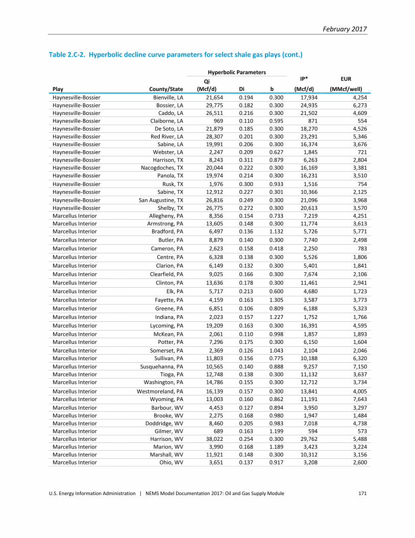
February 2017


Table 2.C-2. Hyperbolic decline curve parameters for select shale gas plays (cont.)

Play County/State


(Mcf/d)

EUR

(MMcf/well) Qi

(Mcf/d) Di b

Haynesville-Bossier Bienville, LA 21,654 0.194 0.300 17,934 4,254

Haynesville-Bossier Bossier, LA 29,775 0.182 0.300 24,935 6,273

Haynesville-Bossier Caddo, LA 26,511 0.216 0.300 21,502 4,609

Haynesville-Bossier Claiborne, LA 969 0.110 0.595 871 554

Haynesville-Bossier De Soto, LA 21,879 0.185 0.300 18,270 4,526

Haynesville-Bossier Red River, LA 28,307 0.201 0.300 23,291 5,346

Haynesville-Bossier Sabine, LA 19,991 0.206 0.300 16,374 3,676

Haynesville-Bossier Webster, LA 2,247 0.209 0.627 1,845 721

Haynesville-Bossier Harrison, TX 8,243 0.311 0.879 6,263 2,804

Haynesville-Bossier Nacogdoches, TX 20,044 0.222 0.300 16,169 3,381

Haynesville-Bossier Panola, TX 19,974 0.214 0.300 16,231 3,510

Haynesville-Bossier Rusk, TX 1,976 0.300 0.933 1,516 754

Haynesville-Bossier Sabine, TX 12,912 0.227 0.301 10,366 2,125

Haynesville-Bossier San Augustine, TX 26,816 0.249 0.300 21,096 3,968

Haynesville-Bossier Shelby, TX 26,775 0.272 0.300 20,613 3,570

Marcellus Interior Allegheny, PA 8,356 0.154 0.733 7,219 4,251

Marcellus Interior Armstrong, PA 13,605 0.148 0.300 11,774 3,613

Marcellus Interior Bradford, PA 6,497 0.136 1.132 5,726 5,771

Marcellus Interior Butler, PA 8,879 0.140 0.300 7,740 2,498

Marcellus Interior Cameron, PA 2,623 0.158 0.418 2,250 783

Marcellus Interior Centre, PA 6,328 0.138 0.300 5,526 1,806

Marcellus Interior Clarion, PA 6,149 0.132 0.300 5,401 1,841

Marcellus Interior Clearfield, PA 9,025 0.166 0.300 7,674 2,106

Marcellus Interior Clinton, PA 13,636 0.178 0.300 11,461 2,941

Marcellus Interior Elk, PA 5,717 0.213 0.600 4,680 1,723

Marcellus Interior Fayette, PA 4,159 0.163 1.305 3,587 3,773

Marcellus Interior Greene, PA 6,851 0.106 0.809 6,188 5,323

Marcellus Interior Indiana, PA 2,023 0.157 1.227 1,752 1,766

Marcellus Interior Lycoming, PA 19,209 0.163 0.300 16,391 4,595

Marcellus Interior McKean, PA 2,061 0.110 0.998 1,857 1,893

Marcellus Interior Potter, PA 7,296 0.175 0.300 6,150 1,604

Marcellus Interior Somerset, PA 2,369 0.126 1.043 2,104 2,046

Marcellus Interior Sullivan, PA 11,803 0.156 0.775 10,188 6,320

Marcellus Interior Susquehanna, PA 10,565 0.140 0.888 9,257 7,150

Marcellus Interior Tioga, PA 12,748 0.138 0.300 11,132 3,637

Marcellus Interior Washington, PA 14,786 0.155 0.300 12,712 3,734

Marcellus Interior Westmoreland, PA 16,139 0.157 0.300 13,841 4,005

Marcellus Interior Wyoming, PA 13,003 0.160 0.862 11,191 7,643

Marcellus Interior Barbour, WV 4,453 0.127 0.894 3,950 3,297

Marcellus Interior Brooke, WV 2,275 0.168 0.980 1,947 1,484

Marcellus Interior Doddridge, WV 8,460 0.205 0.983 7,018 4,738

Marcellus Interior Gilmer, WV 689 0.163 1.199 594 573

Marcellus Interior Harrison, WV 38,022 0.254 0.300 29,762 5,488

Marcellus Interior Marion, WV 3,990 0.168 1.189 3,423 3,224

Marcellus Interior Marshall, WV 11,921 0.148 0.300 10,312 3,156

Marcellus Interior Ohio, WV 3,651 0.137 0.917 3,208 2,600

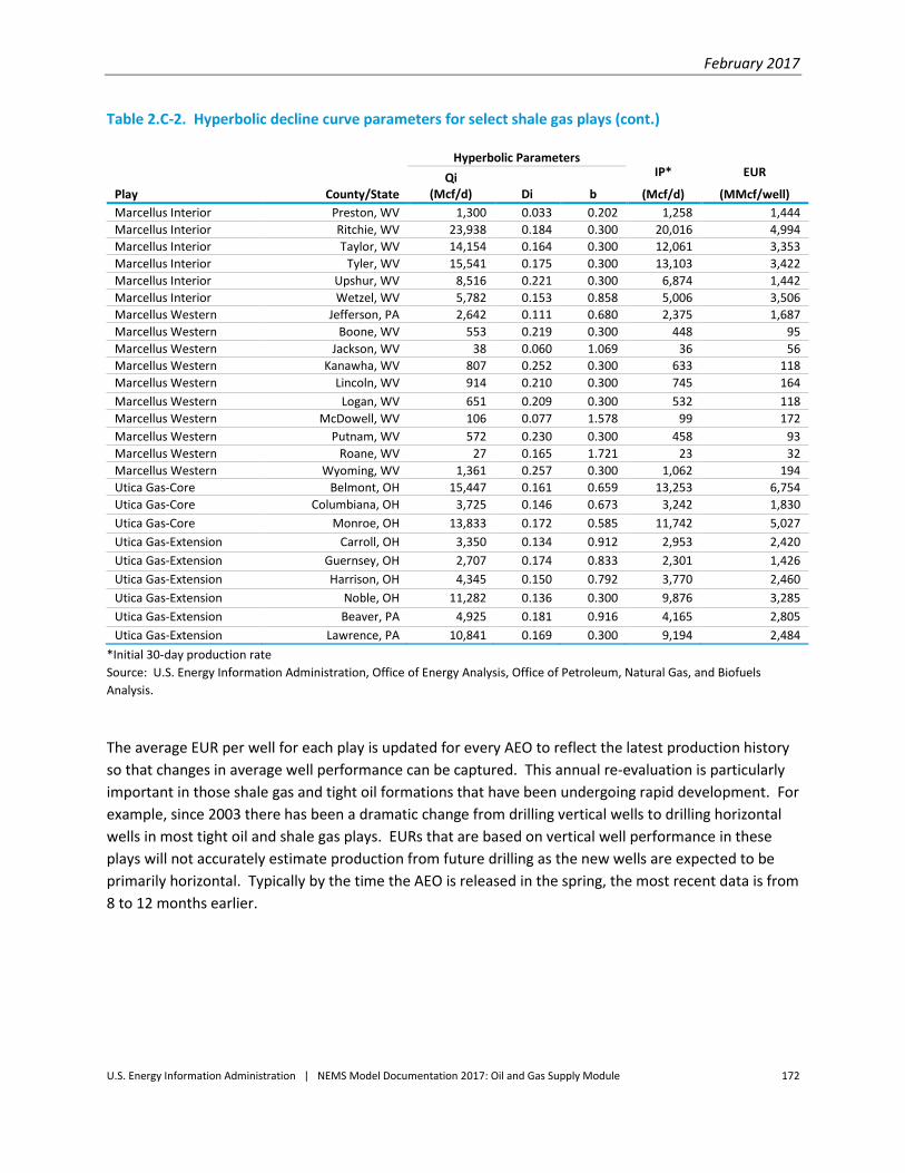
February 2017


Table 2.C-2. Hyperbolic decline curve parameters for select shale gas plays (cont.)

Play County/State


(Mcf/d)

EUR

(MMcf/well) Qi

(Mcf/d) Di b

Marcellus Interior Preston, WV 1,300 0.033 0.202 1,258 1,444

Marcellus Interior Ritchie, WV 23,938 0.184 0.300 20,016 4,994

Marcellus Interior Taylor, WV 14,154 0.164 0.300 12,061 3,353

Marcellus Interior Tyler, WV 15,541 0.175 0.300 13,103 3,422

Marcellus Interior Upshur, WV 8,516 0.221 0.300 6,874 1,442

Marcellus Interior Wetzel, WV 5,782 0.153 0.858 5,006 3,506

Marcellus Western Jefferson, PA 2,642 0.111 0.680 2,375 1,687

Marcellus Western Boone, WV 553 0.219 0.300 448 95

Marcellus Western Jackson, WV 38 0.060 1.069 36 56

Marcellus Western Kanawha, WV 807 0.252 0.300 633 118

Marcellus Western Lincoln, WV 914 0.210 0.300 745 164

Marcellus Western Logan, WV 651 0.209 0.300 532 118

Marcellus Western McDowell, WV 106 0.077 1.578 99 172

Marcellus Western Putnam, WV 572 0.230 0.300 458 93

Marcellus Western Roane, WV 27 0.165 1.721 23 32

Marcellus Western Wyoming, WV 1,361 0.257 0.300 1,062 194

Utica Gas-Core Belmont, OH 15,447 0.161 0.659 13,253 6,754

Utica Gas-Core Columbiana, OH 3,725 0.146 0.673 3,242 1,830

Utica Gas-Core Monroe, OH 13,833 0.172 0.585 11,742 5,027

Utica Gas-Extension Carroll, OH 3,350 0.134 0.912 2,953 2,420

Utica Gas-Extension Guernsey, OH 2,707 0.174 0.833 2,301 1,426

Utica Gas-Extension Harrison, OH 4,345 0.150 0.792 3,770 2,460

Utica Gas-Extension Noble, OH 11,282 0.136 0.300 9,876 3,285

Utica Gas-Extension Beaver, PA 4,925 0.181 0.916 4,165 2,805

Utica Gas-Extension Lawrence, PA 10,841 0.169 0.300 9,194 2,484

*Initial 30-day production rate


Analysis.

The average EUR per well for each play is updated for every AEO to reflect the latest production history

so that changes in average well performance can be captured. This annual re-evaluation is particularly

important in those shale gas and tight oil formations that have been undergoing rapid development. For

example, since 2003 there has been a dramatic change from drilling vertical wells to drilling horizontal

wells in most tight oil and shale gas plays. EURs that are based on vertical well performance in these

plays will not accurately estimate production from future drilling as the new wells are expected to be

primarily horizontal. Typically by the time the AEO is released in the spring, the most recent data is from

8 to 12 months earlier.

February 2017


Appendix 2.D: Representation of Power Plant and xTL Captured

CO2 in EOR

With the addition of the Capture, Transport, Utilization, and Storage (CTUS) Submodule and the revised

representation of CO2 enhanced oil recovery (EOR), the Electricity Market Module (EMM), Oil and Gas

Supply Module (OGSM), and Liquid Fuels Market Module (LFMM) were modified so that these models

all share a common vision of the market for CO2. The current representation of CO2 EOR better

integrates the EMM, OGSM, LFMM and CTUS.

When considering CO2 EOR, OGSM competes natural and industrial options for CO2 supply in a

given region against the availability and price of CO2 from power plants and xTL facilities6. OGSM

passes its resolution of the CO2 market to the EMM and LFMM.

The EMM considers as a part of its overall objective function retrofitting existing units or

building new generating units with CO2 capture to meet a new constraint of satisfying the total

CO2 demand passed from OGSM. Since EMM has the total picture as represented in OGSM, it

can determine the CO2 market size and competitive prices for CO2 captured from power

generators (including transport and storage costs provided by CTUS). The EMM then passes its

resolution of the CO2 market to OGSM and LFMM.

In a parallel fashion to the EMM, the LFMM considers as a part of its overall objective function

building (but not retrofitting) xTL facilities to meet a new constraint of satisfying the total CO2

demand passed from OGSM and EMM. Since LFMM has the total picture as represented in

OGSM, it can determine the CO2 market size and competitive prices for CO2 captured from xTL

facilities (including transport and storage costs provided by CTUS). The LFMM then passes its

resolution of the CO2 market to OGSM and LFMM.

This structure enables the model to dynamically solve for the capture of CO2 and the production of oil

from anthropogenic CO2 EOR.

OGSM generates the CO2 demand for EOR which it then shares with EMM and LFMM. EMM Electricity

Capacity Planning Module (ECP) and LFMM share the marginal cost (price) of CO2 supply with OGSM for

use in its selection of CO2 sources among competitive suppliers. Quantities of CO2 captured from EMM

and LFMM are also sent to CTUS for use in EOR and also for storage. CTUS calculates and shares the

cost of CO2 transportation and storage with both EMM and LFMM. Figure 2.D-1 illustrates the flow of

information among these modules.

To facilitate the flow of information between CTUS, EMM, OGSM and LFMM, several new variables were

introduced and are summarized in Table 2.D-1.

6 Generic designation for process converting anything to liquids, such as for gas-to-liquid (GTL), coal-to-liquid (CTL), and

Biomass-to-liquid (BTL).

February 2017


Figure 2.D-1. Flow of Information among EMM, LFMM, OGSM, and CTUS

EMM Data Shared CTUS Data Shared OGSM Data Shared LFMM Data Shared

CO2 supply (to OGSM) Cost of CO2 transport and

storage for power plants

(to EMM)

Competitive Market for

CO2/CO2 demand (to EMM)

CO2 supply (to OGSM)

CO2 price (to OGSM) Cost of CO2 transport

and storage for CTLs

(to LFMM)

Competitive Market for

CO2/CO2 demand (to

LFMM)

CO2 price (to OGSM)

CO2 capture for EOR and

Storage (to CTUS)

CO2 capture for EOR and

Storage (to CTUS)

February 2017


Table 2.D- 1. Inventory of Variables Passed Between CTUS, OGSM, EMM and LFMM

Variable Name Variable Type Description Units

OGCO2PUR2(8,13,MNUMYR)* Variable Volume of CO2 purchased. Same as OGCO2PUR but

organized by CO2 destination region.

MMcf

OGCO2PEM(8,MNUMYR) Variable CO2 price from EMM - 2nd year dual including

transport costs. These OGCO2PEM prices get loaded

into OGCO2PRC for power plants.

$/MMcf

OGCO2PLF(8,MNUMYR) Variable CO2 price from LFMM. These OGCO2PLF prices get

loaded into OGCO2PRC for xTL plants.

$/MMcf

OGCO2PRC(8,13,MNUMYR) Variable CO2 price by source. NOTE: Transport costs are not

included for industrial sources; transport IS included

for power plants and xTL plants.

$/MMcf

OGCO2QEM(8,MNUMYR) Variable CO2 quantity from EMM to OGSM. NOTE: 8th slot is

NOT the same definition - it is the extra CO2 that is

not sent to EOR but sent to saline storage, instead

(national basis).

MMcf

OGCO2QLF(8,MNUMYR) Variable CO2 quantity from LFMM. NOTE: 8th slot is NOT the

same definition - it is the extra CO2 that is not sent

to EOR but sent to saline storage, instead (national

basis).

MMcf

OGCO2TAR(8,8) Variable Transport price from OGSM for industrial sources. $/MMcf

*NOTE: For each of the variables, “8” refers to each of the 7 OGSM regions plus national; “13” refers to each of the CO2 source

technology options and “MNUMYR” refers to the year in which the activity takes place.

Modification of EOR project constraints in OGSM In OGSM, the number of new EOR project starts in a given year is constrained as a function of the

amount of excess captured CO2 (i.e. CO2 that is captured, but not used for EOR in that year) and is

expressed as

co2cap = oit_wop(curiyr,1) * 0.02 + (oOGCO2QEM(8,curiyr) * 0.001 + oOGCO2AVL(8,11,curiyr) * 0.001) * 0.05,

where

co2cap = maximum number of EOR projects starts in a given year; oit_wop(curiyr,1) = world oil price; oOGCO2QEM(8,curiyr) = CO2 captured from power plants, but not sent to EOR; and oOGCO2AVL (8,11,itimeyr) = CO2 captured from CTLs, but not sent to EOR.

February 2017


Integration of EMM into CO2 EOR process The EMM represents power plants with CO2 capture. These facilities capture CO2 and send it to either

EOR or saline storage. With the addition of the CTUS model, the EMM was modified so that the NEMS

OGSM model, the NEMS LFMM model, and the EMM all share a common vision of the market for CO2

capture, transportation, and storage. To that end, the EMM is given the following:

1. The EOR demand for CO2 by NEMS OGSM region

2. The prices for purchased CO2 from sources other than power plants (such as xTL facilities)

3. The cost of transporting CO2 from EMM fuel regions to OGSM regions (from CTUS)

4. The cost of transporting CO2 between OGSM regions

The EMM returns the following:

1. The amount of captured CO2 from power plants used to satisfy EOR demand in each OGSM

region

2. The additional amount of captured CO2 from power plants that is available to satisfy EOR

demands (in Carbon Constrained scenarios EMM may capture CO2 and send it to saline storage)

3. The marginal price of CO2 from power plants

Mathematical description of EMM-CTUS constraints The mathematical representation of the CO2 capture constraints in EMM are described below.

Definition of sets and parameters:

1. 𝑂 ≡ Set of NEMS OGSM regions

2. 𝐹 ≡ Set of NEMS EMM fuel regions

3. 𝑆 ≡ Set of CO2 sources

4. 𝐷𝑂 ≡ Demand for CO2 from EOR sites in OGSM region (O)

5. 𝑃𝑂,𝑆 ≡ CO2 production cost in OGSM region (O) from CO2 source (S)

6. 𝑇𝑂,𝑂′ ≡ CO2 transportation cost from OGSM region (O) to OGSM region (O’)

7. 𝑇𝐹,𝑂 ≡ CO2 transportation cost from fuel region (F) to OGSM region (O) for use in EOR

8. 𝑇𝑆𝐹,𝑂 ≡ CO2 transportation and storage cost from fuel region (F) to OGSM region (O) for

injection into a saline storage site

9. 𝐴𝑂,𝑆 ≡ Quantity of available CO2 for OGSM region (O) from CO2 source (S)

10. 𝐶𝑂2_𝐶𝐴𝑃 ≡ Quantity of CO2 captured per unit of electricity produced

Definition of decision variables:

1. 𝐸𝑀𝑀_𝑂𝑃𝐹 = Operation level of power plants fuel region (F)

2. 𝐸𝑀𝑀_𝐸𝑂𝑅𝐹,𝑂 = Amount of CO2 captured from the operation of power plants in fuel region (F)

and transported to OGSM region (O) for use in EOR

3. 𝐸𝑀𝑀_𝑆𝐴𝐿𝐹 = Amount of CO2 captured from the operation of power plants in fuel region (F)

and transported for injection into saline sites

4. 𝐶𝑂2_𝑇𝑅𝐴𝑁𝑂,𝑂′ = Amount of CO2 transported from OGSM region (O) to OGSM region (O’) for

use in EOR from non-power plant sources

February 2017


5. 𝐶𝑂2_𝑃𝑈𝑅𝐶𝐻𝑂,𝑆 = Amount of CO2 purchased in OGSM region (O) from CO2 source (S)

Definition of the constraints:

1. OGSM EOR demand for CO2 must be satisfied in each OGSM region (O):

The amount of CO2 transported into OGSM region (O) from all other OGSM regions plus the

amount of CO2 transported into this OGSM region from power plants plus the amount of CO2

purchased from xTL sources7 in this OGSM region must equal the EOR CO2 demand in this OGSM

region.

∑ 𝐶𝑂2_𝑇𝑅𝐴𝑁𝑂,𝑂′

𝑂

+ ∑ 𝐸𝑀𝑀_𝐸𝑂𝑅𝐹,𝑂

𝐹

+ 𝐶𝑂2_𝑃𝑈𝑅𝐶𝐻𝑂,𝑆(𝑥𝑇𝐿) − 𝐷𝑂 = 0

2. CO2 that is purchased in each OGSM region (O) from sources other than from power plants or

xTLs in each OGSM region (O) must be transported before it can be used to satisfy EOR

demands.

∑ 𝐶𝑂2_𝑃𝑈𝑅𝐶𝐻𝑂,𝑆

𝑆≠𝑝𝑜𝑤𝑒𝑟 𝑜𝑟 𝑋𝑇𝐿

− ∑ 𝐶𝑂2_𝑇𝑅𝐴𝑁𝑂,𝑂′

𝑂′

= 0

3. CO2 that is captured from power plants in each fuel region (F) must be must either be sent to

EOR or saline injection in carbon constrained scenarios.

𝐶𝑂2𝐶𝐴𝑃 ∗ 𝐸𝑀𝑀 − ∑ 𝐸𝑀𝑀_𝐸𝑂𝑅𝐹,𝑂

𝑂

− 𝐸𝑀𝑀_𝑆𝐴𝐿𝐹 = 0

Otherwise, the amount of CO2 captured must exceed the amount shipped to EOR.

𝐶𝑂2𝐶𝐴𝑃 ∗ 𝐸𝑀𝑀 − ∑ 𝐸𝑀𝑀_𝐸𝑂𝑅𝐹,𝑂

𝑂

− 𝐸𝑀𝑀_𝑆𝐴𝐿𝐹 ≥ 0

4. The amount of CO2 that is purchased from source (S) in each OGSM region (O) is limited to the

amount available.

𝐶𝑂2_𝑃𝑈𝑅𝐶𝐻𝑂,𝑆 ≤ 𝐴𝑂,𝑆

Integration of LFMM into CO2 EOR process The LFMM has process representations of coal-to-liquids and coal+biomass-to-liquids facilities, which

may capture CO2 and send it to either EOR or saline storage. With the addition of the CTUS model, the

LFMM was modified so that the NEMS OGSM model, the NEMS EMM model, and the LFMM all share a

7 Note that the ‘CO2_PURCH’ variable here is only for xTL sources since the purchase prices for CO2 that come from the LFMM

are delivered costs, so no transportation cost component needs to be added.

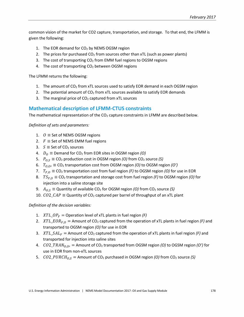
February 2017


common vision of the market for CO2 capture, transportation, and storage. To that end, the LFMM is

given the following:

1. The EOR demand for CO2 by NEMS OGSM region

2. The prices for purchased CO2 from sources other than xTL (such as power plants)

3. The cost of transporting CO2 from EMM fuel regions to OGSM regions

4. The cost of transporting CO2 between OGSM regions

The LFMM returns the following:

1. The amount of CO2 from xTL sources used to satisfy EOR demand in each OGSM region

2. The potential amount of CO2 from xTL sources available to satisfy EOR demands

3. The marginal price of CO2 captured from xTL sources

Mathematical description of LFMM-CTUS constraints The mathematical representation of the CO2 capture constraints in LFMM are described below.

Definition of sets and parameters:

1. 𝑂 ≡ Set of NEMS OGSM regions

2. 𝐹 ≡ Set of NEMS EMM fuel regions

3. 𝑆 ≡ Set of CO2 sources

4. 𝐷𝑂 ≡ Demand for CO2 from EOR sites in OGSM region (O)

5. 𝑃𝑂,𝑆 ≡ CO2 production cost in OGSM region (O) from CO2 source (S)

6. 𝑇𝑂,𝑂′ ≡ CO2 transportation cost from OGSM region (O) to OGSM region (O’)

7. 𝑇𝐹,𝑂 ≡ CO2 transportation cost from fuel region (F) to OGSM region (O) for use in EOR

8. 𝑇𝑆𝐹,𝑂 ≡ CO2 transportation and storage cost from fuel region (F) to OGSM region (O) for

injection into a saline storage site

9. 𝐴𝑂,𝑆 ≡ Quantity of available CO2 for OGSM region (O) from CO2 source (S)

10. 𝐶𝑂2_𝐶𝐴𝑃 ≡ Quantity of CO2 captured per barrel of throughput of an xTL plant

Definition of the decision variables:

1. 𝑋𝑇𝐿_𝑂𝑃𝐹 = Operation level of xTL plants in fuel region (F)

2. 𝑋𝑇𝐿_𝐸𝑂𝑅𝐹,𝑂 = Amount of CO2 captured from the operation of xTL plants in fuel region (F) and

transported to OGSM region (O) for use in EOR

3. 𝑋𝑇𝐿_𝑆𝐴𝐿𝐹 = Amount of CO2 captured from the operation of xTL plants in fuel region (F) and

transported for injection into saline sites

4. 𝐶𝑂2_𝑇𝑅𝐴𝑁𝑂,𝑂′ = Amount of CO2 transported from OGSM region (O) to OGSM region (O’) for

use in EOR from non-xTL sources

5. 𝐶𝑂2_𝑃𝑈𝑅𝐶𝐻𝑂,𝑆 = Amount of CO2 purchased in OGSM region (O) from CO2 source (S)

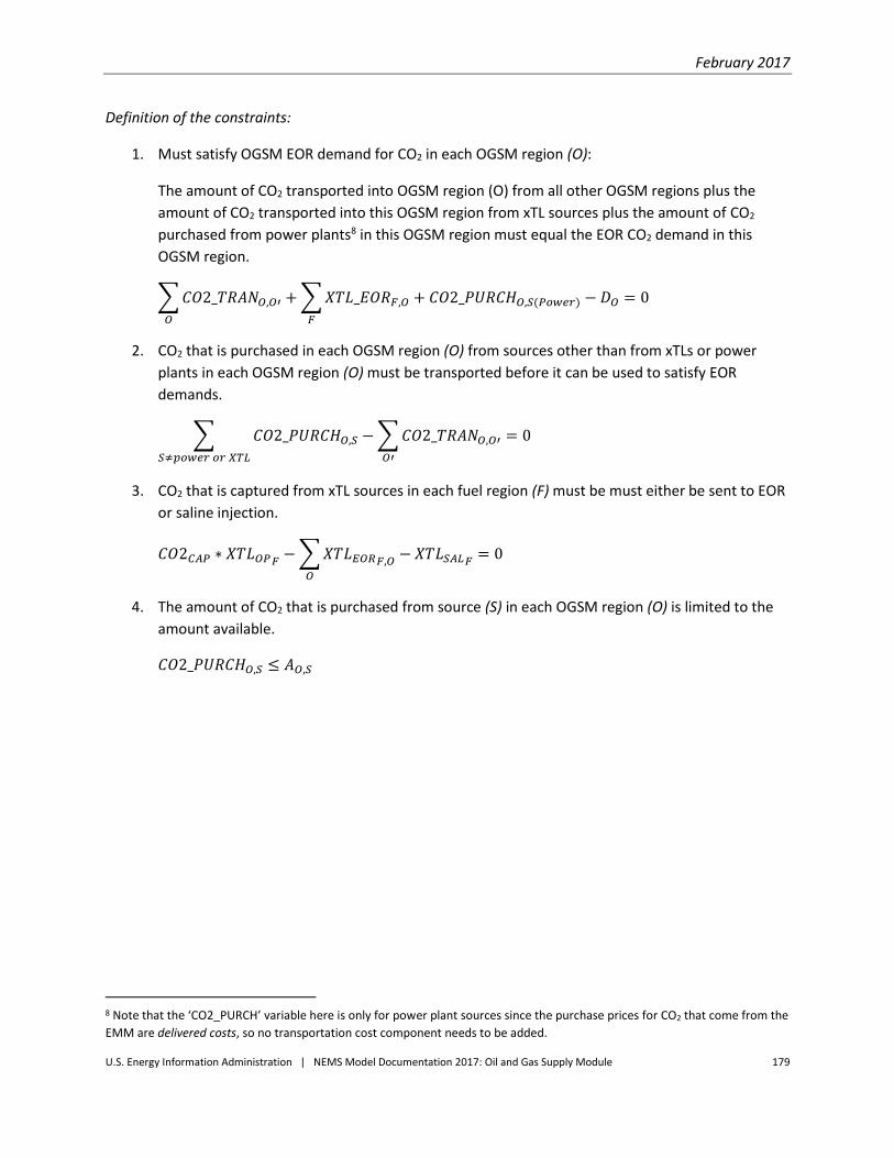
February 2017


Definition of the constraints:

1. Must satisfy OGSM EOR demand for CO2 in each OGSM region (O):

The amount of CO2 transported into OGSM region (O) from all other OGSM regions plus the

amount of CO2 transported into this OGSM region from xTL sources plus the amount of CO2

purchased from power plants8 in this OGSM region must equal the EOR CO2 demand in this

OGSM region.

∑ 𝐶𝑂2_𝑇𝑅𝐴𝑁𝑂,𝑂′

𝑂

+ ∑ 𝑋𝑇𝐿_𝐸𝑂𝑅𝐹,𝑂

𝐹

+ 𝐶𝑂2_𝑃𝑈𝑅𝐶𝐻𝑂,𝑆(𝑃𝑜𝑤𝑒𝑟) − 𝐷𝑂 = 0

2. CO2 that is purchased in each OGSM region (O) from sources other than from xTLs or power

plants in each OGSM region (O) must be transported before it can be used to satisfy EOR

demands.

∑ 𝐶𝑂2_𝑃𝑈𝑅𝐶𝐻𝑂,𝑆

𝑆≠𝑝𝑜𝑤𝑒𝑟 𝑜𝑟 𝑋𝑇𝐿

− ∑ 𝐶𝑂2_𝑇𝑅𝐴𝑁𝑂,𝑂′

𝑂′

= 0

3. CO2 that is captured from xTL sources in each fuel region (F) must be must either be sent to EOR

or saline injection.

𝐶𝑂2𝐶𝐴𝑃 ∗ 𝑋𝑇𝐿𝑂𝑃𝐹− ∑ 𝑋𝑇𝐿𝐸𝑂𝑅𝐹,𝑂

𝑂

− 𝑋𝑇𝐿𝑆𝐴𝐿𝐹= 0

4. The amount of CO2 that is purchased from source (S) in each OGSM region (O) is limited to the

amount available.

𝐶𝑂2_𝑃𝑈𝑅𝐶𝐻𝑂,𝑆 ≤ 𝐴𝑂,𝑆

8 Note that the ‘CO2_PURCH’ variable here is only for power plant sources since the purchase prices for CO2 that come from the

EMM are delivered costs, so no transportation cost component needs to be added.

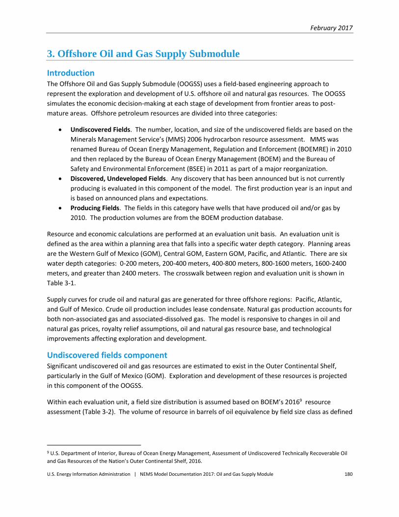
February 2017


3. Offshore Oil and Gas Supply Submodule

Introduction The Offshore Oil and Gas Supply Submodule (OOGSS) uses a field-based engineering approach to

represent the exploration and development of U.S. offshore oil and natural gas resources. The OOGSS

simulates the economic decision-making at each stage of development from frontier areas to post-

mature areas. Offshore petroleum resources are divided into three categories:

Undiscovered Fields. The number, location, and size of the undiscovered fields are based on the

Minerals Management Service’s (MMS) 2006 hydrocarbon resource assessment. MMS was

renamed Bureau of Ocean Energy Management, Regulation and Enforcement (BOEMRE) in 2010

and then replaced by the Bureau of Ocean Energy Management (BOEM) and the Bureau of

Safety and Environmental Enforcement (BSEE) in 2011 as part of a major reorganization.

Discovered, Undeveloped Fields. Any discovery that has been announced but is not currently

producing is evaluated in this component of the model. The first production year is an input and

is based on announced plans and expectations.

Producing Fields. The fields in this category have wells that have produced oil and/or gas by

2010. The production volumes are from the BOEM production database.

Resource and economic calculations are performed at an evaluation unit basis. An evaluation unit is

defined as the area within a planning area that falls into a specific water depth category. Planning areas

are the Western Gulf of Mexico (GOM), Central GOM, Eastern GOM, Pacific, and Atlantic. There are six

water depth categories: 0-200 meters, 200-400 meters, 400-800 meters, 800-1600 meters, 1600-2400

meters, and greater than 2400 meters. The crosswalk between region and evaluation unit is shown in

Table 3-1.

Supply curves for crude oil and natural gas are generated for three offshore regions: Pacific, Atlantic,

and Gulf of Mexico. Crude oil production includes lease condensate. Natural gas production accounts for

both non-associated gas and associated-dissolved gas. The model is responsive to changes in oil and

natural gas prices, royalty relief assumptions, oil and natural gas resource base, and technological

improvements affecting exploration and development.

Undiscovered fields component Significant undiscovered oil and gas resources are estimated to exist in the Outer Continental Shelf,

particularly in the Gulf of Mexico (GOM). Exploration and development of these resources is projected

in this component of the OOGSS.

Within each evaluation unit, a field size distribution is assumed based on BOEM’s 20169 resource

assessment (Table 3-2). The volume of resource in barrels of oil equivalence by field size class as defined

9 U.S. Department of Interior, Bureau of Ocean Energy Management, Assessment of Undiscovered Technically Recoverable Oil

and Gas Resources of the Nation’s Outer Continental Shelf, 2016.

February 2017


by BOEM is shown in Table 3-3. In the OOGSS, the mean estimate represents the size of each field in the

field size class. Water depth and field size class are used for specifying many of the technology

assumptions in the OOGSS. Fields smaller than field size class 2 are assumed to be uneconomic to

develop.

Table 3-1. Offshore region and evaluation unit crosswalk

No. Region Name Planning Area

Water Depth

(meters)

Drilling Depth

(feet)

Evaluation

Unit Name Region ID

1 Shallow GOM Western GOM 0 - 200 < 15,000 WGOM0002 3

2 Shallow GOM Western GOM 0 - 200 > 15,000 WGOMDG02 3

3 Deep GOM Western GOM 201 - 400 All WGOM0204 4

4 Deep GOM Western GOM 401 - 800 All WGOM0408 4

5 Deep GOM Western GOM 801 - 1,600 All WGOM0816 4

6 Deep GOM Western GOM 1,601 - 2,400 All WGOM1624 4

7 Deep GOM Western GOM > 2,400 All WGOM2400 4

8 Shallow GOM Central GOM 0 - 200 < 15,000 CGOM0002 3

9 Shallow GOM Central GOM 0 - 200 > 15,000 CGOMDG02 3

10 Deep GOM Central GOM 201 - 400 All CGOM0204 4

11 Deep GOM Central GOM 401 - 800 All CGOM0408 4

12 Deep GOM Central GOM 801 - 1,600 All CGOM0816 4

13 Deep GOM Central GOM 1,601 – 2,400 All CGOM1624 4

14 Deep GOM Central GOM > 2,400 All CGOM2400 4

15 Shallow GOM Eastern GOM 0 - 200 All EGOM0002 3

16 Deep GOM Eastern GOM 201 - 400 All EGOM0204 4

17 Deep GOM Central GOM 401 - 800 All EGOM0408 4



20 Deep GOM Eastern GOM > 2400 All EGOM2400 4

21 Deep GOM Eastern GOM > 200 All EGOML181 4

22 Atlantic North Atlantic 0 - 200 All NATL0002 1

23 Atlantic North Atlantic 201 - 800 All NATL0208 1

24 Atlantic North Atlantic > 800 All NATL0800 1

25 Atlantic Mid Atlantic 0 - 200 All MATL0002 1

26 Atlantic Mid Atlantic 201 - 800 All MATL0208 1

27 Atlantic Mid Atlantic > 800 All MATL0800 1

28 Atlantic South Atlantic 0 - 200 All SATL0002 1

29 Atlantic South Atlantic 201 - 800 All SATL0208 1

30 Atlantic South Atlantic > 800 All SATL0800 1

31 Atlantic Florida Straits 0 – 200 All FLST0002 1

February 2017


Table 3-1. Offshore Region and Evaluation Unit Crosswalk (cont.)

No. Region Name Planning Area

Water Depth

(meters)

Drilling Depth

(feet)

Evaluation

Unit Name Region ID

32 Atlantic Florida Straits 201 - 800 All FLST0208 1

33 Atlantic Florida Straits > 800 All FLST0800 1

34 Pacific Pacific Northwest 0-200 All PNW0002 2

35 Pacific Pacific Northwest 201-800 All PNW0208 2

36 Pacific North California 0-200 All NCA0002 2




40 Pacific Central California 0-200 All CCA0002 2



43 Pacific South California 0-200 All SCA0002 2





Analysis.

February 2017


Table 3-2. Number of undiscovered fields by evaluation unit and field size class, as of 1/1/2014

Evaluation

Unit

Field Size Class Number

of Fields

Total

Resource

(BBOE) 2 3 4 5 6 7 8 9 10 11 12 13 14 15 16 17

WGOM0002 11 19 27 39 38 38 34 25 13 9 3 4 2 1 0 0 268 3558

WGOMDG02 6 10 14 19 19 19 17 13 7 4 2 2 1 0 0 0 135 1801

WGOM0204 0 0 0 1 2 2 3 4 4 3 2 1 0 0 0 0 23 842

WGOM0408 0 0 1 1 2 3 5 6 6 5 3 2 1 0 0 0 34 1263

WGOM0816 0 1 2 5 10 15 24 29 29 22 15 7 3 1 0 0 163 6530

WGOM1624 0 0 1 2 3 5 8 9 10 8 5 3 2 0 0 0 56 2450

WGOM2400 0 0 0 1 2 3 5 5 6 5 3 2 1 0 0 0 33 1439

CGOM0002 16 29 41 57 58 57 55 45 20 12 6 5 3 1 0 0 412 4917

CGOMDG02 9 15 22 30 30 30 28 24 11 7 3 2 1 0 0 0 215 2567

CGOM0204 0 0 1 2 4 5 9 12 12 9 6 2 1 0 0 0 64 2403

CGOM0408 0 1 1 2 5 8 14 19 19 14 8 4 1 1 0 0 96 3604

CGOM0816 1 2 4 9 17 26 46 62 63 48 31 14 5 2 0 0 330 13105

CGOM1624 1 2 3 7 14 23 39 50 54 41 29 14 6 2 1 0 286 13962

CGOM2400 0 1 1 3 7 13 22 29 31 25 18 10 4 2 1 0 167 9927

EGOM0002 4 6 7 8 8 8 7 5 4 2 2 2 0 0 0 0 66 857

EGOM0204 1 2 2 2 2 3 2 1 0 0 0 0 0 0 0 0 18 174

EGOM0408 2 2 3 4 4 4 3 2 1 1 1 1 0 0 0 0 27 260

EGOM0816 1 1 2 2 2 3 2 2 1 1 0 0 0 0 0 0 17 116

EGOM1624 0 0 0 0 0 0 1 1 1 0 0 0 0 0 0 0 3 40

EGOM2400 0 0 1 1 4 6 9 12 13 11 7 5 2 1 0 0 72 3921

EGOML181 0 0 0 0 0 0 0 0 0 0 0 0 0 0 0 0 0 0

NATL0002 0 0 0 0 1 2 2 5 6 3 1 1 0 0 0 0 21 614

NATL0208 0 0 0 0 1 1 1 3 4 2 1 1 0 0 0 0 14 492

NATL0800 0 0 0 0 1 2 3 4 5 5 4 3 1 1 0 0 29 2346

MATL0002 0 0 0 0 1 2 2 2 2 2 1 1 0 0 0 0 13 443

MATL0208 0 0 0 0 2 3 3 3 3 3 2 1 1 0 0 0 21 980

MATL0800 0 0 0 0 2 4 6 8 10 10 9 7 4 1 0 0 61 4980

SATL0002 0 0 0 0 0 0 0 0 0 0 0 0 0 0 0 0 0 0

SATL0208 0 0 0 0 2 3 3 2 2 1 0 0 0 0 0 0 13 143

SATL0800 0 0 0 0 5 6 6 5 4 3 1 1 0 0 0 0 31 609

PNW0002 10 17 24 29 27 20 13 8 4 2 1 0 0 0 0 0 160 572

PNW0208 4 6 9 10 10 7 5 3 2 1 0 0 0 0 0 0 59 202

NCA0002 1 2 3 5 5 5 5 4 3 2 1 1 0 0 0 0 37 526

NCA0208 9 17 24 28 26 21 14 9 5 3 1 1 0 0 0 0 162 833

NCA0816 3 6 9 12 12 11 9 7 5 3 2 1 0 0 0 0 81 801

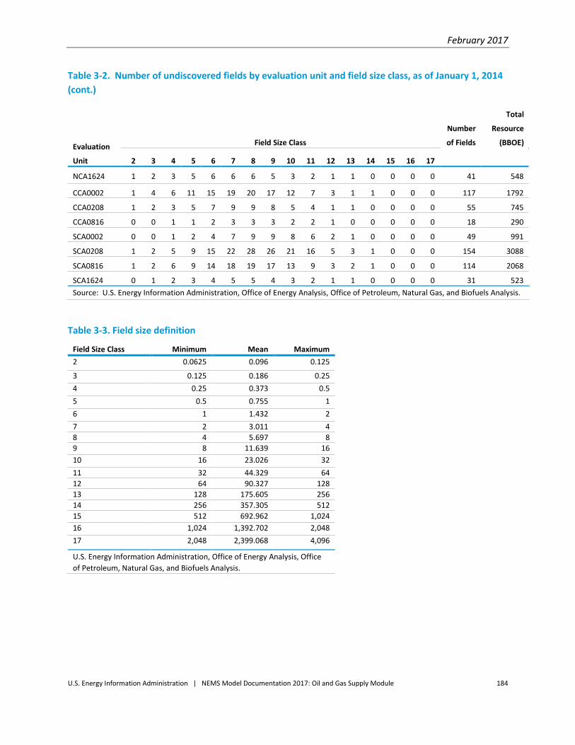
February 2017


Table 3-2. Number of undiscovered fields by evaluation unit and field size class, as of January 1, 2014

(cont.)

Evaluation

Unit

Field Size Class

Number

of Fields

Total

Resource

(BBOE)

2 3 4 5 6 7 8 9 10 11 12 13 14 15 16 17

NCA1624 1 2 3 5 6 6 6 5 3 2 1 1 0 0 0 0 41 548

CCA0002 1 4 6 11 15 19 20 17 12 7 3 1 1 0 0 0 117 1792

CCA0208 1 2 3 5 7 9 9 8 5 4 1 1 0 0 0 0 55 745

CCA0816 0 0 1 1 2 3 3 3 2 2 1 0 0 0 0 0 18 290

SCA0002 0 0 1 2 4 7 9 9 8 6 2 1 0 0 0 0 49 991

SCA0208 1 2 5 9 15 22 28 26 21 16 5 3 1 0 0 0 154 3088

SCA0816 1 2 6 9 14 18 19 17 13 9 3 2 1 0 0 0 114 2068

SCA1624 0 1 2 3 4 5 5 4 3 2 1 1 0 0 0 0 31 523

Source: U.S. Energy Information Administration, Office of Energy Analysis, Office of Petroleum, Natural Gas, and Biofuels Analysis.

Table 3-3. Field size definition

Field Size Class Minimum Mean Maximum

2 0.0625 0.096 0.125

3 0.125 0.186 0.25

4 0.25 0.373 0.5

5 0.5 0.755 1

6 1 1.432 2

7 2 3.011 4

8 4 5.697 8

9 8 11.639 16

10 16 23.026 32

11 32 44.329 64

12 64 90.327 128

13 128 175.605 256

14 256 357.305 512

15 512 692.962 1,024

16 1,024 1,392.702 2,048

17 2,048 2,399.068 4,096

U.S. Energy Information Administration, Office of Energy Analysis, Office

of Petroleum, Natural Gas, and Biofuels Analysis.

February 2017


Projection of discoveries

The number and size of discoveries is projected based on a simple model developed by J. J. Arps and T.

G. Roberts in 1958.10 For a given evaluation unit in the OOGSS, the number of cumulative discoveries for

each field size class is determined by

DiscoveredFields TotalFields *(1 e )EU,iFSC EU,iFSC

*CumNFWEU,iFSC EU

(3-1)

where

TotalFields = Total number of fields by evaluation unit and field size class

CumNFW = Cumulative new field wildcats drilled in an evaluation unit

γ = search coefficient

EU = evaluation unit

iFSC = field size class.

The search coefficient (γ) was chosen to make Equation 3-1 fit the data. In many cases, however, the

sparse exploratory activity in an evaluation unit made fitting the discovery model problematic. To

provide reasonable estimates of the search coefficient in every evaluation unit, the data in various field

size classes within a region were grouped as needed to obtain enough data points to provide a

reasonable fit to the discovery model. A polynomial was fit to all of the relative search coefficients in

the region. The polynomial was fit to the resulting search coefficients as follows:

EU,iFSC2

EU,101*iFSC + 2*iFSC + 3* (3-2)

where

β1 = 0.0243 for Western GOM and 0.0399 for Central and Eastern GOM

β2 = -0.3525 for Western GOM and -0.6222 for Central and Eastern GOM

β3 = 1.5326 for Western GOM and 2.2477 for Central and 3.0477 for Eastern GOM

iFSC = field size class

γ = search coefficient for field size class 10.

Cumulative new field wildcat drilling is determined by

CumNFW CumNFW 1 *(OILPRICE *GASPRICE )EU,t EU,t 1 EU EU t nlag1 t nlag2 (3-3)

10Arps, J. J. and T. G. Roberts, Economics of Drilling for Cretaceous Oil on the East Flank of the Denver-Julesburg Basin,

Bulletin of the American Association of Petroleum Geologists, November 1958.

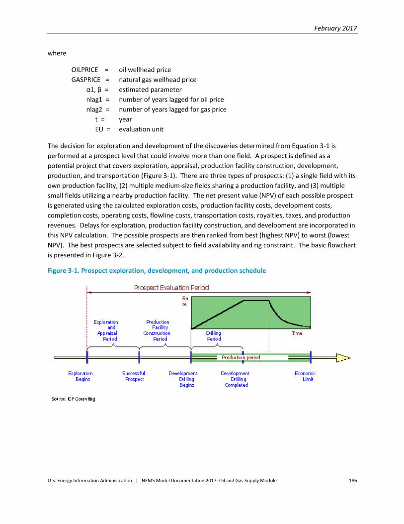
February 2017


where

OILPRICE = oil wellhead price

GASPRICE = natural gas wellhead price

α1, β = estimated parameter

nlag1 = number of years lagged for oil price

nlag2 = number of years lagged for gas price

t = year

EU = evaluation unit

The decision for exploration and development of the discoveries determined from Equation 3-1 is

performed at a prospect level that could involve more than one field. A prospect is defined as a

potential project that covers exploration, appraisal, production facility construction, development,

production, and transportation (Figure 3-1). There are three types of prospects: (1) a single field with its

own production facility, (2) multiple medium-size fields sharing a production facility, and (3) multiple

small fields utilizing a nearby production facility. The net present value (NPV) of each possible prospect

is generated using the calculated exploration costs, production facility costs, development costs,

completion costs, operating costs, flowline costs, transportation costs, royalties, taxes, and production

revenues. Delays for exploration, production facility construction, and development are incorporated in

this NPV calculation. The possible prospects are then ranked from best (highest NPV) to worst (lowest

NPV). The best prospects are selected subject to field availability and rig constraint. The basic flowchart

is presented in Figure 3-2.

Figure 3-1. Prospect exploration, development, and production schedule

February 2017


Figure 3-2. Flowchart for the Undiscovered Field Component of the OOGSS

Calculation of costs

The technology employed in the deepwater offshore areas to find and develop hydrocarbons can be

significantly different than that used in shallower waters, and represents significant challenges for the

companies and individuals involved in the deepwater development projects. In many situations in the

deepwater Outer Continental Shelf (OCS), the choice of technology used in a particular situation

depends on the size of the prospect being developed. The following base costs are adjusted with the oil

price to capture the variation in costs over time as activity level and demand for equipment and other

supplies change. The adjustment factor is [0.6 + (oilprice/baseprice)], where baseprice = $75/barrel.

Exploration drilling

During the exploration phase of an offshore project, the type of drilling rig used depends on both

economic and technical criteria. Offshore exploratory drilling usually is done using self-contained rigs

that can be moved easily. Three types of drilling rigs are incorporated into the OOGSS. The exploration

drilling costs per well for each rig type are a function of water depth (WD) and well drilling depth (DD),

both in feet.

February 2017


Jack-up rigs are limited to a water depth of about 600 feet or less. Jack-ups are towed to their location,

where heavy machinery is used to jack the legs down into the water until they rest on the ocean floor.

When this is completed, the platform containing the work area rises above the water. After the

platform has risen about 50 feet out of the water, the rig is ready to begin drilling.

ExplorationDrillingCosts($/well) = 2,000,000 + (5.0E-09)*WD*DD3 (3-4)

Semi-submersible rigs are floating structures that employ large engines to position the rig over the hole

dynamically. This extends the maximum operating depth greatly, and some of these rigs can be used in

water depths up to and beyond 3,000 feet. The shape of a semisubmersible rig tends to dampen wave

motion greatly regardless of wave direction. This allows its use in areas where wave action is severe.

ExplorationDrillingCosts($/well) = 2,500,000 + 400*WD + 200*(WD+DD) + (2.0E-05)*WD*DD2 (3-5)

Dynamically positioned drill ships are a second type of floating vessel used in offshore drilling. They are

usually used in water depths exceeding 3,000 feet where the semi-submersible type of drilling rigs

cannot be deployed. Some of the drillships are designed with the rig equipment and anchoring system

mounted on a central turret. The ship is rotated about the central turret using thrusters so that the ship

always faces incoming waves. This helps to dampen wave motion.

ExplorationDrillingCosts($/well) = 7,500,000 + (1.0E-05)*WD*DD2 (3-6)

Water depth is the primary criterion for selecting a drilling rig. Drilling in shallow waters (up to 1,500

feet) can be done with jack-up rigs. Drilling in deeper water (greater than 1,500 feet) can be done with

semi-submersible drilling rigs or drill ships. The number of rigs available for exploration is limited and

varies by water depth levels. Drilling rigs are allowed to move one water depth level lower if needed.

Production and development structure

Six different options for development/production of offshore prospects are currently assumed in

OOGSS, based on those currently considered and/or employed by operators in the Gulf of Mexico OCS.

These are conventional fixed platforms, compliant towers, tension leg platforms, spar platforms, floating

production systems and subsea satellite well systems. Choice of platform tends to be a function of the

size of field and water depth, though in reality other operational, environmental, and/or economic

decisions influence the choice. Production facility costs are a function of water depth (WD) and number

of slots per structure (SLT).

Conventional fixed platform (FP). A fixed platform consists of a jacket with a deck placed on top, providing space for crew quarters, drilling rigs, and production facilities. The jacket is a tall vertical section made of tubular steel members supported by piles driven into the seabed. The fixed platform is economical for installation in water depths up to 1,200 feet. Although advances in engineering design and materials have been made, these structures are not economically feasible in deeper waters.

StructureCost($) 2,000,000 9,000*SLT 1,500*WD*SLT + 40*WD2 (3-7)

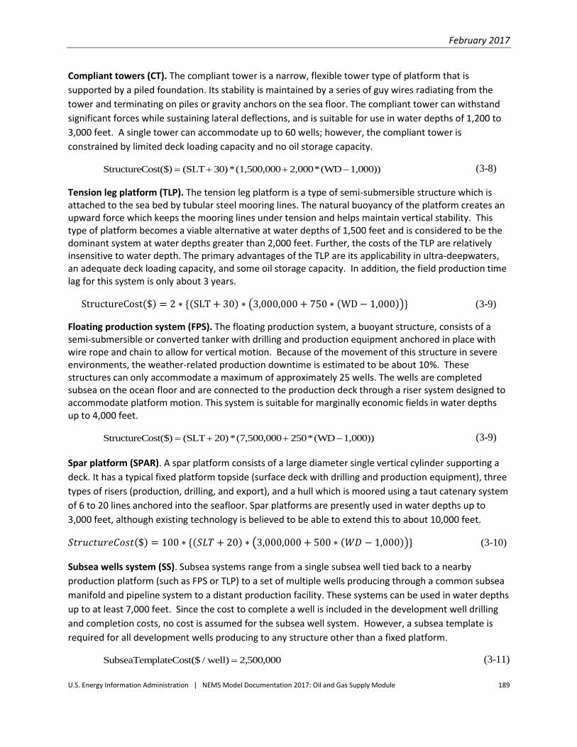
February 2017


Compliant towers (CT). The compliant tower is a narrow, flexible tower type of platform that is

supported by a piled foundation. Its stability is maintained by a series of guy wires radiating from the

tower and terminating on piles or gravity anchors on the sea floor. The compliant tower can withstand

significant forces while sustaining lateral deflections, and is suitable for use in water depths of 1,200 to

3,000 feet. A single tower can accommodate up to 60 wells; however, the compliant tower is

constrained by limited deck loading capacity and no oil storage capacity.

StructureCost($) (SLT 30)*(1,500,000 2,000*(WD 1,000)) (3-8)

Tension leg platform (TLP). The tension leg platform is a type of semi-submersible structure which is attached to the sea bed by tubular steel mooring lines. The natural buoyancy of the platform creates an upward force which keeps the mooring lines under tension and helps maintain vertical stability. This type of platform becomes a viable alternative at water depths of 1,500 feet and is considered to be the dominant system at water depths greater than 2,000 feet. Further, the costs of the TLP are relatively insensitive to water depth. The primary advantages of the TLP are its applicability in ultra-deepwaters, an adequate deck loading capacity, and some oil storage capacity. In addition, the field production time lag for this system is only about 3 years.

StructureCost($) = 2 ∗ {(SLT + 30) ∗ (3,000,000 + 750 ∗ (WD − 1,000))} (3-9)

Floating production system (FPS). The floating production system, a buoyant structure, consists of a semi-submersible or converted tanker with drilling and production equipment anchored in place with wire rope and chain to allow for vertical motion. Because of the movement of this structure in severe environments, the weather-related production downtime is estimated to be about 10%. These structures can only accommodate a maximum of approximately 25 wells. The wells are completed subsea on the ocean floor and are connected to the production deck through a riser system designed to accommodate platform motion. This system is suitable for marginally economic fields in water depths up to 4,000 feet.

StructureCost($) (SLT *(7,500,000 *(WD 1,000)) 20) 250 (3-9)

Spar platform (SPAR). A spar platform consists of a large diameter single vertical cylinder supporting a

deck. It has a typical fixed platform topside (surface deck with drilling and production equipment), three

types of risers (production, drilling, and export), and a hull which is moored using a taut catenary system

of 6 to 20 lines anchored into the seafloor. Spar platforms are presently used in water depths up to

3,000 feet, although existing technology is believed to be able to extend this to about 10,000 feet.

𝑆𝑡𝑟𝑢𝑐𝑡𝑢𝑟𝑒𝐶𝑜𝑠𝑡($) = 100 ∗ {(𝑆𝐿𝑇 + 20) ∗ (3,000,000 + 500 ∗ (𝑊𝐷 − 1,000))} (3-10)

Subsea wells system (SS). Subsea systems range from a single subsea well tied back to a nearby

production platform (such as FPS or TLP) to a set of multiple wells producing through a common subsea

manifold and pipeline system to a distant production facility. These systems can be used in water depths

up to at least 7,000 feet. Since the cost to complete a well is included in the development well drilling

and completion costs, no cost is assumed for the subsea well system. However, a subsea template is

required for all development wells producing to any structure other than a fixed platform.

SubseaTemplateCost($ / well) 2 500 000, , (3-11)

February 2017


The type of production facility for development and production depends on water depth level as shown

in Table 3-4.

Table 3-4. Production facility by water depth level

Minimum Maximum FP CT TLP FPS SPAR SS

0 656 X X

656 2625

X

X

2625 5249

X

X

5249 7874

X X X

7874 10000

X X X

Source: ICF Consulting.

Development drilling

Pre-drilling of development wells during the platform construction phase is done using the drilling rig

employed for exploration drilling. Development wells drilled after installation of the platform which also

serves as the development structure are done using the platform itself. Hence, the choice of drilling rig

for development drilling is tied to the choice of the production platform.

For water depths less than or equal to 900 meters,

DevelopmentDrillingCost ($

well) = 5 ∗ {1,500,000 + (1,500 + 0.04 ∗ DD) ∗ WD

+(0.035 ∗ 𝐷𝐷 − 300) ∗ 𝐷𝐷} (3-13)

For water depths greater than 900 meters,

DevelopmentDrillingCost ($

well) = 5 ∗ {4,500,000 + (150 + 0.004 ∗ DD) ∗ WD

+(0.035 ∗ 𝐷𝐷 − 250) ∗ 𝐷𝐷} (3-14)

where

WD = water depth in feet

DD = drilling depth in feet.

Completion and operating

Completion costs per well are a function of water depth range and drilling depth as shown in Table 3-5.

February 2017


Table 3-5. Well completion and equipment costs per well

Water Depth (feet)

Development Drilling Depth (feet)

< 10,000 10,001 - 20,000 > 20,000

0 - 3,000 800,000 2,100,000 3,300,000

> 3,000 1,900,000 2,700,000 3,300,000

Platform operating costs for all types of structures are assumed to be a function of water depth (WD)

and the number of slots (SLT). These costs include the following items:

primary oil and gas production costs

labor

communications and safety equipment

supplies and catering services

routine process and structural maintenance

well service and workovers

insurance on facilities

transportation of personnel and supplies

Annual operating costs are estimated by

OperatingCost($/structure/year) = 3 ∗ (1,265,000 + 135,000 ∗ SLT + 0.0588 ∗ SLT ∗ WD2) (3-12)

Transportation

It is assumed in the model that existing trunk pipelines will be used and that the prospect economics

must support only the gathering system design and installation. However, in case of small fields tied

back to some existing neighboring production platform, a pipeline is assumed to be required to

transport the crude oil and natural gas to the neighboring platform.

Structure and facility abandonment

The costs to abandon the development structure and production facilities depend on the type of

production technology used. The model projects abandonment costs for fixed platforms and compliant

towers assuming that the structure is abandoned. It projects costs for tension leg platforms, converted

semi-submersibles, and converted tankers assuming that the structures are removed for transport to

another location for reinstallation. These costs are treated as intangible capital investments and are

expensed in the year following cessation of production. Based on historical data, these costs are

estimated as a fraction of the initial structure costs, as follows:

February 2017


Fraction of Initial Platform Cost

Fixed Platform 0.10

Compliant Tower 0.10

Tension Leg Platform 0.10

Floating Production Systems 0.10

Spar Platform 0.10

Exploration, development, and production scheduling

The typical offshore project development consists of the following phases: 11

Exploration phase

Exploration drilling program

Delineation drilling program

Development phase

Fabrication and installation of the development/production platform

Development drilling program

Pre-drilling during construction of platform

Drilling from platform

Construction of gathering system

Production operations

Field abandonment

The timing of each activity, relative to the overall project life and to other activities, affects the potential

economic viability of the undiscovered prospect. The modeling objective is to develop an exploration,

development, and production plan which both realistically portrays existing and/or anticipated offshore

practices and also allows for the most economical development of the field. A description of each of the

phases is provided below.

Exploration phase

An undiscovered field is assumed to be discovered by a successful exploration well (i.e., a new field

wildcat). Delineation wells are then drilled to define the vertical and areal extent of the reservoir.

Exploration drilling. The exploration success rate (ratio of the number of field discovery wells to total

wildcat wells) is used to establish the number of exploration wells required to discover a field as follows:

number of exploratory wells = 1/ [exploration success rate]

11 The pre-development activities, including early field evaluation using conventional geological and geophysical methods and

the acquisition of the right to explore the field, are assumed to be completed before initiation of the development of the

prospect.

February 2017


For example, a 25% exploration success rate will require four exploratory wells: one of the four wildcat

wells drilled finds the field and the other three are dry holes.

Delineation drilling. Exploratory drilling is followed by delineation drilling for field appraisal (1 to 4 wells

depending on the size of the field). The delineation wells define the field location vertically and

horizontally so that the development structures and wells may be set in optimal positions. All

delineation wells are converted to production wells at the end of the production facility construction.

Development phase

During this phase of an offshore project, the development structures are designed, fabricated, and

installed; the development wells (successful and dry) are drilled and completed; and the product

transportation/gathering system is installed.

Development structures. The model assumes that the design and construction of any development

structure begins in the year following completion of the exploration and delineation drilling program.

However, the length of time required to complete the construction and installation of these structures

depends on the type of system used. The required time for construction and installation of the various

development structures used in the model is shown in Table 3-6. This time lag is important in all

offshore developments, but it is especially critical for fields in deepwater and for marginally economic

fields.

Development drilling schedule. The number of development wells varies by water depth and field size

class as follows.

DevelopmentWells5

FSC * FSIZE DepthClass

(3-13)

where

FSC = field size class

FSIZE = resource volume (MMBOE)

β = 0.8 for water depths < 200 meters; 0.7 for water depths 200-800 meters; 0.65 for

water depths > 800 meters.

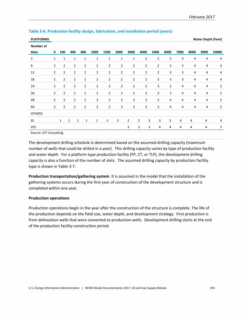
February 2017


Table 3-6. Production facility design, fabrication, and installation period (years)

PLATFORMS Water Depth (Feet)

Number of

Slots

0

100

400

800

1000

1500

2000

3000

4000

5000

6000

7000

8000

9000

10000

2 1 1 1 1 1 1 1 1 2 2 3 3 4 4 4

8 2 2 2 2 2 2 2 2 2 2 3 3 4 4 4

12 2 2 2 2 2 2 2 2 2 2 3 3 4 4 4

18 2 2 2 2 2 2 2 2 2 3 3 3 4 4 4

24 2 2 2 2 2 2 2 2 2 3 3 4 4 4 5

36 2 2 2 2 2 2 2 2 2 3 3 4 4 4 5

48 2 2 2 2 2 2 3 3 3 3 4 4 4 4 5

60 2 2 2 2 2 2 3 3 3 3 4 4 4 4 5

OTHERS

SS 1 1 1 1 1 1 2 2 2 3 3 3 4 4 4 4

FPS

3 3 3 4 4 4 4 4 5


The development drilling schedule is determined based on the assumed drilling capacity (maximum

number of wells that could be drilled in a year). This drilling capacity varies by type of production facility

and water depth. For a platform type production facility (FP, CT, or TLP), the development drilling

capacity is also a function of the number of slots. The assumed drilling capacity by production facility

type is shown in Table 3-7.

Production transportation/gathering system. It is assumed in the model that the installation of the

gathering systems occurs during the first year of construction of the development structure and is

completed within one year.

Production operations

Production operations begin in the year after the construction of the structure is complete. The life of

the production depends on the field size, water depth, and development strategy. First production is

from delineation wells that were converted to production wells. Development drilling starts at the end

of the production facility construction period.

February 2017


Table 3-7. Development drilling capacity by production facility type

Maximum Number of Wells Drilled

(wells/platform/year, 1 rig)

Maximum Number of Wells Drilled

(wells/field/year)

Drilling Depth (feet) Drilling Capacity (24 slots) Water Depth

(feet) SS FPS FPSO

0 24 0 4

4

6,000 24 1,000 4

4

7,000 24 2,000 4

4

8,000 20 3,000 4 4 4

9,000 20 4,000 4 4 4

10,000 20 5,000 3 3 3

11,000 20 6,000 2 2 2

12,000 16 7,000 2 2 2

13,000 16 8,000 1 1 1

14,000 12 9,000 1 1 1

15,000 8 10,000 1 1 1

16,000 4

17,000 2

18,000 2

19,000 2

20,000 2

30,000 2


Production profiles

The original hydrocarbon resource (in BOE) is divided between oil and natural gas using a user-specified

proportion. Due to the development drilling schedule, not all wells in the same field will produce at the

same time. This yields a ramp-up profile in the early production period (Figure 3-3). The initial

production rate is the same for all wells in the field and is constant for a period of time. Field production

reaches its peak when all the wells have been drilled and start producing. The production will start to

decline (at a user-specified rate) when the ratio of cumulative production to initial resource equals a

user-specified fraction.

Gas (plus lease condensate) production is calculated based on gas resource, and oil (plus associated-

dissolved gas) production is calculated based on the oil resource. Lease condensate production is

separated from the gas production using the user-specified condensate yield. Likewise, associated-

dissolved gas production is separated from the oil production using the user-specified associated gas-to-

February 2017


oil ratio. Associated-dissolved gas production is then tracked separately from the non-associated gas

production throughout the projection. Lease condensate production is added to crude oil production

and is not tracked separately.

Figure 3-3. Undiscovered field production profile

Field abandonment

All wells in a field are assumed to be shut in when the net revenue from the field is less than total state

and federal taxes. Net revenue is total revenue from production less royalties, operating costs,

transportation costs, and severance taxes.

Discovered undeveloped fields component Announced discoveries that have not been brought into production by 2002 are included in this

component of the OOGSS. The data required for these fields include location, field size class, gas

percentage of BOE resource, condensate yield, gas-to-oil ratio, start year of production, initial

production rate, fraction produced before decline, and hyperbolic decline parameters. The BOE

resource for each field corresponds to the field size class as specified in Table 3-3.

The number of development wells is the same as that of an undiscovered field in the same water depth

and of the same field size class (Equation 3-13). The production profile is also the same as that of an

undiscovered field (Figure 3-3).

The assumed field size and year of initial production of the major announced deepwater discoveries that

were not brought into production by 2009 are shown in Table 3-8. A field that is announced as an oil

field is assumed to be 100% oil and a field that is announced as a gas field is assumed to be 100% gas. If

a field is expected to produce both oil and gas, 70% is assumed to be oil and 30% is assumed to be gas.

February 2017


Table 3-8. Assumed size and initial production year of major announced deepwater discoveries

Field/Project Name Block

Water

Depth

(feet)

Year of

Discovery

Field Size

Class

Field Size

(MMBoe)

Start Year of

Production

GOTCHA AC865 7,844 2006 12 90 2019

VICKSBURG DC353 7,457 2009 14 357 2019

BUSHWOOD GB506 2,700 2009 12 90 2019

SAMURAI GC432 3,400 2009 12 90 2017

STAMPEDE-PONY GC468 3,497 2006 14 357 2018

STAMPEDE-KNOTTY HEAD GC512 3,557 2005 14 357 2018

HEIDELBERG GC903 5,271 2009 14 357 2016

TIBER KC102 4,132 2009 15 692 2017

KASKIDA KC292 5,894 2006 15 692 2020

MOCCASIN KC736 6,759 2011 14 357 2021

BUCKSKIN KC872 6,978 2009 13 176 2018

HADRIAN NORTH KC919 7,000 2010 14 357 2020

DIAMOND LL370 9,975 2008 10 23 2018

CHEYENNE EAST LL400 9,187 2011 9 12 2020

MANDY MC199 2,478 2010 13 176 2020

APPOMATTOX MC392 7,290 2009 13 176 2017

DEIMOS SOUTH MC762 3,122 2010 12 90 2016

KODIAK MC771 5,006 2008 13 176 2018

WEST BOREAS MC792 3,094 2009 12 90 2016

VITO MC984 4,038 2009 13 176 2020

KAIKIAS MC768 4,575 2014 12 90 2024

BIG FOOT WR029 5,235 2006 13 176 2018

SHENANDOAH WR052 5,750 2009 15 692 2017

STONES WR508 9,556 2005 12 90 2018

JULIA WR627 7,087 2007 12 90 2016

GUNFLINT MC948 6,138 2008 12 90 2016

GILA KC093 4,900 2013 13 176 2017

AMETHYST MC026 1,200 2014 11 45 2017

RYDBERG MC525 7,500 2014 12 90 2019

SON OF BLUTO 2 MC431 6,461 2012 11 45 2017

NORTH PLATTE GB959 4,400 2012 13 176 2022

PARMER GC823 3,821 2012 11 45 2022

PHOBOS SE039 8,500 2013 12 90 2018

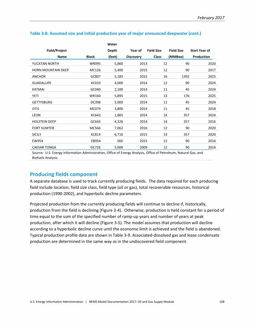
February 2017


Table 3-8. Assumed size and initial production year of major announced deepwater (cont.)

Field/Project

Name Block

Water

Depth

(feet)

Year of

Discovery

Field Size

Class

Field Size

(MMBoe)

Start Year of

Production

YUCATAN NORTH WR095 5,860 2013 12 90 2020

HORN MOUNTAIN DEEP MC126 5,400 2015 12 90 2017

ANCHOR GC807 5,183 2015 16 1392 2025

GUADALUPE KC010 4,000 2014 12 90 2024

KATMAI GC040 2,100 2014 11 45 2024

YETI WR160 5,895 2015 13 176 2025

GETTYSBURG DC398 5,000 2014 11 45 2024

OTIS MC079 3,800 2014 11 45 2018

LEON KC642 1,865 2014 14 357 2024

HOLSTEIN DEEP GC643 4,326 2014 14 357 2016

FORT SUMTER MC566 7,062 2016 12 90 2020

SICILY KC814 6,716 2015 14 357 2020

EW954 EB954 560 2015 12 90 2016

CAESAR TONGA GC726 5,000 2009 12 90 2016

Source: U.S. Energy Information Administration, Office of Energy Analysis, Office of Petroleum, Natural Gas, and

Biofuels Analysis.

Producing fields component A separate database is used to track currently producing fields. The data required for each producing

field include location, field size class, field type (oil or gas), total recoverable resources, historical

production (1990-2002), and hyperbolic decline parameters.

Projected production from the currently producing fields will continue to decline if, historically,

production from the field is declining (Figure 3-4). Otherwise, production is held constant for a period of

time equal to the sum of the specified number of ramp-up years and number of years at peak

production, after which it will decline (Figure 3-5). The model assumes that production will decline

according to a hyperbolic decline curve until the economic limit is achieved and the field is abandoned.

Typical production profile data are shown in Table 3-9. Associated-dissolved gas and lease condensate

production are determined in the same way as in the undiscovered field component.

February 2017


Figure 3-4. Production profile for producing fields − constant production case

Figure 3-5. Production profile for producing fields − declining production case

Table 3-9. Production profile data for oil & gas producing fields

Crude Oil Natural Gas

FSC 2 – 10 FSC 11 - 17 FSC 2 - 10 FSC 11 - 17

Ramp-up

(years)

At Initial Decline

Rate

Ramp-up

(years)

At Initial Decline

Rate

Ramp-up

(years)

At Initial Decline

Rate

Ramp-up

(years)

At Initial Decline

Rate Peak

(years) Peak

(years) Peak

(years) Peak

(years)

Shallow GOM

2 1 0.15 3 4 0.1 2 1 0.3 3 2 0.3

Deep GOM

2 2 0.15 2 4 0.1 2 1 0.3 3 2 0.3

Atlantic 2 1 0.15 3 3 0.15 2 1 0.3 3 2 0.3

Pacific 2 1 0.1 3 2 0.1 2 1 0.3 3 2 0.1

FSC = Field Size Class


February 2017


Generation of supply curves As mentioned earlier, the OOGSS does not determine the actual volume of crude oil and non-associated

natural gas produced in a given projection year, but rather provides the parameters for the short-term

supply functions used to determine regional supply and demand market equilibration. For each year, t,

and offshore region, r, the OGSM calculates the stock of proved reserves at the beginning of year t+1

and the expected production-to-reserves (PR) ratio for year t+1 as follows.

The volume of proved reserves in any year is calculated as

REVOFF + NRDOFF + PRDOFF - RESOFF = RESOFF tk,r,tk,r,tk,r,tk,r,1t+k,r, (3-14)

where

RESOFF = beginning- of-year reserves PRDOFF = production NRDOFF = new reserve discoveries REVOFF = reserve extensions, revisions, and adjustments r = region (1=Atlantic, 2=Pacific, 3=GOM) k = fuel type (1=oil; 2=non-associated gas) t = year.

Expected production, EXPRDOFF, is the sum of the field-level production determined in the

undiscovered fields component, the discovered, undeveloped fields component, and the producing field

component. The volume of crude oil production (including lease condensate), PRDOFF, passed to the

LFMM is equal to EXPRDOFF. Non-associated natural gas production in year t is the market-equilibrated

volume passed to the OGSM from the NGTDM.

Reserves are added through new field discoveries as well as delineation and developmental drilling.

Each newly discovered field not only adds proved reserves but also a much larger amount of inferred

reserves. The allocation between proved and inferred reserves is based on historical reserves growth

statistics. Specifically,

RSVGRO

1 * NFDISC = NRDOFF

k

1t-k,r,tk,r, (3-15)

RSVGRO

1 - 1 * NFDISC = NIRDOFF

k

1t-k,r,tk,r, (3-16)

where

NRDOFF = new reserve discovery

NIRDOFF = new inferred reserve additions

NFDISC = new field discoveries

RSVGRO = reserves growth factor (8.2738 for oil and 5.9612 for gas)

r = region (1=Atlantic, 2=Pacific, 3=GOM)

February 2017


k = fuel type (1=oil; 2=gas)

t = year.

Reserves are converted from inferred to proved with the drilling of other exploratory (or delineation)

wells and developmental wells. Since the expected offshore PR ratio is assumed to remain constant at

the last historical value, the reserves needed to support the total expected production, EXPRDOFF, can

be calculated by dividing EXPRDOFF by the PR ratio. Solving Equation 3-1 for REVOFFr,k,t and writing

RESOFFr,k,t+1=EXPRDOFFr,k,t+1

PRr,k⁄

gives

NRDOFF - RESOFF - PRDOFF + PR

EXPRDOFF = REVOFF tk,r,tk,r,tk,r,

kr,

1tk,r,

tk,r,

(3-17)

The remaining proved reserves, inferred reserves, and undiscovered resources are tracked throughout

the projection period to ensure that production from offshore sources does not exceed the assumed

resource base. Field-level associated-dissolved gas is summed to the regional level and passed to the

NGTDM.

Advanced technology impacts Advances in technology for the various activities associated with crude oil and natural gas exploration,

development, and production can have a profound impact on the costs associated with these activities.

The OOGSS has been designed to give due consideration to the effect of advances in technology that

may occur in the future. The specific technology levers and values are presented in Table 3-10.

Table 3-10. Offshore exploration and production technology levers

Technology Level Total Improvement

(percent) Number of Years

Delay to commence first exploration and between exploration 15 30

Exploration & development drilling costs 30 30

Operating cost 30 30

Time to construct production facility 15 30

Production facility construction costs 30 30

Initial constant production rate 15 30

Decline rate 0 30


February 2017


Appendix 3.A. Offshore data inventory

VARIABLES

Variable Name

Description Unit Classification Code Text

ADVLTXOFF PRODTAX Offshore ad valorem tax rates Fraction 4 Lower 48 offshore subregions;

Fuel (oil, gas)

CPRDOFF COPRD Offshore coproduct rate Fraction 4 Lower 48 offshore subregions;

Fuel (oil, gas)

CUMDISC DiscoveredFields Cumulative number of

discovered offshore fields

NA Offshore evaluation unit: Field

size class

CUMNFW CumNFW Cumulative number of new

fields wildcats drilled

NA Offshore evaluation unit: Field

size class

CURPRROFF omega Offshore initial P/R ratios Fraction 4 Lower 48 offshore subregions;

Fuel (oil, gas)

CURRESOFF R Offshore initial reserves MMbbl

Bcf

4 Lower 48 offshore subregions;

Fuel (oil, gas)

DECLOFF -- Offshore decline rates Fraction 4 Lower 48 offshore subregions;

Fuel (oil, gas)

DEVLCOST DevelopmentDrilli

ngCost

Development drilling cost $ per well Offshore evaluation unit

DRILLOFF DRILL Offshore drilling cost 1987$ 4 Lower 48 offshore subregions

DRYOFF DRY Offshore dry hole cost 1987$ Class (exploratory,

developmental);

4 Lower 48 offshore subregions

DVWELLOFF -- Offshore development project

drilling schedules

wells per year 4 Lower 48 offshore subregions;

Fuel (oil, gas)

ELASTOFF --

Offshore production elasticity

values

Fraction 4 Lower 48 offshore subregions

EXPLCOST ExplorationDrilling

Costs

Exploration well drilling cost $ per well Offshore evaluation unit

EXWELLOFF -- Offshore exploratory project

drilling schedules

wells per year 4 Lower 48 offshore subregions

FLOWOFF -- Offshore flow rates bbls, Mcf per

year


Fuel (oil, gas)

FRMINOFF FRMIN Offshore minimum exploratory

well finding rate

MMbbl

Bcf

per well


Fuel (oil, gas)

February 2017


VARIABLES

Variable Name

Code Text Description Unit Classification

FR1OFF FR1

FR2OFF FR3 Offshore developmental

well finding rate

MMbbl

Bcf

per well


Fuel (oil, gas)

FR3OFF FR2 Offshore other exploratory

well finding rate

MMbbl

Bcf

per well


Fuel (oil, gas)

HISTPRROFF -- Offshore historical P/R ratios fraction 4 Lower 48 offshore subregions;

Fuel (oil, gas)

HISTRESOFF -- Offshore historical

beginning-of-year reserves

MMbbl

Bcf


Fuel (oil, gas)

INFRSVOFF I Offshore inferred reserves MMbbl

Bcf


Fuel (oil, gas)

KAPFRCOFF EXKAP Offshore drill costs that are

tangible & must be

depreciated

fraction Class (exploratory, developmental)

KAPSPNDOFF KAP Offshore other capital

expenditures

1987$ Class (exploratory,

developmental);


LEASOFF EQUIP Offshore lease equipment

cost

1987$ per

project

Class (exploratory,

developmental);


NDEVWLS DevelopmentWells Number of development

wells drilled

NA Offshore evaluation unit

NFWCOSTOFF COSTEXP Offshore new field wildcat

cost


developmental);


NFWELLOFF -- Offshore exploratory and

developmental project

drilling schedules

wells per project

per year

Class (exploratory,

developmental);

r=1

NIRDOFF NIRDOFF Offshore new inferred

reserves

Oil-MMbbl per

well

Gas-Bcf per well

Offshore region; Offshore

fuel(oil,gas)

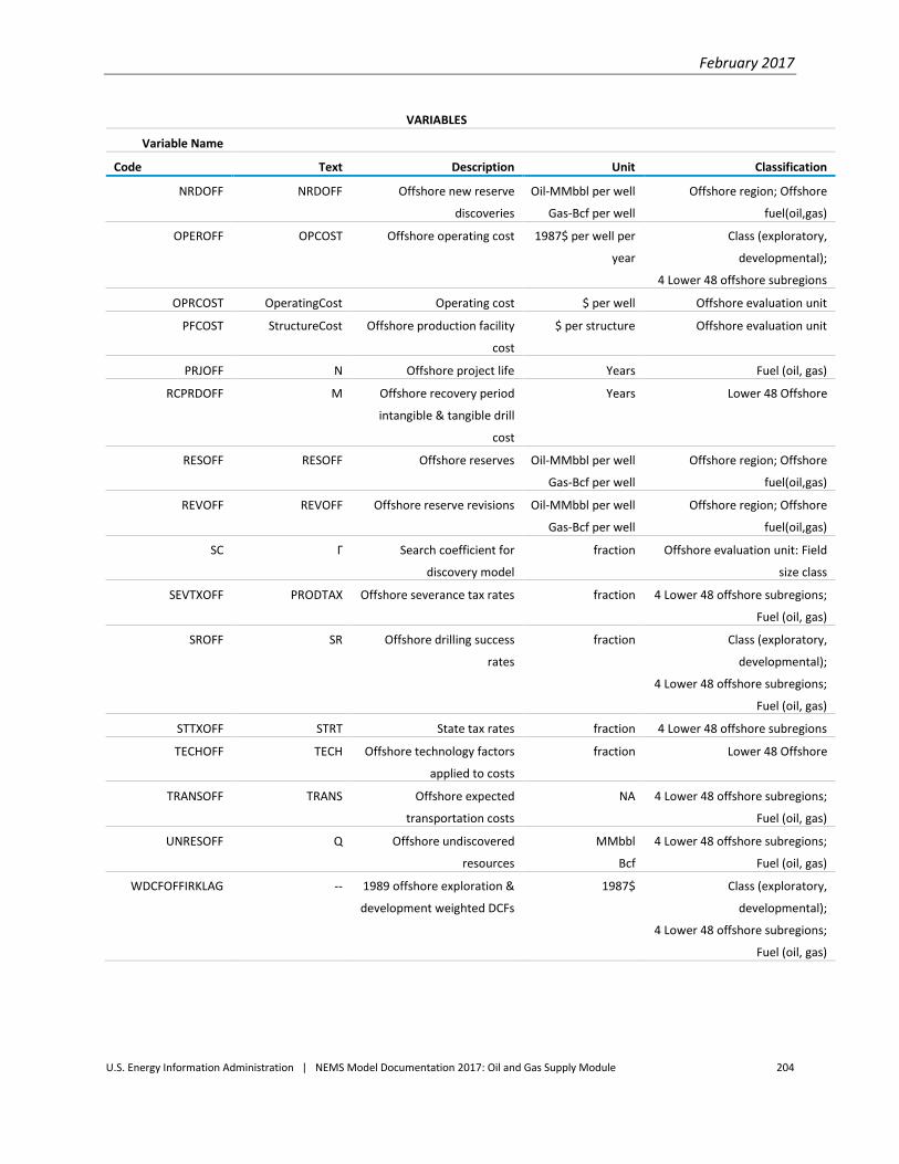
February 2017


VARIABLES

Variable Name


NRDOFF NRDOFF Offshore new reserve

discoveries

Oil-MMbbl per well

Gas-Bcf per well


fuel(oil,gas)

OPEROFF OPCOST Offshore operating cost 1987$ per well per

year

Class (exploratory,

developmental);


OPRCOST OperatingCost Operating cost $ per well Offshore evaluation unit

PFCOST StructureCost Offshore production facility

cost

$ per structure Offshore evaluation unit

PRJOFF N Offshore project life Years Fuel (oil, gas)

RCPRDOFF M Offshore recovery period

intangible & tangible drill

cost

Years Lower 48 Offshore

RESOFF RESOFF Offshore reserves Oil-MMbbl per well

Gas-Bcf per well


fuel(oil,gas)

REVOFF REVOFF Offshore reserve revisions Oil-MMbbl per well

Gas-Bcf per well


fuel(oil,gas)

SC Γ Search coefficient for

discovery model

fraction Offshore evaluation unit: Field

size class

SEVTXOFF PRODTAX Offshore severance tax rates fraction 4 Lower 48 offshore subregions;

Fuel (oil, gas)

SROFF SR Offshore drilling success

rates

fraction Class (exploratory,

developmental);


Fuel (oil, gas)

STTXOFF STRT State tax rates fraction 4 Lower 48 offshore subregions

TECHOFF TECH Offshore technology factors

applied to costs

fraction Lower 48 Offshore

TRANSOFF TRANS Offshore expected

transportation costs

NA 4 Lower 48 offshore subregions;

Fuel (oil, gas)

UNRESOFF Q Offshore undiscovered

resources

MMbbl

Bcf


Fuel (oil, gas)

WDCFOFFIRKLAG -- 1989 offshore exploration &

development weighted DCFs


developmental);


Fuel (oil, gas)

February 2017


VARIABLES

Variable Name


WDCFOFFIRLAG -- 1989 offshore regional

exploration & development

weighted DCFs


developmental);


WDCFOFFLAG -- 1989 offshore exploration &

development weighted DCFs


developmental)

WELLAGOFF WELLSOFF 1989 offshore wells drilled Wells per year Class (exploratory,

developmental);


Fuel (oil, gas)

XDCKAPOFF XDCKAP Offshore intangible drill

costs that must be

depreciated

fraction NA

PARAMETERS

Parameter

Description

Value

nREG Region ID (1: CENTRAL & WESTERN GOM; 2: EASTERN GOM; 3: ATLANTIC; 4: PACIFIC) 4

nPA Planning Area ID (1: WESTERN GOM; 2: CENTRAL GOM; 3: EASTERN GOM; 4: NORTH

ATLANTIC; 5: MID ATLANTIC; 6: SOUTH ATLANTIC; 7: FLORIDA STRAITS; 8: PACIFIC;

NORTHWEST; 9: CENTRAL CALIFORNIA; 10: SANTA BARBARA - VENTURA BASIN; 11: LOS

ANGELES BASIN; 12: INNER BORDERLAND; 13: OUTER BORDERLAND)

13

ntEU Total number of evaluation units (43) 43

nMaxEU Maximum number of EU in a PA (6) 6

TOTFLD Total number of evaluation units 3600

nANN Total number of announce discoveries 127

nPRD Total number of producing fields 1132

nRIGTYP Rig Type ( 1: JACK-UP 0-1500; 2: JACK-UP 0-1500 (Deep Drilling); 3: SUBMERSIBLE 0-1500; 4:

SEMI-SUBMERSIBLE 1500-5000; 5: SEMI-SUBMERSIBLE 5000-7500; 6: SEMI-SUBMERSIBLE

7500-10000; 7: DRILL SHIP 5000-7500; 8: DRILL SHIP 7500-10000)

8

nPFTYP Production facility type (1: FIXED PLATFORM (FP); 2: COMPLIANT TOWER (CT); 3: TENSION

LEG PLATFORM (TLP); 4: FLOATING PRODUCTION SYSTEM (FPS); 5: SPAR; 6: FLOATING

PRODUCTION STORAGE & OFFLOADING (FPSO); 7: SUBSEA SYSTEM (SS))

7

February 2017


PARAMETERS

Parameter Description Value

nPFWDR Production facility water depth range (1: 0 - 656 FEET; 2: 656 - 2625 FEET; 3: 2625 - 5249

FEET; 4: 5249 - 7874 FEET; 5: 7874 - 9000 FEET)

5

NSLTIdx Number of platform slot data points 8

NPFWD Number of production facility water depth data points 15

NPLTDD Number of platform water depth data points 17

NOPFWD Number of other production facitlity water depth data points 11

NCSTWD Number of water depth data points for production facility costs 39

NDRLWD Number of water depth data points for well costs 15

NWLDEP Number of well depth data points 30

TRNPPLNCSTNDIAM Number of pipeline diameter data points 19

MAXNFIELDS Maximum number of fields for a project/prospect 10

nMAXPRJ Maximum number of projects to evaluate per year 500

PRJLIFE Maximum project life in years 10

INPUT DATA

Variable

Description

Unit

Source

ann_EU Announced discoveries - Evaluation unit name - PGBA

ann_FAC Announced discoveries - Type of production facility - BOEM

ann_FN Announced discoveries - Field name - PGBA

ann_FSC Announced discoveries - Field size class integer BOEM

ann_OG Announced discoveries - fuel type - BOEM

ann_PRDSTYR Announced discoveries - Start year of production integer BOEM

ann_WD Announced discoveries - Water depth feet BOEM

ann_WL Announced discoveries - Number of wells integer BOEM

ann_YRDISC Announced discoveries - Year of discovery integer BOEM

beg_rsva AD gas reserves bcf calculated in model

BOEtoMcf BOE to Mcf conversion Mcf/BOE ICF

chgDrlCstOil Change of Drilling Costs as a Function of Oil Prices fraction ICF

chgOpCstOil Change of Operating Costs as a Function of Oil Prices fraction ICF

chgPFCstOil Change of Production facility Costs as a Function of Oil Prices fraction ICF

cndYld Condensate yield by PA, EU bbl/MMcf BOEM

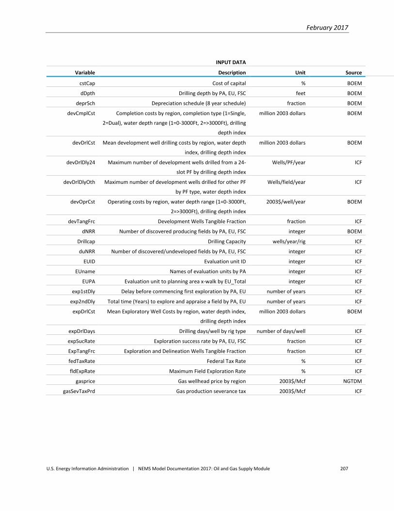
February 2017


INPUT DATA

Variable Description Unit Source

cstCap Cost of capital % BOEM

dDpth Drilling depth by PA, EU, FSC feet BOEM

deprSch Depreciation schedule (8 year schedule) fraction BOEM

devCmplCst Completion costs by region, completion type (1=Single,

2=Dual), water depth range (1=0-3000Ft, 2=>3000Ft), drilling

depth index

million 2003 dollars BOEM

devDrlCst Mean development well drilling costs by region, water depth

index, drilling depth index


devDrlDly24 Maximum number of development wells drilled from a 24-

slot PF by drilling depth index

Wells/PF/year ICF

devDrlDlyOth Maximum number of development wells drilled for other PF

by PF type, water depth index

Wells/field/year ICF

devOprCst Operating costs by region, water depth range (1=0-3000Ft,

2=>3000Ft), drilling depth index

2003$/well/year BOEM

devTangFrc Development Wells Tangible Fraction fraction ICF

dNRR Number of discovered producing fields by PA, EU, FSC integer BOEM

Drillcap Drilling Capacity wells/year/rig ICF

duNRR Number of discovered/undeveloped fields by PA, EU, FSC integer ICF

EUID Evaluation unit ID integer ICF

EUname Names of evaluation units by PA integer ICF

EUPA Evaluation unit to planning area x-walk by EU_Total integer ICF

exp1stDly Delay before commencing first exploration by PA, EU number of years ICF

exp2ndDly Total time (Years) to explore and appraise a field by PA, EU number of years ICF

expDrlCst Mean Exploratory Well Costs by region, water depth index,

drilling depth index


expDrlDays Drilling days/well by rig type number of days/well ICF

expSucRate Exploration success rate by PA, EU, FSC fraction ICF

ExpTangFrc Exploration and Delineation Wells Tangible Fraction fraction ICF

fedTaxRate Federal Tax Rate % ICF

fldExpRate Maximum Field Exploration Rate % ICF

gasprice Gas wellhead price by region 2003$/Mcf NGTDM

gasSevTaxPrd Gas production severance tax 2003$/Mcf ICF

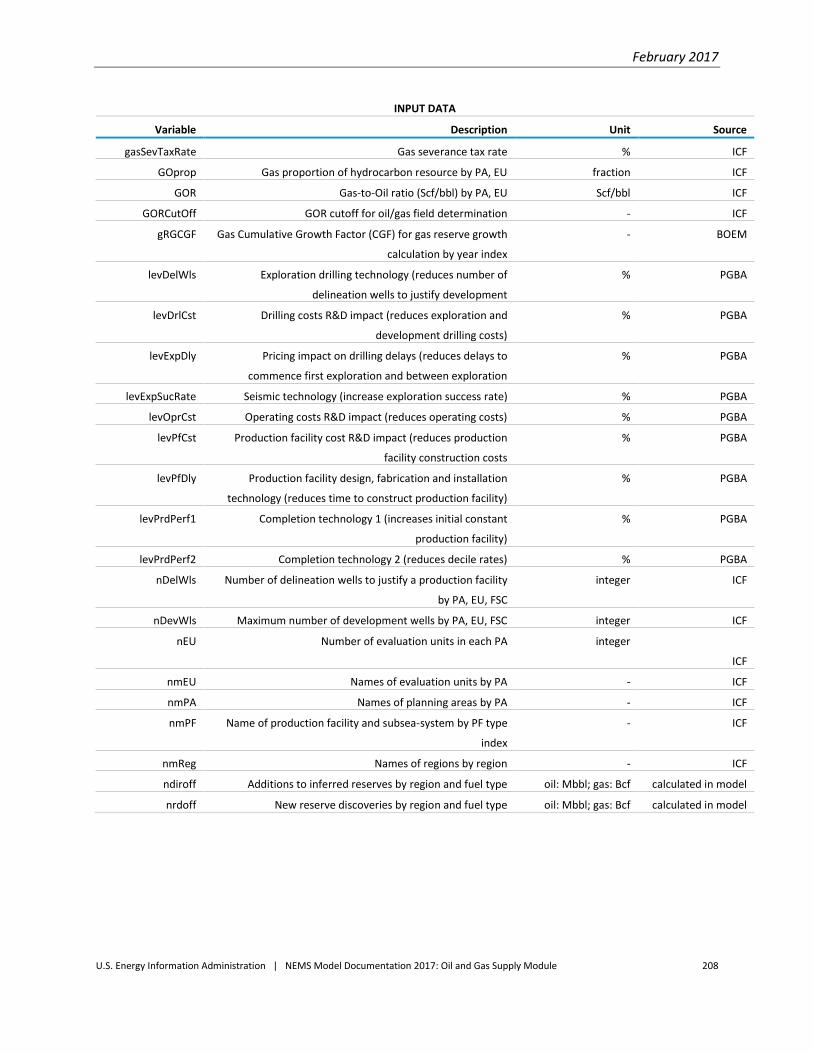
February 2017


INPUT DATA


gasSevTaxRate Gas severance tax rate % ICF

GOprop Gas proportion of hydrocarbon resource by PA, EU fraction ICF

GOR Gas-to-Oil ratio (Scf/bbl) by PA, EU Scf/bbl ICF

GORCutOff GOR cutoff for oil/gas field determination - ICF

gRGCGF Gas Cumulative Growth Factor (CGF) for gas reserve growth

calculation by year index

- BOEM

levDelWls Exploration drilling technology (reduces number of

delineation wells to justify development

% PGBA

levDrlCst Drilling costs R&D impact (reduces exploration and

development drilling costs)

% PGBA

levExpDly Pricing impact on drilling delays (reduces delays to

commence first exploration and between exploration

% PGBA

levExpSucRate Seismic technology (increase exploration success rate) % PGBA

levOprCst Operating costs R&D impact (reduces operating costs) % PGBA

levPfCst Production facility cost R&D impact (reduces production

facility construction costs

% PGBA

levPfDly Production facility design, fabrication and installation

technology (reduces time to construct production facility)

% PGBA

levPrdPerf1 Completion technology 1 (increases initial constant

production facility)

% PGBA

levPrdPerf2 Completion technology 2 (reduces decile rates) % PGBA

nDelWls Number of delineation wells to justify a production facility

by PA, EU, FSC

integer ICF

nDevWls Maximum number of development wells by PA, EU, FSC integer ICF

nEU Number of evaluation units in each PA integer

ICF

nmEU Names of evaluation units by PA - ICF

nmPA Names of planning areas by PA - ICF

nmPF Name of production facility and subsea-system by PF type

index

- ICF

nmReg Names of regions by region - ICF

ndiroff Additions to inferred reserves by region and fuel type oil: Mbbl; gas: Bcf calculated in model

nrdoff New reserve discoveries by region and fuel type oil: Mbbl; gas: Bcf calculated in model

February 2017


INPUT DATA


nRigs Number of rigs by rig type integer ICF

nRigWlsCap Number of well drilling capacity (Wells/Rig) wells/rig ICF

nRigWlsUtl Number of wells drilled (Wells/Rig) wells/rig ICF

nSlt Number of slots by # of slots index integer ICF

oilPrcCstTbl Oil price for cost tables 2003$/bbl ICF

oilprice Oil wellhead price by region 2003$/bbl LFMM

oilSevTaxPrd Oil production severance tax 2003$/bbl ICF

oilSevTaxRate Oil severance tax rate % ICF

oRGCGF Oil Cumulative Growth Factor (CGF) for oil reserve growth

calculation by year index

fraction BOEM

paid Planning area ID integer ICF

PAname Names of planning areas by PA - ICF

pfBldDly1 Delay for production facility design, fabrication, and

installation (by water depth index, PF type index, # of slots

index (0 for non-platform)

number of years ICF

pfBldDly2 Delay between production facility construction by water

depth index

number of years ICF

pfCst Mean Production Facility Costs in by region, PF type, water

depth index, # of slots index (0 for non-platform)

million 2003$ BOEM

pfCstFrc Production facility cost fraction matrix by year index, year

index

fraction ICF

pfMaxNFld Maximum number of fields in a project by project option integer ICF

pfMaxNWls Maximum number of wells sharing a flowline by project

option

integer ICF

pfMinNFld Minimum number of fields in a project by project option integer ICF

pfOptFlg Production facility option flag by water depth range index,

FSC

- ICF

pfTangFrc Production Facility Tangible Fraction fraction ICF

pfTypFlg Production facility type flag by water depth range index, PF

type index

- ICF

platform Flag for platform production facility - ICF

prd_DEPTH Producing fields - Total drilling depth feet BOEM

prd_EU Producing fields - Evaluation unit name - ICF

prd_FLAG Producing fields - Production decline flag - ICF

February 2017


INPUT DATA


prd_FN Producing fields - Field name - BOEM

prd_ID Producing fields - BOEM field ID - BOEM

prd_OG Producing fields - Fuel type - BOEM

prd_YRDISC Producing fields - Year of discovery year BOEM

prdDGasDecRatei Initial gas decline rate by PA, EU, FSC range index fraction/year ICF

prdDGasHyp Gas hyperbolic decline coefficient by PA, EU, FSC range

index

fraction ICF

prdDOilDecRatei Initial oil decline rate by PA, EU, fraction/year ICF

prdDOilHyp Oil hyperbolic decline coefficient by PA, EU, FSC range

index

fraction ICF

prdDYrPeakGas Years at peak production for gas by PA, EU, FSC, range

index

number of years ICF

prdDYrPeakOil Years at peak production for oil by PA, EU, FSC, range index number of years ICF

prdDYrRampUpGas Years to ramp up for gas production by PA, EU, FSC range

index

number of years ICF

prdDYrRampUpOil Years to ramp up for oil production by PA, EU, FSC range

index

number of years ICF

prdGasDecRatei Initial gas decline rate by PA, EU fraction/year ICF

prdGasFrc Fraction of gas produced before decline by PA, EU fraction ICF

prdGasHyp Gas hyperbolic decline coefficient by PA, EU fraction ICF

prdGasRatei Initial gas production (Mcf/Day/Well) by PA, EU Mcf/day/well ICF

PR Expected production to reserves ratio by fuel type fraction PGBA

prdoff Expected production by fuel type oil:Mbbl; gas: Bcf calculated in model

prdOilDecRatei Initial oil decline rate by PA, EU fraction/year ICF

prdOilFrc Fraction of oil produced before decline by PA, EU fraction ICF

prdOilHyp Oil hyperbolic decline coefficient by PA, EU fraction ICF

prdOilRatei Initial oil production (Bbl/Day/Well) by PA, EU bbl/day/well ICF

prod Producing fields - annual production by fuel type oil:Mbbl; gas:MMcf BOEM

prod_asg AD gas production Bcf calculated in model

revoff Extensions, revisions, and adjustments by fuel type oil:Mbbl; gas:Bcf

rigBldRatMax Maximum Rig Build Rate by rig type % ICF

rigIncrMin Minimum Rig Increment by rig type integer ICF

RigUtil Number of wells drilled wells/rig ICF

rigUtilTarget Target Rig Utilization by rig type % ICF

royRateD Royalty rate for discovered fields by PA, EU, FSC fraction BOEM

royRateU Royalty rate for undiscovered fields by PA, EU, FSC fraction BOEM

February 2017


INPUT DATA


stTaxRate Federal Tax Rate by PA, EU % ICF

trnFlowLineLen Flowline length by PA, EU Miles/prospect ICF

trnPpDiam Oil pipeline diameter by PA, EU inches ICF

trnPplnCst Pipeline cost by region, pipe diameter index, water depth

index

million 2003$/mile BOEM

trnTrfGas Gas pipeline tariff ($/Mcf) by PA, EU 2003$/bbl ICF

trnTrfOil Oil pipeline tariff ($/bbl) by PA, EU 2003$/bbl ICF

uNRR Number of undiscovered fields by PA, EU, FSC integer calculated in model

vMax Maximum MMBOE of FSC MMBOE BOEM

vMean Geometric mean MMBOE of FSC MMBOE BOEM

vMin Minimum MMBOE of FSC MMBOE BOEM

wDpth Water depth by PA, EU, FSC feet BOEM

yrAvl Year lease available by PA, EU year ICF

yrCstTbl Year of cost tables year ICF

Sources: BOEM = Bureau of Ocean Energy Management (formerly the Minerals Management Service); ICF = ICF Consulting; PGBA =

EIA, Office of Petroleum, Natural Gas, and Biofuels Analysis.

February 2017


4. Alaska Oil and Gas Supply Submodule

This section describes the structure for the Alaska Oil and Gas Supply Submodule (AOGSS). The AOGSS is

designed to project field-specific oil production from the Onshore North Slope, Offshore North Slope,

and Other Alaska areas (primarily the Cook Inlet area). The North Slope region encompasses the

National Petroleum Reserve Alaska in the west, the State Lands in the middle, and the Arctic National

Wildlife Refuge area in the east. This section provides an overview of the basic modeling approach,

including a discussion of the discounted cash flow (DCF) method.

Alaska natural gas production is not projected by the AOGSS, but by the Natural Gas Transmission and

Distribution Module (NGTDM). The NGTDM projects Alaska gas consumption and whether an Alaska gas

pipeline is projected to be built to carry Alaska North Slope gas into Canada and U.S. gas markets. As of

January 1, 2012, Alaska was estimated to have 10 trillion cubic feet of proved reserves plus 271 trillion

cubic feet of unproved resources, excluding the Arctic National Wildlife Refuge undiscovered gas

resources. Over the long term, Alaska natural gas production is determined and constrained by local

consumption and by the capacity of a gas pipeline that might be built to serve Canada and U.S. lower 48

markets. The proved and inferred gas resources alone, plus known but undeveloped resources, are

sufficient to satisfy at least 20 years of Alaska gas consumption and gas pipeline throughput. Moreover,

large deposits of natural gas have been discovered along the North Slope (e.g., Point Thomson) but

remain undeveloped due to a lack of access to gas consumption markets. Because Alaska natural gas

production is best determined by projecting Alaska gas consumption and whether a gas pipeline is put

into operation, the AOGSS does not attempt to project new gas field discoveries and their development

or the declining production from existing fields.

AOGSS overview The AOGSS solely focuses on projecting the exploration and development of undiscovered oil resources,

primarily with respect to the oil resources expected to be found onshore and offshore in North Alaska.

The AOGSS is divided into three components: new field discoveries, development projects, and

producing fields (Figure 4-1). Transportation costs are used in conjunction with the crude oil price to

Southern California refineries to calculate an estimated wellhead (netback) oil price. A discounted cash

flow (DCF) calculation is used to determine the economic viability of Alaskan drilling and production

activities. Oil field investment decisions are modeled on the basis of discrete projects. The exploration,

discovery, and development of new oil fields depend on the expected exploration success rate and new

field profitability. Production is determined on the basis of assumed drilling schedules and production

profiles for new fields and developmental projects, along with historical production patterns and

announced plans for currently producing fields.

February 2017


Figure 4-1. Flowchart of the Alaska Oil and Gas Supply Submodule

February 2017


As of January 1, 2012, Alaska onshore and offshore technically recoverable oil resources equal 4 billion

barrels of proved reserves plus 34 billion barrels of unproved resources.

Calculation of costs

Costs differ within the model for successful wells and dry holes. Costs are categorized functionally within

the model as

Drilling costs

Lease equipment costs

Operating costs (including production facilities and general and administrative costs)

All costs in the model incorporate the estimated impact of environmental compliance. Environmental

regulations that preclude a supply activity outright are reflected in other adjustments to the model. For

example, environmental regulations that preclude drilling in certain locations within a region are

modeled by reducing the recoverable resource estimates for that region.

Each cost function includes a variable that reflects the cost savings associated with technological

improvements. As a result of technological improvements, average costs decline in real terms relative

to what they would otherwise be. The degree of technological improvement is a user-specified option in

the model. The equations used to estimate costs are similar to those used for the lower 48 but include

cost elements that are specific to Alaska. For example, lease equipment includes gravel pads and ice

roads.

Drilling costs

Drilling costs are the expenditures incurred for drilling both successful wells and dry holes, and for

equipping successful wells through the "Christmas tree," the valves and fittings assembled at the top of

a well to control the fluid flow. Elements included in drilling costs are labor, material, supplies and direct

overhead for site preparation, road building, erecting and dismantling derricks and drilling rigs, drilling,

running and cementing casing, machinery, tool changes, and rentals. Drilling costs for exploratory wells

include costs of support equipment such as ice pads. Lease equipment required for production is

included as a separate cost calculation and covers equipment installed on the lease downstream from

the Christmas tree.

The average cost of drilling a well in any field located within region r in year t is given by:

)T*(t*1)TECH - (1 * DRILLCOST = DRILLCOST bTk,r,i,tk,r,i, b (4-18)

where

i = well class (exploratory=1, developmental=2)

r = region (Offshore North Slope = 1, Onshore North Slope = 2, Cook Inlet = 3)

k = fuel type (oil=1, gas=2 - but not used)

February 2017


t = forecast year

DRILLCOST = drilling costs

Tb = base year of the forecast

TECH1 = annual decline in drilling costs due to improved technology.

The above function specifies that drilling costs decline at the annual rate specified by TECH1. Drilling

costs are not modeled as a function of the drilling rig activity level as they are in the Onshore Lower 48

methodology. Drilling rigs and equipment are designed specifically for the harsh Arctic weather

conditions. Once drilling rigs are moved up to Alaska and reconfigured for Arctic conditions, they

typically remain in Alaska. Company drilling programs in Alaska are planned to operate at a relatively

constant level of activity because of the limited number of drilling rigs and equipment available for use.

Most Alaska oil rig activity pertains to drilling in-fill wells intended to slow the rate of production decline

in the largest Alaska oil fields.

Alaska onshore and offshore drilling and completion costs were updated in 2010 based on the American Petroleum Institute’s (API) 2007 Joint Association Survey on Drilling Costs, dated December 2008. Based on these API drilling and completion costs and earlier work performed by Advanced Resources International, Inc. in 2002, the following oil well drilling and completion costs were incorporated into the AOGSS database (Table 4.1).

Table 4-1. AOGSS oil well drilling and completion costs by location and category

New Field Wildcat Wells New Exploration Wells Developmental Wells

In millions of 2011 dollars

Offshore North Slope 220 110 105

Onshore North Slope 160 80 60

South Alaska 78 63 39

In millions of 1990 dollars

Offshore North Slope 140 70 67

Onshore North Slope 102 51 39

South Alaska 50 40 25

Table 1 provides both 1990 and 2011 well drilling and completion cost data because the former are used

within the context of calculating AOGSS discounted cash flows, while the latter are comparable to the

current price environment.

Lease equipment costs

Lease equipment costs include the cost of all equipment extending beyond the Christmas tree, directly

used to obtain production from a developed lease. Costs include: producing equipment, the gathering

system, processing equipment (e.g., oil/gas/water separation), and production-related infrastructure

such as gravel pads. Producing equipment costs include tubing, pumping equipment. Gathering system

February 2017


costs consist of flowlines and manifolds. The lease equipment cost estimate for a new oil well is given

by

EQUIPr,k,t = EQUIPr,k,Tb∗ (1 − TECH2)t−Tb (4-19)

where


k = fuel type (oil = 1, gas = 2 – not used)

t = forecast year

EQUIP = lease equipment costs


TECH2 = annual decline in lease equipment costs due to improved technology.

Operating costs

EIA operating cost data, which are reported on a per-well basis for each region, include three main

categories of costs: normal daily operations, surface maintenance, and subsurface maintenance.

Normal daily operations are further broken down into supervision and overhead, labor, chemicals, fuel,

water, and supplies. Surface maintenance accounts for all labor and materials necessary to keep the

service equipment functioning efficiently and safely. Costs of stationary facilities, such as roads, also are

included. Subsurface maintenance refers to the repair and services required to keep the downhole

equipment functioning efficiently.

The estimated operating cost curve is:

OPCOSTr,k,t = OPCOSTr,k,Tb∗ (1 − TECH2)t−Tb (4-20)

where


k = fuel type (oil = 1, gas = 2 – not used)

t = forecast year

OPCOST = operating cost


TECH3 = annual decline in operating costs due to improved technology.

February 2017


Drilling costs, lease equipment costs, and operating costs are integral components of the following

discounted cash flow analysis. These costs are assumed to be uniform across all fields within each of the

three Alaskan regions.

Treatment of costs in the model for income tax purposes

All costs are treated for income tax purposes as either expensed or capitalized. The tax treatment in the

DCF reflects the applicable provisions for oil producers. The DCF assumptions are consistent with

standard accounting methods and with assumptions used in similar modeling efforts. The following

assumptions, reflecting current tax law, are used in the calculation of costs.

All dry-hole costs are expensed.

A portion of drilling costs for successful wells is expensed. The specific split between expensing

and amortization is based on the tax code.

Operating costs are expensed.

All remaining successful field development costs are capitalized.

The depletion allowance for tax purposes is not included in the model, because the current

regulatory limitations for invoking this tax advantage are so restrictive as to be insignificant in

the aggregate for future drilling decisions.

Successful versus dry-hole cost estimates are based on historical success rates of successful

versus dry-hole footage.

Lease equipment for existing wells is in place before the first forecast year of the model.

Discounted cash flow analysis A discounted cash flow (DCF) calculation is used to determine the profitability of oil projects.12 A

positive DCF is necessary to initiate the development of a discovered oil field. With all else being equal,

large oil fields are more profitable to develop than small and mid-size fields. In Alaska, where

developing new oil fields is quite expensive, particularly in the Arctic, the profitable development of

small and mid-size oil fields is generally contingent on the pre-existence of infrastructure that was paid

for by the development of a nearby large field. Consequently, AOGSS assumes that the largest oil fields

will be developed first, followed by the development of ever-smaller oil fields. Whether these oil fields

are developed, regardless of their size, is projected on the basis of the profitability index, which is

measured as the ratio of the expected discounted cash flow to expected capital costs for a potential

project.

A key variable in the DCF calculation is the oil transportation cost to southern California refineries.

Transportation costs for Alaskan oil include both pipeline and tanker shipment costs. The oil

transportation cost directly affects the expected revenues from the production of a field as follows:13

REV Q *(MP TRANS )f,t f,t t t (4-21)

12 See Appendix 3.A at the end of this chapter for a detailed discussion of the DCF methodology. 13 This formulation assumes oil production only. It can be easily expanded to incorporate the sale of natural gas.

February 2017


where

f = field

t = year

REV = expected revenues

Q = expected production volumes

MP = market price in the lower 48 states

TRANS = transportation cost.

The expected discounted cash flow associated with a potential oil project in field f at time t is given by

(4-22)

where

PVREV = present value of expected revenues

PVROY = present value of expected royalty payments

PVDRILLCOST = present value of all exploratory and developmental drilling expenditures

PVEQUIP = present value of expected lease equipment costs

TRANSCAP = cost of incremental transportation capacity

PVOPCOST = present value of operating costs

PVPRODTAX = present value of expected production taxes (ad valorem and severance taxes)

PVSIT = present value of expected state corporate income taxes

PVFIT = present value of expected federal corporate income taxes

The expected capital costs for the proposed field f located in region r are

COST (PVEXPCOST PVDEVCOST PVEQUIP TRANSCAP)f,t f,t (4-23)

where

PVEXPCOST = present value exploratory drilling costs

PVDEVCOST = present value developmental drilling costs

PVEQUIP = present value lease equipment costs

TRANSCAP = cost of incremental transportation capacity

The profitability indicator from developing the proposed field is therefore

PROFDCF

COSTf,t

f,t

f,t

. (4-24)

DCF (PVREV PVROY PVDRILLCOST PVEQUIP TRANSCAP

PVOPCOST PVPRODTAX PVSIT PVFIT)

f,t

f,t

February 2017


The model assumes that the field with the highest positive PROF in time t is eligible for exploratory

drilling in the same year. The profitability indices for Alaska also are passed to the basic framework

module of the OGSM.

New field discovery Development of estimated recoverable resources, which are expected to be in currently undiscovered

fields, depends on the schedule for the conversion of resources from unproved to reserve status. The

conversion of resources into field reserves requires both a successful new field wildcat well and a

positive discounted cash flow of the costs relative to the revenues. The discovery procedure can be

determined endogenously, based on exogenously determined data. The procedure requires the

following exogenously determined data:

new field wildcat success rate

any restrictions on the timing of drilling

the distribution of technically recoverable field sizes within each region

The endogenous procedure generates:

the new field wildcat wells drilled in any year

the set of individual fields to be discovered, specified with respect to size and location (relative

to the three Alaska regions, i.e., offshore North Slope, onshore North Slope, and South-Central

Alaska)

an order for the discovery sequence

a schedule for the discovery sequence

The new field discovery procedure relies on the U.S. Geological Survey (USGS) and Bureau of Ocean

Energy Management (BOEM) respective estimates of onshore and offshore technically recoverable oil

resources as translated into the expected field size distribution of undiscovered fields. These onshore

and offshore field size distributions are used to determine the field size and order of discovery in the

AOGSS exploration and discovery process. Thus, the AOGSS oil field discovery process is consistent with

the expected geology with respect to expected aggregate resource base and the relative frequency of

field sizes.

AOGSS assumes that the largest fields in a region are found first, followed by successively smaller fields.

This assumption is based on the following observations: 1) the largest-volume fields typically encompass

the greatest areal extent, thereby raising the probability of finding a large field relative to finding a

smaller field, 2) seismic technology is sophisticated enough to be able to determine the location of the

largest geologic structures that might possibly hold oil, 3) producers have a financial incentive to

develop the largest fields first both because of their higher inherent rate of return and because the

largest fields can pay for the development of expensive infrastructure that affords the opportunity to

develop the smaller fields using that same infrastructure, and 4) historically, North Slope and Cook Inlet

field development has generally progressed from largest field to smallest field.

February 2017


Onshore and offshore North Slope new field wildcat drilling activity is a function of West Texas

Intermediate crude oil prices from 1977 through 2008, expressed in 2008 dollars. The new field wildcat

exploration function was statistically estimated based on West Texas Intermediate crude oil prices from

1977 through 2008 and on exploration well drilling data obtained from the Alaska Oil and Gas

Conservation Commission (AOGCC) data files for the same period.14 The North Slope wildcat exploration

drilling parameters were estimated using ordinary least squares methodology.

77.3)WOP_IT13856.0(NFW_NAK tt (4-8)

where

t = year

NAK_NFWt = North Slope Alaska field wildcat exploration wells

IT_WOPt = World oil price in 2008 dollars

The summary statistics for the statistical estimation are as follows:

Dependent variable: NSEXPLORE

Current sample: 1 to 32

Number of observations: 32

Mean of dep. var. = 9.81250 LM het. test = .064580 [.799]

Std. dev. of dep. var. = 4.41725 Durbin-Watson = 2.04186 [<.594]

Sum of squared residuals = 347.747 Jarque-Bera test = .319848 [.852]

Variance of residuals = 11.5916 Ramsey's RESET2 = .637229E-04 [.994]

Std. error of regression = 3.40464 F (zero slopes) = 22.1824 [.000]

R-squared = .425094 Schwarz B.I.C. = 87.0436

Adjusted R-squared = .405930 Log likelihood = -83.5778

Estimated Standard

Variable Coefficient Error t-statistic P-value

C 3.77029 1.41706 2.66065 [.012]

WTIPRICE .138559 .029419 4.70982 [.000]

Because very few offshore North Slope wells have been drilled since 1977, within AOGSS, the total

number of exploration wells drilled on the North Slope is shared between the onshore and offshore

regions, with the wells being predominantly drilled onshore in the early years of the projections with

progressively more wells drilled offshore, such that after 20 years, 50% of the exploration wells are

drilled onshore and 50% are drilled offshore.

Based on the AOGCC data for 1977 through 2008, the drilling of South-Central Alaska new field wildcat

exploration wells was statistically unrelated to oil prices. On average, three exploration wells per year

14 A number of alternative functional formulations were tested (e.g., using Alaska crude oil prices, lagged oil prices, etc.), yet

none of the alternative formations resulted in statistically more significant relationships.

February 2017


were drilled in South-Central Alaska over the 1977 through 2008 timeframe, regardless of prevailing oil

prices. This result probably stems from the fact that most of the South-Central Alaska drilling activity is

focused on natural gas rather than oil, and that natural gas prices are determined by the Regulatory

Commission of Alaska rather than being “market driven.” Consequently, AOGSS specifies that three

exploration wells are drilled each year.

The execution of the above procedure can be modified to reflect restrictions on the timing of discovery

for particular fields. Restrictions may be warranted for enhancements such as delays necessary for

technological development needed prior to the recovery of relatively small accumulations or heavy oil

deposits. State and federal lease sale schedules could also restrict the earliest possible date for

beginning the development of certain fields. This refinement is implemented by declaring a start date

for possible exploration. For example, AOGSS specifies that if federal leasing in the Arctic National

Wildlife Refuge were permitted in 2011, then the earliest possible date at which an ANWR field could

begin oil production would be in 2021.15 Another example is the wide-scale development of the West

Sak field that is being delayed until a technology can be developed that will enable the heavy, viscous

crude oil of that field to be economically extracted.

Development projects Development projects are those projects in which a successful new field wildcat has been drilled. As

with the new field discovery process, the DCF calculation plays an important role in the timing of

development and exploration of these multi-year projects.

Each model year, the DCF is calculated for each potential development project. Initially, the model

assumes a drilling schedule determined by the user or by some set of specified rules. However, if the

DCF for a given project is negative, then development of this project is suspended in the year in which

the negative DCF occurs. The DCF for each project is evaluated in subsequent years for a positive value.

The model assumes that development would resume when a positive DCF value is calculated.

Production from developing projects follows the generalized production profile developed for and

described in previous work conducted by DOE staff. 16 The specific assumptions used in this work are as

follows:

a 2- to 4-year build-up period from initial production to the peak production rate

the peak production rate is sustained for 3 to 8 years

after peak production, the production rate declines by 12% to 15% per year

The production algorithm build-up and peak-rate period are based on the expected size of the

undiscovered field, with larger fields having longer build-up and peak-rate periods than the smaller

fields. The field production decline rates are also determined by the field size.

15 The earliest ANWR field is assumed to go into production 10 years after the first projection year. 16 Potential Oil Production from the Coastal Plain of the Arctic National Wildlife Refuge: Updated Assessment, EIA (May 2000)

and Alaska Oil and Gas - Energy Wealth of Vanishing Opportunity?, DOE/ID/0570-H1 (January 1991).

February 2017


The pace of development and the ultimate number of wells drilled for a particular field is based on the

historical field-level profile adjusted for field size and other characteristics of the field (e.g. API gravity).

Producing fields Oil production from fields producing as of the initial projection year (e.g., Prudhoe Bay, Kuparuk,

Lisburne, Endicott, and Milne Point) is based on historical production patterns, remaining estimated

recovery, and announced development plans. The production decline rates of these fields are

periodically recalibrated based on recent field-specific production rates.

Natural gas production from the North Slope for sale to end-use markets depends on the construction of

a pipeline to transport natural gas to lower 48 markets.17 North Slope natural gas production is

determined by the carrying capacity of a natural gas pipeline to the lower 48.18 The Prudhoe Bay Field

is the largest known deposit of North Slope gas (24.5 Tcf)19 and currently all of the gas produced from

this field is re-injected to maximize oil production. Total known North Slope gas resources equal 35.420

Tcf. Furthermore, the undiscovered onshore central North Slope and NPRA technically recoverable

natural gas resource base are respectively estimated to be 33.3 Tcf21 and 52.8 Tcf.22 Collectively, these

North Slope natural gas reserves and resources equal 121.5 Tcf, which would satisfy the 1.64 Tcf per

year gas requirements of an Alaska gas pipeline for almost 75 years, well after the end of the Annual

Energy Outlook projections. Consequently, North Slope natural gas resources, both discovered and

undiscovered, are more than ample to supply natural gas to an Alaska gas pipeline during the Annual

Energy Outlook projection period.

During the development of the Annual Energy Outlook 2012, a new algorithm was added with respect to

North Slope oil production. The new algorithm was predicated on the notion that the Alyeska Oil

Pipeline (also known as the Trans Alaska Pipeline System or TAPS) might be unable to operate below

350,000 barrels per day, if North Slope wellhead oil revenues were insufficient to pay for the pipeline

upgrades necessary to keep the pipeline operating at low flow rates.

In August 2008, Alyeska initiated the Low Flow Impact Study (Study) that was released on June 15,

2011.23 The Alyeska Study identified the following potential problems that might occur as TAPS

throughput declines from the current production levels:

17 Initial natural gas production from the North Slope for Lower 48 markets is affected by a delay reflecting a reasonable period

for construction. Details of how this decision is made in NEMS are included in the Natural Gas Transmission and Distribution

Module documentation. 18 The determination of whether an Alaska gas pipeline is economically feasible is calculated within the Natural Gas

Transmission and Distribution Model. 19 Alaska Oil and Gas Report 2009, Alaska Department of Natural Resources, Division of Oil and Gas, Table I.I, page 8. 20 Ibid. 21 U.S. Geological Survey, Oil and Gas Assessment of Central North Slope, Alaska, 2005, Fact Sheet 2005-3043, April 2005, page 2

table – mean estimate total. 22 U.S. Geological Survey, 2010 Updated Assessment of Undiscovered Oil and Gas Resources of the National Petroleum Reserve

in Alaska (NPRA), Fact Sheet 2010-3102, October 2010, Table 1 – mean estimate total, page 4. 23 Alyeska Pipeline Service Company, Low Flow Impact Study, Final Report, June 15, 2011, Anchorage, Alaska, at

http://www.alyeska-pipe.com/Inthenews/LowFlow/LoFIS_Summary_Report_P6%2027_FullReport.pdf.

http://www.alyeska-pipe.com/Inthenews/LowFlow/LoFIS_Summary_Report_P6%2027_FullReport.pdf

February 2017


potential water dropout from the crude oil, which could cause pipeline corrosion

potential ice formation in the pipe if the oil temperature were to drop below freezing

potential wax precipitation and deposition

potential soil heaving

other potential operational issues at low flow rates include: sludge drop-out, reduced ability to

remove wax, reduction in pipeline leak detection efficiency, pipeline shutdown and restart, and

the running of pipeline pigs that both clean and check pipeline integrity

Although the onset of TAPS low flow problems could begin at around 550,000 barrels per day, absent

any mitigation, the severity of the TAPS operational problems is expected to increase as throughput

declines. As the types and severity of problems multiplies, the investment required to mitigate those

problems is expected to increase significantly. Because of the many and diverse operational problems

expected to occur below 350,000 barrels per day of throughput, considerable investment might be

required to keep the pipeline operational below this threshold.

Starting with AEO2012, it was assumed that the North Slope oil fields would be shut down, plugged, and

abandoned if the following two conditions were simultaneously satisfied: 1) TAPS throughput would

have to be at or below 350,000 barrels per day and 2) total North Slope oil production revenues would

have to be at or below $5.0 billion per year. In the year in which these two conditions were

simultaneously satisfied, it was assumed that 1) TAPS would be decommissioned and dismantled and 2)

North Slope oil exploration and production activities would cease. A more detailed discussion regarding

these assumptions and their rationale is found in the AEO2012 report analysis entitled "Potential impact

of minimum pipeline throughput constraints on Alaska North Slope oil production" on pages 52 to 56 in

the PDF version. As pointed out in the AEO2012 analysis, these two conditions are only satisfied in the

Low Oil Price Case in 2026, when North Slope oil production and TAPS are shut down.

The determination of whether Alaska North slope oil production is shut down during an Annual Energy

Outlook projection is a two-step process. The first step is the determination of total onshore and

offshore North Slope oil revenues. Total North Slope oil revenues equal onshore and offshore oil

production multiplied by the result of a subtraction of the world oil price minus the transportation cost

of shipping oil through TAPS and by tanker to West Coast refineries. The second step simultaneously

compares whether total onshore and offshore oil production falls below the 350,000 barrels per day

minimum TAPS throughput level and whether total onshore and offshore North Slope oil wellhead

production revenues fall below the $5 billion per year minimum revenue threshold. If both conditions

are simultaneously satisfied in any specific year, then TAPSFLAG variable is set to zero and onshore and

offshore oil production levels are set to zero in that year and future years, thereby precluding future

North Slope oil production.

The total transportation cost of shipping oil from the North Slope depends upon whether the oil is

produced offshore or onshore, with the offshore oil transportation cost being higher than the onshore

transportation cost. Both the onshore and offshore transportation costs per barrel of oil are held

constant throughout the projections, based on current TAPS and marine tanker transportation costs.

However, the per-barrel TAPS transportation cost would be expected to increase over time both due to

February 2017


declining TAPS throughput and due to higher total TAPS operation and maintenance costs as the

pipeline ages and as the TAPS operator increasingly invests more money to mitigate the problems

created by lower flow rates. Consequently, TAPS and North Slope oil production could be shut down

earlier than that projected in the Low Oil Price Case.

February 2017


Appendix 4.A. Alaskan Data Inventory

Variable Name

Description

Unit

Classification

Source Code Text

ANGTSMAX -- ANGTS maximum flow Bcf/d Alaska NPC

ANGTSPRC -- Minimum economic price for

ANGTS start up

1987$/Mcf Alaska NPC

ANGTSRES -- ANGTS reserves Bcf Alaska NPC

ANGTSYR -- Earliest start year for ANGTS

flow

Year NA NPC

DECLPRO -- Alaska decline rates for

currently producing fields

Fraction Field OPNGBA

DEV_AK -- Alaska drilling schedule for

developmental wells

Wells per

year

3 Alaska regions;

Fuel (oil, gas)

OPNGBA

DRILLAK DRILL Alaska drilling cost (not

including new field wildcats)

1990$/well Class (exploratory,

developmental);

3 Alaska regions;

Fuel (oil, gas)

OPNGBA

DRLNFWAK -- Alaska drilling cost of a new

field wildcat

1990$/well 3 Alaska regions;

Fuel (oil, gas)

OPNGBA

DRYAK DRY Alaska dry hole cost 1990$/hole Class (exploratory,

developmental);

3 Alaska regions;

Fuel (oil, gas)

OPNGBA

EQUIPAK EQUIP Alaska lease equipment cost 1990$/well Class (exploratory,

developmental); 3

Alaska regions; Fuel

(oil, gas)

USGS

EXP_AK -- Alaska drilling schedule for

other exploratory wells

wells per

year

3 Alaska regions OPNGBA

FACILAK -- Alaska facility cost (oil field) 1990$/bls Field size class USGS

FSZCOAK -- Alaska oil field size

distributions

MMbbl 3 Alaska regions USGS

FSZNGAK -- Alaska gas field size

distributions

Bcf 3 Alaska regions USGS

HISTPRDCO -- Alaska historical crude oil

production

Mbbl/d Field AOGCC

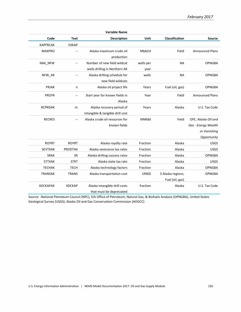
February 2017


Variable Name

Code Text Description Unit Classification Source

KAPFRCAK EXKAP

MAXPRO -- Alaska maximum crude oil

production

Mbbl/d Field Announced Plans

NAK_NFW -- Number of new field wildcat

wells drilling in Northern AK

wells per

year

NA OPNGBA

NFW_AK -- Alaska drilling schedule for

new field wildcats

wells NA OPNGBA

PRJAK n Alaska oil project life Years Fuel (oil, gas) OPNGBA

PROYR -- Start year for known fields in

Alaska

Year Field Announced Plans

RCPRDAK m Alaska recovery period of

intangible & tangible drill cost

Years Alaska U.S. Tax Code

RECRES -- Alaska crude oil resources for

known fields

MMbbl Field OFE, Alaska Oil and

Gas - Energy Wealth

or Vanishing

Opportunity

ROYRT ROYRT Alaska royalty rate Fraction Alaska USGS

SEVTXAK PRODTAX Alaska severance tax rates Fraction Alaska USGS

SRAK SR Alaska drilling success rates Fraction Alaska OPNGBA

STTXAK STRT Alaska state tax rate Fraction Alaska USGS

TECHAK TECH Alaska technology factors Fraction Alaska OPNGBA

TRANSAK TRANS Alaska transportation cost 1990$ 3 Alaska regions;

Fuel (oil, gas)

OPNGBA

XDCKAPAK XDCKAP Alaska intangible drill costs

that must be depreciated

fraction Alaska U.S. Tax Code

Source: National Petroleum Council (NPC), EIA Office of Petroleum, Natural Gas, & Biofuels Analysis (OPNGBA), United States

Geological Survey (USGS), Alaska Oil and Gas Conservation Commission (AOGCC)

February 2017


5. Oil Shale Supply Submodule

Oil shale rock contains a hydrocarbon known as kerogen,24 which can be processed into a synthetic

crude oil (syncrude) by heating the rock. During the 1970s and early 1980s, petroleum companies

conducted extensive research, often with the assistance of public funding, into the mining of oil shale

rock and the chemical conversion of the kerogen into syncrude. The technologies and processes

developed during that period are well-understood and well-documented with extensive technical data

on demonstration plant costs and operational parameters, which were published in the professional

literature. The Oil Shale Supply Submodule (OSSS) in OGSM relies extensively on this published technical

data for providing the cost and operating parameters employed to model the “typical” oil shale

syncrude production facility.

In the 1970s and 1980s, two engineering approaches to creating the oil shale syncrude were envisioned.

In one approach, which the majority of the oil companies pursued, the producer mines the oil shale rock

in underground mines. A surface facility the retorts the rock to create bitumen, which is then further

processed into syncrude. Occidental Petroleum Corp. pursued the other approach known as “modified

in-situ,” in which some of the oil shale rock is mined in underground mines, while the remaining

underground rock is “rubblized” using explosives to create large caverns filled with oil shale rock. The

rubblized oil shale rock is then set on fire to heat the kerogen and convert it into bitumen, with the

bitumen being pumped to the surface for further processing into syncrude. The modified in-situ

approach was not widely pursued because the conversion of kerogen into bitumen could not be

controlled with any precision and because the leaching of underground bitumen and other petroleum

compounds might contaminate underground aquifers.

When oil prices dropped below $15 per barrel in the mid-1990s, demonstrating an abundance of

conventional oil supply, oil shale petroleum production became untenable and project sponsors

canceled their oil shale research and commercialization programs. Consequently, no commercial-scale

oil shale production facilities were ever built or operated. Thus, the technical and economic feasibility

of oil shale petroleum production remains untested and unproven.

In 1997, Shell Oil Company started testing a completely in-situ oil shale process, in which the oil shale

rock is directly heated underground using electrical resistance heater wells, while petroleum products25

are produced from separate production wells. The fully in-situ process has significant environmental

and cost benefits relative to the other two approaches. The environmental benefits are lower water

usage, no waste rock disposal, and the absence of hydrocarbon leaching from surface waste piles. As an

example of the potential environmental impact on surface retorting, an industry using 25 gallon-per-ton

oil shale rock to produce 2 million barrels per day would generate about 1.2 billion tons of waste rock

per year, which is about 11% more than the weight of all the coal mined in the United States in 2010.

Other advantages of the in-situ process include: 1) access to deeper oil shale resources, 2) greater oil

and gas generated per acre because the process uses multiple oil shale seams within the resource

column rather than just a single seam, and 3) direct production of petroleum products rather than a

24 Kerogen is a solid organic compound, which is also found in coal. 25 Approximately, 30% naphtha, 30% jet fuel, 30% diesel, and 10% residual fuel oil.

February 2017


synthetic crude oil that requires more refinery processing. Lower production costs are expected for the

in-situ approach because massive volumes of rock would not be moved, and because the drilling of

heater wells, production wells, and freeze-wall wells can be done in a modular fashion, which allows for

a streamlined manufacturing-like process. Personnel safety would be greater and accident liability

lower. Moreover, the in-situ process reduces the capital risk, because it involves building self-contained

modular production units that can be multiplied to reach a desired total production level. Although the

technical and economic feasibility of the in-situ approach has not been commercially demonstrated,

there is already a substantial body of evidence from field tests conducted by Shell Oil Co. that the in-situ

process is technologically feasible.26 Shell is conducting additional tests to determine whether its in-

situ process is commercially feasible.

Given the inherent cost and environmental benefits of the in-situ approach, a number of other

companies, including Chevron and ExxonMobil, are testing alternative in-situ oil shale techniques.

Although small-scale mining and surface retorting of oil shale is currently being developed, by

companies such as Red Leaf Resources, the large-scale production of oil shale will most likely use the in-

situ process. However, because in-situ oil shale projects have never been built, and because companies

developing the in-situ process have not publicly released detailed technical parameters and cost

estimates, the cost and operational parameters of such in-situ facilities is unknown. Consequently, the

OSSS relies on the project parameters and costs associated with the underground mining and surface

retorting approach that were designed during the 1970s and 1980s. In this context, the underground

mining and surface retorting facility parameters and costs are meant to be a surrogate for the in-situ oil

shale facility that is more likely to be built. Although the in-situ process is expected to result in a lower-

cost oil shale product, this lower cost is somewhat mitigated by the fact that the underground mining

and surface retorting processes developed in the 1970s and 1980s did not envision the strict

environmental regulations that prevail today, and therefore embody an environmental compliance cost

structure that is lower than what would be incurred today by a large-scale underground mining and

surface retorting facility. Also, the high expected cost structure of the underground mining/surface

retorting facility constrains the initiation of oil shale project production, which should be viewed as a

more conservative approach to simulating the market penetration of in-situ oil projects. On the other

hand, OSSS oil shale facility costs are reduced by 1% per year to reflect technological progress, especially

with respect to the improvement of an in-situ oil shale process. Finally, public opposition to building any

type of oil shale facility is likely to be great, regardless of the fact that the in-situ process is expected to

be more environmentally benign than the predecessor technologies; the cost of building an in-situ oil

shale facility is therefore likely to be considerably greater than would be determined strictly by the

engineering parameters of such a facility.27

The OSSS only represents economic decision-making. In the absence of any existing commercial oil

shale projects, it was impossible to determine the potential environmental constraints and costs of

producing oil on a large scale. Given the considerable technical and economic uncertainty of an oil shale

industry based on an in-situ technology, and the infeasibility of the large-scale implementation of an 26 See “Shell’s In-situ Conversion Process,” a presentation by Harold Vinegar at the Colorado Energy Research Institute’s 26th

Oil Shale Symposium held on October 16–18, 2006 in Boulder, Colorado. 27 Project delays due to public opposition can significantly increase project costs and reduce project rates of return.

February 2017


underground mining/surface retorting technology, the oil shale syncrude production projected by the

OSSS should be considered highly uncertain.

Given this uncertainty, the construction of commercial oil shale projects is constrained by a linear

market penetration algorithm that restricts the oil production rate, which, at best, can reach a maximum

of 2 million barrels per day by the end of a 40-year period after commercial oil shale facilities are

deemed to be technologically feasible. Whether domestic oil shale production actually reaches 2 million

barrels per day at the end of the 40-year period depends on the relative profitability of oil shale

facilities. If oil prices are too low to recover the weighted average cost of capital, no new facilities are

built. However, if oil prices are sufficiently high to recover the cost of capital, then the rate of market

penetration rises in direct proportion to facility profitability. Thus, as oil prices rise and oil shale facility

profitability increases, the model assumes that oil shale facilities are built in greater numbers, as

dictated by the market penetration algorithm.

The 2-million-barrel-per-day production limit is based on an assessment of what is feasible given both

the oil shale resource base and potential environmental constraints. 28 The 40-year minimum market

penetration timeframe is based on the observation that “…an oil shale production level of 1 million

barrels per day is probably more than 20 years in the future…”29 with a linear ramp-up to 2 million

barrels per day equating to a 40-year minimum.

The actual rate of market penetration in the OSSS largely depends on projected oil prices, with low

prices resulting in low rates of market penetration, and with the maximum penetration rate only

occurring under high oil prices that result in high facility profitability. The development history of the

Canadian oil sands industry is an analogous situation. The first commercial Canadian oil sands facility

began operations in 1967; the second project started operation in 1978; and the third project initiated

production in 2003.30 So even though the Canadian oil sands resource base is vast, it took over 30 years

before a significant number of new projects were announced. This slow penetration rate, however, was

largely caused by both the low world oil prices that persisted from the mid-1980s through the 1990s and

the lower cost of developing conventional crude oil supply.31 The rise in oil prices that began in 2003

caused 17 new oil sands projects to be announced by year-end 2007.32 Oil prices subsequently peaked

in July 2008, and declined significantly, such that a number of these new projects were put on hold at

that time.

28 See U.S. Department of Energy, “Strategic Significance of America’s Oil Shale Resource,” March 2004, Volume I, page 23 –

which speaks of an “aggressive goal” of 2 million barrels per day by 2020; and Volume II, page 7 – which concludes that the

water resources in the Upper Colorado River Basin are “more than enough to support a 2 million barrel/day oil shale industry…” 29 Source: RAND Corporation, “Oil Shale Development in the United States – Prospects and Policy Issues,” MG-414, 2005,

Summary page xi. 30 The owner/operator for each of the three initial oil sands projects were respectively Suncor, Syncrude, and Shell Canada. 31 The first Canadian commercial oil sands facility started operations in 1967. It took 30 years later until the mid- to late 1990s

for a building boom of Canadian oil sands facilities to materialize. Source: Suncor Energy, Inc. internet website at

www.suncor.com, under “our business,” under “oil sands.” 32 Source: Alberta Employment, Immigration, and Industry, “Alberta Oil Sands Industry Update,” December 2007, Table 1, pages

17 – 21.

http://www.suncor.com/

February 2017


Extensive oil shale resources exist in the United States both in eastern Appalachian black shales and

western Green River Formation shales. Almost all of the domestic high-grade oil shale deposits with 25

gallons or more of petroleum per ton of rock are located in the Green River Formation, which is situated

in Northwest Colorado (Piceance Basin), Northeast Utah (Uinta Basin), and Southwest Wyoming. It has

been estimated that over 400 billion barrels of syncrude potential exists in Green River Formation

deposits that would yield at least 30 gallons of syncrude per ton of rock in zones at least 100 feet thick.33

Consequently, the Oil Shale Supply Submodule assumes that future oil shale syncrude production occurs

exclusively in the Rocky Mountains within the 2035 time frame of the projections. Moreover, the

immense size of the western oil shale resource base precluded the need for the submodule to explicitly

track oil shale resource depletion through 2035.

For each projection year, the oil shale submodule calculates the net present cash flow of operating a

commercial oil shale syncrude production facility, based on that future year’s projected crude oil price.

If the calculated discounted net present value of the cash flow exceeds zero, the submodule assumes

that an oil shale syncrude facility would begin construction, so long as the construction of that facility is

not precluded by the construction constraints specified by the market penetration algorithm. So the

submodule contains two major decision points for determining whether an oil shale syncrude

production facility is built in any particular year: first, whether the discounted net present value of a

facility’s cash flow exceeds zero; second, by a determination of the number of oil shale projects that can

be initiated in that year, based on the maximum total oil shale production level that is permitted by the

market penetration algorithm.

In any one year, many oil shale projects can be initiated, raising the projected production rates in

multiples of the rate for the standard oil shale facility, which is assumed to be 50,000 barrels per day,

per project.

Since the development of the Annual Energy Outlook 2012 (AEO2012), it was clear that oil industry

investment was shifting from the development of oil shale production to tight oil production. Because

tight oil production can be developed one well at a time, industry incremental investment costs are

relatively low − between $5 to $10 million per well. Because tight oil production typically begins about

60 days after drilling has begun, the time period between investment and production is relatively short.

Finally, tight oil wells produce at very high initial rates, resulting in a rapid payback of investment capital

and a relatively high rate of return on the investment. In contrast, oil shale projects require large initial

investments and long construction lead times, which result in a slower rate of capital payback and lower

rates of return. Because the size of the potential tight oil resource is quite large relative to projected

domestic oil and gas production rates, the large-scale development of domestic oil shale resources

appears to be indefinitely postponed. Consequently, the model’s Earliest Facility Construction Start

Date is set to 2100, effectively precluding oil shale production during the projection period.

33 Source: Culbertson, W. J. and Pitman, J. K. “Oil Shale” in United States Mineral Resources, USGS Professional Paper 820,

Probst and Pratt, eds. P 497-503, 1973.

February 2017


Oil shale facility cost and operating parameter assumptions The OSSS is based on underground mining and surface retorting technology and costs. During the late

1970s and early 1980s, when petroleum companies were building oil shale demonstration plants, almost

all demonstration facilities employed this technology.34 The facility parameter values and cost

estimates in the OSSS are based on information reported for the Paraho Oil Shale Project, and which are

inflated to constant 2004 dollars.35 Oil shale rock mining costs are based on Western United States

underground coal mining costs, which would be representative of the cost of mining oil shale rock,36

because coal mining techniques and technology would be employed to mine oil shale rock. However,

the OSSS assumes that oil shale production costs fall at a rate of 1% per year, starting in 2005, to reflect

the role of technological progress in reducing production costs. This cost reduction assumption results

in oil shale production costs being 26% lower in 2035 relative to the initial 2004 cost structure.

Although the Paraho cost structure might seem unrealistic, given that the application of the in-situ

process is more likely than the application of the underground mining/surface retorting process, the

Paraho cost structure is well-documented, while there is no detailed public information regarding the

expected cost of the in-situ process. Even though the in-situ process might be cheaper per barrel of

output than the Paraho process, this should be weighed against the following facts: 1) oil and gas

drilling costs have increased dramatically since 2005, somewhat narrowing that cost difference, and 2)

the Paraho costs were determined at a time when environmental requirements were considerably less

stringent. Consequently, the environmental costs that an energy production project would incur today

are considerably more than what was envisioned in the late 1970s and early 1980s. It should also be

noted that the Paraho process produces about the same volumes of oil and natural gas as the in-situ

process does, and requires about the same electricity consumption as the in-situ process. Finally, to the

degree that the Paraho process costs reported here are greater than the in-situ costs, the use of the

Paraho cost structure provides a more conservative facility cost assessment, which is warranted for a

completely new technology.

Another implicit assumption in the OSSS is that the natural gas produced by the facility is sold to other

parties, transported offsite, and priced at prevailing regional wellhead natural gas prices. Similarly, the

electricity consumed on site is purchased from the local power grid at prevailing industrial prices. Both

the natural gas produced and the electricity consumed are valued in the Net Present Value calculations

at their respective regional prices, which are determined elsewhere in NEMS. Although the oil shale

facility owner has the option to use the natural gas produced on-site to generate electricity for on-site

consumption, building a separate on-site/off-site power generation decision process within OSSS would

34 Out of the many demonstration projects in the 1970s, only Occidental Petroleum tested a modified in-situ approach which

used caved-in mining areas to perform underground retorting of the kerogen. 35 Source: Noyes Data Corporation, Oil Shale Technical Data Handbook, edited by Perry Nowacki, Park Ridge, New Jersey, 1981,

pages 89-97. 36 Based on the coal mining cost per ton data provided in coal company 2004 annual reports, particularly those of Arch Coal,

Inc, CONSOL Energy Inc, and Massey Energy Company. Reported underground mining costs per ton range from $14.50 per ton

to $27.50 per ton. The high cost figures largely reflect higher union wage rates, and the low cost figures reflect non-union wage

rates. Because most of the Western underground mines are currently non-union, the cost used in OSSS was pegged to the

lower end of the cost range. For example, the $14.50 per ton cost represents Arch Coal’s average western underground mining

cost.

February 2017


unduly complicate the OSSS logic structure and would not necessarily provide a more accurate portrayal

of what might actually occur in the future.37 Moreover, this treatment of natural gas and electricity

prices automatically takes into consideration any embedded carbon dioxide emission costs associated

with a particular NEMS scenario, because a carbon emissions allowance cost is embedded in the

regional natural gas and electricity prices and costs.

OSSS oil shale facility configuration and costs

The OSSS facility parameters and costs are based on those reported for the Paraho Oil Shale project.

Because the Paraho Oil Shale Project costs were reported in 1976 dollars, the OSSS costs were inflated

to constant 2004 dollar values. Similarly, the OSSS converts NEMS oil prices, natural gas prices,

electricity costs, and carbon dioxide costs into constant 2004 dollars, so that all facility net present value

calculations are done in constant 2004 dollars. Based on the Paraho Oil Shale Project configuration,

OSSS oil shale facility parameters and costs are listed in Table 5-1, along the OSSS variable names. For

the Annual Energy Outlook 2009 and subsequent Outlooks, oil shale facility construction costs were

increased by 50% to represent the world-wide increase in steel and other metal prices since the OSSS

was initially designed. For the Annual Energy Outlook 2011, the oil shale facility plant size was reduced

from 100,000 barrels per day to 50,000 barrels per day, based on discussions with industry

representatives who believe that the smaller configuration was more likely for in-situ projects because

this size captures most of the economies of scale, while also reducing project risk.

Table 5-1. OSSS oil shale facility configuration and cost parameters

Facility Parameters OSSS Variable Name Parameter Value

Facility project size OS_PROJ_SIZE 50,000 barrels per day

Oil shale syncrude per ton of rock OS_GAL_TON 30 gallons

Plant conversion efficiency OS_CONV_EFF 90%

Average facility capacity factor OS_CAP_FACTOR 90% per year

Facility lifetime OS_PRJ_LIFE 20 years

Facility construction time OS_PRJ_CONST 3 years

Surface facility capital costs OS_PLANT_INVEST $2.4 billion (2004 dollars)

Surface facility operating costs OS_PLANT_OPER_CST $200 million per year (2004 dollars)

Underground mining costs OS_MINE_CST_TON $17.50 per ton (2004 dollars)

Royalty rate OS_ROYALTY_RATE 12.5% of syncrude value

Carbon Dioxide Emissions Rate OS_CO2EMISS 150 metric tons per 50,000 bbl/day of production38

37 The Colorado/Utah/Wyoming region has relatively low electric power generation costs due to 1) the low cost of mining

Powder River Basin subbituminous coal, and 2) the low cost of existing electricity generation equipment, which is inherently

lower than new generation equipment due to cost inflation and facility depreciation. 38 Based on the average of the Fischer Assays determined for four oil shale rock samples of varying kerogen content. Op. cit.

Noyes Data Corporation, Table 3.8, page 20.

February 2017


The construction lead time for oil shale facilities is assumed to be 3 years, which is less than the 5-year

construction time estimates developed for the Paraho Project. The shorter construction period is based

on the fact that the drilling of shallow in-situ heating and production wells can be accomplished much

more quickly than the erection of a surface retorting facility. Because it is not clear when during the

year a new plant will begin operation and achieve full productive capacity, OSSS assumes that

production in the first full year will be at half its rated output and that full capacity will be achieved in

the second year of operation.

To mimic the fact that an industry’s costs decline over time due to technological progress, better

management techniques, and other factors, the OSSS initializes the oil shale facility costs in the year

2005 at the values shown above (i.e., surface facility construction and operating costs, and underground

mining costs). After 2005, these costs are reduced by 1% per year through 2035, which is consistent

with the rate of technological progress witnessed in the petroleum industry over the last few decades.

OSSS oil shale facility electricity consumption and natural gas production parameters

Based on the Paraho Oil Shale Project parameters, Table 5-2 provides the level of annual gas production

and annual electricity consumption for a 50,000-barrel-per–day project, operating at 100% capacity

utilization for a full calendar year.39

Table 5-2. OSSS oil shale facility electricity consumption and natural gas production parameters and their prices and costs

Facility Parameters OSSS Variable Name Parameter Value

Natural gas production OS_GAS_PROD 16.1 billion cubic feet per year

Wellhead gas sales price OS_GAS_PRICE Dollars per Mcf (2004 dollars)

Electricity consumption OS_ELEC_CONSUMP 0.83 billion kilowatt-hours per year

Electricity consumption price OS_ELEC_PRICE Dollars per kilowatt-hour (2004 dollars)

Project yearly cash flow calculations

The OSSS first calculates the annual revenues minus expenditures, including income taxes and

depreciation expenses, which are then discounted to a net present value. In those future years in which

the net present value exceeds zero, a new oil shale facility can begin construction, subject to the timing

constraints outlined below.

The discounted cash flow algorithm is calculated for a 23-year period, composed of 3 years for

construction and 20 years for a plant’s operating life. During the first 3 years of the 23-year period, only

plant construction costs are considered, with the facility investment cost being evenly apportioned

39 Op. cit. Noyes Data Corporation, pages 89-97.

February 2017


across the 3 years. In the fourth year, the plant goes into partial operation, and produces 50% of the

rated output. In the fifth year, revenues and operating expenses are assumed to ramp up to the full-

production values, based on a 90% capacity factor that allows for potential production outages. During

years 4 through 23, total revenues equal oil production revenues plus natural gas production revenues.40

Discounted cash flow oil and natural gas revenues are calculated based on prevailing oil and natural gas

prices projected for that future year. In other words, the OSSS assumes that the economic analysis

undertaken by potential project sponsors is solely based on the prevailing price of oil and natural gas at

that time in the future and is not based either on historical price trends or future expected prices.

Similarly, industrial electricity consumption costs are also based on the prevailing price of electricity for

industrial consumers in that region at that future time.

As noted earlier, during a plant’s first year of operation (year 4), both revenues and costs are half the

values calculated for year 5 through year 23.

Oil revenues are calculated for each year t in the discounted cash flow as follows:

(5-1)

where

OIT_WOPt = World oil price at time t in 1987 dollars

(1.083 / 0.732) = GDP chain-type price deflators to convert 1987

dollars into 2004 dollars

S_PROJ_PRJ_SIZE = Facility project size in barrels per day

OS_CAP_FACTOR = Facility capacity factor

365 = Days per year.

Natural gas revenues are calculated for each year in the discounted cash flow as follows:

GAS_REVENUEt = OS_GAS_PROD * OGPRCL48t * 1.083/0.732) (5-2)

*OS_CAP_FACTOR,

where

OS_GAS_PROD = Annual natural gas production for 50,000-barrel-per-day facility

OGPRCL48t = Natural gas price in Rocky Mtn. at time t in 1987 dollars

(1.083 / 0.732) = GDP chain-type price deflators to convert 1987 dollars into 2004

Dollars

OS_CAP_FACTOR = Facility capacity factor.

40 Natural gas production revenues result from the fact that significant volumes of natural gas are produced when the kerogen

is retorted in the surface facilities. See prior table regarding the volume of natural gas produced for a 50,000-barrel-per-day oil

shale syncrude facility.

365CAP_FACTOROS_

EOS_PRJ_SIZ0.732)/(1.083OIT_WOPEOIL_REVENU tt

February 2017


Electricity consumption costs are calculated for each year in the discounted cash flow as follows:

CAP_FACTOROS_

0.003412*2)(1.083/.73*PELIN*NSUMPOS_ELEC_COELECT_COST tt

(5-3)

where

OS_ELEC_CONSUMP = Annual electricity consumption for 50,000-barrel-

per-day facility

PELINt = Electricity price Colorado/Utah/Wyoming at time t

(1.083 / .732) = GNP chain-type price deflators to convert 1987

dollars into 2004 dollars

OS_CAP_FACTOR = Facility capacity factor.

The carbon dioxide emission tax rate per metric ton is calculated as follows:

) .732 / 1.083 ( * ) 44.0 / 12.0 ( * 1000.0 * (1)EMETAX OS_EMETAX tt (5-4)

where

EMETAXt(1) = Carbon emissions allowance price/tax per kilogram at time t

1,000 = Convert kilograms to metric tons

(12.0 / 44.0) = Atomic weight of carbon divided by atomic weight of carbon dioxide

(1.083 / .732) = GNP chain-type price deflators to convert 1987 dollars into 2004 dollars.

Annual carbon dioxide emission costs per plant are calculated as follows:

TOROS_CAP_FAC * 365 * SOS_CO2EMIS * OS_EMETAX CO2_COST tt (5-5)

where

tOS_EMETAX = Carbon emissions allowance price/tax per metric ton at

time t in 2004 dollars

SOS_CO2EMIS = Carbon dioxide emissions in metric tons per day

365 = Days per year

OS_CAP_FACTOR = Facility capacity factor

February 2017


In any given year, pre-tax project cash flow is

ttt COSTTOTALREVENUETOTFLOWCASHPRETAX ____ , (5-6)

where

tREVENUE_TOT = Total project revenues at time t;

tCOST_TOT = Total project costs at time t.

Total project revenues are calculated as follows:

ttt REVENUE_GASREVENUE_OILREVENUE_TOT (5-7)

Total project costs are calculated as follows:

(5-8)

where

CST_OPER_PLANT_OS = Annual plant operating costs per year

tROYALTY = Annual royalty costs at time t

= Annual plant mining costs

tCOST_ELEC = Annual electricity costs at time t

= Annual carbon dioxide emissions costs at time t

= Annual surface facility investment costs.

While the plant is under construction (years 1 through 3) only INVEST has a positive value, while the

other four cost elements equal zero. When the plant goes into operation (years 4 through 23), the

capital costs (INVEST) are zero, while the other five operating costs take on positive values. The annual

investment cost for the three years of construction is calculated as follows, under the assumption that

the construction costs are evenly spread over the 3-year construction period:

CONST_PRJ_OS/INVEST_PLANT_OSINVEST (5-9)

where the variables are defined as in Table 5-1. Because the plant output is composed of both oil and

natural gas, the annual royalty cost (ROYALTY) is calculated by applying the royalty rate to total revenues,

as follows:

tt REVENUE_TOTRATE_ROYALTY_OSROYALTY (5-10)

Annual project mining costs are calculated as the mining cost per barrel of syncrude multiplied by the

number of barrels produced, as follows:

ttt

tt

INVEST CO2_COST COSTELEC_

STPRJ_MINE_CROYALTYPER_CSTOS_PLANT_OTOT_COST

COST_MINE_PRJ

tCOST_2CO

tINVEST

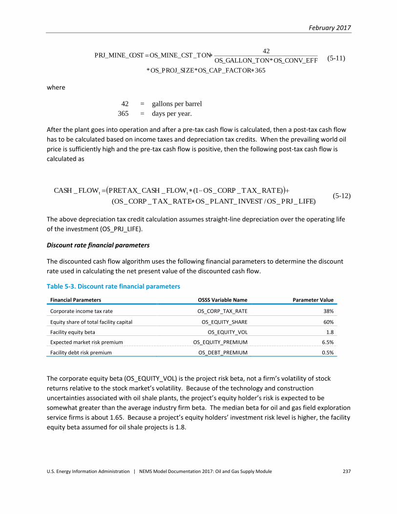
February 2017


(5-11)

where

42 = gallons per barrel

365 = days per year.

After the plant goes into operation and after a pre-tax cash flow is calculated, then a post-tax cash flow

has to be calculated based on income taxes and depreciation tax credits. When the prevailing world oil

price is sufficiently high and the pre-tax cash flow is positive, then the following post-tax cash flow is

calculated as

)LIFE_PRJ_OS/INVEST_PLANT_OSRATE_TAX_CORP_OS(

)RATE_TAX_CORP_OS1(FLOW_CASH_PRETAXFLOW_CASH tt

(5-12)

The above depreciation tax credit calculation assumes straight-line depreciation over the operating life

of the investment (OS_PRJ_LIFE).

Discount rate financial parameters

The discounted cash flow algorithm uses the following financial parameters to determine the discount

rate used in calculating the net present value of the discounted cash flow.

Table 5-3. Discount rate financial parameters

Financial Parameters OSSS Variable Name Parameter Value

Corporate income tax rate OS_CORP_TAX_RATE 38%

Equity share of total facility capital OS_EQUITY_SHARE 60%

Facility equity beta OS_EQUITY_VOL 1.8

Expected market risk premium OS_EQUITY_PREMIUM 6.5%

Facility debt risk premium OS_DEBT_PREMIUM 0.5%

The corporate equity beta (OS_EQUITY_VOL) is the project risk beta, not a firm’s volatility of stock

returns relative to the stock market’s volatility. Because of the technology and construction

uncertainties associated with oil shale plants, the project’s equity holder’s risk is expected to be

somewhat greater than the average industry firm beta. The median beta for oil and gas field exploration

service firms is about 1.65. Because a project’s equity holders’ investment risk level is higher, the facility

equity beta assumed for oil shale projects is 1.8.

365TOROS_CAP_FAC*ZEOS_PROJ_SI*

FOS_CONV_EF*TONOS_GALLON_

42T_TONOS_MINE_CSOSTPRJ_MINE_C

February 2017


The expected market risk premium (OS_EQUITY_PREMIUM), which is 6.5%, is the expected return on

market (S&P 500) over the rate of 10-year Treasury note (risk-free rate). A Monte Carlo simulation

methodology was used to estimate the expected market return.

Oil shale project bond ratings are expected to be in the Ba-rating range. Since the NEMS

macroeconomic module endogenously determines the industrial Baa bond rates for the forecasting

period, the cost-of-debt rates are different in each year. The debt premium (OS_DEBT_PREMIUM)

adjusts the bond rating for the project from the Baa to the Ba range, which is assumed to be constant at

the average historical differential over the forecasting period.

Discount rate calculation

A seminal parameter used in the calculation of the net present value of the cash flow is the discount

rate. The calculation of the discount rate used in the oil shale submodule is consistent with the way the

discount rate is calculated through NEMS. The discount rate equals the post-tax weighted average cost

of capital, which is calculated in the OSSS as follows:

))100/NS10_RMGFCM_MC)VOL_EQUITY_OS

PREMIUM_EQUITY_OS((SHARE_EQUITY_OS(

)RATE_TAX_CORP_OS1())PREMIUM_DEBT_OS

100/RMCORPBAA_MC()SHARE_EQUITY_OS1(((RATE_DISCOUNT_OS

t

tt

(5-13)

where

OS_EQUITY_SHARE = Equity share of total facility capital

100/RMCORPBAA_MC t = BAA corporate bond rate

OS_DEBT_PREMIUM = Facility debt risk premium

OS_CORP_TAX_RATE = Corporate income tax rate

OS_EQUITY_PREMIUM = Expected market risk premium

OS_EQUITY_VOL = Facility equity volatility beta

100/NS10_RMGFCM_MC t = 10-year Treasury note rate.

In calculating the facility’s cost of equity, the equity risk premium (which is a product of the expected

market premium and the facility equity beta) is added to a “risk-free” rate of return, which is considered

to be the 10-year Treasury note rate.

The nominal discount rate is translated into a constant, real discount rate using the following formula:

0.1))INFL0.1(/)RATE_DISCOUNT_OS0.1((RATE_DISCOUNT_OS ttt (5-14)

where

tINFL = Inflation rate at time t.

February 2017


Net present value discounted cash flow calculation

So far a potential project’s yearly cash flows have been calculated along with the appropriate discount

rate. Using these calculated quantities, the net present value of the yearly cash flow values is calculated

as follows:

(5-15)

If the net present value of the projected cash flows exceeds zero, then the potential oil shale facility is

considered to be economic and begins construction, so long as this facility construction does not violate

the construction timing constraints detailed below.

Oil shale facility market penetration algorithm

As noted in the introduction, there is no empirical basis for determining how rapidly new oil shale

facilities would be built, once the OSSS determines that surface-retorting oil shale facilities are

economically viable, because no full-scale commercial facilities have ever been constructed. However,

there are three primary constraints to oil shale facility construction. First, the construction of an oil

shale facility cannot be undertaken until the in-situ technology has been sufficiently developed and

tested to be deemed ready for its application to commercial size projects (i.e., 50,000 barrels per day).

Second, oil shale facility construction is constrained by the maximum oil shale production limit. Third,

oil shale production volumes cannot reach the maximum oil shale production limit any earlier than 40

years after the in-situ technology has been deemed to be feasible and available for commercial-size

facilities. Table 5-4 summarizes the primary market penetration parameters in the OSSS.

Table 5-4. Market penetration parameters

Market Penetration Parameters OSSS Variable Name Parameter Value

Earliest Facility Construction Start Date OS_START_YR 2100

Maximum Oil Shale Production OS_MAX_PROD 2 million barrels per year

Minimum Years to Reach Full Market Penetration OS_PENETRATE_YR 40

As discussed in the introduction to this submodule, oil and gas industry interest in oil shale research,

development, and production has waned in the face of the significantly greater rate of return

opportunities associated with tight oil production. The development of large-scale oil shale production

appears to be indefinitely postponed. Consequently, the Earliest Facility Construction Start Date was is

set to 2100. This parameter change effectively precludes oil shale production during the projection

period.

As discussed earlier, a 2-million-barrel-per-day oil shale production level at the end of a 40-year market

penetration period is considered to be reasonable and feasible based on the size of the resource base

RATE_DISCOUNT_OS+1

1 * tFLOW_CASH = FLOW_CASH_NET

t

t CONST_PRJ_OSLIFE_PRJ_OS

1t

1t

February 2017


and the volume and availability of water needed to develop those resources. The actual rate of market

penetration in the OSSS, however, is ultimately determined by the projected profitability of oil shale

projects. At a minimum, oil and natural gas prices must be sufficiently high to produce a facility revenue

stream (i.e., discounted cash flow) that covers all capital and operating costs, including the weighted

average cost of capital. When the discounted cash flow exceeds zero (0), then the market penetration

algorithm allows oil shale facility construction to commence.

When project discounted cash flow is greater than zero, the relative project profitability is calculated as

follows:

NVESTOS_PLANT_I / DCF OS_PROFIT tt (5-16)

where

tDCF = Project discounted cash flow at time t

NVESTOS_PLANT_I = Project capital investment

OS_PROFIT is an index of an oil project’s expected profitability. The expectation is that, as OS_PROFIT increases, the relative financial attractiveness of producing oil shale also increases.

The level of oil shale facility construction that is permitted in any year depends on the maximum oil

shale production that is permitted by the following market penetration algorithm:

) TE_YROS_PENETRA / 1989)) - YR(OS_START_ -((T*

))OS_PROFIT (1 / (OS_PROFIT * DOS_MAX_PRO MAX_PROD ttt (5-17)

where

OS_MAX_PROD = Maximum oil shale production limit

tPROFIT_OS = Relative oil shale project profitability at time t

T = Time t

OS_START_YR = First year that an oil shale facility can be built

OS_PENTRATE_YR = Minimum number of years during which the

maximum oil shale production can be achieved.

The OS_PROFIT portion of the market penetration algorithm (5-24) rapidly increases market penetration

as the DCF numerator of OS_PROFIT increases. However, as OS_PROFIT continues to increase, the rate

of increase in market penetration slows as (OS_PROFIT / (1 + OS_PROFIT) asymptotically approaches

one (1.0). As this term approaches 1.0, the algorithm’s ability to build more oil shale plants is ultimately

constrained by OS_MAX_PROD term, regardless of how financially attractive the construction of new oil

shale facilities might be. This formulation also prevents MAX_PROD from exceeding OS_MAX_PROD.

The second portion of the market penetration algorithm specifies that market penetration increases

linearly over the number of years specified by OS_PENETRATE_YR. As noted earlier OS_PENETRATE_YR

February 2017


specifies the minimum number of years over which the oil shale industry can achieve maximum

penetration. The maximum number of years required to achieve full penetration is dictated by the

speed at which the OS_PROFIT portion of the equation approaches one (1.0). If OS_PROFIT remains low,

then it is possible that MAX_PROD never comes close to reaching the OS_MAX_PROD value.

The number of new oil shale facilities that start construction in any particular year is specified by the

following equation where INT is a function that returns an integer:

TOR))OS_CAP_FAC * ZE(OS_PRJ_SI /

TOR))OS_CAP_FAC * EOS_PRJ_SIZ * (OS_PLANTS - RODINT((MAX_P NEWOS_PLANTS_ ttt

(5-18)

where

MAX_PRODt = Maximum oil shale production at time t

tPLANT_OS = Number of existing oil shale plants at time t

OS_PRJ_SIZE = Standard oil shale plant size in barrels per day

OS_CAP_FACTOR = Annual capacity factor of an oil shale plant in

percent per year.

The first portion of the above formula specifies the incremental production capacity that can be built in

any year, based on the number of plants already in existence. The latter portion of the equation

determines the integer number of new plants that can be initiated in that year, based on the expected

annual production rate of an oil shale plant.

Because oil shale production is highly uncertain, not only from a technological and economic

perspective, but also from an environmental perspective, an upper limit to oil shale production is

assumed within the OSSS. The upper limit on oil shale production is 2 million barrels per day, which is

approximately equivalent to 44 facilities of 50,000 barrels per day operating at a 90% capacity factor. So

the algorithm allows enough plants to be built to fully reach the oil shale production limit, based on the

expected plant capacity factor. As noted earlier, the oil shale market penetration algorithm is also

limited by the earliest commercial plant construction date, which is assumed to be no earlier than 2017.

While the OSSS costs and performance profiles are based on technologies evaluated in the 1970s and

early 1980s, the complete absence of any current commercial-scale oil shale production makes its future

economic development highly uncertain. If the technological, environmental, and economic hurdles are

as high or higher than those experienced during the 1970s, then the prospects for oil shale development

would remain weak throughout the projections. However, technological progress can alter the

economic and environmental landscape in unanticipated ways. For example, if an in-situ oil shale

process were to be demonstrated to be both technically feasible and commercially profitable, then the

prospects for an oil shale industry would improve significantly, and add vast economically recoverable

oil resources in the United States and possibly elsewhere in the world.

February 2017


Appendix A. Discounted Cash Flow Algorithm

Introduction

The basic DCF methodology used in the Oil and Gas Supply Module (OGSM) is applied for a broad range

of oil or natural gas projects, including single-well projects or multiple-well projects within a field. It is

designed to capture the effects of multi-year capital investments (e.g., offshore platforms). The

expected discounted cash flow value associated with exploration and/or development of a project with

oil or gas as the primary fuel in a given region evaluated in year T may be presented in a stylized form

(Equation A-1).

DCF (PVTREV PVROY PVPRODTAX PVDRILLCOST PVEQUIP

PVKAP PVOPCOST PVABANDON PVSIT PVFIT)

T

T

(A-1)

where

T = year of evaluation

PVTREV = present value of expected total revenues

PVROY = present value of expected royalty payments

PVPRODTAX = present value of expected production taxes (ad valorem and severance

taxes)

PVDRILLCOST = present value of expected exploratory and developmental drilling

expenditures

PVEQUIP = present value of expected lease equipment costs

PVKAP = present value of other expected capital costs (i.e., gravel pads and

offshore platforms)

PVOPCOST = present value of expected operating costs

PVABANDON = present value of expected abandonment costs

PVSIT = present value of expected state corporate income taxes

PVFIT = present value of expected federal corporate income taxes

Costs are assumed constant over the investment life but vary across both region and primary fuel type.

This assumption can be changed readily if required by the user. Relevant tax provisions also are assumed

unchanged over the life of the investment. Operating losses incurred in the initial investment period are

carried forward and used against revenues generated by the project in later years.

The following sections describe each component of the DCF calculation. Each variable of Equation A.1 is

discussed starting with the expected revenue and royalty payments, followed by the expected costs, and

lastly the expected tax payments.

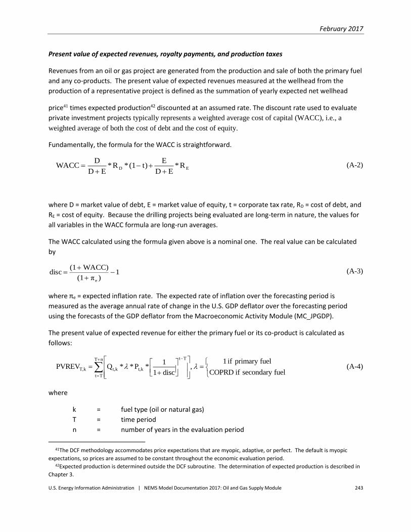
February 2017


Present value of expected revenues, royalty payments, and production taxes

Revenues from an oil or gas project are generated from the production and sale of both the primary fuel

and any co-products. The present value of expected revenues measured at the wellhead from the

production of a representative project is defined as the summation of yearly expected net wellhead

price41 times expected production42 discounted at an assumed rate. The discount rate used to evaluate

private investment projects typically represents a weighted average cost of capital (WACC), i.e., a

weighted average of both the cost of debt and the cost of equity.

Fundamentally, the formula for the WACC is straightforward.

ED R*

ED

Et)(1*R*

ED

DWACC

(A-2)

where D = market value of debt, E = market value of equity, t = corporate tax rate, RD = cost of debt, and

RE = cost of equity. Because the drilling projects being evaluated are long-term in nature, the values for

all variables in the WACC formula are long-run averages.

The WACC calculated using the formula given above is a nominal one. The real value can be calculated

by

1)π(1

WACC)(1disc

e

(A-3)

where πe = expected inflation rate. The expected rate of inflation over the forecasting period is

measured as the average annual rate of change in the U.S. GDP deflator over the forecasting period

using the forecasts of the GDP deflator from the Macroeconomic Activity Module (MC_JPGDP).

The present value of expected revenue for either the primary fuel or its co-product is calculated as

follows:

PVREV Q * *P *1

1 disc,

1 if primary fuel

COPRD if secondary fuelT,k t,k t,k

t T

t T

T n

(A-4)

where

k = fuel type (oil or natural gas)

T = time period

n = number of years in the evaluation period

41The DCF methodology accommodates price expectations that are myopic, adaptive, or perfect. The default is myopic

expectations, so prices are assumed to be constant throughout the economic evaluation period.

42Expected production is determined outside the DCF subroutine. The determination of expected production is described in

Chapter 3.

February 2017


disc = discount rate

Q = expected production volumes

P = expected net wellhead price

COPRD = co-product factor.43

Net wellhead price is equal to the market price minus any transportation costs. Market prices for oil

and gas are defined as follows: the price at the receiving refinery for oil, the first purchase price for

onshore natural gas, the price at the coastline for offshore natural gas, and the price at the Canadian

border for Alaskan gas.

The present value of the total expected revenue generated from the representative project is

PVTREV PVREV PVREVT T,1 T,2 (A-5)

where

PVREVT,1 = present value of expected revenues generated from the primary fuel

PVREVT,2 = present value of expected revenues generated from the secondary fuel.

Present Value of Expected Royalty Payments

The present value of expected royalty payments (PVROY) is simply a percentage of expected revenue

and is equal to

PVROY ROYRT *PVREV ROYRT *PVREVT 1 T,1 2 T,2 (A-6)

where

ROYRT = royalty rate, expressed as a fraction of gross revenues.

Present Value of Expected Production Taxes

Production taxes consist of ad valorem and severance taxes. The present value of expected production

tax is given by

PVPRODTAX PRREV *(1 ROYRT ) *PRDTAX PVREV

*(1 ROYRT ) *PRODTAX

T T,1 1 1 T,2

2 2

(A-7)

43The OGSM determines coproduct production as proportional to the primary product production. COPRD is the ratio of units of coproduct per unit of primary product.

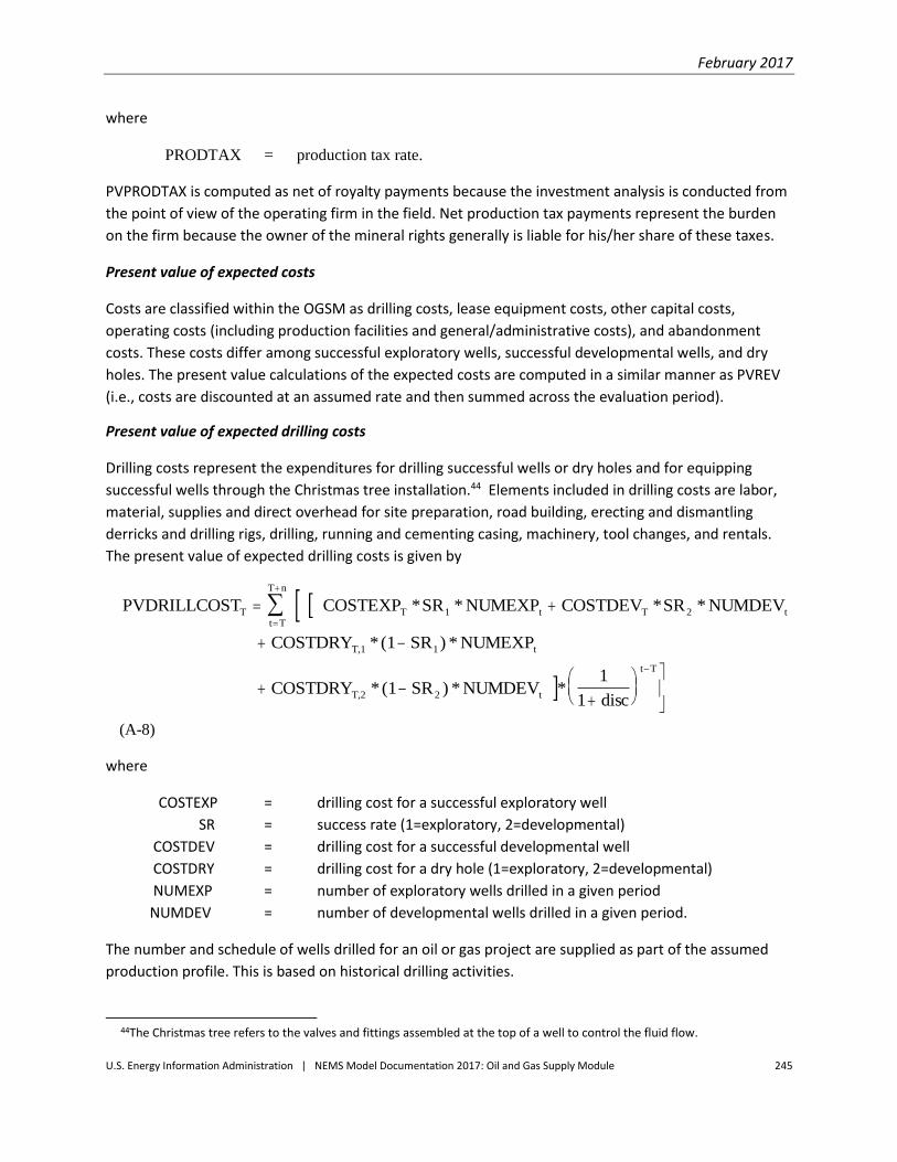
February 2017


where

PRODTAX = production tax rate.

PVPRODTAX is computed as net of royalty payments because the investment analysis is conducted from

the point of view of the operating firm in the field. Net production tax payments represent the burden

on the firm because the owner of the mineral rights generally is liable for his/her share of these taxes.

Present value of expected costs

Costs are classified within the OGSM as drilling costs, lease equipment costs, other capital costs,

operating costs (including production facilities and general/administrative costs), and abandonment

costs. These costs differ among successful exploratory wells, successful developmental wells, and dry

holes. The present value calculations of the expected costs are computed in a similar manner as PVREV

(i.e., costs are discounted at an assumed rate and then summed across the evaluation period).

Present value of expected drilling costs

Drilling costs represent the expenditures for drilling successful wells or dry holes and for equipping

successful wells through the Christmas tree installation.44 Elements included in drilling costs are labor,

material, supplies and direct overhead for site preparation, road building, erecting and dismantling

derricks and drilling rigs, drilling, running and cementing casing, machinery, tool changes, and rentals.

The present value of expected drilling costs is given by

PVDRILLCOST COSTEXP *SR * NUMEXP COSTDEV *SR * NUMDEV

COSTDRY *(1 SR ) * NUMEXP

COSTDRY *(1 SR ) * NUMDEV *1

1 disc

Tt T

T n

T 1 t T 2 t

T,1 1 t

T,2 2 t

t T

(A-8)

where

COSTEXP = drilling cost for a successful exploratory well

SR = success rate (1=exploratory, 2=developmental)

COSTDEV = drilling cost for a successful developmental well

COSTDRY = drilling cost for a dry hole (1=exploratory, 2=developmental)

NUMEXP = number of exploratory wells drilled in a given period

NUMDEV = number of developmental wells drilled in a given period.

The number and schedule of wells drilled for an oil or gas project are supplied as part of the assumed

production profile. This is based on historical drilling activities.

44The Christmas tree refers to the valves and fittings assembled at the top of a well to control the fluid flow.

February 2017


Present value of expected lease equipment costs

Lease equipment costs include the cost of all equipment extending beyond the Christmas tree, directly

used to obtain production from a drilled lease. Three categories of costs are included: producing

equipment, the gathering system, and processing equipment. Producing equipment costs include

tubing, rods, and pumping equipment. Gathering system costs consist of flowlines and manifolds.

Processing equipment costs account for the facilities utilized by successful wells.

The present value of expected lease equipment cost is

PVEQUIP EQUIP *(SR * NUMEXP SR * NUMDEV ) *1

1 discT t 1 t 2 t

t T

t T

T n

(A-9)

where

EQUIP = lease equipment costs per well.

Present value of other expected capital costs

Other major capital expenditures include the cost of gravel pads in Alaska, and offshore platforms.

These costs are exclusive of lease equipment costs. The present value of other expected capital costs is

calculated as

PVKAP KAP *1

1 discT t

t T

t T

T n

(A-10)

where

KAP = other major capital expenditures, exclusive of lease equipment.

Present value of expected operating costs

Operating costs include three main categories of costs: normal daily operations, surface maintenance,

and subsurface maintenance. Normal daily operations are further broken down into supervision and

overhead, labor, chemicals, fuel, water, and supplies. Surface maintenance accounts for all labor and

materials necessary to keep the service equipment functioning efficiently and safely. Costs of stationary

facilities, such as roads, also are included. Subsurface maintenance refers to the repair and services

required to keep the downhole equipment functioning efficiently.

Total operating cost in time t is calculated by multiplying the cost of operating a well by the number of

producing wells in time t. Therefore, the present value of expected operating costs is as follows:

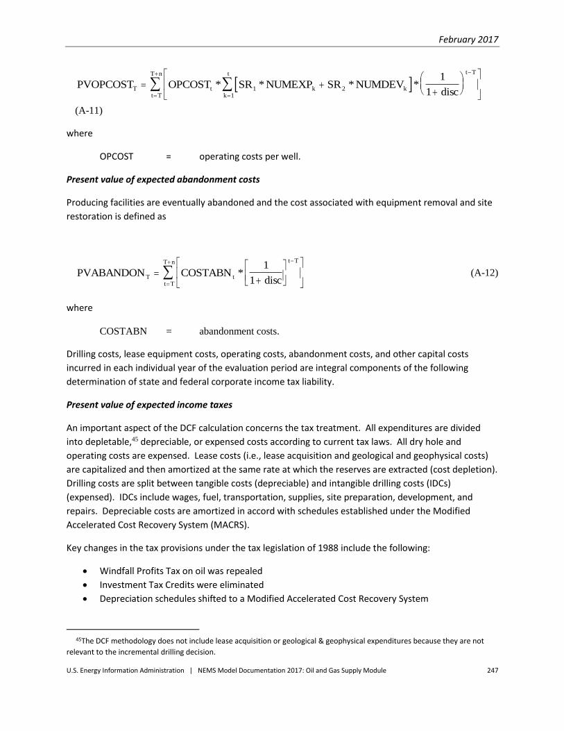
February 2017


PVOPCOST OPCOST * SR * NUMEXP SR * NUMDEV *1

1 discT t 1 k 2 kk 1

t t T

t T

T n

(A-11)

where

OPCOST = operating costs per well.

Present value of expected abandonment costs

Producing facilities are eventually abandoned and the cost associated with equipment removal and site

restoration is defined as

PVABANDON COSTABN *1

1 discT t

t T

t T

T n

(A-12)

where

COSTABN = abandonment costs.

Drilling costs, lease equipment costs, operating costs, abandonment costs, and other capital costs

incurred in each individual year of the evaluation period are integral components of the following

determination of state and federal corporate income tax liability.

Present value of expected income taxes

An important aspect of the DCF calculation concerns the tax treatment. All expenditures are divided

into depletable,45 depreciable, or expensed costs according to current tax laws. All dry hole and

operating costs are expensed. Lease costs (i.e., lease acquisition and geological and geophysical costs)

are capitalized and then amortized at the same rate at which the reserves are extracted (cost depletion).

Drilling costs are split between tangible costs (depreciable) and intangible drilling costs (IDCs)

(expensed). IDCs include wages, fuel, transportation, supplies, site preparation, development, and

repairs. Depreciable costs are amortized in accord with schedules established under the Modified

Accelerated Cost Recovery System (MACRS).

Key changes in the tax provisions under the tax legislation of 1988 include the following:

Windfall Profits Tax on oil was repealed

Investment Tax Credits were eliminated

Depreciation schedules shifted to a Modified Accelerated Cost Recovery System

45The DCF methodology does not include lease acquisition or geological & geophysical expenditures because they are not

relevant to the incremental drilling decision.

February 2017


Tax provisions vary with type of producer (major, large independent, or small independent) as shown in

Table A-1. A major oil company is one that has integrated operations from exploration and development

through refining or distribution to end users. An independent is any oil and gas producer or owner of an

interest in oil and gas property not involved in integrated operations. Small independent producers are

those with less than 1,000 barrels per day of production (oil and gas equivalent). The present DCF

methodology reflects the tax treatment provided by current tax laws for large independent producers.

The resulting present value of expected taxable income (PVTAXBASE) is given by:

PVTAXBASE TREV ROY PRODTAX OPCOST ABANDON XIDC

AIDC DEPREC DHC ) *1

1 disc

T t t t t t t

t t t

t T

t T

T n

(A-13)

where

T = year of evaluation

t = time period

n = number of years in the evaluation period

TREV = expected revenues

ROY = expected royalty payments

PRODTAX = expected production tax payments

OPCOST = expected operating costs

ABANDON = expected abandonment costs

XIDC = expected expensed intangible drilling costs

AIDC = expected amortized intangible drilling costs46

DEPREC = expected depreciable tangible drilling, lease equipment costs, and other capital

expenditures

DHC = expected dry hole costs

disc = expected discount rate.

TREVt, ROYt, PRODTAXt, OPCOSTt, and ABANDONt are the undiscounted individual year values. The

following sections describe the treatment of expensed and amortized costs for the purpose of

determining corporate income tax liability at the state and federal level.

Expected expensed costs

Expensed costs are intangible drilling costs, dry hole costs, operating costs, and abandonment costs.

Expensed costs and taxes (including royalties) are deductible from taxable income.

46This variable is included only for completeness. For large independent producers, all intangible drilling costs are expensed.

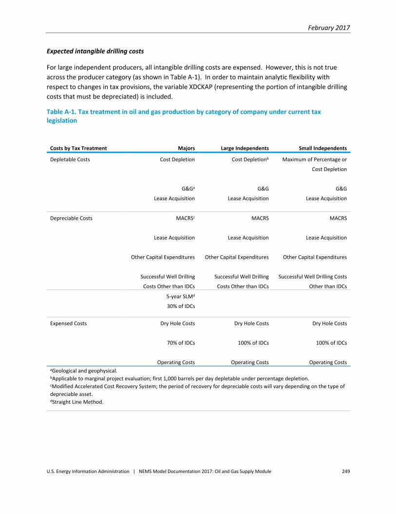
February 2017


Expected intangible drilling costs

For large independent producers, all intangible drilling costs are expensed. However, this is not true

across the producer category (as shown in Table A-1). In order to maintain analytic flexibility with

respect to changes in tax provisions, the variable XDCKAP (representing the portion of intangible drilling

costs that must be depreciated) is included.

Table A-1. Tax treatment in oil and gas production by category of company under current tax legislation

Costs by Tax Treatment Majors Large Independents Small Independents

Depletable Costs Cost Depletion

G&Ga

Lease Acquisition

Cost Depletionb

G&G

Lease Acquisition

Maximum of Percentage or

Cost Depletion

G&G

Lease Acquisition

Depreciable Costs MACRSc

Lease Acquisition

Other Capital Expenditures

Successful Well Drilling

Costs Other than IDCs

MACRS

Lease Acquisition


Successful Well Drilling

Costs Other than IDCs

MACRS

Lease Acquisition


Successful Well Drilling Costs

Other than IDCs

5-year SLMd

30% of IDCs

Expensed Costs Dry Hole Costs

70% of IDCs

Operating Costs

Dry Hole Costs

100% of IDCs

Operating Costs

Dry Hole Costs

100% of IDCs

Operating Costs aGeological and geophysical. bApplicable to marginal project evaluation; first 1,000 barrels per day depletable under percentage depletion. cModified Accelerated Cost Recovery System; the period of recovery for depreciable costs will vary depending on the type of

depreciable asset. dStraight Line Method.

February 2017


Expected expensed IDCs are defined as follows:

XIDC COSTEXP *(1 EXKAP) *(1 XDCKAP) *SR *NUMEXP

COSTDEV *(1 DVKAP) *(1 XDCKAP) *SR *NUMDEV

t T 1 t

T 2 t

(A-14)

where


EXKAP = fraction of exploratory drilling costs that are tangible and must be

depreciated

XDCKAP = fraction of intangible drilling costs that must be depreciated47


NUMEXP = number of exploratory wells


DVKAP = fraction of developmental drilling costs that are tangible and must be

depreciated

NUMDEV = number of developmental wells.

If only a portion of IDCs are expensed (as is the case for major producers), the remaining IDCs must be

depreciated. The model assumes that these costs are recovered at a rate of 10% in the first year, 20%

annually for four years, and 10% in the sixth year; this method of estimating the costs is referred to as

the 5-year Straight Line Method (SLM) with half-year convention. If depreciable costs accrue when

fewer than 6 years remain in the life of the project, the recovered costs are estimated using a simple

straight line method over the remaining period.

Thus, the value of expected depreciable IDCs is represented by

AIDC COSTEXP *(1 EXKAP) * XDCKAP *SR * NUMEXP

COSTDEV *(1 DVKAP) * XDCKAP *SR * NUMDEV

*DEPIDC *1

1 infl*

1

1 disc

T for t T m 1

t m 1 for t T m 1

t

j

t

T 1 j

T 2 j

t

t j t j

, (A-15)

47The fraction of intangible drilling costs that must be depreciated is set to zero as a default to conform with the tax perspective of a large independent firm.

February 2017


where

j = year of recovery

β = index for write-off schedule

DEPIDC = for t n+T-m, 5-year SLM recovery schedule with half-year convention;

otherwise, 1/(n+T-t) in each period

infl = expected inflation rate48

disc = expected discount rate

m = number of years in standard recovery period.

AIDC will equal zero by default since the DCF methodology reflects the tax treatment pertaining to large

independent producers.

Expected dry hole costs

All dry hole costs are expensed. Expected dry hole costs are defined as

DHC COSTDRY *(1 SR )*NUMEXP COSTDRY *(1 SR )*NUMDEVt T,1 1 t T,2 2 t (A-16)

where

COSTDRY = drilling cost for a dry hole (1=exploratory, 2=developmental).

Total expensed costs in any year equals the sum of XIDCt, OPCOSTt, ABANDONt, and DHCt.

48The write-off schedule for the 5-year SLM gives recovered amounts in nominal dollars. Therefore, recovered costs are adjusted for expected inflation to give an amount in expected constant dollars since the DCF calculation is based on constant-dollar values for all other variables.

February 2017


Table A-2. MACRS schedules

percent

Year

3-year

Recovery

Period

5-year

Recovery

Period

7-year

Recovery

Period

10-year

Recovery

Period

15-year

Recovery

Period

20-year

Recovery

Period

1 33.33 20.00 14.29 10.00 5.00 3.750

2 44.45 32.00 24.49 18.00 9.50 7.219

3 14.81 19.20 17.49 14.40 8.55 6.677

4 7.41 11.52 12.49 11.52 7.70 6.177

5 11.52 8.93 9.22 6.93 5.713

6 5.76 8.92 7.37 6.23 5.285

7 8.93 6.55 5.90 4.888

8 4.46 6.55 5.90 4.522

9 6.56 5.91 4.462

10 6.55 5.90 4.461

11 3.28 5.91 4.462

12 5.90 4.461

13 5.91 4.462

14 5.90 4.461

15 5.91 4.462

16 2.95 4.461

17 4.462

18 4.461

19 4.462

20 4.461

21 2.231

Source: U.S. Master Tax Guide.

Expected depreciable tangible drilling costs, lease equipment costs and other capital expenditures

Amortization of depreciable costs, excluding capitalized IDCs, conforms to the Modified Accelerated

Cost Recovery System (MACRS) schedules. The schedules under differing recovery periods appear in

Table A-2. The particular period of recovery for depreciable costs will conform to the specifications of

the tax code. These recovery schedules are based on the declining balance method with half-year

convention. If depreciable costs accrue when fewer years remain in the life of the project than would

allow for cost recovery over the standard period, then costs are recovered using a straight-line method

over the remaining period.

February 2017


The expected tangible drilling costs, lease equipment costs, and other capital expenditures is defined as

DEPREC (COSTEXP * EXKAP EQUIP ) *SR * NUMEXP

(COSTDEV * DVKAP EQUIP ) *SR * NUMDEV KAP

*DEP *1

1 infl*

1

1 disc

T for t T m 1

t m 1 for t T m 1

t T T 1 j

j

t

T T 2 j j

t- j+1

t j t j

, (A-17)

where

j = year of recovery

β = index for write-off schedule

m = number of years in standard recovery period


EXKAP = fraction of exploratory drilling costs that are tangible and must be depreciated

EQUIP = lease equipment costs per well


NUMEXP = number of exploratory wells


DVKAP = fraction of developmental drilling costs that are tangible and must be

depreciated

NUMDEV = number of developmental wells drilled in a given period

KAP = major capital expenditures such as gravel pads in Alaska or offshore platforms,

exclusive of lease equipment

DEP = for t n+T-m, MACRS with half-year convention; otherwise, 1/(n+T-t) in each

period

infl = expected inflation rate49

disc = expected discount rate.

Present value of expected state and federal income taxes

The present value of expected state corporate income tax is determined by

49Each of the write-off schedules give recovered amounts in nominal dollars. Therefore, recovered costs are adjusted for expected inflation to give an amount in expected constant dollars since the DCF calculation is based on constant-dollar values for all other variables.

February 2017


PVSIT PVTAXBASE *STRTT T (A-18)

where

PVTAXBASE = present value of expected taxable income (Equation A.14)

STRT = state income tax rate.

The present value of expected federal corporate income tax is calculated using the following equation:

PVFIT PVTAXBASE *(1 STRT)*FDRTT T (A-19)

where

FDRT = federal corporate income tax rate.

Summary

The discounted cash flow calculation is a useful tool for evaluating the expected profit or loss from an oil

or gas project. The calculation reflects the time value of money and provides a good basis for assessing

and comparing projects with different degrees of profitability. The timing of a project's cash inflows and

outflows has a direct affect on the profitability of the project. As a result, close attention has been given

to the tax provisions as they apply to costs.

The discounted cash flow is used in each submodule of the OGSM to determine the economic viability of

oil and gas projects. Various types of oil and gas projects are evaluated using the proposed DCF

calculation, including single-well projects and multi-year investment projects. Revenues generated from

the production and sale of co-products also are taken into account.

The DCF routine requires important assumptions, such as assumed costs and tax provisions. Drilling

costs, lease equipment costs, operating costs, and other capital costs are integral components of the

discounted cash flow analysis. The default tax provisions applied to the costs follow those used by

independent producers. Also, the decision to invest does not reflect a firm's comprehensive tax plan

that achieves aggregate tax benefits that would not accrue to the particular project under consideration.

February 2017


Appendix B. Bibliography

Aerospace Corporation. 1976. Alaska Natural Gas Transportation Systems Economic and Risk Analysis.

Advanced Resources International: “Naturally Fractured Tight Gas Reservoir Detection Optimization,”

Quarterly Status Report for U.S. DOE - METC, Contract number DE-AC21-93MC30086, May 23, 1997.

Allied Technology Group, Inc. 1996. “Model Quality Audit Report: Final Report - Oil and Gas Supply

Module.”

American Petroleum Institute. 1990-2005. Joint Association Survey on Drilling Costs, Finance,

Accounting, and Statistics Department, Washington D.C.

Argonne National Laboratory, Environmental Assessment and Information Sciences Division. June 7,

1991 (revised draft). National Energy Strategy Environmental Analysis Model (NESEAM): Documentation

and Findings, prepared for the DOE Office of Policy, Planning, and Analysis under contract

W-31-109-Eng-38.

Arps, J.J. and T.G. Roberts. 1958. "Economics of Drilling for Cretaceous Oil on East Flank of

Denver-Julesburg Basin," Bulletin of American Association of Petroleum Geologists, Vol. 42, No. 11

(November) pp. 2549-2567.

Attanasi, E.D., L.J. Drew, and D.H. Root. 1981. "Physical Variables and the Petroleum Discovery Process"

in James Ramsey, ed., The Economics of Exploration for Energy Resources (Greenwich: JAI Press).

Attanasi, E.D. and Haynes, J.L. 1983. “Future Supply of Oil and Gas from the Gulf of Mexico,” U.S.

Geological Survey Professional Paper 1294, U.S. Geological Survey.

Bacigalupi, Suzan M., et al. October 1996. Outer Continental Shelf: Estimated Oil and Gas Reserves, Gulf

of Mexico, December 31, 1995, Resource Evaluation Office, U.S. Minerals Management Service, New

Orleans.

Bailey, Ralph E. and Curtis, L.B. June 1984. Enhanced Oil Recovery, National Petroleum Council report

Submitted to the Secretary of Energy, National Petroleum Council, Washington D.C.

Baker, R.A., Gehman, H.M., James, W.R., and White, D.A. 1984. "Geologic Field Number and Size

Assessments of Oil and Gas Plays," The American Association of Petroleum Geologists Bulletin, Vol 68,

No. 4, pages 426-437.

Beach, C. and MacKimnon, J. 1978. "A Maximum Likelihood Procedure for Regression with

Autocorrelated Errors," Econometrica, Vol. 46, pages 51-58.

BehrenBruch, Peter. January 1995. Deepwater Drilling & Production: Floating Production Facilities Key to

Lower Cost Deepwater Development, HP Petroleum, Oil and Gas Journal.

February 2017


Beltramo, M., Manne a., Weyant J., The Energy Journal, 7 (July 1986), pp.15-32.

Bird, K.J. 1986. "A Comparison of the Play Analysis Techniques as Applies in Hydrocarbon Resource

Assessments of the National Petroleum Reserve in Alaska and the Arctic National Wildlife Refuge," in

Rice, D.D., ed., Oil and Gas Assessment, Methods and Applications, American Association of Petroleum

Geologists Studies in Geology, No. 21, Tulsa.

Bourgoyne Jr., A.T., et al. 1991. Applied Drilling Engineering, Society of Petroleum Engineers (SPE)

Textbook Series, Vol. 2, Second Printing, Society of Petroleum Engineers, Richardson, Texas.

Cazalet, E.G. 1977. Generalized Equilibrium Modeling: The Methodology of the SRI-Gulf Energy Model,

Decision Focus Incorporated, Palo Alto, CA and Stanford Research Institute, Menlo Park, CA.

Chapman, L. Randy, et al. November 1995. Platform/Pipeline Construction: Containing Field

Abandonment Costs in the Gulf of Mexico, Oil and Gas Journal.

Cherniavsky, E.A., and Juang, L.L. October 1979. Resource Submodels of the Long-Range Energy Analysis

Program: Documentation, Report to the Division of Long-range Analysis, U.S. Energy Information

Administration, Washington.

Cherniavsky, E.A. May 1982. "Oil/Gas Supply Modeling Considerations in Long-range Forecasting," in

Gass, S.I., Oil and Gas Supply Modeling, Proceedings of a Symposium held at the Department of

Commerce, Washington, D.C., June 18-20, 1980, U.S. Department of Commerce, NBS Special

Publication 631.

Cox, J., and Wright, A. 1976. "The Determinants of Investment in Petroleum Reserves and Their

Implications for Public Policy," American Economic Review, Vol. 66, No. 1, pages 153-167.

Cranswick, Deborah and Regg, James. February 1997. Deepwater in the Gulf of Mexico: America’s New

Frontier, OCS Report MMS 97 -0004, U.S. Minerals Management Service, New Orleans.

Davis, J.C., and Harbaugh, J.W. 1981. "A Simulation Model for Oil Exploration Policy on Federal Lands of

the U.S. Outer Continental Shelf," in Ramsey, J., ed., The Economics of Exploration for Energy Resources,

JAI Press, Greenwich.

Deacon, R., et al. 1983. The Proposed California Crude Oil Severance Tax: An Economic Analysis, The

Economics Group, Inc., Santa Barbara.

Department of Revenue, State of Alaska. 1989, 1990, and 1991. Petroleum Production Revenue Forecast.

Alaska.

Drew, L.J., Schuenemeyer, J.H., and Bawiec, W.J. 1982. Estimation of the Future Rate of Oil and Gas

Discovery in the Gulf of Mexico, U.S. Geologic Survey Professional Paper, No. 252, Reston, VA.

February 2017


DRI/McGraw-Hill, Energy Review: Natural Gas Market Focus, Standard & Poor's Corporation, Lexington, Massachusetts, 1990.

Dutton, Shirley P., Clift, Sigrid J., Hamilton, Douglas S., Hamlin, H. Scott, Hantzs, Tucker F., Howard,

William E., Akhter, M. Saleem, Laubach, Stephen E.: “Major Low-Permeability-Sandstone Gas Reservoirs

in the Continental United States,” Bureau of Economic Geology - University of Texas and Gas Research

Institute, 1993.

Eckbo, P.L., Jacoby, H.D., and Smith, J.L. 1978. "Oil Supply Forecasting: A Disaggregated Process

Approach," Bell Journal of Economics, Vol. 9, No. 1, pages 218-235.

Energy and Environmental Analysis Inc., Costs for LNG Imports Into the United States, prepared for Gas

Research Institute, GRI Contract #5087-800-1474, August 1988.

Energy and Environmental Analysis Inc. 1991. "Import and Supplemental Gas Supply," prepared for the

Source and Supply Task Group of the National Petroleum Council Natural Gas Study.

Energy Research Associates, The Reemergence of LNG - A Global Perspective, Volume I, 1989.

Epple, D. 1975. Petroleum Discoveries and Government Policy: An Econometric Study of Supply, Ballinger

Publishing Company, Cambridge, Mass.

Epple, D. 1985. "The Econometrics of Exhaustible Resource Supply: A Theory and an Application," in

Sargent, T.J., ed., Energy Foresight and Strategy, Resources for the Future, Washington.

Erickson, E.W., and Spann, R.M. 1971. "Supply Response in a Regulated Industry: The Case of Natural

Gas," The Bell Journal of Economics and Management Science, Vol. 2, No. 1, pages 94-121.

Erickson, E.W., Millsaps, S.W., and Spann, R.M. 1974. "Oil Supply and Tax Incentives," Brookings Papers

on Economic Activity, Vol. 2, pages 449-493.

Executive Office of the President. 1977. Decision and Report to Congress on the Alaska Natural Gas

Transportation System. Energy Policy and Planning.

Eyssell, J.H. "The Supply Response of Crude Petroleum: New and Optimistic Results," Business

Economics, Vol. 13, No. 3, pages 15-28.

Farmer, Richard D., Harris, Carl M., Murphy, Frederic H., and Damuth, Robert J. 1984. "The Outer

continental Shelf Oil and gas Supply model of the U.S. Energy Information Administration," North-

Holland European Journal Of Operation Research, 18.

Fisher, F.M. 1964. Supply and Costs in the United States Petroleum Industry, Johns Hopkins University

Press for Resources for the Future, Baltimore.

Fisher, W.L., et al, 1988, An Assessment of the Natural Gas Resource Base of the United States, Bureau of

Economic Geology, University of Texas at Austin, Austin, Texas.

February 2017


Gas Research Institute, Baseline Projection Data Book: The 1989 GRI Baseline Projection of U.S. Energy

Supply and Demand to 2010, Strategic Planning and Analysis Division, Washington, DC, 1990.

Frantz, Joe, “Technology Applications Improve Antrim Shale Well Recoveries and Economics,” GRI Gas

Tips, Gas Research Institute, Winter, 1995/1996, p.5-11.

Gas Research Institute, “Advanced Stimulation Technology: Success in the Anadarko Basin,” GRI Gas

Tips, Gas Research Institute, Baseline / Gas Resource Analytical Center, August, 1996.

Gas Research Institute, Baseline Projection Data Book - 1998 Edition of the GRI Baseline Projection of US

Energy Supply and Demand to 2015, Gas Research Institute, Baseline / Gas Resource Analytical Center,

1997.

Gas Research Institute, Baseline Projection Data Book - 1997 Edition of the GRI Baseline Projection of US

Energy Supply and Demand to 2015, Gas Research Institute, Baseline / Gas Resource Analytical Center,

1996.

Gas Research Institute, GRI Baseline Projection of US Energy Supply and Demand - 1997 Edition, “The

Contribution of Technology,” Gas Research Institute, Baseline / Gas Resource Analytical Center, August,

1996.

Gas Research Institute, "The Long-Term Trends in U.S. Gas Supply and Prices: The 1989 GRI Baseline

Projection of U.S. Energy Supply and Demand to 2010," as published in Gas Research Insights, Strategic

Planning and Analysis Division, Washington, DC, 1990.

Gas Research Institute (GRI). 1990. Guide to the Hydrocarbon Supply Model, prepared for the Gas

Research Institute by Energy and Environmental Analysis, Inc., Washington, DC.

Goerold, W.T. 1987. Environmental and Petroleum Resource Conflicts: A Simulation Model to Determine

the Benefits of Petroleum Production in the Arctic National Wildlife Refuge, Alaska. Materials and Society

II(3).

Goerold, W.T. 1988. A Simulation Model to Determine the Probability of Finding Economically Producible

Petroleum in the Arctic National Wildlife Refuge, Alaska, Proceedings Tenth Annual North American

Conference. International Association for Energy Economics. Houston TX.

Grecco, M.G. April 1987. Deepwater Development Economics. Offshore Technology Conference.

Griffin, James M., and Moroney, John R., Texas Severance Tax Model - The Economic Impact of

Severance Taxes: Results from an Econometric Model of the Texas Oil and Gas Industry, 1985. Report to

the Texas Mid Continent Oil and Gas Association.

Haines, Leslie. July 1996. Going Deep: Startling New Technologies and High Flow Rates Make the

Deepwater Gulf of Mexico a World Class Frontier Play - and Our Last Best Hope, Oil and Gas Investor.

February 2017


Hansen, J.J. and Kornbrath, R.W. 1986. Resource Appraisal Simulation for Petroleum in the Arctic

National Wildlife Refuge, Alaska. State of Alaska, Department of Natural Resources, Division of

Geological and Geophysical Surveys, Professional Report 90.

Harkrider, John D., Middlebrook, Mike L., Aud, William W., Marrer, Kenneth D., Teer, George A.:

“Advanced Stimulation Technology: Success in the Anadarko Basin,” GRI Gas Tips, Gas Research

Institute, Spring, 1996, p.24-29.

Helfat, Constance E. September 1989. Investment in Offshore Oil by Diversified Petroleum Companies,

Journal of Industrial Economics, Volume XXXVIII.

Hendricks, K., Novales, A. 1987. Estimation of Dynamic Investment Functions in Oil Exploration, Draft

Manuscript.

Herron, E. Hunter. June 1982. Unconventional-Gas Production Model, Final Report prepared for the

Brookhaven National Laboratory Associated Universities, Inc. by Gruy Federal Inc.

Huntington, H.G., Schuler, Glen E., et al., "North American Natural Gas Markets," Energy Modeling

Forum Stanford University, February 1989.

Huntington, H.G., Schuler, Glen E., et al., "North American Natural Gas Markets: Selected Technical

Studies," Energy Modeling Forum Stanford University, April 1989.

Huntington, H.G., Lyon, Thomas P., "Responses To Modeler Questionnaires, EMF 9: North American

Natural Gas Markets," Energy Modeling Forum Stanford University, May 1987.

ICF-Lewin Energy, Inc. June 1998. A Model for the Economic Analysis of U.S. Undiscovered Crude Oil

Resources in the Lower-48 Offshore, Prepared for U.S. Department of Energy Under Contract No. DE-

AC01-85FE60603.

ICF Resources Incorporated. August 1995. Primary Recovery Predictive Model for Total Oil Recovery

Information System (TORIS).

ICF Resources Incorporated. January 1997. Model Development for the Gas Systems Analysis Model:

Draft Topical Report, Prepared for Federal Energy Technology Center, U.S. Department of Energy, Task

4, DE-AC21-92MC28138.

ICF Resources Incorporated. January 1997. Internal Survey of Deepwater Offshore Gulf of Mexico

Projects Slated for Development, Based on Data Gathered from Various Industry Sources.

ICF Resources Incorporated. July 1990. Update and Analysis of Offshore Oil and Gas Exploration,

Development, Production and Transportation Costs, Submitted to U.S. Minerals Management Service

Under Contract No. 14-12-0001-30424.

ICF Resources Incorporated. June 1994. Update of the Regional Cost Functions for the TORIS Predictive

Models, Prepared for BDM-Oklahoma, Inc. Under Contract No. DE-AC22-94PC91008.

February 2017


International Petroleum Encyclopedia, PennWell Publishing Co., Tulsa, OK, 1989.

Johnson, D. 1985. Comparison of Alternatives for Deepwater Development in the Gulf of Mexico, SPE

Paper 13779 presented at the Hydrocarbon Economics and Evaluation Symposium, Dallas, Texas, March

14-15.

Johnson, Ronald C., Finn, Thomas M., Crovelli, Robert A., and Balay, Richard H., “An Assessment of In-

Place Gas Resources in Low-Permeability Upper Cretaceous and Lower Tertiary Sandstone Reservoirs,

Wind River Basin, Wyoming,” U.S. Geological Survey Open-File Report 96-264, U.S. Geological Survey,

1996.

Kalter, R.J., Tyner, W.E., and Hughes, D.W. 1975. Alternative Energy Leasing Strategies and Schedules for

the Outer Continental Shelf, Cornell University, Department of Agricultural Economics, A.E.RES. 75-33,

Ithaca, N.Y.

Kaufman, G.M., and Barouch, E. 1978. "The Interface Between Geostatistical Modeling of Oil and Gas

Discovery and Economics," Mathematical Geology, 10(5).

Kaufman, G.M., Runggaldier, W., and Livne, Z. 1981. "Predicting the Time Rate of Supply from a

Petroleum Play," in Ramsey, J., ed., The Economics of Exploration for Energy Resources, JAI Press,

Greenwich.

Khazzoom, D.J. "The FPC Staff's Econometric Model of Natural Gas Supply in the United States," The Bell

Journal of Economics and Managements Science, Vol. 2, No. 1, pages 51-93.

Khodaverdian, Mohamad, McLennan, John, Palmer, Ian, Vaziri, Hans: “Coalbed Cavity Completion

Analysis Suggests Improvements,” GRI Gas Tips, Gas Research Institute, Winter, 1995/1996, p.22-29.

Kibbee, Stephen. June 1996. TLP Technology: SeaStar Minimal Platform For Small Deepwater Reserves,

Atlantia Corporation, Oil and Gas Journal.

Kuuskraa, Vello A., Boyer, Charles M. III: “Economic and Parametric Analysis of Coalbed Methane,”

Hydrocarbons from Coal C AAPG Studies in Geology number38, 1993, p.373-394.

Le Blanc, Leonard. December 1995. FORECAST=96: Operators Moving Into Era of Just-In-Time

Production, Oil and Gas Journal.

Lerch, Chris, et al. February 1997. Ram-Powell Partners See Big Picture With Integrated Modeling, The

American Oil and Gas Reporter, Shell Offshore.

LNG Digest, Volume 15, Number 11, "News Briefs," Energy Research Associates, New York, November

1989.

Lore, Gary L., et al. August 1996. Summary of the 1995 Assessment of the Conventionally Recoverable

Hydrocarbon Resources of the Gulf of Mexico and Atlantic Outer Continental Shelf: As of January 1, 1995,

U.S. Minerals Management Service, New Orleans.

February 2017


Luneau, Barbara: “Accelerating Technology Development in the Greater Green River Basin”, GRI Gas

Tips, Gas Research Institute, Fall, 1995, p.4-10.

MacAvoy, P.W. and Pindyck, R.S. "Alternative Regulatory Policies for Dealing with the Natural Gas

Shortage," The Bell Journal of Economics and Management Science, Vol. 4, No. 2, pages 454-498.

MacDonald, John J. and Smith, Robert S. February 1997. Offshore Topsides: Decision Trees Aid

Production Facility Design, Oil and Gas Journal.

Mansvelt Beck, F.W., and Wiig, K.M. 1977. The Economics of Offshore Oil and Gas Supplies, Lexington

Books, Lexington, Mass.

Megill, R.E. 1988. Exploration Economics.

Melancon, J. Michael, et al. January 1997. Gulf of Mexico Outer Continental Shelf Daily Oil and Gas

Production Rate Projections from 1996 through 2000, OCS Report MMS 97-0006, Resource Evaluation

Office, U.S. Minerals Management Service, New Orleans.

Melancon, J. Michael, et al. October 1990. Outer Continental Shelf: Estimated Oil and Gas Reserves, Gulf


Orleans.

Melancon, J. Michael, et al. October 1991. Outer Continental Shelf: Estimated Oil and Gas Reserves, Gulf


Orleans.

Melancon, J. Michael, et al. September 1992. Outer Continental Shelf: Estimated Oil and Gas Reserves,

Gulf of Mexico, December 31, 1991, Resource Evaluation Office, U.S. Minerals Management Service,

New Orleans.

Melancon, J. Michael, et al. August 1993. Outer Continental Shelf: Estimated Oil and Gas Reserves, Gulf


Orleans.



Orleans.



Orleans.

Miers, John H. January 20, 1997. The Gulf of Mexico’s Revival: Technology Gives Gulf Prospects World-

Class Investment Appeal, Amoco Exploration & Production Co., Houston, Oil and Gas Journal.

February 2017


Moritis, Guntis. April 20, 1992. "EOR Increases 24% Worldwide; Claims 10% of U.S. production" [Biennial

EOR Production Report], Oil and Gas Journal, page 51 and following.

Moritis, Guntis. June 29, 1992. "More Enhanced Oil Recovery Project Information Obtained," Oil and Gas

Journal, page 70 and following pages.

Murphy, Frederic H. and William Trapmann. 1982. “An Evaluation of the Alaskan Hydrocarbon Supply

Model," Oil and Gas Supply Modeling, published by the National Bureau of Standards. Washington, DC.

National Energy Board, Canada’s Conventional Natural Gas Resources: A Status Report, Canada, April

2004.

National Petroleum Council, 1981, U.S. Arctic Oil and Gas. Energy and Environmental Analysis, Inc.

Arlington, VA.

National Petroleum Council, December 1980, Unconventional Gas Sources, Vols 1-4.

National Petroleum Council, 1984, Enhanced Oil Recovery, Washington, D.C.

National Petroleum Council, 1991, Field Development Assumptions and Costs in the Hydrocarbon Supply

Model, Energy and Environmental Analysis, Inc., Arlington, VA.

National Petroleum Council, December 1999, Natural Gas: Meeting the Challenges of the Nation’s

Growing Natural Gas Demand, Washington, DC.

National Petroleum Council, 1992, The Potential for Natural Gas in the United States, Washington, DC.

National Research Council, 1992, The National Energy Modeling System, Committee on the National

Energy Modeling System, Washington, DC.

Natural Gas Week, "DOE OKs Gas Import/Export with Mexico," June 12, 1989

Nesbitt, D., and Phillips, R. September 1980. Financial Statements and Producer Behavior in Generalized

Equilibrium Models Such as LEAP, Decision Focus Incorporated Report.

Nesbitt, D.M. 1988. Methodology of the GRI North American Regional Gas Supply-Demand Model,

Appendix A, Decision Focus Incorporated, Los Altos, CA.

Nesbitt, D.M. 1991. Insights from the North American Regional Gas (NARG) Supply-Demand Model,

Presentation to the Imports and Alaska Working Group of the National Petroleum Council Natural Gas

Study.

Newendorp, Paul, D. 1975. Decision Analysis for Petroleum Exploration, The Petroleum Publishing

Company, Tulsa, OK.

Offshore Data Services, Inc. June 1997. Database of Wells Drilled in the Deepwater Gulf of Mexico,

Houston, Texas.

February 2017


Offshore Special Report. May 1997. How Offshore Drilling Units Evolved, Offshore Magazine, Pennwell

Publications.

The Oil Daily Co., “Spot Prices on Interstate Pipeline Systems,” Natural Gas Week, 1996-1997.

Pautz, James F., et al. 1992. Enhanced Oil Recovery Projects Data Base, NIPER-583, National Institute for

Petroleum and Energy Research, Bartlesville, Oklahoma.

Petroleum Economist, Volume LVI, Number 12, "Gas Set for 1990s Growth," Euromoney Publications plc,

London, UK, December 1989.

Petroleum Economist, Volume LVI, Number 12, "Liquefied Natural Gas: Continued Market Expansion,"

Euromoney Publications plc, London, UK, December 1989.

Petroleum Information/Dwights LLC: “Production Data for the Rocky Mountain, Gulf Coast/Offshore,

and Texas/Midcontinent Areas,” Petroleum Information/Dwights LLC (CD-ROM), March 1997.

Petroleum Intelligence Weekly, Special Supplement Issue, "World LNG Trade Entering New Growth

Phase," Petroleum & Energy Intelligence Weekly, Inc., November 13, 1989.

Platt's Oilgram News, Volume 68, Number 54, "MARAD Rebuffs Cabot's $45-Million Attempt to Buy 3

LNG Tankers at Center of Dispute," McGraw-Hill, New York, March 19, 1990.

Platt's Oilgram News, Volume 68, Number 201, "LNG Ship Deal Jeopardized by New Lawsuit,"

McGraw-Hill, New York, October 16, 1990.

Potential Gas Agency, Potential Supply of Natural Gas in the United States - Report of the Potential Gas

Committee (December 31, 1996), Potential Gas Agency, March 1997.

Potential Gas Committee. 1988, Potential Supply of Natural Gas in the United States, Potential Gas

Agency, Colorado School of Mines, Golden, Colorado.

Powell, Stephen G. September 1990, Arctic National Wildlife Refuge - How Much Oil Can We Expect,

Resources Policy.

Powell, Stephen G. 1990, “A Risk Analysis of Oil Development in the Arctic National Wildlife Refuge,” The

Energy Journal, Volume 12, Number 3.

Prato, A.A., and Miller, R.R. 1981, "Evaluating the Energy Production Potential of the United States Outer

Continental Shelf," Land Economics, Vol. 57, No. 1, pages 77-90.

Riva, Joseph P., Jr., November 19, 1992, The Domestic Oil Status and a Projection of Future Production,

CRS Report for Congress, 92-826 SPR, Congressional Research Service, Washington, D.C.

February 2017


Riva, Joseph P., Jr., October 5, 1992, Domestic Oil Production, CRS Issue Brief, Order Code IB87068,

Congressional Research Service, Washington, D.C.

Roy, K.J. 1975, "Hydrocarbon Assessment Using Subjective Probability and Monte Carlo Methods," in

First IIASA Conference on Methods and Models for Assessing Energy Resources Conference, Honolulu.

Roy, K.J., Procter, R.M., and McCrossam, R.G. 1975, "Hydrocarbon Assessment Using Subjective

Probability," in Davis, J.C., Doveton, J.H., and Harbaugh, J.W., conveners, Probability Methods in Oil

Exploration: American Association of Petroleum Geologists Research Symposium Notes, Stanford,

University, pages 56-60.

Samuelson, P., "Spatial Price Equilibrium and Linear Programming," American Economic Review, 42,

1952.

Stermole, Franklin J. and Stermole, John M. 1993, Economic Evaluation and Investment Decision

Methods, Eighth Edition, Investment Evaluations Corporation, Golden, Colorado.

Trapmann, William, 1991, "Relating Natural Gas Resource Estimates to the Outlook for the Market,"

paper presented at the 14th Annual International Conference of the International Association for Energy

Economics.

Tyler, Roger, Kaiser, W.R., Scott, A.R., Hamilton, D.S., Ambrose, W.A., “Geologic and Hydrologic

Assessment of Natural Gas from Coal: Greater Green River, Piceance, Powder River, and Raton Basins,”

Bureau of Economic Geology - University of Texas and Gas Research Institute, Contract number 5091-

214-2261, 1995.

U.S. Congress, Office of Technology Assessment, 1989, Oil Production in the Arctic National Wildlife

Refuge: The Technology and the Alaskan Oil Context, OTA-E-394, Washington, D.C.

U.S. Department of Energy, 1994-2008, Costs and Indices for Domestic Oil and Gas Field Equipment and

Production Operations, Technical Report DOE/EIA-TR-0568, U.S. Energy Information Administration,

Washington D.C.

U.S. Department of Energy, “GASIS Gas Information System - A National Database of Geological,

Engineering, Production and Ultimate Recovery Data for U.S. Oil and Natural Gas Reservoirs,”

Department of Energy, GASIS Release 1 CD-ROM, March 1997.

U.S. Department of Energy, May 1997, The National Energy Modeling System: An Overview, DOE/EIA-

0581, U.S. Energy Information Administration.

U.S. Department of Energy, 1978, Midterm Oil and Gas Supply Modeling System Methodology

Description, DOE/EIA-0103/17, U.S. Energy Information Administration, Washington, DC.

U.S. Department of Energy, December 1982, Outer Continental Shelf (OCS) Oil and Gas Supply Model,

Volume 1, Model Summary and Methodology Description, DOE/EIA-0372/1, U.S. Energy Information

Administration, Washington, DC.

February 2017


U.S. Department of Energy, 1982, Outer Continental Shelf (OCS) Oil and Gas Supply Model, Volume 1,

Model Summary and Methodology Description, DOE/EIA-0372/1, U.S. Energy Information


U.S. Department of Energy, The Petroleum Resources of Mexico, DOE/EIA-0423, U.S. Energy Information

Administration, Washington, DC, 1983.

U.S. Department of Energy, 1991, Recommended Design for the National Energy Modeling System,U.S.

Energy Information Administration, NEMS Project Office, Washington, DC.

U.S. Department of Energy, 1986, An Economic Analysis of Natural Gas Resources and Supply,

DOE/EIA-0481, U.S. Energy Information Administration, Washington, DC.

U.S. Department of Energy, 1987, Potential Oil Production from the Coastal Plain of the Arctic National

Wildlife Refuge, SR/RNGD/87-01, U.S. Energy Information Administration, Washington, DC.

U.S. Department of Energy, 1988, An Assessment of the Natural Gas Resource Base of the United States,

DOE/W/31109-H1, Office of Policy, Planning & Analysis, Washington, DC.

U.S. Department of Energy, International Energy Annual 1988, DOE/EIA-0219(88), U.S. Energy

Information Administration, Washington, DC, 1988.

U.S. Department of Energy, Natural Gas Annual 1988, DOE/EIA-0131(88), U.S. Energy Information

Administration, Washington, DC, 1988.

U.S. Department of Energy, Assessment of Costs and Benefits of Flexible and Alternative Fuel Use in the

U.S. Transportation Sector; Technical Report Three: Methanol Production and Transportation Costs,

DOE/PE-0093 Office of Policy Planning and Analysis, November 1989.

U.S. Department Of Energy, 1989, Abandonment Rates of the Known Domestic Oil Resource,

DOE/BC--89/6/SP, Bartlesville Project Office, Bartlesville, Oklahoma.

U.S. Department of Energy, 1989, An Examination of Domestic Natural Gas Resource Estimates,

SR/RNGD/89-01, U.S. U.S. Energy Information Administration, Washington, DC.

U.S. Department of Energy, 1989, Federal Oil Research: A Strategy for Maximizing the Producibility of

Known U.S. Oil, DOE/FE-0139, Office of Fossil Energy, Washington, D.C.

U.S. Department of Energy, 1989, Annual Energy Review, DOE/EIA-0384(89), U.S. Energy Information


U.S. Department of Energy, 1990, The Domestic Oil and Gas Recoverable Resource Base: Supporting

Analysis for the National Energy Strategy, SR/NES/90-05, U.S. Energy Information Administration,

Washington, DC.

U.S. Department of Energy, 1990, United States Crude Oil, Natural Gas, and Natural Gas Liquids

Reserves, DOE/EIA-0216(90), U.S. Energy Information Administration, Washington, DC.

February 2017


U.S. Department of Energy, Development Costs of Undeveloped Non-associated Gas Reserves in Selected

Countries, Office of Policy Planning and Analysis, 1990.

U.S. Department of Energy, Quarterly Sales and Prices Report, Office of Fossil Energy, Office of Fuels

Programs, various issues, 1990.

U.S. Department of Energy, 1990, United States Crude Oil, Natural Gas, and Natural Gas Liquids

Reserves, DOE/EIA-0216(90), U.S. Energy Information Administration, Washington, DC.

U.S. Department of Energy, May 1991, Intermediate Future Forecasting System: Executive Summary,

DOE/EIA-M023(91) U.S. Energy Information Administration, Washington, DC.

U.S. Department of Energy, 1991, Alaska Oil and Gas Energy Wealth or Vanishing Opportunity?,

DOE/ID/01570-H1, Office of Fossil Energy, Washington, DC.

U.S. Department of Energy, 1991, The Outlook for Natural Gas Imports: Supporting Analysis for the

National Energy Strategy, SR/NES/90-06, U.S. Energy Information Administration, Washington, DC.

U.S. Department of Energy, April 1992, Model Methodology and Data Description of the Production of

Onshore Lower 48 Oil and Gas Model, U.S. Energy Information Administration, Office of Oil and Gas,

Washington, DC.

U.S. Department of Energy, 1994-2011, Documentation of the Oil and Gas Supply Module (OGSM),

DOE/EIA-M063, U.S. Energy Information Administration, Washington, DC.

U.S. Department of Energy, 1994, Documentation of the Oil and Gas Supply Module (OGSM), Appendix:

Model Developers Report, U.S. Energy Information Administration, Washington, DC.

U.S. Department of Energy, 1992, Component Design Report - Basic Framework & Onshore Lower 48

Conventional Oil and Gas Supply, U.S. Energy Information Administration, Washington, DC.

U.S. Department of Energy, 1992, Model Methodology and Data Description of the Production of

Onshore Lower 48 Oil and Gas Model, Draft Report, U.S. Energy Information Administration,

Washington, DC.

U.S. Department of the Interior, 1981, Estimates of Undiscovered Recoverable Conventional Resources of

Oil and Gas in the United States, United States Geological Survey Circular 860, United States Geological

Survey, Reston, Virginia.

U.S. Department of the Interior, 1987, Economics of Oil and Gas Production from ANWR for the

Determination of Minimum Economic Field Size, PT-87-015-3120-985, Bureau of Land Management,

Division of Mineral Resources, Alaska State Office.

U.S. Department of the Interior, 1988, National Assessment of Undiscovered Conventional Oil and Gas

Resources, USGS-MMS Working Paper, Open File Report 88-373, United States Geological Survey and

Minerals Management Service, Reston, Virginia.

February 2017


U.S. Department of the Interior, 1989, Estimates of Undiscovered Conventional Oil and Gas Resources in

the United States -- A Part of the Nation's Energy Endowment, United States Geological Survey and

Minerals Management Service, Denver, Colorado.

U.S. Department of the Interior, Federal Offshore Statistics 1990, Minerals Management Service (MMS).

U.S. Department of the Interior, Estimates of Undiscovered, Economically Recoverable Oil & Gas

Resources: for the Outer Continental Shelf, Revised as of January 1995, Minerals Management Service.

U.S. Department of the Interior, February 2006, Report to Congress: Comprehensive Inventory of U.S.

OCS Oil and Natural Gas Resources, Energy Policy Act of 2005, Minerals Management Service.

U.S. Department of the Interior, Estimates of Undiscovered, Economically Recoverable Oil & Gas

Resources: for the Outer Continental Shelf, Revised as of January 1999, Minerals Management Service.

U.S. Department of the Interior, 2008, Inventory of Onshore Federal Oil and Natural Gas Resources and

Restrictions to Their Development, United States Geological Survey.

U.S. Energy Information Administration: Annual Energy Outlook 2006 - With Projections to 2030," U.S.

Energy Information Administration, Office of Integrated Analysis and Forecasting, U.S. Department of

Energy, February, 2006.

U.S. Energy Information Administration: “U.S. Crude Oil, Natural Gas, and Natural Gas Liquids Reserves -

Annual Reports," U.S. Energy Information Administration, Office of Oil and Gas, U.S. Department of

Energy, December, 1996-2004.

U.S. Minerals Management Service, April 1996, Deepwater Royalty Relief for New Leases: Interim Rule,

30 CFR Part 260, RIN 1010-AC14, Offshore Minerals Analysis Division.

U.S. Minerals Management Service World Wide Web Page, February 1997, Database of 899 Producing

Oil and Gas Fields in the Gulf of Mexico Outer Continental Shelf.

Van Meter, John E., May 1995, Production Technology: Deciding When To Use A MOPU For Field

Development, Paragon Engineering Services, Oil and Gas Journal.

Van Poollen, H.K. and Associates, Inc., 1978, Documentation of Input Variables: Northern Alaska

Hydrocarbon Model.

Walls, M.A., 1989, Forecasting Oil Market Behavior: Rational Expectations Analysis of Price Shocks,

Resources for the Future Discussion Paper EM87-03. Washington.

Walls, Margaret A., October 1990, Analyzing the Determinants of Offshore Oil and Gas Supply: A Factual

and Methodological Assessment, Final Report Prepared for the Reserves and Natural Gas Division of the

U.S. Energy Information Administration under ORNL Subcontract No. 90X-SE635V.

Walls, Margaret A., 1990, A Survey of Oil and Gas Supply Models, Draft Report, Resources for the Future,

Washington, DC.

February 2017


Wheatley, Richard, January 20, 1997, “Deepwater, Subsalt Prospects Open New Era for Gulf of Mexico

Action,” Oil & Gas Journal.

White, D.A., and Gehman, H.M., 1979, "Methods of Estimating Oil and Gas Resources," The American

Association of Petroleum Geologists Bulletin, Vol. 63, pages 2183-2192.

White, D.A. 1980, "Assessing Oil and Gas Plays in Facies-Cycle Wedges," The American Association of

Petroleum Geologists Bulletin, Vol 64, pages 1158-1178.

White, D.A., 1981, "A Play Approach to Hydrocarbon Resource Assessment and Evaluation," in Ramsey,

J., ed., The Economics of Exploration for Energy Resources, JAI Press, Greenwich.

Williams, M.R. and Atkins, P.A., April 1987, Simple Subsea Trees for Shallow Water: An Economical

Alternative, Offshore Technology Conference.

Young, J.S. and Hauser, W.S., 1986, Economics of Oil and Gas for ANWR for the Determination of

Minimum Economic Field Size. Bureau of Land Management. Division of Mineral Resource. Alaska State

Office.

February 2017


Appendix C. Model Abstract

1. Model name

Oil and Gas Supply Module

2. Acronym

OGSM

3. Description

OGSM projects the following aspects of the crude oil and natural gas supply industry:

production

reserves

drilling activity

natural gas imports and exports

4. Purpose

OGSM is used by the Office of Energy Analysis as an analytic aid to support preparation of

projections of reserves and production of crude oil and natural gas at the regional and national

level. The annual projections and associated analyses appear in the Annual Energy Outlook

(DOE/EIA-0383) of the U.S. Energy Information Administration. The projections also are

provided as a service to other branches of the U.S. Department of Energy, the Federal

Government, and non-Federal public and private institutions concerned with the crude oil and

natural gas industry.

5. Date of last update

2013

6. Part of another model

National Energy Modeling System (NEMS)

7. Model Interface References

Coal Market Module

Electricity Market Module

Industrial Demand Module

International Energy Module

Natural Gas Transportation and Distribution Module (NGTDM)

Macroeconomic Activity Module

Liquid Fuels Market Module (LFMM)

February 2017


8. Official model representative

Office: Petroleum, Natural Gas, and Biofuels Analysis

Model Contact: Dana Van Wagener

Telephone: (202) 586-4725

9. Documentation reference

U.S. Department of Energy. 2011. Documentation of the Oil and Gas Supply Module (OGSM),

DOE/EIA M063, U.S. Energy Information Administration, Washington, DC.

10. Archive media and installation manual

NEMS2013

11. Energy Systems Described

The OGSM projects oil and natural gas production activities for six onshore and three offshore

regions as well as three Alaskan regions. Exploratory and developmental drilling activities are

treated separately, with exploratory drilling further differentiated as new field wildcats or other

exploratory wells. New field wildcats are those wells drilled for a new field on a structure or in

an environment never before productive. Other exploratory wells are those drilled in already

productive locations. Development wells are primarily within or near proved areas and can

result in extensions or revisions. Exploration yields new additions to the stock of reserves, and

development determines the rate of production from the stock of known reserves.

12. Coverage

Geographic: Six Lower 48 onshore supply regions, three Lower 48 offshore regions, and three

Alaskan regions.

Time Units/Frequency: Annually 1990 through 2040

Product(s): Crude oil and natural gas

Economic Sector(s): Oil and gas field production activities

13. Model features

Model Structure: Modular, containing four major components:

Onshore Lower 48 Oil and Gas Supply Submodule

Offshore Oil and Gas Supply Submodule

Alaska Oil and Gas Supply Submodule

Oil Shale Supply Submodule

Modeling Technique: The OGSM is a hybrid econometric/discovery process model. Drilling

activities in the United States are projected using the estimated discounted cash flow that

measures the expected present value profits for the proposed effort and other key economic

variables.

February 2017


Special Features: Can run stand-alone or within NEMS. Integrated NEMS runs employ short-

term natural gas supply functions for efficient market equilibration.

14. Non-DOE Input Data

Alaskan Oil and Gas Field Size Distributions - U.S. Geological Survey

Alaska Facility Cost By Oil Field Size - U.S. Geological Survey

Alaska Operating cost - U.S. Geological Survey

Basin Differential Prices - Natural Gas Week, Washington, DC

State Corporate Tax Rate - Commerce Clearing House, Inc. State Tax Guide

State Severance Tax Rate - Commerce Clearing House, Inc. State Tax Guide

Federal Corporate Tax Rate, Royalty Rate - U.S. Tax Code

Onshore Drilling Costs - (1) American Petroleum Institute, Joint Association Survey of Drilling

Costs (1970-2008), Washington, D.C.; (2) Additional unconventional gas recovery drilling and

operating cost data from operating companies

Offshore Technically Recoverable Oil and Gas Undiscovered Resources - Department of Interior,

Minerals Management Service (Correspondence from Gulf of Mexico and Pacific OCS regional

offices)

Offshore Exploration, Drilling, Platform, and Production Costs - Department of Interior, Minerals

Management Service (Correspondence from Gulf of Mexico and Pacific OCS regional offices)

Canadian Wells drilled - Canadian Association of Petroleum Producers, Statistical Handbook.

Canadian Recoverable Resource Base - National Energy Board, Canada’s Conventional Natural

Gas Resources: A Status Report, Canada, April 2004.

Canadian Reserves - Canadian Association of Petroleum Producers, Statistical Handbook.

Unconventional Gas Resource Data - (1) USGS 1995 National Assessment of United States Oil

and Natural Gas Resources; (2) Additional unconventional gas data from operating companies

Unconventional Gas Technology Parameters - (1) Advanced Resources International Internal

studies; (2) Data gathered from operating companies

15. DOE Input Data

Onshore Lease Equipment Cost – U.S. Energy Information Administration, Costs and Indexes for

Domestic Oil and Gas Field Equipment and Production Operations (1980 - 2008), DOE/EIA-

0815(80-08)

Onshore Operating Cost – U.S. Energy Information Administration, Costs and Indexes for

Domestic Oil and Gas Field Equipment and Production Operations (1980 - 2008), DOE/EIA-

0815(80-08)

Emissions Factors – U.S. Energy Information Administration

Oil and Gas Well Initial Flow Rates – U.S. Energy Information Administration, Office of

Petroleum, Biofuels, and Natural Gas Analysis

Wells Drilled – U.S. Energy Information Administration, Office of Energy Statistics

Expected Recovery of Oil and Gas Per Well – U.S. Energy Information Administration, Office of

Petroleum, Biofuels, and Natural Gas Analysis

February 2017


Oil and Gas Reserves – U.S. Energy Information Administration. U.S. Crude Oil, Natural Gas, and

Natural Gas Liquids Reserves, (1977-2011), DOE/EIA-0216(77-11)

16. Computing Environment

Hardware Used: PC

Operating System: UNIX simulation

Language/Software Used: Fortran

Memory Requirement: Unknown

Storage Requirement: Unknown

Estimated Run Time: 287 seconds

17. Reviews conducted

Independent Expert Review of the Offshore Oil and Gas Supply Submodule - Turkay Ertekin from

Pennsylvania State University; Bob Speir of Innovation and Information Consultants, Inc.; and

Harry Vidas of Energy and Environmental Analysis, Inc., June 2004

Independent Expert Review of the Annual Energy Outlook 2003 - Cutler J. Cleveland and Robert

K. Kaufmann of the Center for Energy and Environmental Studies, Boston University; and Harry

Vidas of Energy and Environmental Analysis, Inc., June-July 2003

Independent Expert Reviews, Model Quality Audit; Unconventional Gas Recovery Supply

Submodule - Presentations to Mara Dean (DOE/FE - Pittsburgh) and Ray Boswell (DOE/FE -

Morgantown), April 1998 and DOE/FE (Washington, DC)

18. Status of Evaluation Efforts

Not applicable

19. Bibliography

See Appendix B of this document.

February 2017


Appendix D. Output Inventory

Variable Name Description Unit Classification

Passed To

Module

OGCCAPPRD Coalbed Methane production

from CCAP

17 OGSM/NGTDM regions NGTDM

OGCNQPRD Canadian production of oil and

gas

oil: MMbbl

gas: Bcf

Fuel (oil, gas) NGTDM

OGCNPPRD Canadian price of oil and gas oil:

1987$/bbl

gas:

1987$/Bcf


OGCO2AVL CO2 volumes available MMcf 7 OLOGSS regions

13 CO2 sources

EMM

OGCO2PRC CO2 price $/Mcf 7 OLOGSS regions

13 CO2 sources

EMM

OGCO2PUR CO2 purchased from available

sources

MMcf 7 OLOGSS regions

13 CO2 sources

EMM

OGCO2PUR2 CO2 purchased at the EOR site MMcf 7 OLOGSS regions

13 CO2 sources

EMM

OGCO2TAR CO2 transport price for

interregional flows

$/Mcf 7 OLOGSS regions EMM

OGCOPRD Crude production by oil category MMbbl/day 10 OGSM reporting regions Industrial

OGCOPRDGOM Gulf of Mexico crude oil

production

MMbbl/day Shallow and deep water regions Industrial

OGCORSV Crude reserves by oil category Bbbl 5 crude production categories Industrial

OGCOWHP Crude wellhead price by oil

category

1987$/bbl 10 OGSM reporting regions Industrial

OGCRDHEAT Heat rate by type of crude oil 9 crude types LFMM

OGCRDPRD Crude oil production by OGSM

region and crude type

MMbbl/day 13 OGSM regions

9 crude types

LFMM

OGCRUDEREF Crude oil production by LFMM

region and crude type

MMbbl/day LFMM regions

9 crude types

LFMM

OGDNGPRD Dry gas production Bcf 57 Lower 48 onshore & 6 Lower 48

offshore districts

LFMM

OGELSHALE Electricity consumed Trillion Btu NA Industrial

February 2017



Passed To

Module

OGEORPRD EOR production from CO2 projects Mbbl 7 OLOGSS regions

13 CO2 sources

LFMM

OGEOYAD Unproved Associated-Dissolved gas

resources

Tcf

6 Lower 48 onshore regions

Main

OGEOYRSVON Lower 48 Onshore proved reserves by

gas category

Tcf 6 Lower 48 onshore regions

5 gas categories

Main

OGEOYINF Inferred oil and conventional NA gas

reserves

Oil: Bbbl

Gas: Tcf

6 Lower 48 onshore & 3 Lower

48 offshore regions

Main

OGEOYRSV Proved Crude oil and natural gas

reserves

Oil: Bbbl

Gas: Tcf


48 offshore regions

Main

OGEOYUGR Technically recoverable unconventional

gas resources

Tcf 6 Lower 48 onshore & 3 Lower

48 offshore regions

Main

OGEOYURR Undiscovered technically recoverable oil

and conventional NA gas resources

Oil: Bbbl

Gas: Tcf


48 offshore regions

Main

OGGROWFAC Factor to reflect expected future cons

growth

Fraction NA NGTDM

OGJOBS Number of oil and gas extraction jobs 1000s NA Macro

OGNGLAK Natural Gas Liquids from Alaska Mbbl/day NA LFMM

OGNGPLPRD Natural gas plant liquids production MMbbl/day 57 Lower 48 onshore & 6

Lower 48 offshore districts

LFMM

OGNGPRD Natural Gas production by gas category Tcf 10 OGSM reporting regions Industrial

OGNGPRDGOM Gulf of Mexico Natural Gas production Tcf Shallow and deep water

regions

Industrial

OGNGRSV Natural gas reserves by gas category Tcf 12 oil and gas categories NGTDM

OGNGWHP Natural gas wellhead price by gas

category

1987$/Mcf 10 OGSM reporting regions OGSM

OGNOWELL Wells completed Wells NA OGSM

OGPCRWHP Crude average wellhead price 1987$/bbl NA OGSM

OGPNGWHP Average natural gas wellhead price 1987$/bbl NA OGSM

OGPRCEXP Adjusted price to reflect different

expectation

NA NGTDM

OGPRCOAK Alaskan crude oil production Mbbl 3 Alaska regions NGTDM

OGPRDADOF Offshore AD gas production Bcf 3 Lower 48 offshore regions NGTDM

OGPRDADON Onshore AD gas production Bcf 17 OGSM/NGTDM regions NGTDM

February 2017



Passed To

Module

OGPRDUGR Lower 48 unconventional natural

gas production

Bcf 6 Lower 48 regions and 3

unconventional gas types

NGTDM

OGPRRCAN Canadian P/R ratio Fraction Fuels (oil, gas) NGTDM

OGPRRCO Oil P/R ratio Fraction 6 Lower 48 onshore & 3 Lower 48

offshore regions

OGSM

OGPRRNGOF Offshore non-associated dry gas

P/R ratio

Fraction 3 Lower 48 offshore regions NGTDM

OGPRRNGON Onshore non-associated dry gas

P/R ratio

Fraction 17 OGSM/NGTDM regions NGTDM

OGQCRREP Crude production by oil category MMbbl 5 crude production categories OGSM

OGQCRRSV Crude reserves Bbbl NA OGSM

OGQNGREP Natural gas production by gas

category

Tcf 12 oil and gas categories NGTDM

Macro

OGQNGRSV Natural gas reserves Tcf NA OGSM

OGQSHLGAS Natural gas production from select

shale gas plays

Bcf NA OGSM

OGQSHLOIL Crude oil production from select

tight oil plays

MMbbl NA OGSM

OGRADNGOF Non-associated dry gas reserve

additions, offshore

Bcf 3 Lower 48 offshore regions NGTDM

OGRADNGON Non-associated dry gas reserve

additions, onshore

Bcf 17 OGSM/NGTDM regions NGTDM

OGREGPRD Crude oil and natural gas

production

oil: MMbbl

gas: Bcf

6 Lower 48 onshore regions

7 fuel categories

Industrial

OGRESCO Oil reserves MMbbl 6 Lower 48 onshore & 3 Lower 48

offshore regions

OGSM

OGRESNGOF Offshore non-associated dry gas

reserves

Bcf 3 Lower 48 offshore regions NGTDM

OGRESNGON Onshore non-associated dry gas

reserves

Bcf 17 OGSM/NGTDM regions NGTDM

OGSHALENG Gas produced from oil shale Bcf NA NGTDM

OGTAXPREM Canadian tax premium oil: MMbbl

gas: Bcf


OGWELLSL48 Lower 48 drilling (successful + dry) 10 OGSM reporting regions, 7 fuel

categories

Industrial

OGWPTDM Natural Gas wellhead price 1987$/Mcf 17 OGSM/NGTDM regions NGTDM

Oil and Gas Supply Module of the National Energy Modeling ...2017).pdf · the National Energy...

Documents

Transcript of Oil and Gas Supply Module of the National Energy Modeling ...2017).pdf · the National Energy...