HSEHealth & Safety

Executive

Fracture mechanics assessmentof fatigue cracks in offshore

tubular structures

Prepared by theUniversity of Wales Swansea

for the Health and Safety Executive

OFFSHORE TECHNOLOGY REPORT

2000/077

HSEHealth & Safety

Executive

Fracture mechanics assessmentof fatigue cracks in offshore

tubular structures

D Bowness & M M K LeeUniversity of Wales Swansea

Department of Civil EngineeringSingleton Park

Swansea SA2 8PPUnited Kingdom

HSE BOOKS

ii

© Crown copyright 2002Applications for reproduction should be made in writing to:Copyright Unit, Her Majesty’s Stationery Office,St Clements House, 2-16 Colegate, Norwich NR3 1BQ

First published 2002

ISBN 0 7176 2328 9

All rights reserved. No part of this publication may bereproduced, stored in a retrieval system, or transmittedin any form or by any means (electronic, mechanical,photocopying, recording or otherwise) without the priorwritten permission of the copyright owner.

This report is made available by the Health and SafetyExecutive as part of a series of reports of work which hasbeen supported by funds provided by the Executive.Neither the Executive, nor the contractors concernedassume any liability for the reports nor do theynecessarily reflect the views or policy of the Executive.

EXECUTIVE SUMMARY

Offshore jacket structures are subjected to environmental cyclic loadings that often lead tofatigue damage, generally in the form of cracks that emanate from the weld toes at the joints.The prediction of the residual life of a fatigue damaged structure depends on a properunderstanding of the crack growth behaviour, which in turn relies on the facility to determinestress intensity factors accurately.

With the introduction of Safety Case Regulations, following Lord Cullen’s report on the PiperAlpha disaster, a Safety Case, which is renewed every three years, is required for eachinstallation operating in UK waters, to ensure that structural integrity is maintained. Thereassessment of structural integrity is therefore an important issue amongst offshore operators.Fracture mechanics analysis, using the stress intensity factor, provides the only viable means toassess the remaining fatigue life of cracked tubular joints. Also, assessing the significance of thefatigue damage allows expensive in-service inspections to be scheduled effectively, thusimproving safety. The economic benefit of a reliable fatigue crack growth analysis procedurecan thus be significant, as it enables the risk of fatigue failure to be properly evaluated, allowingexpensive repairs of damaged components to be carried out only when necessary. The results ofthis research are therefore of interest to offshore oil and gas operators and authorities enforcingoffshore safety regulations.

Despite the common occurrence of weld toe semi-elliptical surface cracks, accurate andcomprehensive stress intensity factor solutions have been lacking. Previous work has mainlyconcentrated on plane strain 2-D slices through the crack, but these edge crack solutions are notvalid for surface flaws. Although some 3-D work does exist, many assumptions were oftenmade, however, when calculating the stress intensity factors and many of the proposed solutionsare of a limited geometric applicability. These deficiencies were recognised during thedevelopment of BS 7910: 1999, which supersedes PD 6493: 1991. The research presented inthis report covers the development and assessment of a new, more comprehensive set of stressintensity factor solutions for semi-elliptical surface cracks in T-butt joints, and alsodemonstrates that they may be used for the fatigue assessment of tubular joints.

To enable the development of a new set of solutions, a very extensive parametric study ofcracked plates and T-butt joints was conducted. In this study, the effects of the weld geometry—weld angle, attachment footprint width and weld toe grinding—as well as those due to the crackdepth and aspect ratio were investigated. The results from the parametric study were used tocompile a database of weld toe magnification factors, which describe the effect of the weldedattachment on the stress intensity factors relative to the same crack in a plate.

Using the database, estimation equations for the weld toe magnification factor were developedfrom multiple, non-linear regression analyses. The accuracy of fit of the equations was assessedby examining the regression statistics and plotting histograms of the percentage error of theequation predictions relative to the database values. Visual comparisons were also carried out byplotting graphs of the equations alongside the database values. The assessment demonstratesthat the equations are a very good fit to the data from which they were derived. With regard tothe validity of the new equations, a discussion of the validity limits is given in this report andrecommendations are made. The resulting equations, used in conjunction with existing platesolutions, provide new stress intensity factor solutions for cracked T-butt joints.

To assess the new solutions, comparisons were firstly made with some of the more importantexisting solutions. Following this, a more detailed investigation was conducted in which thenew solutions were used to predict stress intensity factors for cracks in tubular joints. Due to the

iii

fact that only a limited number of tubular joint stress intensity factors are reported in theliterature, a numerical study of various tubular joint geometries and configurations was initiallyperformed to generate data for comparison. The comparisons show that for shallow and narrowcracks—depths of up to 10% of the chord wall thickness and a total width of up to six times thechord wall thickness—the T-butt joint solutions, in conjunction with the geometric hot spotstress and degree of bending, can yield stress intensity factors in very close agreement withthose for tubular joints. They also show that the hot spot stress must be evaluated usingquadratic extrapolation to obtain this good agreement because linear extrapolation underpredictsthe actual stress magnitude.

For deep and wide cracks, the new solutions yield conservatively high stress intensity factors.At the deepest point of the crack, the conservatism is due to the differences in load sheddingbetween T-butt joints and tubular joints. Whereas the discrepancy at the crack ends was shownto be due to the intersection stress distribution, which falls away with distance from the hot spotlocation—using the stress field local to the position of the crack ends was found to producemore accurate stress intensity factors.

As a final assessment of the new solutions, they were used to perform numerous fatigue crackgrowth calculations, and the resulting fatigue lives were compared with the current designstress-endurance curve as well as experimental results in a fatigue database. In the first part ofthis assessment, the effects of the various input parameters used in fatigue life calculations wereinvestigated. This showed that the weld angle, weld toe grinding, the degree of bending and thechord wall thickness all have a particularly marked effect on the calculated fatigue life. Whenused to calculate the lives of joints in the experimental fatigue database, the new solutions wereseen to yield conservative results of around half of the experimental lives. Further investigationdemonstrated that this discrepancy was probably due to load redistribution and the intersectionstress distribution in the tubular joints, although it is noted that the crack initiation phase cannotbe predicted by fracture mechanics. The new solutions did, however, perform very well withregard to capturing trends in the fatigue database, yielding results which significantly reducedthe dependency on the tubular joint loading mode exhibited by results in the database.

iv

v

ACKNOWLEDGEMENTS

The authors would like to acknowledge the financial support of the Engineering and PhysicalSciences Research Council, The Health and Safety Executive and Chevron Oil.

vi

CONTENTS

Executive Summary iii

Acknowledgements v

Contents vii

1. INTRODUCTION AND BACKGROUND 1

2. NUMERICAL MODELLING OF 3-D T-BUTT JOINTS 32.1 Mesh generation 32.2 Analysis 6

3. SIF AND Mk FACTOR EVALUATION 93.1 Calculation of SIFs by displacement extrapolation 93.2 Calculation of SIFs from the J-integral 103.3 Calculation of the shape factor Y 113.4 Calculation of the Mk factor 14

4. PARAMETER RANGES FOR THE PARAMETRIC STUDY 154.1 Crack dimensions 154.2 Weld dimensions 154.3 Joint dimensions 17

5. PARAMETRIC STUDY RESULTS AND DISCUSSION 195.1 Breakdown of parametric study analyses 195.2 Comparison of SIF evaluation methods 195.3 Results from the ‘base’ parametric study 215.4 Typical results from the main parametric study 27

6. THE DEVELOPMENT OF NEW Mk FACTOR EQUATIONS 416.1 Regression of data 416.2 Development of the new equations 416.3 Data used in the regression analyses 476.4 The resulting regression equations 48

7. ASSESSMENT OF THE REGRESSION EQUATIONS 577.1 Statistical evaluation 577.2 Error frequency distributions 587.3 Visual assessment of the regression equations 65

8. VALIDITY OF THE REGRESSION EQUATIONS 738.1 Validity limits of the equations 738.2 Other validity limit issues 778.3 Conclusions on the validity of the equations 79

9. COMPARISONS WITH EXISTING Mk / SIF SOLUTIONS 819.1 Plain plate SIF solutions of Newman and Raju 819.2 Edge crack Mk factors of BS 7910 849.3 3-D T-butt joint Mk factors of Bell 869.4 3-D T-butt joint SIF solutions of Brennan et al. 909.5 Tubular T-joint SIF solutions of Rhee et al. 90

vii

10. COMPARISONS WITH TUBULAR JOINT SIFs 9710.1 Numerical modelling of cracked tubular joints 9710.2 Prediction of tubular joint SIFs from T-butt joint solutions 10410.3 Correlation between tubular joint and T-butt joint SIFs 110

11. FATIGUE CRACK GROWTH CALCULATIONS USING THE NEW SIFSOLUTIONS 16111.1 Basic procedure for performing crack growth calculations 16111.2 Factors affecting the calculated fatigue life 16111.3 Comparison with the HSE 16mm tubular T-joint database 182

12. CONCLUSIONS 187

13. REFERENCES 189

Appendix A – Database of Mk factors 191

Appendix B – The New Mk factor Solutions 239

viii

1

1. INTRODUCTION AND BACKGROUND

The use of T-butt joints to calculate stress intensity factors (SIFs) for weld toe cracks in tubularjoints has been proposed by many researchers, including Dijkstra et al. (TNO, Delft), Pang(Nanyang Technological University), Fu et al. (British Gas), Maddox (TWI) and Burdekin et al.(UMIST). The reasons for using T-butt joint solutions to approximate tubular joint SIFs are,first, because tubular joint solutions only exist for a few very basic tubular joint configurations,and, secondly, because to derive solutions for the many different geometries and configurationsof tubular joint used in practice would require an unmanageable number of analyses.

T-butt joint SIFs are chosen because the geometry of a T-butt joint is in effect an ‘unwrapped’tubular intersection. Using the uncracked SCF and DOB (degree of bending) at the cracklocation in the tubular joint, the SIF for a crack in that joint may be approximated from T-buttjoint solutions as

( )[ ]K Y SCF DOB Y SCF DOB am b nomtubular joint ≈ − +. . . .1 σ π (1)

where Ym and Yb are the shape factors for a crack in a T-butt joint under membrane and bendingloading, respectively, σnom is the nominal stress in the reference brace of the tubular joint and ais the crack depth. In this approximation, the effect of the weld and the attachment on the crackis primarily derived from the T-butt joint solutions whilst the tubular joint geometry andconfiguration are accounted for in the SCF and the DOB.

The accuracy of the calculated SIF is dependent on two factors. The first is the applicability ofT-butt joint solutions to tubular joints, i.e. how well the T-butt joint simulates the crack planeconditions experienced by the crack in a tubular joint. The second factor is the T-butt jointsolutions themselves, as those that currently exist are either inaccurate since they are based onapproximations, some of which are incorrect, or only have limited validity ranges. The workpresented in this report aims to solve this second factor by developing new, widely applicable,accurate equations for the weld toe magnification factor. The weld toe magnification factor,after Maddox (1975), describes the effect of a welded attachment on a crack and is defined by

MkY

Y= ( )

( )

in plate with attachment

in same plate but with no attachment

(2)

Hence, the T-butt joint shape factors in equation (1) may be calculated from

Y Y Mk(T butt) (plain plate)− = (3)

and so the predicted tubular joint stress intensity factor becomes

( )[ ] aDOBSCFMMkDOBSCFMMkK nombbmm πσ+−≈ ...1...jointtubular (4)

where Mm and Mb are the shape factors for a crack in a plain plate under membrane and bendingloading, respectively.

This report details the development of new equations for the weld toe magnification factor. Itbegins with a description of the finite element models used to evaluate the stress intensityfactors for semi-elliptical weld toe cracks in T-butt joint geometries. Details of the parametricstudy, in which a database (Appendix A) of weld toe magnification factors was derived, are

2

given. These data were then regressed into equation form, and the development and assessmentof these equations is described in some detail. The resulting new equations are presented, intheir final form, in Appendix B at the rear of this report.

In the final part of the report, the new solutions are assessed, firstly, by comparison with someof the more important existing Mk factor and SIF solutions. A detailed comparison betweentubular joint and T-butt joint SIFs is then carried out. Finally, the new solutions are used toperform fatigue crack growth calculations and to predict the lives of tubular joint specimens.

3

2. NUMERICAL MODELLING OF 3-D T-BUTT JOINTS

2.1 MESH GENERATION

The starting block in the creation of a 3-D T-butt joint model is a plain plate mesh containing asemi-elliptical surface crack. To generate this plain plate, the software ABACRACK (1989) isused. A typical mesh, along with a close-up of the mesh in the region of the crack tip, is shownin Figure 1. This shows a spider’s web type mesh configuration radiating from the semi-elliptical crack front. To generate an ABACRACK mesh, an input file must be prepared whichcontains 18 parameters controlling the dimensions, grading and other details. The length andwidth of the plate, and the width and depth of the crack are normalised by the plate thickness,which is always unity.

The FORTRAN program ABABUTT, which was developed at Swansea (Bowness, 1996), usesthe plain plate mesh created by ABACRACK and turns it into a T-butt joint. The intermediatesteps in this process are illustrated in Figure 2. Firstly, an attachment of uniform thickness isadded to the top of the plain plate mesh (Figure 2b). (The number of elements through thethickness of the attachment, the thickness of the first element layer at the weld toe, and the meshgrading are controlled by user input parameters.) The next stage is to map the attachment to givethe desired attachment thickness and weld profile (Figure 2c). User input parameters govern thethickness of the attachment and the overall attachment footprint length. To achieve thesedimensions and to maintain the nodal connectivity between the plate and the attachment, the co-ordinates of the nodes within the plain plate are adjusted. With regard to the weld, the user candefine the global weld angle as well as the radius of the weld toe. Finally, the main plate mesh isreflected, resulting in a 3-D T-butt joint with a semi-elliptical weld toe crack (Figure 2d).

The unsymmetrical geometry of a T-butt joint causes the crack to curve slightly under the weldtoe as it grows through the main plate (Wildschut et al., 1987). If known, this curvature can bemodelled by ABABUTT. In the work reported here, however, all cracks are modelledperpendicular to the main plate. Note that ignoring crack curvature does not adversely affect thecalculated SIFs (Bowness and Lee, 1998).

As well as generating the mesh, ABABUTT creates ready-to-run input data decks compatiblewith the finite element code ABAQUS (1996), used for the analyses. Also, files necessary forpostprocessing (SIF evaluation) are produced. This fully automated process considerablyreduces the effort required to create numerical models of 3-D T-butt joints, making it possible tocarry out the extensive parametric study that forms the core of this project.

4

(a) quarter plain plate mesh

(b) close-up of crack front mesh

Figure 1A typical ABACRACK mesh

5

(a) quarter plain plate mesh fromABACRACK

(b) add attachment

(c) map attachment to desiredgeometry and weld profile

(d) reflect the plain plate mesh to form a half T-butt joint

Figure 2ABABUTT modelling sequence

6

2.2 ANALYSIS

The element type chosen for the analyses was the reduced integration 20-noded brick C3D20Rfrom the ABAQUS (1996) element library. At the crack front, the brick elements were collapsedto wedges with the midside nodes placed at the halfway points; the use of the quarterpointtechnique, to force the element to have a 1/√r strain variation, was found previously to have anegligible effect on the results (Bowness, 1996). This is due to the very fine crack tip meshesused for the work presented here – the width of the crack tip elements is around 0.01T, or less.In fact the quarterpoint technique can be detrimental because if the ring of singularity elementsis not optimally sized, the technique will introduce errors into the solution (Harrop, 1982).Moreover, the results presented later in this report reveal that, for certain crack geometries andat some of the positions on the crack front, the strain does not vary according to 1/√r.

Each model was analysed under membrane and bending loading. For membrane loading, oneend of the main plate was restrained whilst the other was given a uniform longitudinaldisplacement. There are many ways to load a T-butt joint in bending, but the closest to theconditions experienced at a tubular intersection is thought to be three-point bending where theattachment is loaded. Thus, the ends of the main plate were restrained and a displacement wasapplied to the end of the attachment. A deformed model under bending loading is shown inFigure 3 along with a close-up of the opened crack. Bending loading for the plain plate wasachieved via pure bending.

The Young’s modulus and the Poisson’s ratio used in the analyses were 210 kNmm-2 and 0.3,respectively. The elastic finite element calculations were performed using the general purposefinite element package ABAQUS (1996). For the most refined models which contained around8500 20-noded brick elements (over 110,000 degrees of freedom), solution times were around50 cpu minutes using the sparse solver on a SUN Ultra 2170, although more typical modelscontaining about 2500 brick elements took less than 10 minutes of cpu time.

7

(a) general view of deformed half model

(b) close-up of the opened crack

Figure 3Deformed T-butt joint model under bending loading

8

9

3. SIF AND Mk FACTOR EVALUATION

Several well established procedures exist for evaluating stress intensity factors in arbitrarycracked bodies. Currently, the most popular method is probably the virtual crack extension,which is implemented in ABAQUS (1996) to provide estimates of the J-integral. It has theadvantage of being rather insensitive to mesh refinement and is applicable for elastic and plasticmaterial behaviour. Fu et al. (1993), however, in their 3-D T-butt joint analyses, noted a lack ofpath independence in the region where the crack meets the weld toe. They attributed this to thepresence of two stress singularities – one due to the weld toe and the other the crack tip – at thispoint, and later, Kristiansen and Fu (1993) recommended the method of displacementextrapolation for 3-D T-butt joint SIF evaluation. Due to the lack of any clear guidance on SIFevaluation, SIFs are calculated using both the virtual crack extension and displacementextrapolation techniques in the work reported here.

As mentioned earlier, cracks in the current work are modelled perpendicular to the main plate.Since, in reality, cracks curve under the weld toe, this approximation will induce shearing modeSIFs that may need to be accounted for. Results from the virtual crack extension willautomatically include the effect of shearing modes. With displacement extrapolation, each modemust be evaluated separately and combined in some way.

3.1 CALCULATION OF SIFs BY DISPLACEMENT EXTRAPOLATION

In order to apply the displacement extrapolation technique to a semi-elliptical crack, the localradial (r), normal (n) and tangential (t) directions must be defined for each point on the crackfront. This is achieved by calculating the vectors defining these local directions for theABACRACK plain plate mesh; this is quite straightforward as the crack is planar and lies in aglobal co-ordinate plane. The radial direction is calculated from the co-ordinates of the nodes onthe radial paths which cross the crack front. The tangential direction is determined from thederivative of the equation defining the elliptical crack front. The third vector, in the normaldirection, is then simply generated from a cross product of the other two. Using these vectors,local direction cosines may be calculated, allowing the global displacements from the finiteelement analyses to be transformed into local displacements according to

u

v

w

l m n

l m n

l m n

U

V

W

r

n

t

=

1 1 1

2 2 2

3 3 3

(5)

where ur, vn, wt are the local radial, normal and tangential displacements, U, V, W the globaldisplacements and l1, m1, n1 etc. the direction cosines of the local directions with respect to theglobal axes.

To evaluate the mixed mode stress intensity factors, the largest displacements in the vicinity ofthe crack, obtained from the radial paths up the crack face, were chosen. And due to theunsymmetrical nature of the problem about the crack plane, radial paths up both the crack faceswere used. The SIF was then taken to be the average of the values calculated for each crackface. Using the displacements on the crack faces also means that the Westergaard equations, forthe displacements in the vicinity of a crack tip, reduce to

10

( )vK

G

rn

I= −2

2 2π

υ (6)

( )uK

G

rr

II= −2

2 2π

υ (7)

wK

G

rt

III=2π

(8)

for plane strain, where G is the elastic shear modulus (= E/[2(1+υ)]) and all the otherdisplacements become zero. For plane stress, υ must be replaced with υ/(1+υ) in the equations.Because these equations are only valid close to the crack tip, results from the first three brickelements were used for the extrapolation back to the tip. However, results from the collapsedbrick adjacent to the tip were ignored, since at the crack tip the SIFs produced by equations (6)–(8) are infinite and the next two nodes are prone to numerical errors.

Another consideration when implementing the displacement extrapolation technique waswhether the plane stress or plane strain form of equations (6)–(8) should be used to convert thedisplacements into stress intensity factors. Newman and Raju (1979), in their analysis of semi-elliptical cracks in plain plates, used a nodal force method to calculate stress intensity factorswhich required no assumption. For plain plate cracks, it is generally accepted that plane strainconditions exist everywhere along the crack front apart from where the crack meets the freesurface. Fu et al. (1993), in their work on 3-D T-butt joints, assumed plane strain everywherewhereas Kristiansen and Fu (1993), having examined in detail the area where the crack meetsthe weld toe, concluded, not surprisingly, that the condition was somewhere between planestress and plane strain because of the restraint provided by the attachment. In this project, planestrain conditions are assumed everywhere except for the crack end location in plain plates wherethe SIFs are calculated using plane stress.

To take into account the shearing mode stress intensity factors, an effective SIF was defined as

( )K K KK

eff I IIIII= + +

−2 2

2

21 υ(9)

This combination, which is used in the treatment of mixed mode SIFs in the CEGB R6 method(Milne et al., 1986), was found to be adequate in previous work conducted at Swansea(Bowness, 1996). One final complication, brought about by using equation (9), is that the signof Keff will not become negative if the crack closes – this is possible for deep round crackswhere the deepest point lies below the neutral surface. Hence, the sign of Keff is taken to be thesame as that of KI such that

( )KK

KK K

Keff

I

II II

III= + +−

2 22

21 υ(10)

3.2 CALCULATION OF SIFs FROM THE J-INTEGRAL

The virtual crack extension technique, implemented in ABAQUS (1996) was used to provideestimates of the J-integral. In the elastic regime, the SIF may be calculated from the J-integralvalue as

11

K JE= (11)

for plane stress. For plane strain, E must be replaced with E/(1-υ2). For each crack front node,four contours were requested, each representing one ring of crack front elements. Then, usingequation (11), the contour values were converted to SIFs. Each crack front node SIF was thentaken to be the average of those calculated from contours 2, 3 and 4, with the first contour,which is prone to numerical error, being ignored.

With regard to the use of the plane stress or plane strain form of equation (11), as withdisplacement extrapolation, plane strain was used everywhere with the exception of the crackends in plain plates. Also, the sign of the J-integral provided by ABAQUS does not change asthe crack closes, so in the same way that the sign of equation (10) is determined from theopening mode SIF, equation (11) must be calculated as

KK

KJEI

I= (12)

where KI is calculated by displacement extrapolation.

3.3 CALCULATION OF THE SHAPE FACTOR Y

Once the SIFs have been evaluated, it is necessary to non-dimensionalise them with respect toloading and absolute crack length. These non-dimensional SIFs, or shape factors (Y), arecalculated according to

YK

anom=

σ π(13)

where σnom is the nominal stress in the main plate and a is the absolute crack depth. Thecalculation of the nominal stress in the main plate in a T-butt joint is a relatively simple task,requiring only a basic knowledge of statics. When the main plate is cracked, however,significant differences in the nominal stress may occur depending on how the nominal stress iscomputed. For instance, if the T-butt joint is loaded in tension by applied displacement,knowing the length of the main plate, the strain and hence nominal stress may be computed; thisis effectively an uncracked nominal stress. But a different nominal stress may be calculated ifthe reaction, where the displacement is applied, is divided by the plate cross-sectional area; thisnominal stress includes the reduction in stiffness of the plate due to the presence of the crack. Athird nominal stress could also be defined by dividing the reaction by the area of the plate minusthe cracked area – a net section nominal stress.

In this project, all models are displacement loaded and the uncracked nominal stresses are used.The choice of this method of nominal stress calculation is for consistency with the way the SIFsolutions will be used, i.e. tubular joint SIFs will be approximated by using the uncracked SCFand DOB (see equation (1)). Hence, with reference to Figure 4, the nominal stress for membraneloading is

σ δnom E h= / 2 (14)

where δ is the applied displacement. With a small L/T, the displacement applied to the end ofthe main plate mesh is shared almost evenly between the two halves of the main plate, i.e. theside with the attachment and the plate side both extend by δ/2, and so equation (14) may be used

12

directly. But when L/T is large, e.g. 2.0 and 2.75, the less stiff plain side of the main plateextends by more than δ/2, and so the nominal stress must be calculated by using a δ equal to 2times the extension of the plate half; this may be evaluated from the displacements half wayalong the plain plate.

Figure 4Nomenclature for a half 3-D T-butt joint

For bending loading, assuming the axial stiffness of the attachment is much greater than thebending stiffness of the main plate, the nominal stress is

σ δnom E h= 1 5 2. / (15)

However, for the T-butt joints with thin attachments, for example L/T = 0.5, the extension of theattachment can mean that the displacement at the base of the attachment, i.e. the displacement inthe centre of the main plate, is significantly less than the displacement δ applied to the end ofthe attachment. Thus, the nominal stress is less than that calculated from equation (15). Thenominal stress for bending should, therefore, be calculated by using a δ evaluated from thedisplacement at the base of the attachment in the centre of the main plate.

To test the accuracy of the methods described above for calculating the nominal stresses, fouruncracked T-butt joints with different attachment footprint widths were analysed undermembrane and bending loadings, to evaluate the stress distributions on the plain side of themain plate. The results are shown in Figure 5. The SCF was calculated by dividing the actualstress, obtained from the finite element analysis, by the theoretical nominal stress, computed asdescribed above. As one would expect, the SCF increases rapidly as the weld toe is approached,but away from the weld toe the SCF converges on that computed theoretically.

13

0.0

0.5

1.0

1.5

2.0

2.5

3.0

3.5

0 0.2 0.4 0.6 0.8 1 1.2

Distance from weld toe / T

SC

FL/T = 0.5L/T = 1.25L/T = 2.0L/T = 2.75Theoretical nominal stress

(a) membrane loading

0.0

0.5

1.0

1.5

2.0

2.5

3.0

3.5

0 0.2 0.4 0.6 0.8 1 1.2

Distance from weld toe / T

SC

F

L/T = 0.5L/T = 1.25L/T = 2.0L/T = 2.75Theoretical nominal stress

(b) bending loading

Figure 5Distribution of the SCF perpendicular to the crack plane with distance from the weld toe

14

3.4 CALCULATION OF THE Mk FACTOR

Once the shape factors have been calculated, the weld toe magnification factor (Mk) may becalculated by dividing the T-butt joint Y factor by the plain plate Y factor, according to equation(2).

15

4. PARAMETER RANGES FOR THE PARAMETRIC STUDY

This section details the choice of T-butt joint and crack geometries covered in the parametricstudy.

4.1 CRACK DIMENSIONS

4.1.1 Crack depth - a/T = 0.005, 0.01, 0.02, 0.04, 0.07, 0.1, 0.2, 0.3, 0.5, 0.7, 0.9

During fatigue crack growth, most of the propagation life is consumed whilst the crack is veryshallow. At this critical stage, the effect of the weld toe is most pronounced, which is reflectedin the rapidly rising Mk factors with decreasing crack depth. Hence, the smallest a/T in theparametric study was selected to be 0.005, representing a crack of depth 0.25mm in a 50mmplate. This is in accordance with the initial flaw depth suggested when considering failure at theweld toe of an otherwise undefective weld (HSE, 1995b). With regard to the deepest crackdepth, a/T = 0.9 is proposed as it is the deepest semi-elliptical crack depth that may bepracticably modelled. The suggested intermediate crack depths are concentrated on where thegradient of Mk is the highest.

4.1.2 Crack aspect ratio - a/c = 0.1, 0.2, 0.4, 0.7, 1.0

The proposed crack aspect ratios cover most defect sizes experienced in real tubular joints: froma semi-circular crack to one where the total width is 20 times the depth.

4.2 WELD DIMENSIONS

4.2.1 Attachment footprint - L/T = 0.5, 1.25, 2.0, 2.75

The attachment footprint widths proposed are consistent with the AWS D1.1-90 (1990)recommendations for standard flat and toe fillet weld profiles. To derive typical L/T values,tubular joint τ-ratios of 0.5 and 1.0 were considered with chord thicknesses of 16, 32 and 50mm.Combinations of τ and T were then input into the equations given in Table 1, which summarisethe AWS prequalified weld size details.

16

Table 1Attachment footprint length (L) for an AWS prequalified weld

AWS Detail “A” Detail “B” Detail “C”Figure ΨΨ = 180° -135° ΨΨ = 135° -90° ΨΨ = 90° -50° ΨΨ = 75° -30°

10.9(stand.

flat)

L tb≥ sin Ψbut need not be> 1 75. tb

( )L t Fw≥ + sin Ψwheret tw b≥F

tb

= −( .

. )

1 5

0 01111Ψ

( )L t Fw≥ +wheret tw b≥ sin ΨF tb= 2

( )L t Fw≥ +wheret tw b≥ sin Ψbut need not be> 1 75. tb

F tb= 2

10.10(toe

fillet)

L tb≥ sin Ψbut need not be> 1 75. tb ( )

Lt

F

w≥ +

−sin

.4 sin

sin

ΨΨ

Ψ1 90 2

�

wheret tw b≥F tb= 2

( )L t Fw≥ +wheret tw b≥ sin ΨF tb= 2

( )L t Fw≥ +wheret tw b≥ sin Ψbut need not be> 1 75. tb

F tb= 2

Table 2 shows the calculated values of L and L/T for various local dihedral angles Ψ, i.e.intersection locations.

Table 2Calculated attachment footprint widths

Ψ Ψ = 180° 150° 120° 90° 60° 30°Weld detail “A” “A” “B” “B” “B” “C”

T tb L (mm)(mm) (mm) Weld type L/T

16 8 standard flat 14.00 14.00 10.78 12.00 13.24 18.000.875 0.875 0.674 0.75 0.828 1.125

16 16 standard flat 28.00 28.00 21.56 24.00 26.48 36.001.75 1.75 1.348 1.5 1.655 2.25

16 16 toe fillet 28.00 28.00 24.94 24.00 26.48 36.001.75 1.75 1.559 1.5 1.655 2.25

32 16 standard flat 28.00 28.00 21.56 24.00 26.48 36.000.875 0.875 0.674 0.75 0.828 1.125

32 16 toe fillet 28.00 28.00 24.94 24.00 26.48 36.000.875 0.875 0.779 0.75 0.828 1.125

50 25 toe fillet 43.75 43.75 38.97 37.50 41.37 56.250.875 0.875 0.779 0.75 0.827 1.125

32 32 toe fillet 56.00 56.00 49.88 48.00 52.95 72.001.75 1.75 1.559 1.5 1.655 2.25

The proposed values cover the range of L/T’s in Table 2.

17

4.2.2 Weld angle - θθ = 30° , 45° , 60° , 75°

The extensive 2-D work of Thurlbeck (1991) showed that the weld angle that produces the mostsevere Mk factors is 60°. But because this may not be the case for 3-D geometries, 75° isproposed as the maximum weld angle. The minimum proposed weld angle is 30°, which shouldcover situations where the local dihedral angle is large, for instance at the saddle of a high betavalue joint, where the weld angle is relatively shallow to the chord surface.

4.2.3 Weld toe radius - ρρ/T = 0.0, 0.1

The sharp weld toe radius of 0.0 is proposed as the most important value for the parametricstudy because it will yield conservative Mk factors. Since it is desirable to be able to quantifythe effect of weld toe grinding on fatigue life, a second weld toe radius was selected. Accordingto AWS guidance (1990), the entire weld face should be profiled to a minimum radius of halfthe brace thickness, which would mean a huge radius of, say, 12.5mm for a τ = 0.5 joint wherethe chord thickness is 50mm. A more realistic value would be of the order of the radius of therotary burr tool bit used to grind out undercut at the weld toe itself. ρ/T = 0.1 was thereforeinvestigated, which represents a radius of 5mm with a 50mm thick chord, and also yieldsconservative predictions for thinner chords.

4.3 JOINT DIMENSIONS

The joint dimensions selected for the analyses are as follows: b = 5.0c but ≥ 5.0T, h = b and hatt

= h/2 (these parameters are defined in Figure 4). These values minimise finite geometry (widthand length) effects (Bowness and Lee, 1996 and Bowness, 1996). Another consideration is theτ-ratio (= t/T) of the T-butt joints, i.e. the thickness of the attachment. For convenience, a τ =0.5×L/T was used when the weld angle is 30° and 45°, but for the steeper weld angles a τ =0.8×L/T was necessary, otherwise the weld height, i.e. to the brace weld toe, becomesunrealistically large. It should be noted that the thickness of the attachment does not affect theMk factors.

18

19

5. PARAMETRIC STUDY RESULTS AND DISCUSSION

5.1 BREAKDOWN OF PARAMETRIC STUDY ANALYSES

Table 3, overleaf, gives a summary of the parameters covered in the parametric study. In thetable, the ‘base study’ denotes the analyses that were initially performed to investigate thegeneral behaviour of Mk with crack aspect ratio and depth. To clarify trends in the effect ofcrack depth on Mk, it was necessary to perform some additional analyses covering intermediatecrack depths, not proposed in the previous section. In total, the base study comprised 130 T-buttjoint analyses. To facilitate the calculation of Mk, a further 130 corresponding plain plateanalyses were performed. And to ensure that the final value for Mk is as consistent and accurateas possible, the T-butt joint results were divided by plain plate results computed from identicalmeshes (with the attachment removed).

The rest of the analyses cover the effects of the weld angle θ, the attachment footprint width L/Tand a weld toe radius ρ/T :

• Four a/c ratios were analysed (0.1, 0.2, 0.4, 1.0); the value of 0.7 was not included because,in the base study, it produced results which are very similar to those for a/c = 1.0.

• For L/T = 0.5 and 1.25, four weld angles were analysed (30°, 45°, 60°, 75°).• For L/T = 2.0 and 2.75, three weld angles were analysed (30°, 45°, 60°); θ = 75° was

discounted because such large attachment footprint widths usually occur when the localdihedral is large, and hence the weld angle to the chord surface is small.

• The weld toe radius ρ/T = 0.1 was analysed for all the four attachment footprint widths, butonly for a weld angle of 45°; the other weld angles were discounted because the effect ofweld angle is minimised by the large weld toe radius.

• Plain plate analyses were only performed for geometries where the weld angle was 45° andthe weld toe radius was sharp (ρ/T = 0.0). This is because altering the weld angle and toeradius does not change the main plate mesh, and so the plain plate shape factor Y from themain plate of the θ = 45°, ρ/T = 0.0 T-butt joint mesh may be used to calculate Mk for otherweld angles and toe radii.

5.2 COMPARISON OF SIF EVALUATION METHODS

Before the results are presented, the differences between the SIFs calculated using displacementextrapolation and the J-integral are discussed. The first thing to note is the path dependency/independence of the J-integrals. As mentioned in Section 3, Fu et al. (1993) found that the J-integrals were highly path dependent where the crack meets the weld toe, with successivecontours differing by as much as 300%. The results from the current work do not, however,show any such path dependency. The difference between the successive contours (2, 3 and 4) istypically between 1 to 5%. The only exceptions to this are those obtained for the shallowest,widest cracks, which have meshes with elements that are distorted most. For these fewgeometries, the maximum difference reached 10%. A possible reason for the problemsexperienced by Fu et al. is that they used 15-noded wedge elements at the weld toe and so wherethe crack meets the weld toe, the ‘virtual crack extension’ perturbs two different element types(20-noded bricks as well as the wedges) in the contours used to evaluate J – something notpermitted by ABAQUS, the finite element package used in their analyses.

Tab

le 3

Su

mm

ary

of

the

par

amet

ers

cove

red

inth

ep

aram

etri

c st

ud

y

� �� �

�

� �����

� �� �� ���

� �� ��� �

�

���

�� �

θθ

���

ρρ

��

� ���

�

�� �� �

��� ����

� ���

�

!" #��

��� ����

�� ��� �

�

��

��� ����

m,b

0.00

5,0.

01,0

.02,

0.04

,0.0

7,0.

1,0.

2,0.

3,0.

5,0.

7,0.

90.

1,0.

2,0.

4,0.

7,1.

045

°1.

250.

011

011

022

0B

ase

stud

ym

,b0.

80.

1,0.

245

°1.

250.

04

48

m,b

0.8,

0.85

0.4

45°

1.25

0.0

44

8m

,b0.

75,0

.80.

745

°1.

250.

04

48

m,b

0.6,

0.65

,0.7

5,0.

81.

045

°1.

250.

08

816

Eff

ecto

fm

,b0.

005,

0.01

,0.0

2,0.

04,0

.07,

0.1,

0.2,

0.3,

0.5,

0.7,

0.9

0.1,

0.2,

0.4,

1.0

30°

1.25

0.0

—88

88w

eld

angl

eon

m,b

0.00

5,0.

01,0

.02,

0.04

,0.0

7,0.

1,0.

2,0.

3,0.

5,0.

7,0.

90.

1,0.

2,0.

4,1.

060

°1.

250.

0—

8888

L/T

=1.

25m

,b0.

005,

0.01

,0.0

2,0.

04,0

.07,

0.1,

0.2,

0.3,

0.5,

0.7,

0.9

0.1,

0.2,

0.4,

1.0

75°

1.25

0.0

—88

88E

ffec

tof

m,b

0.00

5,0.

01,0

.02,

0.04

,0.0

7,0.

1,0.

2,0.

3,0.

5,0.

7,0.

90.

1,0.

2,0.

4,1.

030

°0.

50.

0—

8888

wel

dan

gle

onm

,b0.

005,

0.01

,0.0

2,0.

04,0

.07,

0.1,

0.2,

0.3,

0.5,

0.7,

0.9

0.1,

0.2,

0.4,

1.0

45°

0.5

0.0

8888

176

L/T

=0.

5m

,b0.

005,

0.01

,0.0

2,0.

04,0

.07,

0.1,

0.2,

0.3,

0.5,

0.7,

0.9

0.1,

0.2,

0.4,

1.0

60°

0.5

0.0

—88

88m

,b0.

005,

0.01

,0.0

2,0.

04,0

.07,

0.1,

0.2,

0.3,

0.5,

0.7,

0.9

0.1,

0.2,

0.4,

1.0

75°

0.5

0.0

—88

88E

ffec

tof

m,b

0.00

5,0.

01,0

.02,

0.04

,0.0

7,0.

1,0.

2,0.

3,0.

5,0.

7,0.

90.

1,0.

2,0.

4,1.

030

°2.

00.

0—

8888

wel

dan

gle

onm

,b0.

005,

0.01

,0.0

2,0.

04,0

.07,

0.1,

0.2,

0.3,

0.5,

0.7,

0.9

0.1,

0.2,

0.4,

1.0

45°

2.0

0.0

8888

176

L/T

=2.

0m

,b0.

005,

0.01

,0.0

2,0.

04,0

.07,

0.1,

0.2,

0.3,

0.5,

0.7,

0.9

0.1,

0.2,

0.4,

1.0

60°

2.0

0.0

—88

88E

ffec

tof

m,b

0.00

5,0.

01,0

.02,

0.04

,0.0

7,0.

1,0.

2,0.

3,0.

5,0.

7,0.

90.

1,0.

2,0.

4,1.

030

°2.

750.

0—

8888

wel

dan

gle

onm

,b0.

005,

0.01

,0.0

2,0.

04,0

.07,

0.1,

0.2,

0.3,

0.5,

0.7,

0.9

0.1,

0.2,

0.4,

1.0

45°

2.75

0.0

8888

176

L/T

=2.

75m

,b0.

005,

0.01

,0.0

2,0.

04,0

.07,

0.1,

0.2,

0.3,

0.5,

0.7,

0.9

0.1,

0.2,

0.4,

1.0

60°

2.75

0.0

—88

88E

ffec

tof

L/T

m,b

0.00

5,0.

01,0

.02,

0.04

,0.0

7,0.

1,0.

2,0.

3,0.

5,0.

7,0.

90.

1,0.

2,0.

4,1.

045

°0.

50.

1—

8888

with

am

,b0.

005,

0.01

,0.0

2,0.

04,0

.07,

0.1,

0.2,

0.3,

0.5,

0.7,

0.9

0.1,

0.2,

0.4,

1.0

45°

1.25

0.1

—88

88ra

dius

edm

,b0.

005,

0.01

,0.0

2,0.

04,0

.07,

0.1,

0.2,

0.3,

0.5,

0.7,

0.9

0.1,

0.2,

0.4,

1.0

45°

2.0

0.1

—88

88w

eld

toe

m,b

0.00

5,0.

01,0

.02,

0.04

,0.0

7,0.

1,0.

2,0.

3,0.

5,0.

7,0.

90.

1,0.

2,0.

4,1.

045

°2.

750.

1—

8888

Eff

ecto

fθ

onm

,b0.

01,0

.07,

0.5

0.4

30°

2.0

0.1

—6

6ra

dius

edw

eld

m,b

0.01

,0.0

7,0.

50.

260

°2.

750.

1—

66

toe

m,b

0.01

,0.0

7,0.

50.

175

°0.

50.

1—

66

To

tals

for

nu

mb

ers

of

anal

yses

394

1644

2038

21

Comparing the SIFs from displacement extrapolation and from the J-integral, for the vastmajority of crack front locations, the difference is less than 2%. There are, though, twoimportant exceptions where agreement between the SIFs evaluated by the two methods is poor(10–20% difference):

a) J-integral SIFs are larger than those from displacement extrapolation at the deepest point ofthe a/T = 0.9 crack in plain plates and T-butt joints, especially under bending loading.

b) At the crack end locations in T-butt joints, the situation is reversed with the J-integral SIFsbeing lower than their displacement extrapolation counterparts.

The reason for these differences was revealed by producing a number of log-log plots of thecrack opening displacements against radial distance from the crack tip. Usually, such plots showa straight line of gradient 0.5, i.e. an r0.5 variation, but for the first case stated above, thegradient was nearer 0.65 and at the crack ends in T-butt joints, the restraining effect of theattachment reduced the singularity to about r0.4. Consequently, the displacement extrapolationresults are in error at these locations since this SIF evaluation technique is based on an a prioriassumption of an r0.5 singularity. Therefore, the results presented in the remainder of this workwere all evaluated from J-integrals as no problems were experienced using this technique.

5.3 RESULTS FROM THE ‘BASE’ PARAMETRIC STUDY

The results derived from the base parametric study are plotted in Figure 6 for the deepest pointof the crack, and Figure 7 for the crack ends where the crack meets the weld toe. Also,deformed models for membrane loading are shown in Figure 8.

Under membrane loading, as the crack opens, the plain plate deforms upwards at the position ofthe crack (Figure 8a). When the attachment is present, the deepest point stress intensity factorsfor shallow cracks are magnified by the presence of the notch stress (Figure 6a). However, forcracks with a/T greater than about 0.2, the attachment restrains the upward and openingmovement at the crack (Figure 8b), causing the Mk factors to fall below unity (Figure 6a). Andbecause the upward and opening deformation is greater for wider cracks, the lowest Mk is fora/c = 0.1.

Under bending, in addition to the same upward and opening movement at the crack, there is alsothe Poisson effect causing the plain plate to curl up at the sides. For the T-butt joint, the loadedattachment restrains all of this deformation, constraining the top of the plate to move almostuniformly upward under the attachment (see Figure 3a). As well as this, the stiffening effect ofthe attachment raises the neutral surface relative to its position in a plain plate. These effectsaccount for the reduction of Mk factors to well below unity at the deepest point (Figure 6b). Themost notable features of the Mk curves shown in Figure 6b are the discontinuities that occur forthe more rounded cracks at large depths. Examining the curve for the round crack (a/c = 1.0)denoted by the empty circles:

• for a/T = 0.2 to 0.65, the downward trend of Mk with a/T is due to the attachment having agreater restraining effect on deeper cracks.

• at a/T = 0.65, Mk changes sign when the SIF in the plain plate is positive and the SIF in theT-butt joint is negative—this is due to the crack faces overlapping because contact modellingwas not employed (see later for further discussion). This case arises because the presence ofthe attachment raises the neutral surface relative to the plain plate case.

• around a/T = 0.72, the plain plate SIF is still positive, i.e. the crack is still opening, but itsmagnitude is very small. Hence, from equation (2), Mk tends to minus infinity.

22

0.0

0.5

1.0

1.5

2.0

2.5

3.0

0.0 0.1 0.2 0.3 0.4 0.5 0.6 0.7 0.8 0.9

a / T

Mk

a/c=0.1a/c=0.2a/c=0.4a/c=0.7a/c=1.0

(a) membrane loading

-2.0

-1.0

0.0

1.0

2.0

3.0

0.0 0.1 0.2 0.3 0.4 0.5 0.6 0.7 0.8 0.9

a / T

Mk

a/c=0.1a/c=0.2a/c=0.4a/c=0.4 (regression line)a/c=0.7a/c=0.7 (regression line)a/c=1.0a/c=1.0 (regression line)

(b) bending loading

Figure 6Weld toe magnification factors at the deepest point of the crack

23

1.0

2.0

3.0

4.0

5.0

6.0

7.0

0.0 0.1 0.2 0.3 0.4 0.5 0.6 0.7 0.8 0.9

a / T

Mk

a/c=0.1a/c=0.2a/c=0.4a/c=0.7a/c=1.0

(a) membrane loading

1.0

2.0

3.0

4.0

5.0

6.0

7.0

0.0 0.1 0.2 0.3 0.4 0.5 0.6 0.7 0.8 0.9

a / T

Mk

a/c=0.1a/c=0.2a/c=0.4a/c=0.7a/c=1.0

(b) bending loading

Figure 7Weld toe magnification factors at the crack ends

24

(a) plain plate

(b) T-butt joint

Figure 8Deformed models for membrane loading (to the same scale)

• at a/T = 0.73, the plain plate SIF is zero, i.e. the deepest point of the crack and neutralsurface coincide, and so Mk is infinity.

• around a/T = 0.74, the T-butt joint SIF becomes increasingly negative and the plain plate SIFis negative but small in magnitude. Hence, Mk tends to plus infinity as the negative signscancel.

• for a/T = 0.8 to 0.9, the T-butt joint and plain plate SIFs are both negative and similar inmagnitude leading to an Mk of near unity.

Illustration of these explanations may be seen in Figure 9 which shows the plain plate and T-butt joint shape factors (Y) in the region of the discontinuity – Mk is the solid line divided by thedashed line. With regard to the crack depth at which the discontinuity occurs for a particular a/c,this obviously depends on the crack depth where the deepest point SIF in the plain plate is zero(when the crack depth = the depth of the neutral surface), which is plotted in Figure 10.Extrapolation of the quadratic regression curve reveals that a discontinuity in Mk will occur ata/T = 0.91 for a crack of aspect ratio (a/c) 0.2 and a/T = 0.95 for a/c = 0.1. Also, Figure 10predicts that, with an edge crack (a/c = 0.0), the plain plate Y can never be negative since thecrack front and neutral surface can only theoretically meet when the crack is through thickness(a/T = 1.0).

With regard to the negative SIFs discussed above, they imply the physically impossiblecondition of the crack faces penetrating each other. Such values, on their own, are meaninglessand in these circumstances, the opening mode SIF must be assumed to be zero. They may be

25

used meaningfully, however, for combined membrane and bending load cases as along as thefinal SIF, calculated using superposition, is not negative.

-0.3

-0.2

-0.1

0.0

0.1

0.2

0.3

0.4

0.4 0.5 0.6 0.7 0.8 0.9 1

a/T

Y

Plain plate

T-butt

Figure 9Shape factor in the region of the discontinuity (a/c = 1.0)

One final point worthy of note is the sharpness of the discontinuities. For the round crack, Mkfalls to minus infinity quite gradually because the T-butt joint Y turns negative well before theplain plate Y, i.e. the neutral surface is considerably higher in the T-butt joint than in the plainplate. As the crack becomes wider (e.g. a/c = 0.4), the discontinuity sharpens with Mk fallingalmost instantaneously, indicating that the neutral surface in the T-butt joint is only marginallyhigher than that in the plain plate. From these observations, it may therefore be deduced that,under bending loading, the attachment has a greater effect on rounded cracks than on widercracks.

At the crack ends (Figure 7), the Mk factors exhibit similar trends for both membrane andbending loading. Here, the notch stress dominates and so Mk is always greater than unity, butMk is reduced for deeper cracks. The smaller elevation in stress intensity factor for deepercracks is a consequence of the reduced effect of the SCF at the weld toe on the larger crackopening. Mk also shows a large dependency on a/c because, for a rounded crack (large a/c), theattachment is less able to deform backwards and allow the crack ends to open. This effect isshown in Figure 11, which shows the flattening effect of the attachment on the crack opening.Conversely, a wide crack gives the attachment a greater distance to deform backwards, allowingthe crack ends to open more.

26

Depth / T = 0.2395(a/c)2 - 0.5042(a/c) + 0.9977R2 = 0.9997

0.6

0.7

0.8

0.9

1.0

0 0.2 0.4 0.6 0.8 1

a/c

Dep

th o

f n

eutr

al s

urf

ace

/ T

Figure 10Effect of a/c on the depth of the neutral surface in plain plates

Attachment side

Plate side (symmetric opening)

(a) T-butt joint (b) plain plate

Figure 11Plan view looking into the open crack (a/T = 0.5, a/c = 1.0, bending)

27

5.4 TYPICAL RESULTS FROM THE MAIN PARAMETRIC STUDY

Due to the large amount of data generated in the parametric study, only a selection of typicalresults are shown in this report to illustrate the main effects of the weld toe parameters. Theresults are shown in Figures 12–23. In Figures 12–15, the effect of the weld angle θ on the weldtoe magnification factor is demonstrated for membrane and bending loading, at both the deepestpoint and the crack end locations. Figures 16–19 show the effect of the attachment width L/T.Finally, Figures 20–23 show the weld toe magnification factors when the weld toe is radiused.Note that the effects of the crack aspect ratio a/c have been shown in the previous section.

5.4.1 Effect of weld angle θθ

At the deepest point under membrane loading (Figure 12), an increasing weld angle causes anincrease in Mk for shallow cracks where a/T < 0.04 (Figure 12b). This increase becomes largeras the crack depth becomes shallower. The effect of the weld angle, however, begins to saturatefor the largest weld angles. The effect of the weld angle on shallow cracks is due to theincreased stress raising effect of steeper weld angles. For intermediate crack depths (0.2 < a/T <0.7, Figure 12a), the presence of the attachment reduces Mk to below unity (cf. Figure 6a) andan increasing weld angle results in a further reduction of Mk. For the deepest crack, a/T = 0.9,the Mk factors, for this particular crack aspect ratio and weld geometry, converge to almost thesame value of about unity. At the deepest point under bending loading (Figure 13), the effect ofthe weld angle on Mk for shallow and intermediate depth cracks is more pronounced. For thedeeper cracks, a/T = 0.7 and 0.9, the strange trends in Mk arise because the results for these twocrack depths are on either side of the discontinuity in Mk.

At the crack ends, for both membrane and bending loading (Figures 14 and 15, respectively),increasing the weld angle results in an increase in the Mk factor over the whole crack depthrange. The effect of the weld angle is greater on shallower cracks than on deeper cracks, and theincrease in Mk for shallower cracks is more pronounced for bending loading. Again, theseeffects are as a result of the increased stress raising effect of steeper weld angles.

5.4.2 Effect of attachment footprint width L/T

At the deepest point under membrane loading, for shallow cracks where a/T < 0.2 (Figure 16b),Mk increases as the attachment footprint width increases. However, beyond L/T = 0.5, the effectof the attachment footprint width saturates very quickly, resulting in very little increase whenL/T is changed from 1.25 to 2.75. The effect of the attachment footprint width on Mk, resultsfrom the base of the attachment stiffening the top surface of the main plate, which raises theweld toe notch stress. Over the rest of the crack range (Figure 16a), increasing L/T reduces thecrack opening relative to that in a plain plate, and Mk decreases. At the deepest point underbending loading, the general trends are the same as for membrane loading, except that the effectof L/T increases as the crack becomes deeper (Figure 17a).

At the crack ends under membrane and bending loading (Figures 18 and 19, respectively), Mkincreases over the whole depth range as the attachment footprint width widens. This increase is,again, only significant when L/T changes from 0.5 to 1.25 as the influence of L/T quicklysaturates. For the very shallow cracks (a/T < 0.1, Figures 18b and 19b), a reducing crack depthdoes, though, result in a slight increase in Mk as L/T becomes larger, with the exception of thea/T = 0.005 crack (to be discussed in Section 5.4.4).

28

0.0

0.5

1.0

1.5

2.0

2.5

3.0

0.0 0.1 0.2 0.3 0.4 0.5 0.6 0.7 0.8 0.9

a / T

Mk

a/c=0.2, theta=30°

a/c=0.2, theta=45°

a/c=0.2, theta=60°

a/c=0.2, theta=75°

(a) full crack depth range

0.0

0.5

1.0

1.5

2.0

2.5

3.0

0.00 0.02 0.04 0.06 0.08 0.10

a / T

Mk

a/c=0.2, theta=30°

a/c=0.2, theta=45°

a/c=0.2, theta=60°

a/c=0.2, theta=75°

(b) close-up showing trends for shallow cracks

Figure 12Variation of Mk with θθ for a/c = 0.2, L/T = 1.25, ρρ/T = 0.0

at the deepest point under membrane loading

29

0.0

0.5

1.0

1.5

2.0

2.5

3.0

0.0 0.1 0.2 0.3 0.4 0.5 0.6 0.7 0.8 0.9

a / T

Mk

a/c=0.2, theta=30°

a/c=0.2, theta=45°

a/c=0.2, theta=60°

a/c=0.2, theta=75°

(a) full crack depth range

0.0

0.5

1.0

1.5

2.0

2.5

3.0

0.00 0.02 0.04 0.06 0.08 0.10

a / T

Mk

a/c=0.2, theta=30°

a/c=0.2, theta=45°

a/c=0.2, theta=60°

a/c=0.2, theta=75°

(b) close-up showing trends for shallow cracks

Figure 13Variation of Mk with θθ for a/c = 0.2, L/T = 1.25, ρρ/T = 0.0

at the deepest point under bending loading

30

1.0

2.0

3.0

4.0

5.0

6.0

7.0

8.0

9.0

0.0 0.1 0.2 0.3 0.4 0.5 0.6 0.7 0.8 0.9

a / T

Mk

a/c=0.2, theta=30°

a/c=0.2, theta=45°

a/c=0.2, theta=60°

a/c=0.2, theta=75°

(a) full crack depth range

1.0

2.0

3.0

4.0

5.0

6.0

7.0

8.0

9.0

0.00 0.05 0.10 0.15 0.20

a / T

Mk

a/c=0.2, theta=30°

a/c=0.2, theta=45°

a/c=0.2, theta=60°

a/c=0.2, theta=75°

(b) close-up showing trends for shallow cracks

Figure 14Variation of Mk with θθ for a/c = 0.2, L/T = 1.25, ρρ/T = 0.0

at the crack ends under membrane loading

31

1.0

2.0

3.0

4.0

5.0

6.0

7.0

8.0

9.0

0.0 0.1 0.2 0.3 0.4 0.5 0.6 0.7 0.8 0.9

a / T

Mk

a/c=0.2, theta=30°

a/c=0.2, theta=45°

a/c=0.2, theta=60°

a/c=0.2, theta=75°

(a) full crack depth range

1.0

2.0

3.0

4.0

5.0

6.0

7.0

8.0

9.0

0.00 0.05 0.10 0.15 0.20

a / T

Mk

a/c=0.2, theta=30°

a/c=0.2, theta=45°

a/c=0.2, theta=60°

a/c=0.2, theta=75°

(b) close-up showing trends for shallow cracks

Figure 15Variation of Mk with θθ for a/c = 0.2, L/T = 1.25, ρρ/T = 0.0

at the crack ends under bending loading

32

0.0

0.5

1.0

1.5

2.0

2.5

3.0

0.0 0.1 0.2 0.3 0.4 0.5 0.6 0.7 0.8 0.9

a / T

Mk

a/c=0.1, L/T=0.5

a/c=0.1, L/T=1.25

a/c=0.1, L/T=2.0

a/c=0.1, L/T=2.75

(a) full crack depth range

0.0

0.5

1.0

1.5

2.0

2.5

3.0

0.00 0.02 0.04 0.06 0.08 0.10

a / T

Mk

a/c=0.1, L/T=0.5

a/c=0.1, L/T=1.25

a/c=0.1, L/T=2.0

a/c=0.1, L/T=2.75

(b) close-up showing trends for shallow cracks

Figure 16Variation of Mk with L/T for a/c = 0.1, θθ = 45° ,ρρ/T = 0.0

at the deepest point under membrane loading

33

0.0

0.5

1.0

1.5

2.0

2.5

3.0

0.0 0.1 0.2 0.3 0.4 0.5 0.6 0.7 0.8 0.9

a / T

Mk

a/c=0.1, L/T=0.5

a/c=0.1, L/T=1.25

a/c=0.1, L/T=2.0

a/c=0.1, L/T=2.75

(a) full crack depth range

0.0

0.5

1.0

1.5

2.0

2.5

3.0

0.00 0.02 0.04 0.06 0.08 0.10

a / T

Mk

a/c=0.1, L/T=0.5

a/c=0.1, L/T=1.25

a/c=0.1, L/T=2.0

a/c=0.1, L/T=2.75

(b) close-up showing trends for shallow cracks

Figure 17Variation of Mk with L/T for a/c = 0.1, θθ = 45° ,ρρ/T = 0.0

at the deepest point under bending loading

34

1.0

2.0

3.0

4.0

5.0

6.0

7.0

8.0

9.0

0.0 0.1 0.2 0.3 0.4 0.5 0.6 0.7 0.8 0.9

a / T

Mk

a/c=0.1, L/T=0.5

a/c=0.1, L/T=1.25

a/c=0.1, L/T=2.0

a/c=0.1, L/T=2.75

(a) full crack depth range

1.0

2.0

3.0

4.0

5.0

6.0

7.0

8.0

9.0

0.00 0.05 0.10 0.15 0.20

a / T

Mk

a/c=0.1, L/T=0.5

a/c=0.1, L/T=1.25

a/c=0.1, L/T=2.0

a/c=0.1, L/T=2.75

(b) close-up showing trends for shallow cracks

Figure 18Variation of Mk with L/T for a/c = 0.1, θθ = 45° ,ρρ/T = 0.0

at the crack ends under membrane loading

35

1.0

2.0

3.0

4.0

5.0

6.0

7.0

8.0

9.0

0.0 0.1 0.2 0.3 0.4 0.5 0.6 0.7 0.8 0.9

a / T

Mk

a/c=0.1, L/T=0.5

a/c=0.1, L/T=1.25

a/c=0.1, L/T=2.0

a/c=0.1, L/T=2.75

(a) full crack depth range

1.0

2.0

3.0

4.0

5.0

6.0

7.0

8.0

9.0

0.00 0.05 0.10 0.15 0.20

a / T

Mk

a/c=0.1, L/T=0.5

a/c=0.1, L/T=1.25

a/c=0.1, L/T=2.0

a/c=0.1, L/T=2.75

(b) close-up showing trends for shallow cracks

Figure 19Variation of Mk with L/T for a/c = 0.1, θθ = 45° ,ρρ/T = 0.0

at the crack ends under bending loading

36

0.0

0.5

1.0

1.5

2.0

2.5

3.0

0.0 0.1 0.2 0.3 0.4 0.5 0.6 0.7 0.8 0.9

a / T

Mk

a/c=0.1

a/c=0.2

a/c=0.4

a/c=1.0

Figure 20Variation of Mk with a/c for L/T = 1.25, θθ = 45° ,ρρ/T = 0.1

at the deepest point under membrane loading

0.0

0.5

1.0

1.5

2.0

2.5

3.0

0.0 0.1 0.2 0.3 0.4 0.5 0.6 0.7 0.8 0.9

a / T

Mk

a/c=0.1

a/c=0.2

a/c=0.4

a/c=1.0

Figure 21Variation of Mk with a/c for L/T = 1.25, θθ = 45° ,ρρ/T = 0.1

at the deepest point under bending loading

37

1.0

2.0

3.0

4.0

5.0

6.0

7.0

8.0

9.0

0.0 0.1 0.2 0.3 0.4 0.5 0.6 0.7 0.8 0.9

a / T

Mk

a/c=0.1

a/c=0.2

a/c=0.4

a/c=1.0

Figure 22Variation of Mk with a/c for L/T = 1.25, θθ = 45° ,ρρ/T = 0.1

at the crack ends under membrane loading

1.0

2.0

3.0

4.0

5.0

6.0

7.0

8.0

9.0

0.0 0.1 0.2 0.3 0.4 0.5 0.6 0.7 0.8 0.9

a / T

Mk

a/c=0.1

a/c=0.2

a/c=0.4

a/c=1.0

Figure 23Variation of Mk with a/c for L/T = 1.25, θθ = 45° ,ρρ/T = 0.1

at the crack ends under bending loading

38

5.4.3 Effect of a radiused weld toe

At the deepest point of the crack under both membrane and bending loading (Figures 20 and 21,respectively), the radiused weld toe is seen to reduce the elevation in Mk for shallow cracks, a/T< 0.1, when compared to a sharp weld toe (cf. Figure 6). The effect of the radiused weld toe,which is caused by the reduction in the weld toe notch stress, is to reduce the largest Mk (for a/T= 0.005) from just under 2.5, for the sharp weld toe, to around 1.6. For the rest of the crackdepth range, a/T > 0.1, the radius of the weld toe has no effect on Mk.

At the crack ends under membrane and bending loading (Figures 22 and 23, respectively), theradiused weld toe results in a significant reduction in Mk over the whole of the crack depthrange (cf. Figure 7). For the very shallowest crack, a/T = 0.005, Mk is more than halved by theweld toe radius, from around 6.2, for the sharp weld toe, to about 2.9.

Previous work has indicated that the effect of the weld angle is negligible for a large weld toeradius (Thurlbeck, 1991). To confirm this, a random selection of geometries were analysed, theresults of which are shown in Table 4. In the table, Mk factors for cracked geometries with weldangles of 30°, 60° and 75° are compared with those from T-butt joints with a 45° weld angle, asused for the parametric study. In general, the results do confirm the findings of Thurlbeck, withmost of the differences being less than 5%. A few joints give higher differences of up to 7.6%,particularly under bending loading, but these differences are small compared to the effect ofchanging the weld angle when the weld toe is sharp (cf. Figures 12–15). Hence, the resultsderived in the parametric study for the radiused weld toe and weld angle of 45° should beapplicable to other weld angles.

39

Table 4The effect of weld angle on Mk when the weld toe is radiused

Load &Position

a/T a/c ρρ//ΤΤ L/T Mk for θθ = Mk for θθ = Difference%

0.01 0.4 0.1 2 1.6222 45 1.6022 30 -1.20.07 0.4 0.1 2 1.1901 45 1.1788 30 -0.9

membrane 0.5 0.4 0.1 2 0.8772 45 0.8930 30 1.8at the 0.01 0.2 0.1 2.75 1.6183 45 1.6230 60 0.3

deepest 0.07 0.2 0.1 2.75 1.1967 45 1.1928 60 -0.3point 0.5 0.2 0.1 2.75 0.8206 45 0.8017 60 -2.3

0.01 0.1 0.1 0.5 1.4130 45 1.4184 75 0.40.07 0.1 0.1 0.5 1.0818 45 1.0784 75 -0.30.5 0.1 0.1 0.5 0.9264 45 0.9248 75 -0.20.01 0.4 0.1 2 1.5738 45 1.4996 30 -4.70.07 0.4 0.1 2 1.1619 45 1.1094 30 -4.5

bending 0.5 0.4 0.1 2 0.6913 45 0.7189 30 4.0at the 0.01 0.2 0.1 2.75 1.5592 45 1.4527 60 -6.8

deepest 0.07 0.2 0.1 2.75 1.1685 45 1.0888 60 -6.8point 0.5 0.2 0.1 2.75 0.6903 45 0.6385 60 -7.5

0.01 0.1 0.1 0.5 1.3682 45 1.3742 75 0.40.07 0.1 0.1 0.5 1.0499 45 1.0471 75 -0.30.5 0.1 0.1 0.5 0.9342 45 0.9321 75 -0.20.01 0.4 0.1 2 1.9068 45 1.9737 30 3.50.07 0.4 0.1 2 1.6809 45 1.6472 30 -2.0

membrane 0.5 0.4 0.1 2 1.2407 45 1.2463 30 0.5at the 0.01 0.2 0.1 2.75 2.1926 45 2.2308 60 1.7crack 0.07 0.2 0.1 2.75 1.8457 45 1.8589 60 0.7ends 0.5 0.2 0.1 2.75 1.3195 45 1.2978 60 -1.6

0.01 0.1 0.1 0.5 2.1566 45 2.0200 75 -6.30.07 0.1 0.1 0.5 1.7138 45 1.7062 75 -0.40.5 0.1 0.1 0.5 1.3639 45 1.3793 75 1.10.01 0.4 0.1 2 1.8638 45 1.8843 30 1.10.07 0.4 0.1 2 1.6382 45 1.5531 30 -5.2

bending 0.5 0.4 0.1 2 1.1996 45 1.1711 30 -2.4at the 0.01 0.2 0.1 2.75 2.1529 45 2.0760 60 -3.6crack 0.07 0.2 0.1 2.75 1.7879 45 1.6913 60 -5.4ends 0.5 0.2 0.1 2.75 1.3314 45 1.2744 60 -4.3

0.01 0.1 0.1 0.5 2.1163 45 1.9559 75 -7.60.07 0.1 0.1 0.5 1.6622 45 1.6506 75 -0.70.5 0.1 0.1 0.5 1.4160 45 1.4283 75 0.9

5.4.4 Problems with some of the results for the shallowest crack

Figure 24 shows a close-up of the crack end Mk factors for shallow cracks for a T-butt jointwhere a/c = 0.1, θ = 45° and ρ/T = 0.0, loaded in bending. Over most of the crack depth rangethe increase in Mk corresponds to an increase in L/T. However, for a/T = 0.005 the Mk factor forL/T = 2.0 (solid triangle) jumps above that for L/T = 2.75, rather than remaining between the L/T= 1.25 and 2.75 Mk factors. This problem, which may easily be identified because the resultdoes not fit in with the general trend of the data, occurs for 9 of the joints analysed. These jointsare listed in Table 5.

40

1.0

2.0

3.0

4.0

5.0

6.0

7.0

8.0

9.0

0.00 0.01 0.02 0.03 0.04 0.05 0.06

a / T

Mk

a/c=0.1, L/T=0.5

a/c=0.1, L/T=1.25

a/c=0.1, L/T=2.0

a/c=0.1, L/T=2.75

Figure 24Variation of Mk for shallow cracks with L/T, for a/c = 0.1, θθ = 45°

and ρρ/T = 0.0 at the crack ends under bending loading

Table 5Mk factor data that do not fit in with the general data trends

a/T a/c θθ ρρ/T L/T Yplain plate Mk0.005 0.1 30 0 2 0.4156 5.01000.005 0.1 45 0 2 0.4156 6.99120.005 0.1 60 0 2 0.4156 9.11300.005 0.2 30 0 2.75 0.5503 3.57290.01 0.2 30 0 2.75 0.5059 3.29220.005 0.4 30 0 2.75 0.6666 3.25660.005 1 30 0 2.75 0.7380 3.24570.005 0.2 45 0 2.75 0.5503 5.59140.005 0.2 60 0 2.75 0.5503 7.1733

The results affected are those for the crack ends under bending loading. No problems wereexperienced with the deepest point results. The cause of these anomalous results is thought to bea lack of adequate mesh refinement; for these particular geometries, it proved to be difficult toachieve a dense enough mesh at the crack ends especially when one considers that the crackdepth itself is only 1/200th of the main plate thickness. Further refinement was possible, butsome of the analyses were already near to the limits of the computing resources available.Hence, these results will remain in the database, but will be removed for the regression analysesand equation fitting discussed in the next section.

41

6. THE DEVELOPMENT OF NEW Mk FACTOR EQUATIONS

6.1 REGRESSION OF DATA

The spreadsheet program Excel (Microsoft Corporation, 1994) was used to regress the datagenerated in the parametric study into the form of equations. Trial equations, which werefunctions of the various parameters, were input into the spreadsheet, with an initial guess madeas to the values of the coefficients in the equations. The Solver was then used to minimise thesum of the residuals (between the data and the equation predictions) squared, by changing thecoefficients in the equations.

Minimising the sum of the residuals squared naturally biases the regression such that theresulting equation is most accurate in the regions where the magnitude of the data is largest; thisis because the residual is calculated from the numerical difference in values, rather than as apercentage error. Hence, when the weld toe magnification factor is large, the equation will be abetter fit of the data, with respect to percentage error. This is a desirable attribute, as a largeproportion of the fatigue propagation life is consumed when the weld toe magnification factor islarge.

6.2 DEVELOPMENT OF THE NEW EQUATIONS

The new parametric weld toe magnification factor equations were built up, in stages, from thefollowing four basic functions:

• The crack depth to a power Ca

T

C

1

2

• One minus the crack depth to a power Ca

T

C

1 12

−

• Exponent of the crack depth to a power Ca

T

C

1

2

exp

• Polynomial functions C Ca

TC

a

T1 2 3

2

+

+

+ �

where C1, C2 etc. are coefficients. The first stage in the development of the equations was totake the finite element Mk factor data for a constant weld angle and weld footprint width. Theequations were then expanded to include the effects of weld angle and, subsequently, the weldfootprint width, by adding the relevant data from the database. The following sections describe,in more detail, how the new parametric equations were developed. It should be noted that theweld angle θ used in the regression analyses was in terms of radians to avoid small coefficients.

6.2.1 Mk factor equations for a sharp weld toe at the deepest point of the crack

In the first stage of the development of the deepest point, sharp weld toe equations, the Mk datafor a constant θ (= 30°) and L/T (= 0.5) were assembled. These data were split into the foursmaller sets, one for each a/c value (= 0.1, 0.2, 0.4, 1.0), and equation (16) was fitted to eachset.

42

f Aa

TA

a

TA

A Aa

TA

A

1 1

+

5= + +

2 3

4

6

7exp (16)

Each set of a/c data resulted in a different set of coefficients, A1 to A7. These coefficients werethen plotted to see how they vary with a/c. The graphs revealed that A1, A5 and A6 remainapproximately constant with a/c, whilst the variation of the other coefficients could be describedby the following functions:

( ) ( )( )( )( ) ( ) ( )

A = B a c B a c + B

A = B a cA = B a c + B

A = B a c + B a c B a c + B

B2 1

22 3

3 4

4 6 7

7 83

92

10 11

5

+

+

where the coefficients Bn, i.e. B1 to B11, were calculated by regression. Hence, equation (16), inconjunction with the functions of a/c, describes the variation of the weld toe magnificationfactor with a/T and a/c, for a set of constant θ (= 30°) and L/T (= 0.5).

In the second stage of the equation development, all the Mk data for a constant L/T (= 0.5) wereassembled; this includes the data from stage one, plus the data for different weld angles. Todescribe the effect of the weld angle, a new set of data was generated by calculating thedifference between the θ = 30° data, and the corresponding data (same a/T and a/c) for all thedifferent weld angles. This set of data was then regressed into the following form:

f Ca

TC

a

T

C Ca

T

2 1 312 4

= −

+ (17)

where

C D D DC D DC D DC

12

3

2

3

4

= += += +

constant

1 2

4 5

6 7

θ θθθ

+

=

Hence, equation (18) describes the variation of the weld toe magnification factor with a/T, a/cand θ, for a constant L/T (= 0.5).

Mk f f= +1 2 (18)

In the final stage of the equation development, all the Mk data for the relevant crack locationand load case were assembled; this includes the data from stage two, plus the data for differentattachment footprint widths (L/T). To describe the effect of the attachment footprint width, anew set of data was generated by calculating the difference between the L/T = 0.5 data, and thecorresponding data (same a/T, a/c and θ) for the other attachment footprint widths. This set ofdata was then regressed into the following form:

( )f E

a

TE

a

TE

a

TE

a

TE

E E E E

3 1 5 7

2

8 9

22

3 4 6

=

+

+

θ θ+ +

+ + (19)

43

where

( ) ( ) ( )( ) ( ) ( )( ) ( )

( ) ( )( ) ( )( ) ( )

E F F F

E F L T F L T F L T F

E F L T F L T F L T F

E F L T F L T FE F F FE F F F

E F L T F L T F

E F L T F L T F

E F L T F L T F

12

23

5

27

33 2

10 11

42

14

52

62

72

23

82

25

92

29

= + +

= +

= +

= += + += + +

= +

= +

= +

1 2 3

4 6

8 9

12 13

15 16 17

18 19 20

21 22

24 26

27 28

θ θ

θ θθ θ

+ ++ ++

++

+

The final equation for the weld toe magnification factor is therefore

Mk f f f= + +1 2 3 (20)

The Solver was then used to fine tune all of the coefficients An, Bn, Cn, Dn, En and Fn andminimise the residuals further.

6.2.2 Mk factor equations for a sharp weld toe at the crack ends

In the first stage of the development of the sharp weld toe equations for the crack ends, the Mkdata for a constant θ (= 30°) and L/T (= 0.5) were assembled. Using the same method as utilisedin stage one of the development of the deepest point equations, equation (21) was fitted to thedata

f Aa

TA

a

T

A A

1 = +1 3

2 4

1

−

(21)

and the coefficients were calculated as

( ) ( )( ) ( )( ) ( )( ) ( )

A B c a B c a B

A B c a B c a B

A B c a B c a B

A B c a B c a B

12

2

22

5

32

8

42

11

= +

= +

= +

= +

1 3

4 6

7 9

10 12

++++

In the second stage of the equation development, the Mk data for a constant L/T (= 0.5) wereassembled; this includes the data from stage one, plus the data for different weld angles. Todescribe the effect of the weld angle, a new set of data was generated by dividing the data for allthe different weld angles by the corresponding θ = 30° data (same a/T and a/c). This set of datawas then regressed into the following form:

f Ca

cC

a

cC

a

TC

a

T

C C

2 1

2

2 3 5

4 6

1=

−

+ + + (22)

44

where

( ) ( )

( ) ( )

C D D DC D D DC D D D

C D a c D a c DC D D D

C D a c D a c D

1 2

4 5 6

7 8 9

102

11 12

13 14

162

18

= += + += + +

= + += +

= +

12

3

22

32

4

52

15

6 17

θ θθ θθ θ

θ θ

+

++

Hence, equation (23) describes the variation of the weld toe magnification factor with a/T, a/cand θ, for a constant L/T (= 0.5).

Mk f f= 1 2 (23)

In the final stage of the equation development, all the Mk data for the relevant crack locationand load case were assembled; this includes the data from stage two, plus the data for differentattachment footprint widths. To describe the effect of the attachment footprint width, a new setof data was generated by dividing the data for all the different attachment footprint widths bythe corresponding L/T = 0.5 data (same a/T, a/c and θ). This set of data was then regressed intothe following form:

[ ] [ ][ ]

f E E Ea

TE E E

a

T

E E E E

3 12

2 3 52

6 7

4 82

9 10

= + +

+ + +

+ +

θ θ θ θθ θ

exp (24)

where

( ) ( )( ) ( )( ) ( ) ( )

( ) ( )( ) ( )( ) ( ) ( )( ) ( )( ) ( )( ) ( )

E F L T F L T F

E F L T F L T F

E F L T F L T F L T FE F F F

E F L T F L T F

E F L T F L T F

E F L T F L T F L T F

E F a c F a c F

E F a c F a c F

E F a c F a c F

12

3

22

5

33 2

9 10

42

12

5

2

15

62

19

73

212

82

25

92

29

102

31

= +

= +

= += +

= +

= +

= + +

= +

= +

= +

1 2

4 6

7 8

11 13

14 16

17 18

20 22 23

24 26

27 28

30 32

++

+ ++

++

++

+

θ θ

Interactions between the weld and crack parameters also meant that it was necessary to changeequation (21) such that

45

( ) ( )( ) ( )( ) ( )

( ) ( )( ) ( )( ) ( ) ( )

B G L T G L T G

B G L T G L T G

B G L T G L T G

B G L T G L T G

B G L T G L T G

B G L T G L T G L T G

42

3

5

2

5

62

8 9

102

12

112

14

123 2

18

= +

= +

=

= +

= +

= + +

1 2

4 6

7

10 11

13 15

16 17 19

+++ +

++

+

The final equation for the weld toe magnification factor is therefore

Mk f f f= 1 2 3 (25)

The Solver was then used to fine tune all of the constants An, Bn, Cn, Dn, En, Fn and Gn andminimise the residuals further.

6.2.3 Mk factor equations for a radiused weld toe at the deepest point

In the first stage of the development of the radiused weld toe equations for the deepest point, theMk data for a constant L/T (= 0.5) were assembled. Equation (26) was then fitted to the data

f Aa

TA

a

TA

a

TA

A A

1 = + +1 3 5 6

2 4

1

−

+

(26)

where the coefficients, A1 to A6, were determined to be

( ) ( )( ) ( )( ) ( )( ) ( )( ) ( )( ) ( )

A = B a c B a c + B

A = B a c B a c + B

A = B a c B a c + B

A = B a c B a c + B

A = B a c B a c + B

A = B a c B a c + B

1 12

2 3

2 42

5 6

3 72

8 9

4 102

11 12

5 132

14 15

6 162

17 18

++++++

In the next stage of the equation development, all the Mk data for the relevant crack location andload case were assembled. To describe the effect of the attachment footprint width, a new set ofdata was generated by dividing the data for all the different attachment footprint widths by thecorresponding L/T = 0.5 data (same a/T and a/c). This set of data was then regressed into thefollowing form:

f Ca

TC

a

T

C C

2 1 3

2 4

1=

−

+ (27)

where

46

( ) ( )( ) ( )( ) ( )( ) ( )

C D L T D L T D

C D L T D L T D

C D L T D L T D

C D L T D L T D

1 12

2 3

2 42

5 6

3 72

8 9

4 102

11 12

= +

= +

= + +

= +

++

+

Hence, the weld toe magnification factor is

Mk f f= 1 2 (28)

The Solver was then used to fine tune all of the constants An, Bn, Cn and Dn and minimise theresiduals further.

6.2.4 Mk factor equations for a radiused weld toe at the crack ends

In the first stage of the development of the radiused weld toe equations for the crack ends, theMk data for a constant L/T (= 0.5) were assembled. Equation (29) was then fitted to the data

f Aa

TA

a

TA

a

TA

A A

1 = + +1 3 5 6

2 4

1

−

+

(29)

where the coefficients, A1 to A6, were determined to be

( ) ( )( ) ( )( ) ( )( ) ( )( ) ( )( ) ( )

A = B c a B c a + B

A = B c a B c a + B

A = B c a B c a + B

A = B c a B c a + B

A = B c a B c a + B

A = B c a B c a + B

1 12

2 3

2 42

5 6

3 72

8 9

4 102

11 12

5 132

14 15

6 162

17 18

++++++

In the next stage of the equation development, all the Mk data for the relevant crack location andload case were assembled. To describe the effect of the attachment footprint width, a new set ofdata was generated by dividing the data for all the different attachment footprint widths by thecorresponding L/T = 0.5 data (same a/T and a/c). This set of data was then regressed into thefollowing form:

f Ca

cC

a

cC

a

TC

a

T

C C

2 1

2

2 3 5

4 6

1=

+

+

−

+ (30)

where

47

( ) ( )( ) ( )( ) ( )( ) ( )( ) ( )( ) ( )

C D L T D L T D

C D L T D L T D

C D L T D L T D

C D L T D L T D

C D L T D L T D

C D L T D L T D

1 12

2 3

2 42

5 6

3 72

8 9

4 102

11 12

5 132

14 15

6 162

17 18

= +

= +

= + +

= +

= +

= +

++

++

+

Hence, the weld toe magnification factor is

Mk f f= 1 2 (31)

The Solver was then used to fine tune all of the constants An, Bn, Cn and Dn and minimise theresiduals further.

6.3 DATA USED IN THE REGRESSION ANALYSES

In this section, details of the data used in the regression analyses, and the reasons why some ofthe data were not used, are given:

• Deepest point of the crack / Sharp weld toe / Membrane loading — all the data derived in theparametric study were used in the regression analyses.

• Deepest point of the crack / Sharp weld toe / Bending loading — only the data for crackdepths a/T ≤ 0.5 were used in the regression. This was because Mk was previously found tobe a discontinuous function with a/T (see Section 5.3 and Figure 6). The calculation of Mkwhen a/T is greater than 0.5 is discussed in a later section.

• Crack ends / Sharp weld toe / Membrane loading — all the parametric data were used.• Crack ends / Sharp weld toe / Bending loading — as noted in Section 5.4.4, some of the data

points for the shallowest cracks do not fit in with the general trends of the rest of the data.These data points, listed in Table 5, were not used in the regression analyses.

• Deepest point / Radiused weld toe / Membrane loading — all the data derived in theparametric study were used in the regression analyses.

• Deepest point / Radiused weld toe / Bending loading — only the data for crack depths a/T ≤0.5 were used in the regression to avoid the discontinuity in the Mk data mentionedpreviously in this section.

• Crack ends / Radiused weld toe / Membrane loading — all Mk data except those for a/T =0.005 were used in the regression. This was because the data for the shallowest crack areoften lower than the trend for the rest of the crack depth distribution would predict, as shownbelow for the a/c = 0.4 and 1.0 lines in Figure 25. The removal of this data makes theregression analysis simpler, and the resulting equations, which fit the overall trends, shouldbe conservative for a/T = 0.005.

48

1.0

1.5

2.0

2.5

3.0

0.00 0.02 0.04 0.06 0.08 0.10

a / T

Mk

a/c=0.1

a/c=0.2

a/c=0.4

a/c=1.0

Figure 25Variation of Mk with a/c for shallow cracks, L/T = 1.25, θθ = 45º, ρρ/T = 0.1

at the crack ends under membrane loading

• Crack ends / Radiused weld toe / Bending loading — all Mk data except those for a/T =0.005 were used in the regression for the same reasons given for membrane loading.

6.4 THE RESULTING REGRESSION EQUATIONS

The resulting regression equations for the weld toe magnification factors are given in thissection. Equations (32)–(35) are for the sharp weld toe, and equations (36)–(39) are for theradiused, or ground (g), weld toe. The subscripts m and b denote membrane and bendingloading, respectively, whilst a and c denote the deepest point and crack ends, respectively. Theweld angle θ is in radians. All equation coefficients are given to five significant figures. NOTEthat these are NOT the final equations — they are given in Appendix B of this report, andinclude the recommendations from Section 8.

49

6.4.1 Deepest point of the crack under membrane loading with a sharp weld toe

( ) ( ) ( )Mk f f fmaaT

ac

aT

aT

LT= + +1 2 3, , , ,θ θ (32)

where

( )fa

T

a

TAa

Tac

A Aa

T

A

1

0 050966

40 0 931631 2

3

, exp= .43358 + . ++ .

−

( ) ( )( )

( )( ) ( ) ( )

A = . a c . a c + .

A = . a cA = . a c + .

A = . a c + . a c . a c + .

.1

2

20 61153

3

43 2

10343 015657 13409

132180 87238 12788

0 46190 0 67090 0 37571 4 6511

− −

−− −

−

( )f Aa

TA

a

TaT

A a

T

2 5 7

0 10740

16

,θ = +.

−

−

AAA

52

6

7

0 00038737 0 64771 0 723680 24183 176 23

0 00027743 2 8143

= . + . .= . + .= . + .

− −

−

θ θθ

θ

( )( )

f Aa

TA

a

TA

a

TA

a

TAa

TLT

A A A A

3 8 12 14

2

15 16

92

10 11 13

, ,θθ θ

= + ++ +

+

+

( ) ( ) ( )( ) ( ) ( )( ) ( )

( ) ( )( ) ( )

A

A L T L T L T

A L T L T L T

A L T L TAA

A L T L T

A L T L T

A

82

93 2

103 2

112

122

132

142

15

2

16

0 082502 0 0084862 0 38417

0 010766 0 060159 0 13667 0 023400

0 028378 0 16489 0 35584 0 00024554

0 0015061 0 023369 0 231240 051554 0 025447 18975

0 12914 0 21863 0 13798

0 20136 0 93311 0

0 20188 0 97857 0 068225

0

= . + . + .

= . . + . .

= . + . . .

= . + . .= . + . + .= . + . + .

= . + . .41496

= . . + .

= .

−− −

− − −− −

−− −

−−

θ θ

θ θθ θ

( ) ( )027338 0 12551 11 2182L T L T+ . .−

50

6.4.2 Deepest point of the crack under bending loading with a sharp weld toe

( ) ( ) ( )Mk f f fbaaT

ac

aT

aT

LT= + +1 2 3, , , ,θ θ (33)

where

( )fa

T

a

TAa

Tac

A Aa

T

A

1 4

1 2

3

, exp= 0.065916 + 0.52086 ++ 0.10364

−

( ) ( )( )

( )( ) ( ) ( )

A a c a c

A a cA a c

A a c a c a c

12

21 0278

3

43 2

0 014992 0 021401 0 23851

0 617750 00013242 1

0 28783 0 58706 0 37198 0 89887

= . . .

= .= . .4744

= . + . . .

.

− − −

−− − −

−

( )f Aa

TA

a

TaT

A A

2 5 716 8

,θ = +−

( ) ( )

AAA

A a T a T

52

62

72

82

0 11052 0 19007 0 05915615124 15 0 00361480 047620 0 16780 0 081012

17195 12 0 51662

= . . + .= . + .459 .= . + . .

= . + .468 .

θ θθ θ

θ θ

−− −− −− −

( )( )

f Aa

TA

a

TA

a

TA

a

TAa

TLT

A A A A

3 9 13 15

2

16 17

102

11 12 14

, ,θθ θ

= + ++ +

+

+

( ) ( ) ( )( ) ( ) ( )( ) ( )

( ) ( )( ) ( )

A

A L T L T L T

A L T L T L T

A L T L TAA

A L T L T

A L T L T

A L

92

103 2

113 2

122

132

142

15

2

162

17

0 75722 18264 1 2008

0 013885 0 014872 0 55052 0 072404

0 065232 0 54052 18188 0 0022170

0 034436 0 28669 0 365460 61998 1 0 90380

0 13345 0 57647

0 35848 13975 1 7535

0 31288 13599 1 6611

0 0014701

= . . + .

= . . + . .

= . + . . .

= . + . + .= . + .4489 .= .43912 . + .

= . + . .

= . . + .

= .

θ θ

θ θθ θ

−− − −− − −−− −

−− −

−− ( ) ( )T L T

2 0 0025074 0 0089846− −. .

51

6.4.3 Crack ends under membrane loading with a sharp weld toe

( ) ( ) ( )Mk f f fmcaT

ca

LT

aT

ac

aT

ac

LT= 1 2 3, , , , , , ,θ θ (34)

where

( )f Aa

TA

a

TaT

ca

LT

Ac

aA

c

aA A

c

aA

c

aA

1 1 5

2

2

3 4 6

2

7 8

1, , = ++ + + +

−

( ) ( )( ) ( )

( ) ( )( ) ( )( ) ( )

( ) ( )( ) ( )

( ) ( ) ( )

A c a c a

A L T L T

A L T L T

A L T L T

A c a c a

A L T L T

A L T L T

A L T L T L T

12

22

32

42

5

2

62

72

83 2

0 0078157 0 070664 18508

0 000054546 0 00013651 0 00047844

0 00049192 0 0013595 0 011400

0 0071654 0 033399 0 25064

0 018640 0 24311 1 7644

0 0016713 0 0090620 0 016479

0 0031615 0 010944 0 13967

0 045206 0 32380 0 68935 1

= . . + .

= . + . .

= . . + .

= . . .

= . + . .

= . + . .

= . . + .

= . + . . + .4954

−− −

−− −

− −− −− −− −

( )f Aa

cA

a

cA

a

TA

a

TaT

ac

A A

2 9

2

10 11 13

12 14

1, ,θ = + + +

−

( ) ( )

( ) ( )

AAA

A a c a cA

A a c a c

9

2

2

= . + . .= . + . + .= . + . + .

= . + .40928 + .= . + . .

= .423 . + .

0 15209 0 0029155 0 382500 24523 0 0013244 0 504340 64023 2 2642 0 25959

0 25473 0 0 00218920 11458 0 72927 0 22760

37 15 741 64 903

2

102

112

12

132

14

θ θθ θθ θ

θ θ

−−−−− −

−

( ) [ ] [ ][ ]

f A A Aa

TA A A

a

TaT

ac

LT

A A A A

3 152

16 17 192

20 21

18 222

23 24

, , , expθ θ θ θ θθ θ

= + +

+ + +

+ +

( ) ( )( ) ( )( ) ( ) ( )

( ) ( )( ) ( )

( ) ( ) ( )( ) ( )

A L T L T

A L T L T

A L T L T L TA

A L T L T

A L T L T

A L T L T L T

A a c a c

A

15

2

162

173 2

182

192

202

213 2

222

23

0 14475 0 51648 0 18189

0 34950 13069 1 0641

0 10553 0 0 38632 1 988518225 4 5008 31650

0 041574 0 16138 0 14184

0 098912 0 39688 0 58821

0 043891 0 19694 0 23516 0 97585

0 046138 0 12171 1 6277

0

= . + . .

= . . + .

= . + .41373 . .= . . + .

= . . + .

= . + . .

= . . + . + .

= . . + .

=

− −−

− − −−

−− −

−− −

θ θ

( ) ( )( ) ( )

. + . .

= . . + .

088591 0 27816 4 0124

0 052530 0 13902 2 6646

2

242

a c a c

A a c a c

−− −

52

6.4.4 Crack ends under bending loading with a sharp weld toe

( ) ( ) ( )Mk f f fbcaT

ca

LT

aT

ac

aT

ac

LT= 1 2 3, , , , , , ,θ θ (35)

where

( )f Aa

TA

a

TAa

Tca

LT

Ac

aA

c

aA A

c

aA

c

aA

1 1 5 9

2

2

3 4 6

2

7 8

1, , = ++ + + +

−

+

( ) ( )( ) ( )

( ) ( )( ) ( )( ) ( )

( ) ( )( ) ( )

( ) ( ) ( )

A c a c a

A L T L T

A L T L T

A L T L T

A c a c a

A L T L T

A L T L T

A L T L T L T

A

12

22

32

42

5

2

62

72

83 2

9

0 0023232 0 00037156 4 5985

0 000044010 0 00014425 0 00086706

0 00039951 0 0013715 0 014251

0 0046169 0 017917 0 16335

0 018524 0 27810 5

0 00037981 0 0025078 0 00014693

0 0038508 0 0023212 0 026862

0 011911 0 082625 0 16086 1 2302

0

= . . + .

= . + . .

= . . + .

= . . .

= . + . .4253

= . + . + .

= . + . .

= . + . . + .

= .

−− −

−− −

− −−− −− −

( ) ( ) ( )27798 1 2144 2 0 0999813 2a T a T a T− −. .4680 + .

( )f Aa

cA

a

cA

a

TA

a

TaT

ac

A A

2 10

2

11 12 14

13 15

1, ,θ = + + +

−

( ) ( )

( ) ( )

AAA

A a c a cA

A a c a c

102

112

122

132

142

15

2

0 13481 0 0030652 00 20321 0 0013671 0 531960 60938 2 5895 0 047444

0 25922 0 39566 0 0117590 044960 0 77317 0 38510

6 5974 55 787 37 053

= . + . .43562= . + . + .= . + . + .

= . + . + .= . + . .

= . + . + .

θ θθ θθ θ

θ θ

−−−−

−

( ) [ ] [ ][ ]

f A A Aa

TA A A

a

TaT

ac

LT

A A A A

3 162

17 18 202

21 22

19 232

24 25

, , , expθ θ θ θ θθ θ

= + +

+ + +

+ +

( ) ( )( ) ( )( ) ( ) ( )

( ) ( )( ) ( )

( ) ( ) ( )( ) ( )

A L T L T

A L T L T

A L T L T L TA

A L T L T

A L T L T

A L T L T L T

A a c a c

A

16

2

172

183 2

192

202

212

223 2

232

24

0 056177 1 0308 0 12828

0 27882 2 11470

0 14895 0 63093 0 22309 1 71984 0991 9 8563 61602

0 028513 0 25288 0 14737

0 021387 0 67499 0 77817

0 055459 0 26741 0 16739 1 0546

0 047837 0 11094 3 8961

= . + . .

= . .4093 + .

= . + . . .= . . + .

= . . + .

= . + . .

= . . + . + .

= . . + .

=

− −−

− − −−

− −− −

−− −

θ θ

( ) ( )( ) ( )

0 085182 0 27561 9

0 050827 0 14136 5 7495

2

25

2

. + . .4136

= . . + .

a c a c

A a c a c

−− −

53

6.4.5 Deepest point under membrane loading with a radiused weld toe

( ) ( )Mk g f fmaaT

ac

aT

LT( ) , ,= 1 2 (36)

where

( )f Aa

TA

a

TA

a

TAa

Tac

A A

1 1 3 5 6

2 4

1, = + +

−

+

( ) ( )( ) ( )

( ) ( )( ) ( )

( ) ( )( ) ( )

A a c a c

A a c a c

A a c a c

A a c a c

A a c a c

A a c a c

12

22

32

42

5

2

62

3 2172 8 9931 7 7356

0 22457 0 0 86071

0 65009 0 76603 1 0351

0 10745 11 039 30 557

1 2494 71510 9

0 33693 0 23884 2 3341

= . + . .

= . .41009 + .

= . . + .

= . . + .

= . . + .4916

= . + . + .

− −− −

−−

−

( )f Aa

TA

a

TaT

LT

A A

2 7 9

8 10

1, = +

−

( ) ( )( ) ( )( ) ( )( ) ( )

A L T L T

A L T L T

A L T L T

A L T L T

72

82

92

102

0 0021981 0 0066388 0 23244

0 098096 0 22280 0 19344

0 015584 0 026458 0 31065

0 29651 1 2995 1 0362

= . + . + .

= . . + .

= . + . + .

= . + . + .

−−

−

54

6.4.6 Deepest point under bending loading with a radiused weld toe

( ) ( )Mk g f fbaaT

ac

aT

LT( ) , ,= 1 2 (37)

where

( )f Aa

TA

a

TA

a

TAa

Tac

A A

1 1 3 5 6

2 4

1, = + +

−

+

( ) ( )( ) ( )

( ) ( )( ) ( )

( ) ( )( ) ( )

A a c a c

A a c a c

A a c a c

A a c a c

A a c a c

A a c a c

12

22

32

42

5

2

62

45 856 60 626 8

0 51457 0 0 60176

3 9209 6 0652 4 9184

2 9459 0 21875 22 732

43 54 877 5 0448

3 5 9129 5 7718

= . . + .4952

= . + .47958 + .

= . . + .

= . + . + .

= .456 + . .

= .4851 + . + .

−−

−

− −−

( )f Aa

TA

a

TaT

LT

A A

2 7 9

8 10

1, = +

−

( ) ( )( ) ( )

( ) ( )( ) ( )

A L T L T

A L T L T

A L T L T

A L T L T

72

82

92

102

0 0060502 0 021490 0 069432

0 037163 0 044638 0 026591

0 0028790 0 019043 0 052756

0 87465 3 8378 11298

= . + . + .

= . . + .

= . + . + .

= . + . .

−−

− −

55

6.4.7 Crack ends under membrane loading with a radiused weld toe

( ) ( )Mk g f fmcaT

ca

aT

ac

LT( ) , , ,= 1 2 (38)

where

( )f Aa

TA

a

TA

a

TAa

Tca

A A

1 1 3 5 6

2 4

1, = + +

−

+

( ) ( )( ) ( )

( ) ( )( ) ( )

( ) ( )( ) ( )

A c a c a

A c a c a

A c a c a

A c a c a

A c a c a

A c a c a

12

22

32

42

5

2

62

0 028842 1 0656 24 632

0 0028700 0 036501 0 18232

0 24850 2 9413 7 9199

18860 7 11 572

0 035640 0 54495 2 3387

0 016883 0 57762 7 7623

= . . + .

= . . + .

= . . + .

= . .4014 + .

= . . .

= . + . .

−−

−−

− −−

( )f Aa

cA

a

cA

a

TA

a

TaT

ac

LT

A A

2 7

2

8 9 11

10 12

1, , = +

+

+

−

( ) ( )( ) ( )

( ) ( )( ) ( )

( ) ( )( ) ( )

A L T L T

A L T L T

A L T L T

A L T L T

A L T L T

A L T L T

72

82

92

102

112

122

0 0030300 0 022235 0 0068564

0 0052426 0 033387 0 018504

0 0038516 0 014780 0 093071

0 0081421 0 012290 0 17469

0 021264 0 067165 0 043132

25 693 19 570 5

= . + . + .

= . . .

= . + . + .

= . + . .

= . + . .

= . . + .4032

−− −

−− −− −

−

56

6.4.8 Crack ends under bending loading with a radiused weld toe

( ) ( )Mk g f fbcaT

ca

aT

ac

LT( ) , , ,= 1 2 (39)

where

( )f Aa

TA

a

TA

a

TAa

Tca

A A

1 1 3 5 6

2 4

1, = + +

−

+

( ) ( )( ) ( )

( ) ( )( ) ( )

( ) ( )( ) ( )

A c a c a

A c a c a

A c a c a

A c a c a

A c a c a

A c a c a

12

22

32

42

5

2

62

0 4 0236 27

0 013058 0 12466 0

0 22388 2 8643 7 8688

0 19132 0 84291 5 2955

0 3 6620 9 0179

0 038190 0 5 6913

= .43193 . + .425

= . . + .46051

= . . + .

= . . + .

= .46115 + . .

= . + .40816 .

−−

−−

− −−

( )f Aa

cA

a

cA

a

TA

a

TaT

ac

LT

A A

2 7

2

8 9 11

10 12

1, , = +

+

+

−

( ) ( )( ) ( )

( ) ( )( ) ( )

( ) ( )( ) ( )

A L T L T

A L T L T

A L T L T

A L T L T

A L T L T

A L T L T

72

82

92

102

112

122

0 0028759 0 022350 0 018110

0 0045215 0 031258 0 022686

0 0038941 0 015240 0 076791

0 0056783 0 0036876 0 31959

0 10998 0 10623 0 0047289

52 952 64 680 42 169

= . + . .

= . . + .

= . + . + .

= . + . .

= . . + .

= . + . .

− −−

−− −

−−

57

7. ASSESSMENT OF THE REGRESSION EQUATIONS

The purpose of this section is to demonstrate that the regression equations, presented in theprevious section, are a good fit to the data from which they were derived.

7.1 STATISTICAL EVALUATION

Table 6 contains the statistics relating to the goodness of fit of the regression equations for thesharp weld toe, and Table 7 is for the radiused weld toe. Note that the statistics relate to the dataused in the regression analyses only.

Table 6Statistical evaluation of the new Mk factor equations for a sharp weld toe

Deepest point of the crack Crack endsLoading – Membrane Bending Membrane Bending

Equation number – (32) (33) (34) (35)Total number of data points inthe database

630 630 630 630

Number of data points used inthe regression

630 513 630 621

Σ(Residuals)2 0.0741 0.0822 0.9070 1.3552

Maximum % Overprediction 3.41 6.32 6.72 7.90Maximum % Underprediction -2.83 -4.89 -4.45 -5.46Mean % Error 0.02 0.02 0.03 0.01% Error Standard Deviation(= Coefficient of Variation)

0.97 1.31 1.46 1.84

Correlation Coefficient, R 0.9997 0.9997 0.9997 0.9995

For the sharp weld toe equations, the maximum percentage overprediction is a little under 8%whilst the worst underprediction is 5.5%. The mean percentage errors are very close to zero inall cases, and the worst standard deviation of the percentage error is less than 2%. The highcorrelation coefficients further demonstrate that the equations are a very good fit to the datafrom which they were derived.

For the radiused weld toe equations, all regression data is predicted to within ± 5.5% and themean percentage errors are, again, all very close to zero. The standard deviations of thepercentage errors are all less than 1.5% and the correlation coefficients are very close to unity.

58

Table 7Statistical evaluation of the new Mk factor equations for a radiused weld toe

Deepest point of the crack Crack endsLoading – Membrane Bending Membrane Bending

Equation number – (36) (37) (38) (39)Total number of data points inthe database

176 176 176 176

Number of data points used inthe regression

176 144 160 160

Σ(Residuals)2 0.0285 0.0227 0.0515 0.0756

Maximum % Overprediction 3.60 5.41 4.97 4.68Maximum % Underprediction -3.55 -4.25 -3.52 -3.27Mean % Error -0.01 0.03 0.05 0.01% Error Standard Deviation(= Coefficient of Variation)

1.18 1.27 1.25 1.41

Correlation Coefficient, R 0.9989 0.9990 0.9986 0.9979

7.2 ERROR FREQUENCY DISTRIBUTIONS

Figures 26–29 show percentage error frequency histograms for the sharp weld toe Mk factorequations relative to the data (Mk(f.e.)) used in the regression analyses. Figures 30–33 showpercentage error histograms for the same equations but only the shallow crack data are included,i.e. a/T ≤ 0.1. Error histograms for the radiused weld toe equations are given in Figures 34–37.The percentage error is defined as:

% Errorequation f.e.

f.e.= − ×Mk Mk

Mk

( ) ( )

( )100 (40)

In the figures, the error range for each bar is the value given ± 0.5%.

59

0

50

100

150

200

250

300

-10 -9 -8 -7 -6 -5 -4 -3 -2 -1 0 1 2 3 4 5 6 7 8 9 10

Error in prediction (%)

Nu

mb

er o

f d

ata

po

ints

(T

ota

l = 6

30)

Figure 26Error histogram for equation (32) (deepest point / membrane loading / sharp weld toe)

0

50

100

150

200

250

300

-10 -9 -8 -7 -6 -5 -4 -3 -2 -1 0 1 2 3 4 5 6 7 8 9 10

Error in prediction (%)

Nu

mb

er o

f d

ata

po

ints

(T

ota

l = 5

13)

Figure 27Error histogram for equation (33) (deepest point / bending loading / sharp weld toe)

60

0

50

100

150

200

-10 -9 -8 -7 -6 -5 -4 -3 -2 -1 0 1 2 3 4 5 6 7 8 9 10

Error in prediction (%)

Nu

mb

er o

f d

ata

po

ints

(T

ota

l = 6

30)

Figure 28Error histogram for equation (34) (crack ends / membrane loading / sharp weld toe)

0

50

100

150

200

-10 -9 -8 -7 -6 -5 -4 -3 -2 -1 0 1 2 3 4 5 6 7 8 9 10

Error in prediction (%)

Nu

mb

er o

f d

ata

po

ints

(T

ota

l = 6

21)

Figure 29Error histogram for equation (35) (crack ends / bending loading / sharp weld toe)

61

0

50

100

150

200

250

-10 -9 -8 -7 -6 -5 -4 -3 -2 -1 0 1 2 3 4 5 6 7 8 9 10

Error in prediction (%)

Nu

mb

er o

f d

ata

po

ints

(T

ota

l = 3

42)

Figure 30Error histogram for shallow cracks where a/T ≤≤ 0.1 (equation (32))

(deepest point / membrane loading / sharp weld toe)

0

50

100

150

200

250

-10 -9 -8 -7 -6 -5 -4 -3 -2 -1 0 1 2 3 4 5 6 7 8 9 10

Error in prediction (%)

Nu

mb

er o

f d

ata

po

ints

(T

ota

l = 3

42)

Figure 31Error histogram for shallow cracks where a/T ≤≤ 0.1 (equation (33))

(deepest point / bending loading / sharp weld toe)

62

0

50

100

150

-10 -9 -8 -7 -6 -5 -4 -3 -2 -1 0 1 2 3 4 5 6 7 8 9 10

Error in prediction (%)

Nu

mb

er o

f d

ata

po

ints

(T

ota

l = 3

42)

Figure 32Error histogram for shallow cracks where a/T ≤≤ 0.1 (equation (34))

(crack ends / membrane loading / sharp weld toe)

0

50

100

150

-10 -9 -8 -7 -6 -5 -4 -3 -2 -1 0 1 2 3 4 5 6 7 8 9 10

Error in prediction (%)

Nu

mb

er o

f d

ata

po

ints

(T

ota

l = 3

33)

Figure 33Error histogram for shallow cracks where a/T ≤≤ 0.1 (equation (35))

(crack ends / bending loading / sharp weld toe)

63

0

20

40

60

80

-10 -9 -8 -7 -6 -5 -4 -3 -2 -1 0 1 2 3 4 5 6 7 8 9 10

Error in prediction (%)

Nu

mb

er o

f d

ata

po

ints

(T

ota

l = 1

76)

Figure 34Error histogram for equation (36) (deepest point / membrane loading / radiused weld toe)

0

20

40

60

80

-10 -9 -8 -7 -6 -5 -4 -3 -2 -1 0 1 2 3 4 5 6 7 8 9 10

Error in prediction (%)

Nu

mb

er o

f d

ata

po

ints

(T

ota

l = 1

44)

Figure 35Error histogram for equation (37) (deepest point / bending loading / radiused weld toe)

64

0

20

40

60

80

-10 -9 -8 -7 -6 -5 -4 -3 -2 -1 0 1 2 3 4 5 6 7 8 9 10

Error in prediction (%)

Nu

mb

er o

f d

ata

po

ints

(T

ota

l = 1

60)

Figure 36Error histogram for equation (38) (crack ends / membrane loading / radiused weld toe)

0

20

40

60

80

-10 -9 -8 -7 -6 -5 -4 -3 -2 -1 0 1 2 3 4 5 6 7 8 9 10

Error in prediction (%)

Nu

mb

er o

f d

ata

po

ints

(T

ota

l = 1

60)

Figure 37Error histogram for equation (39) (crack ends / bending loading / radiused weld toe)

65

Figures 26–29, for the regression data over the whole crack depth range, exhibit good normaldistributions of error. The equations for the deepest point of the crack are seen to give thenarrowest distributions, confirming the standard deviation values given in Table 6. Theequations for the crack end locations give broader distributions because there is a greater degreeof interaction between the parameters, making it more difficult to fit the equations.

For shallow cracks, the deepest point error distributions (Figures 30 and 31) show that theequations are an excellent fit to the data; this is particularly important as a significant portion ofthe fatigue life is consumed when the crack is shallow, i.e. under the influence of the weld toenotch stress. At the crack ends (Figures 32 and 33), the error distributions are not as good asthose for the deepest point for the reasons mentioned in the previous paragraph. Nevertheless,the error distributions still show that the equations are a good fit to the data.

Similarly, the error histograms for the radiused weld toe equations (Figures 34–37) show a goodnormal distribution of the percentage error and demonstrate that the equations are a good fit tothe regression data.

7.3 VISUAL ASSESSMENT OF THE REGRESSION EQUATIONS

As a visual assessment of the accuracy of the equations, Figures 38–41 show typical plots of thesharp weld toe equations along with the corresponding data from the database. Part (a) of eachfigure shows the equation and data over the whole crack depth range, whilst part (b) is a close-up showing the shallow crack region more clearly. For the radiused weld toe, such plots aregiven in Figures 42–45. Many such plots could be reproduced, but for brevity only those for a/c= 0.2 and θ = 45° are given.

As with the statistical evaluation and error histograms, Figures 38–45 further demonstrate thatthe regression equations are a good fit to the data from the parametric study.

66

0.0

0.5

1.0

1.5

2.0

2.5

3.0

0.0 0.1 0.2 0.3 0.4 0.5 0.6 0.7 0.8 0.9

a / T

Mk

a/c=0.2, L/T=0.5a/c=0.2, L/T=1.25a/c=0.2, L/T=2.0a/c=0.2, L/T=2.75Eqn. L/T=0.5Eqn. L/T=1.25Eqn. L/T=2.0Eqn. L/T=2.75

(a) whole crack depth range

0.0

0.5

1.0

1.5

2.0

2.5

3.0

0.00 0.02 0.04 0.06 0.08 0.10

a / T

Mk

a/c=0.2, L/T=0.5a/c=0.2, L/T=1.25a/c=0.2, L/T=2.0a/c=0.2, L/T=2.75Eqn. L/T=0.5Eqn. L/T=1.25Eqn. L/T=2.0Eqn. L/T=2.75

(b) close-up of the shallow crack region

Figure 38Comparison of equation (32) and the original data

(deepest point / membrane loading / sharp weld toe)

67

0.0

0.5

1.0

1.5

2.0

2.5

3.0

0.0 0.1 0.2 0.3 0.4 0.5

a / T

Mk

a/c=0.2, L/T=0.5a/c=0.2, L/T=1.25a/c=0.2, L/T=2.0a/c=0.2, L/T=2.75Eqn. L/T=0.5Eqn. L/T=1.25Eqn. L/T=2.0Eqn. L/T=2.75

(a) whole crack depth range

0.0

0.5

1.0

1.5

2.0

2.5

3.0

0.00 0.02 0.04 0.06 0.08 0.10

a / T

Mk

a/c=0.2, L/T=0.5a/c=0.2, L/T=1.25a/c=0.2, L/T=2.0a/c=0.2, L/T=2.75Eqn. L/T=0.5Eqn. L/T=1.25Eqn. L/T=2.0Eqn. L/T=2.75

(b) close-up of the shallow crack region

Figure 39Comparison of equation (33) and the original data(deepest point / bending loading / sharp weld toe)

68

1.0

2.0

3.0

4.0

5.0

6.0

7.0

8.0

0.0 0.1 0.2 0.3 0.4 0.5 0.6 0.7 0.8 0.9

a / T

Mk

a/c=0.2, L/T=0.5a/c=0.2, L/T=1.25a/c=0.2, L/T=2.0a/c=0.2, L/T=2.75Eqn. L/T=0.5Eqn. L/T=1.25Eqn. L/T=2.0Eqn. L/T=2.75

(a) whole crack depth range

1.0

2.0

3.0

4.0

5.0

6.0

7.0

8.0

0.00 0.02 0.04 0.06 0.08 0.10

a / T

Mk

a/c=0.2, L/T=0.5a/c=0.2, L/T=1.25a/c=0.2, L/T=2.0a/c=0.2, L/T=2.75Eqn. L/T=0.5Eqn. L/T=1.25Eqn. L/T=2.0Eqn. L/T=2.75

(b) close-up of the shallow crack region

Figure 40Comparison of equation (34) and the original data(crack ends / membrane loading / sharp weld toe)

69

1.0

2.0

3.0

4.0

5.0

6.0

7.0

8.0

0.0 0.1 0.2 0.3 0.4 0.5 0.6 0.7 0.8 0.9

a / T

Mk

a/c=0.2, L/T=0.5a/c=0.2, L/T=1.25a/c=0.2, L/T=2.0a/c=0.2, L/T=2.75Eqn. L/T=0.5Eqn. L/T=1.25Eqn. L/T=2.0Eqn. L/T=2.75

(a) whole crack depth range

1.0

2.0

3.0

4.0

5.0

6.0

7.0

8.0

0.00 0.02 0.04 0.06 0.08 0.10

a / T

Mk

a/c=0.2, L/T=0.5a/c=0.2, L/T=1.25a/c=0.2, L/T=2.0a/c=0.2, L/T=2.75Eqn. L/T=0.5Eqn. L/T=1.25Eqn. L/T=2.0Eqn. L/T=2.75

(b) close-up of the shallow crack region

Figure 41Comparison of equation (35) and the original data

(crack ends / bending loading / sharp weld toe)

70

0.0

0.5

1.0

1.5

2.0

0.0 0.1 0.2 0.3 0.4 0.5 0.6 0.7 0.8 0.9

a / T

Mk

a/c=0.2, L/T=0.5a/c=0.2, L/T=1.25a/c=0.2, L/T=2.0a/c=0.2, L/T=2.75Eqn. L/T=0.5Eqn. L/T=1.25Eqn. L/T=2.0Eqn. L/T=2.75

Figure 42Comparison of equation (36) and the original data

(deepest point / membrane loading / radiused weld toe)

0.0

0.5

1.0

1.5

2.0

0.0 0.1 0.2 0.3 0.4 0.5

a / T

Mk

a/c=0.2, L/T=0.5a/c=0.2, L/T=1.25a/c=0.2, L/T=2.0a/c=0.2, L/T=2.75Eqn. L/T=0.5Eqn. L/T=1.25Eqn. L/T=2.0Eqn. L/T=2.75

Figure 43Comparison of equation (37) and the original data

(deepest point / bending loading / radiused weld toe)

71

1.0

1.5

2.0

2.5

3.0

0.0 0.1 0.2 0.3 0.4 0.5 0.6 0.7 0.8 0.9

a / T

Mk

a/c=0.2, L/T=0.5a/c=0.2, L/T=1.25a/c=0.2, L/T=2.0a/c=0.2, L/T=2.75Eqn. L/T=0.5Eqn. L/T=1.25Eqn. L/T=2.0Eqn. L/T=2.75

Figure 44Comparison of equation (38) and the original data

(crack ends / membrane loading / radiused weld toe)

1.0

1.5

2.0

2.5

3.0

0.0 0.1 0.2 0.3 0.4 0.5 0.6 0.7 0.8 0.9

a / T

Mk

a/c=0.2, L/T=0.5a/c=0.2, L/T=1.25a/c=0.2, L/T=2.0a/c=0.2, L/T=2.75Eqn. L/T=0.5Eqn. L/T=1.25Eqn. L/T=2.0Eqn. L/T=2.75

Figure 45Comparison of equation (39) and the original data(crack ends / bending loading / radiused weld toe)

72

73

8. VALIDITY OF THE REGRESSION EQUATIONS

The parameter ranges for the database of weld toe magnification factors are as follows:

• Sharp weld toe equations (ρ/T = 0.0)

Loading membrane / bendingCrack depth ratio 0 005 0 9. .≤ ≤a TCrack aspect ratio 0 1 1 0. .≤ ≤a cWeld angle 30 60

� �

≤ ≤θ †

Weld footprint width 0 5 2 75. .≤ ≤L T

†If 0 5 1 25. .≤ ≤L T then θ is valid up to 75°

• Radiused weld toe equations (ρ/T = 0.1)

Loading membrane / bendingCrack depth ratio 0 005 0 9. .≤ ≤a TCrack aspect ratio 0 1 1 0. .≤ ≤a cWeld angle θ = 45

�

Weld footprint width 0 5 2 75. .≤ ≤L T

As detailed in Section 6.3, not all of the data were used in the regression analyses of someequations and so the above parameter ranges are not automatically the validity limits of theequations. Also, the equations may sometimes be required to calculate the weld toemagnification factor for geometries outside of the above parameter ranges. Hence, in thissection, factors affecting the validity limits of the equations are discussed and thenrecommendations for the use of the equations are made.

8.1 VALIDITY LIMITS OF THE EQUATIONS

• Equation (32) for the deepest point / membrane loading / sharp weld toe — For thisequation, all the relevant data in the database were used in the regression and so the validitylimits of the equation should be the same as the parameter ranges stated at the start of thissection.

• Equation (33) for the deepest point / bending loading / sharp weld toe — Only data up toa/T = 0.5 were used in the derivation of this equation, to avoid the discontinuity in the Mkfunction when the plain plate stress intensity factor becomes zero. Therefore, to extend thevalidity of the equation to deeper cracks, other provision must be made. Figure 46 shows theMk data for depths of a/T > 0.5 but before the discontinuity, i.e. when the plain plate SIF ispositive, for all θ, L/T and a/c. Figure 47 shows the Mk data after the discontinuity, i.e.when the plain plate SIF is negative.

74

-3.0

-2.0

-1.0

0.0

1.0

2.0

0.4 0.5 0.6 0.7 0.8 0.9 1

a / T

Mk

Mk data before discontinuity

Upper bound line

Figure 46Mk data for bending loading, all θθ, L/T, a/c and 0 5. < ≤a T discontinuity depth

-1.0

0.0

1.0

2.0

3.0

0.4 0.5 0.6 0.7 0.8 0.9 1

a / T

Mk

Mk data after discontinuity

Lower bound line

Figure 47Mk data for bending loading, all θθ, L/T, a/c and a T > discontinuity depth

75

In Figure 46, the Mk factors are mainly less than 1.0, yielding a T-butt joint SIF lower thanthat in the plain plate. Hence the upper-bound line in the figure, at Mk = 1.0, will giveconservative T-butt joint SIFs. For the data after the discontinuity, the Mk, in conjunctionwith the negative plain plate SIF, acts to reduce the T-butt joint SIF for combined loadcases†. Therefore, a lower bound to the data at Mk = 0.7, as shown in Figure 47, lessens theamount by which the T-butt joint SIF is reduced, yielding a conservative prediction. Usingthese conservative assumptions, the Mk factor for the deepest point of a sharp weld toecrack under bending loading may be calculated as follows:

0 005 0 5. .≤ ≤a T Mk = Equation (33)

0 5. < ≤a T discontinuity depth (plate SIF is positive) Mk = 1.0

a T > discontinuity depth (plate SIF is negative) Mk = 0.7

To determine whether or not the crack is deeper than the discontinuity depth requires a priorknowledge of the sign of the plain plate SIF, which is not particularly convenient.Examining the shape factor Y for plain plates and T-butt joints for cracks deeper than thediscontinuity depth shows that the maximum difference between YT-butt and YPlain plate is0.0458. This small difference means that the shape factors are in fact quite similar, and soassuming Mk = 1.0 will not result in a significant error, especially for combined load caseswhen the shape factor for membrane loading will usually make this maximum differencenegligible. Thus, the validity ranges recommended are:

0 005 0 5. .≤ ≤a T Mk = Equation (33)

0 5. < ≤a T 0.9 Mk = 1.0

• Equation (34) for the crack ends / membrane loading / sharp weld toe — All of the relevantdata were used to derive this equation and so the parameter ranges may be used for thevalidity limits.

• Equation (35) for the crack ends / bending loading / sharp weld toe — In the developmentof this equation, nine data points were removed from the database, as mentioned previouslyin Section 6.3. In Section 5.4.4, the problem with these data was identified as being due to alack of mesh refinement. One of these data points (filled triangle at a/T = 0.005) is shownalong with equation curves in Figure 48. In light of the fact that only a small amount of datawere removed, and that the equations are a good fit to the overall trends of the vast majorityof data, the parameter ranges of the data are recommended as the validity limits of theequation.

†For a T-butt joint subjected to combined membrane and bending loading, Kcombined = Kmembrane +Kbending, where Kcombined must be positive. If the geometry of a crack in a plate is such that thedeepest point of the crack closes, Kbending will be negative and the resulting Kcombined will be lessthan Kmembrane. Since Kbending = Mk.Kbending (plate), a larger Mk will increase the magnitude of thenegative Kbending for the T-butt joint and, thus, reduce Kcombined still further. Therefore, forbending loading after the discontinuity, when the plain plate crack is closing, a smaller Mkresults in a larger, more conservative Kcombined.

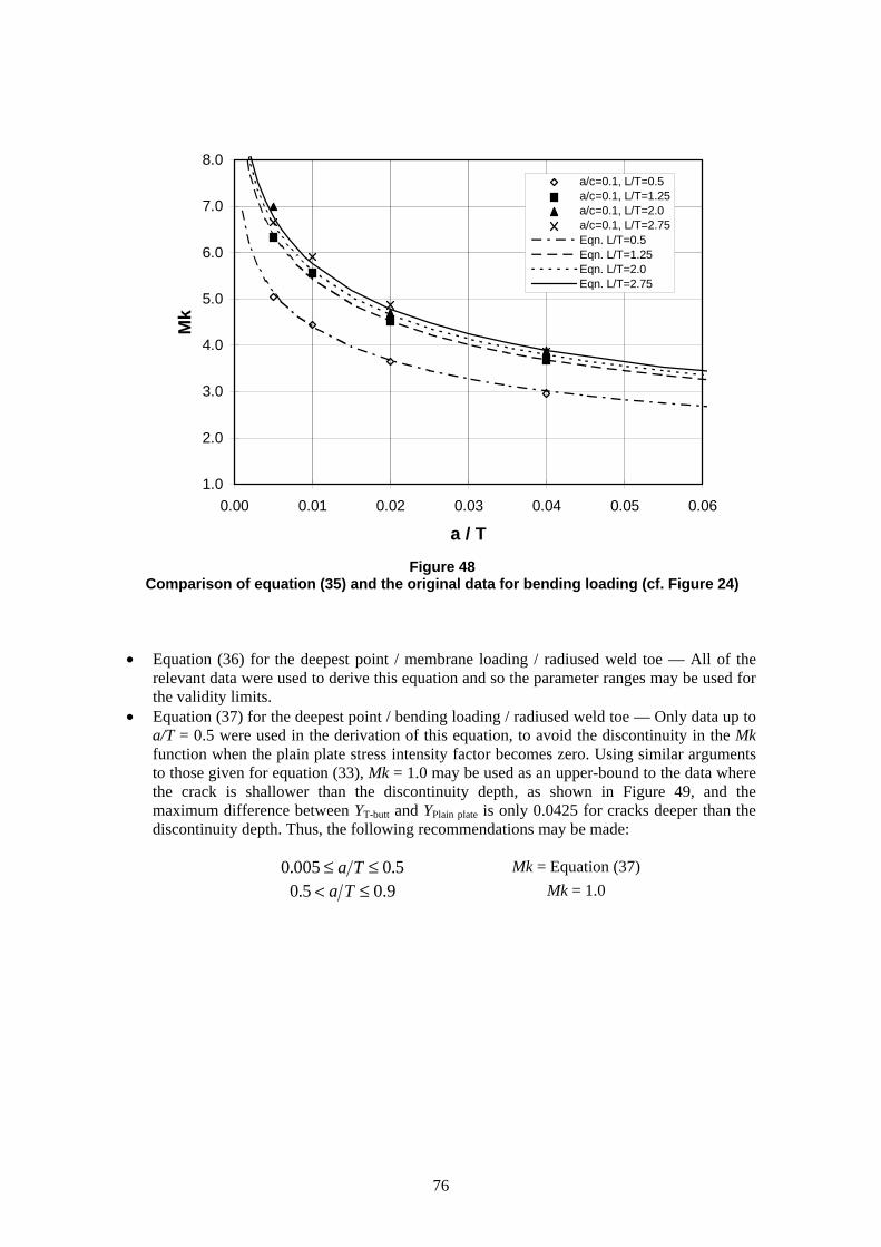
76

1.0

2.0

3.0

4.0

5.0

6.0

7.0

8.0

0.00 0.01 0.02 0.03 0.04 0.05 0.06

a / T

Mk

a/c=0.1, L/T=0.5a/c=0.1, L/T=1.25a/c=0.1, L/T=2.0a/c=0.1, L/T=2.75Eqn. L/T=0.5Eqn. L/T=1.25Eqn. L/T=2.0Eqn. L/T=2.75

Figure 48Comparison of equation (35) and the original data for bending loading (cf. Figure 24)

• Equation (36) for the deepest point / membrane loading / radiused weld toe — All of therelevant data were used to derive this equation and so the parameter ranges may be used forthe validity limits.

• Equation (37) for the deepest point / bending loading / radiused weld toe — Only data up toa/T = 0.5 were used in the derivation of this equation, to avoid the discontinuity in the Mkfunction when the plain plate stress intensity factor becomes zero. Using similar argumentsto those given for equation (33), Mk = 1.0 may be used as an upper-bound to the data wherethe crack is shallower than the discontinuity depth, as shown in Figure 49, and themaximum difference between YT-butt and YPlain plate is only 0.0425 for cracks deeper than thediscontinuity depth. Thus, the following recommendations may be made:

0 005 0 5. .≤ ≤a T Mk = Equation (37)

0 5. < ≤a T 0.9 Mk = 1.0

77

-3.0

-2.0

-1.0

0.0

1.0

2.0

0.4 0.5 0.6 0.7 0.8 0.9 1

a / T

Mk

Mk data before discontinuity

Upper bound line

Figure 49Mk data for bending loading, all L/T, a/c and 0 5. < ≤a T discontinuity depth

• Equation (38) for the crack ends / membrane loading / radiused weld toe — In thederivation of this equation, data for a/T = 0.005 were left out of the regression analysesbecause some of them showed a sudden drop with decreasing crack depth (see Section 6.3).If the equation is compared with all the relevant data in the database, the maximumoverprediction is 9.74% and the maximum underprediction is -5.12%. Therefore, theequation may be extended to the full parameter range without becoming unconservative.

• Equation (39) for the crack ends / bending loading / radiused weld toe — Similar toequation (38), the maximum overprediction of the equation compared to all the data is19.41% and the maximum underprediction is -3.27%. Hence, it is again possible to safelyextend the validity of the equation to the full parameter range.

8.2 OTHER VALIDITY LIMIT ISSUES

8.2.1 Extending the crack depth range

After the equations were regressed, a large number of graphs were plotted, for variouscombinations of the weld and crack parameters, to verify that the equations interpolated wellbetween the parameter values of the data in the database. During this verification, all graphswere plotted up to a depth of a/T = 1.0. These graphs revealed that the equations are stablebeyond their upper validity limit of a/T = 0.9, producing a smooth extrapolation of the crackdepth trends. An example of the extrapolated trends is shown in Figure 50. Hence, whilst theaccuracy of the equations is not certain beyond a/T = 0.9, they may be used to produce asensible extrapolation. The crack depth validity limit may, therefore, be tentatively stated asfollows:

0 005 1 0. .≤ <a T

78

0.0

0.5

1.0

1.5

2.0

2.5

3.0

0.5 0.6 0.7 0.8 0.9 1.0

a / T

Mk

Eqn. L/T=0.5

Eqn. L/T=1.25Eqn. L/T=2.0

Eqn. L/T=2.75

(a) deepest point

0.0

0.5

1.0

1.5

2.0

2.5

3.0

0.5 0.6 0.7 0.8 0.9 1.0

a / T

Mk

Eqn. L/T=0.5

Eqn. L/T=1.25Eqn. L/T=2.0

Eqn. L/T=2.75

(b) crack ends

Figure 50The extrapolated equation trends to a/T = 1.0, for a/c = 0.2

and θθ = 45° (membrane loading / sharp weld toe)

79

8.2.2 The weld angle for the radiused weld toe equations

In Section 5.4.3, the effect of the weld angle was demonstrated to be negligible when the weldtoe radius is 10% of the main plate thickness (ρ/T = 0.1). In the demonstration, weld angles

between 30° and 75° were used and so the equations should be valid for 30 75� �

≤ ≤θ . Tosignify the validity of the radiused weld toe equations for various weld angles, equations (36)–(39) may be multiplied by ( )f3 θ where ( )f3 1 0θ = . .

8.2.3 When should the sharp and radiused weld toe equations be used

The sharp weld toe equations are intended for use with ‘as-welded’ joints. The radiused weldtoe equations are intended for use with joints where the weld toe has been improved by localmachining or grinding, as specified in Section 21.2.13 c) ii) of the 3rd. Amendment of the 1995aHSE ‘Offshore Installations: Guidance on design, construction and certification’. They shouldnot be used otherwise, e.g. for the AWS Concave Improved Profile (ANSI / AWS Structuralwelding code, D1.1-90, 1990) where the general profile is concave but the weld toe is still ‘as-welded’. Of course, the radiused weld toe equations were derived for ρ/T = 0.1, and so theyshould not be used if the ground weld toe radius is smaller. Hence, for

0 0 0 1. .≤ <ρ T use the sharp weld toe equations

0 1. ≤ ρ T use the radiused weld toe equations

8.3 CONCLUSIONS ON THE VALIDITY OF THE EQUATIONS

The issues investigated in this section have been used to establish the validity limits of theequations. These limits and recommendations are stated concisely in Appendix B of this report,along with the final form of the new equations.

80

81

9. COMPARISONS WITH EXISTING Mk / SIF SOLUTIONS

In this section, the new weld toe magnification factor equations are compared with existingsolutions for both Mk and the SIF. The first comparison is with plain plate solutions to illustratethe effect of the weld toe magnification factors. The new equations are then compared with the2-D Mk factors from the current British Standards guidance (PD 6493, 1991), and the mostextensive set of 3-D Mk factors (Bell, 1987). Finally, the new equations are used in acomparison with the only existing parametric SIF equations for tubular joints (Rhee et al.,1991).

9.1 PLAIN PLATE SIF SOLUTIONS OF NEWMAN AND RAJU

The empirical SIF equation of Newman and Raju (1981) is a well established solution for asemi-elliptical surface crack in a plain plate, subjected to membrane and bending loading. Theequation, which is applicable to any location along the crack front, is included in PD 6493(1991).

The purpose of this comparison is to show the effect of a welded attachment on the shape factorY, where

YK

a=

σ π(41)

The comparison is shown in Figure 51 for the deepest point of the crack and Figure 52 for thecrack ends. In these Figures, the T-butt joint shape factors, for θ = 45° and L/T = 1.25, werecalculated from

MMkY .butt-T = (42)

where Mk is from the new equations for sharp weld toes (see Appendix B), and M is Newmanand Raju’s plain plate solution.

At the deepest point of the crack under membrane loading (Figure 51a), the welded attachmentis seen to increase the shape factor sharply for shallow cracks, which are under the influence ofthe weld toe notch stress. For intermediate crack depths (a/T from 0.2 to 0.9), the stiffeningeffect of the attachment reduces the shape factor below that of the plain plate. Beyond a/T = 0.9,the extrapolated new equations predict that the shape factor will again become more severe thanthat of the plain plate. For bending loading (Figure 51b), the trends for a/T < 0.5 are the same asfor membrane loading. However, beyond this crack depth, the shape factor for the T-butt jointjumps up to that for the plain plate, due to the conservative assumption made in Section 8.1, i.e.that Mk = 1.0 for a/T > 0.5.

At the crack ends for both membrane and bending loading (Figures 52a and b, respectively), theT-butt joint shape factor is always higher than that in the plain plate. This result is expectedbecause the crack end location is permanently influenced by the weld toe notch stress, though itseffect is greatest on shallow cracks.

82

0.0

0.5

1.0

1.5

2.0

2.5

3.0

3.5

4.0

4.5

0 0.2 0.4 0.6 0.8 1

a / T

YPlain plate

T-butt

a/c=0.1

a/c=1.0

a/c=0.4

a/c=0.2

(a) membrane loading

-0.5

0.0

0.5

1.0

1.5

2.0

2.5

3.0

0 0.2 0.4 0.6 0.8 1

a / T

Y

Plain plate

T-butt

a/c=0.1

a/c=0.2

a/c=0.4

a/c=1.0

(b) bending loading

Figure 51The effect of a welded attachment on the deepest pointshape factor, for θθ = 45° andL/T = 1.25 (sharp weld toe)

83

0.0

0.5

1.0

1.5

2.0

2.5

3.0

3.5

4.0

0 0.2 0.4 0.6 0.8 1

a / T

YPlain plate

T-butt

a/c=1.0

a/c=0.1

a/c=0.1

a/c=1.0

(a) membrane loading

0.0

0.5

1.0

1.5

2.0

2.5

3.0

3.5

4.0

0 0.2 0.4 0.6 0.8 1

a / T

Y

Plain plate

T-butt

a/c=0.1

a/c=0.1

a/c=1.0a/c=1.0

(b) bending loading

Figure 52The effect of a welded attachment on the crack end

shape factor, for θθ = 45° andL/T = 1.25 (sharp weld toe)

84

9.2 EDGE CRACK Mk FACTORS OF BS 7910

The weld toe magnification factors provided in BS 7910 (1997) which replaces PD 6493 (1991)were derived from 2-D plane strain slices of weld toe cracks, and so they are strictly only validfor edge cracks. Nevertheless, they are used here, along with the new equations, to compare theeffect of the attachment footprint width. For the comparison, shown in Figures 53a and b, formembrane and bending loading, respectively, a crack aspect ratio of 0.1 and a weld angle of 45°were used in the new equations.

The 2-D Mk factors are generally slightly higher than those from the new equations formembrane loading (Figure 53a), but this is reversed for bending loading (Figure 53b). Withregard to the effect of L/T, the general trends are the same for membrane loading but the 2-D Mkfactor solutions predict that the magnitude of the effect is larger. For bending loading, the 3-DMk factor solutions from the new equations predict a larger L/T effect than the 2-D Mksolutions, with the 2-D solutions predicting no extra effect when L/T is increased from 1.0 to2.75.

As well as the points noted in the above comparisons, there are two important differencesbetween the new solutions and the 2-D edge crack solutions of PD 6493. Firstly, for deepercracks (a/T > 0.3), the 2-D Mk factor solutions are unity since the 2-D T-butt joint behaves inexactly the same way as an edge cracked plate, which from Figure 6 is obviously not the casefor a semi-elliptical weld toe crack. Secondly, the 2-D solutions are not applicable at the crackends because they were derived from edge crack models. Despite this, the lack of full 3-D SIFsolutions has meant that 2-D solutions may be used to simulate 3-D T-butt joint crack endsolutions by applying the Mk for a very shallow crack, e.g. a = 0.15mm, to the plain plate crackend solutions (PD 6493, 1991). The use of a fixed small crack depth, however, yields a high Mkwhich is constant with crack depth, whereas Figure 7 shows that 3-D Mk factors exhibit a strongdependency on crack depth.

85

0.5

1.0

1.5

2.0

2.5

3.0

3.5

0.00 0.05 0.10 0.15 0.20

a / T

Mk

PD6493 L/T=0.5New Eqn. L/T=0.5PD6493 L/T=1.0New Eqn. L/T=1.0PD6493 L/T=2.75New Eqn. L/T=2.75

(a) membrane loading

0.5

1.0

1.5

2.0

2.5

3.0

0.00 0.05 0.10 0.15 0.20

a / T

Mk

PD6493 L/T=0.5New Eqn. L/T=0.5PD6493 L/T=1.0New Eqn. L/T=1.0PD6493 L/T=2.75New Eqn. L/T=2.75

(b) bending loading

Figure 53The effect of L/T on 2-D and 3-D Mk factor solutions, for a/c = 0.1 and θθ = 45°

(deepest point / sharp weld toe)

86

9.3 3-D T-BUTT JOINT Mk FACTORS OF BELL

The 3-D T-butt joint Mk factors of Bell (1987) were probably the most comprehensive set of 3-D weld toe magnification factors available, until recent times. Due to difficulties in fittingequations to the data, Bell presented the data in tabular form. The data are for a range of crackaspect ratios and weld angles, up to a crack depth ratio of a/T = 0.4, and are valid at the deepestpoint of the crack as well as the crack ends. In fact, the work of Bell was probably the first toshow that the weld toe magnification factor is not constant with crack depth at the crack endlocation, and also that it is not equal to the elastic stress concentration factor — anotherassumption allowed in PD 6493 (1991).

In Figures 54 and 55 for the deepest point and crack ends, respectively, the 3-D weld toemagnification factors of Bell, for θ = 45° are compared with those from the new equations. Inthese comparisons, the Mk factors from the new equations were calculated for a weld angle of45° and an attachment footprint width (L/T) of 2.0; Bell did not state the L/T used in his work,and so a value of 2.0 was estimated from his diagrams.

At the deepest point for the crack under membrane loading (Figure 54a), the trends are in verygood agreement, although the new equations predict a higher magnitude for a/T < 0.2. Forbending loading (Figure 54b), the agreement between the two sets of weld toe magnificationfactors is very good.

At the crack ends for both membrane and bending loading (Figures 55a and b, respectively), thegeneral trends with crack depth are in good agreement, but the new equations yield Mk factorsmuch higher than those of Bell. Also, the new equations show a distinct trend of increasing Mkwith decreasing a/c, whilst Bell’s results show no clear trends at all with a/c. The reasons for thedifferences at the crack ends is difficult to pin-point without a detailed knowledge of Bell’sfinite element meshes and analyses. But it is very likely, especially considering the fact that thework of Bell is over ten years old, that the meshes of Bell were much less refined than thoseused in this project, due to computing limitations at the time. Hence, Bell’s meshes wereprobably not refined enough to produce a converged solution in the region where the crack frontsingularity meets the weld toe singularity.

In Figure 56, the effect of the weld angle on the weld toe magnification factor is examined forbending loading. In this figure, the comparison is performed for a/c = 0.25 and L/T = 1.25; L/T= 1.25 was used in the new equations to remain within the validity limits when θ = 70°.

At the deepest of the crack (Figure 56a), the Mk factors from the new equations are slightlylower in magnitude than those of Bell. However, the trend with weld angle for shallow cracks(a/T < 0.1) is in very good agreement. At the crack ends (Figure 56b), the weld toemagnification factors of Bell are, again, very low, especially for the largest weld angle. The newequations also predict a noticeable trend with weld angle when the crack is 40% of the mainplate thickness in depth, whereas Bell’s data only shows a weld angle trend for a/T < 0.1.

87

0.8

1.0

1.2

1.4

1.6

1.8

2.0

0.0 0.1 0.2 0.3 0.4

a / T

Mk

Bell a/c=1.0New Eqn. a/c=1.0Bell a/c=0.5New Eqn. a/c=0.5Bell a/c=0.25New Eqn. a/c=0.25

(a) membrane loading

0.0

0.5

1.0

1.5

2.0

2.5

3.0

0.0 0.1 0.2 0.3 0.4

a / T

Mk

Bell a/c=1.0New Eqn. a/c=1.0Bell a/c=0.5New Eqn. a/c=0.5Bell a/c=0.25New Eqn. a/c=0.25

(b) bending loading

Figure 54Comparison with the 3-D Mk factors of Bell at the deepest point

of the crack, for θθ = 45° andL/T = 2.0 (sharp weld toe)

88

0.0

1.0

2.0

3.0

4.0

5.0

0.0 0.1 0.2 0.3 0.4

a / T

Mk

Bell a/c=1.0New Eqn. a/c=1.0Bell a/c=0.5New Eqn. a/c=0.5Bell a/c=0.25New Eqn. a/c=0.25

(a) membrane loading

0.0

1.0

2.0

3.0

4.0

5.0

6.0

0.0 0.1 0.2 0.3 0.4

a / T

Mk

Bell a/c=1.0New Eqn. a/c=1.0Bell a/c=0.5New Eqn. a/c=0.5Bell a/c=0.25New Eqn. a/c=0.25

(b) bending loading

Figure 55Comparison with the 3-D Mk factors of Bell at the crack

ends, for θθ = 45° andL/T = 2.0 (sharp weld toe)

89

0.6

0.8

1.0

1.2

1.4

1.6

1.8

0.0 0.1 0.2 0.3 0.4

a / T

Mk

Bell 30°New Eqn. 30°Bell 45 °New Eqn. 45°Bell 70 °New Eqn. 70°

(a) deepest point of the crack

0.0

1.0

2.0

3.0

4.0

5.0

6.0

0.0 0.1 0.2 0.3 0.4

a / T

Mk

Bell 30°New Eqn. 30°Bell 45 °New Eqn. 45°Bell 70 °New Eqn. 70°

(b) crack ends

Figure 56The effect of weld angle on the weld toe magnification factor under

bending loading, for a/c = 0.25 and L/T = 1.25 (sharp weld toe)

90

9.4 3-D T-BUTT JOINT SIF SOLUTIONS OF BRENNAN ET AL.

In this report, it was hoped that the new equations could be compared with the 3-D T-butt jointSIF solutions of Brennan et al. (To be published). These solutions are based on Niu andGlinka’s weight function for the deepest point of the crack, and Shen and Glinka’s weightfunction at the surface point (crack ends). The data derived by Brennan et al. were regressedinto equation form by C. Arbuthnot and Associates (1998).

Despite coding the equations very carefully into FORTRAN, and checking them several times,it was not possible to get realistic SIF values from the four equations. Problems with thesesolutions have been noted elsewhere (BS 7910 Draft, 1997), and so no comparison is includedin this report due to the fact that the equations appear to be unreliable.

9.5 TUBULAR T-JOINT SIF SOLUTIONS OF RHEE ET AL.

The SIF solutions of Rhee et al. (1991) are the only parametric SIF equations for tubular joints.They were derived from three-dimensional finite element analyses of semi-elliptical saddlecracks in tubular T-joints, and are applicable to axial as well as in- and out-of-plane bendingloading. Equations are provided for the deepest point of the crack and the crack ends.

In this section, the new equations are used to predict tubular joint shape factors (Y), which arethen compared with those from Rhee et al.’s parametric formulae. The geometry of the tubularT-joint chosen for comparison is as follows:

T = 32mmβ = d/D = 0.5τ = t/T = 0.5γ = D/2T = 14.29

which lies well within the validity ranges of Rhee et al.’s equations. The predicted shape factorsfrom the new equations were calculated from

( ) DOBSCFMMkDOBSCFMMkY bbmm .1 +−= (43)

where Mk is the weld toe magnification factor from the new equations, M the plain plate shapefactor from Newman and Raju (1981) and the SCF and DOB (stress concentration factor anddegree of bending, respectively) describe the uncracked stress field at the location of the crack.For the T-joint chosen, the SCF and DOB at the saddle were found, from previous workconducted at Swansea (Bowness, 1996), to be

Axial brace loading SCF = 6.58 DOB = 0.792Out-of-plane bending SCF = 5.07 DOB = 0.832

With regard to the geometry of the weld, the weld angle in the new equations was assumed to be45°, and L/T was calculated from the AWS D1.1-90 (1990) recommendations for a standard flatweld profile as 0.674 (see Tables 1 and 2).

To calculate shape factors from the equations of Rhee et al., one must first consider the validitylimits of their equations:

0 05 0 8. .≤ ≤a T0 05 3 1 2. .≤ ≤c d

91

Whilst the crack depth validity limits are given in a conventional form, the crack width has beennon-dimensionalised by the brace diameter. By using the tubular joint geometric ratios, it ispossible to express the crack width validity limits in terms of the more conventional parametera/c:

( )( )0 05

3

21 2. .≤ ≤

a T

a cβγ

Hence, for β = 0.5 and γ = 14.29, it follows that the crack aspect ratio validity limits of Rhee etal.’s equations are

( )0 175 4 2. .a

Ta c

a

T

≤ ≤

These validity limits are plotted in Figure 57 up to a crack aspect ratio of a/c = 1.0. The validitylimits extend from very wide cracks at shallow depths to more rounded cracks (higher a/c) atdeeper depths, though it should be noted that rounded cracks (high a/c) will only exist forshallow crack depths, and the high bending stresses in tubular joints results in wide cracks athigh a/T. The equations are valid up to a/c = 3.36 at a/T = 0.8.

The importance of carefully checking the validity limits of the equations of Rhee et al. isillustrated in Figure 58, which shows the effect of a/c on the shape factors, at the deepest pointof a crack, in an axially loaded T-joint. The curve for a/c = 1.0 shows that this equation can behighly unstable for cracks shallower than a/T of 0.1. Initially, one might think that the shapefactor curves in the figure are within the crack depth validity limits (a/T between 0.05 and 0.8),but because the a/c limits are also functions of a/T, they have actually been extrapolated beyondtheir limits.

Having established the validity limits, shape factors calculated using the equations of Rhee et al.are compared with those predicted from the new equations in Figures 59 and 60, for axialloading and out-of-plane bending, respectively.

92

0.0

0.2

0.4

0.6

0.8

1.0

0 0.1 0.2 0.3 0.4 0.5 0.6 0.7 0.8

a / T

a / c

Upper validity limit

Lower validity limit

Figure 57Crack aspect ratio validity limits of Rhee et al.’s

parametric formulae, for ββ = 0.5 and γγ = 14.29

0

20

40

60

80

100

120

0.0 0.1 0.2 0.3 0.4 0.5 0.6 0.7 0.8

a / T

Y

Rhee a/c=0.1Rhee a/c=0.2Rhee a/c=0.4Rhee a/c=1.0

Figure 58Effect of a/c on an axially loaded tubular T-joint, for ββ = 0.5, ττ = 0.5 and γγ = 14.29 (deepest

point). Note that the validity limits of the equation have been exceeded.

93

At the deepest point of the crack in the axially loaded T-joint (Figure 59a), the generalagreement is quite good, especially for deeper cracks (a/T > 0.4). For the two widest cracks (a/c= 0.1 and 0.2), the new equations predict lower shape factors than Rhee et al.’s equations for a/Tof between 0.1 and 0.3, but for crack depths shallower than this, the new equations begin toincrease sharply to values close to those of Rhee et al.. At the crack ends (Figure 59b), theagreement between the two sets of solutions is poor except, perhaps, for the a/c = 0.2 curve.

To try to account for the poor agreement between the solutions at the crack ends, the data fromwhich Rhee et al. derived their parametric formulae must be examined. Rhee et al. used thedisplacements of the quarterpoint nodes to calculate their SIFs. Since several elementssurrounded the crack tip, they calculated several SIFs for every point along the crack front, onefor each radial line of nodes. Along most of the crack front, the SIFs from different radial lineswere in good agreement, but they observed a large scatter in SIF values where the crack frontmeets the weld toe. Rhee (1989) attributed this variation to modelling difficulties stating that‘solutions evaluated from different crack tip radial lines at a crack tip point should be identical ifthe finite element solutions are exact’. Thus, their equations for the crack ends were regressedfrom data where ‘the inside solutions were extrapolated, guided by the data distribution at thelocation, to obtain the respective SIF solution’ (Rhee et al., 1991). However, the SIF distributionrises sharply as the crack ends are approached, because of the weld toe notch stress. Hence,there may be an error in the extrapolation. Also, their statement regarding the agreement ofsolutions from different radial lines is not strictly correct because the geometry is unsymmetric,and so the displacements of the radial lines, and the associated SIFs, will be less on the weldside of the crack. Their SIFs at this location are, therefore, subject to uncertainty.

For the out-of-plane bending loaded T-joint (Figure 60), the results of the comparison are thesame as for the axially loaded T-joint.

94

0

1

2

3

4

5

6

7

8

9

0 0.1 0.2 0.3 0.4 0.5 0.6 0.7 0.8a / T

Y

Rhee a/c=0.1New Eqns. a/c=0.1Rhee a/c=0.2New Eqns. a/c=0.2Rhee a/c=0.4New Eqns. a/c=0.4Rhee a/c=1.0New Eqns. a/c=1.0

(a) deepest point

3

4

5

6

7

8

9

10

11

0 0.1 0.2 0.3 0.4 0.5 0.6 0.7 0.8a / T

Y

Rhee a/c=0.1New Eqns. a/c=0.1Rhee a/c=0.2New Eqns. a/c=0.2Rhee a/c=0.4New Eqns. a/c=0.4Rhee a/c=1.0New Eqns. a/c=1.0

(b) crack ends

Figure 59Comparison of shape factors for an axially loaded

tubular T-joint, for ββ = 0.5, ττ = 0.5 and γγ = 14.29 (sharp weld toe)

95

0

1

2

3

4

5

6

7

0 0.1 0.2 0.3 0.4 0.5 0.6 0.7 0.8a / T

Y

Rhee a/c=0.1New Eqns. a/c=0.1Rhee a/c=0.2New Eqns. a/c=0.2Rhee a/c=0.4New Eqns. a/c=0.4Rhee a/c=1.0New Eqns. a/c=1.0

(a) deepest point

2

3

4

5

6

7

8

9

0 0.1 0.2 0.3 0.4 0.5 0.6 0.7 0.8a / T

Y

Rhee a/c=0.1New Eqns. a/c=0.1Rhee a/c=0.2New Eqns. a/c=0.2Rhee a/c=0.4New Eqns. a/c=0.4Rhee a/c=1.0New Eqns. a/c=1.0

(b) crack ends

Figure 60Comparison of shape factors for an out-of-plane bending loadedtubular T-joint, for ββ = 0.5, ττ = 0.5 and γγ = 14.29 (sharp weld toe)

96

97

10. COMPARISONS WITH TUBULAR JOINT SIFs

The purpose of the work presented in this section is to demonstrate that the new T-butt joint SIFsolutions may be reliably used to calculate tubular joint SIFs. To this end, a modellingprocedure for uncracked and cracked tubular joints is first described and then used to evaluatetubular joint stress fields and stress intensity factors — the stress field data are used as input tocalculate SIFs from the T-butt joint solutions, which are compared with the numerical tubularjoint values. Also, the relative merits of linear and quadratic extrapolation for the evaluation ofthe uncracked geometric stress field are investigated.

10.1 NUMERICAL MODELLING OF CRACKED TUBULAR JOINTS

10.1.1 Mesh generation for a basic quarter T-joint

The starting block for the mesh generation of the most basic of tubular joint geometries — aquarter T-joint mesh, i.e. utilising two planes of symmetry — is a T-butt joint mesh (thegeneration of T-butt joint models is described in Section 2.1). The FORTRAN programABAMAP, which was developed at Swansea (Bowness, 1996), performs a series of mappingson a 3-D T-butt joint to produce the T-joint mesh. The sequence of mappings is shown in Figure61.

The diameter of the chord is determined by the length of the main plate; by adjusting this lengthand the relative position of the attachment (Figure 61a), T-joint models with different chorddiameters and β ratios may be produced. To turn the T-butt joint into a tubular joint, it is firstcurved around 90º such that the attachment forms a brace (Figure 61b). The main plate, now aquarter circle, is then mapped into a square (Figure 61c), which when curved around 90º forms asegment of the top of the chord (Figure 61d). Finally, the rest of the chord is added resulting in aquarter tubular T-joint mesh (Figure 61e). The resulting model has refined crack front and weldtoe meshes, and has adjustable α, τ, β and γ ratios as well as the weld angle and toe radius. Inputparameters also allow meshes with different portions of the chord circumference to begenerated. For example, the mesh in Figure 61d models a quarter of the chord circumference,but for certain joints only an eighth of the circumference is needed (see the following section).

The resulting mesh from the program ABAMAP contains a semi-elliptical crack located at thesaddle of the joint. For certain loadings, however, the hot spot stress occurs at the crown and sothe program FLIPMAP must be used. This program initially flips the T-butt joint mesh such thatthe left and the right are swapped, i.e. the crack ends up on the other side of the mesh, and thenperforms exactly the same mappings as ABAMAP, resulting in a quarter T-joint with a crowncrack.

10.1.2 Mesh generation of more complex joints

All of the other joints modelled in this work began life as quarter T-joints and were then built upthrough a series of mappings, reflections and rotations to the basic model. This technique isillustrated in Figure 62, where the generation of a T-joint with an out-of-plane brace is shown.

One of the two braces is formed by adding together two quarter T-joint meshes – one of themeshes has an eighth of the chord circumference, whilst the other has one quarter. The chordlength and a further eighth of its circumference are then added to result in a quarter of the

98

desired mesh, with half of one brace and two planes of symmetry. Finally, two of these meshesmay be joined to form the final mesh which utilises one plane of symmetry.

For angled braces such as Y- and K-joints, the FORTRAN program YBRACE may be used tomap the brace of a T-joint to the required angle, as shown in Figure 63.

The final consideration when generating models of more complex joints is the location of thecrack. Because the joints start out as quarter T-joints, a crack mesh always exists at every saddle(or crown). Thus, in the case of the T-joint with an out-of-plane brace (Figure 62d), there arefour cracks – one at each saddle. To alleviate this problem, the unwanted cracks may beremoved from the model by merging the nodes on the crack faces, leaving one crack in thedesired location. Also, for uncracked analyses, all of the cracks may be closed up in a similarmanner.

10.1.3 Analysis

The element type chosen for the analyses was the reduced integration 20-noded brick C3D20Rfrom the ABAQUS (1997) element library. As with the T-butt joint meshes (Section 2.2), thecrack front elements are collapsed bricks with the midside nodes remaining at the halfwaypoints.

The loadings on the models obviously varied with the joint configuration and the loading mode(details of which follow later). In all cases, the chord end was fixed (encastre) and loadings wereachieved via applied displacements. Symmetry and, in some cases, antisymmetry conditionswere used as appropriate.

The Young’s modulus and the Poisson’s ratio used in the analyses were 210 kNmm-2 and 0.3,respectively. The elastic finite element calculations were performed using the general purposefinite element package ABAQUS (1997). The size of the tubular joint models varies enormously– the largest model analysed was a half multiplanar K-joint (K with an out-of-plane K) whichcontained 28,000 brick elements and 400,000 degrees of freedom; the cpu time required to solvethis model was just over 3 hours on a Sun Ultra 2170.

99

(a) adjust main plate length to produce a joint with the desired β ratio

(b) curve the T-butt jointaround 90º so that the

attachment becomes thebrace

(c) make the main plate square

Figure 61ABAMAP modelling sequence (cont’d overleaf)

100

(d) curve the main platearound 90º to form the chord

Figure 61ABAMAP modelling sequence (continued)

(e) add the rest of the chord tocreate a quarter T-joint

101

(a) A mesh with half the brace may beformed by joining together two quarter T-joint meshes – one with an eighth of thechord circumference and the other with a

quarter

(b) The rest of the chord may be added tothe mesh from part (a) to yield a half bracemesh with half of the chord circumference

Figure 62Sequence for generating a T-joint with an out-of-plane brace (cont’d overleaf)

102

(c) Join two meshes from part (b) together

(d) The resulting mesh

Figure 62Sequence for generating a T-joint with an out-of-plane brace (continued)

103

(a) The initial T-joint

(b) The mapped brace

Figure 63Mapping a brace to an angle

10.1.4 Calculation of SIFs and the shape factor Y

In the T-butt joint parametric study (Sections 3 and 5.2), the J-integral, obtained via the virtualcrack extension, was used to provide reliable estimates of the crack front stress intensity factors.For the tubular joint models, the same method was used with plane strain conditions assumedeverywhere along the crack front when calculating the SIFs.

To non-dimensionalise the SIFs into shape factors (Y), it is necessary to calculate a nominalstress such that Y is independent of the loading magnitude. When the joint is axially loaded, thenominal stress was taken to be the average stress in the reference brace:

AFnom =σ (44)

where F is the reaction force at the end of the brace and A is the brace cross-sectional area. Forin- and out-of-plane bending loading, the nominal stress was taken as the extreme fibre stress:

104

−−

π

=σ44

22

2

tdd

Fldnom (45)

where F is the reaction force at the end of the brace, l the distance between the brace end andthe crown, d the brace diameter and t the brace wall thickness. For joints with an angled brace,the lever arm l was calculated as the average distance between the brace end and the crown heeland toe. Note that for multi-braced axially loaded joints, the reference brace in this work is thetensile brace, unless otherwise specified.

10.2 PREDICTION OF TUBULAR JOINT SIFs FROM T-BUTT JOINT SOLUTIONS

10.2.1 Approximation of tubular joint SIFs

The general equation for calculating T-butt joint SIFs is

[ ] aMMkMMkK bbbmmm πσ+σ= (46)

where a is the crack depth, Mk the weld toe magnification factors, M the plain plate shapefactors, σ the nominal plate stresses, and m and b denote membrane and bending loading,respectively. Note that in this work, the plain plate correction factors of Newman and Raju(1981) are used. To approximate tubular joint SIFs from T-butt joint solutions, equation (46)may be written in the following form:

( )[ ] aDOBSCFMMkDOBSCFMMkK nombbmm πσ+−≈ .1jointtubular (47)

where SCF is the stress concentration factor and DOB the degree of bending at the would-belocation of the crack, and σnom is the nominal stress in the reference brace of the joint; all thesequantities are for the uncracked tubular joint. In this equation,

( )[ ] YDOBSCFMMkDOBSCFMMk bbmm =+− .1 (48)

where Y is the predicted tubular joint shape factor (non-dimensional SIF). The SCF in equations(47) and (48) must be derived from the geometric hot spot stress, which incorporates the effectsof the overall tube geometry and joint configuration but omits the stress concentrating influenceof the weld geometry. This is necessary because the influence of the weld geometry is alreadyincorporated into the weld toe magnification factors.

10.2.2 Calculation of the SCF

In the HSE design guidance (1995a), stress-endurance fatigue design is based on the geometrichot spot stress calculated by the extrapolation, to the weld toe, of the geometric stressdistribution near the weld toe, as shown in Figure 64. Such a geometric hot spot stress isconsistent with the requirements stated in the previous section.

105

Figure 64The geometric hot spot stress (HSS)

Guidance on how the extrapolation should be performed, which was formulated from large scaletest results from the ECSC and UKOSRP research programmes, is given in the BackgroundNotes to the original Department of Energy Guidance (1984). For T-butt joints, it was noted thatthe stress distribution along the main plate is linear apart from near to the weld toe, where thedistribution is disturbed and rises rapidly. The research programmes found that a linear region isalso present in some geometries of T- and X-joints, which lead to the guidance that the hot spotstress should be evaluated by extrapolating this linear region to the weld toe. In particular, theguidance conservatively recommends the extrapolation of the maximum principal stress ratherthan the stress component perpendicular to the weld toe. Figure 65 summarises the extrapolationrecommendations, where B1-4 denote the extent of the influence of the weld toe, A1-4 the extentof the linear region, r is the brace radius and R the chord radius.

106

Figure 65The regions of stress linearity from the Background to

the Department of Energy Guidance (1984)

In this work, a Linear SCF was determined in accordance with the above recommendations.That is, the geometric weld toe stress was obtained by extrapolating the maximum principalstress distribution, in the region given by Figure 65, to the weld toe, and then non-dimensionalising the result by the nominal brace stress.

It is noted in the Background to the Department of Energy Guidance (1984) that not all tubularjoint geometries and configurations have a region of stress linearity, especially in Y- and K-joints. Consequently, some researchers have used non-linear extrapolation with a third straingauge rosette positioned equidistant from the second gauge, i.e. further away from the weld toethan point A in the figure and spaced the same distance from A as B (Smedley and Fisher, 1991).Also, it is possible that the extent of the influence of the weld toe does not coincide with thebeginning of the region of stress linearity. Figure 5, in Section 3, shows the stress distribution inT-butt joints with various attachment footprint widths, and from this figure it may be seen thatthe influence of the weld toe extends to about 0.25T from the toe. Figure 66 shows the chordside stress distribution at the saddle of an uncracked tubular T-joint (α = 14, β = 0.5, γ = 18, τ =0.6, T = 1, d = 18, D = 36). The data points plotted in this figure show a slight oscillationbetween corner and midside node values due to the high stress gradient. In part (a), thedistribution has been linearly extrapolated in accordance with the Background to theDepartment of Energy Guidance; from Figure 65, A4/T = 1.571 and B4/T = 0.465. In part (b), aquadratic extrapolation is shown which extends from a third point equidistant from A4, i.e. at2A4/T–B4/T = 2.677, to 0.25.

107

0

5

10

15

20

25

30

35

0.0 0.5 1.0 1.5 2.0 2.5 3.0

Distance from weld toe / T

SC

FNodal FE dataExtrapolation dataLinear extrapolation

(a) linear extrapolation (SCF = 10.71)

0

5

10

15

20

25

30

35

0.0 0.5 1.0 1.5 2.0 2.5 3.0

Distance from weld toe / T

SC

F

Nodal FE dataExtrapolation dataQuadratic extrapolation

(b) quadratic extrapolation (SCF = 12.16)

Figure 66Chord side stress distribution at the saddle of a tubular T-joint

(αα = 14, ββ = 0.5, γγ = 18, ττ = 0.6, T = 1, d = 18, D = 36)

108

From Figure 66a, the Background to the Department of Energy Guidance does indicate a regionof stress linearity. However, the quadratic extrapolation, shown in part (b), appears to be a betteroverall fit to the stress distribution. Also, because the distribution is a good fit up to andincluding the data point at 0.25T (the extent of the notch stress in T-butt joints), the extent of theinfluence of the weld toe in tubular joints must be less than that given in Figure 65. For thisparticular geometry, the quadratic SCF is 13% higher than that obtained linearly, which is morethan double the 5% maximum difference noted in previous work (Smedley and Fisher, 1991).But in previous work, the extrapolation was performed up to the end of the linear region whichmay well yield an unconservative estimate of the actual geometric stress. Hence, quadraticextrapolation is likely to give a more accurate estimate of the geometric stress at the weld toeand, thus, better SIFs. For this reason, as well as computing SIFs using a linearly extrapolatedSCF, calculations in this work will also be carried out using a Quadratic SCF, obtained byextrapolating from a point equidistant from the two locations given in Figure 65 to 0.25T.

10.2.3 Calculation of the DOB

The degree of bending is defined as

−=

σσ=

outer

inner12

1

SCF

SCFDOB

t

b (49)

where σb is the bending stress, σt the total stress (= SCF × σnom), SCFinner the geometric SCF onthe inner surface of the chord under the weld toe and SCFouter the geometric SCF at the weld toe(= SCF as discussed in the previous section). Unlike at the weld toe, the stress distribution onthe inner surface of the chord is not subject to a rapidly increasing stress gradient, as shown inFigure 67. Some disturbance due to the weld toe effect will occur because of the need for thecross-section to self equilibrate, but this is difficult to quantify and is likely to be negligible.Thus, in this work, SCFinner is taken to be the averaged nodal stress at the node on the innersurface directly under the weld toe. Even though SCFinner is the same no matter how the SCF atthe weld toe is evaluated, for each uncracked joint geometry and configuration, two DOBs mustbe calculated from equation (49): one corresponding to the linear SCF and the other thequadratic SCF.

109

-10

-8

-6

-4

-2

0

-2.0 -1.5 -1.0 -0.5 0.0 0.5 1.0 1.5 2.0

Distance from weld toe / T

SC

F

Figure 67Chord inner surface stress distribution at the saddle of a tubular T-joint

(αα = 14, ββ = 0.5, γγ = 18, ττ = 0.6, T = 1, d = 18, D = 36)

10.2.4 Application of the SIF equation

As well as considering how the uncracked stress field parameters should be evaluated, becausethe stress field changes around the intersection of tubular joints, one must also consider thestresses to be used when applying the SIF equation. The simplest way to evaluate equation (47)is to use the SCF and DOB corresponding to the location of the deepest point of the crack, forboth the deepest point and the crack ends. Usually, the crack will be centred on the hot spotlocation and so the hot spot SCF and DOB will be used. As the crack widens, however, thecrack ends may have moved a considerable distance from the hot spot. This has lead to someresearchers advocating the use of the intersection stress distribution to calculate a local SCF andDOB corresponding to the actual location of the crack ends (Thurlbeck, 1991). Also, in somemethodologies, the change in the geometry of the weld around the intersection is taken intoaccount (Thurlbeck, 1991).

In this work, most SIFs are calculated by using the SCF and DOB corresponding to the centre ofthe crack, which is usually at the hot spot of the joint. And for some joints, the use of a localSCF and DOB, derived from the intersection stress distribution, is investigated.

110

10.3 CORRELATION BETWEEN TUBULAR JOINT AND T-BUTT JOINT SIFs

10.3.1 Configurations and geometries of joints studied

Details of the tubular joint analyses performed for the comparison are given in Table 8. Thejoints analysed were chosen to encompass a wide range of configurations, geometries andloadings. In the table, the geometries are described in terms of the standard tubular joint non-dimensional parameters as defined in Figure 68 (angles are given in degrees), and the weldgeometry is that at the location of the centre of the crack; crack locations are given in Table 9.In total, 26 uncracked and 95 cracked tubular joints were analysed.

� � � � �� � � � �

�

� �

� � �

�

�

�

�

� � �� � �

� � � � �

! " # $ %

& ' ( ) * +

, - . / 01 2 3 3 4 5

6 7 7 8 9 : ;

d = brace diameter D = chord diametert = brace wall thickness T = chord wall thicknessθ = angle of brace / chord intersection g = gap (distance between brace toes)L = chord length (distance between end

restraints)e = joint eccentricity

α = 2L / D β = d / Dγ = D / 2T τ = t / Tζ = g / D φ = out-of-plane brace angle

Figure 68Geometric notation for tubular joints

Typical meshes for each joint configuration and the loadings applied are shown in Figures 69–76. Also, Figure 77 shows a deformed mesh plot, including a close-up of the opened crack, forthe T-joint with an out-of-plane T.

Tab

le 8

Par

amet

erm

atri

xfo

rth

eu

ncr

acke

dan

dcr

acke

dtu

bu

lar

join

tan

alys

es(o

op

=o

ut-

of-

pla

ne)

No

teth

atal

l jo

ints

are

co

nce

ntr

ic, i

.e.t

he

ecce

ntr

icit

y=

0

� ����� ��

� �� �� �

�

� �� � �

� �� �� ��� �� � �

����� ��

� �� ���� �

� ���� �� ��

� ��� ���

� ��� ����

�� �� � �� �

� ���

� �����

!"� � �!#�$

ααββ

γγττ

θθζζ

φφ

�%�

θθ

�%�

�% �

� ���� � & �

���� �

T1

TA

xial

tens

ion

140.

518

0.6

90—

—0.

9343

0.01

,0.0

4,0.

1,0.

3,0.

5,0.

70.

1,0.

4,1.

018

1T

1T

Axi

al te

nsio

n14

0.5

180.

690

——

0.93

430.

90.

11

0T

2T

Axi

al te

nsio

n14

0.3

180.

690

——

0.86

640.

01,0

.1,0

.50.

43

1T

3T

Axi

al te

nsio

n14

0.7

180.

690

——

1.17

300.

01,0

.1,0

.50.

43

1T

4T

Axi

al te

nsio

n14

0.5

80.

690

——

0.92

430.

01,0

.1,0

.50.

43

1T

5T

Axi

al te

nsio

n14

0.5

260.

690

——

0.93

430.

01,0

.1,0

.50.

43

1T

6T

Axi

al te

nsio

n14

0.5

180.

490

——

0.62

430.

01,0

.1,0

.50.

43

1T

7T

Axi

al te

nsio

n14

0.5

180.

890

——

1.23

430.

01,0

.1,0

.50.

43

1T

8T

Axi

al te

nsio

n14

0.5

181

90—

—1.

5443

0.01

,0.1

,0.5

0.4

31

T9

TIP

B14

0.5

180.

690

——

0.90

550.

01,0

.1,0

.50.

43

1T

10T

OPB

140.

518

0.6

90—

—0.

9343

0.01

,0.1

,0.5

0.4

31

DT

1D

TA

xial

tens

ion

140.

718

0.6

90—

—1.

1730

0.01

,0.1

,0.5

0.4

31

TT

1T

with

oop

TB

oth

brac

este

n.14

0.5

180.

690

—90

1.03

330.

01,0

.1,0

.50.

43

1T

T2

Tw

ith

oop

T1

ten.

,1co

mp.

140.

518

0.6

90—

901.

0333

0.01

,0.1

,0.5

0.4

31

DT

T1

DT

with

oop

TA

llbr

aces

tens

ion

140.

518

190

—90

1.54

430.

01,0

.1,0

.50.

43

1D

TT

2D

Tw

ithoo

pT

DT

ten.

,oop

bra

ce c

omp.

140.

518

190

—90

1.54

430.

01,0

.1,0

.50.

43

1

Y1

YA

xial

tens

ion

140.

518

0.6

60—

—0.

9343

0.01

,0.0

41.

02

1Y

1Y

Axi

al te

nsio

n14

0.5

180.

660

——

0.93

430.

1,0.

30.

42

0Y

1Y

Axi

al te

nsio

n14

0.5

180.

660

——

0.93

430.

5,0.

70.

12

0

K1

KB

alan

ced

axia

l16

0.5

80.

645

-45

0.29

—1.

1334

0.01

,0.1

,0.5

0.4

31

K2

KIP

Bop

enin

gm

omen

ts16

0.5

80.

645

-45

0.29

—1.

1334

0.01

,0.1

,0.5

0.4

31

K3

KB

alan

ced

axia

l14

0.5

180.

445

-45

0.29

—0.

7634

0.01

,0.1

,0.5

0.4

31

K4

KIP

Bop

enin

gm

omen

ts14

0.5

180.

445

-45

0.29

—0.

7634

0.01

,0.1

,0.5

0.4

31

DK

1D

KS

ymm

.bal

.ax.

160.

58

0.6

45-4

50.

29—

1.13

340.

01,0

.1,0

.50.

43

1D

K2

DK

Ant

isym

m.b

al.a

x.16

0.5

80.

645

-45

0.29

—1.

1334

0.01

,0.1

,0.5

0.4

31

DK

3D

KS

ymm

.bal

.ax.

140.

518

0.4

45-4

50.

29—

0.76

340.

01,0

.1,0

.50.

43

1D

K4

DK

Ant

isym

m.b

al.a

x.14

0.5

180.

445

-45

0.29

—0.

7634

0.01

,0.1

,0.5

0.4

31

KK

1K

wit

hoo

pK

Sym

m.b

al.a

x.14

0.5

180.

445

-45

0.29

900.

7634

0.1,

0.5

0.4

21

KK

2K

wit

hoo

pK

Ant

isym

m.b

al.a

x.14

0.5

180.

445

-45

0.29

900.

7634

0.1,

0.5

0.4

21

TO

TA

L95

26

112

(a) typical mesh (axial loading)

Axial In-plane-bending (IPB) Out-of-plane bending (OPB)

(b) loadings corresponding to the applied displacements

Figure 69A typical T-joint mesh and the loadings applied

Axial loading: Quarter model - two planes of symmetryBending loadings: Half model - one plane of symmetry

113

(a) typical mesh

Axial

(b) loading corresponding to the applied displacement

Figure 70A typical DT-joint mesh and the loading applied

Axial loading: Eighth model - three planes of symmetry

114

(a) typical mesh

Both braces tension One brace tension, the other compression

(b) loadings corresponding to the applied displacements

Figure 71A typical T-joint with an out-of-plane T mesh and the loadings applied

Both loadings: Half model - one plane of symmetry

115

(a) typical mesh

All braces tension DT braces tension, the out-of-plane bracecompression

(b) loadings corresponding to the applied displacements

Figure 72A typical DT-joint with an out-of-plane T mesh and the loadings applied

Both loadings: Quarter model - two planes of symmetry(reference braces are those that form the DT)

116

(a) typical mesh

Axial

(b) loading corresponding to the applied displacement

Figure 73A typical Y-joint mesh and the loading applied

Axial loading: Half model - one plane of symmetry

117

(a) typical mesh

Balanced axial In-plane bending opening moments

(b) loadings corresponding to the applied displacements

Figure 74A typical K-joint mesh and the loadings applied

Both loadings: Half model - one plane of symmetry

118

(a) typical mesh

Symmetrical balanced axial Antisymmetrical balanced axial

(b) loadings corresponding to the applied displacements

Figure 75A typical DK-joint mesh and the loadings applied

Symmetrical balanced axial loading: Quarter model - two planes of symmetryAntisymmetrical bal. ax. loading: Quarter model - one symmetry and one antisymmetry plane

119

(a) typical mesh

Symmetrical balanced axial Antisymmetrical balanced axial

(b) loadings corresponding to the applied displacements

Figure 76A typical K-joint with an out-of-plane K mesh and the loadings applied

Symmetrical balanced axial loading: Half model - one plane of symmetryAntisymmetrical bal. ax. loading: Half model - one plane of antisymmetry

120

(a) deformed mesh plot

(b) close-up of the crack opening

Figure 77Deformed mesh plot of geometry TT1 with an a/T = 0.5, a/c = 0.4 crack

121

10.3.2 Uncracked stress field results

The uncracked stress field results are given in Table 9. For all of the joints, with the exceptionof TT1, the stress field is that at the hot spot, which was also the location of the crack in thecracked joint analyses. For joint TT1, the crack was not located at the hot spot and so the stressfield at the hot spot and the crack location are given. The SCFs and DOBs calculated fromparametric equations are those of Efthymiou (1988) and Connolly et al. (1990), respectively.

Comparing extrapolation methods, it can be seen that the quadratic SCF is between 6 and 24%higher than that obtained by linear extrapolation, with an average increase of 11%. As regard tothe parametric SCF equations, there is reasonable agreement with the equations, overpredictingthe linear SCF by between 1 and 29%. The DOB equations give better predictions, ranging from–3 to +6% when compared to the linear DOB.

Tab

le 9

Un

crac

ked

stre

ssfi

eld

resu

lts

(in

ner

/ou

ter

sad

dle

den

ote

sth

ete

nsi

on

bra

cesa

dd

len

eare

st t

o/f

urt

hes

t fr

om

the

adja

cen

tb

race

)

Geo

met

ryH

ot

spo

to

rcr

ack

Qu

adra

tic

extr

apo

lati

on

Lin

ear

extr

apo

lati

on

Par

amet

ric

equ

atio

ns

Qu

ad/L

in&

load

Ref

.lo

cati

on

ifd

iffe

ren

tS

CF

DO

BS

CF

DO

BS

CF

DO

BS

CF

T1

HS

(sad

dle)

12.2

0.81

10.7

0.86

11.4

0.84

1.14

T2

HS

(sad

dle)

10.8

0.81

9.79

0.84

9.9

0.83

1.10

T3

HS

(sad

dle)

10.5

0.80

9.09

0.85

10.4

0.82

1.16

T4

HS

(sad

dle)

4.66

0.74

4.22

0.77

5.1

0.81

1.10

T5

HS

(sad

dle)

16.9

0.84

15.7

0.86

16.4

0.86

1.08

T6

HS

(sad

dle)

7.48

0.82

6.96

0.84

7.3

0.82

1.07

T7

HS

(sad

dle)

17.5

0.80

14.6

0.86

15.6

0.86

1.20

T8

HS

(sad

dle)

21.5

0.82

18.9

0.86

20.0

0.87

1.14

T9

HS

(cro

wn)

2.98

0.72

2.57

0.75

3.2

0.79

1.16

T10

HS

(sad

dle)

8.60

0.84

7.73

0.88

8.5

0.88

1.11

DT

1H

S(s

addl

e)14

.90.

8113

.00.

8616

.8—

1.15

TT

1C

L(i

nner

sadd

le)

5.12

0.62

4.14

0.65

——

1.24

HS

(out

ersa

ddle

)5.

970.

805.

390.

83—

—1.

11T

T2

HS

(inn

ersa

ddle

)17

.60.

8715

.50.

92—

—1.

14

DT

T1

HS

(inn

ersa

ddle

ofD

Tbr

ace)

17.8

0.73

15.3

0.77

——

1.16

DT

T2

HS

(inn

ersa

ddle

ofD

Tbr

ace)

32.9

0.85

29.2

0.90

——

1.13

Y1

HS

(sad

dle)

9.03

0.82

8.05

0.86

9.0

0.87

1.12

K1

HS

(cro

wn

toe)

2.31

0.74

2.15

0.76

2.6

—1.

07K

2H

S(c

row

nto

e)0.

554

0.64

0.51

60.

64—

—1.

07K

3H

S(c

row

nto

e)2.

770.

752.

610.

772.

7—

1.06

K4

HS

(cro

wn

toe)

0.72

20.

650.

684

0.66

——

1.06

DK

1H

S(c

row

nto

e)2.

530.

752.

350.

76—

—1.

08D

K2

HS

(cro

wn

toe)

2.08

0.73

1.93

0.75

——

1.08

DK

3H

S(c

row

nto

e)3.

040.

752.

850.

77—

—1.

07D

K4

HS

(cro

wn

toe)

2.44

0.75

2.30

0.76

——

1.06

KK

1H

S(c

row

nto

e)1.

650.

771.

560.

79—

—1.

06K

K2

HS

(cro

wn

toe)

3.37

0.74

3.16

0.75

——

1.07

AV

ER

AG

E1.

11

123

10.3.3 SIF results (using the SCF and DOB from the centre of the crack)

The tubular joint shape factor results and T-butt joint predictions from equation (48), calculatedusing the SCF and DOB from the location of the centre of the crack, are presented in Figures78–107. In each figure, the shape factors calculated from the finite element models are given forboth the deepest point and the crack end locations, along with the predicted Y factors from theT-butt joint SIF solutions calculated using quadratic and linear SCFs. Figures 78–91 are fortubular T-joints: Figures 78–80 show the effect of crack depth and aspect ratios, 81–83 theeffect of the τ-ratio, 84–86 the β-ratio, 87–89 the γ-ratio and 90–91 the effect of bendingloadings. Figures 92–107 show the effects of different joint configurations and loadings.

Despite the large variety of joint configurations, geometries and loadings investigated, thecorrelation between the predicted and the actual shape factors may be summarised as follows: Ingeneral, the agreement between the actual and predicted Y factors is excellent. Examining theextrapolation methods, quadratic extrapolation provides higher shape factors which aregenerally in better agreement with the actual tubular joint shape factors, especially for shallowercracks when Y is larger. The agreement, however, deteriorates at the deepest point for deepcracks (see part (a) of Figures 80, 83, 86, 89, 97 and a/T ≥ 0.5 in the other figures) and at thecrack ends for deep, wide cracks (see part (b) of Figures 80 and 97). For some of the deepercracks, the shape factors from the linear SCFs agree best with those from the tubular joints (seepart (a) of Figures 83, 86 and 89), but this good correlation is fortuitous (see below).

To quantify the general observations made in the previous paragraph, the comparisons will nowbe examined in more detail:

For good agreement between the tubular joint and the T-butt joint SIFs, the uncracked stressfield parameters used to calculate the T-butt joint predictions must accurately describe the stressfield at the crack location in the tubular joint. When the tubular joint is cracked, the crackdisturbs the stress field causing load redistribution, and so the structural restraint at the plane ofthe crack must be similar in both the tubular joint and the T-butt joint if the SIFs are to agreewell as the crack grows larger. However, the geometrical differences mean that the crack planerestraint and load redistribution will not be the same. Also, because the predictions in thissection were calculated by using the stress field at the centre of the crack location, agreement isexpected to deteriorate at the crack ends of wide cracks due to the varying tubular jointintersection stress distribution. Thus, to compare the two methods of SCF extrapolation, the datafor shallow and narrow cracks should be used because the most accurate SCF and DOB willyield the best agreement. Figure 108 shows the ratio of predicted Y to the actual tubular joint Yfor such cracks where a/T ≤ 0.1 for the deepest point data and c/T = (a/T)/(a/c) ≤ 3.0 for thecrack end data.

At the deepest point (Figure 108a), the ratio of predicted to actual shape factors for both linearand quadratic extrapolation are seen to be roughly normally distributed, but the distribution forquadratic extrapolation is centred nearer to unity than that for linear extrapolation. In fact, themean values are 0.867 and 0.969 for linear and quadratic extrapolation, respectively. At thecrack ends, the results are similar with means of 0.903 and 1.007, respectively. And, as onewould expect, the difference in the means for the two locations corresponds to the average 11%difference in the SCFs noted in Section 10.3.2. Thus, the linear SCF is unconservative whilst thequadratic extrapolation procedure produces SCFs which better reflect the actual magnitude ofthe uncracked stress field.

124

0.0

5.0

10.0

15.0

20.0

25.0

30.0

0.0 0.1 0.2 0.3 0.4 0.5 0.6 0.7 0.8

a / T

YActual (FE)Predicted (Quadratic SCF)Predicted (Linear SCF)

(a) Deepest point of the crack

0.0

5.0

10.0

15.0

20.0

25.0

30.0

35.0

0.0 0.1 0.2 0.3 0.4 0.5 0.6 0.7 0.8

a / T

Y

Actual (FE)Predicted (Quadratic SCF)Predicted (Linear SCF)

(b) Crack ends

Figure 78Effect of crack depth on the correlation between predicted andactual tubular T-joint shape factors (Y) for a/c = 1.0 (Joint T1)

125

0.0

5.0

10.0

15.0

20.0

25.0

30.0

0.0 0.1 0.2 0.3 0.4 0.5 0.6 0.7 0.8

a / T

YActual (FE)Predicted (Quadratic SCF)Predicted (Linear SCF)

(a) Deepest point of the crack

0.0

5.0

10.0

15.0

20.0

25.0

30.0

35.0

0.0 0.1 0.2 0.3 0.4 0.5 0.6 0.7 0.8

a / T

Y

Actual (FE)Predicted (Quadratic SCF)Predicted (Linear SCF)

(b) Crack ends

Figure 79Effect of crack depth on the correlation between predicted andactual tubular T-joint shape factors (Y) for a/c = 0.4 (Joint T1)

126

0.0

5.0

10.0

15.0

20.0

25.0

30.0

0.0 0.1 0.2 0.3 0.4 0.5 0.6 0.7 0.8 0.9

a / T

YActual (FE)Predicted (Quadratic SCF)Predicted (Linear SCF)

(a) Deepest point of the crack

0.0

5.0

10.0

15.0

20.0

25.0

30.0

35.0

0.0 0.1 0.2 0.3 0.4 0.5 0.6 0.7 0.8 0.9

a / T

Y

Actual (FE)Predicted (Quadratic SCF)Predicted (Linear SCF)

(b) Crack ends

Figure 80Effect of crack depth on the correlation between predicted andactual tubular T-joint shape factors (Y) for a/c = 0.1 (Joint T1)

127

0.0

10.0

20.0

30.0

40.0

50.0

0.2 0.4 0.6 0.8 1.0 1.2

ττ

YActual (FE)Predicted (Quadratic SCF)Predicted (Linear SCF)

(a) Deepest point of the crack

0.0

10.0

20.0

30.0

40.0

50.0

60.0

70.0

0.2 0.4 0.6 0.8 1.0 1.2

ττ

Y

Actual (FE)Predicted (Quadratic SCF)Predicted (Linear SCF)

(b) Crack ends

Figure 81Effect of the ττ-ratio on the correlation between predicted and

actual tubular T-joint shape factors (Y) for a/T = 0.01 and a/c = 0.4 (Joints T1, T6, T7, T8)

128

0.0

5.0

10.0

15.0

20.0

25.0

0.2 0.4 0.6 0.8 1.0 1.2

ττ

YActual (FE)Predicted (Quadratic SCF)Predicted (Linear SCF)

(a) Deepest point of the crack

0.0

5.0

10.0

15.0

20.0

25.0

30.0

35.0

0.2 0.4 0.6 0.8 1.0 1.2

ττ

Y

Actual (FE)Predicted (Quadratic SCF)Predicted (Linear SCF)

(b) Crack ends

Figure 82Effect of the ττ-ratio on the correlation between predicted and

actual tubular T-joint shape factors (Y) for a/T = 0.1 and a/c = 0.4 (Joints T1, T6, T7, T8)

129

0.0

2.0

4.0

6.0

8.0

10.0

12.0

0.2 0.4 0.6 0.8 1.0 1.2

ττ

YActual (FE)Predicted (Quadratic SCF)Predicted (Linear SCF)

(a) Deepest point of the crack

0.0

5.0

10.0

15.0

20.0

25.0

0.2 0.4 0.6 0.8 1.0 1.2

ττ

Y

Actual (FE)Predicted (Quadratic SCF)Predicted (Linear SCF)

(b) Crack ends

Figure 83Effect of the ττ-ratio on the correlation between predicted and

actual tubular T-joint shape factors (Y) for a/T = 0.5 and a/c = 0.4 (Joints T1, T6, T7, T8)

130

0.0

5.0

10.0

15.0

20.0

25.0

0.2 0.3 0.4 0.5 0.6 0.7 0.8

ββ

Y

Actual (FE)Predicted (Quadratic SCF)Predicted (Linear SCF)

(a) Deepest point of the crack

0.0

10.0

20.0

30.0

40.0

50.0

0.2 0.3 0.4 0.5 0.6 0.7 0.8

ββ

Y

Actual (FE)Predicted (Quadratic SCF)Predicted (Linear SCF)

(b) Crack ends

Figure 84Effect of the ββ-ratio on the correlation between predicted and

actual tubular T-joint shape factors (Y) for a/T = 0.01 and a/c = 0.4 (Joints T1, T2, T3)

131

0.0

2.0

4.0

6.0

8.0

10.0

12.0

0.2 0.3 0.4 0.5 0.6 0.7 0.8

ββ

Y

Actual (FE)Predicted (Quadratic SCF)Predicted (Linear SCF)

(a) Deepest point of the crack

0.0

5.0

10.0

15.0

20.0

25.0

0.2 0.3 0.4 0.5 0.6 0.7 0.8

ββ

Y

Actual (FE)Predicted (Quadratic SCF)Predicted (Linear SCF)

(b) Crack ends

Figure 85Effect of the ββ-ratio on the correlation between predicted and

actual tubular T-joint shape factors (Y) for a/T = 0.1 and a/c = 0.4 (Joints T1, T2, T3)

132

0.0

1.0

2.0

3.0

4.0

5.0

6.0

7.0

0.2 0.3 0.4 0.5 0.6 0.7 0.8

ββ

Y

Actual (FE)Predicted (Quadratic SCF)Predicted (Linear SCF)

(a) Deepest point of the crack

0.0

2.0

4.0

6.0

8.0

10.0

12.0

14.0

0.2 0.3 0.4 0.5 0.6 0.7 0.8

ββ

Y

Actual (FE)Predicted (Quadratic SCF)Predicted (Linear SCF)

(b) Crack ends

Figure 86Effect of the ββ-ratio on the correlation between predicted and

actual tubular T-joint shape factors (Y) for a/T = 0.5 and a/c = 0.4 (Joints T1, T2, T3)

133

0.0

5.0

10.0

15.0

20.0

25.0

30.0

35.0

5.0 10.0 15.0 20.0 25.0 30.0

γγ

YActual (FE)Predicted (Quadratic SCF)Predicted (Linear SCF)

(a) Deepest point of the crack

0.0

10.0

20.0

30.0

40.0

50.0

5.0 10.0 15.0 20.0 25.0 30.0

γγ

Y

Actual (FE)Predicted (Quadratic SCF)Predicted (Linear SCF)

(b) Crack ends

Figure 87Effect of the γγ-ratio on the correlation between predicted and

actual tubular T-joint shape factors (Y) for a/T = 0.01 and a/c = 0.4 (Joints T1, T4, T5)

134

0.0

2.0

4.0

6.0

8.0

10.0

12.0

14.0

16.0

18.0

5.0 10.0 15.0 20.0 25.0 30.0

γγ

YActual (FE)Predicted (Quadratic SCF)Predicted (Linear SCF)

(a) Deepest point of the crack

0.0

5.0

10.0

15.0

20.0

25.0

30.0

5.0 10.0 15.0 20.0 25.0 30.0

γγ

Y

Actual (FE)Predicted (Quadratic SCF)Predicted (Linear SCF)

(b) Crack ends

Figure 88Effect of the γγ-ratio on the correlation between predicted and

actual tubular T-joint shape factors (Y) for a/T = 0.1 and a/c = 0.4 (Joints T1, T4, T5)

135

0.0

1.0

2.0

3.0

4.0

5.0

6.0

7.0

8.0

9.0

5.0 10.0 15.0 20.0 25.0 30.0

γγ

YActual (FE)Predicted (Quadratic SCF)Predicted (Linear SCF)

(a) Deepest point of the crack

0.0

5.0

10.0

15.0

20.0

25.0

5.0 10.0 15.0 20.0 25.0 30.0

γγ

Y

Actual (FE)Predicted (Quadratic SCF)Predicted (Linear SCF)

(b) Crack ends

Figure 89Effect of the γγ-ratio on the correlation between predicted and

actual tubular T-joint shape factors (Y) for a/T = 0.5 and a/c = 0.4 (Joints T1, T4, T5)

136

0.0

1.0

2.0

3.0

4.0

5.0

6.0

7.0

0.0 0.1 0.2 0.3 0.4 0.5 0.6

a / T

YActual (FE)Predicted (Quadratic SCF)Predicted (Linear SCF)

(a) Deepest point of the crack

0.0

2.0

4.0

6.0

8.0

10.0

12.0

0.0 0.1 0.2 0.3 0.4 0.5 0.6

a / T

Y

Actual (FE)Predicted (Quadratic SCF)Predicted (Linear SCF)

(b) Crack ends

Figure 90Correlation between predicted and actual tubular T-joint shape factors (Y)

for in-plane bending loading (Joint T9)

137

0.0

5.0

10.0

15.0

20.0

0.0 0.1 0.2 0.3 0.4 0.5 0.6

a / T

Y

Actual (FE)Predicted (Quadratic SCF)Predicted (Linear SCF)

(a) Deepest point of the crack

0.0

5.0

10.0

15.0

20.0

25.0

0.0 0.1 0.2 0.3 0.4 0.5 0.6

a / T

Y

Actual (FE)Predicted (Quadratic SCF)Predicted (Linear SCF)

(b) Crack ends

Figure 91Correlation between predicted and actual tubular T-joint shape factors (Y)

for out-of-plane bending loading (Joint T10)

138

0.0

5.0

10.0

15.0

20.0

25.0

30.0

0.0 0.1 0.2 0.3 0.4 0.5 0.6

a / T

YActual (FE)Predicted (Quadratic SCF)Predicted (Linear SCF)

(a) Deepest point of the crack

0.0

10.0

20.0

30.0

40.0

0.0 0.1 0.2 0.3 0.4 0.5 0.6

a / T

Y

Actual (FE)Predicted (Quadratic SCF)Predicted (Linear SCF)

(b) Crack ends

Figure 92Correlation between predicted and actual tubular joint shape factors (Y)

for a DT-joint (Joint DT1)

139

0.0

2.0

4.0

6.0

8.0

10.0

0.0 0.1 0.2 0.3 0.4 0.5 0.6

a / T

YActual (FE)Predicted (Quadratic SCF)Predicted (Linear SCF)

(a) Deepest point of the crack

0.0

2.0

4.0

6.0

8.0

10.0

12.0

14.0

0.0 0.1 0.2 0.3 0.4 0.5 0.6

a / T

Y

Actual (FE)Predicted (Quadratic SCF)Predicted (Linear SCF)

(b) Crack ends

Figure 93Correlation between predicted and actual tubular joint shape factors (Y)

for a T-joint with an out-of-plane T (Joint TT1)

140

0.0

5.0

10.0

15.0

20.0

25.0

30.0

0.0 0.1 0.2 0.3 0.4 0.5 0.6

a / T

YActual (FE)Predicted (Quadratic SCF)Predicted (Linear SCF)

(a) Deepest point of the crack

0.0

10.0

20.0

30.0

40.0

0.0 0.1 0.2 0.3 0.4 0.5 0.6� � �

�

Actual (FE)Predicted (Quadratic SCF)Predicted (Linear SCF)

(b) Crack ends

Figure 94Correlation between predicted and actual tubular joint shape factors (Y)

for a T-joint with an out-of plane T (Joint TT2)

141

0.0

5.0

10.0

15.0

20.0

25.0

30.0

35.0

0.0 0.1 0.2 0.3 0.4 0.5 0.6

a / T

YActual (FE)Predicted (Quadratic SCF)Predicted (Linear SCF)

(a) Deepest point of the crack

0.0

10.0

20.0

30.0

40.0

50.0

60.0

0.0 0.1 0.2 0.3 0.4 0.5 0.6

a / T

Y

Actual (FE)Predicted (Quadratic SCF)Predicted (Linear SCF)

(b) Crack ends

Figure 95Correlation between predicted and actual tubular joint shape factors (Y)

for a DT-joint with an out-of-plane T (Joint DTT1)

142

0

10

20

30

40

50

60

70

0.0 0.1 0.2 0.3 0.4 0.5 0.6

a / T

YActual (FE)Predicted (Quadratic SCF)Predicted (Linear SCF)

(a) Deepest point of the crack

0

10

20

30

40

50

60

70

80

90

100

0.0 0.1 0.2 0.3 0.4 0.5 0.6

a / T

Y

Actual (FE)Predicted (Quadratic SCF)Predicted (Linear SCF)

(b) Crack ends

Figure 96Correlation between predicted and actual tubular joint shape factors (Y)

for a DT-joint with an out-of-plane T (Joint DTT2)

143

0.0

5.0

10.0

15.0

20.0

0.0 0.1 0.2 0.3 0.4 0.5 0.6 0.7 0.8

a / T

YActual (FE)Predicted (Quadratic SCF)Predicted (Linear SCF)

(a) Deepest point of the crack

0.0

5.0

10.0

15.0

20.0

25.0

30.0

0.0 0.1 0.2 0.3 0.4 0.5 0.6 0.7 0.8

a / T

Y

Actual (FE), end nearest crown heelActual (FE), end nearest crown toePredicted (Quadratic SCF)Predicted (Linear SCF)

(b) Crack ends

Figure 97Correlation between predicted and actual tubular joint shape factors (Y) for a Y-joint

(Joint Y1) — Note that the data do not form a smooth curve as a/c varies with crack depth

144

0.0

1.0

2.0

3.0

4.0

5.0

0.0 0.1 0.2 0.3 0.4 0.5 0.6

a / T

YActual (FE)Predicted (Quadratic SCF)Predicted (Linear SCF)

(a) Deepest point of the crack

0.0

1.0

2.0

3.0

4.0

5.0

6.0

0.0 0.1 0.2 0.3 0.4 0.5 0.6

a / T

Y

Actual (FE)Predicted (Quadratic SCF)Predicted (Linear SCF)

(b) Crack ends

Figure 98Correlation between predicted and actual tubular joint shape factors (Y)

for a K-joint (Joint K1)

145

0.0

0.5

1.0

1.5

2.0

0.0 0.1 0.2 0.3 0.4 0.5 0.6

a / T

YActual (FE)Predicted (Quadratic SCF)Predicted (Linear SCF)

(a) Deepest point of the crack

0.0

0.5

1.0

1.5

2.0

2.5

3.0

0.0 0.1 0.2 0.3 0.4 0.5 0.6

a / T

Y

Actual (FE)Predicted (Quadratic SCF)Predicted (Linear SCF)

(b) Crack ends

Figure 99Correlation between predicted and actual tubular joint shape factors (Y)

for a K-joint (Joint K2)

146

0.0

1.0

2.0

3.0

4.0

5.0

6.0

0.0 0.1 0.2 0.3 0.4 0.5 0.6

a / T

YActual (FE)Predicted (Quadratic SCF)Predicted (Linear SCF)

(a) Deepest point of the crack

0.0

1.0

2.0

3.0

4.0

5.0

6.0

7.0

0.0 0.1 0.2 0.3 0.4 0.5 0.6

a / T

Y

Actual (FE)Predicted (Quadratic SCF)Predicted (Linear SCF)

(b) Crack ends

Figure 100Correlation between predicted and actual tubular joint shape factors (Y)

for a K-joint (Joint K3)

147

0.0

0.5

1.0

1.5

2.0

0.0 0.1 0.2 0.3 0.4 0.5 0.6

a / T

YActual (FE)Predicted (Quadratic SCF)Predicted (Linear SCF)

(a) Deepest point of the crack

0.0

0.5

1.0

1.5

2.0

2.5

3.0

0.0 0.1 0.2 0.3 0.4 0.5 0.6

a / T

�

Actual (FE)Predicted (Quadratic SCF)Predicted (Linear SCF)

(b) Crack ends

Figure 101Correlation between predicted and actual tubular joint shape factors (Y)

for a K-joint (Joint K4)

148

0.0

1.0

2.0

3.0

4.0

5.0

0.0 0.1 0.2 0.3 0.4 0.5 0.6

a / T

YActual (FE)Predicted (Quadratic SCF)Predicted (Linear SCF)

(a) Deepest point of the crack

0.0

1.0

2.0

3.0

4.0

5.0

6.0

0.0 0.1 0.2 0.3 0.4 0.5 0.6

a / T

Y

Actual (FE)Predicted (Quadratic SCF)Predicted (Linear SCF)

(b) Crack ends

Figure 102Correlation between predicted and actual tubular joint shape factors (Y)

for a DK-joint (Joint DK1)

149

0.0

1.0

2.0

3.0

4.0

5.0

0.0 0.1 0.2 0.3 0.4 0.5 0.6

a / T

YActual (FE)Predicted (Quadratic SCF)Predicted (Linear SCF)

(a) Deepest point of the crack

0.0

1.0

2.0

3.0

4.0

5.0

0.0 0.1 0.2 0.3 0.4 0.5 0.6

a / T

Y

Actual (FE)Predicted (Quadratic SCF)Predicted (Linear SCF)

(b) Crack ends

Figure 103Correlation between predicted and actual tubular joint shape factors (Y)

for a DK-joint (Joint DK2)

150

0.0

1.0

2.0

3.0

4.0

5.0

6.0

0.0 0.1 0.2 0.3 0.4 0.5 0.6� � �

�

Actual (FE)Predicted (Quadratic SCF)Predicted (Linear SCF)

(a) Deepest point of the crack

0.0

1.0

2.0

3.0

4.0

5.0

6.0

7.0

0.0 0.1 0.2 0.3 0.4 0.5 0.6

a / T

Y

Actual (FE)Predicted (Quadratic SCF)Predicted (Linear SCF)

(b) Crack ends

Figure 104Correlation between predicted and actual tubular joint shape factors (Y)

for a DK-joint (Joint DK3)

151

0.0

1.0

2.0

3.0

4.0

5.0

6.0

0.0 0.1 0.2 0.3 0.4 0.5 0.6

a / T

YActual (FE)Predicted (Quadratic SCF)Predicted (Linear SCF)

(a) Deepest point of the crack

0.0

1.0

2.0

3.0

4.0

5.0

6.0

7.0

0.0 0.1 0.2 0.3 0.4 0.5 0.6

a / T

Y

Actual (FE)Predicted (Quadratic SCF)Predicted (Linear SCF)

(b) Crack ends

Figure 105Correlation between predicted and actual tubular joint shape factors (Y)

for a DK-joint (Joint DK4)

152

0.0

0.5

1.0

1.5

2.0

2.5

3.0

0.0 0.1 0.2 0.3 0.4 0.5 0.6

a / T

YActual (FE)Predicted (Quadratic SCF)Predicted (Linear SCF)

(a) Deepest point of the crack

0.0

0.5

1.0

1.5

2.0

2.5

3.0

0.0 0.1 0.2 0.3 0.4 0.5 0.6

a / T

Y

Actual (FE), both ends of crackPredicted (Quadratic SCF)Predicted (Linear SCF)

(b) Crack ends

Figure 106Correlation between predicted and actual tubular joint shape factors (Y)

for a K-joint with an out-of-plane K (Joint KK1)

153

0.0

1.0

2.0

3.0

4.0

5.0

0.0 0.1 0.2 0.3 0.4 0.5 0.6

a / T

YActual (FE)Predicted (Quadratic SCF)Predicted (Linear SCF)

(a) Deepest point of the crack

0.0

1.0

2.0

3.0

4.0

5.0

0.0 0.1 0.2 0.3 0.4 0.5 0.6

a / T

Y

Actual (FE), both ends of crackPredicted (Quadratic SCF)Predicted (Linear SCF)

(b) Crack ends

Figure 107Correlation between predicted and actual tubular joint shape factors (Y)

for a K-joint with an out-of-plane K (Joint KK2)

154

0

5

10

15

20

25

30

0.70 0.75 0.80 0.85 0.90 0.95 1.00 1.05 1.10 1.15 1.20 1.25 1.30

Predicted Y / Actual Y

Fre

qu

ency

Prediction from Linear SCFPrediction from Quadratic SCF

(a) Deepest point of the crack for cracks where a/T ≤ 0.1

0

5

10

15

20

25

30

35

40

45

0.70 0.75 0.80 0.85 0.90 0.95 1.00 1.05 1.10 1.15 1.20 1.25 1.30

Predicted Y / Actual Y

Fre

qu

ency

Prediction from Linear SCFPrediction from Quadratic SCF

(b) Crack ends for cracks where c/T ≤ 3.0

Figure 108The effect of the SCF extrapolation method on the ratio of predicted

to actual shape factors for shallow and narrow cracks

155

The statistics quantifying the accuracy of the predictions presented in Figure 108 for quadraticextrapolation are given in Table 10. This table shows that at the deepest point of shallow cracksand the crack ends of narrow cracks, the T-butt joint solutions may be applied to cracked tubularjoints to produce very good estimates of the SIF, to within ±13%.

Table 10Statistical evaluation of the T-butt joint equation predictions (quadratic SCF)

for tubular joints with shallow and narrow cracks

Deepest point Crack endsNumber of data points 58 98Data for cracks where: a/T ≤ 0.1 c/T ≤ 3.0Maximum % Overprediction 8.33 12.75Maximum % Underprediction -12.68 -12.55Mean % Error -3.06 0.69% Error Standard Deviation(= Coefficient of Variation) 4.90 5.59

For all crack depths and widths, the errors in the SIF predictions (quadratic SCF) are shown inFigure 109. In this figure, lines corresponding to the mean prediction are also included. At thedeepest point of the crack (Figure 109a), the predictions can be seen to deteriorate with crackdepth with the percentage overprediction increasing steadily between a/T of 0.1 and 0.5, andmore rapidly for even deeper cracks. This effect is due to the differences in the geometricalrestraint between tubular joints and T-butt joints: tubular joints shed load away from theuncracked ligament under the deepest point of the crack more efficiently than T-butt joints,resulting in lower SIFs at this location. It also accounts for the fortuitous agreement between thedeepest point shape factors and linear SCF predictions in part (a) of Figures 83, 86 and 89,noted earlier in this section; for these cases, the underprediction of the linear SCF cancels outthe overprediction, due to load redistribution, of the T-butt joint SIF equations. At the crackends, Figure 109b shows a similar trend with increasing crack width. The reasons for this effectare likely to be a combination of load shedding and, probably more importantly, the changingintersection stress distribution where the SCF reduces away from the hot spot resulting in lowerSIFs; this second factor is investigated further in the following section.

With regard to the consequences of the poorer correlation between T-butt joint and tubularjoints SIFs for deep and wide cracks, it is difficult to judge whether or not the discrepancies aresignificant without performing fatigue calculations (see Section 11). Nevertheless, the accuracyof the T-butt joint solutions at the deepest point of shallow cracks, where a/T ≤ 0.1, is veryimportant because a very significant portion of the fatigue life is likely to be consumed when thecrack is shallow and under the influence of the weld toe notch stress. Also, it should beremembered that the T-butt joint solutions become more conservative with increasing crackdepth and width and will, thus, help to ensure that the fatigue life prediction is safe (low).

156

-20

0

20

40

60

80

100

120

140

0.0 0.1 0.2 0.3 0.4 0.5 0.6 0.7 0.8 0.9

a / T

% E

rro

r in

pre

dic

tio

n

Data

Mean

(a) Deepest point of the crack

-20

0

20

40

60

80

100

120

140

160

0.0 1.0 2.0 3.0 4.0 5.0 6.0 7.0 8.0 9.0

c / T

% E

rro

r in

pre

dic

tio

n Data

Mean

(b) Crack ends

Figure 109Percentage error in the predicted T-butt joint SIF for all tubular joints

and crack sizes analysed (quadratic SCF)

157

10.3.4 SIF results (using the intersection stress distribution)

The tubular T- and Y-joints, T1 and Y1, were used to investigate the effect of calculating the T-butt joint SIF predictions with the intersection stress distribution. Figures 110 and 111 show thedistribution of the SCF at the outer and inner surfaces of the chord for T1 and Y1, respectively.In these figures, the outer surface SCF (= SCF in equation (48)) was obtained by using quadraticextrapolation, and the inner surface SCF is provided to allow the calculation of the DOB fromequation (49). Also given are regression equations for the SCFs as functions of the non-dimensional distance from the saddle, i.e. the centre of the crack.

To calculate the predicted local shape factors, equation (48) was applied at the crack ends usingthe local SCF and DOB derived from the regression equations. Because the regression equationsare functions of distance around the intersection divided by the chord thickness, the local stressfield parameters may be calculated directly by inputting c/T = (a/T)/(a/c). The results of thecomparison are shown in Figure 112 for the T-joint where results for two different crack aspectratios are presented; the comparison for a/c = 1.0 is not included because using the stressdistribution for narrow cracks has a negligible effect on the predicted shape factors. For the Y-joint, the unsymmetrical nature of the geometry and, hence, the stress distribution means thatthe ends of a crack experience different stress fields. Thus, Figure 113 shows results for bothends of the crack; that nearest to the crown heel and the other nearest to the crown toe.

The results for both of the joints show that the use of the local stress field parameters results in amajor improvement in the predicted crack end Y factors. However, two points must be noted.Firstly, the extent of this investigation is limited. Secondly, the availability of the intersectionstress distribution, for example from parametric equations, is also limited, and when it isrequired, performing the stress extrapolations all around the intersection is usually a very labourintensive task. Nevertheless, the use of the intersection stress distribution appears to provide away of improving the crack end stress intensity factors which were shown in the previoussection to deteriorate for wide cracks (c/T > 3.0).

10.3.5 Using parametric equations for the SCF and DOB

In Section 10.3.3 it was noted that using linear extrapolation to calculate the SCF provides anunsafe estimate of the actual geometric stress field. Whilst this is of no consequence for thestress-endurance design approach, where the design curves are formulated for linearextrapolation, using a linear SCF for a fracture mechanics fatigue assessment could result in anunsafe overestimation of the fatigue life. Therefore, when a linear SCF is to be used, forexample from parametric equations, it is recommended that the SCF is factored as follows suchthat it is nearer to the actual stress field magnitude:

linear11.1 SCFSCF = (50)

where 1.11 is the average ratio of the quadratic to linear SCFs derived from Table 9. As noted inSection 10.2.3, the inner surface SCF is not calculated by extrapolation but the DOB will stillchange if the outer surface SCF is factored as above. Using equation (49) and the fact that theSCFinner remains the same, it may be shown that

linear90.005.0 DOBDOB += (51)

which is the equivalent correction for the DOB.

158

SCFouter = 0.0086(dist/T)3 - 0.1688(dist/T)2 + 0.0358(dist/T) + 12.022

SCFinner = -0.0052(dist/T)3 + 0.1178(dist/T)2 - 0.1101(dist/T) - 7.6301

-10

-5

0

5

10

15

0.0 2.0 4.0 6.0 8.0 10.0 12.0 14.0 16.0

Distance from saddle / T

SC

F SCFouterSCFinnerRegression (SCFouter)Regression (SCFinner)

Figure 110Intersection stress distribution for the tubular T-joint T1

(Top surface SCF obtained using quadratic extrapolation)

SCFouter = 0.000009(dist/T)5 + 0.000156(dist/T)4 - 0.002988(dist/T)3 -

0.058620(dist/T)2 + 0.364013(dist/T) + 8.513520

SCFinner = -0.000006(dist/T)5 - 0.000075(dist/T)4 + 0.002442(dist/T)3 +

0.037920(dist/T)2 - 0.200939(dist/T) - 5.553050-10

-5

0

5

10

15

-20.0 -15.0 -10.0 -5.0 0.0 5.0 10.0 15.0 20.0

crown heel Distance from saddle / T crown toe

SC

F SCFouterSCFinnerRegression (SCFouter)Regression (SCFinner)

Figure 111Intersection stress distribution for the tubular Y-joint Y1

(Top surface SCF obtained using quadratic extrapolation)

159

0.0

5.0

10.0

15.0

20.0

25.0

30.0

35.0

0.0 0.1 0.2 0.3 0.4 0.5 0.6 0.7 0.8

a / T

YActual (FE)Predicted (Saddle stress)Predicted (Local stress)

(a) Crack ends for a/c = 0.4

0.0

5.0

10.0

15.0

20.0

25.0

30.0

35.0

0.0 0.1 0.2 0.3 0.4 0.5 0.6 0.7 0.8 0.9

a / T

Y

Actual (FE)Predicted (Saddle stress)Predicted (Local stress)

(b) Crack ends for a/c = 0.1

Figure 112Effect of using the intersection stress distribution to

predict the crack end shape factors (Y) for joint T1 (quadratic extrapolation)

160

0.0

5.0

10.0

15.0

20.0

25.0

30.0

0.0 0.1 0.2 0.3 0.4 0.5 0.6 0.7 0.8

a / T

YActual (FE)Predicted (Saddle stress)Predicted (Local stress)

(a) Crack end nearest to the crown heel

0.0

5.0

10.0

15.0

20.0

25.0

30.0

0.0 0.1 0.2 0.3 0.4 0.5 0.6 0.7 0.8

a / T

Y

Actual (FE)Predicted (Saddle stress)Predicted (Local stress)

(b) Crack end nearest to the crown toe

Figure 113Effect of using the intersection stress distribution to

predict the crack end shape factors (Y) for joint Y1 (quadratic extrapolation)(a/c = 1.0 for a/T = 0.01, 0.04; a/c = 0.4 for a/T = 0.1, 0.3; a/c = 0.1 for a/T = 0.5, 0.7)

161

11. FATIGUE CRACK GROWTH CALCULATIONS USING THENEW SIF SOLUTIONS

In the previous section, the new T-butt joint SIF solutions were compared with tubular jointSIFs. In this section, the T-butt joint solutions are used to perform fatigue crack growthcalculations to further validate the new solutions, and to demonstrate their applicability totubular joints. The procedure for performing the crack growth calculations is first described.Next, factors affecting the calculated fatigue life, such as the thickness effect, are investigated.Finally, the solutions are used to predict the lives of 16mm tubular T-joints from the HSEdatabase (HSE, 1995b).

11.1 BASIC PROCEDURE FOR PERFORMING CRACK GROWTHCALCULATIONS

The basic procedure for performing the crack growth calculations, detailed in this section, isgiven in Figure 114. In this procedure, which is implemented in FORTRAN,

• The crack is grown in the width and depth directions using the Paris crack growth law.• The Paris crack growth constants were taken to be C = 1.8318×10-13 and m = 3.0 which are

mean values for steel in air (PD 6493, 1991 and HSE, 1995b). (Note that these constantsdiffer slightly from the new recommendations in BS 7910: 1999).

• The whole of the hot spot stress range is considered to be damaging with no account takenof the threshold SIF, unless otherwise specified.

• The hot spot stress field is applied to the deepest point and the crack ends, unless otherwisestated.

• A single crack is assumed to exist, unless otherwise stated.• The weld toe magnification factors for a sharp, as-welded toe are used in the calculations,

except for the investigation into the effect of a ground weld toe.• The number of cycles is incremented by 10 for the calculation of each increment of crack

growth.• Failure is deemed to have occurred when the crack grows through the chord wall thickness,

i.e. af = T.

The other input parameters and details are given as appropriate.

11.2 FACTORS AFFECTING THE CALCULATED FATIGUE LIFE

11.2.1 Base case

A set of input parameters were used to calculate a ‘base case’, relative to which the effect of thevarious factors, investigated in the following sections, may be judged. The input parameters areas follows:

• T = 16mm, which is the base thickness that was used to derive the HSE design S-N curvefor welded tubular joints in air (HSE, 1995b).

• θ = 43°, which is an average of the weld angles at the crack location for T = 16mm tubularT-joints in the HSE database (HSE, 1995b) (see Section 11.3).

• L/T = 1.17, which is an average of the attachment footprint widths at the crack locations for16mm T-joints in the HSE database (see Section 11.3).

162

Figure 114Basic procedure for crack growth calculations

Input Data

ai = initial crack depth ∆σhs = hot spot stress rangeci = initial crack half width DOB = degree of bendingaf = final crack depth (failure criterion) C = crack growth constantT = chord wall thickness m = crack growth exponentθ = global weld angle ∆N = increment in the number of cyclesL/T = attachment footprint width

Initialise Parameters

a = ai

c = ci

N = 0

Calculate the non-dimensionalcrack size and shape

a/T and a/c

Calculate shape and weld toemagnification factors

Newman and Raju’s plain plate SIFsInput: a/T, a/cOutput: Mma, Mba, Mmc, Mbc

New T-butt Mk equationsInput: a/T, a/c, θ, L/TOutput: Mkma, Mkba, Mkmc, Mkbc

Calculate the stress intensity factors

( )[ ]( )[ ] aDOBMkMDOBMkMK

aDOBMkMDOBMkMK

hsbcbcmcmcc

hsbabamamaa

πσ∆+−=∆

πσ∆+−=∆

1

1

Are ∆Ka &∆Kc ≤ 0 ?

Incrementation

If ∆Ka > 0 then increment crack depth:

( )[ ]maKCNaa ∆∆+=

If ∆Kc > 0 then increment crack width:

( )[ ]mcKCNcc ∆∆+=

Increment the number of cycles:NNN ∆+=

Is a ≥ af ? Fatigue life = N

YES

NO

YESNO

The crack is not growing

163

• ∆σhs = 200Nmm-2

• DOB = 0.81, which is an average of the DOBs at the hot spot locations for 16mm T-joints inthe HSE database (see Section 11.3).

• ai = ci = 0.25mm, which is a typical size for a slag intrusion at the weld toe; the HSEBackground document (HSE, 1995b) states that slag intrusions range from 0.15 to 0.4mm indepth.

The resulting crack growth rate and shape development curves are shown in Figure 115. Thecrack growth rate (Figure 115a) increases with crack depth, resulting in a life of 554,000 cycleswhen the crack reaches the internal chord wall. The crack shape (Figure 115b) is initially semi-circular but the crack very quickly widens, with the final crack being over ten times wider intotal (2c) than it is deep.

To compare the base result with current design practice, it is possible to convert it into anequivalent S-N curve: The fatigue calculations were carried out using the Paris crack growthlaw

( )mKCdN

da ∆= (52)

where the stress intensity factor range may be expressed as

( )[ ] aDOBMkMDOBMkMK hsbbmm πσ∆+−=∆ 1 (53)

Rearranging the Paris crack growth law and substituting the SIF range, it may be shown that

( )[ ]( ) daaDOBMkMDOBMkMC

Nf

i

a

a

m

hsbbmm∫ πσ∆+−

=1

1(54)

This equation may be rewritten as

( ) ( ) daaf

AN

f

i

a

a

mhs ∫σ∆

= 1(55)

where A is a constant and f(a) is a function of the crack depth. For the same initial and finalcrack depths, the result of the integral is a constant and, hence,

( ) ANmhs =σ∆ (56)

which is the equation of an S-N curve. For the base case, substituting the hot spot stress rangeand the calculated number of cycles into equation (56) allows the constant A to be calculated as4.4319×1012; this S-N curve is plotted in Figure 116 along with the mean and design HSEcurves (HSE, 1995a and HSE, 1995b).

164

0

2

4

6

8

10

12

14

16

0.0 0.1 0.2 0.3 0.4 0.5 0.6

N (million cycles)

a (m

m)

Base case

(a) crack growth rate

0.0

0.2

0.4

0.6

0.8

1.0

0.0 0.2 0.4 0.6 0.8 1.0

a / T

a / c

Base case

(b) crack shape development

Figure 115The fatigue calculation results for the base case

165

10

100

1000

1E+4 1E+5 1E+6 1E+7 1E+8

Fatigue endurance, N (cycles)

∆σ∆σh

s (N

mm

-2)

HSE Mean Line for 16mm dataHSE Design Line for 16mm dataBase caseLinear SCF base case

Figure 116Comparison of the base case with HSE mean and design S-N curves

As noted in Section 10.3.3, a linearly extrapolated SCF underestimates the actual magnitude ofthe geometric stress field at the weld toe by an average of 11%. Hence, because the HSE S-Ncurves are based on stress ranges derived from linear extrapolation, the base S-N curve has notstrictly been plotted correctly in Figure 116. For a more realistic comparison, a second curve isplotted which is denoted ‘linear SCF base case’; the equation, derived by dividing the stressrange by 1.11, is (∆σhs)

3N = 3.2309×1012.

Comparing the linear base case with the HSE curves, it can be seen that the fatigue calculationsusing the new T-butt joint solutions underestimate the mean curve, and yield a conservative lifethat is more in accord with the design curve (mean minus two standard deviations). And, in thelight of the comparisons of the T-butt joint and tubular joint SIFs (Section 10.3.3), thisunderestimate is as expected (see the following section for further investigation). Note also thatthreshold effects and crack initiation have not been accounted for.

11.2.2 The discrepancy between T-butt joint and tubular joint SIFs

The work in Section 10.3.3 showed that the T-butt joint solutions over predict tubular joint SIFsat the deepest point for cracks deeper than a/T = 0.1 and at the crack ends for cracks wider thanc/T = 3.0. At the deepest point, load shedding was given as the most probable reason for thediscrepancy. At the cracks ends, the use of the hot spot stress field rather than the intersectionstress distribution was demonstrated to be the most likely cause of the SIF overprediction. Inthis section, the effects of these discrepancies on the fatigue life are investigated.

To account for the load shedding, a function was derived from the tubular joint SIF results forthe geometry T1 (Table 8). The data are shown in Figure 117, in which Yactual, from the tubularjoint analyses, has been normalised by the predicted shape factor, YT-butt. Note that Yactual was

166

calculated by normalising the SIF by the brace nominal stress and YT-butt was calculated usingthe quadratically extrapolated SCF and DOB. The function, also plotted in the figure, wascalculated by performing a least squares regression analysis on the data:

( ) ( )( ) ( )caf

Ta

ca

Ta ff 2

1sheddingload , = (57)

where

( )

( ) 78193.01810.2

0000.1097832.059483.03116.1

2

23

1

+

=

+

−

+

−=

c

af

T

a

T

a

T

af

ca

Ta

0.0

0.2

0.4

0.6

0.8

1.0

1.2

0.0 0.2 0.4 0.6 0.8 1.0

a / T

Yac

tual /

YT

-bu

tt

a/c=1.0 dataa/c=0.4 dataa/c=0.1 dataEquation (a/c=1.0)Equation (a/c=0.7)Equation (a/c=0.4)Equation (a/c=0.2)Equation (a/c=0.1)

Figure 117The effect of load shedding in tubular T-joint T1

Hence, for the base case, where the geometry is similar to joint T1, the deepest point SIFs maybe corrected for load shedding as follows:

( ) sheddingloadbutt-T fKK aa ×∆=∆ (58)

To account for the intersection stress distribution, the equations given in Figure 110 were usedto calculate the stress field at the location of the crack ends. Hence, the SIF range may becalculated from

167

( )[ ] aDOBMkMDOBMkMK bcbcmcmcc πσ∆+−=∆ locallocallocal1 (59)

where

σ∆=σ∆

022.12outer

local

SCFhs (60)

(12.022 is the intercept of the outer surface SCF equation), and

−=

outer

innerlocal 1

2

1

SCF

SCFDOB (61)

The results of the fatigue calculations using the load shedding and the intersection stressdistribution corrections are shown in Figure 118. Note that, apart from the corrections specified,all of the input parameters are the same as for the base case. In this figure, four cases arepresented: the base case, the deepest point of the crack corrected only (load shedding), the crackends corrected only (local stresses) and both the deepest point and crack ends corrected.

Applying both corrections significantly increases the predicted fatigue life to 922,000 cycles, anincrease of 66% relative to the base case which corresponds to an 18% enhancement in thepredicted fatigue strength, i.e. the increase in the sustainable stress range for a given enduranceor life. The resulting life is also closer to that from the HSE mean S-N curve (∆σhs = 200)shown in Figure 116. When only the deepest point of the crack is corrected, the crack growth inthe depth direction is retarded resulting in a wider final crack (Figure 118b). This also lengthensthe fatigue life to 671,000 cycles, representing an increase of 21%. With regard to correcting thecrack ends only, the growth rate in the width direction is reduced resulting in a more roundedcrack (high a/c) at failure. The effect on the predicted fatigue life, however, is almost negligible,with 581,000 cycles representing only a 5% increase in life over the base case. Hence, the mainsource of error in using T-butt joint SIF solutions to predict the fatigue life of tubular joints isload shedding, with the intersection stress distribution making only a small difference. But themost benefit arises from correcting the T-butt joint solutions for both effects, although theinformation required to perform these corrections with any degree of certainty will usually notbe available.

11.2.3 The size and number of initial defects

The size of the initial defect used in the base case is about the average size of slag inclusions atthe weld toe (see Section 11.2.1). To assess the sensitivity of the fatigue calculations to theinitial defect size, different initial crack depths and half widths were used with all the otherinput parameters remaining the same as the base case. The initial defect dimensions used andthe resulting fatigue lives are given in Table 11.

The effect of increasing the initial crack depth (constant a/c = 1.0) by 12½ times resulted in a22% decrease in the predicted life. The effect of the initial crack aspect ratio was to lower thefatigue life by 9% as the initial defect widened from 1.0 to 0.1. It appears, therefore, that theinitial crack dimensions do not unduly affect the predicted fatigue life. Also, Figure 119 showsthat the initial crack aspect ratio only affects the crack shape in the early stages of crack growth,with all the three cases investigated converging on a preferred crack shape development at only20% of the chord wall thickness.

168

0

2

4

6

8

10

12

14

16

0.0 0.2 0.4 0.6 0.8 1.0

N (million cycles)

a (m

m)

Base caseDeepest point only correctedCrack ends only correctedDeepest point and crack ends corrected

(a) crack growth rate

0.0

0.2

0.4

0.6

0.8

1.0

0.0 0.2 0.4 0.6 0.8 1.0

a / T

a / c

Base caseDeepest point only correctedCrack ends only correctedDeepest point and crack ends corrected

(b) crack shape development

Figure 118The effect of load shedding and the intersection stress distribution on fatigue life

169

Table 11The effect of the initial defect dimensions

ai ci a/T a/c N NotesChanging a/T,constant a/c

0.080.251.0

0.080.251.0

0.0050.0160.063

1.01.01.0

599,000554,000466,000

Base case

Constant a/T,changing a/c

0.250.250.25

0.250.6252.5

0.0160.0160.016

1.00.40.1

554,000538,000503,000

Base case

0.0

0.2

0.4

0.6

0.8

1.0

0.0 0.1 0.2 0.3 0.4

a / T

a / c

Base (ai=0.25, ci=0.25, a/c=1.0)ai=0.25, ci=0.625, a/c=0.4ai=0.25, ci=2.5, a/c=0.1

Figure 119Effect of the initial crack aspect ratio on the crack shape development

As well as the size of the initial defects, their number will also influence the predicted fatiguelife. Multiple initiation and crack growth are typical in most welded joints, and tubular joints areno exception, especially when they are subjected to a corrosive sea water environment. To gainsome insight into the effect of multiple initial defects, a simplified model was adopted in whicha number of equally spaced identical defects are initially grown. The notation for the model isshown in Figure 120, where three initial defects (nd = 3) are spaced at ds. The defects are grownuntil the ends touch, i.e. when c = ds/2, at which point they coalesce into a single defect ofdimensions a = a and c = c×nd. The single crack is then grown until failure. Such a model is inaccord with that proposed by Thurlbeck (1991) and does not take into account any interactioneffects, as the ends of the cracks grow near to one another prior to coalescence. Research,however, suggests that this approach is conservative as the interaction effects are small and thecracks are re-characterised on touching, with no account taken of the time required for theuncracked material between the cracks to grow to depth a (Soboyejo et al., 1990 and Pang,1993).

170

Figure 120Notation for the multiple crack model

Using the multiple crack growth model described, two studies are made: In the first, the initialdefect spacing is kept constant, at 10mm, with 2 and 3 initial defects modelled. In the secondstudy, the number of defects is fixed at 3 whilst three different defect spacings are considered –5mm, 20mm and 50mm. The results of these investigations are shown in Figure 121 for thestudy where the number of initial defects is increased, and in Figure 122 for the study where theinitial defect spacing is increased.

Increasing the number of initial defects from 1 to 3 results in a 12% decrease in the predictedfatigue life. Prior to coalescence, which takes place at around 175,000 cycles or a/T = 0.1, all ofthe defects grow in an identical fashion (Figure 121a). At coalescence, a/c drops dramaticallyfor the multiple defect cases, with the lowest a/c arising from the case with nd = 3 (Figure 121b).After coalescence, the wider the crack is, the faster its growth rate due to the higher shapefactors for wider cracks (see Figure 51). At about a/T = 0.6, the crack shapes converge on to thepreferred shape development curve for this geometry and loading, and from this point on, thegradients of the growth rate curves become similar.

For a changing defect spacing (Figure 122), the initial defects, again, follow the base case with asingle defect prior to coalescence. As one would expect, the smaller the spacing between theinitial defects, the earlier coalescence takes place, which is shown by the increased crack growthrate and the drop in the crack aspect ratio (Figure 122a and b, respectively). For the largestinitial defect spacing (ds = 50mm), coalescence does not take place until late in the fatigue life(about 400,000 cycles) and the crack aspect ratio remains low, never managing to convergeback on to the preferred shape development curve. Thus, the growth rate for this case risessharply and the predicted life is the lowest of all the cases investigated – 9% lower than that fords = 5mm.

171

0

2

4

6

8

10

12

14

16

0.0 0.1 0.2 0.3 0.4 0.5 0.6

N (million cycles)

a (m

m)

Base (nd=1)

nd=2, ds=10

nd=3, ds=10

(a) crack growth rate

0.0

0.2

0.4

0.6

0.8

1.0

0.0 0.2 0.4 0.6 0.8 1.0

a / T

a / c

Base (nd=1)

nd=2, ds=10

nd=3, ds=10

(b) crack shape development

Figure 121The effect of increasing the number of initial defects

172

0

2

4

6

8

10

12

14

16

0.0 0.1 0.2 0.3 0.4 0.5 0.6

N (million cycles)

a (m

m)

Base (nd=1)nd=3, ds=5nd=3, ds=20nd=3, ds=50

(a) crack growth rate

0.0

0.2

0.4

0.6

0.8

1.0

0.0 0.2 0.4 0.6 0.8 1.0

a / T

a / c

Base (nd=1)nd=3, ds=5nd=3, ds=20nd=3, ds=50

(b) crack shape development

Figure 122The effect of increasing the spacing between the initial defects

173

11.2.4 Weld geometry

To investigate the effect of the weld geometry on the predicted fatigue life, three investigationswere carried out: One where L/T was altered, a second where the weld angle was varied andanother where the radiused weld toe Mk factor equations were used.

Figure 123 shows the results of the attachment footprint width investigation in which L/T wasvaried from 0.5 to 2.75; the validity limits of the T-butt joint solutions. Note that for tubularjoints, L/T is a function of τ. The results demonstrate the detrimental effect of a large attachmentfootprint width on life, with a 25% reduction resulting from changing L/T between the extremes.Also, the results show that the effect of L/T quickly saturates, with any increase beyond 1.17having no significant effect; this trend was also noted with the Mk factors (see Section 5.4.2).

0

2

4

6

8

10

12

14

16

0.0 0.1 0.2 0.3 0.4 0.5 0.6 0.7 0.8

N (million cycles)

a (m

m)

L/T=0.5L/T=0.75Base (L/T=1.17)L/T=2.0L/T=2.75

Figure 123The effect of the attachment footprint width on the predicted fatigue life

The results of the weld angle investigation are shown in Figure 124. As one would expect,reducing the weld angle reduces the weld toe notch stress. Hence, reducing the global weldangle from 75° to 30° results in a 36% increase in life. And, similar to L/T, the effect of the weldangle saturates with only a small difference resulting for angles above 60°.

174

0

2

4

6

8

10

12

14

16

0.0 0.1 0.2 0.3 0.4 0.5 0.6 0.7 0.8

N (million cycles)

a (m

m)

θ=30°Base (43° )θ=60°θ=75°

Figure 124The effect of weld angle on the predicted fatigue life

The final weld geometry investigation examined the effect of a radiused (ground) weld toe. Inthis investigation, the effect of using the new ground weld toe T-butt joint solutions is assessedfor two chord wall thickness: T = 16mm and 50mm, with the rest of the input data being thesame as the base case. The results, shown in Figure 125, predict that grinding the weld toeincreases the fatigue life by a factor of 1.6 for T = 16mm and 1.9 for T = 50mm, whichcorrespond to increases in fatigue strength of 17% and 25%, respectively.

The predicted enhancement in fatigue life from weld toe grinding is large, but it underestimatesthe 30% increase in strength (factor of 2.2 on life) allowed in the current UK fatigue guidance(HSE, 1995b). And experimental investigations have indicated a strength enhancement of 50%and, in some instances, up to 100% for weld toe grinding (Haagensen, 1982 and 1994). Though,it must be noted that the experimental results often have a very large scatter.

The most likely reason for the discrepancy between the predicted and the experimental weld toegrinding results is crack initiation. Grinding the weld toe will remove toe defects such asundercut, and will also lower the local stresses. Thus, a period of crack initiation will usually berequired before crack growth takes place, which will lengthen the total life considerably. Afracture mechanics prediction, on the other hand, presupposes the existence of initial defectsresulting in the calculation of a crack propagation life. Hence, the lower strength enhancementpredicted by fracture mechanics is perfectly reasonable.

175

0

10

20

30

40

50

0.0 0.2 0.4 0.6 0.8 1.0

N (million cycles)

a (m

m)

Base (T=16, sharp toe)T=16, radiused toeT=50, sharp toeT=50, radiused toe

Figure 125The effect of weld toe grinding on the predicted fatigue life

11.2.5 The through thickness stress distribution

The through thickness stress distribution, quantified by the DOB, is not accounted for in thecurrent stress-endurance based design approach, but it will obviously have an effect on thepredicted fatigue life. In this investigation, the DOB is varied from 0.0 to 1.0, extremes thatrepresent membrane loading only and bending loading only, respectively. The results of theinvestigation, relative to the base case, are given in Figure 126.

Changing the DOB from 0.0 to 1.0 results in a 154% increase in fatigue life (Figure 126a).However, for tubular joints, a realistic range for the DOB would be 0.5 to 1.0 (Haswell, 1991,Thurlbeck, 1991 and Bowness, 1996), although this still corresponds to an 85% increase in life.Not surprisingly, the DOB also has a significant effect on the crack shape development. Figure126b shows that a higher DOB results in a wider crack due to the falling stresses and, hence,lower growth rate in the depth direction.

11.2.6 The combined effect of L/T, θθ and the DOB

Three of the factors investigated so far, that influence the predicted fatigue life, are notexplicitly accounted for in the stress-endurance design approach: L/T, θ and the DOB. Thus,these factors will contribute to the large scatter in the experimental database from which thedesign S-N curve was derived. To examine the possible magnitude of scatter that they maycontribute, upper and lower-bound cases were investigated with the following input parameters:

176

0

2

4

6

8

10

12

14

16

0.0 0.1 0.2 0.3 0.4 0.5 0.6 0.7 0.8

N (million cycles)

a (m

m)

DOB=0.0DOB=0.5Base (DOB=0.81)DOB=1.0

(a) crack growth rate

0.0

0.2

0.4

0.6

0.8

1.0

0.0 0.2 0.4 0.6 0.8 1.0

a / T

a / c

DOB=0.0DOB=0.5Base (DOB=0.81)DOB=1.0

(b) crack shape development

Figure 126The effect of the DOB on the predicted fatigue life

177

• Upper-bound: L/T = 0.5, θ = 30°, DOB = 1.0• Lower-bound: L/T = 2.75, θ = 60°, DOB = 0.5

where the rest of the input parameters are the same as the base case. The results for the twocases are given as S-N curves in Figure 127.

10

100

1000

1E+4 1E+5 1E+6 1E+7 1E+8

Fatigue endurance, N (cycles)

∆σ∆σh

s (N

mm

-2)

Fracture mechanics base caseUpper boundLower bound

Figure 127The possible effect of L/T, θθ and the DOB on scatter in the

experimental tubular joint fatigue database

For the hot spot stress range of 200Nmm-2, the predicted upper and lower-bound lives are1,034,000 and 388,000 cycles, respectively. Hence, these effects could represent up to a factorof 2.7 on fatigue life which corresponds to a 38% difference in fatigue strength.

11.2.7 The thickness effect

The thickness effect is an all-encompassing term for factors which result in a reduction infatigue life when the dimensions of a welded joint are uniformly scaled up. In the HSE fatiguedesign guidance (1995a), the thickness effect for joints with a chord thickness above 16mm isaccounted for using

( ) ( )

σ∆=σ∆ qB

hshs

TTeffective (62)

where ∆σhs is the hot spot stress range the joint is subjected to, TB the base chord wall thickness(= 16mm for tubular joints), T the chord wall thickness of the joint under consideration and q isthe thickness exponent factor which quantifies the magnitude of the thickness effect. The

178

calculated effective hot spot stress range may then be used to calculate the fatigue endurance ofthe joint from the design S-N curve, which is based on 16mm joints.

To investigate the thickness effect predicted by the new T-butt joint SIF solutions, three caseswere examined where the chord wall thickness and, hence, the crack depth at failure wereincreased. The results of this investigation are given in Table 12 and shown in terms of S-Ncurves in Figure 128. Using equation (62), it may be deduced from the results in Table 12 thatthe thickness exponent, q, is 0.14, which is considerably lower than the value of 0.3 in the HSEGuidance (1995a).

Table 12The predicted effect of thickness on fatigue strength and endurance

T (mm) N (cycles) (∆∆σσhs)3N ∆∆σσhs (Nmm-2) at 2××106 cycles

163276

554,000412,000281,000

4.4319×1012

3.2994×1012

2.2468×1012

130.4118.2104.0

10

100

1000

1E+4 1E+5 1E+6 1E+7 1E+8

Fatigue endurance, N (cycles)

∆σ∆σh

s (N

mm

-2)

Base (T=16)T=32T=76

Figure 128The thickness effect predicted by the new T-butt joint SIF solutions

The reasons for the discrepancy between the predicted and experimentally derived thicknessexponents may be surmised from the various factors that contribute to the thickness effect:

1. The stress gradient effect – for the same hot spot stress range and DOB, the stress gradientis lower in thicker plates. Thus, the deepest point of a crack of a certain absolute depth will

179

be subjected to a higher stress level in a thicker plate. Note that this implies that themagnitude of the DOB will influence the thickness effect.

2. The stress intensity factor – the SIF depends on the absolute crack depth ( aπ∝ ).3. Statistical reasons – there is a higher probability of finding defects in a larger volume of

material. In a tubular joint, this will mean that a larger number of initial defects will bepresent in the early stages of crack growth. Also, because the scaled-up version of a tubularjoint will have a larger absolute length of intersection where the stress distribution exceeds acertain magnitude, the multiple initial defects will grow into fatigue cracks over a longerlength of intersection.

4. Weld toe – even though the dimensions of a tubular joint may be scaled-up, the microgeometry of the weld toe will be roughly the same no matter what the size of the joint.Hence, the toe will become relatively sharper as the size of the tubular joint is increased.

In the fracture mechanics fatigue simulation, points 1 and 2 are accounted for but 3 and 4 arenot included and are possible reasons for the discrepancy.

To investigate the statistical thickness effect, some further fatigue simulations were performedin which the multiple crack growth model from Section 11.2.3 was employed. Using theintersection stress distribution for the base case tubular joint (Figure 110), the assumption wasmade that initial defects would only grow into fatigue cracks if the stress field range was within10% of the magnitude of the hot spot stress range. From the figure, this means that only thedefects within 2.8T of the hot spot will grow, which corresponds to an intersection length of90mm (2×2.8×16) for T = 16mm and 426mm for T = 76mm. Making a further assumption thatthe average initial defect spacing is 45mm, it follows that the number of initial defects when T =16mm is 3, whilst there will be 10 initial defects for the joint with a chord thickness of 76mm.Using these defect numbers and spacings results in predicted fatigue lives of 459,000 and192,000 for T = 16mm and 76mm, respectively, and a thickness exponent of q = 0.2. Soaccounting for the statistical effects goes some way to accounting for the discrepancy betweenthe predicted and the experimental thickness exponent, but the fracture mechanics calculationsstill underestimate the thickness effect. This is consistent with the results from other studies inthe literature.

11.2.8 Threshold effects

The final factor affecting fatigue life investigated is the effect of the threshold SIF. For thisinvestigation, the procedure recommended in BS 7910 (1997) and the HSE background fatiguedocument (1995b) was used. In this procedure, an effective loading ratio Reff is first calculatedas

y

hsyeffR

σσ∆−σ

= (63)

where σy, the yield stress of the material, was taken to be 355Nmm-2. Note that equation (63)was used for all crack depths, thus the conservative assumption was made that the residualstresses from welding are of yield magnitude through the thickness of the chord wall. From this,the threshold SIF may be calculated from

5.0for63

5.00for214170

0for170

>=≤≤−=

<=∆

eff

effeff

effth

R

RR

RK

(64)

180

for units in N and mm. Finally, an effective SIF range may be calculated as

effeff

th

eff

th

effeff

theff

RR

KK

R

KK

RR

KKKK

anyandfor1

0andfor

∆<∆

−

∆−∆=

>∆≥∆∆=∆

(65)

where ∆K is the SIF range as calculated in Figure 114. The effective SIF range may then beused to calculate the increments in the crack width and depth directions, with account taken ofthe threshold SIF.

The results incorporating threshold effects are shown in Figure 129. Also included in this figureare the S-N curves for the base case and the HSE design curve for 16mm joints (1995b). TheHSE design curve changes gradient at 107 cycles to reflect the constant amplitude fatigueendurance limit. Similarly, the fracture mechanics calculations including threshold effectspredict an endurance limit at a hot spot stress range of 47Nmm-2. For higher hot spot stressranges of up to 300Nmm-2, the predicted threshold effects are negligible and the curve is thesame as that for the base case. But above this stress range, the threshold is seen to enhance thecalculated fatigue life.

10

100

1000

1E+4 1E+5 1E+6 1E+7 1E+8 1E+9

Fatigue endurance, N (cycles)

∆σ∆σh

s (N

mm

-2)

HSE Design Line for 16mm dataFracture mechanics base caseThreshold effects included

Figure 129The effect of the threshold SIF on the predicted fatigue life

181

11.2.9 Summary of results

Tables 13 and 14 summarise the results of the fatigue life calculations performed in the previoussections. Note that the results given in the tables show the effect of the correction or inputparameter under consideration, relative to the base (average geometry and stress field) case, i.e.the other input parameters are as given in Section 11.2.1.

The results in Table 13 quantify the magnitude of the fatigue life one might expect from the newsolutions with respect to the experimental database. This table also highlights the importance oftubular joint load shedding and the intersection stress distribution on the predicted life.However, it also shows that correcting for one of these effects (especially the intersection stressdistribution) produces only a slight improvement in the prediction.

The results in Table 14 give an insight into the relative importance of the various inputparameters used in the fracture mechanics calculations. In particular, they show that the weldangle, weld toe grinding, DOB and chord wall thickness all have a significant effect on thefatigue life. Though, it must be noted that the predicted magnitudes of both the thickness andweld toe grinding effects are lower than those observed experimentally.

Table 13Comparison of the fatigue life predictions with the mean HSE S-N curve

Predicted life / Mean life (HSE16mm tubular joint S-N curve)

Base case – Average geometry and DOB of the 16mmT-joints in the HSE database

0.51

Base case correcting for a linearly extrapolated SCF 0.37Correcting the deepest point SIF for the effect of loadshedding

0.61

Calculating the crack end SIFs using the local stressderived from the intersection stress distribution

0.53

Correcting for load shedding and the intersection stressdistribution

0.84

Table 14The effect of various input parameters on the predicted fatigue life

Parameter investigated Change in parameter Change in predicted lifeai/T 0.005 to 0.0625 (a/c = 1.0) 22% decreaseai/ci 1.0 to 0.1 (ai = 0.25mm) 9% decreasend 1 to 3 (ds = 10mm) 12% decreaseds 5mm to 50mm (nd = 3) 9% decrease

L/T 0.5 to 2.75 20% decreaseθ 30° to 75° 26% decrease

ρ/T 0.0 to 0.1 (toe grinding) 58% increaseDOB 0.5 to 1.0 85% increase

T 16mm to 76mm 49% decrease

182

11.3 COMPARISON WITH THE HSE 16MM TUBULAR T-JOINT DATABASE

From the HSE database of 59 tubular joints with chord wall thicknesses of 16mm (HSE, 1995b),37 T-joints, subjected to axial, in-plane bending and out-of-plane bending loadings, wereselected. Only T-joints were selected as these are the only joints in the database with sufficientinformation to allow the calculation of the approximate weld geometry and DOB. The jointgeometries and other information are given in Table 15. In this table,

• N3 is the number of cycles to a through thickness crack.• The DOB was calculated from the hot spot parametric equations of Connolly et al. (1990).• The intersection location is that of the hot spot measured from the crown position in radians

(AWS, 1990).• The local dihedral angle, given in degrees, is the angle between the outer chord and brace

walls at the intersection location in question.• L and, hence, L/T were derived from the AWS minimum standard flat profile requirements

(1990). See also Table 1.• The weld angle, in degrees, was calculated from the weld geometry equations given in the

PRETUBE User’s manual (1991). Because some of the calculated weld angles are outsideof the validity limits of the new T-butt joint SIF solutions, the weld angle used is that usedin the fatigue calculations.

Although, the attachment footprint widths and weld angles will not be accurate values for thejoints in the database, they should be representative and give the correct general trends withtubular joint geometry.

Using the information given in Table 15, several fatigue life calculations were made for eachtubular joint in the database, with each one using more refined input information than theprevious. In the calculations, the whole hot spot stress range was considered to be damagingirrespective of the loading ratio. The results of the fatigue life calculations and the comparisonswith the experimental life are given in Table 16. In this table,

• N3 is the actual experimental fatigue life to a through thickness crack.• HSE mean 16mm S-N curve – denotes the life calculated from the mean HSE S-N curve for

joints where T = 16mm.• Average geometry and DOB – denotes that the life was calculated using the average weld

dimensions (L/T = 1.17 and θ = 43°) and the average DOB (= 0.81), i.e. from the base caseS-N curve (see Section 11.2.1).

• Calculated geometry but DOB = 0.81 – denotes that the weld geometry given in Table 15was used in the fatigue calculations, but the average DOB was used for all joints.

• Calculated geometry and DOB – denotes that the weld geometry and DOB from Table 15were used in the fatigue calculations.

• Calculated geometry and DOB with threshold effects – denotes that the weld geometry andDOB from Table 15 were used, and threshold effects were incorporated (see Section11.2.8).

In the column following the result of each fatigue life calculation, the predicted result dividedby the actual experimental life is given. And at the bottom of the table, correlation statistics arepresented for all of the predictions, and a break down is shown of the prediction averages for thethree different loading modes.

Tab

le 1

5T

ub

ula

rT

-jo

ints

fro

mth

eH

SE

16m

mtu

bu

lar

join

t fa

tig

ue

dat

abas

eu

sed

inth

eco

mp

aris

on

Sp

ecim

enn

um

ber

Join

tty

pe

D(m

m)

T(m

m)

ααββ

γγττ

ζζL

oad

ing

mo

de

R∆∆σσ

hs

(MP

a)N

3D

OB

Inte

rsec

tio

nlo

cati

on

, ρρL

oca

ldih

edra

lan

gle

, ΨΨL

(mm

)L

/Tθθ

calc

ula

ted

θθu

sed

ρρ/T

98T

457

15.7

10.2

114

.61.

10

AX

-132

214

4000

0.80

31.

5708

180

30.2

1.93

030

010

0T

457

15.8

10.2

114

.51.

10

AX

-119

010

0000

00.

801

1.57

0818

030

.41.

930

300

104

T45

716

.110

.21

14.2

1.1

0A

X-1

120

6950

000

0.79

81.

5708

180

31.0

1.93

030

011

2T

457

16.4

10.2

113

.90.

60

AX

-120

453

5000

0.68

21.

5708

180

17.2

1.05

030

011

3T

457

16.4

10.2

113

.90.

60

AX

-114

619

8000

00.

682

1.57

0818

017

.21.

050

300

116

T45

716

.310

.21

140.

60

AX

-126

936

9000

0.68

31.

5708

180

17.1

1.05

030

019

0T

457

168.

80.

514

.30.

50

AX

019

868

0000

0.81

81.

5708

120

10.8

0.67

6060

019

1T

457

168.

80.

514

.30.

50

AX

017

910

0000

00.

818

1.57

0812

010

.80.

6760

600

192

T45

716

8.8

0.5

14.3

0.5

0A

X0

179

8400

000.

818

1.57

0812

010

.80.

6760

600

193

T45

716

8.8

0.5

14.3

0.5

0A

X0

105

7500

000

0.81

81.

5708

120

10.8

0.67

6060

019

4T

457

168.

80.

514

.30.

50

AX

019

876

0000

0.81

81.

5708

120

10.8

0.67

6060

019

5T

457

168.

90.

214

.30.

40

AX

-112

390

0000

00.

799

1.57

0810

29.

00.

5670

700

196

T45

716

8.9

0.2

14.3

0.4

0A

X-1

242

7000

000.

799

1.57

0810

29.

00.

5670

700

96T

457

16.6

10.2

113

.81.

10

IPB

-127

129

0000

0.80

50

9027

.41.

6571

600

102

T45

716

10.2

114

.31.

10

IPB

-112

910

0100

000.

807

090

26.4

1.65

7160

010

8T

457

15.4

10.2

114

.81.

10

IPB

-116

972

9000

0.80

90

9025

.41.

6572

600

111

T45

716

.210

.21

14.1

0.6

0IP

B-1

225

6100

000.

807

090

14.6

0.90

7474

011

4T

457

16.3

10.2

114

0.6

0IP

B-1

144

1800

000

0.80

60

9014

.70.

9074

740

117

T45

716

.410

.20.

213

.90.

40

IPB

-116

622

0000

00.

905

090

9.8

0.60

7675

081

T45

917

.713

.91

131

0O

PB

017

411

0000

00.

833

1.57

0818

031

.01.

750

300

82T

459

17.7

13.9

113

10

OP

B0

267

6100

000.

833

1.57

0818

031

.01.

750

300

83T

459

17.5

13.9

113

.11

0O

PB

013

2.5

7500

000

0.83

31.

5708

180

30.6

1.75

030

084

T45

716

.114

114

.20.

60

OP

B0

306

2900

000.

830

1.57

0818

016

.91.

050

300

85T

458

16.1

141

14.2

0.6

0O

PB

017

895

0000

0.83

01.

5708

180

16.9

1.05

030

086

T45

616

.514

113

.80.

60

OP

B0

131

3600

000

0.83

01.

5708

180

17.3

1.05

030

087

T45

818

.314

0.3

12.5

0.4

0O

PB

016

651

0000

00.

910

1.57

0810

710

.00.

5567

670

88T

457

15.9

140.

314

.40.

40

OP

B0

365.

337

0000

0.91

11.

5708

107

8.7

0.55

6767

027

8T

457

1614

0.5

14.3

0.8

0O

PB

035

2.6

2470

440.

880

1.57

0812

017

.21.

0860

600

279

T45

716

140.

514

.30.

80

OP

B0

235.

349

1642

0.88

01.

5708

120

17.2

1.08

6060

028

0T

457

1614

0.5

14.3

0.8

0O

PB

026

836

6050

0.88

01.

5708

120

17.2

1.08

6060

028

1T

457

1614

0.5

14.3

0.8

0O

PB

-133

5.3

4135

900.

880

1.57

0812

017

.21.

0860

600

282

T45

716

140.

514

.30.

80

OP

B-1

335.

330

9840

0.88

01.

5708

120

17.2

1.08

6060

028

3T

457

1614

0.5

14.3

0.8

0O

PB

-135

0.5

3048

850.

880

1.57

0812

017

.21.

0860

600

284

T45

716

140.

514

.30.

80

OP

B-1

164.

843

2625

00.

880

1.57

0812

017

.21.

0860

600

285

T45

716

140.

514

.30.

80

OP

B-1

379

2230

500.

880

1.57

0812

017

.21.

0860

600

286

T45

716

140.

514

.30.

80

OP

B-1

399.

622

3050

0.88

01.

5708

120

17.2

1.08

6060

028

7T

457

1614

0.5

14.3

0.8

0O

PB

-123

967

8783

0.88

01.

5708

120

17.2

1.08

6060

0

Tab

le 1

6R

esu

lts

of

the

fati

gu

e ca

lcu

lati

on

s

Sp

ecim

enn

um

ber

N3

HS

Em

ean

16m

mS

-Ncu

rve

Pre

dic

tio

n/

N3

Ave

rag

eg

eom

etry

& D

OB

(Bas

eca

seS

-Ncu

rve)

Pre

dic

tio

n/

N3

Cal

cula

ted

geo

met

ryb

ut

DO

B=0

.81

Pre

dic

tio

n/

N3

Cal

cula

ted

geo

met

ry&

DO

BP

red

icti

on

/N

3

Cal

cula

ted

geo

met

ry&

DO

Bw

ith

thre

sho

ld

Pre

dic

tio

n/

N3

9814

4,00

026

2,00

01.

8213

3,00

00.

9216

6,00

01.

1516

4,00

01.

1423

5,00

01.

6310

01,

000,

000

1,27

6,00

01.

2864

6,00

00.

6580

4,00

00.

8079

3,00

00.

7979

3,00

00.

7910

46,

950,

000

5,06

4,00

00.

732,

565,

000

0.37

3,16

8,00

00.

463,

113,

000

0.45

3,11

3,00

00.

4511

253

5,00

01,

031,

000

1.93

522,

000

0.98

620,

000

1.16

530,

000

0.99

530,

000

0.99

113

1,98

0,00

02,

812,

000

1.42

1,42

4,00

00.

721,

692,

000

0.85

1,44

5,00

00.

731,

445,

000

0.73

116

369,

000

450,

000

1.22

228,

000

0.62

271,

000

0.73

232,

000

0.63

241,

000

0.65

190

680,

000

1,12

7,00

01.

6657

1,00

00.

8458

5,00

00.

8659

0,00

00.

8759

0,00

00.

8719

11,

000,

000

1,52

6,00

01.

5377

3,00

00.

7779

1,00

00.

7979

9,00

00.

8079

9,00

00.

8019

284

0,00

01,

526,

000

1.82

773,

000

0.92

791,

000

0.94

799,

000

0.95

799,

000

0.95

193

7,50

0,00

07,

558,

000

1.01

3,82

8,00

00.

513,

919,

000

0.52

3,95

7,00

00.

533,

957,

000

0.53

194

760,

000

1,12

7,00

01.

4857

1,00

00.

7558

5,00

00.

7759

0,00

00.

7859

0,00

00.

7819

59,

000,

000

4,70

2,00

00.

522,

382,

000

0.26

2,37

6,00

00.

262,

346,

000

0.26

2,34

6,00

00.

2619

670

0,00

061

7,00

00.

8831

3,00

00.

4531

2,00

00.

4530

8,00

00.

4430

9,00

00.

4496

290,

000

440,

000

1.52

223,

000

0.77

204,

000

0.70

203,

000

0.70

204,

000

0.70

102

10,0

10,0

004,

076,

000

0.41

2,06

5,00

00.

211,

923,

000

0.19

1,91

5,00

00.

191,

915,

000

0.19

108

729,

000

1,81

3,00

02.

4991

8,00

01.

2687

0,00

01.

1986

9,00

01.

1986

9,00

01.

1911

161

0,00

076

8,00

01.

2638

9,00

00.

6434

9,00

00.

5734

7,00

00.

5734

7,00

00.

5711

41,

800,

000

2,93

0,00

01.

631,

484,

000

0.82

1,32

6,00

00.

741,

320,

000

0.73

1,32

0,00

00.

7311

72,

200,

000

1,91

3,00

00.

8796

9,00

00.

4497

4,00

00.

441,

097,

000

0.50

1,09

7,00

00.

5081

1,10

0,00

01,

661,

000

1.51

841,

000

0.76

983,

000

0.89

1,01

6,00

00.

921,

016,

000

0.92

8261

0,00

046

0,00

00.

7523

3,00

00.

3827

2,00

00.

4528

1,00

00.

4628

7,00

00.

4783

7,50

0,00

03,

761,

000

0.50

1,90

5,00

00.

252,

236,

000

0.30

2,31

2,00

00.

312,

312,

000

0.31

8429

0,00

030

5,00

01.

0515

5,00

00.

5318

5,00

00.

6419

0,00

00.

6624

1,00

00.

8385

950,

000

1,55

1,00

01.

6378

6,00

00.

8394

0,00

00.

9996

7,00

01.

0296

7,00

01.

0286

3,60

0,00

03,

892,

000

1.08

1,97

1,00

00.

552,

337,

000

0.65

2,40

3,00

00.

672,

403,

000

0.67

875,

100,

000

1,91

3,00

00.

3896

9,00

00.

1991

8,00

00.

181,

036,

000

0.20

1,03

6,00

00.

2088

370,

000

179,

000

0.49

91,0

000.

2592

,000

0.25

103,

000

0.28

201,

000

0.54

278

247,

000

200,

000

0.81

101,

000

0.41

94,0

000.

3810

3,00

00.

4217

5,00

00.

7127

949

2,00

067

2,00

01.

3734

0,00

00.

6931

5,00

00.

6434

6,00

00.

7034

6,00

00.

7028

036

6,00

045

5,00

01.

2423

0,00

00.

6321

3,00

00.

5823

4,00

00.

6423

6,00

00.

6428

141

4,00

023

2,00

00.

5611

8,00

00.

2810

9,00

00.

2612

0,00

00.

2917

4,00

00.

4228

231

0,00

023

2,00

00.

7511

8,00

00.

3810

9,00

00.

3512

0,00

00.

3917

4,00

00.

5628

330

5,00

020

3,00

00.

6710

3,00

00.

3495

,000

0.31

105,

000

0.34

175,

000

0.57

284

4,32

6,00

01,

955,

000

0.45

990,

000

0.23

917,

000

0.21

1,00

8,00

00.

231,

008,

000

0.23

285

223,

000

161,

000

0.72

81,0

000.

3676

,000

0.34

83,0

000.

3716

8,00

00.

7528

622

3,00

013

7,00

00.

6169

,000

0.31

64,0

000.

2971

,000

0.32

163,

000

0.73

287

679,

000

641,

000

0.94

325,

000

0.48

301,

000

0.44

331,

000

0.49

331,

000

0.49

Ove

rall

aver

ages

1.11

0.56

0.59

0.59

0.66

Sta

ndar

d de

viat

ion

0.51

0.26

0.29

0.27

0.29

Coe

ffici

ento

fvar

iatio

n%

4646

4946

43

Ax

aver

age

/Ove

rall

aver

age

1.20

1.20

1.28

1.21

1.14

IPB

aver

age

/Ove

rall

aver

age

1.23

1.23

1.09

1.09

0.98

OP

Bav

erag

e/O

vera

llav

erag

e0.

780.

780.

770.

820.

90

185

The average of the results from the mean HSE S-N curve is 1.11 which indicates that there aretrends in the S-N database with joint type. Further, the differences in the averages for the threeloading modes shows further trends, noted in the HSE background document (1995b), with in-plane bending loaded joints being over-predicted by 23% and out-of-plane bending loaded jointsunder-predicted by 22%, relative to the overall average prediction. Significant experimentalscatter is also evident in the database. For example, the first three joints in the tables (specimennumbers 98, 100 and 104) are nominally identical geometrically, but are subjected to differentloading magnitudes. Therefore, on an S-N diagram, their fatigue lives should fall in a line whichis roughly parallel to the mean HSE S-N curve, however, the S-N predictions divided by theactual lives are 1.82, 1.28 and 0.73.

Using the base S-N curve, calculated from the average weld geometry and DOB, the statisticalcorrelation with the actual fatigue lives is the same as for the HSE mean curve except that themean has been shifted to 0.56. The use of the weld geometry with an average value for the DOBworsens the predictions, but each further refinement to the average base case yieldsimprovements to the correlation.

The most refined fracture mechanics fatigue life prediction model used, incorporating thresholdeffects, gives a mean prediction of 0.66 and a small 3% reduction in the coefficient of variation,relative to the HSE mean S-N curve. If the correction for linearly extrapolated hot spot stressranges were to be applied (Section 11.2.1), the mean prediction would be even lower at around0.5 of the mean experimental life. Thus, the combined effects of load shedding and theintersection stress distribution mean that the T-butt joint solutions will always yieldconservative estimates of tubular joint fatigue lives.

Despite the low average of the fatigue life predictions from the T-butt joint solutions, the newsolutions do give excellent results in other ways: the most notable improvement is that thetrends with loading mode are significantly reduced to the range +14% to –10% relative to theoverall average. Examining the averages for in-plane bending, a significant improvement maybe seen to have taken place (1.23 to 1.09) when the calculated weld geometry is incorporatedinto the fatigue calculations. This is not too surprising as, unlike the other two loading modes,the hot spot is located at the crown where the local dihedral angle is smaller than at the saddleand, consequently, the weld angle is generally higher (see Table 15). Thus, the predicted fatiguelife will be lower. This result also illustrates the advantage of using fracture mechanics as thiseffect is very difficult to separate from the experimental scatter in the fatigue database. Also, foraxial loading and out-of-plane bending, the incorporation of the DOB into the fatiguecalculations yields an improvement in the predicted life relative to the average life. Thus, inspite of the large experimental scatter in the database and the fact that the weld geometry andthe DOB had to be approximated from parametric equations, fatigue life predictions using thenew T-butt joint SIF solutions correlate well with the full scale test results.

186

187

12. CONCLUSIONS

The modelling procedures for plain plate and T-butt joint models containing semi-ellipticalcracks have been discussed, and the implementation of two methods of SIF evaluation –displacement extrapolation and the J-integral – has been described in detail. Using thesemodelling and post-processing procedures, a very extensive parametric study of plain plates andT-butt joints, which encompasses a variety of crack sizes and attachment geometries, wasperformed.

The SIF results firstly revealed that the displacement extrapolation technique should not be usedat the deepest point of very deep cracks and at the crack ends in T-butt joints because of thebreakdown of the √r singularity. The J-integral, which proved to be reliable and remained pathindependent even at the crack ends, was therefore used to calculate the weld toe magnificationfactors (Mk factors) reported for the parametric study.

Results from the parametric study, presented in the form of weld toe magnification factors,revealed the two-fold importance of the attachment: it increased the SIF for shallow cracks dueto the notch stress, and reduced the SIF for deep cracks due to its restraining effect. The restraintprovided by the attachment reduced the plate deformation and crack opening, and for bendingloading was seen to raise the neutral surface. At the deepest point of a crack under bendingloading, discontinuities in the weld toe magnification factor data were shown to exist. Also,typical weld toe magnification factor results have been shown to illustrate the primary effects ofthe geometry of the weld, such as the reduction in Mk with a ground (radiused) weld toe.

The database of weld toe magnification factors, generated from the parametric study, has beenregressed into estimation equations for the weld toe magnification factor. The development ofthe equations was described, along with details of the data used in each regression. Theequations were then assessed by examining the regression statistics, error distributionhistograms and graphs of the equations along with the regression data. This assessment showedthat the equations are a good fit to the data from which they were derived. Finally, the validityof the new equations was discussed and recommendations as to the validity limits for the weldand crack parameters made.

The resulting new solutions for the weld toe magnification factor are given in their final form inAppendix B at the end of this report.

The new solutions were then compared with some of the more important existing solutions forthe weld toe magnification factor and stress intensity factor. These comparisons show that thenew solutions, in general, agree well with the existing solutions, and where the agreement waspoor, deficiencies in the existing solutions were identified.

To investigate the suitability of the new solutions for the fatigue assessment of tubular joints, adetailed comparison with tubular joint SIFs was performed. This comparison, firstly, shows thatthe evaluation of the hot spot stress via linear extrapolation underestimates the actual hot spotstress magnitude by about 11%. Further, it was found that a more accurate estimate of the hotspot stress could be obtained by using quadratic extrapolation. Using the quadratic hot spotstress and DOB, the T-butt joint solutions were seen to predict SIFs very close to those fromtubular joints for shallow and narrow cracks (a/T ≤ 0.1 and c/T ≤ 3.0). At the deepest point ofdeeper cracks, the T-butt joint SIFs were shown to overestimate those from tubular joints, due tothe effects of load shedding. Whereas at the crack ends for wider cracks, the overestimation wasshown to be due to the falling intersection stress distribution, and predicting the crack end SIFs

188

by using the stress and DOB local to the crack end location was seen to yield much betterresults.

Fatigue crack growth calculations, carried out using the new solutions, highlighted the effects ofthe weld angle, weld toe grinding, DOB and chord wall thickness on the predicted fatigue life.Finally, the new solutions were used to predict the fatigue lives of tubular T-joints in the HSEexperimental fatigue database. The results show that using the solutions, in conjunction with thehot spot stress and DOB, result in an underestimate of the fatigue life — the predicted life maybe expected to be approximately half of the experimental tubular joint life. This discrepancywas shown to be primarily due to ignoring the combined effects of load shedding and theintersection stress distribution. In general, however, the trends in the predicted fatigue lives withjoint geometry and other details were seen to be superior to predictions from the stress-endurance approach, with the new solutions significantly reducing the dependency on loadingmode exhibited by the data in the fatigue database.

189

13. REFERENCES

ABACRACK, 1989. “Three-dimensional surface crack generator,” Version 3.1, AEATechnology, Risley.

ABAQUS, 1996. User’s Manual, Version 5.6, Hibbitt, Karlsson and Sorensen Inc.ABAQUS, 1997. User’s Manual, Version 5.7, Hibbitt, Karlsson and Sorensen Inc.AWS, 1990. “Structural welding code: Steel,” American Welding Society D1.1-90.Bell, R., 1987. “Stress intensity factors for weld toe cracks in welded T plate joints,” Faculty of

Engineering, Carleton University, Canada, CANMET Project 708803.Bowness, D., 1996. “Fracture mechanics based fatigue assessment of weld toe cracks in

offshore tubular structures,” Ph.D. Thesis, Department of Civil Engineering, Universityof Wales Swansea, C/PH/201/96.

Bowness, D. and Lee, M.M.K., 1996. “Stress intensity factor solutions for semi-elliptical weld-toe cracks in T-butt geometries,” Fatigue and Fracture of Engineering Materials andstructures, Vol. 19, No. 6, pp. 787–797.

Bowness, D. and Lee, M.M.K., 1998. “Fatigue crack growth curvature under the weld toe in anoffshore tubular joint,” International Journal of Fatigue, Vol. 20, No. 6, pp. 481–490.

Brennan, F.P., Dover, W.D., Karé, R.F. and Hellier, A.K., To be published. “Development ofparametric equations for weld toe stress intensity factors,” Health and Safety Executive,Offshore Technology Report OTO 96 015.

BS 7910 Draft, 1997. “Guide on methods for assessing the acceptability of flaws in structures,”Document 97/714934 DC, British Standards Institution.

C. Arbuthnot and Associates, 1998. “Development of parametric equations for Mk-factors forsemi-elliptic cracks in T-butt welds,” Health and Safety Executive, Offshore TechnologyReport OTO 98 081.

Connolly, M.P., Hellier, A.K., Dover, W.D. and Sutomo, J., 1990. “A parametric study of theratio of bending to membrane stress in tubular Y- and T-joints,” International Journal ofFatigue, Vol. 12, No. 1, pp. 3–11.

Department of Energy, 1984. “Background to new fatigue design guidance for steel weldedjoints in offshore structures,” ISBN 0–11–411456–0.

Efthymiou, M., 1988. “Development of SCF formulae and generalised influence functions foruse in fatigue analysis,” Proceedings of the Conference on recent developments in tubularjoints technology, UK.

Fu, B., Haswell, J.V. and Bettess, P., 1993. “Weld magnification factors for semi-ellipticalsurface cracks in fillet welded T-butt joint models,” International Journal of Fracture,63, pp. 155-171.

Haagensen, P.J., 1982. “Improving the fatigue performance of welded joints,” SecondInternational Conference on Offshore Welded Structures, Paper 36, The WeldingInstutite.

Haagensen, P.J., 1994. “Effectiveness of grinding and peening techniques for fatigue lifeextension of welded joints,” International Conference on Offshore Mechanics and ArcticEngineering, Vol. III, ASME.

Harrop, L.P., 1982. “The optimum size of quarter-point crack tip elements,” InternationalJournal for Numerical Methods in Engineering, Vol. 18, No. 7.

Haswell, J.V., 1991. “A fracture mechanics methodology for the assessment of fatigue cracks intubular joints,” Ph.D. Thesis, Teeside Polytechnic.

HSE, 1995a. “Offshore installations: Guidance on design, construction and certification,”Fourth Edition, Amendment No. 3.

HSE, 1995b. “Background to new fatigue guidance for steel joints and connections in offshorestructures,” Health and Safety Executive, O/S Technical Report OTH 92 390.

190

Kristiansen, N.O. and Fu, B., 1993. “The free-surface stress intensity factor of surface cracks intubular joint models,” Proceedings of the International Conference on OffshoreMechanics and Arctic Engineering, ASME, Vol. III-B.

Maddox, S.J., 1975. “An analysis of fatigue cracks in fillet welded joints,” InternationalJournal of Fracture, Vol. 11, No. 2.

Microsoft Excel Version 5, 1994. Microsoft Corporation.Milne, I., Ainsworth, R.A., Dowling, A.R. and Stewart, A.T., 1986. “Assessment of the

integrity of structures containing defects (R6),” R/H/R6 - Revision 3, CEGB.Newman, J.C. and Raju, I.S., 1979. “Stress-intensity factors for a wide range of semi-elliptical

surface cracks in finite-thickness plates,” Engineering Fracture Mechanics, Vol. 11, pp.817-829.

Newman, J.C. and Raju, I.S., 1981. “An empirical stress intensity factor equation for the surfacecrack,” Engineering Fracture Mechanics, Vol. 15, No. 1–2, pp. 185–192.

Pang, H.L.J., 1993. “Fatigue crack growth and coalescence of surface cracks,” InternationalConference on Offshore Mechanics and Arctic Engineering, Vol. III-B, ASME.

PD 6493, 1991. “Guidance on Methods for Assessing the Acceptability of Flaws in FusionWelded Structures,” British Standards Institution.

PRETUBE User’s Manual, 1991. Veritas Sesam Systems.Rhee, H.C., 1989. “Stress intensity factor evaluation from displacements along arbitrary crack

tip radial lines for warped surface flaws,” Engineering Fracture Mechanics, Vol. 32, No.5, pp. 723–730.

Rhee, H.C., Han, S. and Gipson, G.S., 1991. “Reliability of solution method and empiricalformulas of stress intensity factors for weld toe cracks of tubular joints,” OffshoreMechanics and Arctic Engineering, Vol. III-B, pp. 441–452, ASME.

Smedley, P. and Fisher, P., 1991. “Stress concentration factors for simple tubular joints,”Proceeding of the International Offshore and Polar Engineering Conference, Edinburgh.

Soboyejo, W.O., Knott, J.F., Walsh, M.J. and Cropper, K.R., 1990. “Fatigue crack propagationof coplanar semi-elliptical cracks in pure bending,” Engineering Fracture Mechanics,Vol. 37, No. 2.

Thurlbeck, S.D., 1991. “A fracture mechanics based methodology for the assessment of weldtoe cracks in tubular offshore joints,” Ph.D. Thesis, UMIST.

Wildschut, H., Kuijpers, T.B.A., Snijder, H.H. and Dijkstra, O.D., 1987. “Fatigue crackdevelopment and stress intensity factors in specimens with the shape of weldments,”Proceeding of the Conference on Steel in Marine Structures, The Netherlands, pp. 871-883.

191

APPENDIX A – DATABASE OF Mk FACTORS

This appendix contains all of the data generated in the parametric study of 3-D T-butt joints.The database has been split into five tables as follows:

PageTable A1 for the deepest point of the crack, membrane loading and a sharp weld toe 192Table A2 for the deepest point of the crack, bending loading and a sharp weld toe 201Table A3 for the crack ends, membrane loading and a sharp weld toe 210Table A4 for the crack ends, bending loading and a sharp weld toe 219Table A5 for the radiused weld toe 228

The table columns contain the following information:

• L&P – denotes the type of Loading and crack front Position:m = membrane loadingb = bending loadinga = deepest point of the crackc = the crack ends

• a/T – the non-dimensional crack depth• a/c – the crack aspect ratio• θ – the weld angle (degrees)• ρ/T – the non-dimensional weld toe radius• L/T – the attachment footprint width• Yplain plate – the shape factor from the parametric study for a cracked plain plate• YNewman & Raju – the plain plate shape factor from Newman and Raju’s empirical stress

intensity factor equation (1981)• Mk – the weld toe magnification factor from the parametric study• Mkfrom equation – the weld toe magnification factor calculated using the appropriate equation in

Appendix B• Error (%) – the percentage error between the Mk data and that calculated using the

equations

L&P a/T a/c θθ ρρ/T L/T Y plain plate Y Newman & Raju Mk Mk from equation Error (%)

ma 0.005 0.1 45 0 1.25 1.0349 1.1031 2.4457 2.4363 -0.4 ma 0.01 0.1 45 0 1.25 1.0809 1.1033 1.9874 1.9723 -0.8 ma 0.02 0.1 45 0 1.25 1.1032 1.1040 1.6220 1.6156 -0.4 ma 0.04 0.1 45 0 1.25 1.1413 1.1069 1.3447 1.3422 -0.2 ma 0.07 0.1 45 0 1.25 1.1526 1.1148 1.1808 1.1816 0.1 ma 0.1 0.1 45 0 1.25 1.1671 1.1270 1.1026 1.1034 0.1 ma 0.2 0.1 45 0 1.25 1.2516 1.1990 0.9805 0.9884 0.8 ma 0.3 0.1 45 0 1.25 1.4021 1.3202 0.9368 0.9324 -0.5 ma 0.5 0.1 45 0 1.25 1.8903 1.7175 0.8881 0.8644 -2.7 ma 0.7 0.1 45 0 1.25 2.4536 2.3401 0.8630 0.8405 -2.6 ma 0.8 0.1 45 0 1.25 2.6051 2.7455 0.8753 0.8634 -1.4 ma 0.9 0.1 45 0 1.25 2.5480 3.2202 0.9433 0.9471 0.4 ma 0.005 0.2 45 0 1.25 0.9979 1.0589 2.4149 2.4158 0.0 ma 0.01 0.2 45 0 1.25 1.0275 1.0590 1.9611 1.9519 -0.5 ma 0.02 0.2 45 0 1.25 1.0144 1.0595 1.5980 1.5955 -0.2 ma 0.04 0.2 45 0 1.25 1.0448 1.0614 1.3273 1.3228 -0.3 ma 0.07 0.2 45 0 1.25 1.0779 1.0667 1.1654 1.1636 -0.2 ma 0.1 0.2 45 0 1.25 1.0943 1.0749 1.0843 1.0870 0.3 ma 0.2 0.2 45 0 1.25 1.1464 1.1221 0.9786 0.9776 -0.1 ma 0.3 0.2 45 0 1.25 1.2397 1.1986 0.9287 0.9273 -0.1 ma 0.5 0.2 45 0 1.25 1.5039 1.4237 0.8857 0.8747 -1.2 ma 0.7 0.2 45 0 1.25 1.7251 1.7055 0.8859 0.8768 -1.0 ma 0.8 0.2 45 0 1.25 1.7395 1.8477 0.9178 0.9142 -0.4 ma 0.9 0.2 45 0 1.25 1.7713 1.9772 1.0000 0.9976 -0.2 ma 0.005 0.4 45 0 1.25 0.8982 0.9512 2.3945 2.3959 0.1 ma 0.01 0.4 45 0 1.25 0.9109 0.9513 1.9379 1.9325 -0.3 ma 0.02 0.4 45 0 1.25 0.9066 0.9515 1.5795 1.5770 -0.2 ma 0.04 0.4 45 0 1.25 0.9155 0.9525 1.3133 1.3057 -0.6 ma 0.07 0.4 45 0 1.25 0.9415 0.9552 1.1560 1.1485 -0.6 ma 0.1 0.4 45 0 1.25 0.9531 0.9594 1.0752 1.0738 -0.1 ma 0.2 0.4 45 0 1.25 0.9747 0.9834 0.9664 0.9712 0.5 ma 0.3 0.4 45 0 1.25 1.0094 1.0218 0.9304 0.9290 -0.2 ma 0.5 0.4 45 0 1.25 1.1055 1.1317 0.9012 0.8958 -0.6 ma 0.7 0.4 45 0 1.25 1.1828 1.2587 0.9169 0.9185 0.2 ma 0.9 0.4 45 0 1.25 1.2553 1.3575 1.0254 1.0303 0.5 ma 0.005 0.7 45 0 1.25 0.7532 0.7925 2.4141 2.3821 -1.3 ma 0.01 0.7 45 0 1.25 0.7639 0.7925 1.9273 1.9215 -0.3 ma 0.02 0.7 45 0 1.25 0.7656 0.7926 1.5724 1.5694 -0.2 ma 0.04 0.7 45 0 1.25 0.7735 0.7930 1.3091 1.3020 -0.5 ma 0.07 0.7 45 0 1.25 0.7834 0.7941 1.1541 1.1483 -0.5 ma 0.1 0.7 45 0 1.25 0.7877 0.7958 1.0743 1.0761 0.2 ma 0.2 0.7 45 0 1.25 0.7975 0.8055 0.9674 0.9809 1.4 ma 0.3 0.7 45 0 1.25 0.8092 0.8211 0.9355 0.9462 1.1 ma 0.5 0.7 45 0 1.25 0.8420 0.8647 0.9200 0.9278 0.9 ma 0.7 0.7 45 0 1.25 0.8484 0.9129 0.9448 0.9579 1.4 ma 0.9 0.7 45 0 1.25 0.9585 0.9452 1.0199 1.0474 2.7 ma 0.005 1 45 0 1.25 0.6497 0.6625 2.3946 2.3989 0.2 ma 0.01 1 45 0 1.25 0.6520 0.6626 1.9305 1.9343 0.2 ma 0.02 1 45 0 1.25 0.6525 0.6626 1.5767 1.5770 0.0 ma 0.04 1 45 0 1.25 0.6545 0.6627 1.3079 1.3040 -0.3 ma 0.07 1 45 0 1.25 0.6591 0.6632 1.1544 1.1464 -0.7 ma 0.1 1 45 0 1.25 0.6609 0.6638 1.0756 1.0727 -0.3 ma 0.2 1 45 0 1.25 0.6649 0.6676 0.9716 0.9775 0.6 ma 0.3 1 45 0 1.25 0.6719 0.6736 0.9409 0.9449 0.4 ma 0.5 1 45 0 1.25 0.6827 0.6904 0.9334 0.9285 -0.5 ma 0.7 1 45 0 1.25 0.6725 0.7093 0.9562 0.9485 -0.8 ma 0.8 1 45 0 1.25 0.7001 0.7171 0.9773 0.9716 -0.6 ma 0.9 1 45 0 1.25 0.7811 0.7223 1.0129 1.0042 -0.9 ma 0.005 0.1 30 0 1.25 1.0349 1.1031 2.1281 2.1404 0.6 ma 0.01 0.1 30 0 1.25 1.0809 1.1033 1.8205 1.8126 -0.4 ma 0.02 0.1 30 0 1.25 1.1032 1.1040 1.5472 1.5455 -0.1 ma 0.04 0.1 30 0 1.25 1.1413 1.1069 1.3251 1.3200 -0.4 ma 0.07 0.1 30 0 1.25 1.1526 1.1148 1.1854 1.1819 -0.3 ma 0.1 0.1 30 0 1.25 1.1671 1.1270 1.1140 1.1132 -0.1 ma 0.2 0.1 30 0 1.25 1.2516 1.1990 0.9946 1.0073 1.3 ma 0.3 0.1 30 0 1.25 1.4021 1.3202 0.9480 0.9518 0.4 ma 0.5 0.1 30 0 1.25 1.8903 1.7175 0.8960 0.8796 -1.8 ma 0.7 0.1 30 0 1.25 2.4536 2.3401 0.8690 0.8503 -2.1 ma 0.9 0.1 30 0 1.25 2.5480 3.2202 0.9454 0.9515 0.6 ma 0.005 0.2 30 0 1.25 0.9979 1.0589 2.1063 2.1198 0.6 ma 0.01 0.2 30 0 1.25 1.0275 1.0590 1.7996 1.7921 -0.4 ma 0.02 0.2 30 0 1.25 1.0144 1.0595 1.5254 1.5253 0.0 ma 0.04 0.2 30 0 1.25 1.0448 1.0614 1.3097 1.3006 -0.7

Table A1Mk database for the deepest point of the crack under membrane loading

192

L&P a/T a/c θθ ρρ/T L/T Y plain plate Y Newman & Raju Mk Mk from equation Error (%)

ma 0.07 0.2 30 0 1.25 1.0779 1.0667 1.1731 1.1640 -0.8 ma 0.1 0.2 30 0 1.25 1.0943 1.0749 1.0997 1.0968 -0.3 ma 0.2 0.2 30 0 1.25 1.1464 1.1221 0.9965 0.9965 0.0 ma 0.3 0.2 30 0 1.25 1.2397 1.1986 0.9451 0.9467 0.2 ma 0.5 0.2 30 0 1.25 1.5039 1.4237 0.8985 0.8899 -1.0 ma 0.7 0.2 30 0 1.25 1.7251 1.7055 0.8947 0.8866 -0.9 ma 0.9 0.2 30 0 1.25 1.7713 1.9772 1.0003 1.0020 0.2 ma 0.005 0.4 30 0 1.25 0.8982 0.9512 2.0867 2.0999 0.6 ma 0.01 0.4 30 0 1.25 0.9109 0.9513 1.7791 1.7728 -0.4 ma 0.02 0.4 30 0 1.25 0.9066 0.9515 1.5086 1.5068 -0.1 ma 0.04 0.4 30 0 1.25 0.9155 0.9525 1.2957 1.2836 -0.9 ma 0.07 0.4 30 0 1.25 0.9415 0.9552 1.1635 1.1488 -1.3 ma 0.1 0.4 30 0 1.25 0.9531 0.9594 1.0906 1.0836 -0.6 ma 0.2 0.4 30 0 1.25 0.9747 0.9834 0.9853 0.9901 0.5 ma 0.3 0.4 30 0 1.25 1.0094 1.0218 0.9470 0.9483 0.1 ma 0.5 0.4 30 0 1.25 1.1055 1.1317 0.9141 0.9110 -0.3 ma 0.7 0.4 30 0 1.25 1.1828 1.2587 0.9248 0.9283 0.4 ma 0.9 0.4 30 0 1.25 1.2553 1.3575 1.0215 1.0347 1.3 ma 0.005 1 30 0 1.25 0.6497 0.6625 2.0917 2.1029 0.5 ma 0.01 1 30 0 1.25 0.6520 0.6626 1.7703 1.7746 0.2 ma 0.02 1 30 0 1.25 0.6525 0.6626 1.5063 1.5068 0.0 ma 0.04 1 30 0 1.25 0.6545 0.6627 1.2892 1.2818 -0.6 ma 0.07 1 30 0 1.25 0.6591 0.6632 1.1599 1.1467 -1.1 ma 0.1 1 30 0 1.25 0.6609 0.6638 1.0888 1.0824 -0.6 ma 0.2 1 30 0 1.25 0.6649 0.6676 0.9873 0.9964 0.9 ma 0.3 1 30 0 1.25 0.6719 0.6736 0.9539 0.9643 1.1 ma 0.5 1 30 0 1.25 0.6827 0.6904 0.9411 0.9437 0.3 ma 0.7 1 30 0 1.25 0.6725 0.7093 0.9593 0.9583 -0.1 ma 0.9 1 30 0 1.25 0.7811 0.7223 1.0083 1.0086 0.0 ma 0.005 0.1 60 0 1.25 1.0349 1.1031 2.5840 2.5987 0.6 ma 0.01 0.1 60 0 1.25 1.0809 1.1033 2.0435 2.0471 0.2 ma 0.02 0.1 60 0 1.25 1.1032 1.1040 1.6351 1.6382 0.2 ma 0.04 0.1 60 0 1.25 1.1413 1.1069 1.3380 1.3440 0.4 ma 0.07 0.1 60 0 1.25 1.1526 1.1148 1.1679 1.1764 0.7 ma 0.1 0.1 60 0 1.25 1.1671 1.1270 1.0883 1.0959 0.7 ma 0.2 0.1 60 0 1.25 1.2516 1.1990 0.9585 0.9792 2.2 ma 0.3 0.1 60 0 1.25 1.4021 1.3202 0.9084 0.9235 1.7 ma 0.5 0.1 60 0 1.25 1.8903 1.7175 0.8489 0.8566 0.9 ma 0.7 0.1 60 0 1.25 2.4536 2.3401 0.8187 0.8335 1.8 ma 0.9 0.1 60 0 1.25 2.5480 3.2202 0.9228 0.9408 1.9 ma 0.005 0.2 60 0 1.25 0.9979 1.0589 2.5498 2.5781 1.1 ma 0.01 0.2 60 0 1.25 1.0275 1.0590 2.0159 2.0267 0.5 ma 0.02 0.2 60 0 1.25 1.0144 1.0595 1.6107 1.6181 0.5 ma 0.04 0.2 60 0 1.25 1.0448 1.0614 1.3211 1.3246 0.3 ma 0.07 0.2 60 0 1.25 1.0779 1.0667 1.1532 1.1585 0.5 ma 0.1 0.2 60 0 1.25 1.0943 1.0749 1.0709 1.0795 0.8 ma 0.2 0.2 60 0 1.25 1.1464 1.1221 0.9633 0.9684 0.5 ma 0.3 0.2 60 0 1.25 1.2397 1.1986 0.9070 0.9185 1.3 ma 0.5 0.2 60 0 1.25 1.5039 1.4237 0.8532 0.8668 1.6 ma 0.7 0.2 60 0 1.25 1.7251 1.7055 0.8526 0.8698 2.0 ma 0.9 0.2 60 0 1.25 1.7713 1.9772 0.9966 0.9913 -0.5 ma 0.005 0.4 60 0 1.25 0.8982 0.9512 2.5300 2.5582 1.1 ma 0.01 0.4 60 0 1.25 0.9109 0.9513 1.9937 2.0073 0.7 ma 0.02 0.4 60 0 1.25 0.9066 0.9515 1.5932 1.5995 0.4 ma 0.04 0.4 60 0 1.25 0.9155 0.9525 1.3089 1.3076 -0.1 ma 0.07 0.4 60 0 1.25 0.9415 0.9552 1.1459 1.1433 -0.2 ma 0.1 0.4 60 0 1.25 0.9531 0.9594 1.0642 1.0663 0.2 ma 0.2 0.4 60 0 1.25 0.9747 0.9834 0.9557 0.9621 0.7 ma 0.3 0.4 60 0 1.25 1.0094 1.0218 0.9184 0.9201 0.2 ma 0.5 0.4 60 0 1.25 1.1055 1.1317 0.8842 0.8879 0.4 ma 0.7 0.4 60 0 1.25 1.1828 1.2587 0.9011 0.9115 1.2 ma 0.9 0.4 60 0 1.25 1.2553 1.3575 1.0327 1.0240 -0.8 ma 0.005 1 60 0 1.25 0.6497 0.6625 2.5306 2.5612 1.2 ma 0.01 1 60 0 1.25 0.6520 0.6626 1.9864 2.0091 1.1 ma 0.02 1 60 0 1.25 0.6525 0.6626 1.5905 1.5995 0.6 ma 0.04 1 60 0 1.25 0.6545 0.6627 1.3045 1.3058 0.1 ma 0.07 1 60 0 1.25 0.6591 0.6632 1.1463 1.1412 -0.4 ma 0.1 1 60 0 1.25 0.6609 0.6638 1.0675 1.0651 -0.2 ma 0.2 1 60 0 1.25 0.6649 0.6676 0.9658 0.9683 0.3 ma 0.3 1 60 0 1.25 0.6719 0.6736 0.9360 0.9360 0.0 ma 0.5 1 60 0 1.25 0.6827 0.6904 0.9291 0.9206 -0.9 ma 0.7 1 60 0 1.25 0.6725 0.7093 0.9538 0.9415 -1.3 ma 0.9 1 60 0 1.25 0.7811 0.7223 1.0181 0.9979 -2.0 ma 0.005 0.1 75 0 1.25 1.0349 1.1031 2.5985 2.5819 -0.6 ma 0.01 0.1 75 0 1.25 1.0809 1.1033 2.0350 2.0130 -1.1 ma 0.02 0.1 75 0 1.25 1.1032 1.1040 1.6207 1.6021 -1.1 ma 0.04 0.1 75 0 1.25 1.1413 1.1069 1.3260 1.3220 -0.3

193

L&P a/T a/c θθ ρρ/T L/T Y plain plate Y Newman & Raju Mk Mk from equation Error (%)

ma 0.07 0.1 75 0 1.25 1.1526 1.1148 1.1596 1.1662 0.6 ma 0.1 0.1 75 0 1.25 1.1671 1.1270 1.0824 1.0915 0.8 ma 0.2 0.1 75 0 1.25 1.2516 1.1990 0.9550 0.9817 2.8 ma 0.3 0.1 75 0 1.25 1.4021 1.3202 0.9054 0.9269 2.4 ma 0.5 0.1 75 0 1.25 1.8903 1.7175 0.8460 0.8573 1.3 ma 0.7 0.1 75 0 1.25 2.4536 2.3401 0.8161 0.8301 1.7 ma 0.9 0.1 75 0 1.25 2.5480 3.2202 0.9219 0.9328 1.2 ma 0.005 0.2 75 0 1.25 0.9979 1.0589 2.5600 2.5614 0.1 ma 0.01 0.2 75 0 1.25 1.0275 1.0590 2.0077 1.9925 -0.8 ma 0.02 0.2 75 0 1.25 1.0144 1.0595 1.5966 1.5819 -0.9 ma 0.04 0.2 75 0 1.25 1.0448 1.0614 1.3094 1.3026 -0.5 ma 0.07 0.2 75 0 1.25 1.0779 1.0667 1.1452 1.1483 0.3 ma 0.1 0.2 75 0 1.25 1.0943 1.0749 1.0652 1.0751 0.9 ma 0.2 0.2 75 0 1.25 1.1464 1.1221 0.9600 0.9708 1.1 ma 0.3 0.2 75 0 1.25 1.2397 1.1986 0.9037 0.9218 2.0 ma 0.5 0.2 75 0 1.25 1.5039 1.4237 0.8496 0.8676 2.1 ma 0.7 0.2 75 0 1.25 1.7251 1.7055 0.8496 0.8663 2.0 ma 0.9 0.2 75 0 1.25 1.7713 1.9772 0.9964 0.9833 -1.3 ma 0.005 0.4 75 0 1.25 0.8982 0.9512 2.5427 2.5415 0.0 ma 0.01 0.4 75 0 1.25 0.9109 0.9513 1.9871 1.9731 -0.7 ma 0.02 0.4 75 0 1.25 0.9066 0.9515 1.5804 1.5634 -1.1 ma 0.04 0.4 75 0 1.25 0.9155 0.9525 1.2987 1.2855 -1.0 ma 0.07 0.4 75 0 1.25 0.9415 0.9552 1.1392 1.1331 -0.5 ma 0.1 0.4 75 0 1.25 0.9531 0.9594 1.0597 1.0619 0.2 ma 0.2 0.4 75 0 1.25 0.9747 0.9834 0.9538 0.9645 1.1 ma 0.3 0.4 75 0 1.25 1.0094 1.0218 0.9169 0.9234 0.7 ma 0.5 0.4 75 0 1.25 1.1055 1.1317 0.8825 0.8887 0.7 ma 0.7 0.4 75 0 1.25 1.1828 1.2587 0.8997 0.9081 0.9 ma 0.9 0.4 75 0 1.25 1.2553 1.3575 1.0337 1.0160 -1.7 ma 0.005 1 75 0 1.25 0.6497 0.6625 2.5440 2.5445 0.0 ma 0.01 1 75 0 1.25 0.6520 0.6626 1.9796 1.9749 -0.2 ma 0.02 1 75 0 1.25 0.6525 0.6626 1.5785 1.5634 -1.0 ma 0.04 1 75 0 1.25 0.6545 0.6627 1.2955 1.2838 -0.9 ma 0.07 1 75 0 1.25 0.6591 0.6632 1.1409 1.1310 -0.9 ma 0.1 1 75 0 1.25 0.6609 0.6638 1.0642 1.0608 -0.3 ma 0.2 1 75 0 1.25 0.6649 0.6676 0.9654 0.9708 0.6 ma 0.3 1 75 0 1.25 0.6719 0.6736 0.9361 0.9394 0.3 ma 0.5 1 75 0 1.25 0.6827 0.6904 0.9294 0.9214 -0.9 ma 0.7 1 75 0 1.25 0.6725 0.7093 0.9536 0.9380 -1.6 ma 0.9 1 75 0 1.25 0.7811 0.7223 1.0188 0.9899 -2.8 ma 0.005 0.1 30 0 0.5 1.0243 1.1031 1.8464 1.8380 -0.5 ma 0.01 0.1 30 0 0.5 1.0800 1.1033 1.5802 1.5848 0.3 ma 0.02 0.1 30 0 0.5 1.1047 1.1040 1.3532 1.3761 1.7 ma 0.04 0.1 30 0 0.5 1.1443 1.1069 1.1780 1.1993 1.8 ma 0.07 0.1 30 0 0.5 1.1558 1.1148 1.0824 1.0981 1.4 ma 0.1 0.1 30 0 0.5 1.1692 1.1270 1.0435 1.0536 1.0 ma 0.2 0.1 30 0 0.5 1.2526 1.1990 0.9989 1.0005 0.2 ma 0.3 0.1 30 0 0.5 1.4149 1.3202 0.9720 0.9785 0.7 ma 0.5 0.1 30 0 0.5 1.8967 1.7175 0.9264 0.9388 1.3 ma 0.7 0.1 30 0 0.5 2.4518 2.3401 0.8977 0.9031 0.6 ma 0.9 0.1 30 0 0.5 2.5409 3.2202 0.9602 0.9615 0.1 ma 0.005 0.2 30 0 0.5 0.9960 1.0589 1.8208 1.8174 -0.2 ma 0.01 0.2 30 0 0.5 1.0359 1.0590 1.5604 1.5643 0.3 ma 0.02 0.2 30 0 0.5 1.0059 1.0595 1.3296 1.3559 2.0 ma 0.04 0.2 30 0 0.5 1.0359 1.0614 1.1641 1.1799 1.4 ma 0.07 0.2 30 0 0.5 1.0741 1.0667 1.0661 1.0801 1.3 ma 0.1 0.2 30 0 0.5 1.0927 1.0749 1.0245 1.0372 1.2 ma 0.2 0.2 30 0 0.5 1.1440 1.1221 0.9903 0.9897 -0.1 ma 0.3 0.2 30 0 0.5 1.2406 1.1986 0.9776 0.9734 -0.4 ma 0.5 0.2 30 0 0.5 1.4976 1.4237 0.9460 0.9491 0.3 ma 0.7 0.2 30 0 0.5 1.7276 1.7055 0.9342 0.9394 0.6 ma 0.9 0.2 30 0 0.5 1.7825 1.9772 1.0125 1.0120 0.0 ma 0.005 0.4 30 0 0.5 0.8971 0.9512 1.8070 1.7975 -0.5 ma 0.01 0.4 30 0 0.5 0.9292 0.9513 1.5484 1.5450 -0.2 ma 0.02 0.4 30 0 0.5 0.9036 0.9515 1.3163 1.3374 1.6 ma 0.04 0.4 30 0 0.5 0.9113 0.9525 1.1517 1.1628 1.0 ma 0.07 0.4 30 0 0.5 0.9397 0.9552 1.0542 1.0650 1.0 ma 0.1 0.4 30 0 0.5 0.9532 0.9594 1.0093 1.0240 1.5 ma 0.2 0.4 30 0 0.5 0.9773 0.9834 0.9699 0.9833 1.4 ma 0.3 0.4 30 0 0.5 1.0123 1.0218 0.9682 0.9750 0.7 ma 0.5 0.4 30 0 0.5 1.1156 1.1317 0.9652 0.9702 0.5 ma 0.7 0.4 30 0 0.5 1.1835 1.2587 0.9701 0.9811 1.1 ma 0.9 0.4 30 0 0.5 1.2822 1.3575 1.0280 1.0447 1.6 ma 0.005 1 30 0 0.5 0.6500 0.6625 1.8034 1.8005 -0.2 ma 0.01 1 30 0 0.5 0.6524 0.6626 1.5356 1.5467 0.7 ma 0.02 1 30 0 0.5 0.6533 0.6626 1.3178 1.3374 1.5 ma 0.04 1 30 0 0.5 0.6543 0.6627 1.1480 1.1611 1.1

194

L&P a/T a/c θθ ρρ/T L/T Y plain plate Y Newman & Raju Mk Mk from equation Error (%)

ma 0.07 1 30 0 0.5 0.6587 0.6632 1.0521 1.0629 1.0 ma 0.1 1 30 0 0.5 0.6606 0.6638 1.0070 1.0229 1.6 ma 0.2 1 30 0 0.5 0.6649 0.6676 0.9635 0.9896 2.7 ma 0.3 1 30 0 0.5 0.6723 0.6736 0.9614 0.9910 3.1 ma 0.5 1 30 0 0.5 0.6829 0.6904 0.9748 1.0029 2.9 ma 0.7 1 30 0 0.5 0.6819 0.7093 0.9846 1.0111 2.7 ma 0.9 1 30 0 0.5 0.7626 0.7223 1.0097 1.0186 0.9 ma 0.005 0.1 45 0 0.5 1.0243 1.1031 2.0175 1.9846 -1.6 ma 0.01 0.1 45 0 0.5 1.0800 1.1033 1.6525 1.6452 -0.4 ma 0.02 0.1 45 0 0.5 1.1047 1.1040 1.3709 1.3818 0.8 ma 0.04 0.1 45 0 0.5 1.1443 1.1069 1.1709 1.1811 0.9 ma 0.07 0.1 45 0 0.5 1.1558 1.1148 1.0721 1.0710 -0.1 ma 0.1 0.1 45 0 0.5 1.1692 1.1270 1.0359 1.0238 -1.2 ma 0.2 0.1 45 0 0.5 1.2526 1.1990 0.9966 0.9710 -2.6 ma 0.3 0.1 45 0 0.5 1.4149 1.3202 0.9708 0.9524 -1.9 ma 0.5 0.1 45 0 0.5 1.8967 1.7175 0.9256 0.9205 -0.6 ma 0.7 0.1 45 0 0.5 2.4518 2.3401 0.8972 0.8919 -0.6 ma 0.9 0.1 45 0 0.5 2.5409 3.2202 0.9599 0.9567 -0.3 ma 0.005 0.2 45 0 0.5 0.9960 1.0589 1.9856 1.9640 -1.1 ma 0.01 0.2 45 0 0.5 1.0359 1.0590 1.6288 1.6247 -0.3 ma 0.02 0.2 45 0 0.5 1.0059 1.0595 1.3457 1.3617 1.2 ma 0.04 0.2 45 0 0.5 1.0359 1.0614 1.1533 1.1617 0.7 ma 0.07 0.2 45 0 0.5 1.0741 1.0667 1.0501 1.0531 0.3 ma 0.1 0.2 45 0 0.5 1.0927 1.0749 1.0110 1.0074 -0.4 ma 0.2 0.2 45 0 0.5 1.1440 1.1221 0.9846 0.9602 -2.5 ma 0.3 0.2 45 0 0.5 1.2406 1.1986 0.9743 0.9473 -2.8 ma 0.5 0.2 45 0 0.5 1.4976 1.4237 0.9441 0.9307 -1.4 ma 0.7 0.2 45 0 0.5 1.7276 1.7055 0.9330 0.9282 -0.5 ma 0.9 0.2 45 0 0.5 1.7825 1.9772 1.0121 1.0072 -0.5 ma 0.005 0.4 45 0 0.5 0.8971 0.9512 1.9700 1.9442 -1.3 ma 0.01 0.4 45 0 0.5 0.9292 0.9513 1.6163 1.6053 -0.7 ma 0.02 0.4 45 0 0.5 0.9036 0.9515 1.3313 1.3431 0.9 ma 0.04 0.4 45 0 0.5 0.9113 0.9525 1.1409 1.1446 0.3 ma 0.07 0.4 45 0 0.5 0.9397 0.9552 1.0368 1.0379 0.1 ma 0.1 0.4 45 0 0.5 0.9532 0.9594 0.9932 0.9942 0.1 ma 0.2 0.4 45 0 0.5 0.9773 0.9834 0.9607 0.9538 -0.7 ma 0.3 0.4 45 0 0.5 1.0123 1.0218 0.9624 0.9490 -1.4 ma 0.5 0.4 45 0 0.5 1.1156 1.1317 0.9620 0.9518 -1.1 ma 0.7 0.4 45 0 0.5 1.1835 1.2587 0.9684 0.9699 0.2 ma 0.9 0.4 45 0 0.5 1.2822 1.3575 1.0287 1.0399 1.1 ma 0.005 1 45 0 0.5 0.6500 0.6625 1.9640 1.9472 -0.9 ma 0.01 1 45 0 0.5 0.6524 0.6626 1.6045 1.6071 0.2 ma 0.02 1 45 0 0.5 0.6533 0.6626 1.3340 1.3431 0.7 ma 0.04 1 45 0 0.5 0.6543 0.6627 1.1395 1.1429 0.3 ma 0.07 1 45 0 0.5 0.6587 0.6632 1.0370 1.0358 -0.1 ma 0.1 1 45 0 0.5 0.6606 0.6638 0.9927 0.9931 0.0 ma 0.2 1 45 0 0.5 0.6649 0.6676 0.9551 0.9601 0.5 ma 0.3 1 45 0 0.5 0.6723 0.6736 0.9558 0.9649 1.0 ma 0.5 1 45 0 0.5 0.6829 0.6904 0.9718 0.9845 1.3 ma 0.7 1 45 0 0.5 0.6819 0.7093 0.9835 0.9999 1.7 ma 0.9 1 45 0 0.5 0.7626 0.7223 1.0114 1.0138 0.2 ma 0.005 0.1 60 0 0.5 1.0243 1.1031 2.0941 2.0769 -0.8 ma 0.01 0.1 60 0 0.5 1.0800 1.1033 1.6794 1.6771 -0.1 ma 0.02 0.1 60 0 0.5 1.1047 1.1040 1.3745 1.3791 0.3 ma 0.04 0.1 60 0 0.5 1.1443 1.1069 1.1660 1.1687 0.2 ma 0.07 0.1 60 0 0.5 1.1558 1.1148 1.0649 1.0574 -0.7 ma 0.1 0.1 60 0 0.5 1.1692 1.1270 1.0280 1.0104 -1.7 ma 0.2 0.1 60 0 0.5 1.2526 1.1990 0.9833 0.9592 -2.4 ma 0.3 0.1 60 0 0.5 1.4149 1.3202 0.9556 0.9421 -1.4 ma 0.5 0.1 60 0 0.5 1.8967 1.7175 0.9097 0.9121 0.3 ma 0.7 0.1 60 0 0.5 2.4518 2.3401 0.8824 0.8847 0.3 ma 0.9 0.1 60 0 0.5 2.5409 3.2202 0.9527 0.9503 -0.3 ma 0.005 0.2 60 0 0.5 0.9960 1.0589 2.0609 2.0563 -0.2 ma 0.01 0.2 60 0 0.5 1.0359 1.0590 1.6553 1.6567 0.1 ma 0.02 0.2 60 0 0.5 1.0059 1.0595 1.3495 1.3589 0.7 ma 0.04 0.2 60 0 0.5 1.0359 1.0614 1.1489 1.1493 0.0 ma 0.07 0.2 60 0 0.5 1.0741 1.0667 1.0434 1.0394 -0.4 ma 0.1 0.2 60 0 0.5 1.0927 1.0749 1.0029 0.9940 -0.9 ma 0.2 0.2 60 0 0.5 1.1440 1.1221 0.9729 0.9484 -2.5 ma 0.3 0.2 60 0 0.5 1.2406 1.1986 0.9586 0.9370 -2.3 ma 0.5 0.2 60 0 0.5 1.4976 1.4237 0.9253 0.9223 -0.3 ma 0.7 0.2 60 0 0.5 1.7276 1.7055 0.9170 0.9210 0.4 ma 0.9 0.2 60 0 0.5 1.7825 1.9772 1.0112 1.0009 -1.0 ma 0.005 0.4 60 0 0.5 0.8971 0.9512 2.0463 2.0364 -0.5 ma 0.01 0.4 60 0 0.5 0.9292 0.9513 1.6444 1.6373 -0.4 ma 0.02 0.4 60 0 0.5 0.9036 0.9515 1.3367 1.3404 0.3 ma 0.04 0.4 60 0 0.5 0.9113 0.9525 1.1387 1.1323 -0.6

195

L&P a/T a/c θθ ρρ/T L/T Y plain plate Y Newman & Raju Mk Mk from equation Error (%)

ma 0.07 0.4 60 0 0.5 0.9397 0.9552 1.0330 1.0243 -0.8 ma 0.1 0.4 60 0 0.5 0.9532 0.9594 0.9887 0.9808 -0.8 ma 0.2 0.4 60 0 0.5 0.9773 0.9834 0.9529 0.9420 -1.1 ma 0.3 0.4 60 0 0.5 1.0123 1.0218 0.9519 0.9386 -1.4 ma 0.5 0.4 60 0 0.5 1.1156 1.1317 0.9490 0.9434 -0.6 ma 0.7 0.4 60 0 0.5 1.1835 1.2587 0.9583 0.9627 0.5 ma 0.9 0.4 60 0 0.5 1.2822 1.3575 1.0358 1.0336 -0.2 ma 0.005 1 60 0 0.5 0.6500 0.6625 2.0387 2.0395 0.0 ma 0.01 1 60 0 0.5 0.6524 0.6626 1.6327 1.6391 0.4 ma 0.02 1 60 0 0.5 0.6533 0.6626 1.3408 1.3404 0.0 ma 0.04 1 60 0 0.5 0.6543 0.6627 1.1398 1.1305 -0.8 ma 0.07 1 60 0 0.5 0.6587 0.6632 1.0368 1.0222 -1.4 ma 0.1 1 60 0 0.5 0.6606 0.6638 0.9925 0.9796 -1.3 ma 0.2 1 60 0 0.5 0.6649 0.6676 0.9544 0.9483 -0.6 ma 0.3 1 60 0 0.5 0.6723 0.6736 0.9535 0.9546 0.1 ma 0.5 1 60 0 0.5 0.6829 0.6904 0.9676 0.9761 0.9 ma 0.7 1 60 0 0.5 0.6819 0.7093 0.9809 0.9927 1.2 ma 0.9 1 60 0 0.5 0.7626 0.7223 1.0159 1.0075 -0.8 ma 0.005 0.1 75 0 0.5 1.0243 1.1031 2.0893 2.0957 0.3 ma 0.01 0.1 75 0 0.5 1.0800 1.1033 1.6668 1.6706 0.2 ma 0.02 0.1 75 0 0.5 1.1047 1.1040 1.3633 1.3636 0.0 ma 0.04 0.1 75 0 0.5 1.1443 1.1069 1.1594 1.1615 0.2 ma 0.07 0.1 75 0 0.5 1.1558 1.1148 1.0615 1.0580 -0.3 ma 0.1 0.1 75 0 0.5 1.1692 1.1270 1.0261 1.0146 -1.1 ma 0.2 0.1 75 0 0.5 1.2526 1.1990 0.9825 0.9668 -1.6 ma 0.3 0.1 75 0 0.5 1.4149 1.3202 0.9550 0.9489 -0.6 ma 0.5 0.1 75 0 0.5 1.8967 1.7175 0.9092 0.9146 0.6 ma 0.7 0.1 75 0 0.5 2.4518 2.3401 0.8820 0.8821 0.0 ma 0.9 0.1 75 0 0.5 2.5409 3.2202 0.9525 0.9426 -1.0 ma 0.005 0.2 75 0 0.5 0.9960 1.0589 2.0513 2.0751 1.2 ma 0.01 0.2 75 0 0.5 1.0359 1.0590 1.6437 1.6502 0.4 ma 0.02 0.2 75 0 0.5 1.0059 1.0595 1.3380 1.3435 0.4 ma 0.04 0.2 75 0 0.5 1.0359 1.0614 1.1420 1.1421 0.0 ma 0.07 0.2 75 0 0.5 1.0741 1.0667 1.0396 1.0400 0.0 ma 0.1 0.2 75 0 0.5 1.0927 1.0749 1.0004 0.9983 -0.2 ma 0.2 0.2 75 0 0.5 1.1440 1.1221 0.9714 0.9559 -1.6 ma 0.3 0.2 75 0 0.5 1.2406 1.1986 0.9571 0.9438 -1.4 ma 0.5 0.2 75 0 0.5 1.4976 1.4237 0.9244 0.9248 0.0 ma 0.7 0.2 75 0 0.5 1.7276 1.7055 0.9162 0.9183 0.2 ma 0.9 0.2 75 0 0.5 1.7825 1.9772 1.0110 0.9931 -1.8 ma 0.005 0.4 75 0 0.5 0.8971 0.9512 2.0385 2.0552 0.8 ma 0.01 0.4 75 0 0.5 0.9292 0.9513 1.6345 1.6308 -0.2 ma 0.02 0.4 75 0 0.5 0.9036 0.9515 1.3269 1.3250 -0.1 ma 0.04 0.4 75 0 0.5 0.9113 0.9525 1.1332 1.1250 -0.7 ma 0.07 0.4 75 0 0.5 0.9397 0.9552 1.0302 1.0249 -0.5 ma 0.1 0.4 75 0 0.5 0.9532 0.9594 0.9869 0.9850 -0.2 ma 0.2 0.4 75 0 0.5 0.9773 0.9834 0.9516 0.9496 -0.2 ma 0.3 0.4 75 0 0.5 1.0123 1.0218 0.9507 0.9454 -0.6 ma 0.5 0.4 75 0 0.5 1.1156 1.1317 0.9477 0.9459 -0.2 ma 0.7 0.4 75 0 0.5 1.1835 1.2587 0.9575 0.9601 0.3 ma 0.9 0.4 75 0 0.5 1.2822 1.3575 1.0361 1.0258 -1.0 ma 0.005 1 75 0 0.5 0.6500 0.6625 2.0349 2.0583 1.1 ma 0.01 1 75 0 0.5 0.6524 0.6626 1.6233 1.6326 0.6 ma 0.02 1 75 0 0.5 0.6533 0.6626 1.3328 1.3250 -0.6 ma 0.04 1 75 0 0.5 0.6543 0.6627 1.1356 1.1233 -1.1 ma 0.07 1 75 0 0.5 0.6587 0.6632 1.0350 1.0228 -1.2 ma 0.1 1 75 0 0.5 0.6606 0.6638 0.9917 0.9839 -0.8 ma 0.2 1 75 0 0.5 0.6649 0.6676 0.9544 0.9559 0.1 ma 0.3 1 75 0 0.5 0.6723 0.6736 0.9531 0.9614 0.9 ma 0.5 1 75 0 0.5 0.6829 0.6904 0.9673 0.9786 1.2 ma 0.7 1 75 0 0.5 0.6819 0.7093 0.9806 0.9900 1.0 ma 0.9 1 75 0 0.5 0.7626 0.7223 1.0159 0.9997 -1.6 ma 0.005 0.1 30 0 2 1.0276 1.1031 2.1489 2.1620 0.6 ma 0.01 0.1 30 0 2 1.0208 1.1033 1.8285 1.8344 0.3 ma 0.02 0.1 30 0 2 1.0526 1.1040 1.5648 1.5660 0.1 ma 0.04 0.1 30 0 2 1.1455 1.1069 1.3375 1.3367 -0.1 ma 0.07 0.1 30 0 2 1.1567 1.1148 1.1923 1.1925 0.0 ma 0.1 0.1 30 0 2 1.1703 1.1270 1.1153 1.1178 0.2 ma 0.2 0.1 30 0 2 1.2563 1.1990 0.9962 0.9943 -0.2 ma 0.3 0.1 30 0 2 1.4074 1.3202 0.9304 0.9252 -0.6 ma 0.5 0.1 30 0 2 1.8902 1.7175 0.8589 0.8383 -2.4 ma 0.7 0.1 30 0 2 2.4534 2.3401 0.8239 0.8109 -1.6 ma 0.9 0.1 30 0 2 2.5451 3.2202 0.9226 0.9306 0.9 ma 0.005 0.2 30 0 2 0.9979 1.0589 2.1237 2.1414 0.8 ma 0.01 0.2 30 0 2 1.0269 1.0590 1.8203 1.8140 -0.3 ma 0.02 0.2 30 0 2 1.0150 1.0595 1.5436 1.5458 0.1 ma 0.04 0.2 30 0 2 1.0474 1.0614 1.3224 1.3173 -0.4

196

L&P a/T a/c θθ ρρ/T L/T Y plain plate Y Newman & Raju Mk Mk from equation Error (%)

ma 0.07 0.2 30 0 2 1.0797 1.0667 1.1811 1.1745 -0.6 ma 0.1 0.2 30 0 2 1.0953 1.0749 1.1032 1.1014 -0.2 ma 0.2 0.2 30 0 2 1.1480 1.1221 0.9842 0.9835 -0.1 ma 0.3 0.2 30 0 2 1.2401 1.1986 0.9242 0.9201 -0.4 ma 0.5 0.2 30 0 2 1.5009 1.4237 0.8669 0.8486 -2.1 ma 0.7 0.2 30 0 2 1.7262 1.7055 0.8536 0.8471 -0.8 ma 0.9 0.2 30 0 2 1.7993 1.9772 0.9827 0.9811 -0.2 ma 0.005 0.4 30 0 2 0.8983 0.9512 2.1004 2.1215 1.0 ma 0.01 0.4 30 0 2 0.9107 0.9513 1.7993 1.7946 -0.3 ma 0.02 0.4 30 0 2 0.9067 0.9515 1.5264 1.5273 0.1 ma 0.04 0.4 30 0 2 0.9167 0.9525 1.3081 1.3002 -0.6 ma 0.07 0.4 30 0 2 0.9423 0.9552 1.1717 1.1594 -1.1 ma 0.1 0.4 30 0 2 0.9533 0.9594 1.0951 1.0882 -0.6 ma 0.2 0.4 30 0 2 0.9748 0.9834 0.9779 0.9772 -0.1 ma 0.3 0.4 30 0 2 1.0100 1.0218 0.9275 0.9217 -0.6 ma 0.5 0.4 30 0 2 1.1067 1.1317 0.8890 0.8697 -2.2 ma 0.7 0.4 30 0 2 1.1819 1.2587 0.8836 0.8889 0.6 ma 0.9 0.4 30 0 2 1.2926 1.3575 1.0053 1.0138 0.8 ma 0.005 1 30 0 2 0.6431 0.6625 2.1257 2.1246 -0.1 ma 0.01 1 30 0 2 0.6505 0.6626 1.7872 1.7964 0.5 ma 0.02 1 30 0 2 0.6513 0.6626 1.5210 1.5273 0.4 ma 0.04 1 30 0 2 0.6541 0.6627 1.3013 1.2985 -0.2 ma 0.07 1 30 0 2 0.6586 0.6632 1.1680 1.1573 -0.9 ma 0.1 1 30 0 2 0.6606 0.6638 1.0933 1.0870 -0.6 ma 0.2 1 30 0 2 0.6654 0.6676 0.9815 0.9834 0.2 ma 0.3 1 30 0 2 0.6717 0.6736 0.9391 0.9377 -0.1 ma 0.5 1 30 0 2 0.6829 0.6904 0.9132 0.9024 -1.2 ma 0.7 1 30 0 2 0.6726 0.7093 0.9226 0.9188 -0.4 ma 0.9 1 30 0 2 0.7677 0.7223 0.9657 0.9877 2.3 ma 0.005 0.1 45 0 2 1.0276 1.1031 2.5043 2.4848 -0.8 ma 0.01 0.1 45 0 2 1.0208 1.1033 2.0287 2.0125 -0.8 ma 0.02 0.1 45 0 2 1.0526 1.1040 1.6568 1.6484 -0.5 ma 0.04 0.1 45 0 2 1.1455 1.1069 1.3660 1.3668 0.1 ma 0.07 0.1 45 0 2 1.1567 1.1148 1.1917 1.1976 0.5 ma 0.1 0.1 45 0 2 1.1703 1.1270 1.1046 1.1122 0.7 ma 0.2 0.1 45 0 2 1.2563 1.1990 0.9766 0.9777 0.1 ma 0.3 0.1 45 0 2 1.4074 1.3202 0.9121 0.9074 -0.5 ma 0.5 0.1 45 0 2 1.8902 1.7175 0.8437 0.8238 -2.4 ma 0.7 0.1 45 0 2 2.4534 2.3401 0.8118 0.8014 -1.3 ma 0.9 0.1 45 0 2 2.5451 3.2202 0.9186 0.9263 0.8 ma 0.005 0.2 45 0 2 0.9979 1.0589 2.4699 2.4642 -0.2 ma 0.01 0.2 45 0 2 1.0269 1.0590 2.0063 1.9921 -0.7 ma 0.02 0.2 45 0 2 1.0150 1.0595 1.6315 1.6283 -0.2 ma 0.04 0.2 45 0 2 1.0474 1.0614 1.3491 1.3474 -0.1 ma 0.07 0.2 45 0 2 1.0797 1.0667 1.1782 1.1796 0.1 ma 0.1 0.2 45 0 2 1.0953 1.0749 1.0897 1.0958 0.6 ma 0.2 0.2 45 0 2 1.1480 1.1221 0.9631 0.9669 0.4 ma 0.3 0.2 45 0 2 1.2401 1.1986 0.9021 0.9023 0.0 ma 0.5 0.2 45 0 2 1.5009 1.4237 0.8469 0.8341 -1.5 ma 0.7 0.2 45 0 2 1.7262 1.7055 0.8393 0.8376 -0.2 ma 0.9 0.2 45 0 2 1.7993 1.9772 0.9828 0.9768 -0.6 ma 0.005 0.4 45 0 2 0.8983 0.9512 2.4472 2.4443 -0.1 ma 0.01 0.4 45 0 2 0.9107 0.9513 1.9825 1.9727 -0.5 ma 0.02 0.4 45 0 2 0.9067 0.9515 1.6126 1.6098 -0.2 ma 0.04 0.4 45 0 2 0.9167 0.9525 1.3346 1.3304 -0.3 ma 0.07 0.4 45 0 2 0.9423 0.9552 1.1693 1.1645 -0.4 ma 0.1 0.4 45 0 2 0.9533 0.9594 1.0821 1.0826 0.0 ma 0.2 0.4 45 0 2 0.9748 0.9834 0.9573 0.9606 0.3 ma 0.3 0.4 45 0 2 1.0100 1.0218 0.9073 0.9039 -0.4 ma 0.5 0.4 45 0 2 1.1067 1.1317 0.8715 0.8552 -1.9 ma 0.7 0.4 45 0 2 1.1819 1.2587 0.8729 0.8794 0.7 ma 0.9 0.4 45 0 2 1.2926 1.3575 1.0115 1.0095 -0.2 ma 0.005 1 45 0 2 0.6431 0.6625 2.4709 2.4473 -1.0 ma 0.01 1 45 0 2 0.6505 0.6626 1.9744 1.9745 0.0 ma 0.02 1 45 0 2 0.6513 0.6626 1.6061 1.6098 0.2 ma 0.04 1 45 0 2 0.6541 0.6627 1.3287 1.3286 0.0 ma 0.07 1 45 0 2 0.6586 0.6632 1.1673 1.1624 -0.4 ma 0.1 1 45 0 2 0.6606 0.6638 1.0826 1.0815 -0.1 ma 0.2 1 45 0 2 0.6654 0.6676 0.9648 0.9668 0.2 ma 0.3 1 45 0 2 0.6717 0.6736 0.9241 0.9199 -0.5 ma 0.5 1 45 0 2 0.6829 0.6904 0.9034 0.8879 -1.7 ma 0.7 1 45 0 2 0.6726 0.7093 0.9188 0.9093 -1.0 ma 0.9 1 45 0 2 0.7677 0.7223 0.9716 0.9834 1.2 ma 0.005 0.1 60 0 2 1.0276 1.1031 2.6447 2.6420 -0.1 ma 0.01 0.1 60 0 2 1.0208 1.1033 2.0881 2.0837 -0.2 ma 0.02 0.1 60 0 2 1.0526 1.1040 1.6685 1.6684 0.0 ma 0.04 0.1 60 0 2 1.1455 1.1069 1.3561 1.3669 0.8

197

L&P a/T a/c θθ ρρ/T L/T Y plain plate Y Newman & Raju Mk Mk from equation Error (%)

ma 0.07 0.1 60 0 2 1.1567 1.1148 1.1756 1.1912 1.3 ma 0.1 0.1 60 0 2 1.1703 1.1270 1.0879 1.1036 1.4 ma 0.2 0.1 60 0 2 1.2563 1.1990 0.9553 0.9680 1.3 ma 0.3 0.1 60 0 2 1.4074 1.3202 0.8862 0.8981 1.3 ma 0.5 0.1 60 0 2 1.8902 1.7175 0.8077 0.8158 1.0 ma 0.7 0.1 60 0 2 2.4534 2.3401 0.7706 0.7943 3.1 ma 0.9 0.1 60 0 2 2.5451 3.2202 0.8986 0.9200 2.4 ma 0.005 0.2 60 0 2 0.9979 1.0589 2.6096 2.6214 0.5 ma 0.01 0.2 60 0 2 1.0269 1.0590 2.0605 2.0632 0.1 ma 0.02 0.2 60 0 2 1.0150 1.0595 1.6419 1.6482 0.4 ma 0.04 0.2 60 0 2 1.0474 1.0614 1.3395 1.3475 0.6 ma 0.07 0.2 60 0 2 1.0797 1.0667 1.1624 1.1732 0.9 ma 0.1 0.2 60 0 2 1.0953 1.0749 1.0734 1.0873 1.3 ma 0.2 0.2 60 0 2 1.1480 1.1221 0.9477 0.9572 1.0 ma 0.3 0.2 60 0 2 1.2401 1.1986 0.8832 0.8930 1.1 ma 0.5 0.2 60 0 2 1.5009 1.4237 0.8207 0.8261 0.7 ma 0.7 0.2 60 0 2 1.7262 1.7055 0.8127 0.8306 2.2 ma 0.9 0.2 60 0 2 1.7993 1.9772 0.9789 0.9705 -0.9 ma 0.005 0.4 60 0 2 0.8983 0.9512 2.5884 2.6015 0.5 ma 0.01 0.4 60 0 2 0.9107 0.9513 2.0379 2.0438 0.3 ma 0.02 0.4 60 0 2 0.9067 0.9515 1.6238 1.6297 0.4 ma 0.04 0.4 60 0 2 0.9167 0.9525 1.3268 1.3304 0.3 ma 0.07 0.4 60 0 2 0.9423 0.9552 1.1554 1.1581 0.2 ma 0.1 0.4 60 0 2 0.9533 0.9594 1.0678 1.0740 0.6 ma 0.2 0.4 60 0 2 0.9748 0.9834 0.9451 0.9508 0.6 ma 0.3 0.4 60 0 2 1.0100 1.0218 0.8960 0.8946 -0.2 ma 0.5 0.4 60 0 2 1.1067 1.1317 0.8413 0.8472 0.7 ma 0.7 0.4 60 0 2 1.1819 1.2587 0.8625 0.8723 1.1 ma 0.9 0.4 60 0 2 1.2926 1.3575 0.9975 1.0032 0.6 ma 0.005 1 60 0 2 0.6431 0.6625 2.6294 2.6045 -0.9 ma 0.01 1 60 0 2 0.6505 0.6626 2.0334 2.0456 0.6 ma 0.02 1 60 0 2 0.6513 0.6626 1.6174 1.6297 0.8 ma 0.04 1 60 0 2 0.6541 0.6627 1.3216 1.3287 0.5 ma 0.07 1 60 0 2 0.6586 0.6632 1.1551 1.1560 0.1 ma 0.1 1 60 0 2 0.6606 0.6638 1.0706 1.0729 0.2 ma 0.2 1 60 0 2 0.6654 0.6676 0.9567 0.9571 0.0 ma 0.3 1 60 0 2 0.6717 0.6736 0.9182 0.9106 -0.8 ma 0.5 1 60 0 2 0.6829 0.6904 0.8996 0.8799 -2.2 ma 0.7 1 60 0 2 0.6726 0.7093 0.9177 0.9023 -1.7 ma 0.9 1 60 0 2 0.7677 0.7223 0.9767 0.9771 0.0 ma 0.005 0.1 30 0 2.75 1.0246 1.1031 2.1788 2.1894 0.5 ma 0.01 0.1 30 0 2.75 1.0796 1.1033 1.8681 1.8525 -0.8 ma 0.02 0.1 30 0 2.75 1.1052 1.1040 1.5872 1.5771 -0.6 ma 0.04 0.1 30 0 2.75 1.1272 1.1069 1.3541 1.3426 -0.9 ma 0.07 0.1 30 0 2.75 1.1514 1.1148 1.2028 1.1949 -0.7 ma 0.1 0.1 30 0 2.75 1.1569 1.1270 1.1233 1.1181 -0.5 ma 0.2 0.1 30 0 2.75 1.2459 1.1990 0.9872 0.9904 0.3 ma 0.3 0.1 30 0 2.75 1.3981 1.3202 0.9253 0.9179 -0.8 ma 0.5 0.1 30 0 2.75 1.8938 1.7175 0.8353 0.8243 -1.3 ma 0.7 0.1 30 0 2.75 2.4545 2.3401 0.7919 0.7892 -0.3 ma 0.9 0.1 30 0 2.75 2.5493 3.2202 0.9046 0.9000 -0.5 ma 0.005 0.2 30 0 2.75 0.9878 1.0589 2.1502 2.1689 0.9 ma 0.01 0.2 30 0 2.75 1.0054 1.0590 1.8304 1.8321 0.1 ma 0.02 0.2 30 0 2.75 1.0057 1.0595 1.5573 1.5570 0.0 ma 0.04 0.2 30 0 2.75 1.0334 1.0614 1.3343 1.3232 -0.8 ma 0.07 0.2 30 0 2.75 1.0442 1.0667 1.1886 1.1769 -1.0 ma 0.1 0.2 30 0 2.75 1.0722 1.0749 1.1091 1.1017 -0.7 ma 0.2 0.2 30 0 2.75 1.1351 1.1221 0.9817 0.9795 -0.2 ma 0.3 0.2 30 0 2.75 1.2335 1.1986 0.9176 0.9128 -0.5 ma 0.5 0.2 30 0 2.75 1.4951 1.4237 0.8379 0.8345 -0.4 ma 0.7 0.2 30 0 2.75 1.7250 1.7055 0.8303 0.8254 -0.6 ma 0.9 0.2 30 0 2.75 1.7977 1.9772 0.9682 0.9505 -1.8 ma 0.005 0.4 30 0 2.75 0.8928 0.9512 2.1268 2.1490 1.0 ma 0.01 0.4 30 0 2.75 0.9040 0.9513 1.8160 1.8127 -0.2 ma 0.02 0.4 30 0 2.75 0.9039 0.9515 1.5405 1.5385 -0.1 ma 0.04 0.4 30 0 2.75 0.9088 0.9525 1.3187 1.3061 -1.0 ma 0.07 0.4 30 0 2.75 0.9255 0.9552 1.1781 1.1618 -1.4 ma 0.1 0.4 30 0 2.75 0.9422 0.9594 1.1008 1.0885 -1.1 ma 0.2 0.4 30 0 2.75 0.9699 0.9834 0.9760 0.9732 -0.3 ma 0.3 0.4 30 0 2.75 1.0123 1.0218 0.9193 0.9144 -0.5 ma 0.5 0.4 30 0 2.75 1.1136 1.1317 0.8611 0.8556 -0.6 ma 0.7 0.4 30 0 2.75 1.1823 1.2587 0.8592 0.8672 0.9 ma 0.9 0.4 30 0 2.75 1.2928 1.3575 0.9767 0.9833 0.7 ma 0.005 1 30 0 2.75 0.6436 0.6625 2.1715 2.1520 -0.9 ma 0.01 1 30 0 2.75 0.6505 0.6626 1.8099 1.8145 0.3 ma 0.02 1 30 0 2.75 0.6514 0.6626 1.5377 1.5385 0.0 ma 0.04 1 30 0 2.75 0.6506 0.6627 1.3109 1.3044 -0.5

198

L&P a/T a/c θθ ρρ/T L/T Y plain plate Y Newman & Raju Mk Mk from equation Error (%)

ma 0.07 1 30 0 2.75 0.6565 0.6632 1.1759 1.1597 -1.4 ma 0.1 1 30 0 2.75 0.6591 0.6638 1.0990 1.0874 -1.1 ma 0.2 1 30 0 2.75 0.6641 0.6676 0.9801 0.9795 -0.1 ma 0.3 1 30 0 2.75 0.6715 0.6736 0.9313 0.9304 -0.1 ma 0.5 1 30 0 2.75 0.6831 0.6904 0.8941 0.8883 -0.6 ma 0.7 1 30 0 2.75 0.6726 0.7093 0.8928 0.8971 0.5 ma 0.9 1 30 0 2.75 0.7640 0.7223 0.9256 0.9572 3.4 ma 0.005 0.1 45 0 2.75 1.0246 1.1031 2.5435 2.5436 0.0 ma 0.01 0.1 45 0 2.75 1.0796 1.1033 2.0647 2.0514 -0.6 ma 0.02 0.1 45 0 2.75 1.1052 1.1040 1.6803 1.6730 -0.4 ma 0.04 0.1 45 0 2.75 1.1272 1.1069 1.3843 1.3810 -0.2 ma 0.07 0.1 45 0 2.75 1.1514 1.1148 1.2023 1.2055 0.3 ma 0.1 0.1 45 0 2.75 1.1569 1.1270 1.1115 1.1166 0.5 ma 0.2 0.1 45 0 2.75 1.2459 1.1990 0.9651 0.9759 1.1 ma 0.3 0.1 45 0 2.75 1.3981 1.3202 0.9037 0.9015 -0.3 ma 0.5 0.1 45 0 2.75 1.8938 1.7175 0.8173 0.8104 -0.8 ma 0.7 0.1 45 0 2.75 2.4545 2.3401 0.7778 0.7800 0.3 ma 0.9 0.1 45 0 2.75 2.5493 3.2202 0.9002 0.8958 -0.5 ma 0.005 0.2 45 0 2.75 0.9878 1.0589 2.5122 2.5230 0.4 ma 0.01 0.2 45 0 2.75 1.0054 1.0590 2.0243 2.0309 0.3 ma 0.02 0.2 45 0 2.75 1.0057 1.0595 1.6492 1.6528 0.2 ma 0.04 0.2 45 0 2.75 1.0334 1.0614 1.3621 1.3616 0.0 ma 0.07 0.2 45 0 2.75 1.0442 1.0667 1.1857 1.1875 0.2 ma 0.1 0.2 45 0 2.75 1.0722 1.0749 1.0948 1.1003 0.5 ma 0.2 0.2 45 0 2.75 1.1351 1.1221 0.9583 0.9651 0.7 ma 0.3 0.2 45 0 2.75 1.2335 1.1986 0.8927 0.8964 0.4 ma 0.5 0.2 45 0 2.75 1.4951 1.4237 0.8157 0.8207 0.6 ma 0.7 0.2 45 0 2.75 1.7250 1.7055 0.8146 0.8162 0.2 ma 0.9 0.2 45 0 2.75 1.7977 1.9772 0.9693 0.9463 -2.4 ma 0.005 0.4 45 0 2.75 0.8928 0.9512 2.4960 2.5031 0.3 ma 0.01 0.4 45 0 2.75 0.9040 0.9513 2.0019 2.0115 0.5 ma 0.02 0.4 45 0 2.75 0.9039 0.9515 1.6289 1.6343 0.3 ma 0.04 0.4 45 0 2.75 0.9088 0.9525 1.3461 1.3446 -0.1 ma 0.07 0.4 45 0 2.75 0.9255 0.9552 1.1757 1.1724 -0.3 ma 0.1 0.4 45 0 2.75 0.9422 0.9594 1.0873 1.0870 0.0 ma 0.2 0.4 45 0 2.75 0.9699 0.9834 0.9538 0.9588 0.5 ma 0.3 0.4 45 0 2.75 1.0123 1.0218 0.8972 0.8980 0.1 ma 0.5 0.4 45 0 2.75 1.1136 1.1317 0.8419 0.8418 0.0 ma 0.7 0.4 45 0 2.75 1.1823 1.2587 0.8481 0.8580 1.2 ma 0.9 0.4 45 0 2.75 1.2928 1.3575 0.9846 0.9790 -0.6 ma 0.005 1 45 0 2.75 0.6436 0.6625 2.5121 2.5061 -0.2 ma 0.01 1 45 0 2.75 0.6505 0.6626 2.0027 2.0133 0.5 ma 0.02 1 45 0 2.75 0.6514 0.6626 1.6272 1.6343 0.4 ma 0.04 1 45 0 2.75 0.6506 0.6627 1.3395 1.3428 0.3 ma 0.07 1 45 0 2.75 0.6565 0.6632 1.1752 1.1703 -0.4 ma 0.1 1 45 0 2.75 0.6591 0.6638 1.0877 1.0859 -0.2 ma 0.2 1 45 0 2.75 0.6641 0.6676 0.9621 0.9650 0.3 ma 0.3 1 45 0 2.75 0.6715 0.6736 0.9149 0.9139 -0.1 ma 0.5 1 45 0 2.75 0.6831 0.6904 0.8833 0.8745 -1.0 ma 0.7 1 45 0 2.75 0.6726 0.7093 0.8891 0.8879 -0.1 ma 0.9 1 45 0 2.75 0.7640 0.7223 0.9335 0.9529 2.1 ma 0.005 0.1 60 0 2.75 1.0246 1.1031 2.6881 2.6867 -0.1 ma 0.01 0.1 60 0 2.75 1.0796 1.1033 2.1210 2.1123 -0.4 ma 0.02 0.1 60 0 2.75 1.1052 1.1040 1.6909 1.6858 -0.3 ma 0.04 0.1 60 0 2.75 1.1272 1.1069 1.3739 1.3762 0.2 ma 0.07 0.1 60 0 2.75 1.1514 1.1148 1.1856 1.1956 0.8 ma 0.1 0.1 60 0 2.75 1.1569 1.1270 1.0945 1.1054 1.0 ma 0.2 0.1 60 0 2.75 1.2459 1.1990 0.9459 0.9647 2.0 ma 0.3 0.1 60 0 2.75 1.3981 1.3202 0.8828 0.8912 1.0 ma 0.5 0.1 60 0 2.75 1.8938 1.7175 0.7911 0.8019 1.4 ma 0.7 0.1 60 0 2.75 2.4545 2.3401 0.7490 0.7727 3.2 ma 0.9 0.1 60 0 2.75 2.5493 3.2202 0.8847 0.8894 0.5 ma 0.005 0.2 60 0 2.75 0.9878 1.0589 2.6667 2.6662 0.0 ma 0.01 0.2 60 0 2.75 1.0054 1.0590 2.0826 2.0919 0.4 ma 0.02 0.2 60 0 2.75 1.0057 1.0595 1.6608 1.6656 0.3 ma 0.04 0.2 60 0 2.75 1.0334 1.0614 1.3521 1.3569 0.3 ma 0.07 0.2 60 0 2.75 1.0442 1.0667 1.1695 1.1777 0.7 ma 0.1 0.2 60 0 2.75 1.0722 1.0749 1.0780 1.0891 1.0 ma 0.2 0.2 60 0 2.75 1.1351 1.1221 0.9436 0.9538 1.1 ma 0.3 0.2 60 0 2.75 1.2335 1.1986 0.8766 0.8861 1.1 ma 0.5 0.2 60 0 2.75 1.4951 1.4237 0.7967 0.8121 1.9 ma 0.7 0.2 60 0 2.75 1.7250 1.7055 0.7966 0.8089 1.5 ma 0.9 0.2 60 0 2.75 1.7977 1.9772 0.9661 0.9399 -2.7 ma 0.005 0.4 60 0 2.75 0.8928 0.9512 2.6468 2.6463 0.0 ma 0.01 0.4 60 0 2.75 0.9040 0.9513 2.0595 2.0725 0.6 ma 0.02 0.4 60 0 2.75 0.9039 0.9515 1.6411 1.6471 0.4 ma 0.04 0.4 60 0 2.75 0.9088 0.9525 1.3381 1.3398 0.1

199

L&P a/T a/c θθ ρρ/T L/T Y plain plate Y Newman & Raju Mk Mk from equation Error (%)

ma 0.07 0.4 60 0 2.75 0.9255 0.9552 1.1612 1.1625 0.1 ma 0.1 0.4 60 0 2.75 0.9422 0.9594 1.0722 1.0758 0.3 ma 0.2 0.4 60 0 2.75 0.9699 0.9834 0.9417 0.9475 0.6 ma 0.3 0.4 60 0 2.75 1.0123 1.0218 0.8869 0.8877 0.1 ma 0.5 0.4 60 0 2.75 1.1136 1.1317 0.8323 0.8332 0.1 ma 0.7 0.4 60 0 2.75 1.1823 1.2587 0.8416 0.8507 1.1 ma 0.9 0.4 60 0 2.75 1.2928 1.3575 0.9908 0.9726 -1.8 ma 0.005 1 60 0 2.75 0.6436 0.6625 2.6963 2.6493 -1.7 ma 0.01 1 60 0 2.75 0.6505 0.6626 2.0613 2.0743 0.6 ma 0.02 1 60 0 2.75 0.6514 0.6626 1.6385 1.6471 0.5 ma 0.04 1 60 0 2.75 0.6506 0.6627 1.3315 1.3381 0.5 ma 0.07 1 60 0 2.75 0.6565 0.6632 1.1620 1.1604 -0.1 ma 0.1 1 60 0 2.75 0.6591 0.6638 1.0749 1.0747 0.0 ma 0.2 1 60 0 2.75 0.6641 0.6676 0.9538 0.9538 0.0 ma 0.3 1 60 0 2.75 0.6715 0.6736 0.9093 0.9037 -0.6 ma 0.5 1 60 0 2.75 0.6831 0.6904 0.8806 0.8659 -1.7 ma 0.7 1 60 0 2.75 0.6726 0.7093 0.8895 0.8806 -1.0 ma 0.9 1 60 0 2.75 0.7640 0.7223 0.9402 0.9465 0.7

200

L&P a/T a/c θθ ρρ/T L/T Y plain plate Y Newman & Raju Mk Mk from equation Error (%)

ba 0.005 0.1 45 0 1.25 1.0651 1.0963 2.4960 2.4801 -0.6 ba 0.01 0.1 45 0 1.25 1.1059 1.0898 2.0193 2.0067 -0.6 ba 0.02 0.1 45 0 1.25 1.1146 1.0770 1.6359 1.6359 0.0 ba 0.04 0.1 45 0 1.25 1.1256 1.0530 1.3349 1.3502 1.1 ba 0.07 0.1 45 0 1.25 1.0940 1.0207 1.1515 1.1710 1.7 ba 0.1 0.1 45 0 1.25 1.0648 0.9924 1.0569 1.0786 2.1 ba 0.2 0.1 45 0 1.25 1.0001 0.9217 0.9674 0.9643 -0.3 ba 0.3 0.1 45 0 1.25 0.9740 0.8772 0.9240 0.9177 -0.7 ba 0.5 0.1 45 0 1.25 0.9755 0.8219 0.8632 0.8365 -3.1 ba 0.7 0.1 45 0 1.25 0.8863 0.7556 0.8094 1.0000 23.6 ba 0.8 0.1 45 0 1.25 0.6968 0.7040 0.7932 1.0000 26.1 ba 0.9 0.1 45 0 1.25 0.2666 0.6360 0.8301 1.0000 20.5 ba 0.005 0.2 45 0 1.25 1.0266 1.0523 2.4641 2.4585 -0.2 ba 0.01 0.2 45 0 1.25 1.0508 1.0459 1.9891 1.9851 -0.2 ba 0.02 0.2 45 0 1.25 1.0238 1.0333 1.6089 1.6143 0.3 ba 0.04 0.2 45 0 1.25 1.0294 1.0091 1.3144 1.3286 1.1 ba 0.07 0.2 45 0 1.25 1.0217 0.9753 1.1346 1.1494 1.3 ba 0.1 0.2 45 0 1.25 0.9961 0.9441 1.0378 1.0554 1.7 ba 0.2 0.2 45 0 1.25 0.9043 0.8554 0.8917 0.9140 2.5 ba 0.3 0.2 45 0 1.25 0.8404 0.7813 0.8559 0.8645 1.0 ba 0.5 0.2 45 0 1.25 0.7238 0.6371 0.8060 0.8012 -0.6 ba 0.7 0.2 45 0 1.25 0.5050 0.4527 0.7711 1.0000 29.7 ba 0.8 0.2 45 0 1.25 0.3013 0.3376 0.7704 1.0000 29.8 ba 0.9 0.2 45 0 1.25 0.0229 0.2088 0.9041 1.0000 10.6 ba 0.005 0.4 45 0 1.25 0.9234 0.9452 2.4449 2.4384 -0.3 ba 0.01 0.4 45 0 1.25 0.9309 0.9392 1.9638 1.9650 0.1 ba 0.02 0.4 45 0 1.25 0.9137 0.9274 1.5883 1.5943 0.4 ba 0.04 0.4 45 0 1.25 0.9002 0.9044 1.2975 1.3086 0.8 ba 0.07 0.4 45 0 1.25 0.8893 0.8711 1.1228 1.1293 0.6 ba 0.1 0.4 45 0 1.25 0.8633 0.8391 1.0263 1.0353 0.9 ba 0.2 0.4 45 0 1.25 0.7584 0.7395 0.8743 0.8894 1.7 ba 0.3 0.4 45 0 1.25 0.6616 0.6461 0.8048 0.8218 2.1 ba 0.5 0.4 45 0 1.25 0.4721 0.4540 0.7398 0.7552 2.1 ba 0.7 0.4 45 0 1.25 0.2352 0.2283 0.6965 1.0000 43.6 ba 0.9 0.4 45 0 1.25 -0.1774 -0.0369 0.8126 1.0000 23.1 ba 0.005 0.7 45 0 1.25 0.7741 0.7873 2.4775 2.4403 -1.5 ba 0.01 0.7 45 0 1.25 0.7798 0.7822 1.9560 1.9668 0.6 ba 0.02 0.7 45 0 1.25 0.7706 0.7720 1.5824 1.5961 0.9 ba 0.04 0.7 45 0 1.25 0.7593 0.7517 1.2922 1.3104 1.4 ba 0.07 0.7 45 0 1.25 0.7361 0.7217 1.1181 1.1312 1.2 ba 0.1 0.7 45 0 1.25 0.7075 0.6922 1.0213 1.0371 1.6 ba 0.2 0.7 45 0 1.25 0.6069 0.5962 0.8666 0.8912 2.8 ba 0.3 0.7 45 0 1.25 0.5067 0.5015 0.7969 0.8213 3.1 ba 0.5 0.7 45 0 1.25 0.3080 0.3056 0.7028 0.7356 4.7 ba 0.7 0.7 45 0 1.25 0.0810 0.0893 0.4953 1.0000 101.9 ba 0.9 0.7 45 0 1.25 -0.2344 -0.1475 0.8424 1.0000 18.7 ba 0.005 1 45 0 1.25 0.6661 0.6581 2.4473 2.4390 -0.3 ba 0.01 1 45 0 1.25 0.6635 0.6537 1.9630 1.9655 0.1 ba 0.02 1 45 0 1.25 0.6539 0.6448 1.5900 1.5948 0.3 ba 0.04 1 45 0 1.25 0.6382 0.6272 1.2915 1.3091 1.4 ba 0.07 1 45 0 1.25 0.6137 0.6009 1.1171 1.1299 1.1 ba 0.1 1 45 0 1.25 0.5866 0.5747 1.0199 1.0358 1.6 ba 0.2 1 45 0 1.25 0.4938 0.4879 0.8643 0.8899 3.0 ba 0.3 1 45 0 1.25 0.4029 0.4010 0.7898 0.8199 3.8 ba 0.5 1 45 0 1.25 0.2151 0.2227 0.6846 0.7278 6.3 ba 0.7 1 45 0 1.25 0.0287 0.0335 -0.9612 1.0000 -204.0 ba 0.8 1 45 0 1.25 -0.0847 -0.0654 1.0331 1.0000 -3.2 ba 0.9 1 45 0 1.25 -0.2416 -0.1663 0.8574 1.0000 16.6 ba 0.005 0.1 30 0 1.25 1.0651 1.0963 2.0512 2.0343 -0.8 ba 0.01 0.1 30 0 1.25 1.1059 1.0898 1.7568 1.7379 -1.1 ba 0.02 0.1 30 0 1.25 1.1146 1.0770 1.4911 1.4898 -0.1 ba 0.04 0.1 30 0 1.25 1.1256 1.0530 1.2690 1.2824 1.1 ba 0.07 0.1 30 0 1.25 1.0940 1.0207 1.1270 1.1426 1.4 ba 0.1 0.1 30 0 1.25 1.0648 0.9924 1.0493 1.0679 1.8 ba 0.2 0.1 30 0 1.25 1.0001 0.9217 0.9800 0.9779 -0.2 ba 0.3 0.1 30 0 1.25 0.9740 0.8772 0.9381 0.9410 0.3 ba 0.5 0.1 30 0 1.25 0.9755 0.8219 0.8758 0.8637 -1.4 ba 0.7 0.1 30 0 1.25 0.8863 0.7556 0.8206 1.0000 21.9 ba 0.9 0.1 30 0 1.25 0.2666 0.6360 0.8433 1.0000 18.6 ba 0.005 0.2 30 0 1.25 1.0266 1.0523 2.0299 2.0127 -0.8 ba 0.01 0.2 30 0 1.25 1.0508 1.0459 1.7346 1.7163 -1.1 ba 0.02 0.2 30 0 1.25 1.0238 1.0333 1.4677 1.4682 0.0 ba 0.04 0.2 30 0 1.25 1.0294 1.0091 1.2522 1.2608 0.7

Table A2Mk database for the deepest point of the crack under bending loading

201

L&P a/T a/c θθ ρρ/T L/T Y plain plate Y Newman & Raju Mk Mk from equation Error (%)

ba 0.07 0.2 30 0 1.25 1.0217 0.9753 1.1142 1.1210 0.6 ba 0.1 0.2 30 0 1.25 0.9961 0.9441 1.0353 1.0447 0.9 ba 0.2 0.2 30 0 1.25 0.9043 0.8554 0.9076 0.9276 2.2 ba 0.3 0.2 30 0 1.25 0.8404 0.7813 0.8780 0.8877 1.1 ba 0.5 0.2 30 0 1.25 0.7238 0.6371 0.8284 0.8284 0.0 ba 0.7 0.2 30 0 1.25 0.5050 0.4527 0.7921 1.0000 26.2 ba 0.9 0.2 30 0 1.25 0.0229 0.2088 0.8394 1.0000 19.1 ba 0.005 0.4 30 0 1.25 0.9234 0.9452 2.0148 1.9926 -1.1 ba 0.01 0.4 30 0 1.25 0.9309 0.9392 1.7137 1.6963 -1.0 ba 0.02 0.4 30 0 1.25 0.9137 0.9274 1.4504 1.4481 -0.2 ba 0.04 0.4 30 0 1.25 0.9002 0.9044 1.2366 1.2407 0.3 ba 0.07 0.4 30 0 1.25 0.8893 0.8711 1.1035 1.1009 -0.2 ba 0.1 0.4 30 0 1.25 0.8633 0.8391 1.0251 1.0246 0.0 ba 0.2 0.4 30 0 1.25 0.7584 0.7395 0.8937 0.9030 1.0 ba 0.3 0.4 30 0 1.25 0.6616 0.6461 0.8290 0.8451 1.9 ba 0.5 0.4 30 0 1.25 0.4721 0.4540 0.7686 0.7824 1.8 ba 0.7 0.4 30 0 1.25 0.2352 0.2283 0.7281 1.0000 37.3 ba 0.9 0.4 30 0 1.25 -0.1774 -0.0369 0.8191 1.0000 22.1 ba 0.005 1 30 0 1.25 0.6661 0.6581 2.0198 1.9932 -1.3 ba 0.01 1 30 0 1.25 0.6635 0.6537 1.7098 1.6968 -0.8 ba 0.02 1 30 0 1.25 0.6539 0.6448 1.4516 1.4486 -0.2 ba 0.04 1 30 0 1.25 0.6382 0.6272 1.2298 1.2412 0.9 ba 0.07 1 30 0 1.25 0.6137 0.6009 1.0977 1.1015 0.3 ba 0.1 1 30 0 1.25 0.5866 0.5747 1.0193 1.0251 0.6 ba 0.2 1 30 0 1.25 0.4938 0.4879 0.8854 0.9035 2.0 ba 0.3 1 30 0 1.25 0.4029 0.4010 0.8169 0.8432 3.2 ba 0.5 1 30 0 1.25 0.2151 0.2227 0.7176 0.7550 5.2 ba 0.7 1 30 0 1.25 0.0287 0.0335 -1.0527 1.0000 -195.0 ba 0.9 1 30 0 1.25 -0.2416 -0.1663 0.8598 1.0000 16.3 ba 0.005 0.1 60 0 1.25 1.0651 1.0963 2.7870 2.7796 -0.3 ba 0.01 0.1 60 0 1.25 1.1059 1.0898 2.1800 2.1673 -0.6 ba 0.02 0.1 60 0 1.25 1.1146 1.0770 1.7157 1.7050 -0.6 ba 0.04 0.1 60 0 1.25 1.1256 1.0530 1.3658 1.3647 -0.1 ba 0.07 0.1 60 0 1.25 1.0940 1.0207 1.1587 1.1606 0.2 ba 0.1 0.1 60 0 1.25 1.0648 0.9924 1.0534 1.0577 0.4 ba 0.2 0.1 60 0 1.25 1.0001 0.9217 0.9382 0.9292 -1.0 ba 0.3 0.1 60 0 1.25 0.9740 0.8772 0.8829 0.8761 -0.8 ba 0.5 0.1 60 0 1.25 0.9755 0.8219 0.8029 0.7904 -1.6 ba 0.7 0.1 60 0 1.25 0.8863 0.7556 0.7307 1.0000 36.9 ba 0.9 0.1 60 0 1.25 0.2666 0.6360 0.7204 1.0000 38.8 ba 0.005 0.2 60 0 1.25 1.0266 1.0523 2.7477 2.7580 0.4 ba 0.01 0.2 60 0 1.25 1.0508 1.0459 2.1464 2.1457 0.0 ba 0.02 0.2 60 0 1.25 1.0238 1.0333 1.6863 1.6834 -0.2 ba 0.04 0.2 60 0 1.25 1.0294 1.0091 1.3449 1.3431 -0.1 ba 0.07 0.2 60 0 1.25 1.0217 0.9753 1.1419 1.1390 -0.3 ba 0.1 0.2 60 0 1.25 0.9961 0.9441 1.0352 1.0345 -0.1 ba 0.2 0.2 60 0 1.25 0.9043 0.8554 0.8738 0.8789 0.6 ba 0.3 0.2 60 0 1.25 0.8404 0.7813 0.8219 0.8228 0.1 ba 0.5 0.2 60 0 1.25 0.7238 0.6371 0.7486 0.7551 0.9 ba 0.7 0.2 60 0 1.25 0.5050 0.4527 0.6931 1.0000 44.3 ba 0.9 0.2 60 0 1.25 0.0229 0.2088 1.2864 1.0000 -22.3 ba 0.005 0.4 60 0 1.25 0.9234 0.9452 2.7285 2.7379 0.3 ba 0.01 0.4 60 0 1.25 0.9309 0.9392 2.1214 2.1257 0.2 ba 0.02 0.4 60 0 1.25 0.9137 0.9274 1.6652 1.6633 -0.1 ba 0.04 0.4 60 0 1.25 0.9002 0.9044 1.3290 1.3231 -0.4 ba 0.07 0.4 60 0 1.25 0.8893 0.8711 1.1315 1.1189 -1.1 ba 0.1 0.4 60 0 1.25 0.8633 0.8391 1.0259 1.0144 -1.1 ba 0.2 0.4 60 0 1.25 0.7584 0.7395 0.8621 0.8543 -0.9 ba 0.3 0.4 60 0 1.25 0.6616 0.6461 0.7856 0.7801 -0.7 ba 0.5 0.4 60 0 1.25 0.4721 0.4540 0.7025 0.7091 1.0 ba 0.7 0.4 60 0 1.25 0.2352 0.2283 0.6374 1.0000 56.9 ba 0.9 0.4 60 0 1.25 -0.1774 -0.0369 0.7984 1.0000 25.2 ba 0.005 1 60 0 1.25 0.6661 0.6581 2.7366 2.7385 0.1 ba 0.01 1 60 0 1.25 0.6635 0.6537 2.1217 2.1262 0.2 ba 0.02 1 60 0 1.25 0.6539 0.6448 1.6681 1.6638 -0.3 ba 0.04 1 60 0 1.25 0.6382 0.6272 1.3230 1.3236 0.0 ba 0.07 1 60 0 1.25 0.6137 0.6009 1.1258 1.1194 -0.6 ba 0.1 1 60 0 1.25 0.5866 0.5747 1.0200 1.0150 -0.5 ba 0.2 1 60 0 1.25 0.4938 0.4879 0.8555 0.8549 -0.1 ba 0.3 1 60 0 1.25 0.4029 0.4010 0.7781 0.7783 0.0 ba 0.5 1 60 0 1.25 0.2151 0.2227 0.6680 0.6818 2.1 ba 0.7 1 60 0 1.25 0.0287 0.0335 -0.7847 1.0000 -227.4 ba 0.9 1 60 0 1.25 -0.2416 -0.1663 0.8514 1.0000 17.5 ba 0.005 0.1 75 0 1.25 1.0651 1.0963 2.9130 2.8998 -0.5 ba 0.01 0.1 75 0 1.25 1.1059 1.0898 2.2345 2.2252 -0.4 ba 0.02 0.1 75 0 1.25 1.1146 1.0770 1.7337 1.7248 -0.5 ba 0.04 0.1 75 0 1.25 1.1256 1.0530 1.3664 1.3661 0.0

202

L&P a/T a/c θθ ρρ/T L/T Y plain plate Y Newman & Raju Mk Mk from equation Error (%)

ba 0.07 0.1 75 0 1.25 1.0940 1.0207 1.1535 1.1571 0.3 ba 0.1 0.1 75 0 1.25 1.0648 0.9924 1.0468 1.0541 0.7 ba 0.2 0.1 75 0 1.25 1.0001 0.9217 0.9315 0.9285 -0.3 ba 0.3 0.1 75 0 1.25 0.9740 0.8772 0.8771 0.8777 0.1 ba 0.5 0.1 75 0 1.25 0.9755 0.8219 0.7978 0.7894 -1.0 ba 0.7 0.1 75 0 1.25 0.8863 0.7556 0.7258 1.0000 37.8 ba 0.9 0.1 75 0 1.25 0.2666 0.6360 0.7153 1.0000 39.8 ba 0.005 0.2 75 0 1.25 1.0266 1.0523 2.8672 2.8782 0.4 ba 0.01 0.2 75 0 1.25 1.0508 1.0459 2.2001 2.2036 0.2 ba 0.02 0.2 75 0 1.25 1.0238 1.0333 1.7036 1.7032 0.0 ba 0.04 0.2 75 0 1.25 1.0294 1.0091 1.3455 1.3445 -0.1 ba 0.07 0.2 75 0 1.25 1.0217 0.9753 1.1364 1.1355 -0.1 ba 0.1 0.2 75 0 1.25 0.9961 0.9441 1.0284 1.0309 0.2 ba 0.2 0.2 75 0 1.25 0.9043 0.8554 0.8666 0.8782 1.3 ba 0.3 0.2 75 0 1.25 0.8404 0.7813 0.8147 0.8245 1.2 ba 0.5 0.2 75 0 1.25 0.7238 0.6371 0.7412 0.7541 1.7 ba 0.7 0.2 75 0 1.25 0.5050 0.4527 0.6858 1.0000 45.8 ba 0.9 0.2 75 0 1.25 0.0229 0.2088 1.3054 1.0000 -23.4 ba 0.005 0.4 75 0 1.25 0.9234 0.9452 2.8501 2.8582 0.3 ba 0.01 0.4 75 0 1.25 0.9309 0.9392 2.1762 2.1835 0.3 ba 0.02 0.4 75 0 1.25 0.9137 0.9274 1.6833 1.6831 0.0 ba 0.04 0.4 75 0 1.25 0.9002 0.9044 1.3306 1.3244 -0.5 ba 0.07 0.4 75 0 1.25 0.8893 0.8711 1.1268 1.1154 -1.0 ba 0.1 0.4 75 0 1.25 0.8633 0.8391 1.0197 1.0108 -0.9 ba 0.2 0.4 75 0 1.25 0.7584 0.7395 0.8559 0.8536 -0.3 ba 0.3 0.4 75 0 1.25 0.6616 0.6461 0.7799 0.7818 0.2 ba 0.5 0.4 75 0 1.25 0.4721 0.4540 0.6968 0.7081 1.6 ba 0.7 0.4 75 0 1.25 0.2352 0.2283 0.6322 1.0000 58.2 ba 0.9 0.4 75 0 1.25 -0.1774 -0.0369 0.7935 1.0000 26.0 ba 0.005 1 75 0 1.25 0.6661 0.6581 2.8585 2.8587 0.0 ba 0.01 1 75 0 1.25 0.6635 0.6537 2.1758 2.1841 0.4 ba 0.02 1 75 0 1.25 0.6539 0.6448 1.6857 1.6837 -0.1 ba 0.04 1 75 0 1.25 0.6382 0.6272 1.3239 1.3249 0.1 ba 0.07 1 75 0 1.25 0.6137 0.6009 1.1205 1.1160 -0.4 ba 0.1 1 75 0 1.25 0.5866 0.5747 1.0134 1.0114 -0.2 ba 0.2 1 75 0 1.25 0.4938 0.4879 0.8494 0.8541 0.6 ba 0.3 1 75 0 1.25 0.4029 0.4010 0.7731 0.7799 0.9 ba 0.5 1 75 0 1.25 0.2151 0.2227 0.6660 0.6807 2.2 ba 0.7 1 75 0 1.25 0.0287 0.0335 -0.7273 1.0000 -237.5 ba 0.9 1 75 0 1.25 -0.2416 -0.1663 0.8478 1.0000 17.9 ba 0.005 0.1 30 0 0.5 1.0542 1.0963 1.8102 1.8214 0.6 ba 0.01 0.1 30 0 0.5 1.1051 1.0898 1.5489 1.5474 -0.1 ba 0.02 0.1 30 0 0.5 1.1162 1.0770 1.3255 1.3269 0.1 ba 0.04 0.1 30 0 0.5 1.1285 1.0530 1.1478 1.1553 0.6 ba 0.07 0.1 30 0 0.5 1.0970 1.0207 1.0503 1.0535 0.3 ba 0.1 0.1 30 0 0.5 1.0667 0.9924 1.0078 1.0089 0.1 ba 0.2 0.1 30 0 0.5 1.0009 0.9217 1.0038 0.9937 -1.0 ba 0.3 0.1 30 0 0.5 0.9819 0.8772 0.9798 1.0087 3.0 ba 0.5 0.1 30 0 0.5 0.9789 0.8219 0.9340 0.9877 5.7 ba 0.7 0.1 30 0 0.5 0.8857 0.7556 0.8855 1.0000 12.9 ba 0.9 0.1 30 0 0.5 0.2685 0.6360 0.9423 1.0000 6.1 ba 0.005 0.2 30 0 0.5 1.0246 1.0523 1.7887 1.7998 0.6 ba 0.01 0.2 30 0 0.5 1.0590 1.0459 1.5290 1.5258 -0.2 ba 0.02 0.2 30 0 0.5 1.0149 1.0333 1.3018 1.3053 0.3 ba 0.04 0.2 30 0 0.5 1.0204 1.0091 1.1328 1.1337 0.1 ba 0.07 0.2 30 0 0.5 1.0180 0.9753 1.0332 1.0319 -0.1 ba 0.1 0.2 30 0 0.5 0.9947 0.9441 0.9885 0.9857 -0.3 ba 0.2 0.2 30 0 0.5 0.9024 0.8554 0.9429 0.9434 0.1 ba 0.3 0.2 30 0 0.5 0.8411 0.7813 0.9551 0.9555 0.0 ba 0.5 0.2 30 0 0.5 0.7208 0.6371 0.9348 0.9524 1.9 ba 0.7 0.2 30 0 0.5 0.5064 0.4527 0.9025 1.0000 10.8 ba 0.9 0.2 30 0 0.5 0.0223 0.2088 0.6448 1.0000 55.1 ba 0.005 0.4 30 0 0.5 0.9222 0.9452 1.7786 1.7797 0.1 ba 0.01 0.4 30 0 0.5 0.9505 0.9392 1.5151 1.5058 -0.6 ba 0.02 0.4 30 0 0.5 0.9103 0.9274 1.2880 1.2852 -0.2 ba 0.04 0.4 30 0 0.5 0.8958 0.9044 1.1187 1.1136 -0.5 ba 0.07 0.4 30 0 0.5 0.8874 0.8711 1.0196 1.0118 -0.8 ba 0.1 0.4 30 0 0.5 0.8633 0.8391 0.9712 0.9656 -0.6 ba 0.2 0.4 30 0 0.5 0.7607 0.7395 0.9195 0.9188 -0.1 ba 0.3 0.4 30 0 0.5 0.6636 0.6461 0.9087 0.9128 0.4 ba 0.5 0.4 30 0 0.5 0.4768 0.4540 0.9132 0.9064 -0.7 ba 0.7 0.4 30 0 0.5 0.2348 0.2283 0.9330 1.0000 7.2 ba 0.9 0.4 30 0 0.5 -0.1740 -0.0369 0.7595 1.0000 31.7 ba 0.005 1 30 0 0.5 0.6665 0.6581 1.7659 1.7803 0.8 ba 0.01 1 30 0 0.5 0.6641 0.6537 1.5055 1.5063 0.1 ba 0.02 1 30 0 0.5 0.6549 0.6448 1.2905 1.2858 -0.4 ba 0.04 1 30 0 0.5 0.6378 0.6272 1.1139 1.1141 0.0

203

L&P a/T a/c θθ ρρ/T L/T Y plain plate Y Newman & Raju Mk Mk from equation Error (%)

ba 0.07 1 30 0 0.5 0.6133 0.6009 1.0148 1.0123 -0.2 ba 0.1 1 30 0 0.5 0.5863 0.5747 0.9647 0.9661 0.1 ba 0.2 1 30 0 0.5 0.4936 0.4879 0.9058 0.9194 1.5 ba 0.3 1 30 0 0.5 0.4037 0.4010 0.8885 0.9109 2.5 ba 0.5 1 30 0 0.5 0.2152 0.2227 0.8958 0.8791 -1.9 ba 0.7 1 30 0 0.5 0.0172 0.0335 0.1321 1.0000 656.9 ba 0.9 1 30 0 0.5 -0.2622 -0.1663 0.8651 1.0000 15.6 ba 0.005 0.1 45 0 0.5 1.0542 1.0963 2.0238 2.0206 -0.2 ba 0.01 0.1 45 0 0.5 1.1051 1.0898 1.6513 1.6430 -0.5 ba 0.02 0.1 45 0 0.5 1.1162 1.0770 1.3625 1.3588 -0.3 ba 0.04 0.1 45 0 0.5 1.1285 1.0530 1.1506 1.1546 0.3 ba 0.07 0.1 45 0 0.5 1.0970 1.0207 1.0436 1.0416 -0.2 ba 0.1 0.1 45 0 0.5 1.0667 0.9924 1.0010 0.9934 -0.8 ba 0.2 0.1 45 0 0.5 1.0009 0.9217 1.0004 0.9733 -2.7 ba 0.3 0.1 45 0 0.5 0.9819 0.8772 0.9780 0.9853 0.7 ba 0.5 0.1 45 0 0.5 0.9789 0.8219 0.9329 0.9639 3.3 ba 0.7 0.1 45 0 0.5 0.8857 0.7556 0.8845 1.0000 13.1 ba 0.9 0.1 45 0 0.5 0.2685 0.6360 0.9406 1.0000 6.3 ba 0.005 0.2 45 0 0.5 1.0246 1.0523 1.9937 1.9990 0.3 ba 0.01 0.2 45 0 0.5 1.0590 1.0459 1.6263 1.6214 -0.3 ba 0.02 0.2 45 0 0.5 1.0149 1.0333 1.3355 1.3372 0.1 ba 0.04 0.2 45 0 0.5 1.0204 1.0091 1.1308 1.1330 0.2 ba 0.07 0.2 45 0 0.5 1.0180 0.9753 1.0200 1.0200 0.0 ba 0.1 0.2 45 0 0.5 0.9947 0.9441 0.9749 0.9702 -0.5 ba 0.2 0.2 45 0 0.5 0.9024 0.8554 0.9350 0.9230 -1.3 ba 0.3 0.2 45 0 0.5 0.8411 0.7813 0.9500 0.9321 -1.9 ba 0.5 0.2 45 0 0.5 0.7208 0.6371 0.9317 0.9286 -0.3 ba 0.7 0.2 45 0 0.5 0.5064 0.4527 0.8998 1.0000 11.1 ba 0.9 0.2 45 0 0.5 0.0223 0.2088 0.6298 1.0000 58.8 ba 0.005 0.4 45 0 0.5 0.9222 0.9452 1.9803 1.9789 -0.1 ba 0.01 0.4 45 0 0.5 0.9505 0.9392 1.6118 1.6013 -0.7 ba 0.02 0.4 45 0 0.5 0.9103 0.9274 1.3197 1.3171 -0.2 ba 0.04 0.4 45 0 0.5 0.8958 0.9044 1.1159 1.1130 -0.3 ba 0.07 0.4 45 0 0.5 0.8874 0.8711 1.0040 0.9999 -0.4 ba 0.1 0.4 45 0 0.5 0.8633 0.8391 0.9538 0.9501 -0.4 ba 0.2 0.4 45 0 0.5 0.7607 0.7395 0.9063 0.8984 -0.9 ba 0.3 0.4 45 0 0.5 0.6636 0.6461 0.8992 0.8894 -1.1 ba 0.5 0.4 45 0 0.5 0.4768 0.4540 0.9065 0.8826 -2.6 ba 0.7 0.4 45 0 0.5 0.2348 0.2283 0.9264 1.0000 7.9 ba 0.9 0.4 45 0 0.5 -0.1740 -0.0369 0.7571 1.0000 32.1 ba 0.005 1 45 0 0.5 0.6665 0.6581 1.9671 1.9795 0.6 ba 0.01 1 45 0 0.5 0.6641 0.6537 1.6026 1.6018 0.0 ba 0.02 1 45 0 0.5 0.6549 0.6448 1.3243 1.3176 -0.5 ba 0.04 1 45 0 0.5 0.6378 0.6272 1.1127 1.1135 0.1 ba 0.07 1 45 0 0.5 0.6133 0.6009 1.0000 1.0004 0.0 ba 0.1 1 45 0 0.5 0.5863 0.5747 0.9473 0.9507 0.4 ba 0.2 1 45 0 0.5 0.4936 0.4879 0.8912 0.8990 0.9 ba 0.3 1 45 0 0.5 0.4037 0.4010 0.8764 0.8875 1.3 ba 0.5 1 45 0 0.5 0.2152 0.2227 0.8839 0.8553 -3.2 ba 0.7 1 45 0 0.5 0.0172 0.0335 0.6889 1.0000 45.1 ba 0.9 1 45 0 0.5 -0.2622 -0.1663 0.8616 1.0000 16.1 ba 0.005 0.1 60 0 0.5 1.0542 1.0963 2.2714 2.2669 -0.2 ba 0.01 0.1 60 0 0.5 1.1051 1.0898 1.7991 1.7964 -0.1 ba 0.02 0.1 60 0 0.5 1.1162 1.0770 1.4481 1.4475 0.0 ba 0.04 0.1 60 0 0.5 1.1285 1.0530 1.1972 1.2016 0.4 ba 0.07 0.1 60 0 0.5 1.0970 1.0207 1.0699 1.0665 -0.3 ba 0.1 0.1 60 0 0.5 1.0667 0.9924 1.0167 1.0070 -0.9 ba 0.2 0.1 60 0 0.5 1.0009 0.9217 0.9923 0.9666 -2.6 ba 0.3 0.1 60 0 0.5 0.9819 0.8772 0.9619 0.9662 0.4 ba 0.5 0.1 60 0 0.5 0.9789 0.8219 0.9122 0.9317 2.1 ba 0.7 0.1 60 0 0.5 0.8857 0.7556 0.8605 1.0000 16.2 ba 0.9 0.1 60 0 0.5 0.2685 0.6360 0.9045 1.0000 10.6 ba 0.005 0.2 60 0 0.5 1.0246 1.0523 2.2366 2.2453 0.4 ba 0.01 0.2 60 0 0.5 1.0590 1.0459 1.7712 1.7748 0.2 ba 0.02 0.2 60 0 0.5 1.0149 1.0333 1.4189 1.4259 0.5 ba 0.04 0.2 60 0 0.5 1.0204 1.0091 1.1761 1.1800 0.3 ba 0.07 0.2 60 0 0.5 1.0180 0.9753 1.0454 1.0449 0.0 ba 0.1 0.2 60 0 0.5 0.9947 0.9441 0.9894 0.9838 -0.6 ba 0.2 0.2 60 0 0.5 0.9024 0.8554 0.9303 0.9163 -1.5 ba 0.3 0.2 60 0 0.5 0.8411 0.7813 0.9299 0.9130 -1.8 ba 0.5 0.2 60 0 0.5 0.7208 0.6371 0.8960 0.8964 0.0 ba 0.7 0.2 60 0 0.5 0.5064 0.4527 0.8662 1.0000 15.5 ba 0.9 0.2 60 0 0.5 0.0223 0.2088 0.8372 1.0000 19.4 ba 0.005 0.4 60 0 0.5 0.9222 0.9452 2.2233 2.2252 0.1 ba 0.01 0.4 60 0 0.5 0.9505 0.9392 1.7570 1.7548 -0.1 ba 0.02 0.4 60 0 0.5 0.9103 0.9274 1.4033 1.4058 0.2 ba 0.04 0.4 60 0 0.5 0.8958 0.9044 1.1618 1.1599 -0.2

204

L&P a/T a/c θθ ρρ/T L/T Y plain plate Y Newman & Raju Mk Mk from equation Error (%)

ba 0.07 0.4 60 0 0.5 0.8874 0.8711 1.0308 1.0248 -0.6 ba 0.1 0.4 60 0 0.5 0.8633 0.8391 0.9707 0.9637 -0.7 ba 0.2 0.4 60 0 0.5 0.7607 0.7395 0.9051 0.8917 -1.5 ba 0.3 0.4 60 0 0.5 0.6636 0.6461 0.8879 0.8703 -2.0 ba 0.5 0.4 60 0 0.5 0.4768 0.4540 0.8750 0.8504 -2.8 ba 0.7 0.4 60 0 0.5 0.2348 0.2283 0.8936 1.0000 11.9 ba 0.9 0.4 60 0 0.5 -0.1740 -0.0369 0.7383 1.0000 35.4 ba 0.005 1 60 0 0.5 0.6665 0.6581 2.2092 2.2258 0.7 ba 0.01 1 60 0 0.5 0.6641 0.6537 1.7475 1.7553 0.4 ba 0.02 1 60 0 0.5 0.6549 0.6448 1.4086 1.4063 -0.2 ba 0.04 1 60 0 0.5 0.6378 0.6272 1.1593 1.1605 0.1 ba 0.07 1 60 0 0.5 0.6133 0.6009 1.0277 1.0253 -0.2 ba 0.1 1 60 0 0.5 0.5863 0.5747 0.9656 0.9643 -0.1 ba 0.2 1 60 0 0.5 0.4936 0.4879 0.8945 0.8922 -0.3 ba 0.3 1 60 0 0.5 0.4037 0.4010 0.8719 0.8684 -0.4 ba 0.5 1 60 0 0.5 0.2152 0.2227 0.8647 0.8230 -4.8 ba 0.7 1 60 0 0.5 0.0172 0.0335 1.0977 1.0000 -8.9 ba 0.9 1 60 0 0.5 -0.2622 -0.1663 0.8608 1.0000 16.2 ba 0.005 0.1 75 0 0.5 1.0542 1.0963 2.3152 2.2972 -0.8 ba 0.01 0.1 75 0 0.5 1.1051 1.0898 1.8105 1.8087 -0.1 ba 0.02 0.1 75 0 0.5 1.1162 1.0770 1.4463 1.4486 0.2 ba 0.04 0.1 75 0 0.5 1.1285 1.0530 1.1920 1.1993 0.6 ba 0.07 0.1 75 0 0.5 1.0970 1.0207 1.0652 1.0657 0.0 ba 0.1 0.1 75 0 0.5 1.0667 0.9924 1.0129 1.0082 -0.5 ba 0.2 0.1 75 0 0.5 1.0009 0.9217 0.9906 0.9716 -1.9 ba 0.3 0.1 75 0 0.5 0.9819 0.8772 0.9609 0.9730 1.3 ba 0.5 0.1 75 0 0.5 0.9789 0.8219 0.9115 0.9340 2.5 ba 0.7 0.1 75 0 0.5 0.8857 0.7556 0.8599 1.0000 16.3 ba 0.9 0.1 75 0 0.5 0.2685 0.6360 0.9036 1.0000 10.7 ba 0.005 0.2 75 0 0.5 1.0246 1.0523 2.2732 2.2756 0.1 ba 0.01 0.2 75 0 0.5 1.0590 1.0459 1.7826 1.7871 0.3 ba 0.02 0.2 75 0 0.5 1.0149 1.0333 1.4160 1.4270 0.8 ba 0.04 0.2 75 0 0.5 1.0204 1.0091 1.1704 1.1777 0.6 ba 0.07 0.2 75 0 0.5 1.0180 0.9753 1.0399 1.0441 0.4 ba 0.1 0.2 75 0 0.5 0.9947 0.9441 0.9846 0.9849 0.0 ba 0.2 0.2 75 0 0.5 0.9024 0.8554 0.9270 0.9213 -0.6 ba 0.3 0.2 75 0 0.5 0.8411 0.7813 0.9273 0.9197 -0.8 ba 0.5 0.2 75 0 0.5 0.7208 0.6371 0.8943 0.8987 0.5 ba 0.7 0.2 75 0 0.5 0.5064 0.4527 0.8646 1.0000 15.7 ba 0.9 0.2 75 0 0.5 0.0223 0.2088 0.8352 1.0000 19.7 ba 0.005 0.4 75 0 0.5 0.9222 0.9452 2.2615 2.2555 -0.3 ba 0.01 0.4 75 0 0.5 0.9505 0.9392 1.7700 1.7670 -0.2 ba 0.02 0.4 75 0 0.5 0.9103 0.9274 1.4016 1.4069 0.4 ba 0.04 0.4 75 0 0.5 0.8958 0.9044 1.1570 1.1576 0.1 ba 0.07 0.4 75 0 0.5 0.8874 0.8711 1.0259 1.0240 -0.2 ba 0.1 0.4 75 0 0.5 0.8633 0.8391 0.9663 0.9649 -0.2 ba 0.2 0.4 75 0 0.5 0.7607 0.7395 0.9019 0.8967 -0.6 ba 0.3 0.4 75 0 0.5 0.6636 0.6461 0.8852 0.8770 -0.9 ba 0.5 0.4 75 0 0.5 0.4768 0.4540 0.8722 0.8527 -2.2 ba 0.7 0.4 75 0 0.5 0.2348 0.2283 0.8906 1.0000 12.3 ba 0.9 0.4 75 0 0.5 -0.1740 -0.0369 0.7367 1.0000 35.7 ba 0.005 1 75 0 0.5 0.6665 0.6581 2.2514 2.2560 0.2 ba 0.01 1 75 0 0.5 0.6641 0.6537 1.7600 1.7676 0.4 ba 0.02 1 75 0 0.5 0.6549 0.6448 1.4076 1.4075 0.0 ba 0.04 1 75 0 0.5 0.6378 0.6272 1.1547 1.1582 0.3 ba 0.07 1 75 0 0.5 0.6133 0.6009 1.0228 1.0245 0.2 ba 0.1 1 75 0 0.5 0.5863 0.5747 0.9614 0.9654 0.4 ba 0.2 1 75 0 0.5 0.4936 0.4879 0.8925 0.8972 0.5 ba 0.3 1 75 0 0.5 0.4037 0.4010 0.8700 0.8752 0.6 ba 0.5 1 75 0 0.5 0.2152 0.2227 0.8642 0.8253 -4.5 ba 0.7 1 75 0 0.5 0.0172 0.0335 1.1077 1.0000 -9.7 ba 0.9 1 75 0 0.5 -0.2622 -0.1663 0.8599 1.0000 16.3 ba 0.005 0.1 30 0 2 1.0574 1.0963 2.0664 2.0748 0.4 ba 0.01 0.1 30 0 2 1.0439 1.0898 1.7631 1.7709 0.4 ba 0.02 0.1 30 0 2 1.0631 1.0770 1.5091 1.5140 0.3 ba 0.04 0.1 30 0 2 1.1296 1.0530 1.2818 1.2955 1.1 ba 0.07 0.1 30 0 2 1.0977 1.0207 1.1352 1.1436 0.7 ba 0.1 0.1 30 0 2 1.0677 0.9924 1.0526 1.0589 0.6 ba 0.2 0.1 30 0 2 1.0036 0.9217 0.9566 0.9423 -1.5 ba 0.3 0.1 30 0 2 0.9774 0.8772 0.9014 0.8847 -1.9 ba 0.5 0.1 30 0 2 0.9755 0.8219 0.8129 0.7793 -4.1 ba 0.7 0.1 30 0 2 0.8861 0.7556 0.7388 1.0000 35.4 ba 0.9 0.1 30 0 2 0.2674 0.6360 0.7236 1.0000 38.2 ba 0.005 0.2 30 0 2 1.0267 1.0523 2.0262 2.0532 1.3 ba 0.01 0.2 30 0 2 1.0502 1.0459 1.7513 1.7493 -0.1 ba 0.02 0.2 30 0 2 1.0245 1.0333 1.4840 1.4924 0.6 ba 0.04 0.2 30 0 2 1.0321 1.0091 1.2649 1.2739 0.7

205

L&P a/T a/c θθ ρρ/T L/T Y plain plate Y Newman & Raju Mk Mk from equation Error (%)

ba 0.07 0.2 30 0 2 1.0234 0.9753 1.1235 1.1220 -0.1 ba 0.1 0.2 30 0 2 0.9971 0.9441 1.0408 1.0357 -0.5 ba 0.2 0.2 30 0 2 0.9056 0.8554 0.8980 0.8920 -0.7 ba 0.3 0.2 30 0 2 0.8407 0.7813 0.8353 0.8315 -0.5 ba 0.5 0.2 30 0 2 0.7220 0.6371 0.7565 0.7440 -1.6 ba 0.7 0.2 30 0 2 0.5055 0.4527 0.6951 1.0000 43.9 ba 0.9 0.2 30 0 2 0.0161 0.2088 -1.8862 1.0000 -153.0 ba 0.005 0.4 30 0 2 0.9235 0.9452 2.0107 2.0331 1.1 ba 0.01 0.4 30 0 2 0.9307 0.9392 1.7303 1.7292 -0.1 ba 0.02 0.4 30 0 2 0.9138 0.9274 1.4664 1.4723 0.4 ba 0.04 0.4 30 0 2 0.9014 0.9044 1.2492 1.2538 0.4 ba 0.07 0.4 30 0 2 0.8901 0.8711 1.1134 1.1019 -1.0 ba 0.1 0.4 30 0 2 0.8636 0.8391 1.0320 1.0156 -1.6 ba 0.2 0.4 30 0 2 0.7585 0.7395 0.8893 0.8674 -2.5 ba 0.3 0.4 30 0 2 0.6620 0.6461 0.8108 0.7888 -2.7 ba 0.5 0.4 30 0 2 0.4728 0.4540 0.7114 0.6980 -1.9 ba 0.7 0.4 30 0 2 0.2349 0.2283 0.6220 1.0000 60.8 ba 0.9 0.4 30 0 2 -0.1734 -0.0369 0.8776 1.0000 13.9 ba 0.005 1 30 0 2 0.6591 0.6581 2.0401 2.0336 -0.3 ba 0.01 1 30 0 2 0.6618 0.6537 1.7246 1.7298 0.3 ba 0.02 1 30 0 2 0.6527 0.6448 1.4667 1.4729 0.4 ba 0.04 1 30 0 2 0.6376 0.6272 1.2438 1.2544 0.8 ba 0.07 1 30 0 2 0.6131 0.6009 1.1091 1.1025 -0.6 ba 0.1 1 30 0 2 0.5863 0.5747 1.0277 1.0161 -1.1 ba 0.2 1 30 0 2 0.4943 0.4879 0.8841 0.8679 -1.8 ba 0.3 1 30 0 2 0.4027 0.4010 0.8047 0.7869 -2.2 ba 0.5 1 30 0 2 0.2152 0.2227 0.6801 0.6706 -1.4 ba 0.7 1 30 0 2 0.0278 0.0335 -0.9028 1.0000 -210.8 ba 0.9 1 30 0 2 -0.2243 -0.1663 0.8663 1.0000 15.4 ba 0.005 0.1 45 0 2 1.0574 1.0963 2.6171 2.6135 -0.1 ba 0.01 0.1 45 0 2 1.0439 1.0898 2.1128 2.1030 -0.5 ba 0.02 0.1 45 0 2 1.0631 1.0770 1.7127 1.7013 -0.7 ba 0.04 0.1 45 0 2 1.1296 1.0530 1.3875 1.3883 0.1 ba 0.07 0.1 45 0 2 1.0977 1.0207 1.1879 1.1875 0.0 ba 0.1 0.1 45 0 2 1.0677 0.9924 1.0807 1.0804 0.0 ba 0.2 0.1 45 0 2 1.0036 0.9217 0.9464 0.9331 -1.4 ba 0.3 0.1 45 0 2 0.9774 0.8772 0.8821 0.8636 -2.1 ba 0.5 0.1 45 0 2 0.9755 0.8219 0.7912 0.7525 -4.9 ba 0.7 0.1 45 0 2 0.8861 0.7556 0.7182 1.0000 39.2 ba 0.9 0.1 45 0 2 0.2674 0.6360 0.7012 1.0000 42.6 ba 0.005 0.2 45 0 2 1.0267 1.0523 2.5681 2.5919 0.9 ba 0.01 0.2 45 0 2 1.0502 1.0459 2.0834 2.0814 -0.1 ba 0.02 0.2 45 0 2 1.0245 1.0333 1.6810 1.6797 -0.1 ba 0.04 0.2 45 0 2 1.0321 1.0091 1.3663 1.3667 0.0 ba 0.07 0.2 45 0 2 1.0234 0.9753 1.1723 1.1658 -0.6 ba 0.1 0.2 45 0 2 0.9971 0.9441 1.0648 1.0571 -0.7 ba 0.2 0.2 45 0 2 0.9056 0.8554 0.8897 0.8828 -0.8 ba 0.3 0.2 45 0 2 0.8407 0.7813 0.8119 0.8103 -0.2 ba 0.5 0.2 45 0 2 0.7220 0.6371 0.7250 0.7173 -1.1 ba 0.7 0.2 45 0 2 0.5055 0.4527 0.6634 1.0000 50.7 ba 0.9 0.2 45 0 2 0.0161 0.2088 -2.0238 1.0000 -149.4 ba 0.005 0.4 45 0 2 0.9235 0.9452 2.5483 2.5718 0.9 ba 0.01 0.4 45 0 2 0.9307 0.9392 2.0565 2.0613 0.2 ba 0.02 0.4 45 0 2 0.9138 0.9274 1.6592 1.6596 0.0 ba 0.04 0.4 45 0 2 0.9014 0.9044 1.3487 1.3466 -0.2 ba 0.07 0.4 45 0 2 0.8901 0.8711 1.1612 1.1458 -1.3 ba 0.1 0.4 45 0 2 0.8636 0.8391 1.0551 1.0371 -1.7 ba 0.2 0.4 45 0 2 0.7585 0.7395 0.8790 0.8582 -2.4 ba 0.3 0.4 45 0 2 0.6620 0.6461 0.7884 0.7676 -2.6 ba 0.5 0.4 45 0 2 0.4728 0.4540 0.6780 0.6713 -1.0 ba 0.7 0.4 45 0 2 0.2349 0.2283 0.5836 1.0000 71.3 ba 0.9 0.4 45 0 2 -0.1734 -0.0369 0.8708 1.0000 14.8 ba 0.005 1 45 0 2 0.6591 0.6581 2.5913 2.5723 -0.7 ba 0.01 1 45 0 2 0.6618 0.6537 2.0571 2.0618 0.2 ba 0.02 1 45 0 2 0.6527 0.6448 1.6597 1.6602 0.0 ba 0.04 1 45 0 2 0.6376 0.6272 1.3445 1.3471 0.2 ba 0.07 1 45 0 2 0.6131 0.6009 1.1571 1.1463 -0.9 ba 0.1 1 45 0 2 0.5863 0.5747 1.0504 1.0376 -1.2 ba 0.2 1 45 0 2 0.4943 0.4879 0.8721 0.8587 -1.5 ba 0.3 1 45 0 2 0.4027 0.4010 0.7794 0.7658 -1.7 ba 0.5 1 45 0 2 0.2152 0.2227 0.6400 0.6439 0.6 ba 0.7 1 45 0 2 0.0278 0.0335 -0.6424 1.0000 -255.7 ba 0.9 1 45 0 2 -0.2243 -0.1663 0.8711 1.0000 14.8 ba 0.005 0.1 60 0 2 1.0574 1.0963 2.8186 2.8116 -0.2 ba 0.01 0.1 60 0 2 1.0439 1.0898 2.2014 2.1858 -0.7 ba 0.02 0.1 60 0 2 1.0631 1.0770 1.7292 1.7121 -1.0 ba 0.04 0.1 60 0 2 1.1296 1.0530 1.3601 1.3607 0.0

206

L&P a/T a/c θθ ρρ/T L/T Y plain plate Y Newman & Raju Mk Mk from equation Error (%)

ba 0.07 0.1 60 0 2 1.0977 1.0207 1.1410 1.1457 0.4 ba 0.1 0.1 60 0 2 1.0677 0.9924 1.0261 1.0342 0.8 ba 0.2 0.1 60 0 2 1.0036 0.9217 0.8897 0.8826 -0.8 ba 0.3 0.1 60 0 2 0.9774 0.8772 0.8267 0.8112 -1.9 ba 0.5 0.1 60 0 2 0.9755 0.8219 0.7271 0.7009 -3.6 ba 0.7 0.1 60 0 2 0.8861 0.7556 0.6419 1.0000 55.8 ba 0.9 0.1 60 0 2 0.2674 0.6360 0.6004 1.0000 66.6 ba 0.005 0.2 60 0 2 1.0267 1.0523 2.7575 2.7900 1.2 ba 0.01 0.2 60 0 2 1.0502 1.0459 2.1637 2.1642 0.0 ba 0.02 0.2 60 0 2 1.0245 1.0333 1.6932 1.6905 -0.2 ba 0.04 0.2 60 0 2 1.0321 1.0091 1.3390 1.3391 0.0 ba 0.07 0.2 60 0 2 1.0234 0.9753 1.1259 1.1241 -0.2 ba 0.1 0.2 60 0 2 0.9971 0.9441 1.0111 1.0110 0.0 ba 0.2 0.2 60 0 2 0.9056 0.8554 0.8273 0.8323 0.6 ba 0.3 0.2 60 0 2 0.8407 0.7813 0.7607 0.7580 -0.4 ba 0.5 0.2 60 0 2 0.7220 0.6371 0.6666 0.6657 -0.1 ba 0.7 0.2 60 0 2 0.5055 0.4527 0.5908 1.0000 69.3 ba 0.9 0.2 60 0 2 0.0161 0.2088 -2.3379 1.0000 -142.8 ba 0.005 0.4 60 0 2 0.9235 0.9452 2.7388 2.7699 1.1 ba 0.01 0.4 60 0 2 0.9307 0.9392 2.1381 2.1441 0.3 ba 0.02 0.4 60 0 2 0.9138 0.9274 1.6714 1.6705 -0.1 ba 0.04 0.4 60 0 2 0.9014 0.9044 1.3227 1.3190 -0.3 ba 0.07 0.4 60 0 2 0.8901 0.8711 1.1161 1.1040 -1.1 ba 0.1 0.4 60 0 2 0.8636 0.8391 1.0030 0.9909 -1.2 ba 0.2 0.4 60 0 2 0.7585 0.7395 0.8204 0.8077 -1.6 ba 0.3 0.4 60 0 2 0.6620 0.6461 0.7278 0.7153 -1.7 ba 0.5 0.4 60 0 2 0.4728 0.4540 0.6214 0.6196 -0.3 ba 0.7 0.4 60 0 2 0.2349 0.2283 0.5271 1.0000 89.7 ba 0.9 0.4 60 0 2 -0.1734 -0.0369 0.8242 1.0000 21.3 ba 0.005 1 60 0 2 0.6591 0.6581 2.8071 2.7705 -1.3 ba 0.01 1 60 0 2 0.6618 0.6537 2.1467 2.1446 -0.1 ba 0.02 1 60 0 2 0.6527 0.6448 1.6745 1.6710 -0.2 ba 0.04 1 60 0 2 0.6376 0.6272 1.3189 1.3196 0.1 ba 0.07 1 60 0 2 0.6131 0.6009 1.1115 1.1046 -0.6 ba 0.1 1 60 0 2 0.5863 0.5747 0.9978 0.9915 -0.6 ba 0.2 1 60 0 2 0.4943 0.4879 0.8146 0.8082 -0.8 ba 0.3 1 60 0 2 0.4027 0.4010 0.7221 0.7134 -1.2 ba 0.5 1 60 0 2 0.2152 0.2227 0.5844 0.5923 1.3 ba 0.7 1 60 0 2 0.0278 0.0335 -0.1280 1.0000 -881.3 ba 0.9 1 60 0 2 -0.2243 -0.1663 0.8230 1.0000 21.5 ba 0.005 0.1 30 0 2.75 1.0543 1.0963 2.0692 2.0701 0.0 ba 0.01 0.1 30 0 2.75 1.1043 1.0898 1.7902 1.7664 -1.3 ba 0.02 0.1 30 0 2.75 1.1164 1.0770 1.5200 1.5101 -0.6 ba 0.04 0.1 30 0 2.75 1.1110 1.0530 1.2911 1.2930 0.1 ba 0.07 0.1 30 0 2.75 1.0921 1.0207 1.1406 1.1430 0.2 ba 0.1 0.1 30 0 2.75 1.0553 0.9924 1.0577 1.0598 0.2 ba 0.2 0.1 30 0 2.75 0.9960 0.9217 0.9305 0.9455 1.6 ba 0.3 0.1 30 0 2.75 0.9719 0.8772 0.8632 0.8858 2.6 ba 0.5 0.1 30 0 2.75 0.9773 0.8219 0.7675 0.7625 -0.6 ba 0.7 0.1 30 0 2.75 0.8868 0.7556 0.6797 1.0000 47.1 ba 0.9 0.1 30 0 2.75 0.2666 0.6360 0.6354 1.0000 57.4 ba 0.005 0.2 30 0 2.75 1.0154 1.0523 2.0288 2.0485 1.0 ba 0.01 0.2 30 0 2.75 1.0272 1.0459 1.7404 1.7448 0.3 ba 0.02 0.2 30 0 2.75 1.0144 1.0333 1.4867 1.4885 0.1 ba 0.04 0.2 30 0 2.75 1.0170 1.0091 1.2698 1.2714 0.1 ba 0.07 0.2 30 0 2.75 0.9884 0.9753 1.1250 1.1214 -0.3 ba 0.1 0.2 30 0 2.75 0.9753 0.9441 1.0431 1.0366 -0.6 ba 0.2 0.2 30 0 2.75 0.8955 0.8554 0.8973 0.8952 -0.2 ba 0.3 0.2 30 0 2.75 0.8364 0.7813 0.8196 0.8326 1.6 ba 0.5 0.2 30 0 2.75 0.7193 0.6371 0.7188 0.7273 1.2 ba 0.7 0.2 30 0 2.75 0.5053 0.4527 0.6281 1.0000 59.2 ba 0.9 0.2 30 0 2.75 0.0185 0.2088 -2.3547 1.0000 -142.5 ba 0.005 0.4 30 0 2.75 0.9172 0.9452 2.0224 2.0284 0.3 ba 0.01 0.4 30 0 2.75 0.9230 0.9392 1.7300 1.7248 -0.3 ba 0.02 0.4 30 0 2.75 0.9104 0.9274 1.4625 1.4685 0.4 ba 0.04 0.4 30 0 2.75 0.8924 0.9044 1.2517 1.2513 0.0 ba 0.07 0.4 30 0 2.75 0.8728 0.8711 1.1124 1.1013 -1.0 ba 0.1 0.4 30 0 2.75 0.8525 0.8391 1.0345 1.0165 -1.7 ba 0.2 0.4 30 0 2.75 0.7546 0.7395 0.8890 0.8706 -2.1 ba 0.3 0.4 30 0 2.75 0.6626 0.6461 0.8098 0.7899 -2.5 ba 0.5 0.4 30 0 2.75 0.4757 0.4540 0.6899 0.6813 -1.3 ba 0.7 0.4 30 0 2.75 0.2340 0.2283 0.5719 1.0000 74.9 ba 0.9 0.4 30 0 2.75 -0.1730 -0.0369 0.9014 1.0000 10.9 ba 0.005 1 30 0 2.75 0.6596 0.6581 2.0152 2.0290 0.7 ba 0.01 1 30 0 2.75 0.6618 0.6537 1.7337 1.7253 -0.5 ba 0.02 1 30 0 2.75 0.6528 0.6448 1.4724 1.4690 -0.2 ba 0.04 1 30 0 2.75 0.6331 0.6272 1.2468 1.2519 0.4

207

L&P a/T a/c θθ ρρ/T L/T Y plain plate Y Newman & Raju Mk Mk from equation Error (%)

ba 0.07 1 30 0 2.75 0.6102 0.6009 1.1133 1.1018 -1.0 ba 0.1 1 30 0 2.75 0.5840 0.5747 1.0320 1.0170 -1.4 ba 0.2 1 30 0 2.75 0.4925 0.4879 0.8875 0.8711 -1.8 ba 0.3 1 30 0 2.75 0.4022 0.4010 0.8059 0.7880 -2.2 ba 0.5 1 30 0 2.75 0.2154 0.2227 0.6751 0.6539 -3.1 ba 0.7 1 30 0 2.75 0.0276 0.0335 -0.8200 1.0000 -221.9 ba 0.9 1 30 0 2.75 -0.2206 -0.1663 0.8764 1.0000 14.1 ba 0.005 0.1 45 0 2.75 1.0543 1.0963 2.6503 2.6516 0.0 ba 0.01 0.1 45 0 2.75 1.1043 1.0898 2.1508 2.1296 -1.0 ba 0.02 0.1 45 0 2.75 1.1164 1.0770 1.7370 1.7195 -1.0 ba 0.04 0.1 45 0 2.75 1.1110 1.0530 1.4089 1.4009 -0.6 ba 0.07 0.1 45 0 2.75 1.0921 1.0207 1.2023 1.1976 -0.4 ba 0.1 0.1 45 0 2.75 1.0553 0.9924 1.0921 1.0898 -0.2 ba 0.2 0.1 45 0 2.75 0.9960 0.9217 0.9255 0.9412 1.7 ba 0.3 0.1 45 0 2.75 0.9719 0.8772 0.8456 0.8680 2.6 ba 0.5 0.1 45 0 2.75 0.9773 0.8219 0.7446 0.7374 -1.0 ba 0.7 0.1 45 0 2.75 0.8868 0.7556 0.6579 1.0000 52.0 ba 0.9 0.1 45 0 2.75 0.2666 0.6360 0.6131 1.0000 63.1 ba 0.005 0.2 45 0 2.75 1.0154 1.0523 2.6103 2.6300 0.8 ba 0.01 0.2 45 0 2.75 1.0272 1.0459 2.0948 2.1080 0.6 ba 0.02 0.2 45 0 2.75 1.0144 1.0333 1.6973 1.6979 0.0 ba 0.04 0.2 45 0 2.75 1.0170 1.0091 1.3817 1.3793 -0.2 ba 0.07 0.2 45 0 2.75 0.9884 0.9753 1.1814 1.1760 -0.5 ba 0.1 0.2 45 0 2.75 0.9753 0.9441 1.0734 1.0665 -0.6 ba 0.2 0.2 45 0 2.75 0.8955 0.8554 0.8910 0.8909 0.0 ba 0.3 0.2 45 0 2.75 0.8364 0.7813 0.7996 0.8147 1.9 ba 0.5 0.2 45 0 2.75 0.7193 0.6371 0.6880 0.7022 2.1 ba 0.7 0.2 45 0 2.75 0.5053 0.4527 0.5972 1.0000 67.4 ba 0.9 0.2 45 0 2.75 0.0185 0.2088 -2.4443 1.0000 -140.9 ba 0.005 0.4 45 0 2.75 0.9172 0.9452 2.6022 2.6099 0.3 ba 0.01 0.4 45 0 2.75 0.9230 0.9392 2.0692 2.0879 0.9 ba 0.02 0.4 45 0 2.75 0.9104 0.9274 1.6703 1.6779 0.5 ba 0.04 0.4 45 0 2.75 0.8924 0.9044 1.3614 1.3593 -0.2 ba 0.07 0.4 45 0 2.75 0.8728 0.8711 1.1686 1.1559 -1.1 ba 0.1 0.4 45 0 2.75 0.8525 0.8391 1.0642 1.0465 -1.7 ba 0.2 0.4 45 0 2.75 0.7546 0.7395 0.8816 0.8663 -1.7 ba 0.3 0.4 45 0 2.75 0.6626 0.6461 0.7877 0.7721 -2.0 ba 0.5 0.4 45 0 2.75 0.4757 0.4540 0.6565 0.6561 -0.1 ba 0.7 0.4 45 0 2.75 0.2340 0.2283 0.5349 1.0000 87.0 ba 0.9 0.4 45 0 2.75 -0.1730 -0.0369 0.8963 1.0000 11.6 ba 0.005 1 45 0 2.75 0.6596 0.6581 2.6158 2.6104 -0.2 ba 0.01 1 45 0 2.75 0.6618 0.6537 2.0856 2.0885 0.1 ba 0.02 1 45 0 2.75 0.6528 0.6448 1.6816 1.6784 -0.2 ba 0.04 1 45 0 2.75 0.6331 0.6272 1.3584 1.3598 0.1 ba 0.07 1 45 0 2.75 0.6102 0.6009 1.1705 1.1564 -1.2 ba 0.1 1 45 0 2.75 0.5840 0.5747 1.0618 1.0470 -1.4 ba 0.2 1 45 0 2.75 0.4925 0.4879 0.8785 0.8669 -1.3 ba 0.3 1 45 0 2.75 0.4022 0.4010 0.7808 0.7702 -1.4 ba 0.5 1 45 0 2.75 0.2154 0.2227 0.6313 0.6288 -0.4 ba 0.7 1 45 0 2.75 0.0276 0.0335 -0.4291 1.0000 -333.0 ba 0.9 1 45 0 2.75 -0.2206 -0.1663 0.8858 1.0000 12.9 ba 0.005 0.1 60 0 2.75 1.0543 1.0963 2.7895 2.7810 -0.3 ba 0.01 0.1 60 0 2.75 1.1043 1.0898 2.1878 2.1632 -1.1 ba 0.02 0.1 60 0 2.75 1.1164 1.0770 1.7111 1.6959 -0.9 ba 0.04 0.1 60 0 2.75 1.1110 1.0530 1.3469 1.3500 0.2 ba 0.07 0.1 60 0 2.75 1.0921 1.0207 1.1239 1.1393 1.4 ba 0.1 0.1 60 0 2.75 1.0553 0.9924 1.0078 1.0306 2.3 ba 0.2 0.1 60 0 2.75 0.9960 0.9217 0.8578 0.8832 3.0 ba 0.3 0.1 60 0 2.75 0.9719 0.8772 0.7940 0.8106 2.1 ba 0.5 0.1 60 0 2.75 0.9773 0.8219 0.6908 0.6833 -1.1 ba 0.7 0.1 60 0 2.75 0.8868 0.7556 0.6015 1.0000 66.2 ba 0.9 0.1 60 0 2.75 0.2666 0.6360 0.5399 1.0000 85.2 ba 0.005 0.2 60 0 2.75 1.0154 1.0523 2.7555 2.7594 0.1 ba 0.01 0.2 60 0 2.75 1.0272 1.0459 2.1327 2.1416 0.4 ba 0.02 0.2 60 0 2.75 1.0144 1.0333 1.6712 1.6743 0.2 ba 0.04 0.2 60 0 2.75 1.0170 1.0091 1.3198 1.3284 0.6 ba 0.07 0.2 60 0 2.75 0.9884 0.9753 1.1037 1.1177 1.3 ba 0.1 0.2 60 0 2.75 0.9753 0.9441 0.9897 1.0074 1.8 ba 0.2 0.2 60 0 2.75 0.8955 0.8554 0.8024 0.8329 3.8 ba 0.3 0.2 60 0 2.75 0.8364 0.7813 0.7270 0.7574 4.2 ba 0.5 0.2 60 0 2.75 0.7193 0.6371 0.6279 0.6480 3.2 ba 0.7 0.2 60 0 2.75 0.5053 0.4527 0.5442 1.0000 83.7 ba 0.9 0.2 60 0 2.75 0.0185 0.2088 -2.5283 1.0000 -139.6 ba 0.005 0.4 60 0 2.75 0.9172 0.9452 2.7397 2.7393 0.0 ba 0.01 0.4 60 0 2.75 0.9230 0.9392 2.1087 2.1216 0.6 ba 0.02 0.4 60 0 2.75 0.9104 0.9274 1.6454 1.6542 0.5 ba 0.04 0.4 60 0 2.75 0.8924 0.9044 1.3023 1.3083 0.5

208

L&P a/T a/c θθ ρρ/T L/T Y plain plate Y Newman & Raju Mk Mk from equation Error (%)

ba 0.07 0.4 60 0 2.75 0.8728 0.8711 1.0922 1.0976 0.5 ba 0.1 0.4 60 0 2.75 0.8525 0.8391 0.9816 0.9873 0.6 ba 0.2 0.4 60 0 2.75 0.7546 0.7395 0.7955 0.8083 1.6 ba 0.3 0.4 60 0 2.75 0.6626 0.6461 0.7016 0.7147 1.9 ba 0.5 0.4 60 0 2.75 0.4757 0.4540 0.5805 0.6020 3.7 ba 0.7 0.4 60 0 2.75 0.2340 0.2283 0.4774 1.0000 109.5 ba 0.9 0.4 60 0 2.75 -0.1730 -0.0369 0.8348 1.0000 19.8 ba 0.005 1 60 0 2.75 0.6596 0.6581 2.7634 2.7398 -0.9 ba 0.01 1 60 0 2.75 0.6618 0.6537 2.1305 2.1221 -0.4 ba 0.02 1 60 0 2.75 0.6528 0.6448 1.6582 1.6548 -0.2 ba 0.04 1 60 0 2.75 0.6331 0.6272 1.2989 1.3088 0.8 ba 0.07 1 60 0 2.75 0.6102 0.6009 1.0934 1.0982 0.4 ba 0.1 1 60 0 2.75 0.5840 0.5747 0.9789 0.9879 0.9 ba 0.2 1 60 0 2.75 0.4925 0.4879 0.7927 0.8088 2.0 ba 0.3 1 60 0 2.75 0.4022 0.4010 0.6956 0.7128 2.5 ba 0.5 1 60 0 2.75 0.2154 0.2227 0.5488 0.5746 4.7 ba 0.7 1 60 0 2.75 0.0276 0.0335 -0.5608 1.0000 -278.3 ba 0.9 1 60 0 2.75 -0.2206 -0.1663 0.8161 1.0000 22.5

209

L&P a/T a/c θθ ρρ/T L/T Y plain plate Y Newman & Raju Mk Mk from equation Error (%)

mc 0.005 0.1 45 0 1.25 0.4189 0.3837 6.5149 6.6182 1.6 mc 0.01 0.1 45 0 1.25 0.3876 0.3838 5.4874 5.4391 -0.9 mc 0.02 0.1 45 0 1.25 0.3843 0.3841 4.3705 4.3884 0.4 mc 0.04 0.1 45 0 1.25 0.3780 0.3852 3.5739 3.5316 -1.2 mc 0.07 0.1 45 0 1.25 0.3886 0.3884 3.0351 2.9922 -1.4 mc 0.1 0.1 45 0 1.25 0.3978 0.3933 2.7268 2.7007 -1.0 mc 0.2 0.1 45 0 1.25 0.4196 0.4224 2.2076 2.2223 0.7 mc 0.3 0.1 45 0 1.25 0.4486 0.4724 1.9861 1.9962 0.5 mc 0.5 0.1 45 0 1.25 0.5588 0.6449 1.7756 1.7548 -1.2 mc 0.7 0.1 45 0 1.25 0.8552 0.9409 1.5767 1.5973 1.3 mc 0.8 0.1 45 0 1.25 1.0289 1.1495 1.5141 1.5269 0.8 mc 0.9 0.1 45 0 1.25 1.2436 1.4088 1.4485 1.4565 0.5 mc 0.005 0.2 45 0 1.25 0.5194 0.5209 5.8850 5.9247 0.7 mc 0.01 0.2 45 0 1.25 0.4846 0.5210 4.9307 4.8785 -1.1 mc 0.02 0.2 45 0 1.25 0.4883 0.5213 3.9582 3.9440 -0.4 mc 0.04 0.2 45 0 1.25 0.4751 0.5224 3.2156 3.1852 -0.9 mc 0.07 0.2 45 0 1.25 0.4996 0.5256 2.7108 2.7085 -0.1 mc 0.1 0.2 45 0 1.25 0.5123 0.5304 2.4317 2.4483 0.7 mc 0.2 0.2 45 0 1.25 0.5403 0.5590 2.0194 2.0108 -0.4 mc 0.3 0.2 45 0 1.25 0.5792 0.6065 1.8039 1.7980 -0.3 mc 0.5 0.2 45 0 1.25 0.7159 0.7561 1.5840 1.5690 -0.9 mc 0.7 0.2 45 0 1.25 0.9999 0.9698 1.4232 1.4237 0.0 mc 0.8 0.2 45 0 1.25 1.1518 1.0940 1.3674 1.3608 -0.5 mc 0.9 0.2 45 0 1.25 1.2917 1.2233 1.3263 1.2990 -2.1 mc 0.005 0.4 45 0 1.25 0.6346 0.6618 5.2616 5.2711 0.2 mc 0.01 0.4 45 0 1.25 0.6079 0.6618 4.3572 4.3276 -0.7 mc 0.02 0.4 45 0 1.25 0.6105 0.6621 3.4866 3.4846 -0.1 mc 0.04 0.4 45 0 1.25 0.6005 0.6630 2.8315 2.8101 -0.8 mc 0.07 0.4 45 0 1.25 0.6276 0.6656 2.3836 2.3917 0.3 mc 0.1 0.4 45 0 1.25 0.6400 0.6696 2.1391 2.1636 1.1 mc 0.2 0.4 45 0 1.25 0.6638 0.6928 1.7640 1.7874 1.3 mc 0.3 0.4 45 0 1.25 0.6946 0.7312 1.6629 1.6189 -2.6 mc 0.5 0.4 45 0 1.25 0.8081 0.8499 1.4735 1.4673 -0.4 mc 0.7 0.4 45 0 1.25 0.9764 1.0122 1.4044 1.3905 -1.0 mc 0.9 0.4 45 0 1.25 1.1531 1.1878 1.3233 1.3249 0.1 mc 0.005 0.7 45 0 1.25 0.7142 0.7294 4.7282 4.7436 0.3 mc 0.01 0.7 45 0 1.25 0.6875 0.7294 3.9104 3.8807 -0.8 mc 0.02 0.7 45 0 1.25 0.6825 0.7296 3.1657 3.1228 -1.4 mc 0.04 0.7 45 0 1.25 0.6849 0.7302 2.5537 2.5369 -0.7 mc 0.07 0.7 45 0 1.25 0.7009 0.7320 2.1611 2.1755 0.7 mc 0.1 0.7 45 0 1.25 0.7080 0.7347 1.9445 1.9740 1.5 mc 0.2 0.7 45 0 1.25 0.7222 0.7508 1.6022 1.6410 2.4 mc 0.3 0.7 45 0 1.25 0.7394 0.7773 1.5201 1.5002 -1.3 mc 0.5 0.7 45 0 1.25 0.8116 0.8591 1.3568 1.3969 3.0 mc 0.7 0.7 45 0 1.25 0.8903 0.9712 1.3751 1.3660 -0.7 mc 0.9 0.7 45 0 1.25 0.9884 1.0941 1.3048 1.3446 3.1 mc 0.005 1 45 0 1.25 0.7053 0.7288 4.9099 4.8755 -0.7 mc 0.01 1 45 0 1.25 0.7016 0.7288 3.9520 3.9389 -0.3 mc 0.02 1 45 0 1.25 0.7025 0.7289 3.1850 3.1464 -1.2 mc 0.04 1 45 0 1.25 0.7044 0.7294 2.5490 2.5522 0.1 mc 0.07 1 45 0 1.25 0.7122 0.7306 2.1585 2.1760 0.8 mc 0.1 1 45 0 1.25 0.7153 0.7325 1.9425 1.9609 0.9 mc 0.2 1 45 0 1.25 0.7219 0.7437 1.6006 1.6065 0.4 mc 0.3 1 45 0 1.25 0.7353 0.7621 1.4415 1.4597 1.3 mc 0.5 1 45 0 1.25 0.7759 0.8199 1.3489 1.3579 0.7 mc 0.7 1 45 0 1.25 0.8215 0.9018 1.3646 1.3351 -2.2 mc 0.8 1 45 0 1.25 0.8501 0.9494 1.3335 1.3304 -0.2 mc 0.9 1 45 0 1.25 0.8740 0.9993 1.3023 1.3242 1.7 mc 0.005 0.1 30 0 1.25 0.4189 0.3837 5.0647 5.1306 1.3 mc 0.01 0.1 30 0 1.25 0.3876 0.3838 4.2691 4.2812 0.3 mc 0.02 0.1 30 0 1.25 0.3843 0.3841 3.4780 3.5391 1.8 mc 0.04 0.1 30 0 1.25 0.3780 0.3852 2.9687 2.9340 -1.2 mc 0.07 0.1 30 0 1.25 0.3886 0.3884 2.5967 2.5503 -1.8 mc 0.1 0.1 30 0 1.25 0.3978 0.3933 2.3746 2.3453 -1.2 mc 0.2 0.1 30 0 1.25 0.4196 0.4224 1.9867 2.0156 1.5 mc 0.3 0.1 30 0 1.25 0.4486 0.4724 1.8089 1.8540 2.5 mc 0.5 0.1 30 0 1.25 0.5588 0.6449 1.6305 1.6456 0.9 mc 0.7 0.1 30 0 1.25 0.8552 0.9409 1.4585 1.4775 1.3 mc 0.9 0.1 30 0 1.25 1.2436 1.4088 1.3489 1.3548 0.4 mc 0.005 0.2 30 0 1.25 0.5194 0.5209 4.5427 4.5926 1.1 mc 0.01 0.2 30 0 1.25 0.4846 0.5210 3.8170 3.8526 0.9 mc 0.02 0.2 30 0 1.25 0.4883 0.5213 3.1767 3.2022 0.8 mc 0.04 0.2 30 0 1.25 0.4751 0.5224 2.6910 2.6706 -0.8

Table A3Mk database for the crack ends under membrane loading

210

L&P a/T a/c θθ ρρ/T L/T Y plain plate Y Newman & Raju Mk Mk from equation Error (%)

mc 0.07 0.2 30 0 1.25 0.4996 0.5256 2.3483 2.3319 -0.7 mc 0.1 0.2 30 0 1.25 0.5123 0.5304 2.1491 2.1482 0.0 mc 0.2 0.2 30 0 1.25 0.5403 0.5590 1.8421 1.8437 0.1 mc 0.3 0.2 30 0 1.25 0.5792 0.6065 1.6694 1.6889 1.2 mc 0.5 0.2 30 0 1.25 0.7159 0.7561 1.4808 1.4889 0.6 mc 0.7 0.2 30 0 1.25 0.9999 0.9698 1.3341 1.3329 -0.1 mc 0.9 0.2 30 0 1.25 1.2917 1.2233 1.2507 1.2214 -2.3 mc 0.005 0.4 30 0 1.25 0.6346 0.6618 4.0191 4.0699 1.3 mc 0.01 0.4 30 0 1.25 0.6079 0.6618 3.3846 3.4268 1.2 mc 0.02 0.4 30 0 1.25 0.6105 0.6621 2.8357 2.8548 0.7 mc 0.04 0.4 30 0 1.25 0.6005 0.6630 2.4021 2.3870 -0.6 mc 0.07 0.4 30 0 1.25 0.6276 0.6656 2.1017 2.0884 -0.6 mc 0.1 0.4 30 0 1.25 0.6400 0.6696 1.9292 1.9262 -0.2 mc 0.2 0.4 30 0 1.25 0.6638 0.6928 1.6496 1.6646 0.9 mc 0.3 0.4 30 0 1.25 0.6946 0.7312 1.5637 1.5461 -1.1 mc 0.5 0.4 30 0 1.25 0.8081 0.8499 1.4005 1.4177 1.2 mc 0.7 0.4 30 0 1.25 0.9764 1.0122 1.3283 1.3258 -0.2 mc 0.9 0.4 30 0 1.25 1.1531 1.1878 1.2575 1.2657 0.6 mc 0.005 1 30 0 1.25 0.7053 0.7288 3.6666 3.7388 2.0 mc 0.01 1 30 0 1.25 0.7016 0.7288 3.0822 3.1238 1.3 mc 0.02 1 30 0 1.25 0.7025 0.7289 2.6108 2.5937 -0.7 mc 0.04 1 30 0 1.25 0.7044 0.7294 2.1949 2.1754 -0.9 mc 0.07 1 30 0 1.25 0.7122 0.7306 1.9316 1.9026 -1.5 mc 0.1 1 30 0 1.25 0.7153 0.7325 1.7779 1.7489 -1.6 mc 0.2 1 30 0 1.25 0.7219 0.7437 1.5224 1.5037 -1.2 mc 0.3 1 30 0 1.25 0.7353 0.7621 1.3958 1.4054 0.7 mc 0.5 1 30 0 1.25 0.7759 0.8199 1.3124 1.3303 1.4 mc 0.7 1 30 0 1.25 0.8215 0.9018 1.3138 1.2938 -1.5 mc 0.9 1 30 0 1.25 0.8740 0.9993 1.2610 1.2769 1.3 mc 0.005 0.1 60 0 1.25 0.4189 0.3837 7.8853 7.9261 0.5 mc 0.01 0.1 60 0 1.25 0.3876 0.3838 6.4491 6.3887 -0.9 mc 0.02 0.1 60 0 1.25 0.3843 0.3841 4.9614 5.0149 1.1 mc 0.04 0.1 60 0 1.25 0.3780 0.3852 3.9267 3.9141 -0.3 mc 0.07 0.1 60 0 1.25 0.3886 0.3884 3.2707 3.2430 -0.8 mc 0.1 0.1 60 0 1.25 0.3978 0.3933 2.9075 2.8897 -0.6 mc 0.2 0.1 60 0 1.25 0.4196 0.4224 2.3045 2.3281 1.0 mc 0.3 0.1 60 0 1.25 0.4486 0.4724 2.0658 2.0751 0.5 mc 0.5 0.1 60 0 1.25 0.5588 0.6449 1.8544 1.8178 -2.0 mc 0.7 0.1 60 0 1.25 0.8552 0.9409 1.6411 1.6476 0.4 mc 0.9 0.1 60 0 1.25 1.2436 1.4088 1.4909 1.4770 -0.9 mc 0.005 0.2 60 0 1.25 0.5194 0.5209 7.0790 7.0740 -0.1 mc 0.01 0.2 60 0 1.25 0.4846 0.5210 5.7577 5.6995 -1.0 mc 0.02 0.2 60 0 1.25 0.4883 0.5213 4.4407 4.4718 0.7 mc 0.04 0.2 60 0 1.25 0.4751 0.5224 3.5129 3.4957 -0.5 mc 0.07 0.2 60 0 1.25 0.4996 0.5256 2.8948 2.9048 0.3 mc 0.1 0.2 60 0 1.25 0.5123 0.5304 2.5636 2.5918 1.1 mc 0.2 0.2 60 0 1.25 0.5403 0.5590 2.0859 2.0840 -0.1 mc 0.3 0.2 60 0 1.25 0.5792 0.6065 1.8401 1.8492 0.5 mc 0.5 0.2 60 0 1.25 0.7159 0.7561 1.5975 1.6090 0.7 mc 0.7 0.2 60 0 1.25 0.9999 0.9698 1.4272 1.4552 2.0 mc 0.9 0.2 60 0 1.25 1.2917 1.2233 1.3174 1.3070 -0.8 mc 0.005 0.4 60 0 1.25 0.6346 0.6618 6.2684 6.2757 0.1 mc 0.01 0.4 60 0 1.25 0.6079 0.6618 5.0264 5.0186 -0.2 mc 0.02 0.4 60 0 1.25 0.6105 0.6621 3.8699 3.9034 0.9 mc 0.04 0.4 60 0 1.25 0.6005 0.6630 3.0621 3.0371 -0.8 mc 0.07 0.4 60 0 1.25 0.6276 0.6656 2.5167 2.5235 0.3 mc 0.1 0.4 60 0 1.25 0.6400 0.6696 2.2276 2.2527 1.1 mc 0.2 0.4 60 0 1.25 0.6638 0.6928 1.7956 1.8214 1.4 mc 0.3 0.4 60 0 1.25 0.6946 0.7312 1.6833 1.6373 -2.7 mc 0.5 0.4 60 0 1.25 0.8081 0.8499 1.4702 1.4808 0.7 mc 0.7 0.4 60 0 1.25 0.9764 1.0122 1.3918 1.4011 0.7 mc 0.9 0.4 60 0 1.25 1.1531 1.1878 1.2996 1.3175 1.4 mc 0.005 1 60 0 1.25 0.7053 0.7288 5.8229 5.7745 -0.8 mc 0.01 1 60 0 1.25 0.7016 0.7288 4.5264 4.5149 -0.3 mc 0.02 1 60 0 1.25 0.7025 0.7289 3.5222 3.4680 -1.5 mc 0.04 1 60 0 1.25 0.7044 0.7294 2.7405 2.7156 -0.9 mc 0.07 1 60 0 1.25 0.7122 0.7306 2.2667 2.2622 -0.2 mc 0.1 1 60 0 1.25 0.7153 0.7325 2.0122 2.0107 -0.1 mc 0.2 1 60 0 1.25 0.7219 0.7437 1.6215 1.6093 -0.8 mc 0.3 1 60 0 1.25 0.7353 0.7621 1.4454 1.4501 0.3 mc 0.5 1 60 0 1.25 0.7759 0.8199 1.3439 1.3470 0.2 mc 0.7 1 60 0 1.25 0.8215 0.9018 1.3599 1.3268 -2.4 mc 0.9 1 60 0 1.25 0.8740 0.9993 1.2903 1.3075 1.3 mc 0.005 0.1 75 0 1.25 0.4189 0.3837 8.3592 8.4794 1.4 mc 0.01 0.1 75 0 1.25 0.3876 0.3838 6.8801 6.7607 -1.7 mc 0.02 0.1 75 0 1.25 0.3843 0.3841 5.2169 5.2336 0.3 mc 0.04 0.1 75 0 1.25 0.3780 0.3852 4.0480 4.0321 -0.4

211

L&P a/T a/c θθ ρρ/T L/T Y plain plate Y Newman & Raju Mk Mk from equation Error (%)

mc 0.07 0.1 75 0 1.25 0.3886 0.3884 3.3400 3.3192 -0.6 mc 0.1 0.1 75 0 1.25 0.3978 0.3933 2.9581 2.9499 -0.3 mc 0.2 0.1 75 0 1.25 0.4196 0.4224 2.3319 2.3679 1.5 mc 0.3 0.1 75 0 1.25 0.4486 0.4724 2.0934 2.1077 0.7 mc 0.5 0.1 75 0 1.25 0.5588 0.6449 1.8899 1.8453 -2.4 mc 0.7 0.1 75 0 1.25 0.8552 0.9409 1.6814 1.6726 -0.5 mc 0.9 0.1 75 0 1.25 1.2436 1.4088 1.5268 1.4991 -1.8 mc 0.005 0.2 75 0 1.25 0.5194 0.5209 7.4910 7.5610 0.9 mc 0.01 0.2 75 0 1.25 0.4846 0.5210 6.1347 6.0162 -1.9 mc 0.02 0.2 75 0 1.25 0.4883 0.5213 4.6212 4.6467 0.6 mc 0.04 0.2 75 0 1.25 0.4751 0.5224 3.6135 3.5807 -0.9 mc 0.07 0.2 75 0 1.25 0.4996 0.5256 2.9417 2.9551 0.5 mc 0.1 0.2 75 0 1.25 0.5123 0.5304 2.5899 2.6298 1.5 mc 0.2 0.2 75 0 1.25 0.5403 0.5590 2.0965 2.1071 0.5 mc 0.3 0.2 75 0 1.25 0.5792 0.6065 1.8481 1.8674 1.0 mc 0.5 0.2 75 0 1.25 0.7159 0.7561 1.6102 1.6238 0.8 mc 0.7 0.2 75 0 1.25 0.9999 0.9698 1.4487 1.4684 1.4 mc 0.9 0.2 75 0 1.25 1.2917 1.2233 1.3359 1.3183 -1.3 mc 0.005 0.4 75 0 1.25 0.6346 0.6618 6.6781 6.7166 0.6 mc 0.01 0.4 75 0 1.25 0.6079 0.6618 5.3305 5.2881 -0.8 mc 0.02 0.4 75 0 1.25 0.6105 0.6621 4.0139 4.0353 0.5 mc 0.04 0.4 75 0 1.25 0.6005 0.6630 3.1341 3.0880 -1.5 mc 0.07 0.4 75 0 1.25 0.6276 0.6656 2.5418 2.5473 0.2 mc 0.1 0.4 75 0 1.25 0.6400 0.6696 2.2360 2.2683 1.4 mc 0.2 0.4 75 0 1.25 0.6638 0.6928 1.7911 1.8280 2.1 mc 0.3 0.4 75 0 1.25 0.6946 0.7312 1.6831 1.6412 -2.5 mc 0.5 0.4 75 0 1.25 0.8081 0.8499 1.4743 1.4832 0.6 mc 0.7 0.4 75 0 1.25 0.9764 1.0122 1.4031 1.4024 -0.1 mc 0.9 0.4 75 0 1.25 1.1531 1.1878 1.3094 1.3169 0.6 mc 0.005 1 75 0 1.25 0.7053 0.7288 6.3089 6.2491 -0.9 mc 0.01 1 75 0 1.25 0.7016 0.7288 4.7923 4.7933 0.0 mc 0.02 1 75 0 1.25 0.7025 0.7289 3.6576 3.6049 -1.4 mc 0.04 1 75 0 1.25 0.7044 0.7294 2.7998 2.7830 -0.6 mc 0.07 1 75 0 1.25 0.7122 0.7306 2.2870 2.3073 0.9 mc 0.1 1 75 0 1.25 0.7153 0.7325 2.0180 2.0470 1.4 mc 0.2 1 75 0 1.25 0.7219 0.7437 1.6149 1.6333 1.1 mc 0.3 1 75 0 1.25 0.7353 0.7621 1.4380 1.4690 2.2 mc 0.5 1 75 0 1.25 0.7759 0.8199 1.3412 1.3602 1.4 mc 0.7 1 75 0 1.25 0.8215 0.9018 1.3603 1.3339 -1.9 mc 0.9 1 75 0 1.25 0.8740 0.9993 1.2891 1.3059 1.3 mc 0.005 0.1 30 0 0.5 0.4097 0.3837 4.2223 4.2621 0.9 mc 0.01 0.1 30 0 0.5 0.3787 0.3838 3.6201 3.5930 -0.7 mc 0.02 0.1 30 0 0.5 0.3769 0.3841 3.0371 3.0013 -1.2 mc 0.04 0.1 30 0 0.5 0.3792 0.3852 2.5537 2.5146 -1.5 mc 0.07 0.1 30 0 0.5 0.3900 0.3884 2.2416 2.2044 -1.7 mc 0.1 0.1 30 0 0.5 0.3987 0.3933 2.0578 2.0378 -1.0 mc 0.2 0.1 30 0 0.5 0.4223 0.4224 1.7650 1.7682 0.2 mc 0.3 0.1 30 0 0.5 0.4515 0.4724 1.6194 1.6364 1.0 mc 0.5 0.1 30 0 0.5 0.5599 0.6449 1.4678 1.4717 0.3 mc 0.7 0.1 30 0 0.5 0.8518 0.9409 1.3233 1.3474 1.8 mc 0.9 0.1 30 0 0.5 1.2246 1.4088 1.2378 1.2691 2.5 mc 0.005 0.2 30 0 0.5 0.5230 0.5209 3.7543 3.8207 1.8 mc 0.01 0.2 30 0 0.5 0.4809 0.5210 3.2521 3.2402 -0.4 mc 0.02 0.2 30 0 0.5 0.4913 0.5213 2.7311 2.7248 -0.2 mc 0.04 0.2 30 0 0.5 0.4733 0.5224 2.3151 2.3029 -0.5 mc 0.07 0.2 30 0 0.5 0.4986 0.5256 2.0407 2.0369 -0.2 mc 0.1 0.2 30 0 0.5 0.5119 0.5304 1.8871 1.8950 0.4 mc 0.2 0.2 30 0 0.5 0.5402 0.5590 1.6498 1.6657 1.0 mc 0.3 0.2 30 0 0.5 0.5791 0.6065 1.5292 1.5514 1.5 mc 0.5 0.2 30 0 0.5 0.7160 0.7561 1.3803 1.3957 1.1 mc 0.7 0.2 30 0 0.5 0.9970 0.9698 1.2575 1.2618 0.3 mc 0.9 0.2 30 0 0.5 1.3055 1.2233 1.1818 1.1605 -1.8 mc 0.005 0.4 30 0 0.5 0.6372 0.6618 3.3689 3.3849 0.5 mc 0.01 0.4 30 0 0.5 0.6127 0.6618 2.8979 2.8792 -0.6 mc 0.02 0.4 30 0 0.5 0.6127 0.6621 2.4380 2.4253 -0.5 mc 0.04 0.4 30 0 0.5 0.5984 0.6630 2.0817 2.0549 -1.3 mc 0.07 0.4 30 0 0.5 0.6267 0.6656 1.8342 1.8233 -0.6 mc 0.1 0.4 30 0 0.5 0.6400 0.6696 1.6986 1.7012 0.2 mc 0.2 0.4 30 0 0.5 0.6638 0.6928 1.5039 1.5160 0.8 mc 0.3 0.4 30 0 0.5 0.6954 0.7312 1.4576 1.4398 -1.2 mc 0.5 0.4 30 0 0.5 0.8113 0.8499 1.3516 1.3544 0.2 mc 0.7 0.4 30 0 0.5 0.9763 1.0122 1.3037 1.2759 -2.1 mc 0.9 0.4 30 0 0.5 1.1618 1.1878 1.2423 1.2113 -2.5 mc 0.005 1 30 0 0.5 0.7041 0.7288 3.1389 3.1110 -0.9 mc 0.01 1 30 0 0.5 0.7023 0.7288 2.6536 2.6237 -1.1 mc 0.02 1 30 0 0.5 0.7038 0.7289 2.2488 2.2009 -2.1 mc 0.04 1 30 0 0.5 0.7040 0.7294 1.9053 1.8695 -1.9

212

L&P a/T a/c θθ ρρ/T L/T Y plain plate Y Newman & Raju Mk Mk from equation Error (%)

mc 0.07 1 30 0 0.5 0.7118 0.7306 1.6812 1.6584 -1.4 mc 0.1 1 30 0 0.5 0.7149 0.7325 1.5561 1.5436 -0.8 mc 0.2 1 30 0 0.5 0.7220 0.7437 1.3655 1.3753 0.7 mc 0.3 1 30 0 0.5 0.7358 0.7621 1.2918 1.3213 2.3 mc 0.5 1 30 0 0.5 0.7761 0.8199 1.2837 1.2904 0.5 mc 0.7 1 30 0 0.5 0.8281 0.9018 1.3046 1.2635 -3.1 mc 0.9 1 30 0 0.5 0.8974 0.9993 1.2640 1.2319 -2.5 mc 0.005 0.1 45 0 0.5 0.4097 0.3837 5.2824 5.3229 0.8 mc 0.01 0.1 45 0 0.5 0.3787 0.3838 4.4758 4.4216 -1.2 mc 0.02 0.1 45 0 0.5 0.3769 0.3841 3.6362 3.6075 -0.8 mc 0.04 0.1 45 0 0.5 0.3792 0.3852 2.9443 2.9378 -0.2 mc 0.07 0.1 45 0 0.5 0.3900 0.3884 2.5253 2.5145 -0.4 mc 0.1 0.1 45 0 0.5 0.3987 0.3933 2.2860 2.2849 0.0 mc 0.2 0.1 45 0 0.5 0.4223 0.4224 1.9096 1.9072 -0.1 mc 0.3 0.1 45 0 0.5 0.4515 0.4724 1.7322 1.7316 0.0 mc 0.5 0.1 45 0 0.5 0.5599 0.6449 1.5526 1.5569 0.3 mc 0.7 0.1 45 0 0.5 0.8518 0.9409 1.3893 1.4586 5.0 mc 0.9 0.1 45 0 0.5 1.2246 1.4088 1.2925 1.3794 6.7 mc 0.005 0.2 45 0 0.5 0.5230 0.5209 4.7067 4.7721 1.4 mc 0.01 0.2 45 0 0.5 0.4809 0.5210 4.0459 3.9743 -1.8 mc 0.02 0.2 45 0 0.5 0.4913 0.5213 3.2243 3.2532 0.9 mc 0.04 0.2 45 0 0.5 0.4733 0.5224 2.6570 2.6658 0.3 mc 0.07 0.2 45 0 0.5 0.4986 0.5256 2.2740 2.3002 1.1 mc 0.1 0.2 45 0 0.5 0.5119 0.5304 2.0711 2.1029 1.5 mc 0.2 0.2 45 0 0.5 0.5402 0.5590 1.7730 1.7773 0.2 mc 0.3 0.2 45 0 0.5 0.5791 0.6065 1.6269 1.6232 -0.2 mc 0.5 0.2 45 0 0.5 0.7160 0.7561 1.4551 1.4590 0.3 mc 0.7 0.2 45 0 0.5 0.9970 0.9698 1.3207 1.3496 2.2 mc 0.9 0.2 45 0 0.5 1.3055 1.2233 1.2338 1.2478 1.1 mc 0.005 0.4 45 0 0.5 0.6372 0.6618 4.2396 4.2445 0.1 mc 0.01 0.4 45 0 0.5 0.6127 0.6618 3.5672 3.5219 -1.3 mc 0.02 0.4 45 0 0.5 0.6127 0.6621 2.8564 2.8696 0.5 mc 0.04 0.4 45 0 0.5 0.5984 0.6630 2.3473 2.3480 0.0 mc 0.07 0.4 45 0 0.5 0.6267 0.6656 1.9968 2.0300 1.7 mc 0.1 0.4 45 0 0.5 0.6400 0.6696 1.8192 1.8606 2.3 mc 0.2 0.4 45 0 0.5 0.6638 0.6928 1.5825 1.5925 0.6 mc 0.3 0.4 45 0 0.5 0.6954 0.7312 1.5395 1.4818 -3.7 mc 0.5 0.4 45 0 0.5 0.8113 0.8499 1.4198 1.3906 -2.1 mc 0.7 0.4 45 0 0.5 0.9763 1.0122 1.3754 1.3401 -2.6 mc 0.9 0.4 45 0 0.5 1.1618 1.1878 1.3082 1.2820 -2.0 mc 0.005 1 45 0 0.5 0.7041 0.7288 3.9898 3.9278 -1.6 mc 0.01 1 45 0 0.5 0.7023 0.7288 3.2212 3.2045 -0.5 mc 0.02 1 45 0 0.5 0.7038 0.7289 2.6038 2.5881 -0.6 mc 0.04 1 45 0 0.5 0.7040 0.7294 2.1109 2.1288 0.8 mc 0.07 1 45 0 0.5 0.7118 0.7306 1.7997 1.8440 2.5 mc 0.1 1 45 0 0.5 0.7149 0.7325 1.6355 1.6851 3.0 mc 0.2 1 45 0 0.5 0.7220 0.7437 1.4015 1.4374 2.6 mc 0.3 1 45 0 0.5 0.7358 0.7621 1.3186 1.3486 2.3 mc 0.5 1 45 0 0.5 0.7761 0.8199 1.3239 1.3066 -1.3 mc 0.7 1 45 0 0.5 0.8281 0.9018 1.3604 1.3057 -4.0 mc 0.9 1 45 0 0.5 0.8974 0.9993 1.3118 1.2918 -1.5 mc 0.005 0.1 60 0 0.5 0.4097 0.3837 6.2385 6.2359 0.0 mc 0.01 0.1 60 0 0.5 0.3787 0.3838 5.1383 5.0874 -1.0 mc 0.02 0.1 60 0 0.5 0.3769 0.3841 4.0410 4.0458 0.1 mc 0.04 0.1 60 0 0.5 0.3792 0.3852 3.1907 3.2033 0.4 mc 0.07 0.1 60 0 0.5 0.3900 0.3884 2.6991 2.6882 -0.4 mc 0.1 0.1 60 0 0.5 0.3987 0.3933 2.4302 2.4166 -0.6 mc 0.2 0.1 60 0 0.5 0.4223 0.4224 2.0104 1.9854 -1.2 mc 0.3 0.1 60 0 0.5 0.4515 0.4724 1.8275 1.7958 -1.7 mc 0.5 0.1 60 0 0.5 0.5599 0.6449 1.6550 1.6194 -2.1 mc 0.7 0.1 60 0 0.5 0.8518 0.9409 1.4888 1.5193 2.0 mc 0.9 0.1 60 0 0.5 1.2246 1.4088 1.3810 1.4212 2.9 mc 0.005 0.2 60 0 0.5 0.5230 0.5209 5.5102 5.5737 1.2 mc 0.01 0.2 60 0 0.5 0.4809 0.5210 4.6116 4.5484 -1.4 mc 0.02 0.2 60 0 0.5 0.4913 0.5213 3.5455 3.6199 2.1 mc 0.04 0.2 60 0 0.5 0.4733 0.5224 2.8616 2.8785 0.6 mc 0.07 0.2 60 0 0.5 0.4986 0.5256 2.3979 2.4335 1.5 mc 0.1 0.2 60 0 0.5 0.5119 0.5304 2.1623 2.2007 1.8 mc 0.2 0.2 60 0 0.5 0.5402 0.5590 1.8397 1.8305 -0.5 mc 0.3 0.2 60 0 0.5 0.5791 0.6065 1.6826 1.6658 -1.0 mc 0.5 0.2 60 0 0.5 0.7160 0.7561 1.5071 1.5026 -0.3 mc 0.7 0.2 60 0 0.5 0.9970 0.9698 1.3724 1.3932 1.5 mc 0.9 0.2 60 0 0.5 1.3055 1.2233 1.2776 1.2757 -0.2 mc 0.005 0.4 60 0 0.5 0.6372 0.6618 4.9160 4.9435 0.6 mc 0.01 0.4 60 0 0.5 0.6127 0.6618 4.0095 4.0011 -0.2 mc 0.02 0.4 60 0 0.5 0.6127 0.6621 3.1140 3.1549 1.3 mc 0.04 0.4 60 0 0.5 0.5984 0.6630 2.4986 2.4970 -0.1

213

L&P a/T a/c θθ ρρ/T L/T Y plain plate Y Newman & Raju Mk Mk from equation Error (%)

mc 0.07 0.4 60 0 0.5 0.6267 0.6656 2.0771 2.1132 1.7 mc 0.1 0.4 60 0 0.5 0.6400 0.6696 1.8696 1.9153 2.4 mc 0.2 0.4 60 0 0.5 0.6638 0.6928 1.6010 1.6130 0.7 mc 0.3 0.4 60 0 0.5 0.6954 0.7312 1.5609 1.4957 -4.2 mc 0.5 0.4 60 0 0.5 0.8113 0.8499 1.4370 1.4100 -1.9 mc 0.7 0.4 60 0 0.5 0.9763 1.0122 1.3954 1.3642 -2.2 mc 0.9 0.4 60 0 0.5 1.1618 1.1878 1.3275 1.2955 -2.4 mc 0.005 1 60 0 0.5 0.7041 0.7288 4.6041 4.5509 -1.2 mc 0.01 1 60 0 0.5 0.7023 0.7288 3.5968 3.5983 0.0 mc 0.02 1 60 0 0.5 0.7038 0.7289 2.8215 2.7999 -0.8 mc 0.04 1 60 0 0.5 0.7040 0.7294 2.2301 2.2289 -0.1 mc 0.07 1 60 0 0.5 0.7118 0.7306 1.8606 1.8916 1.7 mc 0.1 1 60 0 0.5 0.7149 0.7325 1.6713 1.7085 2.2 mc 0.2 1 60 0 0.5 0.7220 0.7437 1.4072 1.4317 1.7 mc 0.3 1 60 0 0.5 0.7358 0.7621 1.3114 1.3377 2.0 mc 0.5 1 60 0 0.5 0.7761 0.8199 1.3084 1.3030 -0.4 mc 0.7 1 60 0 0.5 0.8281 0.9018 1.3514 1.3118 -2.9 mc 0.9 1 60 0 0.5 0.8974 0.9993 1.3042 1.2967 -0.6 mc 0.005 0.1 75 0 0.5 0.4097 0.3837 6.5372 6.5826 0.7 mc 0.01 0.1 75 0 0.5 0.3787 0.3838 5.4048 5.3170 -1.6 mc 0.02 0.1 75 0 0.5 0.3769 0.3841 4.1785 4.1751 -0.1 mc 0.04 0.1 75 0 0.5 0.3792 0.3852 3.2706 3.2683 -0.1 mc 0.07 0.1 75 0 0.5 0.3900 0.3884 2.7496 2.7297 -0.7 mc 0.1 0.1 75 0 0.5 0.3987 0.3933 2.4714 2.4509 -0.8 mc 0.2 0.1 75 0 0.5 0.4223 0.4224 2.0412 2.0135 -1.4 mc 0.3 0.1 75 0 0.5 0.4515 0.4724 1.8556 1.8243 -1.7 mc 0.5 0.1 75 0 0.5 0.5599 0.6449 1.6826 1.6529 -1.8 mc 0.7 0.1 75 0 0.5 0.8518 0.9409 1.5210 1.5588 2.5 mc 0.9 0.1 75 0 0.5 1.2246 1.4088 1.4081 1.4657 4.1 mc 0.005 0.2 75 0 0.5 0.5230 0.5209 5.8314 5.8783 0.8 mc 0.01 0.2 75 0 0.5 0.4809 0.5210 4.8458 4.7417 -2.1 mc 0.02 0.2 75 0 0.5 0.4913 0.5213 3.6623 3.7196 1.6 mc 0.04 0.2 75 0 0.5 0.4733 0.5224 2.9225 2.9203 -0.1 mc 0.07 0.2 75 0 0.5 0.4986 0.5256 2.4245 2.4562 1.3 mc 0.1 0.2 75 0 0.5 0.5119 0.5304 2.1795 2.2186 1.8 mc 0.2 0.2 75 0 0.5 0.5402 0.5590 1.8569 1.8456 -0.6 mc 0.3 0.2 75 0 0.5 0.5791 0.6065 1.6998 1.6824 -1.0 mc 0.5 0.2 75 0 0.5 0.7160 0.7561 1.5270 1.5247 -0.1 mc 0.7 0.2 75 0 0.5 0.9970 0.9698 1.3948 1.4209 1.9 mc 0.9 0.2 75 0 0.5 1.3055 1.2233 1.2954 1.3075 0.9 mc 0.005 0.4 75 0 0.5 0.6372 0.6618 5.2156 5.2205 0.1 mc 0.01 0.4 75 0 0.5 0.6127 0.6618 4.1750 4.1638 -0.3 mc 0.02 0.4 75 0 0.5 0.6127 0.6621 3.1985 3.2252 0.8 mc 0.04 0.4 75 0 0.5 0.5984 0.6630 2.5341 2.5146 -0.8 mc 0.07 0.4 75 0 0.5 0.6267 0.6656 2.0850 2.1164 1.5 mc 0.1 0.4 75 0 0.5 0.6400 0.6696 1.8698 1.9160 2.5 mc 0.2 0.4 75 0 0.5 0.6638 0.6928 1.6006 1.6142 0.8 mc 0.3 0.4 75 0 0.5 0.6954 0.7312 1.5693 1.4995 -4.4 mc 0.5 0.4 75 0 0.5 0.8113 0.8499 1.4489 1.4199 -2.0 mc 0.7 0.4 75 0 0.5 0.9763 1.0122 1.4117 1.3799 -2.2 mc 0.9 0.4 75 0 0.5 1.1618 1.1878 1.3547 1.3158 -2.9 mc 0.005 1 75 0 0.5 0.7041 0.7288 4.8860 4.8591 -0.6 mc 0.01 1 75 0 0.5 0.7023 0.7288 3.7410 3.7726 0.8 mc 0.02 1 75 0 0.5 0.7038 0.7289 2.8875 2.8775 -0.3 mc 0.04 1 75 0 0.5 0.7040 0.7294 2.2549 2.2618 0.3 mc 0.07 1 75 0 0.5 0.7118 0.7306 1.8629 1.9136 2.7 mc 0.1 1 75 0 0.5 0.7149 0.7325 1.6672 1.7275 3.6 mc 0.2 1 75 0 0.5 0.7220 0.7437 1.4019 1.4480 3.3 mc 0.3 1 75 0 0.5 0.7358 0.7621 1.3056 1.3543 3.7 mc 0.5 1 75 0 0.5 0.7761 0.8199 1.3149 1.3216 0.5 mc 0.7 1 75 0 0.5 0.8281 0.9018 1.3638 1.3317 -2.4 mc 0.9 1 75 0 0.5 0.8974 0.9993 1.3147 1.3155 0.1 mc 0.005 0.1 30 0 2 0.3996 0.3837 5.5006 5.3547 -2.7 mc 0.01 0.1 30 0 2 0.3930 0.3838 4.4965 4.4438 -1.2 mc 0.02 0.1 30 0 2 0.3786 0.3841 3.5701 3.6533 2.3 mc 0.04 0.1 30 0 2 0.3797 0.3852 3.0144 3.0122 -0.1 mc 0.07 0.1 30 0 2 0.3904 0.3884 2.6319 2.6073 -0.9 mc 0.1 0.1 30 0 2 0.3993 0.3933 2.4034 2.3918 -0.5 mc 0.2 0.1 30 0 2 0.4218 0.4224 2.0326 2.0468 0.7 mc 0.3 0.1 30 0 2 0.4511 0.4724 1.8374 1.8776 2.2 mc 0.5 0.1 30 0 2 0.5586 0.6449 1.6544 1.6544 0.0 mc 0.7 0.1 30 0 2 0.8563 0.9409 1.4705 1.4683 -0.2 mc 0.9 0.1 30 0 2 1.2402 1.4088 1.3487 1.3254 -1.7 mc 0.005 0.2 30 0 2 0.5196 0.5209 4.8892 4.7412 -3.0 mc 0.01 0.2 30 0 2 0.4848 0.5210 3.9716 3.9585 -0.3 mc 0.02 0.2 30 0 2 0.4880 0.5213 3.2341 3.2738 1.2 mc 0.04 0.2 30 0 2 0.4750 0.5224 2.7323 2.7155 -0.6

214

L&P a/T a/c θθ ρρ/T L/T Y plain plate Y Newman & Raju Mk Mk from equation Error (%)

mc 0.07 0.2 30 0 2 0.4994 0.5256 2.3789 2.3592 -0.8 mc 0.1 0.2 30 0 2 0.5122 0.5304 2.1727 2.1654 -0.3 mc 0.2 0.2 30 0 2 0.5402 0.5590 1.8481 1.8426 -0.3 mc 0.3 0.2 30 0 2 0.5792 0.6065 1.6684 1.6778 0.6 mc 0.5 0.2 30 0 2 0.7162 0.7561 1.4782 1.4664 -0.8 mc 0.7 0.2 30 0 2 0.9976 0.9698 1.3130 1.3042 -0.7 mc 0.9 0.2 30 0 2 1.3288 1.2233 1.2089 1.1885 -1.7 mc 0.005 0.4 30 0 2 0.6345 0.6618 4.2576 4.2028 -1.3 mc 0.01 0.4 30 0 2 0.6079 0.6618 3.4807 3.5231 1.2 mc 0.02 0.4 30 0 2 0.6105 0.6621 2.8774 2.9215 1.5 mc 0.04 0.4 30 0 2 0.6009 0.6630 2.4317 2.4300 -0.1 mc 0.07 0.4 30 0 2 0.6279 0.6656 2.1260 2.1154 -0.5 mc 0.1 0.4 30 0 2 0.6401 0.6696 1.9502 1.9435 -0.3 mc 0.2 0.4 30 0 2 0.6638 0.6928 1.6581 1.6631 0.3 mc 0.3 0.4 30 0 2 0.6948 0.7312 1.5568 1.5333 -1.5 mc 0.5 0.4 30 0 2 0.8087 0.8499 1.3822 1.3919 0.7 mc 0.7 0.4 30 0 2 0.9773 1.0122 1.2753 1.2934 1.4 mc 0.9 0.4 30 0 2 1.1657 1.1878 1.2147 1.2298 1.2 mc 0.005 1 30 0 2 0.7119 0.7288 3.8271 3.8673 1.1 mc 0.01 1 30 0 2 0.7009 0.7288 3.1304 3.2176 2.8 mc 0.02 1 30 0 2 0.7005 0.7289 2.6324 2.6600 1.0 mc 0.04 1 30 0 2 0.7038 0.7294 2.2231 2.2203 -0.1 mc 0.07 1 30 0 2 0.7116 0.7306 1.9568 1.9326 -1.2 mc 0.1 1 30 0 2 0.7150 0.7325 1.7996 1.7700 -1.6 mc 0.2 1 30 0 2 0.7225 0.7437 1.5344 1.5069 -1.8 mc 0.3 1 30 0 2 0.7350 0.7621 1.4017 1.3976 -0.3 mc 0.5 1 30 0 2 0.7761 0.8199 1.2997 1.3084 0.7 mc 0.7 1 30 0 2 0.8213 0.9018 1.2796 1.2635 -1.3 mc 0.9 1 30 0 2 0.8737 0.9993 1.2153 1.2410 2.1 mc 0.005 0.1 45 0 2 0.3996 0.3837 7.0714 6.9636 -1.5 mc 0.01 0.1 45 0 2 0.3930 0.3838 5.5839 5.6908 1.9 mc 0.02 0.1 45 0 2 0.3786 0.3841 4.4839 4.5650 1.8 mc 0.04 0.1 45 0 2 0.3797 0.3852 3.6539 3.6520 -0.1 mc 0.07 0.1 45 0 2 0.3904 0.3884 3.0960 3.0795 -0.5 mc 0.1 0.1 45 0 2 0.3993 0.3933 2.7748 2.7712 -0.1 mc 0.2 0.1 45 0 2 0.4218 0.4224 2.2658 2.2671 0.1 mc 0.3 0.1 45 0 2 0.4511 0.4724 2.0242 2.0279 0.2 mc 0.5 0.1 45 0 2 0.5586 0.6449 1.8092 1.7648 -2.5 mc 0.7 0.1 45 0 2 0.8563 0.9409 1.5971 1.5837 -0.8 mc 0.9 0.1 45 0 2 1.2402 1.4088 1.4548 1.4180 -2.5 mc 0.005 0.2 45 0 2 0.5196 0.5209 6.2461 6.1664 -1.3 mc 0.01 0.2 45 0 2 0.4848 0.5210 5.1150 5.0526 -1.2 mc 0.02 0.2 45 0 2 0.4880 0.5213 4.0597 4.0634 0.1 mc 0.04 0.2 45 0 2 0.4750 0.5224 3.2903 3.2623 -0.9 mc 0.07 0.2 45 0 2 0.4994 0.5256 2.7681 2.7586 -0.3 mc 0.1 0.2 45 0 2 0.5122 0.5304 2.4764 2.4831 0.3 mc 0.2 0.2 45 0 2 0.5402 0.5590 2.0323 2.0188 -0.7 mc 0.3 0.2 45 0 2 0.5792 0.6065 1.8020 1.7917 -0.6 mc 0.5 0.2 45 0 2 0.7162 0.7561 1.5755 1.5457 -1.9 mc 0.7 0.2 45 0 2 0.9976 0.9698 1.3938 1.3899 -0.3 mc 0.9 0.2 45 0 2 1.3288 1.2233 1.2758 1.2579 -1.4 mc 0.005 0.4 45 0 2 0.6345 0.6618 5.5425 5.4877 -1.0 mc 0.01 0.4 45 0 2 0.6079 0.6618 4.4877 4.4848 -0.1 mc 0.02 0.4 45 0 2 0.6105 0.6621 3.5720 3.5935 0.6 mc 0.04 0.4 45 0 2 0.6009 0.6630 2.8941 2.8816 -0.4 mc 0.07 0.4 45 0 2 0.6279 0.6656 2.4350 2.4388 0.2 mc 0.1 0.4 45 0 2 0.6401 0.6696 2.1814 2.1965 0.7 mc 0.2 0.4 45 0 2 0.6638 0.6928 1.7806 1.7940 0.7 mc 0.3 0.4 45 0 2 0.6948 0.7312 1.6563 1.6107 -2.8 mc 0.5 0.4 45 0 2 0.8087 0.8499 1.4438 1.4410 -0.2 mc 0.7 0.4 45 0 2 0.9773 1.0122 1.3344 1.3534 1.4 mc 0.9 0.4 45 0 2 1.1657 1.1878 1.2661 1.2811 1.2 mc 0.005 1 45 0 2 0.7119 0.7288 5.0057 5.0843 1.6 mc 0.01 1 45 0 2 0.7009 0.7288 4.0195 4.0897 1.7 mc 0.02 1 45 0 2 0.7005 0.7289 3.2468 3.2518 0.2 mc 0.04 1 45 0 2 0.7038 0.7294 2.6116 2.6238 0.5 mc 0.07 1 45 0 2 0.7116 0.7306 2.2098 2.2252 0.7 mc 0.1 1 45 0 2 0.7150 0.7325 1.9853 1.9968 0.6 mc 0.2 1 45 0 2 0.7225 0.7437 1.6241 1.6174 -0.4 mc 0.3 1 45 0 2 0.7350 0.7621 1.4539 1.4561 0.2 mc 0.5 1 45 0 2 0.7761 0.8199 1.3335 1.3361 0.2 mc 0.7 1 45 0 2 0.8213 0.9018 1.3208 1.3008 -1.5 mc 0.9 1 45 0 2 0.8737 0.9993 1.2500 1.2806 2.4 mc 0.005 0.1 60 0 2 0.3996 0.3837 8.5229 8.3786 -1.7 mc 0.01 0.1 60 0 2 0.3930 0.3838 6.5755 6.7121 2.1 mc 0.02 0.1 60 0 2 0.3786 0.3841 5.0824 5.2347 3.0 mc 0.04 0.1 60 0 2 0.3797 0.3852 4.0168 4.0578 1.0

215

L&P a/T a/c θθ ρρ/T L/T Y plain plate Y Newman & Raju Mk Mk from equation Error (%)

mc 0.07 0.1 60 0 2 0.3904 0.3884 3.3371 3.3427 0.2 mc 0.1 0.1 60 0 2 0.3993 0.3933 2.9582 2.9673 0.3 mc 0.2 0.1 60 0 2 0.4218 0.4224 2.3558 2.3719 0.7 mc 0.3 0.1 60 0 2 0.4511 0.4724 2.0895 2.1018 0.6 mc 0.5 0.1 60 0 2 0.5586 0.6449 1.8602 1.8177 -2.3 mc 0.7 0.1 60 0 2 0.8563 0.9409 1.6251 1.6201 -0.3 mc 0.9 0.1 60 0 2 1.2402 1.4088 1.4590 1.4219 -2.5 mc 0.005 0.2 60 0 2 0.5196 0.5209 7.5365 7.3968 -1.9 mc 0.01 0.2 60 0 2 0.4848 0.5210 5.9716 5.9273 -0.7 mc 0.02 0.2 60 0 2 0.4880 0.5213 4.5590 4.6229 1.4 mc 0.04 0.2 60 0 2 0.4750 0.5224 3.5939 3.5893 -0.1 mc 0.07 0.2 60 0 2 0.4994 0.5256 2.9554 2.9629 0.3 mc 0.1 0.2 60 0 2 0.5122 0.5304 2.6102 2.6305 0.8 mc 0.2 0.2 60 0 2 0.5402 0.5590 2.0981 2.0894 -0.4 mc 0.3 0.2 60 0 2 0.5792 0.6065 1.8338 1.8372 0.2 mc 0.5 0.2 60 0 2 0.7162 0.7561 1.5795 1.5760 -0.2 mc 0.7 0.2 60 0 2 0.9976 0.9698 1.3833 1.4088 1.8 mc 0.9 0.2 60 0 2 1.3288 1.2233 1.2527 1.2514 -0.1 mc 0.005 0.4 60 0 2 0.6345 0.6618 6.6391 6.5639 -1.1 mc 0.01 0.4 60 0 2 0.6079 0.6618 5.1689 5.2224 1.0 mc 0.02 0.4 60 0 2 0.6105 0.6621 3.9676 4.0391 1.8 mc 0.04 0.4 60 0 2 0.6009 0.6630 3.1298 3.1221 -0.2 mc 0.07 0.4 60 0 2 0.6279 0.6656 2.5703 2.5769 0.3 mc 0.1 0.4 60 0 2 0.6401 0.6696 2.2711 2.2884 0.8 mc 0.2 0.4 60 0 2 0.6638 0.6928 1.8125 1.8254 0.7 mc 0.3 0.4 60 0 2 0.6948 0.7312 1.6779 1.6238 -3.2 mc 0.5 0.4 60 0 2 0.8087 0.8499 1.4129 1.4458 2.3 mc 0.7 0.4 60 0 2 0.9773 1.0122 1.3237 1.3521 2.1 mc 0.9 0.4 60 0 2 1.1657 1.1878 1.2197 1.2595 3.3 mc 0.005 1 60 0 2 0.7119 0.7288 5.9174 6.0497 2.2 mc 0.01 1 60 0 2 0.7009 0.7288 4.5666 4.7070 3.1 mc 0.02 1 60 0 2 0.7005 0.7289 3.5905 3.5963 0.2 mc 0.04 1 60 0 2 0.7038 0.7294 2.8087 2.7986 -0.4 mc 0.07 1 60 0 2 0.7116 0.7306 2.3201 2.3166 -0.2 mc 0.1 1 60 0 2 0.7150 0.7325 2.0554 2.0486 -0.3 mc 0.2 1 60 0 2 0.7225 0.7437 1.6436 1.6176 -1.6 mc 0.3 1 60 0 2 0.7350 0.7621 1.4569 1.4418 -1.0 mc 0.5 1 60 0 2 0.7761 0.8199 1.3295 1.3172 -0.9 mc 0.7 1 60 0 2 0.8213 0.9018 1.3198 1.2814 -2.9 mc 0.9 1 60 0 2 0.8737 0.9993 1.2491 1.2500 0.1 mc 0.005 0.1 30 0 2.75 0.4018 0.3837 5.6274 5.4936 -2.4 mc 0.01 0.1 30 0 2.75 0.3767 0.3838 4.5235 4.5544 0.7 mc 0.02 0.1 30 0 2.75 0.3736 0.3841 3.7142 3.7396 0.7 mc 0.04 0.1 30 0 2.75 0.3725 0.3852 3.0394 3.0778 1.3 mc 0.07 0.1 30 0 2.75 0.3892 0.3884 2.6326 2.6580 1.0 mc 0.1 0.1 30 0 2.75 0.3986 0.3933 2.4016 2.4332 1.3 mc 0.2 0.1 30 0 2.75 0.4210 0.4224 2.0106 2.0686 2.9 mc 0.3 0.1 30 0 2.75 0.4508 0.4724 1.8414 1.8860 2.4 mc 0.5 0.1 30 0 2.75 0.5593 0.6449 1.6497 1.6425 -0.4 mc 0.7 0.1 30 0 2.75 0.8573 0.9409 1.4527 1.4388 -1.0 mc 0.9 0.1 30 0 2.75 1.2488 1.4088 1.3176 1.2792 -2.9 mc 0.005 0.2 30 0 2.75 0.5267 0.5209 4.7606 4.7647 0.1 mc 0.01 0.2 30 0 2.75 0.4879 0.5210 3.9089 3.9824 1.9 mc 0.02 0.2 30 0 2.75 0.4840 0.5213 3.2826 3.2970 0.4 mc 0.04 0.2 30 0 2.75 0.4708 0.5224 2.7503 2.7372 -0.5 mc 0.07 0.2 30 0 2.75 0.4958 0.5256 2.3885 2.3789 -0.4 mc 0.1 0.2 30 0 2.75 0.5106 0.5304 2.1860 2.1834 -0.1 mc 0.2 0.2 30 0 2.75 0.5392 0.5590 1.8568 1.8548 -0.1 mc 0.3 0.2 30 0 2.75 0.5786 0.6065 1.6680 1.6841 1.0 mc 0.5 0.2 30 0 2.75 0.7154 0.7561 1.4435 1.4593 1.1 mc 0.7 0.2 30 0 2.75 0.9969 0.9698 1.2872 1.2811 -0.5 mc 0.9 0.2 30 0 2.75 1.3250 1.2233 1.1744 1.1481 -2.2 mc 0.005 0.4 30 0 2.75 0.6395 0.6618 4.2468 4.2256 -0.5 mc 0.01 0.4 30 0 2.75 0.6084 0.6618 3.4187 3.5458 3.7 mc 0.02 0.4 30 0 2.75 0.6064 0.6621 2.8925 2.9433 1.8 mc 0.04 0.4 30 0 2.75 0.5959 0.6630 2.4557 2.4506 -0.2 mc 0.07 0.4 30 0 2.75 0.6210 0.6656 2.1559 2.1351 -1.0 mc 0.1 0.4 30 0 2.75 0.6368 0.6696 1.9749 1.9625 -0.6 mc 0.2 0.4 30 0 2.75 0.6625 0.6928 1.6727 1.6798 0.4 mc 0.3 0.4 30 0 2.75 0.6950 0.7312 1.5615 1.5468 -0.9 mc 0.5 0.4 30 0 2.75 0.8109 0.8499 1.3517 1.3940 3.1 mc 0.7 0.4 30 0 2.75 0.9775 1.0122 1.2419 1.2775 2.9 mc 0.9 0.4 30 0 2.75 1.1664 1.1878 1.1648 1.1908 2.2 mc 0.005 1 30 0 2.75 0.7120 0.7288 4.0557 3.9035 -3.8 mc 0.01 1 30 0 2.75 0.7010 0.7288 3.1694 3.2498 2.5 mc 0.02 1 30 0 2.75 0.7006 0.7289 2.6686 2.6885 0.7 mc 0.04 1 30 0 2.75 0.6989 0.7294 2.2475 2.2461 -0.1

216

L&P a/T a/c θθ ρρ/T L/T Y plain plate Y Newman & Raju Mk Mk from equation Error (%)

mc 0.07 1 30 0 2.75 0.7088 0.7306 1.9783 1.9572 -1.1 mc 0.1 1 30 0 2.75 0.7129 0.7325 1.8199 1.7941 -1.4 mc 0.2 1 30 0 2.75 0.7210 0.7437 1.5502 1.5311 -1.2 mc 0.3 1 30 0 2.75 0.7348 0.7621 1.4125 1.4211 0.6 mc 0.5 1 30 0 2.75 0.7763 0.8199 1.3021 1.3236 1.7 mc 0.7 1 30 0 2.75 0.8212 0.9018 1.2720 1.2595 -1.0 mc 0.9 1 30 0 2.75 0.8742 0.9993 1.1980 1.2075 0.8 mc 0.005 0.1 45 0 2.75 0.4018 0.3837 7.0553 7.1082 0.8 mc 0.01 0.1 45 0 2.75 0.3767 0.3838 5.8063 5.8021 -0.1 mc 0.02 0.1 45 0 2.75 0.3736 0.3841 4.6689 4.6474 -0.5 mc 0.04 0.1 45 0 2.75 0.3725 0.3852 3.6914 3.7101 0.5 mc 0.07 0.1 45 0 2.75 0.3892 0.3884 3.1212 3.1204 0.0 mc 0.1 0.1 45 0 2.75 0.3986 0.3933 2.7967 2.8015 0.2 mc 0.2 0.1 45 0 2.75 0.4210 0.4224 2.2519 2.2767 1.1 mc 0.3 0.1 45 0 2.75 0.4508 0.4724 2.0336 2.0253 -0.4 mc 0.5 0.1 45 0 2.75 0.5593 0.6449 1.8047 1.7478 -3.2 mc 0.7 0.1 45 0 2.75 0.8573 0.9409 1.5782 1.5587 -1.2 mc 0.9 0.1 45 0 2.75 1.2488 1.4088 1.4210 1.3885 -2.3 mc 0.005 0.2 45 0 2.75 0.5267 0.5209 6.0052 6.1657 2.7 mc 0.01 0.2 45 0 2.75 0.4879 0.5210 5.0491 5.0568 0.2 mc 0.02 0.2 45 0 2.75 0.4840 0.5213 4.0923 4.0700 -0.5 mc 0.04 0.2 45 0 2.75 0.4708 0.5224 3.3314 3.2693 -1.9 mc 0.07 0.2 45 0 2.75 0.4958 0.5256 2.8033 2.7647 -1.4 mc 0.1 0.2 45 0 2.75 0.5106 0.5304 2.5060 2.4880 -0.7 mc 0.2 0.2 45 0 2.75 0.5392 0.5590 2.0450 2.0193 -1.3 mc 0.3 0.2 45 0 2.75 0.5786 0.6065 1.7984 1.7880 -0.6 mc 0.5 0.2 45 0 2.75 0.7154 0.7561 1.5335 1.5343 0.1 mc 0.7 0.2 45 0 2.75 0.9969 0.9698 1.3616 1.3713 0.7 mc 0.9 0.2 45 0 2.75 1.3250 1.2233 1.2343 1.2327 -0.1 mc 0.005 0.4 45 0 2.75 0.6395 0.6618 5.4956 5.4896 -0.1 mc 0.01 0.4 45 0 2.75 0.6084 0.6618 4.5122 4.4903 -0.5 mc 0.02 0.4 45 0 2.75 0.6064 0.6621 3.6328 3.6006 -0.9 mc 0.04 0.4 45 0 2.75 0.5959 0.6630 2.9412 2.8892 -1.8 mc 0.07 0.4 45 0 2.75 0.6210 0.6656 2.4768 2.4465 -1.2 mc 0.1 0.4 45 0 2.75 0.6368 0.6696 2.2142 2.2040 -0.5 mc 0.2 0.4 45 0 2.75 0.6625 0.6928 1.7970 1.8004 0.2 mc 0.3 0.4 45 0 2.75 0.6950 0.7312 1.6596 1.6153 -2.7 mc 0.5 0.4 45 0 2.75 0.8109 0.8499 1.4059 1.4394 2.4 mc 0.7 0.4 45 0 2.75 0.9775 1.0122 1.2912 1.3423 4.0 mc 0.9 0.4 45 0 2.75 1.1664 1.1878 1.2072 1.2582 4.2 mc 0.005 1 45 0 2.75 0.7120 0.7288 5.1561 5.1059 -1.0 mc 0.01 1 45 0 2.75 0.7010 0.7288 4.0884 4.1091 0.5 mc 0.02 1 45 0 2.75 0.7006 0.7289 3.2967 3.2688 -0.8 mc 0.04 1 45 0 2.75 0.6989 0.7294 2.6466 2.6390 -0.3 mc 0.07 1 45 0 2.75 0.7088 0.7306 2.2388 2.2398 0.0 mc 0.1 1 45 0 2.75 0.7129 0.7325 2.0107 2.0114 0.0 mc 0.2 1 45 0 2.75 0.7210 0.7437 1.6425 1.6329 -0.6 mc 0.3 1 45 0 2.75 0.7348 0.7621 1.4648 1.4719 0.5 mc 0.5 1 45 0 2.75 0.7763 0.8199 1.3332 1.3477 1.1 mc 0.7 1 45 0 2.75 0.8212 0.9018 1.3078 1.3013 -0.5 mc 0.9 1 45 0 2.75 0.8742 0.9993 1.2246 1.2632 3.1 mc 0.005 0.1 60 0 2.75 0.4018 0.3837 8.5694 8.5398 -0.3 mc 0.01 0.1 60 0 2.75 0.3767 0.3838 6.8295 6.8320 0.0 mc 0.02 0.1 60 0 2.75 0.3736 0.3841 5.3242 5.3194 -0.1 mc 0.04 0.1 60 0 2.75 0.3725 0.3852 4.0864 4.1140 0.7 mc 0.07 0.1 60 0 2.75 0.3892 0.3884 3.3765 3.3800 0.1 mc 0.1 0.1 60 0 2.75 0.3986 0.3933 2.9871 2.9934 0.2 mc 0.2 0.1 60 0 2.75 0.4210 0.4224 2.3409 2.3776 1.6 mc 0.3 0.1 60 0 2.75 0.4508 0.4724 2.0960 2.0965 0.0 mc 0.5 0.1 60 0 2.75 0.5593 0.6449 1.8515 1.8015 -2.7 mc 0.7 0.1 60 0 2.75 0.8573 0.9409 1.6030 1.5998 -0.2 mc 0.9 0.1 60 0 2.75 1.2488 1.4088 1.4275 1.4011 -1.8 mc 0.005 0.2 60 0 2.75 0.5267 0.5209 7.2647 7.3849 1.7 mc 0.01 0.2 60 0 2.75 0.4879 0.5210 5.8793 5.9223 0.7 mc 0.02 0.2 60 0 2.75 0.4840 0.5213 4.6320 4.6218 -0.2 mc 0.04 0.2 60 0 2.75 0.4708 0.5224 3.6583 3.5897 -1.9 mc 0.07 0.2 60 0 2.75 0.4958 0.5256 3.0015 2.9632 -1.3 mc 0.1 0.2 60 0 2.75 0.5106 0.5304 2.6451 2.6301 -0.6 mc 0.2 0.2 60 0 2.75 0.5392 0.5590 2.1138 2.0861 -1.3 mc 0.3 0.2 60 0 2.75 0.5786 0.6065 1.8315 1.8312 0.0 mc 0.5 0.2 60 0 2.75 0.7154 0.7561 1.5424 1.5653 1.5 mc 0.7 0.2 60 0 2.75 0.9969 0.9698 1.3609 1.3944 2.5 mc 0.9 0.2 60 0 2.75 1.3250 1.2233 1.2221 1.2341 1.0 mc 0.005 0.4 60 0 2.75 0.6395 0.6618 6.5838 6.5564 -0.4 mc 0.01 0.4 60 0 2.75 0.6084 0.6618 5.2242 5.2200 -0.1 mc 0.02 0.4 60 0 2.75 0.6064 0.6621 4.0709 4.0396 -0.8 mc 0.04 0.4 60 0 2.75 0.5959 0.6630 3.1859 3.1240 -1.9

217

L&P a/T a/c θθ ρρ/T L/T Y plain plate Y Newman & Raju Mk Mk from equation Error (%)

mc 0.07 0.4 60 0 2.75 0.6210 0.6656 2.6143 2.5796 -1.3 mc 0.1 0.4 60 0 2.75 0.6368 0.6696 2.3064 2.2913 -0.7 mc 0.2 0.4 60 0 2.75 0.6625 0.6928 1.8299 1.8286 -0.1 mc 0.3 0.4 60 0 2.75 0.6950 0.7312 1.6821 1.6264 -3.3 mc 0.5 0.4 60 0 2.75 0.8109 0.8499 1.4076 1.4449 2.6 mc 0.7 0.4 60 0 2.75 0.9775 1.0122 1.2878 1.3453 4.5 mc 0.9 0.4 60 0 2.75 1.1664 1.1878 1.1990 1.2448 3.8 mc 0.005 1 60 0 2.75 0.7120 0.7288 6.0912 6.0663 -0.4 mc 0.01 1 60 0 2.75 0.7010 0.7288 4.6713 4.7214 1.1 mc 0.02 1 60 0 2.75 0.7006 0.7289 3.6569 3.6084 -1.3 mc 0.04 1 60 0 2.75 0.6989 0.7294 2.8485 2.8091 -1.4 mc 0.07 1 60 0 2.75 0.7088 0.7306 2.3474 2.3267 -0.9 mc 0.1 1 60 0 2.75 0.7129 0.7325 2.0782 2.0590 -0.9 mc 0.2 1 60 0 2.75 0.7210 0.7437 1.6614 1.6299 -1.9 mc 0.3 1 60 0 2.75 0.7348 0.7621 1.4669 1.4553 -0.8 mc 0.5 1 60 0 2.75 0.7763 0.8199 1.3297 1.3291 0.0 mc 0.7 1 60 0 2.75 0.8212 0.9018 1.3095 1.2857 -1.8 mc 0.9 1 60 0 2.75 0.8742 0.9993 1.2257 1.2405 1.2

218

L&P a/T a/c θθ ρρ/T L/T Y plain plate Y Newman & Raju Mk Mk from equation Error (%)

bc 0.005 0.1 45 0 1.25 0.4363 0.3831 6.3308 6.3959 1.0 bc 0.01 0.1 45 0 1.25 0.4012 0.3825 5.5605 5.4461 -2.1 bc 0.02 0.1 45 0 1.25 0.3968 0.3814 4.5251 4.5240 0.0 bc 0.04 0.1 45 0 1.25 0.3894 0.3798 3.6880 3.6897 0.0 bc 0.07 0.1 45 0 1.25 0.3991 0.3788 3.1088 3.1297 0.7 bc 0.1 0.1 45 0 1.25 0.4071 0.3795 2.7744 2.8286 2.0 bc 0.2 0.1 45 0 1.25 0.4229 0.3927 2.3603 2.3383 -0.9 bc 0.3 0.1 45 0 1.25 0.4409 0.4227 2.1406 2.0980 -2.0 bc 0.5 0.1 45 0 1.25 0.5046 0.5318 1.8971 1.8257 -3.8 bc 0.7 0.1 45 0 1.25 0.6733 0.7097 1.6527 1.6530 0.0 bc 0.8 0.1 45 0 1.25 0.7439 0.8267 1.5820 1.5856 0.2 bc 0.9 0.1 45 0 1.25 0.8239 0.9638 1.5134 1.5225 0.6 bc 0.005 0.2 45 0 1.25 0.5421 0.5200 5.6613 5.7179 1.0 bc 0.01 0.2 45 0 1.25 0.5024 0.5191 4.9877 4.8759 -2.2 bc 0.02 0.2 45 0 1.25 0.5054 0.5175 3.9995 4.0491 1.2 bc 0.04 0.2 45 0 1.25 0.4890 0.5149 3.2803 3.3044 0.7 bc 0.07 0.2 45 0 1.25 0.5109 0.5123 2.7661 2.8042 1.4 bc 0.1 0.2 45 0 1.25 0.5205 0.5112 2.4736 2.5287 2.2 bc 0.2 0.2 45 0 1.25 0.5357 0.5186 2.0191 2.0628 2.2 bc 0.3 0.2 45 0 1.25 0.5569 0.5406 1.8553 1.8310 -1.3 bc 0.5 0.2 45 0 1.25 0.6251 0.6192 1.6489 1.5766 -4.4 bc 0.7 0.2 45 0 1.25 0.7610 0.7241 1.4794 1.4301 -3.3 bc 0.8 0.2 45 0 1.25 0.8109 0.7772 1.4225 1.3801 -3.0 bc 0.9 0.2 45 0 1.25 0.8421 0.8248 1.3812 1.3405 -2.9 bc 0.005 0.4 45 0 1.25 0.6612 0.6605 5.1798 5.1585 -0.4 bc 0.01 0.4 45 0 1.25 0.6304 0.6593 4.4302 4.3628 -1.5 bc 0.02 0.4 45 0 1.25 0.6315 0.6570 3.5424 3.5899 1.3 bc 0.04 0.4 45 0 1.25 0.6175 0.6528 2.8858 2.9185 1.1 bc 0.07 0.4 45 0 1.25 0.6396 0.6477 2.4305 2.4732 1.8 bc 0.1 0.4 45 0 1.25 0.6464 0.6438 2.1787 2.2229 2.0 bc 0.2 0.4 45 0 1.25 0.6493 0.6396 1.7797 1.8052 1.4 bc 0.3 0.4 45 0 1.25 0.6550 0.6470 1.6579 1.6181 -2.4 bc 0.5 0.4 45 0 1.25 0.6926 0.6867 1.4728 1.4481 -1.7 bc 0.7 0.4 45 0 1.25 0.7394 0.7401 1.4292 1.3692 -4.2 bc 0.9 0.4 45 0 1.25 0.7658 0.7773 1.3540 1.3240 -2.2 bc 0.005 0.7 45 0 1.25 0.7435 0.7278 4.6884 4.6986 0.2 bc 0.01 0.7 45 0 1.25 0.7121 0.7264 3.9701 3.9412 -0.7 bc 0.02 0.7 45 0 1.25 0.7042 0.7235 3.2444 3.2353 -0.3 bc 0.04 0.7 45 0 1.25 0.7037 0.7180 2.6045 2.6543 1.9 bc 0.07 0.7 45 0 1.25 0.7131 0.7106 2.2021 2.2633 2.8 bc 0.1 0.7 45 0 1.25 0.7133 0.7041 1.9796 2.0345 2.8 bc 0.2 0.7 45 0 1.25 0.7032 0.6882 1.6209 1.6545 2.1 bc 0.3 0.7 45 0 1.25 0.6937 0.6800 1.5311 1.4980 -2.2 bc 0.5 0.7 45 0 1.25 0.6943 0.6800 1.3457 1.3823 2.7 bc 0.7 0.7 45 0 1.25 0.6859 0.6877 1.3474 1.3449 -0.2 bc 0.9 0.7 45 0 1.25 0.6857 0.6835 1.2942 1.3230 2.2 bc 0.005 1 45 0 1.25 0.7305 0.7272 5.0320 4.9229 -2.2 bc 0.01 1 45 0 1.25 0.7251 0.7256 4.0582 4.0667 0.2 bc 0.02 1 45 0 1.25 0.7236 0.7224 3.2823 3.3082 0.8 bc 0.04 1 45 0 1.25 0.7227 0.7163 2.6037 2.6996 3.7 bc 0.07 1 45 0 1.25 0.7241 0.7076 2.2035 2.2766 3.3 bc 0.1 1 45 0 1.25 0.7208 0.6996 1.9811 2.0261 2.3 bc 0.2 1 45 0 1.25 0.7052 0.6767 1.6227 1.6177 -0.3 bc 0.3 1 45 0 1.25 0.6941 0.6592 1.4514 1.4557 0.3 bc 0.5 1 45 0 1.25 0.6725 0.6354 1.3506 1.3440 -0.5 bc 0.7 1 45 0 1.25 0.6473 0.6178 1.3611 1.3114 -3.6 bc 0.8 1 45 0 1.25 0.6373 0.6076 1.3221 1.3019 -1.5 bc 0.9 1 45 0 1.25 0.6271 0.5946 1.2754 1.2878 1.0 bc 0.005 0.1 30 0 1.25 0.4363 0.3831 4.4455 4.4932 1.1 bc 0.01 0.1 30 0 1.25 0.4012 0.3825 3.9886 3.9174 -1.8 bc 0.02 0.1 30 0 1.25 0.3968 0.3814 3.4213 3.3707 -1.5 bc 0.04 0.1 30 0 1.25 0.3894 0.3798 2.9052 2.8719 -1.1 bc 0.07 0.1 30 0 1.25 0.3991 0.3788 2.5234 2.5237 0.0 bc 0.1 0.1 30 0 1.25 0.4071 0.3795 2.2960 2.3345 1.7 bc 0.2 0.1 30 0 1.25 0.4229 0.3927 2.0413 2.0492 0.4 bc 0.3 0.1 30 0 1.25 0.4409 0.4227 1.8881 1.9222 1.8 bc 0.5 0.1 30 0 1.25 0.5046 0.5318 1.7100 1.7266 1.0 bc 0.7 0.1 30 0 1.25 0.6733 0.7097 1.5172 1.5106 -0.4 bc 0.9 0.1 30 0 1.25 0.8239 0.9638 1.4066 1.3861 -1.5 bc 0.005 0.2 30 0 1.25 0.5421 0.5200 3.8329 4.0032 4.4 bc 0.01 0.2 30 0 1.25 0.5024 0.5191 3.5285 3.5212 -0.2 bc 0.02 0.2 30 0 1.25 0.5054 0.5175 3.0176 3.0497 1.1 bc 0.04 0.2 30 0 1.25 0.4890 0.5149 2.5947 2.6075 0.5

Table A4Mk database for the crack ends under bending loading

219

L&P a/T a/c θθ ρρ/T L/T Y plain plate Y Newman & Raju Mk Mk from equation Error (%)

bc 0.07 0.2 30 0 1.25 0.5109 0.5123 2.2694 2.2892 0.9 bc 0.1 0.2 30 0 1.25 0.5205 0.5112 2.0757 2.1105 1.7 bc 0.2 0.2 30 0 1.25 0.5357 0.5186 1.7627 1.8275 3.7 bc 0.3 0.2 30 0 1.25 0.5569 0.5406 1.6596 1.6962 2.2 bc 0.5 0.2 30 0 1.25 0.6251 0.6192 1.5100 1.5084 -0.1 bc 0.7 0.2 30 0 1.25 0.7610 0.7241 1.3721 1.3226 -3.6 bc 0.9 0.2 30 0 1.25 0.8421 0.8248 1.2952 1.2344 -4.7 bc 0.005 0.4 30 0 1.25 0.6612 0.6605 3.4942 3.5811 2.5 bc 0.01 0.4 30 0 1.25 0.6304 0.6593 3.1740 3.1692 -0.2 bc 0.02 0.4 30 0 1.25 0.6315 0.6570 2.7153 2.7514 1.3 bc 0.04 0.4 30 0 1.25 0.6175 0.6528 2.3158 2.3486 1.4 bc 0.07 0.4 30 0 1.25 0.6396 0.6477 2.0309 2.0513 1.0 bc 0.1 0.4 30 0 1.25 0.6464 0.6438 1.8654 1.8820 0.9 bc 0.2 0.4 30 0 1.25 0.6493 0.6396 1.5901 1.6219 2.0 bc 0.3 0.4 30 0 1.25 0.6550 0.6470 1.4977 1.5208 1.5 bc 0.5 0.4 30 0 1.25 0.6926 0.6867 1.3613 1.4072 3.4 bc 0.7 0.4 30 0 1.25 0.7394 0.7401 1.3256 1.2872 -2.9 bc 0.9 0.4 30 0 1.25 0.7658 0.7773 1.2693 1.2383 -2.4 bc 0.005 1 30 0 1.25 0.7305 0.7272 3.4772 3.4183 -1.7 bc 0.01 1 30 0 1.25 0.7251 0.7256 2.9708 2.9989 0.9 bc 0.02 1 30 0 1.25 0.7236 0.7224 2.5511 2.5788 1.1 bc 0.04 1 30 0 1.25 0.7227 0.7163 2.1214 2.1759 2.6 bc 0.07 1 30 0 1.25 0.7241 0.7076 1.8679 1.8728 0.3 bc 0.1 1 30 0 1.25 0.7208 0.6996 1.7208 1.6983 -1.3 bc 0.2 1 30 0 1.25 0.7052 0.6767 1.4740 1.4388 -2.4 bc 0.3 1 30 0 1.25 0.6941 0.6592 1.3489 1.3557 0.5 bc 0.5 1 30 0 1.25 0.6725 0.6354 1.2678 1.2986 2.4 bc 0.7 1 30 0 1.25 0.6473 0.6178 1.2680 1.2316 -2.9 bc 0.9 1 30 0 1.25 0.6271 0.5946 1.2026 1.2023 0.0 bc 0.005 0.1 60 0 1.25 0.4363 0.3831 8.4246 8.4624 0.4 bc 0.01 0.1 60 0 1.25 0.4012 0.3825 7.0563 7.0037 -0.7 bc 0.02 0.1 60 0 1.25 0.3968 0.3814 5.5401 5.5824 0.8 bc 0.04 0.1 60 0 1.25 0.3894 0.3798 4.3278 4.3304 0.1 bc 0.07 0.1 60 0 1.25 0.3991 0.3788 3.5518 3.5374 -0.4 bc 0.1 0.1 60 0 1.25 0.4071 0.3795 3.1192 3.1363 0.6 bc 0.2 0.1 60 0 1.25 0.4229 0.3927 2.5525 2.5309 -0.8 bc 0.3 0.1 60 0 1.25 0.4409 0.4227 2.2839 2.2634 -0.9 bc 0.5 0.1 60 0 1.25 0.5046 0.5318 2.0000 1.9815 -0.9 bc 0.7 0.1 60 0 1.25 0.6733 0.7097 1.7149 1.7719 3.3 bc 0.9 0.1 60 0 1.25 0.8239 0.9638 1.5448 1.5380 -0.4 bc 0.005 0.2 60 0 1.25 0.5421 0.5200 7.4849 7.5362 0.7 bc 0.01 0.2 60 0 1.25 0.5024 0.5191 6.2780 6.2185 -0.9 bc 0.02 0.2 60 0 1.25 0.5054 0.5175 4.8447 4.9325 1.8 bc 0.04 0.2 60 0 1.25 0.4890 0.5149 3.8234 3.8194 -0.1 bc 0.07 0.2 60 0 1.25 0.5109 0.5123 3.1277 3.1238 -0.1 bc 0.1 0.2 60 0 1.25 0.5205 0.5112 2.7480 2.7657 0.6 bc 0.2 0.2 60 0 1.25 0.5357 0.5186 2.1697 2.2043 1.6 bc 0.3 0.2 60 0 1.25 0.5569 0.5406 1.9440 1.9513 0.4 bc 0.5 0.2 60 0 1.25 0.6251 0.6192 1.6857 1.6927 0.4 bc 0.7 0.2 60 0 1.25 0.7610 0.7241 1.4915 1.5189 1.8 bc 0.9 0.2 60 0 1.25 0.8421 0.8248 1.3726 1.3440 -2.1 bc 0.005 0.4 60 0 1.25 0.6612 0.6605 6.7228 6.7663 0.6 bc 0.01 0.4 60 0 1.25 0.6304 0.6593 5.4878 5.4900 0.0 bc 0.02 0.4 60 0 1.25 0.6315 0.6570 4.2285 4.2805 1.2 bc 0.04 0.4 60 0 1.25 0.6175 0.6528 3.3198 3.2939 -0.8 bc 0.07 0.4 60 0 1.25 0.6396 0.6477 2.7122 2.6961 -0.6 bc 0.1 0.4 60 0 1.25 0.6464 0.6438 2.3888 2.3819 -0.3 bc 0.2 0.4 60 0 1.25 0.6493 0.6396 1.8883 1.8918 0.2 bc 0.3 0.4 60 0 1.25 0.6550 0.6470 1.7371 1.6926 -2.6 bc 0.5 0.4 60 0 1.25 0.6926 0.6867 1.5028 1.5294 1.8 bc 0.7 0.4 60 0 1.25 0.7394 0.7401 1.4373 1.4342 -0.2 bc 0.9 0.4 60 0 1.25 0.7658 0.7773 1.3409 1.3132 -2.1 bc 0.005 1 60 0 1.25 0.7305 0.7272 6.4259 6.3747 -0.8 bc 0.01 1 60 0 1.25 0.7251 0.7256 4.9751 5.0007 0.5 bc 0.02 1 60 0 1.25 0.7236 0.7224 3.8815 3.8411 -1.0 bc 0.04 1 60 0 1.25 0.7227 0.7163 2.9696 2.9921 0.8 bc 0.07 1 60 0 1.25 0.7241 0.7076 2.4415 2.4510 0.4 bc 0.1 1 60 0 1.25 0.7208 0.6996 2.1581 2.1454 -0.6 bc 0.2 1 60 0 1.25 0.7052 0.6767 1.7138 1.6740 -2.3 bc 0.3 1 60 0 1.25 0.6941 0.6592 1.5074 1.5032 -0.3 bc 0.5 1 60 0 1.25 0.6725 0.6354 1.3875 1.4030 1.1 bc 0.7 1 60 0 1.25 0.6473 0.6178 1.3949 1.3627 -2.3 bc 0.9 1 60 0 1.25 0.6271 0.5946 1.2870 1.2754 -0.9 bc 0.005 0.1 75 0 1.25 0.4363 0.3831 9.6226 9.6319 0.1 bc 0.01 0.1 75 0 1.25 0.4012 0.3825 7.9978 7.8605 -1.7 bc 0.02 0.1 75 0 1.25 0.3968 0.3814 6.0989 6.1437 0.7 bc 0.04 0.1 75 0 1.25 0.3894 0.3798 4.6557 4.6594 0.1

220

L&P a/T a/c θθ ρρ/T L/T Y plain plate Y Newman & Raju Mk Mk from equation Error (%)

bc 0.07 0.1 75 0 1.25 0.3991 0.3788 3.7718 3.7519 -0.5 bc 0.1 0.1 75 0 1.25 0.4071 0.3795 3.2886 3.3074 0.6 bc 0.2 0.1 75 0 1.25 0.4229 0.3927 2.6530 2.6480 -0.2 bc 0.3 0.1 75 0 1.25 0.4409 0.4227 2.3620 2.3561 -0.3 bc 0.5 0.1 75 0 1.25 0.5046 0.5318 2.0600 2.0450 -0.7 bc 0.7 0.1 75 0 1.25 0.6733 0.7097 1.7637 1.8140 2.9 bc 0.9 0.1 75 0 1.25 0.8239 0.9638 1.5833 1.5614 -1.4 bc 0.005 0.2 75 0 1.25 0.5421 0.5200 8.5500 8.5663 0.2 bc 0.01 0.2 75 0 1.25 0.5024 0.5191 7.0945 6.9498 -2.0 bc 0.02 0.2 75 0 1.25 0.5054 0.5175 5.2891 5.3884 1.9 bc 0.04 0.2 75 0 1.25 0.4890 0.5149 4.1077 4.0726 -0.9 bc 0.07 0.2 75 0 1.25 0.5109 0.5123 3.3043 3.2863 -0.5 bc 0.1 0.2 75 0 1.25 0.5205 0.5112 2.8755 2.8953 0.7 bc 0.2 0.2 75 0 1.25 0.5357 0.5186 2.2377 2.2916 2.4 bc 0.3 0.2 75 0 1.25 0.5569 0.5406 1.9904 2.0189 1.4 bc 0.5 0.2 75 0 1.25 0.6251 0.6192 1.7179 1.7371 1.1 bc 0.7 0.2 75 0 1.25 0.7610 0.7241 1.5233 1.5465 1.5 bc 0.9 0.2 75 0 1.25 0.8421 0.8248 1.3966 1.3571 -2.8 bc 0.005 0.4 75 0 1.25 0.6612 0.6605 7.6704 7.6929 0.3 bc 0.01 0.4 75 0 1.25 0.6304 0.6593 6.1525 6.1023 -0.8 bc 0.02 0.4 75 0 1.25 0.6315 0.6570 4.5908 4.6241 0.7 bc 0.04 0.4 75 0 1.25 0.6175 0.6528 3.5417 3.4674 -2.1 bc 0.07 0.4 75 0 1.25 0.6396 0.6477 2.8428 2.8068 -1.3 bc 0.1 0.4 75 0 1.25 0.6464 0.6438 2.4800 2.4709 -0.4 bc 0.2 0.4 75 0 1.25 0.6493 0.6396 1.9318 1.9509 1.0 bc 0.3 0.4 75 0 1.25 0.6550 0.6470 1.7744 1.7378 -2.1 bc 0.5 0.4 75 0 1.25 0.6926 0.6867 1.5298 1.5580 1.8 bc 0.7 0.4 75 0 1.25 0.7394 0.7401 1.4657 1.4496 -1.1 bc 0.9 0.4 75 0 1.25 0.7658 0.7773 1.3625 1.3161 -3.4 bc 0.005 1 75 0 1.25 0.7305 0.7272 7.3744 7.3063 -0.9 bc 0.01 1 75 0 1.25 0.7251 0.7256 5.5544 5.5633 0.2 bc 0.02 1 75 0 1.25 0.7236 0.7224 4.2142 4.1427 -1.7 bc 0.04 1 75 0 1.25 0.7227 0.7163 3.1619 3.1696 0.2 bc 0.07 1 75 0 1.25 0.7241 0.7076 2.5559 2.5823 1.0 bc 0.1 1 75 0 1.25 0.7208 0.6996 2.2374 2.2543 0.8 bc 0.2 1 75 0 1.25 0.7052 0.6767 1.7492 1.7476 -0.1 bc 0.3 1 75 0 1.25 0.6941 0.6592 1.5288 1.5608 2.1 bc 0.5 1 75 0 1.25 0.6725 0.6354 1.4075 1.4418 2.4 bc 0.7 1 75 0 1.25 0.6473 0.6178 1.4172 1.3854 -2.2 bc 0.9 1 75 0 1.25 0.6271 0.5946 1.3001 1.2816 -1.4 bc 0.005 0.1 30 0 0.5 0.4269 0.3831 3.8120 3.8715 1.6 bc 0.01 0.1 30 0 0.5 0.3922 0.3825 3.4572 3.3885 -2.0 bc 0.02 0.1 30 0 0.5 0.3893 0.3814 2.9901 2.9268 -2.1 bc 0.04 0.1 30 0 0.5 0.3906 0.3798 2.5190 2.5020 -0.7 bc 0.07 0.1 30 0 0.5 0.4005 0.3788 2.1998 2.2024 0.1 bc 0.1 0.1 30 0 0.5 0.4081 0.3795 2.0105 2.0378 1.4 bc 0.2 0.1 30 0 0.5 0.4256 0.3927 1.8075 1.7845 -1.3 bc 0.3 0.1 30 0 0.5 0.4437 0.4227 1.6723 1.6701 -0.1 bc 0.5 0.1 30 0 0.5 0.5055 0.5318 1.5301 1.5081 -1.4 bc 0.7 0.1 30 0 0.5 0.6707 0.7097 1.3804 1.3553 -1.8 bc 0.9 0.1 30 0 0.5 0.8112 0.9638 1.3019 1.3173 1.2 bc 0.005 0.2 30 0 0.5 0.5460 0.5200 3.3156 3.4087 2.8 bc 0.01 0.2 30 0 0.5 0.4980 0.5191 3.1445 3.0125 -4.2 bc 0.02 0.2 30 0 0.5 0.5088 0.5175 2.5763 2.6232 1.8 bc 0.04 0.2 30 0 0.5 0.4871 0.5149 2.2501 2.2582 0.4 bc 0.07 0.2 30 0 0.5 0.5099 0.5123 1.9968 1.9979 0.1 bc 0.1 0.2 30 0 0.5 0.5201 0.5112 1.8470 1.8545 0.4 bc 0.2 0.2 30 0 0.5 0.5356 0.5186 1.5985 1.6379 2.5 bc 0.3 0.2 30 0 0.5 0.5568 0.5406 1.5267 1.5468 1.3 bc 0.5 0.2 30 0 0.5 0.6257 0.6192 1.4127 1.4186 0.4 bc 0.7 0.2 30 0 0.5 0.7590 0.7241 1.2962 1.2829 -1.0 bc 0.9 0.2 30 0 0.5 0.8525 0.8248 1.2332 1.2318 -0.1 bc 0.005 0.4 30 0 0.5 0.6641 0.6605 3.0733 3.0629 -0.3 bc 0.01 0.4 30 0 0.5 0.6353 0.6593 2.8264 2.7207 -3.7 bc 0.02 0.4 30 0 0.5 0.6339 0.6570 2.3397 2.3722 1.4 bc 0.04 0.4 30 0 0.5 0.6153 0.6528 2.0292 2.0369 0.4 bc 0.07 0.4 30 0 0.5 0.6387 0.6477 1.7965 1.7928 -0.2 bc 0.1 0.4 30 0 0.5 0.6463 0.6438 1.6661 1.6573 -0.5 bc 0.2 0.4 30 0 0.5 0.6497 0.6396 1.4694 1.4648 -0.3 bc 0.3 0.4 30 0 0.5 0.6560 0.6470 1.4112 1.4058 -0.4 bc 0.5 0.4 30 0 0.5 0.6956 0.6867 1.3189 1.3510 2.4 bc 0.7 0.4 30 0 0.5 0.7407 0.7401 1.2984 1.2743 -1.9 bc 0.9 0.4 30 0 0.5 0.7702 0.7773 1.2581 1.2501 -0.6 bc 0.005 1 30 0 0.5 0.7291 0.7272 3.0523 2.9417 -3.6 bc 0.01 1 30 0 0.5 0.7259 0.7256 2.6025 2.5882 -0.5 bc 0.02 1 30 0 0.5 0.7249 0.7224 2.2182 2.2328 0.7 bc 0.04 1 30 0 0.5 0.7223 0.7163 1.8662 1.8926 1.4

221

L&P a/T a/c θθ ρρ/T L/T Y plain plate Y Newman & Raju Mk Mk from equation Error (%)

bc 0.07 1 30 0 0.5 0.7237 0.7076 1.6495 1.6398 -0.6 bc 0.1 1 30 0 0.5 0.7205 0.6996 1.5288 1.4978 -2.0 bc 0.2 1 30 0 0.5 0.7048 0.6767 1.3418 1.3029 -2.9 bc 0.3 1 30 0 0.5 0.6953 0.6592 1.2652 1.2589 -0.5 bc 0.5 1 30 0 0.5 0.6726 0.6354 1.2453 1.2542 0.7 bc 0.7 1 30 0 0.5 0.6497 0.6178 1.2588 1.2241 -2.8 bc 0.9 1 30 0 0.5 0.6393 0.5946 1.2047 1.2148 0.8 bc 0.005 0.1 45 0 0.5 0.4269 0.3831 5.0462 5.1519 2.1 bc 0.01 0.1 45 0 0.5 0.3922 0.3825 4.4478 4.4068 -0.9 bc 0.02 0.1 45 0 0.5 0.3893 0.3814 3.6560 3.6793 0.6 bc 0.04 0.1 45 0 0.5 0.3906 0.3798 2.9671 3.0182 1.7 bc 0.07 0.1 45 0 0.5 0.4005 0.3788 2.5300 2.5738 1.7 bc 0.1 0.1 45 0 0.5 0.4081 0.3795 2.2767 2.3351 2.6 bc 0.2 0.1 45 0 0.5 0.4256 0.3927 1.9812 1.9489 -1.6 bc 0.3 0.1 45 0 0.5 0.4437 0.4227 1.8054 1.7658 -2.2 bc 0.5 0.1 45 0 0.5 0.5055 0.5318 1.6248 1.5801 -2.7 bc 0.7 0.1 45 0 0.5 0.6707 0.7097 1.4500 1.4931 3.0 bc 0.9 0.1 45 0 0.5 0.8112 0.9638 1.3579 1.4651 7.9 bc 0.005 0.2 45 0 0.5 0.5460 0.5200 4.4441 4.5515 2.4 bc 0.01 0.2 45 0 0.5 0.4980 0.5191 4.0470 3.9023 -3.6 bc 0.02 0.2 45 0 0.5 0.5088 0.5175 3.1431 3.2623 3.8 bc 0.04 0.2 45 0 0.5 0.4871 0.5149 2.6478 2.6871 1.5 bc 0.07 0.2 45 0 0.5 0.5099 0.5123 2.2742 2.3063 1.4 bc 0.1 0.2 45 0 0.5 0.5201 0.5112 2.0670 2.1013 1.7 bc 0.2 0.2 45 0 0.5 0.5356 0.5186 1.7409 1.7695 1.6 bc 0.3 0.2 45 0 0.5 0.5568 0.5406 1.6377 1.6174 -1.2 bc 0.5 0.2 45 0 0.5 0.6257 0.6192 1.4936 1.4693 -1.6 bc 0.7 0.2 45 0 0.5 0.7590 0.7241 1.3614 1.3967 2.6 bc 0.9 0.2 45 0 0.5 0.8525 0.8248 1.2860 1.3546 5.3 bc 0.005 0.4 45 0 0.5 0.6641 0.6605 4.0976 4.1245 0.7 bc 0.01 0.4 45 0 0.5 0.6353 0.6593 3.5804 3.5037 -2.1 bc 0.02 0.4 45 0 0.5 0.6339 0.6570 2.8177 2.8991 2.9 bc 0.04 0.4 45 0 0.5 0.6153 0.6528 2.3417 2.3767 1.5 bc 0.07 0.4 45 0 0.5 0.6387 0.6477 1.9982 2.0369 1.9 bc 0.1 0.4 45 0 0.5 0.6463 0.6438 1.8195 1.8513 1.7 bc 0.2 0.4 45 0 0.5 0.6497 0.6396 1.5680 1.5604 -0.5 bc 0.3 0.4 45 0 0.5 0.6560 0.6470 1.5056 1.4488 -3.8 bc 0.5 0.4 45 0 0.5 0.6956 0.6867 1.3913 1.3778 -1.0 bc 0.7 0.4 45 0 0.5 0.7407 0.7401 1.3719 1.3648 -0.5 bc 0.9 0.4 45 0 0.5 0.7702 0.7773 1.3261 1.3536 2.1 bc 0.005 1 45 0 0.5 0.7291 0.7272 4.0082 3.9605 -1.2 bc 0.01 1 45 0 0.5 0.7259 0.7256 3.2450 3.2833 1.2 bc 0.02 1 45 0 0.5 0.7249 0.7224 2.6258 2.6828 2.2 bc 0.04 1 45 0 0.5 0.7223 0.7163 2.1155 2.2048 4.2 bc 0.07 1 45 0 0.5 0.7237 0.7076 1.8039 1.8784 4.1 bc 0.1 1 45 0 0.5 0.7205 0.6996 1.6384 1.6899 3.1 bc 0.2 1 45 0 0.5 0.7048 0.6767 1.3983 1.4018 0.3 bc 0.3 1 45 0 0.5 0.6953 0.6592 1.3067 1.3091 0.2 bc 0.5 1 45 0 0.5 0.6726 0.6354 1.2959 1.2859 -0.8 bc 0.7 1 45 0 0.5 0.6497 0.6178 1.3230 1.3122 -0.8 bc 0.9 1 45 0 0.5 0.6393 0.5946 1.2573 1.3179 4.8 bc 0.005 0.1 60 0 0.5 0.4269 0.3831 6.7058 6.6362 -1.0 bc 0.01 0.1 60 0 0.5 0.3922 0.3825 5.6507 5.5420 -1.9 bc 0.02 0.1 60 0 0.5 0.3893 0.3814 4.4748 4.4643 -0.2 bc 0.04 0.1 60 0 0.5 0.3906 0.3798 3.5050 3.5066 0.0 bc 0.07 0.1 60 0 0.5 0.4005 0.3788 2.9240 2.8980 -0.9 bc 0.1 0.1 60 0 0.5 0.4081 0.3795 2.5996 2.5903 -0.4 bc 0.2 0.1 60 0 0.5 0.4256 0.3927 2.1558 2.1271 -1.3 bc 0.3 0.1 60 0 0.5 0.4437 0.4227 1.9336 1.9264 -0.4 bc 0.5 0.1 60 0 0.5 0.5055 0.5318 1.7290 1.7301 0.1 bc 0.7 0.1 60 0 0.5 0.6707 0.7097 1.5380 1.6033 4.2 bc 0.9 0.1 60 0 0.5 0.8112 0.9638 1.4315 1.4763 3.1 bc 0.005 0.2 60 0 0.5 0.5460 0.5200 5.8611 5.8409 -0.3 bc 0.01 0.2 60 0 0.5 0.4980 0.5191 5.0812 4.8675 -4.2 bc 0.02 0.2 60 0 0.5 0.5088 0.5175 3.8204 3.9084 2.3 bc 0.04 0.2 60 0 0.5 0.4871 0.5149 3.1065 3.0755 -1.0 bc 0.07 0.2 60 0 0.5 0.5099 0.5123 2.5903 2.5602 -1.2 bc 0.1 0.2 60 0 0.5 0.5201 0.5112 2.3160 2.3001 -0.7 bc 0.2 0.2 60 0 0.5 0.5356 0.5186 1.9055 1.9076 0.1 bc 0.3 0.2 60 0 0.5 0.5568 0.5406 1.7366 1.7440 0.4 bc 0.5 0.2 60 0 0.5 0.6257 0.6192 1.5460 1.5924 3.0 bc 0.7 0.2 60 0 0.5 0.7590 0.7241 1.4132 1.4865 5.2 bc 0.9 0.2 60 0 0.5 0.8525 0.8248 1.3250 1.3548 2.3 bc 0.005 0.4 60 0 0.5 0.6641 0.6605 5.3024 5.2686 -0.6 bc 0.01 0.4 60 0 0.5 0.6353 0.6593 4.4150 4.3132 -2.3 bc 0.02 0.4 60 0 0.5 0.6339 0.6570 3.3746 3.4009 0.8 bc 0.04 0.4 60 0 0.5 0.6153 0.6528 2.7053 2.6572 -1.8

222

L&P a/T a/c θθ ρρ/T L/T Y plain plate Y Newman & Raju Mk Mk from equation Error (%)

bc 0.07 0.4 60 0 0.5 0.6387 0.6477 2.2404 2.2139 -1.2 bc 0.1 0.4 60 0 0.5 0.6463 0.6438 2.0057 1.9867 -1.0 bc 0.2 0.4 60 0 0.5 0.6497 0.6396 1.6777 1.6511 -1.6 bc 0.3 0.4 60 0 0.5 0.6560 0.6470 1.5984 1.5348 -4.0 bc 0.5 0.4 60 0 0.5 0.6956 0.6867 1.4297 1.4701 2.8 bc 0.7 0.4 60 0 0.5 0.7407 0.7401 1.4144 1.4336 1.4 bc 0.9 0.4 60 0 0.5 0.7702 0.7773 1.3443 1.3397 -0.3 bc 0.005 1 60 0 0.5 0.7291 0.7272 5.0997 4.9953 -2.0 bc 0.01 1 60 0 0.5 0.7259 0.7256 3.9692 3.9507 -0.5 bc 0.02 1 60 0 0.5 0.7249 0.7224 3.1037 3.0656 -1.2 bc 0.04 1 60 0 0.5 0.7223 0.7163 2.4187 2.4218 0.1 bc 0.07 1 60 0 0.5 0.7237 0.7076 2.0075 2.0175 0.5 bc 0.1 1 60 0 0.5 0.7205 0.6996 1.7949 1.7932 -0.1 bc 0.2 1 60 0 0.5 0.7048 0.6767 1.4874 1.4660 -1.4 bc 0.3 1 60 0 0.5 0.6953 0.6592 1.3633 1.3706 0.5 bc 0.5 1 60 0 0.5 0.6726 0.6354 1.3324 1.3580 1.9 bc 0.7 1 60 0 0.5 0.6497 0.6178 1.3597 1.3691 0.7 bc 0.9 1 60 0 0.5 0.6393 0.5946 1.2788 1.3034 1.9 bc 0.005 0.1 75 0 0.5 0.4269 0.3831 7.4009 7.4789 1.1 bc 0.01 0.1 75 0 0.5 0.3922 0.3825 6.1925 6.1563 -0.6 bc 0.02 0.1 75 0 0.5 0.3893 0.3814 4.7834 4.8597 1.6 bc 0.04 0.1 75 0 0.5 0.3906 0.3798 3.6929 3.7280 0.9 bc 0.07 0.1 75 0 0.5 0.4005 0.3788 3.0476 3.0331 -0.5 bc 0.1 0.1 75 0 0.5 0.4081 0.3795 2.6945 2.6925 -0.1 bc 0.2 0.1 75 0 0.5 0.4256 0.3927 2.2066 2.1868 -0.9 bc 0.3 0.1 75 0 0.5 0.4437 0.4227 1.9716 1.9651 -0.3 bc 0.5 0.1 75 0 0.5 0.5055 0.5318 1.7585 1.7418 -1.0 bc 0.7 0.1 75 0 0.5 0.6707 0.7097 1.5698 1.5946 1.6 bc 0.9 0.1 75 0 0.5 0.8112 0.9638 1.4570 1.4507 -0.4 bc 0.005 0.2 75 0 0.5 0.5460 0.5200 6.5250 6.5744 0.8 bc 0.01 0.2 75 0 0.5 0.4980 0.5191 5.5462 5.3848 -2.9 bc 0.02 0.2 75 0 0.5 0.5088 0.5175 4.0855 4.2235 3.4 bc 0.04 0.2 75 0 0.5 0.4871 0.5149 3.2627 3.2404 -0.7 bc 0.07 0.2 75 0 0.5 0.5099 0.5123 2.6793 2.6580 -0.8 bc 0.1 0.2 75 0 0.5 0.5201 0.5112 2.3791 2.3736 -0.2 bc 0.2 0.2 75 0 0.5 0.5356 0.5186 1.9440 1.9487 0.2 bc 0.3 0.2 75 0 0.5 0.5568 0.5406 1.7625 1.7683 0.3 bc 0.5 0.2 75 0 0.5 0.6257 0.6192 1.5677 1.5940 1.7 bc 0.7 0.2 75 0 0.5 0.7590 0.7241 1.4351 1.4703 2.5 bc 0.9 0.2 75 0 0.5 0.8525 0.8248 1.3414 1.3241 -1.3 bc 0.005 0.4 75 0 0.5 0.6641 0.6605 5.8795 5.9321 0.9 bc 0.01 0.4 75 0 0.5 0.6353 0.6593 4.7657 4.7460 -0.4 bc 0.02 0.4 75 0 0.5 0.6339 0.6570 3.5783 3.6345 1.6 bc 0.04 0.4 75 0 0.5 0.6153 0.6528 2.8163 2.7642 -1.8 bc 0.07 0.4 75 0 0.5 0.6387 0.6477 2.2972 2.2746 -1.0 bc 0.1 0.4 75 0 0.5 0.6463 0.6438 2.0423 2.0315 -0.5 bc 0.2 0.4 75 0 0.5 0.6497 0.6396 1.6960 1.6730 -1.4 bc 0.3 0.4 75 0 0.5 0.6560 0.6470 1.6203 1.5442 -4.7 bc 0.5 0.4 75 0 0.5 0.6956 0.6867 1.4453 1.4606 1.1 bc 0.7 0.4 75 0 0.5 0.7407 0.7401 1.4316 1.4075 -1.7 bc 0.9 0.4 75 0 0.5 0.7702 0.7773 1.3746 1.2996 -5.5 bc 0.005 1 75 0 0.5 0.7291 0.7272 5.6250 5.6685 0.8 bc 0.01 1 75 0 0.5 0.7259 0.7256 4.2739 4.3497 1.8 bc 0.02 1 75 0 0.5 0.7249 0.7224 3.2722 3.2698 -0.1 bc 0.04 1 75 0 0.5 0.7223 0.7163 2.5080 2.5341 1.0 bc 0.07 1 75 0 0.5 0.7237 0.7076 2.0517 2.0965 2.2 bc 0.1 1 75 0 0.5 0.7205 0.6996 1.8215 1.8562 1.9 bc 0.2 1 75 0 0.5 0.7048 0.6767 1.4982 1.5025 0.3 bc 0.3 1 75 0 0.5 0.6953 0.6592 1.3672 1.3932 1.9 bc 0.5 1 75 0 0.5 0.6726 0.6354 1.3495 1.3599 0.8 bc 0.7 1 75 0 0.5 0.6497 0.6178 1.3824 1.3512 -2.3 bc 0.9 1 75 0 0.5 0.6393 0.5946 1.2964 1.2673 -2.2 bc 0.005 0.1 30 0 2 0.4156 0.3831 5.0100 4.4920 -10.3 bc 0.01 0.1 30 0 2 0.4082 0.3825 4.0105 3.9109 -2.5 bc 0.02 0.1 30 0 2 0.3916 0.3814 3.4581 3.3608 -2.8 bc 0.04 0.1 30 0 2 0.3911 0.3798 2.9657 2.8603 -3.6 bc 0.07 0.1 30 0 2 0.4009 0.3788 2.5686 2.5123 -2.2 bc 0.1 0.1 30 0 2 0.4087 0.3795 2.3320 2.3243 -0.3 bc 0.2 0.1 30 0 2 0.4251 0.3927 2.0443 2.0439 0.0 bc 0.3 0.1 30 0 2 0.4433 0.4227 1.8962 1.9216 1.3 bc 0.5 0.1 30 0 2 0.5044 0.5318 1.7146 1.7320 1.0 bc 0.7 0.1 30 0 2 0.6742 0.7097 1.5088 1.5157 0.5 bc 0.9 0.1 30 0 2 0.8211 0.9638 1.3854 1.3811 -0.3 bc 0.005 0.2 30 0 2 0.5422 0.5200 3.9840 3.9923 0.2 bc 0.01 0.2 30 0 2 0.5025 0.5191 3.5550 3.5070 -1.4 bc 0.02 0.2 30 0 2 0.5051 0.5175 3.0348 3.0329 -0.1 bc 0.04 0.2 30 0 2 0.4889 0.5149 2.6293 2.5882 -1.6

223

L&P a/T a/c θθ ρρ/T L/T Y plain plate Y Newman & Raju Mk Mk from equation Error (%)

bc 0.07 0.2 30 0 2 0.5108 0.5123 2.2995 2.2675 -1.4 bc 0.1 0.2 30 0 2 0.5204 0.5112 2.1004 2.0868 -0.6 bc 0.2 0.2 30 0 2 0.5357 0.5186 1.7732 1.7979 1.4 bc 0.3 0.2 30 0 2 0.5569 0.5406 1.6305 1.6623 2.0 bc 0.5 0.2 30 0 2 0.6253 0.6192 1.4764 1.4718 -0.3 bc 0.7 0.2 30 0 2 0.7593 0.7241 1.3365 1.2903 -3.5 bc 0.9 0.2 30 0 2 0.8648 0.8248 1.2383 1.2092 -2.3 bc 0.005 0.4 30 0 2 0.6612 0.6605 3.5107 3.5662 1.6 bc 0.01 0.4 30 0 2 0.6304 0.6593 3.1497 3.1528 0.1 bc 0.02 0.4 30 0 2 0.6315 0.6570 2.7245 2.7342 0.4 bc 0.04 0.4 30 0 2 0.6181 0.6528 2.3405 2.3307 -0.4 bc 0.07 0.4 30 0 2 0.6399 0.6477 2.0549 2.0323 -1.1 bc 0.1 0.4 30 0 2 0.6464 0.6438 1.8872 1.8618 -1.3 bc 0.2 0.4 30 0 2 0.6494 0.6396 1.6012 1.5970 -0.3 bc 0.3 0.4 30 0 2 0.6553 0.6470 1.4971 1.4917 -0.4 bc 0.5 0.4 30 0 2 0.6931 0.6867 1.3219 1.3740 3.9 bc 0.7 0.4 30 0 2 0.7401 0.7401 1.2710 1.2568 -1.1 bc 0.9 0.4 30 0 2 0.7743 0.7773 1.2089 1.2138 0.4 bc 0.005 1 30 0 2 0.7379 0.7272 3.3604 3.4006 1.2 bc 0.01 1 30 0 2 0.7241 0.7256 2.9455 2.9810 1.2 bc 0.02 1 30 0 2 0.7212 0.7224 2.5695 2.5617 -0.3 bc 0.04 1 30 0 2 0.7220 0.7163 2.1508 2.1598 0.4 bc 0.07 1 30 0 2 0.7235 0.7076 1.8942 1.8574 -1.9 bc 0.1 1 30 0 2 0.7205 0.6996 1.7436 1.6832 -3.5 bc 0.2 1 30 0 2 0.7057 0.6767 1.4877 1.4225 -4.4 bc 0.3 1 30 0 2 0.6939 0.6592 1.3587 1.3373 -1.6 bc 0.5 1 30 0 2 0.6726 0.6354 1.2640 1.2775 1.1 bc 0.7 1 30 0 2 0.6470 0.6178 1.2513 1.2113 -3.2 bc 0.9 1 30 0 2 0.6265 0.5946 1.1775 1.1836 0.5 bc 0.005 0.1 45 0 2 0.4156 0.3831 6.9912 6.6133 -5.4 bc 0.01 0.1 45 0 2 0.4082 0.3825 5.5710 5.6230 0.9 bc 0.02 0.1 45 0 2 0.3916 0.3814 4.7020 4.6642 -0.8 bc 0.04 0.1 45 0 2 0.3911 0.3798 3.8757 3.7987 -2.0 bc 0.07 0.1 45 0 2 0.4009 0.3788 3.2569 3.2191 -1.2 bc 0.1 0.1 45 0 2 0.4087 0.3795 2.8987 2.9084 0.3 bc 0.2 0.1 45 0 2 0.4251 0.3927 2.4172 2.4042 -0.5 bc 0.3 0.1 45 0 2 0.4433 0.4227 2.1911 2.1574 -1.5 bc 0.5 0.1 45 0 2 0.5044 0.5318 1.9314 1.8729 -3.0 bc 0.7 0.1 45 0 2 0.6742 0.7097 1.6636 1.6833 1.2 bc 0.9 0.1 45 0 2 0.8211 0.9638 1.5053 1.5267 1.4 bc 0.005 0.2 45 0 2 0.5422 0.5200 5.8946 5.8978 0.1 bc 0.01 0.2 45 0 2 0.5025 0.5191 5.2146 5.0223 -3.7 bc 0.02 0.2 45 0 2 0.5051 0.5175 4.1953 4.1638 -0.8 bc 0.04 0.2 45 0 2 0.4889 0.5149 3.4408 3.3906 -1.5 bc 0.07 0.2 45 0 2 0.5108 0.5123 2.8972 2.8699 -0.9 bc 0.1 0.2 45 0 2 0.5204 0.5112 2.5842 2.5820 -0.1 bc 0.2 0.2 45 0 2 0.5357 0.5186 2.0869 2.0920 0.2 bc 0.3 0.2 45 0 2 0.5569 0.5406 1.8613 1.8457 -0.8 bc 0.5 0.2 45 0 2 0.6253 0.6192 1.6333 1.5732 -3.7 bc 0.7 0.2 45 0 2 0.7593 0.7241 1.4526 1.4160 -2.5 bc 0.9 0.2 45 0 2 0.8648 0.8248 1.3275 1.3216 -0.4 bc 0.005 0.4 45 0 2 0.6612 0.6605 5.3737 5.3130 -1.1 bc 0.01 0.4 45 0 2 0.6304 0.6593 4.6265 4.4886 -3.0 bc 0.02 0.4 45 0 2 0.6315 0.6570 3.7135 3.6888 -0.7 bc 0.04 0.4 45 0 2 0.6181 0.6528 3.0240 2.9939 -1.0 bc 0.07 0.4 45 0 2 0.6399 0.6477 2.5464 2.5317 -0.6 bc 0.1 0.4 45 0 2 0.6464 0.6438 2.2787 2.2710 -0.3 bc 0.2 0.4 45 0 2 0.6494 0.6396 1.8438 1.8324 -0.6 bc 0.3 0.4 45 0 2 0.6553 0.6470 1.6985 1.6325 -3.9 bc 0.5 0.4 45 0 2 0.6931 0.6867 1.4526 1.4461 -0.4 bc 0.7 0.4 45 0 2 0.7401 0.7401 1.3834 1.3568 -1.9 bc 0.9 0.4 45 0 2 0.7743 0.7773 1.2981 1.3061 0.6 bc 0.005 1 45 0 2 0.7379 0.7272 5.1519 5.0652 -1.7 bc 0.01 1 45 0 2 0.7241 0.7256 4.2240 4.1807 -1.0 bc 0.02 1 45 0 2 0.7212 0.7224 3.4332 3.3980 -1.0 bc 0.04 1 45 0 2 0.7220 0.7163 2.7366 2.7700 1.2 bc 0.07 1 45 0 2 0.7235 0.7076 2.3142 2.3330 0.8 bc 0.1 1 45 0 2 0.7205 0.6996 2.0767 2.0738 -0.1 bc 0.2 1 45 0 2 0.7057 0.6767 1.6881 1.6488 -2.3 bc 0.3 1 45 0 2 0.6939 0.6592 1.5019 1.4771 -1.7 bc 0.5 1 45 0 2 0.6726 0.6354 1.3759 1.3523 -1.7 bc 0.7 1 45 0 2 0.6470 0.6178 1.3667 1.3092 -4.2 bc 0.9 1 45 0 2 0.6265 0.5946 1.2741 1.2759 0.1 bc 0.005 0.1 60 0 2 0.4156 0.3831 9.1130 8.6746 -4.8 bc 0.01 0.1 60 0 2 0.4082 0.3825 6.9556 7.1647 3.0 bc 0.02 0.1 60 0 2 0.3916 0.3814 5.5763 5.6982 2.2 bc 0.04 0.1 60 0 2 0.3911 0.3798 4.4009 4.4099 0.2

224

L&P a/T a/c θθ ρρ/T L/T Y plain plate Y Newman & Raju Mk Mk from equation Error (%)

bc 0.07 0.1 60 0 2 0.4009 0.3788 3.5967 3.5958 0.0 bc 0.1 0.1 60 0 2 0.4087 0.3795 3.1464 3.1849 1.2 bc 0.2 0.1 60 0 2 0.4251 0.3927 2.5675 2.5665 0.0 bc 0.3 0.1 60 0 2 0.4433 0.4227 2.3150 2.2939 -0.9 bc 0.5 0.1 60 0 2 0.5044 0.5318 2.0182 2.0028 -0.8 bc 0.7 0.1 60 0 2 0.6742 0.7097 1.7057 1.7785 4.3 bc 0.9 0.1 60 0 2 0.8211 0.9638 1.5176 1.5200 0.2 bc 0.005 0.2 60 0 2 0.5422 0.5200 7.7054 7.7062 0.0 bc 0.01 0.2 60 0 2 0.5025 0.5191 6.4169 6.3460 -1.1 bc 0.02 0.2 60 0 2 0.5051 0.5175 4.9263 5.0216 1.9 bc 0.04 0.2 60 0 2 0.4889 0.5149 3.8793 3.8763 -0.1 bc 0.07 0.2 60 0 2 0.5108 0.5123 3.1657 3.1593 -0.2 bc 0.1 0.2 60 0 2 0.5204 0.5112 2.7725 2.7889 0.6 bc 0.2 0.2 60 0 2 0.5357 0.5186 2.1613 2.2047 2.0 bc 0.3 0.2 60 0 2 0.5569 0.5406 1.9278 1.9385 0.6 bc 0.5 0.2 60 0 2 0.6253 0.6192 1.6613 1.6641 0.2 bc 0.7 0.2 60 0 2 0.7593 0.7241 1.4476 1.4822 2.4 bc 0.9 0.2 60 0 2 0.8648 0.8248 1.3092 1.3059 -0.3 bc 0.005 0.4 60 0 2 0.6612 0.6605 6.8639 6.9087 0.7 bc 0.01 0.4 60 0 2 0.6304 0.6593 5.5872 5.5961 0.2 bc 0.02 0.4 60 0 2 0.6315 0.6570 4.2962 4.3545 1.4 bc 0.04 0.4 60 0 2 0.6181 0.6528 3.3649 3.3420 -0.7 bc 0.07 0.4 60 0 2 0.6399 0.6477 2.7452 2.7272 -0.7 bc 0.1 0.4 60 0 2 0.6464 0.6438 2.4113 2.4030 -0.3 bc 0.2 0.4 60 0 2 0.6494 0.6396 1.8854 1.8936 0.4 bc 0.3 0.4 60 0 2 0.6553 0.6470 1.7154 1.6827 -1.9 bc 0.5 0.4 60 0 2 0.6931 0.6867 1.4473 1.5045 3.9 bc 0.7 0.4 60 0 2 0.7401 0.7401 1.3713 1.4005 2.1 bc 0.9 0.4 60 0 2 0.7743 0.7773 1.2673 1.2767 0.7 bc 0.005 1 60 0 2 0.7379 0.7272 6.4131 6.5021 1.4 bc 0.01 1 60 0 2 0.7241 0.7256 5.0253 5.0932 1.4 bc 0.02 1 60 0 2 0.7212 0.7224 3.9335 3.9057 -0.7 bc 0.04 1 60 0 2 0.7220 0.7163 3.0188 3.0363 0.6 bc 0.07 1 60 0 2 0.7235 0.7076 2.4766 2.4817 0.2 bc 0.1 1 60 0 2 0.7205 0.6996 2.1822 2.1682 -0.6 bc 0.2 1 60 0 2 0.7057 0.6767 1.7156 1.6822 -1.9 bc 0.3 1 60 0 2 0.6939 0.6592 1.5000 1.5028 0.2 bc 0.5 1 60 0 2 0.6726 0.6354 1.3592 1.3903 2.3 bc 0.7 1 60 0 2 0.6470 0.6178 1.3485 1.3403 -0.6 bc 0.9 1 60 0 2 0.6265 0.5946 1.2491 1.2453 -0.3 bc 0.005 0.1 30 0 2.75 0.4180 0.3831 4.4611 4.5360 1.7 bc 0.01 0.1 30 0 2.75 0.3898 0.3825 3.9478 3.9530 0.1 bc 0.02 0.1 30 0 2.75 0.3856 0.3814 3.4558 3.3992 -1.6 bc 0.04 0.1 30 0 2.75 0.3835 0.3798 2.8818 2.8930 0.4 bc 0.07 0.1 30 0 2.75 0.3994 0.3788 2.5168 2.5381 0.8 bc 0.1 0.1 30 0 2.75 0.4077 0.3795 2.2888 2.3439 2.4 bc 0.2 0.1 30 0 2.75 0.4243 0.3927 1.9743 2.0455 3.6 bc 0.3 0.1 30 0 2.75 0.4430 0.4227 1.8279 1.9076 4.4 bc 0.5 0.1 30 0 2.75 0.5050 0.5318 1.6768 1.6934 1.0 bc 0.7 0.1 30 0 2.75 0.6750 0.7097 1.4696 1.4612 -0.6 bc 0.9 0.1 30 0 2.75 0.8269 0.9638 1.3395 1.3241 -1.2 bc 0.005 0.2 30 0 2.75 0.5503 0.5200 3.5729 3.9657 11.0 bc 0.01 0.2 30 0 2.75 0.5059 0.5191 3.2922 3.4900 6.0 bc 0.02 0.2 30 0 2.75 0.5005 0.5175 2.9251 3.0236 3.4 bc 0.04 0.2 30 0 2.75 0.4842 0.5149 2.5850 2.5845 0.0 bc 0.07 0.2 30 0 2.75 0.5067 0.5123 2.2554 2.2663 0.5 bc 0.1 0.2 30 0 2.75 0.5184 0.5112 2.0835 2.0861 0.1 bc 0.2 0.2 30 0 2.75 0.5344 0.5186 1.7662 1.7941 1.6 bc 0.3 0.2 30 0 2.75 0.5562 0.5406 1.6037 1.6529 3.1 bc 0.5 0.2 30 0 2.75 0.6247 0.6192 1.4340 1.4490 1.0 bc 0.7 0.2 30 0 2.75 0.7586 0.7241 1.2744 1.2540 -1.6 bc 0.9 0.2 30 0 2.75 0.8632 0.8248 1.1851 1.1645 -1.7 bc 0.005 0.4 30 0 2.75 0.6666 0.6605 3.2566 3.5470 8.9 bc 0.01 0.4 30 0 2.75 0.6308 0.6593 3.1244 3.1406 0.5 bc 0.02 0.4 30 0 2.75 0.6267 0.6570 2.6911 2.7278 1.4 bc 0.04 0.4 30 0 2.75 0.6122 0.6528 2.3118 2.3291 0.7 bc 0.07 0.4 30 0 2.75 0.6323 0.6477 2.0471 2.0343 -0.6 bc 0.1 0.4 30 0 2.75 0.6426 0.6438 1.8918 1.8658 -1.4 bc 0.2 0.4 30 0 2.75 0.6476 0.6396 1.6024 1.6052 0.2 bc 0.3 0.4 30 0 2.75 0.6550 0.6470 1.4966 1.5013 0.3 bc 0.5 0.4 30 0 2.75 0.6951 0.6867 1.2896 1.3791 6.9 bc 0.7 0.4 30 0 2.75 0.7404 0.7401 1.2258 1.2474 1.8 bc 0.9 0.4 30 0 2.75 0.7742 0.7773 1.1501 1.1852 3.0 bc 0.005 1 30 0 2.75 0.7380 0.7272 3.2457 3.3953 4.6 bc 0.01 1 30 0 2.75 0.7243 0.7256 2.9312 2.9800 1.7 bc 0.02 1 30 0 2.75 0.7213 0.7224 2.5423 2.5641 0.9 bc 0.04 1 30 0 2.75 0.7161 0.7163 2.1440 2.1654 1.0

225

L&P a/T a/c θθ ρρ/T L/T Y plain plate Y Newman & Raju Mk Mk from equation Error (%)

bc 0.07 1 30 0 2.75 0.7198 0.7076 1.8969 1.8662 -1.6 bc 0.1 1 30 0 2.75 0.7175 0.6996 1.7481 1.6948 -3.0 bc 0.2 1 30 0 2.75 0.7034 0.6767 1.4926 1.4428 -3.3 bc 0.3 1 30 0 2.75 0.6931 0.6592 1.3607 1.3641 0.3 bc 0.5 1 30 0 2.75 0.6729 0.6354 1.2627 1.3063 3.5 bc 0.7 1 30 0 2.75 0.6465 0.6178 1.2480 1.2245 -1.9 bc 0.9 1 30 0 2.75 0.6275 0.5946 1.1692 1.1682 -0.1 bc 0.005 0.1 45 0 2.75 0.4180 0.3831 6.6620 6.7820 1.8 bc 0.01 0.1 45 0 2.75 0.3898 0.3825 5.9154 5.7708 -2.4 bc 0.02 0.1 45 0 2.75 0.3856 0.3814 4.8659 4.7884 -1.6 bc 0.04 0.1 45 0 2.75 0.3835 0.3798 3.8689 3.8974 0.7 bc 0.07 0.1 45 0 2.75 0.3994 0.3788 3.2704 3.2959 0.8 bc 0.1 0.1 45 0 2.75 0.4077 0.3795 2.9121 2.9698 2.0 bc 0.2 0.1 45 0 2.75 0.4243 0.3927 2.3749 2.4301 2.3 bc 0.3 0.1 45 0 2.75 0.4430 0.4227 2.1389 2.1586 0.9 bc 0.5 0.1 45 0 2.75 0.5050 0.5318 1.9023 1.8426 -3.1 bc 0.7 0.1 45 0 2.75 0.6750 0.7097 1.6286 1.6406 0.7 bc 0.9 0.1 45 0 2.75 0.8269 0.9638 1.4608 1.4965 2.4 bc 0.005 0.2 45 0 2.75 0.5503 0.5200 5.5914 5.9496 6.4 bc 0.01 0.2 45 0 2.75 0.5059 0.5191 5.0965 5.0748 -0.4 bc 0.02 0.2 45 0 2.75 0.5005 0.5175 4.1731 4.2135 1.0 bc 0.04 0.2 45 0 2.75 0.4842 0.5149 3.4725 3.4344 -1.1 bc 0.07 0.2 45 0 2.75 0.5067 0.5123 2.9142 2.9070 -0.2 bc 0.1 0.2 45 0 2.75 0.5184 0.5112 2.6090 2.6136 0.2 bc 0.2 0.2 45 0 2.75 0.5344 0.5186 2.1012 2.1084 0.3 bc 0.3 0.2 45 0 2.75 0.5562 0.5406 1.8522 1.8497 -0.1 bc 0.5 0.2 45 0 2.75 0.6247 0.6192 1.5992 1.5586 -2.5 bc 0.7 0.2 45 0 2.75 0.7586 0.7241 1.3931 1.3912 -0.1 bc 0.9 0.2 45 0 2.75 0.8632 0.8248 1.2746 1.3012 2.1 bc 0.005 0.4 45 0 2.75 0.6666 0.6605 5.2907 5.3665 1.4 bc 0.01 0.4 45 0 2.75 0.6308 0.6593 4.6631 4.5400 -2.6 bc 0.02 0.4 45 0 2.75 0.6267 0.6570 3.7678 3.7355 -0.9 bc 0.04 0.4 45 0 2.75 0.6122 0.6528 3.0631 3.0349 -0.9 bc 0.07 0.4 45 0 2.75 0.6323 0.6477 2.5809 2.5682 -0.5 bc 0.1 0.4 45 0 2.75 0.6426 0.6438 2.3123 2.3046 -0.3 bc 0.2 0.4 45 0 2.75 0.6476 0.6396 1.8629 1.8601 -0.2 bc 0.3 0.4 45 0 2.75 0.6550 0.6470 1.7096 1.6559 -3.1 bc 0.5 0.4 45 0 2.75 0.6951 0.6867 1.4274 1.4605 2.3 bc 0.7 0.4 45 0 2.75 0.7404 0.7401 1.3428 1.3613 1.4 bc 0.9 0.4 45 0 2.75 0.7742 0.7773 1.2437 1.3037 4.8 bc 0.005 1 45 0 2.75 0.7380 0.7272 5.1155 5.1359 0.4 bc 0.01 1 45 0 2.75 0.7243 0.7256 4.2825 4.2435 -0.9 bc 0.02 1 45 0 2.75 0.7213 0.7224 3.4697 3.4523 -0.5 bc 0.04 1 45 0 2.75 0.7161 0.7163 2.7708 2.8171 1.7 bc 0.07 1 45 0 2.75 0.7198 0.7076 2.3448 2.3756 1.3 bc 0.1 1 45 0 2.75 0.7175 0.6996 2.1026 2.1145 0.6 bc 0.2 1 45 0 2.75 0.7034 0.6767 1.7092 1.6890 -1.2 bc 0.3 1 45 0 2.75 0.6931 0.6592 1.5160 1.5186 0.2 bc 0.5 1 45 0 2.75 0.6729 0.6354 1.3841 1.3915 0.5 bc 0.7 1 45 0 2.75 0.6465 0.6178 1.3694 1.3376 -2.3 bc 0.9 1 45 0 2.75 0.6275 0.5946 1.2683 1.2870 1.5 bc 0.005 0.1 60 0 2.75 0.4180 0.3831 8.6521 8.6117 -0.5 bc 0.01 0.1 60 0 2.75 0.3898 0.3825 7.2069 7.1117 -1.3 bc 0.02 0.1 60 0 2.75 0.3856 0.3814 5.6581 5.6516 -0.1 bc 0.04 0.1 60 0 2.75 0.3835 0.3798 4.3197 4.3652 1.1 bc 0.07 0.1 60 0 2.75 0.3994 0.3788 3.5447 3.5476 0.1 bc 0.1 0.1 60 0 2.75 0.4077 0.3795 3.1001 3.1314 1.0 bc 0.2 0.1 60 0 2.75 0.4243 0.3927 2.5024 2.4949 -0.3 bc 0.3 0.1 60 0 2.75 0.4430 0.4227 2.2648 2.2074 -2.5 bc 0.5 0.1 60 0 2.75 0.5050 0.5318 1.9843 1.8992 -4.3 bc 0.7 0.1 60 0 2.75 0.6750 0.7097 1.6708 1.6769 0.4 bc 0.9 0.1 60 0 2.75 0.8269 0.9638 1.4798 1.4459 -2.3 bc 0.005 0.2 60 0 2.75 0.5503 0.5200 7.1733 7.5254 4.9 bc 0.01 0.2 60 0 2.75 0.5059 0.5191 6.1543 6.2017 0.8 bc 0.02 0.2 60 0 2.75 0.5005 0.5175 4.8263 4.9090 1.7 bc 0.04 0.2 60 0 2.75 0.4842 0.5149 3.8451 3.7880 -1.5 bc 0.07 0.2 60 0 2.75 0.5067 0.5123 3.1247 3.0836 -1.3 bc 0.1 0.2 60 0 2.75 0.5184 0.5112 2.7436 2.7180 -0.9 bc 0.2 0.2 60 0 2.75 0.5344 0.5186 2.1311 2.1367 0.3 bc 0.3 0.2 60 0 2.75 0.5562 0.5406 1.8746 1.8682 -0.3 bc 0.5 0.2 60 0 2.75 0.6247 0.6192 1.6110 1.5888 -1.4 bc 0.7 0.2 60 0 2.75 0.7586 0.7241 1.4030 1.4087 0.4 bc 0.9 0.2 60 0 2.75 0.8632 0.8248 1.2621 1.2477 -1.1 bc 0.005 0.4 60 0 2.75 0.6666 0.6605 6.6395 6.7550 1.7 bc 0.01 0.4 60 0 2.75 0.6308 0.6593 5.5087 5.4738 -0.6 bc 0.02 0.4 60 0 2.75 0.6267 0.6570 4.2843 4.2596 -0.6 bc 0.04 0.4 60 0 2.75 0.6122 0.6528 3.3381 3.2680 -2.1

226

L&P a/T a/c θθ ρρ/T L/T Y plain plate Y Newman & Raju Mk Mk from equation Error (%)

bc 0.07 0.4 60 0 2.75 0.6323 0.6477 2.7241 2.6654 -2.2 bc 0.1 0.4 60 0 2.75 0.6426 0.6438 2.3972 2.3475 -2.1 bc 0.2 0.4 60 0 2.75 0.6476 0.6396 1.8638 1.8482 -0.8 bc 0.3 0.4 60 0 2.75 0.6550 0.6470 1.6865 1.6411 -2.7 bc 0.5 0.4 60 0 2.75 0.6951 0.6867 1.3856 1.4640 5.7 bc 0.7 0.4 60 0 2.75 0.7404 0.7401 1.3125 1.3590 3.5 bc 0.9 0.4 60 0 2.75 0.7742 0.7773 1.2177 1.2365 1.5 bc 0.005 1 60 0 2.75 0.7380 0.7272 6.3162 6.3816 1.0 bc 0.01 1 60 0 2.75 0.7243 0.7256 5.0102 4.9993 -0.2 bc 0.02 1 60 0 2.75 0.7213 0.7224 3.9018 3.8328 -1.8 bc 0.04 1 60 0 2.75 0.7161 0.7163 2.9950 2.9784 -0.6 bc 0.07 1 60 0 2.75 0.7198 0.7076 2.4527 2.4343 -0.7 bc 0.1 1 60 0 2.75 0.7175 0.6996 2.1577 2.1278 -1.4 bc 0.2 1 60 0 2.75 0.7034 0.6767 1.6973 1.6565 -2.4 bc 0.3 1 60 0 2.75 0.6931 0.6592 1.4770 1.4851 0.5 bc 0.5 1 60 0 2.75 0.6729 0.6354 1.3346 1.3778 3.2 bc 0.7 1 60 0 2.75 0.6465 0.6178 1.3207 1.3239 0.2 bc 0.9 1 60 0 2.75 0.6275 0.5946 1.2127 1.2186 0.5

227

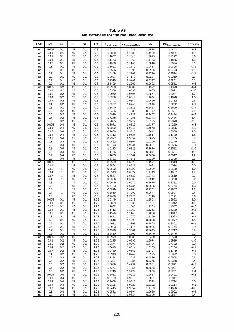
L&P a/T a/c θθ ρρ/T L/T Y plain plate Y Newman & Raju Mk Mk from equation Error (%)

ma 0.005 0.1 45 0.1 0.5 1.0243 1.1031 1.4555 1.4443 -0.8 ma 0.01 0.1 45 0.1 0.5 1.0800 1.1033 1.4130 1.4031 -0.7 ma 0.02 0.1 45 0.1 0.5 1.1047 1.1040 1.3099 1.3172 0.6 ma 0.04 0.1 45 0.1 0.5 1.1443 1.1069 1.1733 1.1885 1.3 ma 0.07 0.1 45 0.1 0.5 1.1558 1.1148 1.0818 1.0824 0.1 ma 0.1 0.1 45 0.1 0.5 1.1692 1.1270 1.0423 1.0308 -1.1 ma 0.2 0.1 45 0.1 0.5 1.2526 1.1990 0.9986 0.9723 -2.6 ma 0.3 0.1 45 0.1 0.5 1.4149 1.3202 0.9720 0.9514 -2.1 ma 0.5 0.1 45 0.1 0.5 1.8967 1.7175 0.9264 0.9310 0.5 ma 0.7 0.1 45 0.1 0.5 2.4518 2.3401 0.8977 0.9251 3.1 ma 0.9 0.1 45 0.1 0.5 2.5409 3.2202 0.9602 0.9551 -0.5 ma 0.005 0.2 45 0.1 0.5 0.9960 1.0589 1.4372 1.4320 -0.4 ma 0.01 0.2 45 0.1 0.5 1.0359 1.0590 1.4065 1.3921 -1.0 ma 0.02 0.2 45 0.1 0.5 1.0059 1.0595 1.2864 1.3087 1.7 ma 0.04 0.2 45 0.1 0.5 1.0359 1.0614 1.1644 1.1826 1.6 ma 0.07 0.2 45 0.1 0.5 1.0741 1.0667 1.0680 1.0762 0.8 ma 0.1 0.2 45 0.1 0.5 1.0927 1.0749 1.0240 1.0232 -0.1 ma 0.2 0.2 45 0.1 0.5 1.1440 1.1221 0.9893 0.9656 -2.4 ma 0.3 0.2 45 0.1 0.5 1.2406 1.1986 0.9772 0.9501 -2.8 ma 0.5 0.2 45 0.1 0.5 1.4976 1.4237 0.9457 0.9424 -0.4 ma 0.7 0.2 45 0.1 0.5 1.7276 1.7055 0.9341 0.9474 1.4 ma 0.9 0.2 45 0.1 0.5 1.7825 1.9772 1.0125 0.9870 -2.5 ma 0.005 0.4 45 0.1 0.5 0.8971 0.9512 1.4377 1.4260 -0.8 ma 0.01 0.4 45 0.1 0.5 0.9292 0.9513 1.4043 1.3855 -1.3 ma 0.02 0.4 45 0.1 0.5 0.9036 0.9515 1.2842 1.3036 1.5 ma 0.04 0.4 45 0.1 0.5 0.9113 0.9525 1.1614 1.1790 1.5 ma 0.07 0.4 45 0.1 0.5 0.9397 0.9552 1.0625 1.0705 0.7 ma 0.1 0.4 45 0.1 0.5 0.9532 0.9594 1.0129 1.0149 0.2 ma 0.2 0.4 45 0.1 0.5 0.9773 0.9834 0.9697 0.9586 -1.1 ma 0.3 0.4 45 0.1 0.5 1.0123 1.0218 0.9676 0.9521 -1.6 ma 0.5 0.4 45 0.1 0.5 1.1156 1.1317 0.9647 0.9627 -0.2 ma 0.7 0.4 45 0.1 0.5 1.1835 1.2587 0.9698 0.9817 1.2 ma 0.9 0.4 45 0.1 0.5 1.2822 1.3575 1.0290 1.0325 0.3 ma 0.005 1 45 0.1 0.5 0.6500 0.6625 1.4571 1.4543 -0.2 ma 0.01 1 45 0.1 0.5 0.6524 0.6626 1.4028 1.4034 0.0 ma 0.02 1 45 0.1 0.5 0.6533 0.6626 1.3050 1.3180 1.0 ma 0.04 1 45 0.1 0.5 0.6543 0.6627 1.1743 1.1937 1.7 ma 0.07 1 45 0.1 0.5 0.6587 0.6632 1.0741 1.0819 0.7 ma 0.1 1 45 0.1 0.5 0.6606 0.6638 1.0212 1.0228 0.2 ma 0.2 1 45 0.1 0.5 0.6649 0.6676 0.9676 0.9722 0.5 ma 0.3 1 45 0.1 0.5 0.6723 0.6736 0.9635 0.9764 1.3 ma 0.5 1 45 0.1 0.5 0.6829 0.6904 0.9742 0.9867 1.3 ma 0.7 1 45 0.1 0.5 0.6819 0.7093 0.9844 0.9887 0.4 ma 0.9 1 45 0.1 0.5 0.7626 0.7223 1.0113 1.0171 0.6 ma 0.005 0.1 45 0.1 1.25 1.0349 1.1031 1.6503 1.6662 1.0 ma 0.01 0.1 45 0.1 1.25 1.0809 1.1033 1.6131 1.6042 -0.5 ma 0.02 0.1 45 0.1 1.25 1.1032 1.1040 1.4959 1.4887 -0.5 ma 0.04 0.1 45 0.1 1.25 1.1413 1.1069 1.3252 1.3220 -0.2 ma 0.07 0.1 45 0.1 1.25 1.1526 1.1148 1.1880 1.1817 -0.5 ma 0.1 0.1 45 0.1 1.25 1.1671 1.1270 1.1120 1.1073 -0.4 ma 0.2 0.1 45 0.1 1.25 1.2516 1.1990 0.9868 0.9977 1.1 ma 0.3 0.1 45 0.1 1.25 1.4021 1.3202 0.9409 0.9401 -0.1 ma 0.5 0.1 45 0.1 1.25 1.8903 1.7175 0.8906 0.8764 -1.6 ma 0.7 0.1 45 0.1 1.25 2.4536 2.3401 0.8649 0.8717 0.8 ma 0.9 0.1 45 0.1 1.25 2.5480 3.2202 0.9440 0.9446 0.1 ma 0.005 0.2 45 0.1 1.25 0.9979 1.0589 1.6480 1.6520 0.2 ma 0.01 0.2 45 0.1 1.25 1.0275 1.0590 1.6074 1.5916 -1.0 ma 0.02 0.2 45 0.1 1.25 1.0144 1.0595 1.4766 1.4792 0.2 ma 0.04 0.2 45 0.1 1.25 1.0448 1.0614 1.3165 1.3154 -0.1 ma 0.07 0.2 45 0.1 1.25 1.0779 1.0667 1.1794 1.1749 -0.4 ma 0.1 0.2 45 0.1 1.25 1.0943 1.0749 1.0995 1.0992 0.0 ma 0.2 0.2 45 0.1 1.25 1.1464 1.1221 0.9880 0.9908 0.3 ma 0.3 0.2 45 0.1 1.25 1.2397 1.1986 0.9355 0.9388 0.4 ma 0.5 0.2 45 0.1 1.25 1.5039 1.4237 0.8901 0.8871 -0.3 ma 0.7 0.2 45 0.1 1.25 1.7251 1.7055 0.8888 0.8927 0.4 ma 0.9 0.2 45 0.1 1.25 1.7713 1.9772 1.0005 0.9761 -2.4 ma 0.005 0.4 45 0.1 1.25 0.8982 0.9512 1.6487 1.6451 -0.2 ma 0.01 0.4 45 0.1 1.25 0.9109 0.9513 1.6031 1.5841 -1.2 ma 0.02 0.4 45 0.1 1.25 0.9066 0.9515 1.4728 1.4734 0.0 ma 0.04 0.4 45 0.1 1.25 0.9155 0.9525 1.3132 1.3114 -0.1 ma 0.07 0.4 45 0.1 1.25 0.9415 0.9552 1.1783 1.1686 -0.8 ma 0.1 0.4 45 0.1 1.25 0.9531 0.9594 1.0969 1.0902 -0.6 ma 0.2 0.4 45 0.1 1.25 0.9747 0.9834 0.9800 0.9837 0.4

Table A5Mk database for the radiused weld toe

228

L&P a/T a/c θθ ρρ/T L/T Y plain plate Y Newman & Raju Mk Mk from equation Error (%)

ma 0.3 0.4 45 0.1 1.25 1.0094 1.0218 0.9393 0.9407 0.2 ma 0.5 0.4 45 0.1 1.25 1.1055 1.1317 0.9065 0.9062 0.0 ma 0.7 0.4 45 0.1 1.25 1.1828 1.2587 0.9199 0.9250 0.6 ma 0.9 0.4 45 0.1 1.25 1.2553 1.3575 1.0249 1.0211 -0.4 ma 0.005 1 45 0.1 1.25 0.6497 0.6625 1.6643 1.6777 0.8 ma 0.01 1 45 0.1 1.25 0.6520 0.6626 1.6044 1.6046 0.0 ma 0.02 1 45 0.1 1.25 0.6525 0.6626 1.4914 1.4897 -0.1 ma 0.04 1 45 0.1 1.25 0.6545 0.6627 1.3266 1.3277 0.1 ma 0.07 1 45 0.1 1.25 0.6591 0.6632 1.1926 1.1812 -1.0 ma 0.1 1 45 0.1 1.25 0.6609 0.6638 1.1097 1.0988 -1.0 ma 0.2 1 45 0.1 1.25 0.6649 0.6676 0.9904 0.9976 0.7 ma 0.3 1 45 0.1 1.25 0.6719 0.6736 0.9528 0.9648 1.3 ma 0.5 1 45 0.1 1.25 0.6827 0.6904 0.9382 0.9288 -1.0 ma 0.7 1 45 0.1 1.25 0.6725 0.7093 0.9578 0.9317 -2.7 ma 0.9 1 45 0.1 1.25 0.7811 0.7223 1.0115 1.0058 -0.6 ma 0.005 0.1 45 0.1 2 1.0276 1.1031 1.6768 1.6789 0.1 ma 0.01 0.1 45 0.1 2 1.0208 1.1033 1.6115 1.6235 0.7 ma 0.02 0.1 45 0.1 2 1.0526 1.1040 1.5113 1.5122 0.1 ma 0.04 0.1 45 0.1 2 1.1455 1.1069 1.3416 1.3451 0.3 ma 0.07 0.1 45 0.1 2 1.1567 1.1148 1.1976 1.2001 0.2 ma 0.1 0.1 45 0.1 2 1.1703 1.1270 1.1143 1.1203 0.5 ma 0.2 0.1 45 0.1 2 1.2563 1.1990 0.9843 0.9923 0.8 ma 0.3 0.1 45 0.1 2 1.4074 1.3202 0.9174 0.9187 0.2 ma 0.5 0.1 45 0.1 2 1.8902 1.7175 0.8470 0.8374 -1.1 ma 0.7 0.1 45 0.1 2 2.4534 2.3401 0.8142 0.8377 2.9 ma 0.9 0.1 45 0.1 2 2.5451 3.2202 0.9196 0.9328 1.4 ma 0.005 0.2 45 0.1 2 0.9979 1.0589 1.6634 1.6647 0.1 ma 0.01 0.2 45 0.1 2 1.0269 1.0590 1.6274 1.6107 -1.0 ma 0.02 0.2 45 0.1 2 1.0150 1.0595 1.4988 1.5025 0.2 ma 0.04 0.2 45 0.1 2 1.0474 1.0614 1.3334 1.3384 0.4 ma 0.07 0.2 45 0.1 2 1.0797 1.0667 1.1905 1.1932 0.2 ma 0.1 0.2 45 0.1 2 1.0953 1.0749 1.1047 1.1120 0.7 ma 0.2 0.2 45 0.1 2 1.1480 1.1221 0.9734 0.9853 1.2 ma 0.3 0.2 45 0.1 2 1.2401 1.1986 0.9097 0.9175 0.9 ma 0.5 0.2 45 0.1 2 1.5009 1.4237 0.8518 0.8477 -0.5 ma 0.7 0.2 45 0.1 2 1.7262 1.7055 0.8426 0.8580 1.8 ma 0.9 0.2 45 0.1 2 1.7993 1.9772 0.9834 0.9639 -2.0 ma 0.005 0.4 45 0.1 2 0.8983 0.9512 1.6668 1.6577 -0.6 ma 0.01 0.4 45 0.1 2 0.9107 0.9513 1.6222 1.6031 -1.2 ma 0.02 0.4 45 0.1 2 0.9067 0.9515 1.4947 1.4967 0.1 ma 0.04 0.4 45 0.1 2 0.9167 0.9525 1.3299 1.3343 0.3 ma 0.07 0.4 45 0.1 2 0.9423 0.9552 1.1901 1.1869 -0.3 ma 0.1 0.4 45 0.1 2 0.9533 0.9594 1.1036 1.1029 -0.1 ma 0.2 0.4 45 0.1 2 0.9748 0.9834 0.9715 0.9783 0.7 ma 0.3 0.4 45 0.1 2 1.0100 1.0218 0.9169 0.9194 0.3 ma 0.5 0.4 45 0.1 2 1.1067 1.1317 0.8772 0.8660 -1.3 ma 0.7 0.4 45 0.1 2 1.1819 1.2587 0.8760 0.8890 1.5 ma 0.9 0.4 45 0.1 2 1.2926 1.3575 1.0109 1.0083 -0.3 ma 0.005 1 45 0.1 2 0.6431 0.6625 1.6802 1.6905 0.6 ma 0.01 1 45 0.1 2 0.6505 0.6626 1.6208 1.6238 0.2 ma 0.02 1 45 0.1 2 0.6513 0.6626 1.5084 1.5132 0.3 ma 0.04 1 45 0.1 2 0.6541 0.6627 1.3435 1.3510 0.6 ma 0.07 1 45 0.1 2 0.6586 0.6632 1.2047 1.1996 -0.4 ma 0.1 1 45 0.1 2 0.6606 0.6638 1.1169 1.1116 -0.5 ma 0.2 1 45 0.1 2 0.6654 0.6676 0.9848 0.9921 0.7 ma 0.3 1 45 0.1 2 0.6717 0.6736 0.9369 0.9429 0.6 ma 0.5 1 45 0.1 2 0.6829 0.6904 0.9085 0.8875 -2.3 ma 0.7 1 45 0.1 2 0.6726 0.7093 0.9203 0.8954 -2.7 ma 0.9 1 45 0.1 2 0.7677 0.7223 0.9704 0.9933 2.4 ma 0.005 0.1 45 0.1 2.75 1.0246 1.1031 1.6796 1.6925 0.8 ma 0.01 0.1 45 0.1 2.75 1.0796 1.1033 1.6530 1.6316 -1.3 ma 0.02 0.1 45 0.1 2.75 1.1052 1.1040 1.5357 1.5174 -1.2 ma 0.04 0.1 45 0.1 2.75 1.1272 1.1069 1.3588 1.3494 -0.7 ma 0.07 0.1 45 0.1 2.75 1.1514 1.1148 1.2078 1.2040 -0.3 ma 0.1 0.1 45 0.1 2.75 1.1569 1.1270 1.1217 1.1234 0.2 ma 0.2 0.1 45 0.1 2.75 1.2459 1.1990 0.9735 0.9904 1.7 ma 0.3 0.1 45 0.1 2.75 1.3981 1.3202 0.9095 0.9097 0.0 ma 0.5 0.1 45 0.1 2.75 1.8938 1.7175 0.8205 0.8127 -1.0 ma 0.7 0.1 45 0.1 2.75 2.4545 2.3401 0.7802 0.8037 3.0 ma 0.9 0.1 45 0.1 2.75 2.5493 3.2202 0.9011 0.9067 0.6 ma 0.005 0.2 45 0.1 2.75 0.9878 1.0589 1.6341 1.6781 2.7 ma 0.01 0.2 45 0.1 2.75 1.0054 1.0590 1.6183 1.6187 0.0 ma 0.02 0.2 45 0.1 2.75 1.0057 1.0595 1.5049 1.5077 0.2 ma 0.04 0.2 45 0.1 2.75 1.0334 1.0614 1.3436 1.3427 -0.1 ma 0.07 0.2 45 0.1 2.75 1.0442 1.0667 1.1967 1.1970 0.0 ma 0.1 0.2 45 0.1 2.75 1.0722 1.0749 1.1103 1.1151 0.4 ma 0.2 0.2 45 0.1 2.75 1.1351 1.1221 0.9694 0.9835 1.5

229

L&P a/T a/c θθ ρρ/T L/T Y plain plate Y Newman & Raju Mk Mk from equation Error (%)

ma 0.3 0.2 45 0.1 2.75 1.2335 1.1986 0.9008 0.9084 0.8 ma 0.5 0.2 45 0.1 2.75 1.4951 1.4237 0.8206 0.8226 0.2 ma 0.7 0.2 45 0.1 2.75 1.7250 1.7055 0.8177 0.8231 0.7 ma 0.9 0.2 45 0.1 2.75 1.7977 1.9772 0.9699 0.9370 -3.4 ma 0.005 0.4 45 0.1 2.75 0.8928 0.9512 1.6422 1.6711 1.8 ma 0.01 0.4 45 0.1 2.75 0.9040 0.9513 1.6220 1.6112 -0.7 ma 0.02 0.4 45 0.1 2.75 0.9039 0.9515 1.5021 1.5019 0.0 ma 0.04 0.4 45 0.1 2.75 0.9088 0.9525 1.3402 1.3386 -0.1 ma 0.07 0.4 45 0.1 2.75 0.9255 0.9552 1.1957 1.1907 -0.4 ma 0.1 0.4 45 0.1 2.75 0.9422 0.9594 1.1088 1.1060 -0.3 ma 0.2 0.4 45 0.1 2.75 0.9699 0.9834 0.9686 0.9765 0.8 ma 0.3 0.4 45 0.1 2.75 1.0123 1.0218 0.9070 0.9103 0.4 ma 0.5 0.4 45 0.1 2.75 1.1136 1.1317 0.8474 0.8404 -0.8 ma 0.7 0.4 45 0.1 2.75 1.1823 1.2587 0.8509 0.8528 0.2 ma 0.9 0.4 45 0.1 2.75 1.2928 1.3575 0.9840 0.9802 -0.4 ma 0.005 1 45 0.1 2.75 0.6436 0.6625 1.7416 1.7042 -2.2 ma 0.01 1 45 0.1 2.75 0.6505 0.6626 1.6361 1.6320 -0.3 ma 0.02 1 45 0.1 2.75 0.6514 0.6626 1.5256 1.5184 -0.5 ma 0.04 1 45 0.1 2.75 0.6506 0.6627 1.3535 1.3553 0.1 ma 0.07 1 45 0.1 2.75 0.6565 0.6632 1.2127 1.2034 -0.8 ma 0.1 1 45 0.1 2.75 0.6591 0.6638 1.1224 1.1147 -0.7 ma 0.2 1 45 0.1 2.75 0.6641 0.6676 0.9824 0.9903 0.8 ma 0.3 1 45 0.1 2.75 0.6715 0.6736 0.9281 0.9336 0.6 ma 0.5 1 45 0.1 2.75 0.6831 0.6904 0.8887 0.8613 -3.1 ma 0.7 1 45 0.1 2.75 0.6726 0.7093 0.8906 0.8590 -3.6 ma 0.9 1 45 0.1 2.75 0.7640 0.7223 0.9320 0.9655 3.6 ba 0.005 0.1 45 0.1 0.5 1.0542 1.0963 1.4051 1.4017 -0.2 ba 0.01 0.1 45 0.1 0.5 1.1051 1.0898 1.3682 1.3569 -0.8 ba 0.02 0.1 45 0.1 0.5 1.1162 1.0770 1.2742 1.2738 0.0 ba 0.04 0.1 45 0.1 0.5 1.1285 1.0530 1.1412 1.1507 0.8 ba 0.07 0.1 45 0.1 0.5 1.0970 1.0207 1.0499 1.0473 -0.2 ba 0.1 0.1 45 0.1 0.5 1.0667 0.9924 1.0069 1.0004 -0.6 ba 0.2 0.1 45 0.1 0.5 1.0009 0.9217 1.0032 0.9775 -2.6 ba 0.3 0.1 45 0.1 0.5 0.9819 0.8772 0.9797 0.9869 0.7 ba 0.5 0.1 45 0.1 0.5 0.9789 0.8219 0.9342 0.9847 5.4 ba 0.7 0.1 45 0.1 0.5 0.8857 0.7556 0.8856 1.0000 12.9 ba 0.9 0.1 45 0.1 0.5 0.2685 0.6360 0.9425 1.0000 6.1 ba 0.005 0.2 45 0.1 0.5 1.0246 1.0523 1.3872 1.3915 0.3 ba 0.01 0.2 45 0.1 0.5 1.0590 1.0459 1.3620 1.3443 -1.3 ba 0.02 0.2 45 0.1 0.5 1.0149 1.0333 1.2501 1.2598 0.8 ba 0.04 0.2 45 0.1 0.5 1.0204 1.0091 1.1310 1.1354 0.4 ba 0.07 0.2 45 0.1 0.5 1.0180 0.9753 1.0355 1.0286 -0.7 ba 0.1 0.2 45 0.1 0.5 0.9947 0.9441 0.9884 0.9765 -1.2 ba 0.2 0.2 45 0.1 0.5 0.9024 0.8554 0.9414 0.9367 -0.5 ba 0.3 0.2 45 0.1 0.5 0.8411 0.7813 0.9542 0.9375 -1.8 ba 0.5 0.2 45 0.1 0.5 0.7208 0.6371 0.9344 0.9373 0.3 ba 0.7 0.2 45 0.1 0.5 0.5064 0.4527 0.9023 1.0000 10.8 ba 0.9 0.2 45 0.1 0.5 0.0223 0.2088 0.6524 1.0000 53.3 ba 0.005 0.4 45 0.1 0.5 0.9222 0.9452 1.3885 1.3889 0.0 ba 0.01 0.4 45 0.1 0.5 0.9505 0.9392 1.3588 1.3421 -1.2 ba 0.02 0.4 45 0.1 0.5 0.9103 0.9274 1.2473 1.2601 1.0 ba 0.04 0.4 45 0.1 0.5 0.8958 0.9044 1.1272 1.1400 1.1 ba 0.07 0.4 45 0.1 0.5 0.8874 0.8711 1.0291 1.0335 0.4 ba 0.1 0.4 45 0.1 0.5 0.8633 0.8391 0.9758 0.9769 0.1 ba 0.2 0.4 45 0.1 0.5 0.7607 0.7395 0.9188 0.9148 -0.4 ba 0.3 0.4 45 0.1 0.5 0.6636 0.6461 0.9075 0.9003 -0.8 ba 0.5 0.4 45 0.1 0.5 0.4768 0.4540 0.9120 0.8923 -2.2 ba 0.7 0.4 45 0.1 0.5 0.2348 0.2283 0.9323 1.0000 7.3 ba 0.9 0.4 45 0.1 0.5 -0.1740 -0.0369 0.7556 1.0000 32.3 ba 0.005 1 45 0.1 0.5 0.6665 0.6581 1.3984 1.4088 0.7 ba 0.01 1 45 0.1 0.5 0.6641 0.6537 1.3586 1.3572 -0.1 ba 0.02 1 45 0.1 0.5 0.6549 0.6448 1.2708 1.2713 0.0 ba 0.04 1 45 0.1 0.5 0.6378 0.6272 1.1406 1.1504 0.9 ba 0.07 1 45 0.1 0.5 0.6133 0.6009 1.0402 1.0469 0.6 ba 0.1 1 45 0.1 0.5 0.5863 0.5747 0.9822 0.9919 1.0 ba 0.2 1 45 0.1 0.5 0.4936 0.4879 0.9108 0.9222 1.3 ba 0.3 1 45 0.1 0.5 0.4037 0.4010 0.8911 0.8940 0.3 ba 0.5 1 45 0.1 0.5 0.2152 0.2227 0.8902 0.8607 -3.3 ba 0.7 1 45 0.1 0.5 0.0172 0.0335 0.5030 1.0000 98.8 ba 0.9 1 45 0.1 0.5 -0.2622 -0.1663 0.8602 1.0000 16.2 ba 0.005 0.1 45 0.1 1.25 1.0651 1.0963 1.5806 1.5937 0.8 ba 0.01 0.1 45 0.1 1.25 1.1059 1.0898 1.5510 1.5427 -0.5 ba 0.02 0.1 45 0.1 1.25 1.1146 1.0770 1.4465 1.4420 -0.3 ba 0.04 0.1 45 0.1 1.25 1.1256 1.0530 1.2814 1.2859 0.3 ba 0.07 0.1 45 0.1 1.25 1.0940 1.0207 1.1428 1.1448 0.2 ba 0.1 0.1 45 0.1 1.25 1.0648 0.9924 1.0583 1.0690 1.0 ba 0.2 0.1 45 0.1 1.25 1.0001 0.9217 0.9744 0.9700 -0.4

230

L&P a/T a/c θθ ρρ/T L/T Y plain plate Y Newman & Raju Mk Mk from equation Error (%)

ba 0.3 0.1 45 0.1 1.25 0.9740 0.8772 0.9301 0.9161 -1.5 ba 0.5 0.1 45 0.1 1.25 0.9755 0.8219 0.8679 0.8310 -4.3 ba 0.7 0.1 45 0.1 1.25 0.8863 0.7556 0.8136 1.0000 22.9 ba 0.9 0.1 45 0.1 1.25 0.2666 0.6360 0.8361 1.0000 19.6 ba 0.005 0.2 45 0.1 1.25 1.0266 1.0523 1.5774 1.5821 0.3 ba 0.01 0.2 45 0.1 1.25 1.0508 1.0459 1.5443 1.5285 -1.0 ba 0.02 0.2 45 0.1 1.25 1.0238 1.0333 1.4253 1.4261 0.1 ba 0.04 0.2 45 0.1 1.25 1.0294 1.0091 1.2705 1.2688 -0.1 ba 0.07 0.2 45 0.1 1.25 1.0217 0.9753 1.1336 1.1244 -0.8 ba 0.1 0.2 45 0.1 1.25 0.9961 0.9441 1.0460 1.0434 -0.2 ba 0.2 0.2 45 0.1 1.25 0.9043 0.8554 0.9021 0.9294 3.0 ba 0.3 0.2 45 0.1 1.25 0.8404 0.7813 0.8659 0.8702 0.5 ba 0.5 0.2 45 0.1 1.25 0.7238 0.6371 0.8146 0.7910 -2.9 ba 0.7 0.2 45 0.1 1.25 0.5050 0.4527 0.7791 1.0000 28.3 ba 0.9 0.2 45 0.1 1.25 0.0229 0.2088 0.8774 1.0000 14.0 ba 0.005 0.4 45 0.1 1.25 0.9234 0.9452 1.5786 1.5791 0.0 ba 0.01 0.4 45 0.1 1.25 0.9309 0.9392 1.5404 1.5259 -0.9 ba 0.02 0.4 45 0.1 1.25 0.9137 0.9274 1.4213 1.4265 0.4 ba 0.04 0.4 45 0.1 1.25 0.9002 0.9044 1.2662 1.2739 0.6 ba 0.07 0.4 45 0.1 1.25 0.8893 0.8711 1.1321 1.1298 -0.2 ba 0.1 0.4 45 0.1 1.25 0.8633 0.8391 1.0431 1.0439 0.1 ba 0.2 0.4 45 0.1 1.25 0.7584 0.7395 0.8915 0.9077 1.8 ba 0.3 0.4 45 0.1 1.25 0.6616 0.6461 0.8191 0.8358 2.0 ba 0.5 0.4 45 0.1 1.25 0.4721 0.4540 0.7522 0.7531 0.1 ba 0.7 0.4 45 0.1 1.25 0.2352 0.2283 0.7097 1.0000 40.9 ba 0.9 0.4 45 0.1 1.25 -0.1774 -0.0369 0.8115 1.0000 23.2 ba 0.005 1 45 0.1 1.25 0.6661 0.6581 1.5879 1.6017 0.9 ba 0.01 1 45 0.1 1.25 0.6635 0.6537 1.5436 1.5431 0.0 ba 0.02 1 45 0.1 1.25 0.6539 0.6448 1.4445 1.4391 -0.4 ba 0.04 1 45 0.1 1.25 0.6382 0.6272 1.2819 1.2856 0.3 ba 0.07 1 45 0.1 1.25 0.6137 0.6009 1.1476 1.1444 -0.3 ba 0.1 1 45 0.1 1.25 0.5866 0.5747 1.0553 1.0600 0.4 ba 0.2 1 45 0.1 1.25 0.4938 0.4879 0.8933 0.9150 2.4 ba 0.3 1 45 0.1 1.25 0.4029 0.4010 0.8141 0.8299 1.9 ba 0.5 1 45 0.1 1.25 0.2151 0.2227 0.7038 0.7264 3.2 ba 0.7 1 45 0.1 1.25 0.0287 0.0335 -1.0015 1.0000 -199.9 ba 0.9 1 45 0.1 1.25 -0.2416 -0.1663 0.8573 1.0000 16.7 ba 0.005 0.1 45 0.1 2 1.0574 1.0963 1.6172 1.6152 -0.1 ba 0.01 0.1 45 0.1 2 1.0439 1.0898 1.5626 1.5765 0.9 ba 0.02 0.1 45 0.1 2 1.0631 1.0770 1.4800 1.4822 0.2 ba 0.04 0.1 45 0.1 2 1.1296 1.0530 1.3163 1.3224 0.5 ba 0.07 0.1 45 0.1 2 1.0977 1.0207 1.1701 1.1695 -0.1 ba 0.1 0.1 45 0.1 2 1.0677 0.9924 1.0770 1.0819 0.5 ba 0.2 0.1 45 0.1 2 1.0036 0.9217 0.9535 0.9498 -0.4 ba 0.3 0.1 45 0.1 2 0.9774 0.8772 0.8895 0.8740 -1.7 ba 0.5 0.1 45 0.1 2 0.9755 0.8219 0.7972 0.7813 -2.0 ba 0.7 0.1 45 0.1 2 0.8861 0.7556 0.7234 1.0000 38.2 ba 0.9 0.1 45 0.1 2 0.2674 0.6360 0.7081 1.0000 41.2 ba 0.005 0.2 45 0.1 2 1.0267 1.0523 1.5997 1.6035 0.2 ba 0.01 0.2 45 0.1 2 1.0502 1.0459 1.5784 1.5620 -1.0 ba 0.02 0.2 45 0.1 2 1.0245 1.0333 1.4654 1.4658 0.0 ba 0.04 0.2 45 0.1 2 1.0321 1.0091 1.3051 1.3048 0.0 ba 0.07 0.2 45 0.1 2 1.0234 0.9753 1.1622 1.1486 -1.2 ba 0.1 0.2 45 0.1 2 0.9971 0.9441 1.0675 1.0560 -1.1 ba 0.2 0.2 45 0.1 2 0.9056 0.8554 0.8992 0.9101 1.2 ba 0.3 0.2 45 0.1 2 0.8407 0.7813 0.8225 0.8303 0.9 ba 0.5 0.2 45 0.1 2 0.7220 0.6371 0.7347 0.7437 1.2 ba 0.7 0.2 45 0.1 2 0.5055 0.4527 0.6725 1.0000 48.7 ba 0.9 0.2 45 0.1 2 0.0161 0.2088 -1.9674 1.0000 -150.8 ba 0.005 0.4 45 0.1 2 0.9235 0.9452 1.6047 1.6005 -0.3 ba 0.01 0.4 45 0.1 2 0.9307 0.9392 1.5738 1.5594 -0.9 ba 0.02 0.4 45 0.1 2 0.9138 0.9274 1.4612 1.4662 0.3 ba 0.04 0.4 45 0.1 2 0.9014 0.9044 1.3008 1.3101 0.7 ba 0.07 0.4 45 0.1 2 0.8901 0.8711 1.1619 1.1542 -0.7 ba 0.1 0.4 45 0.1 2 0.8636 0.8391 1.0668 1.0566 -1.0 ba 0.2 0.4 45 0.1 2 0.7585 0.7395 0.8954 0.8888 -0.7 ba 0.3 0.4 45 0.1 2 0.6620 0.6461 0.8031 0.7974 -0.7 ba 0.5 0.4 45 0.1 2 0.4728 0.4540 0.6913 0.7080 2.4 ba 0.7 0.4 45 0.1 2 0.2349 0.2283 0.5974 1.0000 67.4 ba 0.9 0.4 45 0.1 2 -0.1734 -0.0369 0.8683 1.0000 15.2 ba 0.005 1 45 0.1 2 0.6591 0.6581 1.6068 1.6233 1.0 ba 0.01 1 45 0.1 2 0.6618 0.6537 1.5714 1.5770 0.4 ba 0.02 1 45 0.1 2 0.6527 0.6448 1.4814 1.4792 -0.1 ba 0.04 1 45 0.1 2 0.6376 0.6272 1.3193 1.3221 0.2 ba 0.07 1 45 0.1 2 0.6131 0.6009 1.1804 1.1691 -1.0 ba 0.1 1 45 0.1 2 0.5863 0.5747 1.0820 1.0728 -0.9 ba 0.2 1 45 0.1 2 0.4943 0.4879 0.9018 0.8960 -0.6

231

L&P a/T a/c θθ ρρ/T L/T Y plain plate Y Newman & Raju Mk Mk from equation Error (%)

ba 0.3 1 45 0.1 2 0.4027 0.4010 0.8056 0.7917 -1.7 ba 0.5 1 45 0.1 2 0.2152 0.2227 0.6624 0.6829 3.1 ba 0.7 1 45 0.1 2 0.0278 0.0335 -0.7596 1.0000 -231.6 ba 0.9 1 45 0.1 2 -0.2243 -0.1663 0.8692 1.0000 15.0 ba 0.005 0.1 45 0.1 2.75 1.0543 1.0963 1.6084 1.6096 0.1 ba 0.01 0.1 45 0.1 2.75 1.1043 1.0898 1.5996 1.5770 -1.4 ba 0.02 0.1 45 0.1 2.75 1.1164 1.0770 1.5000 1.4896 -0.7 ba 0.04 0.1 45 0.1 2.75 1.1110 1.0530 1.3319 1.3352 0.3 ba 0.07 0.1 45 0.1 2.75 1.0921 1.0207 1.1810 1.1840 0.3 ba 0.1 0.1 45 0.1 2.75 1.0553 0.9924 1.0866 1.0955 0.8 ba 0.2 0.1 45 0.1 2.75 0.9960 0.9217 0.9324 0.9541 2.3 ba 0.3 0.1 45 0.1 2.75 0.9719 0.8772 0.8530 0.8647 1.4 ba 0.5 0.1 45 0.1 2.75 0.9773 0.8219 0.7505 0.7439 -0.9 ba 0.7 0.1 45 0.1 2.75 0.8868 0.7556 0.6630 1.0000 50.8 ba 0.9 0.1 45 0.1 2.75 0.2666 0.6360 0.6197 1.0000 61.4 ba 0.005 0.2 45 0.1 2.75 1.0154 1.0523 1.5590 1.5979 2.5 ba 0.01 0.2 45 0.1 2.75 1.0272 1.0459 1.5592 1.5625 0.2 ba 0.02 0.2 45 0.1 2.75 1.0144 1.0333 1.4657 1.4731 0.5 ba 0.04 0.2 45 0.1 2.75 1.0170 1.0091 1.3139 1.3175 0.3 ba 0.07 0.2 45 0.1 2.75 0.9884 0.9753 1.1685 1.1628 -0.5 ba 0.1 0.2 45 0.1 2.75 0.9753 0.9441 1.0753 1.0693 -0.6 ba 0.2 0.2 45 0.1 2.75 0.8955 0.8554 0.9005 0.9143 1.5 ba 0.3 0.2 45 0.1 2.75 0.8364 0.7813 0.8098 0.8214 1.4 ba 0.5 0.2 45 0.1 2.75 0.7193 0.6371 0.6973 0.7081 1.5 ba 0.7 0.2 45 0.1 2.75 0.5053 0.4527 0.6056 1.0000 65.1 ba 0.9 0.2 45 0.1 2.75 0.0185 0.2088 -2.3893 1.0000 -141.9 ba 0.005 0.4 45 0.1 2.75 0.9172 0.9452 1.5783 1.5949 1.1 ba 0.01 0.4 45 0.1 2.75 0.9230 0.9392 1.5698 1.5598 -0.6 ba 0.02 0.4 45 0.1 2.75 0.9104 0.9274 1.4653 1.4735 0.6 ba 0.04 0.4 45 0.1 2.75 0.8924 0.9044 1.3106 1.3228 0.9 ba 0.07 0.4 45 0.1 2.75 0.8728 0.8711 1.1686 1.1685 0.0 ba 0.1 0.4 45 0.1 2.75 0.8525 0.8391 1.0740 1.0698 -0.4 ba 0.2 0.4 45 0.1 2.75 0.7546 0.7395 0.8981 0.8929 -0.6 ba 0.3 0.4 45 0.1 2.75 0.6626 0.6461 0.8019 0.7888 -1.6 ba 0.5 0.4 45 0.1 2.75 0.4757 0.4540 0.6692 0.6741 0.7 ba 0.7 0.4 45 0.1 2.75 0.2340 0.2283 0.5481 1.0000 82.5 ba 0.9 0.4 45 0.1 2.75 -0.1730 -0.0369 0.8929 1.0000 12.0 ba 0.005 1 45 0.1 2.75 0.6596 0.6581 1.6496 1.6177 -1.9 ba 0.01 1 45 0.1 2.75 0.6618 0.6537 1.5804 1.5775 -0.2 ba 0.02 1 45 0.1 2.75 0.6528 0.6448 1.4939 1.4865 -0.5 ba 0.04 1 45 0.1 2.75 0.6331 0.6272 1.3291 1.3349 0.4 ba 0.07 1 45 0.1 2.75 0.6102 0.6009 1.1911 1.1835 -0.6 ba 0.1 1 45 0.1 2.75 0.5840 0.5747 1.0917 1.0863 -0.5 ba 0.2 1 45 0.1 2.75 0.4925 0.4879 0.9077 0.9001 -0.8 ba 0.3 1 45 0.1 2.75 0.4022 0.4010 0.8073 0.7833 -3.0 ba 0.5 1 45 0.1 2.75 0.2154 0.2227 0.6544 0.6502 -0.6 ba 0.7 1 45 0.1 2.75 0.0276 0.0335 -0.6125 1.0000 -263.3 ba 0.9 1 45 0.1 2.75 -0.2206 -0.1663 0.8832 1.0000 13.2 mc 0.005 0.1 45 0.1 0.5 0.4097 0.3837 2.4203 2.4901 2.9 mc 0.01 0.1 45 0.1 0.5 0.3787 0.3838 2.1566 2.1697 0.6 mc 0.02 0.1 45 0.1 0.5 0.3769 0.3841 1.9158 1.9231 0.4 mc 0.04 0.1 45 0.1 0.5 0.3792 0.3852 1.8091 1.7760 -1.8 mc 0.07 0.1 45 0.1 0.5 0.3900 0.3884 1.7138 1.6901 -1.4 mc 0.1 0.1 45 0.1 0.5 0.3987 0.3933 1.6552 1.6379 -1.0 mc 0.2 0.1 45 0.1 0.5 0.4223 0.4224 1.5404 1.5377 -0.2 mc 0.3 0.1 45 0.1 0.5 0.4515 0.4724 1.4664 1.4776 0.8 mc 0.5 0.1 45 0.1 0.5 0.5599 0.6449 1.3639 1.3905 2.0 mc 0.7 0.1 45 0.1 0.5 0.8518 0.9409 1.2504 1.3126 5.0 mc 0.9 0.1 45 0.1 0.5 1.2246 1.4088 1.1800 1.2311 4.3 mc 0.005 0.2 45 0.1 0.5 0.5230 0.5209 1.7898 1.8822 5.2 mc 0.01 0.2 45 0.1 0.5 0.4809 0.5210 1.8052 1.7982 -0.4 mc 0.02 0.2 45 0.1 0.5 0.4913 0.5213 1.7099 1.7164 0.4 mc 0.04 0.2 45 0.1 0.5 0.4733 0.5224 1.6431 1.6361 -0.4 mc 0.07 0.2 45 0.1 0.5 0.4986 0.5256 1.5812 1.5691 -0.8 mc 0.1 0.2 45 0.1 0.5 0.5119 0.5304 1.5337 1.5233 -0.7 mc 0.2 0.2 45 0.1 0.5 0.5402 0.5590 1.4425 1.4249 -1.2 mc 0.3 0.2 45 0.1 0.5 0.5791 0.6065 1.3767 1.3621 -1.1 mc 0.5 0.2 45 0.1 0.5 0.7160 0.7561 1.2736 1.2708 -0.2 mc 0.7 0.2 45 0.1 0.5 0.9970 0.9698 1.1753 1.1904 1.3 mc 0.9 0.2 45 0.1 0.5 1.3055 1.2233 1.1166 1.1080 -0.8 mc 0.005 0.4 45 0.1 0.5 0.6372 0.6618 1.5395 1.6894 9.7 mc 0.01 0.4 45 0.1 0.5 0.6127 0.6618 1.6735 1.6521 -1.3 mc 0.02 0.4 45 0.1 0.5 0.6127 0.6621 1.5910 1.6017 0.7 mc 0.04 0.4 45 0.1 0.5 0.5984 0.6630 1.5234 1.5364 0.9 mc 0.07 0.4 45 0.1 0.5 0.6267 0.6656 1.4518 1.4719 1.4 mc 0.1 0.4 45 0.1 0.5 0.6400 0.6696 1.3988 1.4257 1.9 mc 0.2 0.4 45 0.1 0.5 0.6638 0.6928 1.3161 1.3297 1.0

232

L&P a/T a/c θθ ρρ/T L/T Y plain plate Y Newman & Raju Mk Mk from equation Error (%)

mc 0.3 0.4 45 0.1 0.5 0.6954 0.7312 1.2904 1.2762 -1.1 mc 0.5 0.4 45 0.1 0.5 0.8113 0.8499 1.2295 1.2179 -0.9 mc 0.7 0.4 45 0.1 0.5 0.9763 1.0122 1.1895 1.1775 -1.0 mc 0.9 0.4 45 0.1 0.5 1.1618 1.1878 1.1343 1.1318 -0.2 mc 0.005 1 45 0.1 0.5 0.7041 0.7288 1.5795 1.6361 3.6 mc 0.01 1 45 0.1 0.5 0.7023 0.7288 1.6041 1.6077 0.2 mc 0.02 1 45 0.1 0.5 0.7038 0.7289 1.5591 1.5584 0.0 mc 0.04 1 45 0.1 0.5 0.7040 0.7294 1.4679 1.4819 1.0 mc 0.07 1 45 0.1 0.5 0.7118 0.7306 1.3814 1.3977 1.2 mc 0.1 1 45 0.1 0.5 0.7149 0.7325 1.3173 1.3353 1.4 mc 0.2 1 45 0.1 0.5 0.7220 0.7437 1.2089 1.2137 0.4 mc 0.3 1 45 0.1 0.5 0.7358 0.7621 1.1704 1.1635 -0.6 mc 0.5 1 45 0.1 0.5 0.7761 0.8199 1.1610 1.1445 -1.4 mc 0.7 1 45 0.1 0.5 0.8281 0.9018 1.1753 1.1467 -2.4 mc 0.9 1 45 0.1 0.5 0.8974 0.9993 1.1657 1.1364 -2.5 mc 0.005 0.1 45 0.1 1.25 0.4189 0.3837 2.8626 2.8721 0.3 mc 0.01 0.1 45 0.1 1.25 0.3876 0.3838 2.5223 2.5198 -0.1 mc 0.02 0.1 45 0.1 1.25 0.3843 0.3841 2.2295 2.2427 0.6 mc 0.04 0.1 45 0.1 1.25 0.3780 0.3852 2.0934 2.0688 -1.2 mc 0.07 0.1 45 0.1 1.25 0.3886 0.3884 1.9704 1.9571 -0.7 mc 0.1 0.1 45 0.1 1.25 0.3978 0.3933 1.8978 1.8855 -0.6 mc 0.2 0.1 45 0.1 1.25 0.4196 0.4224 1.7350 1.7412 0.4 mc 0.3 0.1 45 0.1 1.25 0.4486 0.4724 1.6477 1.6470 0.0 mc 0.5 0.1 45 0.1 1.25 0.5588 0.6449 1.5343 1.5049 -1.9 mc 0.7 0.1 45 0.1 1.25 0.8552 0.9409 1.3922 1.3898 -0.2 mc 0.9 0.1 45 0.1 1.25 1.2436 1.4088 1.3010 1.2886 -1.0 mc 0.005 0.2 45 0.1 1.25 0.5194 0.5209 2.1223 2.1489 1.2 mc 0.01 0.2 45 0.1 1.25 0.4846 0.5210 2.0686 2.0676 0.0 mc 0.02 0.2 45 0.1 1.25 0.4883 0.5213 1.9542 1.9821 1.4 mc 0.04 0.2 45 0.1 1.25 0.4751 0.5224 1.8850 1.8871 0.1 mc 0.07 0.2 45 0.1 1.25 0.4996 0.5256 1.8042 1.7987 -0.3 mc 0.1 0.2 45 0.1 1.25 0.5123 0.5304 1.7371 1.7354 -0.1 mc 0.2 0.2 45 0.1 1.25 0.5403 0.5590 1.6097 1.5959 -0.9 mc 0.3 0.2 45 0.1 1.25 0.5792 0.6065 1.5044 1.5010 -0.2 mc 0.5 0.2 45 0.1 1.25 0.7159 0.7561 1.3708 1.3583 -0.9 mc 0.7 0.2 45 0.1 1.25 0.9999 0.9698 1.2501 1.2440 -0.5 mc 0.9 0.2 45 0.1 1.25 1.2917 1.2233 1.1860 1.1443 -3.5 mc 0.005 0.4 45 0.1 1.25 0.6346 0.6618 1.7746 1.8982 7.0 mc 0.01 0.4 45 0.1 1.25 0.6079 0.6618 1.8560 1.8705 0.8 mc 0.02 0.4 45 0.1 1.25 0.6105 0.6621 1.8136 1.8217 0.4 mc 0.04 0.4 45 0.1 1.25 0.6005 0.6630 1.7491 1.7451 -0.2 mc 0.07 0.4 45 0.1 1.25 0.6276 0.6656 1.6594 1.6608 0.1 mc 0.1 0.4 45 0.1 1.25 0.6400 0.6696 1.5855 1.5982 0.8 mc 0.2 0.4 45 0.1 1.25 0.6638 0.6928 1.4360 1.4639 1.9 mc 0.3 0.4 45 0.1 1.25 0.6946 0.7312 1.3756 1.3810 0.4 mc 0.5 0.4 45 0.1 1.25 0.8081 0.8499 1.2673 1.2763 0.7 mc 0.7 0.4 45 0.1 1.25 0.9764 1.0122 1.2057 1.2049 -0.1 mc 0.9 0.4 45 0.1 1.25 1.1531 1.1878 1.1609 1.1439 -1.5 mc 0.005 1 45 0.1 1.25 0.7053 0.7288 1.8081 1.8479 2.2 mc 0.01 1 45 0.1 1.25 0.7016 0.7288 1.8369 1.8309 -0.3 mc 0.02 1 45 0.1 1.25 0.7025 0.7289 1.7857 1.7837 -0.1 mc 0.04 1 45 0.1 1.25 0.7044 0.7294 1.6814 1.6939 0.7 mc 0.07 1 45 0.1 1.25 0.7122 0.7306 1.5824 1.5865 0.3 mc 0.1 1 45 0.1 1.25 0.7153 0.7325 1.5018 1.5051 0.2 mc 0.2 1 45 0.1 1.25 0.7219 0.7437 1.3387 1.3417 0.2 mc 0.3 1 45 0.1 1.25 0.7353 0.7621 1.2564 1.2628 0.5 mc 0.5 1 45 0.1 1.25 0.7759 0.8199 1.1844 1.2000 1.3 mc 0.7 1 45 0.1 1.25 0.8215 0.9018 1.1726 1.1722 0.0 mc 0.9 1 45 0.1 1.25 0.8740 0.9993 1.1520 1.1462 -0.5 mc 0.005 0.1 45 0.1 2 0.3996 0.3837 3.1858 3.0228 -5.1 mc 0.01 0.1 45 0.1 2 0.3930 0.3838 2.5984 2.6232 1.0 mc 0.02 0.1 45 0.1 2 0.3786 0.3841 2.2954 2.3102 0.6 mc 0.04 0.1 45 0.1 2 0.3797 0.3852 2.1261 2.1183 -0.4 mc 0.07 0.1 45 0.1 2 0.3904 0.3884 1.9952 2.0043 0.5 mc 0.1 0.1 45 0.1 2 0.3993 0.3933 1.9178 1.9325 0.8 mc 0.2 0.1 45 0.1 2 0.4218 0.4224 1.7713 1.7802 0.5 mc 0.3 0.1 45 0.1 2 0.4511 0.4724 1.6721 1.6775 0.3 mc 0.5 0.1 45 0.1 2 0.5586 0.6449 1.5597 1.5245 -2.3 mc 0.7 0.1 45 0.1 2 0.8563 0.9409 1.4070 1.4029 -0.3 mc 0.9 0.1 45 0.1 2 1.2402 1.4088 1.3033 1.2973 -0.5 mc 0.005 0.2 45 0.1 2 0.5196 0.5209 2.2145 2.2394 1.1 mc 0.01 0.2 45 0.1 2 0.4848 0.5210 2.1507 2.1310 -0.9 mc 0.02 0.2 45 0.1 2 0.4880 0.5213 1.9837 2.0209 1.9 mc 0.04 0.2 45 0.1 2 0.4750 0.5224 1.9127 1.9124 0.0 mc 0.07 0.2 45 0.1 2 0.4994 0.5256 1.8289 1.8236 -0.3 mc 0.1 0.2 45 0.1 2 0.5122 0.5304 1.7573 1.7613 0.2 mc 0.2 0.2 45 0.1 2 0.5402 0.5590 1.6133 1.6161 0.2

233

L&P a/T a/c θθ ρρ/T L/T Y plain plate Y Newman & Raju Mk Mk from equation Error (%)

mc 0.3 0.2 45 0.1 2 0.5792 0.6065 1.4999 1.5142 1.0 mc 0.5 0.2 45 0.1 2 0.7162 0.7561 1.3618 1.3629 0.1 mc 0.7 0.2 45 0.1 2 0.9976 0.9698 1.2236 1.2438 1.6 mc 0.9 0.2 45 0.1 2 1.3288 1.2233 1.1393 1.1410 0.2 mc 0.005 0.4 45 0.1 2 0.6345 0.6618 1.8110 1.9468 7.5 mc 0.01 0.4 45 0.1 2 0.6079 0.6618 1.9068 1.8966 -0.5 mc 0.02 0.4 45 0.1 2 0.6105 0.6621 1.8352 1.8267 -0.5 mc 0.04 0.4 45 0.1 2 0.6009 0.6630 1.7712 1.7393 -1.8 mc 0.07 0.4 45 0.1 2 0.6279 0.6656 1.6809 1.6568 -1.4 mc 0.1 0.4 45 0.1 2 0.6401 0.6696 1.6049 1.5964 -0.5 mc 0.2 0.4 45 0.1 2 0.6638 0.6928 1.4424 1.4596 1.2 mc 0.3 0.4 45 0.1 2 0.6948 0.7312 1.3657 1.3718 0.4 mc 0.5 0.4 45 0.1 2 0.8087 0.8499 1.2407 1.2610 1.6 mc 0.7 0.4 45 0.1 2 0.9773 1.0122 1.1463 1.1863 3.5 mc 0.9 0.4 45 0.1 2 1.1657 1.1878 1.1083 1.1232 1.3 mc 0.005 1 45 0.1 2 0.7119 0.7288 1.7894 1.9011 6.2 mc 0.01 1 45 0.1 2 0.7009 0.7288 1.8634 1.8617 -0.1 mc 0.02 1 45 0.1 2 0.7005 0.7289 1.8006 1.7932 -0.4 mc 0.04 1 45 0.1 2 0.7038 0.7294 1.7049 1.6929 -0.7 mc 0.07 1 45 0.1 2 0.7116 0.7306 1.6049 1.5877 -1.1 mc 0.1 1 45 0.1 2 0.7150 0.7325 1.5221 1.5088 -0.9 mc 0.2 1 45 0.1 2 0.7225 0.7437 1.3516 1.3432 -0.6 mc 0.3 1 45 0.1 2 0.7350 0.7621 1.2610 1.2595 -0.1 mc 0.5 1 45 0.1 2 0.7761 0.8199 1.1687 1.1904 1.9 mc 0.7 1 45 0.1 2 0.8213 0.9018 1.1362 1.1586 2.0 mc 0.9 1 45 0.1 2 0.8737 0.9993 1.1023 1.1300 2.5 mc 0.005 0.1 45 0.1 2.75 0.4018 0.3837 3.1619 3.0947 -2.1 mc 0.01 0.1 45 0.1 2.75 0.3767 0.3838 2.7381 2.6974 -1.5 mc 0.02 0.1 45 0.1 2.75 0.3736 0.3841 2.3851 2.3880 0.1 mc 0.04 0.1 45 0.1 2.75 0.3725 0.3852 2.1750 2.1809 0.3 mc 0.07 0.1 45 0.1 2.75 0.3892 0.3884 2.0160 2.0449 1.4 mc 0.1 0.1 45 0.1 2.75 0.3986 0.3933 1.9318 1.9583 1.4 mc 0.2 0.1 45 0.1 2.75 0.4210 0.4224 1.7526 1.7795 1.5 mc 0.3 0.1 45 0.1 2.75 0.4508 0.4724 1.6652 1.6634 -0.1 mc 0.5 0.1 45 0.1 2.75 0.5593 0.6449 1.5413 1.4965 -2.9 mc 0.7 0.1 45 0.1 2.75 0.8573 0.9409 1.3913 1.3679 -1.7 mc 0.9 0.1 45 0.1 2.75 1.2488 1.4088 1.2726 1.2587 -1.1 mc 0.005 0.2 45 0.1 2.75 0.5267 0.5209 2.2031 2.2705 3.1 mc 0.01 0.2 45 0.1 2.75 0.4879 0.5210 2.1926 2.1724 -0.9 mc 0.02 0.2 45 0.1 2.75 0.4840 0.5213 2.0713 2.0734 0.1 mc 0.04 0.2 45 0.1 2.75 0.4708 0.5224 1.9436 1.9555 0.6 mc 0.07 0.2 45 0.1 2.75 0.4958 0.5256 1.8457 1.8480 0.1 mc 0.1 0.2 45 0.1 2.75 0.5106 0.5304 1.7659 1.7727 0.4 mc 0.2 0.2 45 0.1 2.75 0.5392 0.5590 1.6098 1.6045 -0.3 mc 0.3 0.2 45 0.1 2.75 0.5786 0.6065 1.4870 1.4913 0.3 mc 0.5 0.2 45 0.1 2.75 0.7154 0.7561 1.3195 1.3288 0.7 mc 0.7 0.2 45 0.1 2.75 0.9969 0.9698 1.1937 1.2046 0.9 mc 0.9 0.2 45 0.1 2.75 1.3250 1.2233 1.1018 1.0996 -0.2 mc 0.005 0.4 45 0.1 2.75 0.6395 0.6618 1.7823 1.9430 9.0 mc 0.01 0.4 45 0.1 2.75 0.6084 0.6618 1.8588 1.9071 2.6 mc 0.02 0.4 45 0.1 2.75 0.6064 0.6621 1.8493 1.8524 0.2 mc 0.04 0.4 45 0.1 2.75 0.5959 0.6630 1.7767 1.7595 -1.0 mc 0.07 0.4 45 0.1 2.75 0.6210 0.6656 1.6860 1.6614 -1.5 mc 0.1 0.4 45 0.1 2.75 0.6368 0.6696 1.6220 1.5901 -2.0 mc 0.2 0.4 45 0.1 2.75 0.6625 0.6928 1.4525 1.4341 -1.3 mc 0.3 0.4 45 0.1 2.75 0.6950 0.7312 1.3594 1.3370 -1.6 mc 0.5 0.4 45 0.1 2.75 0.8109 0.8499 1.2040 1.2167 1.0 mc 0.7 0.4 45 0.1 2.75 0.9775 1.0122 1.1070 1.1369 2.7 mc 0.9 0.4 45 0.1 2.75 1.1664 1.1878 1.0548 1.0711 1.5 mc 0.005 1 45 0.1 2.75 0.7120 0.7288 1.8908 1.9113 1.1 mc 0.01 1 45 0.1 2.75 0.7010 0.7288 1.8791 1.8881 0.5 mc 0.02 1 45 0.1 2.75 0.7006 0.7289 1.8217 1.8365 0.8 mc 0.04 1 45 0.1 2.75 0.6989 0.7294 1.7108 1.7308 1.2 mc 0.07 1 45 0.1 2.75 0.7088 0.7306 1.6110 1.6094 -0.1 mc 0.1 1 45 0.1 2.75 0.7129 0.7325 1.5292 1.5191 -0.7 mc 0.2 1 45 0.1 2.75 0.7210 0.7437 1.3606 1.3340 -2.0 mc 0.3 1 45 0.1 2.75 0.7348 0.7621 1.2629 1.2408 -1.7 mc 0.5 1 45 0.1 2.75 0.7763 0.8199 1.1646 1.1610 -0.3 mc 0.7 1 45 0.1 2.75 0.8212 0.9018 1.1217 1.1226 0.1 mc 0.9 1 45 0.1 2.75 0.8742 0.9993 1.0786 1.0894 1.0 bc 0.005 0.1 45 0.1 0.5 0.4269 0.3831 2.3485 2.4169 2.9 bc 0.01 0.1 45 0.1 0.5 0.3922 0.3825 2.1163 2.1349 0.9 bc 0.02 0.1 45 0.1 0.5 0.3893 0.3814 1.8730 1.9132 2.1 bc 0.04 0.1 45 0.1 0.5 0.3906 0.3798 1.7622 1.7384 -1.3 bc 0.07 0.1 45 0.1 0.5 0.4005 0.3788 1.6622 1.6319 -1.8 bc 0.1 0.1 45 0.1 0.5 0.4081 0.3795 1.6001 1.5835 -1.0 bc 0.2 0.1 45 0.1 0.5 0.4256 0.3927 1.5657 1.5339 -2.0

234

L&P a/T a/c θθ ρρ/T L/T Y plain plate Y Newman & Raju Mk Mk from equation Error (%)

bc 0.3 0.1 45 0.1 0.5 0.4437 0.4227 1.5060 1.5162 0.7 bc 0.5 0.1 45 0.1 0.5 0.5055 0.5318 1.4160 1.4577 2.9 bc 0.7 0.1 45 0.1 0.5 0.6707 0.7097 1.3011 1.3620 4.7 bc 0.9 0.1 45 0.1 0.5 0.8112 0.9638 1.2386 1.2458 0.6 bc 0.005 0.2 45 0.1 0.5 0.5460 0.5200 1.6961 1.7878 5.4 bc 0.01 0.2 45 0.1 0.5 0.4980 0.5191 1.7675 1.7407 -1.5 bc 0.02 0.2 45 0.1 0.5 0.5088 0.5175 1.6274 1.6678 2.5 bc 0.04 0.2 45 0.1 0.5 0.4871 0.5149 1.5894 1.5812 -0.5 bc 0.07 0.2 45 0.1 0.5 0.5099 0.5123 1.5301 1.5096 -1.3 bc 0.1 0.2 45 0.1 0.5 0.5201 0.5112 1.4845 1.4661 -1.2 bc 0.2 0.2 45 0.1 0.5 0.5356 0.5186 1.3863 1.3902 0.3 bc 0.3 0.2 45 0.1 0.5 0.5568 0.5406 1.3658 1.3479 -1.3 bc 0.5 0.2 45 0.1 0.5 0.6257 0.6192 1.2981 1.2803 -1.4 bc 0.7 0.2 45 0.1 0.5 0.7590 0.7241 1.2079 1.2130 0.4 bc 0.9 0.2 45 0.1 0.5 0.8525 0.8248 1.1624 1.1472 -1.3 bc 0.005 0.4 45 0.1 0.5 0.6641 0.6605 1.4775 1.5659 6.0 bc 0.01 0.4 45 0.1 0.5 0.6353 0.6593 1.6351 1.5817 -3.3 bc 0.02 0.4 45 0.1 0.5 0.6339 0.6570 1.5282 1.5556 1.8 bc 0.04 0.4 45 0.1 0.5 0.6153 0.6528 1.4702 1.4950 1.7 bc 0.07 0.4 45 0.1 0.5 0.6387 0.6477 1.4048 1.4272 1.6 bc 0.1 0.4 45 0.1 0.5 0.6463 0.6438 1.3566 1.3788 1.6 bc 0.2 0.4 45 0.1 0.5 0.6497 0.6396 1.2752 1.2857 0.8 bc 0.3 0.4 45 0.1 0.5 0.6560 0.6470 1.2413 1.2399 -0.1 bc 0.5 0.4 45 0.1 0.5 0.6956 0.6867 1.1929 1.1934 0.0 bc 0.7 0.4 45 0.1 0.5 0.7407 0.7401 1.1793 1.1587 -1.7 bc 0.9 0.4 45 0.1 0.5 0.7702 0.7773 1.1319 1.1211 -1.0 bc 0.005 1 45 0.1 0.5 0.7291 0.7272 1.5745 1.5603 -0.9 bc 0.01 1 45 0.1 0.5 0.7259 0.7256 1.5588 1.5406 -1.2 bc 0.02 1 45 0.1 0.5 0.7249 0.7224 1.5120 1.4986 -0.9 bc 0.04 1 45 0.1 0.5 0.7223 0.7163 1.4167 1.4283 0.8 bc 0.07 1 45 0.1 0.5 0.7237 0.7076 1.3376 1.3500 0.9 bc 0.1 1 45 0.1 0.5 0.7205 0.6996 1.2789 1.2924 1.1 bc 0.2 1 45 0.1 0.5 0.7048 0.6767 1.1770 1.1804 0.3 bc 0.3 1 45 0.1 0.5 0.6953 0.6592 1.1360 1.1321 -0.3 bc 0.5 1 45 0.1 0.5 0.6726 0.6354 1.1048 1.1070 0.2 bc 0.7 1 45 0.1 0.5 0.6497 0.6178 1.1096 1.1013 -0.7 bc 0.9 1 45 0.1 0.5 0.6393 0.5946 1.0912 1.0848 -0.6 bc 0.005 0.1 45 0.1 1.25 0.4363 0.3831 2.8359 2.8711 1.2 bc 0.01 0.1 45 0.1 1.25 0.4012 0.3825 2.5042 2.5175 0.5 bc 0.02 0.1 45 0.1 1.25 0.3968 0.3814 2.2030 2.2301 1.2 bc 0.04 0.1 45 0.1 1.25 0.3894 0.3798 2.0467 2.0219 -1.2 bc 0.07 0.1 45 0.1 1.25 0.3991 0.3788 1.9134 1.9024 -0.6 bc 0.1 0.1 45 0.1 1.25 0.4071 0.3795 1.8346 1.8432 0.5 bc 0.2 0.1 45 0.1 1.25 0.4229 0.3927 1.7821 1.7535 -1.6 bc 0.3 0.1 45 0.1 1.25 0.4409 0.4227 1.7210 1.6947 -1.5 bc 0.5 0.1 45 0.1 1.25 0.5046 0.5318 1.6079 1.5735 -2.1 bc 0.7 0.1 45 0.1 1.25 0.6733 0.7097 1.4445 1.4457 0.1 bc 0.9 0.1 45 0.1 1.25 0.8239 0.9638 1.3518 1.3161 -2.6 bc 0.005 0.2 45 0.1 1.25 0.5421 0.5200 2.0392 2.0909 2.5 bc 0.01 0.2 45 0.1 1.25 0.5024 0.5191 2.0135 2.0204 0.3 bc 0.02 0.2 45 0.1 1.25 0.5054 0.5175 1.8775 1.9131 1.9 bc 0.04 0.2 45 0.1 1.25 0.4890 0.5149 1.8221 1.8094 -0.7 bc 0.07 0.2 45 0.1 1.25 0.5109 0.5123 1.7406 1.7313 -0.5 bc 0.1 0.2 45 0.1 1.25 0.5205 0.5112 1.6742 1.6789 0.3 bc 0.2 0.2 45 0.1 1.25 0.5357 0.5186 1.5396 1.5637 1.6 bc 0.3 0.2 45 0.1 1.25 0.5569 0.5406 1.4951 1.4827 -0.8 bc 0.5 0.2 45 0.1 1.25 0.6251 0.6192 1.3962 1.3603 -2.6 bc 0.7 0.2 45 0.1 1.25 0.7610 0.7241 1.2823 1.2675 -1.2 bc 0.9 0.2 45 0.1 1.25 0.8421 0.8248 1.2245 1.1931 -2.6 bc 0.005 0.4 45 0.1 1.25 0.6612 0.6605 1.6921 1.7912 5.9 bc 0.01 0.4 45 0.1 1.25 0.6304 0.6593 1.7905 1.7950 0.3 bc 0.02 0.4 45 0.1 1.25 0.6315 0.6570 1.7391 1.7440 0.3 bc 0.04 0.4 45 0.1 1.25 0.6175 0.6528 1.6795 1.6717 -0.5 bc 0.07 0.4 45 0.1 1.25 0.6396 0.6477 1.5963 1.5993 0.2 bc 0.1 0.4 45 0.1 1.25 0.6464 0.6438 1.5284 1.5427 0.9 bc 0.2 0.4 45 0.1 1.25 0.6493 0.6396 1.3844 1.4131 2.1 bc 0.3 0.4 45 0.1 1.25 0.6550 0.6470 1.3172 1.3330 1.2 bc 0.5 0.4 45 0.1 1.25 0.6926 0.6867 1.2314 1.2396 0.7 bc 0.7 0.4 45 0.1 1.25 0.7394 0.7401 1.2010 1.1838 -1.4 bc 0.9 0.4 45 0.1 1.25 0.7658 0.7773 1.1691 1.1400 -2.5 bc 0.005 1 45 0.1 1.25 0.7305 0.7272 1.7609 1.7963 2.0 bc 0.01 1 45 0.1 1.25 0.7251 0.7256 1.7665 1.7598 -0.4 bc 0.02 1 45 0.1 1.25 0.7236 0.7224 1.7177 1.6909 -1.6 bc 0.04 1 45 0.1 1.25 0.7227 0.7163 1.6103 1.6075 -0.2 bc 0.07 1 45 0.1 1.25 0.7241 0.7076 1.5219 1.5229 0.1 bc 0.1 1 45 0.1 1.25 0.7208 0.6996 1.4482 1.4556 0.5 bc 0.2 1 45 0.1 1.25 0.7052 0.6767 1.2934 1.3057 0.9

235

L&P a/T a/c θθ ρρ/T L/T Y plain plate Y Newman & Raju Mk Mk from equation Error (%)

bc 0.3 1 45 0.1 1.25 0.6941 0.6592 1.2114 1.2244 1.1 bc 0.5 1 45 0.1 1.25 0.6725 0.6354 1.1414 1.1561 1.3 bc 0.7 1 45 0.1 1.25 0.6473 0.6178 1.1277 1.1309 0.3 bc 0.9 1 45 0.1 1.25 0.6271 0.5946 1.0936 1.1087 1.4 bc 0.005 0.1 45 0.1 2 0.4156 0.3831 3.3230 3.2181 -3.2 bc 0.01 0.1 45 0.1 2 0.4082 0.3825 2.6383 2.6592 0.8 bc 0.02 0.1 45 0.1 2 0.3916 0.3814 2.3012 2.3258 1.1 bc 0.04 0.1 45 0.1 2 0.3911 0.3798 2.1196 2.1114 -0.4 bc 0.07 0.1 45 0.1 2 0.4009 0.3788 1.9719 1.9767 0.2 bc 0.1 0.1 45 0.1 2 0.4087 0.3795 1.8850 1.9077 1.2 bc 0.2 0.1 45 0.1 2 0.4251 0.3927 1.7991 1.8010 0.1 bc 0.3 0.1 45 0.1 2 0.4433 0.4227 1.7408 1.7328 -0.5 bc 0.5 0.1 45 0.1 2 0.5044 0.5318 1.6241 1.5998 -1.5 bc 0.7 0.1 45 0.1 2 0.6742 0.7097 1.4450 1.4644 1.3 bc 0.9 0.1 45 0.1 2 0.8211 0.9638 1.3370 1.3294 -0.6 bc 0.005 0.2 45 0.1 2 0.5422 0.5200 2.1914 2.3218 6.0 bc 0.01 0.2 45 0.1 2 0.5025 0.5191 2.1437 2.1120 -1.5 bc 0.02 0.2 45 0.1 2 0.5051 0.5175 1.9360 1.9739 2.0 bc 0.04 0.2 45 0.1 2 0.4889 0.5149 1.8772 1.8695 -0.4 bc 0.07 0.2 45 0.1 2 0.5108 0.5123 1.7900 1.7798 -0.6 bc 0.1 0.2 45 0.1 2 0.5204 0.5112 1.7179 1.7192 0.1 bc 0.2 0.2 45 0.1 2 0.5357 0.5186 1.5671 1.5890 1.4 bc 0.3 0.2 45 0.1 2 0.5569 0.5406 1.4818 1.4999 1.2 bc 0.5 0.2 45 0.1 2 0.6253 0.6192 1.3702 1.3683 -0.1 bc 0.7 0.2 45 0.1 2 0.7593 0.7241 1.2508 1.2702 1.6 bc 0.9 0.2 45 0.1 2 0.8648 0.8248 1.1694 1.1923 2.0 bc 0.005 0.4 45 0.1 2 0.6612 0.6605 1.7391 1.9629 12.9 bc 0.01 0.4 45 0.1 2 0.6304 0.6593 1.8638 1.8485 -0.8 bc 0.02 0.4 45 0.1 2 0.6315 0.6570 1.7809 1.7719 -0.5 bc 0.04 0.4 45 0.1 2 0.6181 0.6528 1.7226 1.7009 -1.3 bc 0.07 0.4 45 0.1 2 0.6399 0.6477 1.6382 1.6192 -1.2 bc 0.1 0.4 45 0.1 2 0.6464 0.6438 1.5679 1.5558 -0.8 bc 0.2 0.4 45 0.1 2 0.6494 0.6396 1.4113 1.4142 0.2 bc 0.3 0.4 45 0.1 2 0.6553 0.6470 1.3298 1.3280 -0.1 bc 0.5 0.4 45 0.1 2 0.6931 0.6867 1.1996 1.2280 2.4 bc 0.7 0.4 45 0.1 2 0.7401 0.7401 1.1516 1.1684 1.5 bc 0.9 0.4 45 0.1 2 0.7743 0.7773 1.1091 1.1220 1.2 bc 0.005 1 45 0.1 2 0.7379 0.7272 1.7403 1.9848 14.1 bc 0.01 1 45 0.1 2 0.7241 0.7256 1.8149 1.8272 0.7 bc 0.02 1 45 0.1 2 0.7212 0.7224 1.7523 1.7324 -1.1 bc 0.04 1 45 0.1 2 0.7220 0.7163 1.6530 1.6496 -0.2 bc 0.07 1 45 0.1 2 0.7235 0.7076 1.5638 1.5550 -0.6 bc 0.1 1 45 0.1 2 0.7205 0.6996 1.4876 1.4805 -0.5 bc 0.2 1 45 0.1 2 0.7057 0.6767 1.3242 1.3178 -0.5 bc 0.3 1 45 0.1 2 0.6939 0.6592 1.2339 1.2302 -0.3 bc 0.5 1 45 0.1 2 0.6726 0.6354 1.1474 1.1551 0.7 bc 0.7 1 45 0.1 2 0.6470 0.6178 1.1201 1.1257 0.5 bc 0.9 1 45 0.1 2 0.6265 0.5946 1.0765 1.1005 2.2 bc 0.005 0.1 45 0.1 2.75 0.4180 0.3831 3.2622 3.3084 1.4 bc 0.01 0.1 45 0.1 2.75 0.3898 0.3825 2.8011 2.7230 -2.8 bc 0.02 0.1 45 0.1 2.75 0.3856 0.3814 2.4032 2.3999 -0.1 bc 0.04 0.1 45 0.1 2.75 0.3835 0.3798 2.1661 2.1560 -0.5 bc 0.07 0.1 45 0.1 2.75 0.3994 0.3788 1.9872 1.9989 0.6 bc 0.1 0.1 45 0.1 2.75 0.4077 0.3795 1.8878 1.9171 1.5 bc 0.2 0.1 45 0.1 2.75 0.4243 0.3927 1.7542 1.7880 1.9 bc 0.3 0.1 45 0.1 2.75 0.4430 0.4227 1.6808 1.7082 1.6 bc 0.5 0.1 45 0.1 2.75 0.5050 0.5318 1.5817 1.5631 -1.2 bc 0.7 0.1 45 0.1 2.75 0.6750 0.7097 1.4135 1.4224 0.6 bc 0.9 0.1 45 0.1 2.75 0.8269 0.9638 1.2957 1.2856 -0.8 bc 0.005 0.2 45 0.1 2.75 0.5503 0.5200 2.1206 2.3700 11.8 bc 0.01 0.2 45 0.1 2.75 0.5059 0.5191 2.1529 2.1466 -0.3 bc 0.02 0.2 45 0.1 2.75 0.5005 0.5175 2.0266 2.0224 -0.2 bc 0.04 0.2 45 0.1 2.75 0.4842 0.5149 1.9041 1.8955 -0.4 bc 0.07 0.2 45 0.1 2.75 0.5067 0.5123 1.7879 1.7871 0.0 bc 0.1 0.2 45 0.1 2.75 0.5184 0.5112 1.7153 1.7155 0.0 bc 0.2 0.2 45 0.1 2.75 0.5344 0.5186 1.5611 1.5664 0.3 bc 0.3 0.2 45 0.1 2.75 0.5562 0.5406 1.4600 1.4682 0.6 bc 0.5 0.2 45 0.1 2.75 0.6247 0.6192 1.3314 1.3275 -0.3 bc 0.7 0.2 45 0.1 2.75 0.7586 0.7241 1.1947 1.2251 2.6 bc 0.9 0.2 45 0.1 2.75 0.8632 0.8248 1.1203 1.1450 2.2 bc 0.005 0.4 45 0.1 2.75 0.6666 0.6605 1.6614 1.9839 19.4 bc 0.01 0.4 45 0.1 2.75 0.6308 0.6593 1.7889 1.8596 4.0 bc 0.02 0.4 45 0.1 2.75 0.6267 0.6570 1.7752 1.7978 1.3 bc 0.04 0.4 45 0.1 2.75 0.6122 0.6528 1.7170 1.7079 -0.5 bc 0.07 0.4 45 0.1 2.75 0.6323 0.6477 1.6284 1.6101 -1.1 bc 0.1 0.4 45 0.1 2.75 0.6426 0.6438 1.5790 1.5374 -2.6 bc 0.2 0.4 45 0.1 2.75 0.6476 0.6396 1.4185 1.3807 -2.7

236

L&P a/T a/c θθ ρρ/T L/T Y plain plate Y Newman & Raju Mk Mk from equation Error (%)

bc 0.3 0.4 45 0.1 2.75 0.6550 0.6470 1.3258 1.2874 -2.9 bc 0.5 0.4 45 0.1 2.75 0.6951 0.6867 1.1703 1.1799 0.8 bc 0.7 0.4 45 0.1 2.75 0.7404 0.7401 1.1113 1.1160 0.4 bc 0.9 0.4 45 0.1 2.75 0.7742 0.7773 1.0567 1.0671 1.0 bc 0.005 1 45 0.1 2.75 0.7380 0.7272 1.7451 2.0304 16.3 bc 0.01 1 45 0.1 2.75 0.7243 0.7256 1.8131 1.8618 2.7 bc 0.02 1 45 0.1 2.75 0.7213 0.7224 1.7630 1.7807 1.0 bc 0.04 1 45 0.1 2.75 0.7161 0.7163 1.6550 1.6780 1.4 bc 0.07 1 45 0.1 2.75 0.7198 0.7076 1.5673 1.5664 -0.1 bc 0.1 1 45 0.1 2.75 0.7175 0.6996 1.4921 1.4821 -0.7 bc 0.2 1 45 0.1 2.75 0.7034 0.6767 1.3324 1.3034 -2.2 bc 0.3 1 45 0.1 2.75 0.6931 0.6592 1.2370 1.2082 -2.3 bc 0.5 1 45 0.1 2.75 0.6729 0.6354 1.1475 1.1243 -2.0 bc 0.7 1 45 0.1 2.75 0.6465 0.6178 1.1159 1.0893 -2.4 bc 0.9 1 45 0.1 2.75 0.6275 0.5946 1.0683 1.0603 -0.8

237

238

239

APPENDIX B – THE NEW Mk FACTOR SOLUTIONS

The validity limits and applicability of the new weld toe magnification factor solutions are asfollows:

As-welded joint equations (B1)–(B4)Use when the weld toe is “as-welded” or when ithas been ground to a radius of less than 10% ofthe main plate thickness T, i.e. 0 0 0 1. .≤ <ρ T

Ground weld toe equations (B5)–(B8)Use when the weld toe has been ground to aradius of greater than 10% of the main platethickness T, i.e. 0 1. ≤ ρ T

Crack depth ratio 0 005 1 0. .≤ <a TCrack aspect ratio 0 1 1 0. .≤ ≤a cWeld angle 30 60

� �

≤ ≤θ( 30 75

� �

≤ ≤θ if 0 5 1 25. .≤ ≤L T )

Weld footprint width 0 5 2 75. .≤ ≤L T

NOTES: 1. The equations assume the weld angle is in radians.2. The equations should not be used outside of their validity limits. If a validity

limit is reached, the extreme value of the range should be used, e.g. if L/T =3.0 then L/T = 2.75 should be used.

240

Eqn. (B1) – Mk for an as-welded joint: Deepest point: Membrane loading

( ) ( ) ( )Mk f f fmaaT

ac

aT

aT

LT= + +1 2 3, , , ,θ θ

where

( )fa

T

a

TAa

Tac

A Aa

T

A

1

0 050966

40 0 931631 2

3

, exp= .43358 + . ++ .

−

( ) ( )( )

( )( ) ( ) ( )

A = . a c . a c + .

A = . a cA = . a c + .

A = . a c + . a c . a c + .

.1

2

20 61153

3

43 2

10343 015657 13409

132180 87238 12788

0 46190 0 67090 0 37571 4 6511

− −

−− −

−

( )f Aa

TA

a

TaT

A a

T

2 5 7

0 10740

16

,θ = +.

−

−

AAA

52

6

7

0 00038737 0 64771 0 723680 24183 176 23

0 00027743 2 8143

= . + . .= . + .= . + .

− −

−

θ θθ

θ

( )( )

f Aa

TA

a

TA

a

TA

a

TAa

TLT

A A A A

3 8 12 14

2

15 16

92

10 11 13

, ,θθ θ

= + ++ +

+

+

( ) ( ) ( )( ) ( ) ( )( ) ( )

( ) ( )( ) ( )

A

A L T L T L T

A L T L T L T

A L T L TAA

A L T L T

A L T L T

A

82

93 2

103 2

112

122

132

142

15

2

16

0 082502 0 0084862 0 38417

0 010766 0 060159 0 13667 0 023400

0 028378 0 16489 0 35584 0 00024554

0 0015061 0 023369 0 231240 051554 0 025447 18975

0 12914 0 21863 0 13798

0 20136 0 93311 0

0 20188 0 97857 0 068225

0

= . + . + .

= . . + . .

= . + . . .

= . + . .= . + . + .= . + . + .

= . + . .41496

= . . + .

= .

−− −

− − −− −

−− −

−−

θ θ

θ θθ θ

( ) ( )027338 0 12551 11 2182L T L T+ . .−

241

Eqn. (B2) – Mk for an as-welded joint: Deepest point: Bending loading

If 0 005 0 5. .≤ ≤a T , then

( ) ( ) ( )Mk f f fbaaT

ac

aT

aT

LT= + +1 2 3, , , ,θ θ

where

( )fa

T

a

TAa

Tac

A Aa

T

A

1 4

1 2

3

, exp= 0.065916 + 0.52086 ++ 0.10364

−

( ) ( )( )

( )( ) ( ) ( )

A a c a c

A a cA a c

A a c a c a c

12

21 0278

3

43 2

0 014992 0 021401 0 23851

0 617750 00013242 1

0 28783 0 58706 0 37198 0 89887

= . . .

= .= . .4744

= . + . . .

.

− − −

−− − −

−

( )f Aa

TA

a

TaT

A A

2 5 716 8

,θ = +−

( ) ( )

AAA

A a T a T

52

62

72

82

0 11052 0 19007 0 05915615124 15 0 00361480 047620 0 16780 0 081012

17195 12 0 51662

= . . + .= . + .459 .= . + . .

= . + .468 .

θ θθ θ

θ θ

−− −− −− −

( )( )

f Aa

TA

a

TA

a

TA

a

TAa

TLT

A A A A

3 9 13 15

2

16 17

102

11 12 14

, ,θθ θ

= + ++ +

+

+

( ) ( ) ( )( ) ( ) ( )( ) ( )

( ) ( )( ) ( )

A

A L T L T L T

A L T L T L T

A L T L TAA

A L T L T

A L T L T

A L

92

103 2

113 2

122

132

142

15

2

162

17

0 75722 18264 1 2008

0 013885 0 014872 0 55052 0 072404

0 065232 0 54052 18188 0 0022170

0 034436 0 28669 0 365460 61998 1 0 90380

0 1 3345 0 57647

0 35848 13975 1 7535

0 31288 13599 1 6611

0 0014701

= . . + .

= . . + . .

= . + . . .

= . + . + .= . + .4489 .= .43912 . + .

= . + . .

= . . + .

= .

θ θ

θ θθ θ

−− − −− − −−− −

−− −

−− ( ) ( )T L T

2 0 0025074 0 0089846− −. .

Else if 0 5 1 0. .< <a T , then

Mkba = .01

242

Eqn. (B3) – Mk for an as-welded joint: Crack ends: Membrane loading

( ) ( ) ( )Mk f f fmcaT

ca

LT

aT

ac

aT

ac

LT= 1 2 3, , , , , , ,θ θ

where

( )f Aa

TA

a

TaT

ca

LT

Ac

aA

c

aA A

c

aA

c

aA

1 1 5

2

2

3 4 6

2

7 8

1, , = ++ + + +

−

( ) ( )( ) ( )

( ) ( )( ) ( )( ) ( )

( ) ( )( ) ( )

( ) ( ) ( )

A c a c a

A L T L T

A L T L T

A L T L T

A c a c a

A L T L T

A L T L T

A L T L T L T

12

22

32

42

5

2

62

72

83 2

0 0078157 0 070664 18508

0 000054546 0 00013651 0 00047844

0 00049192 0 0013595 0 011400

0 0071654 0 033399 0 25064

0 018640 0 24311 1 7644

0 0016713 0 0090620 0 016479

0 0031615 0 010944 0 13967

0 045206 0 32380 0 68935 1

= . . + .

= . + . .

= . . + .

= . . .

= . + . .

= . + . .

= . . + .

= . + . . + .4954

−− −

−− −

− −− −− −− −

( )f Aa

cA

a

cA

a

TA

a

TaT

ac

A A

2 9

2

10 11 13

12 14

1, ,θ = + + +

−

( ) ( )

( ) ( )

AAA

A a c a cA

A a c a c

9

2

2

= . + . .= . + . + .= . + . + .

= . + .40928 + .= . + . .

= .423 . + .

0 15209 0 0029155 0 382500 24523 0 0013244 0 504340 64023 2 2642 0 25959

0 25473 0 0 00218920 11458 0 72927 0 22760

37 15 741 64 903

2

102

112

12

132

14

θ θθ θθ θ

θ θ

−−−−− −

−

( ) [ ] [ ][ ]

f A A Aa

TA A A

a

TaT

ac

LT

A A A A

3 152

16 17 192

20 21

18 222

23 24

, , , expθ θ θ θ θθ θ

= + +

+ + +

+ +

( ) ( )( ) ( )( ) ( ) ( )

( ) ( )( ) ( )

( ) ( ) ( )( ) ( )

A L T L T

A L T L T

A L T L T L TA

A L T L T

A L T L T

A L T L T L T

A a c a c

A

15

2

162

173 2

182

192

202

213 2

222

23

0 14475 0 51648 0 18189

0 34950 13069 1 0641

0 10553 0 0 38632 1 988518225 4 5008 31650

0 041574 0 16138 0 14184

0 098912 0 39688 0 58821

0 043891 0 19694 0 23516 0 97585

0 046138 0 12171 1 6277

0

= . + . .

= . . + .

= . + .41373 . .= . . + .

= . . + .

= . + . .

= . . + . + .

= . . + .

=

− −−

− − −−

−− −

−− −

θ θ

( ) ( )( ) ( )

. + . .

= . . + .

088591 0 27816 4 0124

0 052530 0 13902 2 6646

2

242

a c a c

A a c a c

−− −

243

Eqn. (B4) – Mk for an as-welded joint: Crack ends: Bending loading

( ) ( ) ( )Mk f f fbcaT

ca

LT

aT

ac

aT

ac

LT= 1 2 3, , , , , , ,θ θ

where

( )f Aa

TA

a

TAa

Tca

LT

Ac

aA

c

aA A

c

aA

c

aA

1 1 5 9

2

2

3 4 6

2

7 8

1, , = ++ + + +

−

+

( ) ( )( ) ( )

( ) ( )( ) ( )( ) ( )

( ) ( )( ) ( )

( ) ( ) ( )

A c a c a

A L T L T

A L T L T

A L T L T

A c a c a

A L T L T

A L T L T

A L T L T L T

A

12

22

3

2

42

5

2

62

72

83 2

9

0 0023232 0 00037156 4 5985

0 000044010 0 00014425 0 00086706

0 00039951 0 0013715 0 014251

0 0046169 0 017917 0 16335

0 018524 0 27810 5

0 00037981 0 0025078 0 00014693

0 0038508 0 0023212 0 026862

0 011911 0 082625 0 16086 1 2302

0

= . . + .

= . + . .

= . . + .

= . . .

= . + . .4253

= . + . + .

= . + . .

= . + . . + .

= .

−− −

−− −

− −−− −− −

( ) ( ) ( )27798 1 2144 2 0 0999813 2a T a T a T− −. .4680 + .

( )f Aa

cA

a

cA

a

TA

a

TaT

ac

A A

2 10

2

11 12 14

13 15

1, ,θ = + + +

−

( ) ( )

( ) ( )

AAA

A a c a cA

A a c a c

102

112

122

132

142

15

2

0 13481 0 0030652 00 20321 0 0013671 0 531960 60938 2 5895 0 047444

0 25922 0 39566 0 0117590 044960 0 77317 0 38510

6 5974 55 787 37 053

= . + . .43562= . + . + .= . + . + .

= . + . + .= . + . .

= . + . + .

θ θθ θθ θ

θ θ

−−−−

−

( ) [ ] [ ][ ]

f A A Aa

TA A A

a

TaT

ac

LT

A A A A

3 162

17 18 202

21 22

19 232

24 25

, , , expθ θ θ θ θθ θ

= + +

+ + +

+ +

( ) ( )( ) ( )( ) ( ) ( )

( ) ( )( ) ( )

( ) ( ) ( )( ) ( )

A L T L T

A L T L T

A L T L T L TA

A L T L T

A L T L T

A L T L T L T

A a c a c

A

162

172

183 2

192

202

212

223 2

23

2

24

0 056177 1 0308 0 12828

0 27882 2 11470

0 14895 0 63093 0 22309 1 71984 0991 9 8563 61602

0 028513 0 25288 0 14737

0 021387 0 67499 0 77817

0 055459 0 26741 0 16739 1 0546

0 047837 0 11094 3 8961

= . + . .

= . .4093 + .

= . + . . .= . . + .

= . . + .

= . + . .

= . . + . + .

= . . + .

=

− −−

− − −−

− −− −

−− −

θ θ

( ) ( )( ) ( )

0 085182 0 27561 9

0 050827 0 14136 5 7495

2

25

2

. + . .4136

= . . + .

a c a c

A a c a c

−− −

244

Eqn. (B5) – Mk for a ground weld toe: Deepest point: Membrane loading

( ) ( ) ( )Mk g f f fmaaT

ac

aT

LT( ) , ,= 1 2 3 θ

where

( )f Aa

TA

a

TA

a

TAa

Tac

A A

1 1 3 5 6

2 4

1, = + +

−

+

( ) ( )( ) ( )

( ) ( )( ) ( )

( ) ( )( ) ( )

A a c a c

A a c a c

A a c a c

A a c a c

A a c a c

A a c a c

12

22

32

42

5

2

62

3 2172 8 9931 7 7356

0 22457 0 0 86071

0 65009 0 76603 1 0351

0 10745 11 039 30 557

1 2494 71510 9

0 33693 0 23884 2 3341

= . + . .

= . .41009 + .

= . . + .

= . . + .

= . . + .4916

= . + . + .

− −− −

−−

−

( )f Aa

TA

a

TaT

LT

A A

2 7 9

8 10

1, = +

−

( ) ( )( ) ( )( ) ( )( ) ( )

A L T L T

A L T L T

A L T L T

A L T L T

72

82

92

102

0 0021981 0 0066388 0 23244

0 098096 0 22280 0 19344

0 015584 0 026458 0 31065

0 29651 1 2995 1 0362

= . + . + .

= . . + .

= . + . + .

= . + . + .

−−

−

( )f3 1 0θ = .

245

Eqn. (B6) – Mk for a ground weld toe: Deepest point: Bending loading

If 0 005 0 5. .≤ ≤a T , then

( ) ( ) ( )Mk g f f fbaaT

ac

aT

LT( ) , ,= 1 2 3 θ

where

( )f Aa

TA

a

TA

a

TAa

Tac

A A

1 1 3 5 6

2 4

1, = + +

−

+

( ) ( )( ) ( )

( ) ( )( ) ( )

( ) ( )( ) ( )

A a c a c

A a c a c

A a c a c

A a c a c

A a c a c

A a c a c

12

22

32

42

5

2

62

45 856 60 626 8

0 51457 0 0 60176

3 9209 6 0652 4 9184

2 9459 0 21875 22 732

43 54 877 5 0448

3 5 9129 5 7718

= . . + .4952

= . + .47958 + .

= . . + .

= . + . + .

= .456 + . .

= .4851 + . + .

−−

−

− −−

( )f Aa

TA

a

TaT

LT

A A

2 7 9

8 10

1, = +

−

( ) ( )( ) ( )

( ) ( )( ) ( )

A L T L T

A L T L T

A L T L T

A L T L T

72

82

92

102

0 0060502 0 021490 0 069432

0 037163 0 044638 0 026591

0 0028790 0 019043 0 052756

0 87465 3 8378 11298

= . + . + .

= . . + .

= . + . + .

= . + . .

−−

− −

( )f3 1 0θ = .

Else if 0 5 1 0. .< <a T , then

Mk g ba( ) = .01

246

Eqn. (B7) – Mk for a ground weld toe: Crack ends: Membrane loading

( ) ( ) ( )Mk g f f fmcaT

ca

aT

ac

LT( ) , , ,= 1 2 3 θ

where

( )f Aa

TA

a

TA

a

TAa

Tca

A A

1 1 3 5 6

2 4

1, = + +

−

+

( ) ( )( ) ( )

( ) ( )( ) ( )

( ) ( )( ) ( )

A c a c a

A c a c a

A c a c a

A c a c a

A c a c a

A c a c a

12

22

32

42

5

2

62

0 028842 1 0656 24 632

0 0028700 0 036501 0 18232

0 24850 2 9413 7 9199

18860 7 11 572

0 035640 0 54495 2 3387

0 016883 0 57762 7 7623

= . . + .

= . . + .

= . . + .

= . .4014 + .

= . . .

= . + . .

−−

−−

− −−

( )f Aa

cA

a

cA

a

TA

a

TaT

ac

LT

A A

2 7

2

8 9 11

10 12

1, , = +

+

+

−

( ) ( )( ) ( )

( ) ( )( ) ( )

( ) ( )( ) ( )

A L T L T

A L T L T

A L T L T

A L T L T

A L T L T

A L T L T

72

82

92

102

112

122

0 0030300 0 022235 0 0068564

0 0052426 0 033387 0 018504

0 0038516 0 014780 0 093071

0 0081421 0 012290 0 17469

0 021264 0 067165 0 043132

25 693 19 570 5

= . + . + .

= . . .

= . + . + .

= . + . .

= . + . .

= . . + .4032

−− −

−− −− −

−

( )f3 1 0θ = .

247

Eqn. (B8) – Mk for a ground weld toe: Crack ends: Bending loading

( ) ( ) ( )Mk g f f fbcaT

ca

aT

ac

LT( ) , , ,= 1 2 3 θ

where

( )f Aa

TA

a

TA

a

TAa

Tca

A A

1 1 3 5 6

2 4

1, = + +

−

+

( ) ( )( ) ( )

( ) ( )( ) ( )

( ) ( )( ) ( )

A c a c a

A c a c a

A c a c a

A c a c a

A c a c a

A c a c a

12

22

32

42

5

2

62

0 4 0236 27

0 013058 0 12466 0

0 22388 2 8643 7 8688

0 19132 0 84291 5 2955

0 3 6620 9 0179

0 038190 0 5 6913

= .43193 . + .425

= . . + .46051

= . . + .

= . . + .

= .46115 + . .

= . + .40816 .

−−

−−

− −−

( )f Aa

cA

a

cA

a

TA

a

TaT

ac

LT

A A

2 7

2

8 9 11

10 12

1, , = +

+

+

−

( ) ( )( ) ( )

( ) ( )( ) ( )

( ) ( )( ) ( )

A L T L T

A L T L T

A L T L T

A L T L T

A L T L T

A L T L T

72

82

92

102

112

122

0 0028759 0 022350 0 018110

0 0045215 0 031258 0 022686

0 0038941 0 015240 0 076791

0 0056783 0 0036876 0 31959

0 10998 0 10623 0 0047289

52 952 64 680 42 169

= . + . .

= . . + .

= . + . + .

= . + . .

= . . + .

= . + . .

− −−

−− −

−−

( )f3 1 0θ = .

Printed and published by the Health and Safety ExecutiveC0.50 6/02

OTO 2000/077

£25.00 9 780717 623280

ISBN 0-7176-2328-9

Fra

cture

mech

anics a

ssessm

ent o

f fatig

ue cra

cks in

offsh

ore

tub

ula

r structu

res

HS

EB

OO

KS