Offsetting Disagreement and Security Prices*

Byoung-Hyoun Hwang

Cornell University and Korea University

bhwang@cornell.edu

Dong Lou

London School of Economics and CEPR

d.lou@lse.ac.uk

Chengxi Yin

Renmin University of China

yinchengxi@rbs.org.cn

First Draft, March 2013

This Draft: October 2017

* We thank Nick Barberis, Joe Chen, James Choi, Lauren Cohen, Zhi Da, Kent Daniel, Karl Diether, John Hand, Nick

Hirschey, Seung Hyun Kim, Matti Keloharju, Ralph Koijen, Chris Malloy, Lasse Pedersen, Christopher Polk, Anna

Scherbina, David Solomon, Michela Verardo, Jeff Wurgler, Bu Xu, Sterling Yan, and seminar participants at Central

University of Finance and Economics, Fordham University, Indiana University, London Business School, London

School of Economics, Purdue University, Renmin University, University of Delaware, Zhejiang University, the 2014

American Finance Association Annual Meeting, the 2014 Helsinki Finance Summit, and the 2014 Finance Symposium

on “Information and Asset Prices” for helpful comments and suggestions. We also thank Moqi Xu and Lauren Cohen

for sharing with us some of the data used in this study. We are grateful for funding from the Paul Woolley Center at

the London School of Economics.

Offsetting Disagreement and Security Prices

Abstract

Portfolios often trade at substantial discounts relative to the sums of their

components (e.g., closed-end funds). We propose a simple, unifying explanation

for this phenomenon: Investors often disagree about the value of each individual

component; as long as investors’ relative views are not perfectly and positively

correlated across components (“investor beliefs cross”), disagreement partially

offsets at the portfolio level. That is, investors generally disagree less at the

portfolio level than at the individual component level. In the presence of short-sale

constraints, wherein prices are set by the most optimistic investors, high

disagreement comes with high price levels. Our proposed channel of “belief

crossing” thus provides an explanation for why portfolios often trade below the

sums of their parts. Utilizing closed-end funds, exchange-traded funds, mergers and

acquisitions, and conglomerates as settings where prices of the underlying

components and the price of the aggregate portfolio can be separately evaluated,

we present evidence supportive of our argument.

JEL Classification: G11, G12, G14, G20

Keywords: Investor Disagreement, Belief-Crossing, Portfolio Discounts

1

1. Introduction

We propose that in financial markets the whole generally trades at a discount relative to the sum

of its parts. The reason is that companies liked by some investors are often not liked by other

investors. This makes it almost impossible to construct a portfolio that perfectly pleases large

investor groups and contains only every investor’s most favorite companies. The maximum level

of excitement that a portfolio of companies generates among investors is, therefore, almost always

lower than the combined level of excitement that the individual companies in the portfolio generate

among their most fervent supporters. In the presence of short-sale constraints, wherein prices are

set by the most optimistic investors, this discrepancy in the maximum level of excitement becomes

priced and the portfolio trades at a discount relative to its underlying assets.

To illustrate this proposal with a simple example, imagine two investors and two firms,

Apple and Microsoft. The first investor is enthusiastic about Apple (perceived value = $10), but

not excited about Microsoft (perceived value = $5). The valuations are reversed for the second

investor, who is excited about Microsoft (perceived value = $10), but not excited about Apple

(perceived value = $5). In the presence of binding short-sale constraints, market prices reflect the

valuations of the most bullish investors, so the market values of Apple and Microsoft are $10 each.

If Apple and Microsoft were combined and traded “as a package,” however, no investor would be

willing to pay more than $15 for Apple and Microsoft combined. This is because “investors’ beliefs

cross:” Apple is liked by the first investor but not by the second investor; Microsoft is liked by the

second investor but not by the first investor. “Apple-soft,” which holds no particular appeal to any

investor group, therefore trades at a discount relative to the sum of its components.

The difference in the maximum level of excitement between the whole and the sum of its

parts widens with the interaction between disagreement and belief-crossing (hereafter referred to

2

as embedded belief-crossing). That is, for there to be a wedge in the maximum level of excitement

between the whole and the sum of its parts, we simultaneously need both investor disagreement

and belief crossing. If investors hold similar views about the value of each asset (e.g., valuing

Apple at $7.55 while valuing Microsoft at $7.45), the fact that investor beliefs cross is of little

practical consequence. Similarly, if investor beliefs do not cross and an investor group is excited

about both Apple and Microsoft, that same investor group will also be excited about “Apple-soft.”

The level of enthusiasm that the whole (“Apple-soft”) generates amongst its most fervent

supporters will therefore be the same as the combined maximum levels of enthusiasm that the parts

receive (Apple and Microsoft).

The main setting we exploit to empirically assess the validity of our argument is that of US

equity closed-end funds (CEFs) and US equity exchange-traded funds (ETFs). CEFs are

corporations holding portfolios of stocks. Both CEFs and their holdings are traded on stock

exchanges. Based on our proposed mechanism, if a CEF holds assets with a high level of embedded

belief-crossing, that CEF should trade at a discount relative to the sum of the values of the CEF’s

underlying assets.

Motivated by prior studies, we approximate investor beliefs via quarterly earnings forecasts

issued by brokerage firms. We conjecture that disagreement over a given stock across brokerages,

as well as belief-crossing for a pair of stocks across brokerages, provide useful information about

the level of disagreement and belief-crossing that is present among investors.

For any given pair of stocks held by a CEF, we compute the average dispersion in earnings

forecasts across the two stocks and augment it with information about whether the brokerage with

the most optimistic earnings forecasts for the first stock tends to issue the most pessimistic earnings

forecasts for the second. The resulting variable, PairwiseCov, is such that a large positive

3

realization implies a high level of embedded belief-crossing. We then aggregate pairwise

PairwiseCov to the portfolio level, InvCov, defined as the portfolio-weighted average

PairwiseCov.

The average CEF in our sample holds around one hundred stocks. In our main analysis, we

compute our measure of embedded belief-crossing among a fund’s largest ten holdings. As we

discuss in Section 3.5, our focus on the top ten, which account for a substantial portion of the total

portfolio value, greatly helps reduce the dimensionality of the data and bring the calculation to a

manageable level. Our focus on the top ten also has intuitive appeal as retail investors, who are the

primary shareholders of CEFs and ETFs, are more likely to gauge their level of excitement about

a fund based on its top-ten holdings than its full holdings: The former is readily observable on a

fund’s website and factsheet, as well as from financial information aggregators such as

Morningstar. Obtaining information on a fund’s full holdings, on the other hand, requires investors

to study reports or regulatory filings from the Securities and Exchange Commission’s (SEC) Edgar

server.1

Consistent with our prediction, we find that greater embedded belief-crossing among a

CEF’s underlying assets comes with larger CEF discounts. Our panel regression of CEF premia

on InvCov and a host of controls produces an estimate for InvCov of -0.491 (t-statistic = -2.68),

suggesting that a one-standard-deviation increase in InvCov comes with a 0.49% increase in the

CEF discount. For reference, the average CEF discount in our sample is 4.3%. Consistent with

short-sale constraints playing an important role in generating our findings, our embedded belief-

crossing effect strengthens with estimates of how short-sale constrained the corresponding CEF’s

underlying assets are.

1 Having said all this, as we discuss in Section 3.5, our results are robust to including stocks outside of a fund’s top

ten.

4

We make analogous observations for ETFs. ETFs are investment companies holding

portfolios of securities, whereby both ETFs and their holdings are traded on stock exchanges. The

market value of an ETF, like that of a CEF, can deviate from the sum of the values of its underlying

assets, although the magnitude of this disparity is much smaller for ETFs than for CEFs due to the

presence of authorized participants, who can create and redeem large blocks of an ETF’s

underlying holdings.

Employing an empirical design similar to the one we use for CEFs, we find that ETF

discounts increase with the level of embedded belief-crossing.2 In particular, our results suggest

that a one-standard-deviation increase in InvCov leads to a 1.5bps (t-statistic = 2.24) increase in

the ETF discount. Compared with the median ETF discount of 2bps in our sample, such a rise

essentially translates into a doubling of the ETF discount. Again, our effect strengthens with

estimates of how short-sale constrained the corresponding ETF’s underlying assets are.

For ETFs, our mechanism yields an additional prediction. An increase in embedded belief-

crossing increases the discount of the ETF share relative to the value of the underlying assets. This

should induce authorized participants to buy ETF shares in the secondary market, redeem them for

the underlying holdings, and sell these holdings to lock in a gain. Such a process amounts to capital

flowing out of an ETF. Corroborating this prediction, we find that a one-standard-deviation

increase in InvCov is associated with a 0.38% (t-statistic = 3.05) increase in monthly ETF outflows.

For reference, the average monthly ETF flow in our sample is 1.6%.

In additional tests, we also consider mergers and acquisitions (M&As) and conglomerate

firms. The combined announcement day return of an acquirer and a target in part reflects the

2 We exclude from our sample ETFs that track broad market indices (e.g., S&P 500, Russell 1000, Russell 2000,

Wilshire 4500, Wilshire 5000), as investors in these ETFs are simply tracking the market and unlikely to pay much

attention to the portfolio composition.

5

difference between the value of the joint firm (i.e., “the portfolio value”) and the sum of the values

of the acquirer and target operating separately (i.e., “the sum of the individual component values”).

If embedded belief-crossing lowers the value of the whole relative to the sum of its parts,

embedded belief-crossing across acquirer and target should lower the combined announcement

day return.

Consistent with this prediction, our regression of combined announcement day returns on

InvCov produces an estimate for InvCov of -1.713 (t-statistic = -4.72), suggesting that a one-

standard deviation increase in InvCov is followed by 1.713% lower combined announcement day

returns. This result easily survives the inclusion of a range of variables known to forecast M&A

combined announcement day returns.3

Relatedly, conglomerates are corporations operating in multiple industry segments. To the

extent that investor excitement differs by industry, the valuation ratio of a conglomerate should

fall below that of its single-industry counterparts.4 Consistent with this prediction, we find that a

conglomerate’s “diversification discount” increases with disagreement about a conglomerate’s

underlying industry segments.

2. Literature and Contribution

Our primary contribution comes from our novel observation that investor beliefs sometimes cross,

which, combined with short-sale constraints, can lead the whole to trade at a discount relative to

the sum of its parts. Our evidence suggests that this relatively “innocent” point can help explain

well-known price patterns of assets ranging from CEFs and ETFs to firms engaging in M&As to

3 Duffie, Garleanu and Pedersen (2002) employ a similar argument to explain the higher (seemingly excessive)

valuation of equity carve-outs relative to a parent company during the NASDAQ bubble. 4 As we discuss in Section 3.5.3, we are unable to construct a measure of belief-crossing for conglomerates.

6

conglomerates. In general, our framework should be applicable to any situation involving

portfolios of companies or large companies operating in multiple segments.5

We also shed light on the applicability of a prominent behavioral framework—that of

disagreement models—and the relevance of a much-debated source of market friction—that of

short-sale constraints. At their core, disagreement models presume that investor beliefs are correct,

on average, but that investors often agree to disagree (due to, for example, overconfidence). In

addition, some investors cannot or will not sell short (Miller, 1977; Duffie, Garleanu, and

Pedersen, 2002; Scheinkman and Xiong, 2003; Hong and Stein, 2007). In other words, some

investors do not bet against perceived overvaluation, but rather sit out of the market. Since, in this

setting, market prices are determined by optimists, prices are generally upward biased. Moreover,

prices rise further if optimists become more optimistic, even if at the same time pessimists become

more pessimistic. That is, holding investors’ average beliefs constant, the upward bias in stock

prices increases with the level of investor disagreement.

Subsequent work assessing this prediction finds that stocks with higher analyst earnings-

forecast dispersion and those experiencing reductions in mutual fund ownership breadth (which

means more investors sitting out of the market) indeed earn lower future abnormal returns (Diether,

Malloy and Scherbina, 2002; Chen, Hong and Stein, 2002).

While the existing evidence is consistent with models of investor disagreement and short-

sale constraints, alternative interpretations remain. For example, investors tend to disagree to a

greater extent regarding firms with many growth opportunities than regarding firms with mostly

assets in place. Thus, one may argue that it is the exercise of growth options, rather than investor

5 In contemporaneous and subsequent work, Bhandari (2016) and Reed, Saffi and Van Wesep (2016) provide evidence

that offsetting disagreement helps explain corporate spinoff announcement day returns and conglomerate firm

discounts.

7

disagreement, which leads to the observed lower future returns (Johnson, 2004). In addition,

investors tend to disagree to a greater extent when there is greater valuation uncertainty (e.g.,

during the tech bubble), which also strengthens the effect of other behavioral biases, such as over-

optimism (Einhorn, 1980; Hirshleifer, 2001). Over-optimism can lead, in turn, to higher current

valuation and lower future returns.6 In addition, a growing body of work (e.g., Asquith, Pathak and

Ritter, 2005; Boehmer, Jones and Zhang, 2008; Kaplan, Moskowitz and Sensoy, 2013) argues that

few stocks are meaningfully short-sale constrained and that the practical relevance of short-sale

constraints should be questioned altogether.

In this paper, we re-assess the disagreement framework and the relevance of short-sale

constraints by deriving an implication that is unique to the disagreement/short-sale constraint

framework. In particular, we note that when investor beliefs cross, it is impossible to construct a

portfolio that perfectly pleases large groups of investors and contains only every investor’s most

favorite companies. By the same token, it is also impossible to construct a portfolio that includes

only every investor’s least favored companies. The level of investor disagreement at the portfolio

level is therefore always lower than the level of investor disagreement at the individual component

level. Put differently, even if investors disagree strongly about the value of individual components,

as long as their relative views are not perfectly and positively correlated across these components,

disagreement partially offsets at the aggregate portfolio level.

Our empirical strategy, then, is to compare two assets, an aggregate portfolio and the

portfolio’s underlying components. Both are nearly identical in terms of growth options, investor

optimism, and other characteristics, yet they differ strongly along the dimension of investor

disagreement: The aggregate portfolio tends to exhibit low investor disagreement, whereas the

6 This argument is often viewed as a possible explanation for the NASDAQ bubble. Investors became overly optimistic

about Internet firms’ future prospects partly because these firms suffered from high valuation uncertainty.

8

underlying components tend to exhibit high investor disagreement. As such, our approach provides

a relatively clean and powerful setting in which to test the relevance of investor disagreement and

short-sale constraints in determining asset prices.

3. Data and Variables

In this section, we introduce our CEF setting (Section 3.1), our ETF setting (Section 3.2), our

M&A setting (Section 3.3) and our conglomerates setting (Section 3.4). We discuss our embedded

belief-crossing variable in Section 3.5.

3.1 Closed-End Funds

CEFs are publicly traded companies. Rather than using the proceeds from an initial public offering

(IPO) and subsequent seasoned equity offerings to invest in physical assets, these companies

acquire portfolios of equity securities. Because a CEF itself is traded on a stock exchange, we can

compare the market value of a given CEF against the market value of its underlying holdings.

We include in our sample US equity closed-end funds with sufficient available data to

construct the CEF premium and our embedded belief-crossing variable along with the following

control variables: Inverse Price, Dividend Yield, Liquidity Ratio, Expense Ratio, Excess

Idiosyncratic Volatility, and Excess Skewness. We describe how we construct the CEF premium

and our embedded belief-crossing variable below. We discuss the controls in Appendix Table A1.

For ease of interpretation, all independent variables in our regression analysis are normalized to

have a standard deviation of one.

We identify CEFs via share codes 14 and 44 in the CRSP database. We obtain CEF price

and net asset value (NAV) data from CRSP and COMPUSTAT, respectively. The CEF holdings

9

are from Morningstar. Most of the data for the controls come from Lipper. Our final sample

contains 85 CEFs over the 2002–2014 period. Our sample period is determined by the availability

of CEF data provided by LIPPER and MORNINSTAR.7

Quarterly CEF premia are calculated as follows:

Premiumi,t=Pricei,t-NAVi,t

NAVi,t. (1)

While price and NAV data are available at a higher frequency, we measure the CEF discount at

the quarterly frequency to match the frequency of our dependent variable with that of our

embedded belief-crossing variable, which, as we discuss in Section 3.5, can be computed only on

a quarterly basis. As shown in Table 1, the average CEF discount in our sample is 4.3%, with a

standard deviation of 15.0%. These figures are similar to those reported in prior studies (e.g.,

Bodurtha, Kim, and Lee, 1995; Klibanoff, Lamont, and Wizman, 1998; Chan, Jain, and Xia, 2008;

Hwang, 2011).

3.2 Exchange-Traded Funds

ETFs are similar to CEFs in that both the ETF and the ETF’s underlying holdings are traded

separately on stock exchanges. The market value of an ETF sometimes differs from the combined

value of its underlying assets, although the magnitude of this disparity is much smaller for ETFs

than for CEFs due to the presence of authorized participants.

We include in our sample US equity exchange-traded funds with sufficient available data

to construct the quarterly ETF premium and the same set of quarterly independent variables as in

the CEF setting. We exclude from our sample ETFs that track broad market indices (e.g., S&P

7 Following Chan, Jain, and Xia (2008), we exclude data for the first six months after a fund’s IPO and for the month

preceding the announcement of liquidation or open-ending to “avoid distortions associated with the flotation and

winding up of closed-end funds” (p. 383).

10

500, Russell 1000, Russell 2000, Wilshire 4500, Wilshire 5000),8 as investors in these ETFs are

merely tracking the market and probably do not pay much attention to the portfolio composition.

Following Da and Shive (2016), we obtain ETF price and NAV data from CRSP; we identify ETFs

via share code 73. The ETF holdings data are also from CRSP. Most of the data for the controls

come from Lipper. We have data available from 2003 through 2014 and our sample contains 461

ETFs.

As reported in Table 1, the mean (median) ETF discount in our sample is 0.47 bps (1.96

bps) with a standard deviation of 36.15 bps. These figures are in line with those reported in prior

research on ETF discounts (e.g., Petajisto, 2013). While the discount is small in percentage terms,

given the size of the ETF industry, it is large in dollar terms.

3.3 Mergers and Acquisitions

Our M&A sample includes M&A deals with sufficient available data to construct the Combined

Announcement Day Return, our embedded belief-crossing variable as well as acquirer and target

market capitalization, market-to-book ratio, return on assets (ROA), leverage, operating cash

flows, and governance. We also require data to construct Combined Idiosyncratic Volatility,

Combined Skewness, Same Industry, Relative Size, Tender Offer, Hostile Offer, Competing Offer,

Cash Only, and Stock Only. We describe how we construct Combined Announcement Day Return

and our embedded belief-crossing variables below. We discuss the controls in Appendix Table A1.

Again, all independent variables in our regression analysis (with the exception of a few categorical

variables) are normalized to have a standard deviation of one. Our data sources are SDC, CRSP,

8 The full list of indices is available upon request.

11

and COMPUSTAT, and our sample period runs from 1989 through 2014. After applying the above

screening criteria, we arrive at a sample of 405 M&As.

Combined Announcement Day Return is the average cumulative abnormal return over days

[-1,+1] across an acquirer and a target, weighted by their market capitalization in the month prior

to an announcement:

𝐶𝐴𝑅(−1,1)= 𝑤𝐴 ∗ 𝐶𝐴𝑅(−1,1)𝐴 + 𝑤𝑇 ∗ 𝐶𝐴𝑅(−1,1)𝑇, (2)

where t=0 is the day of the M&A announcement (or the ensuing trading day). Following prior

literature, we use DGTW adjusted returns (Daniel, Grinblatt, Titman, and Wermers, 1997) to

compute CAR. As reported in Table 1, the average combined announcement day return in our

sample is 2.1%; the standard deviation is 7.0%.

3.4 Conglomerate Firms

Conglomerates are firms operating in multiple industry segments. Our conglomerate sample

consists of all firms that possess sufficient available data to construct the “diversification discount”

variable and the following normalized independent variables: Disagreement, Number of Segments,

Total Assets, Leverage, Profitability, Investment Ratio, Excess Idiosyncratic Volatility, and Excess

Skewness. We describe how we construct the diversification discount and disagreement variables

below. We discuss the controls in Appendix Table A1. Our data sources are CRSP and

COMPUSTAT. Our final sample spans the period 1984–2014 and contains 2,792 conglomerates.

The diversification discount is the difference between a conglomerate’s market-to-book

ratio (MB) and its imputed MB (defined below), scaled by the latter.

Premiumi,t=MBi,t - Imputed MBi,t

Imputed MBi,t

. (3)

12

When computing MB, we use information for June of calendar year t to compute the market value

of equity and we use accounting data for fiscal year t-1 to compute the book value of equity. To

construct the imputed MB, we first compute the average MB for each two-digit SIC-code industry,

Industry-MB, whereby we use only single-segment firms that are from the same market

capitalization tercile as the conglomerate. The imputed MB is the sales-weighted average Industry-

MB across conglomerate i’s segments as of t. Following prior studies, we winsorize our variable

at the 1st and 99th percentiles. As reported in Table 1, the average conglomerate discount in our

sample is 14.9%, which, again, is in line with figures reported in prior research (Berger and Ofek,

1995; Lamont and Polk, 2001; Mitton and Vorkink, 2010).

3.5 Embedded Belief-Crossing for CEFs, ETFs, M&As, and Conglomerates

To empirically assess our mechanism, we require both a measure of investor disagreement and a

measure of investor belief-crossing for each pair of stocks. Our study approximates investor beliefs

via analysts’ earnings forecasts. One concern regarding this approach is that analyst disagreement

and analyst belief-crossing do not represent investor disagreement and investor belief-crossing. A

more technical challenge is that the typical CEF or ETF portfolio is highly diversified. Yet, to

construct our belief-crossing variable, we need a pair of stocks to be covered by at least two

common analysts; in practice, most analysts focus on stocks from only one or two industries.

We address both concerns by computing our measures at the brokerage level. 9

Constructing our measures at the brokerage level has two advantages. Consider the following

example:

9 For robustness checks, we re-run our analyses using analyst-level measures and we find similar results.

13

Given that most investors deal with a small number of brokers for trade execution, it is

plausible that some investors rely more heavily on some brokerage firms than others for

information. In the above example, Morgan Stanley is always more optimistic than Goldman Sachs

so it is conceivable that investors paying more attention to Morgan Stanley’s sell-side research

also will be more optimistic than investors paying more attention to Goldman Sachs’ research. If

so, disagreement and belief-crossing measured at the brokerage level provides useful information

about the level of disagreement and belief-crossing that exists among investors. Our focus on

brokerages also facilitates the construction of the belief-crossing variable, as brokerage firms tend

to cover a wide range of stocks through the simultaneous employment of multiple analysts.

Note that we need not take a stand on the direction of the information flow, i.e., the degree

to which information flows from brokerages to investors and vice versa. If brokerages impact

investors’ beliefs, then brokerage-level opinions naturally translate to investor-level opinions.

Even if brokerages are merely broadcasting the views of their various clients, the belief structure

measured at the brokerage level remains a reflection of the belief structure among investors.

Note further that we do not require investors holding underlying assets to be identical to

the investors holding a portfolio of those assets. As long as the various investor groups rely, to

some degree, on the reports produced by brokerages, the level of belief-crossing at the brokerage

level provides useful information regarding the level of belief-crossing in the overall investor

14

population. As such, it matters less to the interpretation of our results that not all investors hold

the same assets.10

3.5.1 Disagreement and Crossing – CEFs and ETFs

Our main analysis pertaining to CEFs and ETFs is based on CEFs’/ETFs’ quarterly top-ten

holdings. Each CEF/ETF in each year-quarter t produces 45 possible top-ten stock pairs (=n*(n-

1)/2). The number of possible stock pairs increases exponentially with the number of stocks

considered. While there are 45 possible stock pairs across the top ten stocks, there are 1,225

possible stock pairs across 50 stocks. The average CEF holds 97 stocks ( 4,656 possible stock

pairs); the 90th percentile is 200 stocks ( 19,900 possible stock pairs). The average ETF holds

255 stocks ( 32,385 possible stock pairs); the 90th percentile is 623 stocks ( 193,753 possible

stock pairs). Focusing on the top ten holdings therefore dramatically reduces the dimensionality of

the data and helps bring the calculation to a manageable level.

Focusing on top-ten holdings also has intuitive appeal: The top-ten holdings of CEFs and

ETFs are readily available through investment sites such as Morningstar, Yahoo Finance, the CEF

Center, or the ETF Database; they are also readily available from a fund’s website and a fund’s

factsheet.11 Obtaining information on full holdings, on the other hand, requires going through a

fund’s reports or downloading regulatory filings from the SEC’s Edgar server. Because of this

friction, we believe that retail investors (the main shareholders in CEFs and ETFs) are more likely

10 In additional tests, we re-estimate our primary regression equations for the subset of observations for which a CEFs’

(an ETFs’) underlying assets are held primarily by retail investors. That is, we focus on a subset of observations for

which there is greater overlap between investors pricing the underlying assets and investors pricing the overall

portfolios. Our results are virtually unchanged. 11 To illustrate, Online Appendix Figure A1 contains a screenshot of Gabelli Equity Trust, one of the largest equity

CEFs by assets under management.

15

to assess the appeal of a portfolio based on its top-ten holdings rather than its entire portfolio

holdings.12

We start by computing the pairwise embedded belief-crossing for each stock pair j,l

covered by at least two common brokerage houses. In particular, we first compute the price-scaled

earnings forecast dispersion for both stock j and stock l:

𝐷𝑖𝑠𝑝𝑒𝑟𝑠𝑖𝑜𝑛𝑗 𝑜𝑟 𝑙 =StDev(𝐹𝑜𝑟𝑒𝑐𝑎𝑠𝑡(𝐸𝑃𝑆)ℎ,𝑗 𝑜𝑟 𝑙)

Pj or l, (4)

where Forecast(EPS)h,j or l is brokerage h’s most recent forecast for quarterly earnings-per-share.

Because each brokerage firm assigns only one of its analysts to cover a stock, brokerage earnings

forecast dispersion is equivalent to analyst earnings forecast dispersion. (However, brokerage-

level belief-crossing is not equivalent to analyst-level belief-crossing.) We require that forecasts

be made in the ninety-day period prior to the corresponding earnings announcement date and the

corresponding earnings announcement date to fall within the ninety-day period prior to the

corresponding portfolio holdings report date. Pj is the price-per-share for firm j as of the end of the

corresponding fiscal quarter. We winsorize Dispersion at the 99th percentile.

We compute Disagreement as the portfolio-weighted average dispersion across stock j and

stock l:

𝐷𝑖𝑠𝑎𝑔𝑟𝑒𝑒𝑚𝑒𝑛𝑡 = 𝑤𝑗𝐷𝑖𝑠𝑝𝑒𝑟𝑠𝑖𝑜𝑛𝑗 + 𝑤𝑙𝐷𝑖𝑠𝑝𝑒𝑟𝑠𝑖𝑜𝑛𝑙. (5)

In the next step, we draw from the list of brokerage houses that cover both stock j and stock

l and compute the Spearman rank correlation in earnings forecasts between these two stocks,

multiplied by negative one:

𝐶𝑟𝑜𝑠𝑠𝑖𝑛𝑔 = 𝐶𝑜𝑟𝑟 (𝐹𝑜𝑟𝑒𝑐𝑎𝑠𝑡(𝐸𝑃𝑆𝑗), 𝐹𝑜𝑟𝑒𝑐𝑎𝑠𝑡(𝐸𝑃𝑆𝑙)) ∗ (−1). (6)

12 To assess the robustness of our findings, we also experiment with other portfolio cutoffs. As shown in Online

Appendix Table A1, our results remain economically and statistically significant if we instead compute embedded

belief-crossing based on the top 20, 30, 40, or 50 stocks.

16

When the most optimistic investor in the first stock is also the most optimistic investor in the

second stock (“no belief-crossing”), the correlation gravitates towards positive one and the

Crossing variable gravitates towards negative one. In contrast, when the most optimistic investor

in the first stock is the most pessimistic investor in the second stock (“perfect belief-crossing”),

the correlation gravitates towards negative one and the Crossing variable gravitates towards

positive one. A value of Crossing between minus one and plus one indicates some degree of belief

crossing.

Recall that our mechanism is a joint effect of both investor disagreement and investor

belief-crossing. Our main independent variable then is the interaction of investor disagreement

with investor belief-crossing, PairwiseCov:

𝑃𝑎𝑖𝑟𝑤𝑖𝑠𝑒𝐶𝑜𝑣(𝑗, 𝑙) = 𝐷𝑖𝑠𝑎𝑔𝑟𝑒𝑒𝑚𝑒𝑛𝑡𝑗,𝑙* 𝐶𝑟𝑜𝑠𝑠𝑖𝑛𝑔𝑗,𝑙. (7)

In our final step, we aggregate pairwise PairwiseCov to the portfolio level, defined as the

portfolio-weighted average PairwiseCov across all 45 stock pairs (j, l):

𝐼𝑛𝑣𝐶𝑜𝑣 =∑ (𝑤𝑗+𝑤𝑙)∗𝑃𝑎𝑖𝑟𝑤𝑖𝑠𝑒𝐶𝑜𝑣(𝑗,𝑙)𝑗,𝑙

∑ (𝑤𝑗+𝑤𝑙)𝑗,𝑙 (8)

A large positive realization of InvCov implies a high level of embedded belief-crossing.13

3.5.2 Disagreement and Crossing – M&As

The construction of our embedded belief-crossing variable is similar for M&As. For a given M&A,

we compute the price-scaled earnings forecast dispersion for both the acquirer and the target,

winsorized at the 99th percentile. We compute Disagreement as the average dispersion across the

13 Note that the portfolio average InvCov in equation (8) does not necessarily equal the product of the portfolio average

Disagreement or the portfolio average Crossing, as Disagreement and Crossing may be correlated across stock pairs.

We have also worked with an alternative specification of PairwiseCov, in which Disagreement is defined as the

product of the two dispersions, rather than the weighted average. The results are by and large unchanged.

17

acquirer and the target, weighted by the acquirer’s and the target’s market capitalization in the

month prior to the announcement. We draw from the list of brokerage houses that cover both the

acquirer and the target prior to the M&A announcement date and compute the Spearman rank

correlation in earnings forecasts between the acquirer and the target, multiplied by negative one.

Our main independent variable, InvCov, is the interaction of Disagreement with investor belief-

crossing.

3.5.3 Disagreement – Conglomerates

As in the previous settings, we rely on price-scaled earnings forecast dispersions to approximate

investor disagreement for conglomerates. We first focus on single-segment firms that are in the

same size tercile as the conglomerate to compute the average forecast dispersion for each two-digit

SIC-code industry as of t (we again winsorize Dispersion at the 99th percentile.) We then compute

Disagreementi,t as the sales-weighted average industry-level dispersion across all segments in

which conglomerate i operates as of year t. Given that analysts/brokerages do not issue industry-

level forecasts, we cannot compute belief-crossing for conglomerates. The conglomerates setting

therefore only produces indirect evidence of our here proposed mechanism.

Recall that, when calculating Premiumi,t, we use information for June of calendar year t to

compute the market value of equity and use accounting data from fiscal year t-1 to compute the

book value of equity. To line up the timing of our dependent and independent variables, earnings

forecasts used to construct Disagreementi,t are for annual earnings of fiscal year t-1 (which must

be reported by June of year t).

18

4. Main Results

Our main analysis is based on CEFs and ETFs. We estimate a pooled OLS regression with fund

and year-quarter fixed effects. We do so separately for CEFs and ETFs. The dependent variable is

the CEF premium (%) or the ETF premium (bps), measured at a quarterly frequency. The

independent variables include InvCov and the controls described in Section 3.1. T-statistics are

based on standard errors clustered by both fund and year-quarter.

Table 2 presents the results for CEFs. As shown in Column 1 and consistent with our

prediction, the coefficient estimate for InvCov is -0.491 (t-statistic = -2.68), implying that a one-

standard-deviation increase in InvCov leads to a 0.49% increase in the CEF discount. For reference,

the average CEF discount in our sample is 4.3%.

Based on our framework, the embedded belief-crossing effect should strengthen with the

degree to which stocks are short-sale constrained. To test this prediction, we approximate short-

sale constraints via the fraction of shares held by institutions. Institutional ownership is positively

related to the supply of lendable shares (Nagel, 2005), any increase in which eases short-sale

constraints. Following prior studies (e.g., Hong, Lim and Stein, 2000), we orthogonalize

institutional ownership with respect to market capitalization by estimating cross-sectional

regressions of the fractions of shares held by institutions on the natural logarithm of market

capitalization and by saving the residuals (IO). We then embed (1–IO) into InvCov. Specifically,

we multiply Dispersion by (1-IO) for each stock; we then follow the same procedure outlined in

Section 3.5.1. A large positive realization of this variable indicates that there is a high level of

embedded belief-crossing and a high level of short-sale constraints.

In additional tests, we further interact (1-IO) with the level of short interest (SI) as stocks

with low supplies of lendable shares and high demand for shorting are perhaps the most costly to

19

short and, therefore, the most short-sale constrained (Asquith, Pathak and Ritter, 2005).14 We then

embed (1–IO)*SI into InvCov. Again, a large positive realization of this variable indicates that

there is a high level of embedded belief-crossing and a high level of short-sale constraints.

The results are presented in Columns 2 and 3 of Table 2. In short, we find that our results

become stronger when augmenting our measure of embedded belief-crossing with (1-IO) or (1-

IO) * SI. In Column 2, the coefficient estimate for InvCov, which takes into account (1-IO),

increases to -0.567 (t-statistic = -2.61). In Column 3, the coefficient estimate for InvCov, which

takes into account (1-IO) * SI, becomes -0.499 (t-statistic = -2.48).

A few notes on the coefficient estimates for the control variables: The negative estimate

for InversePriceneg suggests that prices are further away from NAVs for low-priced CEFs, perhaps,

as these CEFs face greater limits to arbitrage (Pontiff 1996). The positive estimate for Liquidity

Ratio suggests that CEFs trade at more of a premium (or less of a discount) if shares of CEFs are

more liquid than those of the corresponding underlying assets, which is consistent with Cherkes,

Sagi and Stanton (2008).

Table 3 presents the results for ETFs. As reported in Column 1 of Table 3, the coefficient

estimate for InvCov is -1.465 (t-statistic = -2.24), indicating that a one-standard-deviation increase

in InvCov leads to a 1.5bp increase in the ETF discount. Compared with the median ETF discount

of 2bps in our sample, such a rise essentially translates into a doubling of the ETF discount. Similar

to what we observe for CEFs, when augmenting our measure of embedded belief-crossing with

(1-IO), the coefficient estimate for InvCov increases to -1.697 (t-statistic = -2.41). When

augmenting our measure of embedded belief-crossing with (1-IO) * SI, the coefficient estimate for

InvCov increases further to -1.744 (t-statistic = -2.54).

14 Short interest is the number of shares shorted divided by the number of shares outstanding.

20

Together, our result that portfolios trade at greater discounts the more embedded beliefs

cross and the more short-sale constraints are binding is strongly consistent with our overall

framework.

4.1 CEFs, ETFs and Future Returns

In additional tests, we examine whether embedded belief-crossing helps forecast future CEF and

ETF returns. Prior research generally assumes that the average investor belief is closer to the

fundamental value than the beliefs of the most optimistic investors (e.g., Diether, Malloy and

Scherbina, 2002). If short-sale constraints are binding, stocks with higher investor disagreement

therefore tend to be overpriced and experience lower future returns. Since belief-crossing reduces

investor disagreement, CEFs and ETFs with high embedded belief-crossing should bring not only

lower prices but also higher future returns compared with CEFs and ETFs that have low embedded

belief-crossing.

As shown in Online Appendix Table A2, we observe exactly that. We estimate pooled OLS

regressions of one-year returns of CEFs and ETFs on the same set of independent variables as in

the CEF- and ETF-discount regressions. We include year-fixed effects. T-statistics are based on

standard errors clustered by year.

We find that CEFs and ETFs that have high embedded belief-crossing bring higher

subsequent returns compared with CEFs and ETFs that have low embedded belief-crossing. In

particular, a one-standard deviation increase in belief-crossing forecasts 0.83% higher CEF and

ETF returns (t-statistic = 2.64) over the ensuing year.

21

4.2 CEFs and Investor Sentiment

One potential concern with our CEF analysis is that embedded belief-crossing may be positively

related to investor sentiment, which, in turn, affects the CEF discount (Lee, Shleifer and Thaler,

1991). In robustness tests, we re-estimate our main regression equation, but we now include The

Conference Board Consumer Confidence Index as a proxy for investor sentiment. We also include

interaction terms between the Consumer Confidence Index and measures of costs of arbitrage: the

portfolio-weighted average market capitalization, the portfolio-weighted average institutional

ownership, and the portfolio-weighted average idiosyncratic volatility. Since investor sentiment

exhibits only time-series variation, for these additional tests we no longer include year-quarter

fixed effects. As presented in Online Appendix Table A3, we find that controlling for sentiment

has little effect on the coefficient estimate for InvCov.

4.3 ETF Capital Flows

As noted above, ETFs have much smaller discounts compared with CEFs due to the presence of

authorized participants, who can create and redeem large blocks of an ETF’s underlying assets

should the value of the underlying assets diverge too much from the value of the overall fund. To

the extent that authorized participants exploit discrepancies between the value of a fund and that

of the fund’s underlying assets, changes in embedded belief-crossing should affect capital flows

going into and out of ETFs. To illustrate, consider an increase in InvCov, which then leads to an

increase in the fund discount. Authorized participants should buy ETF shares in the secondary

market, redeem those shares, and sell the underlying portfolio to reap a sure profit. This mechanism

translates to a flow out of the ETF. In other words, ∆InvCov should negatively affect ETF flows.

22

To test this prediction, we re-estimate the ETF premium regression, but replace the

dependent variable with the average monthly percentage flow in the corresponding quarter.15 We

also first-difference our independent variables to reflect the fact that ETF flows respond to changes

in, rather than the level of, embedded belief-crossing. We include year-quarter-fixed effects. We

no longer include fund-fixed effects since all of our variables are now first-differenced. T-statistics

are based on standard errors clustered by both fund and year-quarter.

The results are presented in Table 4. As shown in Column 1, the coefficient estimate for

∆InvCov is -0.380 (t-statistic = -3.05), suggesting that a one-standard-deviation increase in

∆InvCov leads to a 0.38% increase in monthly outflows. For reference, the average monthly ETF

flow in our sample is 1.6%. When augmenting our measure of embedded belief-crossing with (1-

IO), the coefficient estimate increases to -0.440 (t-statistic = -2.56). When augmenting our measure

of embedded belief-crossing with (1-IO) * SI, the coefficient estimate becomes -0.405 (t-statistic

= -2.70). These results indicate that authorized participants indeed redeem blocks of ETF shares

in response to an ETF’s trading at a discount due to changes in embedded belief-crossing.16

5. Additional Results

In our final analysis section, we examine whether our mechanism extends to the corporate sector,

in particular M&As and conglomerates. To preview, while not as clean of a setting as CEFs and

ETFs, the results from this section are at the very least consistent with our framework and, when

15 Flows to ETFs are defined as percentage changes in shares outstanding over two consecutive periods (e.g., Da and

Shive, 2015). 16 While the evidence in this subsection suggests that authorized participants help make markets more efficient by

trading against discounts that arise from embedded belief-crossing effects, Online Appendix Table A4 provides an

example where authorized participants—through their actions—sometimes destabilize prices.

23

considered jointly with the CEF and ETF results, strongly suggest that embedded belief-crossing

and short-sale constraints are important forces.

5.1 Mergers and Acquisitions

The combined announcement day return of an acquirer and a target can be seen as partly reflecting

the difference between the value of the joint firm (i.e., “the portfolio value”) and the sum of the

values of the acquirer and target operating separately (i.e., “the sum of the individual component

values”). If embedded belief-crossing lowers the value of the whole relative to the sum of its parts,

embedded belief-crossing between an acquirer and a target should lower the combined

announcement day return.

To test whether combined announcement day returns decrease with embedded belief-

crossing, we estimate a pooled OLS regression with year fixed effects across the 405 M&A events

that meet our data requirements. The dependent variable is the combined announcement day return

(as a %). The independent variables include InvCov and controls as described in Section 3.3. T-

statistics are based on standard errors clustered by year.

Consistent with our hypothesis, Table 5, Column 1, shows that the coefficient estimate for

InvCov is -1.713 (t-statistic = -4.72). This estimate suggests that a one-standard-deviation increase

in InvCov comes with a 1.713% lower combined announcement day return.

One concern with our interpretation of the M&A results is that M&As for which beliefs

cross—i.e., M&As for which investor groups that like the acquirer (target) dislike the target

(acquirer)—tend to create low synergies, hence, our combined announcement day return result.

To assess the validity of this concern, we conduct the following two tests. First, to the

extent that synergies are reflected in subsequent operating performance and to the extent that

24

belief-crossing is indeed negatively correlated with M&A synergies, M&As with higher belief-

crossing should produce worse operating performance going forward. We experiment with a

number of operating performance measures within a regression framework: ROA, return on equity

(ROE), net profit margin, and sales growth. As shown in Online Appendix Table A5, our crossing

variable does not associate with any of these operating performance measures in the five years

after an M&A. (The results are nearly identical if we instead look at operating performance in the

next 10 or 15 years.)

In our second test, we exploit variation in long-run stock returns. Again, if short-sale

constraints are binding, a decrease in investor disagreement should reduce overpricing and thus

generate relatively higher future returns. M&As with high belief-crossing—i.e., M&As with the

largest reductions in investor disagreement—should therefore experience not only lower combined

announcement day returns but also higher future returns compared with M&As that have low

belief-crossing. The synergy story does not share this prediction.

Consistent with the belief-crossing interpretation, Online Appendix Table A6 shows that

belief-crossing between an acquirer and a target strongly and positively forecasts post-M&A stock

returns: a one-standard-deviation increase in belief-crossing predicts nearly 10% higher returns (t-

statistic = 4.30) in the year following an M&A.

5.2 Conglomerates

Our final analysis considers conglomerate firms. Following prior studies (e.g., Lang and Stulz,

1994), we estimate both a pooled OLS regression with year fixed effects and a Fama-MacBeth

(1973) regression. The dependent variable is the conglomerate firm discount computed on an

annual basis. The independent variable of primary interest is the sales-weighted average industry

25

disagreement. Since brokerages do not issue forecasts for individual sectors, we are unable to

compute Crossing and InvCov in this setting. The controls are as described in Section 3.4.

If embedded belief-crossing lowers the value of the whole relative to the sum of its parts,

disagreement, which positively relates to embedded belief-crossing, should increase the

diversification discount. Consistent with this prediction, Table 6 shows that the coefficient

estimate for Disagreement is -0.043 (t-statistic = -2.92) in the pooled OLS setting; in the Fama-

MacBeth setting, the estimate is -0.069 (t-statistic = -6.10). These estimates indicate that a one-

standard-deviation increase in Disagreement is associated with a 4.3% to 6.9% increase in the

conglomerate firm discount. Relative to the average conglomerate discount of 14.9% in our

sample, these estimated increases are economically substantial.

6. Conclusion

Our paper makes the novel observation that investor beliefs frequently cross, which can cause the

whole to trade at a discount relative to the sum of its parts. Utilizing four seemingly unrelated

settings: CEFs, ETFs, M&As and conglomerates, we provide evidence supportive of our argument.

We speculate that investor belief-crossing not only helps explain the pricing of CEFs, ETFs,

M&As and conglomerates, but that the implications of our argument are much broader and

pertinent to any situation that involves portfolios of companies or large companies operating in

multiple segments.17

17 For instance, our argument implies that, in the presence of strong belief-crossing, managers are better off

“unbundling” their large portfolios into smaller, more sharply focused portfolios that have strong appeal among “niche

investor groups.” Such a conversion to smaller, more sharply focused portfolios would be somewhat akin to the shift

in the cable industry from large cable packages (sometimes containing more than two hundred TV channels) to

significantly smaller and more customized cable packages (Popper 2015).

26

Our paper also contributes to the behavioral finance literature by providing relatively clean

evidence for the relevance of disagreement models and short-sale constraints in explaining asset

prices.

27

References

Asquith, P., Pathak, P. and Ritter, J., 2005. Short Interest, Institutional Ownership, and Stock

Returns. Journal of Financial Economics 78: 243–276.

Bebchuk, L., Cohen, A. and Ferrell, A., 2009. What Matters in Corporate Governance? Review of

Financial Studies 22: 783–827.

Berger, P. G., and Ofek, E., 1995. Diversification's Effect on Firm Value. Journal of Financial

Economics 37: 39-65.

Bhandari, T., 2016. Differences of Opinion and Stock Prices: Evidence Based on Revealed

Preferences. Working Paper.

Bodurtha, J., Kim, D. S. and Lee, C. M. C. , 1995. Closed-End Country Funds and U.S. Market

Sentiment. Review of Financial Studies 8: 879–918.

Boehmer, E., Jones, C. M. and Zhang, X., 2008. Which Shorts Are Informed? Journal of Finance

63: 491–527.

Chan, J., Jain, R. and Xia, Y., 2008. Market Segmentation, Liquidity Spillover, and Closed-End

Country Fund Discounts. Journal of Financial Markets 11: 377-399.

Chen, J., Hong, H. and Jeremy C. S., 2002. Breadth of ownership and stock returns. Journal of

Financial Economics 66: 171-205.

Cherkes, M., Sagi, J. and Stanton, R., 2008. A liquidity-based theory of closed-end funds. Review

of Financial Studies 22: 257-297.

Da, Z. and Shive, S., 2016. When the Bellwether Dances to Noise: Evidence from Exchange-

Traded Funds. University of Notre Dame Working Paper.

Duffie, D., Garleanu, N. and Pedersen, L. H., 2002. Securities Lending, Shorting, and Pricing.

Journal of Financial Economics 66: 307–339.

Daniel, K., Grinblatt, M., Titman, S. and Wermers, R., 1997. Measuring mutual fund performance

with characteristic-based benchmarks. Journal of Finance 52: 1035-1058.

Diether, K., Malloy, C. and Scherbina, A., 2002. Differences of Opinion and the Cross Section of

Stock Returns. Journal of Finance 52: 2113-2141.

Einhorn, H. J., 1980. Overconfidence in judgment. New Directions for Methodology of Social and

Behavioral Science 4: 1–16.

Fama, E. F., and MacBeth, J., 1973. Risk, Return, and Equilibrium: Empirical tests. Journal of

Political Economy 71: 607–636.

Hirshleifer, D., 2001. Investor Psychology and Asset Pricing. Journal of Finance 56: 1533-1597.

Hong, H., Lim, T. and Stein, J. C., 2000. Bad news travels slowly: size, analyst coverage, and the

profitability of momentum strategies. Journal of Finance 55: 265-295.

28

Hong, H. and Stein, J. C., 2007. Disagreement and the Stock Market. Journal of Economic

Perspectives 21: 109-128.

Hwang, B., 2011. Country-Specific Sentiment and Security Prices. Journal of Financial

Economics 100: 382–401.

Johnson, T., 2004. Forecast Dispersion and the Cross-Section of Expected Returns. Journal of

Finance 59: 1957–1978.

Kaplan, S., Moskowitz, T., and Sensoy B., 2013. The Effects of Short Lending on Security Prices:

An Experiment. Journal of Finance 68: 1891-1936.

Klibanoff, P., Lamont, O. and Wizman, T.A., 1998. Investor Reaction to Salient News in Closed-

end Country Funds. Journal of Finance 53: 673-699.

Lamont, O., Polk, C. and Saá-Requejo, J., 2001. Financial constraints and stock returns. Review of

Financial Studies 14: 529-554.

Lang, L. H. P. and Stulz, R. M., 1994. Tobin’s Q, Corporate Diversification, and Firm

Performance. Journal of Political Economy 102: 1248-1280.

Lee, C. M. C., Shleifer A. and Thaler, R. H., 1991. Investor Sentiment and the Closed-End Fund

Puzzle. Journal of Finance 46: 75-109.

Miller, E., 1977. Risk, Uncertainty, and Divergence of Opinion. Journal of Finance 32: 1151-

1168.

Mitton, T. and Vorkink, K., 2010. Why Do Firms with Diversification Discounts Have Higher

Expected Returns? Journal of Financial and Quantitative Analysis 45: 1367-1390.

Nagel, S., 2005. Short Sales, Institutional Investors and the Cross-Section of Stock Returns.

Journal of Financial Economics 78: 277–309.

Newey, W. K. and West, K. D., 1987. A Simple, Positive Semi-Definite, Heteroskedasticity and

Autocorrelation Consistent Covariance Matrix. Econometrica 55: 703-708.

Petajisto, A., 2013. Inefficiencies in the Pricing of Exchange-Traded Funds. BlackRock

Investment Management Working Paper.

Pontiff, J., 1996. Costly arbitrage: Evidence from closed-end funds. The Quarterly Journal of

Economics 111: 1135-1151.

Reed, A., Saffi, P. A.C., and Van Wesep E. D., 2016. Short Sales Constraints and the

Diversification Puzzle, Working Paper.

Scheinkman, J. and Xiong, W., 2003. Overconfidence and Speculative Bubbles. Journal of

Political Economy 111: 1183-1219.

29

Table A1. Variable Description.

Variable Description

Panel A: Closed-End Funds (CEFs)

CEF Premium A CEF’s market price minus its NAV, divided by its NAV.

Disagreement The portfolio-weighted average price-scaled earnings forecast dispersion of the top ten stocks held by a CEF.

Crossing We compute the Spearman rank correlation between earnings forecasts for each top-ten stock pair. Crossing is the

portfolio-weighted average of these correlations, multiplied by negative one.

InvCov For each top-ten stock pair, we compute the Spearman rank correlation between earnings forecasts, multiplied by their

respective forecast dispersions. InvCov is the portfolio-weighted average of these interactions, multiplied by negative

one.

Inverse Price (Pos) [(Neg)] The inverse of a CEF’s lagged market price if the CEF trades at a premium [discount], and zero otherwise.

Dividend Yield (Pos) [(Neg)] The sum of the dividends paid by a CEF over the past one year divided by the CEF’s lagged market price if the CEF

trades at a premium [discount], and zero otherwise.

Liquidity Ratio A CEF’s one-month turnover, divided by the portfolio-weighted average one-month turnover of the stocks held by the

CEF. If the stock is listed on NASDAQ, we divide the number of shares traded by two.

Expense Ratio A CEF’s expense ratio.

Excess Idiosyncratic Volatility The difference between the idiosyncratic volatility of a CEF and the portfolio-weighted average idiosyncratic volatility

of the stocks held by the CEF. Idiosyncratic volatility is estimated based on residuals from the Fama-French Three-

Factor model over a one-month return window using daily returns.

Excess Skewness The difference between the return skewness of a CEF and the portfolio-weighted average return skewness of the stocks

held by the CEF. Return skewness is calculated as 𝑠 =1

22∑ (rt−µ)322

t=1

σ̂3 , where s is calculated using daily returns over a

one-month return window, µ is the mean return, and σ̂3 is the cube of the return standard deviation.

30

Table A1. Continued.

Variable Description

Panel B: Exchange-Traded Funds (ETFs)

ETF Premium An ETF’s market price minus its NAV, divided by its NAV.

Disagreement The portfolio-weighted average price-scaled earnings forecast dispersion of the top ten stocks held by an ETF.

Crossing We compute the Spearman rank correlation between earnings forecasts for each top-ten stock pair. Crossing is the

portfolio-weighted average of these correlations, multiplied by negative one.

InvCov For each top-ten stock pair, we compute the Spearman rank correlation between earnings forecasts, multiplied by

their respective forecast dispersions. InvCov is the portfolio-weighted average of these interactions, multiplied by

negative one.

Inverse Price (Pos) [(Neg)] The inverse of a CEF’s lagged market price if the CEF trades at a premium [discount], and zero otherwise.

Dividend Yield (Pos) [(Neg)] The sum of the dividends paid by a CEF over the past one year divided by the CEF’s lagged market price if the CEF

trades at a premium [discount], and zero otherwise.

Liquidity Ratio An ETF’s one-month turnover, divided by the portfolio-weighted average one-month turnover of the stocks held by

the ETF. If a stock is listed on NASDAQ, we divide the number of shares traded by two.

Expense Ratio An ETF’s expense ratio.

Excess Idiosyncratic Volatility The difference between the idiosyncratic volatility of an ETF and the portfolio-weighted average idiosyncratic

volatility of the stocks held by the ETF. Idiosyncratic volatility is estimated based on residuals from the Fama-French

Three-Factor model over a one-month return window using daily returns.

Excess Skewness The difference between the return skewness of an ETF and the portfolio-weighted average return skewness of the

stocks held by the ETF. Return skewness is calculated as 𝑠 =1

22∑ (rt−µ)322

t=1

σ̂3 , where s is calculated using daily returns

over a one-month return window, µ is the mean return, and σ̂3 is the cube of the return standard deviation.

31

Table A1. Continued.

Variable Description

Panel C: Mergers and Acquisitions

Combined Announcement Day Return The average cumulative abnormal return [-1,+1] across an acquirer and a target where t=0 is the day (or the ensuing

trading day) of an M&A announcement, weighted by the acquirer’s and target’s market capitalization in the month

prior to the announcement.

Acquirer (Target) Announcement Day

Return

The cumulative abnormal return [-1,+1] for an acquirer (a target) where t=0 is the day (or the ensuing trading day) of

an M&A announcement.

Disagreement The average earnings forecast dispersion (scaled by price) across an acquirer and a target, weighted by the acquirer’s

and target’s market capitalization in the month prior to the announcement.

Crossing The Spearman rank correlation between brokerage earnings forecasts issued for an acquirer and those issued for a

target, multiplied by negative one.

InvCov The Spearman rank correlation between brokerage earnings forecasts issued for an acquirer and those issued for a

target, multiplied by the respective earnings forecast dispersions, multiplied by negative one.

Acquirer (Target)

Market Capitalization

An acquirer’s (a target’s) market capitalization in the month prior to the announcement.

Acquirer (Target)

Market-to-Book Ratio

An acquirer’s (a target’s) market-to-book ratio.

Acquirer (Target) ROA An acquirer’s (a target’s) ratio of earnings before interest and tax to total assets.

Acquirer (Target) Leverage An acquirer’s (a target’s) ratio of long-term debt to total assets.

32

Table A1. Continued.

Variable Description

Acquirer (Target) Operating Cash

Flow

An acquirer’s (a target’s) ratio of operating cash flows to total assets.

Acquirer (Target) ATP index ATP index is an anti-takeover provision index based on six provisions: staggered boards, limits to shareholder bylaw

amendments, poison pills, golden parachutes, and supermajority requirements for mergers and charter amendments.

The index runs from 0 through 6 based on the number of these provisions that a company adopts in a given year

(Bebchuk, Cohen and Ferrel, 2009).

Tender Offer Variable that equals one if a tender offer is made and zero otherwise.

Hostile Offer Variable that equals one if a takeover is considered hostile and zero otherwise.

Competing Offer Variable that equals one if there are multiple offers made by various companies and zero otherwise.

Cash Only Variable that equals one if an acquirer uses cash only to purchase a target and zero otherwise.

Stock Only Variable that equals one if an acquirer uses stocks only to purchase a target and zero otherwise.

Same Industry Same industry is a dummy variable that equals one if acquirer and target companies are in the same two-digit SIC

codes and zero otherwise.

Combined Idiosyncratic Volatility The average idiosyncratic volatility across an acquirer and a target, weighted by the acquirer’s and target’s market

capitalization in the month prior to an announcement. Idiosyncratic volatility is estimated based on residuals from the

Fama-French Three-Factor model over a one-month return window using daily returns.

Combined Skewness The average return skewness across an acquirer and a target, weighted by the acquirer’s and target’s market

capitalization in the month prior to an announcement. Return skewness is calculated as s =1

12∑ (𝑟𝑡−𝜇)312

𝑡=1

�̂�2 , where s is

calculated using monthly returns over a one-year return window, μ is the mean return, and σ̂3 is the cube of the return

standard deviation.

33

Table A1. Continued.

Variable Description

Panel D: Conglomerates

Diversification Premium The difference between a conglomerate’s market-to-book ratio (MB) and its imputed MB, divided by the

conglomerate’s imputed MB. For each two-digit-SIC code industry in which the conglomerate operates, we calculate

the average MB across all single-segment firms that are in the same size tercile as the conglomerate. The imputed MB

is the sales-weighted average of those industry MBs.

Disagreement For each two-digit SIC code in which a conglomerate operates, we calculate the average price-scaled earnings forecast

dispersion across all single-segment firms that are in the same size tercile as the conglomerate. Disagreement is the

sales-weighted average of those industry dispersions.

Total Assets A conglomerate’s total assets.

Leverage The ratio of long-term debt to total assets.

Profitability The ratio of earnings before interest and tax to net revenue.

Investment Ratio The ratio of capital expenditures to net revenue.

Excess Idiosyncratic Volatility The difference between the idiosyncratic volatility of a conglomerate and its imputed idiosyncratic volatility.

Idiosyncratic volatility is estimated based on residuals from the Fama-French Three-Factor model over a one-year

return window using monthly returns. For each two-digit SIC-code industry in which a conglomerate operates, we

compute the average idiosyncratic volatility across all single-segment firms that are in the same size tercile as the

conglomerate. The imputed idiosyncratic volatility is the sales-weighted average of those industry volatilities.

Excess Skewness The difference between the return skewness of a conglomerate and its imputed return skewness. Return skewness is

calculated as 𝑠 =1

12∑ (rt−µ)312

t=1

σ̂3 , where s is calculated using monthly returns over a one-year return window, µ is the

mean return, and σ̂3 is the cube of the return standard deviation. For each two-digit SIC-code industry in which the

conglomerate operates, we compute the average skewness across all single-segment firms that are in the same size

tercile as the conglomerate. The imputed return skewness is the sales-weighted average industry skewness.

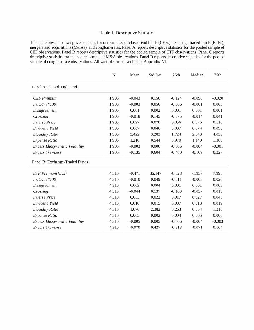
Table 1. Descriptive Statistics

This table presents descriptive statistics for our samples of closed-end funds (CEFs), exchange-traded funds (ETFs),

mergers and acquisitions (M&As), and conglomerates. Panel A reports descriptive statistics for the pooled sample of

CEF observations. Panel B reports descriptive statistics for the pooled sample of ETF observations. Panel C reports

descriptive statistics for the pooled sample of M&A observations. Panel D reports descriptive statistics for the pooled

sample of conglomerate observations. All variables are described in Appendix A1.

N Mean Std Dev 25th Median 75th

Panel A: Closed-End Funds

CEF Premium 1,906 -0.043 0.150 -0.124 -0.090 -0.020

InvCov (*100) 1,906 -0.003 0.056 -0.006 -0.001 0.003

Disagreement 1,906 0.001 0.002 0.001 0.001 0.001

Crossing 1,906 -0.018 0.145 -0.075 -0.014 0.041

Inverse Price 1,906 0.097 0.070 0.056 0.076 0.110

Dividend Yield 1,906 0.067 0.046 0.037 0.074 0.095

Liquidity Ratio 1,906 3.422 3.283 1.724 2.543 4.038

Expense Ratio 1,906 1.216 0.544 0.970 1.140 1.380

Excess Idiosyncratic Volatility 1,906 -0.003 0.006 -0.006 -0.004 -0.001

Excess Skewness 1,906 -0.135 0.604 -0.480 -0.109 0.227

Panel B: Exchange-Traded Funds

ETF Premium (bps) 4,310 -0.471 36.147 -8.028 -1.957 7.995

InvCov (*100) 4,310 -0.010 0.049 -0.011 -0.003 0.020

Disagreement 4,310 0.002 0.004 0.001 0.001 0.002

Crossing 4,310 -0.044 0.137 -0.103 -0.037 0.019

Inverse Price 4,310 0.033 0.022 0.017 0.027 0.043

Dividend Yield 4,310 0.016 0.015 0.007 0.013 0.019

Liquidity Ratio 4,310 1.076 2.382 0.263 0.654 1.216

Expense Ratio 4,310 0.005 0.002 0.004 0.005 0.006

Excess Idiosyncratic Volatility 4,310 -0.005 0.005 -0.006 -0.004 -0.003

Excess Skewness 4,310 -0.070 0.427 -0.313 -0.071 0.164

Table 1. Continued.

N Mean Std Dev 25th Median 75th

Panel C: Mergers and Acquisitions

Combined Announcement Day Return 405 0.021 0.070 -0.016 0.011 0.055

Acquirer Announcement Day Return 405 -0.013 0.070 -0.049 -0.010 0.017

Target Announcement Day Return 405 0.227 0.260 0.093 0.187 0.312

InvCov (*100) 405 0.002 0.255 -0.030 0.000 0.025

Disagreement 405 0.002 0.004 0.000 0.001 0.002

Crossing 405 -0.019 0.605 -0.500 0.000 0.462

Acquirer Characteristics:

Acquirer Market Capitalization 405 27,740 48,391 1,838 6,223 25,489

Acquirer Market-to-Book Ratio 405 3.498 3.257 1.624 2.366 4.155

Acquirer ROA 405 0.094 0.084 0.041 0.090 0.145

Acquirer Leverage 405 0.563 0.217 0.416 0.565 0.717

Acquirer Operating Cash Flow 405 0.105 0.078 0.059 0.107 0.153

Acquirer ATP Index 405 2.208 1.121 1.889 2.000 3.000

Target Characteristics:

Target Market Capitalization 405 2,623 5,105 4,029 9,896 22,340

Target Market-to-Book Ratio 405 3.984 2.849 1.489 2.233 3.403

Target ROA 405 0.052 0.131 0.015 0.064 0.115

Target Leverage 405 0.523 0.251 0.298 0.537 0.724

Target Operating Cash Flow 405 0.073 0.115 0.027 0.080 0.135

Target ATP Index 405 2.077 1.308 1.581 2.000 2.272

Panel D: Conglomerates

Diversification Premium 14,792 -0.149 0.750 -0.577 -0.175 0.244

Disagreement 14,792 0.008 0.025 0.001 0.002 0.005

Number of Segments 14,792 2.358 0.658 2.000 2.000 3.000

Total Assets 14,792 5,809 31,853 93.9 450.6 2,402.1

Leverage 14,792 0.193 0.162 0.050 0.172 0.295

Profitability 14,792 0.051 0.192 0.028 0.075 0.127

Investment Ratio 14,792 0.072 0.108 0.022 0.039 0.073

Excess Idiosyncratic Volatility 14,792 -0.005 0.066 -0.037 -0.014 0.013

Excess Skewness 14,792 -0.012 0.646 -0.427 -0.031 0.379

Table 2. Embedded Belief Crossing and Closed-End Fund Discounts

This table reports coefficient estimates from pooled OLS regressions of quarterly CEF premia on a measure of investor

disagreement and belief crossing across the CEF’s holdings. The dependent variable is the difference between the

CEF’s market price and the CEF’s NAV, divided by the CEF’s NAV [%]. We construct InvCov as follows: For each

stock pair involving securities of the CEF’s top-ten holdings, we compile a list of brokerage houses that cover both

firms and we compute the Spearman rank correlation in earnings forecasts between these two firms; we also compute

the forecast dispersion for each of the two firms. PairwiseCov is the product of the Spearman rank correlation and the

average forecast dispersion. We aggregate PairwiseCov to InvCov as the portfolio-weighted average PairwiseCov

across all stock pairs, multiplied by negative one. A large positive realization of InvCov suggests a high level of

embedded belief crossing. In Columns 2 and 3, we augment InvCov with (1-IO) and with (1-IO) * SI, respectively,

where IO is the residual institutional ownership and SI is short interest. We describe how we construct the remaining

variables in Appendix A1. All independent variables are normalized to have a standard deviation of one. We include

fund- and year-quarter-fixed effects. T-statistics are reported in parentheses and are based on standard errors clustered

by both fund and year-quarter. Statistical significance at the 10%, 5%, and 1% levels is denoted by *, **, and ***,

respectively.

Baseline

InvCov

(1)

Embed IO

into InvCov

(2)

Embed IO and SI

into InvCov

(3)

InvCov -0.491***

(-2.68)

-0.567***

(-2.61)

-0.499**

(-2.48)

Disagreement 0.388

(0.91)

0.569

(1.26)

0.478

(1.14)

Crossing

0.034

(0.19)

0.085

(0.49)

0.010

(0.05)

IO 0.675

(1.35)

0.711

(1.38)

SI -0.769

(-1.48)

Inverse Pricepos -1.017

(-0.59)

-0.955

(-0.55)

-0.933

(-0.54)

Inverse Priceneg -4.712***

(-2.61)

-4.669***

(-2.60)

-4.722***

(-2.63)

Dividend Yieldpos 1.554

(1.54)

1.517

(1.50)

1.519

(1.50)

Dividend Yieldneg -0.130

(-0.26)

-0.125

(-0.25)

-0.045

(-0.09)

Liquidity Ratio 1.372***

(2.70)

1.286**

(2.55)

1.400***

(2.75)

Expense Ratio 0.925

(1.07)

0.884

(1.06)

0.945

(1.11)

Excess Idiosyncratic Volatility 0.526

(0.75)

0.504

(0.71)

0.426

(0.61)

Excess Skewness 0.135

(1.23)

0.145

(1.31)

0.140

(1.36)

# Obs. 1,906 1,906 1,906

Adj. R2 0.843 0.844 0.844

Table 3. Embedded Belief Crossing and Exchange-Traded Fund Discounts

This table reports coefficient estimates from pooled OLS regressions of quarterly ETF premia on a measure of investor

disagreement and belief crossing across the ETF’s holdings. The dependent variable is the difference between the

ETF’s market price and the ETF’s NAV, divided by the ETF’s NAV [%]. We construct InvCov as follows: For each

stock pair involving securities of the ETF’s top-ten holdings, we compile a list of brokerage houses that cover both

firms and we compute the Spearman rank correlation in earnings forecasts between these two firms; we also compute

the forecast dispersion for each of the two firms. PairwiseCov is the product of the Spearman rank correlation and the

average forecast dispersion. We aggregate PairwiseCov to InvCov as the portfolio-weighted average PairwiseCov

across all stock pairs, multiplied by negative one. A large positive realization of InvCov suggests a high level of

embedded belief crossing. In Columns 2 and 3, we augment InvCov with (1-IO) and with (1-IO) * SI, respectively,

where IO is the residual institutional ownership and SI is short interest. We describe how we construct the remaining

variables in Appendix A1. All independent variables are normalized to have a standard deviation of one. We include

fund- and year-quarter-fixed effects. T-statistics are reported in parentheses and are based on standard errors clustered

by both fund and year-quarter. Statistical significance at the 10%, 5%, and 1% levels is denoted by *, **, and ***,

respectively.

Baseline

InvCov

(1)

Embed IO

into InvCov

(2)

Embed IO and SI

into InvCov

(3)

InvCov

-1.465**

(-2.24)

-1.697**

(-2.41)

-1.744**

(-2.54)

Disagreement 0.582

(0.47)

0.586

(0.58)

-0.259

(-0.42)

Crossing

0.505

(1.04)

0.576

(1.24)

0.520

(1.09)

IO

-0.249

(-0.19)

-0.163

(-0.13)

SI

2.800**

(1.98)

Inverse Pricepos 3.683

(0.83)

3.758

(0.86)

3.816

(0.90)

Inverse Priceneg -10.344**

(-2.02)

-10.274**

(-2.03)

-10.211**

(-2.08)

Dividend Yieldpos 1.822

(1.30)

1.822

(1.30)

1.742

(1.26)

Dividend Yieldneg -4.561***

(-3.22)

-4.538***

(-3.21)

-4.624***

(-3.32)

Liquidity Ratio

-1.896

(-1.12)

-1.874

(-1.11)

-2.117

(-1.29)

Expense Ratio 2.357

(0.64)

2.363

(0.64)

2.142

(0.57)

Excess Idiosyncratic Volatility

-1.875

(-0.71)

-1.903

(-0.72)

-1.719

(-0.66)

Excess Skewness

0.583

(0.64)

0.597

(0.65)

0.597

(0.66)

# Obs. 4,310 4,310 4,310

Adj. R2 0.372 0.372 0.373

Table 4. Embedded Belief Crossing and Exchange-Traded Fund Flows

This table reports coefficient estimates from pooled OLS regressions of monthly ETF flows on a measure of investor

disagreement and belief crossing. The dependent variable is the percentage change in the number of shares outstanding

of the ETF. The independent variables are as in Table 3, but now represent quarterly changes (rather than levels). All

independent variables are normalized to have a standard deviation of one. We include year-quarter-fixed effects (we

no longer include fund-fixed effects since all of our variables are now first-differenced). T-statistics are reported in

parentheses and are based on standard errors clustered by both fund and year-quarter. Statistical significance at the

10%, 5%, and 1% levels is denoted by *, **, and ***, respectively.

Baseline

InvCov

(1)

Embed IO

into InvCov

(2)

Embed IO and SI

into InvCov

(3)

∆InvCov

-0.380***

(-3.05)

-0.440**

(-2.56)

-0.405***

(-2.70)

∆Disagreement

-0.434**

(-2.48)

-0.426**

(-2.36)

0.068

(0.83)

∆Crossing

0.165

(1.40)

0.153

(1.30)

0.393**

(2.35)

∆IO -0.133

(-0.08)

-0.098

(-0.58)

∆SI

0.134

(0.76)

∆Dividend Yield 0.437*

(1.75)

0.445*

(1.76)

0.447*

(1.75)

∆Liquidity Ratio

-1.277***

(-8.54)

-1.278***

(-8.50)

-1.279***

(-8.51)

∆Expense Ratio -0.024

(-0.30)

-0.035

(-0.44)

-0.038

(-0.49)

∆Excess Idiosyncratic Volatility

-0.517***

(-4.71)

-0.502***

(-4.68)

-0.444***

(-3.83)

(0.68) ∆Excess Skewness

0.057

(0.32)

0.059

(0.33)

0.049

(0.27)

Lagged Returns Yes Yes Yes

Lagged Flows Yes Yes Yes

# Obs. 8,092 8,092 8,092

Adj. R2 0.026 0.025 0.025

Table 5. Embedded Belief Crossing and Combined M&A Announcement Day Returns

This table reports coefficient estimates from regressions of combined M&A announcement day returns on a measure

of investor disagreement and belief crossing about the acquirer and the target. The dependent variable is the average

cumulative abnormal return [-1,+1] across the acquirer and the target where t=0 is the day (or the ensuing trading day)

of the M&A announcement, weighted by the acquirer’s and the target’s market capitalization in the month prior to the

announcement [%].We construct InvCov as follows: We compile a list of brokerage houses that cover both the acquirer

and the target and we compute the Spearman rank correlation in earnings forecasts between these two firms; we also

compute the forecast dispersion for each of the two firms. InvCov is the product of the Spearman rank correlation and

the average forecast dispersion, multiplied by negative one. A large positive realization of InvCov suggests a high

level of embedded belief crossing. In Panels B and C, we augment InvCov with (1-IO) and with (1-IO) * SI,

respectively, where IO is the residual institutional ownership and SI is short interest. We describe how we construct

the remaining variables in Appendix A1. All independent variables are normalized to have a standard deviation of

one. We include year-fixed effects. T-statistics are reported in parentheses and are based on standard errors clustered

by year. Statistical significance at the 10%, 5%, and 1% levels is denoted by *, **, and ***, respectively.

Baseline

InvCov

(1)

Embed IO

into InvCov

(2)

Embed IO and SI

into InvCov

(3)

InvCov -1.713***

(-4.72)

-1.380***

(-3.44)

-1.057***

(-2.71)

Disagreement -0.763**

(-2.11)

-0.373

(-0.99)

-0.428

(-1.06)

Crossing

0.215

(0.61)

0.276

(0.72)

-0.026

(-0.07)

IO -0.408

(-0.91)

-0.520

(-1.16)

SI 0.385

(0.86)

Acquirer Characteristics:

ln(Acquirer Market Cap)

-1.382

(-1.42)

-1.134

(-1.09)

-0.962

(-0.89)

Acquirer Market-to-Book Ratio

0.618

(1.51)

0.590

(1.41)

0.570

(1.36)

Acquirer ROA

0.321

(0.60)

0.334

(0.61)

0.383

(0.69)

Acquirer Leverage

-0.081

(-0.16)

0.006

(0.01)

-0.064

(-0.12)

Acquirer Operating Cash Flow -0.723

(-1.22)

-0.521

(-0.96)

-0.550

(-1.00)

Acquirer ATP Index -0.131

(-0.27)

-0.148

(-0.30)

-0.116

(-0.23)

Table 5. Continued.

Baseline

InvCov

(1)

Embed IO

into InvCov

(2)

Embed IO and SI

into InvCov

(3)

Target Characteristics:

ln(Target Market Cap)

0.050

(0.06)

0.108

(0.13)

0.061

(0.07)

Target Market-to-Book Ratio

-0.416

(-1.12)

-0.430

(-1.13)

-0.454

(-1.19)

Target ROA

1.284**

(2.13)

1.462**

(2.39)

1.437**

(2.34)

Target Leverage 0.322

(0.70)

0.334

(0.72)

0.377

(0.81)

Target Operating Cash Flow

-1.333**

(-2.37)

-1.515***

(-2.66)

-1.529***

(-2.67)

Target ATP Index 0.780

(0.79)

0.667

(0.67)

0.697

(0.69)

Deal Characteristics:

Relative Size

-1.596**

(-2.12)

-1.470*

(-1.92)

-1.394*

(-1.82)

Combined Idiosyncratic Volatility

0.415

(0.78)

0.351

(0.64)

0.349

(0.63)

Combined Skewness -0.123

(-0.35)

-0.095

(-0.26)

-0.119

(-0.33)

Tender Offer -0.650

(-0.61)

-0.727

(-0.67)

-0.662

(-0.61)

Hostile Offer 2.249

(0.73)

2.434

(0.77)

2.414

(0.76)

Competing Offers 1.650

(0.83)

1.721

(0.85)

1.908

(0.94)

Cash Only 2.964***

(3.41)

2.784***

(3.14)

2.763***

(3.08)

Stock Only -0.551

(-0.62)

-0.616

(-0.68)

-0.776

(-0.85)

Same Industry 0.600

(0.81)

0.721

(0.95)

0.756

(0.99)

# Obs. 405 405 405

Adj. R2 0.314 0.294 0.288

Table 6. Investor Disagreement and Conglomerates

This table reports coefficient estimates from regressions of annual diversification premia on a measure of disagreement

about the conglomerate’s underlying segments. The dependent variable is the difference between the conglomerate’s

market-to-book ratio (MB) and its imputed MB, divided by the conglomerate’s imputed MB [%]. Imputed MB and

Disagreement are the sales-weighted average two-digit-SICMB and the sales-weighted average two-digit-SIC price-

scaled earnings forecast dispersion across the conglomerate’s segments as of t. We use information in June of calendar

year t to compute the market value of equity and we use accounting data from the fiscal year ending in the previous

calendar year t-1 to compute the book value of equity. Earnings forecasts are for annual earnings with fiscal year

ending in calendar year t-1. We describe how we construct the remaining variables in Appendix A1. All independent

variables are normalized to have a standard deviation of one. In Column (1), we estimate a pooled OLS regression

with year-fixed effects; t-statistics are computed using standard errors clustered by both firm and year. In Column (2),

we estimate annual Fama-MacBeth (1973) regressions; t-statistics are based on Newey-West (1987) standard errors

with one lag and are reported in parentheses. The Adj. R2 in Column (2) is the average Adj. R2 of the cross-sectional

regressions. Statistical significance at the 10%, 5%, and 1% levels is denoted by *, **, and ***, respectively.

(1) (2)

Disagreement -0.043***

(-2.92)

-0.069***

(-6.10)

Number of Segments -0.014

(-1.08)

-0.015***

(-2.90)

ln(TotalAssets) -0.719***

(-9.20)

-0.849***

(-16.98)

ln(TotalAssets)2 0.621***

(7.79)

0.732***

(15.92)

Leverage 0.072***

(4.69)

0.800***

(7.14)

Profitability 0.015

(1.11)

0.026***

(3.37)

Investment Ratio 0.024*

(1.89)

0.031***

(3.42)

Excess Idiosyncratic Volatility 0.059***

(3.64)

0.048***

(3.61)

Excess Skewness 0.021***

(3.19)

0.019***

(2.86)

# Obs. 14,792 31

Adj. R2 0.075 0.086