Policy Research Working Paper 7440

The Impact of Violence on Individual Risk Preferences

Evidence from a Natural Experiment

Pamela Jakiela Owen Ozier

Development Research GroupHuman Development and Public Services TeamOctober 2015

WPS7440P

ublic

Dis

clos

ure

Aut

horiz

edP

ublic

Dis

clos

ure

Aut

horiz

edP

ublic

Dis

clos

ure

Aut

horiz

edP

ublic

Dis

clos

ure

Aut

horiz

ed

Produced by the Research Support Team

Abstract

The Policy Research Working Paper Series disseminates the findings of work in progress to encourage the exchange of ideas about development issues. An objective of the series is to get the findings out quickly, even if the presentations are less than fully polished. The papers carry the names of the authors and should be cited accordingly. The findings, interpretations, and conclusions expressed in this paper are entirely those of the authors. They do not necessarily represent the views of the International Bank for Reconstruction and Development/World Bank and its affiliated organizations, or those of the Executive Directors of the World Bank or the governments they represent.

Policy Research Working Paper 7440

This paper is a product of the Human Development and Public Services Team, Development Research Group. It is part of a larger effort by the World Bank to provide open access to its research and make a contribution to development policy discussions around the world. Policy Research Working Papers are also posted on the Web at http://econ.worldbank.org. The authors may be contacted at oozier@worldbank.org.

This study estimates the impact of Kenya’s post-election violence on individual risk preferences. Because the crisis interrupted a longitudinal survey of more than five thou-sand Kenyan youth, this timing creates plausibly exogenous variation in exposure to civil conflict by the time of the survey. The study measures individual risk preferences using hypothetical lottery choice questions, which are validated by showing that they predict migration and

entrepreneurship in the cross-section. The results indi-cate that the post-election violence sharply increased individual risk aversion. Immediately after the crisis, the fraction of subjects who are classified as either risk neutral or risk loving dropped by roughly 26 percent. The findings remain robust to an IV estimation strategy that exploits random assignment of respondents to waves of surveying.

The Impact of Violence on Individual Risk Preferences:

Evidence from a Natural Experiment

Pamela Jakiela and Owen Ozier∗

JEL codes: C91, C93, D01, D74, D81

Keywords: risk preferences, civil conflict, natural experiment

∗Jakiela: University of Maryland and IZA, pjakiela@umd.edu; Ozier: Development Research Group, The WorldBank, oozier@worldbank.org. We are grateful to the staff at IPA-Kenya for their assistance and support, and toMichael Callen, Marcel Fafchamps, Jonas Hjort, Diego Garrido Martin, Ted Miguel, Anja Sautmann, and Waly Wanefor helpful comments. All errors are our own.

1 Introduction

Armed conflict is a source of untold human suffering. Since 1989, more than one million people

have been killed in civil and interstate conflicts (Pettersson and Wallensteen 2015). The majority of

these episodes are civil wars in low- and middle-income countries; because the scourge of war falls

disproportionately on the poorest nations, armed conflict also perpetuates disparities in human

and economic development among the living.

The short-term costs of civil conflict are obvious: in addition to the lives lost, war damages

or destroys physical capital and deters investment. There is also evidence that war and violence

limit the accumulation of human capital (Blattman and Annan 2010) and erode trust (Nunn and

Wantchekon 2011). This has led some scholars to refer to civil war as “development in reverse”

(Collier, Elliott, Hegre, Hoeffler, Reynal-Querol, and Sambanis 2003). Yet, though the short-

term human and economic costs of conflict are indisputable, many conflict-affected countries —

Rwanda and Uganda, for example — have experienced extremely rapid growth in the wake of

civil war, and a number of recent papers have challenged the notion that conflict leads to slower

growth and development over the long-term (cf. Miguel and Roland 2011). In fact, several studies

have found that exposure to civil conflict increases political engagement (Bellows and Miguel 2009,

Blattman 2009), enhances cooperation and pro-sociality (Voors, Nillesen, Verwimp, Bulte, Lensink,

and Van Soest 2012, Bauer, Cassar, Chytilova, and Henrich 2013), and makes people more willing

to bear profitable risks (Voors, Nillesen, Verwimp, Bulte, Lensink, and Van Soest 2012, Callen,

Isaqzadeh, Long, and Sprenger 2014).

These studies share a common empirical approach. First, they take seriously the idea that

exposure to conflict is endogenous, and employ a variety of strategies designed to isolate plausibly

exogenous variation in victimization and involvement in violence. Second, given their focus on

within-conflict variation in exposure and victimization, these papers empirically frame civilians who

lived through civil war but were not victimized (or were less exposed to violence) as a comparison

group. This strategy enhances the credibility of the estimated treatment effects, but has an obvious

drawback: this approach can generate credible estimates of the marginal impact of greater conflict

victimization or exposure, but cannot be used to assess the overall impact of conflict unless one

2

assumes that violence has no impact on the relatively less victimized. If everyone who lives through

a period of conflict — regardless of their victim status — is affected, estimates of the marginal

impact of greater conflict exposure may present a biased assessment of the overall social cost of

violence.

In this paper, we estimate the impact of a specific episode of civil conflict, Kenya’s post-

election crisis, on the risk preferences of a broad sample of young adults who lived through it. The

post-election crisis was a months-long period of protests, rioting, and ethnic violence that began

immediately after a disputed presidential election. The election, in which Raila Odinga challenged

incumbent Mwai Kibaki, took place on December 27, 2007. Amidst allegations of electoral fraud by

observers, and after three days of uncertainty following the national polls, the incumbent president

was both declared the winner and sworn into office on December 30, 2007. Ethnic tensions rose,

and rioting ensued. The following two months of civil conflict left more than a thousand people

dead and hundreds of thousands more internally displaced. The crisis largely ended when, on

February 28, 2008, the two candidates signed a power-sharing agreement.1

We estimate the impact of Kenya’s post-election violence on individual risk preferences, which

we measure using lottery choice questions embedded in a longitudinal survey. The Kenyan Life

Panel Survey (hereafter KLPS2) is a survey of more than 5,000 young adults who were enrolled in

rural primary schools in 1998. The second round of the survey was administered between August of

2007 and December of 2009. 1,180 respondents (23.3 percent) were interviewed prior to the crisis,

while the remainder were surveyed after experiencing the period of civil conflict. Thus, Kenya’s

post-election violence interacted with the timing of the survey to create a natural experiment in

exposure to conflict.

We employ two complementary identification strategies to estimate the impact of the crisis on

risk aversion. First, we estimate the impact of the crisis in straightforward linear and nonlinear

frameworks, using several strategies to control for any time trends or seasonal shocks. Second, we

exploit the fact that survey respondents were randomly assigned to one of two waves of interviews;

Kenya’s election crisis interrupted the first wave of surveys, allowing us to instrument for conflict

1 This description of Kenya’s 2007-2008 post-election crisis draws upon several sources: World Bank (2006), WorldBank (2008), World Bank (2009), World Bank (2010a), World Bank (2010b), World Bank (2011), World Bank (2012),Van Praag (2010), Waki (2008), Hjort (forthcoming), McCrummen (2007), BBC (2008a), and BBC (2008b).

3

exposure (pre-survey) using the randomly-assigned survey waves. Both approaches yield similar

results: we find that Kenya’s post-election crisis had a large and significant positive impact on indi-

vidual risk aversion. Specifically, the crisis led to an 11 percentage point increase in the likelihood

that a subject always chose the safest, lowest expected value alternative (i.e. lottery) available —

this effect constitutes more than an 80 percent increase in the rate of extreme risk aversion. We

also observe a 5.7 percentage point (or roughly 26 percent) decrease in the fraction of subjects

who are classified as either risk neutral or risk loving. Such substantial impacts highlight an im-

portant channel through which civil conflict might affect growth and development: increased risk

aversion might lead individuals in post-conflict settings to avoid high-risk, high-return activities

(e.g. entrepreneurship) that contribute to economic growth.

The key strength of our study is that we are able to estimate the impact of civil conflict on

the risk preferences of the general population, as opposed to the specific (marginal) effect of being

victimized or more exposed to violence. Very few KLPS2 respondents were themselves victims of

violence during the unrest: more than three quarters of respondents were temporarily deprived

of basic necessities because it was not safe to visit markets or other public places, but less than

4 percent indicated that anyone in their household was physically assaulted during the crisis.

Thus, KLPS2 respondents experienced the conflict, but were not, by and large, among the most

impacted Kenyans; they therefore provide an important window into the impacts of civil conflicts

on the preferences of the general population.

Our results differ from several recent studies. For example, Voors, Nillesen, Verwimp, Bulte,

Lensink, and Van Soest (2012) find that greater exposure to violence leads to an increase in risk-

seeking behavior, while Callen, Isaqzadeh, Long, and Sprenger (2014) find that priming subjects

with recollections of violent events increases their risk tolerance in situations involving only uncer-

tainty (but also increases their certainty premia). However, these differing results can be reconciled

by the difference in estimands, for example, if those who narrowly escape being exposed to violence

or victimized become more risk averse. Our aim in this paper is to estimate the overall impact of

violence on the population as a whole; doing so, we may not find the same effect. Understanding

these overall impacts is of critical importance as we seek to characterize the ways that conflict may

change a country’s overall growth trajectory.

4

This paper contributes to several strands of literature. First, most obviously, we add to the

evidence on the impacts of conflict. As discussed above, this literature has expanded rapidly

in recent years as increasingly high-quality micro data from post-conflict settings has become

available.2 Second, we contribute to a growing body of evidence that individual preferences, one

of the key determinants of individual behavior in all economic domains, are not as immutable as

has long been assumed (cf. Stigler and Becker 1977); instead, individual preferences appear to be

shaped by life experiences. For example, Malmendier and Nagel (2011) and Fisman, Jakiela, and

Kariv (2015) show that exposure to economic downturns makes people more risk averse and more

efficiency-focused, respectively; while Eckel, El-Gamal, and Wilson (2009), Cameron and Shah

(2013), and Hanaoka, Shigeoka, and Watanabe (2015) estimate the impact of natural disasters on

individual risk preferences (and arrive at different conclusions). As discussed above, several papers

(cf. Voors, Nillesen, Verwimp, Bulte, Lensink, and Van Soest 2012) have estimated the impact

of conflict on the preferences of those most affected, but, to our knowledge, no work to date has

estimated the impact of violence on the risk preferences of the general population.

Finally, our study contributes to the growing body of evidence documenting the validity and

predictive power of laboratory and lab-style measures of individual preferences. Though some

scholars have questioned whether individual decisions in choice experiments predicts behavior out-

side of the lab (cf. Levitt and List 2007, Voors, Turley, Kontoleon, Bulte, and List 2012), numerous

studies document the explanatory power of experimental measures of risk, time, and social prefer-

ences. For example, Liu (2013) and Liu and Huang (2013) show that experimental measures of risk

preferences predict the crop choice and investment decisions of Chinese farmers. In the domain of

time preferences, Meier and Sprenger (2012) show that experimental measures of patience predict

creditworthiness. Fisman, Jakiela, and Kariv (2014) show that experimental measures of equality-

efficiency tradeoffs predict the voting behavior of adult Americans, while Fisman, Jakiela, Kariv,

and Markovits (2015) show that the same measure predicts the post-graduation career choices of

law students. Jing (2015) shows that experimental measures of fair-mindedness predict medical

students’ choices regarding field of specialization. To date, the majority of work linking choices

2Humphreys and Weinstein (2006), Bellows and Miguel (2009), and Blattman and Annan (2010) are prominentexamples. See Blattman and Miguel (2010) for discussion.

5

in decision experiments to behavior outside the lab has used incentivized measures of individual

preferences, but there are notable exceptions (cf. Ashraf, Karlan, and Yin 2006). Existing evi-

dence suggests the use of incentives shifts individual responses toward greater risk aversion (cf.

Camerer and Hogarth 1999, Holt and Laury 2002), leading many to question the broad applica-

bility of hypothetical approaches to risk preference elicitation. We contribute to this literature

by demonstrating that hypothetical measures of risk preferences, interpreted as an ordinal index

of risk tolerance, predict real world behaviors in an internally consistent way. In particular, our

measure of risk preferences is associated with real-world behaviors that involve risk: migration and

entrepreneurship.

The rest of this paper is organized as follows. In Section 2, we describe the KLPS2 data collec-

tion effort and Kenya’s post-election crisis. In Section 3, we describe our measure of risk preferences

and assess the extent to which our hypothetical lottery choice questions predict behaviors likely

to depend on risk aversion. In Section 4, we explain our analytic approach and present our main

results. Section 5 concludes.

2 Research Design

2.1 The Kenyan Life Panel Survey

We measure the risk preferences of a large and heterogeneous sample of young Kenyans by em-

bedding a series of non-incentivized decision problems in the second round of the Kenyan Life

Panel Survey (KLPS2), which was administered to more than 5,000 individuals who were enrolled

in primary schools in Kenya’s Western Province in the late 1990s.3 KLPS2 was administered in

person, through one-on-one interviews, between August of 2007 and December of 2009. The survey

covers a broad range of topics including educational attainment, labor market and entrepreneurial

activities, household composition and wealth, migration, and fertility.

Our subject pool includes 5,049 Kenyan youths aged 14 to 31. Summary statistics characterizing

3KLPS2 was a long-term follow-up of the Primary School Deworming Project (PSDP) that was implemented inBusia District, in Kenya’s Western Province, between 1998 and 2001. All KLPS2 respondents were enrolled in publicprimary schools in the project area in 1998. See Miguel and Kremer (2004) for discussion of the PSDP and Baird,Blattman, Casaburi, Evans, Hamory, Kremer, Miguel, Ozier, Siegel, Wafula, and Yeh (2007) for a description of theKLPS data collection effort.

6

our sample are reported in the Online Appendix. 49.0 percent of subjects are female. As of 2007,

subjects had completed an average of 8.5 years of schooling; 69.6 percent had completed primary

school, and 14.4 percent had completed secondary school. 23.2 percent of subjects were still enrolled

in school at the time that they were surveyed.

2.2 Kenya’s Post-Election Crisis

The 2008 post-election crisis was a period of violence and political instability following the Kenyan

presidential election of December 27, 2007. The two leading candidates in the election were Raila

Odinga (the son of Kenya’s first vice president), and the incumbent president, Mwai Kibaki (himself

a former vice president). For several months preceding the election, opinion polls placed the

opposition candidate, Odinga, ahead of Kibaki (World Bank 2008, Munene and Otieno 2007). As

election day neared, the polling gap between Odinga and Kibaki narrowed to what, in some polls,

appeared to be a statistical dead heat (World Bank 2008, Agina 2007, Otieno 2007, Standard Team

2007). At the time of the elections, both international observers and members of the opposition

made allegations of electoral irregularities; however, after a few days, Kibaki was declared the

winner and sworn into office (World Bank 2008, Waki 2008, McCrummen 2007, BBC News 2007).

Opposition supporters organized protests; rioting and violent clashes with police ensued, and the

violence soon escalated and took on a strong ethnic dimension (World Bank 2008, World Bank

2010b, Van Praag 2010, Waki 2008, BBC News 2007). By the time Kibaki and Odinga signed

a power-sharing agreement at the end of February, 2008, more than one thousand people had

been killed, and hundreds of thousands had been internally displaced (World Bank 2008, World

Bank 2009, World Bank 2010a, World Bank 2012, BBC 2008a, BBC 2008b).

As discussed above, all KLPS2 respondents were residing in Busia District, in Kenya’s Western

Province near the Ugandan border, in 1998; 73 percent were still living in Busia District at the time

of the KLPS2 survey, and many others happened to be there during the post-election crisis (because

they had returned to their family homes to celebrate the Christmas holiday or to vote). As a result,

most were spared the worst of the post-election violence: though protests, riots, and assaults took

place throughout Kenya, the most affected areas were Rift Valley Province and the more urban

districts across the country. According to the official report of the Commission of Inquiry on Post

7

Election Violence, only 98 of the 1,133 conflict deaths occurred in Western Province (Waki 2008).

The majority of conflict deaths in Western Province occurred in districts that bordered Rift Valley

Province; only 9 deaths were documented in Busia District (Waki 2008). In addition, most KLPS2

respondents (90.0 percent) are members of the Luhya ethnic group, the majority ethnic group in

Western Province; as such, they were somewhat less likely to be singled out as clearly aligned

with either the incumbent Mwai Kibaki (a member of a different ethnic group) or the opposition

candidate Raila Odinga (a member of a third group).45 Thus, though KLPS2 survey respondents

lived through the crisis, both their physical locations and their ethnic identities helped to shield

most of them from the worst of the violence.

This pattern is borne out in the data. The second wave of the survey included questions on

exposure to violence during the post-election crisis; it documents the fact that very few respondents

were, themselves, the victims of physical attacks.6 76.3 percent of KLPS2 Wave 2 respondents

reported that the crisis prevented them from going to local markets to obtain basic necessities,

but only 3.7 percent indicated that someone in their household was physically assaulted during

the crisis. Similarly low numbers of respondents had property stolen (5.8 percent) or burned (2.1

percent) during the crisis. Thus, though many of our subjects were directly affected by the crisis

because businesses and markets were closed and people were confined to their homes during periods

of rioting and insecurity, relatively few were, themselves, victims of violence. Our estimates should

therefore be seen as both a lower bound on the impact of civil conflict on risk preferences, and

a natural complement to studies which estimate the impact of violence on those individuals and

households who were most victimized.

3 Measuring Risk Preferences

We elicit risk preferences by confronting survey respondents with a series of hypothetical decision

problems; each decision was a choice between two or three lotteries involving two equally likely

4Western Province was an opposition stronghold, and Raila Odinga received 64.6 percent of the votes cast therein the presidential election; thus, individuals perceived as likely supporters of the incumbent were the most at risk.

5We thank the World Bank’s Kenya Country Office for guidance on wording.6As discussed above, KLPS2 respondents were randomly assigned to one of two waves of surveying. The post-

election violence interrupted the first wave of surveying. The additional survey were included only in Wave 2, soresponses can be seen as representative of the entire respondent population.

8

potential payoffs. The sequence of decision problems was designed to start with choices that were

extremely simple and to build slowly toward more complicated choice problems. For example,

the first decision problem involved a choice between a degenerate lottery which paid 100 Kenyan

shillings with certainty and a lottery involving a 50 percent chance of receiving 100 shillings and a

50 percent chance of receiving 120 shillings.7 In contrast, the final decision problem was a choice

between three non-degenerate lotteries.

This sequencing of choice problems from least to most complex served two purposes. First,

the gradual increase in complexity was intended to help address the concern that respondents

might not exert sufficient cognitive effort (for example, to calculate expected payoffs) when facing

non-incentivized choice problems.8 Respondents first considered options that could be evaluated

with minimal cognitive effort, easing into the process of evaluating the expected utility of financial

lotteries. Second, we wished to maximize the level of comprehension by subjects with low levels of

numeracy. For this reason, we also limited each decision problem to a maximum of three lottery

options, included only three easily understood probabilities (0, 0.5, and 1), and only considered

lotteries over financial gains (rather than losses).9 Our experimental instructions do not assume

any familiarity with probabilities, averages, or expected values; lotteries are explained in terms of

payoffs and uncertain but equally likely events.

When administering our experiment, survey enumerators began by presenting two practice de-

cision problems which introduced the structure of the lottery choice questions to the respondent.10

The first practice problem contained only degenerate lotteries — the respondent was asked to

choose between 100 Kenyan shillings and 150 shillings; the second practice problem introduced the

(non-degenerate) lottery concept in a setting with a clear “correct” answer: one lottery first-order

7The average US dollar value of 100 Kenyan shillings was 1.36 over the period during which the KLPS2 surveywas in the field, from August 2007 to December 2009.

8There is some debate about the extent to which non-incentivized lottery choice questions correctly measureindividual risk preferences. See Camerer (1995) for an overview, and Binswanger (1980) and Holt and Laury (2002)for seminal contributions. Existing evidence suggests that financial incentives induce greater risk aversion (Camererand Hogarth 1999). Embedding non-incentivized decision problems in surveys has nonetheless proven successful ina number of field settings in developing countries, when conducting incentivized experiments at scale is not feasible(cf. Callen, Isaqzadeh, Long, and Sprenger 2014).

9Our risk preference elicitation method builds on those of Binswanger (1980), Eckel and Grossman (2008), Barrand Genicot (2008), Tanaka, Camerer, and Nguyen (2010), and Liu (2013), among others, but differs in its exclusivefocus on extremely simple lottery structures and limited choice sets.

10Complete experimental instructions including images of the cards depicting lottery choice questions are includedin the Online Appendix.

9

stochastically dominated the other, and both involved risk. Enumerators asked respondents to

choose between the lotteries presented in the practice decision problems, and then followed a script

which made sure that each respondent fully understood the nature of the choices they were facing.

After completing the practice decision problems, each subject made six choices between lotteries

which differed in riskiness. Each choice was presented on a laminated card which depicted either

two or three options. Like the practice problems, the first question (described above) provided a test

of monotonicity, allowing us to identify subjects who are either not expected utility maximizers (cf.

Andreoni and Sprenger 2010) or who simply could not grasp the nature of the choice problems. The

second decision problem offered an extremely simple test of risk preferences, and one which should

have been easily understood by almost all subjects: subjects were asked whether they preferred

to receive 100 shillings with certainty, or a 50 percent chance of 400 shillings. The remaining four

decision problems presented lottery choices of increasing complexity. Without any functional form

assumptions (but assuming subjects are maximizing a well-defined utility function), these decisions

can be used to classify subjects into risk preference categories: risk loving, risk neutral, moderately

risk averse, and most risk averse (always choosing the lotteries with the lowest expected value and

payoff spread). If we assume that consistent preferences can be represented by a utility function

of the constant relative risk aversion (CRRA) form, the risk cards were calibrated to distinguish a

wide range of coefficients in the neighborhood of 1.11 The payouts for the lotteries in all the choice

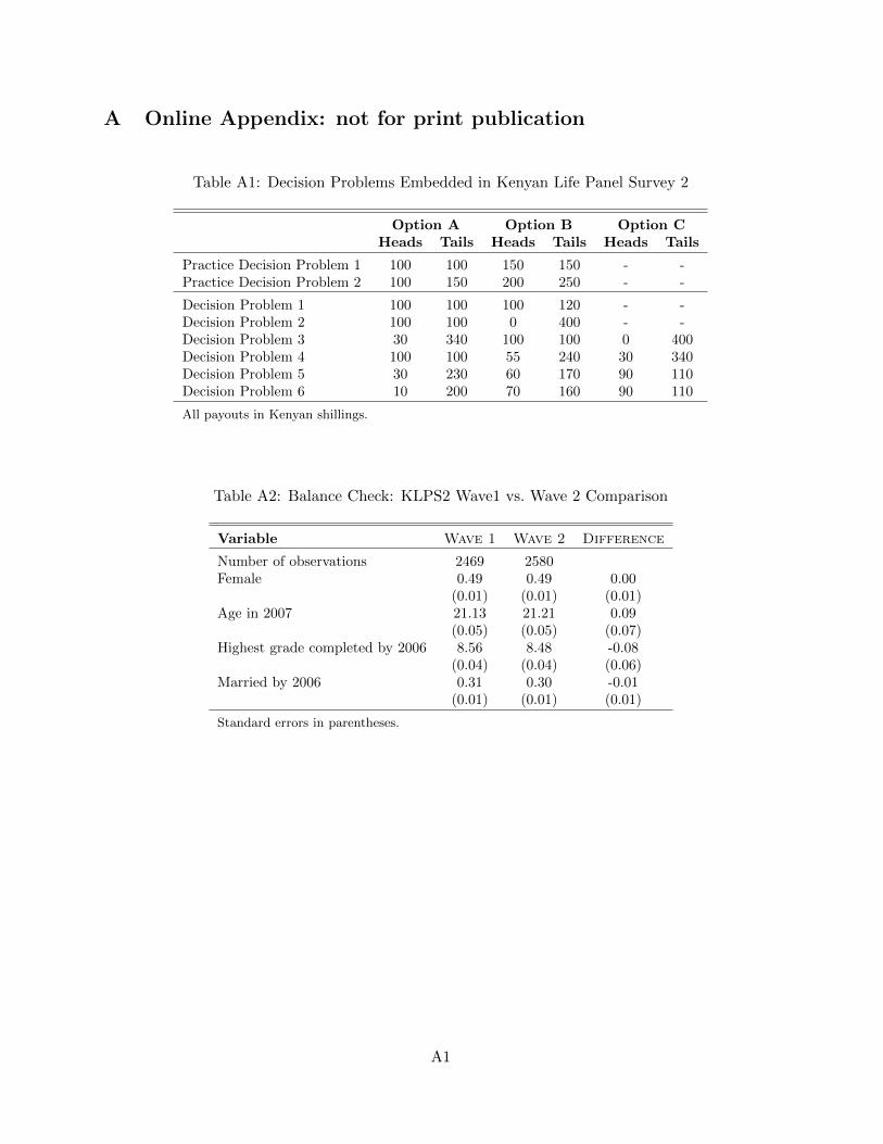
problems included in our experiment are described in the Online Appendix.

3.1 Individual Choices

Histograms of individual choices in all six decision problems are presented in the Online Appendix.

Very few respondents (only 4.14 percent) indicated that they preferred the degenerate lottery

which paid 100 Kenyan shillings with certainty to a non-degenerate lottery which paid either 100

or 120 Kenyan shillings, each with probability 0.5. We interpret this as evidence that most subjects

understood the nature of the decision problems, at least those that involved relatively simple payoff

11The CRRA utility function takes the form: u(x) = x1−ρ/(1 − ρ) where ρ indicates the level of risk aversion.Higher values of ρ indicate greater risk aversion. When ρ = 0, the agent is risk neutral; the indifference curvesrepresented by the CRRA utility function approach log utility as ρ approaches 1. Even if relative risk aversion isnot constant, constant relative risk aversion is a reasonable approximation over the relatively small range of payoffsconsidered in our experiment. The CRRA form is also used in this setting in Jakiela and Ozier (forthcoming).

10

calculations.12

Using data from the other five decision problems allows us to assign respondents to distinct risk

preference categories. We classify a subject as risk neutral if she always chose the lottery with

the highest expected value. We classify a subject as risk loving is she made risk neutral choices in

all except in the last decision problem, and then chose the lottery which paid 10 and 200 shillings

with equal probability over the lottery which paid 70 and 160 shillings with equal probability. We

classify those subjects who always opted for the lowest variance, lowest expected value lottery as

the most risk averse. The three categories most risk averse, risk neutral, and risk loving account

for 22.5, 2.4, and 15.7 percent of subjects, respectively.

Offering subjects a series of choices also allows us to test whether individual decisions are con-

sistent with a CRRA utility representation. There are 162 possible combinations of responses to

the last 5 lottery choice problems, only 10 of which are consistent with a CRRA utility repre-

sentation. 44.6 percent of subjects made choices which were consistent with the maximization of

a CRRA utility function. If subjects were choosing lotteries at random, only 6.2 percent would

make CRRA-consistent choices. However, only 4 percent of subjects made consistent choices that

were not classified as either most risk averse, risk neutral, and risk loving. Figure 1 presents the

fraction of respondents falling into each of five different categories: most risk averse, risk neutral,

risk loving, other types of consistent choices (suggesting intermediate levels of risk aversion), and

inconsistent choices. The figure demonstrates that patterns of choices which are inconsistent with

the maximization of a CRRA utility function occur substantially less frequently than we would

expect if subjects were selecting lotteries at random, but that only the first three types of consistent

12We also asked enumerators to indicate whether they believed that respondents fully understood the lotterychoice questions; these responses suggest that 99.6 percent of subjects fully comprehended the choices that they weremaking. There are, of course, several reasons that subjects who understood the decision problem might prefer adegenerate lottery to a stochastically dominant one involving risk. One possibility is that some respondents havepreferences which are not monotonic. Several non-expected utility models of risk preferences suggest that individualsmay prefer to avoid increases in payoff variance, even when the higher variance lottery stochastically dominates thelower variance alternative. For example, specifications of the non-linear probability weighting component of prospecttheory typically assume sub-additivity (Kahneman and Tversky 1979); the models of risk attitudes proposed byKosegi and Rabin (2006) and Andreoni and Sprenger (2010) are also consistent with a preference for the risk-free Option A over the stochastically dominant Option B. We interpret the overwhelming tendency to choose thestochastically dominant lottery as evidence against strongly non-monotonic preferences. One plausible interpretationof the observed choice patterns is that respondents have monotonic preferences which they implement with error(Hey and Orme 1994, Loomes 2005, Von Gaudecker, van Soest, and Wengstrom 2011, Choi, Kariv, Muller, andSilverman 2014).

11

behavior (extreme risk aversion, risk neutrality, and risk loving behavior) occur more frequently

than random choice would suggest.

3.2 Instrument Validity

To address concerns about the validity of hypothetical measures of risk aversion, we test whether

individual responses to our hypothetical lottery choice questions explain observed variation in

behaviors that we might expect to be driven (at least in part) by risk attitudes. We focus on two

such behaviors suggested by the literature: entrepreneurship (Schumpeter 1934, Schumpeter 1939,

Skriabikova, Dohmen, and Kriechel 2014) and migration in search of employment (Jaeger, Dohmen,

Falk, Huffman, Sunde, and Bonin 2010, Bryan, Chowdhury, and Mobarak 2014). Both of these

actions can be seen through the lens of risk tolerance: for an unemployed or underemployed young

adult residing in a rural area, operating one’s one business and migrating are two high risk but

potentially profitable strategies for improving one’s long-term income prospects. Both behaviors

are also relatively uncommon: only 12.4 percent of KLPS2 respondents were operating their own

business at the time of the survey, and only 3.5 percent had ever moved for a job or in search of

work.

To explore the association between these risky but potentially profitable activities and responses

to our lottery choice questions, we construct a simple index of risk tolerance: a count of the number

of times (out of five lottery choice questions) that a subject chose the riskiest and highest expected

value lottery.13 This index has two important strengths. First, it obviates the need to impose

functional form assumptions on the structure of risk preferences. In the decision problems included

in our study, all lotteries involving risk have two equally likely outcomes, and the highest expected

value lottery always has the highest variance and the lowest minimum payoff (i.e. the lowest payoff

in the bad state),14 so any parametric restriction that permits an ordering of utility functions in

13Focusing on the number of risky choices allows us to include those subjects whose decisions were not consistentwith a CRRA utility representation in our analysis. As discussed in Loomes (2005) and Choi, Kariv, Muller, andSilverman (2014), most subjects implement their choices with error — and we would expect relatively high levels oferror in our sample because of the relatively low level of formal schooling attained by our subjects. Importantly, ifthe likelihood of making consistent choices is associated with risk aversion, omitting the inconsistent subjects couldbias our results. However, all of our findings are robust to the omission of the inconsistent types from the analysis.

14The one exception to this is that the final lottery choice question included one alternative designed to distinguishbetween risk loving and risk neutral types. In this choice problem, we classify both the highest expected value lotteryand the highest variance lottery as risky, though we obtain similar results of we do not classify the highest expected

12

terms of risk aversion would predict that relatively more risk averse individuals will be less likely

to choose the highest variance lotteries. Second, constructing a measure of risk aversion that does

not rely on functional form assumptions allows us to use data from all subjects, including those

whose choices were not perfectly consistent with a specific utility representation.

We estimate probit regressions of indicators for operating one’s own business and having ever

migrated seeking work on our index of risk aversion: the number of times (out of five) that a

respondent chose the riskiest (highest expected value) lottery. Results are reported in Table 1. In

all specifications, the number of times a respondent opted for the riskiest lottery is significantly

associated with the likelihood of operating one’s own business or migrating for work. After con-

trolling for gender, education level, age, the month in which the survey took place, and the survey

enumerator who administered the lottery choice module, an additional risky choice is associated

with a 0.5 percentage point (4.3 percent) increase in the likelihood of operating a business and

a 0.2 percentage point (6.7 percent) increase in the likelihood of having ever migrated for work.

Given the many factors underlying occupational choices, we interpret these robust associations as

clear evidence that our lottery choice measure does predict outcomes associated with risk aversion

in the cross-section.

4 Analysis

4.1 Empirical Approach

We exploit the fact that Kenya’s post-election crisis occurred in the middle of the KLPS2 data

collection effort to estimate the impact of the violence on risk preferences. The KLPS2 survey was

launched in August of 2007, and 1,180 respondents were surveyed in 2007 prior to the elections.

The crisis led to a two-month suspension of survey activities, which resumed in March of 2008

and continued through the end of 2009. We employ two complementary identification strategies.

First, we estimate the impact of the crisis in a straightforward linear framework, controlling for

month-of-the-year fixed effects. In these specifications, we also include enumerator fixed effects

and controls for sociodemographic characteristics such as respondent age, educational attainment,

value lottery as a risky alternative.

13

and marital status that we expect to change over time.15 Thus, we estimate OLS regressions of

the form:

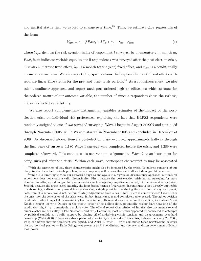
Yijm = α+ βPosti + δXi + ηj + λm + εijm (1)

where Yijm denotes the risk aversion index of respondent i surveyed by enumerator j in month m,

Posti is an indicator variable equal to one if respondent i was surveyed after the post-election crisis,

ηj is an enumerator fixed effect, λm is a month (of the year) fixed effect, and εijm is a conditionally

mean-zero error term. We also report OLS specifications that replace the month fixed effects with

separate linear time trends for the pre- and post- crisis periods.16 As a robustness check, we also

take a nonlinear approach, and report analogous ordered logit specifications which account for

the ordered nature of our outcome variable, the number of times a respondent chose the riskiest,

highest expected value lottery.

We also report complementary instrumental variables estimates of the impact of the post-

election crisis on individual risk preferences, exploiting the fact that KLPS2 respondents were

randomly assigned to one of two waves of surveying. Wave 1 began in August of 2007 and continued

through November 2008, while Wave 2 started in November 2008 and concluded in December of

2009. As discussed above, Kenya’s post-election crisis occurred approximately halfway through

the first wave of surveys: 1,180 Wave 1 surveys were completed before the crisis, and 1,289 were

completed afterward. This enables us to use random assignment to Wave 2 as an instrument for

being surveyed after the crisis. Within each wave, participant characteristics may be associated

15With the exception of age, these characteristics might also be impacted by the crisis. To address concerns aboutthe potential for a bad controls problem, we also report specifications that omit all sociodemographic controls.

16While it is tempting to view our research design as analogous to a regression discontinuity approach, our naturalexperiment does not create a valid discontinuity. First, because the post-election crisis halted surveying for morethan two months, sociodemographic characteristics such as age do jump discontinuously at the moment of the crisis.Second, because the crisis lasted months, the limit-based notion of regression discontinuity is not directly applicableto this setting; a discontinuity would involve choosing a single point in time during the crisis, and at any such point,data from this survey would not be immediately adjacent on both sides. Third, there is some evidence that neitherthe onset nor the conclusion of the crisis were, in fact, instantaneous and completely unexpected. Though oppositioncandidate Raila Odinga held a convincing lead in opinion polls several months before the election, incumbent MwaiKibabki caught up with Odinga in the month prior to the polling date, potentially raising fears that one of thecandidates might try to manipulate a close vote. The official report Commission of Inquiry also documents severalminor clashes in Rift Valley in late November and early December, most of which appeared be connected to attemptsby political candidates to rally support by playing off of underlying ethnic tensions and disagreements over landownership (Waki 2008). There was also a period of uncertainty in the wake of the crisis, between February 28, 2008,when the power-sharing agreement was signed, and April 12 when — after sometimes tense negotiations betweenthe two political parties — Raila Odinga was sworn in as Prime Minister and the new coalition government officiallytook power.

14

with how quickly an individual was surveyed — for example, subjects who were still residing with

their parents in their home villages might have been surveyed earlier because they were easier to

locate. However, random assignment to survey wave creates exogenous variation in exposure to

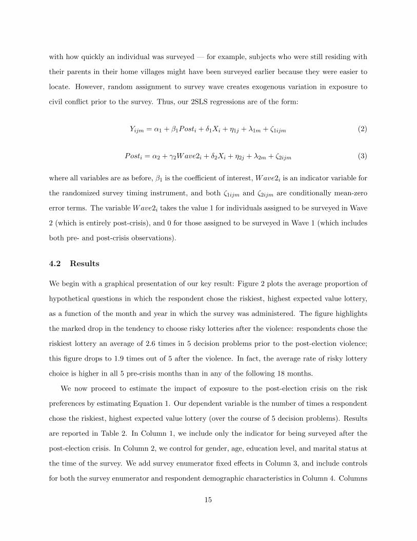
civil conflict prior to the survey. Thus, our 2SLS regressions are of the form:

Yijm = α1 + β1Posti + δ1Xi + η1j + λ1m + ζ1ijm (2)

Posti = α2 + γ2Wave2i + δ2Xi + η2j + λ2m + ζ2ijm (3)

where all variables are as before, β1 is the coefficient of interest, Wave2i is an indicator variable for

the randomized survey timing instrument, and both ζ1ijm and ζ2ijm are conditionally mean-zero

error terms. The variable Wave2i takes the value 1 for individuals assigned to be surveyed in Wave

2 (which is entirely post-crisis), and 0 for those assigned to be surveyed in Wave 1 (which includes

both pre- and post-crisis observations).

4.2 Results

We begin with a graphical presentation of our key result: Figure 2 plots the average proportion of

hypothetical questions in which the respondent chose the riskiest, highest expected value lottery,

as a function of the month and year in which the survey was administered. The figure highlights

the marked drop in the tendency to choose risky lotteries after the violence: respondents chose the

riskiest lottery an average of 2.6 times in 5 decision problems prior to the post-election violence;

this figure drops to 1.9 times out of 5 after the violence. In fact, the average rate of risky lottery

choice is higher in all 5 pre-crisis months than in any of the following 18 months.

We now proceed to estimate the impact of exposure to the post-election crisis on the risk

preferences by estimating Equation 1. Our dependent variable is the number of times a respondent

chose the riskiest, highest expected value lottery (over the course of 5 decision problems). Results

are reported in Table 2. In Column 1, we include only the indicator for being surveyed after the

post-election crisis. In Column 2, we control for gender, age, education level, and marital status at

the time of the survey. We add survey enumerator fixed effects in Column 3, and include controls

for both the survey enumerator and respondent demographic characteristics in Column 4. Columns

15

5 through 8 replicate 1 through 4 but include fixed effects for the month of the year in which the

survey took place.

In all eight OLS specifications reported in Table 2, the post-election coefficient is negative and

significant at at least the 99 percent confidence level, suggesting that experiencing the crisis lowered

the number of risky choices a respondent made by between 0.561 and 0.798 choices. In the pre-crisis

period, the average number of risky choices was only 2.566 out of five, so the change observed after

the crisis represents a dramatic drop in the willingness to bear profitable risk. Adding controls for

gender, education level, age, and marital status has almost no impact on the estimated coefficient.

In Table 3, we estimate analogous ordered logit specifications which account for the discrete but

ordered nature of the outcome, the number of risky choices. Again we find that the indicator for

being surveyed after the post-election violence is negative and significant (at at least the 99 percent

confidence level) in all specifications. In Table 4, we take an alternative approach to controlling for

time effects by including separate linear time trends in the pre- and post- crisis period. Columns

1 through 4 report OLS specifications, and Columns 5 through 8 report ordered logit results.

Again, the indicator for being surveyed in the post-crisis period is negative and significant in all

specifications.

As an additional set of robustness checks, we consider alternative formulations of the outcome

variable in Table 5. In the first column, the outcome variable is an indicator for always choosing the

highest variance and/or highest expected value lottery option (i.e. behaving in a manner consistent

with risk neutral or risk-loving preferences); in the second column, the outcome is an indicator for

always choosing the lowest variance alternative (i.e. behaving in a manner consistent with extreme

risk aversion). We find that the post-election violence led to a 5.7 percentage point (26 percent)

decrease in the likelihood of making risk neutral or risk loving choices, and an 11 percentage point

(82 percent) increase in the probability of always choosing the lowest variance (and lowest expected

return) lottery option. Next, we consider each decision problem in isolation. Importantly, this

allows us to test whether the effect that we find is likely to be driven by a change in the preference

for certainty, a finding that would be consistent with the results reported in Callen, Isaqzadeh,

Long, and Sprenger (2014).17 We find that the post-election violence led to a significant decrease

17Callen, Isaqzadeh, Long, and Sprenger (2014) find that Afghan respondents primed to recollect fearful episodes

16

in the likelihood of choosing the highest variance, highest expected value lottery option in each of

the five decision problems. Moreover, the effect is similar in magnitude across the four decision

problems that include three lottery alternatives; the estimated effect of violence does not appear

to be larger in decision problems that include a degenerate (i.e. risk-free) lottery as one of the

alternatives. We interpret this as evidence that the impact of violence does not only operate

through an increased preference for certainty.18 Thus, our main result is robust to a wide range of

alternative specifications.

Next, we employ a complementary identification strategy, exploiting the fact that KLPS2 re-

spondents were randomly assigned to one of two waves of surveying to generate instrumental

variables (IV) estimates of the impact of the post-election violence on measured risk aversion.19

IV regression results are reported in Table 6. In Column 1, we include only controls for gender,

age, education level, and marital status. Coefficient estimates indicate that the post-election crisis

had a large and statistically significant impact on measured risk preferences, reducing the num-

ber of times (out of five) that respondents opted for the riskiest, highest expected value lottery

by approximately one full question. Again, relative to a mean number of risky choices of about

2.5 in the pre-crisis period, this is an extremely large effect. In Columns 2 through 4 we include

additional controls for the identity of the survey enumerator and the month in which the interview

took place. Coefficient estimates are consistently negative and significant. Thus, our IV estimates

are consistent with our un-instrumented results: Kenya’s post-election crisis appears to have made

survey respondents substantially more risk averse.

display greater risk aversion when certainty is an option, but greater risk tolerance when no risk-free alternativesare available. They interpret this as evidence that subjects display a preference for certainty not consistent withexpected utility maximization; their evidence suggests that violence impacts this preference for certainty.

18To further probe this issue, we examine the likelihood of choosing the safest (i.e. lowest variance, lowest return)lottery alternative in each of the five decision problems. Results are reported in the Online Appendix. We findno evidence that the shift away from high-risk lotteries is stronger in decision problems that included options withpurely certain outcomes.

19Before proceeding to our IV analysis, we check whether the random assignment of respondents to survey wavesgenerated groups that were comparable in terms of observable characteristics at the start of the survey. We focus onfixed traits and outcomes that were recorded in the survey for specific points in time. For example, the survey collectsdetailed information about school participation in each year between 1998 and the moment of the interview; thisallows us to generate a variable indicating the number of years of schooling that a respondent had completed at thestart of 2007, regardless of the year in which a respondent was actually surveyed. Results are reported in the OnlineAppendix. We find no statistically significant differences between the survey waves in terms of proportion female,age in 2007, proportion from the local-majority Luhya ethnic group, years of schooling completed by 2007, and theproportion that were married by 2007. Thus, the randomization appears to have succeeded in creating groups ofrespondents that are similar in terms of observable characteristics.

17

4.3 Potential Mechanisms

We interpret our results as evidence that civil conflict impacts individual risk preferences. One

alternative explanation is that the post-election violence was an economic shock, and that young

adults expected it to slow growth and reduce job opportunities; if those with higher expected

permanent incomes are more willing to bear risk, such a shock might have impacted risk preferences

through job prospects. In the Online Appendix, we show that the post-election crisis did not have

a significant impact on the likelihood of being engaged in any off-farm income-generating activity.

In fact, there is some evidence that the post-election violence led to an increase in the likelihood of

working for a wage, though the effect is not significant in the IV specification. As expected given

the estimated impact on risk preferences, we find that self-employment is significantly less common

after the violence — highlighting a potential channel through which conflict may slow growth and

development.

Voors, Nillesen, Verwimp, Bulte, Lensink, and Van Soest (2012) suggest another potential

mechanism through which conflict might change preferences and behavior: the social context may

change in the wake of violence. We find some evidence consistent with this hypothesis: after the

violence, KLPS2 respondents displayed significantly less generalized trust (as measured through

their responses to the standard question: “Generally speaking, do you think that most people can

be trusted, or would they try to take advantage of you if they got the chance?”).20 Violence may

impact many aspects of society, and it is impossible to fully distinguish between mechanisms and

other outcomes. Moreover, as other have noted, the willingness to trust and the willingness to take

risks are, from a theoretical perspective, closely related (Karlan 2005, Schechter 2007). However,

the evidence suggests that the post-election violence did not impact risk preferences purely through

a labor market channel; instead, we find suggestive evidence that the violence changed the social

context by altering both preferences and beliefs about others.

20Results reported in the Online Appendix.

18

5 Conclusion

We measure the impact of Kenya’s post-election violence on individual risk preferences. We find

that experiencing the post-election crisis appears to have increased measured risk aversion signifi-

cantly. Point estimates suggest that exposure to the crisis decreased the likelihood of making risk

neutral or risk loving choices by 5.7 percentage points (26 percent), and increase the likelihood

of always choosing the lowest variance, lowest expected value lottery by 11 percentage points (82

percent). Our results are robust to a range of controls and the use of entirely distinct identification

strategies. Thus, the evidence suggests that exposure to the post-election crisis led to a statistically

and economically significant decrease in the willingness to take profitable risks.

In relation to existing studies of the determinants of individual preferences, our results cor-

roborate a growing body of evidence that preferences are impacted by major life events such as

conflict, disasters, and economic downturns. Identification of the impacts of such major events is

always challenging since exogenous variation in exposure to historical shocks is rare. This paper

may be unique in the timing of data collection in relation to the event in question: we are aware

of no other study of risk preferences with data collection ongoing in the immediate run-up to and

aftermath of a major event of this kind.

Existing studies of the impact of conflict on individual preferences estimate the marginal impact

of greater exposure to violence, implicitly treating less-exposed survivors as a comparison group. We

are able to expand this literature because our identification strategies enable us to measure the effect

of civil conflict on the general population. Relatively more conflict-affected individuals may become

more pro-social or less risk averse (Bellows and Miguel 2009, Blattman 2009, Voors, Nillesen,

Verwimp, Bulte, Lensink, and Van Soest 2012, Callen, Isaqzadeh, Long, and Sprenger 2014), but

the overall impact on the population as a whole is a shift toward less willingness to take profitable

risks. Moreover, our results suggest that the channel of impact is social and not (primarily)

economic, since the probability of engaging in any income-generating activity is not impacted by

the violence, but generalized trust in others is. Our results therefore suggest that conflict may have

long-lasting impacts on economic development through channels such as reduced entrepreneurship.

That our findings differ from some earlier studies suggests that the impacts of conflict at the scale

19

of affected individuals and villages may not generalize to the scale of a district, or that of a nation.

20

References

Agina, B. (2007): “Raila’s third win,” The Standard, Online: https://web.archive.org/web/

20071113172711/http://www.eastandard.net/news/?id=1143976568, Accessed on July 29,2015.

Andreoni, J., and C. Sprenger (2010): “Certain and Uncertain Utility: The Allais Paradoxand Five Decision Theory Phenomena,” working paper.

Ashraf, N., D. Karlan, and W. Yin (2006): “Tying Odysseus to the Mast: Evidence froma Commitment Savings Product in the Philippines,” Quarterly Journal of Economics, 121(2),635–672.

Baird, S., C. Blattman, L. Casaburi, D. K. Evans, J. Hamory, M. Kremer, E. Miguel,O. Ozier, S. Y. Siegel, P. Wafula, and E. Yeh (2007): “The Kenyan Life Panel Survey(KLPS) Round 1: Survey Data Users Guide,” Discussion paper.

Barr, A., and G. Genicot (2008): “Risk Pooling, Commitment and Information: An Experi-mental Test,” Journal of the European Economic Association, 6(6), 1151–1185.

Bauer, M., A. Cassar, J. Chytilova, and J. Henrich (2013): “War’s Enduring Effects onthe Development of Egalitarian Motivations and In-Group Biases,” Psychological Science, p.0956797613493444.

BBC (2008a): “Deal to end Kenyan crisis agreed,” BBC News, Online: http://news.bbc.co.uk/2/hi/africa/7344816.stm, Accessed on July 24, 2015.

(2008b): “Kenya rivals agree to share power,” BBC News, Online: http://news.bbc.

co.uk/2/hi/africa/7268903.stm, Accessed on July 28, 2015.

BBC News (2007): “Odinga rejects Kenya poll result,” BBC News, Online: http://news.bbc.

co.uk/2/hi/africa/7165406.stm, Accessed on July 29, 2015.

Bellows, J., and E. Miguel (2009): “War and Local Collective Action in Sierra Leone,” Journalof Public Economics, 93(11), 1144–1157.

Binswanger, H. P. (1980): “Attitudes toward Risk: Experimental Measurement in Rural India,”American Journal of Agricultural Economics, 62(3), 395–407.

Blattman, C. (2009): “From Violence to Voting: War and Political Participation in Uganda,”American Political Science Review, 103(02), 231–247.

Blattman, C., and J. Annan (2010): “The Consequences of Child Soldiering,” The Review ofEconomics and Statistics, 92(4), 882–898.

Blattman, C., and E. Miguel (2010): “Civil War,” Journal of Economic Literature, 48(1),3–57.

Bryan, G., S. Chowdhury, and A. M. Mobarak (2014): “Underinvestment in a ProfitableTechnology: The Case of Seasonal Migration in Bangladesh,” Econometrica, 82(5), 1671–1748.

21

Callen, M., M. Isaqzadeh, J. D. Long, and C. Sprenger (2014): “Violence and RiskPreference: Experimental Evidence from Afghanistan,” The American Economic Review, 104(1),123–148.

Camerer, C. (1995): “Individual Decision Making,” in The Handbook of Experimental Economics,ed. by J. Kagel, and A. Roth, pp. 587–673. Princeton University Press, Princeton.

Camerer, C. F., and R. M. Hogarth (1999): “The Effects of Financial Incentives in Experi-ments: A Review and Capital-Labor-Production Framework,” Journal of Risk and Uncertainty,19(1-3), 7–42.

Cameron, L., and M. Shah (2013): “Risk-Taking Behavior in the Wake of Natural Disasters,”NBER Working Paper 19534, National Bureau of Economic Research.

Choi, S., S. Kariv, W. Muller, and D. Silverman (2014): “Who Is (More) Rational?,”American Economic Review, 104(6), 1518–1550.

Collier, P., V. Elliott, H. Hegre, A. Hoeffler, M. Reynal-Querol, and N. Sambanis(2003): “Breaking the Conflict Trap: Civil War and Development Policy,” .

Eckel, C. C., M. A. El-Gamal, and R. K. Wilson (2009): “Risk Loving After the Storm:A Bayesian-Network Study of Hurricane Katrina Evacuees,” Journal of Economic Behavior &Organization, 69(2), 110–124.

Eckel, C. C., and P. J. Grossman (2008): “Forecasting risk attitudes: An experimental studyusing actual and forecast gamble choices,” Journal of Economic Behavior and Organization,68(1), 1–17.

Fisman, R., P. Jakiela, and S. Kariv (2014): “The Distributional Preferences of Americans,”NBER working paper no. 20145.

(2015): “How Did Distributional Preferences Change During the Great Recession?,”Journal of Public Economics, 128, 84–95.

Fisman, R., P. Jakiela, S. Kariv, and D. Markovits (2015): “The Distributional Preferencesof an Elite,” Science, 349(6254), 1300.

Hanaoka, C., H. Shigeoka, and Y. Watanabe (2015): “Do Risk Preferences Change? Evi-dence from Panel Data Before and After the Great East Japan Earthquake,” NBER WorkingPaper 21400, National Bureau of Economic Research.

Hey, J. D., and C. Orme (1994): “Investigating Generalizations of Expected Utility TheoryUsing Experimental Data,” Econometrica, 62(6), 1291–1326.

Hjort, J. (forthcoming): “Ethnic Divisions and Production in Firms,” Quarterly Journal ofEconomics.

Holt, C. A., and S. K. Laury (2002): “Risk Aversion and Incentive Effects,” American Eco-nomic Review, 92(5), 1644–1655.

Humphreys, M., and J. M. Weinstein (2006): “Handling and Manhandling Civilians in CivilWar,” American Political Science Review, 100(3), 429–447.

22

Jaeger, D. A., T. Dohmen, A. Falk, D. Huffman, U. Sunde, and H. Bonin (2010):“Direct Evidence on Risk Attitudes and Migration,” The Review of Economics and Statistics,92(3), 684–689.

Jakiela, P., and O. Ozier (forthcoming): “Does Africa Need a Rotten Kin Theorem? Experi-mental Evidence from Village Economies,” The Review of Economic Studies.

Jing, L. (2015): “Plastic Surgery or Primary Care? Altruistic Preferences and Expected SpecialtyChoice of U.S. Medical Students,” working paper.

Kahneman, D., and A. Tversky (1979): “Prospect theory: An analysis of decision under risk,”Econometrics, 47(2), 263–291.

Karlan, D. S. (2005): “Using Experimental Economics to Measure Social Capital and PredictFinancial Decisions,” American Economic Review, 95(5), 1688–1699.

Kosegi, B., and M. Rabin (2006): “A Model of Reference-Dependent Preferences,” QuarterlyJournal of Economics, 121(4), 1133–1166.

Levitt, S. D., and J. A. List (2007): “What Do Laboratory Experiments Measuring SocialPreferences Tell Us About the Real World?,” Journal of Economic Perspectives, 21(2), 153–174.

Liu, E. M. (2013): “Time to Change What to Sow: Risk Preferences and Technology AdoptionDecisions of Cotton Farmers in China,” Review of Economics and Statistics, 95(4), 1386–1403.

Liu, E. M., and J. Huang (2013): “Risk Preferences and Pesticide Use by Cotton Farmers inChina,” Journal of Development Economics, 103, 202–215.

Loomes, G. (2005): “Modelling the Stochastic Component of Behaviour in Experiments: SomeIssues for the Interpretation of Data,” Experimental Economics, 8(4), 301–323.

Malmendier, U., and S. Nagel (2011): “Depression Babies: Do Macroeconomic ExperiencesAffect Risk-Taking?,” Quarterly Journal of Economics, 126(1), 373–416.

McCrummen, S. (2007): “Incumbent declared winner in Kenya’s disputed election,” Washing-ton Post, Online: http://www.washingtonpost.com/wp-dyn/content/article/2007/12/30/

AR2007123002506_pf.html, Accessed on July 24, 2015.

Meier, S., and C. Sprenger (2012): “Time Discounting Predicts Creditworthiness,” Psycholog-ical Science, 23(1), 56–58.

Miguel, E., and M. Kremer (2004): “Worms: Identifying Impacts on Education and Health inthe Presence of Treatment Externalities,” Econometrica, 72(1), 159–217.

Miguel, E., and G. Roland (2011): “The Long-Run Impact of Bombing Vietnam,” Journal ofDevelopment Economics, 96(1), 1–15.

Munene, M., and J. Otieno (2007): “Kenya: Raila Tops Table,” Daily Nation, Online: http://allafrica.com/stories/200709281185.html, Accessed on July 29, 2015.

Nunn, N., and L. Wantchekon (2011): “The Slave Trade and the Origins of Mistrust in Africa,”The American Economic Review, 101(7), 3221–3252.

23

Otieno, J. (2007): “New Poll Predicts Close Race,” Daily Nation, Online: https:

//web.archive.org/web/20080212172025/http://politics.nationmedia.com/inner.

asp?pcat=NEWS&cat=TOP&sid=908, Accessed on July 29, 2015.

Pettersson, T., and P. Wallensteen (2015): “Armed Conflicts, 1946–2014,” Journal of PeaceResearch, 52(4), 536–550.

Schechter, L. (2007): “Traditional Trust Measurement and the Risk Confound: An Experimentin Rural Paraguay,” Journal of Economic Behavior and Organization, 62(2), 272–292.

Schumpeter, J. A. (1934): The Theory of Economic Development: An Inquiry into Profits,Capital, Credit, Interest, and the Business Cycle, vol. 55. Transaction Publishers.

(1939): Business Cycles, vol. 1. Cambridge University Press.

Skriabikova, O. J., T. Dohmen, and B. Kriechel (2014): “New Evidence on the Relationshipbetween Risk Attitudes and Self-Employment,” Labour Economics, 30, 176–184.

Standard Team (2007): “Last Poll, Last Push,” The Standard, Online: https://web.archive.org/web/20071220153404/http://www.eastandard.net/news/?id=1143979128, Accessed onJuly 29, 2015.

Stigler, G. J., and G. S. Becker (1977): “De Gustibus Non Est Disputandum,” AmericanEconomic Review, 67(2), 76–90.

Tanaka, T., C. F. Camerer, and Q. Nguyen (2010): “Risk and Time Preferences: LinkingExperimental and Household Survey Data from Vietnam,” American Economic Review, 100(1),557–571.

Van Praag, N. (2010): “View from the bottom: the conspiracy of violence in Nairobi’s slums,”World Bank Conflict and Development Blog, Online: http://blogs.worldbank.org/conflict/slums-in-mathare-kenya, Accessed on July 24, 2015.

Von Gaudecker, H.-M., A. van Soest, and E. Wengstrom (2011): “Heterogeneity in RiskyChoice Behavior in a Broad Population,” American Economic Review, 101(2), 664–694.

Voors, M., T. Turley, A. Kontoleon, E. Bulte, and J. A. List (2012): “Exploring whetherBehavior in Context-Free Experiments is Predictive of Behavior in the Field: Evidence from Laband Field Experiments in Rural Sierra Leone,” Economics Letters, 114(3), 308–311.

Voors, M. J., E. E. Nillesen, P. Verwimp, E. H. Bulte, R. Lensink, and D. P. Van Soest(2012): “Violent Conflict and Behavior: a Field Experiment in Burundi,” The American Eco-nomic Review, 102(2), 941–964.

Waki, P. N. (2008): Report of the Commission of Inquiry into Post Election Violence (CIPEV).Government Printer.

World Bank (2006): “Kenya Governance Draft Report/Note,” Report 38196, The World Bank.

(2008): “Cities of Hope? Governance, economic and human challenges of Kenya’s fivelargest cities,” Report 46988, World Bank Water and Urban Unit 1, Africa Region.

24

(2009): “Kenya Economic Development, Police Oversight, and Accountability,” Report44515-KE, The World Bank Public Sector Reform and Capacity Building Unit, Africa Region.

(2010a): “Country Partnership Strategy for the Republic of Kenya for the period FY2010-13,” Report 52521-KE, The International Development Association, The International FinanceCorporation, and the Multilateral Investment Guarantee Agency.

(2010b): “Public Sentinel: News Media and Governance Reform,” Report 51842, TheWorld Bank.

(2011): “Kenya Economic Update Edition 5: Navigating the storm, Delivering thepromise,” Report 66308, World Bank Poverty Reduction and Economic Management Unit, AfricaRegion.

(2012): “Kenya Economic Update Edition 7: Kenya at work,” Report 7, World BankKenya Country Office.

25

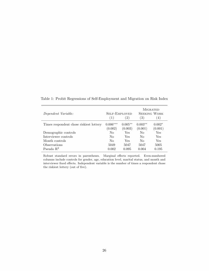
Table 1: Probit Regressions of Self-Employment and Migration on Risk Index

MigratedDependent Variable: Self-Employed Seeking Work

(1) (2) (3) (4)

Times respondent chose riskiest lottery 0.006∗∗∗ 0.005∗∗ 0.003∗∗ 0.002∗

(0.002) (0.003) (0.001) (0.001)Demographic controls No Yes No YesInterviewer controls No Yes No YesMonth controls No Yes No YesObservations 5049 5047 5047 5005Pseudo R2 0.002 0.095 0.004 0.195

Robust standard errors in parentheses. Marginal effects reported. Even-numberedcolumns include controls for gender, age, education level, marital status, and month andinterviewer fixed effects. Independent variable is the number of times a respondent chosethe riskiest lottery (out of five).

26

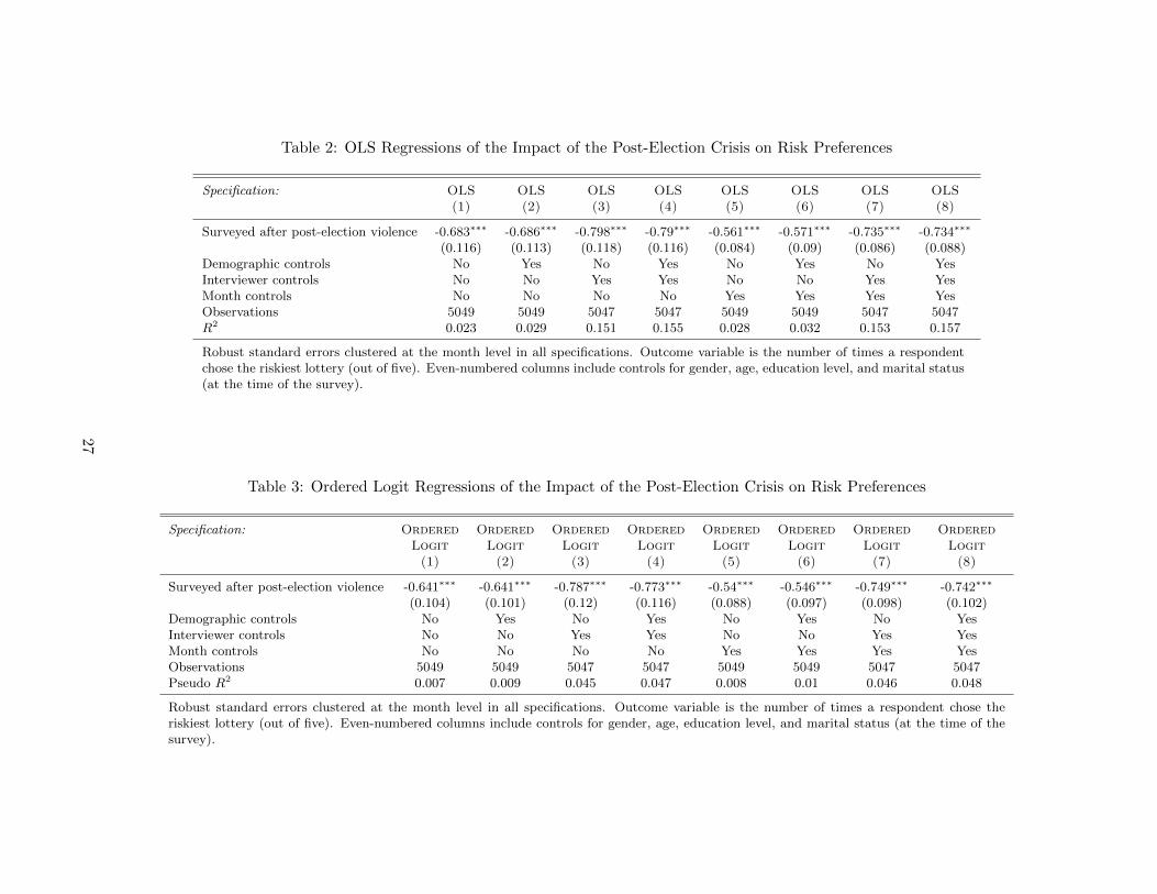
Table 2: OLS Regressions of the Impact of the Post-Election Crisis on Risk Preferences

Specification: OLS OLS OLS OLS OLS OLS OLS OLS(1) (2) (3) (4) (5) (6) (7) (8)

Surveyed after post-election violence -0.683∗∗∗ -0.686∗∗∗ -0.798∗∗∗ -0.79∗∗∗ -0.561∗∗∗ -0.571∗∗∗ -0.735∗∗∗ -0.734∗∗∗

(0.116) (0.113) (0.118) (0.116) (0.084) (0.09) (0.086) (0.088)Demographic controls No Yes No Yes No Yes No YesInterviewer controls No No Yes Yes No No Yes YesMonth controls No No No No Yes Yes Yes YesObservations 5049 5049 5047 5047 5049 5049 5047 5047R2 0.023 0.029 0.151 0.155 0.028 0.032 0.153 0.157

Robust standard errors clustered at the month level in all specifications. Outcome variable is the number of times a respondentchose the riskiest lottery (out of five). Even-numbered columns include controls for gender, age, education level, and marital status(at the time of the survey).

Table 3: Ordered Logit Regressions of the Impact of the Post-Election Crisis on Risk Preferences

Specification: Ordered Ordered Ordered Ordered Ordered Ordered Ordered OrderedLogit Logit Logit Logit Logit Logit Logit Logit(1) (2) (3) (4) (5) (6) (7) (8)

Surveyed after post-election violence -0.641∗∗∗ -0.641∗∗∗ -0.787∗∗∗ -0.773∗∗∗ -0.54∗∗∗ -0.546∗∗∗ -0.749∗∗∗ -0.742∗∗∗

(0.104) (0.101) (0.12) (0.116) (0.088) (0.097) (0.098) (0.102)Demographic controls No Yes No Yes No Yes No YesInterviewer controls No No Yes Yes No No Yes YesMonth controls No No No No Yes Yes Yes YesObservations 5049 5049 5047 5047 5049 5049 5047 5047Pseudo R2 0.007 0.009 0.045 0.047 0.008 0.01 0.046 0.048

Robust standard errors clustered at the month level in all specifications. Outcome variable is the number of times a respondent chose theriskiest lottery (out of five). Even-numbered columns include controls for gender, age, education level, and marital status (at the time of thesurvey).

27

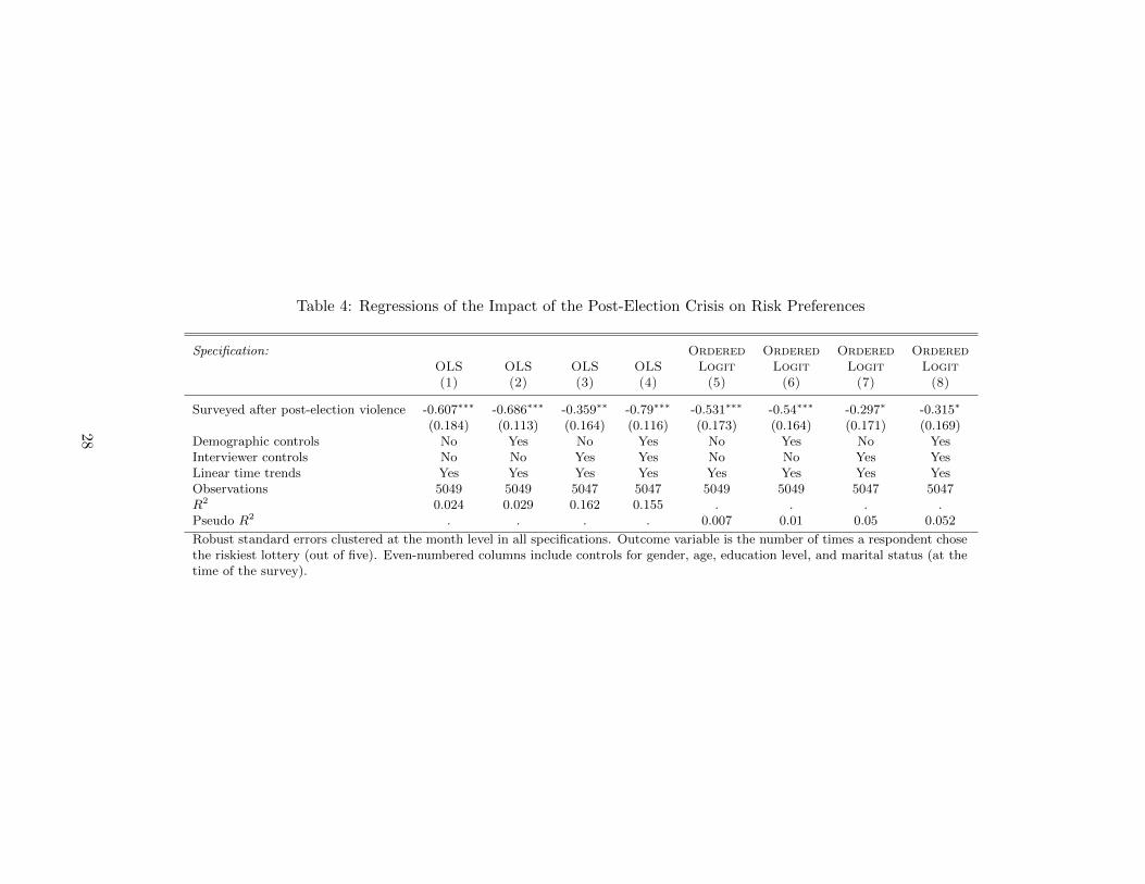
Table 4: Regressions of the Impact of the Post-Election Crisis on Risk Preferences

Specification: Ordered Ordered Ordered OrderedOLS OLS OLS OLS Logit Logit Logit Logit(1) (2) (3) (4) (5) (6) (7) (8)

Surveyed after post-election violence -0.607∗∗∗ -0.686∗∗∗ -0.359∗∗ -0.79∗∗∗ -0.531∗∗∗ -0.54∗∗∗ -0.297∗ -0.315∗

(0.184) (0.113) (0.164) (0.116) (0.173) (0.164) (0.171) (0.169)Demographic controls No Yes No Yes No Yes No YesInterviewer controls No No Yes Yes No No Yes YesLinear time trends Yes Yes Yes Yes Yes Yes Yes YesObservations 5049 5049 5047 5047 5049 5049 5047 5047R2 0.024 0.029 0.162 0.155 . . . .Pseudo R2 . . . . 0.007 0.01 0.05 0.052

Robust standard errors clustered at the month level in all specifications. Outcome variable is the number of times a respondent chosethe riskiest lottery (out of five). Even-numbered columns include controls for gender, age, education level, and marital status (at thetime of the survey).

28

Table 5: Robustness Checks: OLS Regressions of the Impact of the Post Election Violence on Alternate Measures of Risk Aversion

Dependent Variable: Risk neutral Most — Choice on decision number. . . —or loving risk averse 2 3 4 5 6

(1) (2) (3) (4) (5) (6) (7)

Surveyed after post-election violence -0.057∗∗∗ 0.11∗∗∗ -0.114∗∗∗ -0.234∗∗∗ -0.296∗∗∗ -0.29∗∗∗ -0.26∗∗∗

(0.017) (0.023) (0.027) (0.045) (0.06) (0.03) (0.053)Observations 5049 5049 5049 5049 5049 5049 5049R2 0.007 0.033 0.015 0.017 0.027 0.023 0.025

Robust standard errors clustered at the month level in all specifications. All specifications include controls for gender, age,education level, and marital status (at the time of the survey). Thus, the specifications in this table mirror those in Table 2,Column 2. Here, the outcome variables vary by column. The outcome in Column 1 is an indicator for making risk neutral or riskloving choices. Column 2 is an indicator for making the most risk averse choice on every card, so its sign is opposite those in othercolumns and tables. Columns 3 through 7 use discrete representations of the separate decision cards as outcomes, ordered by riskaversion; thus, the first two of these are indicator variables for taking the riskier option, while the remaining three are variablesthat take on the values 1, 2, and 3, with 1 being least risky, and 3 being riskiest.

29

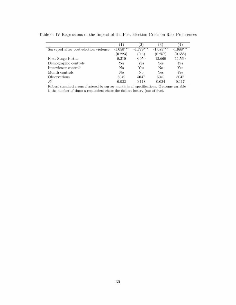
Table 6: IV Regressions of the Impact of the Post-Election Crisis on Risk Preferences

(1) (2) (3) (4)Surveyed after post-election violence -1.050∗∗∗ -1.779∗∗∗ -1.085∗∗∗ -1.988∗∗∗

(0.223) (0.5) (0.257) (0.588)First Stage F-stat 9.210 8.050 13.660 11.560Demographic controls Yes Yes Yes YesInterviewer controls No Yes No YesMonth controls No No Yes YesObservations 5049 5047 5049 5047R2 0.022 0.118 0.024 0.117Robust standard errors clustered by survey month in all specifications. Outcome variableis the number of times a respondent chose the riskiest lottery (out of five).

30

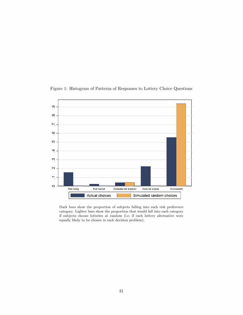
Figure 1: Histogram of Patterns of Responses to Lottery Choice Questions

Dark bars show the proportion of subjects falling into each risk preferencecategory. Lighter bars show the proportion that would fall into each categoryif subjects choose lotteries at random (i.e. if each lottery alternative wereequally likely to be chosen in each decision problem).

31

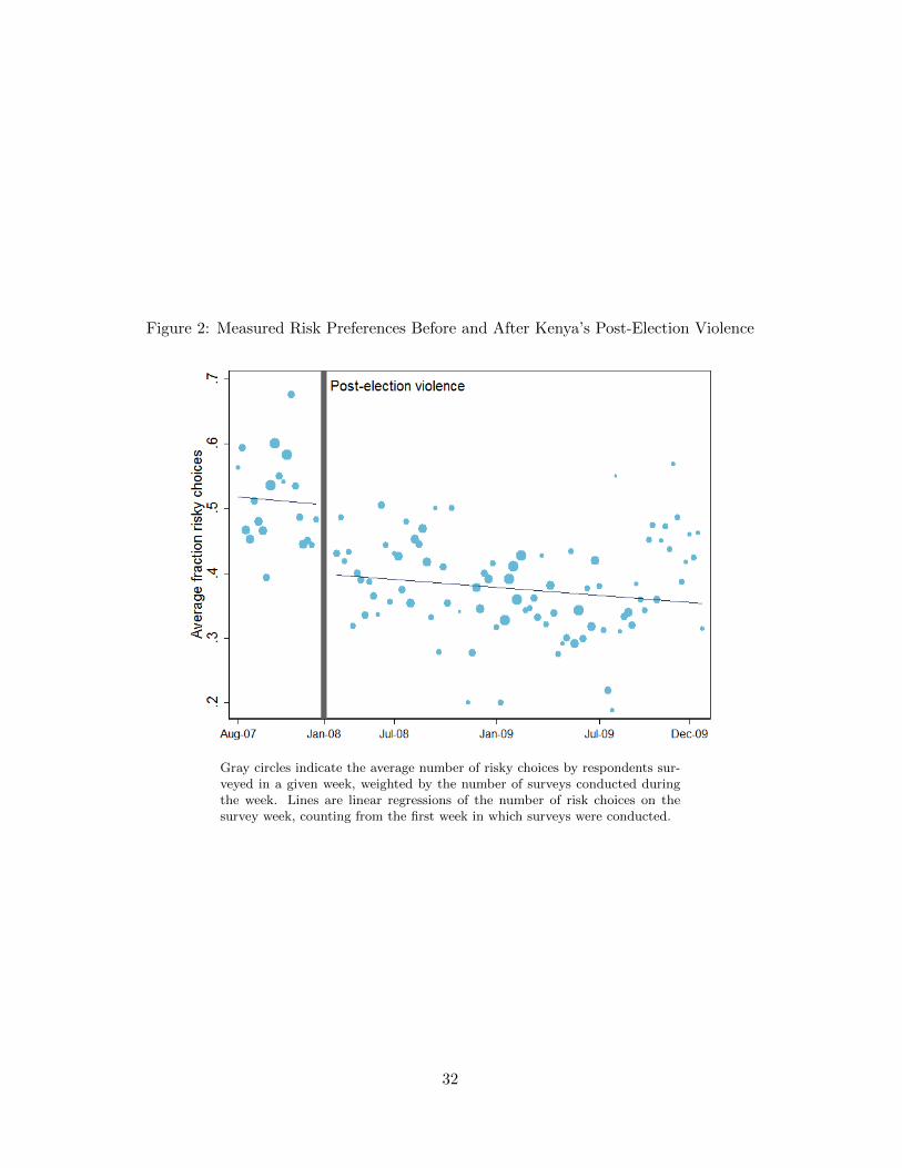
Figure 2: Measured Risk Preferences Before and After Kenya’s Post-Election Violence

Gray circles indicate the average number of risky choices by respondents sur-veyed in a given week, weighted by the number of surveys conducted duringthe week. Lines are linear regressions of the number of risk choices on thesurvey week, counting from the first week in which surveys were conducted.

32

A Online Appendix: not for print publication

Table A1: Decision Problems Embedded in Kenyan Life Panel Survey 2

Option A Option B Option CHeads Tails Heads Tails Heads Tails

Practice Decision Problem 1 100 100 150 150 - -Practice Decision Problem 2 100 150 200 250 - -

Decision Problem 1 100 100 100 120 - -Decision Problem 2 100 100 0 400 - -Decision Problem 3 30 340 100 100 0 400Decision Problem 4 100 100 55 240 30 340Decision Problem 5 30 230 60 170 90 110Decision Problem 6 10 200 70 160 90 110

All payouts in Kenyan shillings.

Table A2: Balance Check: KLPS2 Wave1 vs. Wave 2 Comparison

Variable Wave 1 Wave 2 Difference

Number of observations 2469 2580Female 0.49 0.49 0.00

(0.01) (0.01) (0.01)Age in 2007 21.13 21.21 0.09

(0.05) (0.05) (0.07)Highest grade completed by 2006 8.56 8.48 -0.08

(0.04) (0.04) (0.06)Married by 2006 0.31 0.30 -0.01

(0.01) (0.01) (0.01)

Standard errors in parentheses.

A1

Table A3: Potential Mechanisms: Impacts on Labor Market Outcomes and Generalized Trust

Non-farm Wage Self- Trustwork work employment others(1) (2) (3) (4)

Panel A: OLS

Surveyed after post-election violence 0.027 0.059∗∗∗ -0.035∗∗ -0.057∗∗∗

(0.029) (0.018) (0.016) (0.011)Observations 5049 5047 5049 5047R2 0.134 0.088 0.064 0.016

Panel B: IV

Surveyed after post-election violence -0.043 0.029 -0.071∗∗ -0.095∗∗∗

(0.06) (0.053) (0.033) (0.024)First Stage F-stat 9.210 9.210 9.210 9.210Observations 5049 5047 5049 5047R2 0.118 0.086 0.047 0.012

Robust standard errors clustered by survey month in all specifications. Panel A follows thespecification in Table 2, Column 2. Panel B follows the specification in Table 6, Column 2.The outcomes in Columns 1 through 3 are indicator variables: the second and third columnsare indicators for the respondent currently having wage work or self-employment; and the firstcolumn is an indicator for having either of these. In Column 4, the outcome is also binary,but is a representation of respondents’ answer to the World Values Survey question:“Generallyspeaking, do you think that most people can be trusted or that you need to be very careful indealing with people?”

Table A4: Robustness Checks: Impact of the Post Election Violence on Choosing Safest Alternative

Dependent Variable: — Safest Choice on decision number. . . —2 3 4 5 6(1) (2) (3) (4) (5)

Surveyed after post-election violence 0.114∗∗∗ 0.114∗∗∗ 0.11∗∗∗ 0.204∗∗∗ 0.18∗∗∗

(0.027) (0.027) (0.029) (0.015) (0.027)Observations 5049 5049 5049 5049 5049R2 0.015 0.017 0.019 0.037 0.033

Robust standard errors clustered at the month level in all specifications. All specificationsinclude controls for gender, age, education level, and marital status (at the time of thesurvey). Thus, the specifications in this table mirror those in Table 2, Column 2. Theoutcome in each case is an indicator variable for taking the safest option in a given decision.

A2

Figure A1: Histograms of Individual Choices in Each Decision Problem

Decision Problem 1 Decision Problem 2

Decision Problem 3 Decision Problem 4

Decision Problem 5 Decision Problem 6

A3