
Simulation of efficiency and time resolution of Resistive Plate Chambers at high rate

UNIVERSITÀ DEL SALENTO
DIPARTIMENTO DI FISICA
DOTTORATO DI RICERCA IN FISICA – XXII CICLO
Off-line monitoring and data quality ofResistive Plate Chambers for the ATLAS
experiment
Supervisors: Candidate:
Prof. Edoardo Gorini Angelo Guida
Dr. Gabriele Chiodini
Thesis submitted for the degree of Doctor of Philosophy

Io stimo più il trovar un vero,benché di cosa leggiera,
che ’l disputar lungamente delle massime questionisenza conseguir verità nissuna.
G. Galilei

Contents
Introduction 1
1 The standard model of elementary particles 51.1 The Standard Model. . . . . . . . . . . . . . . . . . . . . . . . 5
1.1.1 Particles and fundamental interactions. . . . . . . . . . . 51.2 The Electro-weak theory. . . . . . . . . . . . . . . . . . . . . . 7
1.2.1 The spontaneous symmetry breaking mechanism. . . . . 81.3 Higgs boson mass constraints. . . . . . . . . . . . . . . . . . . . 12
1.3.1 Theoretical limits. . . . . . . . . . . . . . . . . . . . . . 121.3.2 Experimental limits. . . . . . . . . . . . . . . . . . . . . 12
1.4 Supersymmetry. . . . . . . . . . . . . . . . . . . . . . . . . . . 151.4.1 Open questions in standard model. . . . . . . . . . . . . 151.4.2 Supersymmetry. . . . . . . . . . . . . . . . . . . . . . . 16
1.5 Higgs search at LHC. . . . . . . . . . . . . . . . . . . . . . . . 171.5.1 Standard Model Higgs. . . . . . . . . . . . . . . . . . . 171.5.2 Supersymmetric Higgs. . . . . . . . . . . . . . . . . . . 20
2 The ATLAS experiment at Large Hadron Collider 232.1 The Large Hadron Collider. . . . . . . . . . . . . . . . . . . . . 232.2 The ATLAS experiment at LHC. . . . . . . . . . . . . . . . . . 27
2.2.1 Magnet system. . . . . . . . . . . . . . . . . . . . . . . 272.2.2 Inner detector. . . . . . . . . . . . . . . . . . . . . . . . 282.2.3 The calorimeter system. . . . . . . . . . . . . . . . . . . 302.2.4 The ATLAS Muon Spectrometer. . . . . . . . . . . . . . 302.2.5 Trigger Chambers. . . . . . . . . . . . . . . . . . . . . 402.2.6 Trigger and data acquisition system. . . . . . . . . . . . 42
3 ATLAS RPC trigger chambers 453.1 Resistive Plate Chambers. . . . . . . . . . . . . . . . . . . . . . 453.2 The ATLAS RPC . . . . . . . . . . . . . . . . . . . . . . . . . . 46
3.2.1 Readout panels and front-end electronics. . . . . . . . . 473.3 ATLAS RPC detector layout. . . . . . . . . . . . . . . . . . . . 503.4 ATLAS Barrel Muon Trigger. . . . . . . . . . . . . . . . . . . . 50
3.4.1 Trigger hardware implementation. . . . . . . . . . . . . 52
iii

iv CONTENTS
4 RPC Offline Monitoring 574.1 ATLAS software infrastructure. . . . . . . . . . . . . . . . . . . 57
4.1.1 The Athena framework. . . . . . . . . . . . . . . . . . . 574.1.2 Data reconstruction process. . . . . . . . . . . . . . . . 59
4.2 RPC off-line monitoring . . . . . . . . . . . . . . . . . . . . . . 604.3 Detector and readout electronics monitoring. . . . . . . . . . . . 63
4.3.1 Readout electronics plots. . . . . . . . . . . . . . . . . . 664.3.2 Detector plots. . . . . . . . . . . . . . . . . . . . . . . . 71
4.4 RPC and MDT correlation monitoring. . . . . . . . . . . . . . . 784.5 RPC track monitoring. . . . . . . . . . . . . . . . . . . . . . . . 79
5 RPC Data Quality 875.1 Muon Spectrometer Data Quality Chain. . . . . . . . . . . . . . 875.2 RPC Data Quality. . . . . . . . . . . . . . . . . . . . . . . . . . 89
5.2.1 RPC Shifter plots. . . . . . . . . . . . . . . . . . . . . . 895.2.2 Data Quality Monitoring Framework. . . . . . . . . . . 955.2.3 RPC Data Quality plots. . . . . . . . . . . . . . . . . . . 97
5.3 Summary plots . . . . . . . . . . . . . . . . . . . . . . . . . . . 101
6 Performance of ATLAS RPC detector 1076.1 Introduction. . . . . . . . . . . . . . . . . . . . . . . . . . . . . 1076.2 Studies with cosmics data. . . . . . . . . . . . . . . . . . . . . . 107
6.2.1 RPC coverage. . . . . . . . . . . . . . . . . . . . . . . . 1096.2.2 RPC efficiency. . . . . . . . . . . . . . . . . . . . . . . 1096.2.3 Performance from off-line monitoring. . . . . . . . . . . 1176.2.4 RPC Efficiency and Cluster Size as a function of high
voltage . . . . . . . . . . . . . . . . . . . . . . . . . . . 1206.3 Studies with beam data. . . . . . . . . . . . . . . . . . . . . . . 124
6.3.1 Beam collimator scraping events. . . . . . . . . . . . . . 1246.3.2 Beams collisions. . . . . . . . . . . . . . . . . . . . . . 127
6.4 Conclusions. . . . . . . . . . . . . . . . . . . . . . . . . . . . . 129
Summary and Outlook 131
Bibliography 132

Introduction
This thesis describes the developed software, the experimental techniques and theanalysis results for monitoring and assessing data qualityof ATLAS RPC triggerchambers.
ATLAS is an experiment currently running at the Large HadronCollider (LHC)at CERN laboratory, in Geneva. LHC is the most energetic accelerator in theworld. Its main features are three:Luminosity, andEnergy. The LHC acceleratoris designed to provide proton-proton collisions at the center of mass energy of 14TeV at a luminosity of1034cm−2s−1 with a bunch crossing rate of25ns. At thetime of writing it is providing collision at half of design energy but almost a factorof four higher than achieved in previous accelerators.
The main physics goal of the ATLAS experiment is the discovery of the Higgsboson. In the theoretical frame of the Standard Model the Higgs boson is respon-sible of the observed mass of elementary particles. In addition, ATLAS has a largecapability to discovernew physics, as for examplesuper-symmetricparticles, ex-ploring the TeV energy scale range.
One of the two major experiments installed at the LHC is the ATLAS detector.It is a general purpose experiment designed to cover the fullrange of the physicalprocesses that will be produced by LHC collisions. It is composed of several sub-detectors with very well defined purpose: a central trackingsystem to reconstructand define charged particle trajectories near the interaction point, a calorimetricsystem to measure energy and direction of electron, photon and hadronic particlesand an air core muon spectrometer to identify muons and measure their momen-tum.
High momentum muon final states are amongst the most promising and robustsignature of physics at LHC. To exploit this potential, the ATLAS Collaborationhas designed a high-resolution muon spectrometer with stand-alone triggering andmomentum measurements capability over a wide range of transverse momentum.The ATLAS muon spectrometer consist of muon chambers for precision measure-ments and dedicated fast muon detector to provide information muon candidates(Trigger signal). As described in the second chapter of this thesis, the triggerchambers are made of Resistive Plate Chambers (RPCs) in the barrel region andof Thin Gap Chamber (TGCs) in the end-cap regions. The ATLAS Lecce group,to which I belong, was involved in the production and test of the RPC chambers.
1
2 CONTENTS
RPCs are gaseous detector providing typical space-time resolution of1 cm×1ns.In this work I developed the software and the technique to monitor offline the
RPC detector. In addition, I implemented the algorithms to determine the dataquality of the RPC detector during data taking. Finally, I applied the describedtools during all ATLAS commissioning phase and cosmic runs to debug and char-acterize the RPC detector in the cavern.
The dissertation is organized in six chapters:
• Chapter 1:The standard model of elementary particlessummarize theStandard Model theory and in particular the spontaneous symmetry break-ing with the Higgs boson mass constraints coming from theoryand experi-ments. An introduction to the physics beyond the Standard Model such asSupersimmetry is given. The possible experimental signatures of the Higgsboson in the SM framework are also presented.
• Chapter 2:The ATLAS experiment at Large Hadron Collider gives anoverview of the Large Hadron Collider machine and a description of theATLAS experiment with all its sub-detector. More emphasis is given to theMuon Spectrometer system.
• Chapter 3:ATLAS RPC trigger chambers gives a detailed description ofthe ATLAS RPC design, the RPC detector location in the Muon Spectrom-eter, the muon selection algorithm and the readout electronics.
• Chapter 4:ATLAS RPC Offline Monitoring describes in detail the struc-ture of the offline monitoring code. The monitor of RPC systemas well thealgorithm used to correlate the trigger chamber response tothe precisionchambers are presented, together with the process to merge results fromdifferent runs.
• Chapter 5:RPC Data Quality Monitoring Framework (DQMF) presentsthe system developed to provide the Quality Assurance of thedetector dur-ing the data taking. The RPC DQMF is built inside the more general ATLASDQMF, which allows to apply automatically pre-defined algorithm to checkreference histograms. In this chapter the strategy, the reference histogramsand the algorithms developed for the RPC Data Quality are presented.
• Chapter 6:RPC performance and results with offline monitoringpresentsa series of results obtained by using the described offline monitoring andfocused on the detector performances. In particular, a complete characteri-zation of the detector analyzing cosmic rays data acquired in 2009 is given.Finally, the status of the detector at the time of the first ATLAS collisions

CONTENTS 3
and single beam scraping events, as reconstructed by the offline monitoring,is presented.

4 CONTENTS

1The standard model of elementary
particles
1.1 The Standard Model
1.1.1 Particles and fundamental interactions
The Standard Model (SM) [1] of elementary particle is a re-normalizable theorybased on the non-Abelian Gauge symmetry group:
SU(3)colour ⊗ SU(2)weak ⊗ SU(1)hypercharge. (1.1)
The subgroupSU(3)colour describes the colour, which is the charge of the stronginteractions, whereas the subgroupsSU(2)weak andSU(1)hypercharge are associ-ated with the weak isospin and hypercharge respectively.Elementary particles are divided into two types. The first type of particles are thefundamental constituent of the matter: these particles arefermions. The fermionshave half-integer spin and are divided into two groups, called leptonsandquarks,each group is divided in three families. Both groups are subject to electro-weakforce, instead only the quarks feel the effects of the stronginteraction.
Leptons and quarks are grouped in weak isospin multiplets (Tab. 1.1.1). Theleft-handed spinor components (marked with subscriptL) realize one weak isospindoublet and the right-handed ones (marked with subscriptR) realize two weakisospin singlets. This means that only left-handed particles feel the interactionassociated to the weak isospin and this causes the symmetry parity breaking in theweak interactions. In the Standard Model, there are no theoretical limits on thenumber of the possible fermions families, but the existenceof a fourth family ofleptons and quarks with mass smaller than 100 GeV/c2 (for charged leptons) and250 GeV/c2 (for quarks) is excluded experimentally [2].Quarks have a further quantum number, calledcolour, that can take three values(red, green and blue). The colour charge has never been observed in nature, quarksexist only relegated in colour singlet composed particles called hadrons. The
5

6 The standard model of elementary particles
Leptons
(
e−
νe
)
L
(
µ−
νµ
)
L
(
τ−
ντ
)
L
e−R µ−R τ−R
Quarks
(
ud
)
L
(
cs
)
L
(
tb
)
L
uR cR tRdR sR bR
Table 1.1: Leptons and quarks divided in three families and weak isospin doublets andsinglets.
hadrons are divided in baryons (fermions composed by three quarks) and mesons(bosons composed by a quark and an anti-quark).
The second type of elementary particles are represented by boson vectors: thecarriers of the fundamental forces. All the fundamental interactions can be ex-plained by the exchange of a boson vector between the interacting particles. Thecarrier of the electromagnetic force is the photonγ, the carriers of the weak inter-action are the vector bosonsW± eZ0. Finally, the carriers of strong interactionare the gluonsgα, with α = 1, . . . , 8, and the carriers of gravitational interactionare the gravitons, hypothetical spin02 particles.
Experimentally the weak force is a short range interaction.This can be ex-plained only if vector bosons have mass. In the Standard Model, the mass ofthe boson vectors is generated by introducing two complex scalar fields in theweak isospin doublet representations. By imposing a not zero expectation valuein the vacuum state, automatically the electroweak symmetry is broken and bosonvectors acquire an effective mass by interacting with the boson condensate (thisis the so-calledHiggs mechanism). Furthermore, the scalar field allows also thegeneration of fermions mass introducing the Yukawa potential.
In the Standard Model, a force is introduced by imposing to the Lagrangiandescribing the matter fields the invariance under a local (i.e. depending of thecoordinates) transformation of internal symmetries group(gauge symmetry of in-ternal group).
A gauge transformation is a transformation where the element of symmetrygroup depends on the point. The specific nature of the transformation is es-tablished by experiment. For example, the theory of QuantumElectrodynamics(QED) can be deduced if one imposes to field equation, that describes an electron,an invariance under a local phase transformation. The phasetransformation be-longs to the groupU(1) , under which the wave functionψ transforms aseiθ(x)ψ.To preserve the phase local invariance, an interaction termwith massless vector
1.2 The Electro-weak theory 7
boson (the photon) must be introduced.For the weak interaction, we can proceed in the same way, but with a more
complex transformation: in this case it is required that theLagrangian is invariantunder a transformation belonging to theSU(2)⊗ U(1) group of the weak isospinand weak hypercharge.
The strong interaction is, instead, generated by requiringlocal invariance withrespect to the groupSU(3) of the colour charge.
1.2 The Electro-weak theory
In 1961, S. L. Glashow [3] proved that the weak and electromagnetic interactionsare not separated, but are two aspects of the same force: the electro-weak inter-action. The theory of the electro-weak interactions is a Gauge theory based on asymmetry groupSU(2)L ⊗ SU(1)Y . The weak hyperchargeY , the third compo-nent of the weak isospinI and the electric chargeQ are related by the Gell Mann- Nishima relation:
Q = I3 +Y
2. (1.2)
By requiring that the Lagrangian of the electro-weak interaction is invariant underthe Gauge transformationSUL(2) ⊗ SUY (1) and substituting the expression ofthe standard derivative with the covariant derivative:
Dµ = ∂µ + ig1Y Bµ + ig2τi2W i
µ, (1.3)
(where~τ are the Pauli matrices andg1, g2 are the coupling constant of the in-teraction ), four vector bosons are introduced:W i
µ with i = 1, 2, 3 andBµ. TheStandard Model Lagrangian can be written as sum of four independent terms:
L = LF + LG + LH + LY , (1.4)
whereLF andLG describe respectively the kinetic term and the gauge interactionof fermions and bosons, whereasLH andLY describe the mass generation ofbosons and fermions by the introduction of Higgs scalar boson, in addition to thekinetic term and interaction of the Higgs particles.The termLF = iψDµψ is related to massless fermionic particles fields and to theinteractions with gauge fields; the term
LG = −1
4W i
µνWiµν −
1
4BµνBµν , (1.5)
withW i
µν = ∂νWiµ − ∂µW
iν − g2ǫ
ijkW iµW
kν (1.6)
8 The standard model of elementary particles
andBµν = ∂νBµ − ∂µBν (1.7)
contains the kinetic term of gauge fields→W andB and the self-interaction of fields−→
W due to the fact that the groupSU(2)weak is non abelian.
As explained in the following section, the mass eigenstatesof the field→W are:
W±µ =
1
2(W 1
µ ∓W 2µ), (1.8)
whereas a combination of neutral bosons describes the photon Aµ and theZµ
boson:
Aµ = Bµ cos θW +W 3µ sin θW (1.9a)
Zµ = −Bµ sin θW +W 3µ cos θW . (1.9b)
TheθW parameter is the weak mixing angle and experimentally we have that:
sin θW ≈ 0.231,
furthermore, the coupling constantsg1 andg2 are related withθW by the formula:
g1 sin θW = g2 cos θW = e. (1.10)
Neglecting the self-interactions terms, the gauge term canbe written as
LG = −1
4FµνF
µν − 1
2FWµνF
µνW − 1
4ZµνZ
µν , (1.11)
whereFµν is the electromagnetic field tensor,FWµν is the weak charged fieldtensor andZµν is the weak neutral field tensor given by expression similar to (1.6)and (1.7).
The Lagrangian described so far does not contain mass terms and, conse-quently, bosons and fermions are massless. This is because the presence of directmass terms would destroy the invariance of the theory under the transformationSUL(2)⊗SUY (1). To generate the bosons and fermions mass “inside” the theoryand to be, therefore, consistent with experimental evidence, it is necessary to in-troduce a new scalar field and apply theHiggs mechanism[4], to generate bosonmasses, and theYukawa potential, to generate fermion masses.
1.2.1 The spontaneous symmetry breaking mechanism
To generate the particles mass without destroying the invariance under the gaugetransformation, it is possible to use aspontaneous(i.e. “implicit” 1) breaking ofthe symmetry
1in this case,spontaneous symmetry breakingmeans that the Lagrangian is symmetric under acertain transformation, but the solutions of equation of motion are not.
1.2.1 The spontaneous symmetry breaking mechanism 9
This is done by introducing a complex scalar field that self-interact with aphenomenological potential:
V (φ) = µ2φ†φ+ λ(φ†φ)2, (1.12)
where:φ = φ1 + iφ2 (1.13)
and the parameters are chosen in such a way that the origin is alocal maximum:
µ2 < 0, λ > 0. (1.14)
For simplicity, we consider first the breaking of the Abeliangauge groupSU(1).In order to have the Lagrangian invariant for a phase transformation like:
φ → eiα(x)φ, (1.15)
it is necessary to replace the standard derivative with covariant derivative:
Dµ = ∂µ − ieAµ, (1.16)
introducing the gauge fieldAµ that transforms according to:
Aµ → Aµ +1
e∂µα. (1.17)
Then, the gauge-invariant Lagrangian is given by:
L = (∂µ − ieAµ)φ∗(∂µ − ieAµ)φ− µ2φ∗φ− λ2(φ∗φ)2 − 1
4FµνF
µν . (1.18)
The potentialV (φ) has a minimum in the points of space(φ1, φ2) belonging to acircle with radiusv given by:
v2 = φ21 + φ2
2 with v2 = −µ2
λ. (1.19)
Around a minimum energy point(φ1 = v, φ2 = 0), we can writeφ in terms oftwo real fields (η, ξ) defined by:
φ(x) =1√2
[v + η(x) + iξ(x)] . (1.20)
By substituting (1.20) into (1.18), the last equation becomes:
L =1
2(∂µξ)
2 +1
2(∂µη)
2 − v2λη2 +1
2e2v2AµAµ
− evAµ∂µξ − 1
4FµνF
µν + interaction terms. (1.21)

10 The standard model of elementary particles
The equation (1.21) describes the dynamics of a massless bosonξ, a massivescalar bosonη and a massive vector bosonAµ. The Lagrangian (1.21) has onedegree of freedom more than the Lagrangian (1.18). Because a change of coordi-nates cannot change the number of degrees of freedom, we deduce that equation(1.21) contains an unphysical field not representing a real particle. It is possible tochoice a specific gauge transformation by which the unphysical field disappearsfrom the Lagrangian. Indeed, by writing:
φ =1√2
(v + η + iξ) =1√2
(v + h(x)) eiθ(x)/v (1.22)
It is possible to choose a new set of real fields (h,θ) and a new boson fieldAµ:
Aµ −→ Aµ +1
ev∂µθ. (1.23)
In this particular case,θ(x) is chosen such thath is real. Therefore we have theLagrangian:
L′′ =1
2(∂µh)
2 − λv2h2 +1
2e2v2A2
µ − λvh3 − 1
4λh4
+1
2e2A2
µh2 + ve2A2
µh−1
4FµνF
µν , (1.24)
in which we get two massive particles, the vectorial bosonAµ and the scalarh(theHiggs boson) and no off-diagonal terms, like the termevAµ∂
µξ of (1.21).For the case of the breaking ofSU(2) group symmetry, we start by considering aLagrangian defined as:
L = (∂µφ)†(∂µφ) − µ2φ†φ− λ2(
φ†φ)2, (1.25)
whereφ is a complex scalarSU(2) doublet.
φ =
(
φα
φβ
)
=1√2
(
φ1 + iφ2
φ3 + iφ4
)
. (1.26)
In order to makeL invariant under thelocal gauge transformation defined by:
φ −→ φ′ = e i αa(x)τa/2φ, (1.27)
it is necessary to use in equation (1.25) instead of the standard derivative the co-variant derivative:
Dµ = ∂µ + igτa2W a
µ . (1.28)

1.2.1 The spontaneous symmetry breaking mechanism 11
In this case, three gauge fieldsW aµ (x) (with a = 1, 2, 3) are introduced. Under the
infinitesimal transformation:
φ(x) −→ φ′(x) = (1 + iα(x) · τ/2)φ(x) (1.29)
these fields transform as:
Wµ −→ Wµ − 1
g∂µα− α×Wµ. (1.30)
Therefore the gauge invariant Lagrangian corresponding toequation (1.28) is:
L =
(
∂µ + ig1
2τ ·Wµφ
)† (
∂µ + ig1
2τ ·W µφ
)
− V (φ)− 1
4Wµν ·Wµν , (1.31)
withV (φ) = µ2φ†φ+ λ(φ†φ)2 (1.32)
andWµν = ∂µWν − ∂νWµ − gWµ ×Wν . (1.33)
If µ2 > 0, the equation (1.31) describes a physical system of four scalar particlesφi interacting with three massless gauge bosonsW a
µ . If µ2 < 0 andλ > 0, thepotentialV (φ) of (1.32) has a minimum at the points satisfying the conditions:
φ†φ =1
2(φ2
1 + φ22 + φ2
3 + φ24) = −µ
2
2λ. (1.34)
We can expandφ(x) in a neighbourhood of a chosen minimum:
φ1 = φ2 = φ4 = 0 φ23 = −µ
2
λ≡ v2. (1.35)
Therefore, by expandingφ(x) in the neighbourhood of the selected vacuum state:
φ0 =
√
1
2
(
0
v
)
(1.36)
and substituting the field
φ(x) =
√
1
2
(
0
v + h(x)
)
, (1.37)
into the Lagrangian (1.31), we obtain that the only scalar field surviving is theHiggs fieldh(x). Indeed, if we writeφ(x) as
φ(x) = eiτ ·θ(x)/v
(
0v+h(x)√
2
)
, (1.38)

12 The standard model of elementary particles
with θ1, θ2, θ3 andh real fields the exponential term drop out from the Lagrangian.By substitutingφ0 (defined in (1.36)) into the Lagrangian, we obtains:
∣
∣
∣
∣
ig1
2τ ·Wµφ
∣
∣
∣
∣
2
=g2
8
∣
∣
∣
∣
(
W 3µ W 1
µ − iW 2µ
W 1µ + iW 2
µ W 3µ
) (
0v
)∣
∣
∣
∣
2
=g2v2
8
[
(W 1µ)2 + (W 1
µ)2 + (W 1µ)2
]
(1.39)
and the mass of vector boson is given byM = 12gv. Therefore, the Lagrangian
describes three massive gauge fields and one massive scalarh.
1.3 Higgs boson mass constraints
The standard model does not predict the Higgs boson mass, however, it is possibleto estimate lower and upper theoretical limits by imposing the internal consistencyof the theory. In addition, in recent years, a huge amount of data are collected withexperiments at LEP accelerator (electron-positron collider operated from 1989 to2000 in CERN laboratories at Geneva, see ref ...) and at Tevatron accelerator(proton - antiproton collider build and still in activity atFNAL near Chicago, seeref ...) . From these data, it is possible to obtain experimental boundaries to Higgsboson mass.
1.3.1 Theoretical limits
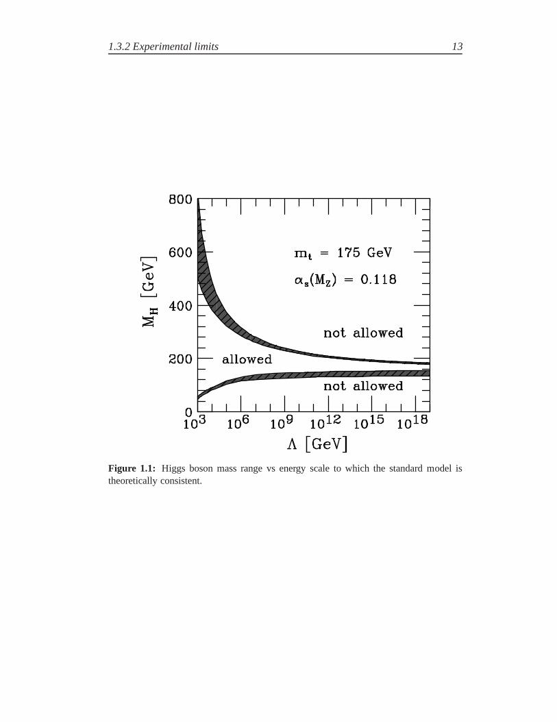
In addition to understand the origin of particles mass, the existence of Higgs bosonis fundamental even to guarantee the renormalizability of electro-weak theory. Byrequiring that the theory wold be renormalizable only at lowenergy (Λ ∼ 1 TeV),the possible Higgs boson mass interval ranges about7 GeV to about103 GeV. Theallowed mass interval becomes narrower if we require that the standard modelwould be consistent up to energyΛ. For a quark top massmt equal to 175 GeV,the allowed values of Higgs boson mass, as function of the energy Λ, are showedin figure1.1.
1.3.2 Experimental limits
The precision reached on the measures of electro-weak observables by the experi-ments with e+- e- collisions amounts to about fractions of percent. These measure-ments indirectly impose limits to Higgs boson mass. The results of direct Higgssearch at LEP experiments fix the lower mass limits tomH > 114.1GeV/c2 with
1.3.2 Experimental limits 13
Figure 1.1: Higgs boson mass range vs energy scale to which the standard model istheoretically consistent.

14 The standard model of elementary particles
95 % confidence level. After the precise measurements of top quark mass (equalto 171.2 ± 2.1 GeV [5]) made at Tevatron experiments, the observables of thestandard model can be written as function of the Higgs boson mass only. Thefit performed to the measured observables, leaving the HiggsmassmH as freeparameter has aχ2 with a minimum atmH = 85 GeV and an upper limit atmH < 212 GeV with 95 % confidence level (this result is showed in Figure1.2).
Figure 1.2: Change of∆χ2 of SM observables as a function of Higgs boson mass. Theyellow band is the mass region excluded at LEP by direct searches.
Finally, data collected from experimentsD0 and CDF at Tevatron (proton -antiproton collision with a center of mass energy equal to 1.96 TeV) allow toexclude, with 95% confidence level, the mass range between 163 and 166 GeV/c2
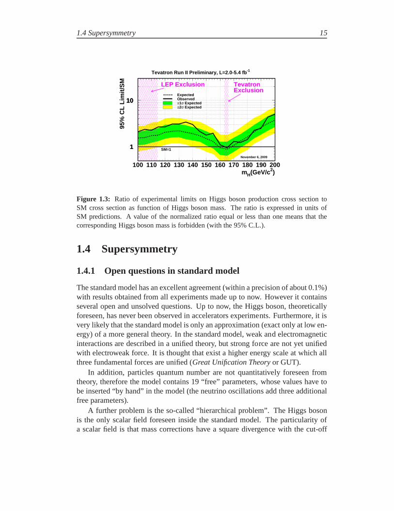
[6] [7]. A summary of allowed and excluded mass ranges is showed in figure1.3:the variable used to discriminate over allowed and forbidden regions for Higgsmass is the ratio between the number of signals recorded (as function of massmH ) and the number of signal expected in the background only hypothesis [8].
1.4 Supersymmetry 15
1
10
100 110 120 130 140 150 160 170 180 190 200
1
10
mH(GeV/c2)
95%
CL
Lim
it/S
M
Tevatron Run II Preliminary, L=2.0-5.4 fb -1
ExpectedObserved±1σ Expected±2σ Expected
LEP Exclusion TevatronExclusion
SM=1
November 6, 2009
Figure 1.3: Ratio of experimental limits on Higgs boson production cross section toSM cross section as function of Higgs boson mass. The ratio isexpressed in units ofSM predictions. A value of the normalized ratio equal or lessthan one means that thecorresponding Higgs boson mass is forbidden (with the 95% C.L.).
1.4 Supersymmetry
1.4.1 Open questions in standard model
The standard model has an excellent agreement (within a precision of about 0.1%)with results obtained from all experiments made up to now. However it containsseveral open and unsolved questions. Up to now, the Higgs boson, theoreticallyforeseen, has never been observed in accelerators experiments. Furthermore, it isvery likely that the standard model is only an approximation(exact only at low en-ergy) of a more general theory. In the standard model, weak and electromagneticinteractions are described in a unified theory, but strong force are not yet unifiedwith electroweak force. It is thought that exist a higher energy scale at which allthree fundamental forces are unified (Great Unification Theoryor GUT).
In addition, particles quantum number are not quantitatively foreseen fromtheory, therefore the model contains 19 “free” parameters,whose values have tobe inserted “by hand” in the model (the neutrino oscillations add three additionalfree parameters).
A further problem is the so-called “hierarchical problem”.The Higgs bosonis the only scalar field foreseen inside the standard model. The particularity ofa scalar field is that mass corrections have a square divergence with the cut-off

16 The standard model of elementary particles
energyΛ2, instead all other divergences are proportional tologΛ2. This leadsto the divergence of the Higgs mass. This problem can be resolved if the Higgsboson is embedded in a supersymmetric theory.
1.4.2 Supersymmetry
The supersymmetric theory (so-calledSUSY) is one of the most promising ex-tension of the standard model and will be, therefore, one of the most importantresearch area for ATLAS and the other LHC experiments. Supersymmetry is thelargest extension of the Lorentz group and starts from the existence of a symmetrybetween fermions and bosons. For each particle with integerspin, there must ex-ist a particle with the same internal quantum numbers, but with half-integer spin(and, vice versa, for each particle with half integer spin there is a particle thathas integer spin). According to the used nomenclature, supersymmetric particlesassociated to the know particles are designed with a tilde over the symbol (for ex-ample “e” ); supersymmetric boson have the same name of standard bosons, butwith the prefixs-; instead supersymmetric fermions are designed with names ofstandard fermions followed by the suffix-ino.The supersymmetric generatorQ, Q satisfies the following commutation rules:
Q, Q = −2γµPµ (1.40)
[Q,P µ] = Q,Q = Q, Q = 0 (1.41)
Q|bosons〉 = |fermions〉 Q|fermions〉 = |bosons〉 (1.42)
(P µ is the momentum operator andγµ are the Dirac matrix).In the minimal extension of standard model (MSSM), each chiral fermionfL,R isassociated to one scalar sfermionfL,R and each massless gauge bosonAµ withtwo elicity states±1 is associated to one massless gaugino with spin−1/2 andelicity ±1. There are also two complex Higgs doublets and their own associ-ated Higgsino. Interactions between supersymmetric particles are obtained fromcorresponding standard interactions by substituting lineof each vertex with super-symmetric particles. Supersymmetry solves the hierarchical problem, due to thefact that bosons and fermions leads to the cancellation of square loop divergences.If the scale of the supersymmetric particles is about 1 TeV, Supersymmetry solvesalso the problem of the unification of fundamental (electro-weak and strong) in-teraction and provide a natural candidate for the dark matter.
Supersymmetry is obviously broken, because superparticles have never beenobserved and many mechanism to broke the symmetry, such asmSugra, are fore-seen by the theory.

1.5 Higgs search at LHC 17
1.5 Higgs search at LHC
1.5.1 Standard Model Higgs
Figure 1.4: Production cross-sections for the SM Higgs boson as a function of its massat LHC, for the expected production processes.
The standard model predicts various possible electroweak mechanisms for theproduction of the Higgs boson. In figure1.4, the expected production cross sec-tions, at LHC design energy for these process are reported asfunction of Higgsboson mass. As could be seen from the figure, the dominant process are thegluon- gluon fusion(gg → H) and thevector boson fusion( qq → qqH ) whose Feyn-man diagrams are drawn in figure1.5. The cross section are numerically small,therefore the Higgs search will be difficult because of the low rate production andthe small signal/background ratio. The searches will be focused on different finalstates according to the possible values of the Higgs mass (figure1.6): in the lowmass region, the most important is the decay channelH → γγ; in the intermedi-ate and high mass regions, the channelH → 4ℓ and, at very high mass, the decayin H → 2ℓνν. In the next sections, it will be reported the details of the decaychannels, classified depending the expected Higgs mass [9]. The branching ratiosof the Standard Model Higgs boson decay channels as a function of Higgs massare reported in figure1.6

18 The standard model of elementary particles
Figure 1.5: Feynman diagrams of the processes mainly contributing to the production ofa SM Higgs boson at LHC: (a) g-g fusion, (b) WW and ZZ fusion.
Figure 1.6: Branching ratios of the Standard Model Higgs boson decay channels as afunction of its mass.
1.5.1 Standard Model Higgs 19
Low-mass Higgs
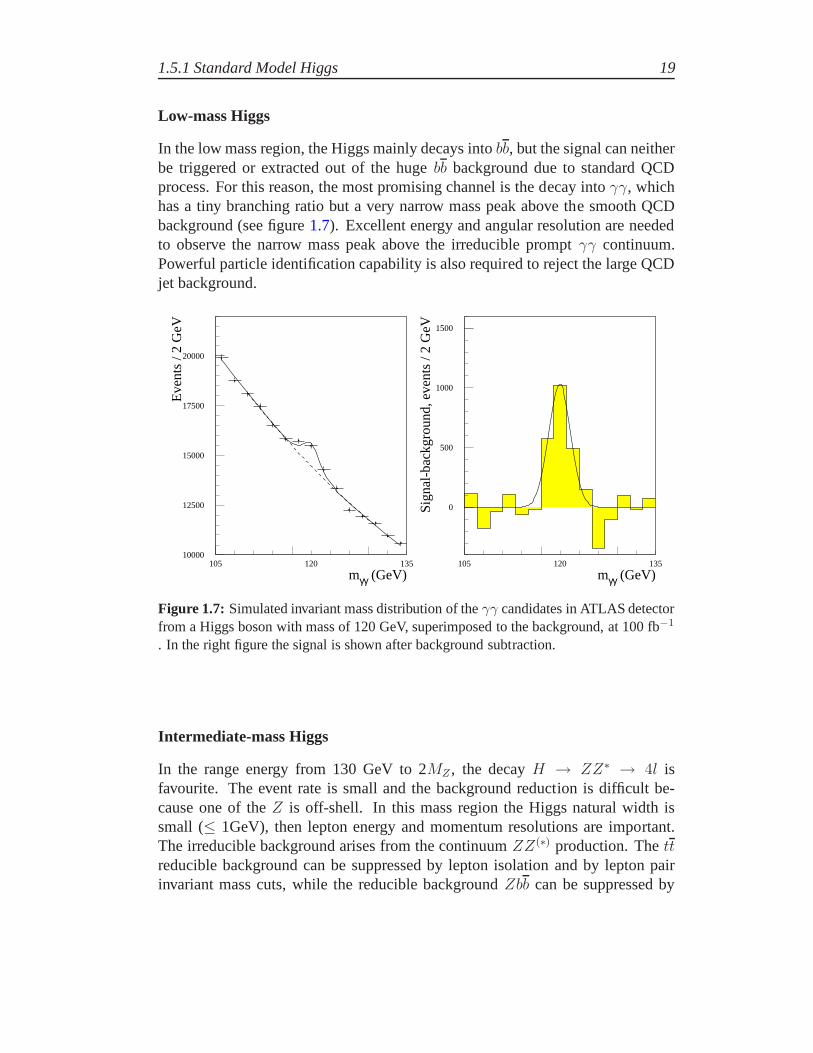
In the low mass region, the Higgs mainly decays intobb, but the signal can neitherbe triggered or extracted out of the hugebb background due to standard QCDprocess. For this reason, the most promising channel is the decay intoγγ, whichhas a tiny branching ratio but a very narrow mass peak above the smooth QCDbackground (see figure1.7). Excellent energy and angular resolution are neededto observe the narrow mass peak above the irreducible promptγγ continuum.Powerful particle identification capability is also required to reject the large QCDjet background.
10000
12500
15000
17500
20000
105 120 135
mγγ (GeV)
Eve
nts
/ 2 G
eV
0
500
1000
1500
105 120 135
mγγ (GeV)
Sig
nal-b
ackg
roun
d, e
vent
s / 2
GeV
Figure 1.7: Simulated invariant mass distribution of theγγ candidates in ATLAS detectorfrom a Higgs boson with mass of 120 GeV, superimposed to the background, at 100 fb−1
. In the right figure the signal is shown after background subtraction.
Intermediate-mass Higgs
In the range energy from 130 GeV to 2MZ , the decayH → ZZ∗ → 4l isfavourite. The event rate is small and the background reduction is difficult be-cause one of theZ is off-shell. In this mass region the Higgs natural width issmall (≤ 1GeV), then lepton energy and momentum resolutions are important.The irreducible background arises from the continuumZZ(∗) production. Thettreducible background can be suppressed by lepton isolationand by lepton pairinvariant mass cuts, while the reducible backgroundZbb can be suppressed by

20 The standard model of elementary particles
Figure 1.8: Simulated 4-leptons invariant mass distribution for various Higgs masses(130, 150 and 170 GeV) with the sum of all backgrounds for 100 fb−1 in ATLAS.
isolation requirements. The signals obtained are very significant (figure1.8): AT-LAS expects signals at the level of 10.3 (7.0), 22.6 (15.5) and 6.5 (4.3) standarddeviation respectively forMH = 130, 150, and 170 GeV in 100 fb−1 (30 fb−1).
The decayH → WW (∗) → l+νl−ν can provide valuable information in themass region around 170 GeV. The dominant background arises from the produc-tion ofW pairs surviving the cuts used to remove thett background.
High-mass Higgs
The “golden” decay modeH → ZZ → 4l has a signal excess of six standarddeviation over a wide range of Higgs masses from 2MZ to about 600 GeV at 100fb−1.
Electron and muon resolutions and selection cuts are similar as for theZZ∗
channel. As the Higgs mass increases, its width increases and its production ratefalls. Decay channels with larger branching fraction areH → WW/ZZ →ll/νν + jets. The enormousW + jets andZ+ jets background must be reducedtagging on one or two forward jets associated to the boson fusion production.
1.5.2 Supersymmetric Higgs
The Higgs sector of the Minimal Supersymmetric Standard Model (MSSM) fore-sees two charged physical states (H±) and three neutral states (h,H,A). This lead
1.5.2 Supersymmetric Higgs 21
to a large spectrum of possible signals and makes difficult the search of an evi-dence of a supersymmetric Higgs boson [9].All the mass and the coupling constants of Higgs boson can be parametrized interm of the mass of the CP-odd bosonmA and the ratio between the vacuumexpectation value of Higgs doublets, written astanβ. Theoretical and experimen-tal studies ([10], [11]) on the detection of the MSSM Higgs boson at the LHChave selected sets of parameters, for which supersymmetricparticle masses arelarge. This forbids kinetically the Higgs boson decay in SUSY particles. There-fore, will be investigated decay mode accessible also in case of SM Higgs boson:H → γγ, H → bb, H → ZZ → 4l (other possible channels areH/A → tt,A→ Zh,H → hh ). At largetanβ the most probable modes areH/A→ ττ andH/A→ µµ.Instead, if susy particles are enough light, decay mode to supersymmetric parti-cles are allowed [12]. In conclusion, the all range 50-500 GeV andtan β = 1−50should be reachable for the Higgs boson discovery at ATLAS experiment.

22 The standard model of elementary particles
2The ATLAS experiment at Large
Hadron Collider
2.1 The Large Hadron Collider
The Large Hadron Collider (LHC) is the new superconducting proton-proton ac-celerator [13] installed at about 100 m deep below the countryside of Geneva(Switzerland) at the CERN laboratory (“European Organization for Nuclear Re-search”). It is now in its initial operating phase at half designed energy and it ismade by two coaxial rings housed in the 27 km tunnel previously constructed forthe Large Electron Positron Collider (LEP). The accelerator has been designedto provide proton-proton collisions with the unprecedented luminosityL of 1034
cm−2s−1, whereL is given by the formula:
L = fN1N2
4πσxσy
F (2.1)
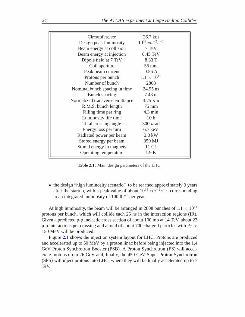
with: N1 andN2 the number of protons per bunch and per beam,f the bunchcollision frequency,σx and σy the parameters characterize the Gaussian beamtransverse profile in the horizontal and vertical directions respectively,F the ge-ometric reduction factor due to the beam crossing angle. In the final operationalconfiguration, the proton beams will collide with an energy of 7 TeV per beam,providing a center-of-mass energy of 14 TeV, which is one order of magnitudehigher than the one reached in any previous collider. The main design parametersof the LHC machine are shown in table2.1.
In addition to the p-p operation, LHC will be able to collide heavy nuclei, e.g.Pb-Pb, with a center-of-mass energy of 2.76 TeV/nucleons atan initial luminosityof 1027 cm−2s−1.
Two main luminosity scenarios are foreseen for the LHC in p-poperation:
• an initial “low luminosity scenario” with a peak luminosityof about 1033
cm−2s−1, corresponding to an integrated luminosity of about 10 fb−1 peryear.
23
24 The ATLAS experiment at Large Hadron Collider
Circumference 26.7 kmDesign peak luminosity 1034cm−2s−1
Beam energy at collision 7 TeVBeam energy at injection 0.45 TeV
Dipole field at 7 TeV 8.33 TCoil aperture 56 mm
Peak beam current 0.56 AProtons per bunch 1.1× 10¹¹
Number of bunch 2808Nominal bunch spacing in time 24.95 ns
Bunch spacing 7.48 mNormalized transverse emittance 3.75µm
R.M.S. bunch length 75 mmFilling time per ring 4.3 minLuminosity life time 10 hTotal crossing angle 300µradEnergy loss per turn 6.7 keV
Radiated power per beam 3.8 kWStored energy per beam 350 MJ
Stored energy in magnets 11 GJOperating temperature 1.9 K
Table 2.1: Main design parameters of the LHC.
• the design “high luminosity scenario” to be reached approximately 3 yearsafter the startup, with a peak value of about 1034 cm−2s−1, correspondingto an integrated luminosity of 100 fb−1 per year.
At high luminosity, the beam will be arranged in 2808 bunchesof 1.1× 10¹¹
protons per bunch, which will collide each 25 ns in the interaction regions (IR).Given a predicted p-p inelastic cross section of about 100 mbat 14 TeV, about 23p-p interactions per crossing and a total of about 700 charged particles with PT >150 MeV will be produced.
Figure2.1 shows the injection system layout for LHC. Protons are producedand accelerated up to 50 MeV by a proton linac before being injected into the 1.4GeV Proton Synchrotron Booster (PSB). A Proton Synchrotron(PS) will accel-erate protons up to 26 GeV and, finally, the 450 GeV Super Proton Synchrotron(SPS) will inject protons into LHC, where they will be finallyaccelerated up to 7TeV.

2.1 The Large Hadron Collider 25
Figure 2.1: Accelerator complex at CERN.

26 The ATLAS experiment at Large Hadron Collider
Figure 2.2: Cross section of a twin-bore magnet for LHC.
The request for very high luminosity excluded the use of a p-p (since an anti-proton beam would require several hours to cool and accumulate anti-protons be-fore injection), consequently, a common vacuum and magnet system for both cir-culating beams was not possible. In fact, to collide two beams of equally chargedparticles requires opposite magnet dipole fields. Therefore, LHC is designed as aproton-proton collider with separate magnetic fields and vacuum chambers in themain arcs and with common pipes, about 130 m long, at the intersection regions(IR), where the experimental detectors are located. The twobeams are separatedalong the IR in order to avoid parasitic collision points.
Since there was not enough space in the LEP tunnel to accommodate twoseparate rings of magnets, LHC uses twin bore magnets, whichconsists of twosets of coils and beam channels within the same mechanical structure and cryostat(see figure2.2). 7 TeV peak beam energy implies a 8.33 T peak dipole field andthe use of a superconducting magnet technology.
Along the accelerator ring, there are four interaction points when proton beamswill collide. In the underground caverns built around thosepoints, the detectorsATLAS, CMS, ALICE and LHCb are installed. ATLAS (in detail described insection2.2) and CMS are general purpose experiments, developed to investigatethe largest range of physics possible, whereas LHCb and ALICE are specializeddetector to investigate specific phenomena.

2.2 The ATLAS experiment at LHC 27
2.2 The ATLAS experiment at LHC
The ATLAS (A Toroidal LHC ApparatuS) experiment is the result of the effortsof a world-wide huge collaboration, composed of about 2800 researchers from173 universities and laboratories of 39 countries. The ATLAS detector layout isshown in figure2.3[14].
Figure 2.3: Overall view of the ATLAS detector displaying various sub-detectors.
The detector has a typical onion structure around the beam pipe. It is com-posed by many different sub-detectors: inner detectors, calorimeter detectors andmuons detectors. Several of these detectors are surroundedby a magnetic fieldgenerated by four magnetic systems.
In the right-handed coordinate system used, the nominal interaction point (IP)is defined as the origin of the coordinate system, the z axis coincides with the beamaxis, the positive x axis points to center of LHC ring from IP and the positive yaxis is oriented upwards. The coordinate system mostly usedare the coordinate z,φ (azimuthal angle measured around beam axis) andθ (polar angle). Thepseudo-rapidity is defined asη = − ln tan(θ/2).
2.2.1 Magnet system
To measure the charged particle momentum, ATLAS uses a magnet system madeof a central solenoid, an air-core barrel toroid and two air-core end-cap toroids.

28 The ATLAS experiment at Large Hadron Collider
The dimensions of the overall system are 26 m of length and 22 mof diameterand it stores an energy of 1.6 GJ [15].
The central solenoid is aligned with the beam axis and provide a 2 T axial mag-netic field for the inner detector. Because the solenoid liesinside the calorime-ter volume, it has been designed to keep the material thickness in front of thecalorimeter as low as possible. In particular, the solenoidwindings and the LiquidArgon calorimeter share a common vacuum vessel.
The barrel toroid is made of eight flat coils assembled radially and symmet-rically. In the windings coils, built with aluminium stabilized Nb/Ti/Cu super-conductor and cooled at 4.5 K, a current of 20.5 kA circulates. The barrel toroidprovides a field of approximately 0.5 T (depending onη) in the region|η| <1.3.
Two end-cap toroids are lined with the central solenoid and generate the mag-netic field required for optimising the bending power in the end-cap regions ofthe muon spectrometer system. Each toroid is made of eight flat coils (rotated by22.5 with respect the barrel toroid coils) located in one large cryostat. The fieldprovided by end-cap toroids is approximately 1 T in the pseudo-rapidity range 1.6< η < 2.7. The geometry of the magnet coils system is schematizedin figure2.4.
Figure 2.4: Geometry of magnet windings and tile calorimeter steel.
2.2.2 Inner detector
The ATLAS Inner Detector (ID) [16, 17] is contained in a cylinder about 7 m longand with radius of 1.15 m, within a solenoidal magnetic field of 2 T. The goal of

2.2.2 Inner detector 29
the ID is to provide a hermetic and robust, in the very high rate environment ofthe LHC accelerator, pattern recognition, an excellent momentum resolution and ameasure of primary and secondary vertexes. For all those purposes, a tracker sys-tem consisting of three independent and complementary sub-detectors (from innerto outer radii silicon pixels, silicon strips and straw tube) has been developed.
Envelopes
Pixel
SCT barrel
SCT end-cap
TRT barrel
TRT end-cap
255<R<549mm|Z|<805mm
251<R<610mm810<|Z|<2797mm
554<R<1082mm|Z|<780mm
617<R<1106mm827<|Z|<2744mm
45.5<R<242mm|Z|<3092mm
Cryostat
PPF1
CryostatSolenoid coil
z(mm)
Beam-pipe
Pixelsupport tubeSCT (end-cap)
TRT(end-cap)
1 2 3 4 5 6 7 8 9 10 11 12 1 2 3 4 5 6 7 8
Pixel
400.5495
580
650749
853.8934
1091.5
1299.9
1399.7
1771.4 2115.2 2505 2720.200
R50.5R88.5
R122.5
R299
R371
R443R514R563
R1066
R1150
R229
R560
R438.8R408
R337.6R275
R644
R1004
2710848712 PPB1
Radius(mm)
TRT(barrel)
SCT(barrel)Pixel PP1
3512ID end-plate
Pixel
400.5 495 580 6500
0
R50.5
R88.5
R122.5
R88.8
R149.6
R34.3
Figure 2.5: Schematic view of a quarter section of the ATLAS Inner Detector.
Silicon pixels [18] are arranged on three coaxial layers in the barrel region andon end-cap three disk (on each side), in total, 1744 pixel modules are installed.The fine granularity (10µm in R − φ plane and 115µm in z) allows to havethree high precision points for pattern recognition near the interaction region and,therefore, to reconstruct primary and secondary particlesdecay vertex.
The Silicon Strips detector (SCT) is made by four layers in barrel region andnine wheels for each end-cap. There are a total of 15912 sensors with 768 stripsof 12 cm length per sensor, with a pitch of 80µm. The detector has an intrinsicresolution of 17µm (in R − φ plane) and of 580µm (in z) and provides at leastfour precision measurements for each track.
The Transition Radiation Tracker (TRT) is made of polyamidedrift (straw)tubes of 4 mm diameter interleaved with transition radiation material. It enhancesthe pattern recognition with an average of 36 point per trackand improves themomentum resolution, without introducing a large amount ofmaterials in front ofthe calorimeter. By detecting the transition radiation it can discriminate and reject

30 The ATLAS experiment at Large Hadron Collider
electrons and pions. TRT tubes (which have an intrinsic resolution of 130µm)are parallel to beam pipe in barrel region and arranged in 16 disks in the end-capregions.
2.2.3 The calorimeter system
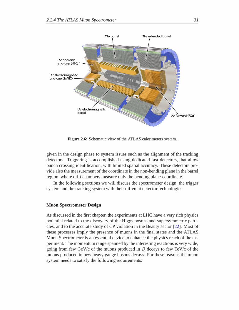
The ATLAS calorimeters are crucial for the reconstruction of the most impor-tant physics channels. In particular, high accuracy on the measurements andidentifications of electrons and photons and a full coveragehadronic calorime-try, for accurate jet and missing transverse energy measurement, are fundamental.The ATLAS calorimeter system is composed of an Electromagnetic Calorime-ter, a Hadronic Calorimeter and a Forward Calorimeter [19, 20]. Figure 2.6 re-ports a general view of ATLAS calorimeters. The electromagnetic calorimeteris separated in a barrel component (η<1.475) and in two end-cap components(1.375<η<3.2) and is constituted of a sampling lead-liquid argon detector, withaccordion shaped kapton electrodes and lead absorber plates. Major physicalrequirements for the detector are a largest possible acceptance, a good electronreconstruction and an excellent energy resolution in a large range (10-300 GeV).
The hadronic calorimeter is composed of:
Tile calorimeter Is the outer part of the system, separated in barrel and end-capregions. It uses steel as absorber and scintillating tiles as the active material.
LAr hadronic end-cap calorimeter Is made of two independent wheels per end-cap and uses the copper-liquid argon sampling technique with flat plate ge-ometry and GaAs preamplifiers in argon.
LAr forward calorimeter The FCal is approximately 10 interaction lengths deepand consists of three modules in each end-cap: the first, madeof copper, isused for electromagnetic measurements, while the other two, made of tung-sten, measure the energy of hadronic interactions.
2.2.4 The ATLAS Muon Spectrometer
The ATLAS Muon Spectrometer [21] design, based on a system of three largesuperconducting air core toroids, was driven by the need of having a very highquality stand-alone muon measurement, with large acceptance both for muon trig-gering and measuring, in order to achieve the physics goals discussed in the firstchapter.
Precision tracking in the Muon Spectrometer is guaranteed by the use of highprecision drift and multi-wire proportional chambers. Great emphasis has been
2.2.4 The ATLAS Muon Spectrometer 31
Figure 2.6: Schematic view of the ATLAS calorimeters system.
given in the design phase to system issues such as the alignment of the trackingdetectors. Triggering is accomplished using dedicated fast detectors, that allowbunch crossing identification, with limited spatial accuracy. These detectors pro-vide also the measurement of the coordinate in the non-bending plane in the barrelregion, where drift chambers measure only the bending planecoordinate.
In the following sections we will discuss the spectrometer design, the triggersystem and the tracking system with their different detector technologies.
Muon Spectrometer Design
As discussed in the first chapter, the experiments at LHC havea very rich physicspotential related to the discovery of the Higgs bosons and supersymmetric parti-cles, and to the accurate study of CP violation in the Beauty sector [22]. Most ofthese processes imply the presence of muons in the final states and the ATLASMuon Spectrometer is an essential device to enhance the physics reach of the ex-periment. The momentum range spanned by the interesting reactions is very wide,going from few GeV/c of the muons produced inB decays to few TeV/c of themuons produced in new heavy gauge bosons decays. For these reasons the muonsystem needs to satisfy the following requirements:

32 The ATLAS experiment at Large Hadron Collider
• a transverse-momentum resolution of few percent in the lowpT region. Thislimit is set by the requirement to detect theH → ZZ∗ decay in the muonchannel with high background suppression;
• at the highestpT the muon system should have sufficient momentum reso-lution to give good charge identification forZ
′ → µ+µ− decay;
• a pseudo-rapidity coverage| η | < 3. This condition guarantees a gooddetection efficiency for high-mass objects decaying into muons with all ofthem within the acceptance region;
• a hermetic system to prevent particles escaping through detector cracks;
• a 3-dimensional measurement of spatial coordinates;
• a low rate of both punch-through hadrons and fake tracks;
• a trigger system for almost all physics channels. For B physics a maximalcoverage and efficiency for muons with transverse momentum down to 5GeV is required.
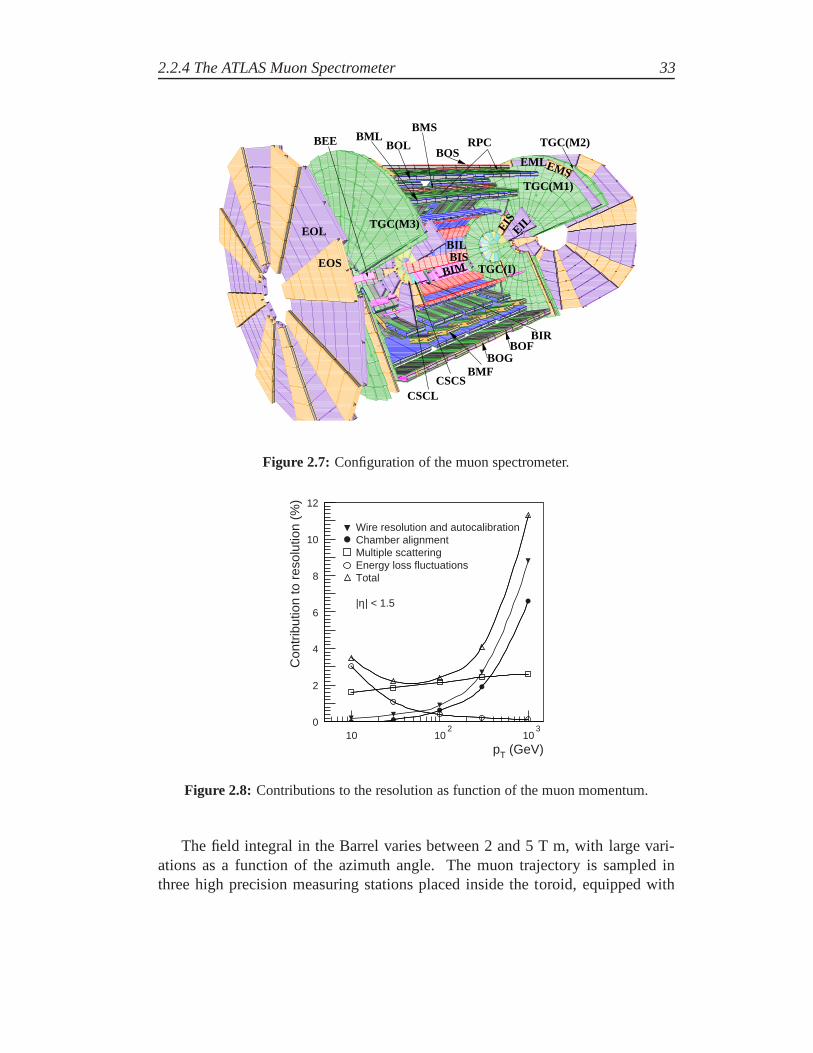
The spectrometer design has been optimized to reach a high resolution androbust stand-alone muon identification and it is illustrated in figure2.7.
Figure2.8shows the different contributions to the muon transverse momentumresolution.
For momenta below 10 GeV/c, the energy loss fluctuation, for muons crossingthe calorimeters, limits the resolution to about 6-8%. The multiple scattering inthe materials limits the resolution to about 2%. While, for higher momenta, theintrinsic spatial accuracy of the chambers and the knowledge of their calibrationand alignment give the largest contribution to the resolution. At 1 TeV/c momen-tum muon is measured with 10% resolution, which was one of the more stringentrequirements on the spectrometer design.
Muon momentum resolution at low momenta (below 100 GeV/c) can be im-proved by using a combined reconstruction of the muon trajectory exploiting alsothe inner tracker measurements. In this case the Muon Spectrometer is usedmainly for the identification of the muon. In figure2.9 the stand-alone and thecombined momentum resolutions are combined as a function ofthe transversemomentum in the region| η |< 1.1. In ATLAS the muon momentum is measuredwith a precision of about 4% up to 250 GeV/c.
The spectrometer is divided into three regions: the Barrel,covering the rapid-ity region| η |≤ 1 and two End-Caps, covering the rapidity regions1 <| η |< 2.7.In the Barrel, the toroidal field is produced by eight very large superconductingcoils arranged in a open geometry (figure2.10).
2.2.4 The ATLAS Muon Spectrometer 33
BIL
BIM
RPC
EIL
EOS
EOL
EMLEMS
BOL
CSCLCSCS
BEE
BIS
BMF
BOS
BMSBML
EIS
BIRBOF
BOG
TGC(M3)
TGC(M1)
TGC(M2)
TGC(I)
Figure 2.7: Configuration of the muon spectrometer.
0
2
4
6
8
10
12
10 102
103
pT (GeV)
Con
trib
utio
n to
res
olut
ion
(%)
Wire resolution and autocalibration Chamber alignment Multiple scattering Energy loss fluctuations Total |η| < 1.5
Figure 2.8: Contributions to the resolution as function of the muon momentum.
The field integral in the Barrel varies between 2 and 5 T m, withlarge vari-ations as a function of the azimuth angle. The muon trajectory is sampled inthree high precision measuring stations placed inside the toroid, equipped with

34 The ATLAS experiment at Large Hadron Collider
Figure 2.9: Stand-alone and combined fractional momentum resolution as a function ofthe transverse momentum.
Figure 2.10: The eight barrel toroid magnets photographed in November 2005 during thedetector installation phase.
Monitored Drift Tubes (MDT, see section2.2.4) and arranged in three cylindri-cal layers around the beam axis. Each station measures the muon positions witha precision of about 50µm in the bending plane. In the two outer stations ofthe Barrel spectrometer, specialized trigger detectors (Resistive Plate Chambers,

2.2.4 The ATLAS Muon Spectrometer 35
RPCs) are present. In the middle station two layers, each comprising two RPCdetectors (RPC doublet), are used to form a low-pT trigger (pT > 6 GeV/c). Inthe outer station only one layer with one RPC doublet is used to form the high-pT
trigger (pT > 10 GeV/c) together with the low-pT station. RPCs measure boththe bending and non-bending coordinate in the magnetic field. Trigger formationrequires fast (< 25 ns) coincidences pointing to the interaction region bothin thebending and non-bending planes.
In the End-Cap regions, two identical air core toroids are shown in figure2.11and are placed on the same axis of the barrel toroid (corresponding to the beamdirection).
Figure 2.11: View of the ATLAS Cavern with the EndCap Magnets in place (July 2007).
The measurement of the muon momentum in the End-Cap region isaccom-plished using three stations of chambers mounted to form three big disks called‘wheels’. These are located normal to the beam direction, and measures the angu-lar displacement of the muon track when passing in the magnetic field (the toroids

36 The ATLAS experiment at Large Hadron Collider
are placed between the first and the second tracking stations).In the End-Cap regions the toroids volume are not instrumented and a sagitta
measurement is not possible but an angular measurement is performed. MDTchambers are used for precise tracking in the full angular acceptance, with theexception of the inner station where the region 2< | η | < 2.7 is equipped withCathode Strip Chambers (CSC, see section2.2.4) which exhibit a smaller occu-pancy. The CSCs have spatial resolution in the range of 50µm.
The trigger acceptance in the End-Caps is limited to| η | < 2.4 where ThinGap Chambers (TGC, see section2.2.5) are used to provide the trigger. The TGCsare arranged in two stations: one made of two double gap layers, used for the lowpT trigger, and one made of a triple gap, used in the highpT trigger in conjunctionwith the low pT stations. The highpT station is placed in front of the middleprecision tracking wheel and the lowpT station is behind it. The TGCs providealso the measurement of the second coordinate and for this reason there is a TGClayer also in the first tracking wheel.
Tracking Chambers
Monitored Drift Tubes: MDT
The precision tracking is performed, in almost the whole spectrometer, by theMonitored Drift Tubes (MDTs). The basic detection element is an aluminiumtube of 30 mm diameter and 400µm wall thickness, with a 50µm diameter centralW-Re wire [23]. The lengths of the tubes vary in the spectrometer from 0.9 to 6.2m. In each measuring station (barrel or end-cap), tubes are assembled in twomulti-layers, which are kept separated by a rigid support structure (spacer frame)that provides accurate positioning of the drift tubes with respect to each other andsupport to the components of the alignment system (see figure2.12).
Multi-layers are made of 3 or 4 tube layers, with four-layer chambers beingused in the inner stations. The mechanical accuracy in the construction of thesechambers is extremely tight to meet the momentum resolutionrequirements ofthe spectrometer. Using an X-Ray Tomography [24], which measure the wireposition with an accuracy of less than 5µm, the precision in wire position in-side a chamber has been checked to be higher than 20µm r.m.s. The requiredhighpT resolution crucially depends also on the single tube resolution, defined bythe operating point, the accurate knowledge of the calibration and the chambers’alignment.
The MDT chambers use a mixture of Ar-CO2 (93% – 7%), kept at 3 bar ab-solute pressure, and operate with a gas gain of 2×10⁴. These parameters werechosen in order to match the running condition of the experiment: the MDTs cansustain high rates without ageing effects [25], and with little sensitivity to space

2.2.4 The ATLAS Muon Spectrometer 37
Figure 2.12: Scheme of a Monitored Drift Tube chamber.
charge. The single tube resolution is below 100µm for most of the range in driftdistance, and the resolution of a multi-layer is approximately expected equal to 50µm.
In order to take advantage of such tracking accuracy, covering a surface perchamber up to 10 m2, an extremely accurate mechanical construction is needed.Furthermore, precise monitoring of the operating conditions is required for bestperformance. Among these issues, very important is an excellent alignment sys-tem that enables the monitoring of the position of the different chambers in thespectrometer with a precision higher than 30µm. Regarding this system, the alu-minium frame supporting the multi-layers is equipped with RASNIK [26] opticalstraightness monitors. These monitors are formed by three elements along a viewline: a laser that illuminates a coded target mask at one end,a lens in the mid-dle and a CCD (Charged Coupled Device) sensors at the other end. This systemprovides a very accurate measurement of the relative alignment of three objects(1 µm r.m.s.) and is used both for checking the chamber deformation (in-planealignment) and the relative displacement of different chamber (projective align-ment). The chambers are also equipped with temperature monitors (in order tocorrect for the thermal expansion of the tubes, and for the temperature of the gas),and with magnetic field sensors (in order to predict the E×B effect on the drifttime).
38 The ATLAS experiment at Large Hadron Collider
0
50
100
150
200
250
300
350
0 2 4 6 8 10 12 14d [mm]
σ d[µm
]
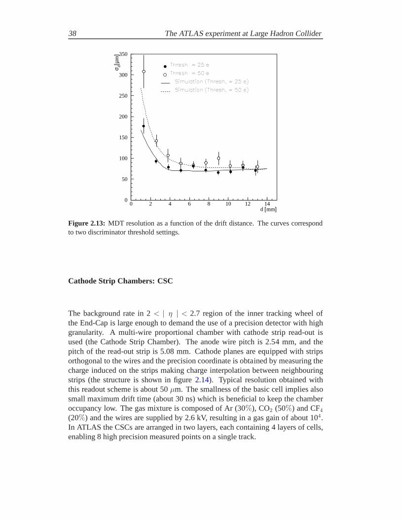
Figure 2.13: MDT resolution as a function of the drift distance. The curves correspondto two discriminator threshold settings.
Cathode Strip Chambers: CSC
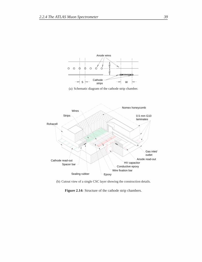
The background rate in 2< | η | < 2.7 region of the inner tracking wheel ofthe End-Cap is large enough to demand the use of a precision detector with highgranularity. A multi-wire proportional chamber with cathode strip read-out isused (the Cathode Strip Chamber). The anode wire pitch is 2.54 mm, and thepitch of the read-out strip is 5.08 mm. Cathode planes are equipped with stripsorthogonal to the wires and the precision coordinate is obtained by measuring thecharge induced on the strips making charge interpolation between neighbouringstrips (the structure is shown in figure2.14). Typical resolution obtained withthis readout scheme is about 50µm. The smallness of the basic cell implies alsosmall maximum drift time (about 30 ns) which is beneficial to keep the chamberoccupancy low. The gas mixture is composed of Ar (30%), CO2 (50%) and CF4(20%) and the wires are supplied by 2.6 kV, resulting in a gas gain of about 104.In ATLAS the CSCs are arranged in two layers, each containing4 layers of cells,enabling 8 high precision measured points on a single track.
2.2.4 The ATLAS Muon Spectrometer 39
Anode wires
Cathode strips
d
d
WS
(a) Schematic diagram of the cathode strip chamber.
Wires
Strips
Rohacell
Cathode read-outSpacer bar
Sealing rubber EpoxyWire fixation bar
Conductive epoxyHV capacitor
Anode read-out
Gas inlet/ outlet
0.5 mm G10 laminates
Nomex honeycomb
(b) Cutout view of a single CSC layer showing the construction details.
Figure 2.14: Structure of the cathode strip chambers.
40 The ATLAS experiment at Large Hadron Collider
2.2.5 Trigger Chambers
The ATLAS physics program demands for a highly flexible trigger scheme withdifferent programmable transverse momentum thresholds. At low luminosity a 6GeV/c threshold for two or more muons is adequate for Beauty physics, whilehigher transverse momentum thresholds (20 GeV/c) will be used for Higgs searchand highpT physics measurements. The muon trigger in ATLAS is organized inthree level. The first level trigger (LVL1), implemented in hardware, uses reduced-granularity data, coming only from the trigger detectors. The second level (LVL2)trigger uses software algorithms exploiting the full granularity and precision datafrom most of the detectors, but examines only the detector region flagged at theLVL1 as containing interesting information (Region of Interest, RoI). The thirdlevel trigger or Event Filter (EF) reconstructs muons applying the same refinedalgorithms of the offline reconstruction in the RoI identified by LVL2. Typicalrates at the three trigger levels are 75 kHz (LVL1), 1 kHz (LVL2) and 100Hz(EF).
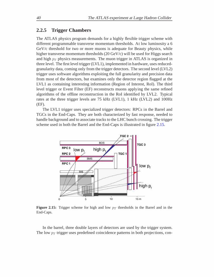
The LVL1 trigger uses specialized trigger detectors: RPCs in the Barrel andTGCs in the End-Caps. They are both characterized by fast response, needed tohandle background and to associate tracks to the LHC bunch crossing. The triggerscheme used in both the Barrel and the End-Caps is illustrated in figure2.15.
Figure 2.15: Trigger scheme for high and lowpT thresholds in the Barrel and in theEnd-Caps.
In the barrel, three double layers of detectors are used by the trigger system.The lowpT trigger uses predefined coincidence patterns in both projections, con-
2.2.5 Trigger Chambers 41
1.8 mm
1.4 mm
1.6 mm G-10
50 µm wire
Pick-up strip
+HV
Graphite layer
Figure 2.16: TGC structure showing positions of anode wires, graphite cathodes, G-10layers and a pick-up strip, orthogonal to the wires.
sidering the RPC middle station only. The momentum resolution is about 20%and is limited mainly by multiple scattering and by fluctuation of the energy lossin the calorimeters. The highpT trigger requires a spatial coincidence patternconsidering the two RPC stations. AtpT of 20 GeV/c the momentum resolutionis about 30% and is limited by the axial length of the interaction region and bymultiple scattering in the central calorimeters. The same logic is applied to thetrigger scheme in the End-Caps. ThepT threshold is defined by the width of thecoincidence patterns and can be programmed. This width depends on the rapidity,and for a 20 GeV/c threshold it varies from about 40 cm in the Barrel to about 5cm in the End-Caps.
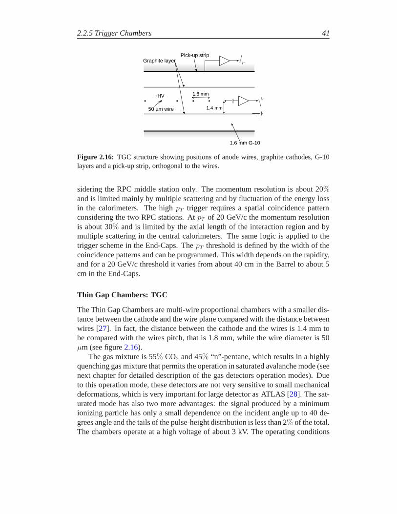
Thin Gap Chambers: TGC
The Thin Gap Chambers are multi-wire proportional chamberswith a smaller dis-tance between the cathode and the wire plane compared with the distance betweenwires [27]. In fact, the distance between the cathode and the wires is 1.4 mm tobe compared with the wires pitch, that is 1.8 mm, while the wire diameter is 50µm (see figure2.16).
The gas mixture is 55% CO2 and 45% “n”-pentane, which results in a highlyquenching gas mixture that permits the operation in saturated avalanche mode (seenext chapter for detailed description of the gas detectors operation modes). Dueto this operation mode, these detectors are not very sensitive to small mechanicaldeformations, which is very important for large detector asATLAS [28]. The sat-urated mode has also two more advantages: the signal produced by a minimumionizing particle has only a small dependence on the incident angle up to 40 de-grees angle and the tails of the pulse-height distribution is less than 2% of the total.The chambers operate at a high voltage of about 3 kV. The operating conditions
42 The ATLAS experiment at Large Hadron Collider
and the electric field configuration provide a short drift time (< 30 ns), enablinga good time resolution. The readout of the signal is done bothfrom the wires(which are grounded together in a variable number, according to the desired trig-ger granularity as a function of the pseudo-rapidity) and from the pick-up stripsplane placed on the cathode. The wires and the strips are perpendicular to eachother enabling the measurement of the orthogonal coordinates, however only thewire signal are used in the trigger logic.
Tests performed at high rate have shown single-plane time resolution of about4 ns with 98% efficiency, providing a trigger efficiency of 99.6% [29].
Resistive Plate Chambers: RPC
The RPC are gaseous detectors providing a typical space-time resolution of 1 cm× 1 ns with digital readout. The active element of the RPC unit is a narrow gas gapformed by two parallel resistive Bakelite plates, separated by insulating spacers.The primary ionization electrons are multiplied in avalanches by a high, uniformelectric field of typically 5 kV/mm. The gas mixture has been chosen in orderto operate in saturated avalanche mode and is composed of three gases: 94.7%C2H2F4, 5% C4H10, 0.3% SF6. Tetrafluoroethane (C2H2F4) has been chosen asmain component since, in addition to satisfy safety requirements, exhibits mod-erately high primary ionization at low operating voltage. Moreover, the mixturecontains isobutane (C4H10) as photons quencher and SF6, in order to reduce theamount of delivered charge and inhibit the streamer development.
Amplification in avalanche mode produces pulses of typically 0.5 pC. Signalsare readout via capacitive coupling by metal strips on both sides of the detectors.In ATLAS, RPC are mounted on MDTs with a mechanical structurethat fix therelative position between chambers. In one readout plane strips (η strips) areparallel to the MDT wires and provide the bending view, whilein the other planestrips (φ strips) are orthogonal to the MTD wires, providing the second-coordinatemeasurement which is also required for the pattern recognition. RPC detectorswill be extensively described in the next chapter.
2.2.6 Trigger and data acquisition system
The 40 MHz proton-proton collision rate of LHC produces a huge amount of read-out signals in ATLAS detector: a trigger system organized onthree distinct levels(Level-1, Level-2andEvent filter) has been implemented to select potentially in-teresting events (see figure2.17).

2.2.6 Trigger and data acquisition system 43
The first level trigger
The first level (L1) trigger (schematized in figure2.18) is implemented on detectorwith custom made electronics board and it uses data from calorimeters and muontrigger chambers.The calorimeter trigger uses reduced granularity informations from all the calorime-ters and searches electrons, photons, jets with high ET or events in which there isa large Emiss
T and a large total transverse energy. The trigger algorithm is basedon the multiplicity of hits from clusters found in the calorimeters and from globalenergy deposition.The level 1 muon trigger uses signals of muon trigger chambers RPC and TGC andsearches for coincidence of hits in trigger station consistent with high-pT muonscoming from interaction point. There are six independentlyprogrammable pTthresholds. Information from all muon trigger sectors are combined by the MuonCentral Trigger Processor Interface (MUCTPI).Informations from calorimeter and muon triggers are combined by the CentralTrigger Processor (CTP) which makes the overall L1 trigger accept decision. Thedetector read-out system can handle a maximum L1 accept rateof about 100 kHz.
Figure 2.17: General view of three levels of the ATLAS trigger system.
The level-1 trigger must operate with a maximum latency of 2.5 µs and hasto identify without ambiguity the bunch crossing of interest. Data of all detectorschannels are retained in pipeline memories (located on or near the detectors) whilethe trigger decision is being formed. If an event is acceptedby level-1 trigger, theregion of interest(RoI), i.e. the information about the geometry location of triggerobject is delivered to level-2 trigger.

44 The ATLAS experiment at Large Hadron Collider
Figure 2.18: Block diagram of the level-1 trigger. Red, blue and black lines are, respec-tively, the output path to detector front-ends, L2 trigger,and data acquisition system.
High level trigger and data acquisition system
The second level of the trigger uses informations from all the subdetectors withfull granularity and precision, in the regions of interest defined by level-1 trigger(in this way the amount of data analyzed is about 2% of the total). The level-2 trigger has an average event processing time of about 40 ms and reduces thetrigger rate to approximately 3.5 kHz.
After that, all event data (associated with a given event) are collected and as-sembled in a formatted structure by thesub farm input(SFI) application. Builtevents are processed by the event filter processing farm. In this step, unlike theL2 trigger, the standard ATLAS analysis and reconstructionprogram is used. Inthis final state, the event rate is reduced to roughly 200 Hz and selection proce-dure has an average event processing time of about four seconds. Data of eventswhich passed the event filter selection criteria are received by theevent filter out-put nodes(SFO) and are written on files located on CERN central data recordingfacility. Data are separated on variousstreamsand written on different files de-pending of the trigger signature (e.g. muons stream, minimum bias stream, etc.).Special streams are thecalibration streamand the express stream. The calibra-tion stream is not recorded at the end of the full trigger chain but at level-2 stepand it is used for detector calibration. The express stream contains a subset ofthe events selected by event filter (in fixed percentage for every streams) and itis reconstructed and analysed promptly as soon as SFO closesthe data files ondisk. This allows to have a quickly feedback of the quality ofdata taken and thedetector status.

3ATLAS RPC trigger chambers
3.1 Resistive Plate Chambers
Resistive Plate Chambers (RPC) have been developed in 1981 by R. Santonico andR. Cardarelli [30]. They are gaseous parallel plate detectors with a time resolutionof ∼ 1 ns, consequently attractive for triggering and Time-Of-Flight applications.
Their main advantages, compared to other technologies, consist in their ro-bustness, construction simplicity and relatively low costof the industrial produc-tion. They are ideal to cover large areas up to few thousand square meters.
RPCs were originally used in streamer mode operation [31], then providinglarge electrical signals, requiring low gain read-out electronics and not stringentgap uniformity. However, high rate applications and detector ageing issues madethe operation in avalanche mode absolutely necessary. Thiswas possible thanksto the use of new highly quenching C2H2F4-based gas mixture instead of the tradi-tional Ar-based mixture and to the development of high gain read-out electronics.
RPC, similarly to Spark Chambers and Parallel Plate Avalanche Chambers,consist of two parallel plate electrodes made with high resistivity material, typi-cally glass or bakelite.
The fundamental processes underlying RPCs are well known. Acharged parti-cle produces free charge carriers in the gas, which drift towards the anode and aremultiplied in a uniform electric field induced by an externalhigh voltage appliedto the electrode plates. The propagation of the growing number of charges inducesan electric signal on the read-out strips, which is amplifiedand discriminated bythe front-end electronics.
The chargeQ0 reaching the electrode surface is locally removed from the elec-trode itself following an exponential law:
Q(t) = Q0e−t/τ with τ = ρε0εr (3.1)
whereρ is the electrode volume resistivity andεr andε0 are the relative permittiv-ity of the resistive material and of the vacuum respectively. τ is defined as the timeneeded by the electrode to get charged again thus recoveringthe initial voltage in
45
46 ATLAS RPC trigger chambers
the gap and varies fromτ ≈ 1 s for glass resistive plates (for which the volumeresistivity isρ ≈ 1012 Ω cm) toτ ≈ 10 ms for plastic-laminated plates (for whichρ ≈ 1010 Ω cm).
3.2 The ATLAS RPC
The RPC gas volumes are made of two parallel bakelite plates,having a volumeresistivityρ≃ 1010±1 Ω cm. They delimit a 2 mm gas gap filled with a gas mixtureat atmospheric pressure. These plates are coated, on the external side, with a thingraphite layer with a surface resistivity ranging from 100 to 300 kΩ/cm2. Thegraphite layer allows to uniformly apply the high voltage tothe electrodes withoutscreening the avalanche signal induced on metal strip readout panels. Moreover,the assembled RPC gas volume is filled with linseed oil, whichis then slowlytaken out. The resulting effect is the deposition of a thin layer of polymerizedoil which smooths the inner bakelite surfaces. This is done in order to reducethe surface imperfections that strongly affect the detector dark current and noisecounting rate. The readout panels are segmented into stripsand simply pressedon the external electrode surface. The readout strips are placed on both sidesof the gap and arranged in perpendicular directions in one side with respect tothe other, allowing to measure thex- andy-coordinate of the ionizing crossingparticle. Strip panels are separated from the graphite coating by an insulatingPET (Polyethylene-Teraphtalate) foil.
A ATLAS RPC unit consists of two independent gas volumes, which are read-out by two orthogonal sets of pick-up strips (see bottom picture of figure3.1).
Two detector layers of one RPC units are interleaved with three support pan-els. The support panels are made of a light-weight paper honeycomb and are heldin position by a solid frame of aluminium profiles. Two external support panelsinterconnected by the aluminium profiles give the required stiffness to the cham-ber.
The RPC units, with the exception of the BMS units (see next section for thenomenclature), have a length in the transverse (φ) direction exceeding the maxi-mum length (3200 mm) of the available bakelite. For this reason the gas volumesare divided in two segments along theφ direction with a 9 + 9 mm inefficient re-gion between the two edge frames. The readout-strip panels are also segmented inthe (φ) direction, including the case of the BMS chambers, in orderto get an ho-mogeneous trigger scheme for all chamber types. This gas volume segmentationreduces theη-strips time jitter by a factor of two.
Most of the RPC trigger chambers are made of two units. The twounits form-ing a chamber have an overlap region of 65 mm to avoid dead areas for curvedtracks (see upper picture of figure3.1). Several RPC trigger chambers are made

3.2.1 Readout panels and front-end electronics 47
of one unit only.
Figure 3.1: The cross-section of an ATLAS RPC chamber made of two units with twodetection layers.
All standard RPC are assembled together with a MDT of equal dimensionsin a common mechanical support structure: an example of the resulting layout isshown in figure3.2. A number of small RPC chambers (special RPC‘s) are notpaired with MDT‘s. These RPC’s are located around the magnetribs and in thefeet region, where MDT‘s cannot be installed because of lackof space. RPC‘s,requiring less space than MDT’s, are used in these regions tokeep the triggeracceptance loss to a minimum.
3.2.1 Readout panels and front-end electronics
A RPC detector operating in avalanche mode produces signalsof 5 ns full widthat half-maximum with a time jitter of 1.5 ns while on the efficiency plateau. Topreserve this high time precision, the pick-up strips must be high quality trans-mission lines with low attenuation and terminated at both ends with their charac-teristic impedance. The layout of a readout strip panel is shown in figure3.3. Thereadout strips have a pitch of 25-35 mm and they are placed on aPET foil gluedon a rigid polystyrene plate. The polystyrene plate is covered on the outside byan other foil PET and a copper sheet as ground reference. The strips are separatedby a 2 mm gap with a 0.3 mm ground strip at the center to improve decoupling.This sandwich structure creates an impedance of about 25Ω for the strips, slightly

48 ATLAS RPC trigger chambers
Figure 3.2: A RPC chamber coupled with a MDT drift tube chamber installedin theATLAS detector.

3.2.1 Readout panels and front-end electronics 49
depending on the width. The pick-up strips outside the PET layers are connectedto the front-end electronics.
Figure 3.3: RPC read-out strip panel.
The front-end circuit is a three-stage shaping amplifier followed by a com-parator. It is implemented by an eight-channel GaAs chip which is bonded on aprinted circuit board and reading out eight strips. The frequency response of theGaAs-amplifiers has a maximum at 100 MHz with a 60 MHz bandwidth, welladapted to the rise time of the chamber signals. The front-end electronics inputis coupled to the strips by a transformer integrated on the printed circuit and itmatches the signal polarities ofη-strips andφ-strips, which are opposite to eachother [32] [33].
Theφ-strips front-end output of two adjacent units are wired OR-ed. This isdone to avoid unnecessary granularity and to adapt the RPC readout segmentationto the trigger sector segmentation as will be discussed in section 3.4. Theφ-striplength and the relative time jitter is in average about half theη-strip relative timejitter, giving to theφ-strips a more precise timing.
In order to be used for the trigger, a signal from a RPC has to becomparedwith those in the two other RPC‘s along the path of the particle. This task isaccomplished by an electronic system of fast coincidence units placed on top ofthe chambers. A detailed discussion of the RPC trigger system is given in section3.4.

50 ATLAS RPC trigger chambers
3.3 ATLAS RPC detector layout
The muon detector chambers are arranged such that particlesfrom the interactionpoint traverse three stations of chambers. In the barrel thechambers are arrangedin three concentric cylinders around the beam axis called BI(Barrel Inner), BM(Barrel Middle), and BO (Barrel Outer). RPC planes are installed in the Middleand Outer stations of the Muon Spectrometer always mechanically associated withMDT precision chambers (except for some “special” chambers). Two RPC planesare integrated with MDT in the Middle stations and one RPC plane only in theOuter stations.
The system is subdivided azimuthally into 16 sectors numbered from 1 to 16.The sector number increases in the direction of increasingφ with the number1 corresponding to coordinateφ = 0. The odd sector (called “large sectors”)are located between barrel coils and the even sectors (called “small sectors”) arecovered by the coils (figure3.4).
The naming convention for RPC chambers are than BMS (Barrel Middle Small),BOS(Barrel Outer Small), BML(Barrel Middle Large) and BOL (Barrel OuterLarge), except for sector 12 and 14 where the ATLAS feet are located and thenaming convention is BMF (Barrel Middle Feet) and BOF (Barrel Outer Feet).
In section4.3, will be detailed how the hardware detector granularity is trans-lated in the detector software description and thus in the histograms naming con-vention used in the following of this work.
3.4 ATLAS Barrel Muon Trigger
The trigger algorithm is based on temporal and spatial coincidences of strip be-longing to different RPC planes (see figure3.5). The number of planes is chosenin order to minimize accidental coincidences and optimize the trigger efficiency.To reduce the number of accidental counts, the trigger operates in the bendingcoordinatesη and in the non-bending coordinateφ separately, but the trigger de-cision requires both to be satisfied. The trigger algorithm can be divided into twoparts, respectively called low-pT trigger and high-pT trigger, depending on thevalue of the particle transverse momentum. This distinction was made in order tooptimize the trigger according to the particles curvature and their loss of energythrough the materials.
In case of low-pT tracks, the algorithm uses information generated by the twoRPC planes of the Middle stations (Pivot plane and low-pT plane in figure3.5).In the bending viewη, if a RPC hit is detected in the doublet stripsη of thePivot plane, a fast RPC hit search is made in the doublet strips η of the low-pT
plane. The search is done with a spatial window (coincidencewindow or trigger

3.4 ATLAS Barrel Muon Trigger 51
Figure 3.4: Cross-section of the barrel muon system perpendicular to beam line.
Figure 3.5: The muon barrel trigger algorithm
road) whose center is given by a hypothetical particle with infinite momentum

52 ATLAS RPC trigger chambers
that travels from the point of interaction to the Pivot hit. The width of the windowis programmable and the particles are selected depending onthe pT (a smallerwindow width gives a higher cut inpT ). The relationship between the windowwidth andpT cut is obtained through Monte Carlo simulations for each Pivot strip(see figure3.6).
The trigger system can be programmed up to three windows simultaneously(corresponding to three differentpT threshold values). The transverse momentumfor low pT particles can varies between 5 and 10 GeV. To deal with the cavernbackground generating low-energy particles, the trigger signal is required to berevealed in at least 3 out of 4 layers.
The algorithm in the non-bending viewφ is identical to that described abovefor η view, except that it links togetherφ strips belonging to adjacent chambersrealizing a logical-or. There could be up to three chambers in logical-or, thiscorresponds to the maximum number of chambers alongη that a muon deflectedin the magnetic field can cross. Theφ view logical-or is realized internally by thetrigger and readout electronics and only for low-pT and high-pT planes (see figure3.7). Instead, theφ view wire-or is realized by cabling on the chambers and forall three RPC planes (see figure3.7).
In case of high-pT tracks, the algorithm uses information generated by thehigh-pT plane, requiring at least 1 out of 2 layer and the low-pT trigger pattern.The algorithm used to search for the hit on high-pT plane is quite similar to thatused previously and is based on the coincidence window concept. Again, it ispossible to program up to three coincidence windows at the same time, for variousvalues of the momentum cut. The transverse momentum for high-pT particlesvaries between 10 and 40 GeV.
The system is then able to resolve up 6 windows simultaneously for each view.The trigger algorithms are realized by implementing coincidence matrix betweenthe signals coming from strip of the same view but belonging to different planes.Next paragraph will detail the trigger hardware layout.
3.4.1 Trigger hardware implementation
The differential signals coming from the front-end electronics are sent to an ASIC1 named Coincidence Matrix (CMA). The CMA’s are used to open a time co-incidence window between strips, generate the trigger signal, locate the bunch-crossing and store the data waiting for the level-1 accept (L1A) decision.
Because of the coincidence windows overlapping, a RPC chamber must sendits signals to more than one CMA. For this reason, the output signals from low-pT
and high-pT RPC planes are readout by splitters. The splitters are designed to
1ASIC: Application Specific Integrated Circuit.

3.4.1 Trigger hardware implementation 53
Figure 3.6: Simulated Low-pT trigger event.

54 ATLAS RPC trigger chambers
Figure 3.7: Logical-or and wired-or inφ views along theη direction.

3.4.1 Trigger hardware implementation 55
duplicate the signal and drive more than one CMA. Another task of the splitter isto convert from ECL2 logic to LVDS3 logic the RPC front-end signals. The pivotRPC plane is directly connected to the CMA and a splitter is not required.
The pivot and low-pT RPC planes are readout by 4 CMA’s (2 forη view and 2for φ view ) and mounted on the same trigger box named low-pT PAD. The taskof the low-pT PAD is to take data from the four coincidence matrix and send themto the high-pT PAD.
The high-pT RPC plane signals and the low-pT CMA trigger signals are read-out by 4 high-pT CMA mounted on the high-pT PAD. The high-pT PAD, afterprocessing, sends data and triggers serially via optic fiberto the off-detector elec-tronic, in a room outside the detector. In this room the signals are received by theSector Logic (SL) and the Read Out Driver (ROD) modules. The trigger signalsare processed and shipped to MUCTPI (MUon Central Trigger Processor inter-face), and hence, ultimately, to the CTP (Central Trigger Processor) which has thetask of taking the final trigger decision.
More specifically, the high-pT PAD, through a FPGA4, takes data from the 8CMA, executes the trigger logic between the two views, selects the greater triggerthreshold, solves overlaps and sends outgoing data and trigger signals. Figure3.8 shows the structure of an ATLAS RPC trigger sector. In particular, a PAD,mounted on top of a RPC chamber, occupy half chamber along theφ direction andcontains 4 CMA, which manages to cover an area∆η × ∆φ ≈ 0.2 × 0.2, whichincludes 4 Regions of Interest (RoI). The RoI is the space region in wich the level-1 trigger identify possible interesting events and cover a sector of∆η × ∆φ ≈0.1 × 0.1, while a CMAη covers a sector∆η × ∆φ ≈ 0.1 × 0.2 and a CMAφcovers a sector∆η×∆φ ≈ 0.2× 0.1. On ATLAS there are in total 832 PAD and1664 RoI.
The Sector Logic module collects signals from all PAD’s of the same triggersector (7 PAD’s for large sector, 6 PAD’s for small sectors) and has the task of:
• Resolve trigger overlaps inη and indicate possible overlays with the adja-cent sector.
• Select the muon with the greaterpT threshold and associate it to the trig-gered ROI.
• Select the muon with the second highestpT threshold and associate it to thetriggered ROI.
Once the data triggers were elaborated by the Sector Logic module, they aresent, via LVDS logic, to the MUCTPI, which receives information from all 64
2Emitter-Coupled Logic: is the logic family used for signalscoming from RPC front-end.3Low-Voltage Differential Signaling.4Field Programmable Gate Array

56 ATLAS RPC trigger chambers
Figure 3.8: Segmentation of ATLAS RPC small sector.
barrel Sector Logics and all 144 end-cap Sector Logic. The MUCTPI has the taskof:
• Resolve overlaps between adjacent Sector Logic.
• Select up to seven candidates for all sixpT threshold.
• Read during a time window programmable up to two bunch-crossing (thisin order to set the timing of the system and monitor directly the activity ofthe trigger chambers).
• Align temporally data from different sectors and associatethe right ROI.
The latency time of the trigger data in the MUCTPI should not exceed 8 bunch-crossing. The muon trigger data is then sent to the CTP, whichtogether with thecalorimetry trigger data built-up the final trigger decision.

4RPC Offline Monitoring
The RPC off-line monitoring developed in this thesis coversbasic aspects of theATLAS RPC detector, such as electronics channels and readout strip response,and its standalone tracking capability1. The RPC off-line monitoring is part ofthe ATLAS official software and data processing which are briefly described inSection4.1.1.
In Section4.2 the main purpose and setting of the four software algorithms,which compose the RPC off-line monitoring, are presented. In Section4.3 anoverview of the RPC detector and readout electronics granularity is presented to-gether with the detailed single readout strip and single channel histograms usedfor RPC commissioning with cosmics. In Section4.4 the monitoring of the RPCand MDT signals correlation is presented and in section4.5 is reported the RPCtracking algorithm and its use to evaluate the RPC efficiency.
In Section?? simulated cosmic and commissioning data monitoring plots arecompared, together with the validation of the techniques used to measure the effi-ciency.
4.1 ATLAS software infrastructure
4.1.1 The Athena framework
The ATLAS reconstruction software framework is called Athena [34]. It is usedfor a variety of purposes, including high-level triggering, simulation, reconstruc-tion, monitoring and analysis. Athena provide a skeleton framework in whichusers can embed his/her analysis code.
Athena is an enhanced concrete implementation of a general component-basedarchitecture called Gaudi [35], developed for a wide range of experimental andcomputing applications. The development of Athena software was driven by some
1At the moment of writing the monitoring is not dealing with the RPC LVL1 trigger chainwhere signals from different coincidence matrix are arbitrated, combined in two views, and se-lected by the Pads, the Sector Logic and the MUCTPI (see section3.4).
57
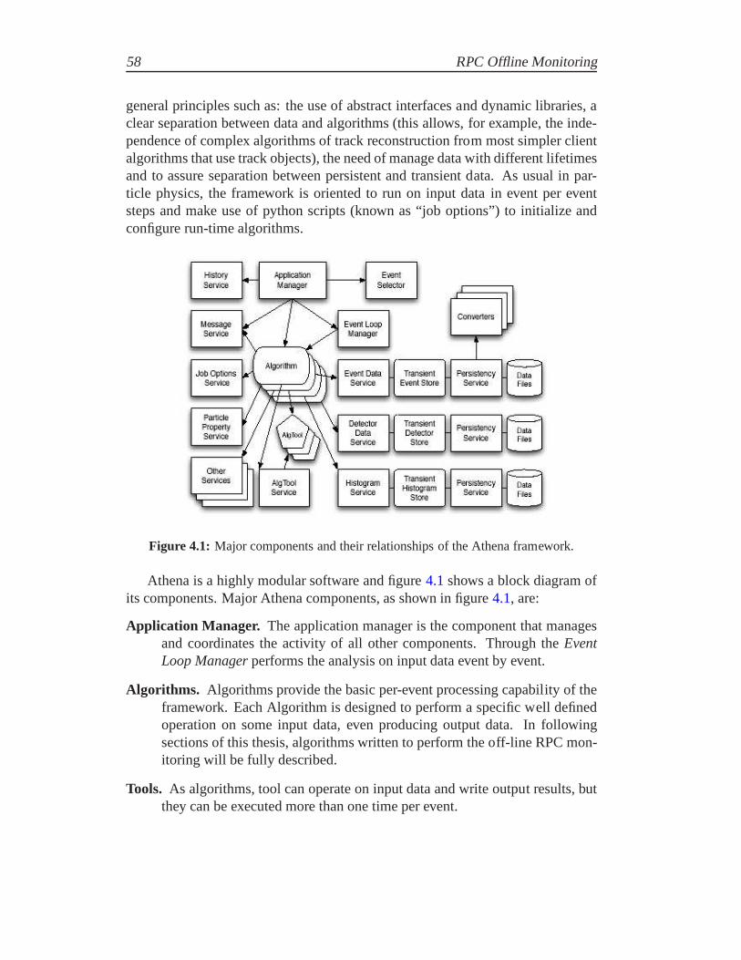
58 RPC Offline Monitoring
general principles such as: the use of abstract interfaces and dynamic libraries, aclear separation between data and algorithms (this allows,for example, the inde-pendence of complex algorithms of track reconstruction from most simpler clientalgorithms that use track objects), the need of manage data with different lifetimesand to assure separation between persistent and transient data. As usual in par-ticle physics, the framework is oriented to run on input datain event per eventsteps and make use of python scripts (known as “job options”)to initialize andconfigure run-time algorithms.
Figure 4.1: Major components and their relationships of the Athena framework.
Athena is a highly modular software and figure4.1shows a block diagram ofits components. Major Athena components, as shown in figure4.1, are:
Application Manager. The application manager is the component that managesand coordinates the activity of all other components. Through theEventLoop Managerperforms the analysis on input data event by event.
Algorithms. Algorithms provide the basic per-event processing capability of theframework. Each Algorithm is designed to perform a specific well definedoperation on some input data, even producing output data. Infollowingsections of this thesis, algorithms written to perform the off-line RPC mon-itoring will be fully described.
Tools. As algorithms, tool can operate on input data and write output results, butthey can be executed more than one time per event.
4.1.2 Data reconstruction process 59
Services.Software components providing specific capabilities needed by algo-rithms.
Transient Data Stores. Data object used by algorithms are managed and orga-nized by specific services depending on data type (event data, detector data,etc.)
Converters. Designed for the conversion of data from raw data to offline formatand from transient to persistent (and vive versa) form. Theyallow algo-rithms code to be independent from the persistency mechanisms.
Selector. Selectors perform selection of events that will be processed.
ATLAS Software has a hierarchical structure: Athena is split in Projectsandthese ones are organized inPackages, a complete collections of projects is iden-tified by an overallreleasenumber. Athena packages are managed in the CMT2
configuration management environment and software code is developed by usingSVN (Subversion) tool.
4.1.2 Data reconstruction process
As explained in section2.2.6, the data read-out by the ATLAS detector (Front-End) are filtered by three levels of on-line triggers: level 1(LVL1), level 2 (LVL2)and Event Filter (EF) [36]. The recorded events are stored into different streamsdepending on purpose (calibrations, physics or monitoring) and trigger hypothe-ses (muons, calorimetric clusters, minimum bias, and so on ...). The “express”stream is a special stream, contains a sample of each other trigger stream and it isanalyzed first to provide a fast feedback of the detector status. A single run is splitin luminosity blockswhich have a fixed duration (five minuts) and are written inseveral files ( of 2 GB size maximum).
Data recorded are in byte stream format (RAW data) and contain only hits ofelectronic read-out channels and information about trigger decisions. Those dataare decoded and reconstructed by running Athena reconstruction process in var-ious steps. First, data are translated from electronic channels to correspondentdetector elements (i.e. read-out strips for RPC), then are reconstructed particlestracks, energy deposits in calorimeter cells, etc. Finally, are identified particles,secondary vertex, etc. Detailed output of the detector reconstruction from RAWdata is written in ESD (Event Summary Data) files, AOD (Analysis Object Data)files, also produced in reconstruction process, contain a summary of the recon-structed event and sufficient information for common analyses. The data file size
2http://www.cmtsite.org/

60 RPC Offline Monitoring
per event changes from 1 MB per event for RAW files to 100 kB per event of AODfiles (for ESD is 500 kB per event).
In parallel with each reconstruction process, off-line monitoring process areperformed.
ATLAS uses a hierarchical analysis model. The reconstruction above de-scribed is run at the CERN computing farm (the Tier-0 centre)on the expressstream (see pag.44) as soon as data are available on disk and after on the differentdata streams.
Data quality is monitored online at the trigger level as wellas offline duringreconstruction. Monitoring histograms are checked by shifters and automaticallyvia the Data Quality Monitoring Framework [37].
In the hierarchical ATLAS analysis model, the first step of reconstruction/monitoringprocess is done at the CERN computer farm called tier-0.
Detector calibrations, alignment, and basic detector operation have to be ver-ified by rapidly reconstructing a smaller subset of the physics events (expressstream). The first express reconstruction occurs as soon as data for a run areavailable and the necessary detector conditions information has been replicated toTier-0, generally within few hours of the start of a run. Additional reconstructioniterations will occur as necessary until the calibrations are approved for full recon-struction. First pass of calibration and alignment should occurs within 24 hoursafter the data has been taken. The obtained constants are then used for the bulkprocessing of the data, once they have been validated by a second re-processingof the express stream.
Data are then distributed to the regional (calledTier-1) and local (calledTier-2) centres for data analysis. The Tier-1 centres are also responsible for data re-processing, i.e re-running reconstruction with improved calibration and alignmentconstants and with improved reconstruction algorithms.
Specialized calibration centers at Tier-2 facilities are also available in order toincrease the statistics and the computer power available for calibration purposes.Specifically, Naples Tier-2 center is devoted to RPC calibrations. The RPC off-line monitor software here described is fully integrated with the Tier-2 calibrationcenter infrastructure.
4.2 RPC off-line monitoring
Inside the general ATLAS off-line monitoring package, RPC monitoring tool hasbeen developed. The RPC monitoring consists of four different algorithms spe-cialized for different aspects of the RPC detector data object:
Electronic channels monitoring Monitoring the detector at the basic level of theread-out electronic channels (that means, for RPC, CMA channels, see sec.

4.2 RPC off-line monitoring 61
3.4.1). It is run on RAW data in the first step of off-line reconstruction andit is focused to check possible problems in read-out hardware 3.
Detector element monitoring It is focused to monitor readout strips (offline iden-tifiers).
RPC-MDT correlation monitoring It verify the correct time and spatial corre-lation between RPCη view strips and MDT tubes.
Track monitoring To explore the tracking capability of RPCs, a track tool thatreconstructs muon tracks by using only RPC signals has been developed,those tracks (that in the following will be calledRPC standalone tracks) areused to evaluate the performance (efficiency and noise) of RPC detector.
The output of the monitoring application are ROOT histograms, that are groupedin folder, one for each of the four algorithms. Further, histograms resultant of eachalgorithm are classified and grouped in different sub-folders according the differ-ent granularity on detector representations and the different application purposes.This classification is described below:
• Commissioning plots. These histograms are related to a single muon sta-tion or to a single trigger tower. They are named according tothe hard-ware layout and used for commissioning. Because there are about 400 RPCchambers installed and by counting an average number of 100 histogramsper chamber,the resulting number of plots is huge and than organized insub-folder according to the station name and Sector Logic number.
In order to reduce the number of histograms during the commissioningphase, where the RPC coverage was limited to a part of the apparatus, andduring normal runs, when single data file have no more than several thou-sands of events, the booking is done only when the very first hit belongingto that plots appear in the event (automatic plot booking). To understandat glance the RPC coverage and simplify the data quality automatic checks,most of these histograms are booked exactly with the correctrange (auto-matic axis range). A hole in these histograms corresponds to a hole in thedetector coverage.
• Sector plots.The monitored quantities are plotted for an entire sector toal-low a fast and comprehensive understanding of the detector response. The
3RPC Level 1 trigger decision quantities are not monitored but only quantities related to it,such as: ‘Pivot’ strips and thresholds causing a local coincidence in a single Coincidence Matrixwhich are readout similarly to raw hits.

62 RPC Offline Monitoring
histograms are organized in sub-folders, each one corresponding to a geo-metrical sector. Similarly to the previous ones, these histograms are bookedautomatically and have automatic axis ranges.
• Overview plots. These histograms are related to the global RPC statusgoing into details and monitoring high level quantities forthe RPC expert.
• Shifter plots. These histograms are intended to be controlled run by run bynon expert shifters. These plots give a global and complete view of the RPCstatus without too many details.
• Side A and C plots.These histograms are used to generate RPC Side A andC data quality flags, which are stored into the so called Condition Databaseas required by the ATLAS experiment. These plots are groupedin sub-folders named‘RPCBA’ and‘RPCBC’, where BA (BC) stands for Barrelside A (C), and produced by the packages RpcRawDataValAlg and RPC-StandaloneTracksMon.
• Readout strip panel summary plots.These histograms are meant to char-acterize exhaustively the detector response in terms of readout panel av-erage quantities such as efficiency, noise, cluster size, timing, occupancyand spatial residuals. These plots are produced by the package RPCStan-daloneTracksMon, where track informations are available,and located inthe sub-folder named‘Summary’. For each geometrical sector and av-erage quantity there is a summary histogram, where each bin correspondsto a readout panel, and a distribution plot filled with the summary plot bincontents.
• Single strip summary plots. These histograms are meant to characterizeexhaustively the detector response with single readout strip granularity interm of the same quantities like the readout panels. These plots are pro-duced by the package RPCStandaloneTracksMon where track informationsare available and located in the sub-folder named‘CoolDB’. For each ge-ometrical sector, detection layer, and average quantity, there is a single stripsummary histogram. Each bin of the histograms corresponds to a readoutstrip.
• Efficiency and noise maps.These histograms are meant to monitor theRPC gas volume response during the lifetime of the experiment in order toperform aging studies. These plots are produced by the package RPCStan-daloneTracksMon, where track informations are available,and located inthe sub-folder named‘RPCRadiography’.
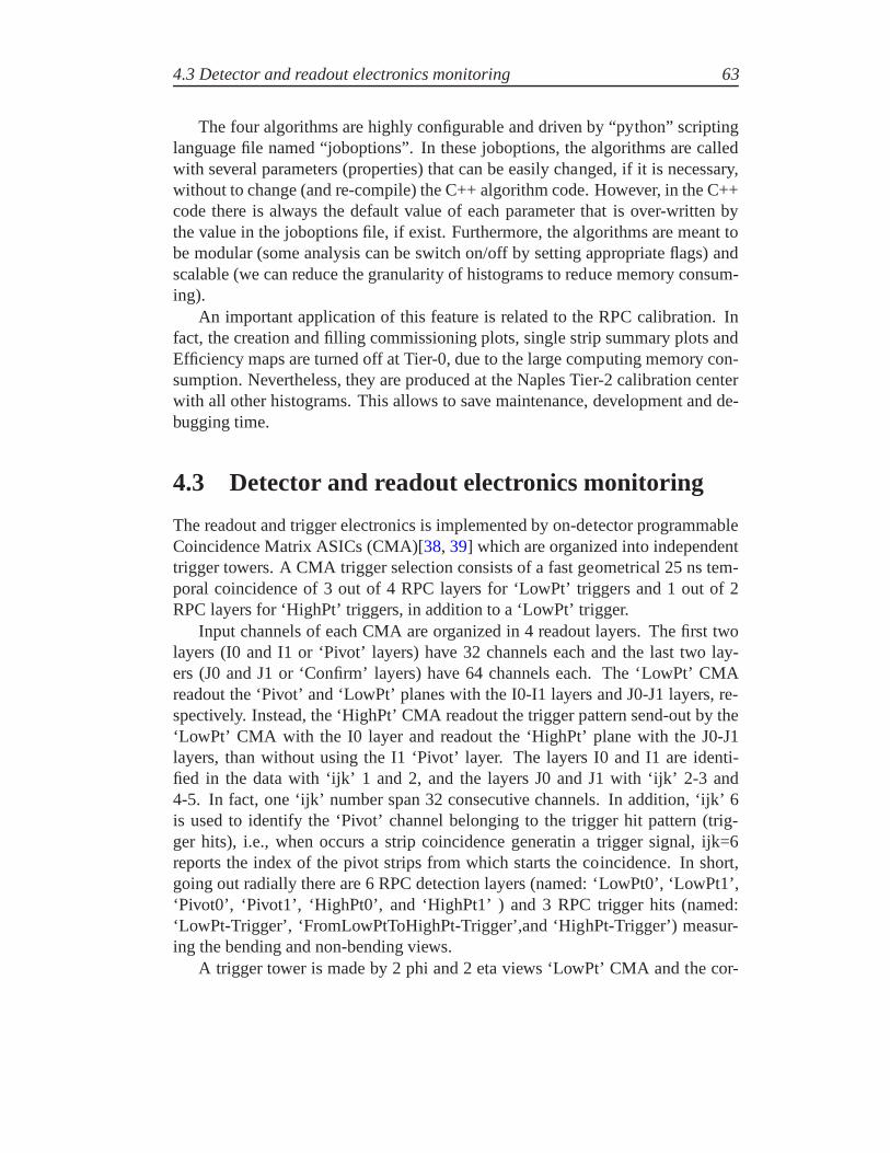
4.3 Detector and readout electronics monitoring 63
The four algorithms are highly configurable and driven by “python” scriptinglanguage file named “joboptions”. In these joboptions, the algorithms are calledwith several parameters (properties) that can be easily changed, if it is necessary,without to change (and re-compile) the C++ algorithm code. However, in the C++code there is always the default value of each parameter thatis over-written bythe value in the joboptions file, if exist. Furthermore, the algorithms are meant tobe modular (some analysis can be switch on/off by setting appropriate flags) andscalable (we can reduce the granularity of histograms to reduce memory consum-ing).
An important application of this feature is related to the RPC calibration. Infact, the creation and filling commissioning plots, single strip summary plots andEfficiency maps are turned off at Tier-0, due to the large computing memory con-sumption. Nevertheless, they are produced at the Naples Tier-2 calibration centerwith all other histograms. This allows to save maintenance,development and de-bugging time.
4.3 Detector and readout electronics monitoring
The readout and trigger electronics is implemented by on-detector programmableCoincidence Matrix ASICs (CMA)[38, 39] which are organized into independenttrigger towers. A CMA trigger selection consists of a fast geometrical 25 ns tem-poral coincidence of 3 out of 4 RPC layers for ‘LowPt’ triggers and 1 out of 2RPC layers for ‘HighPt’ triggers, in addition to a ‘LowPt’ trigger.
Input channels of each CMA are organized in 4 readout layers.The first twolayers (I0 and I1 or ‘Pivot’ layers) have 32 channels each andthe last two lay-ers (J0 and J1 or ‘Confirm’ layers) have 64 channels each. The ‘LowPt’ CMAreadout the ‘Pivot’ and ‘LowPt’ planes with the I0-I1 layersand J0-J1 layers, re-spectively. Instead, the ‘HighPt’ CMA readout the trigger pattern send-out by the‘LowPt’ CMA with the I0 layer and readout the ‘HighPt’ plane with the J0-J1layers, than without using the I1 ‘Pivot’ layer. The layers I0 and I1 are identi-fied in the data with ‘ijk’ 1 and 2, and the layers J0 and J1 with ‘ijk’ 2-3 and4-5. In fact, one ‘ijk’ number span 32 consecutive channels.In addition, ‘ijk’ 6is used to identify the ‘Pivot’ channel belonging to the trigger hit pattern (trig-ger hits), i.e., when occurs a strip coincidence generatin atrigger signal, ijk=6reports the index of the pivot strips from which starts the coincidence. In short,going out radially there are 6 RPC detection layers (named: ‘LowPt0’, ‘LowPt1’,‘Pivot0’, ‘Pivot1’, ‘HighPt0’, and ‘HighPt1’ ) and 3 RPC trigger hits (named:‘LowPt-Trigger’, ‘FromLowPtToHighPt-Trigger’,and ‘HighPt-Trigger’) measur-ing the bending and non-bending views.
A trigger tower is made by 2 phi and 2 eta views ‘LowPt’ CMA and the cor-
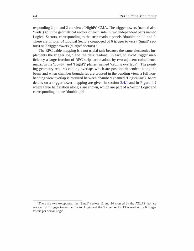
64 RPC Offline Monitoring
responding 2 phi and 2 eta views ‘HighPt’ CMA. The trigger towers (named also‘Pads’) split the geometrical sectors of each side in two independent parts namedLogical Sectors, corresponding to the strip readout panels‘doublet phi’ 1 and 2.There are in total 64 Logical Sectors composed of 6 trigger towers (‘Small’ sec-tors) or 7 trigger towers (‘Large’ sectors)4.
The RPC cable mapping is a not trivial task because the same electronics im-plements the trigger logic and the data readout. In fact, to avoid trigger inef-ficiency a large fraction of RPC strips are readout by two adjacent coincidencematrix in the ‘LowPt’ and ‘HighPt’ planes (named ‘cabling overlaps’). The point-ing geometry requires cabling overlaps which are position dependent along thebeam and when chamber boundaries are crossed in the bending view, a full non-bending view overlap is required between chambers (named ‘Logical-or’). Moredetails on a trigger tower mapping are given in section3.4.1and in Figure4.2where three half station along z are shown, which are part of aSector Logic andcorresponding to one ‘doublet phi’.
4There are two exceptions: the ‘Small’ sectors 12 and 14 crossed by the ATLAS feet arereadout by 3 trigger towers per Sector Logic and the ‘Large’ sector 13 is readout by 6 triggertowers per Sector Logic.

4.3 Detector and readout electronics monitoring 65
Figure 4.2: RPC trigger tower (Pad_n) implementing a projective muon trigger based ona geometrical coincidence between RPC raw hits from ‘LowPt’plane, ‘Pivot’ plane and‘HighPt’ plane. The trigger tower is segmented in four (ROI’s) Region Of Interest’s, thereare exceptions where only oneη CMA is used and the trigger tower have two ROI’s. Thetrigger tower mapping overlap in ‘LowPt’ plane (O1) and ‘HighPt’ plane (O2) betweenadjacent ROI’s inside a trigger tower and between trigger tower (only η overlap insidea trigger tower is shown). The trigger tower makes a ‘Logical-or’ in φ view with thestation nearest to the IP on ‘LowPt’ plane (Lor1) and with thefarthest one or both ones on‘HighPt’ plane (Lor2). The picture shows the “wired-or” (Wor) in φ view of the centralstation.
The RPC readout electronics granularity is translated intothe following fiveinteger parameters:
• sector logic: from 0 to 63.
• pad: from 0 to 6.
• coincidence matrix: from 0 to 7.
• ijk layer: from 0 to 6.
• electronic channel: from 0 to 31.
An electronic channel is translated into one or more readoutstrips by the RPCcabling service.
As already explained in section3, the RPC detector is build from single RPCunits. The RPC planes are made of one or two mechanically independent RPC
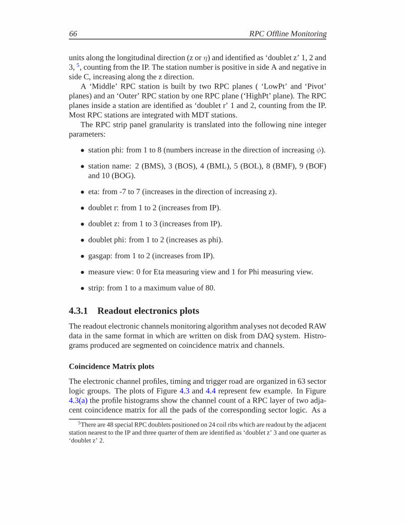
66 RPC Offline Monitoring
units along the longitudinal direction (z orη) and identified as ‘doublet z’ 1, 2 and3, 5, counting from the IP. The station number is positive in sideA and negative inside C, increasing along the z direction.
A ‘Middle’ RPC station is built by two RPC planes ( ‘LowPt’ and‘Pivot’planes) and an ‘Outer’ RPC station by one RPC plane (‘HighPt’plane). The RPCplanes inside a station are identified as ‘doublet r’ 1 and 2, counting from the IP.Most RPC stations are integrated with MDT stations.
The RPC strip panel granularity is translated into the following nine integerparameters:
• station phi: from 1 to 8 (numbers increase in the direction ofincreasingφ).
• station name: 2 (BMS), 3 (BOS), 4 (BML), 5 (BOL), 8 (BMF), 9 (BOF)and 10 (BOG).
• eta: from -7 to 7 (increases in the direction of increasing z).
• doublet r: from 1 to 2 (increases from IP).
• doublet z: from 1 to 3 (increases from IP).
• doublet phi: from 1 to 2 (increases as phi).
• gasgap: from 1 to 2 (increases from IP).
• measure view: 0 for Eta measuring view and 1 for Phi measuringview.
• strip: from 1 to a maximum value of 80.
4.3.1 Readout electronics plots
The readout electronic channels monitoring algorithm analyses not decoded RAWdata in the same format in which are written on disk from DAQ system. Histro-grams produced are segmented on coincidence matrix and channels.
Coincidence Matrix plots
The electronic channel profiles, timing and trigger road areorganized in 63 sectorlogic groups. The plots of Figure4.3 and4.4 represent few example. In Figure4.3(a)the profile histograms show the channel count of a RPC layer oftwo adja-cent coincidence matrix for all the pads of the corresponding sector logic. As a
5There are 48 special RPC doublets positioned on 24 coil ribs which are readout by the adjacentstation nearest to the IP and three quarter of them are identified as ‘doublet z’ 3 and one quarter as‘doublet z’ 2.
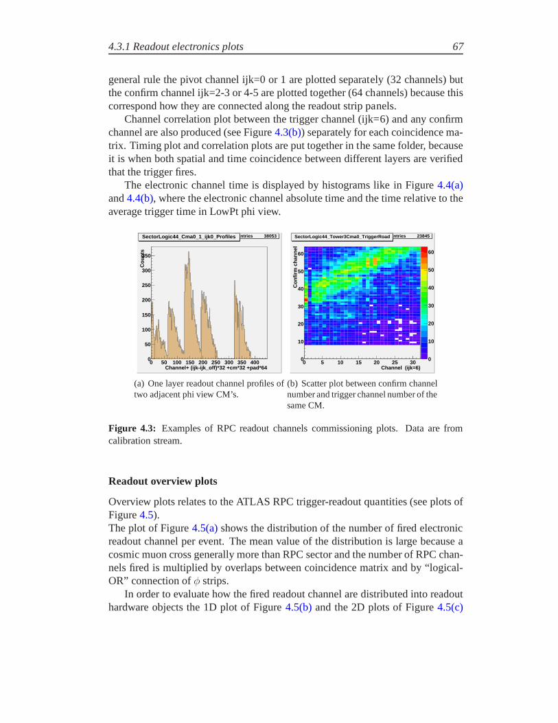
4.3.1 Readout electronics plots 67
general rule the pivot channel ijk=0 or 1 are plotted separately (32 channels) butthe confirm channel ijk=2-3 or 4-5 are plotted together (64 channels) because thiscorrespond how they are connected along the readout strip panels.
Channel correlation plot between the trigger channel (ijk=6) and any confirmchannel are also produced (see Figure4.3(b)) separately for each coincidence ma-trix. Timing plot and correlation plots are put together in the same folder, becauseit is when both spatial and time coincidence between different layers are verifiedthat the trigger fires.
The electronic channel time is displayed by histograms likein Figure4.4(a)and4.4(b), where the electronic channel absolute time and the time relative to theaverage trigger time in LowPt phi view.
Channel+ (ijk-ijk_off)*32 +cm*32 +pad*640 50 100 150 200 250 300 350 400
Cou
nts
0
50
100
150
200
250
300
350
SectorLogic44_Cma0_1_ijk0_Profiles Entries 38053SectorLogic44_Cma0_1_ijk0_Profiles
(a) One layer readout channel profiles oftwo adjacent phi view CM’s.
0
10
20
30
40
50
60
Channel (ijk=6)0 5 10 15 20 25 30
Con
firm
cha
nnel
0
10
20
30
40
50
60
SectorLogic44_Tower3Cma0_TriggerRoad Entries 23845SectorLogic44_Tower3Cma0_TriggerRoad
(b) Scatter plot between confirm channelnumber and trigger channel number of thesame CM.
Figure 4.3: Examples of RPC readout channels commissioning plots. Dataare fromcalibration stream.
Readout overview plots
Overview plots relates to the ATLAS RPC trigger-readout quantities (see plots ofFigure4.5).The plot of Figure4.5(a)shows the distribution of the number of fired electronicreadout channel per event. The mean value of the distribution is large because acosmic muon cross generally more than RPC sector and the number of RPC chan-nels fired is multiplied by overlaps between coincidence matrix and by “logical-OR” connection ofφ strips.
In order to evaluate how the fired readout channel are distributed into readouthardware objects the 1D plot of Figure4.5(b)and the 2D plots of Figure4.5(c)

68 RPC Offline Monitoring
Channel + 32 * ijk0 20 40 60 80 100 120 140 160 180 200 220
Tim
e=bc
Id*8
+tic
ks
0
10
20
30
40
50
60
SectorLogic44_Tower3Cma0_time_vs_channel Entries 27139SectorLogic44_Tower3Cma0_time_vs_channel
(a) Time vs readout channel of a CM.
Channel + 32 * ijk0 20 40 60 80 100 120 140 160 180 200 220
Tim
e=bc
Id*8
+tic
ks
-60
-40
-20
0
20
40
60
SectorLogic44_Tower3Cma0_(time-triggertime)_vs_channel Entries 27139SectorLogic44_Tower3Cma0_(time-triggertime)_vs_channel
(b) Relative time w.r.t average RPC trig-ger time vs readout channel of a CM.
Figure 4.4: Examples of RPC readout channels commissioning plots in ‘RP-CLV1/Profiles/SectorLogic44’ folder: and ‘RPCLV1/TriggerRoad/SectorLogic44’ fold-ers. Data are from calibration stream.
and 4.5(d) count the total number of fired channel per Sector Logic, Pad andCoincidence Matrix. The two bi-dimensional histograms have on the X axis thesector logic and on the Y axis, respectively, the Pad number (from 0 to 7) and theCoincidence Matrix number shifted by eight times the Pad number.
The plots of Figure4.5(e)shows the distribution of the number of trigger hitsper event separated for the two views. The are four of such a plots. Two plots,one shown in Figure4.5(f), display the correlation between trigger hits in Etaand Phi view. Plots showing the correlation between Eta and Phi CoincidenceMatrix trigger hits are also produced. These plots identifyan area called Regionof Interest (RoI).
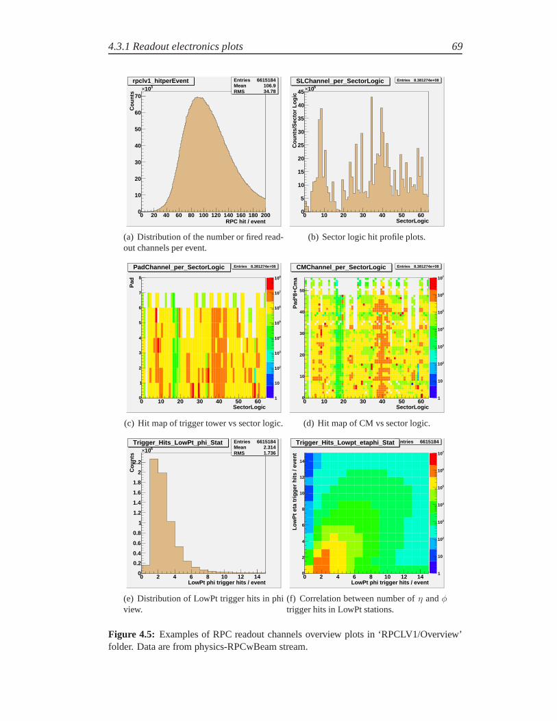
4.3.1 Readout electronics plots 69
RPC hit / event0 20 40 60 80 100 120 140 160 180 200
Cou
nts
0
10
20
30
40
50
60
70
310×rpclv1_hitperEvent Entries 6615184
Mean 106.9RMS 34.78
rpclv1_hitperEvent
(a) Distribution of the number or fired read-out channels per event.
SectorLogic0 10 20 30 40 50 60
Cou
nts/
Sec
tor
Logi
c
0
5
10
15
20
25
30
35
40
45610×
SLChannel_per_SectorLogic Entries 8.381274e+08SLChannel_per_SectorLogic
(b) Sector logic hit profile plots.
1
10
210
310
410
510
610
710
810
SectorLogic0 10 20 30 40 50 60
Pad
0
1
2
3
4
5
6
7
8
PadChannel_per_SectorLogic Entries 8.381274e+08PadChannel_per_SectorLogic
(c) Hit map of trigger tower vs sector logic.
1
10
210
310
410
510
610
710
SectorLogic0 10 20 30 40 50 60
Pad
*8+C
ma
0
10
20
30
40
50
CMChannel_per_SectorLogic Entries 8.381274e+08CMChannel_per_SectorLogic
(d) Hit map of CM vs sector logic.
LowPt phi trigger hits / event0 2 4 6 8 10 12 14
Cou
nts
0
0.2
0.4
0.6
0.8
1
1.2
1.4
1.6
1.8
2
2.2
610×Trigger_Hits_LowPt_phi_Stat Entries 6615184
Mean 2.314RMS 1.736
Trigger_Hits_LowPt_phi_Stat
(e) Distribution of LowPt trigger hits in phiview.
1
10
210
310
410
510
610
710
LowPt phi trigger hits / event0 2 4 6 8 10 12 14
Low
Pt e
ta tr
igge
r hi
ts /
even
t
0
2
4
6
8
10
12
14
Trigger_Hits_Lowpt_etaphi_Stat Entries 6615184Trigger_Hits_Lowpt_etaphi_Stat
(f) Correlation between number ofη andφ
trigger hits in LowPt stations.
Figure 4.5: Examples of RPC readout channels overview plots in ‘RPCLV1/Overview’folder. Data are from physics-RPCwBeam stream.
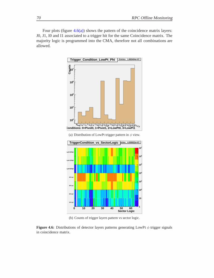
70 RPC Offline Monitoring
Four plots (figure4.6(a)) shows the pattern of the coincidence matrix layers:J0, J1, I0 and I1 associated to a trigger hit for the same Coincidence matrix. Themajority logic is programmed into the CMA, therefore not allcombinations areallowed.
Trigger Conditions: 0=Pivot0, 1=Pivot1, 2=LowPt0, 3=LowPt1None
L=0 L=1 L=0,1L=2 L=0,2L=1,2
L=0,1,2L=3 L=0,3
L=1,3L=0,1,3
L=2,3L=0,2,3
L=1,2,3L=0,1,2,3
Cou
nts
310
410
510
610
710
Trigger_Condition_LowPt_Phi Entries 1.865404e+07Trigger_Condition_LowPt_Phi
(a) Distribution of LowPt trigger pattern inφ view.
1
10
210
310
410
510
610
710
Sector Logic0 10 20 30 40 50 60
1/4 Lpt
2/4 Lpt
3/4 Lpt
4/4 Lpt
Lpt+0/2Hpt
Lpt+1/2Hpt
Lpt+2/2Hpt
TriggerCondition_vs_SectorLogic Entries 4.006922e+07TriggerCondition_vs_SectorLogic
(b) Counts of trigger layers pattern vs sector logic.
Figure 4.6: Distributions of detector layers patterns generating LowPt φ trigger signalsin coincidence matrix.

4.3.2 Detector plots 71
CM + Pad*8 + SL*56
500 1000 1500 2000 2500 3000 3500No Hits
L=0
L=1
L=0,1
L=2
L=0,2
L=1,2
L=0,1,2
L=3
L=0,3
L=1,3
L=0,1,3
L=2,3
L=0,2,3
L=1,2,3
L=0,1,2,3
No Hits
L=0
L=1
L=0,1
L=2
L=0,2
L=1,2
L=0,1,2
L=3
L=0,3
L=1,3
L=0,1,3
L=2,3
L=0,2,3
L=1,2,3
L=0,1,2,3
1
10
210
310
410
510
Figure 4.7: Distribution of trigger conditions for each single ATLAS RPC CoincidenceMatrix (CM).
The 2D plot of Figure4.6(b)is similar to the previous ones. It shows for eachSector Logic which detector layer patterns generate the trigger in phi view. Theplot is divided in two parts along the Y axis, the lower part isrelated to the LowPttrigger coincidence and the upper part to the HighPt triggercoincidence. LowPtand HighPt triggers are realized with four and two independent RPC active layersrespectively. In standard configuration LowPt trigger logic consists of 3 out of4 layers in the same trigger time window (25 nsec maximum) andHighPt triggerlogic of 1 out of 2 layers, in addition to a LowPt trigger. Consequently, not allowedlayers pattern giving trigger (such as 2 out of 4 layers in LowPt trigger) is evidenceof some inefficiency in the readout or fake triggers. The are also 2D plot similar tothe previous one but the trigger condition is monitored for each single CoincidenceMatrix (figure4.7). On the X axis is listed the coincidence matrix number shiftedby eight times the pad number and 56 times the sector logic number and on theY axis is listed all possible layer combinations that could or could not provide atrigger hits.
4.3.2 Detector plots
A further step in the RPC monitoring is the check of the quantities related tophysical detector elements (strips, panels, gas volume, etc.) instead of the elec-tronic readout channels. Clearly, this monitoring algorithm is run on data decoded

72 RPC Offline Monitoring
by using map relating the electronic channels with the detector elements. In thefollowing, the histograms produced are classified by categories shown in sec.4.2.
Chamber plots
Figures4.8 and4.9 show the most relevant histograms with 1 strip granularity(with the exception of the plot d)) and related to a single station, layer and view(with the exception of theη-φ correlation plot). To reduce the total number of his-tograms, the eta view panels of different doubletz and phi view panel of differentdoublet phi are plotted on the same histograms with increasing number of strips.Due to the large number of RPC chamber types the total number of strips in bothviews are in general different.
Together with RPC hits it is important to monitor the RPC clusters, which aredefined as a group of adjacent strips inside a window time coincidence and directlyrelated to a charged track crossing the active volume. The plot of Figure4.8(a)shows the strip profile but a similar plot exist for the baricenter of RPC clusters.An example of scatter plots between the hit arrival time and strip is given in Fig-ure4.8(b). From these plots is possible to extract time distribution to monitor the
<--- IP Rpc Eta strip EC --->0 10 20 30 40 50 60
Cou
nts/
Str
ip
0
20
40
60
80
100
120
BML3A07_Pivot0_dblPhi1_Eta_strip Entries 4564BML3A07_Pivot0_dblPhi1_Eta_strip
(a) RPC strip profile.
-110
1
10
Rpc strip0 10 20 30 40 50 60
Tim
e[ns
]
0
20
40
60
80
100
120
140
160
180
200
BML3A07_Pivot0_dblPhi1_Eta_stripvstime Entries 4564BML3A07_Pivot0_dblPhi1_Eta_stripvstime
(b) RPC time vs strip.
Figure 4.8: Example of RPC single station commissioning plots in‘RPC/Chambers/BML3A07’ folder.
RPC time alignment and spread. In Figure4.9(a)is reported a two dimensionalplot displaying the hit multiplicity of the cluster to whichthe strip belong to andin Figure4.9(b)the distribution of the cluster multiplicity for one readout panel.
Correlation plots between the two view of the same gas volumeare impor-tant because they give localized information and can removephi ‘wired-or’ and‘logical-or’ ambiguities in phi view by using the orthogonal eta view. An example

4.3.2 Detector plots 73
-110
1
10
<--- IP Rpc Eta strip EC --->0 10 20 30 40 50 60
Clu
ster
Siz
e
0
1
2
3
4
5
6
7
8
9
BML3A07_Pivot0_dblPhi1_Eta_clustersize Entries 4564BML3A07_Pivot0_dblPhi1_Eta_clustersize
(a) RPC cluster size vs strip.
Pivot0_dblPhi1_dblZ1_Eta0 1 2 3 4 5 6 7 8 9
Clu
ster
Siz
e
0
0.2
0.4
0.6
0.8
1
1.2
310×BML3A07_Pivot0_dblPhi1_dblZ1_Eta_CSdistribution Entries 1717BML3A07_Pivot0_dblPhi1_dblZ1_Eta_CSdistribution
(b) RPC cluster size distribution for onereadout panel.
-110
1
10
<--- IP Rpc Eta strip EC --->0 10 20 30 40 50 60
<---
HV
sid
e
Rpc
Phi
str
ip
RO
sid
e --
->
0
20
40
60
80
100
120
BML3A07_Pivot0_PhivsEta Entries 135185BML3A07_Pivot0_PhivsEta
(c) RPC phi view strip vs eta view strip forthe same gas volume.
1
10
210
<--- DBL_PHI0 Rpc Phi strip DBL_PHI1 --->0 20 40 60 80 100 120
<---
DB
L_P
HI0
Rpc
Phi
str
ip
DB
L_P
HI1
---
>
0
20
40
60
80
100
120
BML3A07_Pivot_dblZ1_Phi2vsPhi1 Entries 83076BML3A07_Pivot_dblZ1_Phi2vsPhi1
(d) Same view RPC strip correlation be-tween adjacent layers.
Figure 4.9: Example of RPC single station commissioning plots in‘RPC/Chambers/BML3A07’ folder.
is given in the plot of Figure4.9(c)where at a glance is possible to see the RPCcoverage. Phi-Phi or Eta-Eta strip spatial correlation between gas volumes dou-blets belonging to adjacent layer (same plane). For triggerhits the correlation isdone with respect to the innermost pivot layer. An example isgiven in the plot ofFigure4.9(d). These plots are meant to debug the RPC hardware mapping duringthe commissioning phase or after hardware intervention on the RPC chambers.

74 RPC Offline Monitoring
Sector and ATLAS plots
A similar set of plots is also produced grouping together chambers of the samesectors to still have a detailed view but more focused on global behaviour. Ex-ample of sector plots are given in The‘RPC/Sectors’ folder contains plotsshowing theη andφ view spatial correlation of RPC hits and clusters belongingto the same gas volume (see Figure4.10a).One histogram shows one RPC layer of a geometrical sector with all stations alongZ and both doubletPhi. For trigger layers the plots correspond to trigger coinci-dence in Eta and Phi views in the readout strips.
1
10
210
310
410
510
610
<--- SIDE C Rpc Eta strip SIDE A --->-200 -100 0 100 200
<---
HV
sid
e
Rpc
Phi
str
ip
RO
sid
e --
->
0
20
40
60
80
100
120
Sector07Pivot0_PhivsEta Entries 1.287338e+07Sector07Pivot0_PhivsEta
(a) One sector RPC hits map in phi view-etaview plane for one layer.
1
10
210
310
410
<--- SIDE C Rpc Eta stripSIDE A --->-400 -300 -200 -100 0 100 200 300 400
Rpc
Phi
str
ip
0
0.2
0.4
0.6
0.8
1
1.2
1.4
1.6
310×
AtlasPivot0 Entries 1472274AtlasPivot0
(b) RPC hits map in phi view-eta viewplane for one layer.
Figure 4.10: Examples of RPC sector (a) and RPC atlas (b) plots.
RPC overview plots
Overview plots monitor integrated quantities for the entire ATLAS detector (seeFigure4.11).The plots Figure4.11(a)and 4.11(b)shows the distribution of the number ofRPC hits and the number of RPCη andφ clusters per event, and the plot of Fig-ure4.11(c)shows the time distribution of all RPC hits for one view. No clean-upcuts are used to fill the timing plots which have a range of 200 nsec (equal to read-out window of RPC level-1 trigger system) with a total numberof 64 bins (binsize equal to 3.125 nsec to the RPC internal clock). The plotsof Figure4.11(d)shows the cluster size distribution of readout strips for one view.
Several two dimensional histograms map the RPC detector status in a con-venient way. Two example of these histograms are given in Figure 4.12(a)and

4.3.2 Detector plots 75
[counts]0 20 40 60 80 100 120 140
Num
ber
of H
its/E
vent
s
0
100
200
300
400
500
600
700
800
900
Number_of_RPC_hits_per_event Entries 59999Mean 81.8RMS 25.48
Number_of_RPC_hits_per_event
(a) Distribution of RPC hits per event.
[counts]0 20 40 60 80 100 120 140
Num
ber
of C
lust
ers/
Eve
nts
0
0.2
0.4
0.6
0.8
1
1.2
1.4
1.6
310×Number_of_RPC_clusters_per_event Entries 59999
Mean 57.49RMS 16.69
Number_of_RPC_clusters_per_event
(b) Distribution of RPC clusters perevent.
Time Phi View [ns]0 20 40 60 80 100 120 140 160 180 200
Cou
nts/
(3.1
25ns
)
20
30
40
50
60
310×Phi_Time_Distribution Entries 2433168
Mean 84.45RMS 49.19
Phi_Time_Distribution
(c) Time distribution of RPC hits in phiview.
Cluster Size Phi view0 1 2 3 4 5 6 7 8 9
Cou
nts
0
0.2
0.4
0.6
0.8
1
1.2
1.4610×
Phi_ClusterSize_Distribution Entries 1913053Mean 1.478RMS 1.006
Phi_ClusterSize_Distribution
(d) Cluster size distribution of RPC hitclusters in phi view.
Figure 4.11: Examples of RPC overview plots in ‘RPC/Overview’ folder. Data are fromphysics-RPCwBeam stream.
4.12(b). The first one shows the RPC trigger hits map. The same kind of mapexists for RPC hits for each detector layer. The RPC map have Eta station numberalong the X axis and the sector number un-folded in three planes along Y (seedashed lines).The second one shows the map of correlated Phi and Eta hits of the entire ATLASRPC detector for the corresponding layer.Each bin in both axis corresponds to two crossing orthogonalstrips of the samegas volume and is filled if both strips are found in the event. One histogram showsall 16 RPC geometrical sectors of one layer un-folded in Phi view. The rangealong the Y axis (Phi view) is equal to the number of phi strip for that layer. The

76 RPC Offline Monitoring
positive (negative) range and along the X axis (Eta view) is equal to the maximumnumber of eta strip for that layer and side A (C) Eta strips of side A (C) are plot-ted positive (negative). There are also histograms similarto the previous ones, butwith spatial coordinates Phi and Z in mm are used instead of strip number.
<--- SIDE C Rpc Eta strip SIDE A --->
-400 -300 -200 -100 0 100 200 300 400
Rpc
Phi
str
ip
0
200
400
600
800
1000
1200
1400
1600
1
10
210
310
410
510
610
(a) Low Pt trigger hits map.
<--- SIDE C Rpc Eta stripSIDE A --->
-400 -300 -200 -100 0 100 200 300 400
Rpc
Phi
str
ip
0
200
400
600
800
1000
1200
1400
1600
1
10
210
310
410
510
(b) Pivot 0 plane hits map.
Figure 4.12: .

4.3.2 Detector plots 77
Trigger data
Histograms intended to monitor the setting and the responseof the trigger to theprogrammed spatial coincidence are also produced by RPC off-line monitoring.The width of the spatial geometrical coincidence (named ‘trigger road’) can beprogrammed to correspond up to 3+3 high transverse momentumtrack values.
Figure4.13(a)shows the distribution of the conventional number named ‘Thresh-old’ which labels the trigger configuration for one view. Other six histogramsshows the scatter plot between the ‘Threshold’ and the 2D impact parameter ofthe trigger segment defined by trigger hits and the confirm hits. Figure4.13(b)clearly shows a projective trigger road in non-bending viewas extracted fromcosmics data. At the time of this writing the trigger road histogram granularityis only limited to small and large sectors, in addition to Low-HighPt and Phi-Etaview.
LPt1: 0 LPt2: 2 LPt3: 3 HPt1: 0 HPt2: 2 HPt3: 3 NC:990
0.2
0.4
0.6
0.8
1
610×RPC_Threshold_Phi Entries 11
Mean 1.631RMS 1.421
RPC_Threshold_Phi
(a) Distribution of RPC trigger hit thresholdin phi view.
1
10
210
310
410
510
-1 -0.8 -0.6 -0.4 -0.2 0 0.2 0.4 0.6 0.8 1
LPt1: 0
LPt2: 2
LPt3: 3
HPt1: 0
HPt2: 2
HPt3: 3
NC:99
RPC_TriggerRoad_Large_Phi Entries 600RPC_TriggerRoad_Large_Phi
(b) RPC trigger segment impact parameterin the corresponding view.
Figure 4.13: Examples of RPC trigger road plots in ‘RPC/TriggerRoad’. Data are fromphysics-MuonswBeam stream and run 148209 (1,850,000 events analysed).
Luminosity blocks
The ATLAS data is divided in luminosity blocks (‘LumiBlocks’), which shouldcorrespond to the minimum time interval where the instantaneous luminosity shouldbe evaluated. In order to monitor the instantaneous luminosity by the RPC detec-tor a chain of histograms storing information for each groupof contiguous eventswere implemented.

78 RPC Offline Monitoring
For every luminosity block XXX these specific histograms arebooked andfilled by the monitoring algorithm and tagged as ‘luminosityblock histograms’.Because the off-line monitoring at Tier-0 is split in data-files and sub-jobs, usuallya data-file don’t correspond to a luminosity block. The luminosity block histogrammerging is done at Tier-0 with an appropriate tool called (‘mergeLBintervals’).
The RPC luminosity block histograms are filled with the corresponding triggerhits. These plots are intended to monitor the RPC trigger rate from the readouthits with time granularity equal to the run luminosity block.
4.4 RPC and MDT correlation monitoring
The ‘MdtVsRpcRawDataValAlg’ package was developed to check spatialcorrelation and time synchronization between raw hits provided by MDT and RPCdetectors. This was done by comparing the longitudinal position of MDT tubehits and RPC Eta strip hits belonging to the same station and plane. In order tosuppress a residual MDT noise a cut on the MDT ADC of about 50 counts isalways implied
Entries 13577
Mean 731.2
RMS 255
Time Spectrum [ns]
0 200 400 600 800 1000 1200 1400 1600 1800 2000
Cou
nts
0
100
200
300
400
500 Entries 13577
Mean 731.2
RMS 255
(a) MDT TDC spectra for tracks crossingHV or RO side.
1
10
210
<--- IP Rpc Eta strip EC --->0 5 10 15 20 25 30 35 40
<---
IP
Mdt
wire
num
ber
AD
C C
ut O
N E
C -
-->
0
5
10
15
20
25
30
35
40
BML5A05_Pivot_MDTtube_vs_RPCstrip Entries 38341BML5A05_Pivot_MDTtube_vs_RPCstrip
(b) MDT tube vs RPC eta strip of one planeinside a station.
Figure 4.14: Examples of single station commissioning plots correlating RPC and MDT.from ‘MDTvsRPC/Chambers/BML5A05’ folder. The noise cut onMDT ADC of 50counts is implied. The data are from physics-RPCwBeam stream.
The correlations is done between RPC strip number and MDT tube layer num-ber. Because a MDT tube is long as the entire (inφ direction) chamber width andit is coupled to two RPC panels, the RPC doublet readout strippanel index allowsto establish the side of the tube when the hit was generated bythe crossing track.

4.5 RPC track monitoring 79
This is important in order to monitor asymmetry in MDT detector response alongthe tube. Figure4.14(a)shows a histograms displaying the MDT TDC spectra innsec of MDT tube hits correlated to the corresponding RPC doublet.
Two dimensional plots showing the z hits correlation of one plane betweenRPC and MDT for the entire sector (see Figure4.14(b)are important in order toverify the muon system synchronization with a limited number of histograms. Onthe X axis the RPC Eta strip Z coordinate in mm is plotted, whereas on the Y axisthe MDT tube center Z coordinate in mm is plotted. The axis ranges are generatedautomatically according to the minimum and maximum Z coordinate of RPC andMDT tube for the plane and sector.
4.5 RPC track monitoring
Because RPCs can measure eitherη andφ coordinates of crossing muons, a track-ing algorithm that use only RPC data has been implemented in off-line monitoring[40]. It is capable of producing a fast feedback on RPC detector data quality, with-out using informations from MDT precision chambers and without relying on thefull ATLAS event reconstruction and combined quantities.
The RPC tracking is based on RPC space points, which are defined by orthog-onal RPC baricenters of cluster of the same gas volume. The pattern recognitionis seeded by a straight line, which is defined by two RPC space points belonging,respectively, to low-Pt and pivot planes of the same or nearby station. RPC spacepoints not part of any previous tracks and inside a predefineddistance (50 mm)from the straight line are associated to the pattern. Resulting patterns with pointsin at least 3 out of 4 layers in low-pt and pivot planes are retained and a leastsquare linear fit is performed in two orthogonal views.
The patter recognition parameters can be selected by joboptions. The ‘Merge-PointDistance’, with a default value of 50 mm, establishes when a space point canbe merged in a seeded RPC track. The ‘EtaStationSpan’, with adefault value of 2,and the ‘DoublePhiSpan’, with a default value of 1, establish the range of stationsalong z and sectors along phi that a track can cross in order toavoid pathologicaltracks. With the default values a cosmic track crossing the detector top to bottomresults in two RPC tracks.
From data triggered with cosmics about 95 % percent of eventshave at leastone RPC track; this is due to the strong correlation between the pattern recognitionand the trigger algorithm. Applying a quality cut of chi2/dof < 1 about 70 % ofevents have at least a good tracks and 10 % with more than one. This quality trackcut can be set by joboption changing the parameter ‘Chi2dofCut’.

80 RPC Offline Monitoring
LowPt track
HighPt track
RPC 3D space point
Phi strip
Eta strip
a)
b)
Figure 4.15: Schematic view of the RPC standalone tracking algorithm. Starting frometa and phi clusters (with size less than 4), RPC 3-D space points are build (b). Fromthese points, a pattern recognition with linear fit is performed requiring at least 3 hits over4 RPC layers in Low Pt stations and at least 1 hits over 2 layersin Highpt stations (a).
Detection efficiency
The detection efficiency is measured by repeating 6 times theRPC tracking. Ateach iteration the layer under test is removed from the pattern recognition andtrack fitting. The track reconstructed is then extrapolatedto the active gas volumeof the removed layer and the crossing point evaluated. No error analysis on theextrapolation accuracy is done at the moment of writing. Theefficiency is evalu-ated only if the crossing point is inside a fiducial region expressed in term of stripdistance from active volume boundaries. The fiducial bordersize can be set by thejoboptions parameter ‘nstripfiducial’ which by default is zero. If the extrapolationpoint is inside the fiducial region then the gas volume is assumed to be efficient ifat least one hit is found inside a search window expressed in terms of strips by the

4.5 RPC track monitoring 81
joboption parameter ‘nstripfiduceff’, which have a defaultparameter of 3 strips.An unbiased measurement of the RPC efficiency is also made if the detector
is part of the trigger decision. In fact, the 3 out of 4 majority trigger logic makesthe layer under test response irrelevant in the trigger decision when the other threelayers have a good track.
Hit on track
Uncorrelated noise hit
Correlated noise hit
Figure 4.16: Definition ofon trackshits,correlatedanduncorrelatednoise hits. Hits notassociated to any track are classified as “noise” of RPC chambers: hits belonging to twodifferent gas gap of the same RPC doublets are defined “correlated noise”, whereas hitspresent in only one gas volume are define “uncorrelated noise”.
Noise Measurements
The detector total noise is measured taking into account RPChits not belongingto any RPC track, that is, farther away than the parameter ‘MergePointDistance’.The correlated noise is defined by RPC noise hits belonging tothe same chamberbut different gas volume and inside a spatial window defined by the parameter“mergePointDistance”. The parameters occurring in the noise definitionare kept equal to the track pattern recognition parameters to stay conservative.This could change if further needs emerge.
The noise is expressed in term of Hertz per centimeter squareby the formula:
Noise =Counts
Events · w · surface,
wherew is the rpc readout time window and is equal to 0.2µsec, the maximumvalue allowed by the hardware and used for cosmics.

82 RPC Offline Monitoring
Cosmics run versus collisions run
Cosmic rays arrive randomly in time and not uniformly on detector surface. Thismakes detector studies with cosmics less accurate then withbeam collisions.Tracks produced by beam collisions are synchronous with beam clock, pointingto the interaction point, and uniform in azimuthal angle andpseudo-rapidity. Thedifficultly with beam is due to the presence of the magnetic field and operationat high luminosity. The above described pattern recognition and the track qualitycut correspond, in magnetic field, to a cut in transverse momentum. At high lumi-nosity a large uncorrelated and correlated background could increase the numberof fake tracks significantly. Studies with a Monte Carlo sample with pile-up andcavern background are underway at the time of this writing.
Commissioning histograms are related to single chamber andhave 1 stripgranularity. The plot of figure4.17(a)shows the profile of strip crossed by thetracks reconstructed with the other layers. Similar histograms are filled with theprofile of strips crossed by the tracks, reconstructed with the other layers, witha nearby fired strip in the same view (figure4.17(b)) and in both views (figure4.17(c), respectively. The three previous histograms allow to compute the readoutpanel detection efficiency not conditionated or conditionated to the other measur-ing view. The histogram of Figure4.17(d)show the distribution of the spatialresidual defined as the difference between the projected track local coordinate andthe RPC cluster local coordinate. The track extrapolation errors are not subtractedfrom the residual evaluation.
RPC tracks overview plots
The general plots show quantities related to RPC track standalone capability forthe entire ATLAS detector. In this section only some of the overview plots aredescribed (see Figure4.18) and the other general plots are discussed in Section5.2.1where shifter plots are described.
The quality of the RPC tracks reconstructed with all layers are monitored bythe distribution of the chi2 per degrees of freedom, the 3D RPC space points mul-tiplicity and spatial and time residual. The histogram of Figure4.18(a)display thedistribution of the total chi2 per degree of freedom (both views) and the histogramof Figure4.18(b)shows the scatter plot between the chi2 per degree of freedomofthe two views separately. The distribution of the number of 3D RPC space pointsassociated to the track and used by the straight line fit is plotted on the histogramof Figure4.18(e). In addition, the RPC tracks are classified according to the 3DRPC points layer combination and the distribution is shown by the histogram ti-tled of Figure4.18(f). Spatial track residual distribution and the time spread ofthe 3D RPC space point are also reported in Figure4.18(c)and 4.18(d).

4.5 RPC track monitoring 83
<-HV side Rpc Phi strip RO side->
0 20 40 60 80 100 120
co
un
t/str
ip
10
20
30
40
50
60
70
(a) Strip profile of RPC tracks projected on theremoved readout panel.
<-HV side Rpc Phi strip RO side->
0 20 40 60 80 100 120
co
un
ts / s
trip
10
20
30
40
50
60
70
(b) Strip profile of RPC tracks projected on theremoved readout panel and matching RPC clus-ter hits.
<-HV side Rpc Phi strip RO side ->
0 20 40 60 80 100 120
co
un
ts / s
trip
10
20
30
40
50
60
70
(c) Strip profile of RPC tracks projected on theremoved readout panel and matching RPC clus-ter hits in both views.
Mean -0.9552
RMS 12.73
Residual [mm]
-100 -50 0 50 100
Co
un
ts /
mm
0
50
100
150
200
250
300
350 Mean -0.9552
RMS 12.73
(d) Spatial residual distribution of a strip readoutpanel.
Figure 4.17: Examples of RPC single station commissioning plots.
In order to visualize directly the origin of the tracks (cosmic, random, singlebeam, beam collisions, ...) and the trigger stream (RPC, TGC, Lucid, MTBS, ...)the reconstructed tracks are extrapolated on different planes such as (x,z) plane aty = 81 m, corresponding to the ATLAS surface (see Figure5.6(f)). In addition,two-dimensional track parameters distribution in term of track pseudo-rapidityvariableη = −ln(tan(θ/2), with θ the track poloidal angle, track impact pa-rameter b and the track azimuthal angleφ are also produced (Figures4.19(a)and4.19(b)). Finally, one dimensional track parameters distributionare shown for allabove quantities (see Figures4.19(c), 4.19(d)and4.19(e)).
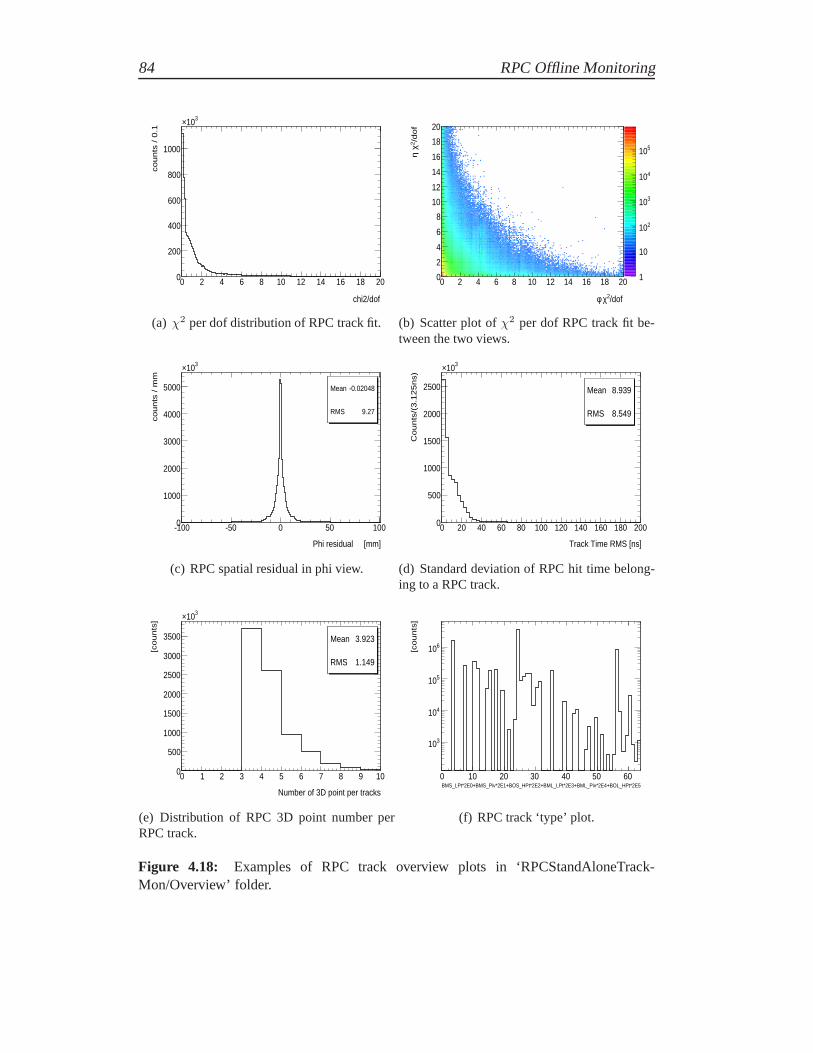
84 RPC Offline Monitoring
chi2/dof
0 2 4 6 8 10 12 14 16 18 20
co
un
ts / 0
.1
0
200
400
600
800
1000
310×
(a) χ2 per dof distribution of RPC track fit.
/dof2χ φ
0 2 4 6 8 10 12 14 16 18 20
/do
f2 χ
η
0
2
4
6
8
10
12
14
16
18
20
1
10
210
310
410
510
(b) Scatter plot ofχ2 per dof RPC track fit be-tween the two views.
Mean -0.02048
RMS 9.27
Phi residual [mm]
-100 -50 0 50 100
co
un
ts / m
m
0
1000
2000
3000
4000
5000
310×
Mean -0.02048
RMS 9.27
(c) RPC spatial residual in phi view.
Mean 8.939
RMS 8.549
Track Time RMS [ns]
0 20 40 60 80 100 120 140 160 180 200
Co
un
ts/(
3.1
25
ns)
0
500
1000
1500
2000
2500
310×
Mean 8.939
RMS 8.549
(d) Standard deviation of RPC hit time belong-ing to a RPC track.
Mean 3.923
RMS 1.149
Number of 3D point per tracks
0 1 2 3 4 5 6 7 8 9 10
[co
un
ts]
0
500
1000
1500
2000
2500
3000
3500
310×
Mean 3.923
RMS 1.149
(e) Distribution of RPC 3D point number perRPC track.
BMS_LPt*2E0+BMS_Piv*2E1+BOS_HPt*2E2+BML_LPt*2E3+BML_Piv*2E4+BOL_HPt*2E50 10 20 30 40 50 60
[co
un
ts]
310
410
510
610
(f) RPC track ‘type’ plot.
Figure 4.18: Examples of RPC track overview plots in ‘RPCStandAloneTrack-Mon/Overview’ folder.

4.5 RPC track monitoring 85
pseudo-rapidity
-1.5 -1 -0.5 0 0.5 1 1.5
ph
i a
ng
le [d
eg
]
0
20
40
60
80
100
120
140
160
180
1
10
210
310
(a) Scatter plot of pseudo-rapidityη vs azimutalangleφ of reconstructed tracks.
rpc track pseudo-rapidity
-1.5 -1 -0.5 0 0.5 1 1.5
rpc tra
ck d
ista
nce
fro
m IP
[m
m]
0
2000
4000
6000
8000
10000
12000
1
10
210
(b) Scatter plot of impact parameter b vs azimu-tal angleφ of reconstructed tracks.
Mean 0.04847
RMS 0.3525
pseudo-rapidity
-1.5 -1 -0.5 0 0.5 1 1.5
Co
un
ts
0
10000
20000
30000
40000
50000
60000
70000 Mean 0.04847
RMS 0.3525
(c) Distribution of pseudo-rapidityη parameterof reconstructed tracks.
Mean 90.27
RMS 25.18
phi angle [deg]
0 20 40 60 80 100 120 140 160 180
Co
un
ts
0
20
40
60
80
100
120
140
160
180
310×
Mean 90.27
RMS 25.18
(d) Distribution of azimutal angleφ parameterof reconstructed tracks.
Mean 5538
RMS 2402
rpc track distance from IP [mm]
0 5000 10000 15000 20000
co
un
ts/(
50
mm
)
0
2000
4000
6000
8000
10000
12000
14000
Mean 5538
RMS 2402
(e) Distribution of impact parameter b of recon-structed tracks.
Figure 4.19: Examples of track parameters scatter and distribution plots.

86 RPC Offline Monitoring

5RPC Data Quality
The applications of RPC offline monitoring consist of:
• giving informations about the status and the behaviour of the detector almostin real-time, spotting possible problems which can occurs during detectoroperation;
• defining the quality of data recorded and therefore the possibility to be usedfor analysis;
• defining the effective detector working parameter (such as efficiency, clustersize, etc.), which must be used to obtain Monte Carlo simulation as realisticas possible.
In this chapter, the second and the third items will be detailed, whereas theresults of the application of monitoring package to study detector performanceare postponed to next chapter.
5.1 Muon Spectrometer Data Quality Chain
Data quality is a crucial issue for physics analysis. The data quality process hasbeen introduced with the aim of marking reconstructed data of every run as usableor not for performance and physics analysis in ATLAS experiment. Because thesize of the ATLAS collaboration and the complexity of the detector, it is necessaryto use a tool that allows final users to extract good runs. Thistool is designed tohide technical detector details to final users.
The quality information of detectors is summarized in “traffic lights”-like flags[41], that can assume five values described in table5.1. Data quality flags aregenerated for each sub-detectors and for each data quality source (detector con-trol system, on-line and off-line) and have the time granularity of one luminosityblock. All informations are stored in a dedicated conditions database: in total,there are more than 100 data quality flags recorded. As a result, by analysing thedata quality flags obtained above, officialgood run lists(distinct for individual
87

88 RPC Data Quality
Status Light Description
Disabled black indicates that the system has been disabled.Undefined gray indicates that a clear statement cannot be made (for
example in case of short runs with a few statistics orin case or data quality problems).
Bad red indicates that the fraction of data is considered notsuitable for physics analysis.
Good green indicates that the fraction of data is considered suit-able for physics analysis.
Flawed yellow indicates that data are not good, but are possible re-coverable. The flag isyellow if a calibration work orthe precise status determination is still underway, andthe use of the data should be postponed until the workhas been finalized (in the chosen model, after the finalreprocessing the detector status should be onlygoodor bad).
Table 5.1: Data quality status flag codification.
physics objects) are defined and delivered to physics group for physics analysisand publication of physics results.
Data monitoring is first done online, on a sampled subset of the events be-ing recorded, to quickly spot problems and instabilities. We focus here on offlinemonitoring, which is performed after the data has been taken, ideally in parallel tothe event reconstruction chain (see Figure5.1), at the CERN computer farmTier-0(see section4.1.2). Muon offline monitoring ensures that the initial data is satis-factory (first pass) or that the calibrations are valid (second and higher passes).The off-line data quality process of ATLAS is based primarily on analysing his-tograms produced by monitoring tool that runs in Athena (seechapter4). Thesetools are active during prompt reconstruction but can also be used independently.Tools are already implemented to monitor information ranging from hardwarereadout errors to dimuon masses for J/ψ and Z reconstruction.
There are two ways by which the histograms are analysed:
manual checks: histograms are viewed by shifters, both in ATLAS control roomduring data taking and off-line after run end;
automatic checks: the automatic tool DQMF (Data Quality Monitoring Frame-work) [42] performs checks of histograms by applying specific methods(detailed below) and publish the resulting flags on web pages.

5.2 RPC Data Quality 89
Figure 5.1: Schematic diagram of the flow of the offline muon Data Quality Monitoringwith respect to the data processing.
The monitoring algorithms can only use a limited amount of memory (typi-cally no more than 100 MB per algorithm) and time (less than a second per event);this is particularly important for central processing of raw data at CERN, so thatmonitoring histograms are created as soon as the data itselfis available.
5.2 RPC Data Quality
Data quality plots are automatically presented in a dedicated web page1, figure5.2shows links to different technologies plots, in particularlinks to folders in whichRPC histograms are grouped are expanded; plots which are mainly meant to bechecked by human shifters are detailed in paragraph5.2.1, whereas automaticchecks of histograms are shown in paragraph5.2.3.
5.2.1 RPC Shifter plots
In this section the subset of histograms produced by monitoring package andchecked by data quality shifter is presented. Shifter plotsgive the general sta-tus of the detector at one glance, without knowing RPC detector details.
RPC plots
The two-dimensional plot Figure5.3(a) shows the geometrical map ofη vs φview trigger hits of RPC in the spectrometer. The chosen coordinates are the
1https://atlasdqm.cern.ch/webdisplay/tier0/

90 RPC Data Quality
Figure 5.2: Links on the ATLAS off-line data quality web display (RPC folders areexpanded).
pseudo-rapidity and the azimuthal angle. It is intended to show the RPC triggergeometrical coverage.
There are other two-dimensional plots showing the total counts of RPC inLowPt and HighPt stations, without distinguish betweenη andφ view hits. It isintended to show the RPC trigger layout coverage. The two-dimensional plot ofFigure5.3(b)shows the total counts of RPC without distinguish betweenη andφview hits. On thex axis there is theη station number within a geometrical sector.On they axis there are shown the total counts of LowPt, Pivot, and HighPt planesfor all geometrical sectors.

5.2.1 RPC Shifter plots 91
Eta
-1 -0.5 0 0.5 1
Phi
(r
ad)
-3
-2
-1
0
1
2
3
1
10
210
310
410
510
610
(a) RPC LowPt trigger hit map in (phi,eta) plane.
<--- SIDE C Rpc Eta Station SIDE A --->
-6 -4 -2 0 2 4 6
Rpc
Sec
tor
+ 1
6 *
(LP
t=0,
Piv
=1,
HP
t=2)
0
5
10
15
20
25
30
35
40
45
1
10
210
310
410
510
610
(b) RPC hit chamber map.
Figure 5.3: Examples of RPC general status plots in ‘RPC/GLOBAL’ folder(data arecosmics muons taken during November 2009 ).
RPC level 1 plots
Regarding to monitoring of RPC triggers (see section4.3.1), the plot of Fig-ure5.4(a)shows the combination of LowPt RPC layers inside a coincidence ma-trix in correspondence to a trigger hit in the readout for each RPC Sector Logic.On they axis, the LowPt and HighPt trigger combinations are shown separately,the first one at the bottom part of the plot and the second one inthe upper part.
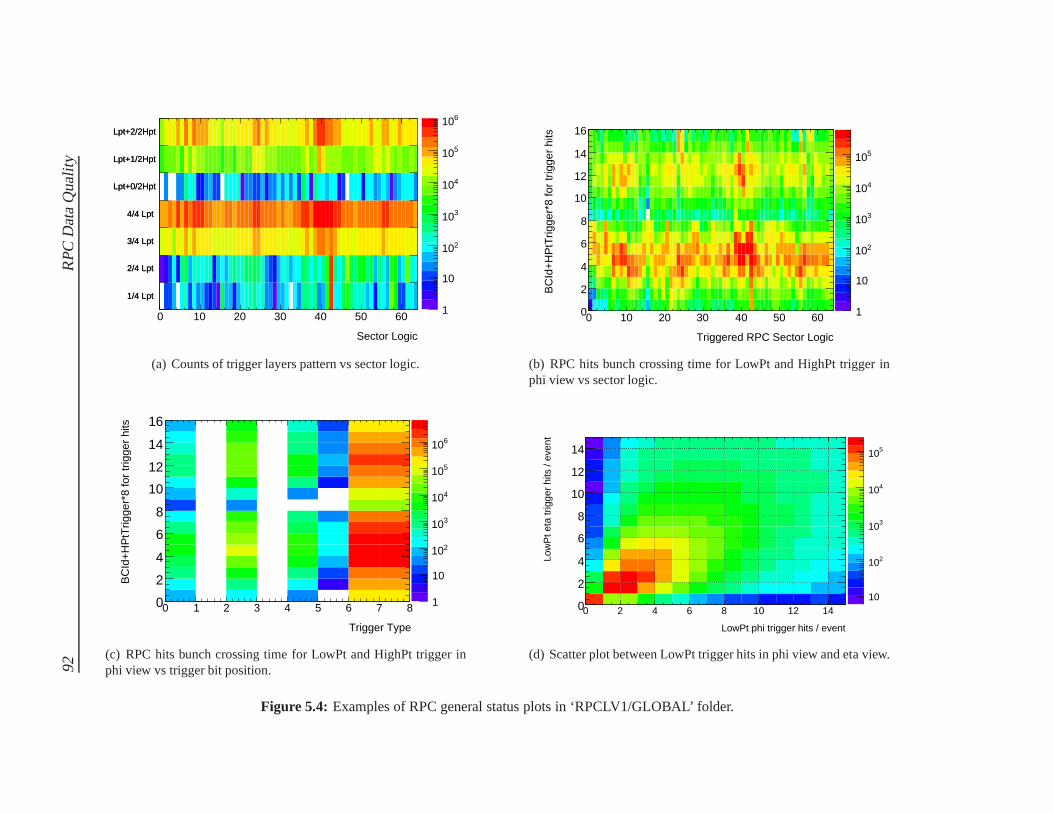
92R
PC
Dat
aQ
ualit
y
Sector Logic
0 10 20 30 40 50 60
1/4 Lpt
2/4 Lpt
3/4 Lpt
4/4 Lpt
Lpt+0/2Hpt
Lpt+1/2Hpt
Lpt+2/2Hpt
1/4 Lpt
2/4 Lpt
3/4 Lpt
4/4 Lpt
Lpt+0/2Hpt
Lpt+1/2Hpt
Lpt+2/2Hpt
1
10
210
310
410
510
610
(a) Counts of trigger layers pattern vs sector logic.
Triggered RPC Sector Logic
0 10 20 30 40 50 60
BC
Id+
HP
tTrig
ger*
8 fo
r tr
igge
r hi
ts
0
2
4
6
8
10
12
14
16
1
10
210
310
410
510
(b) RPC hits bunch crossing time for LowPt and HighPt triggerinphi view vs sector logic.
Trigger Type
0 1 2 3 4 5 6 7 8
BC
Id+
HP
tTrig
ger*
8 fo
r tr
igge
r hi
ts
0
2
4
6
8
10
12
14
16
1
10
210
310
410
510
610
(c) RPC hits bunch crossing time for LowPt and HighPt triggerinphi view vs trigger bit position.
LowPt phi trigger hits / event
0 2 4 6 8 10 12 14
Low
Pt e
ta tr
igge
r hi
ts /
even
t
0
2
4
6
8
10
12
14
10
210
310
410
510
(d) Scatter plot between LowPt trigger hits in phi view and eta view.
Figure 5.4: Examples of RPC general status plots in ‘RPCLV1/GLOBAL’ folder.
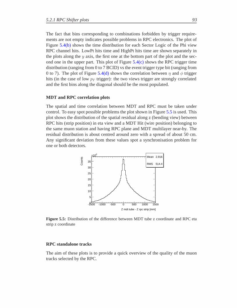
5.2.1 RPC Shifter plots 93
The fact that bins corresponding to combinations forbiddenby trigger require-ments are not empty indicates possible problems in RPC electronics. The plot ofFigure5.4(b)shows the time distribution for each Sector Logic of the Phi viewRPC channel hits. LowPt hits time and HighPt hits time are shown separately inthe plots along they axis, the first one at the bottom part of the plot and the sec-ond one in the upper part. This plot of Figure5.4(c)shows the RPC trigger timedistribution (ranging from 0 to 7 BCID) vs the event trigger type bit (ranging from0 to 7). The plot of Figure5.4(d)shows the correlation betweenη andφ triggerhits (in the case of lowpT trigger): the two views trigger are strongly correlatedand the first bins along the diagonal should be the most populated.
MDT and RPC correlation plots
The spatial and time correlation between MDT and RPC must be taken undercontrol. To easy spot possible problems the plot shown in Figure5.5is used. Thisplot shows the distribution of the spatial residual along z (bending view) betweenRPC hits (strip position) in eta view and a MDT Hit (wire position) belonging tothe same muon station and having RPC plane and MDT multilayernear-by. Theresidual distribution is about centred around zero with a spread of about 50 cm.Any significant deviation from these values spot a synchronisation problem forone or both detectors.
Mean 2.916
RMS 514.4
Z mdt tube - Z rpc strip [mm]
-1500 -1000 -500 0 500 1000 1500
Cou
nts
0
5
10
15
20
25
30
35
610× Mean 2.916
RMS 514.4
Figure 5.5: Distribution of the difference between MDT tube z coordinate and RPC etastrip z coordinate
RPC standalone tracks
The aim of these plots is to provide a quick overview of the quality of the muontracks selected by the RPC.

94 RPC Data Quality
Number of rpc tracks per event
0 1 2 3 4 5 6 7 8 9 10
[co
un
ts]
0
200
400
600
800
1000
1200
310×
(a) RPC tracks multiplicity per event.
Track Time Residual [ns]
-100 -80 -60 -40 -20 0 20 40 60 80 100
Co
un
ts/(
3.1
25
ns)
0
500
1000
1500
2000
310×
(b) RPC track hit time deviation from the aver-age.
(0=LPt0,1=LPt1,2=Piv0,3=Piv1,4=HPt0,5=HPt1)+(eta=0,1=phi)*6+(0=Small,1=Large)*12
0 2 4 6 8 10 12 14 16 18 20 22 24
Nu
mb
er
of
Tra
cks
210
220
230
240
250
260
270
280
290
300310×
(c) Number of RPC tracks projected on the re-moved layer.
LayerType(LPt0,LPt1,Piv0,Piv1,HPt0,HPt1) + ( Eta or Phi)*6 + (Small or Large)*12
0 2 4 6 8 10 12 14 16 18 20 22 24
Nu
mb
er
of
Hits
190
200
210
220
230
240
250
260
310×
(d) Number of RPC tracks projected on the re-moved layer and matching RPC cluster hits.
LayerType(LPt0,LPt1,Piv0,Piv1,HPt0,HPt1) + ( Eta or Phi)*6 + (Small or Large)*12
0 2 4 6 8 10 12 14 16 18 20 22 24
Ave
rag
e L
aye
r E
ffic
ien
cy
0.85
0.86
0.87
0.88
0.89
0.9
0.91
0.92
0.93
(e) Average layer efficiency with respect to RPCtrack coverage.
(f) Cosmic muon map reconstructed on surface( z = 81m ).
Figure 5.6: Examples of RPC track general status plots in ‘RPCStandAloneTrack-Mon/GLOBAL’ folder. Data are from physics-RPCwBeam streamand run 113860(6,600,000 events analysed).

5.2.2 Data Quality Monitoring Framework 95
The plot of figure5.6(a)shows the distribution of the number of tracks recon-structed in each event, provided by the RPC standalone reconstruction algorithm.
The plot of figure5.6(b)shows the distribution of the Root Mean Square val-ues of RPC hit times belonging to a single RPC standalone track. After RPCtiming calibration, a spread much less than one bunch crossing is expected.
The plot of figure5.6(c)and 5.6(d)shows the total number of tracks extrapo-lated on each RPC layer and the number of extrapolated trackswith a near-by hit.The RPC layers are divided in Large and Small sectors, in Eta and Phi views for atotal of 24 bins.
The plot of Figure5.6(e)is the ratio of the two previous plots and shows theefficiency.
The plot of Figure5.6(f) shows the two-dimensional distribution of impactparameters of tracks reconstructed by the code RPCStandAlone, extrapolated tothe surface. Are clearly visible the areas from which comes the greatest numberof muons reconstructed by the RPC, which correspond to the two holes of the AT-LAS experimental cavern, through which the ATLAS componentwere descendingfor installation. Besides these areas, there are two secondary areas across which anot negligible1 number of muons reaches the detector. These areas are related tothe shaft of the experimental cavern lifts.
The shifter plots above described are summarized in the table5.2according tocorresponding monitoring algorithm.
5.2.2 Data Quality Monitoring Framework
TheData Quality Monitoring Framework(DQMF) [42] is a software tool devel-oped to perform automated analysis on monitoring data and toencode results inflags as defined in table5.1.
The DQMF is based on applying some operations on histograms produced bymonitoring package: for example, the operation can be the evaluation of the meanor the RMS of a histogram, the Kolmogorov test, the counting of the number ofbins with content above or below a predefined threshold, a comparison with apredefined histogram used as reference, etc. The numerical result of these oper-ations is compared with the thresholds which define thegoodandbad interval.The operation are defined in theDQMF algorithm, that are managed by a generalconfiguration script.Figure5.7shows an example of application of DQMF to the two-dimensional plotshowing the trigger coverage of RPC in side-A of “lowpT ” stations. Each bin in
1The not negligible amount of cosmics from elevator shafts, smaller than cavern holes, wasunexpected. This “discovery” of ATLAS elevators was an unintentional application of physicsNobel prize L. W. Alvarez proposal [43] to search hidden rooms in Egyptian pyramids by lookingat cosmics flux anysotropy.

96 RPC Data Quality
RpcLv1RawDataValAlgType Title Description
TH2I TriggerCondition_vs_SectorLogic Majority trigger logic vs Sector LogicTH2I rpclv1_BCid_vs_SectorLogic Trigger Bunch Crossing vs Sector LogicTH2I rpclv1_BCid_per_TriggerType Trigger Bunch Crossing vs type of trigger
RpcRawDataValAlgType Title Description
TH2I EtavsPhi_TriggeredMuons LowPt trigger map in (φ,η) planeTH2I GlobalHitsPerRPCMiddle RPC Middle Station hit mapTH2I GlobalHitsPerRPCOuter RPC Outer Station hit mapTH2I rpc2DEtaStation RPC Station hit map
MdtVsRpcRawDataValAlgType Title Description
TH1I MdtRpcZdifference RPC and MDT residual along z
RPCStandaloneTracksMonType Title Description
TH2I rpczxSurfaceView RPC track map on surfaceTH2I rpctrack_bvseta RPC track pseudo-rapidity vs impact param-
eterTH1I rpcNtracks RPC number of tracks per eventTH1I TimeTrackResidual RPC track cluster time residualTH1I Track_Projected_on_Layer RPC projected tracks on RPC layerTH1I Hit_on_Track_Layer RPC projected tracks with corresponding
hitsTH1I Layer_Efficiency RPC layer average efficiency
Table 5.2: RPC Shifter plots with a short description.
the histogram corresponds to one RPC chamber (in the x axis there is the chamberindex and all 16 RPC sectors are unfolded in y axis) and contains the number ofRPC LowpT trigger signals. The DQMF algorithm (all operational parameters arereported in figure) used here checks (for every bin) if the bincontent is above thethreshold (the parameterBinThreshold set to 5 in this case). The total numberof bins satisfying the above condition, calledNBins, is the central parameter ofthe algorithm: it is compared with the auto-explicative thresholds of red and green
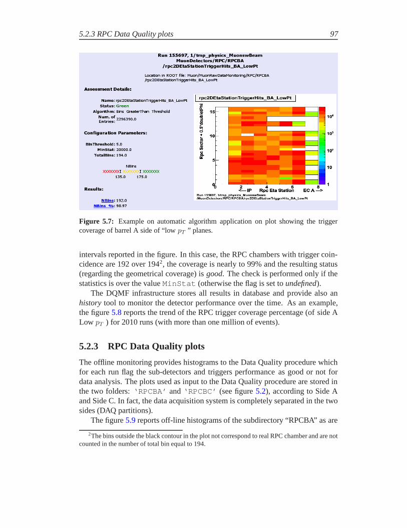
5.2.3 RPC Data Quality plots 97
Figure 5.7: Example on automatic algorithm application on plot showingthe triggercoverage of barrel A side of “lowpT ” planes.
intervals reported in the figure. In this case, the RPC chambers with trigger coin-cidence are 192 over 1942, the coverage is nearly to 99% and the resulting status(regarding the geometrical coverage) isgood. The check is performed only if thestatistics is over the valueMinStat (otherwise the flag is set toundefined).
The DQMF infrastructure stores all results in database and provide also anhistory tool to monitor the detector performance over the time. As anexample,the figure5.8reports the trend of the RPC trigger coverage percentage (ofside ALow pT ) for 2010 runs (with more than one million of events).
5.2.3 RPC Data Quality plots
The offline monitoring provides histograms to the Data Quality procedure whichfor each run flag the sub-detectors and triggers performanceas good or not fordata analysis. The plots used as input to the Data Quality procedure are stored inthe two folders:‘RPCBA’ and‘RPCBC’ (see figure5.2), according to Side Aand Side C. In fact, the data acquisition system is completely separated in the twosides (DAQ partitions).
The figure5.9reports off-line histograms of the subdirectory “RPCBA” asare
2The bins outside the black contour in the plot not correspondto real RPC chamber and are notcounted in the number of total bin equal to 194.

98 RPC Data Quality
Figure 5.8: Trend of the RPC coverage (in percentage) of side A low Pt RPC cham-bers during 2010 operations (only data related to run with more than 100000 events arereported).
displayed in the data quality web page. The coloured histograms border corre-spond to flags obtained by DQMF (section5.2.2) tool.
The plot of Figure5.9(a) contains the distribution of the average readout panelcluster size. This correspond to one of the summary plots of the quantities anal-ysed in the monitoring code (see Section5.3), but separated in side A and C. Thedata quality flag is setgreenif the average cluster size is below 2.1 and setred ifabove 2.4.
The plot of Figure5.9(b) contains the average layer efficiency taking into ac-count only side A. This correspond to one of the shift plots but separated in sideA and side C. The applied algorithm checks if the histogram isnot empty.
The plot of Figure5.9(c) show the distribution of the number of hits per eventfor Side A. The peak in these distributions are generated by the hits of eventsproduced by muons, while the tail may be associated with noisy events or eventscontaining multiple muons. The data quality flag is setgreenif the average valueof this hits are below 50 and set RED if above 80. The flag is GREEN if thehistogram is not empty.
The plot of Figure5.9(d) show a two-dimensional map of trigger hits gener-ated by “LowPt” coincidence. On thex axis there is the Eta station number alonga geometrical sector, ranging from 0 to 7 for Side A, and from -1 to -7, for SideC. On they axis there is the geometrical sector number ranging from 1 to16, butwith 32 total bins in order to have separate counts for different sector logic (dou-bletPhi) inside the a geometrical sector. Similar plots arerealized with the hitsgenerates by HighPt coincidence. LowPt and HighPt trigger hits maps, provide a
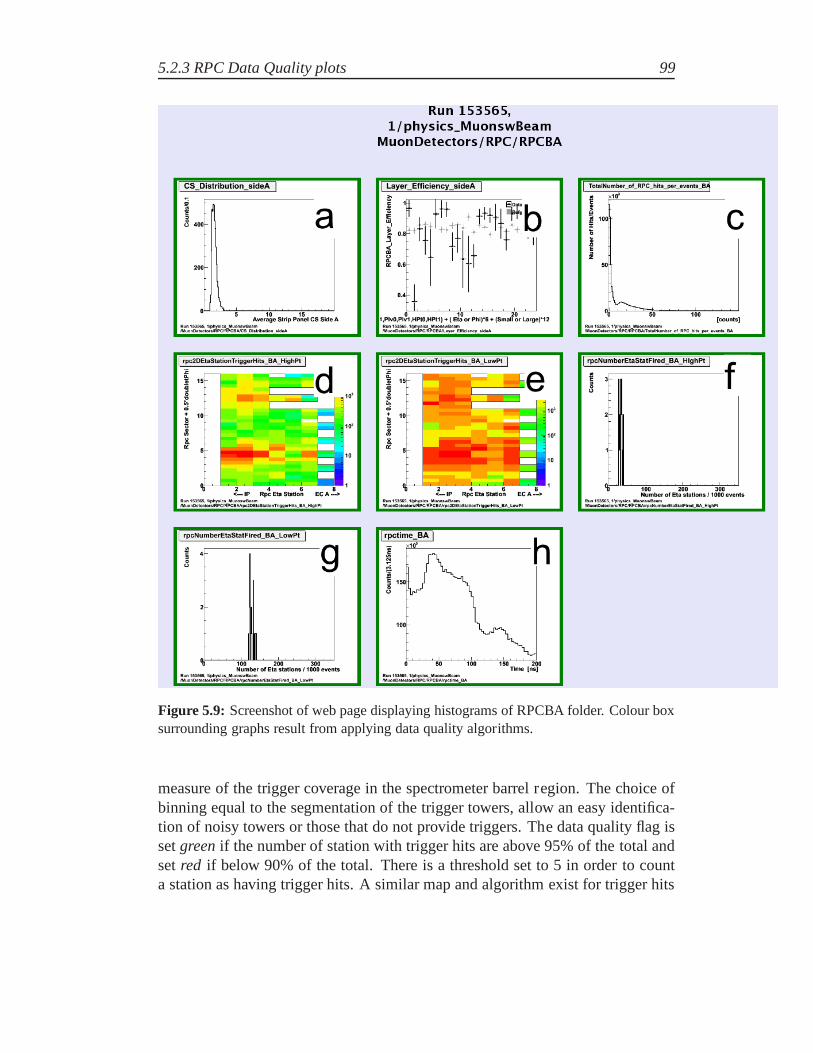
5.2.3 RPC Data Quality plots 99
Figure 5.9: Screenshot of web page displaying histograms of RPCBA folder. Colour boxsurrounding graphs result from applying data quality algorithms.
measure of the trigger coverage in the spectrometer barrel region. The choice ofbinning equal to the segmentation of the trigger towers, allow an easy identifica-tion of noisy towers or those that do not provide triggers. The data quality flag issetgreenif the number of station with trigger hits are above 95% of thetotal andsetred if below 90% of the total. There is a threshold set to 5 in orderto counta station as having trigger hits. A similar map and algorithmexist for trigger hits

100 RPC Data Quality
generated by HighPt coincidence (figure5.9(e)).
The plot of Figure5.9(f) and 5.9(g) are filled each time that a data block isclosed with the number of the RPCη stations (of respectively pivot and highpT
plane) that have at least one trigger hit. For a run with stable and uniform triggerand readout system, this number is expected to be constant and the distributionshould be very narrow. The data quality flag is setgreen if the spread in thenumber of responding station is below 15 and setred if above 30 .
The plot of Figure5.9(h) shows the distribution of the raw hit times withoutany selection. During the commissioning with cosmics the RPC readout windowsize is set to the largest size of 200 ns (eight bunch-crossing). Cosmic muons ar-rive randomly with respect to the bunch-crossing clock and the time distributionis flat inside the time window (25 nsec) of the bunch crossing window selected bythe trigger. After RPC time adjustment a single uniformly populated bunch cross-ing is expected. During beam collisions, the muons producedby the interactionarrive synchronous with the bunch-crossing clock and a verytight distribution in-side a single bunch crossing expected. The data quality flag is set GREEN if thetime spread is less than 45 ns and set RED if above 60 ns.
Figure 5.10: Screenshot of the web interface to the data quality flags database. Theoff-line flags for the all technologies of four ATLAS subdetectors are shown, each onesegmented in side A/C. On the left is shown the luminosity block validity range of theflags.
Detector off-line flags obtained from a ATLAS physics run areshown in figure5.10.

5.3 Summary plots 101
5.3 Summary plots
The monitoring package produces several histograms which summarize for eachsector the average and the spread of the main readout panel quantities. These“summary” histograms are one dimensional histograms and, on the x-axis, onebin corresponds to one RPC read-out panel and the correlation between panelindex (in the histogram) and physical coordinates ( defined at pag.66) is done bythe formula:
index =[
view + (gasgap− 1) ∗ 2 + (doubletPhi − 1) ∗ 4+ (doubletZ − 1) ∗ 8 + Plane ∗ 24+ abs(StationEta) ∗ 72
]
∗ sign(StationEta)(5.1)
Plane is 0 for LowpT panels, 1 for Pivot and 2 for High Pt. With this choicethe readout panel of Side A (positive bins) and C (negative bins) are clearly sep-arated and the eta readout panel is followed by the corresponding phi readoutpanel.
The monitored basic quantities characterizing the RPC detector response andshown by summary plots are the following:
• readout panel efficiency
• gas volume efficiency
• average readout panel cluster size
• average readout panel spatial residual for cluster size 1
• average readout panel spatial residual for cluster size 2
• average readout panel spatial residual for cluster size larger than 2
• average readout panel spatial resolution for cluster size 1
• average readout panel spatial resolution for cluster size 2
• average readout panel spatial resolution for cluster size larger than 2
• average readout panel time
• average readout panel occupancy
• average readout panel correlated noise
• average readout panel total noise
With the summary histograms, it is possible not only to spot the presenceof a problem, but also to investigate which panel has a problematic behaviourregarding to quantities listed above.
Another crucial task of summary histograms is the storing panel informationsthat has to be written in thedetector conditions database.

102 RPC Data Quality
The effective RPC working parameters (efficiency, noise andcluster size) aremeasured by using the summary histograms with the read-out panel granularityand then are stored, run by run, in a database. This allows to know the real op-erational conditions, which must be used to simulate, in Monte Carlo production,the detector response more realistic than possible. In fact, all physical measureswill be weighted by detector parameters to spot the systematic uncertainties onmeasures.
One example of summary plot is shown in figure5.11(a)where the measuredquantity is the average readout panel efficiency with its error.
In addition to the summary plots, for each sector and for physical quantities ofinterest, distribution plots are made. One example is shownin the figure5.11(b)for the efficiency. More precisely, the summary plot distribution per sector areevaluated for the previous quantities and for the spatial residuals spread for clustersize one, two and bigger than two, for a total of thirteen summary distributionplots.
Furthermore, histograms showing the distribution for sideA and C separatelyof all the above quantities are also produced.
Summary histograms like the previous ones but relative to the single RPCstrip instead to one readout panel are also available. This plots shows all the strips(both Eta and Phi views) along the X axis of a geometrical sector layer with aspecific doublet Phi. These fully detailed histograms are not generally produced(except one) in standard reconstruction process at Tier-0,because the huge amountof memory required, but are only used by detector expert for very detailed RPCcontrols.The only histogram with strip granularity produced at tier-0 contains the strip hitcounts (strip profile plot) and it is used for the evaluation of noisy and dead stripsby counting, at the end of run, the number of bin entries with respect to the totalnumber of events.An example of profile plot is shown in the Figure5.12.
Results about the evaluation of the fraction of dead strips in RPC detector willbe discussed in section6.2.1.
Histograms merging procedure
Data belonging to one run are stored in thousands of data files(because ATLASDAQ collect and store data in files which for safety reason cannot be more largethan 2 GB) which are analysed separately by the monitor code.In order to usethe full run statistics a merging procedure starts automatically at tier-0 computingfarm when the data run processing is finished. The merging procedure by defaultadd bin by bin the content of the same sub-histograms.
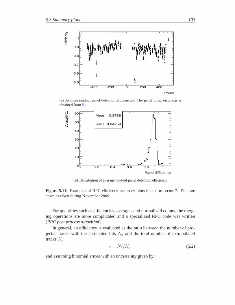
5.3 Summary plots 103
Panel
-400 -200 0 200 400
Effic
ienc
y
0.5
0.6
0.7
0.8
0.9
1
(a) Average readout panel detection efficiencies. The panelindex on x axis isobtained from5.1.
Mean 0.8765
RMS 0.04959
Panel Efficiency
0 0.2 0.4 0.6 0.8 1
Cou
nts/
0.01
0
10
20
30
40
50
60Mean 0.8765
RMS 0.04959
(b) Distribution of average readout panel detection efficiency
Figure 5.11: Examples of RPC efficiency summary plots related to sector 7.Data arecosmics taken during November 2009.
For quantities such as efficiencies, averages and normalized counts, the merg-ing operations are more complicated and a specialized RPC code was written(RPC post process algorithm).
In general, an efficiency is evaluated as the ratio between the number of pro-jected tracks with the associated hitsNh and the total number of extrapolatedtracksNp:
ǫ = Nh/Np. (5.2)
and assuming binomial errors with an uncertainty given by:

104 RPC Data Quality
strip
-800 -600 -400 -200 0 200 400 600 800
Hit
coun
ts
0
500
1000
1500
2000
2500
Figure 5.12: Examples of RPC single strip profile plot (obtained from November 2009cosmics data) .
σǫ =
√
Nh
Np
√
1 − Nh
Np
√
1
Np=
√
ǫ(1 − ǫ)
Np. (5.3)
The quantitiesNh andNp are merged by the regular add operation and fromthem theRPC post process algorithmevaluated the efficiencies with the errors.
For the average quantitiesvalue and their spread we have available the relativeextensive quantities needed to evaluate the average and thespread: the sum of theentriesNentries, the sum of the valuesNvalue and the sum of the squared valuesNsquare. These quantities could be merged by the regular add operation and theRPC post process algorithmfrom them evaluates the average, the average of thesquare and the spread by the following formula:
Nentries =∑
i=1
(entries)i (5.4)
value =Nvalue
Nentries=
∑Nentries
i=1 (value)i
Nentries(5.5)
value2 =Nsquare
Nentries=
∑Nentries
i=1 (valuei)2
Nentries(5.6)
spread =
√
value2 − value2
(5.7)

5.3 Summary plots 105
The bin content and its error are set equal to the average and the spread of thequantity respectively. Similarly, the occupancy and the noise quantities are evalu-ated by the corresponding unnormalised plots divided by thetotal event number.The readout panel summary, the sector distribution, the data quality distributionsand the single strip summary are then re-computed to accountfor the final esti-mate of those values by theRPC post process algorithm. The summary plots andthe distribution plots are filled with significant quantities only at the end of theprocess.
These kind of merging technique required to add several additional auxiliaryhistograms which are memory consuming and then a careful optimisation had tobe taken into account.
Finally, after the end of merging procedure, a dedicaded module of RPC postprocessalgorithm write out the summary results (average efficiency, clusters size,timing, etc.) for each panel in a database.

106 RPC Data Quality

6Performance of ATLAS RPC detector
6.1 Introduction
In this chapter will be presented a detailed discussion about the results on theanalysis of the RPC performance. This analysis was performed both using cosmicray data taken during the commissioning period (from the endof the installationin the cavern until the starting of the beam operation in autumn of 2009) and beamdata, particularly data registered in special runs with theso-called “beam splashevents”. In addition, in November 2009, to characterize thedetector response atthe starting of the physics program of ATLAS experiment and to know the trendof fundamental parameters (like efficiency and cluster size) as function of electricfield applied to RPC, several runs with high voltage set to different values weretaken (RPC high voltage “scan”). This is important also to check if RPC wereoperated at the proper working point.
All the results were obtained by running the RPC monitoring package, de-scribed in previous chapter4. In some cases, to perform a more detailed analysisthan that allowed at CERN-Tier0 facility, the package was run in private prepro-cessing sessions, using the CERN computing farm dedicated to users analysis andusing the worldwide distributed computing resources system called GRID. Forthis purpose, dedicated scripts were developed. The distribution plots showed be-low were obtained from ntuples dumped out by database file produced by the RPCpost-process tool (section5.3). This method allows to store the relevant RPC oper-ation parameter (efficiency, cluster size, etc.) for each read-out panel in a file withdatabase structure. Therefore, it was easy to manage a largeamount of data, tomake statistical analysis over detector properties, to apply cuts on data and makecomparisons.
6.2 Studies with cosmics data
A commissioning effort has been on-going by taking data withcosmics rays whenthe first sub-detectors were partially installed in the ATLAS pit [44, 45]. This final
107
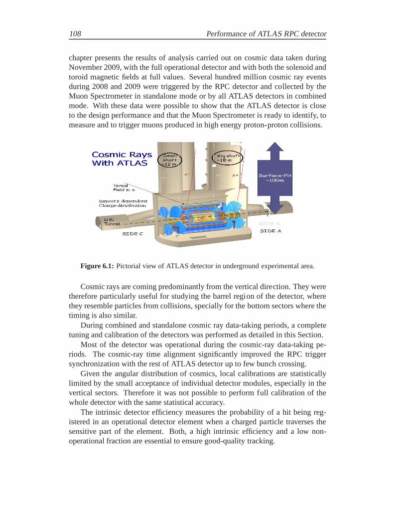
108 Performance of ATLAS RPC detector
chapter presents the results of analysis carried out on cosmic data taken duringNovember 2009, with the full operational detector and with both the solenoid andtoroid magnetic fields at full values. Several hundred million cosmic ray eventsduring 2008 and 2009 were triggered by the RPC detector and collected by theMuon Spectrometer in standalone mode or by all ATLAS detectors in combinedmode. With these data were possible to show that the ATLAS detector is closeto the design performance and that the Muon Spectrometer is ready to identify, tomeasure and to trigger muons produced in high energy proton-proton collisions.
Figure 6.1: Pictorial view of ATLAS detector in underground experimental area.
Cosmic rays are coming predominantly from the vertical direction. They weretherefore particularly useful for studying the barrel region of the detector, wherethey resemble particles from collisions, specially for thebottom sectors where thetiming is also similar.
During combined and standalone cosmic ray data-taking periods, a completetuning and calibration of the detectors was performed as detailed in this Section.
Most of the detector was operational during the cosmic-ray data-taking pe-riods. The cosmic-ray time alignment significantly improved the RPC triggersynchronization with the rest of ATLAS detector up to few bunch crossing.
Given the angular distribution of cosmics, local calibrations are statisticallylimited by the small acceptance of individual detector modules, especially in thevertical sectors. Therefore it was not possible to perform full calibration of thewhole detector with the same statistical accuracy.
The intrinsic detector efficiency measures the probabilityof a hit being reg-istered in an operational detector element when a charged particle traverses thesensitive part of the element. Both, a high intrinsic efficiency and a low non-operational fraction are essential to ensure good-qualitytracking.

6.2.1 RPC coverage 109
The intrinsic efficiencies of the RPC detectors are measuredby extrapolatingwell-reconstructed tracks through the detector and counting the numbers of hits(clusters) on the track and holes where a hit would be expected but is not found.
The measured inefficiency contains instead a contribution from isolated deadstrips due to electronics inefficiency for which no correction is applied.
6.2.1 RPC coverage
In order to have a complete picture of the response of the detector, two-dimensionalmaps of the readout hits were made for all six layers of activedetector (figures6.2,6.3and6.4). Moreover, two-dimensional distributions of the response of the trig-ger detectors are also produced (figure6.5).
As explained in chapter3, the muon trigger selects muons in barrel regionidentifying them as low-pT (pT range approximately between 4 and 10 GeV/c)or as high-pT (pT range approximately from 10 to 40 GeV/c) muons. The low-pT trigger (AtlasLowPt_TriggerOut) is made in BM chambers, the signal is sentto the BO chambers (AtlasHighPt_TriggerFromLowPt) for thefinal generation ofthe trigger signal (AtlasHighPt_TriggerOut). In this context, three types of two-dimensional plots are made to monitor the trigger response of the RPC.
These two-dimensional maps are made differently, depending on the use towhich they are intended. In the plots meant for the debug of the detector, each bincorresponds to one read-out strip. In this way is easily to identify the fractions ofdetector that does not work, but non-instrumented zones do not appear in plots.The same plots are reproduced by plotting the geometrical position of the strips.This representation allows the identification of areas thatare not instrumented andfaithfully reproduces the geometry of the apparatus. Finally, but only for two-dimensional distribution of the triggers information, theplots are also producedaccording to the coordinatesη andφ, this to allow consistent comparisons withother systems of the ATLAS detector.
In order to measure quantitatively and define in detail the coverage of thedetector, all the not operated strips are identified and monitored. A strip is definedas “dead” if produces less than 5 hits on the front end for a million triggers. Infig 6.7 is shown the number of not operated strips per panel (the fraction of deadstrips is about 2% of the total strips).
6.2.2 RPC efficiency
The efficiency of the RPC detector has been calculated by using the standalonealgorithm shown in paragraph4.5. Efficiency was estimated starting from tracksreconstructed with only RPC hits and without hits belongingto RPC plane undermeasure. When a reconstructed track is extrapolated on RPC plane, a read-out

110
Per
form
ance
ofAT
LAS
RP
Cde
tect
or
(a) AtlasLowPt0 (b) AtlasLowPt1
Figure 6.2: Detector coverage of RPC LowPt layers in spring 2010 with cosmic muons data.

6.2
.2R
PC
efficie
ncy
111
(a) AtlasPivot0 (b) AtlasPivot1
Figure 6.3: Detector coverage of RPC Pivot layers in spring 2010 with cosmic muons data.

112
Per
form
ance
ofAT
LAS
RP
Cde
tect
or
(a) AtlasHighPt0 (b) AtlasHighPt1
Figure 6.4: Detector coverage of RPC Pivot layers in spring 2010 with cosmic muons data.
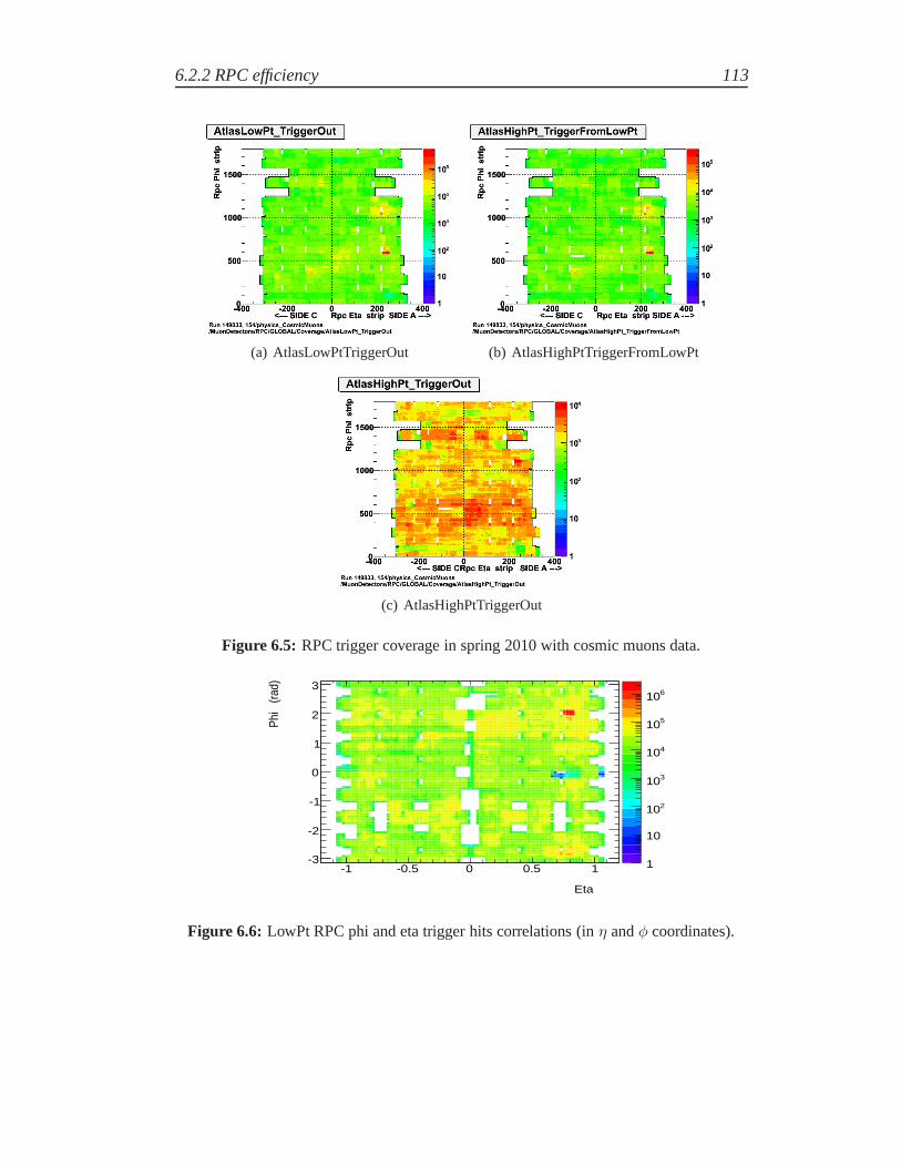
6.2.2 RPC efficiency 113
(a) AtlasLowPtTriggerOut (b) AtlasHighPtTriggerFromLowPt
(c) AtlasHighPtTriggerOut
Figure 6.5: RPC trigger coverage in spring 2010 with cosmic muons data.
Eta
-1 -0.5 0 0.5 1
Phi
(rad
)
-3
-2
-1
0
1
2
3
1
10
210
310
410
510
610
Figure 6.6: LowPt RPC phi and eta trigger hits correlations (inη andφ coordinates).

114 Performance of ATLAS RPC detector
Entries 7870Mean 0.4165RMS 2.317
# dead strips
0 5 10 15 20 25 30 35 40
Cou
nts
1
10
210
310
410Entries 7870Mean 0.4165RMS 2.317
Figure 6.7: Distribution of the number of dead strips for strip readout panel of the RPCdetector in December 2009.
electronic panel (or a strip) is declared “efficient” if there is a strip “fired” ata distance smaller than one strip from the extrapolation point. During normaloperation periods, not all RPC sectors operate at the same high voltage value,but, because temperature problems, the high voltage of the upper installed sectors(numbered 4, 5 and 6) is set to the lower value of 9400 V (instead of 9600 V). Thenot uniform conditions have to be taken into account during the data analysis.Figure6.8shows the measured ATLAS RPC panel detection efficiency, each entryis related to a single RPC readout panel. To perform an analysis on a homogeneoussample, only panels with applied high voltage at 9600 V (i.e.all sector except 4,5 and 6) and with threshold potential equal to 1 V are considered. In addition,to exclude panels not crossed by enough number of cosmic muons to make asignificant analysis, a further cut on the statistical sample is applied by requiringa number of extrapolated tracks on the panel greater or equalthan 200.
A fit with a Gaussian function performed over the efficiency distribution issuperimposed to the histogram distribution and fit parameters are showed insidethe figure.
In the same way, we can define the efficiency for the gas gap volumes.When a reconstructed track is extrapolated on RPC gas volume, we look for asignal on one of the two read-out panels (η or φ) located on the opposite side ofthe gas gap. Themeasuredgap efficiencyεgap is defined as the ratio betweenthe number of RPC signals (in at least one of the two panels) and the number ofextrapolated tracks.
The efficiency of a read-out panelεη(φ) is the product of the gap efficiencyεgap
(the probability of occurring an avalanche discharge in thegas when a muon crossit) times the read-out electronic efficiencyεη(φ)
elet (the probability that the avalanche

6.2.2 RPC efficiency 115
/ ndf 2χ 47.49 / -3Constant 15.0± 702.7
Mean 0.0005± 0.9454 Sigma 0.00047± 0.02309
Panel Efficiency
0 0.2 0.4 0.6 0.8 1
Ent
ries
[0.0
1/bi
n]
0
100
200
300
400
500
600
700
/ ndf 2χ 47.49 / -3Constant 15.0± 702.7
Mean 0.0005± 0.9454 Sigma 0.00047± 0.02309
2009 Cosmics data Preliminary ATLAS
Figure 6.8: Distribution of RPC strip readout panel average efficiency with a Gaussian fitsuperimposed.
produces a signals in read-out strips):
εη = εgap · εηelet εφ = εgap · εφ
elet . (6.1)
The quantities directly measured areεη andεφ and therefore is not possible tomeasure exactly the real gas volume efficiencyεgap,
If we defineδη andδφ as the deviations from the unity of electronic efficiencyεη
elet andεφelet:
εηelet = 1 − δη εφ
elet = 1 − δφ, (6.2)
we found that the real and the measured gap efficiency are related by:
εgap = εgap
(
1 − δηδφ)
. (6.3)
Therefore, whenδη, δφ ≈ 0 the approximation ofεgap for εgap is reasonable(in this caseδφ andδη are about 0.015).
The figure6.9 shows the distribution of ATLAS RPC gas volume averageefficiency, fitted with a Gaussian function, which parameters are reported in thebox inside the figure. Each entry in the histogram corresponds with a single RPCgas volume. Also in this case, only RPC sectors operating with high voltage at 9.6kV and threshold at 1 V are considered. As for the panel efficiency, a cut on thenumber on extrapolated tracks is applied to exclude gaps with low statistics. As

116 Performance of ATLAS RPC detector
/ ndf 2χ 49 / -3Constant 15.0± 448.6
Mean 0.0006± 0.9592 Sigma 0.00049± 0.01433
Gap Efficiency
0 0.2 0.4 0.6 0.8 1
Ent
ries
[0.0
1/bi
n]
0
50
100
150
200
250
300
350
400
450
/ ndf 2χ 49 / -3Constant 15.0± 448.6
Mean 0.0006± 0.9592 Sigma 0.00049± 0.01433
2009 Cosmics data Preliminary ATLAS
Figure 6.9: Distribution of RPC gas volume average efficiency with a Gaussian fit super-imposed.
expected, because bothη andφ signals are generated by the same avalanche, thegas volume efficiency removes some electronic inefficiency and it is greater thanthe panel efficiency.
From RPC efficiency, one can make a coarse estimation of the trigger effi-ciency. If one searches a coincidence of hits in 3 out of 4 layers, the trigger signalprobability is (if εi is the efficiency of i-th RPC panel):
ε3/4 =∏
i=1÷4
εi +∑
i=1,4
[
(
∏
j=1÷4j 6=i
εj
)(
1 − εi
)
]
. (6.4)
The formula of the trigger efficiency as function of the RPC panel efficiency ismore complicated, because trigger towers not correspond toRPC chambers (onecoincidence matrix can read signals coming from more than one RPC chamber,see pag.52). Assuming that all panels have efficiency equal to average efficiencyεi = 94.5%, we can estimate a trigger efficiency (for 3/4 majority) equal to ε3/4 =98.3%.
In order to determine the RPC intrinsic efficiency a main issues have to betaken into account. The first one is due to the fact that the RPCs are actuallyproviding the muon trigger thus resulting in a trigger bias on the efficiency cal-culation. The effect of the trigger bias has been removed from the efficiencymeasurement of an RPC plane by selecting all the events in which the other three

6.2.3 Performance from off-line monitoring 117
planes (in the case of a Middle Station) were producing hits,since the triggerrequirement is a 3 over 4 planes majority logic.
6.2.3 Performance from off-line monitoring
The developed monitoring package analyses also RPC data to check relevantquantities such as the cluster multiplicity, the occupancyand the number of noisyhits.RPC detector response is strictly dependent from environmental conditions [44],[46]. For this reason, due to the difference of temperature present in the ATLAScavern, RPC detector are operated at different high voltagevalues as a function ofy position. At the time of writing, the high voltage settingsare not yet optimized,sectors 4, 5 and 6 are operated at 9400 V, whereas the other RPCsectors are oper-ated at 9600 V. To perform an analysis over an homogeneous data sample, resultspresented in this section are obtained from run where all detector was at 9400 V.
RPC cluster size
Sometimes, a single discharge in the gas volume can induce a signal in more thanone RPC strip (i.e. occurs a so-calledcluster), this is due to the charge sharing andeventually to cross-talk phenomena1. The number of RPC strips fired in temporalcoincidence is calledcluster size. The cluster size is a relevant parameter forRPC detector and it must be strictly monitored to ensure a full trigger efficiency,it is necessary to monitor the presence of strip panels with an abnormal averagecluster size, that generally is due to front-end electronicproblems, rather than toavalanche discharge in the gas volume.
Figure6.10shows the distribution of average cluster size of all ATLAS RPCread-out strip panels, referred to 2009 December cosmics data. All panels oper-ate at same conditions of applied high voltage (9400 V) and front-end thresholdpotential (1 V).
In figure6.11the average panel cluster size is plotted as a function of sectornumber. Each point in the plot represents the average of sector distributions andthe error lines are the spread of the distributions.A dependence of average cluster size on sector angular position with respect tothe vertical cosmics is clearly visible. This is due to the fact that, when a chargedparticle cross a RPC detector not orthogonally, the chargedproduced by gas ion-isation is greater than in case of orthogonal tracks, due to the longer pattern ingas and, mainly, because the space charge effect are reduced. A greater electric
1A RPC strip is large 30 mm and, between two strips, a 0.3 mm wireis interposed to reducecross-talk phenomena.

118 Performance of ATLAS RPC detector
Entries 7534Mean 1.717RMS 0.3939
Cluster size
0 1 2 3 4 5
Cou
nts
[0.1
/bin
]
0
100
200
300
400
500
600
700
800
Entries 7534Mean 1.717RMS 0.3939
Figure 6.10: Distribution of the average cluster size of RPC strip readout panels in De-cember 2009.
charge collected on the bakelite surface can induce a more intense signal on read-out strip.
Sector
1 2 3 4 5 6 7 8 9 10 11 12 13 14 15 16
[in u
nits
of s
trip
pitc
h]Av
erag
e Pa
nel C
lust
er S
ize
1
1.2
1.4
1.6
1.8
2
2.2
2.4
2009 Cosmics data Preliminary ATLAS
Eta panelsPhi panels
sec 5,13 horizontalsec 1,9 vertical
Figure 6.11: Average cluster size of RPC strip readout panels as a function of sectornumber showing a clear dependence with respect to track inclination. Data are separatedfor η andφ panels.
For muons coming from the interaction point (almost orthogonal to RPC sur-faces of all sectors) a flat behaviour is expected with a average value close to theminimum of the present plot. Eta (Blue) and Phi (Red) panels are shown sepa-rately. Phi panels show a slightly higher cluster size than eta panels, it is expectedfrom detector construction: an additional PET (Polyethylene-Teraphtalate) sheetis inserted in between the gas volume and the eta readout panel.
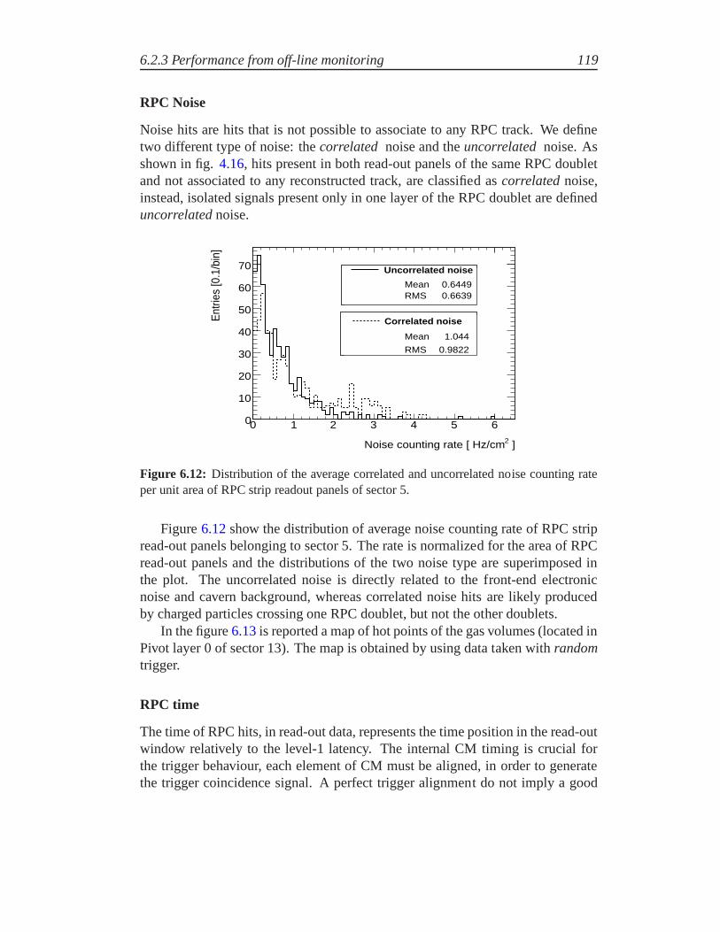
6.2.3 Performance from off-line monitoring 119
RPC Noise
Noise hits are hits that is not possible to associate to any RPC track. We definetwo different type of noise: thecorrelated noise and theuncorrelatednoise. Asshown in fig.4.16, hits present in both read-out panels of the same RPC doubletand not associated to any reconstructed track, are classified ascorrelatednoise,instead, isolated signals present only in one layer of the RPC doublet are defineduncorrelatednoise.
Mean 0.6449RMS 0.6639
]2Noise counting rate [ Hz/cm
0 1 2 3 4 5 6
Ent
ries
[0.1
/bin
]
0
10
20
30
40
50
60
70
Mean 0.6449RMS 0.6639
Mean 1.044
RMS 0.9822
Mean 1.044
RMS 0.9822
Mean 1.044
RMS 0.9822
Uncorrelated noise
Correlated noise
Figure 6.12: Distribution of the average correlated and uncorrelated noise counting rateper unit area of RPC strip readout panels of sector 5.
Figure6.12show the distribution of average noise counting rate of RPC stripread-out panels belonging to sector 5. The rate is normalized for the area of RPCread-out panels and the distributions of the two noise type are superimposed inthe plot. The uncorrelated noise is directly related to the front-end electronicnoise and cavern background, whereas correlated noise hitsare likely producedby charged particles crossing one RPC doublet, but not the other doublets.
In the figure6.13is reported a map of hot points of the gas volumes (located inPivot layer 0 of sector 13). The map is obtained by using data taken withrandomtrigger.
RPC time
The time of RPC hits, in read-out data, represents the time position in the read-outwindow relatively to the level-1 latency. The internal CM timing is crucial forthe trigger behaviour, each element of CM must be aligned, inorder to generatethe trigger coincidence signal. A perfect trigger alignment do not imply a good

120 Performance of ATLAS RPC detector
Figure 6.13: Map of the uncorrelated noise of RPC gas volumes of sector 13 side Cbelonging to pivot layer 0. The last two gas volume on the right were not triggered in thisrun.
read-out alignment, this is due to the fact that trigger and read-out data followdifferent path in the electronic chain. RPC monitoring package use only read-outinformation to plot RPC timing.
To this purpose, a dedicated section of the monitoring package checks andanalyses timing data of RPC hits. Figure6.14 shows the time distribution ofRPC hits for theη (fig. 6.14(a)) andϕ (fig. 6.14(b)) views. At the moment ofwriting, the RPC detector sections are not perfectly synchronised: the plot reflectsthis by showing a quite large distribution. When a final synchronisation will beoptimized, all entries should stay in a 25 ns window (a bunch crossing).
When the monitoring software reconstructs a track with RPC hits, it alsochecks the difference of the track hit time with the average of all other track hitstime. This value should be compared with the time of flight of muons betweendifferent RPC layers. When the time alignment will be completed, this check willbe a valid method, for example, to monitor the fraction of fake tracks. Figure6.15reports the distribution of this difference, obtained from2010 February data.
6.2.4 RPC Efficiency and Cluster Size as a function of highvoltage
To optimize the RPC working parameters, the efficiency and cluster size behaviouras a function of HV was monitored. All measurements were madethrough the useof the offline monitoring. In this case RPC was used as triggerdetector and detec-

6.2.4 RPC Efficiency and Cluster Size as a function of high voltage 121
Mean 106.7
RMS 38.32
Time Eta View [ns]
0 20 40 60 80 100 120 140 160 180 200
Cou
nts/
(3.1
25ns
)
500
1000
1500
2000
2500
3000310× Mean 106.7
RMS 38.32
(a) η hits time distribution
Mean 106.7
RMS 39.51
Time Phi View [ns]
0 20 40 60 80 100 120 140 160 180 200
Cou
nts/
(3.1
25ns
)
500
1000
1500
2000
2500
3000
3500
310× Mean 106.7
RMS 39.51
(b) φ hits time distribution
Figure 6.14: Time distribution of RPC signals in February 2010 cosmics run for η andφ
hits.
Mean 0.0002491
RMS 15.43
Track Time Residual [ns]
-100 -80 -60 -40 -20 0 20 40 60 80 100
Cou
nts/
(3.1
25ns
)
0
200
400
600
800
1000
1200
1400
1600
1800310× Mean 0.0002491
RMS 15.43
Figure 6.15: Distribution of the differences between hit time and the average time for hitsof the same track. Values are not corrected for the time of flight.
tor under measurements. In order to not introduce a bias in the measure due to thetrigger selection, during the track reconstruction the layer under measurementswas removed and hits in at least 3 layers are always required.
Figure6.16shows an example of this measurement: the RPC detection effi-ciency as a function of HV for two readout panels of separatedviews faced tothe same gas volume. The data are cosmics taken with magneticfield on. Thefront-end discrimination threshold was set at the standardvalue of Vth=1 V. Thegas volume efficiency, as calculated in paragraph6.2.2, as a function of HV isshown in figure6.17.
All curves were fitted with the following equation:

122 Performance of ATLAS RPC detector
High Voltage [V]
8600 8800 9000 9200 9400 9600
Effi
cien
cy
0.2
0.4
0.6
0.8
12009 Cosmics data
Preliminary ATLAS
Eta panels
Phi panels panelsη 0.003±= 0.974 plateauε 7) V± = (8904 1/2V
20) V± = (620 90%10%∆
panelsφ 0.003±= 0.976 plateauε 7) V± = (8938 1/2V
20) V± = (640 90%10%∆
Figure 6.16: RPC average detection efficiency of two orthogonal strip readout panels ofthe same gas volume as a function of the applied high voltage.
High Voltage [V]
8600 8800 9000 9200 9400 9600
Effi
cien
cy
0.2
0.4
0.6
0.8
12009 Cosmics data
Preliminary ATLAS
0.003 ±= 0.974 plateauε 7) V± = (8900 1/2V
20) V± = (620 90%10%∆
Figure 6.17: RPC average gas volume efficiency as a function of the appliedhigh voltage.
ε(V ) =εplateau
1 + 81
V1/2
−V
∆9010
, (6.5)
whereεplateau is the efficiency reachable for infinite value of HV,V1/2 is the volt-age values at half value of maximum efficiency and∆90
10 measures the voltagedifference between the values at90% efficiency and10% efficiency.

6.2.4 RPC Efficiency and Cluster Size as a function of high voltage 123
In order to characterize the performance of the ATLAS RPC, the distributionsof the parameters of the curve used to approximate the efficiency as a function ofHV were plotted in figure6.18.
Mean 0.9451
RMS 0.03365
Plateau efficiency 0 0.2 0.4 0.6 0.8 1
Cou
nts
[0.0
1/bi
n]
0
5
10
15
20
25
30 Mean 0.9451
RMS 0.03365
(a) Distribution of plateau efficiency.
Mean 8918
RMS 73.67
high voltage value at 50% of plateau efficiency [V]7000 7500 8000 8500 9000 9500 10000
Cou
nts
[100
/bin
]
0
10
20
30
40
50
60
70
80
90 Mean 8918
RMS 73.67
(b) Distribution of high voltage value at50% of plateau efficiency.
Mean 621.3
RMS 83.51
High voltage width 10% - 90% of plateau eff. [V]0 100 200 300 400 500 600 700 800 900 1000
Cou
nts
[10/
bin]
0
2
4
6
8
10
12
14 Mean 621.3
RMS 83.51
(c) Distribution of high voltage width valueat 10% and 90% of plateau efficiency.
Figure 6.18: Distributions of the three parameters of equation6.5obtained by fitting RPCstrip readout panel efficiency plateau curve like in figure6.16.
As for the efficiency, also the behaviour of Cluster Size was monitored as afunction of HV. As show in figure6.19, the average Cluster Size increases withvoltage reaching an average value of about 1.6 for a voltage of 9600 V. This valuewas obtained with cosmic data and only for readout panels with the front-enddiscrimination threshold set at the standard value of Vth=1 V.

124 Performance of ATLAS RPC detector
Figure 6.19: Average cluster size of a RPC strip readout panel as a function of the appliedhigh voltage.
6.3 Studies with beam data
6.3.1 Beam collimator scraping events
On the 10-th of September 2008 the first events produced by single proton beamscirculating in the LHC were recorded with the ATLAS detector. In those days,just before the 20-th of September LHC disastrous uncontrolled superconductingmagnet quenching between sector 4 and 5, RPC detector coverage were about70%. Instead, after the LHC recovery, on 20-th November 2009, RPC detectorcoverage reached about 99% coverage and the new colliding beams on collimatorswere very useful to complete the commission of the RPC detector for operationbefore collisions and to perform important tasks such as detector time alignment,channel mapping, etc. Selected examples of this colliding beam will be brieflydescribed in this Section.
For reasons of detector safety, during the 2008 beam splash period the RPCwere operated at a high voltage value of 9200 V. From this firstexperience waspossible to assure that RPC could be operated safely during these events. In fact,in the second beam splash period of November 2009, the RPC detector were op-erated at the nominal high voltage value of 9600 V.
These so-called beam splash events were produced by colliding the protons onthe closest collimators located at 140 m upstream and down stream of the ATLASdetector. These collisions generated a large quantity of particles reaching all partsof ATLAS and illuminating the whole detector at once (a schematic representationis shown in figure6.20).
As an example, figure6.21shows the spatial correlation between eta and phihits firing on the middle station of RPC detector during a “beam splash” event hit-

6.3.1 Beam collimator scraping events 125
Figure 6.20: Schematic representation of a “beam splash” event producedin the ATLASdetector by beam induced collimator scraping.
ting the whole volume of the ATLAS detector. In this event, the beam was comingfrom the right side and an attenuation along the negative z axis direction is clearlyvisible due to the particle flux absorption by ATLAS material. In particularly, inthe region near the feet the particle flux absorption is even more pronounced withrespect to the other parts. In fact, the most massive objectstraversed by the muonsare around the ATLAS feet.
Figure 6.21: RPC hit map during a “beam splash” event in December 2009 withsinglebeam from side A.
Important information for the detector start-up can be extracted from suchevents. For example, the timing setting for each channel of the electronics readout,determined beforehand from cable length and from cosmic rays, can be comparedto those obtained from the beam-splash particles. The largeamount of secondaryparticles produced by interactions of protons with collimators and traversing the
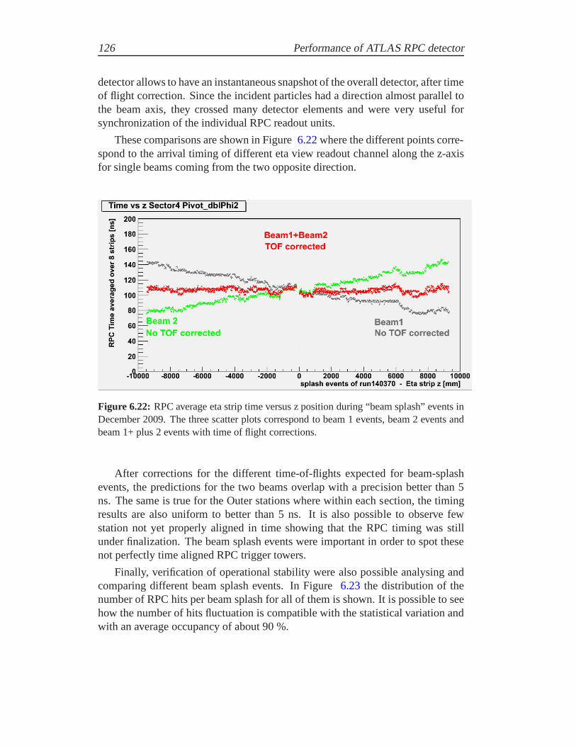
126 Performance of ATLAS RPC detector
detector allows to have an instantaneous snapshot of the overall detector, after timeof flight correction. Since the incident particles had a direction almost parallel tothe beam axis, they crossed many detector elements and were very useful forsynchronization of the individual RPC readout units.
These comparisons are shown in Figure6.22where the different points corre-spond to the arrival timing of different eta view readout channel along the z-axisfor single beams coming from the two opposite direction.
Figure 6.22: RPC average eta strip time versus z position during “beam splash” events inDecember 2009. The three scatter plots correspond to beam 1 events, beam 2 events andbeam 1+ plus 2 events with time of flight corrections.
After corrections for the different time-of-flights expected for beam-splashevents, the predictions for the two beams overlap with a precision better than 5ns. The same is true for the Outer stations where within each section, the timingresults are also uniform to better than 5 ns. It is also possible to observe fewstation not yet properly aligned in time showing that the RPCtiming was stillunder finalization. The beam splash events were important inorder to spot thesenot perfectly time aligned RPC trigger towers.
Finally, verification of operational stability were also possible analysing andcomparing different beam splash events. In Figure6.23 the distribution of thenumber of RPC hits per beam splash for all of them is shown. It is possible to seehow the number of hits fluctuation is compatible with the statistical variation andwith an average occupancy of about 90 %.

6.3.2 Beams collisions 127
Figure 6.23: RPC hit multiplicity distribution during “beam splash” events in December2009.
6.3.2 Beams collisions
This section briefly illustrate the RPC response during the December 2009 proton-proton collisions at 0.9 TeV centre of mass energy.
The spectrometer identification algorithms were optimized, for the reconstruc-tion of high-pT prompt muons and the rejection of the soft components which aredominant in the sample collected at 0.9 TeV. The MDTs, TGCs and RPCs wereall operating normally during beam collisions.
The algorithms used for muon reconstruction combine tracksfrom the muonsystems and the inner detector, but for the results presented here, two indepen-

128 Performance of ATLAS RPC detector
dent algorithms are used and only candidates selected by both are accepted. Thekinematic distributions for these candidates are presented in 6.24.
The muon spectrum observed is soft and strongly peaked in theforward di-rection, where the momentum is significantly higher for a given pT and moreeasily exceeds the average energy loss in the calorimeters of about 3.2 GeV. Theobtained kinematic distributions are compared to the predictions from minimumbias simulation with the Monte Carlo normalized to the number of muons foundin data. Within the large statistical uncertainties good agreement is found indi-cating a reasonable understanding of the initial performance of the ATLAS muonspectrometer [47].
The momentum range is problematic for the muon trigger, whose acceptanceis limited for muons in this low pT region, especially in the barrel region. Never-theless, a clear correlation could be seen between RPC trigger hits in theη andφview and the muon track reconstructed by the inner detector alone. This correla-tion is reported in the Figure6.25.
Figure 6.24: The distribution of eta and pt of reconstructed muons in December 0.9 TeVcollisions in data and simulation.
In April 2010 LHC started its first long term run at half designenergy of 7TeV centre of mass energy accumulating integrated luminosity up to few fb−1
until the end of 2011. The ATLAS detector early data analysiswill consist in“re-discovering” standard model physics in order to calibrate and extract detectorefficiency and performance from real data. The most important particle ’candle’for the muon spectrometer and the electromagnetic calorimeter is the Z bosondecaying in muons and electrons respectively and, in general, charmonium andbottomonium resonances. During the writing of this thesis the accumulated inte-grated luminosity is about an order of magnitude too low to detect the Z boson in

6.4 Conclusions 129
Figure 6.25: Azimuthal correlation (a) and in pseudo-rapidity (b) between RPC triggerhits and inner detector tracks in a sub-sample of December 2009 collisions at 0.9 TeVcentre of mass energy.
one of the lepton channels taking into account also background suppression cuts.Nevertheless, this allows for about one W boson event in one vent in both leptonschannel. In fact, a W boson candidate for the muon and for the electron channelwas recorded. In Figure6.26the first W boson candidate in the muon channel isshown with two different visualization packages. The clearW signature is evidentin this event display: in the transverse plane a back-to-back muon and missingenergy of about one third of the W mass.
6.4 Conclusions
The end of the installation of the ATLAS RPC detector in August 2008 was fol-lowed by a period of commissioning and calibration with cosmics in 2008 and2009.
During this period the detector took data with high efficiency first with cosmicrays then finally with LHC single beams and collisions. Thesedata allowed fulltests of trigger, data-acquisition, and reconstruction algorithms and monitor thesystem. Many detector properties were measured such as: occupancy, efficiency,cluster size and noise. The different RPC detector modules were timed in with aprecision of few nsec inside modules and of few bunch-crossing between modules.
The observed performance on this early data showed that the ATLAS RPCDetector is fully operational and will provide high-quality triggering and trackingfor LHC collisions.

130 Performance of ATLAS RPC detector
(a) Event display from VP visualization package.
(b) Event display Persint visualization package.
Figure 6.26: Event display of the first W boson muon-neutrino decay candidate foundin April 2010 7 TeV collisions leaving a clear muon track in the Muon Spectrometer andtransverse missing energy in the calorimeter. The two pictures correspond to the sameevent represented graphically by two different visualization software.

Summary and Outlook
ATLAS is a general purpose experiment designed to discoverynew phenomenaat the proton-proton collisions of the Large Hadron Collider built at CERN inGeneva. The ATLAS collaboration designed and built a high performance AirCore Toroidal Muon Spectrometer, in order to minimize the muon multiple scat-tering. In the barrel region of the Muon Spectrometer Resistive Plate Chambers(RPCs) are used as trigger detectors. The RPC detector was installed and operatedduring the last three years. The deep knowledge of the 4000 m2 RPC detector andthe complete control and understanding of its performancesare essential to pro-vide a reliable muon trigger.
For this work thesis a versatile software was developed to provide a detaileddetector monitoring, to perform an accurate detector characterization and to assesdetector data quality. The RPC off-line monitoring covers basic aspects of the AT-LAS RPC detector, such as: electronics channels and readoutstrip response, stan-dalone tracking capability, trigger related quantities (timing, trigger coincidencepattern and trigger road) and correlations between triggerand tracking chambers.In addition, main RPC detector performances, such as: efficiencies, cluster mul-tiplicity, residuals and noise, are measured without relying on the full ATLASreconstruction.
A big effort was also devoted to develop a coherent Data Quality frameworkbased on the information provided by the RPC off-line monitoring. Data qualityis a crucial issue for detector maintenance and physics analysis.
RPC Data Quality is done both in the on-line and off-line monitoring. Thisthesis is focused on RPC off-line Data Quality. The RPC off-line Data Qualityframework perform checks mainly on the following quantities:
• Trigger Coverage
• Detection efficiency
• Cluster multiplicity
• Noise level
• Time alignments
131

132 Performance of ATLAS RPC detector
• Stability
Automatics quality checks are based on histograms and applying specific al-gorithms. To allow an easy and fast data quality evaluation,the histograms andalgorithm results are displayed on-line by a common ATLAS framework basedon dynamic web pages. A subset of dynamic pages specific to RPCdetector wasrealized in this work thesis. This allowed also to store automatically the RPC DataQuality flags in the common ATLAS Database.
Finally the analysis of RPC cosmic data collected at the end of the commis-sioning phase is also presented together with the first beam scraping test and col-lisions events. In particular, a complete detector efficiency scan is shown in greatdetails and the best working point "in situ" found. The results of these studiesshown the good performance of the RPC detector as muon trigger in the LHCenvironment with high coverage, high efficiency and low noise.

Bibliography
[1] F. Halzen and A. D. Martin. QUARKS AND LEPTONS: an introductorycourse in modern particle physics. John Wiley and Sons, New York, 1984.
[2] C. Amsler et al. (Particle Data Group). The Review of Particle Physics.Physics Letters, B667, 2008.
[3] S. L. Glashow. Partial Symmetries of Weak Interactions.Nucl. Phys.,22:579–588, 1961.
[4] P. W. Higgs. BROKEN SYMMETRIES AND THE MASSES OF GAUGEBOSONS.Phys. Rev. Lett., 13:508–509, 1964.
[5] C. Amsler et al. (Particle Data Group). The Review of Particle Physics.Physics Letters, B667, 2008.
[6] V.M. Abazov et al. A combined search for the standard model higgs bosonat√s = 1.96 TeV. Physics Letters B, 663(1-2):26 – 36, 2008.
[7] Combined CDF and D0 Upper Limits on Standard Model Higgs-Boson Pro-duction with 2.1 - 5.4 fb-1 of Data. 2009.
[8] CERN. oai:cds.cern.ch:1021125. PHYSTAT-LHC Workshop on StatisticalIssues for LHC Physics, Geneva, 2008. CERN.
[9] ATLAS detector and physics performance: Technical Design Report, 2.Technical Design Report ATLAS. CERN, Geneva, 1999. Electronic versionnot available.
[10] J. F. Gunion, Howard E. Haber, and C. Kao. Searching for thecp-odd higgsboson of the minimal supersymmetric model at hadron supercolliders. Phys.Rev. D, 46(7):2907–2917, Oct 1992.
[11] D. Cavalli, D. Froidevaux, F. Gianotti, L. Poggioli, S.Resconi, andE. Richter-Was. Minimal supersymmetric standard model higgs rates andbackgrounds in atlas. Technical Report ATL-PHYS-96-074. ATL-GE-PN-74, CERN, Geneva, Apr 1996.
133

134 BIBLIOGRAPHY
[12] E. Richter-Was and D. Froidevaux. Mssm higgs bosons in sugra model:observability in sm decay modes with atlas. Technical Report ATL-COM-PHYS-98-012, Nov 1998.
[13] T. S. Pettersson and P. Lefèvre. The large hadron collider: conceptual design.oai:cds.cern.ch:291782. Technical Report CERN-AC-95-05LHC, CERN,Geneva, Oct 1995.
[14] The ATLAS collaboration. The ATLAS Experiment at the CERN LargeHadron Collider.JINST, 3:S08003, 2008.
[15] ATLAS magnet system: Technical Design Report, 1. Technical Design Re-port ATLAS. CERN, Geneva, 1997.
[16] ATLAS inner detector: Technical Design Report, 1. Technical Design ReportATLAS. CERN, Geneva, 1997.
[17] S. Haywood, L. Rossi, R. Nickerson, and A. Romaniouk.ATLAS innerdetector: Technical Design Report, 2. Technical Design Report ATLAS.CERN, Geneva, 1997.
[18] M. S. Alam et al. The atlas silicon pixel sensors.Nuclear Instruments andMethods in Physics Research Section A: Accelerators, Spectrometers, De-tectors and Associated Equipment, 456(3):217 – 232, 2001.
[19] ATLAS liquid-argon calorimeter: Technical Design Report. Technical De-sign Report ATLAS. CERN, Geneva, 1996.
[20] ATLAS tile calorimeter: Technical Design Report. Technical Design ReportATLAS. CERN, Geneva, 1996.
[21] ATLAS Muon Collaboration. Atlas muon spectrometer technical design re-port. 1997.
[22] ATLAS detector and physics performance: Technical Design Report. Tech-nical Design Report ATLAS. CERN, Geneva, 1999.
[23] W. Blum. High-recision drift tubes. Technical Report ATL-MUON-93-024.ATL-M-PN-24, CERN, Geneva, Jul 1993.
[24] N. C. Benekos, D. G. Drakoulakos, C. W. Fabjan, V. P. Falaleev,Z. Krumshtein, F. Lejal, J. M. Maugain, S. Rangod, F. Rohrbach, Y. V.Sedykh, and L. S. Vertogradov. Xtomo2, stereo-measurements of the mdtmuon chambers using a high precision x-ray tomograph. Technical ReportATL-MUON-97-155. ATL-M-PN-155, CERN, Geneva, Apr 1997.
BIBLIOGRAPHY 135
[25] V. Paschhoff and M. Spegel. Ageing studies for the atlasmdt’s using ar-co290-10. Technical Report ATL-MUON-2000-004, CERN, Geneva,Jun 1999.
[26] M. Dikken. The rasnik in-plane alignment system. Technical Report ATL-MUON-97-184. ATL-M-PN-184, CERN, Geneva, 1997.
[27] E. Duchovni, T. Kobayashi, D. Lellouch, L. Levinson, N.Lupu, T. Mashimo,G. Mikenberg, and M. Shoa. Possible utilization of thin-gapchambers in theatlas muon system. Technical Report ATL-MUON-93-023. ATL-M-PN-23,CERN, Geneva, Jun 1993.
[28] K. Nagai. Thin gap chambers in ATLAS.Nucl. Instrum. Meth., A384:219–221, 1996.
[29] V. Smakhtin. Testing TGC detectors in a high rate environment. Nucl. In-strum. Meth., A494:500–503, 2002.
[30] R. Santonico and R. Cardarelli. Development of resistive plate counters.Nuclear Instruments and Methods, A(377):187, 1981.
[31] R. Cardarelli, V. Makeev, and R. Santonico. Avalance and streamer modeoperation of resistive plate chambers.Nuclear Instruments and Methods,1996.
[32] G. Aielli, P. Camarri, R. Cardarelli, A. Di Ciaccio, L. Di Stante, B. Liberti,A. Paoloni, E. Pastori, and R. Santonico. Test of atlas rpcs front-end elec-tronics. Nuclear Instruments and Methods in Physics Research Section A:Accelerators, Spectrometers, Detectors and Associated Equipment, 508(1-2):189 – 193, 2003. Proceedings of the Sixth International Workshop onResistive Plate Chambers and Related Detectors.
[33] F. Giannini, E. Limiti, G. Orengo, and R. Cardarelli. An8 channel GaAs ICfront-end discriminator for RPC detectors.Nuclear Instruments and Meth-ods in Physics Research Section A: Accelerators, Spectrometers, Detectorsand Associated Equipment, 432(2-3):440 – 449, 1999.
[34] ATLAS computing: Technical Design Report. Technical Design Report AT-LAS. CERN, Geneva, 2005.
[35] G. Barrand et al. Gaudi – a software architecture and framework for build-ing hep data processing applications.Computer Physics Communications,140(1-2):45 – 55, 2001.

136 BIBLIOGRAPHY
[36] P. Jenni, M. Nessi, M. Nordberg, and K. Smith.ATLAS high-level trigger,data-acquisition and controls: Technical Design Report. Technical DesignReport ATLAS. CERN, Geneva, 2003.
[37] A. Corso-Radu, S. Kolos, H. Hadavand, R. Kehoe, and M. Hauschild.Data quality monitoring framework for the atlas experimentat the lhc.Technical Report ATL-DAQ-CONF-2008-006. ATL-COM-DAQ-2007-033,CERN, Geneva, Oct 2007.
[38] ATLAS level-1 trigger: Technical Design Report. Technical Design ReportATLAS. CERN, Geneva, 1998.
[39] V. Bocci, E. Petrolo, A. Salamon, R. Vari, and S. Veneziano. The design ofthe coincidence matrix asic of the atlas barrel level-1 muontrigger. 2002.
[40] N. Benekos, M. Bianco, G. Chiodini, I. A. Christidi, J. Coggeshall,A. Cortes-Gonzalez, E. Gorini, D. Fortin, J. Griffiths, A. Guida, et al. Muonoffline monitoring at tier0 using cosmics and fdr data. Technical ReportATL-COM-MUON-2009-042, CERN, Geneva, Nov 2009.
[41] M. Baak, C. Guyot, M. Hauschild, R. Hawkings, B. Heinemann, A. Hocker,M. Martínez-Pérez, D. Malon, P. Onyisi, and E. Torrence. Data quality statusflags and good run lists for physics analysis in atlas. Technical Report ATL-COM-GEN-2009-015, CERN, Geneva, Mar 2009.
[42] A. Corso-Radu, S. Kolos, H. Hadavand, R. Kehoe, and M. Hauschild.Data quality monitoring framework for the atlas experimentat the lhc.Technical Report ATL-DAQ-CONF-2008-006. ATL-COM-DAQ-2007-033,CERN, Geneva, Oct 2007.
[43] L. W. Alvarez. A proposal to “X-Ray” the egyptian pyramids to search forpresently unknown chambers.LBNL Physics notes, 544, 1965.
[44] M. Bianco. ATLAS RPC certification and commissioning with cosmic rays.PhD thesis, Lecce University, 2007.
[45] G. Chiodini et al. Rpc cosmic ray tests in the atlas experiment. Nuclear In-struments and Methods in Physics Research Section A: Accelerators, Spec-trometers, Detectors and Associated Equipment, 581(1-2):213 – 216, 2007.VCI 2007 - Proceedings of the 11th International Vienna Conference on In-strumentation.
[46] M. Bianco, G. Chiodini, E. Gorini, F. Grancagnolo, R. Perrino, M. Primav-era, and S. Spagnolo. Temperature dependent performance ofATLAS RPC.Nuclear Physics B Proceedings Supplements, 158:204–207, August 2006.

BIBLIOGRAPHY 137
[47] G. Aad et al. Charged-particle multiplicities in pp interactions at√s = 900
GeV measured with the ATLAS detector at the LHC. 2010.


