OFDM Physical Layer Architecture and Real-Time Multi-Path ...
159
OFDM Physical Layer Architecture and Real-Time Multi-Path Fading Channel Emulation for the 3GPP Long Term Evolution Downlink by Elliot Briggs, B.S.E.E., M.S.E.E. A Dissertation In Electrical Engineering Submitted to the Graduate Faculty of Texas Tech University in Partial Fulfillment of the Requirements for the Degree of Doctor of Philosophy Approved Dr. Brian Nutter Dr. Tanja Karp Dr. Sunanda Mitra Dr. Dominick Casadonte Interim Dean of the Graduate School December, 2012
Transcript of OFDM Physical Layer Architecture and Real-Time Multi-Path ...
OFDM Physical Layer Architecture and Real-Time Multi-Path FadingChannel Emulation for the 3GPP Long Term Evolution Downlink
by
Elliot Briggs, B.S.E.E., M.S.E.E.
A Dissertation
In
Electrical Engineering
Submitted to the Graduate Facultyof Texas Tech University in
Partial Fulfillment ofthe Requirements for
the Degree of
Doctor of Philosophy
Approved
Dr. Brian Nutter
Dr. Tanja Karp
Dr. Sunanda Mitra
Dr. Dominick CasadonteInterim Dean of the Graduate School
December, 2012

©2012Elliot Briggs

Texas Tech University, Elliot Briggs, December 2012
Contents
List of Tables iv
List of Figures v
Nomenclature viii
Abstract xii
1 Preface 11.1 Background . . . . . . . . . . . . . . . . . . . . . . . . . . . . . . . . . . . . . . 11.2 Acknowledgments . . . . . . . . . . . . . . . . . . . . . . . . . . . . . . . . . . 11.3 Organization . . . . . . . . . . . . . . . . . . . . . . . . . . . . . . . . . . . . . 2
2 Introduction 22.1 OFDM Receiver Synchronization and Equalization . . . . . . . . . . . . . . 32.2 System Architecture for Real-Time Multi-Path Wireless Channel Emulation 42.3 Cyclic Prefix Redundancy Combination and Arbitrary-Ratio Resampling 5
2.3.1 Cyclic Prefix Redundancy Combination with LTE Context . . . . . 52.3.2 Arbitrary-Ratio Resampling Using a Reformulated Farrow Filter . 5
2.4 Contributions . . . . . . . . . . . . . . . . . . . . . . . . . . . . . . . . . . . . 6
3 OFDM Receiver Synchronization 73.1 OFDM System Model . . . . . . . . . . . . . . . . . . . . . . . . . . . . . . . . 73.2 Timing Synchronization . . . . . . . . . . . . . . . . . . . . . . . . . . . . . . 83.3 Sampling Clock Frequency Offset and Symbol Timing Correction: A
Joint Effort . . . . . . . . . . . . . . . . . . . . . . . . . . . . . . . . . . . . . . 183.4 Time-Domain Detection of the LTE Primary Synchronization Signal . . . 243.5 Concluding Remarks . . . . . . . . . . . . . . . . . . . . . . . . . . . . . . . . 39
4 OFDM Channel Estimation and Equalization 404.1 Linear Regression Techniques for Channel Estimation . . . . . . . . . . . . 454.2 The Missing Link: Frequency-Time Interpolation . . . . . . . . . . . . . . . 584.3 Reference Symbol Arrangements and Their Relationship with Timing
Synchronization . . . . . . . . . . . . . . . . . . . . . . . . . . . . . . . . . . 714.4 Concluding Remarks . . . . . . . . . . . . . . . . . . . . . . . . . . . . . . . . 74
5 Resampling Techniques Using Locally Weighted Linear Regression 75
6 Exploitation of Excess Cyclic Prefix to Improve Reception Quality 876.1 Concluding Remarks . . . . . . . . . . . . . . . . . . . . . . . . . . . . . . . . 92
7 Real-Time Wireless Channel Emulation 947.1 Real-Time Multi-Path SISO Channel Emulation . . . . . . . . . . . . . . . . 95
7.1.1 Stochastic Jakes Process Generation . . . . . . . . . . . . . . . . . . 957.1.2 Arbitrary-Ratio Upsampler Design: User-Variable Doppler . . . . . 99
ii

Texas Tech University, Elliot Briggs, December 2012
7.2 Real-Time Milti-Path MIMO Channel Emulation . . . . . . . . . . . . . . . 1097.3 Implemention in FPGA Hardware . . . . . . . . . . . . . . . . . . . . . . . . 1157.4 Concluding Remarks . . . . . . . . . . . . . . . . . . . . . . . . . . . . . . . . 119
8 Conclusions 120
A Generic Multicarrier System Model 122A.1 Linear Transforms and Basis Functions . . . . . . . . . . . . . . . . . . . . . 122A.2 Serial-to-Parallel and Mapping . . . . . . . . . . . . . . . . . . . . . . . . . . 125A.3 The Stationary AWGN Channel . . . . . . . . . . . . . . . . . . . . . . . . . . 127
B OFDM System Model 133
References 140
iii

Texas Tech University, Elliot Briggs, December 2012
List of Tables
1 Root Indices for the LTE Primary Synchronization Signal . . . . . . . . . . 262 Multi-Rate PSS Detector Computation and Coefficient Storage Require-
ments . . . . . . . . . . . . . . . . . . . . . . . . . . . . . . . . . . . . . . . . . 333 Dyadic Cascaded Upsampler Computation and Coefficient Storage Re-
quirements . . . . . . . . . . . . . . . . . . . . . . . . . . . . . . . . . . . . . . 354 Breakdown of Computations of Overlap-Add PSS detection as Imple-
mented by MATLAB’s “fftfilt” function . . . . . . . . . . . . . . . . . . . . . . 385 Computational Breakdown for Online Computation of Locally Weighted
Linear Regression (m= 2) . . . . . . . . . . . . . . . . . . . . . . . . . . . . . 496 Coefficients of Designed Dyadic Linear Phase Half-Band IIR Upsampler . 1047 IIR and FIR Interpolation Performance Comparison . . . . . . . . . . . . . 1058 Workload and Coefficient Storage Breakdown for a Single Variable-Rate
Channel Coefficient Generator . . . . . . . . . . . . . . . . . . . . . . . . . . 1099 FPGA Resource Consumption for a Single Channel Matrix Generator, Ex-
cluding WGN Source ( fs = 200 MHz) . . . . . . . . . . . . . . . . . . . . . . 118
iv

Texas Tech University, Elliot Briggs, December 2012
List of Figures
1 FIR Filter That Models the Effects of Fractional Timing Error (M = 256) 102 Illustration of “Left” and “Right” Symbol Timing Error Positions . . . . . 113 SIR vs. Symbol Timing Error m - Left and Right Errors . . . . . . . . . . . 134 Data-Driven Critical Value for Symbol Timing Estimates . . . . . . . . . . 165 SNR Degradation vs. Subcarrier Index . . . . . . . . . . . . . . . . . . . . . 196 SNR Degradation vs. SCO with Varying Es
N0. . . . . . . . . . . . . . . . . . . 20
7 Receiver Architecture Capable of Synchronizing SCO and Symbol Timing 218 Received OFDM Signal Afflicted with 40 ppm of SCO: Effects on SNR
and Symbol Timing . . . . . . . . . . . . . . . . . . . . . . . . . . . . . . . . . 229 Received OFDM Signal Afflicted with -40 ppm of SCO After Resampling
Using Measured Timing Drift Rate and Feedback Control Technique . . . 2210 Received OFDM Signal Afflicted with -40 ppm of SCO and EVA-200
Channel Model: Successful SCO Detection and Correction Using OnlyTime-Domain Information in High Mobility Channel Conditions . . . . . 23
11 Cyclic Correlation Properties Between the LTE Downlink PSS ZC Sequences 2712 PSS Position in an LTE Downlink OFDM Symbol . . . . . . . . . . . . . . . 2713 Linear Correlation Properties Between the LTE Downlink PSS ZC Se-
quences . . . . . . . . . . . . . . . . . . . . . . . . . . . . . . . . . . . . . . . . 2914 Alias Zones Introduced by Initial 2x Downsampling in an LTE PSS Sym-
bol (NF F T = 256) . . . . . . . . . . . . . . . . . . . . . . . . . . . . . . . . . . 3015 Frequency Response of LTE Test Signal Overlaid with Oversampled PSS
Matched Filter (NF F T = 256) . . . . . . . . . . . . . . . . . . . . . . . . . . . 3016 Dyadic Downsampling Filter Response Overlay . . . . . . . . . . . . . . . . 3217 Dyadic Downsampling Filter: Cascaded Frequency Response . . . . . . . 3218 Dyadic Downsampling Filter with Matched Filter Bank: Implemented
Structure . . . . . . . . . . . . . . . . . . . . . . . . . . . . . . . . . . . . . . . 3319 Dyadic Upsampling Filter Response Overlay . . . . . . . . . . . . . . . . . . 3420 Dyadic Upsampling Filter: Cascaded Frequency Response . . . . . . . . . 3521 Multi-Rate PSS Detection Algorithm: Implemented Processing Structure 3622 Multi-Rate vs. Overlap-Add PSS Correlation . . . . . . . . . . . . . . . . . . 3723 . . . . . . . . . . . . . . . . . . . . . . . . . . . . . . . . . . . . . . . . . . . . . 3824 LMS Equalizer Results: Equalization Coefficients (top), Per-Channel Squared
Error (bottom) . . . . . . . . . . . . . . . . . . . . . . . . . . . . . . . . . . . . 4425 Exponential Weighting Kernel with Varying τ Parameter . . . . . . . . . . 5026 Overlaid Locally Weighted Regression Results with Varying τ Kernel Pa-
rameter . . . . . . . . . . . . . . . . . . . . . . . . . . . . . . . . . . . . . . . . 5127 MSE vs. Model Parameter τ . . . . . . . . . . . . . . . . . . . . . . . . . . . . 5228 LWR Experiment: Mean-Squared Error vs. τ vs. N . . . . . . . . . . . . . . 5329 MSE vs. Model Parameter τ: i.i.d. Trials with i.i.d. AWGN . . . . . . . . . 5430 Finding the Abscissa of a Quadratic Function’s Minumum Using Inverse
Quadratic Interpolation . . . . . . . . . . . . . . . . . . . . . . . . . . . . . . 5531 Finding the Abscissa of an Arbitrary Function’s Local Minumum Using
the Successive Inverse Quadratic Minimum Finding Technique . . . . . . 56
v
Texas Tech University, Elliot Briggs, December 2012
32 Successive Inverse Quadratic Inerpolation Minimum Finding AlgorithmFinding the Minimum Across the Error Surface of the LWR Kernel Pa-rameter Sweeps . . . . . . . . . . . . . . . . . . . . . . . . . . . . . . . . . . . 57
33 Frequency-Staggered, Time-Spaced Reference Symbol Orientation in the“Extended” and “Normal” CP Modes Used in the LTE Downlink . . . . . . 58
34 Valid Output Samples of a Rate-6 Polyphase Upsampler Overlaid on theKnown Channel Magnitude . . . . . . . . . . . . . . . . . . . . . . . . . . . . 64
35 Interpolation and Gap-Filling of a Periodic Signal using the ExtendedDFT Algorithm . . . . . . . . . . . . . . . . . . . . . . . . . . . . . . . . . . . . 66
36 Cubic Spline Interpolation/Extrapolation Along the Frequency Dimen-sion (Step 1) . . . . . . . . . . . . . . . . . . . . . . . . . . . . . . . . . . . . . 68
37 Cubic Spline Interpolation/Extrapolation Along the Time Dimension (Step2) . . . . . . . . . . . . . . . . . . . . . . . . . . . . . . . . . . . . . . . . . . . . 69
38 MSE of Cubic Spline Interpolation/Extrapolation Operating Under theEVA Channel Model . . . . . . . . . . . . . . . . . . . . . . . . . . . . . . . . . 70
39 Comparison Between LWR and LS Algorithms Applied to LTE RS config-uration with Cubic Splines Interpolator, EVA Channel Model, σ2 = .005 71
40 An Example Comparison of LWR vs. LS Equalization: QPSK ModulatedData, EPA-5 Channel Model . . . . . . . . . . . . . . . . . . . . . . . . . . . . 72
41 MSE Performance Comparison of LS and LWR Channel Estimators UsingLTE Channel Models . . . . . . . . . . . . . . . . . . . . . . . . . . . . . . . . 73
42 Simultaneous Data Smoothing and (4x) Interpolation Using the LWRAlgorithm (m= 4) . . . . . . . . . . . . . . . . . . . . . . . . . . . . . . . . . 76
43 Farrow Filter Structure Derived from the LWR Algorithm . . . . . . . . . . 7744 Q Matrix Row-Wise Taps (top row), Q Matrix Row-Wise Frequency Re-
sponses (bottom row), m=5, p=8, β = 30 . . . . . . . . . . . . . . . . . . . 7845 Generated CVFD (Farrow) Filter’s Group Delay vs. ∆ . . . . . . . . . . . . 7946 Generated CVFD (Farrow) Filter’s Magnitude and Phase vs. ∆ . . . . . . 7947 Q Matrix Row-Wise Taps (top row), Q Matrix Row-Wise Frequency Re-
sponses (bottom row), m= 5, p = 24,β = 250 . . . . . . . . . . . . . . . . 8048 Q Matrix Row-Wise Taps (top row), Q Matrix Row-Wise Frequency Re-
sponses (bottom row), m= 5, p = 24,β = 14 . . . . . . . . . . . . . . . . . 8149 Generated CVFD (Farrow) Filter’s Group Delay vs. ∆: m = 5, p =
24,β = 14 . . . . . . . . . . . . . . . . . . . . . . . . . . . . . . . . . . . . . . 8150 Generated CVFD (Farrow) Filter’s Magnitude vs. ∆: m = 5, p = 24,β =
14, Useful for Simultaneous Interpolation and Smoothing . . . . . . . . . 8251 Sidelobes Resulting from CVFD Rate Transition with Varying Levels of
Input Oversampledness�
m= 5, p = 8,β = 30�
. . . . . . . . . . . . . . . . 8352 Generalized CVDF (Farrow) Based Arbitrary-Ratio Upsampler Using 8x
Polyphase Upsampling Preprocessor . . . . . . . . . . . . . . . . . . . . . . . 8453 Inconvenient-Rate Resampling for an LTE or UMTS System to 100 MHz
Sampling Rate from 30.72 MHz . . . . . . . . . . . . . . . . . . . . . . . . . 8554 Farrow-Based LTE Resampling Filter . . . . . . . . . . . . . . . . . . . . . . 8655 Receiver Architecture: Combining CP Redundancy in the Time Domain . 91
vi

Texas Tech University, Elliot Briggs, December 2012
56 SNR Enhancement Using CP Redundancy in AWGN Channel and Multi-Path Channel Conditions . . . . . . . . . . . . . . . . . . . . . . . . . . . . . . 92
57 Time-Varying SISO Channel Model . . . . . . . . . . . . . . . . . . . . . . . 9658 Designed Jakes FIR Filter: NJakes = 256, fmax = 100 Hz, fd = .8 . . . . . 9859 Single MACC Element Jakes Filter Processing p Complex Jakes Processes 9960 Arbitrary-Ratio Resampler Architecture . . . . . . . . . . . . . . . . . . . . . 10061 Dyadic Half-Band 4x FIR Upsampler - Overlaid and Cascaded Frequency
Response . . . . . . . . . . . . . . . . . . . . . . . . . . . . . . . . . . . . . . . 10262 Dyadic Half-Band 2x FIR Upsampler - Implementation Structure . . . . . 10363 Second Order Type-1 and Type-2 All-Pass Sections . . . . . . . . . . . . . . 10364 An Example of Cascaded Half-Band IIR Upsamplers Constructed Using
Cascaded 2nd-Order All-Pass Sections . . . . . . . . . . . . . . . . . . . . . 10365 Dyadic Half-Band Linear Phase 4x IIR Upsampler - Overlaid and Cas-
caded Frequency Response . . . . . . . . . . . . . . . . . . . . . . . . . . . . 10466 Prototype Filter for 32x Upsampler: Exploiting the Oversampled Input
Signal (5x magnification) . . . . . . . . . . . . . . . . . . . . . . . . . . . . . 10667 Dual Polyphase Filter Arbitrary-Ratio Resampler: Dual Commutator Traver-
sal States with Extended Shift Register Positioning . . . . . . . . . . . . . . 10768 Arbitrary-Ratio Upsampler: Rate-32 Polyphase Upsampling with Linear
Interpolators . . . . . . . . . . . . . . . . . . . . . . . . . . . . . . . . . . . . . 10869 Frequency Response of the Cascaded Jakes and Arbitrary-Ratio Resam-
pler: δ = 0.0225 . . . . . . . . . . . . . . . . . . . . . . . . . . . . . . . . . . . 10870 Tapped Delay Line MIMO Channel Model . . . . . . . . . . . . . . . . . . . 11071 Channel Matrix Generator System Diagram . . . . . . . . . . . . . . . . . . 11472 Hardware Matrix Multiplication Operation for Correlating i.i.d. Jakes
Processes . . . . . . . . . . . . . . . . . . . . . . . . . . . . . . . . . . . . . . . 11573 Test Configuration of the Implemented Channel Emulator . . . . . . . . . 11674 Hardware-Sourced Jakes Impulse Response from MIMO Emulator . . . . 11775 Two-Element Vector Defined in the Orthonormal Basis
�
x0, x1
�
. . . . . . 12376 Two-Element Vector Redefined in the Orthonormal Basis
�
y0, y1
�
. . . . . 12377 x and y orthonormal basis vectors defined in the x basis . . . . . . . . . . 12478 QAM Constellations: QPSK and 16QAM . . . . . . . . . . . . . . . . . . . . 12579 Generic System Model . . . . . . . . . . . . . . . . . . . . . . . . . . . . . . . 12780 Effect of a noisy channel with memory: OFDM example . . . . . . . . . . 13281 Illustration of the Cyclic Prefix in an OFDM signal . . . . . . . . . . . . . . 13682 Generic OFDM System Model (Equalization Component not Shown) . . 139
vii

Texas Tech University, Elliot Briggs, December 2012
Nomenclature
Acronyms
3GPP 3rd Generation Partnership Project
ACF Autocorrelation Function
ADC Analog to Digital Converter
ALU Arithmetic Logic Unit
AWGN Additive White Gaussian Noise
CCF Cross Correlation Function
CFO Carrier Frequency Offset
CP Cyclic Prefix
CVDF Continuously Variable Delay Filter
DAC Digital to Analog Converter
DDS Direct Digital Synthesis
DFT Discrete Fourier Transform
DRAM Dynamic Random Access Memory
DSP Digital Signal Processing
DTFT Discrete-Time Fourier Transform
EDFT Extended Discrete Fourier Transform
EPA Extended Pedestrian A
ETU Extended Typical Urban
EVA Extended Vehicular A
FBMC Filter Bank Multicarrier
FDD Frequency Domain Duplexing
FFT Fast Fourier Transform
FIFO First In First Out
FIR Finite Impulse Response
flop Floating-Point Operation
viii

Texas Tech University, Elliot Briggs, December 2012
FPGA Field Programmable Gate Array
HARQ Hybrid Automatic Repeat Request
i.i.d. Independent and Identically Distributed
ICI Inter-Carrier Interference
IIR Infinite Impulse Response
ISI Inter-Symbol Interference
LDPC Low Density Parity Check
LMMSE Linear Minimum Mean Squared Error
LMS Least Mean Squares
LS Least Squares
LTE Long Term Evolution
LWR Locally Weighted Regression
MACC Multiply Accumulate
MATLAB Matrix Laboratory
MF Matched Filter
ML Maximum Likelihood
MMSE Minimum Mean Squared Error
MSE Mean Squared Error
MUX Multiplexer
NLMS Normalized Least Mean Squares
OFDM Orthogonal Frequency Division Multiplexing
PDP Power Delay Profile
PHY Physical Layer
ppm Parts Per Million
PRACH Physical Random Access Channel
PSD Power Spectral Density
PSS Primary Synchronization Signal
ix
Texas Tech University, Elliot Briggs, December 2012
QAM Quadrature Amplitude Modulation
QPSK Quadrature Phase Shift Keying
RAM Random Access Memory
RLS Recursive Least Squares
ROM Read-Only Memory
RS Reference Symbol
SCO Sampling Clock Offset
SERDES Serializer-Deserializer
SIR Signal to Interference Ratio
SNR Signal to Noise Ratio
SOS Sum of Sinusoids
SSS Secondary Synchronization Signal
TDD Time Domain Duplexing
UMTS Universal Mobile Telecommunications System
WGN White Gaussian Noise
WOM Write-Only Memory
ZC Zadoff-Chu
Operator
(·)(i) i th time index or iteration of vector or matrix
(·)H The Hermitian transpose of a vector or matrix
(·)T The transpose of a vector or matrix
0M×N An M × N rectangular matrix of zeros
0M An M ×M matrix of zeros
H−1 Inverse of matrix H
H:, j The contents of the j th column of matrix H
Hi,: The contents of the i th row of matrix H
Hi, j The element located in the i th row and j th column of matrix H
x

Texas Tech University, Elliot Briggs, December 2012
Hi,m:n The contents of the mth through the nth column in the i th row ofmatrix H
hi The i th element in the vector h
Hm:n, j The contents of the mth through the nth row in the j th columnof matrix H
hm:n The contents of the mth through nth element in the vector h
HM A square matrix H with dimensions M ×M
IM The M ×M identity matrix
Rx x Autocorrelation matrix of x
Rx y Cross-correlation matrix of x and y
det [·] Determinant of a matrix
diag {·} Returns the diagonal of a matrix as a vector or constructs a di-agonal matrix out of a vector
E[·] The expected value operator
min (·, ·) Minimum value of the listed arguments
∇θ J (·) Gradient of the cost function J with respect to θ
⊗ Convolution operator or the Kronecker product of two matrices
‖ · ‖ The `2 norm (Euclidean norm) of a vector, or the maximumsingular value of a matrix.
bτ estimate of the variable τ
jp−1
rx x Autocorrelation vector of x
rx y Cross-correlation vector of x and y
Sx x Power Spectral Density of x
x (t) continuous-time series x at time t
x[n] The time sequence x at index n
xi
Texas Tech University, Elliot Briggs, December 2012
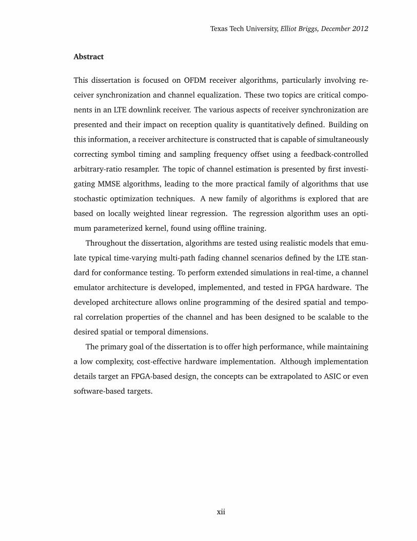
Abstract
This dissertation is focused on OFDM receiver algorithms, particularly involving re-
ceiver synchronization and channel equalization. These two topics are critical compo-
nents in an LTE downlink receiver. The various aspects of receiver synchronization are
presented and their impact on reception quality is quantitatively defined. Building on
this information, a receiver architecture is constructed that is capable of simultaneously
correcting symbol timing and sampling frequency offset using a feedback-controlled
arbitrary-ratio resampler. The topic of channel estimation is presented by first investi-
gating MMSE algorithms, leading to the more practical family of algorithms that use
stochastic optimization techniques. A new family of algorithms is explored that are
based on locally weighted linear regression. The regression algorithm uses an opti-
mum parameterized kernel, found using offline training.
Throughout the dissertation, algorithms are tested using realistic models that emu-
late typical time-varying multi-path fading channel scenarios defined by the LTE stan-
dard for conformance testing. To perform extended simulations in real-time, a channel
emulator architecture is developed, implemented, and tested in FPGA hardware. The
developed architecture allows online programming of the desired spatial and tempo-
ral correlation properties of the channel and has been designed to be scalable to the
desired spatial or temporal dimensions.
The primary goal of the dissertation is to offer high performance, while maintaining
a low complexity, cost-effective hardware implementation. Although implementation
details target an FPGA-based design, the concepts can be extrapolated to ASIC or even
software-based targets.
xii

Texas Tech University, Elliot Briggs, December 2012
1 Preface
1.1 Background
I was first introduced to DSP in 2005 when I took the course at Texas Tech, instructed by
my committee co-chair Dr. Karp. At that point in time, I was already very enthusiastic
about communication circuit design. Later, I signed up for “Modern Communications
Circuits” instructed by Dr. Nutter, my commitee chair, who presented the concept of
software defined radio at the end of the course. I was intrigued. I later became a
graduate student studying embedded systems under Dr. Nutter, who sent me away
for a 6 month internship at Innovative Integration in Simi Valley, California. This is
where the bits and pieces of interesting topics reached critical mass. At Innovative, I
was introduced to FPGAs, spending most of my time learning how to implement DSP
algorithms that run in real-time for customers’ software-defined radio projects. The
connect between DSP, FPGAs and communications convinced me that I wasn’t done
being a graduate student.
After a few months back at Texas Tech, I submitted a proposal to Dan McLane at
Innovative to build an OFDM receiver in an FPGA, a project I thought would be chal-
lenging enough to last at least a semester or two. He had heard about this new “LTE”
standard that seemed to be attracting the attention of many of his customers. Much
of the work in this dissertation is a result of this project. FPGA implementation was
paramount throughout the work with Innovative. Together, we developed and imple-
mented an LTE receiver and a real-time wireless channel emulator. During this work,
I became a firm believer of the “design for implementation” philosophy. The central
theme of this dissertation is not only the various algorithms, but their implementation
in a real-time system.
1.2 Acknowledgments
The biggest gratitude is to my wife, Kristin. Together, I believe we clearly demonstrate
the “better than the sum of the pieces” concept. I’d like to thank her for her tolerance
with my textbook addiction, especially while on vacation. I also owe a huge debt of
gratitude to my committee chairs, Drs. Tanja Karp and Brian Nutter, who have with-
stood the inhumane job of reading my papers and answering my questions. My com-
mittee chairs have both given me great inspiration and have illustrated an impossibly
high standard that I will always strive to reach. I’d also like to thank Dan McLane, the
former co-founder and vice president at Innovative Integration. Without Dan’s support,
1
Texas Tech University, Elliot Briggs, December 2012
I may have never reached the “critical mass” moment that I mentioned. I’d also like
to thank my colleagues with whom I worked at Innovative, Amit Mane and Chunmei
Kang.
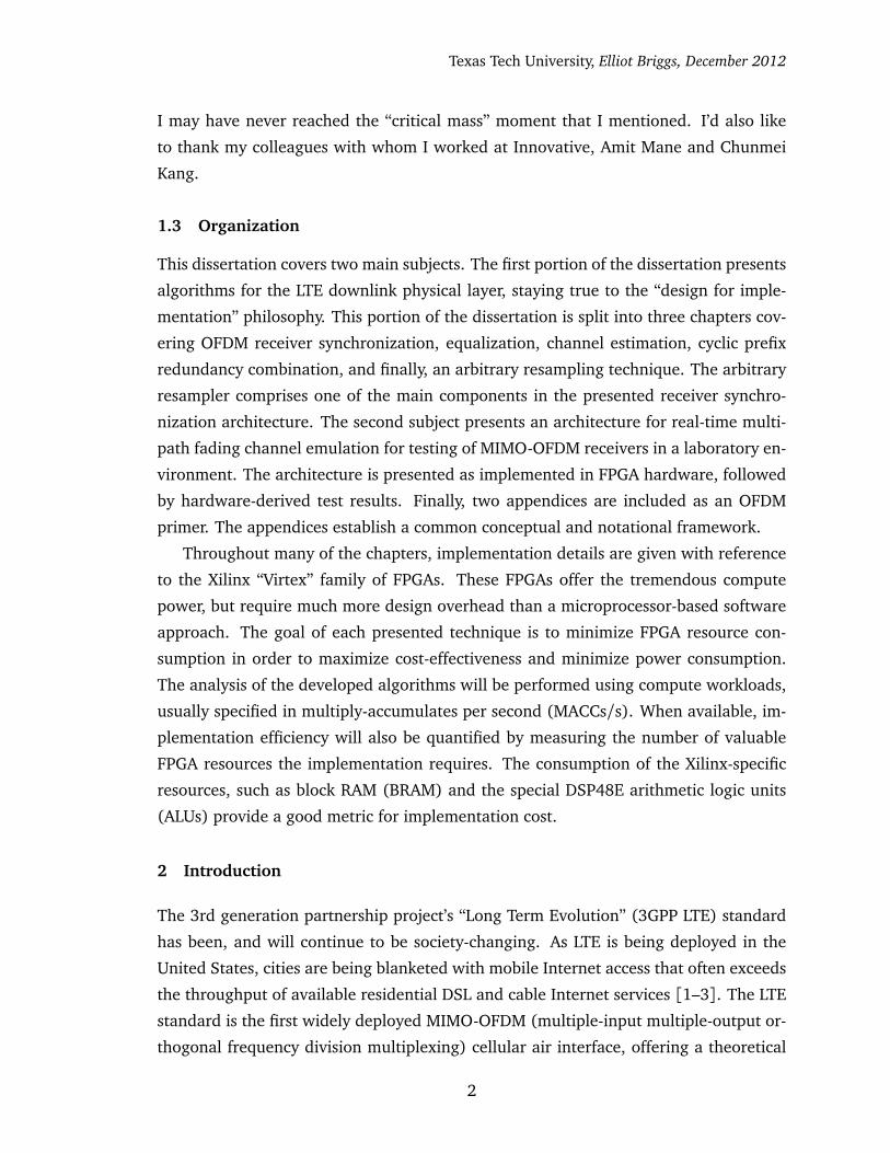
1.3 Organization
This dissertation covers two main subjects. The first portion of the dissertation presents
algorithms for the LTE downlink physical layer, staying true to the “design for imple-
mentation” philosophy. This portion of the dissertation is split into three chapters cov-
ering OFDM receiver synchronization, equalization, channel estimation, cyclic prefix
redundancy combination, and finally, an arbitrary resampling technique. The arbitrary
resampler comprises one of the main components in the presented receiver synchro-
nization architecture. The second subject presents an architecture for real-time multi-
path fading channel emulation for testing of MIMO-OFDM receivers in a laboratory en-
vironment. The architecture is presented as implemented in FPGA hardware, followed
by hardware-derived test results. Finally, two appendices are included as an OFDM
primer. The appendices establish a common conceptual and notational framework.
Throughout many of the chapters, implementation details are given with reference
to the Xilinx “Virtex” family of FPGAs. These FPGAs offer the tremendous compute
power, but require much more design overhead than a microprocessor-based software
approach. The goal of each presented technique is to minimize FPGA resource con-
sumption in order to maximize cost-effectiveness and minimize power consumption.
The analysis of the developed algorithms will be performed using compute workloads,
usually specified in multiply-accumulates per second (MACCs/s). When available, im-
plementation efficiency will also be quantified by measuring the number of valuable
FPGA resources the implementation requires. The consumption of the Xilinx-specific
resources, such as block RAM (BRAM) and the special DSP48E arithmetic logic units
(ALUs) provide a good metric for implementation cost.
2 Introduction
The 3rd generation partnership project’s “Long Term Evolution” (3GPP LTE) standard
has been, and will continue to be society-changing. As LTE is being deployed in the
United States, cities are being blanketed with mobile Internet access that often exceeds
the throughput of available residential DSL and cable Internet services [1–3]. The LTE
standard is the first widely deployed MIMO-OFDM (multiple-input multiple-output or-
thogonal frequency division multiplexing) cellular air interface, offering a theoretical
2
Texas Tech University, Elliot Briggs, December 2012
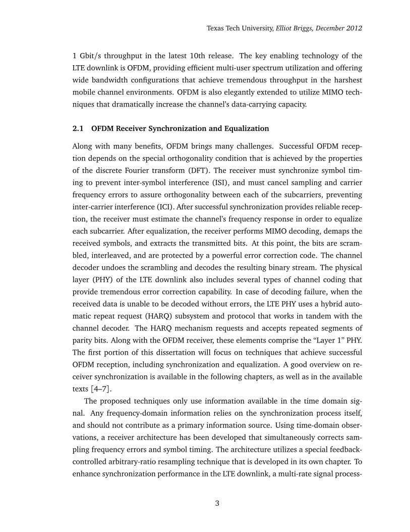
1 Gbit/s throughput in the latest 10th release. The key enabling technology of the
LTE downlink is OFDM, providing efficient multi-user spectrum utilization and offering
wide bandwidth configurations that achieve tremendous throughput in the harshest
mobile channel environments. OFDM is also elegantly extended to utilize MIMO tech-
niques that dramatically increase the channel’s data-carrying capacity.
2.1 OFDM Receiver Synchronization and Equalization
Along with many benefits, OFDM brings many challenges. Successful OFDM recep-
tion depends on the special orthogonality condition that is achieved by the properties
of the discrete Fourier transform (DFT). The receiver must synchronize symbol tim-
ing to prevent inter-symbol interference (ISI), and must cancel sampling and carrier
frequency errors to assure orthogonality between each of the subcarriers, preventing
inter-carrier interference (ICI). After successful synchronization provides reliable recep-
tion, the receiver must estimate the channel’s frequency response in order to equalize
each subcarrier. After equalization, the receiver performs MIMO decoding, demaps the
received symbols, and extracts the transmitted bits. At this point, the bits are scram-
bled, interleaved, and are protected by a powerful error correction code. The channel
decoder undoes the scrambling and decodes the resulting binary stream. The physical
layer (PHY) of the LTE downlink also includes several types of channel coding that
provide tremendous error correction capability. In case of decoding failure, when the
received data is unable to be decoded without errors, the LTE PHY uses a hybrid auto-
matic repeat request (HARQ) subsystem and protocol that works in tandem with the
channel decoder. The HARQ mechanism requests and accepts repeated segments of
parity bits. Along with the OFDM receiver, these elements comprise the “Layer 1” PHY.
The first portion of this dissertation will focus on techniques that achieve successful
OFDM reception, including synchronization and equalization. A good overview on re-
ceiver synchronization is available in the following chapters, as well as in the available
texts [4–7].
The proposed techniques only use information available in the time domain sig-
nal. Any frequency-domain information relies on the synchronization process itself,
and should not contribute as a primary information source. Using time-domain obser-
vations, a receiver architecture has been developed that simultaneously corrects sam-
pling frequency errors and symbol timing. The architecture utilizes a special feedback-
controlled arbitrary-ratio resampling technique that is developed in its own chapter. To
enhance synchronization performance in the LTE downlink, a multi-rate signal process-
3
Texas Tech University, Elliot Briggs, December 2012
ing technique has been developed that is able to detect the LTE primary synchroniza-
tion signal in a computationally efficient manner. The computational workload as well
as the implementation aspects are compared between the developed technique and a
more traditional approach.
Next, a framework for adaptive channel equalization is presented that entirely by-
passes the need to perform channel estimation. The technique acknowledges that the
second-order statistics of the channel’s frequency response are unlikely to be explic-
itly known by the receiver, unlike many other publications on the topic. The adaptive
equalization methods approach the minimum mean-squared error (MMSE) solution.
Other optimal channel estimation algorithms can be derived using a regression-based
approach. Using a pre-defined model for the data, an optimal filter can be derived
in a similar manner as the MMSE methods using quadratic optimization to minimize
error. In an attempt to provide optimality over a variety of conditions, a parameterized
kernel is used and the optimal parameter is found using a developed offline training
technique. Finally, several interpolation techniques are explored to construct the equal-
ization matrix for the remaining subcarrier locations in the frequency-time grid. The
featured interpolation procedure is optimized for minimum latency and memory usage.
2.2 System Architecture for Real-Time Multi-Path Wireless Channel Emulation
As a designer develops an OFDM receiver, performance-measuring simulations must
constantly verify the intended operation. In the first stages of design, verification can
be performed using short computer simulations of realistic scenarios in a software envi-
ronment such as MATLAB. For realism, the simulations can mimic or emulate common
conditions that occur in the intended operating environment using statistical models.
Many industry-standard models have been established for commonly occurring mobile
operating environments. As the developer moves beyond the prototyping phase and
into implementation, simulation tasks become more time-critical. Finally, when the de-
sign is nearly deployed, long-term real-time simulation becomes increasingly integral.
At this stage, a real-time channel emulator is an invaluable tool, allowing the receiver
to operate in a simulated environment in real-time for extended durations of time with-
out encountering repetitive channel conditions. This dissertation presents a real-time
MIMO channel emulator architecture that has been developed and implemented in
FPGA hardware. The architecture allows the user to program the desired temporal and
spatial aspects of the channel, allowing real-time simulation using industry-standard,
as well as custom channel models.
4

Texas Tech University, Elliot Briggs, December 2012
2.3 Cyclic Prefix Redundancy Combination and Arbitrary-Ratio Resampling
Two additional topics are included that provide performance enhancement to OFDM
reception. Cyclic prefix redundancy combination provides a boost in SNR, and the
arbitrary-ratio resampler enables sampling frequency offset correction.
2.3.1 Cyclic Prefix Redundancy Combination with LTE Context
Channels with memory spread the energy of the transmitted OFDM symbols across
time. In an OFDM system, symbol overlap causes harmful inter-symbol interference
(ISI). To protect against ISI, a cyclic extension, or cyclic prefix (CP) of the transmitter’s
IDFT output is performed to provide a sacrificial guard interval. The CP is an elegant
solution that has many attractive properties. The CP is phase-continuous with the sym-
bol, minimizing additional spectral emissions, it provides tolerance to symbol timing
errors, and it circularizes the channel convolution, providing single-tap-per-subcarrier
equalization. By it’s nature, it also provides redundancy in each OFDM symbol. The
segment of the CP that is left uncorrupted by ISI is available as a copy of portion of
the transmitted symbol. If the receiver is aware of the channel’s length, or excess de-
lay, it can select the uncorrupted segment of CP and utilize the available redundancy.
The channels excess delay is readily available in the existing channel estimation com-
ponents in the receiver. Using the knowledge of the channel’s excess delay, a method
is shown that performs this combination at near-zero computational cost to achieve
modest gains in signal-to-noise (SNR) ratio by combining the available redundancy.
2.3.2 Arbitrary-Ratio Resampling Using a Reformulated Farrow Filter
The locally weighted regression algorithm shows a promising alternative to the typical
stochastic optimization class of algorithms when used for channel estimation purposes.
By reformulating the regression algorithm, an optimal filter matrix is found for the
given kernel using the assumption of periodically sampled data. Along with Horner’s
rule, the filter’s matrix operation arrives at Farrow’s filter structure using an alterna-
tive formulation. Using this approach, the width of the pass-band, along with other
features of the Farrow filter can be “tuned”. When the Farrow filter is prefixed with
an upsampling component, arbitrary-ratio resampling can be performed with attrac-
tive stop-band attenuation properties. This design is utilized in the presented receiver
synchronization architecture and is featured throughout its simulation results.
5
Texas Tech University, Elliot Briggs, December 2012
2.4 Contributions
The significant contributions of this dissertation are summarized by the following list:
• An OFDM receiver architecture that simultaneously estimates and corrects sam-
pling frequency offset and symbol timing in the time domain. The technique is
presented and verified using a generic OFDM system configuration without spe-
cial training symbols or preambles while operating in a multi-path fading channel
with high mobility.
• A multi-rate algorithm for detecting symbol timing and the sector ID using the pri-
mary synchronization signal (PSS) in the LTE downlink. The multi-rate approach
is shown to have many superior properties when compared to the overlap-add
algorithm.
• A machine learning technique for optimal channel estimation. Using locally
weighted linear regression with a parameterized kernel, maximum likelihood es-
timation of the channel’s frequency response can be performed using a constant
filter matrix. A convex optimization technique is then used to approximate the
MMSE kernel parameter.
• The locally weighted linear regression technique formulates the well-known Far-
row filter. Using the parametrized kernel, a variable bandwidth Farrow filter is
created with continuously-variable linear group delay in the passband. Using
Horner’s rule, an efficient implementation structure is realized.
• A simple technique utilizes excess CP to achieve modest gains in SNR, when
provided knowledge of the channel’s excess delay. The redundancy combination
correlates the noise across frequency. The correlation relationship is explicitly
derived.
• An architecture is developed that implements an industry-standard model for
emulating spatiotemporally correlated multi-path fading channels in FPGA hard-
ware, operating in real-time, capable of processing modern wide-bandwidth sig-
nals.
6
Texas Tech University, Elliot Briggs, December 2012
3 OFDM Receiver Synchronization
Synchronization is perhaps the most performance-influencing component in an OFDM
receiver. Without reliable synchronization, the fundamental orthogonality property of
OFDM given by the DFT is lost. To ensure orthogonal operation, a wireless receiver
must perform the delicate balancing act of timinig, frequency, and sample clock syn-
chronization, each of which must be estimated using only the received signal. Often-
times a “chicken and the egg” situation arises. Without timing synchronization, can the
receiver estimate the sample clock frequency error? With a sampling frequency error,
can the receiver estimate and perform timing synchronization? In the normal case, the
receiver comes online with all three of these inter-dependent synchronization tasks to
perform.
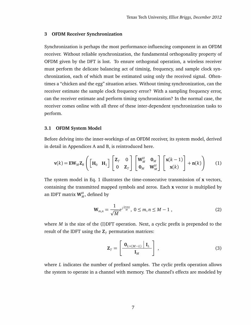
3.1 OFDM System Model
Before delving into the inner-workings of an OFDM receiver, its system model, derived
in detail in Appendices A and B, is reintroduced here.
v(k) = EWMZR
h
H0 H1
i
ZT 0
0 ZT
WHM 0M
0M WHM
x(k− 1)
x(k)
+ n(k)
!
(1)
The system model in Eq. 1 illustrates the time-consecutive transmission of x vectors,
containing the transmitted mapped symbols and zeros. Each x vector is multiplied by
an IDFT matrix WHM , defined by
Wm,n =1p
Me j 2πmn
M , 0≤ m, n≤ M − 1 , (2)
where M is the size of the (I)DFT operation. Next, a cyclic prefix is prepended to the
result of the IDFT using the ZT permutation matrices:
ZT =
0L×(M−L) IL
IM
, (3)
where L indicates the number of prefixed samples. The cyclic prefix operation allows
the system to operate in a channel with memory. The channel’s effects are modeled by
7

Texas Tech University, Elliot Briggs, December 2012
the block matrix multiplication with H0 and H1
H0 =
0 · · · hd · · · h2...
. . . . . ....
.... . . hd
.... . .
...
0 · · · · · · · · · 0
H1 =
h1 0 · · · · · · 0...
. . . . . ....
hd · · · h1. . .
.... . . . . . 0
0 hd · · · h1
,
(4)
and the addition of the WGN vector n. After the channel has had its influence on the
signal, the receiver selects the appropriate block of samples for its DFT operation using
the ZR permutation matrix
ZR =h
0M×L IM
i
. (5)
The vector of selected samples is then multiplied by the DFT matrix, resulting in a
vector of symbols that have been affected by the channel’s frequency response. The
E matrix is used to equalize the channel’s effects, allowing for demapping and the ex-
traction of the transmitted data. In this model, the receiver is responsible for selecting
the block of samples for each symbol and equalizing the channel’s effects. These op-
erations will be two of the main receiver functions discussed in the following sections
and chapters.
3.2 Timing Synchronization
In an ideal OFDM system, as shown in Fig. 82, the serial-to-parallel and parallel-to-
serial components operate in perfect synchronization. If the perfect synchronization
assumption is removed, which is the case with all realizable wireless OFDM commu-
nications systems, the receiver operates on a time-shifted version of the transmitted
signal. A general description of the effect of timing offset in an OFDM system can be
used when the sampling clocks of the transmitter and receiver are perfectly matched
in frequency, but the sampling clock phases are not guaranteed to be aligned, causing
a constant fractional timing offset. For completeness, the phase offset between the
8
Texas Tech University, Elliot Briggs, December 2012
sampling clocks can extend beyond 2π so that modeled delays may extend beyond the
integer sample duration. The continuous-valued timing offset causes a phase shift in
the frequency domain according to
φ = e− j2πτk
M
k = (0, 1, · · · , M − 1)−M
2,
τ ∈ [0,M
2) ,
(6)
where M is the size of the DFT matrix WM in the OFDM system and τ is the continuous
delay that represents the timing offset between the transmitter and receiver in units of
samples.
To model fractional timing offset in simulation, when the system typically has per-
fectly synchronous sampling phase (i.e. when using MATLAB, Simulink, or other syn-
chronous mathematical descriptions of a wireless system), a simple FIR filter is able
to model the effects of fractional timing offset by linearly shifting the phase with fre-
quency.
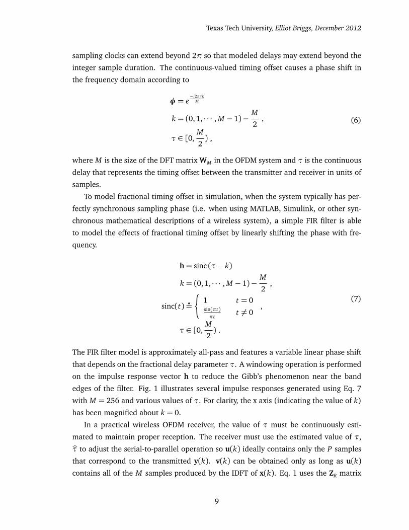
h= sinc (τ− k)
k = (0,1, · · · , M − 1)−M
2,
sinc(t)¬
(
1 t = 0sin(πt)πt
t 6= 0,
τ ∈ [0,M
2) .
(7)
The FIR filter model is approximately all-pass and features a variable linear phase shift
that depends on the fractional delay parameter τ. A windowing operation is performed
on the impulse response vector h to reduce the Gibb’s phenomenon near the band
edges of the filter. Fig. 1 illustrates several impulse responses generated using Eq. 7
with M = 256 and various values of τ. For clarity, the x axis (indicating the value of k)
has been magnified about k = 0.
In a practical wireless OFDM receiver, the value of τ must be continuously esti-
mated to maintain proper reception. The receiver must use the estimated value of τ,
bτ to adjust the serial-to-parallel operation so u(k) ideally contains only the P samples
that correspond to the transmitted y(k). v(k) can be obtained only as long as u(k)
contains all of the M samples produced by the IDFT of x(k). Eq. 1 uses the ZR matrix
9

Texas Tech University, Elliot Briggs, December 2012
−20 −15 −10 −5 0 5 10 15 20
0
0.5
1
Fractional Timing Offset Model − Channel Impulse Response
τ=−0.5
−20 −15 −10 −5 0 5 10 15 20
0
0.5
1
τ=−0.3
−20 −15 −10 −5 0 5 10 15 20
0
0.5
1
τ=−0.1
−20 −15 −10 −5 0 5 10 15 20
0
0.5
1
τ=0.1
−20 −15 −10 −5 0 5 10 15 20
0
0.5
1
τ=0.3
−20 −15 −10 −5 0 5 10 15 20
0
0.5
1
τ=0.5
relative time index k
Figure 1: FIR Filter That Models the Effects of Fractional Timing Error (M = 256)
to select the final block of M samples in each symbol. To keep this notation, it will
be assumed that the serial-to-parallel operation eliminates the integer portion of the
delay τint = floor(τ), leaving only the fractional delay τfrac = τ − τint. In the likely
case where 0 < τfrac < 1, the fractional delay can be lumped into channel’s impulse
response. Recalling Eq. 162, the channel’s effects are modeled using two horizontally
concactenated matrices, H0 and H1, each generated using the channel’s impulse re-
sponse vector h, which has d elements. The interpolated channel impulse response
that lumps the channel’s impulse response with the fractional delay effects can be de-
10
Texas Tech University, Elliot Briggs, December 2012
m=0
m < -(L-d) (left error)
m > 0 (right error)
CP CPd
Figure 2: Illustration of “Left” and “Right” Symbol Timing Error Positions
fined by the vector g.
g=d∑
n=1
hnsinc(τfrac+ (n− 1)− k) ,
k = 0,1, . . . , M − 1
(8)
Again, the sinc in Eq. 8 requires the use of a windowing operation to reduce the Gibb’s
phenomenon near the band edges. When the channel is not the unit impulse, the
receiver cannot distinguish the effect of the channel vs. fractional timing error [8].
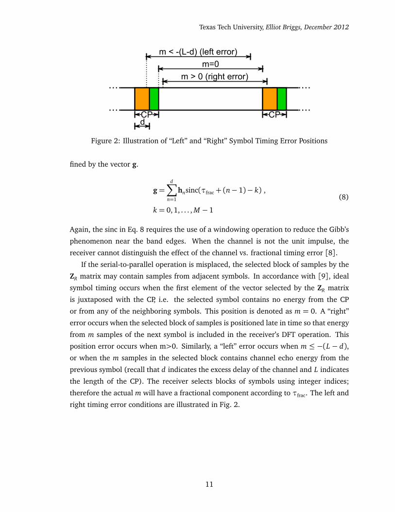
If the serial-to-parallel operation is misplaced, the selected block of samples by the
ZR matrix may contain samples from adjacent symbols. In accordance with [9], ideal
symbol timing occurs when the first element of the vector selected by the ZR matrix
is juxtaposed with the CP, i.e. the selected symbol contains no energy from the CP
or from any of the neighboring symbols. This position is denoted as m = 0. A “right”
error occurs when the selected block of samples is positioned late in time so that energy
from m samples of the next symbol is included in the receiver’s DFT operation. This
position error occurs when m>0. Similarly, a “left” error occurs when m ≤ −(L − d),
or when the m samples in the selected block contains channel echo energy from the
previous symbol (recall that d indicates the excess delay of the channel and L indicates
the length of the CP). The receiver selects blocks of symbols using integer indices;
therefore the actual m will have a fractional component according to τfrac. The left and
right timing error conditions are illustrated in Fig. 2.
11

Texas Tech University, Elliot Briggs, December 2012
The level of interference caused by the two types of symbol timing errors is not
symmetric, i.e. the level of interference caused by a left error is not equal to a right
error, given the same absolute offset. The signal-to-interference ratio (SIR) of a right
error is defined by [9]
SIRr =(M −m)2
(2M −m)m− 2 M−mσ2
H
∑m−1k=0
∑dk′=k+2σ
2hk′
,
m> 0
(9)
where the channel gain σ2H = hHh and the scalar σ2
hk′= h∗k′hk′ is the power of a given
channel tap at index k′. Similarly, the SIR for the left error is defined by
SIRl =(M − c)2
(2M − c) c− 2 M−cσ2
H
∑c−1k=0
∑L+c+kk′=k+1σ
2hk′
,
c = d − (L+m) ,
−L ≤ m≤ (−L+ d − 1)
(10)
The example shown in [9] defines the channel vector h= [0.3484, 0.3910,0, 0,0.4386,
0.3910,0, 0.3405,0.3106, 0.2767,0.2467, 0.1746], L = 52 and M = 512. Using the
specified channel vector, Fig. 3, reproduced from [9], shows that the level of interfer-
ence introduced by left and right errors is not equal, which can be intuitively justified.
The channel’s impulse response usually contains more energy in the elements with the
least amount of relative delay, thus for a left error, the ISI energy is initially less than
for the right error, given the same absolute error. With a left error, the desired symbol’s
energy tends to outweigh the interference in the erroneously selected portion of the CP.
In a right error, the samples erroneously selected from the next symbol contain chan-
nel echoes of the desired symbol, which aren’t useful for demodulation, and the next
symbol’s energy.
The symbol timing in a wireless receiver must be estimated using only the in-
formation in the received signal. Many symbol timing estimators exist that provide
good performance, however noise and channel conditions can affect estimation preci-
sion [10–13].
The integer portion bτint of the offset estimate bτ is used to adjust the serial-to-parallel
operation so only the estimated fractional timing offset bτfract remains. The estimation
error can be modeled by considering the symbol timing estimates to be a random vari-
able denoted by bτ(t) and its instantaneous realization bτ.
12

Texas Tech University, Elliot Briggs, December 2012
−60 −40 −20 0 20 40 6010
0
101
102
103
104
SIR
m
SIR vs. Integer Symbol Timing Position m
SIR for Left Errors
SIR for Right Errors
Figure 3: SIR vs. Symbol Timing Error m - Left and Right Errors
The effect of a timing error can be observed by assuming that bτ(t) is normally
distributed with a time-invariant mean τ and variance σ2τ. The maximum-likelihood
estimates of τ and σ2τ given N realizations of bτ(t) are µ
bτ(t) and σ2bτ(t), realized by
computing the mean and unbiased variance of the N realizations of bτ(t). For finite N ,
µbτ(t) is denoted as a random variable with a Student’s t-distribution, defined by the
degrees of freedom ν = N − 1. Assuming a finite N , the value of N must be chosen so
timing position estimates are obtained by the receiver in a timely manner (and so that
the receiver can track non-stationary statistics, if present), and so the variations among
realizations of µbτ(t) are small enough such that the probability of erroneous symbol
placement is minimized.
As N → ∞, µbτ → τ, and Var
�
µbτ
�
= bσ2bτ→ 0, therefore bσ2
bτ> 0 for finite N . The
non-zero variance requires careful consideration of the timing window placement. If
the timing window is misplaced by a single sample, a right error can occur (Fig. 3),
therefore the statistical confidence in each realization of µbτ(t) must be analyzed so the
decision of the integer symbol timing position can be given a statistical justification.
Because only integer symbol timing positions can be implemented by choosing an in-
teger number of samples for each DFT operation, the rounding decision policy must be
considered when deciding N . In the following analysis, assume that the timing position
13

Texas Tech University, Elliot Briggs, December 2012
used for the receiver’s serial-to-parallel operation is determined by nearest(µbτ), which
rounds µbτ to the nearest integer.
Using the Student’s t-distribution, the estimated parameters µbτ and σ2
bτcan be used
to determine P(τ ≤ µbτ + z), or the probability that the true timing position estimated
by µbτ is less than the value determined by the offset value z, which defines the prob-
ability threshold offset from the estimated mean, or “critical value”. The value of z is
determined using a pre-defined level of probability denoted by α, such that
P(τ≤ µbτ+ z) = α . (11)
In this analysis, α is constant and the critical value z will be computed according to
the gathered statistics. The remaining task is to define an acceptable value of α and to
compute the value of z, which can be computed using
z = tcdf (α,ν)Se , (12)
where tcdf (α,ν) computes the solution to the inverse Student’s t cumulative-distribution
function (cdf) integral F−1 (α,ν), and the standard error Se is defined by
Se =σbτpN
. (13)
Given the severity of the interference caused by timing errors, and the desire for
smaller averaging windows for more responsive receiver aquisition and tracking, it
may be desirable to implement symbol “timing backoff”, offsetting the symbol position
from the estimated value of τ to assure safe symbol timing placement (reducing the
probability of error). To illustrate the usefulness (necessity) of timing backoff, suppose
a sliding window of N symbol timing estimates are used to generate the symbolwise
time series of estimates µbτ [n] and σ
bτ [n]. The estimates of τ can be recursively com-
puted using
s [n] = s [n− 1] + bτ [n]− bτ [n− N]
µbτ [n] =
s [n]N
,(14)
14

Texas Tech University, Elliot Briggs, December 2012
Similarly, the unbiased variance and standard deviation can be recursively computed
q [n] = bτ [n]2
v [n] = v [n− 1] + q [n]− q [n− N]
σ2bτ [n] =
N v [n]− s [n]2
N (N − 1)
(15)
Note that Eq. 14 and 15 are both computed using an equally weighted (across time)
sliding window of N realizations of bτ(t), each requiring a memory buffer of size N . The
stochastic optimization algorithms presented in [14,15], frequently include techniques
that employ a “forgetting factor” λ to estimate parameters (statistics) that cannot be
assumed to be stationary. These iterative algorithms are attractive as they only require
a single-element memory buffer and are capable of implementing a variable-length av-
eraging window by adjusting the λ parameter. Each recursion applies an exponentially
diminishing weight to older or more “stale” realizations of the statistical parameter to
be estimated. Using this concept, the mean µbτ [n] can be recursively estimated using
µbτ [n] = λµbτ [n− 1] + (1−λ) bτ [n] , (16)
and similarly for bσbτ [n]
σ2bτ [n] = λσbτ [n− 1] + (1−λ)
�
bτ [n]−µbτ [n]
�2 ,
σbτ [n] =
Æ
σ2bτ[n]
(17)
By selecting a forgetting factor λ = 1− 1N
, the equally weighted, or “rectangular” win-
dow recursion and the “decaying” or “forgetting” window recursions can be compared.
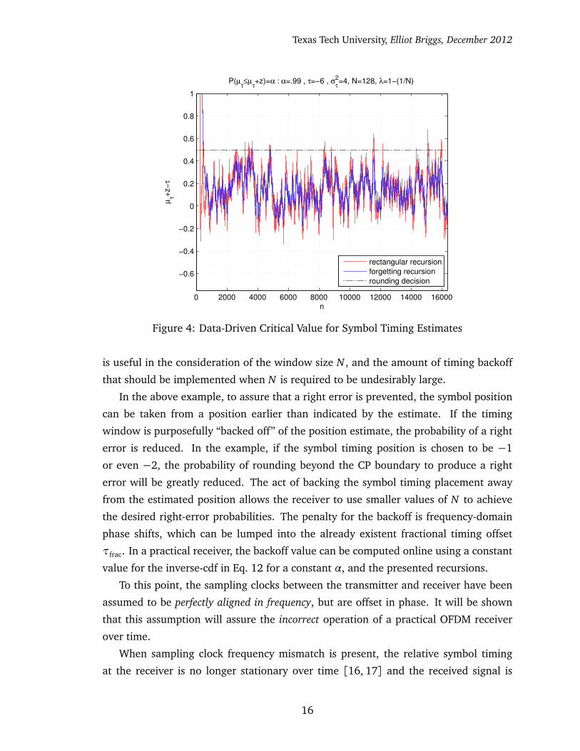
Fig. 4 demonstrates the confidence boundary z for α= .99 on a set of symbol timing
estimates with τ = 0, variance σ2τ = 4, and a sliding window size of N = 128. The red
curve (rectangular window recursion) indicates the true confidence boundary estimates
generated using Eq. 14 and 15 and the definition of the probability in Eq. 11. The blue
curve (forgetting recursion) indicates the confidence boundaries generated from the
approximated values of µbτ [n] and σ
bτ [n] using Eq. 16 and Eq. 17 In this example, the
symbol position τ= 0 corresponds to m= 0, and from Fig. 4, over realizations of bτ(t),
there are often situations where the probability of the timing estimate being below the
decision boundary for the rounding policy µbτ is less than .99, which after the rounding
process, the estimated probability of producing a right error exceeds .01, or more than
1 out of 100 symbols are likely to contain interference from a right error. This analysis
15
Texas Tech University, Elliot Briggs, December 2012
0 2000 4000 6000 8000 10000 12000 14000 16000
−0.6
−0.4
−0.2
0
0.2
0.4
0.6
0.8
1
P(µτ≤µ
τ+z)=α : α=.99 , τ=−6 , σ
2
τ=4, N=128, λ=1−(1/N)
µτ+
z−
τ
n
rectangular recursion
forgetting recursion
rounding decision
Figure 4: Data-Driven Critical Value for Symbol Timing Estimates
is useful in the consideration of the window size N , and the amount of timing backoff
that should be implemented when N is required to be undesirably large.
In the above example, to assure that a right error is prevented, the symbol position
can be taken from a position earlier than indicated by the estimate. If the timing
window is purposefully “backed off” of the position estimate, the probability of a right
error is reduced. In the example, if the symbol timing position is chosen to be −1
or even −2, the probability of rounding beyond the CP boundary to produce a right
error will be greatly reduced. The act of backing the symbol timing placement away
from the estimated position allows the receiver to use smaller values of N to achieve
the desired right-error probabilities. The penalty for the backoff is frequency-domain
phase shifts, which can be lumped into the already existent fractional timing offset
τfrac. In a practical receiver, the backoff value can be computed online using a constant
value for the inverse-cdf in Eq. 12 for a constant α, and the presented recursions.
To this point, the sampling clocks between the transmitter and receiver have been
assumed to be perfectly aligned in frequency, but are offset in phase. It will be shown
that this assumption will assure the incorrect operation of a practical OFDM receiver
over time.
When sampling clock frequency mismatch is present, the relative symbol timing
at the receiver is no longer stationary over time [16, 17] and the received signal is
16
Texas Tech University, Elliot Briggs, December 2012
degraded by inter-carrier interference (ICI) [18]. In a system with sample clock offset
(SCO), the symbol timing has two parameters, the drift rate∆τ and the current symbol
timing position τ. The drift rate ∆τ will be denoted in units of samples per symbol,
that is, the timing shift in unit-sample durations that occur over the unit-time of a
single OFDM symbol duration. The sample clock offset ∆ fSCO between the transmitter
and receiver is defined by
∆ fSCO = fT X − fRX , (18)
where fT X and fRX define the transmitter and receiver sampling clock frequencies, re-
spectively and ∆ fSCO is denoted in units of Hz, or alternatively, in samples per second.
The sampling clock error effectively resamples the transmitted signal. Suppose the
sample clock error between the transmitter and receiver is∆ fSCO = (−)+100 Hz, caus-
ing, 100 (fewer) additional samples to be (removed from) added to the ideal received
signal each second. Given an ideal ideal number of transmitted samples per symbol P
(Eq. 166), and a transmitter sampling rate fT X , the transmitted symbol rate is defined
by
fT Xs ym =fT X
P, (19)
with units of symbols per second. The constant timing window drift ∆τ is now defined
by
∆τ=∆ fSCO
fT Xs ym(20)
with units of samples per symbol. The timing window drift is a symptom of sample
clock offset that is detectable using nothing but the time series of successive symbol
timing estimates. The drift parameter ∆τ contains both the magnitude and direction
information that allows the SCO to be directly estimated.
Ideally, the symbol timing positions are determined by
δτ [n] = δτ [n− 1] +∆τ
τ [n] = δτ [n] ,(21)
However, to model random estimation error, the zero-mean random variable s(t) with
variance σ2s is included.
δτ [n] = δτ [n− 1] +∆τ
bτ [n] = δτ [n] + s [n] ,(22)
bτ [n]must be realized for each received OFDM symbol to maintain the proper samples-
17

Texas Tech University, Elliot Briggs, December 2012
per-symbol units used for ∆τ. The instantaneous measurement of the SCO can be
obtained using Eq. 22 in Eq. 23.
∆τ [n] = δτ [n]−δτ [n− 1]
Óδτ [n] = bτ [n]
Óδτ [n− 1] = bτ [n− 1]
(23)
therefore
d∆τ [n] = bτ [n]− bτ [n− 1] (24)
with the variance
Var�
d∆τ [n]�
= 2σ2s (25)
Note that 0 < |∆τ| << 1 for “normal” levels of SCO and the symbol timing esti-
mates are usually indicated by integers, requiring a large number of ∆τ estimates to
achieve sufficient precision. A moving average of SCO measurements can be obtained
using a recursive estimation algorithm (Eq. 16). However, the SCO measurement will
not need to be directly measured, but will be used as a control variable for the receiver
to actively cancel SCO using an arbitrary resampling component. More details on this
will be presented in the next section.
3.3 Sampling Clock Frequency Offset and Symbol Timing Correction: A Joint
Effort
Each aspect of synchronization in an OFDM receiver is closely and oftentimes inter-
related. Such is the case between symbol timing and SCO. Symbol timing drift is
a symptom caused by the resampling process from the SCO. In this case, it is more
worthwhile to treat the disease that causes the symptom, rather than just treating the
symptom and ignoring the root cause. SCO produces other symptoms, most of which
are from the effect of the drifting timing window.
As the symbol timing drifts, the fractional component τfrac is continuously varied. If
the receiver is capable of tracking the integer timing offset component τint, frequency
domain phase-shifts introduced by τfrac are still present. In the conditions of a time-
invariant channel, it is possible, although not advisable to measure SCO in the fre-
quency domain. If the channel is time-varying, the receiver cannot be expected to
18
Texas Tech University, Elliot Briggs, December 2012
1 200 400 600 800 1000 12000
2
4
6
8
10
12
14
16
18
subcarrier index
degra
dation (
dB
)
SNR Degradation vs. Subcarrier Index at Es/No = 50 dB
1 ppm
5 ppm
10 ppm
20 ppm
Figure 5: SNR Degradation vs. Subcarrier Index
distinguish between the varying phase shift caused by SCO and the constantly chang-
ing frequency response of the channel [8]. The time-varying frequency domain phase
shifts indirectly resulting from SCO are a symptom of a symptom of the SCO. Addition-
ally, to measure SCO in the frequency domain, the receiver is assumed to have achieved
sufficient symbol timing synchronization to produce frequency-domain symbols with-
out ISI from timing errors and inter-carrier interference (ICI) from other sources. If
SCO is present, the resampling operation caused by the SCO degrades (destroys) the
orthogonality of the received subcarriers (orthogonality is an absolute term) [18], thus
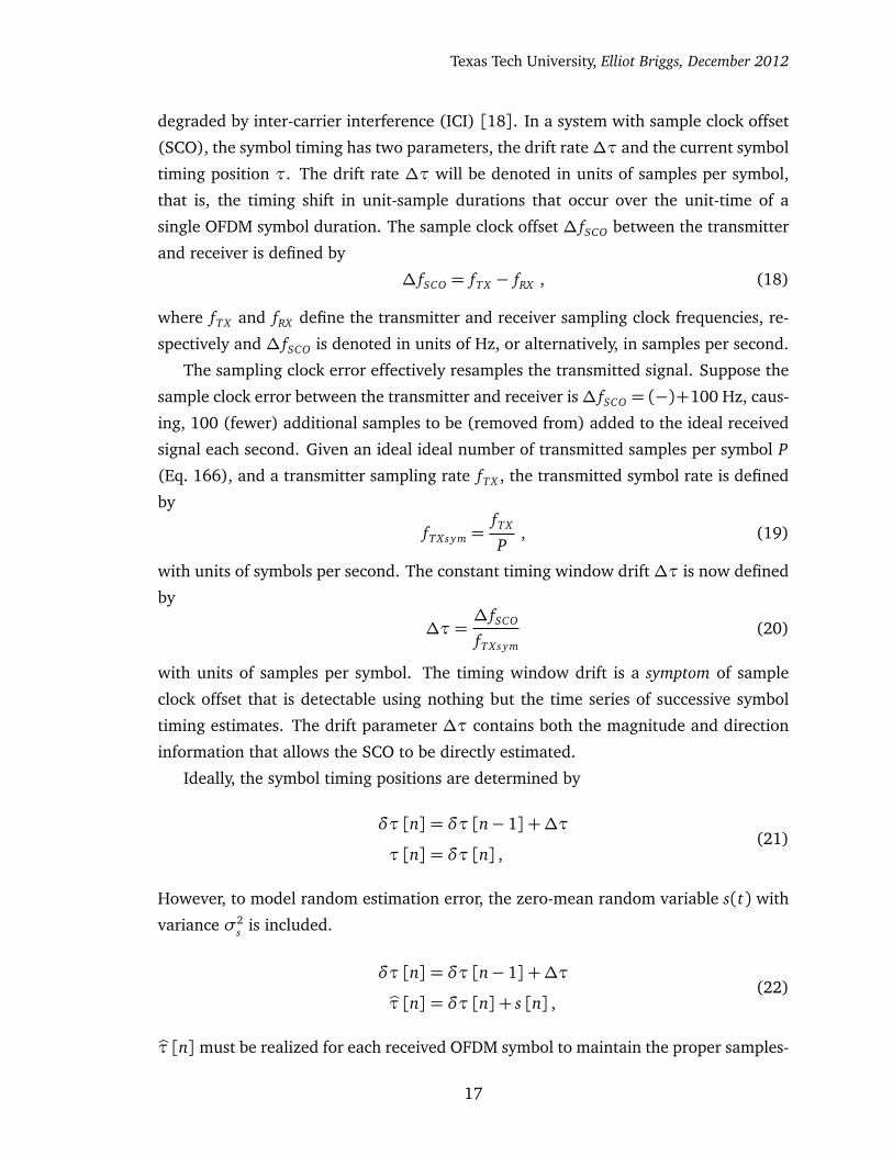
frequency domain measurements are inherently polluted with ICI.
SCO introduces ICI caused by the mislocation of the DFT bin positions in the fre-
quency domain. The amount of ICI on each subcarrier depends on its absolute distance
from the central (DC) subcarrier. The index-dependent degradation of SNR is defined
by
Dn = 10 log10
�
1+1
3
Es
No
�
πn∆ fSCO
fs
�2�
,
n ∈�
−M
2,−
M
2+ 1, . . . ,
M
2− 1�
(26)
where Es and No are the expected symbol energy and noise energy density, respectively
fs indicates the nominal sampling frequency of the system, and n denotes the subcar-
rier, or DFT bin index [18]. Fig. 5 shows the SNR degradation per subcarrier position
19
Texas Tech University, Elliot Briggs, December 2012
5 10 15 20 25 30 35 40
10−1
100
101
102
clock offset (ppm)
de
gra
da
tio
n
SNR Degradation vs. SCO at Varying Es/No (subcarrier index = 1200)
20 dB
30 dB
40 dB
50 dB
Figure 6: SNR Degradation vs. SCO with Varying Es
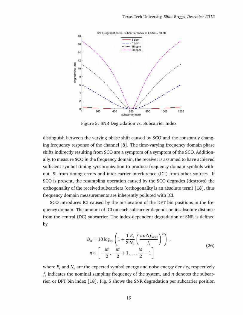
N0
n for several levels of SCO normalized to parts-per-million (ppm) in example OFDM
configuration with 1200 centrally-located subcarriers using a FFT size of M = 2048.
The demonstrated SCO levels, which are quite realistic for low-cost clock oscillators,
show significant SNR degradation. Note that Fig. 5 illustrates the SNR degradation
at a fixed Es
No= 50 dB. Fig. 6 shows the maximum degradation levels located at the
outermost subcarrier indices for several values of Es
No.
Receiver architectures exist that acknowledge the ability to detect SCO in the time-
domain using symbol timing information, yet fail to acknowledge the effects of the SCO
other than phase shifts from fractional symbol timing error [19]. This architecture only
tracks and corrects the phase from the fractional symbol symbol timing errors as the
timing position drifts, leaving the ICI unmitigated. The only component that benefits
from this design is the channel estimator.
The proposed receiver architecture uses the symbol timing information to actively
cancel the SCO by resampling the received signal. The resampling action is performed
using arbitrary-ratio resampler, requiring no additional physical hardware, such as a
phase-locked loop or a voltage-controlled crystal oscillator. After correctly resampling
the received signal, SCO-induced ICI is eliminated, and the symbol timing becomes
stationary. The arbitrary-ratio resampler is controlled using feedback techniques by ob-
serving symbol timing drift and appropriately adjusting the resampling ratio to achieve
stationary symbol timing.
The receiver’s architecture with the SCO cancelling components is shown in Fig. 7.
20

Texas Tech University, Elliot Briggs, December 2012
FFTFarrow-Based
Resampling Filter
Symbol Timing
Estimator
resampled signalreceived signal
recovered TX clock
RX clock demodulatedOFDMsignal
S/P
measured SCO
interpolation postion
Loop Filter
Accumulator
Figure 7: Receiver Architecture Capable of Synchronizing SCO and Symbol Timing
In this receiver, the incoming signal is constantly resampled by the rate indicated by the
output of the loop-filter-controlled accumulator. The loop filter indicates the measured
SCO in units of samples per sample, which is decremented from the value stored in
an accumulator on each incoming sampling clock cycle. The accumulator produces
the sampling indices used by the Farrow-based resampling filter component, which has
been designed in Ch. 5, and is illustrated in Fig. 52 and Fig. 54.
The following simulations illustrate the SCO detection and correction algorithm
on a generalized OFDM system. In this system, no special training symbols are made
available for timing information, and the symbol timing is derived entirely using the
Beek algorithm using the in-built correlation properties of the CP [13]. The example
uses an FFT size of M = 2048, a CP length of L = 512 with 1200 occupied subcarriers
and a sampling rate of 30.72 MHz. Each ppm of SCO adds 30.72 Hz of absolute error,
introducing ±2.56×10⁻³ samples per symbol per ppm, exactly ±1×10⁻⁶ samples per
sample per ppm.
Fig. 8 shows the magnitude of a received OFDM symbol with a -40 ppm SCO error
magnitude alongside the estimated symbol timing indices found by the Beek algorithm.
The simulated SCO levels represent the worst-case error magnitude for two separate
low-cost 20 ppm clock sources at the transmitter and receiver. The outer subcarriers
clearly display large levels of ICI, corresponding with Eq. 26 and Fig. 5. No noise
has been added to the signal in this simulation; all of the SNR degradation is a result
of ICI. The symbol timing is also clearly impacted, drifting nearly 100 samples over
approximately 950 symbols.
Fig. 9 shows the simulation result under the same conditions using the proposed
architecture. In this simulation, the loop filter has been implemented using a simple
integrating controller that adjusts the Farrow resampler’s input accumulator based on
21

Texas Tech University, Elliot Briggs, December 2012
1 256 512 768 1024 1280 1536 1792 20480
0.25
0.5
0.75
1m
ag
nitu
de
subcarrier index (frequency)
Received OFDM Symbol Magnitude Polluted with −40 ppm of SCO
200 400 600 8001180
1190
1200
1210
1220
1230
1240
1250
1260
1270
1280
1290
estim
ate
d s
ym
bo
l tim
ing
po
sitio
n (
sa
mp
les)
OFDM symbol index (time)
Drifting Symbol Timing Estimates
Figure 8: Received OFDM Signal Afflicted with 40 ppm of SCO: Effects on SNR andSymbol Timing
1 256 512 768 1024 1280 1536 1792 20480
0.25
0.5
0.75
1
ma
gn
itu
de
subcarrier index (frequency)
OFDM Symbol Magnitude After Correction: −40 ppm SCO Error
200 400 600 8001255
1260
1265
1270
1275
1280
estim
ate
d s
ym
bo
l tim
ing
po
sitio
n (
sa
mp
les)
OFDM symbol index (time)
Symbol Timing Estimates
100 200 300 400 500 600 700 800 9000
1
2
3
4x 10
−5 SCO Compensation: Control System Response
OFDM symbol index (time)
sa
mp
les/s
am
ple
Accumulator Input
Known SCO Drift Rate
Figure 9: Received OFDM Signal Afflicted with -40 ppm of SCO After Resampling UsingMeasured Timing Drift Rate and Feedback Control Technique
22
Texas Tech University, Elliot Briggs, December 2012
1 256 512 768 1024 1280 1536 1792 20480
0.25
0.5
0.75
1
1.25
1.5
1.75
magnitude
subcarrier index (frequency)
OFDM Symbol Magnitude After Correction: −40 ppm SCO Error
0 500 1000 1500 2000
1180
1190
1200
1210
1220
1230
1240
1250
estim
ate
d s
ym
bol tim
ing p
ositio
n (
sam
ple
s)
OFDM symbol index (time)
Symbol Timing Estimates
0 200 400 600 800 1000 1200 1400 1600 1800 2000−1
0
1
2
3
4
5x 10
−5 SCO Compensation: Control System Response
OFDM symbol index (time)
sam
ple
s/s
am
ple
Accumulator Input
Known SCO Drift Rate
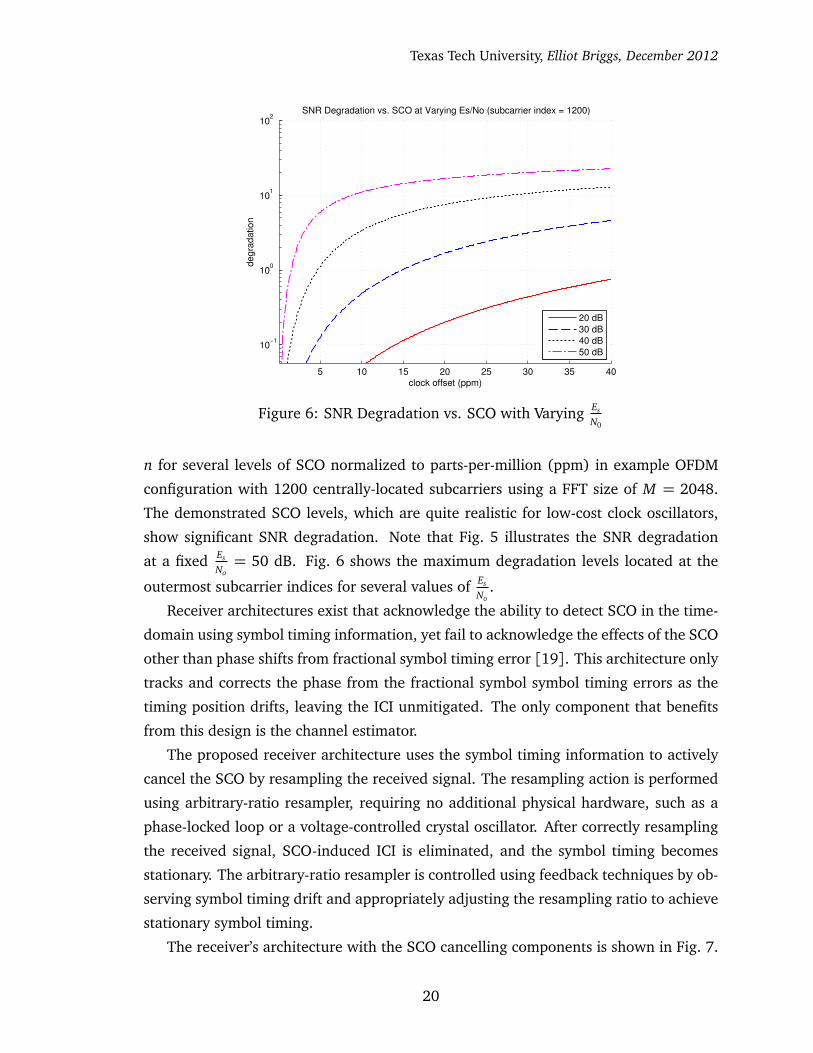
Figure 10: Received OFDM Signal Afflicted with -40 ppm of SCO and EVA-200 ChannelModel: Successful SCO Detection and Correction Using Only Time-Domain Informationin High Mobility Channel Conditions
the observed timing drift. The SCO estimates are generated for each symbol using a
recursively computed moving average over 120 symbols (10 ms), intentionally slow-
ing the response of feedback correction. The symbol magnitude plot in Fig. 9 shows
minimal SNR degradation or distortion from the resampling process after converging
to the ideal resampling ratio. Fig. 9 also verifies that the symbol timing becomes quite
stationary as the SCO compensation converges to the ideal state.
The previous example demonstrates no unique characteristics of either time or fre-
quency domain derived SCO measurement techniques. The simple AWGN channel al-
lows observation of the SCO-induced symbol timing drift in the frequency domain with
minimal ICI in the central subcarrier locations. The next example (Fig. 10) highlights
the unique ability of the proposed method to measure and correct SCO in the midst of
high mobility and multi-path channel conditions. The Beek algorithm continues to be
the only source of symbol timing estimates, which is degraded by the spreading of the
CP’s correlation energy by the multi-path channel, an effect noted by Beek’s original
paper [13]. To counteract the increased estimate variance, a moving average window
is increased to 360 symbols (30 ms) and the loop filter gain is decreased.
23

Texas Tech University, Elliot Briggs, December 2012
The simulation results in Fig. 10 show the same OFDM signal configuration oper-
ating in the LTE-specified extended vehicular A (EVA) model with a 200 Hz maximum
Doppler frequency. The EVA model has 9 channel echoes with a relatively large ex-
cess delay, thus the CP correlation energy is widely distributed, aggressively varying
the symbol timing estimates. The simulation results show the algorithm converged to
nearly cancel the SCO mid-way through the simulation and maintained low steady-
state error despite the large symbol timing estimate variance. The symbol magnitude
subplot in Fig. 10 shows the near-zero ICI in the outer subcarrier locations despite the
severe SCO, mobility, and multi-path conditions.
3.4 Time-Domain Detection of the LTE Primary Synchronization Signal
The previous section highlighted that synchronization of both sampling frequency and
symbol timing can be performed jointly without relying on information from the fre-
quency domain, a particularly attractive property allowing synchronization to be in-
dependent of demodulation reliability. In the LTE downlink, the specially designed
primary synchronization signal (PSS) is at the receiver’s disposal, which is designed to
have optimal correlation properties. Transmitted periodically every 5 ms, the PSS can
greatly enhance nearly every synchronization task in the receiver, including symbol
timing, SCO measurement, carrier frequency offset, and symbol index synchroniza-
tion [20–23].
Unlike the CP, which happens to be correlated with its respective symbol by cir-
cumstance, the LTE PSS is specifically designed to have maximal autocorrelation and
zero cross-correlation with other PSS signals. The CP correlation property is simply an
exploitation arising from the properties of the DFT. It was likely that the CP was never
directly intended to be used for symbol timing synchronization, but to simply provide
an elegant solution to “circularizing” the signal-channel convolution, and to provide a
phase-continuous guard interval to protect against ISI by exploiting the periodic na-
ture of the DFT. Essentially, CP-based timing information is built upon several layers of
exploitations. The goal of this section is not to eliminate the CP as a source of symbol
timing information, but to add another available source. Using the CP as well as the
PSS, overall synchronization performance can be enhanced.
The PSS is generated using Zadoff-Chu (ZC) sequences, which have excellent cyclic
correlation properties. To introduce the generation and properties of generalized ZC
sequences, the analysis in [21, 23] will be followed closely. The ZC sequence zγ [n] is
24

Texas Tech University, Elliot Briggs, December 2012
defined according to
zγ [n] =
(
exp�
− j 2πγN
n(n+2q)2
�
, N even
exp�
− j 2πγN
n(n+1+2q)2
�
, N odd, (27)
where N is the sequence length, n= 0, 1, . . . , N −1, q is an arbitrary integer, and γ is a
positive integer, referred to as the “index”, which is relatively prime to N . In [21, 23],
q = 0 and N is an odd prime. Notice that ZC sequences are always unit-magnitude.
This subtle elegant property allows a ZC sequence to be stored using only the angles of
its elements. The cyclic autocorrelation function of the sequence zγ [n] is
Rzγzγ [m] =N−1∑
n=0
zγ [n] z∗γ [(n+m)mod N] , m= 0, 1, . . . , N − 1 (28)
where Rzγzγ [0] = N and Rzγzγ [m] = 0, for m 6= (0 mod N). Importantly, the cyclic
cross-correlation function of two sequences zγiand zγ j
, both of length N is defined by
Rzγizγ j[m] =
N−1∑
n=0
zγi[n] z∗γ j
[(n+m)mod N] , m= 0,1, . . . , N − 1 . (29)
�
�
�Rzγizγ j
�
�
� = 1/p
N if |n−m| is relatively prime with N , which can be easily satisfied if
N is a prime number, in which case the cyclic cross-correlation at all lags achieves the
minimum theoretical value for any two sequences that have ideal autocorrelation [23].
Another interesting property is shown in [21]. A duality exists between time and
frequency domain ZC sequences. Let
Zγ [k] =N−1∑
n=0
zγ [n]exp�
− j2πnk
N
�
, k = 0,1, . . . , N − 1 , (30)
denote the DFT of the time-domain sequence. Both zγ and Zγ are periodic sequences
of N and are related by
Zγ [k] = Zγ [0] z∗γ
�
γ′k�
, k = 0, 1, . . . , N − 1, (31)
where γ′ denotes the multiplicative inverse of γmod N , thus γ′γ= 1 mod N , hence the
DFT of a ZC sequence is also a ZC sequence. This property allows ZC sequences to be
directly generated in the frequency domain without a DFT operation. This property is
more useful in the LTE uplink where many ZC sequences must be frequently generated
25

Texas Tech University, Elliot Briggs, December 2012
sector ID: N (2)I D Root index u0 251 292 34
Table 1: Root Indices for the LTE Primary Synchronization Signal
for the physical random access channel (PRACH) signaling. Only 3 ZC sequences are
used in the downlink, two of which are complex conjugates. Pairing this property with
the constant amplitude property of ZC sequences, the total storage requirement for the
set of PSS sequences is reduced by 2/3.
Now that the properties of ZC sequences are shown, attention will be given to the
LTE downlink, which defines 3 ZC sequences for the 3 possible PSSs using Eq. 32 and
Tbl. 1 [20].
zu [n] =
(
exp�
− j πun(n+1)63
�
, n= 0,1, . . . , 30
exp�
− j πun(n+1)(n+2)63
�
, n= 31,32, . . . , 61(32)
where the root index u indicates the sector ID according to Tbl. 1. Notice that N = 63,
while only 62 elements are generated. The central value is punctured so that the D.C.
subcarrier is not populated. These root indices were chosen for their good auto and
cross-correlation properties, as well as their low frequency-offset sensitivity, allowing
detection before frequency offset correction has taken place in the receiver [23].
Fig. 11 shows the cyclic correlation properties between the ZC sequences using
u = 25, itself, and the other two root indices. The magnitude-squared auto and cross
correlations have been scaled to reflect the puncturing of the central entry in the overall
sequence. The autocorrelation of root index 25 shows the excellent properties of the
ZC sequences (Fig. 11, top). While the cross correlation with the u = 25 and u = 29
sequences is almost ideal (Fig. 11, middle), some correlation energy is observed with
u = 25 and u = 34 (Fig. 11, bottom). Interestingly, [23] highlights the admirable
zero cross correlation between u = 25 and u = 29, but avoids revealing the non-ideal
properties between u= 25 and u= 34.
In the LTE downlink, the PSS sequences zu [n] occupy the central 62 subcarriers in
the last symbol of the 0th and 10th slots in each 10ms frame (each frame contains 20
500 µs slots) in frequency-domain duplexing (FDD) operation and the third symbol in
the 3rd and 12th slots in time-domain duplexing (TDD) (see [23]). The PSS remains in
these locations regardless of the bandwidth mode or any other configuration parame-
26

Texas Tech University, Elliot Briggs, December 2012
−31 −24 −16 −8 0 8 16 24 310
0.5
1Cyclic Correlation Between ZC Sequences with Root Index 25 and 25,29,34
|Rz
0z
0
|2/(
N−
1)2
−31 −24 −16 −8 0 8 16 24 310
0.5
1
|Rz
0z
1
|2/(
N−
1)2
−31 −24 −16 −8 0 8 16 24 310
0.5
1
|Rz
0z
2
|2/(
N−
1)2
cyclic shift (m−n)
Figure 11: Cyclic Correlation Properties Between the LTE Downlink PSS ZC Sequences
ter. Note that the DC subcarrier is null in the LTE downlink and the PSS is placed in the
62 surrounding subcarriers. Interestingly, the 10 total subcarriers surrounding the PSS
are null, providing a 75 kHz gap between the PSS and the surrounding miscellaneous
subcarriers on each side. Fig. 12 illustrates the general orientation of the PSS subcarri-
ers in an OFDM symbol, where NF F T is the size of the receiver’s FFT, determined by the
operating bandwidth.
The cross-correlation properties of the ZC sequences are utilized to indicate the
sector identity (N (2)I D ) to the receiver. The transmitted PSS is not correlated with the
sequences generated using the other root indices, so the receiver can easily determine
NFFT/2-1-NFFT/2 32-32 0
PSS data/otherdata/other
FFT index (frequency)
Figure 12: PSS Position in an LTE Downlink OFDM Symbol
27

Texas Tech University, Elliot Briggs, December 2012
the sector ID by performing matched filtering with the received sequence against the 3
possibilities. Once detected, the sector ID provides the receiver key information used
to determine critical parameters such as reference symbol placement (frequency shift),
the descrambling PN sequence seeds, and the location of the secondary synchronization
signal (SSS), among other things. The SSS detection then provides N (1)I D , which is then
used to determine the cell ID.
To minimize detection error, [22] uses an insightful technique to confirm that the
correct detection of N (2)I D has been performed. Together N (2)I D and N (1)I D make up the cell
identification number, which is used to determine the seed for the PN data source as
well as the location of the modulated reference symbols (RS) in the LTE frequency-time
resource grid. If the cell ID is correctly detected, very good cross-correlation should
exist between the anticipated received values. If good correlation does not result, the
detection of N (2)I D and N (1)I D has almost certainly failed, signaling a retry attempt for cell
ID detection.
The correlation properties of the PSS can also be used to indicate symbol timing
information. After collecting several PSS position estimates, the drift of their timing
can then be used to generate SCO estimates, providing an additional SCO estimation
source, aiding in the proposed feedback-controlled SCO cancellation process. The max-
imum likelihood symbol timing estimate bτ is derived using a cyclic matched filter with
the three possible ZC sequences
bτ= argmaxn
arg max
u∈{25,29,34}
�
�
�
�
�
N−1∑
n=0
x [n] z∗u [(n+m)mod N]
�
�
�
�
�
2
, m= 0,1, . . . , N − 1 , (33)
where x [n] is the received signal time series that contains the transmitted PSS. Eq. 33
also provides the detected N (2)I D parameter, indicated by its respective root index u.
Converting Eq. 33 into a linear convolution allows the matched filtering operation
to be performed using FIR structures and removes the assumption that the signal is
periodic, a better general assumption, especially when assuming that timing errors will
likely be present and that adjacent symbols exist in time.
bτ= argmaxn
arg max
u∈{25,29,34}
�
�
�
�
�
N−1∑
n=0
x [n] z∗u [n+m]
�
�
�
�
�
2
, m= 0,1, . . . , N − 1 , (34)
Fig. 13 shows that the correlation properties are very negligibly degraded when per-
forming linear instead of cyclic correlation.
28

Texas Tech University, Elliot Briggs, December 2012
−62−56 −48 −40 −32 −24 −16 −8 0 8 16 24 32 40 48 56 620
0.5
1Linear Correlation Between ZC Sequences with Root Index 25 and 25,29,34
|Rz
0z
0
|2/(
N−
1)2
−62−56 −48 −40 −32 −24 −16 −8 0 8 16 24 32 40 48 56 620
0.5
1
|Rz
0z
1
|2/(
N−
1)2
−62−56 −48 −40 −32 −24 −16 −8 0 8 16 24 32 40 48 56 620
0.5
1
|Rz
0z
2
|2/(
N−
1)2
time shift
Figure 13: Linear Correlation Properties Between the LTE Downlink PSS ZC Sequences
The oversampledness of the PSS signals in the wider LTE bandwidth configura-
tions suggests the use of efficient linear convolution algorithms such as overlap-add
or overlap-save algorithm [24], both of which take advantage of the computationally
efficient properties of the FFT. Both the FIR and overlap-add methods will be consid-
ered for matched-filtering of the incoming time sequence. The following discussion
compares a proposed multi-rate technique with the standard overlap-add algorithm.
When NF F T = 128, according to [20] and illustrated in Fig. 12, the entire PSS-
occupied OFDM symbol is populated with the PSS and null subcarriers. In this config-
uration, the PSS symbol is oversampled by a factor of two. Computational savings can
be obtained by performing filtering at the minimum possible rate [25].
Stepping up to NF F T = 256, the PSS is surrounded by data subcarriers, separated
by 5 null subcarriers, as shown in Fig. 14. In this configuration, downsampling by 2
simply folds the data subcarrier energy upon itself. Only the aliases of the sidelobes,
or “shoulders” of the OFDM signal fold over to the PSS-occupied subcarrier indices.
Fig. 15 more clearly shows the sidelobes on a multi-symbol FFT of a specially gener-
ated LTE test signal that contains PSS subcarriers in every symbol. Clearly, the sidelobes
generated by the PSS and the matched filter will both alias in the same manner when
29
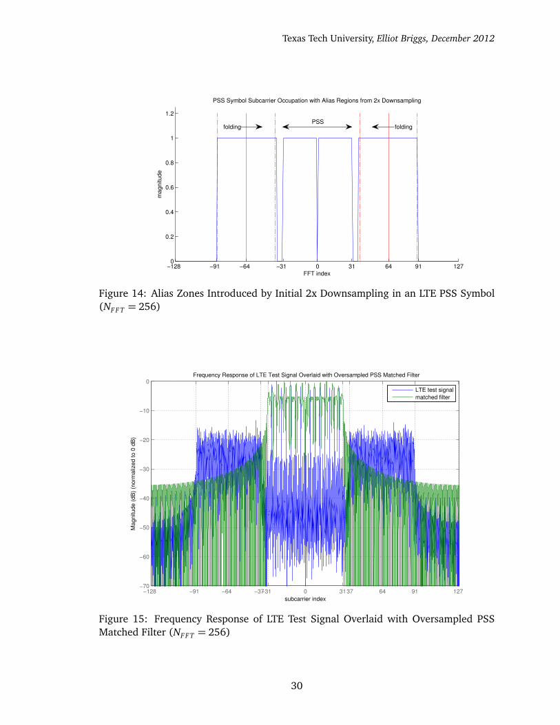
Texas Tech University, Elliot Briggs, December 2012
−128 −91 −64 −31 0 31 64 91 1270
0.2
0.4
0.6
0.8
1
1.2
FFT index
ma
gn
itu
de
PSS Symbol Subcarrier Occupation with Alias Regions from 2x Downsampling
folding foldingPSS
Figure 14: Alias Zones Introduced by Initial 2x Downsampling in an LTE PSS Symbol(NF F T = 256)
−128 −91 −64 −37−31 0 3137 64 91 127−70
−60
−50
−40
−30
−20
−10
0
subcarrier index
Magnitude (
dB
) (n
orm
aliz
ed to 0
dB
)
Frequency Response of LTE Test Signal Overlaid with Oversampled PSS Matched Filter
LTE test signal
matched filter
Figure 15: Frequency Response of LTE Test Signal Overlaid with Oversampled PSSMatched Filter (NF F T = 256)
30

Texas Tech University, Elliot Briggs, December 2012
downsampled, thus the matched filter and the signal both retain their correlation prop-
erties. However, another downsampling operation by 2, reducing the matched filtering
operation to the minimum possible sampling rate, aliases the data subcarriers to the
PSS location, and therefore a traditional band limiting or polyphase downsampler must
be used to prevent such interference.
Whether by design or coincidence, the initial no-cost 2x downsampling operation
never aliases over the PSS locations in all FFT sizes and bandwidth configurations
available in the LTE downlink (NF F T = 2n, n ∈ {7,8, 9,10, 11}), always allowing a
no-cost downsampling stage to initially reduce the sampling rate by 2. To further
reduce the workload in each FFT configuration, successive FIR downsampling can be
performed to allow constant minimum-rate PSS correlation.
The goal of this multi-rate design is to perform matched filtering at a constant and
minimum possible rate across all LTE bandwidth modes and FFT sizes. Starting with the
smallest FFT size and its corresponding sampling rate, the minimum-rate matched filter
bank is generated by populating 128-element IFFT operations with the three possible
63-element frequency domain ZC sequences. The filter generated by a minimum-sized
64-element IFFT could be used for minimum-rate processing, however for NF F T > 128,
the required downsampling filter must have an excessively narrow transition band to
fit inside the gap provided by the 5 null subcarriers surrounding the PSS. The narrow
transition band requires a high filter order in order to not degrade the correlation, high
enough that oversampled PSS correlation is justified.
For NF F T = 128, no rate transition is used, and the matched filter is oversampled
by a factor of 2. For NF F T = 256, the matched filter bank is preceded by the no-cost 2x
downsampling operation. For each FFT size greater than 256, a 2x polyphase down-
sampler is added, creating a chain, or dyadic cascade of filters. Each filter only needs to
suppress frequencies that alias into the PSS location after its respective downsampling.
The overlaid frequency response of the entire filter chain is displayed in Fig. 16. Each
filter is designed to be a half-band filter, a special Nyquist filter that has zeros for nearly
half of its coefficient set, which provides a very efficient polyphase implementation and
reduces the coefficient storage requirement by a factor of 2.
The cascaded filter response in Fig. 17 appears to show a particularly underwhelm-
ing frequency response. Large lobes emerge from the stop-band and the transition
band is nowhere near “sharp”. However, the filter gives excellent performance where
needed, not allowing interference to alias over the PSS while reducing the sampling
rate to a constant rate for a fixed matched filter bank, and using the minimum number
of computations to do so.
31
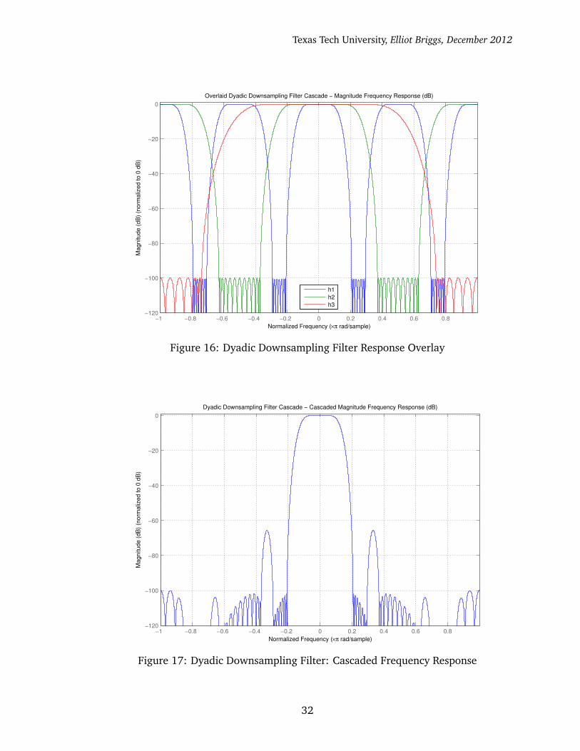
Texas Tech University, Elliot Briggs, December 2012
−1 −0.8 −0.6 −0.4 −0.2 0 0.2 0.4 0.6 0.8−120
−100
−80
−60
−40
−20
0
Normalized Frequency (×π rad/sample)
Ma
gn
itu
de
(d
B)
(no
rma
lize
d t
o 0
dB
)
Overlaid Dyadic Downsampling Filter Cascade − Magnitude Frequency Response (dB)
h1
h2
h3
Figure 16: Dyadic Downsampling Filter Response Overlay
−1 −0.8 −0.6 −0.4 −0.2 0 0.2 0.4 0.6 0.8−120
−100
−80
−60
−40
−20
0
Normalized Frequency (×π rad/sample)
Magnitude (
dB
) (n
orm
aliz
ed to 0
dB
)
Dyadic Downsampling Filter Cascade − Cascaded Magnitude Frequency Response (dB)
Figure 17: Dyadic Downsampling Filter: Cascaded Frequency Response
32

Texas Tech University, Elliot Briggs, December 2012
PSS0 MF
PSS2 MF
PSS1 MF
max
0
1
2
Sector ID
maxSymbol Timing Estimate
z-M1
H1,1
bypass2
0
1 z-M2
H2,1
bypass3
0
1 z-M3
bypass4
0
1
H3,1
2:1RX
bypass1
0
1
Figure 18: Dyadic Downsampling Filter with Matched Filter Bank: Implemented Struc-ture
Filter Input Sampling Rate Coefficient Storage Workload Cumulative Workload(MHz) (samples) (MMACCs/s) (MMACCs/s)
PSS0 1.92 65 245.76 (complex) 245.76PSS1 1.92 65 245.76 (complex) 491.52PSS2 1.92 65 245.76 (complex) 737.28h3 3.84 4 30.72 (real) 768h2 7.68 6 92.16 (real) 860.16h1 15.36 6 184.32 (real) 1,042.48h0 30.72 0 0 1,042.48
Table 2: Multi-Rate PSS Detector Computation and Coefficient Storage Requirements
Fig. 18 illustrates the implemented structure of the PSS detector at this point, show-
ing the cascade of 2x downsampling components, each separated by a bypass multi-
plexer used for selecting the appropriate rate transition for the incoming sampling rate
and respective FFT size. The multiplexers allow the final sampling rate to be constant,
regardless of the wide range of input sampling rates, allowing the matched filter bank
to operate with constant coefficients and at a constant rate.
A breakdown of the filter’s workload is listed in Tbl. 2. The cascaded design allows
each filter to work at a constant rate when enabled, simplifying the system’s workload
analysis. At the given workload, each of the matched filters can be implemented us-
ing a single complex MACC element in a Xilinx Virtex7 FPGA, each complex MACC
element requiring 6 DSP48E1 FPGA slices [26]. Two block RAMs (BRAMs) are re-
quired to store the coefficients of the symmetric matched filters, two of which are com-
33

Texas Tech University, Elliot Briggs, December 2012
−1 −0.8 −0.6 −0.4 −0.2 0 0.2 0.4 0.6 0.8−120
−100
−80
−60
−40
−20
0
Normalized Frequency (×π rad/sample)
Ma
gn
itu
de
(d
B)
(no
rma
lize
d t
o 0
dB
)
Overlaid Dyadic Upsampling Filter Cascade − Magnitude Frequency Response (dB)
h4
h5
h6
h7
Figure 19: Dyadic Upsampling Filter Response Overlay
plex conjugates of each other, eliminating the need for a third BRAM. The remaining
polyphase downsamplers require too few coefficients to justify using valuable BRAM
elements. Coefficient storage should be relegated to discrete registers. The low work-
load of each of the polyphase downsamplers in the cascade can be implemented using
a single DSP48E1, capable of realistically providing 250 MMACs/s. Summing up the
required resources, the downsamplers with matched filter bank should occupy approx-
imately 21 DSP48E1 elements and 3 BRAMs with some ancillary logic elements. The
DSP48E1 usage accounts for a mere 1.6% of the available elements in the smallest
Xilinx Virtex7 DSP-targeted FPGA.
The PSS detection performs admirably at this point in the design, capable of de-
tecting the correct sector ID in any of the possible sampling rates. A direct comparison
with the overlap-add method cannot yet be made. The output rate of the overlap-add
method is equal to its input. A side effect of the downsampling process in the multi-rate
design is reduced symbol timing resolution. To restore the original time resolution in
all operating sampling rates, variable power-of-2 upsampling can be performed in the
same manner as the downsampling direction, using a dyadic upsampling filter cascade
of half-band polyphase upsampling filters.
Fig. 19 shows the overlaid frequency response of the designed filter cascade at
the respective relative sampling rates. The upsampling filter has a more difficult job
34

Texas Tech University, Elliot Briggs, December 2012
−1 −0.8 −0.6 −0.4 −0.2 0 0.2 0.4 0.6 0.8
−140
−120
−100
−80
−60
−40
−20
0
Normalized Frequency (×π rad/sample)
Magnitude (
dB
) (n
orm
aliz
ed to 0
dB
)
Dyadic Upsampling Filter Cascade − Full Cascaded Magnitude Frequency Response (dB)
Figure 20: Dyadic Upsampling Filter: Cascaded Frequency Response
Filter Input Sampling Rate Coefficient Storage Workload Cumulative Workload(MHz) (samples) (MMACCs/s) (MMACCs/s)
h4 1.92 8 61.44 (real) 61.44h5 3.84 8 122.88 (real) 184.32h6 7.68 4 122.88 (real) 307.20h7 15.36 3 184.32 (real) 491.52
Table 3: Dyadic Cascaded Upsampler Computation and Coefficient Storage Require-ments
than the downsampling portion. The upsampler must successively eliminate aliases
altogether, rather than eliminate aliases that only interfere with the PSS subcarriers.
The resulting filter design requires higher workloads in each stage. Fig. 20 shows the
cascaded frequency response of the upsampler.
Fig. 21 shows the udpated design with the attached upsampler cascade. The trans-
posed multiplexer shows that either multiplexer configurations can be used in the de-
sign. The “max” component is now moved to the output of the upsampler chain to
take advantage of the unit-input sample time resolution achieved by the upsampling
operation.
The breakdown of the upsampler’s workload is shown in Tbl. 3. Like the downsam-
35

Texas Tech University, Elliot Briggs, December 2012
PSS0 MF
PSS2 MF
PSS1 MF
max
0
1
2
Sector ID
z-M1
H1,1
bypass2
0
1 z-M2
H2,1
bypass3
0
1 z-M3
bypass4
0
1
H3,1
2:1RX
bypass1
0
1
z-M4 z-M5 z-M6 z-M7
1 2 3 4Mode
max(position)
Symbol Timing Estimate
H4,1 H5,1 H6,1 H7,1
Figure 21: Multi-Rate PSS Detection Algorithm: Implemented Processing Structure
pler, the required coefficient storage space is very small, too small to waste valuable
BRAM in the FPGA, and general-purpose registers are a better choice. Also as with the
downsampler, each stage can be implemented using a single DSP48E1 MACC element,
totaling 4 in the entire design.
Analyzing Tbl. 2 and 3, and considering the anticipated hardware resource con-
sumption, it is hard to imagine that the overlap-add method can achieve better results.
The time-domain results in Fig. 22 show the overlaid outputs of the multi-rate overlap-
add techniques. The overlap-add output is generated using MATLAB’s “fftfilt” function.
Expectedly, the resulting output sequences of the two techniques are quite similar. In
this example, the signal is generated according to the LTE specification using N (2)I D = 0,
and NF F T = 2048. The two PSS symbols are spaced by 5 ms in a single 10 ms radio
frame, according to the 20 MHz LTE mode of operation in the FDD format. In this
example, the overlap-add method uses a pair of 32,768 point inverse and forward FFTs
and an overlap of 2,047 samples, the automatically chosen ideal size by MATLAB’s fft-
filt function. Using this configuration, the overlap-add algorithm progresses through
the time series in strides of 30,721 samples, completing approximately 1,000 strides
per second. According to the fftfilt function, each (I)FFT operation requires 1,441,974
36

Texas Tech University, Elliot Briggs, December 2012
1.528 1.53 1.532 1.534 1.536 1.538 1.54 1.542 1.544
x 104
0
0.2
0.4
0.6
0.8
1
sample index (time)
magnitude−
square
d
polyphase cascade
fftfilt
0 0.5 1 1.5 2 2.5 3
x 105
0
0.2
0.4
0.6
0.8
1
sample index (time)
magnitude−
square
d
Multi−Rate vs. Overlap−Add PSS Correlation
polyphase cascade
fftfilt
Figure 22: Multi-Rate vs. Overlap-Add PSS Correlation
floating-point operations (flops).
The breakdown analysis for the overlap-add PSS detection algorithm is listed in
Tbl. 4. The total sustained workload of 6.37 Gflops/s would require the theoretical per-
formance of almost 40 Cray I supercomputers from the year 1976, each capable of 160
Mflops/s [27]. Summing up the computations required for root index 25 matched fil-
tering, given in Tbl. 2 and 3, and assuming a complex MACC requires 8 Flops and a real
MACC requires 2, the total workload of the multi-rate design requires 5.26 Gflops/s,
or nearly 33 Cray I computers.
In addition to fewer computations, the multi-rate design has several other advan-
tages. The inner argmax term in Eq. 13 can be performed at the minimum rate. As a
result, the outer argmax term must only be evaluated on an individual output stream,
resulting in a two-thirds complexity reduction factor vs. the overlap-add method. The
multi-rate design also has a very low coefficient storage requirement, requiring only 39
real and 130 complex coefficients. Each of the filters used in the overlap-add technique
has 215 elements, which can be computed from smaller coefficient sets, however the
full-sized filter coefficients must reside in memory during operation. In addition to the
37
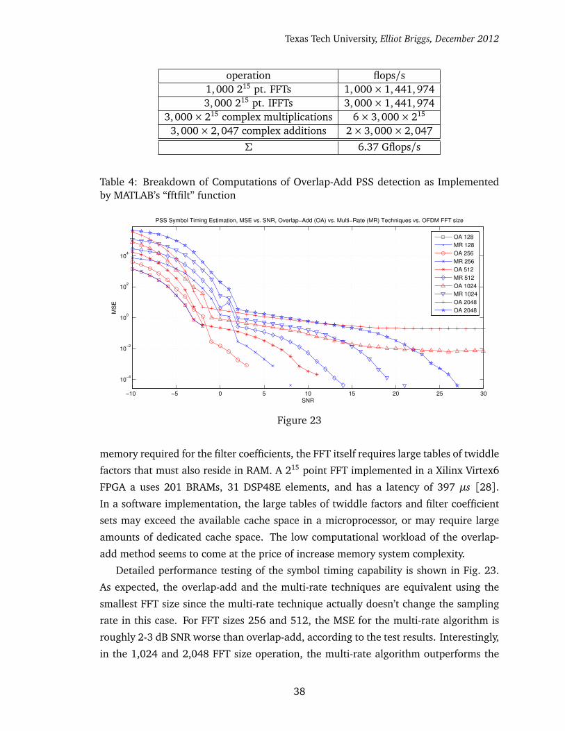
Texas Tech University, Elliot Briggs, December 2012
operation flops/s1,000 215 pt. FFTs 1, 000× 1,441, 9743,000 215 pt. IFFTs 3, 000× 1,441, 974
3, 000× 215 complex multiplications 6× 3, 000× 215
3, 000× 2,047 complex additions 2× 3,000× 2, 047
Σ 6.37 Gflops/s
Table 4: Breakdown of Computations of Overlap-Add PSS detection as Implementedby MATLAB’s “fftfilt” function
−10 −5 0 5 10 15 20 25 30
10−4
10−2
100
102
104
PSS Symbol Timing Estimation, MSE vs. SNR, Overlap−Add (OA) vs. Multi−Rate (MR) Techniques vs. OFDM FFT size
SNR
MS
E
OA 128
MR 128
OA 256
MR 256
OA 512
MR 512
OA 1024
MR 1024
OA 2048
OA 2048
Figure 23
memory required for the filter coefficients, the FFT itself requires large tables of twiddle
factors that must also reside in RAM. A 215 point FFT implemented in a Xilinx Virtex6
FPGA a uses 201 BRAMs, 31 DSP48E elements, and has a latency of 397 µs [28].
In a software implementation, the large tables of twiddle factors and filter coefficient
sets may exceed the available cache space in a microprocessor, or may require large
amounts of dedicated cache space. The low computational workload of the overlap-
add method seems to come at the price of increase memory system complexity.
Detailed performance testing of the symbol timing capability is shown in Fig. 23.
As expected, the overlap-add and the multi-rate techniques are equivalent using the
smallest FFT size since the multi-rate technique actually doesn’t change the sampling
rate in this case. For FFT sizes 256 and 512, the MSE for the multi-rate algorithm is
roughly 2-3 dB SNR worse than overlap-add, according to the test results. Interestingly,
in the 1,024 and 2,048 FFT size operation, the multi-rate algorithm outperforms the
38

Texas Tech University, Elliot Briggs, December 2012
overlap-add algorithm in higher SNRs, crossing over at approximately 13-14 dB SNR
in both configurations. In these configurations, the multi-rate algorithm significantly
outperforms the overlap-add in high SNR conditions, where the MSE produced by the
overlap-add algorithm flattens out to a near-constant level, becoming independent of
SNR. The test was performed using fully occupied PSS/data OFDM symbols according
the LTE specification, totaling 24,000 PSS symbol detections for each data point.
3.5 Concluding Remarks
Receiver synchronization using time domain measurements allows the receiver to be
compartmentalized, relying solely on pre-FFT information. In the case of sampling
clock frequency synchronization, time domain measurements offer many benefits that
not only simplify the receiver’s architecture but also eliminate any dependency on post-
FFT information, which itself is fundamentally dependent on synchronization perfor-
mance. In the analysis of symbol timing synchronization, it was shown that sampling
frequency errors and symbol timing errors are co-related, and a receiver architecture
was developed that simultaneously synchronizes both. The proposed receiver architec-
ture illustrated admirable performance on the most generic OFDM system, using only
CP-derived symbol timing information.
To enhance timing and sampling frequency error measurements in an LTE downlink
receiver, the PSS is detected in the time domain using an efficient multi-rate architec-
ture. The computational workload was shown to be less than that of a technique known
for efficiently implementing long-length filters, the overlap-add algorithm.
Despite the depth of content in this chapter, critical components that have been
left undiscussed, particularly involving carrier frequency offset (CFO) correction. CFO
and SCO both produce SNR-degrading ICI [29]. CFO correction is well-studied and
can even be performed using the previously mentioned Beek algorithm. Many papers
present time-domain CFO correction techniques that align with the established design
principles in the presented receiver architecture [10,13,30,31].
39
Texas Tech University, Elliot Briggs, December 2012
4 OFDM Channel Estimation and Equalization
OFDM is well known for its simple single-tap equalization procedure (Eq. 179). While
the equalization procedure is trivial, obtaining (estimating) the equalization matrix can
be the most computationally intensive portion of an OFDM receiver. The process of
estimating the equalization matrix must be preceded by estimating the channel’s fre-
quency response, i.e. Eq. 176, 177. The equalization matrix is obtained by inverting
the diagonal frequency response matrix, i.e. Eq. 178.
In an OFDM receiver, the exact values that make up H1 in Eq. 174, or more concisely,
the channel impulse response vector h that comprises H1, is unknown and must be
estimated using the received signal. Usually, reference symbols (RSs) are inserted into
the OFDM symbol vector that give the receiver a foothold for directly estimating the
equalization matrix E. If the transmitted vector x(k) is known, v(k), the noisy channel
corrupted vesion of the transmitted signal is available.
v(k) =WMZRH1ZT WHMx(k) +WMZRn(k)
n(k) =WMZRn(k)
v(k) = Dx(k) + n(k)
(35)
The ideal equalization matrix E is obtained if the noise is explicitly known
E= D−1 = diag�
x(k)v(k)− n(k)
�
, (36)
which is impractical. More realistically, the receiver can obtain the least-squares solu-
tion
hLS =x(k)v(k)
ELS = diag�
hLS
(37)
This type of channel estimation is commonly referred to as the “least-squares” (LS)
estimator because ELS is the least-squares solution to the system of linear equations.
The LS estimator gives poor performance but has a very low computational complexity
when compared to other channel estimation techniques.
To improve the precision of the channel estimate in noisy conditions, the chan-
nel’s second-order statistics can be used to obtain the linear minimum-mean-squared
error (LMMSE) filter. After applying the filter, the LMMSE channel estimate is ob-
40
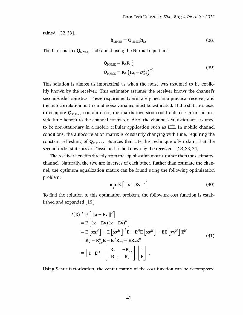
Texas Tech University, Elliot Briggs, December 2012
tained [32,33].
hMMSE = QMMSEhLS (38)
The filter matrix QMMSE is obtained using the Normal equations.
QMMSE = RhR−1hn
QMMSE = Rh
�
Rh+σ2nI�−1 (39)
This solution is almost as impractical as when the noise was assumed to be explic-
itly known by the receiver. This estimator assumes the receiver knows the channel’s
second-order statistics. These requirements are rarely met in a practical receiver, and
the autocorrelation matrix and noise variance must be estimated. If the statistics used
to compute QM MSE contain error, the matrix inversion could enhance error, or pro-
vide little benefit to the channel estimator. Also, the channel’s statistics are assumed
to be non-stationary in a mobile cellular application such as LTE. In mobile channel
conditions, the autocorrelation matrix is constantly changing with time, requiring the
constant refreshing of QM MSE. Sources that cite this technique often claim that the
second-order statistics are “assumed to be known by the receiver” [23,33,34].
The receiver benefits directly from the equalization matrix rather than the estimated
channel. Naturally, the two are inverses of each other. Rather than estimate the chan-
nel, the optimum equalization matrix can be found using the following optimization
problem:
minE
E�
‖ x− Ev ‖2�
(40)
To find the solution to this optimation problem, the following cost function is estab-
lished and expanded [15].
J(E)¬ E�
‖ x− Ev ‖2�
= E�
(x− Ev) (x− Ev)H�
= E�
xxH�
− E�
xvH�H
E− EHE�
xvH�
+ EE�
vvH�
EH
= Rx −RHx vE− EHRx v + ERvE
H
=h
1 EHi
Rx −Rvx
−Rx v Rv
1
E
.
(41)
Using Schur factorization, the center matrix of the cost function can be decomposed
41
Texas Tech University, Elliot Briggs, December 2012
into a product of upper-triangular, diagonal, and lower-triangular matrices.
Rx −Rvx
−Rx v Rv
=
1 −RvxR−1v
0 1
Rx −RvxR−1v Rx v 0
0 Rv
1 0
−R−1v Rx v 1
(42)
Substituting Eq. 42 into the result of Eq. 41 gives the expanded cost function.
J(E) =�
Rx −RvxR−1v Rx v
�
+�
E−R−1v Rx v
�HRv
�
E−R−1v Rx v
�
(43)
Since Rv is positive semi-definite, the equalization matrix that minimizes the cost func-
tion is
E= Eo = R−1v Rx v (44)
and the minimum mean-squared error is
Jmin = J(Eo) =m.m.s.e.=�
Rx −RvxR−1v Rx v
�
, (45)
One popular method to solve for the optimal equalization matrix Eo in Eq. 44 is to use
the steepest descent algorithm, which is widely known for its ability to start from an
initial guess for Eo and make interative improvements on the guess, ultimately converg-
ing on the true Eo. The general update procedure for the Steepest Descent algorithm is
given by
Ei = Ei−1+µPi, i ≥ 0 (46)
where each update is performed using the P matrix and the step size µ. Each P matrix
must be computed such that the cost decreases monotonically with each iteration, i.e.
J(Ei)< J(Ei−1) (47)
The update matrix P can be computed using the gradient of the cost function [15]
Pi =−�
∇J�
Ei−1
�H�H= Rx v −RvEi−1 , (48)
so that
Ei = Ei−1+µ�
Rx v −RvEi−1
�
, i ≥ 0 , E−1 = initial guess (49)
Also, the step size µ must satisfy the following condition to ensure Eq. 47
0< µ <2
λmax, (50)
42
Texas Tech University, Elliot Briggs, December 2012
where λmax denotes the largest eigenvalue of Rv.
A receiver rarely has knowlege of the correlation matrices Rx v and Rv, which are
usually time-varying. However, stochastic optimization techniques based on the steep-
est decent algorithm can be used to obtain the equalization matrix that approaches Eo
by estimating the second-order statistics. Both the algorithms in Eq. 44 and 39 perform
estimation assuming known statistics. If the statistics are estimated, the final product
is a result of two consecutive layers of estimates.
Stochastic optimization methods do not require the explicit knowledge of the second-
order statistics (correlation matrices) of the channel and yet can approach the optimum
solution over a sequence of iterations. The LMS algorithm operates similarly to the
steepest decent algorithm, except that the correlation matrices are approximated using
the instantaneous realization of the outer products. In the LMS algorithm, the expecta-
tion operator is removed, and the correlation matrices are approximated by performing
the respective outer products, i.e.
bRx v = xvH
bRv = vvH(51)
The LMS update equation can now be expressed as
Ei = Ei−1+µ�
xivHi − viv
Hi Ei−1
�
, i ≥ 0 , E−1 = initial guess , (52)
where the subscript i has been added to x and v to indicate the symbol index and the
step-size µ must satisfy Eq. 50.
Forcing E to be diagonal, the LMS algorithm in Eq. 52 approaches the optimal
value with finite steady-state error. Fig. 24 shows the results of the LMS algorithm
operating in the narrowest bandwidth LTE configuration, simultaneously estimating the
equalization coefficients for 24 RSs. The results show a wide variety of convergence
rates, ranging from near-instability to unreasonably slow. This effect is a result of
the differing relative step sizes, which depend on the input signal magnitudes. The
normalized LMS (NLMS) and ε-NLMS update the step sizes according to the magnitude
of the received signal, achieving equal convergence rates.
The LMS algorithm (and its variants) are derived using the steepest-descent tech-
nique, estimating the second-order statistics using instantaneous realizations. The re-
cursive least squares (RLS) algorithm alternatively arrives at the optimal solution using
Newton’s method, which recursively updates and improves its estimate of the second-
order statistics with each iteration. To provide tracking capability in time-variant con-
43
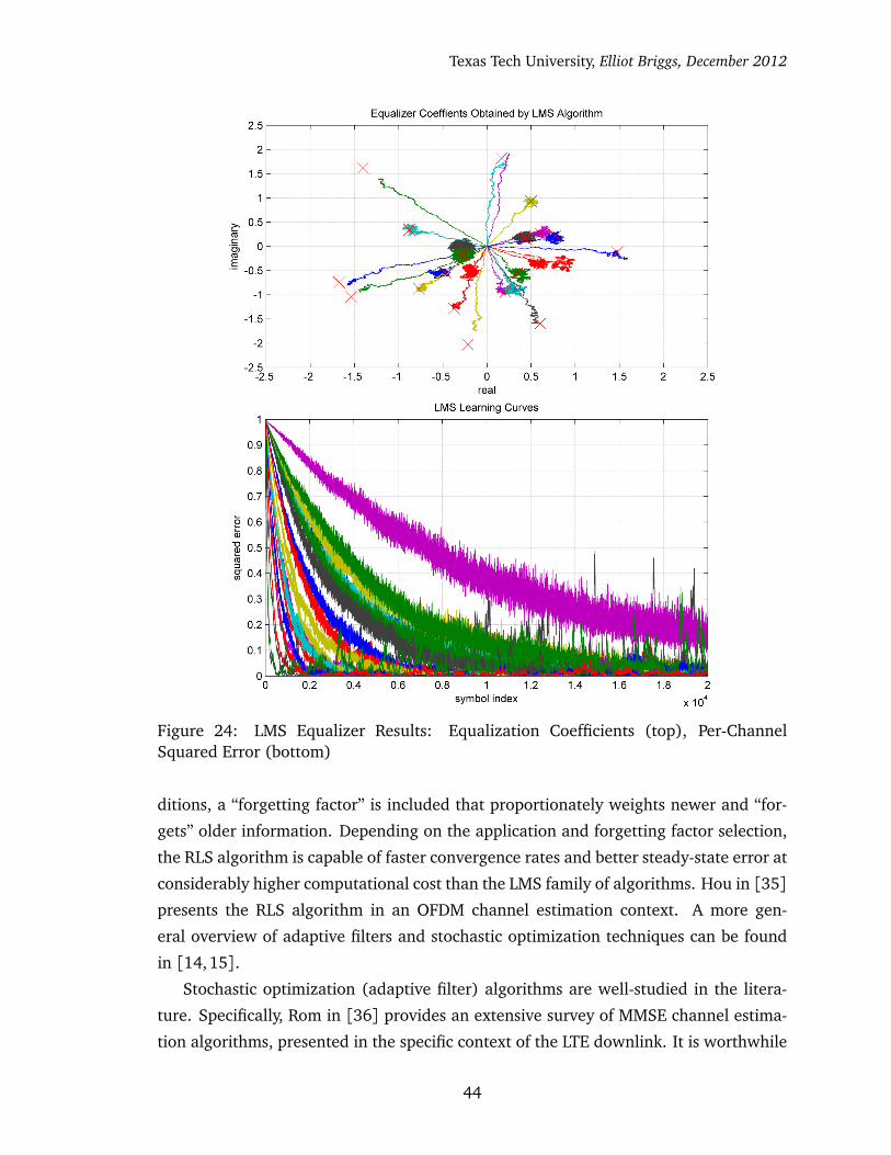
Texas Tech University, Elliot Briggs, December 2012
Figure 24: LMS Equalizer Results: Equalization Coefficients (top), Per-ChannelSquared Error (bottom)
ditions, a “forgetting factor” is included that proportionately weights newer and “for-
gets” older information. Depending on the application and forgetting factor selection,
the RLS algorithm is capable of faster convergence rates and better steady-state error at
considerably higher computational cost than the LMS family of algorithms. Hou in [35]
presents the RLS algorithm in an OFDM channel estimation context. A more gen-
eral overview of adaptive filters and stochastic optimization techniques can be found
in [14,15].
Stochastic optimization (adaptive filter) algorithms are well-studied in the litera-
ture. Specifically, Rom in [36] provides an extensive survey of MMSE channel estima-
tion algorithms, presented in the specific context of the LTE downlink. It is worthwhile
44

Texas Tech University, Elliot Briggs, December 2012
to consider an alternative class of algorithms that does not satisfy the MMSE optimality,
but are ML over the set of model parameters used to describe the signal. Unlike the
stochastic optimization algorithms that directly produce the equalization matrix, the
next approach estimates the channel.
4.1 Linear Regression Techniques for Channel Estimation
Assuming that an OFDM symbol contains training (reference) symbols (subcarriers), a
linear regression algorithm is a powerful tool that can be used to find the best-fit, or
ML parameter vector to fit the data using a given model [37–40].
Suppose it is desired to estimate or predict a value given the training vector y
observed at the coordinates indicated by the respective row in the matrix Z. Assuming
2 dimensions, the training set is indicated by the column vector z, which generates
the feature vector x using a mapping function. To model the data, the θ vector will
contain the coefficients of an mth order model. The coefficients that optimally fit the
data using the chosen model will be obtained through the learning algorithm. The
model is chosen to suit the anticipated properties of the data.
The function that maps the coordinates into the feature space defines the model.
As an example, let the θ vector contain coefficients of an mth order polynomial used to
describe y in the the feature space. The respective m× 1 vector x can be defined using
the elements of z.
x(i) =�
z0i ,z1
i , · · · ,zm−1i
�T(53)
Using the model parameter θ and the feature vectors, the prediction function generates
output values denoted by
by(i) = h�
x(i)�
= θ 0x(i)0 + θ 1x(i)1 + · · ·+ θm−1x(i)m−1 = θT x(i), 0≤ i ≤ n− 1 (54)
where n indicates the number of training variables and the vector and θ indicate the
obtained parameters used for prediction.
Using the entire set of feature vectors, the optimum parameter vector θ can be
found by constructing an n×m Vandermonde “design matrix”, X, using the x vectors
45

Texas Tech University, Elliot Briggs, December 2012
generated using the set of n training variables.
X=
—�
x(0)�T
—
—�
x(1)�T
—...
—�
x(n−1)�T
—
(55)
Using the established property that h�
x(i)�
= θ T x(i) =�
x(i)�Tθ , the error function for
a chosen θ vector can be established to be the difference between the prediction output
and the training.
Xθ − y=
�
x(0)�Tθ − y0
�
x(1)�Tθ − y1
...�
x(n−1)�Tθ − yn−1
=
h�
x(0)�
− y0
h�
x(1)�
− y1...
h�
x(n−1)�
− yn−1
(56)
To minimize the squared error, the following cost function parameterized by θ is es-
tablished.
J (θ ) =1
2
�
Xθ − y�2 (57)
To minimize J (θ ) with respect to θ , the gradient ∇θ J (θ ) can be found, set equal to
zero, and solved for θ to find the vector that optimizes the established cost fucntion,
θ opt .
∇θ J (θ ) =1
2∇θ�
�
Xθ − y�2�
=1
2∇θ�
�
Xθ − y�T �Xθ − y
�
�
=1
2∇θ�
θ T XT Xθ − θ T XT y− yT Xθ + yT y�
=1
2
�
2XT Xθ − 2XT y�
= XT Xθ −XT y
XT Xθ opt −XT y= 0
θ opt =�
XT X�−1
XT y .
(58)
To predict new target values, the optimum parameter vector θ opt is multiplied by the
46

Texas Tech University, Elliot Briggs, December 2012
design matrix X.
by= Xθ opt (59)
The X matrix in Eq. 59 contains the mapped coordinates of the predicted variable by.
While this linear regression technique is useful in general, it has several disadvan-
tages. When the contour of the data becomes increasingly detailed, the model order
must increase to produce low levels of prediction error. The number of computations
required to compute the m× m matrix inverse to obtain θ opt becomes prohibitive as
the model order increases. Another disadvantage to this algorithm is the equal weight-
ing of each element in the training set. Outliers and data with a great distance from
other data can introduce large bias errors throughout the entire regression space while
not having any significance to any data other than the data in the directly surrouding
region. In the machine learning context, performing regression using small windows of
data allows regression tasks to be performed using huge sets of training data without
having to process the set of data in its entirety.
To reduce the size of training data that must be processed to obtain a desired target
variable, windows of data directly surrounding the target variable location can be used
in place of the entire set. Using this concept with a local weighting kernel, a low-order
model can be used to compute locally optimum parameter vectors θ (i)opt for each target
variable. This operation can be implemented by adding a diagonal weight matrix to
the cost function that can be used to emphasize only the samples in close proximity to
the particular target variable.
J�
θ (i)�
=1
2
�
�
Xθ (i)− y�T
W�
Xθ (i)− y�
�
W= diag¦
w(i)©
(60)
The w vector contains the set of weights determined by the chosen weight kernel.
When W = I, the cost function collapses to Eq. 57. Alternatively, a popular kernel
exponentially decreases the influence of data points as they increase in distance from
the target variable location according to
w(i) = exp
−
�
x(i)− x�T �
x(i)− x�
2τ2
, (61)
which (coincidentally) cosmetically appears as the Gaussian kernel, where τ is the
47

Texas Tech University, Elliot Briggs, December 2012
“bandwidth” parameter that determines the width of the bell shaped function.
The new optimum θ (i)opt for this locally weighted regression (LWR) algorithm is found
using the cost function in Eq. 60,
∇θ J�
θ (i)�
=1
2∇θ�
�
Xθ (i)− y�T
W�
Xθ (i)− y�
�
=1
2∇θ�
�
θ (i)�T
XT WXθ (i)−�
θ (i)�T
XT Wy− yWXθ (i)+ yWy�
= XT WXθ (i)−XT Wy
XT WXθ (i)opt −XT Wy= 0
θ (i)opt =�
XT WX�−1
XT Wy
(62)
Each individual regression point at position i is computed using its correspoding θ (i)opt
by(i) = x(i)θ (i)opt (63)
At first, it may appear cumbersome to compute a θ (i)opt vector for each regression
output. With closer inspection, intriguing benefits of this algorithm are quickly re-
vealed. The most off-putting part of this algorithm is the requirement of an online
matrix inverse for each output; the weight kernel used to generate W must depend
on i. The XT WX term produces an m× m matrix, therefore when m = 2, the matrix
inversion is trivial using the following special property of 2× 2 matrices.
A−1 =1
det (A)
A(2,2) −A(1,2)
−A(2,1) A(1,1)
(64)
If online computation must take place, it must be noted that even m= 2 provides good
performance. When m= 2 and x(i) =�
z0i = 1,z1
i = zi
�T, θ (i)opt indicates the parameters
for the best-fit straight line for the weighted set of points. The first row of the resulting
X matrix is occupied by ones, and the second row is occupied by the z vector. The
row of ones causes the XT WX operation to require many multiplications by 1, an op-
eration that reduces to memory copies, significantly reducing the number of required
multiplications. Additionally, the XT W operation occurs twice in Eq. 62; the result can
be reused, further reducing the number of required computations. Perhaps the most
significant algorithmic simplification is obtained by exploiting the fact that the signifi-
48
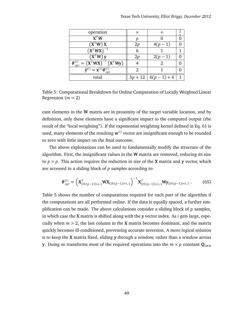
Texas Tech University, Elliot Briggs, December 2012
operation × + 1x
XT W p 0 0�
XT W�
X 2p 4(p− 1) 0�
XT WX�−1 6 1 1
�
XT W�
y 2p 2(p− 1) 0θ (i)opt =
�
XT WX�−1 �XT Wy
�
4 2 0by(i) = x(i)θ (i)opt 2 1 0
total 5p+ 12 6(p− 1) + 4 1
Table 5: Computational Breakdown for Online Computation of Locally Weighted LinearRegression (m= 2)
cant elements in the W matrix are in proximity of the target variable location, and by
definition, only these elements have a significant impact to the computed output (the
result of the “local weighting”). If the exponential weighting kernel defined in Eq. 61 is
used, many elements of the resulting w(i) vector are insignificant enough to be rounded
to zero with little impact on the final outcome.
The above exploitations can be used to fundamentally modify the structure of the
algorithm. First, the insignificant values in the W matrix are removed, reducing its size
to p× p. This action requires the reduction in size of the X matrix and y vector, which
are accessed in a sliding block of p samples according to:
θ (i)opt =�
XT((0:(p−1))+i,:)WX((0:(p−1))+i,:)
�−1XT((0:(p−1))+i,:)Wy((0:(p−1))+i,:) . (65)
Table 5 shows the number of computations required for each part of the algorithm if
the computations are all performed online. If the data is equally spaced, a further sim-
plification can be made. The above calculations consider a sliding block of p samples,
in which case the X matrix is shifted along with the y vector index. As i gets large, espe-
cially when m > 2, the last column in the X matrix becomes dominant, and the matrix
quickly becomes ill-conditioned, preventing accurate inversion. A more logical solution
is to keep the X matrix fixed, sliding y through a window, rather than a window across
y. Doing so transforms most of the required operations into the m× p constant QLWR
49

Texas Tech University, Elliot Briggs, December 2012
−15 −10 −5 0 5 10 150
0.1
0.2
0.3
0.4
0.5
0.6
0.7
0.8
0.9
1
Exponential Weighting Kernal with Varying τ Parameter (p=32)
offset
magnitude
τ=1
τ=2
τ=3
τ=4
τ=5
τ=6
Figure 25: Exponential Weighting Kernel with Varying τ Parameter
matrix.
θ (i)opt = QLWRy((0:(p−1))+i,:)
QLWR =�
XT WX�−1
XT W
X=
10 11 · · · 1m−1
20 21 · · · 2m−1
...... · · ·
...
p0 p1 · · · pm−1
by(i) = x(i)θ (i)opt
(66)
Now, the computation of the θ (i)opt vector requires only m�
p− 1�
additions, p (m− 1)
multiplications and no inverse operations. The modification enables higher orders of
m without the exponentially increasing cost of online matrix inversion and the issues
with ill-conditioned matrices.
To use this algorithm for channel estimation in an OFDM system, a kernel and its
corresponding value of p must be chosen. Fig. 25 displays the weighting function for
several values of the τ parameter in the exponential weighting kernel defined in Eq. 61.
While the kernel selection is somewhat arbitrary, the exponential kernel provides good
performance.
The chosen kernel and its parameters have a large impact on the performance of
50

Texas Tech University, Elliot Briggs, December 2012
50 100 150 200 250
−2
−1
0
1
2
τ=1
50 100 150 200 250
−2
−1
0
1
2
τ=2
50 100 150 200 250
−2
−1
0
1
2
τ=3
50 100 150 200 250
−2
−1
0
1
2
τ=4
50 100 150 200 250
−2
−1
0
1
2
τ=5
50 100 150 200 250
−2
−1
0
1
2
τ=6
LWR Results Using Varying τ Parameter, p=32
blue=signals+noise, green=signal, red=regression results
Figure 26: Overlaid Locally Weighted Regression Results with Varying τ Kernel Param-eter
the regression technique. The effects of the τ parameter on the regression results
using the exponential kernel is demonstrated in Fig. 26, showing 32 regression runs on
a signal with i.i.d. AWGN added to each experiment. The experiment is performed for
τ = [1, 2,3, 4,5, 6]. When τ = 1, the regression seems to “overfit” the signal, fitting
both the signal and its noise component. Conversely, when τ = 6, the regression is
unable to fit the “pointy” sections of the signal, producing regions of “underfitting”.
The τ that optimizes the MSE lies somewhere in-between 1 and 6. Once the optimum
value of τ is found, or learned either online, or using training data, the regression can
perform optimally on signals with similar characteristics.
If τ is swept in a similar manner as the previous experiment (displayed in Fig. 25)
51

Texas Tech University, Elliot Briggs, December 2012
1 2 3 4 5 60.022
0.024
0.026
0.028
0.03
0.032
0.034
0.036
0.038
0.04
τ
MS
E
MSE vs. Model Parameter τ
Figure 27: MSE vs. Model Parameter τ
and the computed MSE is used to measure the performance of the regression, the
relationship between τ and MSE as well as the optimum value of τ can be found.
Fig 27 shows the MSE for a sweep of the τ parameter from τ = [.7, .8, . . . , 6] using
the same signal with i.i.d. AWGN between each evaluation. The MSE is computed
using the known noiseless signal and the regression result. Clearly the MSE has a local
minimum around τ = 2 and perhaps most importantly, the sweep reveals a convex
error function.
To understand the relationship τ has with various types of signals, WGN is gener-
ated and upsampled by the variable rate N . Small N provides little upsampling, and
the resulting signals have sharper curvature and contour. WGN is also added to each
signal and is i.i.d. between each data point to corrupt the signals with noise. Fig. 28
shows the result of this experiment. The local minima are marked with a solid red cir-
cle for each sweep of τ with each N . Intuitively, the larger values of τ are better suited
for signals with more gradual contours, confirmed by Fig. 28 that showing that as N is
increased, the optimum value of τ that produces the minimum MSE also increased. For
signals with rapidly varying contours, choosing a large value for τ results in excessively
high absolute MSE, less so for signals with gradual contours. The relative MSE penalty
for excessively large values of τ is about equal within each trial between all N in this
experiment.
The previous experiment brings forth an interesting problem. Although data can
52
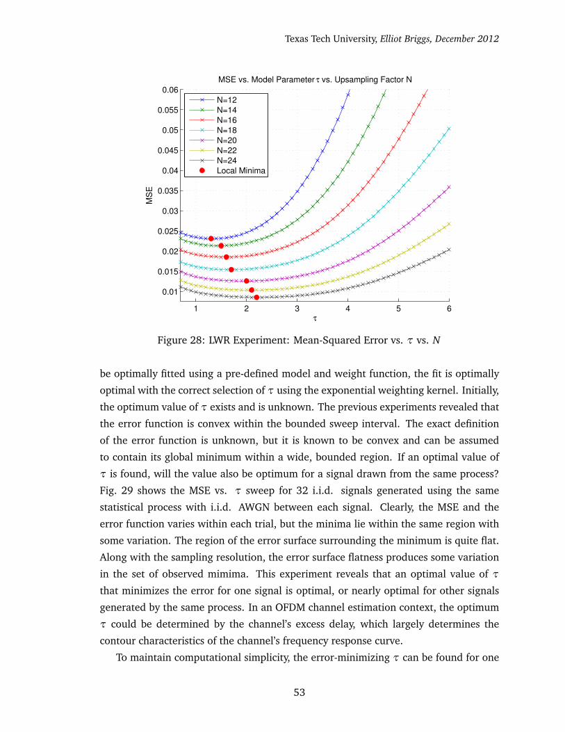
Texas Tech University, Elliot Briggs, December 2012
1 2 3 4 5 6
0.01
0.015
0.02
0.025
0.03
0.035
0.04
0.045
0.05
0.055
0.06
τ
MS
E
MSE vs. Model Parameter τ vs. Upsampling Factor N
N=12
N=14
N=16
N=18
N=20
N=22
N=24
Local Minima
Figure 28: LWR Experiment: Mean-Squared Error vs. τ vs. N
be optimally fitted using a pre-defined model and weight function, the fit is optimally
optimal with the correct selection of τ using the exponential weighting kernel. Initially,
the optimum value of τ exists and is unknown. The previous experiments revealed that
the error function is convex within the bounded sweep interval. The exact definition
of the error function is unknown, but it is known to be convex and can be assumed
to contain its global minimum within a wide, bounded region. If an optimal value of
τ is found, will the value also be optimum for a signal drawn from the same process?
Fig. 29 shows the MSE vs. τ sweep for 32 i.i.d. signals generated using the same
statistical process with i.i.d. AWGN between each signal. Clearly, the MSE and the
error function varies within each trial, but the minima lie within the same region with
some variation. The region of the error surface surrounding the minimum is quite flat.
Along with the sampling resolution, the error surface flatness produces some variation
in the set of observed mimima. This experiment reveals that an optimal value of τ
that minimizes the error for one signal is optimal, or nearly optimal for other signals
generated by the same process. In an OFDM channel estimation context, the optimum
τ could be determined by the channel’s excess delay, which largely determines the
contour characteristics of the channel’s frequency response curve.
To maintain computational simplicity, the error-minimizing τ can be found for one
53

Texas Tech University, Elliot Briggs, December 2012
1 2 3 4 5 60
0.01
0.02
0.03
0.04
0.05
0.06
0.07
0.08
0.09
0.1
τ
MS
E
MSE vs. Model Parameter τ − i.i.d. Trials with i.i.d. AWGN
Figure 29: MSE vs. Model Parameter τ: i.i.d. Trials with i.i.d. AWGN
signal and used for all other signals with similar characteristics. To find the optimum
τ, a search algorithm taken from convex optimization theory [41] can be employed to
evaluate the function for different values of the optimization parameter and selecting
the minimum (or maximum) result. A good search algorithm finds the minimum (or
maximum) value of a function using the fewest possible number of evaluations and
produces results with low error. Evaluating the error for a single sweep parameter
requires the regression operation to be performed on the entire data set, a computa-
tionally expensive operation, therefore it is critical to find the optimal parameter using
the fewest possible number of evaluations.
The error surface in the last few examples has shown a convex and apparently
a quadratic error function. To find the minimum of a quadratic function, inverse
quadratic interpolation can be performed, only requiring 3 function evaluations to ob-
tain the 3 necessary points for the interpolation and doesn’t require the explicit knowl-
edge of the function or its derivative. If the error function is assumed to be approx-
imately quadratic, the result of quadratic inverse interpolation will approximate the
location of the function’s minimum. The resulting accuracy depends on the validity of
the assumptions that are made. In many cases, the value produced by quadratic inverse
interpolation is “good enough” after only a few function evaluations. The objective of
54
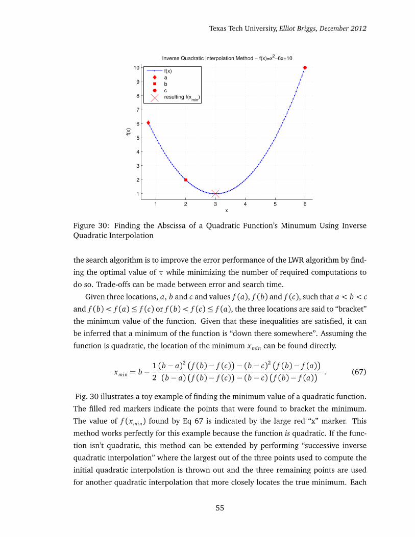
Texas Tech University, Elliot Briggs, December 2012
1 2 3 4 5 6
1
2
3
4
5
6
7
8
9
10
x
f(x)
Inverse Quadratic Interpolation Method − f(x)=x2−6x+10
f(x)
a
b
c
resulting f(xmin
)
Figure 30: Finding the Abscissa of a Quadratic Function’s Minumum Using InverseQuadratic Interpolation
the search algorithm is to improve the error performance of the LWR algorithm by find-
ing the optimal value of τ while minimizing the number of required computations to
do so. Trade-offs can be made between error and search time.
Given three locations, a, b and c and values f (a), f (b) and f (c), such that a < b < c
and f (b)< f (a)≤ f (c) or f (b)< f (c)≤ f (a), the three locations are said to “bracket”
the minimum value of the function. Given that these inequalities are satisfied, it can
be inferred that a minimum of the function is “down there somewhere”. Assuming the
function is quadratic, the location of the minimum xmin can be found directly.
xmin = b−1
2
(b− a)2�
f (b)− f (c)�
− (b− c)2�
f (b)− f (a)�
(b− a)�
f (b)− f (c)�
− (b− c)�
f (b)− f (a)� . (67)
Fig. 30 illustrates a toy example of finding the minimum value of a quadratic function.
The filled red markers indicate the points that were found to bracket the minimum.
The value of f (xmin) found by Eq 67 is indicated by the large red “x” marker. This
method works perfectly for this example because the function is quadratic. If the func-
tion isn’t quadratic, this method can be extended by performing “successive inverse
quadratic interpolation” where the largest out of the three points used to compute the
initial quadratic interpolation is thrown out and the three remaining points are used
for another quadratic interpolation that more closely locates the true minimum. Each
55

Texas Tech University, Elliot Briggs, December 2012
0 0.5 1 1.5 20.05
0.1
0.15
0.2
0.25
0.3
0.35
0.4
0.45
0.5
x
f(x)
Successive Inverse Quadratic Interpolation Method − f(x)=1/2−xe(−x
2)
f(x)
a
b
c
resulting f(xmin
(i))
Figure 31: Finding the Abscissa of an Arbitrary Function’s Local Minumum Using theSuccessive Inverse Quadratic Minimum Finding Technique
iteration costs only one additional function evaluation and converges to the true min-
imum super-linearly (quadratically). The algorithm can stop after the difference of
each result is smaller than a threshold value, or the maximum number of permissible
iterations has been exceeded. Fig. 31 shows the successive quadratic interpolation al-
gorithm finding the minimum of a non-quadratic function using 9 function evaluations
to achieve an accuracy within .01 of the true minimum location. Unfortunately, the
points used to bracket the minimum greatly impact this algorithm’s speed of conver-
gence, as one would expect.
An example training procedure that finds the optimum τ parameter uses a known
time-varying channel observed by an OFDM receiver, the LWR algorithm, and er-
ror feedback provided to the successive inverse quadratic minimum finding algorithm
(SIQMF). The test is performed using a 20 MHz LTE downlink OFDM signal that has
passed through an emulated multi-path fading channel using the LTE-specified ETU
model with a maximum Doppler frequency of 100 Hz. The ETU channel model pos-
sesses the greatest excess delay of the specified LTE channel models, therefore is very
frequency selective, preferring lower values of τ. The variance of the noise added to
the signal in this experiment is σ2 = .1.
Fig. 32 shows the results of the training experiment. The red curve in Fig. 32
shows the obtained minimum value of τ with an error tolerance of less than .01 and
56
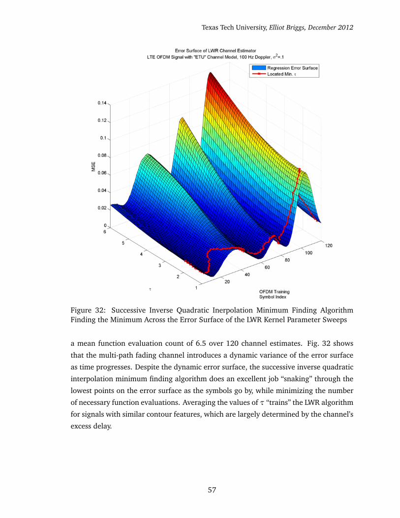
Texas Tech University, Elliot Briggs, December 2012
Figure 32: Successive Inverse Quadratic Inerpolation Minimum Finding AlgorithmFinding the Minimum Across the Error Surface of the LWR Kernel Parameter Sweeps
a mean function evaluation count of 6.5 over 120 channel estimates. Fig. 32 shows
that the multi-path fading channel introduces a dynamic variance of the error surface
as time progresses. Despite the dynamic error surface, the successive inverse quadratic
interpolation minimum finding algorithm does an excellent job “snaking” through the
lowest points on the error surface as the symbols go by, while minimizing the number
of necessary function evaluations. Averaging the values of τ “trains” the LWR algorithm
for signals with similar contour features, which are largely determined by the channel’s
excess delay.
57
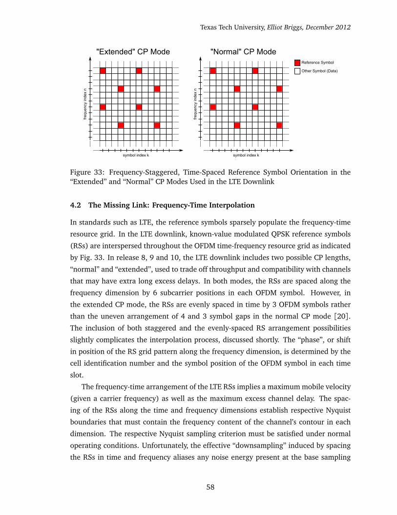
Texas Tech University, Elliot Briggs, December 2012
Reference Symbol
Other Symbol (Data)
freq
uenc
y in
dex
n
symbol index k
"Extended" CP Mode
freq
uenc
y in
dex
n
symbol index k
"Normal" CP Mode
Figure 33: Frequency-Staggered, Time-Spaced Reference Symbol Orientation in the“Extended” and “Normal” CP Modes Used in the LTE Downlink
4.2 The Missing Link: Frequency-Time Interpolation
In standards such as LTE, the reference symbols sparsely populate the frequency-time
resource grid. In the LTE downlink, known-value modulated QPSK reference symbols
(RSs) are interspersed throughout the OFDM time-frequency resource grid as indicated
by Fig. 33. In release 8, 9 and 10, the LTE downlink includes two possible CP lengths,
“normal” and “extended”, used to trade off throughput and compatibility with channels
that may have extra long excess delays. In both modes, the RSs are spaced along the
frequency dimension by 6 subcarrier positions in each OFDM symbol. However, in
the extended CP mode, the RSs are evenly spaced in time by 3 OFDM symbols rather
than the uneven arrangement of 4 and 3 symbol gaps in the normal CP mode [20].
The inclusion of both staggered and the evenly-spaced RS arrangement possibilities
slightly complicates the interpolation process, discussed shortly. The “phase”, or shift
in position of the RS grid pattern along the frequency dimension, is determined by the
cell identification number and the symbol position of the OFDM symbol in each time
slot.
The frequency-time arrangement of the LTE RSs implies a maximum mobile velocity
(given a carrier frequency) as well as the maximum excess channel delay. The spac-
ing of the RSs along the time and frequency dimensions establish respective Nyquist
boundaries that must contain the frequency content of the channel’s contour in each
dimension. The respective Nyquist sampling criterion must be satisfied under normal
operating conditions. Unfortunately, the effective “downsampling” induced by spacing
the RSs in time and frequency aliases any noise energy present at the base sampling
58
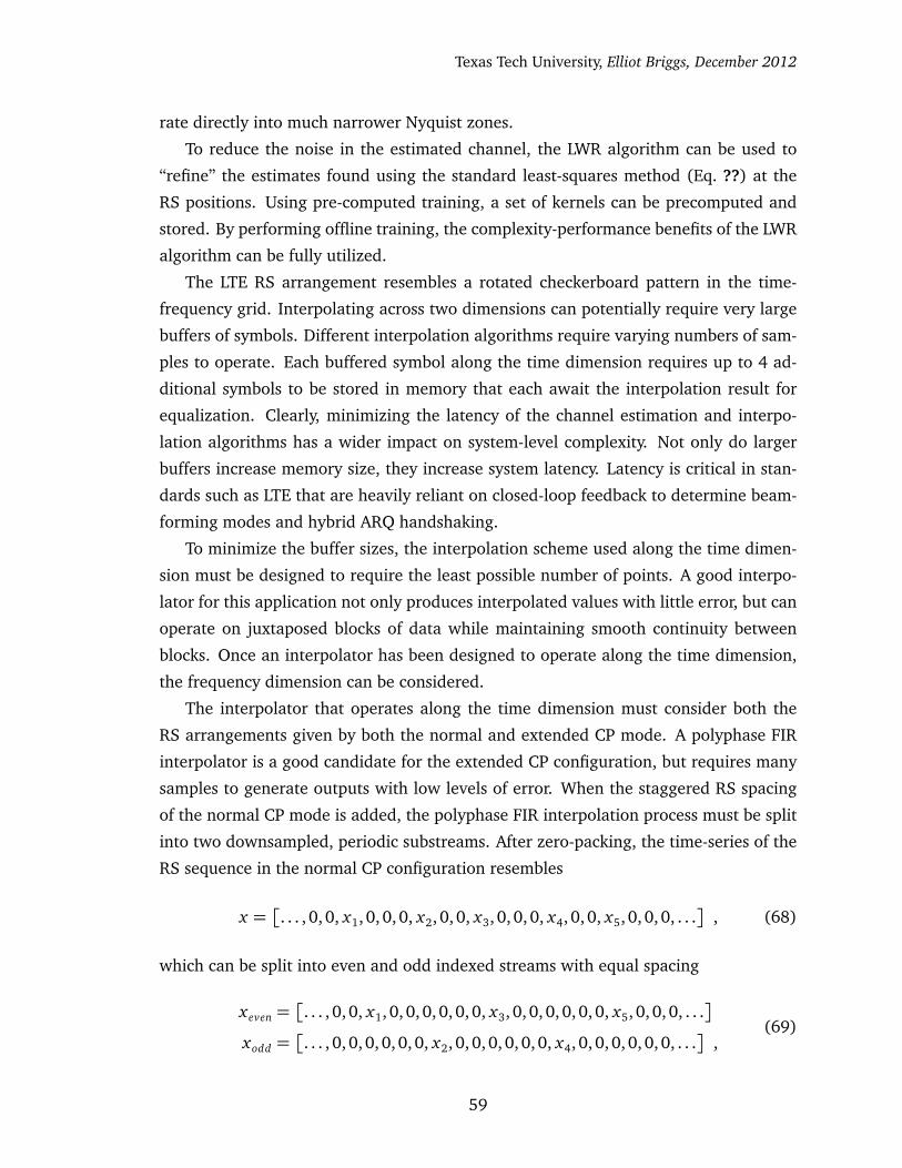
Texas Tech University, Elliot Briggs, December 2012
rate directly into much narrower Nyquist zones.
To reduce the noise in the estimated channel, the LWR algorithm can be used to
“refine” the estimates found using the standard least-squares method (Eq. ??) at the
RS positions. Using pre-computed training, a set of kernels can be precomputed and
stored. By performing offline training, the complexity-performance benefits of the LWR
algorithm can be fully utilized.
The LTE RS arrangement resembles a rotated checkerboard pattern in the time-
frequency grid. Interpolating across two dimensions can potentially require very large
buffers of symbols. Different interpolation algorithms require varying numbers of sam-
ples to operate. Each buffered symbol along the time dimension requires up to 4 ad-
ditional symbols to be stored in memory that each await the interpolation result for
equalization. Clearly, minimizing the latency of the channel estimation and interpo-
lation algorithms has a wider impact on system-level complexity. Not only do larger
buffers increase memory size, they increase system latency. Latency is critical in stan-
dards such as LTE that are heavily reliant on closed-loop feedback to determine beam-
forming modes and hybrid ARQ handshaking.
To minimize the buffer sizes, the interpolation scheme used along the time dimen-
sion must be designed to require the least possible number of points. A good interpo-
lator for this application not only produces interpolated values with little error, but can
operate on juxtaposed blocks of data while maintaining smooth continuity between
blocks. Once an interpolator has been designed to operate along the time dimension,
the frequency dimension can be considered.
The interpolator that operates along the time dimension must consider both the
RS arrangements given by both the normal and extended CP mode. A polyphase FIR
interpolator is a good candidate for the extended CP configuration, but requires many
samples to generate outputs with low levels of error. When the staggered RS spacing
of the normal CP mode is added, the polyphase FIR interpolation process must be split
into two downsampled, periodic substreams. After zero-packing, the time-series of the
RS sequence in the normal CP configuration resembles
x =�
. . . , 0, 0, x1, 0, 0, 0, x2, 0, 0, x3, 0, 0, 0, x4, 0, 0, x5, 0, 0, 0, . . .�
, (68)
which can be split into even and odd indexed streams with equal spacing
xeven =�
. . . , 0, 0, x1, 0, 0, 0, 0, 0, 0, x3, 0, 0, 0, 0, 0, 0, x5, 0, 0, 0, . . .�
xodd =�
. . . , 0, 0, 0, 0, 0, 0, x2, 0, 0, 0, 0, 0, 0, x4, 0, 0, 0, 0, 0, 0, . . .�
,(69)
59
Texas Tech University, Elliot Briggs, December 2012
which can be individually upsampled by a factor of 7 and summed to form the final
result. Theoretically, either the odd or even stream of samples by themselves could
be upsampled by 7 to obtain the needed result, but discarding information is never
advisable; therefore the two streams of samples will be upsampled and summed to
generate the final result.
Unfortunately, splitting the data into two separate sub-streams violates the Nyquist
conditions in the LTE-specified high speed train scenario, requiring a maximum Doppler
spread of 1340 Hz [42]. Assuming a classical Doppler spectrum, a channel null, or
deep fade for a particular subcarrier occurs at the time interval T0, determined by the
time the receiver takes to travel half the distance of the carrier’s wavelength (λ/2),
corresponding to double the Doppler frequency fd [43,44].
T0 =λ/2
v=
1/2
fd(70)
The time interval between RSs after splitting the single, unevenly spaced stream of RSs
into two substreams is equal to the duration of an entire LTE time slot, .5 ms, and can-
not resolve time variations caused by Doppler frequencies greater than fd = 1000 Hz.
To drive the point home even further, the polyphase FIR interpolator that performs
rate-7 upsampling requires a prohibitively large number of samples to compute each
output. Using the Remez filter design algorithm in MATLAB, a polyphase prototype
filter with an excess bandwidth parameter α = .3 and a stop-band attenuation of only
-60 dB requires 11 samples per polyphase arm; 11 RS-filled symbols must be stored
along with every other adjacent symbol that awaits equalization. Even in the extended
CP mode, where the data doesn’t need to be split and the Nyquist sampling criteria
is met by design, a rate-3 prototype filter requires 5 samples per polyphase arm for a
roughly -60 dB stop-band, given the same α. The stop-band attenuation and the α pa-
rameter could be relaxed even further for lower performance, but the required number
of samples that must be held in storage doesn’t compare to other more efficient and
higher performing algorithms, such as cubic spline interpolation.
Cubic spline interpolation is frequently used in 2-D interpolation tasks in image
processing, particularly for image scaling and rotation. Its main advantage is its ability
to fit data using low-order piece-wise polynomials with a continuous first and sec-
ond derivative between each piece. Spline interpolation has no restrictions on sample
spacing, making it an ideal class of interpolation algorithms for operating on both the
normal and extended RS grid configurations. The method used to compute the coeffi-
cients for each piecewise polynomial is quite simple, allowing a very computationally
60

Texas Tech University, Elliot Briggs, December 2012
efficient implementation. The mathematical background and theory of splines is well
established and will not be covered in detail here. The reader is referred to MATLAB’s
“spline”, “interp” and “interp2” functions for an implementation example, and [45] for
a thorough mathematical background.
The two cubic spline interpolation implementations present in the MATLAB func-
tions are the “clamped” and “not-a-knot” varieties. The clamped variety allows the 2nd
derivative to be explicitly specified at either end-point of the interpolation, and the
not-a-knot combines a single cubic for the first and last two subintervals. Either variety
can be implemented using a similar system of equations. The cubic spline interpolation
methods assign a continuous, piecewise polynomial segment for each contiguous set of
3 samples, defined by
fi(x) = ai + bi�
x − xi�
+ ci�
x − xi�2+ di
�
x − xi�3 , (71)
where i = 0, 1, . . . , n are the indices for the vector of ordered abscissas
xi =�
x0, x1, . . . , xn�T such that x0 < x1 < . . . < xn and vector of corresponding points
yi =�
y0, y1, . . . , yn�T . Each polynomial is evaluated using the ith element of the poly-
nomial coefficient vectors a,b,c,d and is valid for x i ≤ x ≤ x i+1. The polynomial
coefficient vectors can be solved using the linear equation
Am= r , (72)
where the m vector will be used to generate the four vectors of polynomial coefficients.
To define the A matrix, it is convenient to first introduce the vector hi = xi+1 − xi. For
the clamped spline method, the A matrix is defined
A=
2h0 h0 0 · · · · · · 0
h0 2�
h0+ h1
�
h1 0 · · · 0
0 h1 2�
h1+ h2
�
h2. . .
......
.... . . . . . . . .
...
0 0 0 hn−1 2�
hn−2+ hn−1
�
hn−1
0 0 0 0 hn−1 2hn−1
, (73)
61

Texas Tech University, Elliot Briggs, December 2012
followed by the r vector
r= 6
y1−y0
h0−δbegin
y2−y1
h1− y1−y0
h0...
yn−yn−1
hn−1− yn−1−yn−2
hn−2
δend −yn−yn−1
hn−1
, (74)
where δbegin and δend are the parameters used to force the derivative at the beginning
and end of each spline to a specific value. For the not-a-knot variant, the A matrix and
r vector are slightly modified. Note that the derivatives are known using the obtained
sets of piece-wise polynomials.
A=
−1 2 −1 · · · · · · 0
h0 2�
h0+ h1
�
h1 0 · · · 0
0 h1 2�
h1+ h2
�
h2. . .
......
.... . . . . . . . .
...
0 0 0 hn−1 2�
hn−2+ hn−1
�
hn−1
0 0 0 −1 2 −1
, (75)
r= 6
0y2−y1
h1− y1−y0
h0...
yn−yn−1
hn−1− yn−1−yn−2
hn−2
0
. (76)
Solving for the m vector in Eq. 72 allows for the computation of the vector of polyno-
mial coefficients.
m= A−1r (77)
ai = yi
bi =yi+1− yi
hi−
hi
2mi −
hi
6
�
mi+1−mi�
ci =mi
2
di =mi+1−mi
6hi
(78)
using i = 0,1, . . . , n− 1. A quick inspection of the A matrices for each method reveals
the following structures for evenly spaced sampling intervals. Given the RS spacing
62

Texas Tech University, Elliot Briggs, December 2012
along the time dimension in the extended CP mode, xi = [1, 4,7, ..., 3n+ 1]T , therefore
hi = [3, 3,3, ..., 3]T , resulting in
A=
6 3 0 · · · · · · 0
3 12 3 0 · · · 0
0 3 12 3...
......
.... . . . . . . . .
...
0 0 0 3 12 3
0 0 0 0 3 6
(79)
for the clamped algorithm and
A=
−1 2 −1 · · · · · · 0
3 12 3 0 · · · 0
0 3 12 3...
......
.... . . . . . . . .
...
0 0 0 3 12 3
0 0 0 −1 2 −1
(80)
for the not-a-knot. Note that the A matrix for the clamped algorithm is tridiagonal,
while the matrix for the not-a-knot algorithm is nearly so. There are very efficient
algorithms that can solve linear equations with matrices that have band-diagonal or
tridiagonal properties in O (n) operations [41], but these are unnecessary in the case
when the A matrix is constant and its inverse can be pre-computed, stored and multi-
plied by the dynamically updated r vector to solve for m. In the LTE RS configuration,
the RS spacing is periodic, allowing the A and its inverse matrix to be constant. Note
that the A−1 matrix varies with its dimensions, algorithm variety, and h. Also, the divi-
sion operations required by the r vector and Eq. 78 can be reduced to multiplications
by a pre-computed inverse or constant.
The cubic spline interpolation methods require a minimum of 4 points to be eval-
uated, therefore the minimum number of RS-filled symbols that must be stored along
the time dimension to perform interpolation between the RSs for both the extended
and normal CP modes is substantially fewer than the polyphase FIR interpolation tech-
nique. Using spline interpolation, only two slots (each consisting of 6 OFDM symbols
in the extended CP mode and 7 in the normal mode) must be stored to meet the 4
RS minimum along the time dimension, requiring 13 total symbols in the extended CP
63

Texas Tech University, Elliot Briggs, December 2012
100 200 300 400 500 600 700 800 900 1000 1100 12000
0.5
1
1.5
2
2.5
subcarrier index (frequency)
channel m
agnitude
Interpolation Using a 6x Polyphase FIR Filter
known channel
6x Polyphase Interpolation Result
Figure 34: Valid Output Samples of a Rate-6 Polyphase Upsampler Overlaid on theKnown Channel Magnitude
mode and 15 symbols in the normal CP mode.
A solution for interpolation along the frequency dimension is to use a rate-6 FIR
polyphase interpolator, which can finally be allowed to use large buffers of RSs. To
produce valid results, an FIR filter must keep its memory buffers filled with valid sam-
ples. As the memory buffer of the filter fills and empties, the resulting output exhibits
“settling” as only a portion of the full set of coefficients are contributing to the con-
volution output. The samples produced during the settling period of the filter are not
reliable and exhibit large deviations from the curvature of the input signal. In “nor-
mal use”, when an FIR interpolator operates an a infinitely long time series, assuming
no beginning and no end, these characteristics need not be considered, otherwise the
transients produced as the filter is settling must be dealt with. In this application, it
is best to simply trim any output samples that are computed when the filter’s memory
buffer isn’t completely filled. Fig. 34 illustrates the problem that the FIR filter interpo-
lator presents. The interpolator can’t produce valid outputs near the edges, or outer
subcarrier positions, otherwise the results are quite good for the interior subcarrier
indices.
64

Texas Tech University, Elliot Briggs, December 2012
Another possible solution to the interpolation problem is one that exploits the fact
that the channel’s frequency response, by definition from the FFT operation, is periodic
across the entire M block of samples produced by the receiver’s FFT operation. The
EDFT (extended discrete Fourier transform) algorithm introduced by [46] and avail-
able in [47] is specially designed to recover sparsely sampled periodic signals. The
algorithm doesn’t even require evenly spaced sampling and can recover signals with
large gaps of missing samples, a particularly attractive set of features considering the
channel’s frequency response in a typical OFDM signal is sparsely sampled only in the
central portion of the received frequency domain representation (the outer subcarriers
contain all zeros, i.e. the signal is oversampled). The algorithm is iterative, usually
requiring only a few iterations. The first iteration starts off using a diagonal weight
matrix G(1) = IM to produce the Hermitian Toeplitz matrix
R=1
NWMG(i)WH
M , (81)
where the WM matrix is the M × M DFT matrix that corresponds with the receiver’s
FFT (in this case, the samples are uniformly spaced). Next, using the weight matrix G
and the inverse R matrix, the complex i th estimate of the input signal vector x’s IDFT,
F(i) is computed.
F(i) = xR−1WMG(i) (82)
Next, to update the weight vector, the already computed xR−1WM and R−1WM terms
are used to generate the diagonal amplitude spectrum matrix S(i).
S(i) =xR−1WM
diag¦
WHMR−1WM
© (83)
G(i+1) = diag¦
|S(i)|2©
(84)
In normal circumstances, where an adequate number of RSs exist, the algorithm has
adequately converged after the 4th or 5th iteration when the identity matrix is used
as the initial weight vector. If the final weight vector from a previous result is used,
iterations typically end earlier. Vilinis in [47] stops the iterations when R becomes
ill-conditioned, or when the difference between successively computed F falls below a
set threshold. It should be noted that the R matrix has Toeplitz structure and can be
inverted using the computationally efficient Levinson-Durbin recursion in O (n) opera-
tions [48,49].
Fig. 35 illustrates an example OFDM symbol configuration (slightly different than
65
Texas Tech University, Elliot Briggs, December 2012
200 400 600 800 1000 1200 1400 1600 1800 20000
1
2
3
4
5
6
7
8
9
subcarrier index (frequency)
channel m
agnitude
EDFT Used for Recovering a Sparsely Sampled FFT − OFDM Channel Estimation
RS Locations
known channel
edft algorithm result
Figure 35: Interpolation and Gap-Filling of a Periodic Signal using the Extended DFTAlgorithm
the LTE configuration), which is sparsely sampled in the central subcarrier positions.
The given RSs are spaced periodically by 4 subcarrier indices. To assure a unique
solution, only the RSs are placed in the x vector and the FFT size is reduced from
2048 to 512, reducing the sampling rate so the portion of the signal given by the RSs
becomes critically sampled. This action prevents the algorithm from converging to a
solution that contains aliases (multiple solutions exist), or frequency multiples, while
reducing the computational complexity for each iteration. Size reduction is possible
when the starting FFT size is integer divisible by the RS spacing. Inconveniently, the
FFT size in the LTE configuration is not integer divisible by the 6-times undersampling
achieved by the RS spacing, therefore a preemptive upsampling by 3 operation should
be performed to allow optimal use of the EDFT algorithm. Once the algorithm has
operated on the downsampled RSs, zeros are inserted into the F matrix, which is then
multiplied by a full-sized DFT matrix, upsampling the result back to the original rate.
66
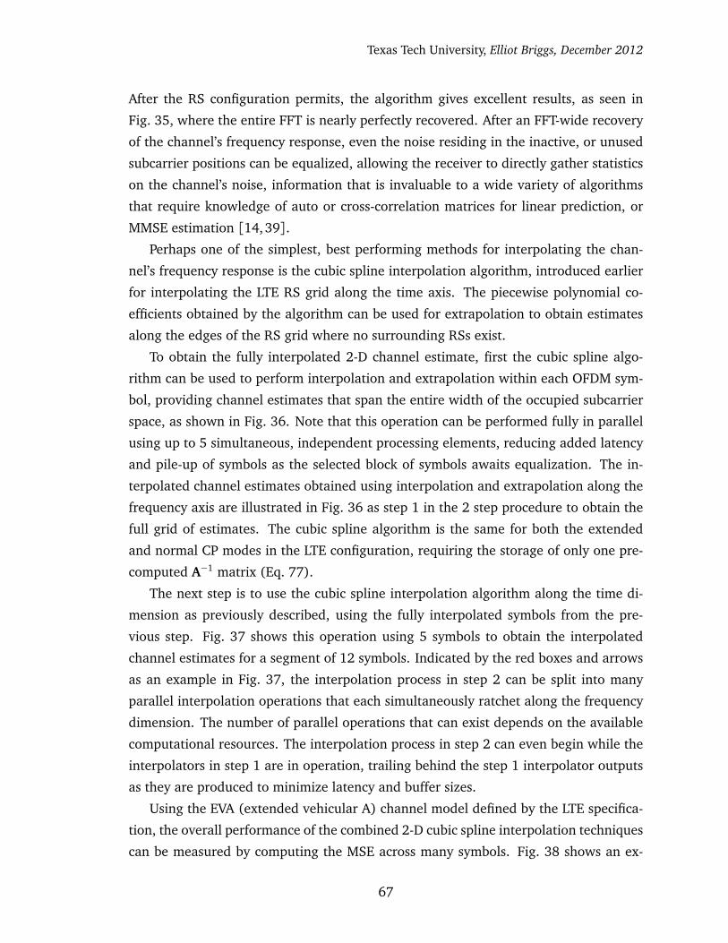
Texas Tech University, Elliot Briggs, December 2012
After the RS configuration permits, the algorithm gives excellent results, as seen in
Fig. 35, where the entire FFT is nearly perfectly recovered. After an FFT-wide recovery
of the channel’s frequency response, even the noise residing in the inactive, or unused
subcarrier positions can be equalized, allowing the receiver to directly gather statistics
on the channel’s noise, information that is invaluable to a wide variety of algorithms
that require knowledge of auto or cross-correlation matrices for linear prediction, or
MMSE estimation [14,39].
Perhaps one of the simplest, best performing methods for interpolating the chan-
nel’s frequency response is the cubic spline interpolation algorithm, introduced earlier
for interpolating the LTE RS grid along the time axis. The piecewise polynomial co-
efficients obtained by the algorithm can be used for extrapolation to obtain estimates
along the edges of the RS grid where no surrounding RSs exist.
To obtain the fully interpolated 2-D channel estimate, first the cubic spline algo-
rithm can be used to perform interpolation and extrapolation within each OFDM sym-
bol, providing channel estimates that span the entire width of the occupied subcarrier
space, as shown in Fig. 36. Note that this operation can be performed fully in parallel
using up to 5 simultaneous, independent processing elements, reducing added latency
and pile-up of symbols as the selected block of symbols awaits equalization. The in-
terpolated channel estimates obtained using interpolation and extrapolation along the
frequency axis are illustrated in Fig. 36 as step 1 in the 2 step procedure to obtain the
full grid of estimates. The cubic spline algorithm is the same for both the extended
and normal CP modes in the LTE configuration, requiring the storage of only one pre-
computed A−1 matrix (Eq. 77).
The next step is to use the cubic spline interpolation algorithm along the time di-
mension as previously described, using the fully interpolated symbols from the pre-
vious step. Fig. 37 shows this operation using 5 symbols to obtain the interpolated
channel estimates for a segment of 12 symbols. Indicated by the red boxes and arrows
as an example in Fig. 37, the interpolation process in step 2 can be split into many
parallel interpolation operations that each simultaneously ratchet along the frequency
dimension. The number of parallel operations that can exist depends on the available
computational resources. The interpolation process in step 2 can even begin while the
interpolators in step 1 are in operation, trailing behind the step 1 interpolator outputs
as they are produced to minimize latency and buffer sizes.
Using the EVA (extended vehicular A) channel model defined by the LTE specifica-
tion, the overall performance of the combined 2-D cubic spline interpolation techniques
can be measured by computing the MSE across many symbols. Fig. 38 shows an ex-
67

Texas Tech University, Elliot Briggs, December 2012
1 2 3 4 5 6 7 8 9 10 11 12 13 14 15 16 17 18 19 20 21 22 23 241
4
7
10
13
16
19
22
25
28
31
34
37
40
43
46
49
52
55
58
61
64
67
70
OFDM Symbol Index (time)
Su
bca
rrie
r In
de
x (
fre
qu
en
cy)
Step 1: Cubic Spline Interpolation/Extrapolation Along Frequency Dimension
Data Subcarrier Positions
RS
Obtained by Cubic Spline Interpolation
Obtained by Cubic Spline Extrapolation
Figure 36: Cubic Spline Interpolation/Extrapolation Along the Frequency Dimension(Step 1)
periment averaging the MSE over 4 frames (480 symbols). The lobes of increased MSE
appear when the curvature of the channel’s frequency response is more dynamic. Also
note that the MSE increases along the edges and in the middle subcarrier indices. The
indices along the edges are where extrapolation has been performed, as seen in Fig. 36.
The increase in MSE found in the centrally located indices is caused by the wider RS
spacing introduced by the DC subcarrier, which isn’t active in the LTE configuration. In
this area, the two RSs are spaced by 7 subcarrier positions rather than 6. Otherwise,
the performance of the cubic spline interpolation algorithm is excellent.
Next, the performance of the combined LWR and cubic splines interpolation algo-
rithms is evaluated. The test shown in Fig. 39 uses a kernel parameter obtained with
prior training on another simulation using the EVA (vehicular) channel model with
AWGN. In an implemented receiver, the proper kernel parameter must be chosen that
matches the available training scenarios. As previously suggested, the receiver can use
the measured excess delay of the channel to choose its kernel parameter. In this simu-
lation, the m parameter of the LWR algorithm is set to 3, allowing the algorithm to find
the best-fit parabola using the locally weighted data for each output. Increasing m al-
lows the kernel to be widened, including more data to generate each output. Because
68

Texas Tech University, Elliot Briggs, December 2012
1 2 3 4 5 6 7 8 9 10 11 12 13 14 15 16 17 18 19 20 21 22 23 241
4
7
10
13
16
19
22
25
28
31
34
37
40
43
46
49
52
55
58
61
64
67
70
OFDM Symbol Index (time)
Su
bca
rrie
r In
de
x (
fre
qu
en
cy)
Step 2: Cubic Spline Interpolation/Extrapolation Along Time Dimension
Data Subcarrier Positions
RS
Obtained by Cubic Spline Interpolation
Obtained by Cubic Spline Extrapolation
Figure 37: Cubic Spline Interpolation/Extrapolation Along the Time Dimension (Step2)
QLWR matrix is constant, the increase in m only linearly increases the computational
complexity. This particular test uses the Kaiser window as the kernel, which is pa-
rameterized by β . The Kaiser window’s parameter is normally used to trade transition
bandwidth for stopband attenuation in FIR filter design and spectral analysis; however
in this case the parameter is used to narrow and widen the window kernel. The Kaiser
window is defined by [24]:
w [n] =
I0
�
β(1−[(n−α)/α]2)1/2�
I0(β) 0≤ n≤ p
0 otherwise(85)
where β is the kernel parameter, α = p/2, and I0 (·) represents the zeroth-order mod-
ified Bessel function of the first kind. Fig. 39 illustrates the smoothing aspects of the
LWR technique and the good results given by the cubic splines interpolation method.
The LWR algorithm clearly smoothens the noisy LS channel estimates using the locally
best-fit parabolas generated using the Kaiser weighting kernel. The equalized result of
the test reveals the clear performance gains achieved by the LWR algorithm in Fig. 40,
69

Texas Tech University, Elliot Briggs, December 2012
0 200 400 600 800 1000 1200−90
−80
−70
−60
−50
−40
−30Cubic Spline Interpolation/Extrapolation MSE − EVA Channel Model
subcarrier index (frequency)
20
×lo
g10(M
SE
)
Figure 38: MSE of Cubic Spline Interpolation/Extrapolation Operating Under the EVAChannel Model
which shows the constellation of an LTE signal populated with QPSK modulated data
of 8 frames in duration, the EPA channel model with 100 Hz Doppler and added WGN
noise variance of σ2 = .001. The EPA channel model yields the best results due to its
low excess delay. Fig. 41 confirms that the excess delay is directly related to the perfor-
mance of the LWR estimator, which offers little to no improvement in the ETU model,
which has the largest excess delay. The test was performed using a full receiver, com-
plete with synchronization and the LTE RS arrangement. The results of both estimators
are interpolated to the full-sized frequency-time grid. This test was performed without
mobility. Fig. 41 shows the LWR estimator provided between 2-4 dB SNR improvement
from the LS method using the EPA and EVA models, each having 410 and 2510 ns
respective excess delays. Little improvement was attained by the LWR estimator when
using the ETU model with the longest excess delay of 5 µs.
70

Texas Tech University, Elliot Briggs, December 2012
600 800 1000 1200 1400 16000
0.2
0.4
0.6
0.8
1
1.2
1.4
1.6
DFT index (frequency)
magnitude
LWR Channel Estimator with Cubic Spline Interpolator − LTE RS Arrangement − EVA − σ2=.005
LS
LWR
Interpolated LS
Interpolated LWR
Figure 39: Comparison Between LWR and LS Algorithms Applied to LTE RS configura-tion with Cubic Splines Interpolator, EVA Channel Model, σ2 = .005
4.3 Reference Symbol Arrangements and Their Relationship with Timing Syn-
chronization
Reference symbols are usually interleaved in the same symbol with data subcarriers
and are not usually included in every transmitted symbol, requiring the receiver to
interpolate the channel’s response for the subcarrier positions that do not contain ref-
erence symbols. It is common that the receiver is required to interpolate along both
the time and frequency axes, as shown throughout this chapter.
In Fig. 33, the receiver is able to directly estimate the channel at the reference sym-
bol locations. Spacing the reference symbols apart in frequency and time brings forth
several new restrictions on timing synchronization. In Eq. 6, the relationship between
the continuous-time symbol timing offset parameter τ and the frequency-domain phase
shift vector φ is given. The channel estimation and equalization component allows
some timing synchronization error tolerance. The phase shifts induced by symbol tim-
ing errors can be absorbed into the channel’s frequency response. In the previous case
71
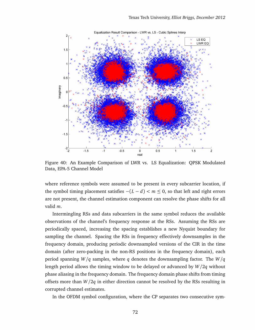
Texas Tech University, Elliot Briggs, December 2012
Figure 40: An Example Comparison of LWR vs. LS Equalization: QPSK ModulatedData, EPA-5 Channel Model
where reference symbols were assumed to be present in every subcarrier location, if
the symbol timing placement satisfies −(L − d) < m ≤ 0, so that left and right errors
are not present, the channel estimation component can resolve the phase shifts for all
valid m.
Intermingling RSs and data subcarriers in the same symbol reduces the available
observations of the channel’s frequency response at the RSs. Assuming the RSs are
periodically spaced, increasing the spacing establishes a new Nyquist boundary for
sampling the channel. Spacing the RSs in frequency effectively downsamples in the
frequency domain, producing periodic downsampled versions of the CIR in the time
domain (after zero-packing in the non-RS positions in the frequency domain), each
period spanning W/q samples, where q denotes the downsampling factor. The W/q
length period allows the timing window to be delayed or advanced by W/2q without
phase aliasing in the frequency domain. The frequency domain phase shifts from timing
offsets more than W/2q in either direction cannot be resolved by the RSs resulting in
corrupted channel estimates.
In the OFDM symbol configuration, where the CP separates two consecutive sym-
72

Texas Tech University, Elliot Briggs, December 2012
8 10 12 14 16 18 20 22 24 26 28
10−2
10−1
100
MSE Comparison of LS and LWR Channel Estimators Using LTE Channel Models
SNR
MS
E
EPA LS
EPA LWR
EVA LS
EVA LWR
ETU LS
ETU LWR
Figure 41: MSE Performance Comparison of LS and LWR Channel Estimators UsingLTE Channel Models
bols, symbol timing advancement induces ISI. Only symbol timing delay is possible
in ISI-free operation. The resolution boundary introduced by the RS spacing is com-
bined with the restrictions imposed by the channel’s excess delay to form the following
inequality
−�
min�
M
2q, (L− d)
��
< m≤ 0 , (86)
which must be satisfied by the symbol timing synchronization component to assure
correct operation.
In the LTE configuration, the RSs are separated by 5 subcarriers, downsampling
the channel’s frequency response by q = 6. Using M = 2048, the maximum valid
symbol timing offset is 170.67 samples. Additional timing offsets are possible if the
entire frequency domain symbol is purposefully phase-rotated by a known amount,
effectively shifting the valid symbol timing window in either direction.
The spacing of the reference symbols along time axis creates additional challenges
for symbol timing synchronization. The channel estimate may be updated for each
OFDM symbol that contains subcarriers with reference symbols. In many OFDM frequency-
73

Texas Tech University, Elliot Briggs, December 2012
time arrangements, the RSs are sparsely populated in both time and frequency. The
channel can only be estimated at the RS positions, which may not be present in every
OFDM symbol. In LTE, the RS-occupied symbols are spaced 3 and sometimes 4 sym-
bols apart (Fig. 33). The spacing in time requires the non-RS symbols to be equalized
by interpolated channel estimates using the adjacent RS-occupied symbols. The pre-
sented cubic spline interpolation technique requires a buffer of 4 RS symbols. If the
symbol timing is not constant within this buffer, the phase rotations will be disjointed
and the channel estimation result that spans between the RS symbols will be adversely
affected. The disjoint in symbol timing is especially detrimental to adaptive channel
estimators [33]. If the symbol timing must change, the phase of the frequency domain
vectors must be rotated accordingly to compensate for the known differential shifts in
timing.
4.4 Concluding Remarks
Designing a practical channel estimation algorithm requires the designer to make trade-
offs that greatly impact the performance and overall computational complexity apsects
of an OFDM receiver. An alternative to existing channel estimation techniques has been
presented that offers ML optimality rather than MMSE to trade performance for com-
plexity. Practical algorithms for frequency-time interpolation have also been presented
that consider the latency of the channel estimation and equalization components in the
receiver. Many aspects of the channel estimation and interpolation algorithms have
been distilled to use constant matrices, minimizing costly online matrix manipulations.
Finally, an important link between the timing synchronization and channel estimation
component was introduced that defines limitations that arise with sparse RS spacing
along the frequency axis.
74

Texas Tech University, Elliot Briggs, December 2012
5 Resampling Techniques Using Locally Weighted Linear Regression
Many additional and interesting uses for the LWR algorithm exist outside of the channel
estimation context.
In previous discussions, the LWR algorithm is used to “refine” noisy channel esti-
mates by smoothing them, followed by interpolation using the cubic splines algorithm
to obtain the full channel estimate in the frequency dimension. The LWR algorithm
finds coefficients for the best fit polynomial for each weighted set of samples. These
coefficients can be used to interpolate data between samples, replacing the function of
the cubic splines algorithm. The cubic splines algorithm guarantees a continuous 2nd
derivative connecting each polynomial, a feature the LWR algorithm does not provide.
However, using the LWR algorithm to perform interpolation as well as data smoothing
provides excellent results and a substantial reduction in computational workload if a
subsequent interpolation stage can be eliminated. To utilize the LWR algorithm’s inter-
polation capability, the optimal coefficient vector is computed as in Eq. 66, and the x(i)
vector is substituted with coordinates other than those given in the original set (hence
interpolation). Using the technique, the LWR algorithm is similar to cubic splines inter-
polation, such that the polynomial coefficient vectors are valid within a specific range
of coordinates. An example signal shown in Fig. 42 shows that the interpolation perfor-
mance is excellent. This example shows the LWR algorithm implemented with m = 4,
p = 32, and uses the Kaiser window as the kernel function. The example displays up-
sampling by a factor of 4. Notice the smoothness of the interpolated curve achieved
by fitting cubic polynomials, matching if not exceeding the performance of the cubic
spline interpolation algorithm. The LWR algorithm can be used to interpolate any co-
ordinate within the valid range of the computed best fit polynomials, enabling tasks
such as arbitrary-ratio resampling.
The LWR algorithm can be implemented using the constant QLWR matrix, eliminat-
ing an online matrix inversion and several matrix multiplications. If the possible struc-
ture of the implementated algorithm is considered, a striking resemblence is revealed.
75
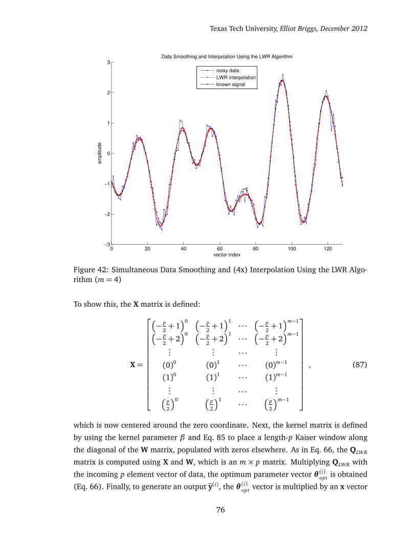
Texas Tech University, Elliot Briggs, December 2012
0 20 40 60 80 100 120−3
−2
−1
0
1
2
3
vector index
am
plit
ud
e
Data Smoothing and Interpolation Using the LWR Algorithm
noisy data
LWR interpolation
known signal
Figure 42: Simultaneous Data Smoothing and (4x) Interpolation Using the LWR Algo-rithm (m= 4)
To show this, the X matrix is defined:
X=
�
− p2+ 1�0 �
− p2+ 1�1· · ·
�
− p2+ 1�m−1
�
− p2+ 2�0 �
− p2+ 2�1· · ·
�
− p2+ 2�m−1
...... · · ·
...
(0)0 (0)1 · · · (0)m−1
(1)0 (1)1 · · · (1)m−1
...... · · ·
...�
p2
�0 �
p2
�1· · ·
�
p2
�m−1
, (87)
which is now centered around the zero coordinate. Next, the kernel matrix is defined
by using the kernel parameter β and Eq. 85 to place a length-p Kaiser window along
the diagonal of the W matrix, populated with zeros elsewhere. As in Eq. 66, the QLWR
matrix is computed using X and W, which is an m× p matrix. Multiplying QLWR with
the incoming p element vector of data, the optimum parameter vector θ (i)opt is obtained
(Eq. 66). Finally, to generate an output by(i), the θ (i)opt vector is multiplied by an x vector
76
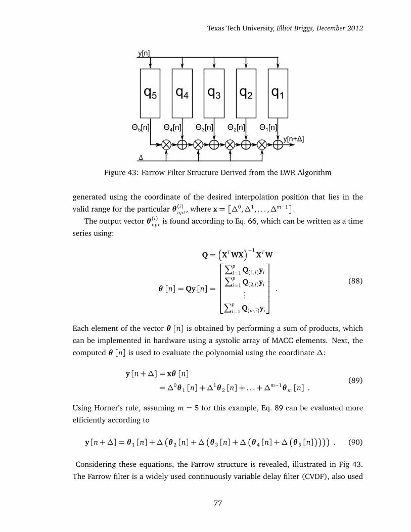
Texas Tech University, Elliot Briggs, December 2012
y[n+Δ]
Ɵ4[n] Ɵ3[n] Ɵ2[n] Ɵ1[n]
q5
Ɵ5[n]
Δ
y[n]
q4 q3 q2 q1
Figure 43: Farrow Filter Structure Derived from the LWR Algorithm
generated using the coordinate of the desired interpolation position that lies in the
valid range for the particular θ (i)opt , where x=�
∆0,∆1, . . . ,∆m−1�.
The output vector θ (i)opt is found according to Eq. 66, which can be written as a time
series using:
Q=�
XT WX�−1
XT W
θ [n] = Qy [n] =
∑pi=1 Q(1,i)yi
∑pi=1 Q(2,i)yi
...∑p
i=1 Q(m,i)yi
.(88)
Each element of the vector θ [n] is obtained by performing a sum of products, which
can be implemented in hardware using a systolic array of MACC elements. Next, the
computed θ [n] is used to evaluate the polynomial using the coordinate ∆:
y [n+∆] = xθ [n]
= ∆0θ 1 [n] +∆1θ 2 [n] + . . .+∆m−1θm [n] .
(89)
Using Horner’s rule, assuming m = 5 for this example, Eq. 89 can be evaluated more
efficiently according to
y [n+∆] = θ 1 [n] +∆�
θ 2 [n] +∆�
θ 3 [n] +∆�
θ 4 [n] +∆�
θ 5 [n]����
. (90)
Considering these equations, the Farrow structure is revealed, illustrated in Fig 43.
The Farrow filter is a widely used continuously variable delay filter (CVDF), also used
77

Texas Tech University, Elliot Briggs, December 2012
0 5−0.5
0
0.5
1
Q(1,:)
0 5−1
0
1
Q(2,:)
0 5−0.5
0
0.5
1
Q(3,:)
0 5−0.5
0
0.5
Q(4,:)
0 5−0.1
0
0.1
Q(5,:)
−0.5 0 0.50
0.5
1
1.5
f_Q(1,:)
−0.5 0 0.50
1
2
f_Q(2,:)
−0.5 0 0.50
1
2
f_Q(3,:)
−0.5 0 0.50
0.5
1
f_Q(4,:)
−0.5 0 0.50
0.2
0.4
f_Q(5,:)
Figure 44: Q Matrix Row-Wise Taps (top row), Q Matrix Row-Wise Frequency Re-sponses (bottom row), m=5, p=8, β = 30
for arbitrary resampling [16, 50], originally introduced by Farrow [51], elaborated by
Harris [25,50], and seems to remain an area of research in papers such as [52].
The results seen in the mentioned citations have been achieved using the LWR
algorithm, an alternative formulation. If m = 5, as initially used in Eq. 90 and Fig. 43,
with p = 8 and β = 30, the Q matrix can be computed and compared with the results
illustrated in [50], shown in Fig. 44. Analyzing Fig. 10 and 11 in [50], Fig. 44 bears
a striking resemblance. As [50] mentions, the first three rows of the Q matrix are FIR
low-pass, first and second-order differentiators. Also note that the frequency response
of the first three filters is constant, linearly, and quadratically related to frequency in
the center portion of the frequency axis. Fig. 44 shows a smoother passband in the
low-pass frequency response and shows consistent symmetry among the sets of taps in
each filter, unlike the results shown in [50], which exhibit significant ripple.
As a CVDF would be expected to have, the group delay is relatively flat and di-
rectly related to ∆ in the center portion of the frequency response, especially between
±.25π radsample
shown in Fig. 45. This range of frequencies is clearly where the passband
of the filter exhibits minimal distortion and attenuation, as shown in Fig. 46. The next
example will show the effect of the Kaiser window kernel function, which provides a
dimension of variability to the user with its β parameter. Using m = 5 as before, but
increasing to p = 24, and β = 250, nearly the same filter is generated as the previous
example. Fig. 47 shows the effect of the windowing operation effectively canceling the
78

Texas Tech University, Elliot Briggs, December 2012
−1 −0.8 −0.6 −0.4 −0.2 0 0.2 0.4 0.6 0.83
3.5
4
4.5
5
5.5
6
Normalized Frequency (×π rad/sample)
Gro
up
de
lay (
in s
am
ple
s)
Group Delay: Kaiser Window Kernal, p=8, m=5, β=30
∆=−1
∆=−.75
∆=−.5
∆=−.25
∆=0
∆=.25
∆=.5
∆=.75
∆=1 .
Figure 45: Generated CVFD (Farrow) Filter’s Group Delay vs. ∆
−1 −0.8 −0.6 −0.4 −0.2 0 0.2 0.4 0.6 0.8 1
−60
−50
−40
−30
−20
−10
0
Normalized Frequency (×π rad/sample)
Ma
gn
itu
de
(d
B)
(no
rma
lize
d t
o 0
dB
)
Magnitude (dB) and Phase Response: Kaiser Window Kernal, p=8, m=5, β=30
−14.0845
−9.017
−3.9495
1.118
6.1855
11.253
16.3205
Ph
ase
(ra
dia
ns)
Figure 46: Generated CVFD (Farrow) Filter’s Magnitude and Phase vs. ∆
79
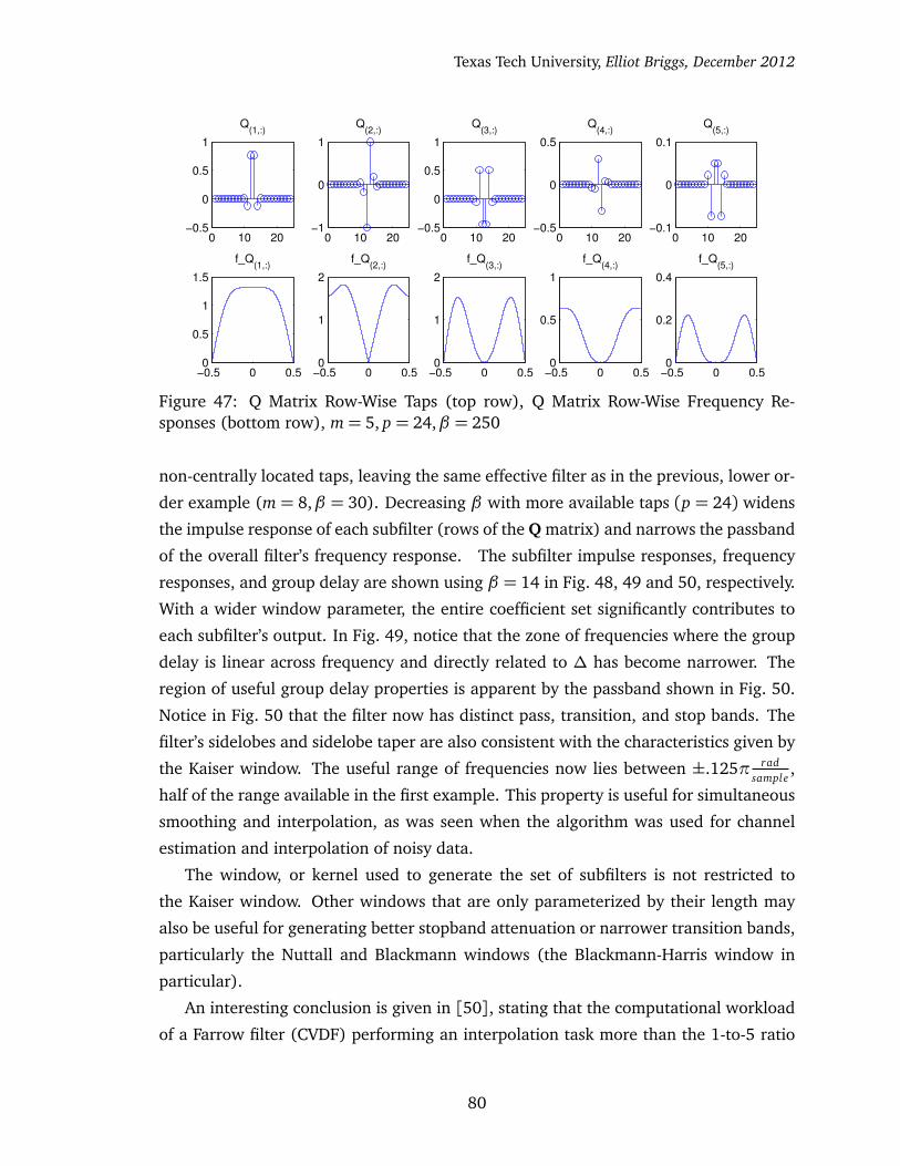
Texas Tech University, Elliot Briggs, December 2012
0 10 20−0.5
0
0.5
1
Q(1,:)
0 10 20−1
0
1
Q(2,:)
0 10 20−0.5
0
0.5
1
Q(3,:)
0 10 20−0.5
0
0.5
Q(4,:)
0 10 20−0.1
0
0.1
Q(5,:)
−0.5 0 0.50
0.5
1
1.5
f_Q(1,:)
−0.5 0 0.50
1
2
f_Q(2,:)
−0.5 0 0.50
1
2
f_Q(3,:)
−0.5 0 0.50
0.5
1
f_Q(4,:)
−0.5 0 0.50
0.2
0.4
f_Q(5,:)
Figure 47: Q Matrix Row-Wise Taps (top row), Q Matrix Row-Wise Frequency Re-sponses (bottom row), m= 5, p = 24,β = 250
non-centrally located taps, leaving the same effective filter as in the previous, lower or-
der example (m = 8,β = 30). Decreasing β with more available taps (p = 24) widens
the impulse response of each subfilter (rows of the Q matrix) and narrows the passband
of the overall filter’s frequency response. The subfilter impulse responses, frequency
responses, and group delay are shown using β = 14 in Fig. 48, 49 and 50, respectively.
With a wider window parameter, the entire coefficient set significantly contributes to
each subfilter’s output. In Fig. 49, notice that the zone of frequencies where the group
delay is linear across frequency and directly related to ∆ has become narrower. The
region of useful group delay properties is apparent by the passband shown in Fig. 50.
Notice in Fig. 50 that the filter now has distinct pass, transition, and stop bands. The
filter’s sidelobes and sidelobe taper are also consistent with the characteristics given by
the Kaiser window. The useful range of frequencies now lies between ±.125π radsample
,
half of the range available in the first example. This property is useful for simultaneous
smoothing and interpolation, as was seen when the algorithm was used for channel
estimation and interpolation of noisy data.
The window, or kernel used to generate the set of subfilters is not restricted to
the Kaiser window. Other windows that are only parameterized by their length may
also be useful for generating better stopband attenuation or narrower transition bands,
particularly the Nuttall and Blackmann windows (the Blackmann-Harris window in
particular).
An interesting conclusion is given in [50], stating that the computational workload
of a Farrow filter (CVDF) performing an interpolation task more than the 1-to-5 ratio
80

Texas Tech University, Elliot Briggs, December 2012
0 10 20−0.5
0
0.5
1
Q(1,:)
0 10 20−0.4
−0.2
0
0.2
0.4
Q(2,:)
0 10 20−0.1
−0.05
0
0.05
0.1
Q(3,:)
0 10 20−5
0
5x 10
−3Q(4,:)
0 10 20−1
−0.5
0
0.5
1x 10
−3Q(5,:)
−0.5 0 0.50
1
2
3
4
5
f_Q(1,:)
−0.5 0 0.50
0.5
1
1.5
f_Q(2,:)
−0.5 0 0.50
0.1
0.2
0.3
0.4
0.5
f_Q(3,:)
−0.5 0 0.50
0.01
0.02
0.03
0.04
f_Q(4,:)
−0.5 0 0.50
2
4
6x 10
−3f_Q(5,:)
Figure 48: Q Matrix Row-Wise Taps (top row), Q Matrix Row-Wise Frequency Re-sponses (bottom row), m= 5, p = 24,β = 14
−1 −0.8 −0.6 −0.4 −0.2 0 0.2 0.4 0.6 0.8
11.5
12
12.5
13
13.5
Normalized Frequency (×π rad/sample)
Gro
up
de
lay (
in s
am
ple
s)
Group Delay: Kaiser Window Kernal, p=24, m=5, β=14
∆=−1
∆=−.75
∆=−.5
∆=−.25
∆=0
∆=.25
∆=.5
∆=.75
∆=1
Figure 49: Generated CVFD (Farrow) Filter’s Group Delay vs. ∆: m= 5, p = 24,β = 14
81

Texas Tech University, Elliot Briggs, December 2012
−1 −0.8 −0.6 −0.4 −0.2 0 0.2 0.4 0.6 0.8
−120
−100
−80
−60
−40
−20
0
Normalized Frequency (×π rad/sample)
Magnitude (
dB
) (n
orm
aliz
ed to 0
dB
)
Magnitude (dB) and Phase Response: Kaiser Window Kernal, p=24, m=5, β=14
Figure 50: Generated CVFD (Farrow) Filter’s Magnitude vs. ∆: m = 5, p = 24,β = 14,Useful for Simultaneous Interpolation and Smoothing
results in fewer computations than the traditional polyphase implementation. This con-
clusion is intuitive because the filter has m = 5 arms, as does a comparable polyphase
upsampler; therefore any resampling ratio greater than 1-to-m or m-to-1 yields com-
putational benefits.
Perhaps the most attractive capability of this class of filters is the ability to per-
form irrational-ratio or “inconvenient-ratio” resampling tasks. A good example of
inconvenient-ratio resampling can be found when simulating a multi-path fading chan-
nel in software. Many channel models specify 5 or 10 ns tap delay resolution, implying
a 200 or 100 MHz sampling rate, respectively. However, to use the specified models,
the standard UMTS (i.e. LTE) sampling rates are multiples of 30.72 MHz and must be
resampled to match the channel model’s rate.
To perform resampling, the delay of the filter is continuously varied so the appro-
priate interpolated points are produced according to the desired resampling ratio. The
CVDF can be used to arbitrarily increase or decrease the sampling rate with arbitrary
phase shift. Fig. 51 shows the sidelobes produced when the input signal is oversampled
by varying degrees (indicated by N) and upsampled by 8 by decreasing ∆ by 1/8 for
each successive output sample, rolling over back around 1 upon underflowing below
0. The CVDF produces significant nulls located in the center of each spectral duplicate.
82

Texas Tech University, Elliot Briggs, December 2012
−1 −0.8 −0.6 −0.4 −0.2 0 0.2 0.4 0.6 0.8−150
−100
−50
0
Normalized Frequency (×π rad/sample)
Ma
gn
itu
de
(d
B)
(no
rma
lize
d t
o 0
dB
)
CVDF Resampler − Magnitude Response (dB) vs. Input Oversampledness − 1−to−8 upsampling
N=1
N=2
N=4
N=8
Figure 51: Sidelobes Resulting from CVFD Rate Transition with Varying Levels of InputOversampledness
�
m= 5, p = 8,β = 30�
Increasingly narrow spectral duplicates are increasingly attenuated by the nulls. The
oversampledness of the filter’s input determines the cascaded stop-band performance.
To achieve the generally desirable -96 dB stopband attenuation (or close to it), the
input signal must be oversampled by at least a factor of 8. The -96 dB stop-band repre-
sents the theoretical quantization noise floor for signals with 16-bit precision. This level
of precision is higher than what is effectively achieved by most realistic data converters,
assuring the converter is likely to be the limiting factor in the system.
Fig. 52 illustrates the structure of a generalized Farrow-based arbitrary-ratio upsam-
pler. If the input signal is oversampled, the design can be considered to be an arbitrary-
ratio resampler rather than an upsampler. The input is fed into a 8x polyphase upsam-
pling preprocessing filter, which provides the minimum necessary oversampledness to
achieve desirable stopband performance, even for nearly critically sampled input sig-
nals. The 8x prototype filter is assumed to be “non-ideal” and thus has a finite-width
transition band; hence the input signal can be “nearly” critically sampled, depending
on the prototype filter’s design characteristics. After the preprocessing step, the signal
is sent to the Farrow structure. The only updates to the Farrow structure from Fig. 43
83
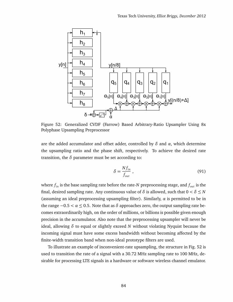
Texas Tech University, Elliot Briggs, December 2012
y[(n/8)+Δ]
q4
Ɵ4[n]
q3
Ɵ3[n]
q2
Ɵ2[n]
q1
Ɵ1[n]
q5
Ɵ5[n]
y[n/8]
h2
h3
h4
h5
h6
h7
h8
h1
y[n]
Δ- z-1δ α
Figure 52: Generalized CVDF (Farrow) Based Arbitrary-Ratio Upsampler Using 8xPolyphase Upsampling Preprocessor
are the added accumulator and offset adder, controlled by δ and α, which determine
the upsampling ratio and the phase shift, respectively. To achieve the desired rate
transition, the δ parameter must be set according to:
δ =N fin
fout, (91)
where fin is the base sampling rate before the rate-N preprocessing stage, and fout is the
final, desired sampling rate. Any continuous value of δ is allowed, such that 0< δ ≤ N
(assuming an ideal preprocessing upsampling filter). Similarly, α is permitted to be in
the range−0.5< α≤ 0.5. Note that as δ approaches zero, the output sampling rate be-
comes extraordinarily high, on the order of millions, or billions is possible given enough
precision in the accumulator. Also note that the preprocessing upsampler will never be
ideal, allowing δ to equal or slightly exceed N without violating Nyquist because the
incoming signal must have some excess bandwidth without becoming affected by the
finite-width transition band when non-ideal prototype filters are used.
To illustrate an example of inconvenient-rate upsampling, the structure in Fig. 52 is
used to transition the rate of a signal with a 30.72 MHz sampling rate to 100 MHz, de-
sirable for processing LTE signals in a hardware or software wireless channel emulator.
84
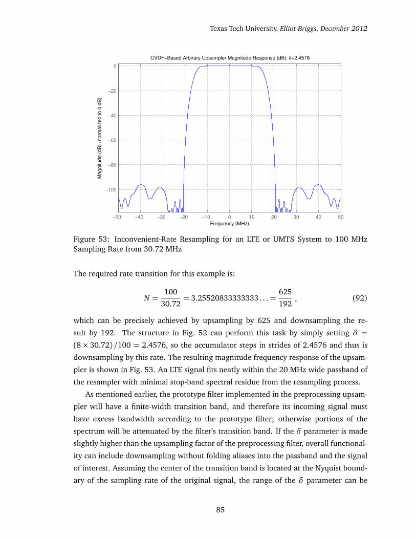
Texas Tech University, Elliot Briggs, December 2012
−50 −40 −30 −20 −10 0 10 20 30 40 50
−100
−80
−60
−40
−20
0
Frequency (MHz)
Magnitude (
dB
) (n
orm
aliz
ed to 0
dB
)
CVDF−Based Arbirary Upsampler Magnitude Response (dB): δ=2.4576
Figure 53: Inconvenient-Rate Resampling for an LTE or UMTS System to 100 MHzSampling Rate from 30.72 MHz
The required rate transition for this example is:
N =100
30.72= 3.25520833333333 . . .=
625
192, (92)
which can be precisely achieved by upsampling by 625 and downsampling the re-
sult by 192. The structure in Fig. 52 can perform this task by simply setting δ =
(8× 30.72)/100 = 2.4576, so the accumulator steps in strides of 2.4576 and thus is
downsampling by this rate. The resulting magnitude frequency response of the upsam-
pler is shown in Fig. 53. An LTE signal fits neatly within the 20 MHz wide passband of
the resampler with minimal stop-band spectral residue from the resampling process.
As mentioned earlier, the prototype filter implemented in the preprocessing upsam-
pler will have a finite-width transition band, and therefore its incoming signal must
have excess bandwidth according to the prototype filter; otherwise portions of the
spectrum will be attenuated by the filter’s transition band. If the δ parameter is made
slightly higher than the upsampling factor of the preprocessing filter, overall functional-
ity can include downsampling without folding aliases into the passband and the signal
of interest. Assuming the center of the transition band is located at the Nyquist bound-
ary of the sampling rate of the original signal, the range of the δ parameter can be
85

Texas Tech University, Elliot Briggs, December 2012
−15 −10 −5 0 5 10 15
−1
−0.8
−0.6
−0.4
−0.2
0
Frequency (MHz)
Ma
gn
itu
de
(d
B)
(no
rma
lize
d t
o 0
dB
)
CVDF (Farrow)−Based Resampler Magnitude Response (dB): N=8, δ=8.17, α=.35
Figure 54: Farrow-Based LTE Resampling Filter
extended to 0 < δ <�
N + α
2
�
without overlapping aliases, where α in this context
denotes the excess bandwidth of the preprocessing filter and thus the input signal.
Using δ = 8.17 and configuring the preprocessing prototype filter’s excess band-
width using α = .35, the result in Fig. 54 shows minimal interference from aliases in
the passband. The overall downsampling factor in this example is 8/8.17 ∼= 0.9791,
and the system is able to recover LTE signals with sampling clock errors of just over
+2%. This capability is a critical component to the architecture illustrated in Fig. 7 and
introduced in Sec. 3.3, where the incoming signal is dynamically resampled to cancel
sampling clock frequency errors based on time-domain estimates.
86

Texas Tech University, Elliot Briggs, December 2012
6 Exploitation of Excess Cyclic Prefix to Improve Reception Quality
As described in Sec. 3.2, ISI is introduced when the DFT operation contains energy from
more than one symbol. Orthogonal reception is maintained when the starting point of
the symbol position lies in the segment of CP after the echoes from the previous symbol
have subsided (Eq. 86). Echoes are introduced by a channel with “memory”. The size
of unusable CP is determined by the channel’s excess delay, denoted by d.
In a system operating in a memoryless channel (i.e. d = 0), no ISI energy is present
and the entire CP is redundant. In a channel with memory, the first segment of d
samples in the CP are corrupted by ISI, leaving L− d excess CP samples. It is assumed
that an OFDM system operating in its intended channel environment will be designed
with an adequately long CP to provide ISI-free operation in normal circumstances.
Therefore, in normal circumstances, the CP is longer than is required by the channel
and the received signal contains redundancy.
The LTE standard includes two CP modes, “normal” and “extended”, with a dura-
tion of 4.6875 µs and 16.666 µs, respectively. Out of the three channels used in the
LTE conformance tests, the longest excess delay is 5 µs in the extended typical urban
scenario [42], leaving inadequate CP for the “normal” mode and vast lengths of un-
used, excess CP for the extended mode. Considering the RS configuration, highlighted
by Sec. 4.3, the frequency spacing of the RSs introduces downsampling of the channel’s
frequency response, limiting the maximum excess delay to a value far shorter than the
entire CP duration, thereby implying that not only does normal operation imply CP
redundancy, but very large amounts of it. The LTE RS configuration can resolve excess
delays and symbol timing shifts of up to M/2q samples, or 5.555 µs (Eq. 86). Assum-
ing no symbol timing shift while operating in the extended CP mode, at least 2/3 of
the CP is redundant under typical conditions.
Palenik in [53] likens the excess CP as an inner repetition channel code, while
the added turbo or low-density parity check (LDPC) channel coding is the outer code.
Palenik combines the redundant information after demodulation and demapping by
summing the semi-correlated set of log-likelihood ratios computed by separate soft-
decision demappers. Performing redundancy combination after equalization, demod-
ulation, and demapping dramatically increases the computational complexity of the
receiver and fails to benefit receiver components that could take advantage of the
available redundancy, such as the channel estimation component, which primarily in-
fluences overall receiver performance.
Nearly every OFDM receiver must be capable of performing channel estimation and
87

Texas Tech University, Elliot Briggs, December 2012
equalization, a process that requires the capablility of estimating the (inverse of) the
channel’s frequency and/or impulse response. In all cases, an estimate of d is either
directly, or readily available, which can be used to estimate the available number of re-
dundant CP samples. Many existing channel estimation algorithms take the channel’s
observed noisy frequency response, convert it to the CIR on which statistical estima-
tion is performed, then convert the result back to the frequency response for equaliza-
tion [32,54,55]. Through the process of converting the frequency response to the CIR,
an estimate of d can be easily gleaned from the already existing information.
First, an inefficient but intuitive method to utilize the available redundancy requires
a slight modification of the existing OFDM receiver by adding a second DFT operation.
One DFT operates on the block of M contiguous samples starting at m = −(L − d) +
1, and the other starts at m = 0. The DFT starting at m = −(L − d) + 1 is offset
by a known amount from the other, and the channel estimation component is not
needed to derotate its phase. Phase correction (pre-equalization) can be performed by
multiplying the DFT result with ΦH .
ΦH = diag�
φH , (93)
where φ is the M × 1 vector defined in Eq. 6 using τ = −m. The timing offset be-
tween the DFT operations is known and the RSs are not needed to determine the phase
rotation. In this case, the timing shift can extend beyond the frequency resolution lim-
itation imposed by the RS frequency spacing. After equalizing the phase of the offset
DFT, the DFT results can be summed to form a single vector. After the summation,
the signal and noise power are not scaled equally. The signal power is doubled, and
the noise power increase is dependent on the level of correlation between the additive
noise residing in the samples used in the pair of DFT operations. The correlation is di-
rectly dependent on the time separation of the two DFT windows. When the two DFT
windows contain exactly the same samples, the noise terms are equal and maximally
correlated. Conversely, if the DFT windows are maximally separated, the number of
mutually exclusive observations of the signal obtained by each DFT operation are maxi-
mized, thus minimizing the level of correlation in the noise. The receiver that combines
88

Texas Tech University, Elliot Briggs, December 2012
the redundancy in the available excess CP using two DFT operations is defined by
u(k) = HZT WHMx(k) + n(k)
v1(k) =WMZRu(k)
v2(k) = ΦHmWMZmu(k)
v(k) = E�
1
2
�
v1(k) + v2(k)�
�
,
(94)
where the new permuation matrix Zm is used to select any contiguous group of samples
in u(k) starting at postion m=−(L− d).
Zm =
0d
0IM
0L−d
0
(95)
A simpler, more computationally efficient method exists. Rather than performing
two DFT operations, the redundancy can be captured in the time domain. The re-
dundant samples can be directly summed together before the receiver’s DFT operation.
Assuming the noise is i.i.d throughout the entire symbol, the noise contained in each
redundant segment of symbol is uncorrelated. Summing the two segments in the time
domain reduces the relative noise variance while only requiring a single DFT opera-
tion. The time-domain combination is most effective when sampling frequency error
has been minimized or eliminated. The matrix notation representation of this receiver
is defined by
u(k) = HZT WHMx(k) + n(k)
v(k) = EWM
�
Z1+1
2
�
Z2+ Z3
�
�
u(k) ,(96)
where the M × P dimension permutation matrices are defined by
Z1 =
0L IM−L−d 0L−d
0 0 0
Z2 =
0 0
0 IL−d
Z3 =
0 0
0d IL−d0M
(97)
89
Texas Tech University, Elliot Briggs, December 2012
Z1 selects the first M − L− d samples after the CP, Z2 selects the final L− d samples in
u(k) and places zeros elsewhere, and Z3 selects the L − d samples before the CP and
shifts them to the end of a vector of zeros.
The redundant segments summed in Eq. 96 contain i.i.d. WGN from the n(k) vector.
Prior to the DFT operation, two levels of noise variance are present in the symbol
vector, resulting from the redundancy combination. The first M − L − d samples are
unaffected by the operation, having the baseline noise variance σ2n. However, the last
L − d samples now have an expected noise variance ofσ2
n
2. The two segments of noise
in each symbol are uncorrelated; therefore the noise variances of each segment can be
summed to determine the joint variance.
σ2n =
σ2n
M − L− d+
1
2
σ2n
L− d(98)
According to the Parseval/Rayleigh energy conservation theorem, the noise power re-
mains constant before and after the DFT, therefore by combining the excess CP samples,
the noise variance is reduced by a level that depends on the channel’s excess delay and
the relative size of the CP to the DFT size.
After combining the redundancy, a level of correlation is introduced to the noise
across the frequency bins of the DFT, which is straightforward to prove. The noise
profile can be represented using the rectangle, or “rect” function and its discrete-time
Fourier transform as defined by
rect� n
M
�
=
1,�
�
�
nM
�
�
�≤ 12
0, otherwise
DT F T←→sin�
ω�
M + 12
��
sin�
ω
2
� . (99)
and, using the comb function
combM (n) =+∞∑
k=−∞
δ (n− kM)DT F T←→
1
M
+∞∑
k=−∞
δ
�
ω
2π−
k
M
�
=+∞∑
k=−∞
e− jωMk (100)
to periodically profile a discrete-time unit-variance zero-mean Gaussian random vari-
able n (n)
�
σ2
2
�
rect� n
M − d
�
+ 1�
⊗ combM
�
n−M − d
2
�
�
× n (n) , (101)
where ⊗ denotes the discrete convolution operator and σ2n denotes the variance of the
90
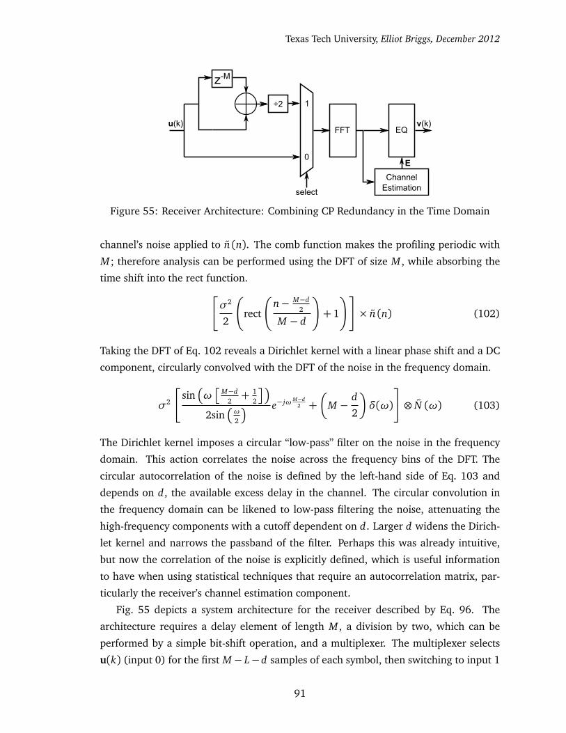
Texas Tech University, Elliot Briggs, December 2012
z-M
÷2
u(k)FFT
v(k)
ChannelEstimationselect
0
1
EQ
E
Figure 55: Receiver Architecture: Combining CP Redundancy in the Time Domain
channel’s noise applied to n (n). The comb function makes the profiling periodic with
M ; therefore analysis can be performed using the DFT of size M , while absorbing the
time shift into the rect function.
σ2
2
rect
n− M−d2
M − d
!
+ 1
!
× n (n) (102)
Taking the DFT of Eq. 102 reveals a Dirichlet kernel with a linear phase shift and a DC
component, circularly convolved with the DFT of the noise in the frequency domain.
σ2
sin�
ω�
M−d2+ 1
2
��
2sin�
ω
2
� e− jω M−d2 +
�
M −d
2
�
δ(ω)
⊗ N (ω) (103)
The Dirichlet kernel imposes a circular “low-pass” filter on the noise in the frequency
domain. This action correlates the noise across the frequency bins of the DFT. The
circular autocorrelation of the noise is defined by the left-hand side of Eq. 103 and
depends on d, the available excess delay in the channel. The circular convolution in
the frequency domain can be likened to low-pass filtering the noise, attenuating the
high-frequency components with a cutoff dependent on d. Larger d widens the Dirich-
let kernel and narrows the passband of the filter. Perhaps this was already intuitive,
but now the correlation of the noise is explicitly defined, which is useful information
to have when using statistical techniques that require an autocorrelation matrix, par-
ticularly the receiver’s channel estimation component.
Fig. 55 depicts a system architecture for the receiver described by Eq. 96. The
architecture requires a delay element of length M , a division by two, which can be
performed by a simple bit-shift operation, and a multiplexer. The multiplexer selects
u(k) (input 0) for the first M− L−d samples of each symbol, then switching to input 1
91
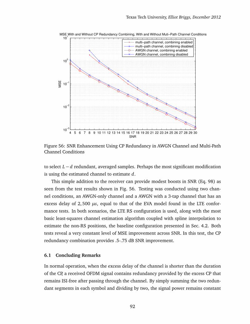
Texas Tech University, Elliot Briggs, December 2012
4 5 6 7 8 9 10 11 12 13 14 15 16 17 18 19 20 21 22 23 24 25 26 27 28 29 3010
−3
10−2
10−1
100
101
SNR
MS
E
MSE With and Without CP Redundancy Combining, With and Without Muti−Path Channel Conditions
multi−path channel, combining enabled
multi−path channel, combining disabled
AWGN channel, combining enabled
AWGN channel, combining disabled
Figure 56: SNR Enhancement Using CP Redundancy in AWGN Channel and Multi-PathChannel Conditions
to select L−d redundant, averaged samples. Perhaps the most significant modification
is using the estimated channel to estimate d.
This simple addition to the receiver can provide modest boosts in SNR (Eq. 98) as
seen from the test results shown in Fig. 56. Testing was conducted using two chan-
nel conditions, an AWGN-only channel and a AWGN with a 3-tap channel that has an
excess delay of 2, 500 µs, equal to that of the EVA model found in the LTE confor-
mance tests. In both scenarios, the LTE RS configuration is used, along with the most
basic least-squares channel estimation algorithm coupled with spline interpolation to
estimate the non-RS positions, the baseline configuration presented in Sec. 4.2. Both
tests reveal a very constant level of MSE improvement across SNR. In this test, the CP
redundancy combination provides .5-.75 dB SNR improvement.
6.1 Concluding Remarks
In normal operation, when the excess delay of the channel is shorter than the duration
of the CP, a received OFDM signal contains redundancy provided by the excess CP that
remains ISI-free after passing through the channel. By simply summing the two redun-
dant segments in each symbol and dividing by two, the signal power remains constant
92
Texas Tech University, Elliot Briggs, December 2012
while the noise variance is reduced by a factor of 2. In an LTE system operating in nor-
mal conditions, CP redundancy is guaranteed. Assuming normal operating conditions,
at least 2/3 of the CP is redundant in the extended CP configuration. The overall SNR
gain achieved by the redundancy combination has been shown to be significant, given
its simplicity. The SNR gain is obtained using an estimate of the channel’s excess delay,
information that is already available or easily obtained from the channel estimation
component in the receiver.
93

Texas Tech University, Elliot Briggs, December 2012
7 Real-Time Wireless Channel Emulation
To test algorithms in a wireless communications system, the designer may first perform
simplistic simulations using a time-stationary AWGN channel. Later, more complex
simulations with time-varying channel conditions must be performed that take into
account the channel conditions in the intended operating environment. To perform
time-varying channel simulations, recorded channel conditions could be used, or even
live field testing could be performed. These methods constrain the simulation to a
specific operating environment, may not be repeatable, and may be cost prohibitive.
Instead, if the channel can be modeled, computer simulation can be performed with
user-defined channel properties that emulate real-world conditions. The user can pro-
gram the emulator with industry standard models, or even their own models derived
from empirical measurements in their desired scenario.
Using computer software, short simulations of time-varying channels can be per-
formed with relatively little effort. Computer simulation is rarely performed in real-
time and is not suitable for use with a communications system that has already been
implemented in real-time hardware. Real-time hardware tests are an essential part of
system development. It is typical for a designer to discover new or unforeseen problems
when their implementation is exposed to real-world or real-time conditions, particu-
larly involving complex state machines or control systems embedded in the receiver
architecture.
It has become common to generate and store pre-computed simulated signals or
recorded field test signals in large banks of DRAM or disk storage. The stored signal
is then “played” by streaming the samples to a DAC in real-time. For long simulations,
the signal must either repeat without cyclic continuity, or must end. When channel
conditions are repeated, a large instantaneous discontinuity occurs. Not only are the
discontinuities unrealistic, but can cause unexpected problems. The abrupt repetition
boundaries can cause spurious spectral emissions, or can even cause internal receiver
control systems and adaptive algorithms to fail or perform unexpectedly. Even if the
channel conditions do have continuous repetition boundaries, the receiver experiences
the same repeating scenario, which may give the designer the false illusion and confi-
dence in the receiver’s general behavior.
For continuous, long-term testing of hardware receivers in real-time, a hardware
channel emulator becomes necessary, capable of processing signals in real-time. The
transmitted signal is generated and stored in RAM but can be repeated with cyclic
continuity at the symbol boundaries. For simulation with an LTE system, several frames
94
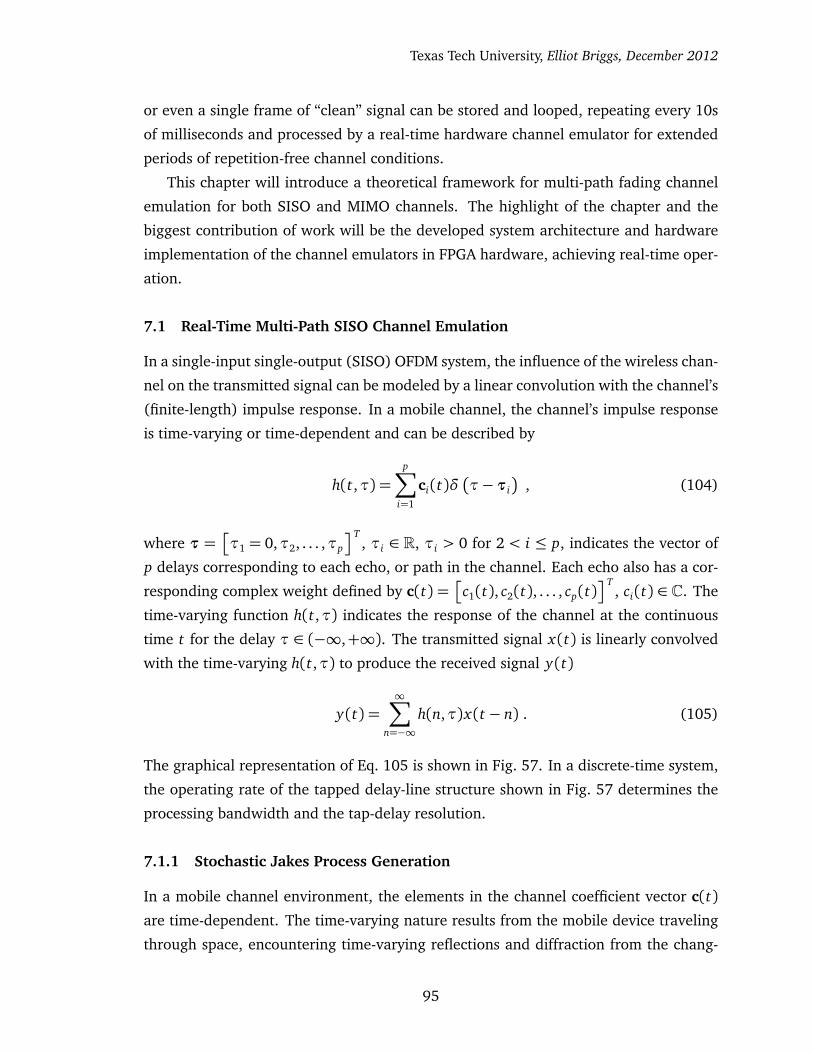
Texas Tech University, Elliot Briggs, December 2012
or even a single frame of “clean” signal can be stored and looped, repeating every 10s
of milliseconds and processed by a real-time hardware channel emulator for extended
periods of repetition-free channel conditions.
This chapter will introduce a theoretical framework for multi-path fading channel
emulation for both SISO and MIMO channels. The highlight of the chapter and the
biggest contribution of work will be the developed system architecture and hardware
implementation of the channel emulators in FPGA hardware, achieving real-time oper-
ation.
7.1 Real-Time Multi-Path SISO Channel Emulation
In a single-input single-output (SISO) OFDM system, the influence of the wireless chan-
nel on the transmitted signal can be modeled by a linear convolution with the channel’s
(finite-length) impulse response. In a mobile channel, the channel’s impulse response
is time-varying or time-dependent and can be described by
h(t,τ) =p∑
i=1
ci(t)δ�
τ−τi�
, (104)
where τ =�
τ1 = 0,τ2, . . . ,τp
�T, τi ∈ R, τi > 0 for 2 < i ≤ p, indicates the vector of
p delays corresponding to each echo, or path in the channel. Each echo also has a cor-
responding complex weight defined by c(t) =�
c1(t), c2(t), . . . , cp(t)�T
, ci(t) ∈ C. The
time-varying function h(t,τ) indicates the response of the channel at the continuous
time t for the delay τ ∈ (−∞,+∞). The transmitted signal x(t) is linearly convolved
with the time-varying h(t,τ) to produce the received signal y(t)
y(t) =∞∑
n=−∞h(n,τ)x(t − n) . (105)
The graphical representation of Eq. 105 is shown in Fig. 57. In a discrete-time system,
the operating rate of the tapped delay-line structure shown in Fig. 57 determines the
processing bandwidth and the tap-delay resolution.
7.1.1 Stochastic Jakes Process Generation
In a mobile channel environment, the elements in the channel coefficient vector c(t)
are time-dependent. The time-varying nature results from the mobile device traveling
through space, encountering time-varying reflections and diffraction from the chang-
95
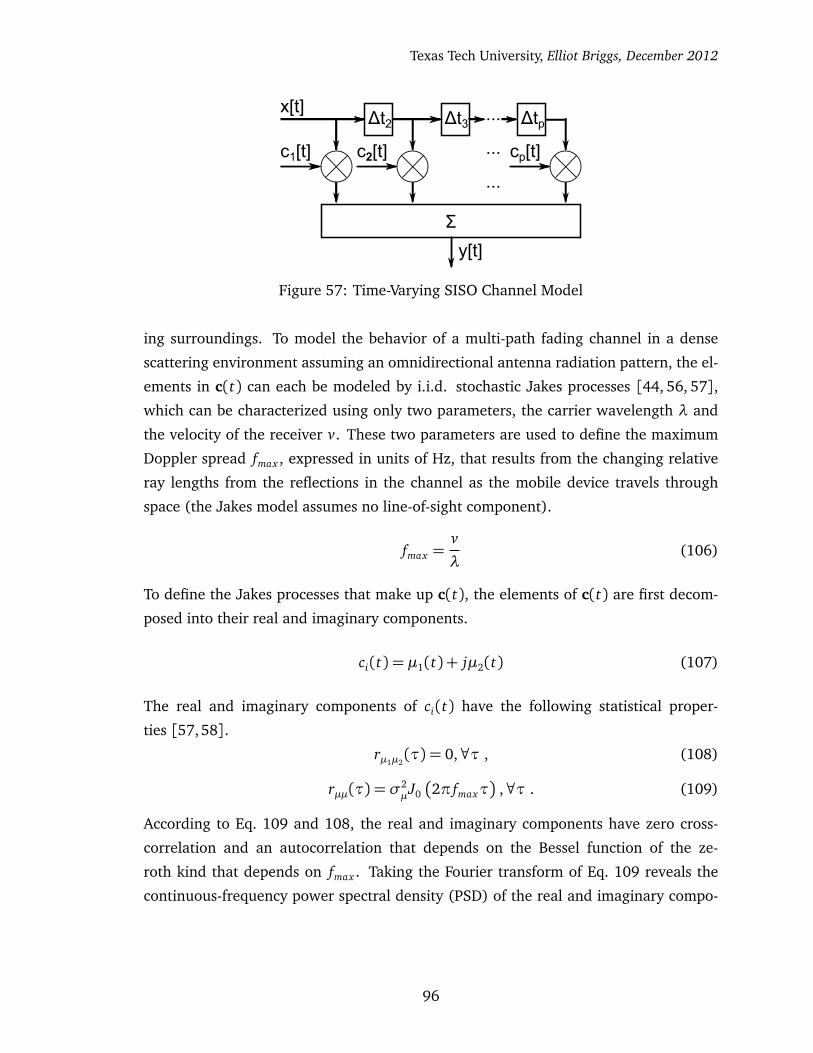
Texas Tech University, Elliot Briggs, December 2012
x[t]Δt2
c1[t]
Δt3
c2[t]
Δtp...
cp[t]...
...
Σ
y[t]
Figure 57: Time-Varying SISO Channel Model
ing surroundings. To model the behavior of a multi-path fading channel in a dense
scattering environment assuming an omnidirectional antenna radiation pattern, the el-
ements in c(t) can each be modeled by i.i.d. stochastic Jakes processes [44, 56, 57],
which can be characterized using only two parameters, the carrier wavelength λ and
the velocity of the receiver v. These two parameters are used to define the maximum
Doppler spread fmax , expressed in units of Hz, that results from the changing relative
ray lengths from the reflections in the channel as the mobile device travels through
space (the Jakes model assumes no line-of-sight component).
fmax =v
λ(106)
To define the Jakes processes that make up c(t), the elements of c(t) are first decom-
posed into their real and imaginary components.
ci(t) = µ1(t) + jµ2(t) (107)
The real and imaginary components of ci(t) have the following statistical proper-
ties [57,58].
rµ1µ2(τ) = 0,∀τ , (108)
rµµ(τ) = σ2µJ0
�
2π fmaxτ�
,∀τ . (109)
According to Eq. 109 and 108, the real and imaginary components have zero cross-
correlation and an autocorrelation that depends on the Bessel function of the ze-
roth kind that depends on fmax . Taking the Fourier transform of Eq. 109 reveals the
continuous-frequency power spectral density (PSD) of the real and imaginary compo-
96
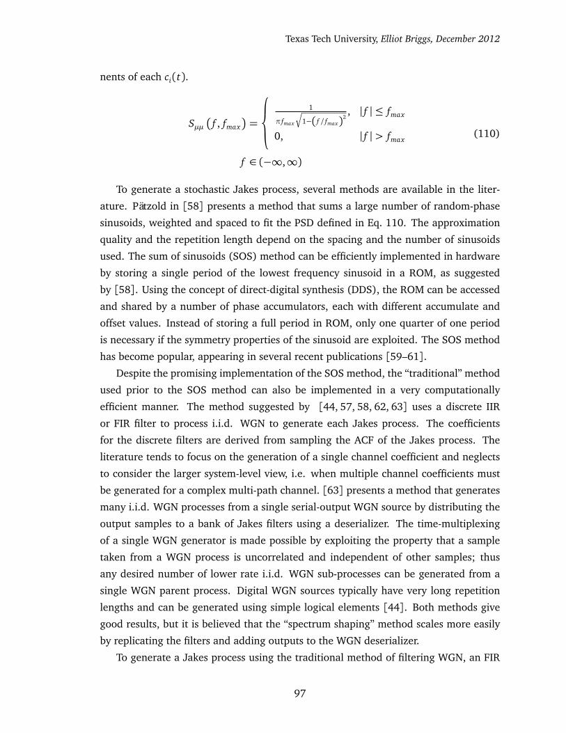
Texas Tech University, Elliot Briggs, December 2012
nents of each ci(t).
Sµµ�
f , fmax�
=
1
π fmax
q
1−( f / fmax)2, | f | ≤ fmax
0, | f |> fmax
f ∈ (−∞,∞)
(110)
To generate a stochastic Jakes process, several methods are available in the liter-
ature. Pätzold in [58] presents a method that sums a large number of random-phase
sinusoids, weighted and spaced to fit the PSD defined in Eq. 110. The approximation
quality and the repetition length depend on the spacing and the number of sinusoids
used. The sum of sinusoids (SOS) method can be efficiently implemented in hardware
by storing a single period of the lowest frequency sinusoid in a ROM, as suggested
by [58]. Using the concept of direct-digital synthesis (DDS), the ROM can be accessed
and shared by a number of phase accumulators, each with different accumulate and
offset values. Instead of storing a full period in ROM, only one quarter of one period
is necessary if the symmetry properties of the sinusoid are exploited. The SOS method
has become popular, appearing in several recent publications [59–61].
Despite the promising implementation of the SOS method, the “traditional” method
used prior to the SOS method can also be implemented in a very computationally
efficient manner. The method suggested by [44, 57, 58, 62, 63] uses a discrete IIR
or FIR filter to process i.i.d. WGN to generate each Jakes process. The coefficients
for the discrete filters are derived from sampling the ACF of the Jakes process. The
literature tends to focus on the generation of a single channel coefficient and neglects
to consider the larger system-level view, i.e. when multiple channel coefficients must
be generated for a complex multi-path channel. [63] presents a method that generates
many i.i.d. WGN processes from a single serial-output WGN source by distributing the
output samples to a bank of Jakes filters using a deserializer. The time-multiplexing
of a single WGN generator is made possible by exploiting the property that a sample
taken from a WGN process is uncorrelated and independent of other samples; thus
any desired number of lower rate i.i.d. WGN sub-processes can be generated from a
single WGN parent process. Digital WGN sources typically have very long repetition
lengths and can be generated using simple logical elements [44]. Both methods give
good results, but it is believed that the “spectrum shaping” method scales more easily
by replicating the filters and adding outputs to the WGN deserializer.
To generate a Jakes process using the traditional method of filtering WGN, an FIR
97

Texas Tech University, Elliot Briggs, December 2012
−1 −0.8 −0.6 −0.4 −0.2 0 0.2 0.4 0.6 0.8 1−100
−80
−60
−40
−20
0
norm
aliz
ed m
agnitude (
dB
)
normalized frequency (× fs)
frequency response of designed jakes filter, fd=.8, N=256
Pre−Window
Post−Window
16 32 48 64 80 96 112 128 144 160 176 192 208 224 240 256−0.2
0
0.2
0.4
0.6
0.8
1
norm
aliz
ed a
mplit
ude
samples
impulse response
Pre−Window
Post−Window
Figure 58: Designed Jakes FIR Filter: NJakes = 256, fmax = 100 Hz, fd = .8
filter can be generated by sampling the PSD given by Eq. 110.
H( fk) =Æ
Sµµ�
fk, fd�
,
fk =k− 1
NJakes−
1
2,
k = 1, 2, . . . , NJakes ,
fd =2 fmax
fs.
(111)
Here, NJakes represents the number of taps used in the FIR filter, fs indicates the sam-
pling frequency, and fd defines the Doppler spread normalized to the sampling fre-
quency. After sampling the PSD, a Kaiser window is used on the Fourier transform
of H( fk) to obtain the set of FIR filter coefficients. To establish a running design ex-
ample, the following parameters will be chosen; p = 9, fmax = 100 Hz, fd = .8, and
NJakes = 256. Using these parameters and Eq. 111, Fig. 58 shows the designed Jakes
FIR filter. Before windowing, the filter’s impulse response decays very slowly due to the
98
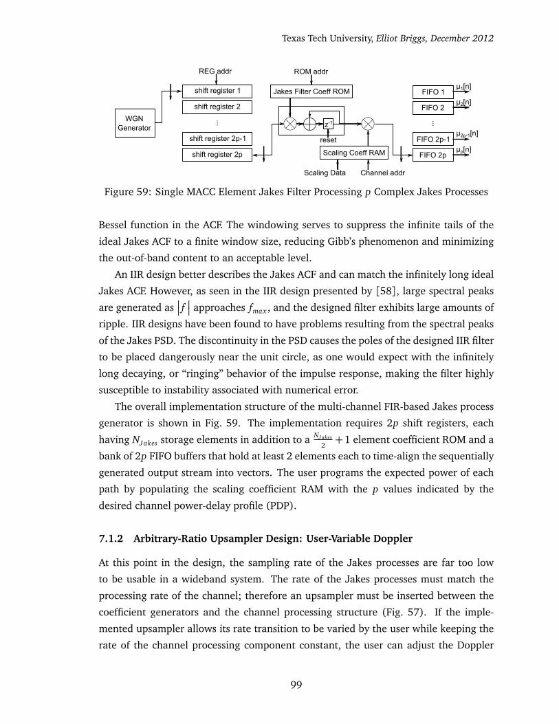
Texas Tech University, Elliot Briggs, December 2012
WGN Generator
...
shift register 2p-1
Jakes Filter Coeff ROM
...
FIFO 1
FIFO 2
FIFO 2p-1
FIFO 2p
shift register 1
shift register 2
shift register 2p
z-1
reset
µ1[n]
ROM addrREG addr
Scaling Coeff RAM
Channel addrScaling Data
µ2[n]
µ2p-1[n]
µp[n]
Figure 59: Single MACC Element Jakes Filter Processing p Complex Jakes Processes
Bessel function in the ACF. The windowing serves to suppress the infinite tails of the
ideal Jakes ACF to a finite window size, reducing Gibb’s phenomenon and minimizing
the out-of-band content to an acceptable level.
An IIR design better describes the Jakes ACF and can match the infinitely long ideal
Jakes ACF. However, as seen in the IIR design presented by [58], large spectral peaks
are generated as�
� f�
� approaches fmax , and the designed filter exhibits large amounts of
ripple. IIR designs have been found to have problems resulting from the spectral peaks
of the Jakes PSD. The discontinuity in the PSD causes the poles of the designed IIR filter
to be placed dangerously near the unit circle, as one would expect with the infinitely
long decaying, or “ringing” behavior of the impulse response, making the filter highly
susceptible to instability associated with numerical error.
The overall implementation structure of the multi-channel FIR-based Jakes process
generator is shown in Fig. 59. The implementation requires 2p shift registers, each
having NJakes storage elements in addition to a NJakes
2+1 element coefficient ROM and a
bank of 2p FIFO buffers that hold at least 2 elements each to time-align the sequentially
generated output stream into vectors. The user programs the expected power of each
path by populating the scaling coefficient RAM with the p values indicated by the
desired channel power-delay profile (PDP).
7.1.2 Arbitrary-Ratio Upsampler Design: User-Variable Doppler
At this point in the design, the sampling rate of the Jakes processes are far too low
to be usable in a wideband system. The rate of the Jakes processes must match the
processing rate of the channel; therefore an upsampler must be inserted between the
coefficient generators and the channel processing structure (Fig. 57). If the imple-
mented upsampler allows its rate transition to be varied by the user while keeping the
rate of the channel processing component constant, the user can adjust the Doppler
99

Texas Tech University, Elliot Briggs, December 2012
4x upsamplerPolyphaseFilter - y
PolyphaseFilter - y*
integer
δ
k
fraction
α
k
1-α
μ[n]
accumulator
μ[δn/128]
Figure 60: Arbitrary-Ratio Resampler Architecture
frequency fmax . The change in rate adds a variable amount of additional excess band-
width to the nearly critically sampled Jakes processes. This action also reduces the
workload of the Jakes process generators. Increasing (decreasing) the rate transition
slows (speeds) the consumption of the samples produced by the Jakes processes. The
variable rate upsampler paces (determines the rate of) the Jakes process generator.
To perform arbitrary-ratio upsampling, the design shown in Fig. 60, introduced
in [25, 64], as well as the resampling architecture presented in Fig. 52 can be used.
Both are capable of producing virtually limitless upsampling factors with near arbitrary
resolution that depends on their respective accumulator widths. Both designs require a
preprocessing upsampling stage to assure adequate stop-band performance. The dual
polyphase design is the slightly more attractive of the two with fewer components that
must operate at the full output rate. The Farrow-based design requires a long chain of
adders and multipliers that evaluate output polynomials at the full output rate of the
system. While the chain can be pipelined to achieve good speed performance, it would
still require more full-rate resources than the dual polyphase technique.
The dual polyphase design exploits the linear-time-variant nature of polyphase fil-
ters (and resamplers in general). A rate-N polyphase upsampler can produce N ver-
sions of its output, depending on where the commutator is located at a particular time
instant. The clever concept of this design is that, given two polyphase upsampling
filters that process the same input, two phases (versions of the output signal) can be
generated at the output by having one of the commutator arms lag the other in the
adjacent position. In this design, even if δ > 1 and the commutators hop and skip
locations, the two filters produce two adjacent phases in the phase space. The frac-
100

Texas Tech University, Elliot Briggs, December 2012
tional component of the accumulator is then used for linear interpolation between the
two polyphase filter outputs. The linear interpolation upsamples the output signal of
the polyphase upsamplers while attenuating the spectral duplicates that are generated.
The process is equivalent to upsampling the signal by a variable amount and convolving
the result with a variable-width triangle pulse. The Fourier transform of the triangle
pulse is a squared sinc that has its spectral nulls aligned with the spectral duplicates
produced by the upsampling. If the output of the polyphase upsampler is oversampled
by a large enough factor, the spectral duplicates will be narrow enough to allow most of
the unwanted spectral content to reside deep within each null of the squared sinc func-
tion. This concept was also seen in the design of the Farrow-based arbitrary upsampler
in Fig. 51. If the incoming signal is first oversampled by 4x, and proceeded by upsam-
pling by a factor of 32x using the dual polyphase structure, the spectral duplicates will
be narrow enough to be attenuated below the target -96 dB stopband target.
To design the arbitrary resampler, the two fixed-rate upsampling components are
designed for maximum efficiency. Several design options exist for the preprocessing
filter. A single-stage polyphase FIR structure requires a larger coefficient ROM than the
functionally similar upsampler that is split into cascaded stages of rate-2 components,
i.e. Fig. 21. This type of design uses half-band FIR filters, which only require one
quarter of their coefficients to be stored in ROM but may use more hardware multipliers
in an FPGA/ASIC implementation as a result of the split to two stages. Similar to the
previous option, the third option uses two stages of half-band polyphase IIR filters that
are designed for linear phase. The IIR filters are constructed for efficiency using all-
pass second-order sections, and are especially well-suited for software implementation.
The IIR design uses very few coefficients and has a very low workload.
The design of the filter will compare both FIR and IIR half-band designs. The over-
lay and cascaded response of the designed Jakes and resampling filters are shown in
Fig. 61. The two filters require 18 and 5 coefficients for the first and second stages,
respectively. The passband ripple of the cascaded response is 200 µdB using floating-
point coefficients, and the workload of the filter is only 5.75 MACCs/output.
Each 2x upsampling component in the cascade can be implemented using the struc-
ture shown in Fig. 62. The implementation structure exploits the half-band polyphase
structure, which has one of its polyphase arms collapsed to a delay-line. In the single
MACC implementation, the input shift register is doubly used as the delay-line for the
polyphase arm that contains only zero coefficients. The output MUX acts as a virtual
commutator, passing one element from the MACC operation and then a subsequent
element from the end of the input shift register.
101
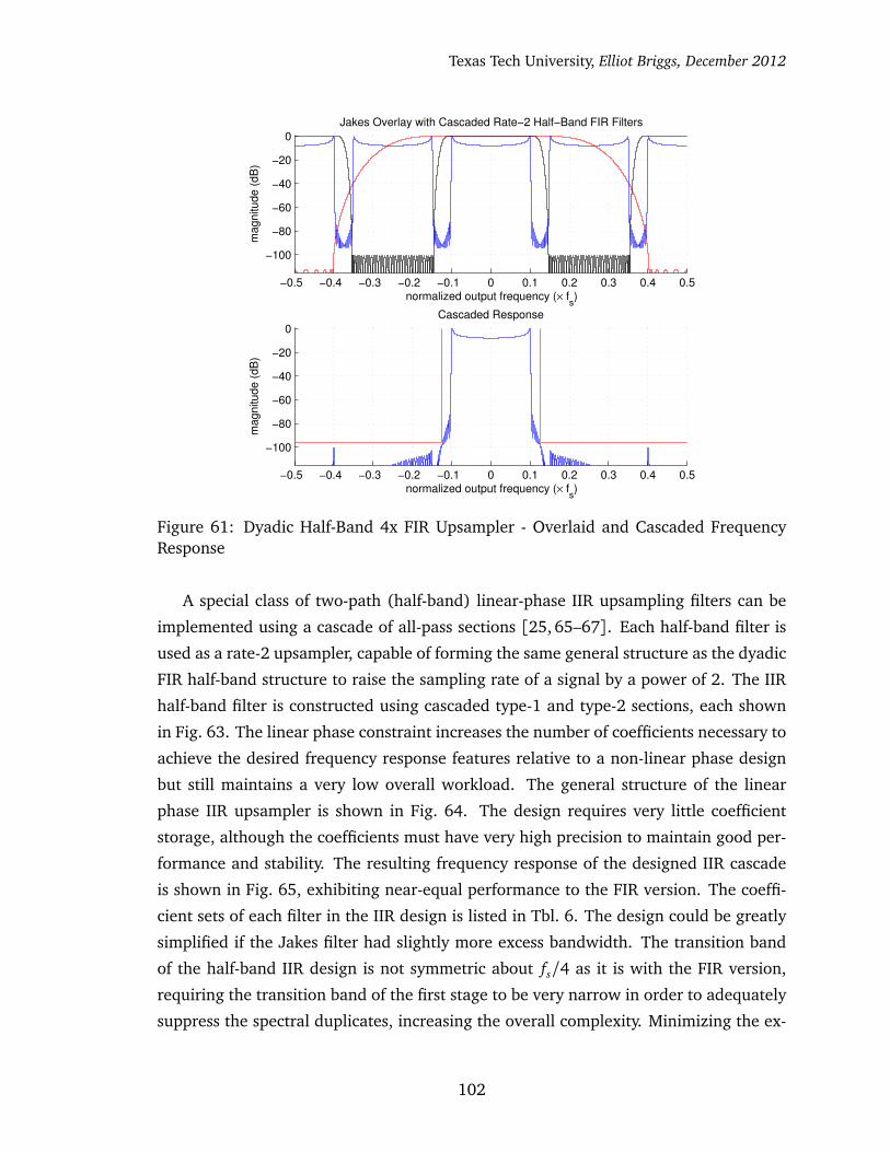
Texas Tech University, Elliot Briggs, December 2012
−0.5 −0.4 −0.3 −0.2 −0.1 0 0.1 0.2 0.3 0.4 0.5
−100
−80
−60
−40
−20
0
Cascaded Response
ma
gn
itu
de
(d
B)
normalized output frequency (× fs)
−0.5 −0.4 −0.3 −0.2 −0.1 0 0.1 0.2 0.3 0.4 0.5
−100
−80
−60
−40
−20
0
Jakes Overlay with Cascaded Rate−2 Half−Band FIR Filters
ma
gn
itu
de
(d
B)
normalized output frequency (× fs)
Figure 61: Dyadic Half-Band 4x FIR Upsampler - Overlaid and Cascaded FrequencyResponse
A special class of two-path (half-band) linear-phase IIR upsampling filters can be
implemented using a cascade of all-pass sections [25, 65–67]. Each half-band filter is
used as a rate-2 upsampler, capable of forming the same general structure as the dyadic
FIR half-band structure to raise the sampling rate of a signal by a power of 2. The IIR
half-band filter is constructed using cascaded type-1 and type-2 sections, each shown
in Fig. 63. The linear phase constraint increases the number of coefficients necessary to
achieve the desired frequency response features relative to a non-linear phase design
but still maintains a very low overall workload. The general structure of the linear
phase IIR upsampler is shown in Fig. 64. The design requires very little coefficient
storage, although the coefficients must have very high precision to maintain good per-
formance and stability. The resulting frequency response of the designed IIR cascade
is shown in Fig. 65, exhibiting near-equal performance to the FIR version. The coeffi-
cient sets of each filter in the IIR design is listed in Tbl. 6. The design could be greatly
simplified if the Jakes filter had slightly more excess bandwidth. The transition band
of the half-band IIR design is not symmetric about fs/4 as it is with the FIR version,
requiring the transition band of the first stage to be very narrow in order to adequately
suppress the spectral duplicates, increasing the overall complexity. Minimizing the ex-
102
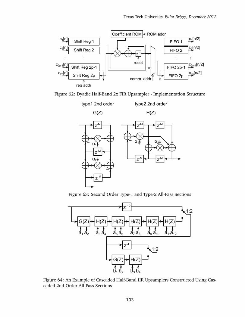
Texas Tech University, Elliot Briggs, December 2012
z-1
reset
Coefficient ROM
reg addr
comm. addr
ROM addr
...FIFO 2p-1
FIFO 2p
FIFO 1
Shift Reg 2
...
Shift Reg 2p-1
Shift Reg 2p
Shift Reg 1
FIFO 2
... ...
c1[n/2]
c2[n/2]
c2p-1[n/2]
c2p[n/2]
c1[n]
c2[n]
c2p-1[n]
c2p[n]
Figure 62: Dyadic Half-Band 2x FIR Upsampler - Implementation Structure
α1
z-M
z-M
_
_
α2
z-M
α1
z-M z-M
z-M
_α2
_
z-M
type1 2nd order type2 2nd order
G(Z) H(Z)
Figure 63: Second Order Type-1 and Type-2 All-Pass Sections
1:2
1:2z-4
G(Z) H(Z)
b1 b2 b3 b4
z-12
G(Z)
a1 a2
H(Z) H(Z)
a9 a10 a11a12
H(Z) H(Z)
a5 a6 a7 a8
H(Z)
a3 a4
Figure 64: An Example of Cascaded Half-Band IIR Upsamplers Constructed Using Cas-caded 2nd-Order All-Pass Sections
103
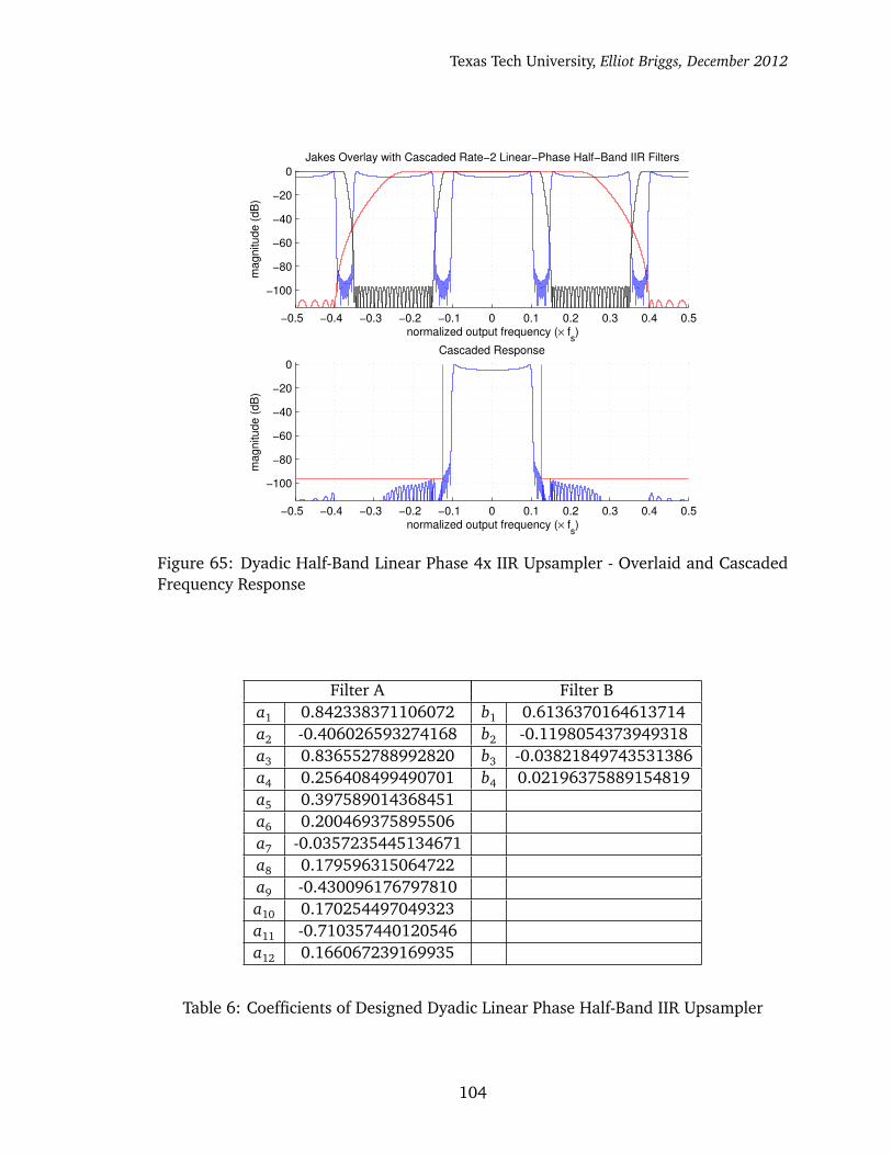
Texas Tech University, Elliot Briggs, December 2012
−0.5 −0.4 −0.3 −0.2 −0.1 0 0.1 0.2 0.3 0.4 0.5
−100
−80
−60
−40
−20
0
Jakes Overlay with Cascaded Rate−2 Linear−Phase Half−Band IIR Filters
ma
gn
itu
de
(d
B)
normalized output frequency (× fs)
−0.5 −0.4 −0.3 −0.2 −0.1 0 0.1 0.2 0.3 0.4 0.5
−100
−80
−60
−40
−20
0
Cascaded Response
ma
gn
itu
de
(d
B)
normalized output frequency (× fs)
Figure 65: Dyadic Half-Band Linear Phase 4x IIR Upsampler - Overlaid and CascadedFrequency Response
Filter A Filter Ba1 0.842338371106072 b1 0.6136370164613714a2 -0.406026593274168 b2 -0.1198054373949318a3 0.836552788992820 b3 -0.03821849743531386a4 0.256408499490701 b4 0.02196375889154819a5 0.397589014368451a6 0.200469375895506a7 -0.0357235445134671a8 0.179596315064722a9 -0.430096176797810a10 0.170254497049323a11 -0.710357440120546a12 0.166067239169935
Table 6: Coefficients of Designed Dyadic Linear Phase Half-Band IIR Upsampler
104
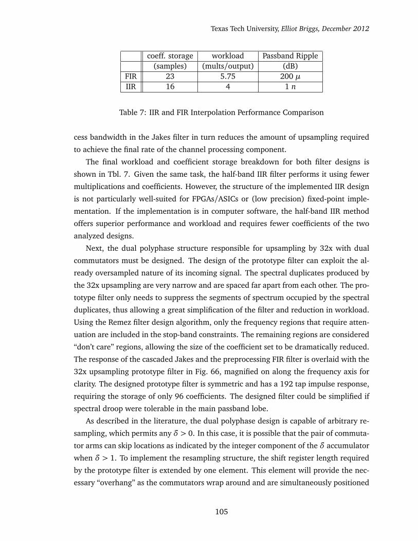
Texas Tech University, Elliot Briggs, December 2012
coeff. storage workload Passband Ripple(samples) (mults/output) (dB)
FIR 23 5.75 200 µIIR 16 4 1 n
Table 7: IIR and FIR Interpolation Performance Comparison
cess bandwidth in the Jakes filter in turn reduces the amount of upsampling required
to achieve the final rate of the channel processing component.
The final workload and coefficient storage breakdown for both filter designs is
shown in Tbl. 7. Given the same task, the half-band IIR filter performs it using fewer
multiplications and coefficients. However, the structure of the implemented IIR design
is not particularly well-suited for FPGAs/ASICs or (low precision) fixed-point imple-
mentation. If the implementation is in computer software, the half-band IIR method
offers superior performance and workload and requires fewer coefficients of the two
analyzed designs.
Next, the dual polyphase structure responsible for upsampling by 32x with dual
commutators must be designed. The design of the prototype filter can exploit the al-
ready oversampled nature of its incoming signal. The spectral duplicates produced by
the 32x upsampling are very narrow and are spaced far apart from each other. The pro-
totype filter only needs to suppress the segments of spectrum occupied by the spectral
duplicates, thus allowing a great simplification of the filter and reduction in workload.
Using the Remez filter design algorithm, only the frequency regions that require atten-
uation are included in the stop-band constraints. The remaining regions are considered
“don’t care” regions, allowing the size of the coefficient set to be dramatically reduced.
The response of the cascaded Jakes and the preprocessing FIR filter is overlaid with the
32x upsampling prototype filter in Fig. 66, magnified on along the frequency axis for
clarity. The designed prototype filter is symmetric and has a 192 tap impulse response,
requiring the storage of only 96 coefficients. The designed filter could be simplified if
spectral droop were tolerable in the main passband lobe.
As described in the literature, the dual polyphase design is capable of arbitrary re-
sampling, which permits any δ > 0. In this case, it is possible that the pair of commuta-
tor arms can skip locations as indicated by the integer component of the δ accumulator
when δ > 1. To implement the resampling structure, the shift register length required
by the prototype filter is extended by one element. This element will provide the nec-
essary “overhang” as the commutators wrap around and are simultaneously positioned
105
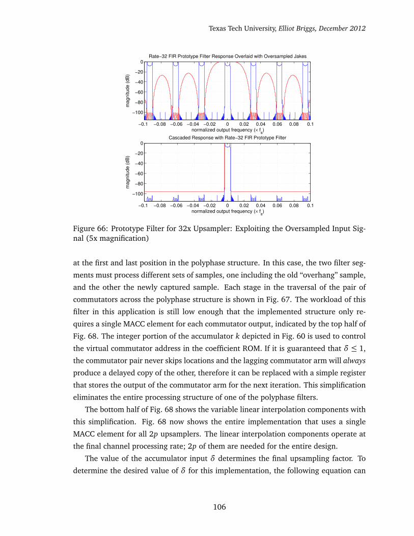
Texas Tech University, Elliot Briggs, December 2012
−0.1 −0.08 −0.06 −0.04 −0.02 0 0.02 0.04 0.06 0.08 0.1
−100
−80
−60
−40
−20
0Rate−32 FIR Prototype Filter Response Overlaid with Oversampled Jakes
ma
gn
itu
de
(d
B)
normalized output frequency (× fs)
−0.1 −0.08 −0.06 −0.04 −0.02 0 0.02 0.04 0.06 0.08 0.1
−100
−80
−60
−40
−20
0Cascaded Response with Rate−32 FIR Prototype Filter
ma
gn
itu
de
(d
B)
normalized output frequency (× fs)
Figure 66: Prototype Filter for 32x Upsampler: Exploiting the Oversampled Input Sig-nal (5x magnification)
at the first and last position in the polyphase structure. In this case, the two filter seg-
ments must process different sets of samples, one including the old “overhang” sample,
and the other the newly captured sample. Each stage in the traversal of the pair of
commutators across the polyphase structure is shown in Fig. 67. The workload of this
filter in this application is still low enough that the implemented structure only re-
quires a single MACC element for each commutator output, indicated by the top half of
Fig. 68. The integer portion of the accumulator k depicted in Fig. 60 is used to control
the virtual commutator address in the coefficient ROM. If it is guaranteed that δ ≤ 1,
the commutator pair never skips locations and the lagging commutator arm will always
produce a delayed copy of the other, therefore it can be replaced with a simple register
that stores the output of the commutator arm for the next iteration. This simplification
eliminates the entire processing structure of one of the polyphase filters.
The bottom half of Fig. 68 shows the variable linear interpolation components with
this simplification. Fig. 68 now shows the entire implementation that uses a single
MACC element for all 2p upsamplers. The linear interpolation components operate at
the final channel processing rate; 2p of them are needed for the entire design.
The value of the accumulator input δ determines the final upsampling factor. To
determine the desired value of δ for this implementation, the following equation can
106
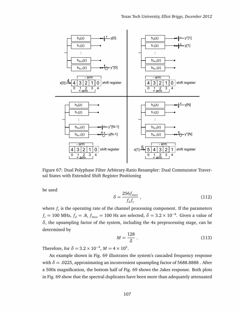
Texas Tech University, Elliot Briggs, December 2012
0 1 432
shift register 4 3 2 1 04
...
h0(z)
h1(z)
hN-2(z)
hN-1(z)_
+ y[0]
y*[0]
x[0]
- arm
+ arm
0 1 432
shift register 5 4 3 2 15
...
h0(z)
h1(z)
hN-2(z)
hN-1(z)_
+ y[N]
y*[N]
x[1]
- arm
+ arm
0 1 432
shift register 4 3 2 1 0...
h0(z)
h1(z)
hN-2(z)
hN-1(z)
+ y[1]
- arm
+ arm
_y*[1]
0 1 432
shift register 4 3 2 1 0
...
h0(z)
h1(z)
hN-2(z)
hN-1(z) + y[N-1]
- arm
+ arm
_y*[N-1]
Figure 67: Dual Polyphase Filter Arbitrary-Ratio Resampler: Dual Commutator Traver-sal States with Extended Shift Register Positioning
be used
δ =256 fmax
fd fs, (112)
where fs is the operating rate of the channel processing component. If the parameters
fs = 100 MHz, fd = .8, fmax = 100 Hz are selected, δ = 3.2× 10⁻⁴. Given a value of
δ, the upsampling factor of the system, including the 4x preprocessing stage, can be
determined by
M =128
δ. (113)
Therefore, for δ = 3.2× 10⁻⁴, M = 4× 10⁵.
An example shown in Fig. 69 illustrates the system’s cascaded frequency response
with δ = .0225, approximating an inconvenient upsampling factor of 5688.8888 . After
a 500x magnification, the bottom half of Fig. 69 shows the Jakes response. Both plots
in Fig. 69 show that the spectral duplicates have been more than adequately attenuated
107
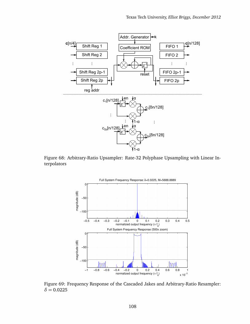
Texas Tech University, Elliot Briggs, December 2012
Coefficient ROM
reg addr
k
c[n/4]
Shift Reg 2
...
Shift Reg 2p-1
Shift Reg 2p
Shift Reg 1
... ...FIFO 2p-1
FIFO 2p
FIFO 1
FIFO 2
...
c[n/128]
z-1
reset
Addr. Generator
c1[n/128]z-1
α
1-α
c1[δn/128]
c2p[n/128]z-1
α
1-α
c2p[δn/128]
en
en
...
...
...
Figure 68: Arbitrary-Ratio Upsampler: Rate-32 Polyphase Upsampling with Linear In-terpolators
−0.5 −0.4 −0.3 −0.2 −0.1 0 0.1 0.2 0.3 0.4 0.5
−100
−50
0
normalized output frequency (× fs)
ma
gn
itu
de
(d
B)
Full System Frequency Response: δ=0.0225, M=5688.8889
−1 −0.8 −0.6 −0.4 −0.2 0 0.2 0.4 0.6 0.8 1
x 10−3
−100
−50
0
normalized output frequency (× fs)
ma
gn
itu
de
(d
B)
Full System Frequency Response (500x zoom)
Figure 69: Frequency Response of the Cascaded Jakes and Arbitrary-Ratio Resampler:δ = 0.0225
108
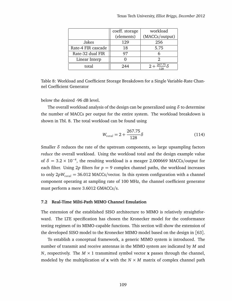
Texas Tech University, Elliot Briggs, December 2012
coeff. storage workload(elements) (MACCs/output)
Jakes 129 256Rate-4 FIR cascade 18 5.75Rate-32 dual FIR 97 6
Linear Interp 0 2
total 244 2+ 267.75128
δ
Table 8: Workload and Coefficient Storage Breakdown for a Single Variable-Rate Chan-nel Coefficient Generator
below the desired -96 dB level.
The overall workload analysis of the design can be generalized using δ to determine
the number of MACCs per output for the entire system. The workload breakdown is
shown in Tbl. 8. The total workload can be found using
Wtotal = 2+267.75
128δ (114)
Smaller δ reduces the rate of the upstream components, so large upsampling factors
reduce the overall workload. Using the workload total and the design example value
of δ = 3.2 × 10⁻⁴, the resulting workload is a meager 2.000669 MACCs/output for
each filter. Using 2p filters for p = 9 complex channel paths, the workload increases
to only 2pWtotal = 36.012 MACCs/vector. In this system configuration with a channel
component operating at sampling rate of 100 MHz, the channel coefficient generator
must perform a mere 3.6012 GMACCs/s.
7.2 Real-Time Milti-Path MIMO Channel Emulation
The extension of the established SISO architecture to MIMO is relatively straightfor-
ward. The LTE specification has chosen the Kronecker model for the conformance
testing regimen of its MIMO-capable functions. This section will show the extension of
the developed SISO model to the Kronecker MIMO model based on the design in [63].
To establish a conceptual framework, a generic MIMO system is introduced. The
number of transmit and receive antennas in the MIMO system are indicated by M and
N , respectively. The M × 1 transmitted symbol vector x passes through the channel,
modeled by the multiplication of x with the N × M matrix of complex channel path
109

Texas Tech University, Elliot Briggs, December 2012
x[t]Δt2
H1[t]
Δt3
H2[t]
Δtp...
Hp[t]...
...
Σ
y[t]
Figure 70: Tapped Delay Line MIMO Channel Model
coefficients H, the channel matrix, to form the received N × 1 symbol vector y.
y= Hx
y1
y2...
yN
=
h1,1 h1,2 · · · h1,M
h2,1 h2,2 · · · h2,M...
.... . .
...
hN ,1 hN ,2 · · · hN ,M
x1
x2...
xM
(115)
The multiplication between H and x models the passage of the N transmitted symbols
traveling through N M paths in the channel, which are then summed accordingly at the
receiver’s N antennas. To add the capability of the model to describe channels with
mobility, time indices are added to each element in Eq. 115, consequently adding time
indices to the individual elements that comprise both vectors and the channel matrix.
y [t] = H [t]x [t] (116)
For the multi-path case, the channel can be modeled by
A (t,τ) =P∑
i=1
Hi [t]δ�
τ−τi�
. (117)
and pictorially described by the structure shown in Fig. 70. Each channel path now has
its own matrix of complex weights. To keep the model simple, it has been assumed that
the paths that make the elements in each channel matrix have the same p× 1 delay
vector τ =�
τ1 = 0,τ2, . . . ,τp
�T, where each element is a positive continuous-time
delay.
The capacity of the SISO channel, i.e. M = N = 1 is given by [68]
C = log2
�
1+ρh2�
b/s/Hz (118)
110

Texas Tech University, Elliot Briggs, December 2012
where h is the normalized complex gain of the stationary, or the instantaneous real-
ization of a mobile channel, and ρ is the SNR at the receiver. In a MIMO system, the
channel’s capacity is defined by
CEP = log2
�
det�
IM +ρ
NHHH
��
b/s/Hz (119)
assuming equal power (EP) uncorrelated sources [68, 69]. The channel’s capacity
grows linearly with min (M , N). The determinant operator yields a product of min (M , N)
non-zero eigenvalues, which are determined by the properties of the channel matrix.
Each eigenvalue characterizes the SNR over the channel “eigenmode”. The channel’s
capacity is determined by the sum of the capacities of each individual eigenmode,
therefore the capacity increases with additional antennas and the spatial properties of
the channel [68]. Intuitively, an orthonormal channel matrix maximizes the channel’s
capacity.
In a mobile channel, the elements of the H matrix become time-varying, and HHH
in Eq. 119 is replaced with E�
HHH�, which determines the expected channel capac-
ity determined by the statistics of the channel matrix. Clearly, the statistics of the
time-varying behavior of the channel matrix have a profound impact on the emulated
system.
In the special case where each element in H is i.i.d., each “sub-channel” is spatially
independent, or uncorrelated, maximizing capacity by diagonalizing the expected value
of the HHH term and maximizing the value produced by the determinant in Eq. 119.
The i.i.d. assumption can still hold using Jakes processes in each subchannel [70],
which models the Doppler spectrum and temporal correlation properties of a typical
channel scenario with mobility. Each Jakes processes can be generated in real-time
using the Jakes process generator developed in Sec. 7.1.
In a realistic mobile scenario, the antennas on the mobile device are confined to a
small area, restricting the spacing between each antenna and limiting the achievable
spatial diversity. The base station antenna array is less restricted for space and can offer
better spatial diversity. The spatial characteristics of the channel and the properties of
the two antenna arrays introduce spatial correlation, revoking the ideal i.i.d. aspect of
the elements in H. With the i.i.d. assumption removed, the expected value of the HHH
term begins growing off-diagonal elements, decreasing the eigenvalues and decreasing
the channel’s capacity from its maximum.
Establishing an accurate model for some common antenna configurations and chan-
nel conditions allows the spatial correlation properties to be user-selectable, just as the
111
Texas Tech University, Elliot Briggs, December 2012
Jakes model allows the user to select the temporal correlation by providing the velocity
of the mobile device and the carrier frequency. One popular model that allows this is
the Kronecker model, first introduced and verified in [70–72]. However, this model has
been claimed to be too “simplistic” and can be invalid for some special cases [73, 74].
The method presented in [74] adds a small modification to the Kronecker model that
significantly increases the accuracy of the modeled channel capacity in the many illus-
trated cases where the Kronecker model fails.
Despite the claimed inaccuracies, presently, the Kronecker model is very relevant;
the simple model is used in the LTE standard [42] among others for conformance
testing, making it desirable in the test equipment marketplace. Here, the Kronecker
model will be introduced along with its architecture as implemented and tested in
FPGA hardware in real-time.
The Kronecker model formulation starts by lumping the correlation properties of
the two antenna arrays and their local spatial features into correlation matrices. These
matrices represent the spatial statistics that result from antenna spacing, radiation pat-
tern, and the local scattering environment. According to [74], the two correlation
matrices accurately model the effects of the channel scatterers clustered around the
link ends, or antenna arrays, without considering any scatterers in between. This is an
accurate model for some cases in a cellular system. The base station antennas are typi-
cally surrounded by clutter from its antenna mast, while the mobile device is frequently
located in a clutter-filled environment such as a building or a vehicle. In this scenario,
assuming the base station and the mobile device are separated by a sparse scattering
environment such as free space, the assumptions made by the Kronecker model seem
conceivably valid.
To conceptualize the fundamental theory of the modeling as desribed by [68], the
power azimuth distribution function p (θ) is introduced, which defines the distribution
of scatterers in azimuth angle θ as seen by the base station, where θ ∈ [Θ−∆,Θ+∆],
Θ and ∆ indicating the angle of arrival at the receiver and the angle spread, respec-
tively. The angle spread is affected by the relative height between the base station and
the mobile device. The base station antennas are usually elevated above the mobile
device on an antenna mast. The angle of arrival is the angle at which the transmitted
signal energy arrives w.r.t. broadside at the receive antenna array. Given p (θ) and
using the notation in [68], the spacial correlation between the paths from receive and
112

Texas Tech University, Elliot Briggs, December 2012
transmit antennas Rn and Tm and Rn and Tm′ can be found using
Ψ�
RnTm, RnTm′�
=
∫ Θ+∆
Θ−∆p (θ)exp
�
j2πsin (θ)λ
D�
Tm, Tm′�
�
dθ , (120)
where D�
Tm, Tm′�
indicates the distance between antennas Tm and Tm′ , and n ∈ [1,2 . . . , N],
and m ∈ [1,2 . . . , M], and the prime simply indicates n 6= n′ and m 6= m′. The Kro-
necker model approximates the correlation matrix Ψ by performing the Kronecker
product between the local transmit and receive correlation matrices ΨT X and ΨRX .
Ψ≈ΨRX ⊗ΨT X (121)
The statements regarding the Kronecker model inaccuracies in [74] are now more in-
tuitive with the added context. The model only considers the spatial channel features
immediately surrounding each antenna array that make up the correlation matrices, in-
dependently of the other, and independently of the channel features that exist between
the two arrays.
To apply the desired spatial correlation properties to the matrix of i.i.d. channel
coefficient processes, the Ψ matrix is first decomposed using Cholesky decomposition,
resulting in the product of the all-real lower-diagonal C matrix and its transpose.
Ψ= CCT (122)
The C matrix is then multiplied by j, the vectorized matrix of i.i.d. complex Jakes
113
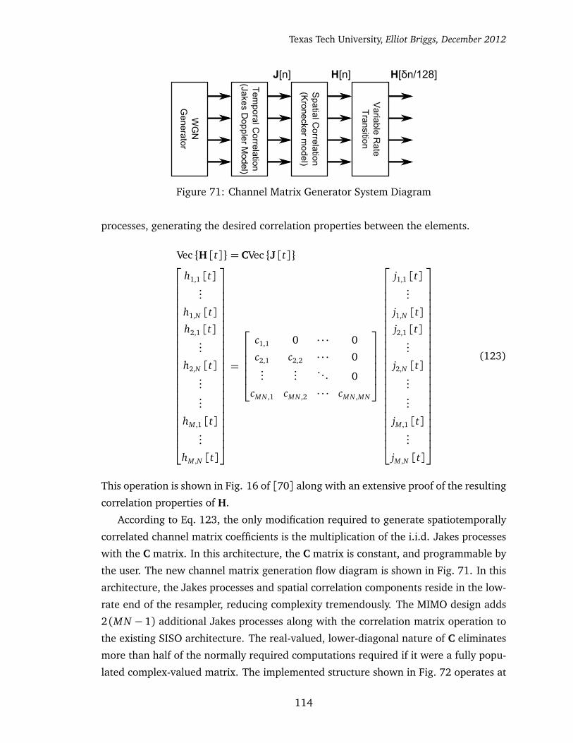
Texas Tech University, Elliot Briggs, December 2012
Spatial C
orrelation(K
ronecker model)
Tem
poral Correlation
(Jakes Doppler M
odel)
Variable R
ateT
ransition
WG
NG
enerator
J[n] H[n] H[δn/128]
Figure 71: Channel Matrix Generator System Diagram
processes, generating the desired correlation properties between the elements.
Vec {H [t]}= CVec {J [t]}
h1,1 [t]...
h1,N [t]
h2,1 [t]...
h2,N [t]......
hM ,1 [t]...
hM ,N [t]
=
c1,1 0 · · · 0
c2,1 c2,2 · · · 0...
.... . . 0
cMN ,1 cMN ,2 · · · cMN ,MN
j1,1 [t]...
j1,N [t]
j2,1 [t]...
j2,N [t]......
jM ,1 [t]...
jM ,N [t]
(123)
This operation is shown in Fig. 16 of [70] along with an extensive proof of the resulting
correlation properties of H.
According to Eq. 123, the only modification required to generate spatiotemporally
correlated channel matrix coefficients is the multiplication of the i.i.d. Jakes processes
with the C matrix. In this architecture, the C matrix is constant, and programmable by
the user. The new channel matrix generation flow diagram is shown in Fig. 71. In this
architecture, the Jakes processes and spatial correlation components reside in the low-
rate end of the resampler, reducing complexity tremendously. The MIMO design adds
2 (MN − 1) additional Jakes processes along with the correlation matrix operation to
the existing SISO architecture. The real-valued, lower-diagonal nature of C eliminates
more than half of the normally required computations required if it were a fully popu-
lated complex-valued matrix. The implemented structure shown in Fig. 72 operates at
114
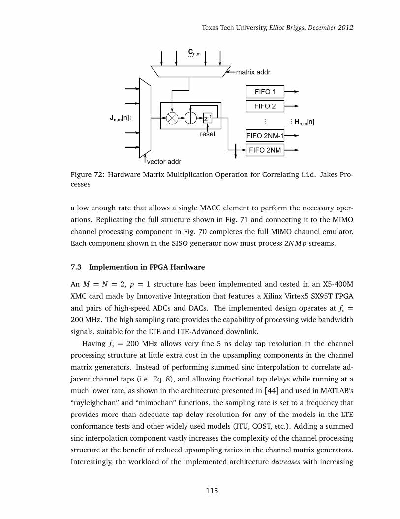
Texas Tech University, Elliot Briggs, December 2012
Jn,m[n] ...
FIFO 1
FIFO 2
FIFO 2NM-1
FIFO 2NM
Hn,m[n]z-1
reset
...
Cn,m...
matrix addr
vector addr
...
Figure 72: Hardware Matrix Multiplication Operation for Correlating i.i.d. Jakes Pro-cesses
a low enough rate that allows a single MACC element to perform the necessary oper-
ations. Replicating the full structure shown in Fig. 71 and connecting it to the MIMO
channel processing component in Fig. 70 completes the full MIMO channel emulator.
Each component shown in the SISO generator now must process 2N M p streams.
7.3 Implemention in FPGA Hardware
An M = N = 2, p = 1 structure has been implemented and tested in an X5-400M
XMC card made by Innovative Integration that features a Xilinx Virtex5 SX95T FPGA
and pairs of high-speed ADCs and DACs. The implemented design operates at fs =
200 MHz. The high sampling rate provides the capability of processing wide bandwidth
signals, suitable for the LTE and LTE-Advanced downlink.
Having fs = 200 MHz allows very fine 5 ns delay tap resolution in the channel
processing structure at little extra cost in the upsampling components in the channel
matrix generators. Instead of performing summed sinc interpolation to correlate ad-
jacent channel taps (i.e. Eq. 8), and allowing fractional tap delays while running at a
much lower rate, as shown in the architecture presented in [44] and used in MATLAB’s
“rayleighchan” and “mimochan” functions, the sampling rate is set to a frequency that
provides more than adequate tap delay resolution for any of the models in the LTE
conformance tests and other widely used models (ITU, COST, etc.). Adding a summed
sinc interpolation component vastly increases the complexity of the channel processing
structure at the benefit of reduced upsampling ratios in the channel matrix generators.
Interestingly, the workload of the implemented architecture decreases with increasing
115
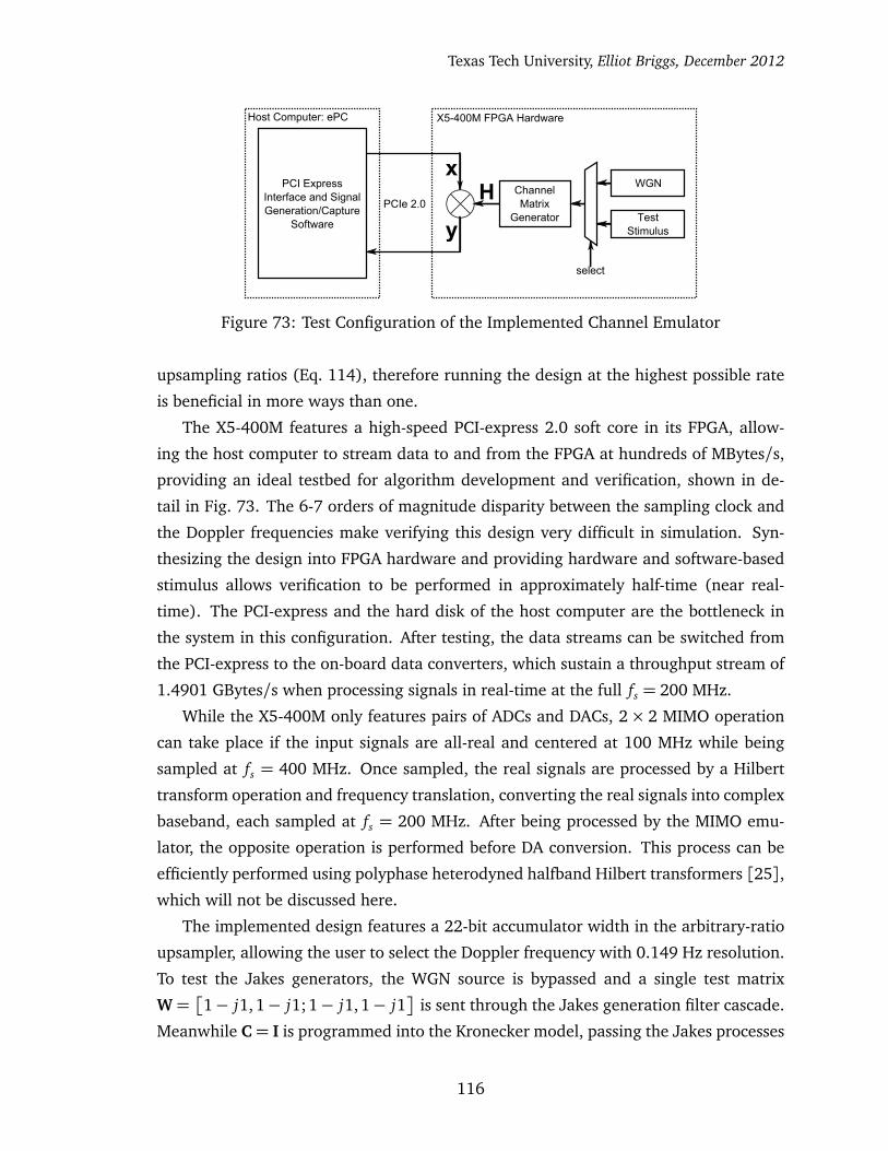
Texas Tech University, Elliot Briggs, December 2012
PCI ExpressInterface and SignalGeneration/Capture
Software
Host Computer: ePC
PCIe 2.0
X5-400M FPGA Hardware
ChannelMatrix
Generator TestStimulus
WGNH
x
y
select
Figure 73: Test Configuration of the Implemented Channel Emulator
upsampling ratios (Eq. 114), therefore running the design at the highest possible rate
is beneficial in more ways than one.
The X5-400M features a high-speed PCI-express 2.0 soft core in its FPGA, allow-
ing the host computer to stream data to and from the FPGA at hundreds of MBytes/s,
providing an ideal testbed for algorithm development and verification, shown in de-
tail in Fig. 73. The 6-7 orders of magnitude disparity between the sampling clock and
the Doppler frequencies make verifying this design very difficult in simulation. Syn-
thesizing the design into FPGA hardware and providing hardware and software-based
stimulus allows verification to be performed in approximately half-time (near real-
time). The PCI-express and the hard disk of the host computer are the bottleneck in
the system in this configuration. After testing, the data streams can be switched from
the PCI-express to the on-board data converters, which sustain a throughput stream of
1.4901 GBytes/s when processing signals in real-time at the full fs = 200 MHz.
While the X5-400M only features pairs of ADCs and DACs, 2× 2 MIMO operation
can take place if the input signals are all-real and centered at 100 MHz while being
sampled at fs = 400 MHz. Once sampled, the real signals are processed by a Hilbert
transform operation and frequency translation, converting the real signals into complex
baseband, each sampled at fs = 200 MHz. After being processed by the MIMO emu-
lator, the opposite operation is performed before DA conversion. This process can be
efficiently performed using polyphase heterodyned halfband Hilbert transformers [25],
which will not be discussed here.
The implemented design features a 22-bit accumulator width in the arbitrary-ratio
upsampler, allowing the user to select the Doppler frequency with 0.149 Hz resolution.
To test the Jakes generators, the WGN source is bypassed and a single test matrix
W=�
1− j1, 1− j1;1− j1, 1− j1�
is sent through the Jakes generation filter cascade.
Meanwhile C= I is programmed into the Kronecker model, passing the Jakes processes
116
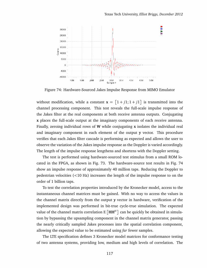
Texas Tech University, Elliot Briggs, December 2012
Figure 74: Hardware-Sourced Jakes Impulse Response from MIMO Emulator
without modification, while a constant x =�
1+ j1; 1+ j1�
is transmitted into the
channel processing component. This test reveals the full-scale impulse response of
the Jakes filter at the real components at both receive antenna outputs. Conjugating
x places the full-scale output at the imaginary components of each receive antenna.
Finally, zeroing individual rows of W while conjugating x isolates the individual real
and imaginary component in each element of the output y vector. This procedure
verifies that each Jakes filter cascade is performing as expected and allows the user to
observe the variation of the Jakes impulse response as the Doppler is varied accordingly.
The length of the impulse response lengthens and shortens with the Doppler setting.
The test is performed using hardware-sourced test stimulus from a small ROM lo-
cated in the FPGA, as shown in Fig. 73. The hardware-source test results in Fig. 74
show an impulse response of approximately 40 million taps. Reducing the Doppler to
pedestrian velocities (<10 Hz) increases the length of the impulse response to on the
order of 1 billion taps.
To test the correlation properties introduced by the Kronecker model, access to the
instantaneous channel matrices must be gained. With no way to access the values in
the channel matrix directly from the output y vector in hardware, verification of the
implemented design was performed in bit-true cycle-true simulation. The expected
value of the channel matrix correlation E�
HHH� can be quickly be obtained in simula-
tion by bypassing the upsampling component in the channel matrix generator, passing
the nearly critically sampled Jakes processes into the spatial correlation component,
allowing the expected value to be estimated using far fewer samples.
The LTE specification defines 3 Kronecker model matrices for conformance testing
of two antenna systems, providing low, medium and high levels of correlation. The
117

Texas Tech University, Elliot Briggs, December 2012
Used Available Percentageslices 1,646 14,720 11%BRAM 6 244 2%DSP48E 38 640 6%
Table 9: FPGA Resource Consumption for a Single Channel Matrix Generator, ExcludingWGN Source ( fs = 200 MHz)
simulation results along with both correlation matrices taken from the LTE specification
for each antenna array are shown below. RHH is the result obtained after averaging
500,000 HHH operations, closely estimating E�
HHH�.
ΨT Xlow =Ψ
RXlow =
1 0
0 1
RHH =
0.9994 0.0003+ j0.0009
0.0003− j0.0009 0.9994
(124)
ΨT Xmed =
1 .3
.3 1
,ΨRXmed =
1 .9
.9 1
RHH =
1.0001 0.2996− j0.0004
0.2996+ j0.0004 0.9982
(125)
ΨT Xhigh =Ψ
RXhigh =
1 .9
.9 1
RHH =
1.0001 0.9003+ j0.0003
0.9003− j0.0003 1.0002
(126)
The correlation results show good correspondence with the correlation matrices pro-
vided by the model. The matrices defined in the medium correlation scenario in Eq. 125
reinforce the earlier assumptions about the impact of antenna spacing and spatial cor-
relation at the base station and the mobile device.
The final resource consumption tabulation in Tbl. 9 reveals a very hardware ef-
ficient implementation, occupying a small fraction of the resources available in the
Virtex5 SX95T FPGA. The implemented model contains a single coefficient matrix gen-
erator, which leaves the components before the variable rate transition idle much of
the time. Increasing the number of channel paths keeps these components busier. The
expected hardware resource consumption should not dramatically increase with M and
118
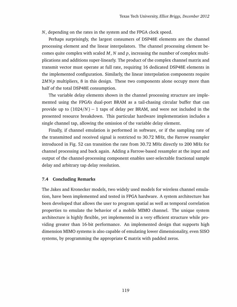
Texas Tech University, Elliot Briggs, December 2012
N , depending on the rates in the system and the FPGA clock speed.
Perhaps surprisingly, the largest consumers of DSP48E elements are the channel
processing element and the linear interpolators. The channel processing element be-
comes quite complex with scaled M , N and p, increasing the number of complex multi-
plications and additions super-linearly. The product of the complex channel matrix and
transmit vector must operate at full rate, requiring 16 dedicated DSP48E elements in
the implemented configuration. Similarly, the linear interpolation components require
2MN p multipliers, 8 in this design. These two components alone occupy more than
half of the total DSP48E consumption.
The variable delay elements shown in the channel processing structure are imple-
mented using the FPGA’s dual-port BRAM as a tail-chasing circular buffer that can
provide up to (1024/N) − 1 taps of delay per BRAM, and were not included in the
presented resource breakdown. This particular hardware implementation includes a
single channel tap, allowing the omission of the variable delay element.
Finally, if channel emulation is performed in software, or if the sampling rate of
the transmitted and received signal is restricted to 30.72 MHz, the Farrow resampler
introduced in Fig. 52 can transition the rate from 30.72 MHz directly to 200 MHz for
channel processing and back again. Adding a Farrow-based resampler at the input and
output of the channel-processing component enables user-selectable fractional sample
delay and arbitrary tap delay resolution.
7.4 Concluding Remarks
The Jakes and Kronecker models, two widely used models for wireless channel emula-
tion, have been implemented and tested in FPGA hardware. A system architecture has
been developed that allows the user to program spatial as well as temporal correlation
properties to emulate the behavior of a mobile MIMO channel. The unique system
architecture is highly flexible, yet implemented in a very efficient structure while pro-
viding greater than 16-bit performance. An implemented design that supports high
dimension MIMO systems is also capable of emulating lower dimensionality, even SISO
systems, by programming the appropriate C matrix with padded zeros.
119

Texas Tech University, Elliot Briggs, December 2012
8 Conclusions
This dissertation has covered a wide range of topics with several notable contributions.
Ch. 3 introduces OFDM receiver synchronization concepts, showing a connection be-
tween sampling frequency offset and symbol timing synchronization. A receiver ar-
chitecture was introduced that simultaneously corrects sampling frequency offset and
symbol timing. The technique was shown to maintain excellent performance, even in
harsh multi-path highly-mobile channel conditions. To enhance performance in an LTE
system, a technique was developed that is able to efficiently detect symbol timing using
the primary synchronization signal (PSS) in the time domain. The detection method
exploits the band-limited nature of the PSS to minimize the number of necessary com-
putations.
Ch. 4 continued with the LTE OFDM receiver design by first introducing a stochastic
optimization technique to directly estimate the equalization matrix using the received
signal and the available reference symbols (RSs). Exploration of an alternative method
was introduced using locally weighted regression. The regression technique features
a parametrized kernel that can be selected for a particular channel environment. The
kernel selection was found using offline training. The regression technique was shown
to significantly reduce estimation error in two out of the three LTE-specified channel
environments.
The regression technique used for channel estimation was found to be quite use-
ful for other tasks, such as arbitrary-ratio resampling. Ch. 5 showed that the locally
weighted regression algorithm can be formulated to generate the Farrow filter. Us-
ing a parametrized kernel, the response of the Farrow filter can be adjusted. Using a
pre-processing upsampler, the Farrow filter was found to exhibit excellent resampling
performance, which was demonstrated in the simulation results of Ch. 3.
Later, in Ch. 6 a technique that utilizes cyclic prefix redundancy was introduced,
capable of providing modest SNR improvements in an OFDM receiver operating in
“normal channel conditions”. The redundancy combination is performed using a single
addition and bit-shift for each received sample. The technique requires already-known
or readily available measurements of the channel’s excess delay.
Finally, Ch. 7 presents the theory and implementation of a real-time multi-path
MIMO fading channel emulator. The developed architecture was implemented and
tested in FPGA hardware. The unique architecture utilizes an arbitrary-ratio resampler
that guarantees 16-bit performance, enabling the user to select the desired Doppler
frequency at run-time with high resolution. The architecture also allows run-time pro-
120

Texas Tech University, Elliot Briggs, December 2012
graming of the spatial correlation aspects of the channel, which determines the ex-
pected channel capacity in a MIMO system. Hardware-based test results and FPGA
resource consumption reveal a very cost-effective, high-performance design.
121
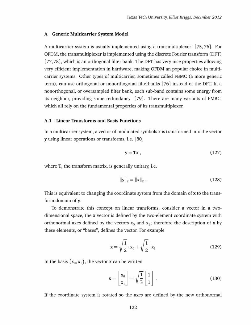
Texas Tech University, Elliot Briggs, December 2012
A Generic Multicarrier System Model
A multicarrier system is usually implemented using a transmultiplexer [75, 76]. For
OFDM, the transmultiplexer is implemented using the discrete Fourier transform (DFT)
[77,78], which is an orthogonal filter bank. The DFT has very nice properties allowing
very efficient implementation in hardware, making OFDM an popular choice in multi-
carrier systems. Other types of multicarrier, sometimes called FBMC (a more generic
term), can use orthogonal or nonorthogonal filterbanks [76] instead of the DFT. In a
nonorthogonal, or oversampled filter bank, each sub-band contains some energy from
its neighbor, providing some redundancy [79]. There are many variants of FMBC,
which all rely on the fundamental properties of its transmultiplexer.
A.1 Linear Transforms and Basis Functions
In a multicarrier system, a vector of modulated symbols x is transformed into the vector
y using linear operations or transforms, i.e. [80]
y= Tx , (127)
where T, the transform matrix, is generally unitary, i.e.
‖y‖2 = ‖x‖2 . (128)
This is equivalent to changing the coordinate system from the domain of x to the trans-
form domain of y.
To demonstrate this concept on linear transforms, consider a vector in a two-
dimensional space, the x vector is defined by the two-element coordinate system with
orthonormal axes defined by the vectors x0 and x1; therefore the description of x by
these elements, or “bases”, defines the vector. For example
x=
r
1
2· x0+
r
1
2· x1 (129)
In the basis�
x0, x1
�
, the vector x can be written
x=
x0
x1
=
r
1
2
1
1
. (130)
If the coordinate system is rotated so the axes are defined by the new orthonormal
122

Texas Tech University, Elliot Briggs, December 2012
x1
0-1 1
1
x0
x
Figure 75: Two-Element Vector Defined in the Orthonormal Basis�
x0, x1
�
x1
0-1 1
1
x0
yy0y1
Figure 76: Two-Element Vector Redefined in the Orthonormal Basis�
y0, y1
�
basis�
y0, y1
�
, the old x vector can still be expressed in the new transformed basis as
the vector y (Fig. 76). For this example, let
y= 1 · y0+ 0 · y1 (131)
Using the basis�
y0, y1
�
, the vector y can be written
y=
y0
y1
=
1
0
. (132)
The same vector can be expressed both in the x and y basis. The coordinate systems
can be related using the following expression using the vectors shown in Fig. 77.
y0
y1
=
yT0 x0 yT
0 x1
yT1 x0 yT
1 x1
x0
x1
=
r
1
2
1 1
−1 1
x0
x1
, (133)
123
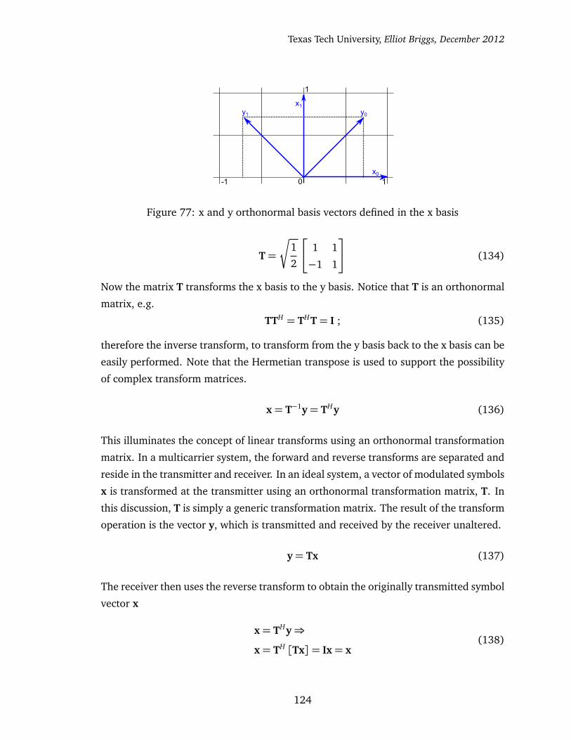
Texas Tech University, Elliot Briggs, December 2012
x1
0-1 1
1
x0
y0y1
Figure 77: x and y orthonormal basis vectors defined in the x basis
T=
r
1
2
1 1
−1 1
(134)
Now the matrix T transforms the x basis to the y basis. Notice that T is an orthonormal
matrix, e.g.
TTH = THT= I ; (135)
therefore the inverse transform, to transform from the y basis back to the x basis can be
easily performed. Note that the Hermetian transpose is used to support the possibility
of complex transform matrices.
x= T−1y= THy (136)
This illuminates the concept of linear transforms using an orthonormal transformation
matrix. In a multicarrier system, the forward and reverse transforms are separated and
reside in the transmitter and receiver. In an ideal system, a vector of modulated symbols
x is transformed at the transmitter using an orthonormal transformation matrix, T. In
this discussion, T is simply a generic transformation matrix. The result of the transform
operation is the vector y, which is transmitted and received by the receiver unaltered.
y= Tx (137)
The receiver then uses the reverse transform to obtain the originally transmitted symbol
vector x
x= THy⇒
x= TH [Tx] = Ix= x(138)
124
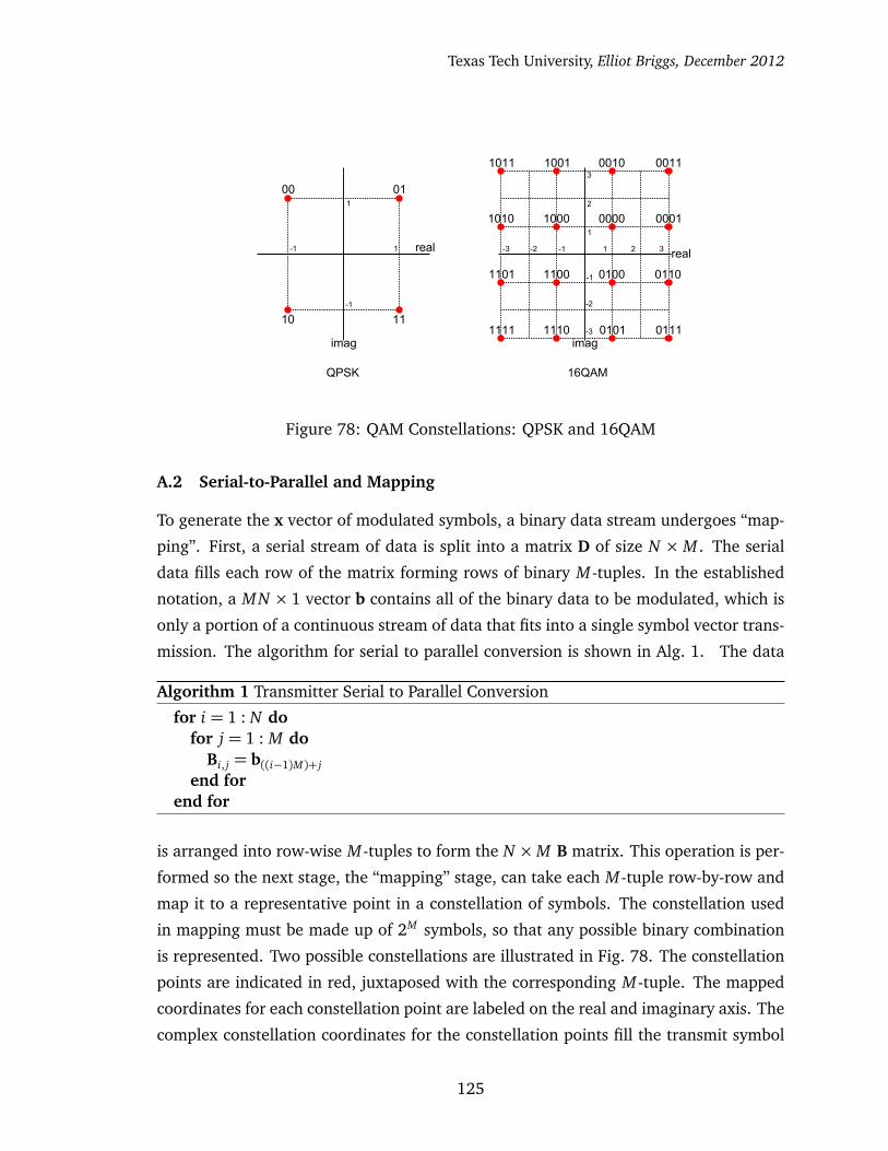
Texas Tech University, Elliot Briggs, December 2012
1
1
-1
-1 real
imag
00 01
10 11
real
imag
0000 000110001010
0100 011011001101
0101 011111101111
0010 001110011011
-1-2-3 1 2 3
1
2
3
-1
-2
-3
QPSK 16QAM
Figure 78: QAM Constellations: QPSK and 16QAM
A.2 Serial-to-Parallel and Mapping
To generate the x vector of modulated symbols, a binary data stream undergoes “map-
ping”. First, a serial stream of data is split into a matrix D of size N × M . The serial
data fills each row of the matrix forming rows of binary M -tuples. In the established
notation, a MN × 1 vector b contains all of the binary data to be modulated, which is
only a portion of a continuous stream of data that fits into a single symbol vector trans-
mission. The algorithm for serial to parallel conversion is shown in Alg. 1. The data
Algorithm 1 Transmitter Serial to Parallel Conversion
for i = 1 : N dofor j = 1 : M do
Bi, j = b((i−1)M)+ j
end forend for
is arranged into row-wise M -tuples to form the N ×M B matrix. This operation is per-
formed so the next stage, the “mapping” stage, can take each M -tuple row-by-row and
map it to a representative point in a constellation of symbols. The constellation used
in mapping must be made up of 2M symbols, so that any possible binary combination
is represented. Two possible constellations are illustrated in Fig. 78. The constellation
points are indicated in red, juxtaposed with the corresponding M -tuple. The mapped
coordinates for each constellation point are labeled on the real and imaginary axis. The
complex constellation coordinates for the constellation points fill the transmit symbol
125
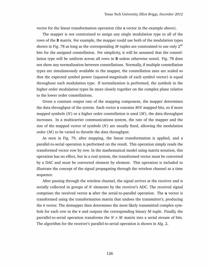
Texas Tech University, Elliot Briggs, December 2012
vector for the linear transformation operation (the x vector in the example above).
The mapper is not constrained to assign any single modulation type to all of the
rows of the B matrix. For example, the mapper could use both of the modulation types
shown in Fig. 78 as long as the corresponding M -tuples are constrained to use only 2M
bits for the assigned constellation. For simplicity, it will be assumed that the constel-
lation type will be uniform across all rows in B unless otherwise noted. Fig. 78 does
not show any normalization between constellations. Normally, if multiple constellation
types are simulaneously available to the mapper, the constellation axes are scaled so
that the expected symbol power (squared-magnitude of each symbol vector) is equal
throughout each modulation type. If normalization is performed, the symbols in the
higher order modulation types lie more closely together on the complex plane relative
to the lower order constellations.
Given a constant output rate of the mapping component, the mapper determines
the data throughput of the system. Each vector x contains MN mapped bits, so if more
mapped symbols (N) or a higher order constellation is used (M), the data throughput
increases. In a multicarrier communications system, the rate of the mapper and the
size of the mapped vector of symbols (N) are usually fixed, allowing the modulation
order (M) to be varied to throttle the data throughput.
As seen in Fig. 79, after mapping, the linear transformation is applied, and a
parallel-to-serial operation is performed on the result. This operation simply reads the
transformed vector row by row. In the mathematical model using matrix notation, this
operation has no effect, but in a real system, the transformed vector must be converted
by a DAC and must be converted element by element. This operation is included to
illustrate the concept of the signal propagating through the wireless channel as a time
sequence.
After passing through the wireless channel, the signal arrives at the receiver and is
serially collected in groups of N elements by the receiver’s ADC. The received signal
comprises the received vector u after the serial-to-parallel operation. The u vector is
transformed using the transformation matrix that undoes the transmitter’s, producing
the v vector. The demapper then determines the most likely transmitted complex sym-
bols for each row in the v and outputs the corresponding binary M -tuple. Finally, the
parrallel-to-serial operation transforms the N × M matrix into a serial stream of bits.
The algorithm for the receiver’s parallel-to-serial operation is shown in Alg. 2.
126
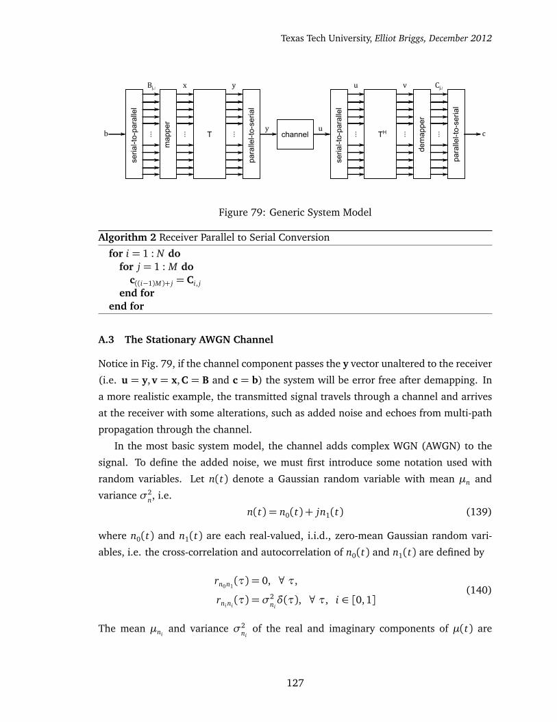
Texas Tech University, Elliot Briggs, December 2012
mapper
serial-to-parallel
...
Bj,:
b
... T
x
parallel-to-serial
... channel
serial-to-parallel
y
y u ...
u
TH
demapper
... ...
parallel-to-serial
c
Cj,:v
Figure 79: Generic System Model
Algorithm 2 Receiver Parallel to Serial Conversion
for i = 1 : N dofor j = 1 : M do
c((i−1)M)+ j = Ci, j
end forend for
A.3 The Stationary AWGN Channel
Notice in Fig. 79, if the channel component passes the y vector unaltered to the receiver
(i.e. u = y,v = x,C = B and c = b) the system will be error free after demapping. In
a more realistic example, the transmitted signal travels through a channel and arrives
at the receiver with some alterations, such as added noise and echoes from multi-path
propagation through the channel.
In the most basic system model, the channel adds complex WGN (AWGN) to the
signal. To define the added noise, we must first introduce some notation used with
random variables. Let n(t) denote a Gaussian random variable with mean µn and
variance σ2n, i.e.
n(t) = n0(t) + jn1(t) (139)
where n0(t) and n1(t) are each real-valued, i.i.d., zero-mean Gaussian random vari-
ables, i.e. the cross-correlation and autocorrelation of n0(t) and n1(t) are defined by
rn0n1(τ) = 0, ∀ τ,
rni ni(τ) = σ2
niδ(τ), ∀ τ, i ∈ [0,1]
(140)
The mean µniand variance σ2
niof the real and imaginary components of µ(t) are
127

Texas Tech University, Elliot Briggs, December 2012
defined by
µni= E
�
ni�
,
σ2ni= E
��
ni(t)−µni
��
ni(t)−µni
��
,
i ∈ [0,1] ;
(141)
therefore, the mean µn and variance σ2n are defined similarly by,
µn = E [n]
σ2n = E
�
�
n(t)−µn��
n(t)−µn�∗� (142)
In the wireless channel model, it will be assumed unless otherwise noted, that
µn0= µn1
= 0. To define a complex noise process, the mean and variance of n(t) will
be specified. To generate the noise, the variances of the i.i.d. real and imaginary parts
are related by σ2ni= σ2
np2.
To stay aligned with the established vector and matrix notation, the complex ran-
dom vector variable n(t) must be defined by
n(t)¬�
n1(t), n2(t), · · · , nN(t)�T , (143)
where each element in n is an i.i.d. complex, random variable as defined in Eq. 139
and N defines the number of elements in the complex random vector.
Often in simulation, the noise in the AWGN channel will be varied to achieve a
desired SNR, or more specifically a signal to noise power spectral density ratio, i.e.Es/N0, requiring the noise density to be selected according to the signal power. For a
complex random variable, its power is defined by the expected value of its Hermitian
product, which is equivalent to the definition its variance.
Pn = σ2n = E [n(t)∗n(t)] (144)
For the complex vector of complex random variables, the expected power is defined by
the expectation of its Hermetian inner product.
Pn = σ2n = E
�
n(t)Hn(t)�
= Nσ2ni
, (145)
where σ2ni
defines the noise variance for each of the N random complex variables that
comprise n(t).
128

Texas Tech University, Elliot Briggs, December 2012
Knowing the expected SNR in the wireless channel is useful for defining or pre-
dicting system performance. SNR is usually expressed logarithmically using the scaled
Briggsian (base-10) logarithm (named after the British mathematician Henry Briggs).
The expected SNR of a signal u = y+ n (as seen in Fig. 79), where y is the noiseless
signal and n is a realization of the complex Gaussian random variable n(t) is defined
by
E [SNR(u)] = 10log10
E�
Psi gnal
�
E�
Pnoise�
!
= 10log10
�
E�
yHy�
Nσ2n
�
. (146)
The instantaneous SNR is defined by
SNR(u) = 10log10
�Psi gnal
Pnoise
�
= 10log10
�
yHy
nHn
�
. (147)
In the instantaneous case, the expected mean and variance of n are 0 and σ2n. The
instantaneous mean and variance will, themselves, have a random distribution across
realizations, which can be problematic when measuring the noise in small vector sizes.
The maximum likelihood estimator for the mean and variance of an observed realiza-
tion n of n(t) is defined by
bµn =1
N
N∑
i=1
ni
bσ2n =
1
N
N∑
i=1
�
ni − bµn
��
ni − bµn
�∗
bµn→ µn, bσ2n→ σ2
n, N →∞
(148)
Note that the variance estimate depends on the estimated mean. Given large N , the
estimated mean and variance bµn and bσ2n are distributed:
bµn ∼N�
µn,σ2
n
N
�
bσ2n ∼
σ2n
Nχ2
N−1 ,
(149)
where N�
µ,σ2� denotes a real, Gaussian (normal) distribution with mean µ and
varianceσ2 and χ2N−1 denotes a Chi-squared distribution with N−1 degrees of freedom.
As N increases to infinity, the variance of the mean estimate approaches zero, and the
degrees of freedom and diminishing scaling factor of the variance estimate distribution
129
Texas Tech University, Elliot Briggs, December 2012
approach zero as well, as indicated in the final line of Eq. 148.
In addition to noise, the channel can have “memory”. In the above case, where the
channel only adds noise to the signal, the signal propagating through the channel can
be modeled as convolution with an impulse, e.g. the channel is an all-pass filter and
passes the transmitted signal unmodified, only adding noise. In a nonideal system, the
channel’s impulse response is no longer a unit-impulse. In the simplest channel with
memory, the channel only delays the signal, which can be modeled as a convolution
with a time-delayed impulse, causing a linear phase shift across frequency at the re-
ceiver. The channel can be modeled as a causal FIR filter of order N , charactarized
by [81]
H(z) =N+1∑
k=1
hkz−(k−1) , (150)
which is a polynomial in z−1. The (N + 1)× 1 vector h contains each coefficient of z−1
and is assumed to be a unit vector such that ‖h‖2 = 1. In the time domain, the relation
to the input (transmitted signal) x[n], and the output (received signal) y[n] is
y[n] =N+1∑
k=1
hk x [n− k] . (151)
The convolution operation can be performed by a matrix multiplication between the
input vector and a Toeplitz [48] matrix consisting of row-shifted copies of the filter
polynomial H(z). The equation below shows the equivalant operation as Eq. 151 using
matrix notation [81].
y= Hx=
h1 0 · · · 0 0
h2 h1 · · ·...
...
h3 h2 · · · 0 0... h3 · · · h1 0
hM−1... · · · h2 h1
hM hM−1...
... h2
0 hM · · · hM−2...
0 0 · · · hM−1 hM−2...
...... hM hM−1
0 0 0 · · · hM
x1
x2...
xN
, (152)
where M is now the length of the vector of coefficients in the convolution and N is
130

Texas Tech University, Elliot Briggs, December 2012
now the length of the signal being convolved. The H matrix must have dimensions
(M + N − 1)× N . To find the frequency response of the channel, multiply the channel
coefficient vector h by the N × N DFT matrix WN defined by
�
WN�
m,n =1p
Ne
j2πmnN , 0≤ m, n≤ N − 1 . (153)
As an example, if the channel vector element hm = 1 and is zero elsewhere such that
hi = 0, i 6= m, the frequency response can be defined by
dn =Wh=1p
Ne
j2πn(m−1)N , 0≤ n≤ N − 1 , (154)
which shows a constant magnitude and linear phase dependance on m across the fre-
quency index n. In a wireless channel, Eq. 154 shows the effect of delay in the channel
for m 6= 1 (assuming the transmitter and receiver are synchronized). More realistically,
the channel coefficient vector will have multiple non-zero elements. In this case, the
phase and magnitude depend on the frequecny index n.
In Fig. 79, the u vector can now be defined by
u= Hy+ n , (155)
where n is the realization of the random complex noise vector n(t) as defined in Eq. 143
and Hy is the convolution between the channel impulse response h and the transmitted
signal y.
An example shown in Fig. 80 demonstrates the effect of a noisy channel with mem-
ory. In this example, h has 3 non-zero elements. The top row of Fig. 80 shows various
aspects of the x vector at the transmitter. The x vector has been formed by mapping
a binary stream to QPSK symbols. In this example, 383 out of N = 512 elements in x
are occupied. Using OFDM for this example, the x undergoes OFDM modulation and
passes through the channel. The static channel effects are applied using Eq. 155. The
u vector arrives at the receiver where ideal OFDM demodulation is carried out to form
the v vector. Various aspects of the v vector are shown in the bottom row of Fig. 80. As
seen in the bottom row of Fig. 80, the magnitude and phase of the transmitted signal
have been greatly distorted by the channel. The blue dots indicate the known magni-
tude and phase of the channel. The expected SNR in this example is 20 dB (Eq. 146).
For the receiver to perform demapping, the magnitude and phase effects of the
channel must be removed. This process is called equalization. In multicarrier systems,
131

Texas Tech University, Elliot Briggs, December 2012
−1.5 −1 −0.5 0 0.5 1 1.5
−1.5
−1
−0.5
0
0.5
1
1.5
real
imag
x vector
0 100 200 300 400 5000
0.2
0.4
0.6
0.8
1
1.2
1.4
1.6
||xk||
2
k0 100 200 300 400 500
−2
−1.5
−1
−0.5
0
0.5
1
1.5
2
angle(xk)
×2π
radi
ans
k
−1.5 −1 −0.5 0 0.5 1 1.5
−1.5
−1
−0.5
0
0.5
1
1.5
real
imag
v vector
0 100 200 300 400 5000
0.2
0.4
0.6
0.8
1
1.2
1.4
1.6
||vk||
2− rxed (red) − known (blue)
k0 100 200 300 400 500
−2
−1.5
−1
−0.5
0
0.5
1
1.5
2
angle(vk) − rxed (red) − known modulus (blue)
×2π
radi
ans
k
Figure 80: Effect of a noisy channel with memory: OFDM example
equalization is performed after the linear transformation operation. This operation will
is inserted as required to form various extensions of the system model shown in Fig. 79.
132

Texas Tech University, Elliot Briggs, December 2012
B OFDM System Model
Using the established model for a generic multicarrier system (Sec. A), a more specific
model can be developed to describe a generic OFDM system. As in the generic mul-
ticarrier system model, an OFDM system features a linear transform operation. The
DFT, which has many attractive properties, is used at the transmitter and receiver as a
transmultiplexer. The orthonormal DFT matrix is defined as
�
WN�
m,n =1p
Ne
j2πmnN , 0≤ m, n≤ N − 1 . (156)
The 1pN
term is used to scale the matrix to be orthonormal, i.e.
WWH =WHW=W−1W=WW−1 = I (157)
Using the above properties, the DFT performs restoring linear transformations using
the forward (W) and inverse (WH) transforms. As in Sec. A, a vector of mapped con-
stellation symbols x is transformed into the y vector.
y=WHx (158)
The y vector is then transmitted into a static noisy channel with memory (as described
in Sec. A.3).
u= HWHx+ n (159)
Finally, the receiver’s linear transform (DFT) undoes the transmitter’s (IDFT), produc-
ing the v vector.
v=W�
HWHx+ n�
=WHWHx+Wn=WHWHx+ n (160)
Now, consider multiple symbols being transmitted contiguously, one after another
through the channel, i.e. after the y vector has been read row-wise, another y vector is
generated and transmitted. This process is illustrated using block matrix notation. The
transmitted y vectors make up the time series of vectors y(k) with k as the time index
(recall that the y vector is generated by multiplying the x vector with WHM) [82].
v(k) =WM
h
H0 H1
i
WHM 0M
0M WHM
x(k− 1)
x(k)
+ n(k)
!
, (161)
133

Texas Tech University, Elliot Briggs, December 2012
where
H0 =
0 · · · hd · · · h2...
. . . . . ....
.... . . hd
.... . .
...
0 · · · · · · · · · 0
H1 =
h1 0 · · · · · · 0...
. . . . . ....
hd · · · h1. . .
.... . . . . . 0
0 hd · · · h1
.
(162)
where the excess delay d defines the time separation between the first and last echo in
the channel, or the time separation between the first and last energy-bearing elements
in the channel’s impulse response. In this example, H0 and H1 are each M×M matrices,
concatenated to form an M × 2M block matrix. If the channel coefficient vector meets
the requirement
h j =
(
non-zero if j = 1
0 otherwise, (163)
the block matrixh
H0 H1
i
=h
0 h1IM
i
, and v(k) simplifies to Eq. 160 with added
time indices. If Eq. 163 is not satisfied, such simplifications cannot be made, and
energy, or inter-symbol interference (ISI) from x(k − 1) is added to v(k). In this case
the “excess delay” is non-zero, i.e. d > 1, and H0 is no longer a matrix of zeros;
therefore ISI is introduced. If ISI is present, after the DFT operation, the subcarriers
are no longer orthogonal, and energy from the previous symbol is spread over each
subcarrier, degrading the receiver’s ability to properly equalize and demap the received
symbol vector. The effect can be likened to SNR degradation, where the leaked energy
is added to the noise term in the SNR equation.
The consequences of ISI are severe enough that a guard interval is inserted to pre-
vent ISI, allowing for reliable operation in channels with memory. The DFT has a very
nice periodic property that lends itself to an elegant solution to the ISI problem. If the
DFT operation of the transmitted symbol vector is visualized as a finite summation of
134

Texas Tech University, Elliot Briggs, December 2012
weighted complex sinusoids (Eq. 131),
yk+1 = x11+ x2e j2πk/N + x3e j2π2k/N + x4e j2π3k/N + · · ·+ xN e j2π(N−1)k/N
k = 0,1, · · · , N − 1(164)
it becomes clear that y is guaranteed to be periodic. Each element in the summation
that comprises y makes an integer number of traversals around the complex plane. Sim-
ilarly, elements can be added to the y by extending the phase traversal of each element.
If the new vector is generated using an extended k index, where k = 0, 1, · · · , N+ L−1,
the y vector becomes extended by L elements. This action “suffixes” L additional sam-
ples to the end of the vector. The receiver can then choose the first N samples in
the vector for its DFT operation. Having added additional samples, the periodic na-
ture of y is no longer guaranteed unless L is an integer multiple of N . Also, notice
that the phase traversals of each sinusoidal component all align at zero phase when
k = 0, N , 2N ; therefore, y1 = yN+1, y2 = yN+2, y3 = yN+3 etc. The elements of yk for
k ≥ N can be generated by simply copying the elements at the beginning of the vector
and placing them at the end, e.g. yk = yk−N for k = N + 1, N + 2, · · · , N + L− 1.
The suffixing of samples implies that the receiver must choose the first block of N
elements in the y vector for operation so that no phase shift penalty in the frequency
domain vector x is incurred (see Eq. 154). If any excess delay exists in the channel,
this segment of y will become corrupted with ISI, forcing the receiver to select its N
contiguous samples using higher values of k vector, i.e. y(d+1):(N+d), where d is the
excess delay. The excess delay forces phase shift in the frequency domain (Eq. 154).
A more elegant solution is, instead of extending the phase traversal at the end of
the vector, to offset the starting point to an earlier position as shown below.
y j+1 = x11+ x2e j2πk/N + x3e j2π2k/N + x4e j2π3k/N + · · ·+ xN e j2π(N−1)k/N
j = (0, 1, · · · , N + L− 1)
k = j− L
(165)
This operation “cyclicly prefixes” the last L elements of y to the beginning of the vector.
The added vector elements are “sacrificial”, intended to absorb corruption caused by
channels with memory, allowing the final N+ L−d samples in y to be used for the DFT
operation. The receiver can now avoid the frequency domain phase rotation penalty
by selecting the final N samples in y, i.e. y(L+1):(N+L), even when the channel has excess
delay.
135

Texas Tech University, Elliot Briggs, December 2012
0 20 40 60 80 100 120 140 160−1
−0.8
−0.6
−0.4
−0.2
0
0.2
0.4
0.6
0.8
1
k
va
lue
CP Illustration in an OFDM Signal − y k
real
imaginary
Figure 81: Illustration of the Cyclic Prefix in an OFDM signal
Note that in the cyclic prefixing or suffixing operations, the additional samples can
be generated using no arithmetic operations, and due to the signal’s periodic nature,
as seen in Fig. 81, the added elements are simply copied from the end of the vector to
the beginning, and phase continuity is maintained.
The system model must be updated with the cyclic prefix addition and removal
at the transmitter and receiver, respectively. The cyclic prefix operation will be used
throught the remainder of discussions as it is by far more common than the suffix
operation. To maintain the standard matrix notation, the cyclic prefix can be added
and removed using specially designed permutation matrices. Let L be the CP length,
M be the DFT dimension, and P = M + L be the total length of y. The y vector is now
generated using
y= ZT WHMx (166)
where
ZT =
0L×(M−L) IL
IM
, (167)
and finally,
v(k) =WMZR
h
H0 H1
i
ZT 0
0 ZT
WHM 0M
0M WHM
x(k− 1)
x(k)
+ n(k)
!
, (168)
136

Texas Tech University, Elliot Briggs, December 2012
where
ZR =h
0M×L IM
i
. (169)
Now that the CP has been integrated into the system model and signals can now
be properly received in the presence of a channel with memory, the act of frequency-
domain equalization can be investigated so that the receiver can perform proper demap-
ping of the symbol constellation. To determine the matrix that equalizes the effect of
the channel, we must first investigate the inner workings of Eq. 168. For equalization,
the zero-forcing equalization matrix E must satisfy the following.
EWMZR
h
H0 H1
i
ZT 0
0 ZT
WHM 0M
0M WHM
=h
0M IM
i
(170)
Alternatively,
EWMH0WHM = 0M , (171)
EWMH1WHM = IM , (172)
where
H=h
H0 H1
i
= ZR
h
H0 H1
i
ZT 0
0 ZT
. (173)
Due to the added CP elements, the H0 and H1 matrices each have the dimension
(M + L)× (M + L). The addition and removal of the CP makes each H0 and H1 matrix
have the dimension M ×M , i.e.
H0 = ZRH0ZT
H1 = ZRH1ZT
(174)
Interestingly, if the CP accomodates the channel’s excess delay (e.g. d ≤ L), the CP
137

Texas Tech University, Elliot Briggs, December 2012
addition and removal matrices cause H1 to be circulant, and H0 to be the zeroes matrix.
H0 = 0M
H1 =
h1 0 · · · 0 hd · · · h2...
. . . . . . · · · . . . . . ....
.... . . . . . . . . · · · . . . hd
hd. . . . . . . . . . . . · · · 0
0... . . . . . . . . . . . .
......
. . . . . . . . . . . . . . . 0
0 · · · 0 hd · · · · · · h1
(175)
In the case of H0 being the zeros matrix, the CP prevents channel energy from influ-
encing u(k). Now, because of the special property of the DFT, the circular matrix H1
is diagonalized. The diagonal matrix D can be found from the simplified version of
Eq. 168.
D=WMZRH1ZT WTM =WMH1WT
M
= diag{WTMH1(:,1)}
(176)
Therefore, Eq. 170 can be reduced to
ED= IM , (177)
and the equalization matrix can now be found
E= D−1 = diag
¨
1
WTMH1(:,1)
«
, (178)
revealing the final OFDM system model equation.
v(k) = EWMZR
h
H0 H1
i
ZT 0
0 ZT
WHM 0M
0M WHM
x(k− 1)
x(k)
+ n(k)
!
(179)
The OFDM system model in Eq. 179 is shown in Fig. 82 with added mapping and
demapping components. The equalizer component has been left out of this diagram
because it can be implemented in either the time or frequency domain. Typically, equal-
ization is performed in the frequency domain.
138

Texas Tech University, Elliot Briggs, December 2012
map
per
seria
l-to-
para
llel
...
Bj,:
b
... WH
x
... channel
y
y u
u
Cj,:v
add
cycl
ic p
refix
...
para
llel-t
o-se
rial
seria
l-to-
para
llel
rem
ove
cycl
ic p
refix
... ... W
...
dem
appe
r
...
para
llel-t
o-se
rial
c
Figure 82: Generic OFDM System Model (Equalization Component not Shown)
139
Texas Tech University, Elliot Briggs, December 2012
References
[1] S. Cherry, “Edholm’s law of bandwidth,” Spectrum, IEEE, vol. 41, no. 7, pp. 58 –60, Jul. 2004.
[2] M. Plumb, “Fantastic 4G,” Spectrum, IEEE, vol. 49, no. 1, pp. 51 –53, Jan. 2012.
[3] S. Cherry, “4G in the U.S.A.” Spectrum, IEEE, vol. 47, no. 1, p. 15, Jan. 2010.
[4] R. Nee and R. Prasad, OFDM for wireless multimedia communications, ser. ArtechHouse universal personal communications series. Artech House, 2000.
[5] R. Prasad, OFDM for wireless communications systems, ser. Artech House universalpersonal communications series. Artech House, 2004.
[6] T. Chiueh and P. Tsai, OFDM baseband receiver design for wireless communications.John Wiley and Sons (Asia), 2007.
[7] Y. Lin, S. Phoong, and P. Vaidyanathan, Filter Bank Transceivers for OFDM andDMT Systems. Cambridge University Press, 2010.
[8] T. Pollet and M. Moeneclaey, “Synchronizability of OFDM signals,” in GlobalTelecommunications Conference, 1995. GLOBECOM ’95., IEEE, vol. 3, 1995, pp.2054–2058.
[9] Y. Mostofi and D. Cox, “Mathematical analysis of the impact of timing synchro-nization errors on the performance of an ofdm system,” Communications, IEEETransactions on, vol. 54, no. 2, pp. 226 – 230, Feb. 2006.
[10] T. Schmidl and D. Cox, “Robust frequency and timing synchronization for OFDM,”Communications, IEEE Transactions on, vol. 45, pp. 1613–1621, 1997.
[11] T. Schmidl, “Synchronization algorithms for wireless data transmission using or-thogonal frequency division multiplexing (ofdm),” Ph.D. dissertation, StanfordUniversity, USA, 1997.
[12] D. Lee and K. Cheun, “A new symbol timing recovery algorithm for OFDM sys-tems,” Consumer Electronics, IEEE Transactions on, vol. 43, pp. 767–775, 1997.
[13] J. van de Beek, M. Sandell, and P. Borjesson, “Ml estimation of time and frequencyoffset in ofdm systems,” Signal Processing, IEEE Transactions on, vol. 45, no. 7, pp.1800 –1805, Jul. 1997.
[14] M. Hayes, Statistical digital signal processing and modeling. John Wiley & Sons,1996.
[15] A. Sayed, Adaptive Filters. Wiley-Interscience, 2008.
140
Texas Tech University, Elliot Briggs, December 2012
[16] E. Briggs, B. Nutter, and D. McLane, “Sample clock offset detectionand correction in the lte downlink,” Journal of Signal Processing Systems,pp. 1–9, 2011, 10.1007/s11265-011-0643-5. [Online]. Available: http://dx.doi.org/10.1007/s11265-011-0643-5
[17] E. Briggs, C. Kang, A. Mane, B. Nutter, and D. McLane, “Sample clock offset detec-tion and correction in the lte downlink receiver,” in European Wireless InnovationForum Conference, Jun. 2011.
[18] T. Pollet, P. Spruyt, and M. Moeneclaey, “The ber performance of ofdm systems us-ing non-synchronized sampling,” in Global Telecommunications Conference, 1994.GLOBECOM ’94. Communications: The Global Bridge., IEEE, Dec. 1994, pp. 253–257 vol.1.
[19] E. del Castillo-Sanchez, F. Lopez-Martinez, E. Martos-Naya, and J. Entram-basaguas, “Joint Time, Frequency and Sampling Clock Synchronization forOFDM-Based Systems,” in Wireless Communications and Networking Conference,2009. WCNC 2009. IEEE, 2009, pp. 1–6.
[20] 3GPP. (2010) Physical channels and modulation. [Online]. Available: http://www.3gpp.org/ftp/Specs/archive/36_series/36.211/36211-890.zip
[21] M. Mansour, “Optimized architecture for computing zadoff-chu sequences withapplication to lte,” in Global Telecommunications Conference, 2009. GLOBECOM2009. IEEE, Dec. 2009, pp. 1 –6.
[22] K. Manolakis, D. Gutierrez Estevez, V. Jungnickel, W. Xu, and C. Drewes, “A closedconcept for synchronization and cell search in 3gpp lte systems,” in Wireless Com-munications and Networking Conference, 2009. WCNC 2009. IEEE, Apr. 2009, pp.1 –6.
[23] S. Sesia, M. Baker, and I. Toufik, LTE, The UMTS Long Term Evolution: From Theoryto Practice. Wiley, 2009.
[24] A. Oppenheim and R. Schafer, Discrete-time signal processing, ser. Prentice-Hallsignal processing series. Prentice Hall, 2010.
[25] F. Harris, Multirate Signal Processing for Communications Systems. Prentice HallPTR, 2004.
[26] Xilinx. (2012) Xilinx virtex 7 dsp48e1 slice user’s guide. [Online].Available: http://www.xilinx.com/support/documentation/user_guides/ug479_7Series_DSP48E1.pdf
[27] Cray. (2012) Cray history. [Online]. Available: http://www.cray.com/About/History.aspx
[28] Xilinx. (2012) Fast fourier transform v8.0. [Online]. Available: http://www.xilinx.com/support/documentation/ip_documentation/ds808_xfft.pdf
141

Texas Tech University, Elliot Briggs, December 2012
[29] T. Pollet, M. Van Bladel, and M. Moeneclaey, “Ber sensitivity of ofdm systems tocarrier frequency offset and wiener phase noise,” Communications, IEEE Transac-tions on, vol. 43, pp. 191–193, 1995.
[30] P. Moose, “A technique for orthogonal frequency division multiplexing frequencyoffset correction,” Communications, IEEE Transactions on, vol. 42, pp. 2908–2914,1994.
[31] H. Minn, “A robust timing and frequency synchronization for ofdm systems,”Wireless Communications, IEEE Transactions on, vol. 2, pp. 822–839, 2003.
[32] J.-J. van de Beek, O. Edfors, M. Sandell, S. Wilson, and P. Borjesson, “On channelestimation in ofdm systems,” in Vehicular Technology Conference, 1995 IEEE 45th,vol. 2, Jul. 1995, pp. 815 –819 vol.2.
[33] V. Srivastava, C. K. Ho, P. H. W. Fung, and S. Sun, “Robust mmse channel estima-tion in ofdm systems with practical timing synchronization,” in Wireless Commu-nications and Networking Conference, 2004. WCNC. 2004 IEEE, vol. 2, Mar. 2004,pp. 711 – 716 Vol.2.
[34] M. Noh, Y. Lee, and H. Park, “Low complexity lmmse channel estimation forofdm,” Communications, IEE Proceedings-, vol. 153, no. 5, pp. 645 –650, Oct.2006.
[35] X. Hou, S. Li, C. Yin, and G. Yue, “Two-dimensional recursive least square adap-tive channel estimation for OFDM systems,” in Wireless Communications, Net-working and Mobile Computing, 2005. Proceedings. 2005 International Conferenceon, vol. 1, 2005, pp. 232 – 236.
[36] C. Rom, “Physical layer parameter and algorithm study in a downlink ofdm-ltecontext,” Ph.D. dissertation, Radio Access Technology Section, Department ofElectronic Systems, Aalborg University, Denmark, 2008.
[37] R. Duda, P. Hart, and D. Stork, Pattern classification, ser. Pattern Classification andScene Analysis: Pattern Classification. Wiley, 2001.
[38] C. Bishop, Pattern Recognition and Machine Learning. Springer, 2006.
[39] A. Mertins, Signal Analysis: Wavelets, Filter Banks, Time-Frequency Transforms andApplications, ser. Ultrasound in Biomedicine Research Series. Wiley, 1999.
[40] P. Wand and C. Jones, Kernel Smoothing, ser. Monographs on Statistics and Ap-plied Probability. Taylor & Francis, 1994.
[41] W. Press, S. Teukolsky, W. Vetterling, and B. Flannery, Numerical Recipes 3rd Edi-tion: The Art of Scientific Computing. Cambridge University Press, 2007.
[42] 3GPP. (2010) User Equipment (UE) Radio Transmission and Reception.[Online]. Available: http://www.3gpp.org/ftp/Specs/archive/36_series/36.101/36101-8h0.zip
142
Texas Tech University, Elliot Briggs, December 2012
[43] T. S. Rappaport, Wireless Communications: Principles and Practice, ser. PrenticeHall communications engineering and emerging technologies. Pearson Educa-tion, 2009.
[44] M. Jeruchim, P. Balaban, and K. Shanmugan, Simulation of Communication Sys-tems: Modeling, Methodology, and Techniques, ser. Information technology: trans-mission, processing, and storage. Kluwer Academic/Plenum Publishers, 2000.
[45] C. de Boor, A Practical Guide to Splines, ser. Applied Mathematical Sciences.Springer, 2001, no. v. 27.
[46] L. Vilinis, “High resolution spectral analysis by using basis function adaptationapproach,” Ph.D. dissertation, Univ. of Latvia, Riga (Latvia). Inst. of Electronicsand Computer Science, 1997.
[47] L. Vilinis. (2012) Extended dft. [Online]. Available: http://www.mathworks.com/matlabcentral/fileexchange/11020-extended-dft
[48] T. Kailath and A. Sayed, Fast reliable algorithms for matrices with structure. So-ciety for Industrial and Applied Mathematics, 1999.
[49] G. Golub and C. Van Loan, Matrix Computations, ser. Johns Hopkins Studies inthe Mathematical Sciences. Johns Hopkins University Press, 1996.
[50] F. Harris, “Performance and design of farrow filter used for arbitrary resampling,”in Digital Signal Processing Proceedings, 1997. DSP 97., 1997 13th InternationalConference on, vol. 2, Jul. 1997, pp. 595 –599 vol.2.
[51] C. Farrow, “A continuously variable digital delay element,” in Circuits and Systems,1988., IEEE International Symposium on, Jun. 1988, pp. 2641 –2645 vol.3.
[52] L. Wu-Sheng and D. Tian-Bo, “An improved weighted least-squares design forvariable fractional delay fir filters,” Circuits and Systems II, IEEE Transactions on,vol. 46, no. 8, pp. 1035–1040, Aug. 1999.
[53] T. Palenik and P. Farkas, “Exploiting cyclic prefix redundancy in ofdm to improveperformance of tanner: graph based decoding,” Analog Integrated Circuits andSignal Processing, vol. 69, pp. 143–152, 2011, 10.1007/s10470-011-9662-1.[Online]. Available: http://dx.doi.org/10.1007/s10470-011-9662-1
[54] J. Beek, “Synchronization and channel estimation in ofdm systems,” Ph.D. disser-tation, Luleå Univ. of Technology, Division of Signal Processing, 1998.
[55] M. Fernandez-Getino Garcia, J. Paez-Borrallo, and S. Zazo, “DFT-based channelestimation in 2D-pilot-symbol-aided OFDM wireless systems,” in Vehicular Tech-nology Conference, 2001. VTC 2001 Spring. IEEE VTS 53rd, vol. 2, 2001, pp. 810– 814.
[56] W. Jakes, Microwave Mobile Communications. John Wiley & Sons Inc, 1974.
143

Texas Tech University, Elliot Briggs, December 2012
[57] M. Pätzold, Mobile Fading Channels. J. Wiley, 2002.
[58] M. Pätzold, R. Garcia, and F. Laue, “Design of High-Speed Simulation Models forMobile Fading Channels by Using Table Look-up Techniques,” Vehicular Technol-ogy, IEEE Transactions on, vol. 49, no. 4, pp. 1178 –1190, Jul. 2000.
[59] C. Gutiérrez and M. Pätzold, “On the correlation and ergodic properties of thesquared envelope of soc rayleigh fading channel simulators,” Wireless PersonalCommunications, pp. 1–17, 2012, 10.1007/s11277-011-0493-2. [Online].Available: http://dx.doi.org/10.1007/s11277-011-0493-2
[60] A. Alimohammad, S. Fard, B. Cockburn, and C. Schlegel, “A Novel Techniquefor Efficient Hardware Simulation of Spatiotemporally Correlated MIMO FadingChannels,” in Communications, 2008. ICC ’08. IEEE International Conference on,May 2008, pp. 718 –724.
[61] F. Ren and Y. Zheng, “Hardware Emulation of Wideband Correlated Multiple-Input Multiple-Output Fading Channels,” Journal of Signal Processing Systems,vol. 66, pp. 273–284, 2012.
[62] E. Briggs, D. McLane, and B. Nutter, “A Real-Time Multi-Path Fading ChannelEmulator Developed for LTE Testing,” in Wireless Innovation Forum Conference,Dec. 2011.
[63] E. Briggs, T. Karp, B. Nutter, and D. McLane, “A system architecture for real-time multi-path mimo fading channel emulation,” in European Wireless InnovationForum Conference, June 2012.
[64] C. Dick and F. Harris, “Options for Arbitrary Resamplers in FPGA-Based Modula-tors,” in Signals, Systems and Computers, 2004. Conference Record of the Thirty-Eighth Asilomar Conference on, vol. 1, Nov. 2004, pp. 777 – 781 Vol.1.
[65] C. Dick and F. Harris, “On the structure, performance, and applications of recur-sive all-pass filters with adjustable and linear group delay,” in Acoustics, Speech,and Signal Processing (ICASSP), 2002 IEEE International Conference on, vol. 2,May 2002, pp. II–1517 –II–1520.
[66] R. Valenzuela and A. Constantinides, “Digital signal processing schemes for effi-cient interpolation and decimation,” Electronic Circuits and Systems, IEE Proceed-ings G, vol. 130, no. 6, pp. 225 –235, Dec. 1983.
[67] F. Harris, M. d’Oreye de Lantremange, and A. Constantinides, “Design and imple-mentation of efficient resampling filters using polyphase recursive all-pass filters,”in Signals, Systems and Computers, 1991. 1991 Conference Record of the Twenty-Fifth Asilomar Conference on, Nov. 1991, pp. 1031 –1036 vol.2.
[68] D. Gesbert, M. Shafi, D. shan Shiu, P. Smith, and A. Naguib, “From theory topractice: an overview of MIMO space-time coded wireless systems,” Selected Areasin Communications, IEEE Journal on, vol. 21, no. 3, pp. 281–302, 2003.
144
Texas Tech University, Elliot Briggs, December 2012
[69] G. J. Foschini and M. J. Gans, “On Limits of wireless communications in a fadingenvironment when using multiple antennas,” Selected Areas in Communications,IEEE Journal on, vol. 6, pp. 311–335, 1998.
[70] J. Kermoal, L. Schumacher, K. Pedersen, P. Mogensen, and F. Frederiksen, “AStochastic MIMO Radio Channel Model with Experimental Validation,” SelectedAreas in Communications, IEEE Journal on, vol. 20, no. 6, pp. 1211 – 1226, Aug.2002.
[71] K. Pedersen, J. Andersen, J. Kermoal, and P. Mogensen, “A Stochastic Multiple-Input-Multiple-Output Radio Channel Model for Evaluation of Space-Time Cod-ing Algorithms,” in Vehicular Technology Conference, 2000. IEEE VTS-Fall VTC2000. 52nd, vol. 2, 2000, pp. 893 –897 vol.2.
[72] Y. Kai, M. Bengtsson, B. Ottersten, D. McNamara, P. Karlsson, and M. Beach, “Sec-ond Order Statistics of NLOS Indoor MIMO Channels Based on 5.2 GHz Measure-ments,” in Global Telecommunications Conference, 2001. GLOBECOM ’01. IEEE,vol. 1, 2001, pp. 156–160, vol. 1.
[73] A. Sayeed, “Deconstructing multiantenna fading channels,” Signal Processing,IEEE Transactions on, vol. 50, no. 10, pp. 2563–2579, 2002.
[74] W. Weichselberger, M. Herdin, H. Ozcelik, and E. Bonek, “A stochastic MIMOchannel model with joint correlation of both link ends,” Wireless Communications,IEEE Transactions on, vol. 5, no. 1, pp. 90–100, 2006.
[75] M. Bellanger and J. Daguet, “Tdm-fdm transmultiplexer: Digital polyphase andfft,” Communications, IEEE Transactions on, vol. 22, no. 9, pp. 1199 – 1205, Sept.1974.
[76] B. Farhang-Boroujeny, “OFDM versus filter bank multicarrier,” Signal ProcessingMagazine, IEEE, vol. 28, no. 3, pp. 92 –112, May 2011.
[77] B. Hirosaki, “An orthogonally multiplexed qam system using the discrete fouriertransform,” Communications, IEEE Transactions on, vol. 29, no. 7, pp. 982 – 989,Jul. 1981.
[78] S. Weinstein and P. Ebert, “Data transmission by frequency-division multiplexingusing the discrete fourier transform,” Communication Technology, IEEE Transac-tions on, vol. 19, no. 5, pp. 628 –634, Oct. 1971.
[79] G. Cherubini, E. Eleftheriou, S. Oker, and J. Cioffi, “Filter bank modulation tech-niques for very high speed digital subscriber lines,” Communications Magazine,IEEE, vol. 38, no. 5, pp. 98 –104, May 2000.
[80] S. Weiss, “Transforms and filter banks for computationally inexpensive implemen-tations,” Steepest Ascent Lecture Notes, 2008.
145

Texas Tech University, Elliot Briggs, December 2012
[81] S. Mitra, Digital signal processing: a computer based approach. McGraw-HillHigher Education, 2005.
[82] T. Karp, S. Trautmann, and N. Fliege, “Zero-forcing frequency-domain equaliza-tion for generalized dmt transceivers with insufficient guard interval.” EURASIPJ. Adv. Sig. Proc., pp. 1446–1459, 2004.
146